unit 4: describing data - wordpress.com · 5/5/2015 · unit 4: describing data name: _____ 2...

Semester 2 Test Prep

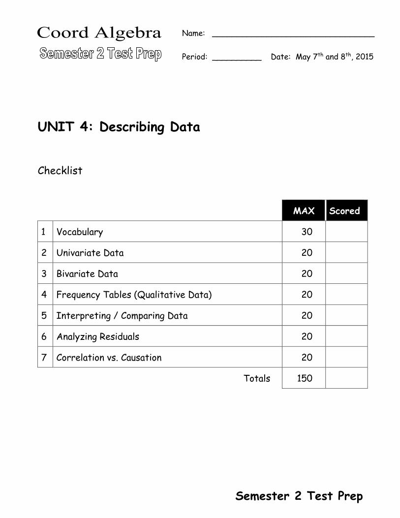
UNIT 4: Describing Data

Checklist

MAX Scored

1 Vocabulary 30

2 Univariate Data 20

3 Bivariate Data 20

4 Frequency Tables (Qualitative Data) 20

5 Interpreting / Comparing Data 20

6 Analyzing Residuals 20

7 Correlation vs. Causation 20

Totals 150

Name: _________________________________

Period: __________ Date: May 7th and 8th, 2015

Unit 4: Describing Data Name: ___________________________

2 Semester 2 Test Prep

Section 1. Vocabulary (One point each response)

Word Bank (word is used only once; not all words will be used below)

Bimodal Dot plots Minimum Range

Box-Whisker Plot Histogram Mode Residual

Census Interquartile Range Outliers Sampling

Continuous M.A.D. Q1 – 1.5 (IQR) Scatter plots

Data Maximum Q3 + 1.5 (IQR) Standard deviation

Discrete Mean Qualitative Statistical process

Distribution Median Quantitative Univariate

__________ are a collection of facts, such as numbers, words, measurements, observations or

even a description of “things”.

The _________________________ is the acts of collecting, analyzing, interpreting and

presenting data. Collecting data include the collection process (census or sampling); analyzing

data looks at data attributes, like center and spread: interpreting data include estimating or

predicting outcomes using the data attributes: and, presenting data “packages” the data into

graphs, tables, frequency distributions, etc. to help users and audiences see the results of the

statistical process.



Quantitative data fall into two broad categories. _____________ data are known as “counting

data”, where numbers are captured are whole numbers. An example is a ticket: you can only

purchase a whole ticket, not a “partial ticket”. The other broad category is _______________

data, where numbers can be captured as decimals, fractions, irrational numbers, etc. An

example is the weight of a person.

________________ data are numerical information (numbers), like height, weight, count, etc.;

________________ data are descriptive information, like color, gender, or location.

When collecting data, there are two basic classifications. A ____________ is the process of

collecting information on the whole population; ______________ is the process of collecting

information from a selected part of the population.

Analyzing data involves looking at central values and the “spread” of the data. There are three

major measures of central values: The _____________ is average value of the data set,

found by summing all the data values and dividing by the number of data points. The

___________ is the middle-most value of the data set, with 50% of the data less than this

value AND 50% of the data greater than this value. The _____________ is the number in the

data set that is part of the data the most. While the mean can be calculated directly from the

data set, the median and mode(s) are best determined by rearranging the data in order.



The “spread” of the data looks at how broad the data is scattered over the range. The

___________ (Mean Absolute Deviation) looks at the spread relative to the Mean via the

average absolute differences between the mean and each data point. A little more

sophisticated calculation of spread is the ___________________ which is based on the sum of

the residual squares.

A common way of looking at the data is to look at the quartiles. The __________ is the

difference between the ________________ (also known as Q0) and the ____________ (also

known as Q4). The _________________________ (also known as the IQR) is the middle 50%

of the data values, calculated as the difference between Q3 and Q1.

The IQR is also important for calculating ___________, which are data points that statistically

do not fit well with the data. Formulaically, the lower boundary for outliers is

______________, whereas the upper boundary for an outlier is __________________.

Another effective way to view spread is graphically. Common statistical graphing techniques

include ___________, which graph individual data points above a number line,

________________, which graph the quartile values, _____________ which group and plot

data into equal sub-groups, and _______________, which are effective when plotting bivariate

(two variable) data.



T F 1 Univariate data typically looks at one variable, while bivariate data

typically looks at two variables

2 Outliers are data that don’t fit well within the data set, and should

ALWAYS be discarded or excluded

3 Data that is skewed to the left have the “tail” on the left, whereas data

that is skewed to the right have the “tail” on the right.

4 A symmetric distribution is also known as a “normal distribution”.

5 While quartile analysis is popular, data can also be effectively stratified

into deciles or percentiles.

6. Linear or exponential regressions apply only to univariate data.

7. Frequency tables are an effective tool to analyze qualitative AND

quantitative data

8. Graphs are not necessary; they are considered “nice to have” in data

analysis.

9. Dot plots are an effective graphing tool when the data set is large or the

data is widely spread out.

10. Histograms are an effective tool to look at center and spread, and can be

used to help identify outliers.



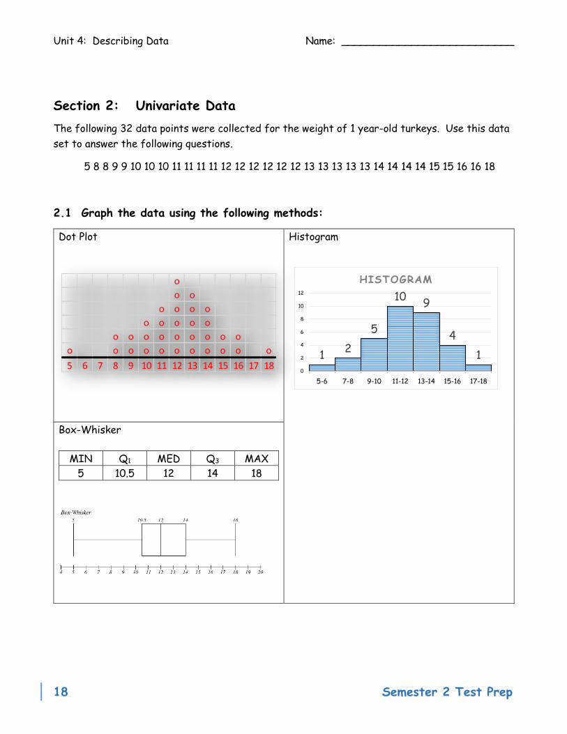
Section 2: Univariate Data

The following 32 data points were collected for the weight of 1 year-old turkeys. Use this data

set to answer the following questions.

5 8 8 9 9 10 10 10 11 11 11 11 12 12 12 12 12 12 13 13 13 13 13 14 14 14 14 15 15 16 16 18

2.1 Graph the data using the following methods:

Dot Plot Histogram

Box-Whisker

MIN Q1 MED Q3 MAX



Section 2.2: Complete the following tables of data analysis for the 32 data points:

MIN Q1 MED Q3 MAX Range IQR

Mean MAD Std.Dev Mode

Section 2.3: Determine if there are any statistical outliers using the boundary formulas.

Lower boundary:

Upper boundary:

Section 2.4: The M.A.D. (choice the right answer)

The Mean Absolute Deviation (M.A.D.) for the data set means:

a) We should be using the median as the center of measure

b) The calculation of the mean for the distribution is wrong

c) There are no outliers

d) The spread of the data is close to the mean of the distribution

Section 2.5: Describe the data set. Explain.



Section 3: Bivariate Data

The following data table provides data on ice cream sales and the high outside temperature by day.

Temp 58 62 52 60 66 74 68 80 76 74 64

Sales 215 325 185 332 406 522 412 614 544 445 408

3.1 Plot the data.

3.2 What is the best fit regression line?

3.3 What is the correlation coefficient (r)? What does it mean?

3.4 Interpret what the x-coefficient means? What does the y-intercept mean? Does

the y-intercept make sense?



Section 4: Frequency Tables

Frequency tables are a way of organizing and presenting CATEGORICAL data. A frequency

table is a table that show the total for each category or group of data. The table lists the

“frequency” or how many times the pieces of data occur.

Categorical data are data that is connected with names or labels. Gender, profession and

nationality are example of categorical data.

Joint frequencies are the body of the table; the marginal frequencies are the margins (or

totals) of the data table.

Complete the following table for 9th grader’s School Transportation Survey

Way-to-school Male Female Total

Walk 46

Car 28 45

Bus 12 27

Bike 17 69

Total 129

Answer the following questions:

a. What percentage of 9th grade girls walk to school?

b. What percentage of 9th graders are girls who walk to school?

c. What percentage of 9th grade boys bike to school?

d. What percentage of 9th graders are boys who bike to school?

e. What % of 9th graders get driven to school by a car?

f. What % is boys of the grade 9 class? Of Girls?



Section 5: Interpreting / Comparing Data

The scatter plot compares the number of bags of

popcorn sold and the number of beverage sales at a

movie theater each day for two weeks. The regression

line is estimated at B = 92.25 + 0.824 (P), where P is

bags of popcorn sold & B is beverages sold. Interpret

the following questions about the scatter plot.

1. The y-intercept represents:

A) The number of beverages sold when no popcorn is sold

B) The number of popcorn sold when no beverages are sold

C) A good estimate for the correlation coefficient

D) Nothing for this model since the value of Popcorn sales will never be zero.

2. The slope of the regression line represents:

A) The popcorn sales for a given level of beverage sales

B) The beverage sales for a given level of popcorn sales

C) The rate of increase in beverage sales for an increase in popcorn sales

D) The rate of increase in popcorn sales for an increase in beverage sales

3. What conclusion can be drawn from the scatter plot?

A) There is a negative correlation between popcorn sales and beverage sales.

B) There is a positive correlation between popcorn sales and beverage sales.

C) There is no correlation between popcorn sale and beverage sales.

D) Buying popcorn causes people to buy beverages.

4. An estimate value for the correlation coefficient would be:

A) 0.90 B) 0.50 C) -0.50 D) -0.90

5. The estimated value of beverage sales when 410 bags of popcorn are sold is:

A) 92 B) 298 C) 430 D) Cannot calculate



Section 6: Analyzing Residuals

A residual is the vertical distance between an observed data point and an estimated data

value on a line of best fit.

Residuals = actual predictedy y

A residual plot is a visual representation of the residuals.

Theory: If there is a pattern or relationship among the residuals, then there is some

functional attribute or systematic difference that has yet to be accounted for in the “best

fit” functional line. In effect, if there is a systematic difference, then the model being

used is missing something.

6.1 Identify whether or not there is a pattern.

The following residual plots have been created by charting “x” vs. the residual for the listed

linear equation. Indicate where or not you detect a pattern of systematic difference in the

graphs.

1. 2.

3. 4.

-140

-120

-100

-80

-60

-40

-20

0

20

40

0 5 10 15 20 25

Residuals



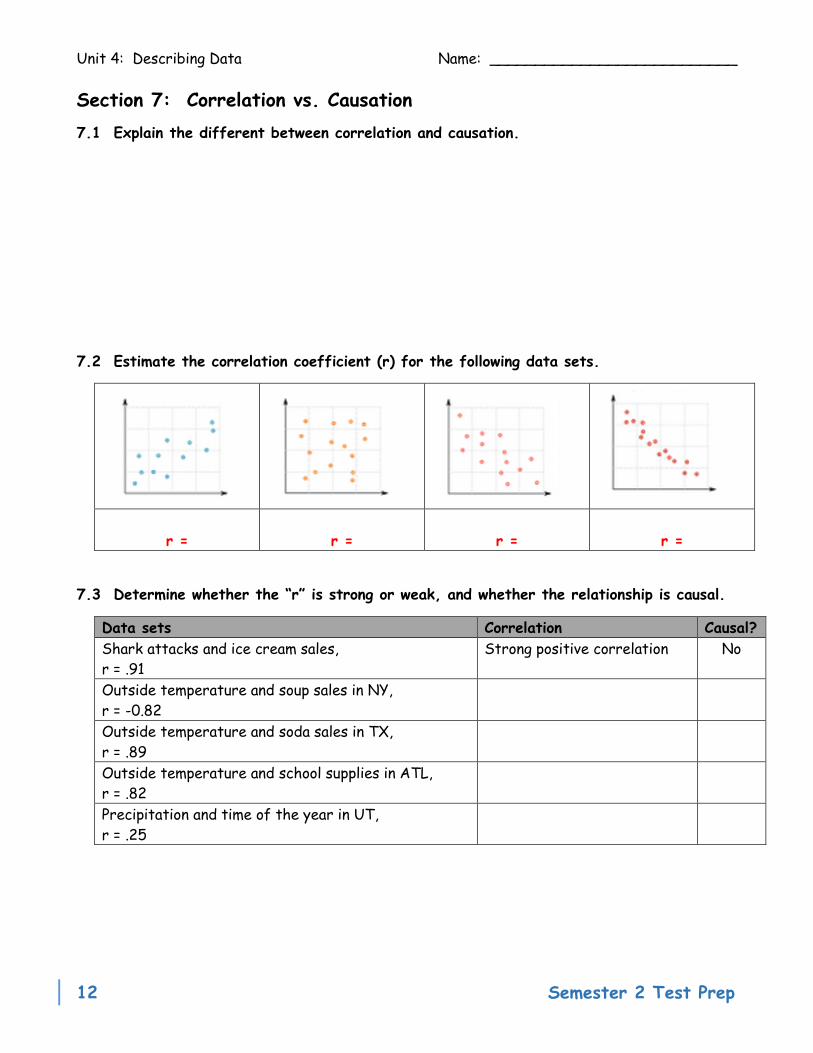
Section 7: Correlation vs. Causation

7.1 Explain the different between correlation and causation.

7.2 Estimate the correlation coefficient (r) for the following data sets.

r =

r =

r =

r =

7.3 Determine whether the “r” is strong or weak, and whether the relationship is causal.

Data sets Correlation Causal?

Shark attacks and ice cream sales,

r = .91

Strong positive correlation No

Outside temperature and soup sales in NY,

r = -0.82

Outside temperature and soda sales in TX,

r = .89

Outside temperature and school supplies in ATL,

r = .82

Precipitation and time of the year in UT,

r = .25



KEY



Section 1. Vocabulary

__________ are a collection of facts, such as numbers, words, measurements, observations or

even a description of “things”.

The __________________________ is the acts of collecting, analyzing, interpreting and

presenting data. Collecting data include the collection process (census or sampling);

analyzing data looks at data attributes, like center and spread: interpreting data include

estimating or predicting outcomes using the data attributes: and, presenting data “packages”

the data into graphs, tables, frequency distributions, etc. to help users and audiences see the

results of the statistical process.

Quantitative data fall into two broad categories. _____________ data are known as “counting

data”, where numbers are captured are whole numbers. An example is a ticket: you can only

purchase a whole ticket, not a “partial ticket”. The other broad category is _______________

data, where numbers can be captured as decimals, fractions, irrational numbers, etc. An

example is the weight of a person.

________________ data are numerical information (numbers), like height, weight, count, etc.;

________________ data are descriptive information, like color, gender, or location.

KEY

DATA

QUANTITATIVE

DISCRETE

CONTINUOUS

STATISTICAL PROCESS

QUALITATIVE



When collecting data, there are two basic classifications. A ____________ is the process of

collecting information on the whole population; ______________ is the process of collecting

information from a selected part of the population.

Analyzing data involves looking at central values and the “spread” of the data. There are three

major measures of central values: The ____________ is average value of the data set,

found by summing all the data values and dividing by the number of data points. The

___________ is the middle-most value of the data set, with 50% of the data less than this

value AND 50% of the data greater than this value. The ________ is the number in the data

set that is part of the data the most. While the mean can be calculated directly from the data

set, the median and mode(s) are best determined by rearranging the data in order.

The “spread” of the data looks at how broad the data is scattered over the range. The

___________ (Mean Absolute Deviation) looks at the spread relative to the Mean via the

average absolute differences between the mean and each data point. A little more

sophisticated calculation of spread is the ___________________ which is based on the sum of

the residual squares.

CENSUS

SAMPLING

MEAN

MEDIAN

MODE

M.A.D.

Standard Deviation



A common way of looking at the data is to look at the quartiles. The __________ is the

difference between the ________________ (also known as Q0) and the ____________ (also

known as Q4). The _________________________ (also known as the IQR) is the middle 50%

of the data values, calculated as the difference between Q3 and Q1.

The IQR is also important for calculating ___________, which are data points that statistically

do not fit well with the data. Formulaically, the lower boundary for outliers is

______________, whereas the upper boundary for an outlier is __________________.

Another effective way to view spread is graphically. Common statistical graphing techniques

include ___________, which graph individual data points above a number line,

________________, which graph the quartile values, _____________ which group and plot

data into equal sub-groups, and _______________, which are effective when plotting bivariate

(two variable) data.

RANGE

MINIMUM MAXIMUM

INTERQUARTILE RANGE

OUTLIERS

Q1-1.5 (IQR) Q3+1.5 (IQR)

Dot plots

Box-Whisker plots Histograms

Scatter Plots



T F 1 Univariate data typically looks at one variable, while bivariate data

typically looks at two variables T

2 Outliers are data that don’t fit well within the data set, and should

ALWAYS be discarded or excluded. An outlier can be discarded if

there is an error in measurement. Otherwise, it should be included

because it represents “variability” in the data set.

F

3 Data that is skewed to the left have the “tail” on the left, whereas data

that is skewed to the right have the “tail” on the right. T

4 A symmetric distribution is also known as a “normal distribution”.

T

5 While quartile analysis is popular, data can also be effectively stratified

into deciles or percentiles. T

6. Linear or exponential regressions apply only to univariate data.

Regressions apply to bivariate data. F

7. Frequency tables are an effective tool to analyze qualitative AND

quantitative data. Frequency tables apply to QUALITATIVE Data. F

8. Graphs are not necessary; they are considered “nice to have” in data

analysis. Graphs are an integral part of our analysis. F

9. Dot plots are an effective graphing tool when the data set is large or the

data is widely spread out. Dot plots are sometimes limiting when the

data sets are large and widely spread out. There are better graphs

to use (like Histograms)

F

10. Histograms are an effective tool to look at center and spread, and can be

used to help identify outliers. T



Section 2: Univariate Data

The following 32 data points were collected for the weight of 1 year-old turkeys. Use this data

set to answer the following questions.

5 8 8 9 9 10 10 10 11 11 11 11 12 12 12 12 12 12 13 13 13 13 13 14 14 14 14 15 15 16 16 18

2.1 Graph the data using the following methods:

Dot Plot Histogram

Box-Whisker

MIN Q1 MED Q3 MAX

5 10.5 12 14 18

o

o o

o o o o

o o o o o

o o o o o o o o o

o o o o o o o o o o o

5 6 7 8 9 10 11 12 13 14 15 16 17 181

2

5

109

4

10

2

4

6

8

10

12

5-6 7-8 9-10 11-12 13-14 15-16 17-18

HISTOGRAM



Section 2.2: Complete the following table of data analysis:

MIN Q1 MED Q3 MAX Range IQR

5 10.5 12 14 18 13 3.5

Mean MAD Std.Dev Mode

12.06 2.008 2.633 12

Section 2.3: Determine if there are any statistical outliers using the boundary formulas.

Lower boundary: Q1 - 1.5 (IQR) = 10.5 – 1.5(3.5) = 5.25. Thus, 5 is an outlier.

Upper boundary: Q3 + 1.5 (IQR) = 14 + 1.5(3.5) = 19.25. Thus, there are no outlier at the

top of the data set

Section 2.4: The meaning of the M.A.D.

The Mean Absolute Deviation (M.A.D.) for the data set means:

a) We should be using the median as the center of measure

b) The calculation of the mean for the distribution is wrong

c) There are no outliers

d) The spread of the data is close to the mean of the distribution

Section 2.5: Describe the data set. Explain.

The data is near-symmetric. The mean (12.06), median (12) and mode (12) indicate a strong

center value around the mean. The graphs (dot plot, histogram and box-whisker) show the data

to be almost evenly distributed around the center value. IF the outlier were excluded, the

histogram and dot plot would be tighter around the center value.



Section 3: Bivariate Data

The following data table provides data on ice cream sales and the high outside temperature by day.

Temp 58 62 52 60 66 74 68 80 76 74 64

Sales 215 325 185 332 406 522 412 614 544 445 408

3.1 Plot the data.

3.2 What is the best fit regression line?

Y (ice cream sales) = 14.864 x - 591.09.

3.3 What is the correlation coefficient (r)? What does it mean?

r = 0.967. There is a very strong positive correlation between the outside temperature and ice

cream sales.

3.4 Interpret what the x-coefficient means? What does the y-intercept mean? Does

the y-intercept make sense?

The x-coefficient means that, for every increase in temperature by one degree, ice cream sales

will increase by $14.86.

The y-intercept means at a temperature of zero degrees, there will be negative ice cream sales.

No, the intercept does not makes sense since sales cannot be negative. However, the idea that

the regression model applies to temperatures in the range of 40 and 90 degrees helps us

appreciate the model itself works as a predictive tool in the range [40,90].

y = 14.864x - 591.09

R² = 0.9353

0

100

200

300

400

500

600

700

40 50 60 70 80 90

Ice

Cre

am S

ales

Outside Temperature

Ice Cream Sales



Section 4: Frequency Tables

Frequency tables are a way of organizing and presenting CATEGORICAL data. A frequency

table is a table that show the total for each category or group of data. The table lists the

“frequency” or how many times the pieces of data occur.

Categorical data is Data that is connected with names or labels. Gender, profession and

nationality are example of categorical data.

Joint frequencies are the body of the table; the marginal frequencies are the margins (or

totals) of the data table.

Complete the following table for 9th grader’s School Transportation Survey

Way-to-school Male Female Total

Walk 34 46 80

Car 28 17 45

Bus 15 12 27

Bike 52 17 69

Total 129 92 221

Answer the following questions:

g. What percentage of 9th grade girls walk to school?

h. What percentage of 9th graders are girls who walk to school?

i. What percentage of 9th grade boys bike to school?

j. What percentage of 9th graders are boys who bike to school?

k. What % of 9th graders get driven to school by a car?

l. What % is boys of the grade 9 class? Of Girls? 41.6%

𝟒𝟔

𝟗𝟐= 𝟓𝟎%

𝟒𝟔

𝟐𝟐𝟏= 𝟐𝟎. 𝟖%

𝟓𝟐

𝟏𝟐𝟗= 𝟒𝟎. 𝟑%

𝟓𝟐

𝟐𝟐𝟏= 𝟐𝟑. 𝟓%

𝟒𝟓

𝟐𝟐𝟏= 𝟐𝟎. 𝟑%

𝟏𝟐𝟗

𝟐𝟐𝟏= 𝟓𝟖. 𝟒%



Section 5: Interpreting / Comparing Data

1. A. The y-intercept is when x = 0. In this case, Popcorn sales represent the “x” in the

graph, so the interpretation will be when P = 0.

2. C. The slope of the line is 0.824. If the sales of popcorn increase by 1 bag, then the

sale of beverages will increase on average by 0.824 units.

3. B. These is a strong positive correlation between the sale of popcorn and beverage.

Without more data and analysis, it is difficult to conclude that buying popcorn causes

people to buy beverages. Remember, the y-intercept (0, 92.25) means that when zero

bags of popcorn is sold, then 92 beverages are sold, which indicates that are other

reasons why people buy beveraes, not just popcorn.

4. A. A strong positive correlation suggests a high positive correlation coefficient. The

actual r = 0.91.

5. C. when P = 410, then B = 92.25 + 0.824 (410) = 430.



Section 6: Analyzing Residuals

6.1 Identify whether or not there is a pattern in the

The following residual plots have been created by charting “x” vs. the residual for the listed

linear equation. Indicate where or not you detect a pattern of systematic difference in the

graphs.

1. NO, there is no systematic pattern 2. YES, there is a pattern.

3. YES, there is a pattern. 4. NO, there is no systematic pattern



Section 7: Correlation vs. Causation

7.1 Explain the different between correlation and causation.

Causation is the “capacity or ability” of one variable to influence another. For example, a

first variable may:

• bring the second into existence, or

• may cause the incidence of the second variable to fluctuate.

Causation is often confused with correlation, which indicates the extent to which two

variables tend to increase or decrease in parallel. Correlation by itself does not imply causation.

There may be a third factor, for example, that is responsible for the fluctuations in both

variables. Said another way, correlation maybe a coincidence with both variables increasing or

decreasing in tandem.

7.2 Estimate the correlation coefficient (r) for the following data sets.

Modest Positive

r = 0.5

No correlation

r = 0

Modest Negative

r = -0.5

Strong negative

r = -0.9

7.3 Determine whether the “r” is strong or weak, and whether the relationship is causal.

Data sets Correlation Causal?

Shark attacks and ice cream sales,

r = .91


Outside temperature and soup sales in NY,

r = -0.82

Strong negative correlation Yes

Outside temperature and soda sales in TX,

r = .89

Strong positive correlation Yes

Outside temperature and school supplies in ATL,

r = .82


Precipitation and time of the year in UT,

r = .25

Weak positive correlation No

unit 4: describing data - wordpress.com · 5/5/2015 · unit 4: describing data name: _____ 2...

Documents