unit 5 using microsoft excel 2010 - mr. fagerlin's class...

7310-1 v1.00 © 2009 CCI Learning Solutions Inc. 251

Unit 5

Unit O

bjectives

Lesson Topic

28 Getting Started

29 Manipulating the Information

30 Working with Formulas

31 Formatting a Worksheet

32 Using Miscellaneous Tools

33 Working with Charts

34 Getting Ready to Print

This unit includes the knowledge and skills

required to analyze information in an electronic

worksheet and to format information using

functions specific to spreadsheet formatting

(as opposed to Common Elements discussed

in Unit 3). Topics include the ability to use

formulas and functions, sort data, modify the

structure of an electronic worksheet, and edit

and format data in worksheet cells. Elements

also include the ability to display information

graphically using charts, and to analyze

worksheet data as it appears in tables or graphs.

Using Microsoft Excel 2010

Un

it 5: U

sing

Micro

soft E

xce

l 20

10

L e s s o n 2 8 G e t t i n g S t a r t e d

252 7310-1 v1.00 © 2009 CCI Learning Solutions Inc.

Lesson 28 Getting Started

Objectives In this lesson, you will learn the basics of a spreadsheet program, and create some documents. On

completion, you will be able to:

understand and recognize basic terminology

create a new workbook

open a workbook

save a workbook

close a workbook

enter numeric and text information

move around in the worksheet

Skills

2-1.1.3 Navigate around open files

2-1.2.1 Create files

2-1.2.2 Open files

2-1.2.3 Switch between open documents

2-1.2.4 Save files in specified locations/formats

2-1.2.5 Close files

2-1.3.1 Insert text and numbers into a file

2-3.1.1 Identify how a table of data is organized in a spreadsheet

2-3.1.2 Identify the structure of a well-organized, useful worksheet

2-3.1.3 Insert and modify data

2-3.1.10 Identify common uses of spreadsheets (such as creating budgets, managing expense reports, or

tracking student grades) as well as elements of a well-organized, well-formatted spreadsheet

Understanding Basic Terminology 2-3.1.1 2-3.1.10

An Excel worksheet is similar to a very large sheet of paper divided into rows and columns. Rows are numbered from 1 to 1,048,576; columns are assigned letters or letter combinations from A to Z, and then AA to ZZ, then AAA to AZZ, and so on up to XFD.

Workbook A single Excel file containing one or more worksheets (Sheet1, Sheet2, Sheet3).

Worksheet A single report or tab in a workbook; each new workbook includes three worksheets.

Un

it 5: U

sing

Micro

soft E

xce

l 20

10

G e t t i n g S t a r t e d L e s s o n 2 8


Cell The intersection of a row and a column; can contain one single value (text or number), or formula.

Cell Address The column-by-row intersection designated by the column letter and the row number, such as A1 in the picture above.

Active Cell The cell currently displayed with a thick border, such as cell A1 in the picture above.

Use worksheets whenever you need a report or document that tracks numerical information. You might use Excel to create budgets, cash flow analysis reports, revenue and expense reports, financial reports, an inventory analysis, or a document tracking such data as employee vacation time or student grades.

Organize the information on the worksheet in a way that will be clear to you and anyone else who may be using or analyzing the content. Include appropriate labels and descriptions in the reports so the audience understands what they are reviewing. As there are a large number of rows and columns available, you can structure your report to show individual data blocks. For example, you may want to set up an inventory report to track stock levels that change every month, but you may also want to view a two-year period at one time. To do this, you can set up columns to show levels for each of 24 months with each row as an individual inventory item. You can also hide every month but the last six months of the previous year, or use a filter command to display information about specific inventory items.

You can use design elements to emphasize data areas such as labels, increases in sales or expenses, profit margins, highest or lowest grade, and so on. However, use discretion with design elements to ensure the report does not become difficult to read. Too much color and shading may be hard to read if it is printed on a black-and-white printer.

Working with Workbooks 2-1.2.1 2-1.2.2 2-1.2.3 2-1.2.4 2-1.2.5

When Excel starts, you are ready to begin entering data into a worksheet of a new workbook. You can also choose to open an existing workbook. A file in Excel is a workbook that, by default, contains three worksheets; this is similar to having a binder for a specific topic which then contains reports for this topic.

Creating a New Blank Workbook When you start Excel, a new workbook displays and is automatically named Book1. Each time you create a new workbook during the same session, Excel will number it sequentially as Book2, Book3, and so on. When you exit Excel and start it later, the numbering begins at 1.

To create a new blank workbook, use one of the following methods:

Click the File tab, click New, and then in the Available Templates area, click Blank workbook, and click Create; or

press + .

Exercise

1 Start Microsoft Excel and press + .

Notice that your document title bar now displays the name Book2 rather than Book1, and that there are windows for both of these workbooks when you point at Excel on the taskbar.

Un

it 5: U

sing

Micro

soft E

xce

l 20

10



Creating a New Workbook from a Template You can create a workbook using a template or pre-designed worksheet provided by Microsoft. This provides a consistent look for specific types of reports. The number of templates on your screen may vary, depending on whether an earlier version of Excel was installed previously.

To create a new workbook using a template, click the File tab, and then click New.

Exercise

1 Click the File tab and then New.

Note that a preview of any selected template displays in the right-hand pane.

2 In the Office.com Templates pane, click Inventories.

Un

it 5: U

sing

Micro

soft E

xce

l 20

10



3 Click Home contents inventory list and then click Download.

Excel now displays a blank inventory form.

You can also select from your own templates, Microsoft’s Web site, or other Web sites. To use templates from Microsoft’s Office.com site, select one of the items from the list in the Office.com Templates section of the Available Templates pane.

4 Leave the three workbooks open on the screen for the next exercise.

Opening Workbooks To work with an existing workbook, you must first open it. You can have more than one workbook open in Excel at the same time.

To open a file, use one of the following methods:

Click the File tab, then click Open. Select the file you want and click Open; or

press + ; or

click the File tab to display the most recently used files, and then click the file name to open it. You can change the number of files that display in the list using the option at the bottom of the list of files, or via Options.

You can also open a file from within the file management tool or the desktop; the operating system must recognize this file type as one that Excel can open.

Exercise

1 Click the File tab, and then click Open.

2 Navigate to where the student data files are located and select the CO2 Emission Estimates workbook.

3 Click Open.

Switching Between Workbooks When you have multiple documents open on the screen, you can switch between documents quickly and easily using one of the following methods:

On the View tab, in the Window group, click Switch Windows; or

click the button for the required document on the taskbar; or

if the Document window is in Restore Down view, the open documents may display in a cascading layout; if so, click the title bar for the appropriate document to switch to that document.

Closing Workbooks When you no longer want to work with the current workbook, save the changes and then close it to protect it from accidental changes, or to free up system resources for other files. Once closed, Excel displays other open workbooks, or a blank background screen if no other workbooks are open.

Exercise

1 On the View tab, in the Window group, click Switch Windows, then click the Book2 workbook.

2 Press + to close it.

3 On the View tab, in the Window group, click Switch Windows, then click the Home contents inventory list1 workbook.

4 Click the CO2 Emissions file on the Windows taskbar to display it.

5 Click Close Window to close this file.

Un

it 5: U

sing

Micro

soft E

xce

l 20

10



Saving Workbooks To use a file again, you must save the workbook. It is a good practice to save work frequently during a session, especially if the workbook is large, or if you are using a process you have not tried before.

There are two types of save commands:

Use Save As to save a new or existing file with a new name, location, or file format.

Use Save to save changes in the active file, thereby replacing the contents of the existing file in this location.

To save the changes made to an existing file, use one of the following methods:

Click the File tab and then Save; or

on the Quick Access toolbar, click (Save); or

press + .

The first time you save a file, you will always see the Save As dialog box so that you can give the new workbook a distinct name and select the location where it will be stored, such as the hard drive, network drive, or portable media drive. By default, Excel navigates to the Documents folder as the location to save the file. You can choose this location or navigate to another location using the Save in field. You can also create new folders within Excel during the save process.

To save the changes made to an existing file and save it with a new name or in a different file format, click the File tab and then click Save As.

To save the file in another file format, click the arrow for the Save as type field to select the appropriate file type.

One example of a file format you may need to use is .xltx (Excel Template), which will save the file as a template. A template is a combination of pre-designed formats and styles that you customize for a specific type of report and save for future use. Another example of a file type you may need is the .csv (Comma Delimited), which makes it possible for the file to be exported into another program, such as Access. Or you may simply need to save a file to be compatible with an earlier version of Excel, such as Excel 2003.

Exercise

1 If necessary, select the Home contents inventory list1 workbook.

2 Click the File tab and then Save.

Excel presented the Save As dialog box as this is the first time you are saving this workbook. Notice also that the file name highlights in the File name field; whenever a file name is highlighted as seen here, you can type a new name to replace the existing text. You do not have to click the mouse anywhere in the file name area.

3 In the File name field, type: Home Inventory ‐ Student.

4 Click Save.

The title bar now displays the name Home Inventory - Student.

To save the file in a new location other than the default, which is generally \Documents, you can move to a different location or create a new folder. In this exercise, you will create a new folder in the same location as your student data files and save the file with the same name.

5 Click the File tab and then Save As.

Un

it 5: U

sing

Micro

soft E

xce

l 20

10



6 Click New folder in the Command Bar.

7 Type: Forms as the name of the new folder and click Open.

8 Leave the file name as is and click the Save button.

You now have a copy of the same file in the default folder as well as the new folder just created.

9 Press + to close this file.

Entering Data in the Worksheet 2-1.1.3 2-1.3.1 2-3.1.1 2-3.1.2 2-3.1.3

You can insert three types of data into worksheet cells:

Labels Text entries appear in the cells exactly as you enter them; default as left aligned.

Values Numeric values; default to right aligned.

Formulas Composed of cell references, arithmetic operators, and functions that operate on data.

Entering these types of data into a single workbook with multiple worksheets allows you to organize the data into a three dimensional structure. For example, when you open a file the main worksheet may summarize company expenses from all departments for one year, but each individual entry may be a total of values from subsequent sheets for each department. Excel provides the flexibility to enter data into different worksheets that link to other worksheets in the same or other workbooks.

Entering Text or Labels To enter information, click on the cell to select it and then type the entry. Use the key or key to correct any input errors. When you finish typing, press to move to the next cell below. You can also click another cell or press any arrow key to accept the input in the current cell.

The best way to begin any worksheet is to enter labels that identify the values, or an outline of the relationships you will later represent mathematically. For example, the report shown here has a label indicating one of four quarterly intervals. Each row beneath the column labels shows the results for that quarter in the noted region. You can then see how the revenue figures increase or decrease for Region 1 as you follow from Q1 to the Total column.

When entering information, consider the following:

You can enter or edit data directly in the active cell, or use the Formula bar for long data entries.

Labels can be up to 32,767 characters long.

If a label is longer than the width of the cell, it will display past the column border as long as the adjoining cells are empty. Entries in adjoining cells cut off the display at the column border. The long text label may not be visible, but it is still in the cell where it was entered.

You can easily change the appearance and alignment of any label in any cell.

The maximum length of formula contents is 8,192 characters.

Un

it 5: U

sing

Micro

soft E

xce

l 20

10



Entering Numbers or Dates Numbers are constant values such as dollars and percentages; by default, they align to the right side of a cell. If you enter characters other than numbers, Excel treats the entry as a label. Excel displays values with no formatting, allowing you to format them yourself.

When entering dates, you can enter them in a numeric form (i.e., 2-26-05) or as text (i.e., Month day, year). When entering dates, note the following:

The default format of the date value is m-d-yy, although you can change this using the Region and Language in the Control Panel.

The date value does not have to be the full day, month, and year. It can be just the day and month (formatted mmm-dd), or the month and year (formatted mmm-yyyy).

When entering a date, Excel does its best to interpret what you enter, as with these acceptable date values:

September 13, 2002 (include the comma and one space)

Sep 13, 02

13-Sep-02

09/13/02 (month, day, year sequence)

9-13-02

Sep 2002

Sep 13

If Excel cannot interpret the date value, it will appear as a text label and potentially cause problems in the worksheet if this date value is to be included in any formulas.

Moving Around the Worksheet You can move around the cells of a worksheet using one of the following methods:

Scroll Bars Click the arrow buttons at either end to move one row or column at a time. Click and drag the scroll box to display another location in the worksheet.

, , , Press one of the direction keys to move one cell at a time.

Move to column A in the current row.

+ Move to cell A1.

+ Move to the last cell in your data.

+

Display the Go To dialog box to move quickly to a cell reference, range name, orbookmark, or use the Special button to find specific types of information.

Exercise

1 Click the File tab and then Open.

Notice how Excel displays the last location you used to save or open a file.

2 Navigate to the level for your student data files and then open Home Inventory - Student.

3 Click the File tab and then Save As.

4 Type: Home Inventory JM ‐ Student as the new name for this workbook, and then click Save.

5 With the cursor in cell C3, type: Jane Martinez as the name of the owner.

6 Click cell B14 and type: Family Room for the Room/area.

7 Click cell C14 and type: Big screen TV for the Item description. Press three times to move to the Date purchased column and type: March 23, 2010. Press once more.

Notice how Excel has changed the date to the format this form uses for dates. At this point, you would continue to enter the information you know or have for this particular inventory item. For the purpose of this exercise, you will enter some basic information.

8 Enter the remaining values as shown in the following:

Un

it 5: U

sing

Micro

soft E

xce

l 20

10



Room/area Item/description Make/model Date purchased Family Room Big screen TV 3/23/10

Family Room Gaming system 4/7/10

Family Room Gaming system 2/22/09

Family Room Blu‐ray player 3/23/10

Kitchen TV/DVD Combo 7/23/09

Kitchen Food processor Kitchen Aid

Kitchen Coffee maker Mr. Coffee

Notice how as you enter the similar values, Excel automatically displays the item so you can press or to accept this value. This is known as the AutoComplete feature where Excel will try to

help you with data entry if it detects the entry shares characters in another cell.

9 Save and close the workbook.

Summary In this lesson, you learned the basics of a spreadsheet program, and created some new documents. You

should now be able to:

understand and recognize basic terminology

how to create a new workbook

open a workbook

save a workbook

close a workbook

enter numeric and text information

move around in the worksheet

Review Questions 1. There is no difference between a workbook and a worksheet.

a. True b. False

2. A cell is: a. Any box in the worksheet b. The grey boxes at the top or left of the worksheet identifying the columns or rows c. The intersection of a column and a row d. All of the above e. a or c

3. Which command would activate the Template dialog box to create a new workbook? a. On the Quick Access toolbar, click New. b. Click the File tab, click New. c. Press + . d. Click the Blank Workbook link on the Getting Started task pane

4. Use the Save command when you want to save changes made to an existing document, and the Save As command when you want the file to have a different file name. a. True b. False

5. It is important to identify the data in the worksheet by using labels to describe what the values represent, such as monthly values, department expenses, and so on. a. True b. False

Un

it 5: U

sing

Micro

soft E

xce

l 20

10

L e s s o n 2 9 M a n i p u l a t i n g t h e I n f o r m a t i o n


Lesson 29 Manipulating the Information

Objectives In this lesson, you will learn to select items in a worksheet for the purpose of making changes or manipulating

the data. On completion, you will be able to:

select cells or ranges of cells

make changes to the cell contents

use Undo and Redo

copy and move data

change column widths and row heights

insert and delete rows and columns

fill cells with contents automatically

manage worksheets

Skills

2-1.3.2 Perform simple editing

2-1.3.3 Use the Undo, Redo and Repeat commands

2-3.1.3 Insert and modify data

2-3.1.4 Modify table structure

Selecting Cells 2-1.3.2

Prior to performing an action, you must indicate what range or part of the spreadsheet to affect with that action. A range can be a single cell, several cells, or the entire spreadsheet. These cells remain selected or highlighted until you click a cell or press an arrow key. The selected range appears in reverse color to the cells. The active cell in the selected range appears in normal color. You can highlight individual cells or any range of cells as follows:

A single cell Click the cell.

Extend the selection Click the first cell and drag to the end of the required range; or click the first cell,hold the key, and click the end cell in the range.

An entire row Click the row header when you see the (row heading symbol).

An entire column Click the column header when you see the (column heading symbol).

The entire worksheet Click the Select All button.

Non-adjacent columns, rows, or cells

Click the cell, column, or row, hold the key, then click to select the next cell, column, or row; you can also drag to select multiple cells.

Multiple rows Click the first row number and drag for the number of rows you want to select.

Multiple columns Click the first column letter and drag for the number of columns you want to select.

Un

it 5: U

sing

Micro

soft E

xce

l 20

10

M a n i p u l a t i n g t h e I n f o r m a t i o n L e s s o n 2 9


Making Changes to the Contents 2-1.3.2 2-1.3.3 2-3.1.3 2-3.1.4

The easiest way to change cell contents is to enter the entire new content, press and have Excel replace the old information with the new entry. To correct errors as you type, press or prior to pressing or moving to another cell.

If you want to add, delete, or change less than the entire contents of the cell, you can activate Excel’s Edit mode by pressing or double-clicking on the cell; Excel will display the insertion point and you can proceed in one of the following ways:

Select the text in the cell, type in the replacement text, and press to exit the Edit mode; or

press the key to turn on Overtype mode, and replace existing text with whatever you type; or

use the key to remove any unwanted characters from the cell contents.

Using Undo, Redo, or Repeat Excel has an Undo function that enables you to undo commands executed in the worksheet.

Excel can undo up to a maximum of 100 commands recently used. This “undo history” displays when you click the down arrow beside the Undo button. The Undo command can only be performed in the reverse sequence of the changes done to the worksheet; you cannot reverse the changes in a sequence of your choosing. Undo does not work for some commands such as saving the file.

If you need to reverse an undo, you can redo (“un-undo”) it. The Redo function is only available if one or more commands were undone.

Excel keeps a history of the last 100 actions that were undone for the Redo feature. To display the redo history, click the down arrow beside the Redo button. Like the Undo command, the Redo commands must be performed in the reverse sequence of the actions that were undone.

You can also repeat the most recent action by using the key.

Copying and Moving Data Excel enables you to copy or move cell contents from a different part of the same worksheet, another worksheet in the same workbook, or a worksheet in a different workbook.

Cut Removes the contents of a cell or a range to the Office Clipboard.

Copy Copies the contents of a cell or a range of cells to the Office Clipboard.

Paste Pastes any or all contents from the Office Clipboard in one or more cell locations.

Paste Special Modifies the effects of the paste option, such as by pasting the contents or format only.

Before you can activate the copy or cut command, you need to select a range; when you do, a marquee (moving dotted rectangle) will appear around the selection, identifying what you want to cut or copy. To remove the marquee, use one of the following methods:

Press ; or

type the first letter, number, or symbol on a new entry; or

press to paste the cut or copied item into this location only.

Note that when you press or use the Cut command, the information is removed, but any formatting applied to that data will still exist in that location. You must use the Clear command for more choices regarding deletion. The command is on the Home tab, in the Editing group.

Un

it 5: U

sing

Micro

soft E

xce

l 20

10



Using the Office Clipboard You can cut or copy more than one cell range, and keep up to 24 cell ranges in the Office Clipboard at one time. You can then paste any or all these items in any sequence.

Activate the commands for cut, copy, and paste using the Home tab, in the Clipboard group, or with the keyboard shortcuts. Display the Office Clipboard at any time by clicking the Dialog box launcher in the Clipboard group of the Home tab.

Exercise

1 Press + to create a new blank workbook and save this as TEC Executive Team ‐ Student.

2 Open the TEC Employee List workbook and then select cells A1 to C1.

3 On the Home tab, in the Clipboard group, click .

4 Switch to the new workbook and then in cell A1, on the Home tab, in the Clipboard group, click Paste.

5 Switch to the TEC Employee List workbook.

The headings for the first three columns in the report should no longer appear.

6 As you did not want to move the headings from this report, on the Quick Access toolbar, click (Undo).

Notice how Excel automatically removes the headings from the blank report and keeps this displayed.

7 Switch to the TEC Employee List.

The headings appear again in this report and the marquee appears around the selected cells.



10 Switch to the TEC Employee List to see if the headings still appear here as well.

Using the Copy command keeps the original information intact whereas the Cut command physically removes the information from the location and places it in the new location.

11 Click cell A2 and drag to select from here to cell C4.



14 Switch to TEC Employee List, and select cells A20 to C20. Press and then select cells A24 to C24.

15 Press + to copy these cells and then switch to the new workbook.

16 In cell A5, press + to paste the cells in this location.

17 Switch to the TEC Employee List and close this workbook without saving.

18 Save the TEC Executive Team - Student workbook again.

Un

it 5: U

sing

Micro

soft E

xce

l 20

10



Using Fill Use the Fill feature to automatically fill in data based on the original contents; this could be data in a single cell, or a range of cells where a specific pattern or trend exists in that range.

To use the Fill option, use one of the following methods:

On the Home tab, in the Editing group, click the button; or

select the cell range with the data to fill, position the mouse pointer at the lower right corner of the range, and when you see the thick crosshair, drag to the required number of cells.

Exercise

1 Open the TEC Project Consultants Report and save as TEC Project Consultants Report ‐ Student.

2 In cell D2, type: Number of Projects.

3 In cell D3, type: Apr and press .

4 Click cell D3 to select it and then point the cursor at the lower right corner, where the small black box appears.

5 With the small crosshair symbol active, click and drag to the right to cell H3.

The headings should then appear similar to the following:

6 Click the Auto Fill Options button to view the options.

Un

it 5: U

sing

Micro

soft E

xce

l 20

10



Excel recognizes that you used the Fill command to quickly insert the data for these cells. You could choose any of the options here to change the information as required.

7 Click anywhere away from the button to close this option.

8 Save the workbook.

Now try using the Auto Fill option in different ways.

9 Click the Estimates tab to go to this worksheet.

10 Select cell C1, then position the cursor at the lower right corner of cell C1 and drag to G1.

Notice how this time the years did not change for you. This is because Excel did not recognize a pattern or a known trend in the original cell. As a result, Excel only copied the contents from cell C1 through to cell G1.

11 On the Quick Access toolbar click (Undo).

12 Click cell D1 and type: 2013.

13 Select cells C1 to D1 and then with the cursor on the Auto Fill symbol at the lower right corner of cell D1, drag to cell G1.

The years should now be correct.

Now try setting up a series where each location is estimated to grow the number of projects by seven each year. This is a rough estimate based on potential market trends; we want to determine where we may need to increase staff should the number of projects exceed what we can currently manage.

14 Select cells B2 to G7. Then on the Home tab, in the Editing group, click Fill and then Series.

15 Select the following options:

16 Click OK.

Excel has now entered in the values based on the series you used to determine a linear growth. Notice also how the Shibuya-ku location does not have a value for the 2014 year, which is a clear indicator we need to ensure we hire more staff for that location by 2012.


Changing the Column Widths You can adjust column widths to display more characters. When an entry in a cell is longer than the standard column width, Excel displays the label by overflowing the entry into the next cells if they are empty. However, if there are entries in the adjoining cells, the entry is truncated at the column boundary, as seen in the following:

Un

it 5: U

sing

Micro

soft E

xce

l 20

10



Column widths can be set between zero and 255 characters. When you change a column width, the stored contents of the cells do not change, only the number of the characters displayed.

If you enter values that exceed the column width, Excel stores the data but displays the number in scientific format. If the data is a text or date value, it appears with # symbols. Once you change the width of the cell sufficiently, Excel shows the full value properly using the assigned cell formatting.

To change the width of a column, use one of the following methods:

On the Home tab, in the Cells group, click Format, and then Column Width; or

position the mouse pointer on the line at the right edge of the column header to be adjusted; when you see (thick horizontal double-headed crosshair), click and drag to the required width for the column.

To check the width of a column, click the right edge of the column header. The width will be displayed in a screen tip above the mouse pointer.

Adjusting the Row Height When you need to adjust the row height so the row is smaller or larger than others in the worksheet, use one of the following methods:

On the Home tab, in the Cells group, click Format, and then Row Height; or

Place the mouse pointer at the bottom edge of the row header to be adjusted. When it changes to (thick vertical double-headed crosshair), click and drag to the height required.

Using AutoFit The AutoFit feature automatically adjusts the width of a column or the height of a row so that it will accommodate the longest value in the column or the text height or number of lines of text, in the row.

To adjust the width of a column using AutoFit, use one of the following methods:

On the Home tab, in the Cells group, click Format, and then AutoFit Column Width.

Double-click the line at the right edge of the column header to adjust.

To adjust the height of a row using AutoFit, use one of the following methods:

On the Home tab, in the Cells group, click Format, and then AutoFit Row Height.

Double-click the line at the bottom edge of the row header to adjust.

Exercise

1 Ensure the TEC Executive Team - Student workbook is active.

2 Click the column heading for column A and drag across to include column B.

3 Place the cursor on the vertical line between columns A and B.

4 Click and drag until the width in the ScreenTip shows as 11.00.

Un

it 5: U

sing

Micro

soft E

xce

l 20

10



Note: If you select the entire row using the row heading or the entire column using its column heading, you can just click Insert on its own. Excel automatically recognizes what to insert based on the selection of the entire row or column.

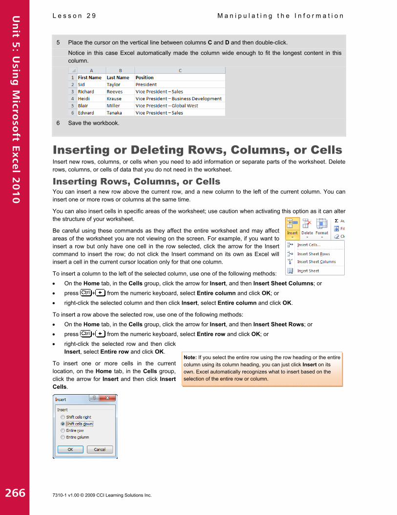
5 Place the cursor on the vertical line between columns C and D and then double-click.

Notice in this case Excel automatically made the column wide enough to fit the longest content in this column.


Inserting or Deleting Rows, Columns, or Cells Insert new rows, columns, or cells when you need to add information or separate parts of the worksheet. Delete rows, columns, or cells of data that you do not need in the worksheet.

Inserting Rows, Columns, or Cells You can insert a new row above the current row, and a new column to the left of the current column. You can insert one or more rows or columns at the same time.

You can also insert cells in specific areas of the worksheet; use caution when activating this option as it can alter the structure of your worksheet.

Be careful using these commands as they affect the entire worksheet and may affect areas of the worksheet you are not viewing on the screen. For example, if you want to insert a row but only have one cell in the row selected, click the arrow for the Insert command to insert the row; do not click the Insert command on its own as Excel will insert a cell in the current cursor location only for that one column.

To insert a column to the left of the selected column, use one of the following methods:

On the Home tab, in the Cells group, click the arrow for Insert, and then Insert Sheet Columns; or

press + from the numeric keyboard, select Entire column and click OK; or

right-click the selected column and then click Insert, select Entire column and click OK.

To insert a row above the selected row, use one of the following methods:

On the Home tab, in the Cells group, click the arrow for Insert, and then Insert Sheet Rows; or

press + from the numeric keyboard, select Entire row and click OK; or

right-click the selected row and then click Insert, select Entire row and click OK.

To insert one or more cells in the current location, on the Home tab, in the Cells group, click the arrow for Insert and then click Insert Cells.

Un

it 5: U

sing

Micro

soft E

xce

l 20

10



Deleting Rows, Columns, or Cells You can delete one or several rows or columns, or shift cells over in place of deleted cells. Deleting the contents of a cell only affects the contents, not the structure of the worksheet as it would if you were to delete the cell.

Be careful when deleting entire rows or columns to ensure you do not accidentally delete valuable data not currently displayed on the screen.

To delete the selected column, use one of the following methods:

On the Home tab, in the Cells group, click the arrow for Delete, and then Delete Sheet Columns; or

press + from the numeric keyboard, select Entire column and click OK; or

right-click the selected column and then click Delete, select Entire column and click OK.

To delete the selected row, use one of the following methods:

On the Home tab, in the Cells group, click the arrow for Delete, and then Delete Sheet Rows; or

press + from the numeric keyboard, select Entire row and click OK; or

right-click the selected row and then click Delete, select Entire row and click OK.

To delete one or more cells in the current location, on the Home tab, in the Cells group, click the arrow for Delete, and then click Delete Cells.

Exercise


2 Click cell A1. On the Home tab, in the Cells group, click the arrow for Insert and then click Insert Sheet Rows.

3 Press to repeat the process of inserting a new blank row in this location.

4 In cell A1, type: Tolano Executive Team Members and press .

The blank row between the title and the data provides more space between the two sets of data. However, the spacing is too much. You can change this by adjusting the height of this row.

5 Position the cursor on the bottom of the row 2 heading.

6 Click and drag upwards until you see 6.00 in the ScreenTip.

Suppose you decide you no longer need this blank row.

Note: If you select the entire row using the row heading or the entire column using its column heading, you can just click Delete on its own. Excel automatically recognizes what to delete based on the selection of the entire row or column.

Un

it 5: U

sing

Micro

soft E

xce

l 20

10



7 With the cursor still in row 2, on the Home tab, in the Cells group, click the arrow for Delete and then click Delete Sheet Rows.

8 Save the worksheet.

Managing Worksheets 2-3.1.4

A workbook is a collection of worksheets. While each worksheet can be treated as an independent spreadsheet, information on the worksheets is typically inter-related.

Worksheets can be renamed, added, deleted, copied, and moved within a workbook. Use the tab scrolling buttons to display more worksheet tabs as required.

Naming Worksheets Sheet1, Sheet2, Sheet3, and so on help to identify different sheets as you create them, but do not describe their contents, which can make it difficult for you to find what you want. Renaming tabs with more descriptive names makes navigation easier. Worksheet tabs can be up to 31 characters long.

To rename a worksheet tab, use one of the following methods:

On the Home tab, in the Cells group, click Format, and then Rename Sheet; or

double-click the sheet tab and then type the new name.

Inserting or Deleting Worksheets Excel automatically includes three worksheets with a new workbook, but you can add more. To insert a new worksheet, use one of the following methods:

On the Home tab, in the Cells group, click Insert, and then Insert Sheet; or

in the sheet tabs area, click (Insert Worksheet) to automatically add a worksheet at the end of current worksheet tabs; or

press + ; or

right-click the tab where you want to place the new sheet, click Insert, Worksheet, and then click OK.

Use the tab scrolling buttons to display more worksheet tabs, or adjust the length of the horizontal scroll bar.

Deleting worksheets that you no longer need can help keep your workbook easy to use, but consider saving the workbook before deleting a worksheet in case you need to revert to the previous version of the file. Note that the Undo command does not work for a deleted worksheet. Also, check every worksheet for any errors in case there were formulas that affect the values in the rest of the worksheets.

To delete a worksheet, select the sheet and then use one of the following methods:

On the Home tab, in the Cells group, click the down arrow for Delete, and then Delete Sheet; or

right-click the sheet tab and click Delete.

4

2 1

1

2

First

Next

3

4

Previous

Last

3

Un

it 5: U

sing

Micro

soft E

xce

l 20

10



Exercise


2 Double-click the Sheet1 tab, type: Executives and press .

3 Double-click the Sheet2 tab, type: Managers and press .

4 Double-click the Sheet3 tab, type: Project Consultants and press .

5 Click (Insert Worksheet).

6 Double-click the Sheet4 tab, type: Staff and press .

This report will contain the names only of the Executive Team and Managers. You need to delete the last two worksheets.

7 Right-click the Staff tab and then click Delete.

8 Right-click the Project Consultants tab and then click Delete.


Summary In this lesson, you learned to select items in a worksheet for the purpose of making changes or manipulating

the data. You should now be able to:

select cells or ranges of cells

make changes to the cell contents

use Undo and Redo

copy and move data

change column widths and row heights

insert and delete rows and columns

fill cells with contents automatically

manage worksheets

Review Questions 1. When you activate the Cut or Copy command, a marquee appears around the selected cell(s). How can you

remove the marquee? a. Press . b. Press . c. Continue entering data in new areas. d. Any of the above e. a or c

2. The Fill feature reviews the contents or patterns in selected cells and then fills adjacent cells with corresponding data, based on the trend or type of data in the selected cells. a. True b. False

3. How can you adjust the width of a column? a. On the Home tab, in the Cells group, click Format, click Column Width. b. On the Home tab, in the Cells group, click Format, click AutoFit Column Width. c. Click and drag the line at the right of the column heading. d. Any of the above e. a or c

4. When you insert a new row, where does it go? a. Above the current row b. Below the current row

5. You cannot change the names of each of the sheets. a. True b. False

Un

it 5: U

sing

Micro

soft E

xce

l 20

10

L e s s o n 3 0 W o r k i n g w i t h F o r m u l a s


Lesson 30 Working with Formulas

Objectives In this lesson you will learn to work with formulas, including creating simple formulas and using some of the

built-in functions. On completion, you will be able to:

identify formulas

structure formulas

use some common built-in functions

understand what absolute and relative formulas are

use formulas correctly

Skills

2-3.2.3 Demonstrate an understanding of absolute vs. relative cell addresses

2-3.2.4 Insert arithmetic formulas into worksheet cells

2-3.2.5 Demonstrate how to use common worksheet functions

2-3.2.6 Use AutoSum

2-3.2.7 Insert and modify formulas and functions

2-3.2.8 Identify common errors people make when using formulas and functions

Creating Simple Formulas 2-3.2.3 2-3.2.4 2-3.2.5 2-3.2.6 2-3.2.7

A formula is a calculation using numbers (or other data) in a cell or from other cells, such as:

automatically calculating sums horizontally and vertically

performing “what-if” analyses by performing a calculation based on one or more changed input value, such as estimated profit for a business during the next year

using one or more Excel functions to perform tedious or complex calculations, such as monthly mortgage payments.

Formulas can be linked from one worksheet to another, so that when you change values or amounts in the active worksheet, dependent cells in the other worksheet will be automatically updated. You can use a single cell as the reference point, or you can create complex formulas with many cell references as well as built-in functions.

To begin a formula in any cell, you must type an equal sign (=). You can enter a cell address into a formula either by typing it directly into the cell, or by pointing to the cells to be included. The cell will then display the result of the formula; the formula itself will be displayed in the Formula bar.

Some formulas are long with many calculations. If you need to change a formula, you can use the key to change the formula in the cell, instead of entering the entire formula from scratch.

Cells containing formulas can be copied to other cells. If these formulas contain cell references, Excel will automatically adjust the cell references for you to speed up the construction of data tables.

Excel calculates formulas in “natural order”: exponents first, then multiplication and division, and then addition and subtraction. This order can be altered by inserting parentheses around portions of the formula; Excel will calculate the portions in parentheses before calculating the other items in the formula.

Un

it 5: U

sing

Micro

soft E

xce

l 20

10

W o r k i n g w i t h F o r m u l a s L e s s o n 3 0


The following shows the symbols used in Excel to represent standard mathematical operators:

* Multiplication + Addition

/ Division - Subtraction

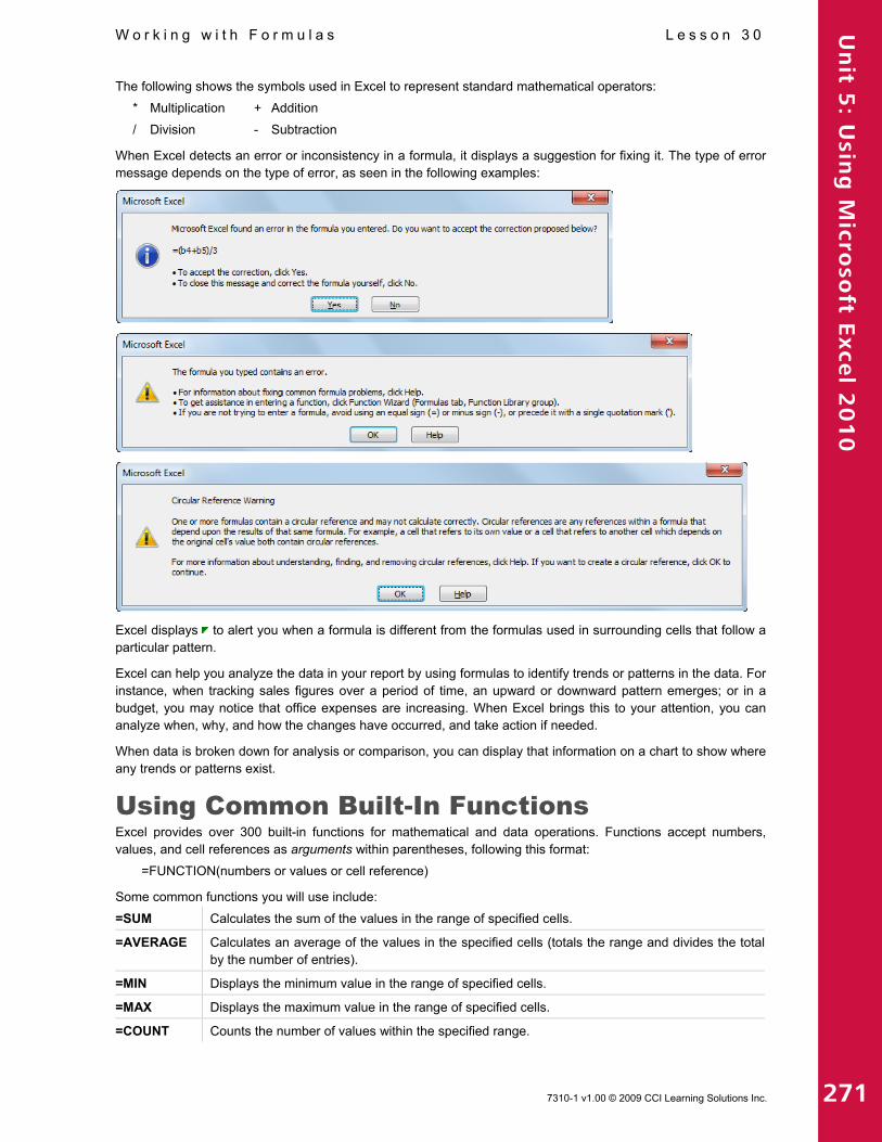
When Excel detects an error or inconsistency in a formula, it displays a suggestion for fixing it. The type of error message depends on the type of error, as seen in the following examples:

Excel displays to alert you when a formula is different from the formulas used in surrounding cells that follow a particular pattern.

Excel can help you analyze the data in your report by using formulas to identify trends or patterns in the data. For instance, when tracking sales figures over a period of time, an upward or downward pattern emerges; or in a budget, you may notice that office expenses are increasing. When Excel brings this to your attention, you can analyze when, why, and how the changes have occurred, and take action if needed.

When data is broken down for analysis or comparison, you can display that information on a chart to show where any trends or patterns exist.

Using Common Built-In Functions Excel provides over 300 built-in functions for mathematical and data operations. Functions accept numbers, values, and cell references as arguments within parentheses, following this format:

=FUNCTION(numbers or values or cell reference)

Some common functions you will use include:

=SUM Calculates the sum of the values in the range of specified cells.

=AVERAGE Calculates an average of the values in the specified cells (totals the range and divides the totalby the number of entries).

=MIN Displays the minimum value in the range of specified cells.

=MAX Displays the maximum value in the range of specified cells.

=COUNT Counts the number of values within the specified range.

Un

it 5: U

sing

Micro

soft E

xce

l 20

10



Cell ranges in a function should be set up as follows:

<first cell address>:<last cell address>

Examples:

A10:B15, C5:C25

You can specify the range by typing the cell reference directly or by using the “point-to” method, where you use the mouse to click and drag to select the cell range. The latter method allows you to visually identify the cell range, which reduces the chance that you will enter incorrect cell references.

When calculating totals, you can use on the Home tab in the Editing group. Excel then selects the range of cells immediately above or to the left of the current cell.

Be sure to verify that you have selected the correct cell range for the function. If there is even one blank cell between cells, the range may not include all cells.

Use the arrow next to the tool to display other common built-in functions, or use More Functions to choose a different function.

Exercise

1 Open the North America GHG Report workbook and save as North America GHG Report ‐ Student.

2 In cell D5, type: =c5‐b5 and press .

Excel now calculates the value and displays it in the cell. As you entered the cell addresses, Excel also highlighted these cells in different colors as a visual indicator to which cells are used or referenced in the formula.

3 Click cell D5 and view the contents in the Formula bar.

Remember that Excel always displays the results of the formula in the cell of the worksheet although the contents of the cell contain the actual formula, as shown in the Formula bar. Notice also how the cell addresses are not case sensitive.

Try setting a formula using the point and click method instead of typing the formula in directly.

4 In cell D6, type: = to begin the formula and then click cell C6.

Un

it 5: U

sing

Micro

soft E

xce

l 20

10



5 Type: ‐ (dash to indicate the subtraction operator) and then click cell B6. Press .

The result now appears in cell D6.

The two preceding formulas were examples of simple formulas you can create. They are considered simple as they are relatively small and only involve the use of arithmetic operators with no functions. Now try using some built-in functions to calculate a larger set of cells.

6 In cell B12, on the Home tab, in the Editing group, click .

Notice how Excel displays a marquee to indicate which cells will be included in the formula, as well as displays the formula. Whenever multiple cells are used in a formula, they display a colon between the first cell in the range and the last cell in the range.

7 Press to accept the formula.

You can also use the point and click method, if preferred, with built-in functions.

8 In cell C12, type: =sum( to begin the formula. Be sure to include the open bracket to tell Excel you will now be indicating the cell range.

9 Starting at cell C5, click and drag to cell C11.

Notice Excel provides a very similar display as if you used the Sum function as in step 6.

10 Press to accept the formula.

The formula should have had a closing bracket “)” at the end. When you pressed the key, Excel knew it was needed and added it for you. You should try to enter all closing brackets manually to ensure that Excel does not add them in the wrong places for you.

11 In cell E5, type: =(c5‐b5)/b5 and press .

Un

it 5: U

sing

Micro

soft E

xce

l 20

10



The formula you are now calculating is the percentage change from 1990 to 2006, or =(2006-1990)/1990.


Now try creating the formulas for another worksheet so you can eventually create a new worksheet that shows a summary of the changes for North America from 1990 to 2006.

13 Click the US tab.

14 In cell B10, on the Home tab, in the Editing group, click .

Notice how the sum formula includes the year cell in the range—you do not want this option.

15 Starting with cell B3, click and drag to select to cell B9.

16 Press when the formula shows as =SUM(B3:B9).

While there are other years in the US report, we only want to compare 1990 and 2006 figures as those are the only years available in the Canada worksheet.

17 In cell F10, type: =sum(f3:f9) and press .

18 On the navigation bar across the bottom of the workbook, click (Insert Worksheet).

19 Double-click the Sheet1 tab, type: Summary and press .

20 Type the following information:

21 In cell B3, type: = to begin the formula.

22 Click the Canada sheet tab, then click in cell C12 and then press .

23 Click cell B3 again to view the contents in the Formula bar.

This is an example of how you can set up 3D worksheets by using cell addresses in other worksheets of the same report. You can also use cell addresses from another workbook, as required, but the workbook needs to be open and active on the screen to accomplish this. Excel will include the name of the worksheet and the workbook in the formula as a guide for you to see where the original data exists.

24 In cell B4, type: = to begin the formula. Click the US tab, click in cell F10, and then press .

25 Complete the other two formulas for the 1990 year.

Now try using some other common built-in functions with the Canadian and US statistics for 2006.

Un

it 5: U

sing

Micro

soft E

xce

l 20

10



26 In cell C3, type: =av to begin the Average function.

Excel provides a hint for you as you type the first few characters of the formula, as well as displays a brief explanation of how each function works.

27 Double-click the AVERAGE option and then click the Canada tab.

28 Select cells C5 to C11 and then press .

29 Click cell C3 and review the formula in the Formula bar.

Notice how Excel references the worksheet with this formula as it did with the simple formula in cell B3.

30 Use the same cell range for the next two formulas using the =MIN and =MAX functions.

31 Repeat steps 26 to 30 using the US worksheet and cells F3 to F9.

32 Save the workbook again.

Using Absolute and Relative Addresses Most formulas entered into an Excel worksheet are relative, which means that if you copy a formula with a relative cell address and paste it to another cell, Excel will automatically adjust that address to reflect the new location. For example, suppose you have a formula that adds three rows together within one column; you can copy this formula to another column to add the same three rows in the new column. Thus, the formula is relative to the column in which you place it.

On the other hand, an absolute cell address refers to an exact or fixed location on the worksheet.

To change a relative cell address to an absolute (fixed) cell address in a formula or function:

Enter a dollar sign before the row number and/or column letter; or

press once you enter the cell address.

The key provides several options for absolute references: pressing the first time on a cell address makes both the column and row reference absolute; pressing it again results in only the row reference being absolute; pressing it a third time results in only the column reference being absolute; and a fourth press removes the absolute references on both the column and row.

Cell addresses can be a combination of relative and absolute cell references. An absolute column reference means the column reference ($E) will be constant when the formula is copied while the row reference will adjust for the new location. An absolute row reference means the row reference (i.e., $5) will be constant when you copy the formula, while the column reference will adjust for the new location.

Un

it 5: U

sing

Micro

soft E

xce

l 20

10



Exercise

1 Ensure the North America GHG Report - Student workbook is active. Click the Canada tab to go back to this worksheet.

2 Click cell E5. Then on the Home tab, in the Clipboard group, click .

3 Select cells E6 to E11, and then on the Home tab, in the Clipboard group, click Paste.

4 Click cell E6 and view the Formula bar.

Notice how the formula calculation remains the same as cell E5; what changed were the cell references. This is an example of relative addressing.

5 Copy the formula in cell D6 to the cell range of D7 to D11.

6 In cell F3, type: 2006 and then in cell F4, type: % Total.

7 In cell F5, type: =C5/C12 and press .

8 Click cell F5 once more and copy this formula into cells F6 to F11.

Notice how the formula values are incorrect. As the Total for 2006 should remain constant in the formula, you need to turn this cell address into an absolute address.

9 Click cell F5 and then press to turn on the Edit mode.

10 With the cursor at the end of the C12 cell address, press so the cell address appears as $C$12. Then press to accept the change to the formula.

11 Copy this formula once more to cells F6 to F11.


Un

it 5: U

sing

Micro

soft E

xce

l 20

10



Proper Use of Formulas 2-3.2.8

Worksheets are popular in business where almost every analysis includes at least one. The results are accepted at face value and decisions are made based on these worksheets.

Because worksheets are so heavily relied upon, it’s important to always take time to verify that you have entered your formulas correctly. This can be crucial when major decisions will be based on your analysis of the data. Be diligent in double-checking every formula, including selecting every cell and looking at the Reference Area to verify it is correct, or performing an independent check of the calculations using a calculator.

When correcting a formula, watch where the insertion point is at the time you edit the formula, and be sure to check the cell references in the formulas. Some common errors when working with formulas include:

Circular Reference The cell where the formula was entered is included as part of the formula.

DIV#/0! The formula contains a reference that is divided by 0.

#VALUE! The formula contains an incorrect data reference.

Operand Something is wrong in the formula, as noted here where the calculation format is correct but the cell addresses have been entered incorrectly (should be =(C2-B2)/B2):

As you enter (or edit) formulas, review your worksheet to see what trends appear. Depending on the information in the worksheet, the results can identify areas where more information is needed (such as actual sales figures versus total sales for each region).

Exercise

1 Open the CO2 Emission Estimates workbook and save as CO2 Emission Estimates ‐ Student.

2 In cell B15, type: =sum(b5:b15) and press .

Un

it 5: U

sing

Micro

soft E

xce

l 20

10



3 Click OK in the message box.

4 Read the information in the Excel Help window that discusses what circular references are. Then close the Excel Help window.

5 In cell B15, press to go into Edit mode and change the last cell address to B14 instead of B15.

This fixes the circular reference.

6 In cell A16, type: # Countries and press .

7 In cell B16, type: =counta(b4:b15) and press .

There is a value shown in cell B16 but the value is incorrect. The formula is correct in that it counted all the entries in the cell range you specified in the formula. The error lies in that the result you wanted was the number of countries listed in your report. The cell range needs to change if you want an accurate count of the number of countries in your report.

8 In cell B16, press and then change the range to be B5:B14.

What results do you have now? The correct number should be 10.


Summary In this lesson you worked with formulas, including creating simple formulas and using some of the built-in

functions. You should now be able to:

identify formulas

structure formulas

use some common built-in functions

understand what absolute and relative formulas are

use formulas correctly

Review Questions 1. How can you enter a cell address into a formula?

a. You can type it in manually. b. You can select the cell and continue typing the formula. c. You can point at the cell to be included in the formula instead of typing its address. d. Any of the above e. a or c

2. Look at the following table of information, and then indicate what conclusion you can make from the data:

a. It takes longer to produce widgets than gadgets in the month. b. The greatest amount of production occurred during the first three weeks of the month. c. Approximately twice as many gadgets are being produced than widgets. d. Any of the above e. b or c

3. Change a cell address to be absolute when you want the cell address to stay constant as you copy the formula to other cells. a. True b. False

4. A circular reference is when you repeat the same cell several times in a formula. a. True b. False

5. It is important to double-check every formula in your worksheet to ensure that they are correct before distributing your report. a. True b. False

Un

it 5: U

sing

Micro

soft E

xce

l 20

10

F o r m a t t i n g a W o r k s h e e t L e s s o n 3 1


Lesson 31 Formatting a Worksheet

Objectives In this lesson, you will look at what formatting means and how it can be used in a worksheet. On completion,

you will be able to:

format numbers and text

change the alignment for data

use borders and shading in cells

apply automatic formatting styles

use the Format Painter

Skills

2-1.3.6 Perform simple text formatting

2-3.1.4 Modify table structure

2-3.1.5 Identify and change number formats

2-3.1.6 Apply borders to cells

2.3.1.7 Specify cell alignment

2-3.1.8 Apply table AutoFormats

What Does Formatting Mean? 2-1.3.6 2-3.1.4 2-3.1.5 2-3.1.6 2-3.1.7 2-3.1.8

Formatting refers to changing the appearance of data to draw attention to parts of the worksheet, or make the numbers presented easier to read. You do not alter any underlying values.

You can format a cell or range of cells at any time, either before or after you enter the data. A cell remains formatted until you clear the format or reformat the cell. When you enter new data in the cell, Excel will display it in the existing format. When you copy or fill a cell, you copy its format along with the cell contents.

You can apply formatting using one of the following methods:

On the Home tab, click the command to apply formatting from the appropriate group; or

on the Home tab, in the appropriate group, click the Format Cells: Dialog box launcher; or

press + ; or

right-click and then click Format Cells; or

press the appropriate keyboard shortcut for specific formatting features, such as + for bold; or

click the appropriate formatting option from the Mini toolbar, if active.

Formatting Numbers and Decimal Digits When you enter numbers, Excel displays them exactly as you entered them except for any trailing zeros. Also, numbers larger than the width of the cell will display as scientific notation format.

Excel provides a rich set of standard formats with customizable options. Excel also provides a Special format category for commonly used formats.

Un

it 5: U

sing

Micro

soft E

xce

l 20

10

L e s s o n 3 1 F o r m a t t i n g a W o r k s h e e t


To format selected cells with values, use one of the following methods:

On the Home tab, in the Number group, click the Format Cells: Number Dialog box launcher, and then choose the appropriate option from the Category list; or

to use the default options for values, on the Home tab, in the Number group, click the arrow for Number Format, and click the format required.

Exercise

1 Open the Final North America GHG Report workbook and save as Final North America GHG Report ‐

Student.

2 Select E5 to E12. Then on the Home tab, in the Number group, click (Percent Style).

3 On the Home tab, in the Number group, click the Format Cells: Number Dialog box launcher.

4 Click the incremental button for Decimal places and change this to 3. Then click OK.


Hint: You could also have used (Increase Decimal) in the Number group of the Home tab.

Un

it 5: U

sing

Micro

soft E

xce

l 20

10



Changing Cell Alignment Alignment refers to the position of data within a cell. You can align cell contents horizontally (column width) and vertically (row height). By default, new values entered into a worksheet use the General alignment option: numbers and dates automatically right-align, while text labels automatically left-align.

Use Merge & Center to center a text label across several cells. You can also wrap text in a cell or rotate it.

To change the alignment for selected cells, use one of the following methods:

On the Home tab, in the Alignment group, click the alignment option required; or

on the Home tab, in the Alignment group, click the Format Cells: Alignment Dialog box launcher and then choose the alignment option from the Alignment tab as shown:

Horizontal - General, Left (Indent), Center, Right (Indent)

Changes the alignment of the contents of any cell to general (default), left, right, or center.

Horizontal - Fill Duplicates the cell contents to completely fill the cell’s width.

Horizontal - Justify Justifies the text on both the left and right sides of the cell. Excel automaticallywraps the text when justify is used.

Horizontal - Center Across Selection

Centers a title across multiple columns for headings.

Indent Indents labels from the left of the cell.

Vertical - Top, Center, Bottom, Justify, or Distributed

Aligns cell contents at the top, middle (center), or bottom of the cell, regardless of the horizontal alignment. Using the Justify command will justify the contents between the top and bottom of the merged cell whereas using Distributed will distribute the cell contents evenly from top to bottom in the merged cell.

Orientation Rotates the values to any angle from 90º up to -90º down, or displays the entry vertically in the cell. Excel adjusts the cell height automatically.

Un

it 5: U

sing

Micro

soft E

xce

l 20

10



Wrap text Fits a label in the existing column by creating additional lines and expanding the height of the row. This feature is also available on the Home tab in the Alignmentgroup.

Shrink to fit Automatically adjusts the text size to fit the available space.

Merge cells Removes the borders between cells and treats the “new” cell as one large cell. Cells can be merged horizontally, vertically or both. This feature is also availableon the Home tab in the Alignment group.

Text Direction Displays characters from right to left when entering text in Hebrew, Arabic, etc.

Exercise

1 Ensure Final North America GHG Report - Student is active. Select cells A1 to E1.

2 On the Home tab, in the Alignment group, click the Format Cells: Alignment Dialog box launcher.

3 For Horizontal, click the arrow and then click Center.

4 For Vertical, click the arrow and then click Top.

5 In the Text control area, click Merge cells. Then click OK.

6 Select cells B2 to E2, then on the Home tab, in the Alignment group, click Merge & Center.

You have now centered this text over the columns of data.

7 Place the cursor on the vertical line between column headers A and B. Then drag this to the left to reduce column A to have a width of 22.00.

8 Click cell A8 and then on the Home tab, in the Alignment group, click Wrap Text.

9 Select cells A2 to A4. Then on the Home tab, in the Alignment group, click the arrow for Merge & Center and then click Merge Cells.


Changing Fonts and Sizes A font is a typeface or text style. Changing fonts alters the way text and numbers appear. Keep the number of fonts in a worksheet to one or two, as too many fonts can be distracting.

To format selected cells, use one of the following methods:

On the Home tab, in the Font group, click the format required; or

Hint: You can also change the alignment using the appropriate button from the Alignment group of the Home tab.

Un

it 5: U

sing

Micro

soft E

xce

l 20

10



on the Home tab, in the Font group, click the Format Cells: Font Dialog box launcher, and then choose the appropriate option from the Font tab; or

press + + and choose the appropriate option from the Font tab:

Exercise


2 On the Home tab in the Font group, click (Bold).

3 Click the cell with the title. Then on the Home tab, in the Font group, click the arrow for (Font Size) and change this to 16.

4 On the Home tab, in the Alignment group, click .

5 Adjust the height of this row so you can see all of the title (we set ours to 45.00).

6 Select cells B4 to E4, and then on the Home tab, in the Font group, click the arrow for (Font Size) and then click 10.

7 Select cells A14 to A16. Then on the Home tab, in the Font group, click the arrow for (Font Size) and then click 9.

Un

it 5: U

sing

Micro

soft E

xce

l 20

10



8 In row 16, merge the cells from column A to column E, Then on the Home tab, in the Alignment group, click Wrap Text, and then adjust the row height (we set ours to 39).

9 Click cell B4, then in the Formula bar, select the ‘a’ at the end of the text. On the Home tab, in the Font group, click the Format cells: Font Dialog box launcher. Click Superscript.

10 Repeat step 5 for cells C4 and D4.

11 Save the workbook again.

Applying Cell Borders Borders separate groups of data to improve legibility, especially when the worksheet contains a large volume of numbers. This feature enables you to draw lines around any or all edges of a cell or range of cells. You can choose presets, line thickness, color/style options, and location of borders.

To apply a border to a cell, use one of the following methods:

On the Home tab in the Font group, click the arrow for (Borders). This command also contains the Draw

Border option to add the border around the cells you now select. This is useful when you want to draw lines or borders around several non-adjacent cells; or

Un

it 5: U

sing

Micro

soft E

xce

l 20

10



on the Home tab, in the Font group, click the Format Cells: Font Dialog box launcher, click the Border tab, and then choose the option you prefer, as follows:

Line Chooses a line style or color for the border. For different border lines or colors, select the style or color, and then click in the Border area for the appropriate border.

Presets Selects a pre-designed option for the borders of the selected cells.

Border Adds or removes lines for the selected cells.

Exercise


2 On the Home tab, in the Font group, click the arrow for (Borders) and then click More Borders.

3 Change the line style to be the thicker solid line (third one from the bottom of the second column of styles.

4 Change the color to be Red, Accent 2, Darker 25%.

5 In the Presets area, click Outline for the outside border.

6 In the Line: Style area, click the single solid line (last one in the first column) and then in the Presets area, click Inside. Click OK to accept these border options.

Suppose you want the line around the column headings to be a bit stronger to separate this area.

7 On the Home tab, in the Font group, click the arrow for (Borders) and then click Line Color. Select Red, Accent 2, Darker 25%.

Un

it 5: U

sing

Micro

soft E

xce

l 20

10



8 On the Home tab, in the Font group, click the arrow for (Borders), click Line Style and then the thick line about half way down the menu. This should be the same line style you chose in step 3.

Notice how the mouse pointer changed to a pencil shape.

9 Position the pencil at the upper left corner of cell B2 and drag across to cell E4 to draw an outline box around this piece of data.

10 Press the key to change back to the normal mouse cursor.


Applying Colors and Patterns The Fill option sets the background color and pattern for a cell. Patterns and colors draw attention to certain parts of your worksheet, and can act as a visual divider of information.

Patterns and colors are different features. Patterns can make it harder to read the data than using a solid color; whenever possible, avoid dark colors and dense patterns that can hide the information in the cells.

To apply a color or pattern to a cell, use one of the following methods:

On the Home tab, in the Font group, click the Format Cells: Font Dialog box launcher, and then click the Fill tab; or

on the Home tab, in the Font group, click the arrow for (Fill Color).

Un

it 5: U

sing

Micro

soft E

xce

l 20

10



Exercise

1 Ensure Final North America GHG Report - Student is active. Select cell A1.

2 On the Home tab, in the Font group, click the arrow for (Fill Color) and then click Red, Accent 2, Lighter 60%.

3 Select cells A12 to E12. Then on the Home tab, in the Font group, click (Fill Color) to apply the same color to these cells.


Using Styles Excel provides two different sets of predefined styles you can apply to the worksheet:

Cell Styles Applies the chosen style to the selected cells only.

Table Styles Applies the chosen style to a specified range of cells, now considered a table that treats thedata as a list of values.

To apply a cell style, select the cells for the style and then, on the Home tab, in the Styles group, click Cell Styles.

To apply a table style, click anywhere within a range of data and then, on the Home tab, in the Styles group, click Format as Table.

Un

it 5: U

sing

Micro

soft E

xce

l 20

10



Exercise


2 On the Home tab, in the Styles group, click Cell Styles and then click 20% - Accent2.


Un

it 5: U

sing

Micro

soft E

xce

l 20

10



Using the Format Painter Once you have set up the formatting options you want to use, you can duplicate the formatting options on the other parts of your spreadsheet using .

Apply the Format Painter using one of the following two methods based on the amount of text to be formatted. First select the cell(s) with the source formatting and then:

Click On the Home tab, in the Clipboard group, click the once, then click on the cell you want to format with the same features. The turns off as soon as you click the target cell.

Double-click On the Home tab, in the Clipboard group, double-click the to turn this feature on so that you can apply the formatting to several cells. When finished, click the button to turn theFormat Painter off, or press .

Exercise

1 Ensure Final North America GHG Report - Student is active. Click cell A1 and then on the Home tab, in the Clipboard group, click .

2 Click the US tab and click cell A1 here.

Notice how the majority of the formatting options applied in the Canada worksheet for the title are applied here. The only difference is that the width of the report in the Canada worksheet is smaller than the one for the US worksheet.

3 Press and click G1 to select the cells from A1 to G1.

4 On the Home tab, in the Alignment group, click Merge & Center and then click this button again.

Clicking the Merge & Center button once turned the feature off and when clicked the second time, reapplied it to the selected cells.

5 In the Canada worksheet, click cell B3. Then on the Home tab, in the Clipboard group, double-click the .

6 Click the US tab, and then click cells A2 to G2, and then A12 to G12.

7 Press to turn off the Format Painter.

8 In the Canada worksheet, click cell B6 and then double-click the .

9 In the US worksheet, click cells A3 to G9, and then A11 to G11. Press to turn off the Format Painter.

10 In the Canada worksheet, click cell B12 and then click the .

11 In the US worksheet, click cells A10 to G10.

12 In the US worksheet, select cells A1 to G12. Then on the Home tab, in the Font group, click the arrow for (Borders) and then click More Borders.

13 Change the line style to be the thicker solid line (third one from the bottom of the second column of styles). Ensure the color is Red, Accent 2, Darker 25%.

14 In the Presets area, click Outline. Then click OK.


Un

it 5: U

sing

Micro

soft E

xce

l 20

10



Summary In this lesson, you learned what formatting means and how it can be used in a worksheet. You should now be

able to:

format numbers and text

change the alignment for data

use borders and shading in cells

apply automatic formatting styles

use the Format Painter

Review Questions 1. Numbers can only be formatted with dollar signs, commas, and two decimal places.

a. True b. False

2. Alignment refers to the placement or position of the data within the cell, which means you can adjust the alignment horizontally as well as vertically for the contents of the cell. a. True b. False

3. Once you set up borders around the entire cell, you cannot adjust the style or appearance of any of the sides. a. True b. False

4. Adding colors or patterns to a cell can be useful when you want to emphasize a specific area of the worksheet. a. True b. False

5. You must select the range of cells that you wish to automatically format before activating the Cell Styles command. a. True b. False

Un

it 5: U

sing

Micro

soft E

xce

l 20

10

U s i n g M i s c e l l a n e o u s T o o l s L e s s o n 3 2


Lesson 32 Using Miscellaneous Tools

Objectives In this lesson, you will look at some miscellaneous tools you can use to reorganize data, and to check or proof

the data in the worksheet. On completion, you will be able to:

use the spell checker

sort data

filter data

Skills

2-1.3.5 Check spelling

2-3.2.1 Sort worksheet data

2-3.2.2 Filter data

Using the Spell Checker 2-1.3.5

Use the spell check feature on text labels as Excel cannot automatically verify the accuracy of numbers, dates, and time values. Note that using the spell checker does not eliminate the need for you to proof your worksheet.

When the spell checker runs, it displays any words it does not find in its dictionary. You can then choose one of the following options:

To activate the Spelling feature, use one of the following methods:

On the Review tab, in the Proofing group, click Spelling; or

press .

Exercise

1 Open the TEC Budget for Enviro 2014 workbook and save as TEC Budget for Enviro 2014 ‐ Student.

2 On the Review tab, in the Proofing group, click Spelling.

Un

it 5: U

sing

Micro

soft E

xce

l 20

10

L e s s o n 3 2 U s i n g M i s c e l l a n e o u s T o o l s


3 Click Ignore Once as this is the name of the event.

4 If necessary, select “hall” in the Suggestions list and then click Change.

5 Continue with the spell check and make changes as appropriate.

6 Click OK.

Excel has completed the spell check in the document; however, it has missed a word that is not misspelled but is the wrong spelling for this situation. This is an example of why you should still proof your worksheet even though Excel may have found the obvious spelling errors.

7 Click cell A31 and then press to edit the contents. Change “Stationary” to “Stationery”.

8 Save and close the document.

Sorting Data 2-3.2.1

Excel provides a sorting tool that enables you to organize data in a worksheet based on the values in the selected columns or rows. Sorting makes data more readable. You can sort and re-sort data as many times as required, using different sort criteria each time. You can sort data by columns or rows. You may only need to sort by one column. Excel has two ready-to-use buttons for this:

On the Data tab, in the Sort & Filter group, click Sort A to Z or Sort Z to A; or

on the Home tab, in the Editing group, click Sort & Filter.

To activate the Sort dialog box for more than one sort option, on the Data tab, in the Sort & Filter group, click Sort.

Un

it 5: U

sing

Micro

soft E

xce

l 20

10



Add Level, Delete Level, Copy Level

Adds, deletes, or copies sort columns or rows. Note that the topmost sort key is thehighest (primary) sorting level, followed by the remaining levels in descending order.

Move Up/Move Down Moves the selected sort level higher or lower in the sorting sequence.

Options Allows you to sort by columns or rows, and choose whether your sort criteria will becase sensitive.

My data has headers Instructs Excel to treat the first row/column as labels. This is for the display only anddoes not affect any print output.

Column Identifies the column to be used for a sort level.

Sort On Allows you to choose cell data on which to sort, including Values, Cell Color, Font Color, or Cell Icon.

Order Selects whether you want the data to be sorted in ascending (A to Z, Smallest toLargest) or descending (Z to A, Largest to Smallest) order.

Sort by Choose the first column Excel will use to sort the database (the primary sort level).

Then by Choose the next columns for sorting. When multiple rows match the primary sort key,this selection determines the sort order within the first column grouping.

You can choose up to 64 columns or rows as sort levels if the primary sort level includes repeating values. The data in each sort level sorts in ascending or descending sequence. Each sort level can also be sorted using the cell data, fill color, font color, or cell icon.

If the range of cells being sorted does not contain column or row headers, turn off the My data has headers option. Use this option to prevent the header data from being included with the data; they will remain in their places as headers.

Exercise

1 Open the TEC Employee List workbook and save this as TEC Employee List ‐ Student.

Notice that the names are currently sorted by the location for each employee. Suppose you want to sort these by the last names.

2 Click any cell in column B, and then on the Data tab, in the Sort & Filter group, click (Sort A to Z).

The names now appear in alphabetical order by last name.

Suppose you want to sort the employees alphabetically by their location and then by the last name.

3 On the Data tab, in the Sort & Filter group, click Sort.

Excel now not only displays the same sort used in the previous step but also selects the entire worksheet to be sorted. Notice the first row of data is not selected as these cells are considered the data headers, or the columns that identify the type of data contained in that column.

4 Click the arrow for the Sort by field and then click City.

5 Click Add Level.

6 Click the arrow for the Then by field and then click Last Name.

7 All other fields should remain the same. Click OK.


Un

it 5: U

sing

Micro

soft E

xce

l 20

10

L e s s o n 3 2 U s i n g M i s c e l l a n e o u s T o o l s


Filtering Information 2-3.2.2

Finding information in a large or unorganized worksheet can be simplified by sorting; however, you still have to look through all the records in the database. Another way to locate information quickly is to use a filter to hide the records you are not interested in. Filtering does not change the content of your worksheet or the sequence of the information, only what you see.

The quickest and easiest way to filter data in Excel is to use the AutoFilter tool. When you activate this tool, Excel places AutoFilter icons on the right side of each column or field name. Use these icons to select the conditions for the records you want displayed. Initially all information is shown.

The AutoFilter can find rows where a cell is equal to a specific value or set of values. Other selection criteria give you the flexibility to find almost anything you need, including values that are not equal, greater than, less than, greater than or equal to, less than or equal to, and between. Certain types of fields have additional selection criteria (discussed later):

Numbers Includes top 10, above/below average.

Dates Includes today, tomorrow, yesterday, this/next/last week, this/next/last month, this/next/last quarter,this/next/last year, year to date.

Text Includes begins/ends with, contains, does not contain.

Excel tables automatically include the AutoFilter feature. However, you can apply this feature to any range of data in a worksheet.

To activate the filter command, on the Data tab, in the Sort & Filter group, click Filter.

Excel now places arrows on each column heading that you can use to filter the information in the worksheet.

Exercise

1 Ensure the TEC Employee List - Student workbook is active and then click any cell within the data area.

2 On the Data tab, in the Sort & Filter group, click Filter.

Notice there is now a filter arrow for each column.

3 Click the filter arrow for E-mail Address and then click Sort A to Z.

All employees now appear alphabetically by this content. Notice also that the arrow changes in appearance ( ) to remind you a filter has been applied.

4 Click the filter arrow for City and then click (Select All) to turn this off. Then click Sydney and click OK.

You should now be viewing only those employees who work in Sydney, and the names are also listed alphabetically by the e-mail address. Notice the filter for City to indicate there is a filter applied.

5 Click the filter arrow for City again and then click Clear Filter From “City”.


Hint: You could also have cleared the filter by using Clear on the Data tab, in the Sort & Filter group.

Un

it 5: U

sing

Micro

soft E

xce

l 20

10



Summary In this lesson, you learned about some miscellaneous tools to reorganize data, and how to check or proof the

data in the worksheet. You should now be familiar with the following:

use the spell checker

sort data

filter data

Review Questions 1. You can activate a sort key by clicking on the column heading for that column of data.

a. True b. False

2. The row header is the text that appears across the top of every page in the printed report. a. True b. False

3. Why would you want to set the Last Name field as the primary sort key and the First Name field as the secondary sort key? a. This is the order in which you want the names to appear in the final sorted list. b. It’s the natural order for sorting names. c. You want to alphabetize people with the same last name. d. It gives you extra practice at sorting. e. Any of the previous f. a or b

4. Sorting changes the order of the data in ascending or descending order, whereas filtering enables you to find specific records by hiding the rest. a. True b. False

5. You can use the AutoFilter tool to select conditions that must match for the records to display. a. True b. False

Un

it 5: U

sing

Micro

soft E

xce

l 20

10

L e s s o n 3 3 W o r k i n g w i t h C h a r t s


Lesson 33 Working with Charts

Objectives In this lesson, you will learn how to turn your numerical data into a chart as well as what options are available

with charts. On completion, you will be able to:

identify charts and how they interpret numerical data

to select the correct chart type for your data

create a chart

make changes to a chart

Skills

2-3.2.9 Insert and modify simple charts in a worksheet

2-3.2.10 Draw conclusions based on tabular data or charts in a worksheet

Understanding Charts 2-3.2.9 2-3.2.10

A chart is a pictorial representation of data in a worksheet. A chart can be a more descriptive way of representing your data, as it can clearly illustrate trends or patterns in the data.

You can create a chart by selecting data from the worksheet, and then follow the commands on the Chart Tools ribbon. Once you have created the chart, you can save it with the workbook. You can also create an embedded chart that displays on the same sheet as the data, or you can create charts on their own sheets.

Each set of data in a chart is a series. The chart’s horizontal line is the X-Axis, and the chart’s vertical line is the Y-Axis. You can apply labels for both axes. If the information contains several data series, you can add a Legend to explain the meaning of each series.

To ensure you get the best results when printing charts on a black-and-white printer, try using gray shades, monochrome, or the black/white options to differentiate the data on your chart

To create a chart, select the cells for the chart and then, on the Insert tab, in the Charts group, click the chart type.

Once the chart has been created, it should accurately reflect any patterns or trends in the worksheet and now show that information in a picture format. Remember that the chart is created based on the cells you selected prior to activating the chart feature; if the data in the chart does not match your analysis of the data, you will need to check the series used in the chart (both the items being charted and any time intervals). It could also be a matter of changing the chart type to one that will better reflect the type of data you are trying to illustrate. For example, a line chart can show a significant increase in product sales at a glance better than a bar chart would, while a pie chart may do a better job of contrasting sales figures for the product during a specified period. A pie chart can emphasize the total revenue of each location for the year as it compares the values as a whole. A column or bar chart can display the same information as a comparison or ranking in a side-by-side format.

When a chart is on screen, you can select it to display the Chart Tools ribbon, which consists of three tabs with further options for modifying or customizing the chart.

Un

it 5: U

sing

Micro

soft E

xce

l 20

10

W o r k i n g w i t h C h a r t s L e s s o n 3 3


Exercise

1 Open the CO2 Emission Estimates workbook and save CO2 Emission Estimates Chart ‐ Student.

2 Select cells A4 to C14. Then on the Insert tab, in the Charts group, click Column.

3 Click 3-D Clustered Column from the list.

You now have a chart on the worksheet. The small dots around the perimeter of the chart border are handles that you can use to size the chart. You can also click anywhere on the chart and drag it to any location on the same worksheet.

4 Point the mouse cursor anywhere in a white area of the chart, such as near the top right corner of the chart, and then drag the chart down to cell A20.

5 If necessary, scroll the worksheet so you can see the chart.

6 Point at the lower right corner handle for the chart and drag down and to the right to column J and row 39.

The size of the chart should increase.


Un

it 5: U

sing

Micro

soft E

xce

l 20

10



Selecting Chart Types As noted previously, the type of chart you select will depend on what you are trying to show. Line charts are better for trends, bar charts are better for volume, and pie charts are best for showing portions of a total.

Excel provides a variety of chart types and several subtypes within each major type:

Column Compares values over time or categories in a vertical presentation.

Line Compares continuous trends.

Pie Compares series that make up a whole.

Bar Compares values over time or categories in a horizontal presentation.

Area Compares a continuous change in volume.

Scatter Determines data patterns.

Stock Displays high-low-close data; requires at least three sets of data.

Surface Displays trends in values with a three-dimensional presentation and a continuous surface.

Doughnut Functions much like a pie chart, but for more than one set of data points.

Bubble Compares three values displayed like a scatter chart, but represented by bubbles.

Radar Determines patterns or trends with points matched up by lines.

Cylinder Functions much like bar and column charts, but using a cylinder shape.

Cone Functions much like bar and column charts, but using a cone shape.

Pyramid Functions much like bar and column charts, but using a pyramid shape.

You can create any of these charts in two-dimensional or three-dimensional form; the latter can be more interesting to look at, but may be more difficult to interpret.

To change the chart type, click on the chart to go into chart mode, and then use one of the following methods:

Under Chart Tools, on the Design tab, in the Type group, click Change Chart Type; or

right-click the plot area of the chart and then click Change Chart Type.

Exercise

1 Ensure the CO2 Emission Estimates Chart - Student workbook is active as well as the chart.

2 Under Chart Tools, on the Design tab, in the Type group, click Change Chart Type.

3 Click Clustered Cylinder for a different chart appearance but still using the Column type. Click OK.

Un

it 5: U

sing

Micro

soft E

xce

l 20

10




5 In the list of chart types, click Bar, click Clustered Bar, and then click OK.

Change the chart type to a line chart.


7 In the list of chart types, click Line, click 3-D Line, and then click OK.

You can see how changing the chart type can produce different effects for the data. The line chart is a bit dramatic with the Total dropping from one country to another. However, this is not a true representation of what you want to show with the data.

8 Change the chart back to the original chart type, 3-D Clustered Column.


Changing the Chart Layout Excel generates a chart using standard defaults. Modify the layout to create exactly the look you want. Use commands on the Chart Tools ribbon to manipulate items on the chart.

The following are the layout components that are most commonly changed:

Chart Title Allows you to add a title for the chart.

Axis Titles Allows you to add titles to the horizontal and vertical axes; you can also customize items for thechart, such as the units used in the vertical axis.

Legend Allows you to include a legend and position it in relation to the chart.

Data Labels Allows you to include data labels on the chart.

Data Table Displays the chart data beneath the chart.

Axes Allows you to include labels on the horizontal and vertical axes.

Gridlines Includes gridlines on the chart.

Excel provides a variety of pre-built layouts that you can apply to your chart. You can further modify the chart with your own layout changes.

By default, Excel will place the chart in the same worksheet as its source data. You can move this chart to its own sheet, back to its original worksheet, or to a different worksheet.

Exercise

1 Ensure the CO2 Emission Estimates Chart - Student workbook is active as well as the chart.

One of the first things we need to change about the chart layout is how the data appears in the chart. You want to try changing the data series to see if that shows the data in the manner you want.

2 Under Chart Tools, on the Design tab, in the Data group, click Switch Row/Column.

Un

it 5: U

sing

Micro

soft E

xce

l 20

10



Having tried different chart types and switching the data series around, you realize what you really want to show in the chart is per capita by country only. The values are too far apart between the total and the per capital values that it does not make sense to compare these two sets of data. You can now remove one of the data series.

3 Under Chart Tools, on the Design tab, in the Data group, click Select Data.

First, switch the data back to showing the countries on the horizontal axis.

4 Click Switch Row/Column.

5 In the Legend Entries (Series) area, select Total and click Remove. Then click OK.

Un

it 5: U

sing

Micro

soft E

xce

l 20

10



Your chart now only shows one set of data. As such, you decide you no longer need the legend as there is only one set of data.

6 Under Chart Tools, on the Layout tab, in the Labels group, click Legend and then click None.

Now modify the title to indicate what the total represents in this chart.

7 Click the Per Capita text in the chart to select it, and then click at the end of the title and type: by Country.

Suppose you would like to change the color of the columns in the chart.

8 Click one of the data bars to select all the bars. Under Chart Tools, on the Format tab, in the Shape Styles group, click the arrow for and then click a color of your choice.

All the bars should now change to the color selected in step 8.

Another way to show data is to use a pie chart when there is only one set of data. You may also want it to be stored on a separate worksheet.

9 Click anywhere in the worksheet to deselect the chart.

10 Select cells A4 to B14. On the Insert tab, in the Charts group, click Pie and then click Pie in 3-D.

11 Under Chart Tools, on the Design tab, in the Location group, click Move Chart.

12 Click New sheet and then click OK.

Notice Excel has moved the chart onto a sheet of its own and resized it to fill the window.

If you want to emphasize a particular country in this chart, this is known as exploding a pie slice.

Un

it 5: U

sing

Micro

soft E

xce

l 20

10



13 Click once to select the entire pie, and then click the slice for China to select it only.

14 Drag the slice away from the rest of the pie slightly.


Summary In this lesson, you learned how to turn your numerical data into a chart as well as what options are available

with charts. You should now be able to:

identify charts and how they interpret numerical data

select the correct chart type for your data

create a chart

make changes to a chart

Review Questions 1. A chart can show any patterns in the data with more impact than just viewing data in a worksheet.

a. True b. False

2. What does the term “Series” refer to? a. A set of data being used in the chart b. The type of chart being created c. The group of charts for the different types of data being charted d. The title for the chart

3. The X and Y axes refer to the horizontal and vertical data being charted. a. True b. False

4. If you wanted to compare a continuous trend, which type of chart would you create? a. Column b. Bar c. Line d. Pie

5. Excel chooses the colors for the items in the chart and you cannot adjust the color of these items. a. True b. False

Un

it 5: U

sing

Micro

soft E

xce

l 20

10

G e t t i n g R e a d y t o P r i n t L e s s o n 3 4


Lesson 34 Getting Ready to Print

Objectives In this lesson, you will learn how to preview your worksheet and how to print it. On completion, you will be able

to:

preview the worksheet

add or remove page breaks

change page settings

change margins and orientation

add a header or footer

have column titles repeat on every page

customize other options before printing

print the worksheet

Skills

2-1.4.1 Format a document for printing

2-1.4.2 Preview a file before printing

2-1.4.3 Print files, specifying common print options

2-3.1.9 Specify worksheet/workbook-specific print options

Previewing the Worksheet 2-1.4.2

Prior to printing your worksheet, preview it on the screen so you can make any required changes before distributing it to others.

To preview a worksheet, click the File tab, and click Print

Un

it 5: U

sing

Micro

soft E

xce

l 20

10

L e s s o n 3 4 G e t t i n g R e a d y t o P r i n t


Excel displays both the print options as well as a preview of the worksheet with the existing print options.

The total number of pages in the printout displays at the bottom left of the preview. This total is based on the number of pages Excel needs to display the report using the default page printing sequence of top to bottom for the length of the worksheet, and then shift to the right and top to bottom for the width of the worksheet. As a result, you may need to change the page setup for your report prior to sending the document to print.

A chart in the worksheet previews or prints based on where it is in the worksheet. You can move the chart to a new worksheet, or put a page break between the data and the chart. If you are using a monochrome printer, the chart will print in varying shades of gray; it will only print in color if you have a color printer.

Exercise

1 Open the TEC Employee List workbook and save as TEC Employee List Final ‐ Student.

2 Click the File tab, and click Print.

Notice how you can see the report but much of the data appears to be missing from the first page. The default setting for a worksheet is portrait orientation on the default paper size set up for your country at the time Excel was installed. In this sample, we are using Letter - 8.5x11″.

3 Click File to return to the worksheet.

Adding Page Breaks 2-3.1.9

As you prepare to print a worksheet, Excel determines where the breaks will be on the printed output. Excel uses soft page breaks to determine when it has run out of print area for the height and width of the report. You can adjust these page breaks using the Breaks option. The position of the active cell prior to selecting this option controls where the page break occurs.

You can remove a page break by selecting the same cell, and then on the Page Layout tab, in the Page Setup group, click Breaks, and then Remove Page Break. If you want to remove all page breaks in the worksheet at the same time, use Reset All Page Breaks.

Excel ignores page breaks if you use Fit to in the Page tab of the Page Setup command when previewing on the screen or printing.

Use Page Break Preview for a special view of the worksheet with the page numbers highlighted on the screen. If you drag the page breaks to the area you wish to have them inserted, Excel will make the adjustments necessary. To activate this method, on the View tab, in the Workbook Views group, click Page Break Preview. Alternatively, click (Page Break Preview) from the view buttons on the right side of the status bar.

Un

it 5: U

sing

Micro

soft E

xce

l 20

10



Exercise

1 Ensure TEC Employee List Final - Student is active on the screen.

You should notice there is a dashed line at the right side of column C that was not there when the file was opened in the previous exercise. This line indicates a page break based on the current page settings.

2 Scroll down in the report until you see row 47 and you should see the page break for the bottom of this paper size.

Suppose you want to break the list of employees at a certain spot, in this example, above the list of employees who are in the Shibuya-ku location.

3 Click cell A24. On the Page Layout tab, in the Page Setup group, click Breaks and then click Insert Page Break.

The dashed horizontal line for a page break now appears above the row for Edward Tanaka.

4 Click cell G1 to set this cell as the location for the vertical page break.

5 On the Page Layout tab, in the Page Setup group, click Breaks and then click Insert Page Break.

The page break now appears at the left side of column G. This is the wrong location and needs to be changed.

6 With the cursor still on cell G1, on the Page Layout tab, in the Page Setup group, click Breaks and then click Remove Page Break.

7 Click cell I1 and then on the Page Layout tab, in the Page Setup group, click Breaks and click Insert Page Break.

After step 6, the vertical page break appears between columns H and I. The purpose of performing this step is to show how you can insert a page break here to force the report to print the data from column I onwards on a new page. As such, this will happen no matter what other changes you may make that impact the size or width of the report.

Notice that the page break at column C is still visible even though you set a vertical page break after column H. This is due to the paper size that limits the amount of data that can be printed to the width of that paper size.

You decide to remove all page breaks until you change other options for the report.

8 On the Page Layout tab, in the Page Setup group, click Breaks and then click Reset All Page Breaks.

The page breaks you inserted no longer appear.

Customizing the Printout 2-1.4.1 2-3.1.9

You can change the settings using different options for the page setup. To display these options, use one of the following methods:

On the Page Layout tab, in the Page Setup group, click the option to change; or

on the Page Layout tab, in the Page Setup group, click the Page Setup Dialog box launcher to display the Page Setup dialog box for more options.

Un

it 5: U

sing

Micro

soft E

xce

l 20

10



Page Settings Options on the Page tab of the Page Setup dialog box enable you to change the page characteristics of your printed output.

Orientation The page orientation options are Portrait (vertical) or Landscape (horizontal). You can also select this command in the Page Setup group of the Page Layout tab.

Scaling This option enables you to enlarge or shrink the size of the worksheet proportionally, or to use the automatic scaling feature to fit the worksheet into a specified number of pages. You can also select this command in the Scale to Fit group of the Page Layout tab.

Paper size This option allows you to specify paper size. The options are limited by the capabilities of your printer; also, you must remember to load the appropriate paper or select the correct tray from which to print. You can also select this command in the Page Setup group on the Page Layout tab.

Print quality This option determines the density of the print characters. Generally, the higher the print quality, the more slowly your printer will produce the document.

First page number

You can use this option to specify the starting page number for the printed worksheet. This may be useful if you are fitting some Excel output into another printed document and you want the page numbering to follow properly. Note that this is only effective if you include a page number in a header or footer.

Margins Tab Use the Margins tab on the Page Setup dialog box to set the margins and position the print output on the page.

Un

it 5: U

sing

Micro

soft E

xce

l 20

10



Margins The Top, Bottom, Left, and Right options set the amount of white space (measured in inches) fromthe edges of the page around the printed area of the worksheet. The Header sets the distancebetween the Header and the top edge of the page, while footer sets the distance between theFooter and the bottom edge of the page.

Center on page

Allows you to center the worksheet horizontally or vertically on the page, or both.

Alternatively, use one of the following methods to change the margins:

On the Page Layout tab, in the Page Setup group, click Margins; or

click the File tab, click Print, click Show Margins and then drag the line for the margin you want to adjust.

Un

it 5: U

sing

Micro

soft E

xce

l 20

10



Header/Footer Tab A header is text printed at the top of every page of the worksheet. A footer is text printed at the bottom of every page. By default, there is nothing in the header or footer.

The Header/Footer tab is located in the Page Setup dialog box.

Excel provides several standard header or footer options, or you can create your own.

When you access Custom Header or Custom Footer, you will see the following:

Each header or footer consists of three sections: Left, Center, and Right, which represent the left, center, and right parts of the header or footer. Use the buttons to insert commonly used variables into the header or footer.

Format Text Changes the font and size of the text entered into one of the three sections.

Page Number The code &[Page] displays in the selected section of the header or footer; pagenumbering automatically starts at 1 unless you change the starting page number in thePage tab.

Number of Pages

The code &[Pages] displays the total number of pages in the document; this is often used with the Page number code (i.e., Page 1 of 4).

Un

it 5: U

sing

Micro

soft E

xce

l 20

10



Date Inserts the current date into the report; displays as the code &[Date].

Time Inserts the current time into the report; displays as the code &[Time].

File Path Inserts the current path and file name into the header or footer; displays as the code&[Path]&[File].

File Name Inserts the name of the file into the header or footer; displays as the code &[File].

Sheet Name Inserts the name of the current worksheet; displays as the code &[Tab].

Picture Inserts a picture into the header or footer; displays as the code &[Picture].

Format Picture Changes the properties for the picture.

Sheet Tab The last of the tabs in the Page Setup dialog box is the Sheet tab. It enables you to change various settings relating to how the worksheet will print.

Print area Selects the portion of the worksheet you want to print; this is useful when you want to print only parts of the worksheet. If left empty, a rectangular section of the worksheet containing all dataand cell formatting will be printed.

Print titles Repeats the column or row titles on each printed page; this is useful when you have many rowsand columns of data that span more than one page. You can also select this command in thePage Setup group of the Page Layout tab.

Print Choose to include what will also print with the report, such as row and column headings, to showsomeone where to enter the data for a report. Note that the gridlines in this section are forprinting purposes only. You can also select these commands in the Sheet Options group of the Page Layout tab.

Page order Changes the order in which multiple pages are numbered and printed.

If you open the Page Setup dialog box from the Print Preview screen, you cannot make changes to the Print area or Print titles section of the Sheet tab.

Un

it 5: U

sing

Micro

soft E

xce

l 20

10



Exercise


2 On the Page Layout tab, in the Page Setup group, click Orientation and then click Landscape.

The vertical page break has moved slightly.

3 Scroll down in the report to see where the horizontal page break is now.

Suppose you want to make further adjustments to the report.

4 On the Page Layout tab, in the Page Setup group, click Margins and then click Narrow.

5 Click the File tab, and click Print.

The report is two pages now and does not show all the information on one page.

6 In the Print options, click the No Scaling button and then click Fit Sheet on One Page.

Now that the data appears on one page, customize the report with a footer.

7 At the bottom of the Print options area, click Page Setup.

8 Click the Header/Footer tab and then click Custom Footer.

9 In the Left section, type your name.

10 Click the Center section and then click (Insert File Name).

11 Click the Right section and then click (Insert Page Number).

12 Click OK twice to return to the preview of the report.

Now try adjusting the margins for each column to alter the size of the font being used in the report.

13 At the lower right of the preview pane, click (Show Margins).

You can now use the markers across the top of the page to adjust the margins. These markers work similar to placing your cursor on the vertical line between column headers to adjust the column width.

14 Starting with the right margin for the first column, drag the margin marker to the left to make the column smaller in width. Repeat as necessary for all the other columns.

Un

it 5: U

sing

Micro

soft E

xce

l 20

10



Notice how as you begin adjusting the width of some of the columns that the report adjusts itself to best fit the width of the paper size selected and increases the font size of the report.

15 Click the File tab to return to the worksheet.

Printing the Worksheet 2-1.4.3

Once you have previewed the worksheet on the screen and made sure it is ready to print, you can select the Print option.

By default, Excel only prints the current active worksheet of the workbook. You can also choose to print all worksheets in the workbook, a selected group of worksheets, or only a selected range of cells.

Un

it 5: U

sing

Micro

soft E

xce

l 20

10



Exercise


2 Click the File tab and then click Print.

3 Check the printer is the correct one for your location.

4 Leave all options as is for printing this report. Click OK.


Summary In this lesson, you learned how to preview your worksheet and how to print it. You should now be able to:

preview the worksheet

add or remove page breaks

change page settings

change margins and orientation

add header or footer

have column titles repeat on every page

customize other options before printing

print the worksheet

Review Questions 1. Why would you want to preview a worksheet prior to printing?

a. To see how it will appear when printed b. To prevent wasting paper if changes are needed c. To determine whether changes are necessary for the layout of the report d. Any of the above

2. How can you insert a page break? a. On the Insert tab, in the Setup group, click Page Break. b. On the Insert tab, in the Break group, click Page. c. On the Page Layout tab, in the Page Setup group, click Page Break. d. On the Page Layout tab, in the Page Setup group, click Breaks, Insert Page Break.

3. Which tab would you use in the Page Setup dialog box to change the orientation of the report? a. Page b. Margins c. Header/Footer d. Sheet

4. Which of the following buttons would you use to insert the file name into a header or footer? a.

b. c. d. e.

f.

5. When using the Print command, you can print: a. The entire workbook b. A range of cells selected in the current worksheet c. Only the current worksheet d. Specific pages of the worksheets selected for printing e. Any of the above f. a, b, or c