1

Unit 7: Basics in MS Power BI for Excel 2013M7-2: MS Power BI – Power Pivot

Outline: Introduction Learning Objectives

Content Importing DataManaging Data Diagram View Arranging Data Creating a Pivot Table Slicers & Filters Referring to Cells in a Pivot Table Calculated Columns

Exercises

PrerequisitesThis is one of four modules teaching how to use Power BI in an excel environment. Students should have an understanding of statistical measures (Module 6-1) and basic Excel techniques (Module 6-3).

Learning Objectives:

After you complete this module, you will be familiar with the following concepts:- Manipulating data in a PowerPivot data model- Analyzing PowerPivot data models in within pivot tables

Definitions: “Power Pivot is an Excel 2013 add-in you can use to perform powerful data analysis and create sophisticated data models. With Power Pivot, you can mash up large volumes of data from various sources, perform information analysis rapidly, and share insights easily.In both Excel and in Power Pivot, you can create a Data Model, a collection of tables with relationships. The data model you see in a workbook in Excel is the same data model you see in the Power Pivot window. Any data you import into Excel is available in Power Pivot, and vice versa.”

Reference: http://office.microsoft.com/en-us/excel-help/power-pivot-powerful-data-analysis-and-data-modeling-in-excel-HA102837110.aspx?CTT=5&origin=HA104103581

2

MS Power BI – Power Pivot: Learning Objectives

1

Importing Data

Right-click and drag this file to the documents

folder below, then choose “copy here”.

Choose “Manage” Button in upper left of screen

under the Power Pivot menu (the right-most

menu tab)

Select Get External Data->From Database->From

Access

Choose browse, and pick the ContosoSales (in

documents now), then click Next. Choose “Select

from a list…” and click Next again.

2

Importing Data

Choose each table then click finish

• Dbo_factSales will take a good deal of time to finish importing

3

Managing Data

Create Relationships between tables by going to

Design->Create Relationship, and picking

corresponding keys in FactSales

The table DimProductSubcategory links to

Dimproduct rather than DimFactSales

In general, it should be fairly clear which columns need to be linked to each other. At least one of the columns needs to have no repeated values; it acts as the key column. For example, here we create a relationship between dbo_FactSales and dbo_DimChannel by linking the Channel Key column in one to the Channel Key column in the other. Once this is done, if we want to look up, say, the combined sales of all items from a particular sales channel, Excel can do so. Without the relationship, Excel couldn’t tell which products in the FactSales table sold in which channel

4

Diagram View

You can also manage relationships from diagram view by clicking on a column and dragging it to the appropriate column in the master table.

• By default, the tables will be arrayed in a straight line along the top of the workspace. You may find it easier to move them so they take up a single screen, as I have done here.

5

Arranging Data

In DimDate click add column, and in the formula

bar put “=month([DateDescription])” Title this

column MonthNumber

• Otherwise, trying to sort our data by month will do so alphabetically by month

Next, pick an item in the CalendarMonthLabel

column and choose “Sort by Column”, choosing

MonthNumber as your column to sort by

6

Creating a Pivot Table

Finally, create a pivot table using this data by clicking the PivotTable icon and choosing where you want it to go. (In this case, since it should be a blank workbook, choose “Existing Worksheet” and cell $A$1.)

7

PowerPivot Table

We’ll make a pivot table to show total sales by year

and month and by channel We can further use the

“slicer” to dynamically filter the table

Open the FactSales menu and drag total sales to

value. By default you’ll see the sum; that is the total

sales across all channels, stores, times, etc. You can

change it to see the average sale, count of sales, or

other statistics by clicking and choosing “Value Field

Settings”

• If some of these numbers seem weird, it’s

because the data are made up

8

PowerPivot Table

You can drag as many fields as you want to values, or the same field multiple times (to see total and average, for example)

Now drag “CalendarYearLabel” from DimDate to rows and “Channel Name” to columns

Next, drag “CalendarMonthLabel” To columns

You can click on the names of fields to move

them up or down, or to different areas. Moving

Months up will cause excel to sort by months

first, then by year

9

Slicers

Finally, right click “Product Subcategory Name” and

choose “Add as Slicer”. You can now filter your

results by product subcategory. You may wish to

resize your slicer tool and change the number of

columns it admits, under Slicer Tools->Options. You

can pick and choose one or multiple fields to filter

your data through by ctrl or shift clicking.

Here I’ve chosen to show only the total sales amount for Boxed Games and Movie DVDs for some reason

10

Filters

Two types of filters are label filters and value filters. Because PivotTables are poorly designed, you can’t have more than one of a single kind of filter on a single field. If you click on your pivot table, and choose Analyze under PivotTable Tools, then pick Options under PivotTable, you can at least have one of each kind of filter on a single field.

Filters can serve a similar role as slicers, but may be easier to use when we’re looking at too many items to use a slicer effectively. To get rid of the slicer, click the icon in the upper right to remove the filter then right click the slicer and choose “Remove Product-SubcategoryName”.

11

Filters

Let’s add a value filter. Drag “ProductName” from dbo_DimProduct to the rows column, then mouse over it under dbo_DimProductand click the little arrow to the right.

Select “Between…” and choose 100000 and 110000. Depending on where you put the filter, the pivot table will show you only those items that have sold between these values over the whole period, per year, or per quarter.

To clear a filter go into the same menu and choose “Clear filter” at the top.

12

Filters

You can also filter by greater than, less than, equals, does not equal, and top ten.

Items that sold $100-110K over the entire 3 year duration

Label filters function similarly to value filters, but you it’s the column itself (ProductName in this case) rather than the value field (SalesAmount) which determines whether the line shows up in the pivot table. Below I’ve created two filters: one for “contains M1601” on ProductName and one for “equals Year 2007” on CalendarYearLabel.

13

Referring to Cells in a Pivot Table

You can either use a direct cell reference (ie B5) or click on the cell to get a long formula. The advantage of the former is it’s easier to work with, but if you decide to make changes to the pivot table it will change what that cell refers to. If you mess with the pivot table after using the GetPivotData function, the value should remain unchanged.

Here the top cell uses the formula, while the bottom refers to cell B6

14

Referring to Cells in a Pivot Table

Note that after changing the pivot table, the top cell remains unchanged, while the bottom one shows the new value occupying cell B6.

Here the top cell uses the formula, while the bottom refers to cell B6

15

Calculated Columns

You can add columns to your tables by going to the table (under the Manage button in the PowerPivot menu) and clicking add column, like the example with months. We’re going to determine what products have the highest ratio of price to cost.

To start, click the column header and title it “Price/Cost”, then click on the formula bar. Note when writing formulas, you can click column headers to write them into the formula without having to type them in (like cells in Excel). So either use this or just type “=[UnitPrice]/[UnitCost]” into the formula bar.

You should now see the new column under dbo_DimProductin Excel. Clear the pivot table and create a top ten value filter to see which items have the highest ratio. Alternatively you can right click one of the items on the list and choose sort highest to lowest, or you can do the same directly in the PowerPivot window.

16

Calculated Columns

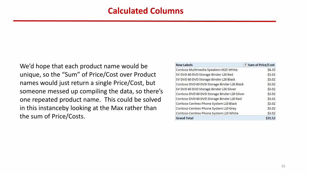
We’d hope that each product name would be unique, so the “Sum” of Price/Cost over Product names would just return a single Price/Cost, but someone messed up compiling the data, so there’s one repeated product name. This could be solved in this instanceby looking at the Max rather than the sum of Price/Costs.

17

Example: Price/lb

Display the top ten priciest items per pound, and how much revenue they generated in Q4 of 2008. Ignore items without weight values provided. (You will need good exception handling, and possibly many calculated columns).

You should start by seeing how many different weights there are and how many different ways they have of describing the same thing. I suggest using nested if statements to come up with appropriate factors, but that’s not the only way to solve the problem.You’ll also need the “iferror” function so you can keep the price/lb columns in numerical format iferror(a, b) calculates a if there’s no error and returns b if a produces an error.

18

Example: Solution

First, create 3 Boolean (true false) columns to handle whether each item weight was in pounds, grams, or ounces using the OR() function

Then create your Price/lb column using the Booleans and nested ifs to choose appropriate factors. I handled errors by hiding them at -$1.

=iferror(if([Inlb?],[UnitPrice]/[Weight],if([InOz?],[UnitPrice]/[Weight]*16,if([InGrams?],[UnitPrice]/[Weight]*453.59,-1))),-1)

19

Example: Solution

You’re now ready to move on to the pivot table. Put Product Names as rows and Max of Price/LB as values and create a top ten filter for product names.

Now add in CalendarYearLabel and CalendarQuarterLabel as rows and Sum of SalesAmount as values, and filter the former 2 to show the appropriate results.

20

Conclusions & Lessons Learned

Students should now be able to use Power Pivot to run basic analysis of data presented in linked tables. They should continue with modules 7-3 and 7-4 to complete our basic tutorials in Power BI.

Students may wish to refer to http://www.microsoft.com/en-us/powerBI/solutions/default.aspx to see demos for how the Power BI suite is used in various business applications, including: Finance HR Marketing Operations and Logistics.