1

Unit 9. Factor markets

Learning objectives:

to apply the concepts of supply and demand to markets for factors;

to analyze the concept of derived demand;

to understand how a factor’s marginal product and the marginal

revenue product affect the demand for the factor;

to consider the role of factor prices in the allocation of scarce

resources;

to consider labour supply and wage and employment determination;

to explain effects of deviations from perfect competition in labour

market;

to explain the determination of economic rent and price for capital;

to consider the role of factor prices in distribution of income and the

sources of income inequality in a market economy.

Questions for revision:

Utility maximization: income and substitution effects

Total product and cost curves;

Profit maximization by a competitive firm;

Equilibrium of a competitive market;

Labour input optimization by a perfectly competitive firm;

Profit maximization by a monopoly;

Price discrimination;

Government regulation of a competitive market.

9.1. Labour supply

Labour supply depends on decisions of working individuals, how

many hours to work (L). The key issue here is a tradeoff between earning

money and enjoing free time (H). Leisure is treated as a good now. In this

sense labour is a bad because working for an hour a person gives up an

hour of enjoing free time.

Decision-making of a working individual is similar to the choise of

a consumer. In this case utility of an individual depends not only on

consumption of commodities but on her leisure time as well: U(C,H),

where

are consumer’s expenditures in fixed prices of a

base period.

2

A worker seeks to maximize utility subject to two constraints:

temporary constraint L+H=T, where T=24 is the daily temporal fund of an

individual and a monetary constraint , where is a non-

labour income of an individual, w is an hourly wage rate, p is the consumer

price index

. So taking into consideration the definition of C

it is easy to see that

are

actual consumer’s expenditures.

Putting the temporal and monetary constraints together one can

write down a composite constraint:

, or

. The real wage rate appears to be an

opportunity cost of leisure.

Optimal individual choise is similar to that of a consumer in

commodity markets. Marginal rate of substitution of consumption and

leisure is equal to real wage rate:

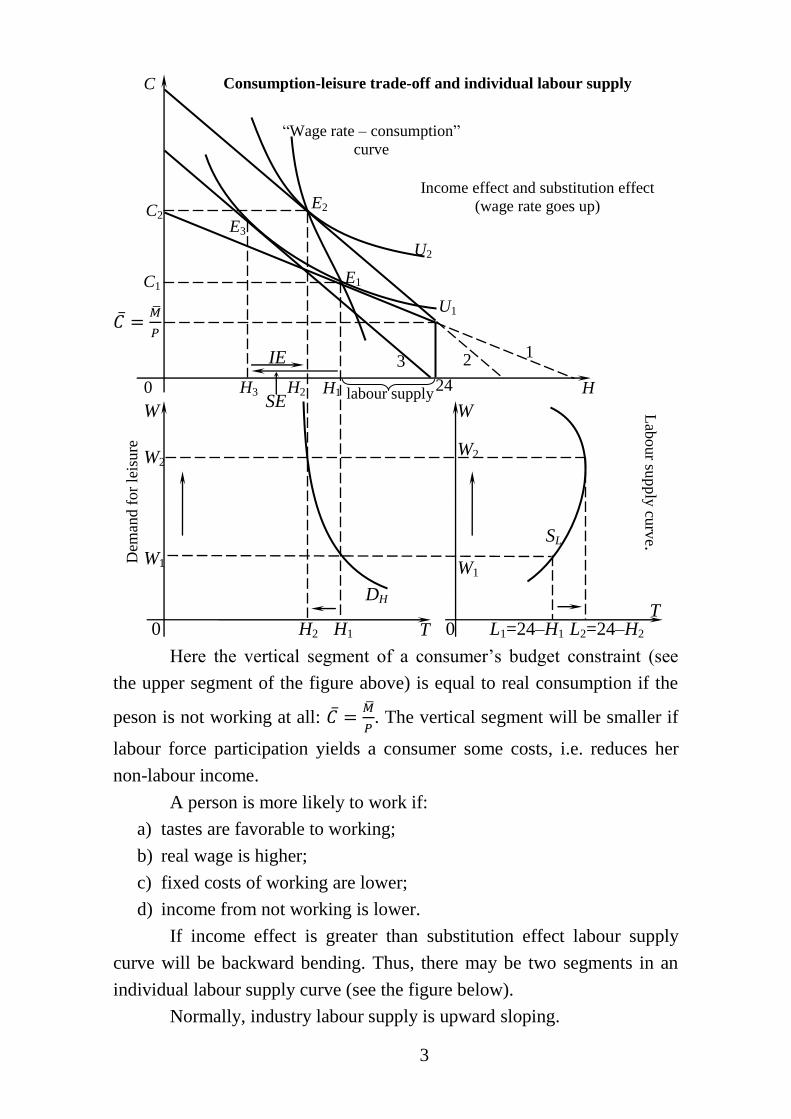
Suppose that the wage rate goes up to consider income and

substitution effects. Labour supply curve (L=24-H) will be upwarg bending

if substitution effect overweights income effect (see the figure below).

3

Here the vertical segment of a consumer’s budget constraint (see

the upper segment of the figure above) is equal to real consumption if the

peson is not working at all:

. The vertical segment will be smaller if

labour force participation yields a consumer some costs, i.e. reduces her

non-labour income.

A person is more likely to work if:

a) tastes are favorable to working;

b) real wage is higher;

c) fixed costs of working are lower;

d) income from not working is lower.

If income effect is greater than substitution effect labour supply

curve will be backward bending. Thus, there may be two segments in an

individual labour supply curve (see the figure below).

Normally, industry labour supply is upward sloping.

C

labour supply 0 H

H2 H1

C2

U2

U1

E1

E2

E3

C1

H3 24

H2 0 0 L1=24–H1 L2=24–H2

W1

W2

T

SL

W

H1

W1

W2

DH

W

T

1 2 3

SE

IE

“Wage rate – consumption”

curve L

abour su

pply

curv

e.

Income effect and substitution effect

(wage rate goes up)

Dem

and f

or

leis

ure

Consumption-leisure trade-off and individual labour supply

4

9.2. Derived demand for factors of production. Marginal revenue

product and marginal factor cost: profit maximization

Recall that a firm is an institution that puts together factor and

product markets (see the first figure in unit 5). In this sense a firm’s

demand for production factors – labour and capital – is a derived demand

as it depends on the demand and consequently the price for the product of

the firm which is sold at product markets markets.

Let’s consider profit maximization in short run, when labour is the

only variable production factor, so labour costs (wL) are variable, and

capital costs (rK) are fixed (FC): . A firm is maximizing

profit with respect to labour factor:

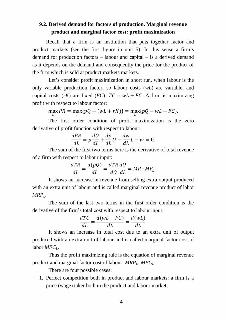
The first order condition of profit maximization is the zero

derivative of profit function with respect to labour:

The sum of the first two terms here is the derivative of total revenue

of a firm with respect to labour input:

It shows an increase in revenue from selling extra output produced

with an extra unit of labour and is called marginal revenue product of labor

MRPL.

The sum of the last two terms in the first order condition is the

derivative of the firm’s total cost with respect to labour input:

It shows an increase in total cost due to an extra unit of output

produced with an extra unit of labour and is called marginal factor cost of

labor MFCL.

Thus the profit maximizing rule is the equation of marginal revenue

product and marginal factor cost of labour: MRPL=MFCL.

There are four possible cases:

1. Perfect competition both in product and labour markets: a firm is a

price (wage) taker both in the product and labour market;

5

2. Imperfect competition in product market and perfect competition in

labour market: a firm possesses market power in a product market

but is a wage taker in labour market;

3. Perfect competition in product market and monopsony in labour

market: a firm is a price taker in product market but faces upward

sloping labour supply curve (can get more labour only by offering

higher wage);

4. Imperfect competition both in product and labour markets: a firm

possesses market power both in the product and labour market.

9.3. Perfect competition at output and labour markets: marginal value

product of labour and a firm’s demand for labour. The demand curve

for labour of a perfectly competitive industry. Equilibrium in labour

market

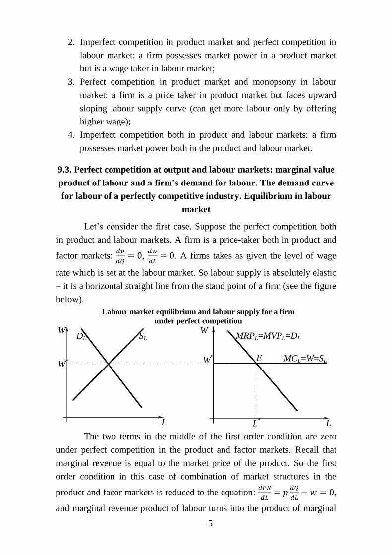
Let’s consider the first case. Suppose the perfect competition both

in product and labour markets. A firm is a price-taker both in product and

factor markets:

,

. A firms takes as given the level of wage

rate which is set at the labour market. So labour supply is absolutely elastic

– it is a horizontal straight line from the stand point of a firm (see the figure

below).

The two terms in the middle of the first order condition are zero

under perfect competition in the product and factor markets. Recall that

marginal revenue is equal to the market price of the product. So the first

order condition in this case of combination of market structures in the

product and facor markets is reduced to the equation:

,

and marginal revenue product of labour turns into the product of marginal

Labour market equilibrium and labour supply for a firm

under perfect competition

E

DL SL W

W* MCL=W=SL

L L* L

W*

W MRPL=MVPL=DL

6

product of labour and the market price for the firm’s output

which is

called marginal value product of labor (MVPL=p·MPL).

So MRPL=VMPL under perfect competition at the product market. If

the labour market is perfectly competitive, MCL=ACL=w, where ACL is a

per unit labour input cost, which is equal to the market price of labour –

wage rate. It follows that under perfect competition both at the product and

labour market a firm will hire labour until the wage rate, which is set at the

labour market, is equal to the marginal value product of labour:

, and a firm’s demand for labour is given by the marginal

value product of labour curve. Summing up: under perfect competition both

at the product and labour market a firm is maximizing profit according to

the rule: w=ACL=MCL=MRPL=MVPL.

The second order condition of profit maximization is the following:

. As the market price is positive (p>0), the derivative of

the marginal product of labour is to be negative:

, so the

law of diminishing marginal product of labour must hold (see the figure

below).

7

Factors of a firm’s demand for labour in short run are the following:

- A change in a wage rate (a shift along the demand for labour curve at

the figure below);

0

w2

w1

L2 L1

DL

L

w Wage rate as a factor of demand for

labour of a competitive firm

L

MPL,

VMPL,

APL,

ARL,

MCL

L

0

MCL

0

TRL

VMPL

ARL

Q,

TR,

TC,

PR

w*

L0

L0

L*

L*

TCL

APL

PR

Labour input optimization by a competitive firm

TPL

MPL

8

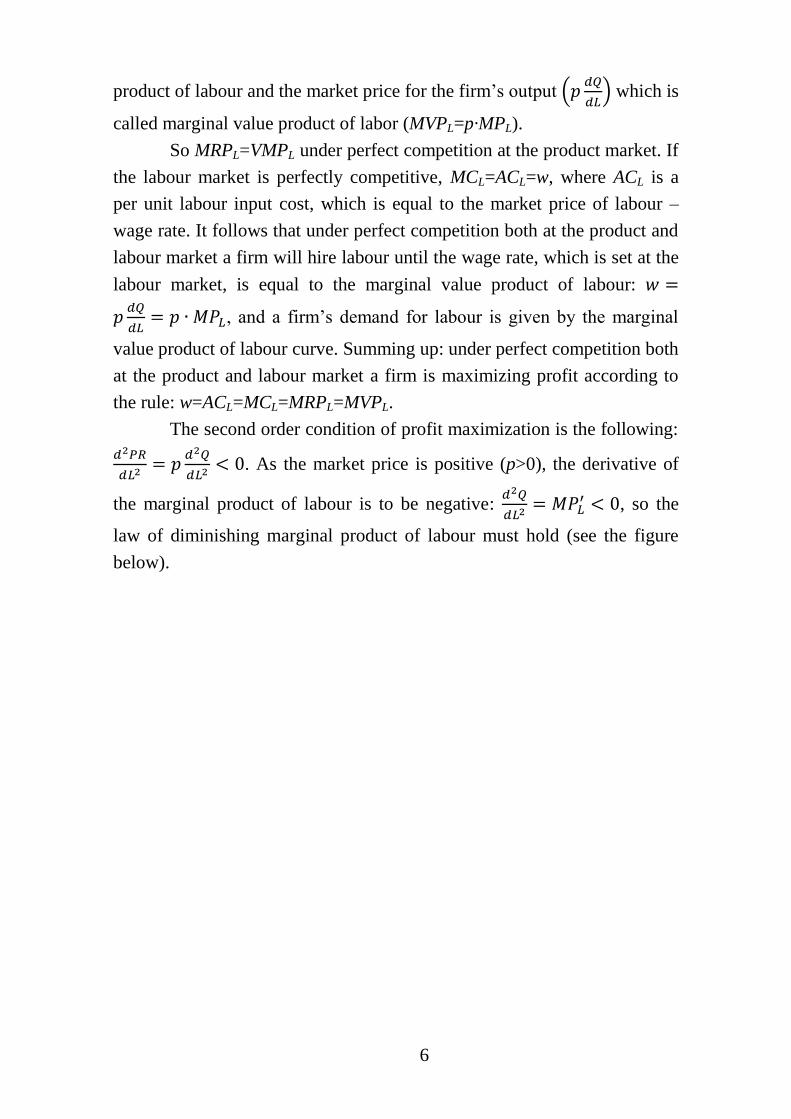
- A change in the demand for the firm’s product (a shift of the demand

for labour curve at the figure below);

- A change in technology, i.e. marginal labour productivity (a shift of

the demand for labour curve at the figure below).

One should note that an industry demand for labour curve is not just

a horizontal sum of demand curves (MVPL) for individual firms. To obtain

the industry demand for labour curve:

- Sum up demand for labour curves (MVPLs) of all the firms in the

industry at given output price p1 (DL(p1) at the figure below);

- Take into consideration a change in output price at the product

market (from p1 to p2 at the figure below) due to a change in a firm’s

output as a result of a fall (rise) of a wage rate, i.e. a shift of a firm’s

demand for labour curve;

- Sum up demand for labour curves (MVPLs) of all the firms in the

industry at the new output price p2 (DL(p2) at the figure below).

L1 L2

L 0

w

w*

Labour productivity as a factor of shift of

firm’s demand for labour

0

p2

p1

p Sq

Q

Demand for product as a factor of shift of the firm’s demand for labour

L1 L2

L 0

w

w*

9

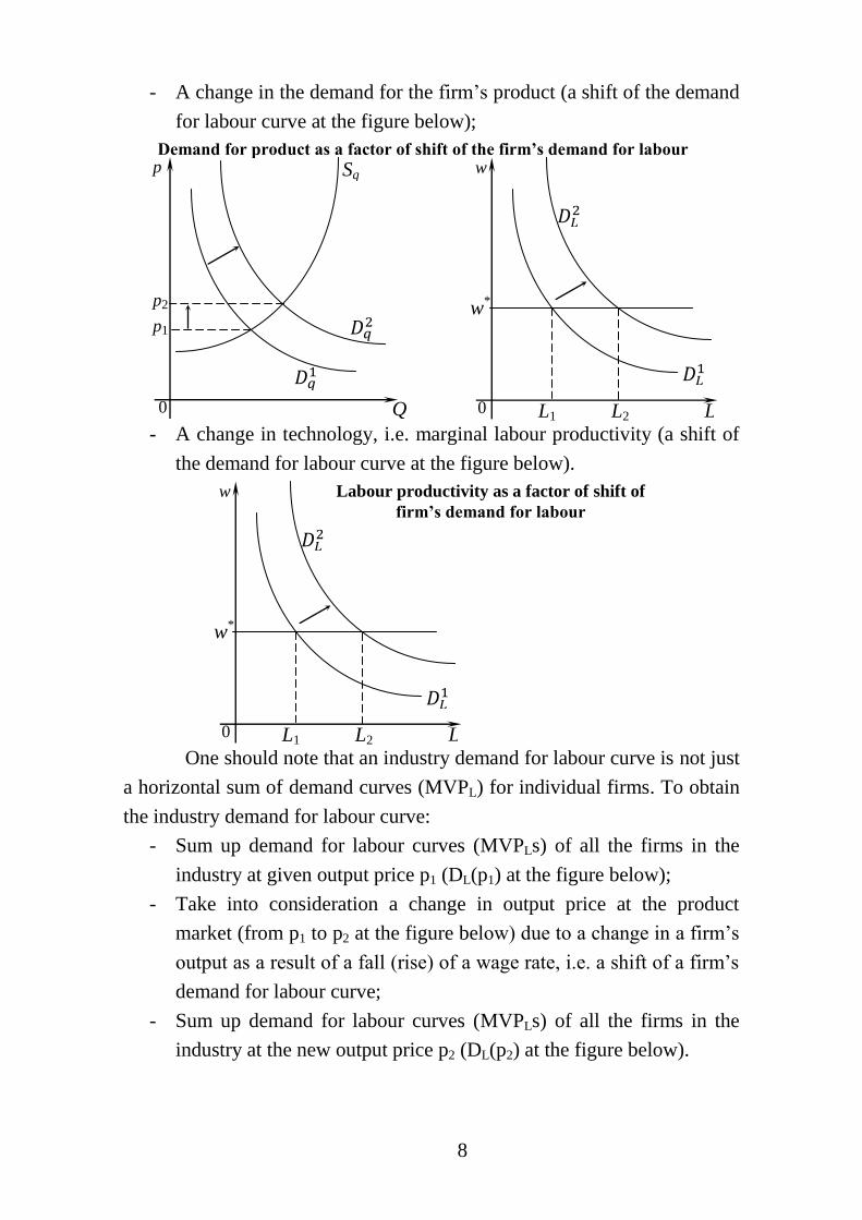
The resulting industry demand for labour curve (DL at the figure

below) will go through initial (w1,L1) and final (w2,L2) equilibrium points

at the industry labour market.

Market demand for labour curve is the horizontal sum of demand

for labou curves of all the industries that hire the given type of labour.

Labour market equilibrium is the point where the market supply of labour

of the given quality and type is equal to market demand for labour.

9.4. Monopoly in product market and perfect competition in labour

market

Let’s now consider the second case: imperfect competition in

product market and perfect competition in labour market. Suppose for

simplicity that the firm is sole producer at the market, i.e. there is a

monopoly. It has market power to influence the price for its product:

.

In this case the first order condition of maximum of profits takes the

form:

So to maximize profits the firm follows labour input optimization

rule: MRPL=MR·MPL=MCL=ACL=w (see the figure below).

Industry demand for labour curve

Q 0

p1

p2

p

S2 S1 D

Product market

L

w2

0 L1 L2 L'

DL(p1)

DL DL(p2)

w

w1

Labour market

10

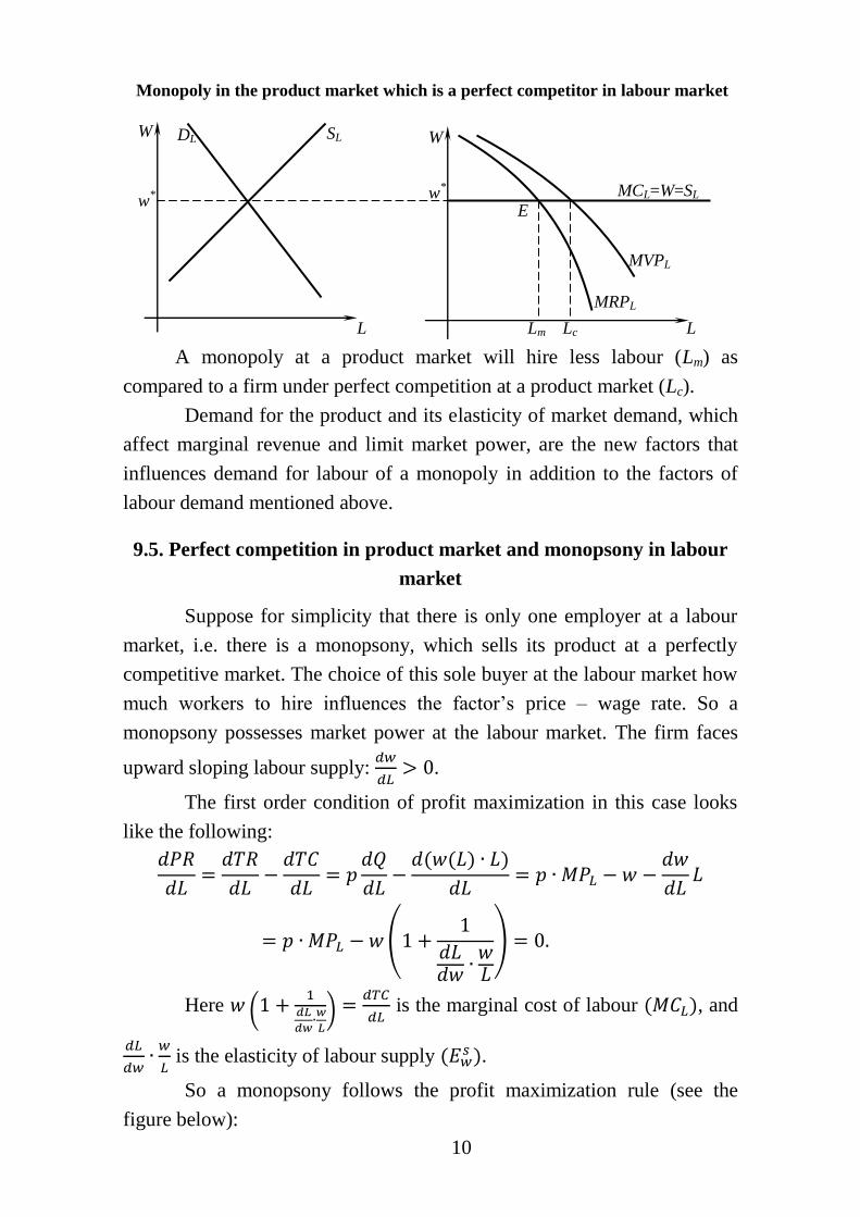
A monopoly at a product market will hire less labour (Lm) as

compared to a firm under perfect competition at a product market (Lc).

Demand for the product and its elasticity of market demand, which

affect marginal revenue and limit market power, are the new factors that

influences demand for labour of a monopoly in addition to the factors of

labour demand mentioned above.

9.5. Perfect competition in product market and monopsony in labour

market

Suppose for simplicity that there is only one employer at a labour

market, i.e. there is a monopsony, which sells its product at a perfectly

competitive market. The choice of this sole buyer at the labour market how

much workers to hire influences the factor’s price – wage rate. So a

monopsony possesses market power at the labour market. The firm faces

upward sloping labour supply:

.

The first order condition of profit maximization in this case looks

like the following:

Here

is the marginal cost of labour , and

is the elasticity of labour supply

.

So a monopsony follows the profit maximization rule (see the

figure below):

DL SL W

L

w*

E w

*

MRPL

MCL=W=SL

Lm L

W

MVPL

Lc

Monopoly in the product market which is a perfect competitor in labour market

11

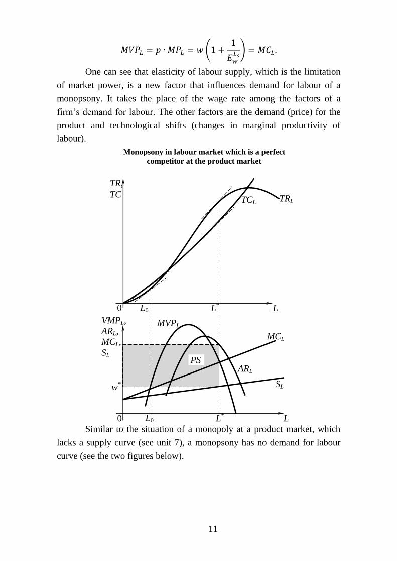
One can see that elasticity of labour supply, which is the limitation

of market power, is a new factor that influences demand for labour of a

monopsony. It takes the place of the wage rate among the factors of a

firm’s demand for labour. The other factors are the demand (price) for the

product and technological shifts (changes in marginal productivity of

labour).

Similar to the situation of a monopoly at a product market, which

lacks a supply curve (see unit 7), a monopsony has no demand for labour

curve (see the two figures below).

L

VMPL,

ARL,

MCL,

SL

L

0

SL

0

TCL

MVPL

ARL

TR,

TC

w*

L0

L0

L*

L*

TRL

MCL

PS

Monopsony in labour market which is a perfect

competitor at the product market

12

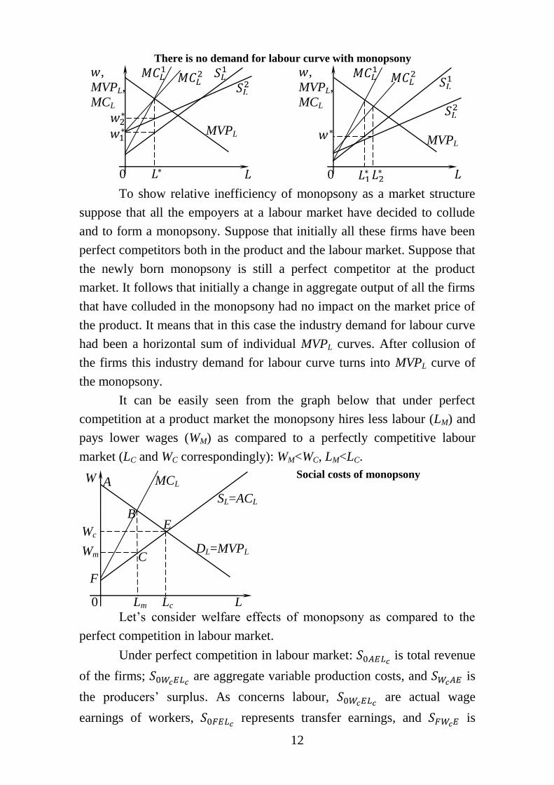
To show relative inefficiency of monopsony as a market structure

suppose that all the empoyers at a labour market have decided to collude

and to form a monopsony. Suppose that initially all these firms have been

perfect competitors both in the product and the labour market. Suppose that

the newly born monopsony is still a perfect competitor at the product

market. It follows that initially a change in aggregate output of all the firms

that have colluded in the monopsony had no impact on the market price of

the product. It means that in this case the industry demand for labour curve

had been a horizontal sum of individual MVPL curves. After collusion of

the firms this industry demand for labour curve turns into MVPL curve of

the monopsony.

It can be easily seen from the graph below that under perfect

competition at a product market the monopsony hires less labour (LM) and

pays lower wages (WM) as compared to a perfectly competitive labour

market (LC and WC correspondingly): WM<WC, LM<LC.

Let’s consider welfare effects of monopsony as compared to the

perfect competition in labour market.

Under perfect competition in labour market: is total revenue

of the firms; are aggregate variable production costs, and is

the producers’ surplus. As concerns labour, are actual wage

earnings of workers, represents transfer earnings, and is

W

SL=ACL

DL=MVPL

L

MCL

Wc

Lc

Wm

Lm 0

Social costs of monopsony A

B

C

E

F

,

MVPL,

MCL

0

MVPL

,

MVPL,

MCL

0

MVPL

There is no demand for labour curve with monopsony

13

workers’ rent. The transfer earnings of a factor of production are minimum

payments required to induce that factor to work in that job. Economic rent

is the extra payment a factor receives over and above the transfer earnings.

So shows social welfare under perfect competition in labour market.

Under monopsony: is total revenue of the firm;

are variable production costs; is the producer’s surplus;

shows actual wage earnings of workers; – transfer earnings;

– workers’ rent. is the social welfare.

is the difference between social welfare under perfect

competition and under monopsony. This is welfare loss of a monopsony.

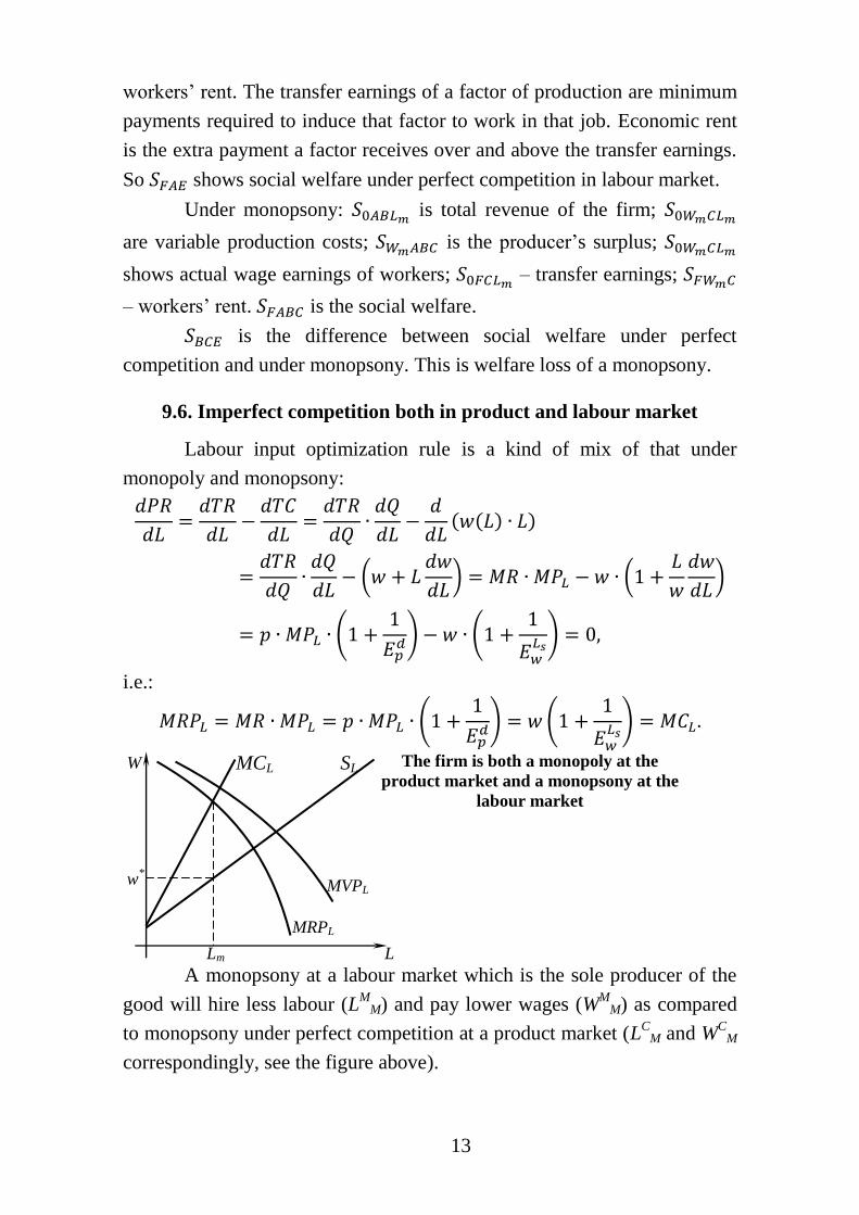
9.6. Imperfect competition both in product and labour market

Labour input optimization rule is a kind of mix of that under

monopoly and monopsony:

i.e.:

A monopsony at a labour market which is the sole producer of the

good will hire less labour (LM

M) and pay lower wages (WM

M) as compared

to monopsony under perfect competition at a product market (LC

M and WC

M

correspondingly, see the figure above).

The firm is both a monopoly at the

product market and a monopsony at the

labour market

SL MCL

w*

MRPL

Lm L

W

MVPL

14

9.7. Demand and supply of capital. Equilibrium in capital market. Net

present value and discounting. Interest rate

Capital markets consist of financial markets and markets for real

assets.

Interest rate is determined at financial markets, where supply of

loanable funds is provided by households (savers) and demand for loanable

funds is required by investors (borrowers).

It is obvious that there is a difference between nominal interest rate

(i) and real interest rate (r): r = i – π, where π is inflation rate. This is the so

called Fisher’s law. Still from now on we shall neglect the differerence

between nominal and real interest rates, i.e. we are going to suppose that

there is no inflation.

Temporal aspect of decision making is one of the most important

factor at the markets for real assets. Value of an asset next year is equal to

(1+r)*PV, where PV is the present value of the asset. It follows that

r

1

yearnext ValueluePresent va . Denote by FV the future value of the asset t

years from now and apply the above consideration t times to get:

FV=PV(1+r)t. Consequently,

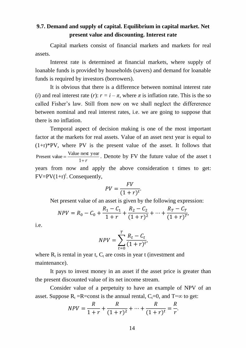
Net present value of an asset is given by the following expression:

i.e.

where Rt is rental in year t, Ct are costs in year t (investment and

maintenance).

It pays to invest money in an asset if the asset price is greater than

the present discounted value of its net income stream.

Consider value of a perpetuity to have an example of NPV of an

asset. Suppose Rt =R=const is the annual rental, Ct=0, and T=∞ to get:

15

Let’s now consider the relationship between asset prices, rental

payments and interest rates taking into consideration depreciation of assets.

Let PA be price of an asset, R – annual rental, C – annual maintenance

costs, r – real interest rate, δ –depreciation rate. Required rental on capital

is rental payment that would just cover the costs.

Let’s suppose that an entrepreneur borrows to invest in projects that

would yield return in future. In this case interest rate is the price of

borrowing for investors. Investment in real and financial assets should yield

at least the same return: R – C + (1 - δ)PA ⩾ PA(1 + r). This gives the

equilibrium price of an asset:

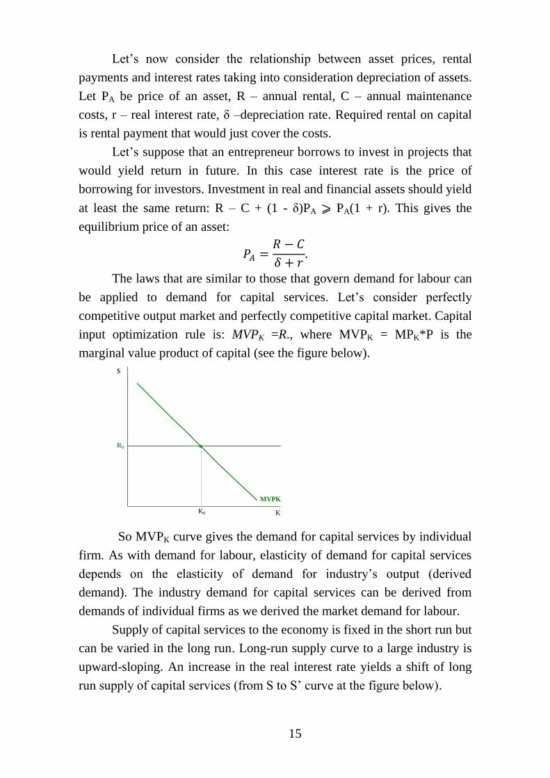
The laws that are similar to those that govern demand for labour can

be applied to demand for capital services. Let’s consider perfectly

competitive output market and perfectly competitive capital market. Capital

input optimization rule is: MVPK =R., where MVPK = MPK*P is the

marginal value product of capital (see the figure below).

So MVPK curve gives the demand for capital services by individual

firm. As with demand for labour, elasticity of demand for capital services

depends on the elasticity of demand for industry’s output (derived

demand). The industry demand for capital services can be derived from

demands of individual firms as we derived the market demand for labour.

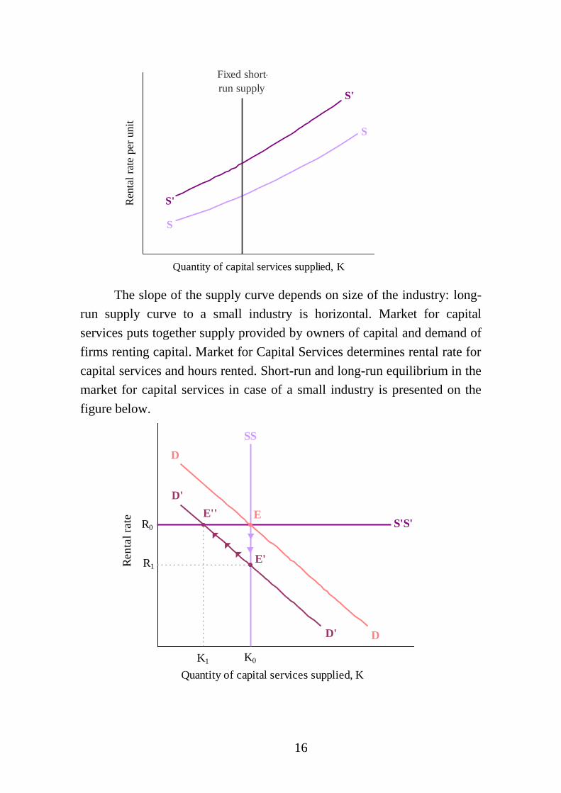
Supply of capital services to the economy is fixed in the short run but

can be varied in the long run. Long-run supply curve to a large industry is

upward-sloping. An increase in the real interest rate yields a shift of long

run supply of capital services (from S to S’ curve at the figure below).

R0

K0

MVPK

$

K

16

The slope of the supply curve depends on size of the industry: long-

run supply curve to a small industry is horizontal. Market for capital

services puts together supply provided by owners of capital and demand of

firms renting capital. Market for Capital Services determines rental rate for

capital services and hours rented. Short-run and long-run equilibrium in the

market for capital services in case of a small industry is presented on the

figure below.

S

S'

S'

Fixed short-

run supply

S

Quantity of capital services supplied, K

Ren

tal

rate

per

unit

S'S'

K1

SS

K0

z

zq

z q

D

DD'

D'

E

E'

E''R0

R1

Quantity of capital services supplied, K

Ren

tal

rate

17

9.8. Wage differentials: discrimination and human capital

Compensating wage differentials is the difference in the wage rate

that reflects attractiveness of a job’s working conditions. Discrimination

means different treatment of people whose relevant characteristics are

identical.

Investment in human capital is another source of wage differentials.

Human capital is the stock of knowledge and skills accumulated by a

worker to enhance future productivity. Investment in human capital may

take the form of:

- education;

- training and on-the-job training;

- experience.

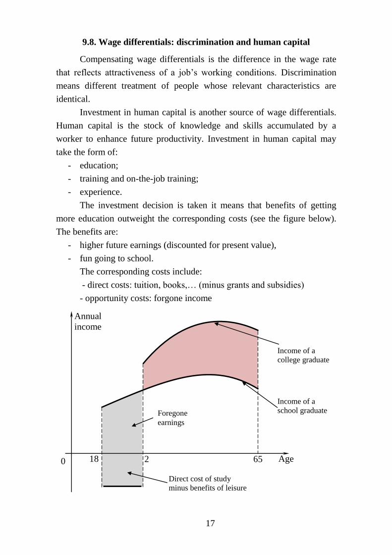
The investment decision is taken it means that benefits of getting

more education outweight the corresponding costs (see the figure below).

The benefits are:

- higher future earnings (discounted for present value),

- fun going to school.

The corresponding costs include:

- direct costs: tuition, books,… (minus grants and subsidies)

- opportunity costs: forgone income

Annual

income

Income of a

college graduate

Income of a

school graduate

18 2

3 Direct cost of study

minus benefits of leisure

Foregone

earnings

65 Age 0