unit- ii ac circuit analysis year/ec t35-ct/unit 2.pdf · unit- ii. ac circuit analysis. series ......

EC T35/CIRCUIT THEORY

13

UNIT- II

AC CIRCUIT ANALYSIS

Series circuits - RC, RL and RLC circuits and Parallel circuits –RLC circuits - Sinusoidal steady state

response - Mesh and Nodal analysis - Analysis of circuits using Superposition, Thevenin’s, Norton’s

and Maximum power transfer theorems. Resonance - Series resonance - Parallel resonance -

Variation of impedance with frequency - Variation in current through and voltage across L and C with

frequency – Bandwidth - Q factor -Selectivity.

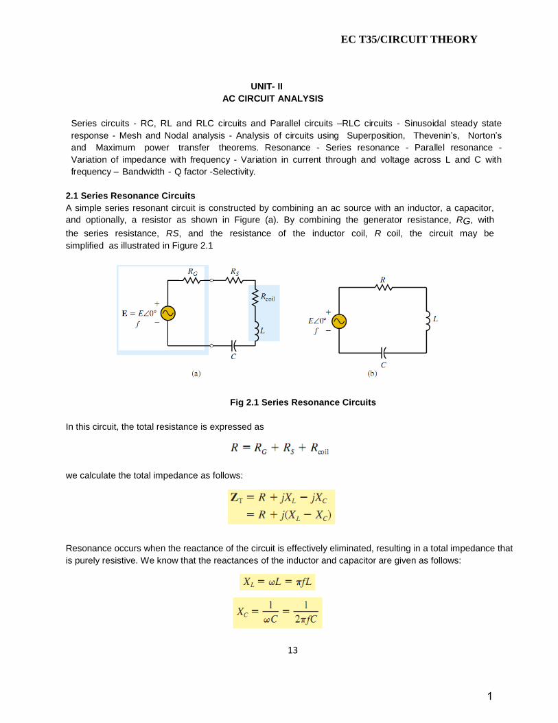
2.1 Series Resonance Circuits

A simple series resonant circuit is constructed by combining an ac source with an inductor, a capacitor,

and optionally, a resistor as shown in Figure (a). By combining the generator resistance, RG, with

the series resistance, RS, and the resistance of the inductor coil, R coil, the circuit may be

simplified as illustrated in Figure 2.1

Fig 2.1 Series Resonance Circuits

In this circuit, the total resistance is expressed as

we calculate the total impedance as follows:

Resonance occurs when the reactance of the circuit is effectively eliminated, resulting in a total impedance that

is purely resistive. We know that the reactances of the inductor and capacitor are given as follows:

1


14

The total impedance of the series circuit at resonance is equal to the total circuit resistance, R. Hence, at

resonance,

Let

The resonant frequency as

The subscript s in the above equations indicates that the frequency determined is the series resonant frequency.

At resonance, the total current in the circuit is determined from Ohm’s law as

2.2 Quality Factor, Q

For any resonant circuit, we define the quality factor, Q, as the ratio of reactive power to average power,

namely,

Because the reactive power of the inductor is equal to the reactive power of the capacitor at resonance,

we may express Q in terms of either reactive power. Consequently, the above expression is written as

follows:

Quite often, the inductor of a given circuit will have a Q expressed in terms of its reactance and internal

resistance, as follows:

2


15

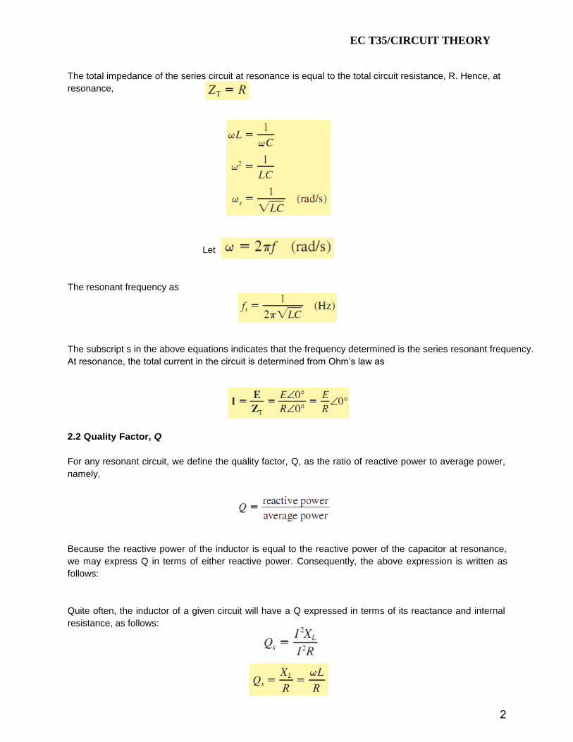
Problem 1

Find the indicated quantities for the circuit

Solution

3


16

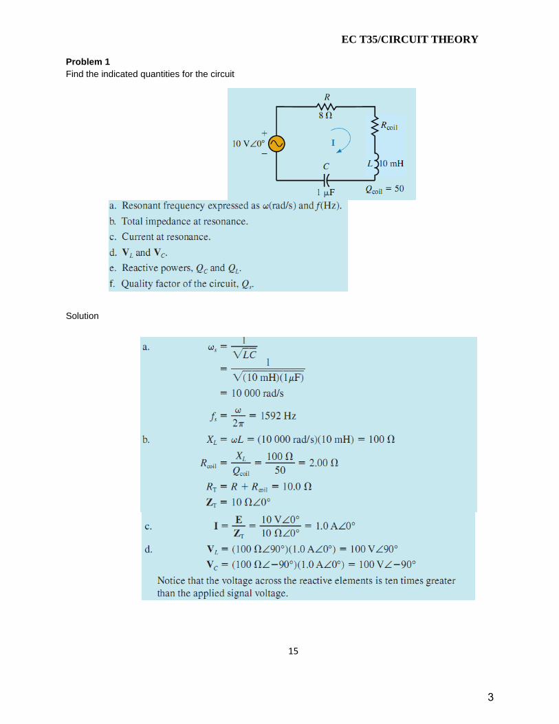
2.3 Impedance of a Series Resonant Circuit

We examine how the impedance of a series resonant circuit varies as a function of frequency. Because

the impedances of inductors and capacitors are dependent upon frequency, the total impedance of a

series resonant circuit must similarly vary with frequency. For algebraic simplicity, we use frequency

The total impedance of a simple series resonant circuit is written as

The magnitude and phase angle of the impedance vector ZT, are expressed as follows:

Examining these equations for various values of frequency, we note that the following conditions will apply:

Fig 2.2 Impedance

4


17

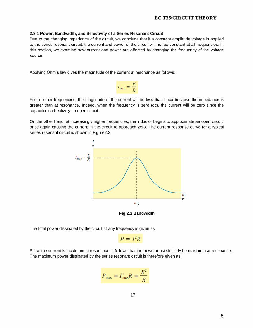
2.3.1 Power, Bandwidth, and Selectivity of a Series Resonant Circuit

Due to the changing impedance of the circuit, we conclude that if a constant amplitude voltage is applied

to the series resonant circuit, the current and power of the circuit will not be constant at all frequencies. In

this section, we examine how current and power are affected by changing the frequency of the voltage

source.

Applying Ohm’s law gives the magnitude of the current at resonance as follows:

For all other frequencies, the magnitude of the current will be less than Imax because the impedance is

greater than at resonance. Indeed, when the frequency is zero (dc), the current will be zero since the

capacitor is effectively an open circuit.

On the other hand, at increasingly higher frequencies, the inductor begins to approximate an open circuit,

once again causing the current in the circuit to approach zero. The current response curve for a typical

series resonant circuit is shown in Figure2.3

Fig 2.3 Bandwidth

The total power dissipated by the circuit at any frequency is given as

Since the current is maximum at resonance, it follows that the power must similarly be maximum at resonance.

The maximum power dissipated by the series resonant circuit is therefore given as

5


18

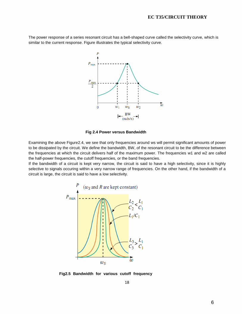
The power response of a series resonant circuit has a bell-shaped curve called the selectivity curve, which is

similar to the current response. Figure illustrates the typical selectivity curve.

Fig 2.4 Power versus Bandwidth

Examining the above Figure2.4, we see that only frequencies around ws will permit significant amounts of power

to be dissipated by the circuit. We define the bandwidth, BW, of the resonant circuit to be the difference between

the frequencies at which the circuit delivers half of the maximum power. The frequencies w1 and w2 are called

the half-power frequencies, the cutoff frequencies, or the band frequencies.

If the bandwidth of a circuit is kept very narrow, the circuit is said to have a high selectivity, since it is highly

selective to signals occuring within a very narrow range of frequencies. On the other hand, if the bandwidth of a

circuit is large, the circuit is said to have a low selectivity.

Fig2.5 Bandwidth for various cutoff frequency

6


19

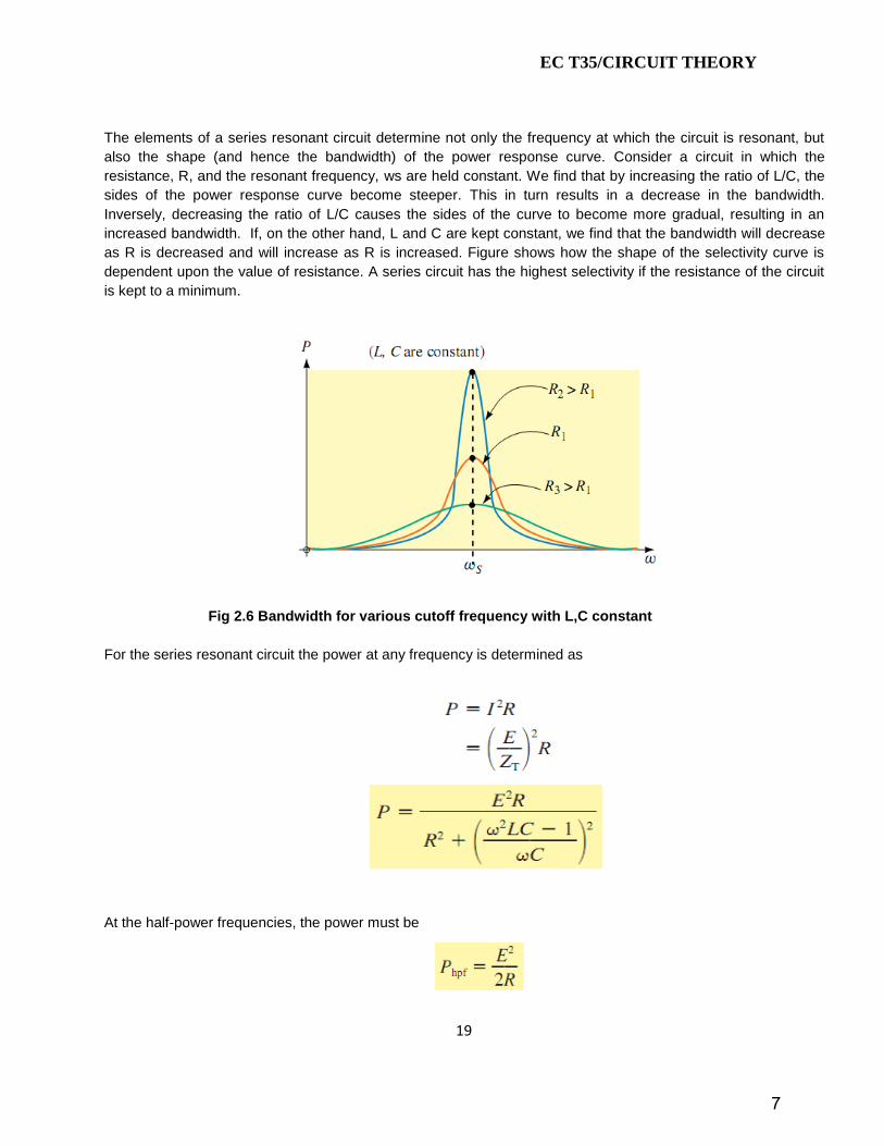
The elements of a series resonant circuit determine not only the frequency at which the circuit is resonant, but

also the shape (and hence the bandwidth) of the power response curve. Consider a circuit in which the

resistance, R, and the resonant frequency, ws are held constant. We find that by increasing the ratio of L/C, the

sides of the power response curve become steeper. This in turn results in a decrease in the bandwidth.

Inversely, decreasing the ratio of L/C causes the sides of the curve to become more gradual, resulting in an

increased bandwidth. If, on the other hand, L and C are kept constant, we find that the bandwidth will decrease

as R is decreased and will increase as R is increased. Figure shows how the shape of the selectivity curve is

dependent upon the value of resistance. A series circuit has the highest selectivity if the resistance of the circuit

is kept to a minimum.

Fig 2.6 Bandwidth for various cutoff frequency with L,C constant

For the series resonant circuit the power at any frequency is determined as

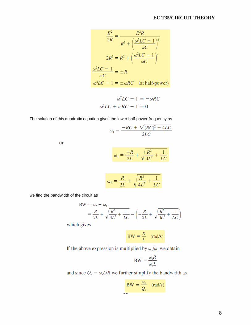
At the half-power frequencies, the power must be

7


20

The solution of this quadratic equation gives the lower half-power frequency as

we find the bandwidth of the circuit as

8


21

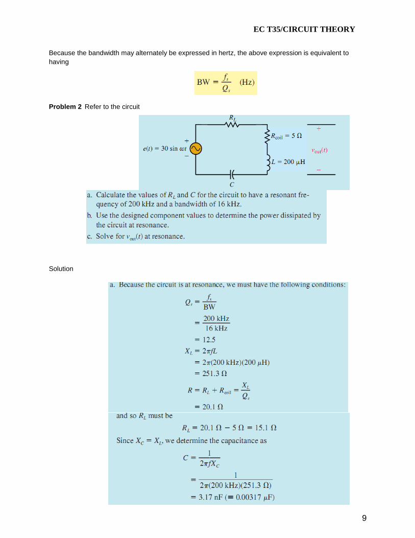
Because the bandwidth may alternately be expressed in hertz, the above expression is equivalent to

having

Problem 2 Refer to the circuit

Solution

9


22

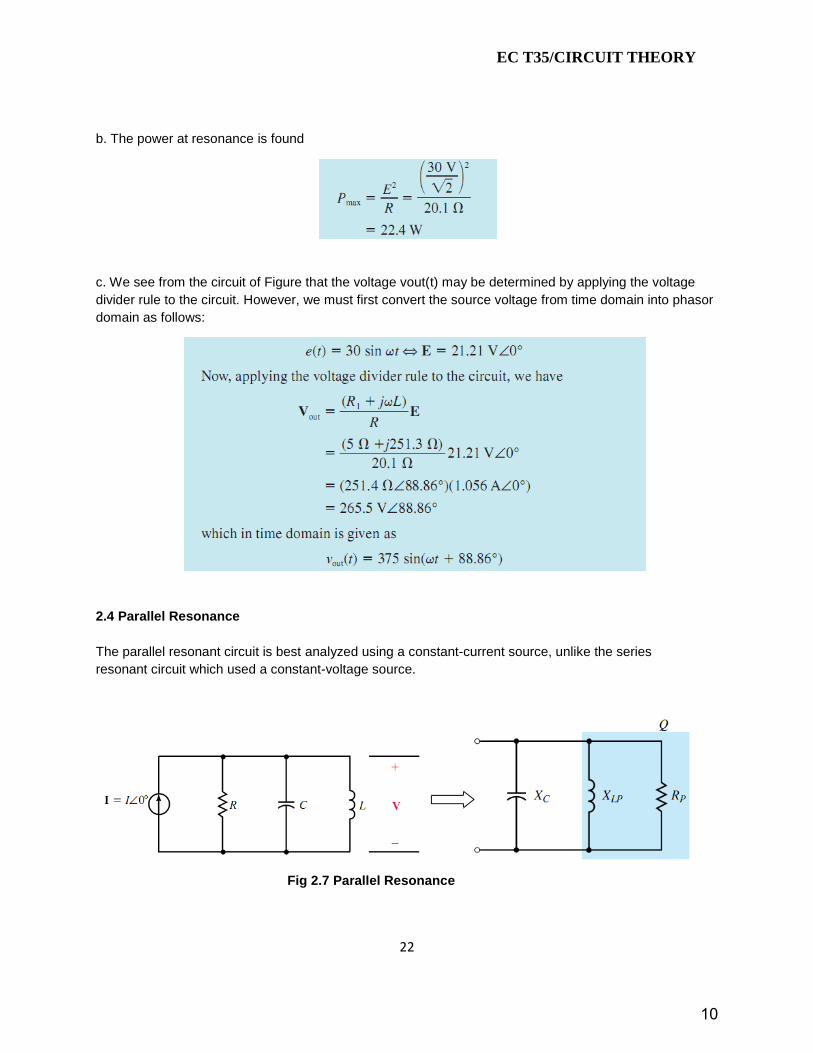
b. The power at resonance is found

c. We see from the circuit of Figure that the voltage vout(t) may be determined by applying the voltage

divider rule to the circuit. However, we must first convert the source voltage from time domain into phasor

domain as follows:

2.4 Parallel Resonance

The parallel resonant circuit is best analyzed using a constant-current source, unlike the series

resonant circuit which used a constant-voltage source.

Fig 2.7 Parallel Resonance

10


23

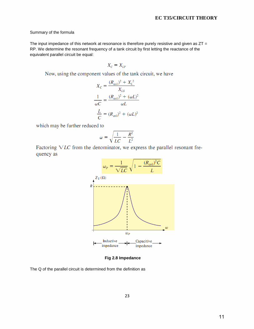
Summary of the formula

The input impedance of this network at resonance is therefore purely resistive and given as ZT =

RP. We determine the resonant frequency of a tank circuit by first letting the reactance of the

equivalent parallel circuit be equal:

Fig 2.8 Impedance

The Q of the parallel circuit is determined from the definition as

11


24

The bandwidth is therefore

Problem 2

Consider the

circuit

12


25

Solution

The half-power frequencies

13


26

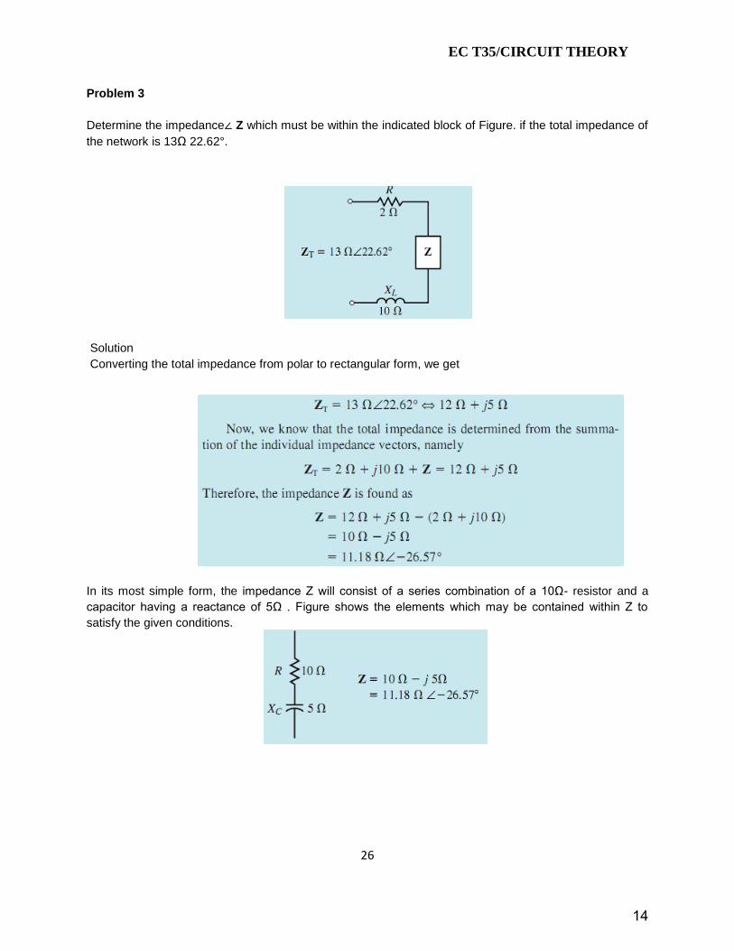
Problem 3

Determine the impedance∠ Z which must be within the indicated block of Figure. if the total impedance of

the network is 13Ω 22.62°.

Solution

Converting the total impedance from polar to rectangular form, we get

In its most simple form, the impedance Z will consist of a series combination of a 10Ω- resistor and a

capacitor having a reactance of 5Ω . Figure shows the elements which may be contained within Z to

satisfy the given conditions.

14


27

Problem 4

Refer to the circuit

a. Find the impedance Z

b. Calculate the power factor of the circuit.

c. Determine I.

d. Sketch the phasor diagram for E and I.

e. Find the average power delivered to the circuit by the voltage source.

Calculate the average power dissipated by both the resistor and the capacitor

Solution

The phasor diagram is

From this phasor diagram, we see that the current phasor for the capacitive circuit leads the

voltage phasor by 53.13°.

15


28

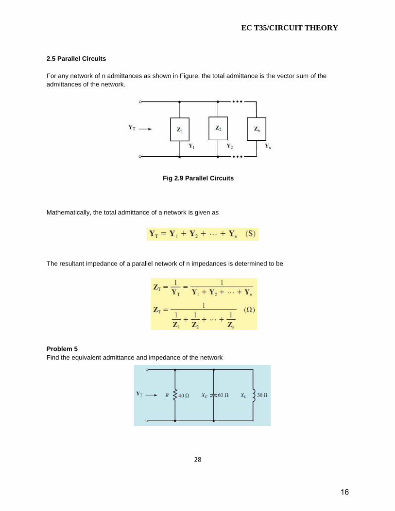
2.5 Parallel Circuits

For any network of n admittances as shown in Figure, the total admittance is the vector sum of the

admittances of the network.

Fig 2.9 Parallel Circuits

Mathematically, the total admittance of a network is given as

The resultant impedance of a parallel network of n impedances is determined to be

Problem 5

Find the equivalent admittance and impedance of the network

16


29

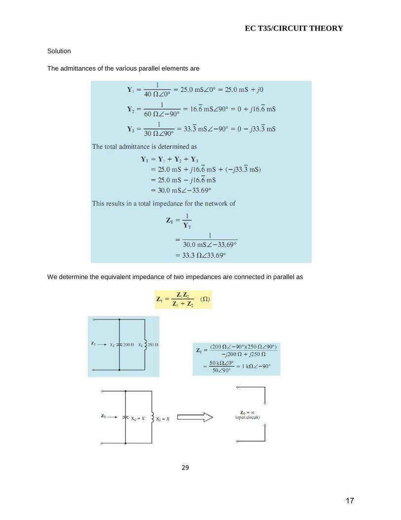
Solution

The admittances of the various parallel elements are

We determine the equivalent impedance of two impedances are connected in parallel as

17


30

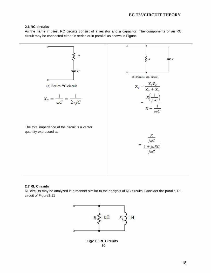
2.6 RC circuits

As the name implies, RC circuits consist of a resistor and a capacitor. The components of an RC

circuit may be connected either in series or in parallel as shown in Figure.

The total impedance of the circuit is a vector

quantity expressed as

2.7 RL Circuits

RL circuits may be analyzed in a manner similar to the analysis of RC circuits. Consider the parallel RL

circuit of Figure2.11

Fig2.10 RL Circuits

18


31

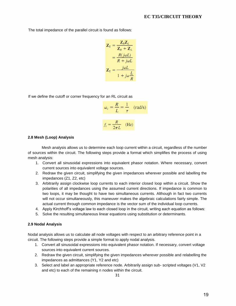
The total impedance of the parallel circuit is found as follows:

If we define the cutoff or corner frequency for an RL circuit as

2.8 Mesh (Loop) Analysis

Mesh analysis allows us to determine each loop current within a circuit, regardless of the number

of sources within the circuit. The following steps provide a format which simplifies the process of using

mesh analysis:

1. Convert all sinusoidal expressions into equivalent phasor notation. Where necessary, convert

current sources into equivalent voltage sources.

2. Redraw the given circuit, simplifying the given impedances wherever possible and labelling the

impedances (Z1, Z2, etc)

3. Arbitrarily assign clockwise loop currents to each interior closed loop within a circuit. Show the

polarities of all impedances using the assumed current directions. If impedance is common to

two loops, it may be thought to have two simultaneous currents. Although in fact two currents

will not occur simultaneously, this maneuver makes the algebraic calculations fairly simple. The

actual current through common impedance is the vector sum of the individual loop currents.

4. Apply Kirchhoff’s voltage law to each closed loop in the circuit, writing each equation as follows:

5. Solve the resulting simultaneous linear equations using substitution or determinants.

2.9 Nodal Analysis

Nodal analysis allows us to calculate all node voltages with respect to an arbitrary reference point in a

circuit. The following steps provide a simple format to apply nodal analysis.

1. Convert all sinusoidal expressions into equivalent phasor notation. If necessary, convert voltage

sources into equivalent current sources.

2. Redraw the given circuit, simplifying the given impedances wherever possible and relabelling the

impedances as admittances (Y1, Y2 and etc)

3. Select and label an appropriate reference node. Arbitrarily assign sub- scripted voltages (V1, V2

and etc) to each of the remaining n nodes within the circuit.

19


32

4. Indicate assumed current directions through all admittances in the circuit. If an admittance is

common to two nodes, it is considered in each of the two node equations.

5. Apply Kirchhoff’s current law to each of the n nodes in the circuit

2.10 Superposition Theorem

The voltage across (or current through) an element is determined by summing the voltage (or current)

due to each independent source.

Problem 6: Determine the current I in Figure (a) by using the superposition theorem.

Fig (b)

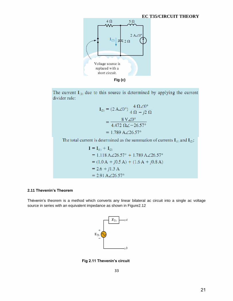
Current due to the 2 A∠0° current source: Eliminating the voltage source, we obtain the circuit shown in

Figure (c).

20


33

Fig (c)

2.11 Thevenin’s Theorem

Thévenin’s theorem is a method which converts any linear bilateral ac circuit into a single ac voltage

source in series with an equivalent impedance as shown in Figure2.12

Fig 2.11 Thevenin’s circuit

21


34

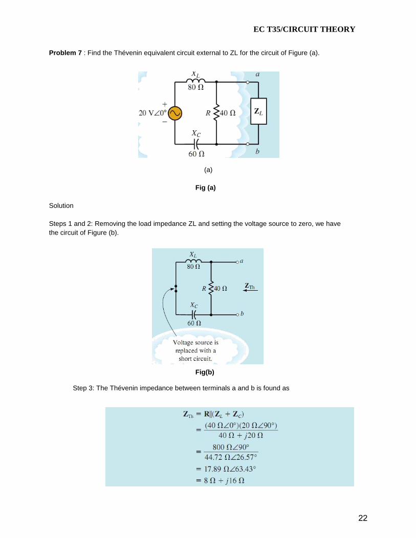
Problem 7 : Find the Thévenin equivalent circuit external to ZL for the circuit of Figure (a).

(a)

Fig (a)

Solution

Steps 1 and 2: Removing the load impedance ZL and setting the voltage source to zero, we have

the circuit of Figure (b).

Fig(b)

Step 3: The Thévenin impedance between terminals a and b is found as

22


35

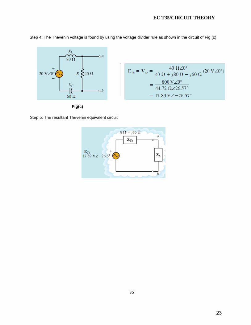
Step 4: The Thevenin voltage is found by using the voltage divider rule as shown in the circuit of Fig (c).

Fig(c)

Step 5: The resultant Thevenin equivalent circuit

23

unit- ii ac circuit analysis year/ec t35-ct/unit 2.pdf · unit- ii. ac circuit analysis. series ......

Documents