unit i:theory of the consumer introduction: what is microeconomics? theory of the consumer...
TRANSCRIPT

UNIT I:Theory of the Consumer
• Introduction: What is Microeconomics?• Theory of the Consumer• Individual & Market Demand
6/25
Theory of the Consumer
• Preferences• Indifference Curves• Utility Functions• Optimization • Income & Substitution Effects
How do they respond to changes in prices and income?
How do consumers make optimal choices?

We said last time that microeconomics is built on the assumption that a rational consumer will attempt to maximize (expected) utility. But what is utility?
Over time, economists have moved away from a notion of cardinal utility (an objective, measurable scale, e.g., height, weight) and toward ordinal utility, built up from a simple binary relation, preference.
Theory of the Consumer

We start by assuming that a rational individual can always compare any 2 alternatives (“consumption bundles” or “market baskets”). We call this basic relationship preference: For any pair of alternatives, A and B, either
A > B A is preferred to B
A < B B is preferred to A
A = B Indifference
Preferences
e.g., 2 apples & 3 oranges.
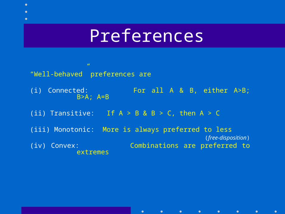
“Well-behaved” preferences are (i) Connected: For all A & B, either A>B; B>A; A=B
(ii) Transitive: If A > B & B > C, then A > C (iii) Monotonic: More is always preferred to less
(free-disposition)
(iv) Convex: Combinations are preferred to extremes
Preferences

Preferences
Y
X
A
B
3
2
2 3
A = ( 2 , 3 )
B = ( 3 , 2 )
A ? B

Preferences
Y
X
A
B
Ya
Yb
Xa Xb
A = (Xa, Ya)
B = (Xb, Yb)
A ? B
Preferences
Y
X
A C
B
Ya
Yb
Xa Xb
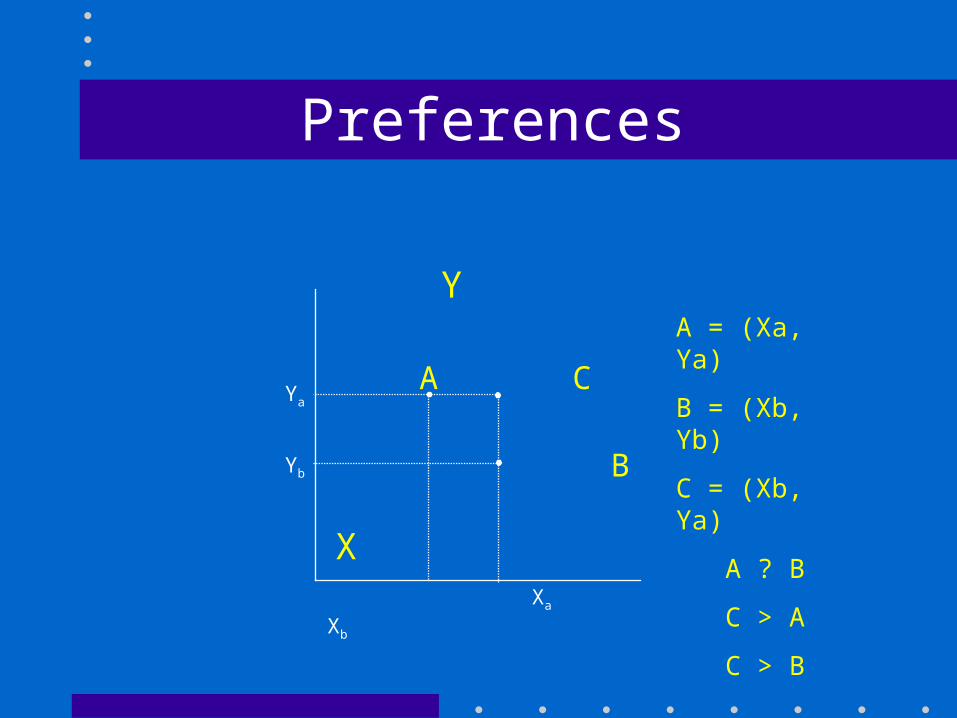
A = (Xa, Ya)
B = (Xb, Yb)
C = (Xb, Ya)
A ? B
C > A
C > B
Preferences
Y
X
A C
B
Ya
Yb
Xa Xb
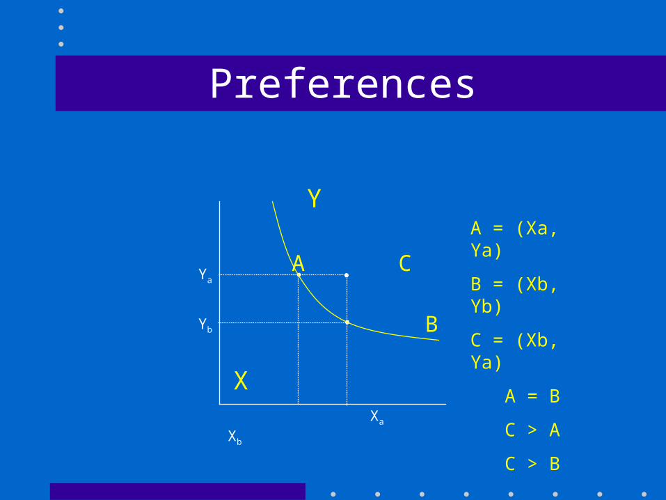
A = (Xa, Ya)
B = (Xb, Yb)
C = (Xb, Ya)
A = B
C > A
C > B

Preferences
Y
X
A C
B
Ya
Yb
Xa Xb
A = (Xa, Ya)
B = (Xb, Yb)
C = (Xb, Ya)
A = B
D > E
D > B
D > A
DE
Convexity

Preferences
Y
X
A C
B
Ya
Yb
Xa Xb
A = (Xa, Ya)
B = (Xb, Yb)
C = (Xb, Ya)
A = B = E
D > E
D > B
D > A
DE
Indifference curves
Indifference Curves
Y
X
3
2
2 3
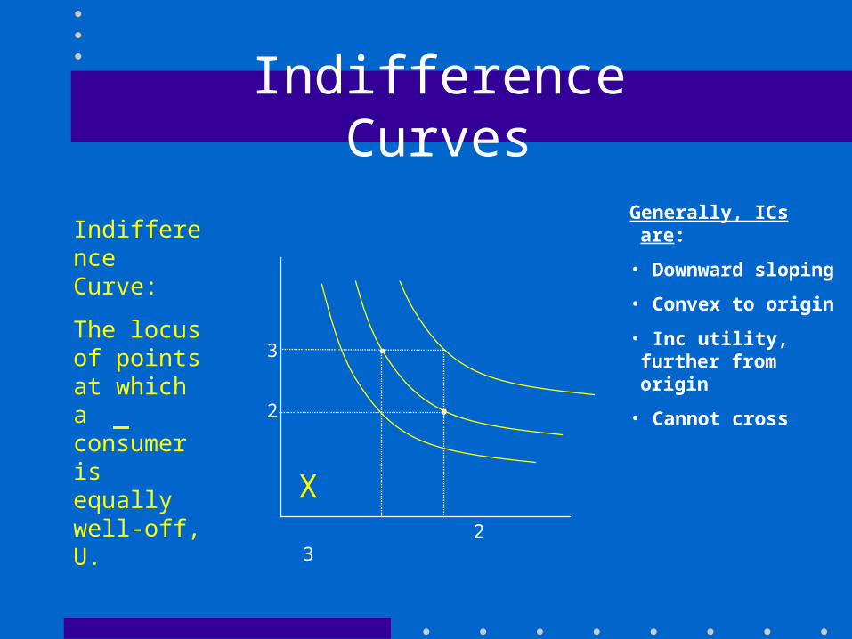
Generally, ICs are:
• Downward sloping
• Convex to origin
• Inc utility, further from origin
• Cannot cross
U = XYIndifference Curve:
The locus of points at which a consumer is equally well-off, U.

Indifference Curves
Y
X
3
2
2 3
Generally, ICs are:
• Downward sloping
• Convex to origin
• Inc utility, further from origin
• Cannot cross
U = 9
U = 6
U = 4
U = XY

Indifference Curves
Y
X
3
2
2 3
Generally, ICs are:
• Downward sloping
• Convex to origin
• Inc utility, further from origin
• Cannot cross
A = B; A = C; B > C !!
U = XY
A
B
C
Indifference Curves
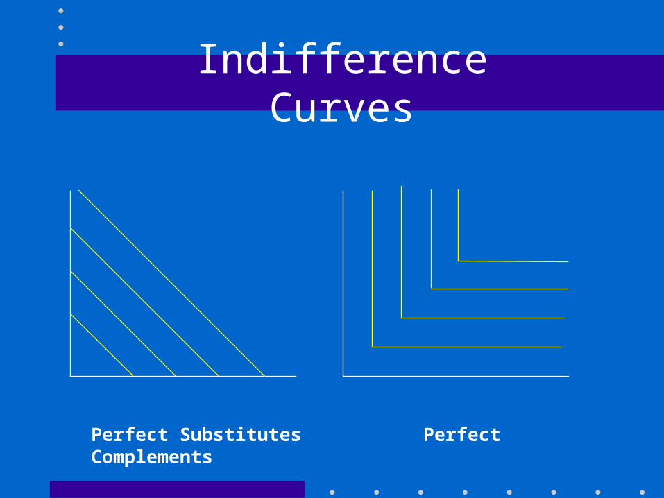
Perfect Substitutes Perfect Complements
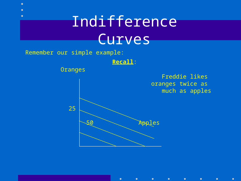
Indifference CurvesRemember our simple example:
Recall: Oranges
Freddie likes oranges twice as
much as apples
25100
50 Apples
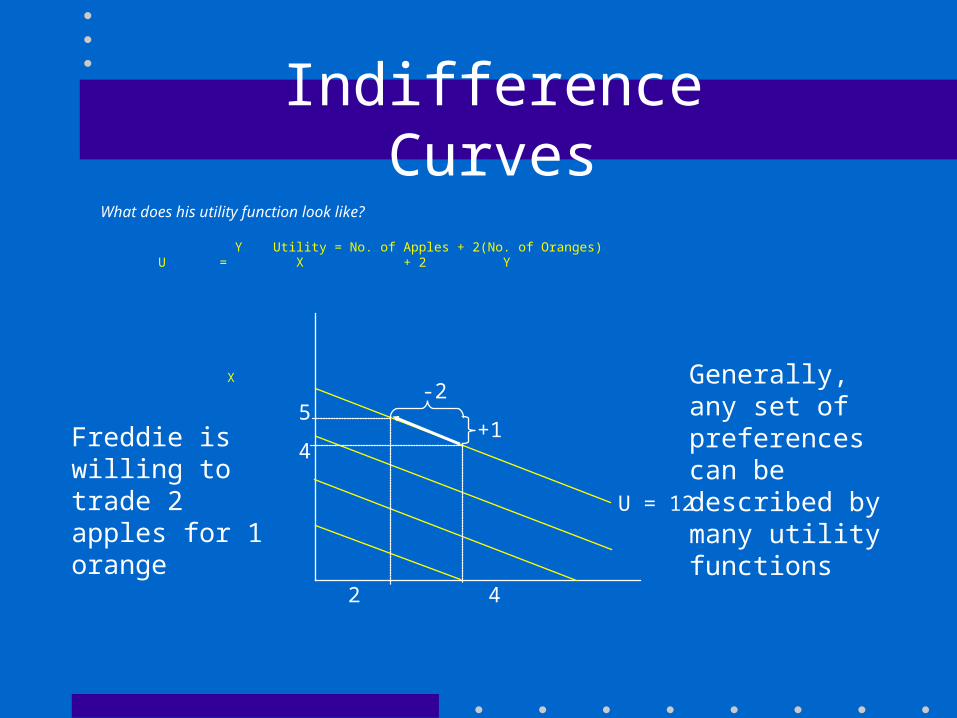
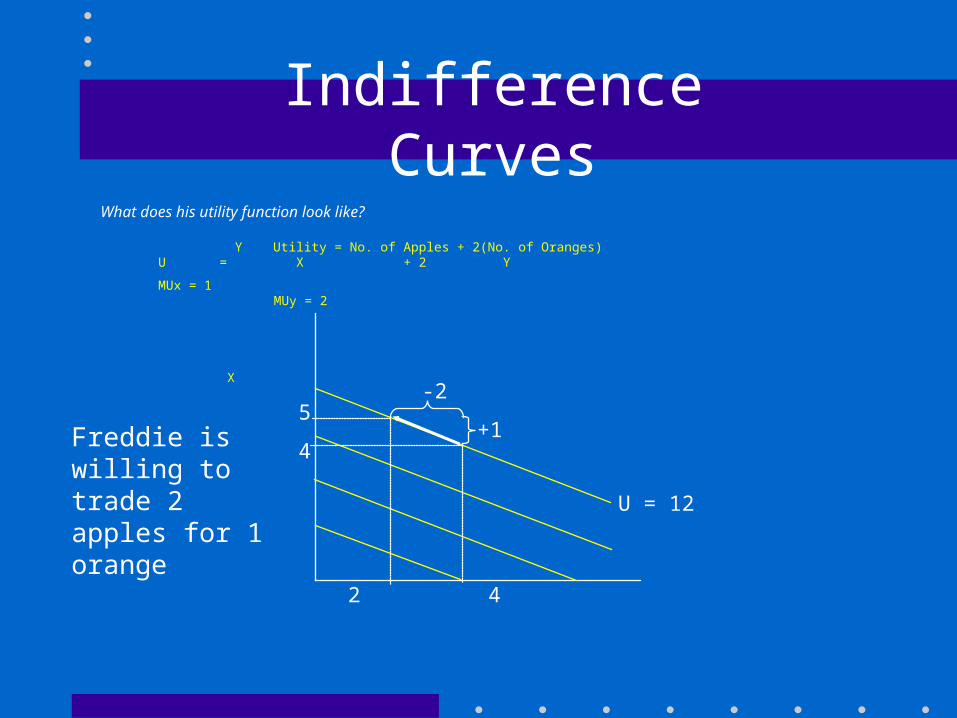
What does his utility function look like?
Y Utility = No. of Apples + 2(No. of Oranges) U = X + 2 Y
MUx = 1 MUy = 2
X
Freddie is willing to trade 2 apples for 1 orange
5
4
2 4
-2
+1
Generally, any set of preferences can be described by many utility functionsU = 12
Indifference Curves
What does his utility function look like?
Y Utility = No. of Apples + 2(No. of Oranges) U = X + 2 Y
MUx = 1 MUy = 2
X
Freddie is willing to trade 2 apples for 1 orange
5
4
2 4
-2
+1
U = 12
Indifference Curves

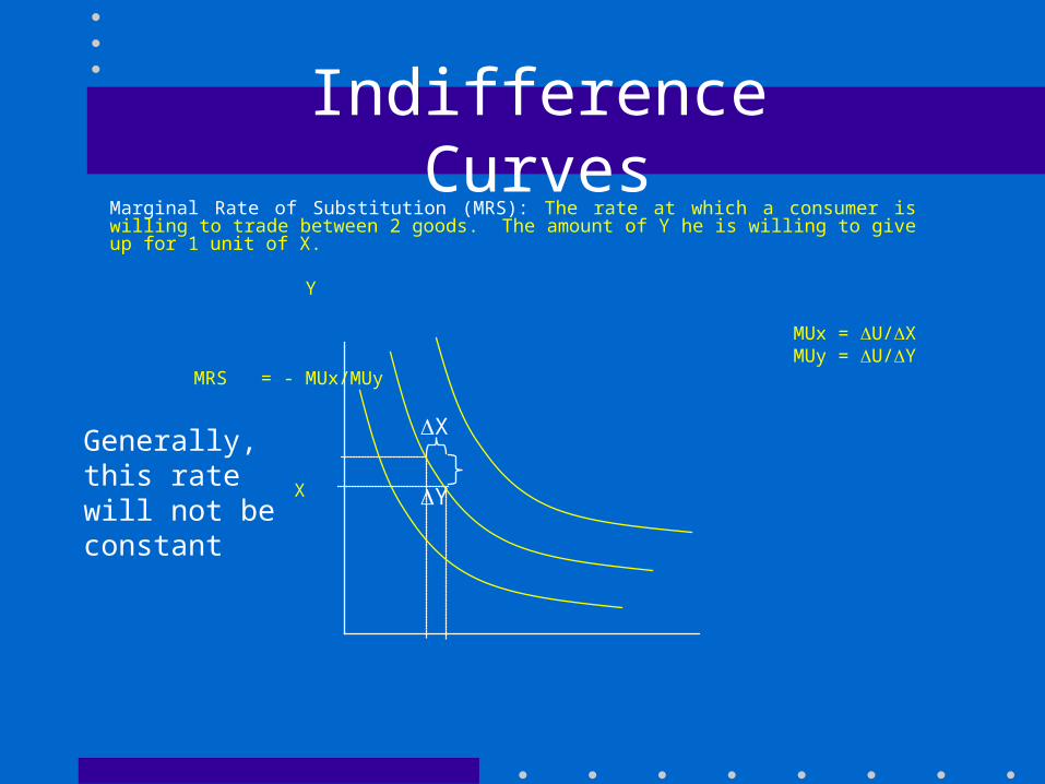
Marginal Rate of Substitution (MRS): The rate at which a consumer is willing to trade between 2 goods. The amount of Y he is willing to give up for 1 unit of X.
Y Utility = No. of Apples + 2(No. of Oranges) U = X + 2 Y
MUx = 1 MUy = 2
MRS = - MUx/MUy = - ½
X
Freddie is willing to trade 2 apples for 1 orange
5
4
2 4
-2
+1
Indifference Curves
Marginal Rate of Substitution (MRS): The rate at which a consumer is willing to trade between 2 goods. The amount of Y he is willing to give up for 1 unit of X.
Y Utility = No. of Apples + 2(No. of Oranges) U = X + 2 Y
MUx = U/X MUy = U/Y
MRS = - MUx/MUy = - ½
X
X
YGenerally, this rate will not be constant; it will depend upon the consumer’s endowment.
Indifference Curves
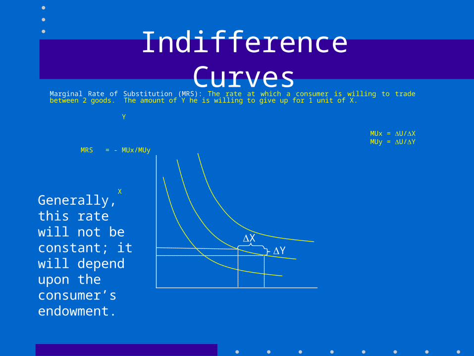
Marginal Rate of Substitution (MRS): The rate at which a consumer is willing to trade between 2 goods. The amount of Y he is willing to give up for 1 unit of X.
Y Utility = No. of Apples + 2(No. of Oranges) U = X + 2 Y
MUx = U/X MUy = U/Y
MRS = - MUx/MUy = - ½
X
Generally, this rate will not be constant; it will depend upon the consumer’s endowment.
XY
Indifference Curves
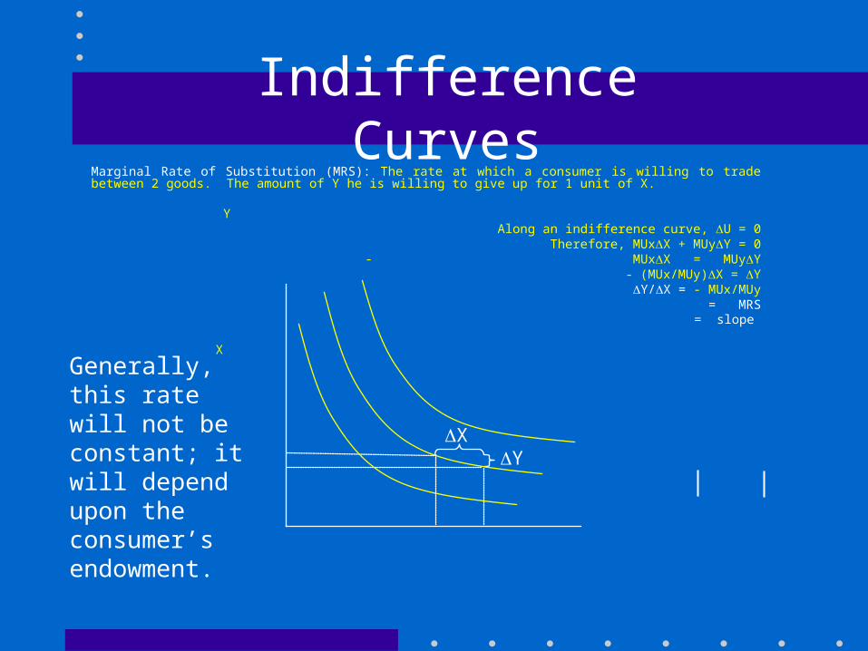
Marginal Rate of Substitution (MRS): The rate at which a consumer is willing to trade between 2 goods. The amount of Y he is willing to give up for 1 unit of X.
Y Utility = No. of Apples + 2(No. of Oranges) U Along an indifference curve, U = 0
Therefore, MUxX + MUyY = 0- MUxX = MUyY
- (MUx/MUy)X = YY/X = - MUx/MUy
= MRS= slope
X
Generally, this rate will not be constant; it will depend upon the consumer’s endowment.
XY
Indifference Curves

Utility Functions
X
U
Assume 1 Good:
U = 2X
Utility: The total amount of satisfaction one enjoys from a given level of consumption (X,Y)

Utility Functions
X
U
Assume 1 Good:
X
U
U = 2X
MUx = U/X
= 2
Marginal Utility: The amount by which utility increases when consumption (of good X) increase by one unit
MUx = U/X
MUx

Utility Functions
XX
U U
Assume 1 Good:
X
U
U
X
U = 2X
MUx = U/X
= 2
U (X)
Diminishing Marginal Utility: Utility increases but at a decreasing rate

Utility Functions
Y
X
U
Now Assume 2 Goods:
U (X)U (Y)
U = f(X,Y)

Utility Functions
Y
X
U
U0 U1 U2 U3
U1
U2
U3
U0
U = f(X,Y)
Indifference curves

Utility Functions
Y
X
U
U0 U1 U2 U3
U1
U2
U3
U0
U = f(X,Y)
XY
MRSyx
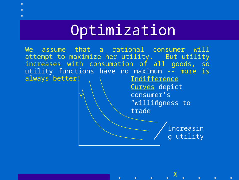
OptimizationWe assume that a rational consumer will attempt to maximize her utility. But utility increases with consumption of all goods, so utility functions have no maximum -- more is always better!
Y Utility = No. of Apples + 2(No. of Oranges)
U
X
Increasing utility
Indifference Curves depict consumer’s “willingness to trade”
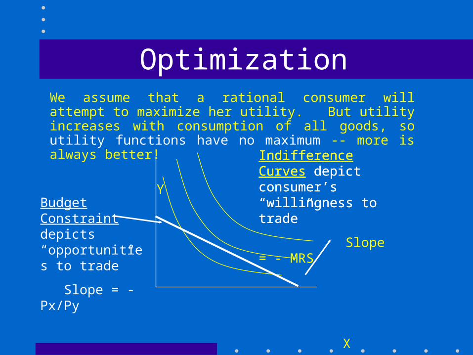
OptimizationWe assume that a rational consumer will attempt to maximize her utility. But utility increases with consumption of all goods, so utility functions have no maximum -- more is always better!
Y Utility = No. of Apples + 2(No. of Oranges)
U
X
Indifference Curves depict consumer’s “willingness to trade”
Indifference Curves depict consumer’s “willingness to trade”
Slope = - MRSBudget Constraint depicts “opportunities to trade”
Slope = - Px/Py
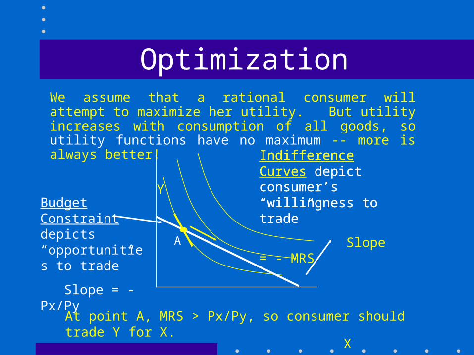
OptimizationWe assume that a rational consumer will attempt to maximize her utility. But utility increases with consumption of all goods, so utility functions have no maximum -- more is always better!
Y Utility = No. of Apples + 2(No. of Oranges)
U
X
Indifference Curves depict consumer’s “willingness to trade”
Budget Constraint depicts “opportunities to trade”
Slope = - Px/Py
Indifference Curves depict consumer’s “willingness to trade”
Slope = - MRS
A
At point A, MRS > Px/Py, so consumer should trade Y for X.
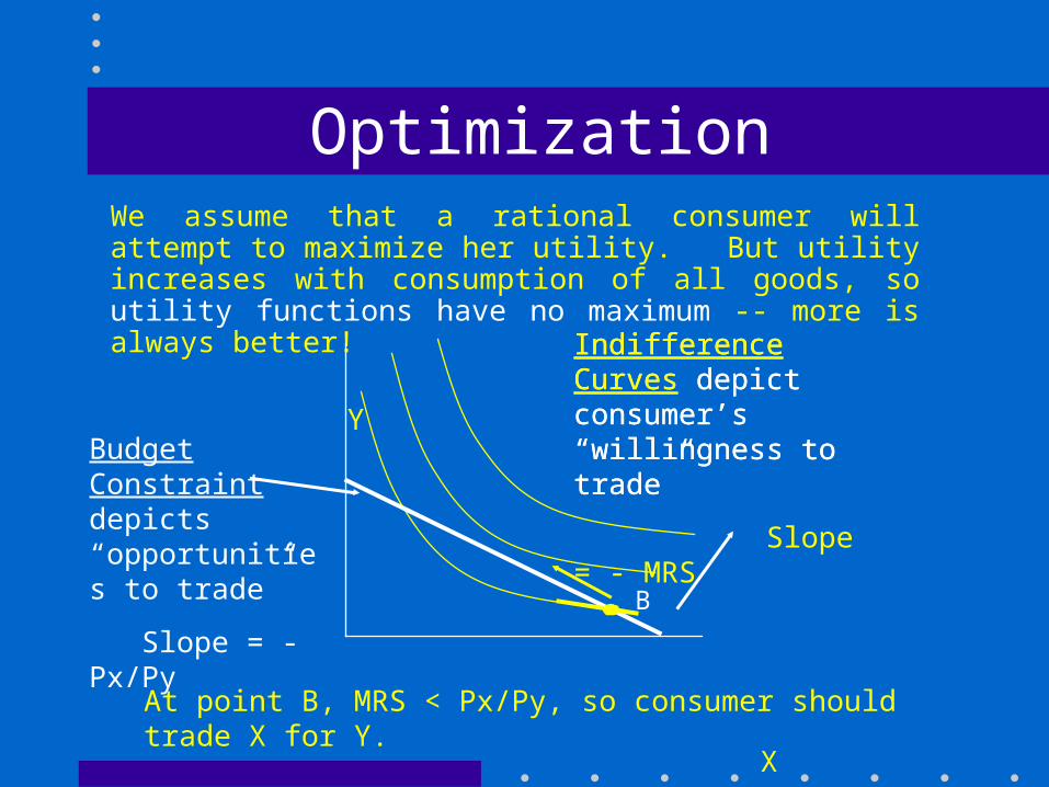
OptimizationWe assume that a rational consumer will attempt to maximize her utility. But utility increases with consumption of all goods, so utility functions have no maximum -- more is always better!
Y Utility = No. of Apples + 2(No. of Oranges)
U
X
Indifference Curves depict consumer’s “willingness to trade”
Budget Constraint depicts “opportunities to trade”
Slope = - Px/Py
Indifference Curves depict consumer’s “willingness to trade”
Slope = - MRS
B
At point B, MRS < Px/Py, so consumer should trade X for Y.

OptimizationThe optimal consumption bundle places the consumer on the highest feasible indifference curve, given her preferences and the opportunities to trade (her income & the prices she faces).
Y Utility = No. of Apples + 2(No. of Oranges)
U
Y*
X* X
Indifference Curves depict consumer’s “willingness to trade”
Slope = - MRSBudget Constraint depicts “opportunities to trade”
Slope = - Px/Py
At point C, MRS = Px/Py, so consumer can’t improve thru trade.
C

Two Conditions for Optimization under Constraint:
1. PxX + PyY = I Spend entire budget
2. MRSyx = Px/Py Tangency
Optimization
MRSyx = MUx/MUy = Px/Py
=> MUx/Px = MUy/Py
The marginal utility of the last dollar spent on each good should be the same.
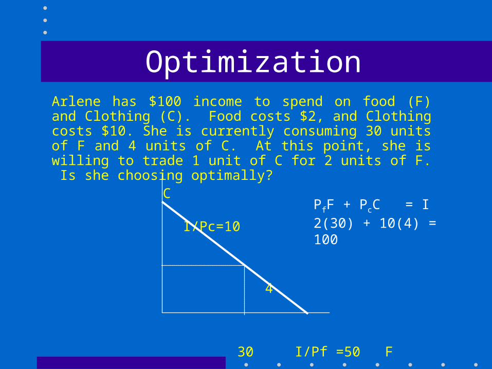
OptimizationArlene has $100 income to spend on food (F) and Clothing (C). Food costs $2, and Clothing costs $10. She is currently consuming 30 units of F and 4 units of C. At this point, she is willing to trade 1 unit of C for 2 units of F. Is she choosing optimally?
C Utility = No. of Apples + 2(No. of Oranges) I/Pc=10 U
4
30 I/Pf =50 F
PfF + PcC = I2(30) + 10(4) = 100
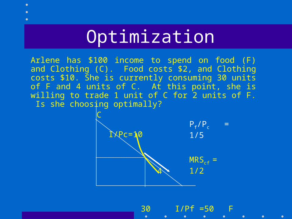
OptimizationArlene has $100 income to spend on food (F) and Clothing (C). Food costs $2, and Clothing costs $10. She is currently consuming 30 units of F and 4 units of C. At this point, she is willing to trade 1 unit of C for 2 units of F. Is she choosing optimally?
C Utility = No. of Apples + 2(No. of Oranges) I/Pc=10 U
4
30 I/Pf =50 F
Pf/Pc = 1/5
MRScf = 1/2
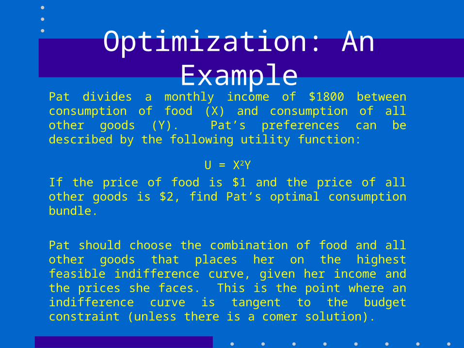
Optimization: An ExamplePat divides a monthly income of $1800 between consumption of food (X) and consumption of all other goods (Y). Pat’s preferences can be described by the following utility function:
U = X2Y
If the price of food is $1 and the price of all other goods is $2, find Pat’s optimal consumption bundle.
Pat should choose the combination of food and all other goods that places her on the highest feasible indifference curve, given her income and the prices she faces. This is the point where an indifference curve is tangent to the budget constraint (unless there is a comer solution).

Optimization: An ExamplePat divides a monthly income of $1800 between consumption of food (X) and consumption of all other goods (Y). Pat’s preferences can be described by the following utility function:
U = X2Y
If the price of food is $1 and the price of all other goods is $2, find Pat’s optimal consumption bundle.
Since Pat’s utility function is U = X2Y, MUx = 2XY and MUy = X2. MRS = (-)MUx/MUy = (-)2XY/X2 = (-)2Y/X. Setting this equal to the (-)price ratio (Px/Py), we find ½ = 2Y/X, X = 4Y. This is Pat’s optimal ratio of the goods, given prices.
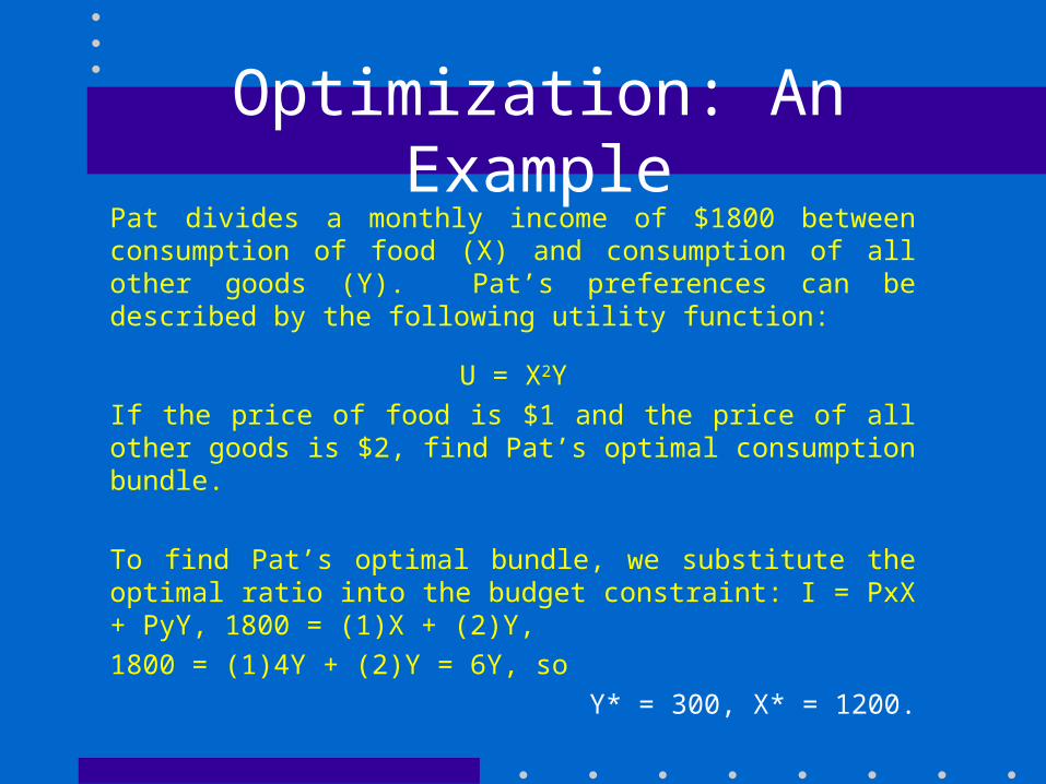
Optimization: An ExamplePat divides a monthly income of $1800 between consumption of food (X) and consumption of all other goods (Y). Pat’s preferences can be described by the following utility function:
U = X2Y
If the price of food is $1 and the price of all other goods is $2, find Pat’s optimal consumption bundle.
To find Pat’s optimal bundle, we substitute the optimal ratio into the budget constraint: I = PxX + PyY, 1800 = (1)X + (2)Y,
1800 = (1)4Y + (2)Y = 6Y, so
Y* = 300, X* = 1200.
Y
X
900
Y*=300
600 X*=1200
U = XY
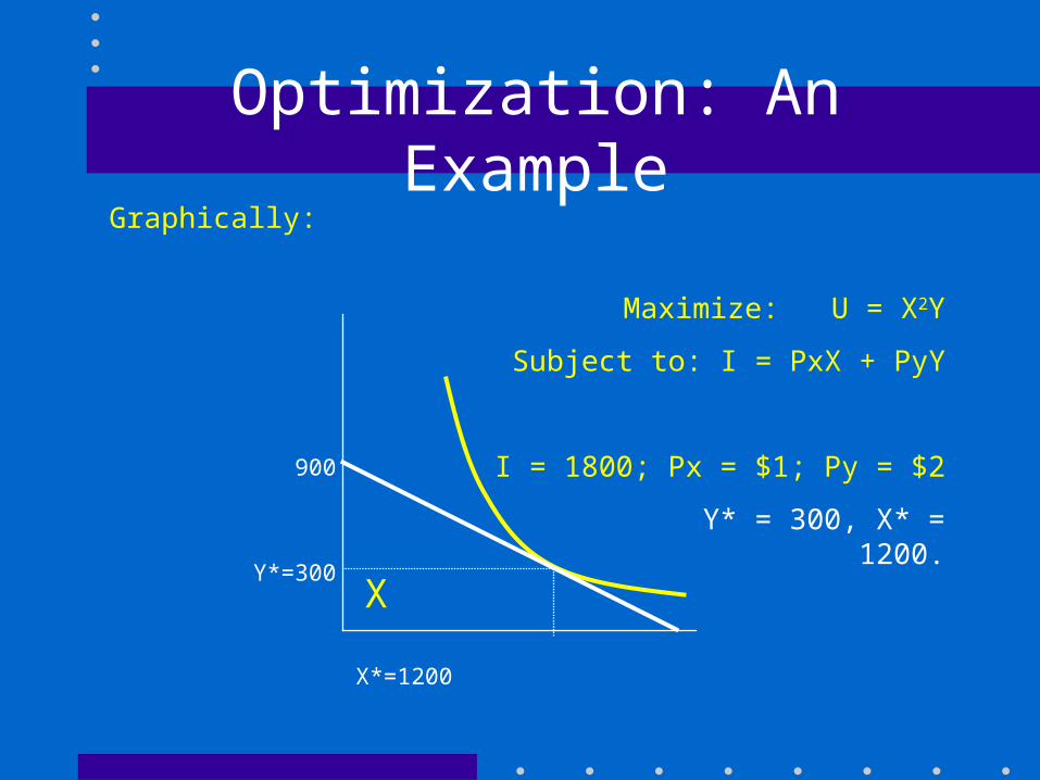
Optimization: An ExampleGraphically:
Maximize: U = X2Y
Subject to: I = PxX + PyY
I = 1800; Px = $1; Py = $2
Y* = 300, X* = 1200.
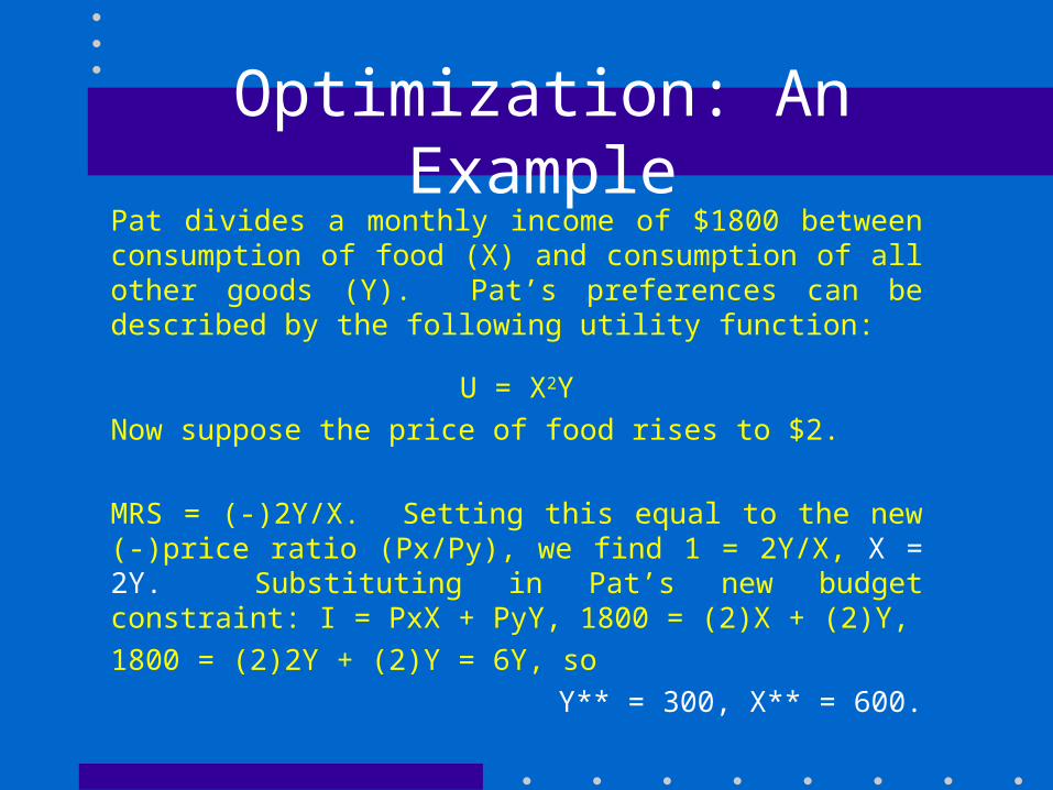
Optimization: An ExamplePat divides a monthly income of $1800 between consumption of food (X) and consumption of all other goods (Y). Pat’s preferences can be described by the following utility function:
U = X2Y
Now suppose the price of food rises to $2.
MRS = (-)2Y/X. Setting this equal to the new (-)price ratio (Px/Py), we find 1 = 2Y/X, X = 2Y. Substituting in Pat’s new budget constraint: I = PxX + PyY, 1800 = (2)X + (2)Y,
1800 = (2)2Y + (2)Y = 6Y, so
Y** = 300, X** = 600.
Y
X
900
Y*=300
600 X*=1200
U = XY
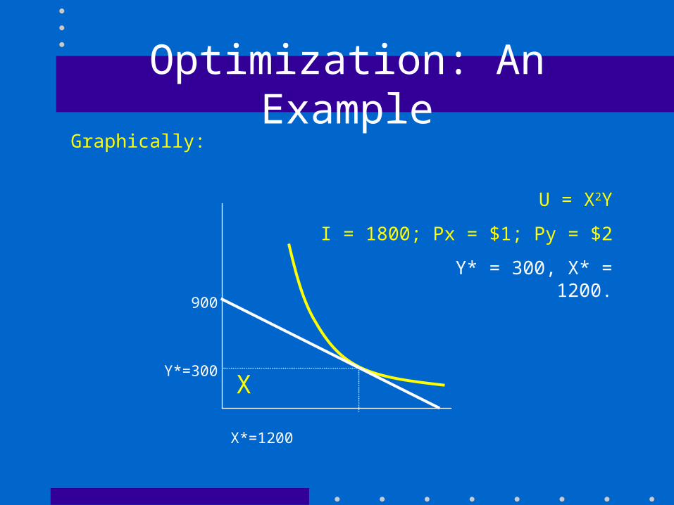
Optimization: An ExampleGraphically:
U = X2Y
I = 1800; Px = $1; Py = $2
Y* = 300, X* = 1200.

Y
X
900
Y**=300
X**= 600 12001200
U = XY
Optimization: An ExampleGraphically:
Now: U = X2Y
I = 1800; Px’ = $2; Py = $2
Y* = 300, X* = 600.
Y
X
900
Y**=300
X**= 600 1200 1200
U = XY
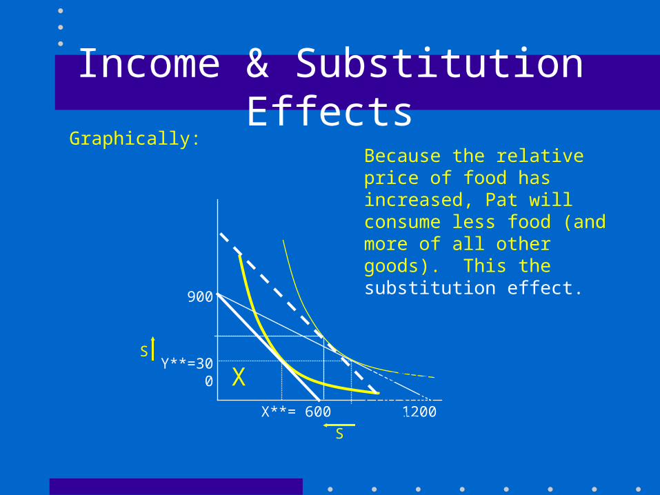
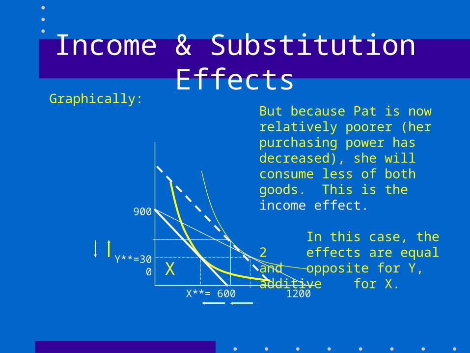
Graphically:Because the relative price of food has increased, Pat will consume less food (and more of all other goods). This the substitution effect. But because Pat is now relatively poorer (her purchasing power has decreased), she will consume less of both goods. This is the income effect.
Income & Substitution Effects
S
S
Y
X
900
Y**=300
X**= 600 1200 1200
U = XY
Graphically:But because Pat is now relatively poorer (her purchasing power has decreased), she will consume less of both goods. This is the income effect.
In this case, the 2 effects are equal and opposite for Y, additive for X.
Income & Substitution Effects
Next Time
How to consumers respond to changes in income and prices?

Next Time
7/2 Individual and Market Demand
Pindyck & Rubenfeld, Chapters 2 (review) & 4
Besanko, Chapters 2 (review) & 5