unit root tests - 國立中興大學web.nchu.edu.tw/~finmyc/tim_unit_p.pdfroots on the unit circle,...

$: Unit Root Tests - 國立中興大學web.nchu.edu.tw/~finmyc/tim_unit_p.pdfroots on the unit circle, {yt} is said to be an I(d) process (integratedprocess of order d). That is, an I(d)$
Unit Root Tests

Mei-Yuan Chen

Department of Finance

National Chung Hsing University

February 25, 2013

M.-Y. Chen I(0) vs I(1)

Unit Root Tests

An ARMA(p,q) (autoregressive of order p and moving average

of order q) model of yt is typically written as

Φ(B)yt = Ψ(B)ǫt, where

Φ(B) = 1− φ1B − φ2B2 − · · · − φpB

p,

Ψ(B) = 1− ψ1B − ψ2B2 − · · · − ψqB

q,

are polynomials in B, the back-shift operator, and {ǫt} is

white-noise.


Stationarity

An ARMA model is said to be “stationary” if all the roots of

Φ(z) = 0 are outside the unit circle, |z| = 1. In this case, we

can obtain a stationary solution yt = Φ(B)−1Ψ(B)ǫt.


Invertibility

An ARMA model is said to be “invertible” if all the roots of

Ψ(z) = 0 are outside the unit circle. In this case, we can write

ǫt = Ψ(B)−1Φ(B)yt. For example, if yt = αyt−1 + ǫt, then

{yt} is stationary provided that the root of Φ(z) = 1−αz = 0,

z = 1/α, is outside the unit circle, i.e., |α| < 1.


ARIMA Models

An ARIMA(p,d,q) model of yt is Φ(B)(l − B)dyt = Ψ(B)ǫt,

where Φ(B) and Ψ(B) satisfy the stationarity and invertibility

conditions. As the polynomial A(z) ≡ Φ(z)(1 − z)d = 0 has d

roots on the unit circle, {yt} is said to be an I(d) process

(integrated process of order d). That is, an I(d) process must

be differenced d times to achieve stationarity; in particular, an

I(0) process is stationary.


Of particular interest to us are I(1) processes of the following

form: (1−B)yt = ut, where ut has a stationary and invertible

ARMA representation. To see the properties of an I(1)

process, consider a special case where {yt} is a “random

walk”, i.e., the innovations ut are i.i.d. with mean zero and

finite variance σ2u. That is,

yt = yt−1 + ut, ut ∼ i.i.d.(0, σ2u).


Properties of a Random Walk

1. the effects of past ut on yt are permanent;

2. yt has unbounded variance tσ2u;

3. yt has a smooth sample path (in terms of level crossing)

which typically wanders away and rarely crosses its mean

level. By contrast, an I(0) process has short memory,

bounded variance, and a ragged sample path which

crosses its mean level very often.


Clearly, an I(1) process is non-stationary, but a non-stationary

series need not be I(1). If (1− B)yt has a non-zero mean µ0

such that (1−B)yt = µ0 + ut, then {yt} is said to be an I(1)

process with the drift µ0(since yt = µ0t +∑t

i=0 ut−i. A major

problem in time-series regressions of an I(1) variable is that

many known results are no longer valid.


I(1) without Drift

Consider the DGP (data generating process):

yt = α0yt−1 + ut,

where ut is an I(0) process. We want to test the null

hypothesis of a unit root (α0 = 1) against the alternative

hypothesis that yt is I(0) (|α0| < 1).


Dickey-Fuller Tests

Suppose that we estimate one of the following three models.

yt = α1Tyt−1 + ut, (1)

yt = µ2T + α2Tyt−1 + ut, (2)

yt = µ3T + β3T

(

t− T

2

)

+ α3Tyt−1 + ut, (3)

where ut is a generic notation for OLS residual.


If ut is i.i.d. N(0, σ2u), Dickey & Fuller (1979) show that under

the null hypothesis T (αiT − 1) and the t-statistics

ταiT= (αiT − 1)/[s.e.(αiT )], i = 1, 2, 3,

τµiT= µiT/[s.e.(µiT )], i = 2, 3,

τβ3T= β3T /[s.e.(β3T )],

have non-normal limiting distributions, where s.e. stands for

the OLS standard errors.


The empirical distributions of T (αiT − 1) and ταiT, i = 1, 2, 3

are tabulated in Fuller (1976, p. 371 & p. 373); the

distributions of the t-ratios τµiT, i = 2, 3 and τβ3T

are

tabulated in Dickey & Fuller (1981). From the table for

T (α1T − 1) it can be seen that this distribution is skewed to

the left and α1T is downward biased.


Table Finite-sample and asymptotic critical values of the

Dickey-Fuller test.

Sample Significance Level

Size 1% 2.5% 5% 10%

25 −3.75 −3.33 −3.00 −2.63

50 −3.58 −3.22 −2.93 −2.60

100 −3.51 −3.17 −2.89 −2.58

250 −3.46 −3.14 −2.88 −2.57

∞ −3.43 −3.12 −2.86 −2.57


The distributions of T (αiT − α0) when α0 = −1 are just the

mirror images of those for α0 = 1, in the sense that

P{αiT − α0 > c|α0 = 1} = P{αiT − α0 < −c|α0 = −1}.

Homework! Simulate and plot the empirical distributions of

αiT under the DGPs (data generating process) with α0 = 1

and α0 = −1 for T = 100 and replications 2000.


Augmented Dickey-Fuller TestsMore generally, suppose that ut has an ARMA(p, q)

representation: Φ(B)ut = Ψ(B)ǫt, where ǫt are i.i.d. N(0, σ2).

First consider the case that p = q = 1. Then

ut − φ1ut−1 = ǫt − ψ1ǫt−1, and

ǫt

= ut − φ1ut−1 + ψ1ǫt−1

= (ut − φ1ut−1) + ψ1(ut−1 − φ1ut−2 + ψ1ǫt−2)

= (ut − φ1ut−1) + ψ1(ut−1 − φ1ut−2) + ψ21(ut−2 − φ1ut−3 + ψ1ǫt−3)

=...

=

∞∑

j=0

ψj1(ut−j − φ1ut−1−j).


We have, since ǫt−1 =∑

∞

j=1 ψj−11 (ut−j − φ1ut−1−j),

yt − yt−1

= (α0yt−1 + ut)− yt−1

= (α0 − 1)yt−1 + φ1ut−1 − ψ1ǫt−1 + ǫt

= (α0 − 1)yt−1 + φ1ut−1 − ψ1

∞∑

j=1

ψj−11 (ut−j − φ1ut−1−j) + ǫt

= (α0 − 1)yt−1 + (φ1 − ψ1)[ut−1 + ψ1ut−2 + ψ21ut−3 + · · · ] + ǫt.


This suggests a regression of ∆yt on yt−1 and ∆yt−1, ∆yt−2,

. . . , which can be approximated using an autoregression of

finite order k:

∆yt ≈ (α0 − 1)yt−1 +

(φ1 − π1)[∆yt−1 + ψ1∆yt−2 + ψ21∆yt−3 + · · ·

+ψk−11 ∆yt−k] + ǫt

=: θ0yt−1 + θ1∆yt−1 + θ2∆yt−2 + · · ·+ θk∆yt−k + ǫt.


To obtain consistent estimates, the order of autoregression, k,

must be a function of T ; in particular, Said & Dickey (1984)

show that k must be o(T 1/3) and that there exist c > 0 and

r > 0 such that ck > T 1/r.


On the other hand, the t-statistic for θ0T has the same limiting

distribution as that of τα1T; hence the table in Fuller (1976)

can be used. If a constant term is included in the model, the

resulting t-statistic has the same limiting distribution as that

of τα2T. The same idea carries over if ut follows an

ARMA(p, q) model. Tests of this type are known as the

Augmented Dickey-Fuller (ADF) tests.


Phillips-Perron Tests

More general results are available when ut are weakly

dependent. Let

σ2 := limT→∞

1

TE

[

(

T∑

t=1

ut

)2]

, σ2u := lim

T→∞

1

T

T∑

t=1

E(ut)2.


Define YT in D[0, 1] as

YT (r) =1

σ√T

[Tr]∑

t=1

ut,

where [Tr] denotes the integer part of Tr. We assume

suitable conditions under which the FCLT holds, i.e.,

YT ⇒W , where W is a standard Wiener process. More

specific conditions can be found in, e.g., Phillips (1987) and

Wooldridge & White (1988).


The results below are fundamental for Phillips (1987) and

many other papers written by Phillips and his co-authors.

Without loss of generality we set y0 = 0. Let

W ∗ = W −∫ 1

0W (r) dr. If yt =

∑ti=1 ui,

(1) T−3/2∑T

t=1 yt−1 ⇒ σ

∫ 1

0

W (r) dr;

(2) T−2∑T

t=1 y2t−1 ⇒ σ2

∫ 1

0

W (r)2 dr;


(3) T−1∑T

t=1 yt−1ut ⇒

σ2

∫ 1

0

W (r) dW (r) +1

2(σ2 − σ2

u) =1

2(σ2W (1)2 − σ2

u);

(4) T−3/2∑T

t=1 tut ⇒

σ

∫ 1

0

r dW (r) = σ

(

W (1)−∫ 1

0

W (r) dr

)

;

(5) T−5/2∑T

t=1 tyt−1 ⇒ σ

∫ 1

0

rW (r) dr;

(6) T−2∑T

t=1(yt−1 − y−1)

2 ⇒ σ2

∫ 1

0

W ∗(r)2 dr;

(7) T−1∑T

t=1(yt−1 − y−1)ut ⇒

σ2

∫ 1

0

W ∗(r) dW (r) +1

2(σ2 − σ2

u) .


Under the null hypothesis that yt = yt−1 = ut, where {ut}satisfies the FCLT, then

(a) For model (1),

T (α1T − 1) ⇒12

(

W (1)2 − σ2u/σ

2)

∫ 1

0W (r)2 dr

;

τα1T⇒

σ2σu

(

W (1)2 − σ2u/σ

2)

(

∫ 1

0W (r)2 dr

)1/2.


(b) Let λ = 12(σ2 − σ2

u) and λ∗ = λ/σ2. For model (2),

T (α2T − 1) ⇒∫ 1

0W ∗(r) dW (r) + λ∗∫ 1

0W ∗(r)2 dr

;

and


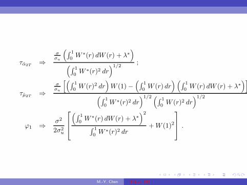
τα2T⇒

σσu

(

∫ 1

0W ∗(r) dW (r) + λ∗

)

(

∫ 1

0W ∗(r)2 dr

)1/2;

τµ2T⇒

σσu

[(

∫ 1

0 W (r)2 dr)

W (1)−(

∫ 1

0 W (r) dr) (

∫ 1

0 W (r) dW (r) + λ∗)]

(

∫ 1

0 W∗(r)2 dr

)1/2 (∫ 1

0 W (r)2 dr)1/2

ϕ1 ⇒ σ2

2σ2u

(

∫ 1

0W ∗(r) dW (r) + λ∗

)2

∫ 1

0W ∗(r)2 dr

+W (1)2

.


Remarks

(1) For model (3), the limits of T (α3T − 1), τµ3T, τβ3T

, and

τα3Tcan be found in Phillips & Perron (1988), and the

limits of φ2 and φ3 can be found in Perron (1990).

(2) The OLS estimators αiT , i = 1, 2, 3, are all ”supper

consistent” in the sense that αiT − 1 is Op(T−1), whereas

in the standard case such that |α0| < 1, αiT − α0 is

Op(T−1/2). Moreover, the OLS estimators remain

consistent even when yt−1 and serially correlated

disturbances are both present because the sample

variation∑T

t=1 y2t−1 grows much faster than the

regressor-error correlation∑T

t=1 yt−1ut.


Note that under the null hypothesis, the estimators σ2T = T−1

∑Tt=1 u

2t

and T−1∑T

t=1(yt − yt−1)2 are consistent for σ2

u by suitable law of large

numbers. Also observe that σ2 is the limit of

1

TE

[

(

T∑

t=1

ut

)2]

=1

T

(

T∑

t=1

E(u2t ) + 2T−1∑

τ=1

T∑

t=τ+1

E(utut−τ )

)

,

which can be consistently estimated using the following (non-parametric)

estimator

s2T,n(T ) =1

T

T∑

t=1

u2t + 2

n(T )∑

τ=1

wτn

T∑

t=τ+1

utut−τ

,

where w(·) is some kernel.


Note that n(T ) characterizes kernel’s bandwidth which should be

growing with T but at a slower rate; especially, n(T ) can be o(T 1/2). If

we use the so-called Bartlett kernel:

wτn =

{

1− τ/(n(T ) + 1), if 0 ≤ τ/n(T ) ≤ 1,

0, otherwise,

we obtain the Newey & West (1987) estimator; if we use the so-called

Parzen kernel:

wτn =

1− 6[τ/n(T )]2 + 6[τ/n(T )]3, if 0 ≤ τ/n(T ) ≤ 1/2,

2[1− τ/n(T )]3, if1/2 ≤ τ/n(T ) ≤ 1,

0, otherwise,

we obtain the Gallant (1987) estimator.


Limiting Distributions of D-F Tests

If ut are i.i.d. with mean zero and variance σ2, then σ2u = σ2

and λ = λ∗ = 0. Under the null hypothesis that

yt = yt−1 + ut, where {ut} satisfies the FCLT, then:

(a) For model (1),

T (α1T − 1) ⇒12

(

W (1)2 − 1)

∫ 1

0W (r)2 dr

;

τα1T⇒

12

(

W (1)2 − 1)

(

∫ 1

0W (r)2 dr

)1/2.


(b) for model (2),

T (α2T − 1) ⇒∫ 1

0W ∗(r) dW (r)∫ 1

0W ∗(r)2 dr

;

τα2T⇒

(

∫ 1

0W ∗(r) dW (r)

)

(

∫ 1

0W ∗(r)2 dr

)1/2;

τµ2T⇒

(

∫ 1

0 W (r)2 dr)

W (1)−(

∫ 1

0 W (r) dr) (

∫ 1

0 W (r) dW (r))

(

∫ 1

0W ∗(r)2 dr

)1/2 (∫ 1

0W (r)2 dr

)1/2

ϕ1 ⇒ 1

2

(

∫ 1

0W ∗(r) dW (r)

)2

∫ 1

0W ∗(r)2 dr

+W (1)2

.


PP Z-Test

As the limits of the DF tests depend on nuisance parameters

when ut are weakly dependent, critical values cannot be

tabulated. Fortunately, the nuisance parameters can be

eliminated even when ut are not i.i.d.


Consider

Z(α1T ) = T (α1T − 1) −12 (s

2Tn − σ2

T )

T−2∑T

t=1 y2t−1

⇒12 (W (1)2 − σ2

u/σ2)

∫ 1

0 W (r)2 dr−

12 (σ

2 − σ2u)

σ2∫ 1

0 W (r)2 dr

=12 (W (1)2 − 1)∫ 1

0W (r)2 dr

,

which is the same as the limit of T (α1T − 1). Therefore, the table in

Fuller (1976) can be directly used for this test. A modified

Z ′α = Z(α1T )/

√2 is related to the empirical tables in Evans &

Savin (1981).


Similarly,

Z(τα1T) =

σTsTn

τα1T−

12 (s

2Tn − σ2

T )

sTn

(

T−2∑T

t=1 y2t−1

)1/2

⇒12 (W (1)2 − σ2

u/σ2)

(

∫ 1

0 W (r)2 dr)1/2

−12 (σ

2 − σ2u)

σ2(

∫ 1

0 W (r)2 dr)1/2

=12 (W (1)2 − 1)

(

∫ 1

0W (r)2 dr

)1/2.


Dickey-Fuller Tests with GLS Detrending Data

ERS (1996) propose a simple modification of the ADF tests inwhich the data are detrended so that explanatory variables are”taken out” of the data prior to running the test regression.ERS define a quasi-difference of that depends on the valuerepresenting the specific point alternative against which wewish to test the null:

d(yt|a) ={

yt if t = 1,

yt − ayt−1 if t < 1,, d(xt|a) =

{

xt if t = 1,

xt − ayt−1 if t < 1,


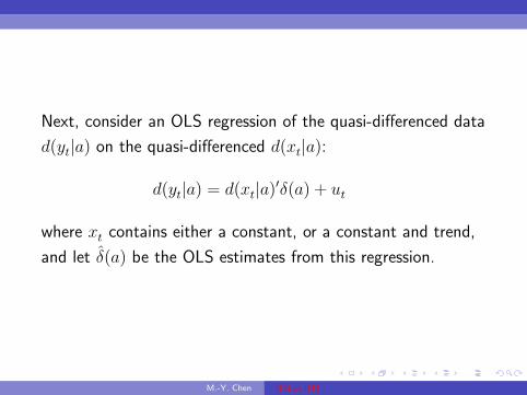
Next, consider an OLS regression of the quasi-differenced data

d(yt|a) on the quasi-differenced d(xt|a):

d(yt|a) = d(xt|a)′δ(a) + ut

where xt contains either a constant, or a constant and trend,

and let δ(a) be the OLS estimates from this regression.


Now, all that we need know is a value for a. ERS recommend

the use of a, where:

a =

{

1− 7T

ifxt = 1,

1− 13.5T

ifxt = (1, t)′.

Then, define the GLS detrended data, ydt using the estimates

associated with the a:

ydt = yt − x′tδ(a).


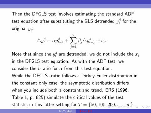
Then the DFGLS test involves estimating the standard ADF

test equation after substituting the GLS detrended ydt for the

original yt:

△ydt = αydt−1 +

p∑

j=1

βj△ydt−j + vt.

Note that since the ydt are detrended, we do not include the xtin the DFGLS test equation. As with the ADF test, we

consider the t-ratio for α from this test equation.

While the DFGLS -ratio follows a Dickey-Fuller distribution in

the constant only case, the asymptotic distribution differs

when you include both a constant and trend. ERS (1996,

Table 1, p. 825) simulate the critical values of the test

statistic in this latter setting for T = {50, 100, 200, . . . ,∞}.M.-Y. Chen I(0) vs I(1)

Homework! Simulate the empirical sizes and powers of ADF

and DFGLS tests under the DGP: yt = 0.1 + α0yt−1 + ut with

α0 = 1 and α0 = 0.8. The sample size and replications are

considered as T = 100 and 2000.


Unit Root Tests in gretl

The unit root tests of ADF and ADF-GLS are provided in

gretl. These two tests are accessed via 「Variable (V)」 in tool

bar of gretl.


Unit Root Tests in R

The following packages in R provide unit root tests:

1. urca; see twi−unit.R

2. tseries

3. fUnitRoots

In urca, the unit root tests can be implemented by using

urTest(x, method = c(”unitroot”, ”adf”, ”urers”, ”urkpss”, ”urpp”,

”ursp”, ”urza”), title = NULL, description = NULL, ...)


Unit Root Tests in urca

1. ur.df: Augmented-Dickey-Fuller Unit Root Test

ur.df(y, type = c(”none”, ”drift”, ”trend”), lags = 1, selectlags =

c(”Fixed”, ”AIC”, ”BIC”))

2. ur.ers: Elliott, Rothenberg & Stock Unit Root Test

ur.ers(y, type = c(”DF-GLS”, ”P-test”), model = c(”constant”,

”trend”), lag.max = 4)

3. ur.kpss: Kwiatkowski et al. Unit Root Test

ur.kpss(y, type = c(”mu”, ”tau”), lags = c(”short”, ”long”, ”nil”),

use.lag = NULL)

4. ur.pp: Phillips & Perron Unit Root Test

ur.pp(x, type = c(”Z-alpha”, ”Z-tau”), model = c(”constant”,

”trend”), lags = c(”short”, ”long”), use.lag = NULL)


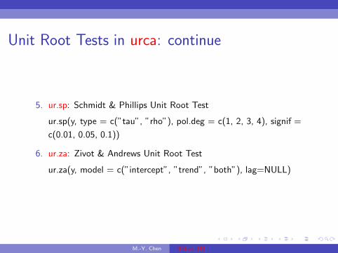
Unit Root Tests in urca: continue

5. ur.sp: Schmidt & Phillips Unit Root Test

ur.sp(y, type = c(”tau”, ”rho”), pol.deg = c(1, 2, 3, 4), signif =

c(0.01, 0.05, 0.1))

6. ur.za: Zivot & Andrews Unit Root Test

ur.za(y, model = c(”intercept”, ”trend”, ”both”), lag=NULL)


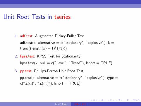
Unit Root Tests in tseries

1. adf.test: Augmented Dickey-Fuller Test

adf.test(x, alternative = c(”stationary”, ”explosive”), k =

trunc((length(x)− 1)(1/3)))

2. kpss.test: KPSS Test for Stationarity

kpss.test(x, null = c(”Level”, ”Trend”), lshort = TRUE)

3. pp.test: Phillips-Perron Unit Root Test

pp.test(x, alternative = c(”stationary”, ”explosive”), type =

c(”Z(α)”, ”Z(tα)”), lshort = TRUE)


Unit Root Tests in fUnitRoots

1. adfTest: Augmented Dickey-Fuller test for unit roots,

adfTest(x, lags = 1, type = c(”nc”, ”c”, ”ct”), title = NULL,

description = NULL)

2. unitrootTest: the same based on McKinnons’s test statistics.

unitrootTest(x, lags = 1, type = c(”nc”, ”c”, ”ct”), title = NULL,

description = NULL)

3. urdfTest: Augmented Dickey-Fuller test for unit roots,

4. urersTest: Elliott-Rothenberg-Stock test for unit roots,

5. urkpssTest: KPSS unit root test for stationarity,

6. urppTest: Phillips-Perron test for unit roots,

7. urspTest: Schmidt-Phillips test for unit roots,

8. urzaTest: Zivot-Andrews test for unit roots.M.-Y. Chen I(0) vs I(1)

Testing Stationarity Against a Unit Root

We have learned that the DF tests usually have low power

against trend stationarity. To complement the aforementioned

unit-root tests, it is quite natural to consider tests from an

opposite direction, i.e., tests of the null hypothesis of (trend)

stationarity against a unit root.


KPSS Tests

Consider a linear regression model

yt = xtat + z′tb0 + ǫt, t = 1, · · · , T,

where at = at−1 + vt with the initial value a0, and vt are i.i.d.

N(0, σ2v) independent of ǫt which are also i.i.d. N(0, σ2

ǫ ).

Under the null that at = a0, σ2v = 0. Under the alternative of

random walk,

yt = xta0 + z′tb0 + xt

t∑

j=1

vj + ǫt, t = 1, · · · , T.


Nabeya & Tanaka (1988) derive the locally best invariant test

for σ2v = 0, which is based on the ratio of two quadratic forms:

e′DxATDxe

e′e,

where Dx = diag(x1, . . . , xT ), AT is such that its (s, t)th

element is min(s, t), and e is the residual vector from

regressing yt on xt and zt.


Kwiatkowski, Phillips, Schmidt, & Shin (1992) apply this test

to test for the null of (trend) stationarity. Consider the DGP:

yt = a0 + b0t+ ǫt,

which is a special case of the null model of Nabeya &

Tanaka (1988) with xt = 1 and zt = t; when b0 = 0, this is

just a level-stationary model. Under the alternative that yt is

an I(1) process with drift,

yt = a0 + b0t + y∗t ,

where y∗t =∑t

j=1 vj .


Note that AT can be written as C ′

TCT , where CT is an upper

triangular matrix with all elements on and above the main

diagonal being 1. In this case, Dx = IT so that

e′DxATDxe = e′C ′

TCT e, and it can be verified that CT e is a

vector containing reversed partial sums of et, i.e., the t-th

element is Rt =∑T

i=t ei. Let St denote partial sums of et.

Then, R1 = ST = 0 and St = −Rt+1 for t = 1, . . . , T − 1.


Nabeya and Tanaka’s statistics can be written as:

ηi =T−2

∑Tt=1R

2t

σ2T

=T−2

∑Tt=1 S

2t

σ2T

, i = 1, 2,

with σ2T = e′e/T , where e is obtained from regressing yt on

the constant 1 for the null of level stationarity (i = 1) and

from regressing yt on 1 and t for the null of trend stationarity

(i = 2).


To allow for weakly dependent and heterogeneous ǫt, the

statistics become

ηi =T−2

∑Tt=1 S

2t

s2Tn

, i = 1, 2,

where s2Tn is the Newey-West or Gallant estimator of

σ2 = limT T−1 IE(S2

T ); these two tests will be referred to as

the KPSS tests.


Theorem: KPSS

In the level-stationary model,

η1 ⇒∫ 1

0

W 0(r)2 dr,

where W 0 is a Brownian bridge; in the trend-stationary model,

η2 ⇒∫ 1

0

V (r)2 dr;

where

V (r) = W (r) + (2r − 3r2)W (1)− (6r − 6r2)∫ 1

0W (s) ds.


These tests suffer similar problems as the PP test. When ǫtare highly correlated, the empirical sizes are too high if the

truncation lag n for s2Tn is too small, say, 4. A large truncation

lag, however, has an adverse effect on the power of test.


Table 2: Asymptotic critical values of the KPSS tests.

Statistic 1% 2.5% 5% 10%

η1 0.739 0.574 0.463 0.347

η2 0.216 0.176 0.146 0.119


Panel Unit Root Tests

Consider the model

yit = ρiyit−1 + z′itγ + uit, i = 1, . . . , N, t = 1, . . . , T, (4)

where zit is the deterministic component and uit is a

stationary process. zit could be zero, one, the fixed effects, µi,

or fixed effects as well as a time trend, t.


Levin and Lin (1992), Levin, Lin, and Chu (2002)Levin and Lin (LL) tests assume that ρi = ρ for all i and are

interesting in testing

H0 : ρ = 1 v.s. Ha : ρ < 1.

Denote ρ as the OLS estimator of ρ in (4), Levin andLin (2002) show that

√NT (ρ− 1) =

1√N

∑Ni=1

1T

∑Tt=1 yi,t−1uit

1N

∑Ni=1

1T 2

∑Tt=1 y

2i,t−1

tρ =(ρ− 1)

√

∑Ni=1

∑Tt=1 y

2i,t−1

se,

s2e =1

TN

N∑

i=1

T∑

t=1

u2it.


As T → ∞ and then N → ∞,zit ρ

0√NT (ρ− 1) ⇒ N(0, 2)

1√NT (ρ− 1) ⇒ N(0, 2)

µi

√NT (ρ− 1) + 3

√N ⇒ N(0, 51/5)

(µi, t)√N(T (ρ− 1) + 7.5) ⇒ N(0, 2895/112)


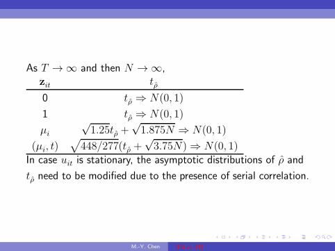
As T → ∞ and then N → ∞,zit tρ

0 tρ ⇒ N(0, 1)

1 tρ ⇒ N(0, 1)

µi

√1.25tρ +

√1.875N ⇒ N(0, 1)

(µi, t)√

448/277(tρ +√3.75N) ⇒ N(0, 1)

In case uit is stationary, the asymptotic distributions of ρ and

tρ need to be modified due to the presence of serial correlation.


Harris and Tzavalis (1999)’s Tests

Harris and Tzavalis (1999) also derived unit root tests for (4)

with zit = {0}, {µi}, or {µi, t} when the time dimension of

the panel, T , is fixed. This is typical case for micro panel

studies. The main results arezit ρ

0√N(ρ− 1) ⇒ N

(

0, 2T (T−1)

)

µi

√N(

ρ− 1 + 3T+1

)

⇒ N(

0, 3(17T2−20T+17)

5(T−1)(T+1)3

)

(µi, t)√N(

ρ− 1 + 152(T+2)

)

⇒ N(

0, 15(193T2−728T+1147)

112(T+1)3(T−2)

)


Im, Pesaran and Shin (2003)’s Tests

The tests of Levin and Lin (1992) are restrictive in the sense

that it requires ρ to be homogeneous across i. Im, Pesaran

and Shin (2003) allow for heterosgeneous coefficient of yit−1

and proposed an alternative testing procedure based on the

augmented DF tests when uit is serially correlated with

different serial correlation properties across cross-sectional

units, i.e., uit =∑pi

j=1 ψijuit−j + ǫit. Substituting this uit in

(4), we get

yit = ρiyit−1 +

pi∑

j=1

ψij△yit−j + z′itγ + ǫit, i = 1, . . . , N, t = 1, . . . , T,


The null hypothesis is

H0 : ρi = 1

for all i against the alternative hypothesis

Ha : ρi < 1

for at least one i. The t-statistic suggested by Im, Pesaran and

Shin (2003) is defined as

t =1

N

N∑

i=1

tρi, (6)

where tρiis the individual t-statistic of testing H0 : ρi = 1 in (5). It is

known that for a fixed N ,

tρi⇒∫ 1

0 WiZdWiZ[

∫ 1

0 W2iZ

]1/2= tiT (7)

as T → ∞.M.-Y. Chen I(0) vs I(1)

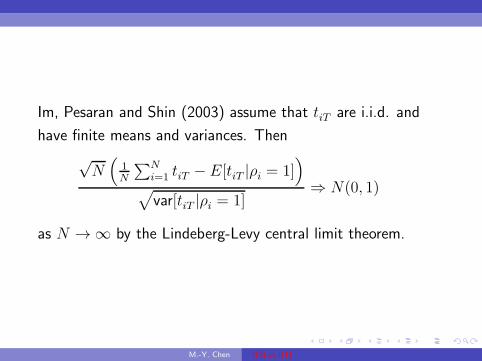
Im, Pesaran and Shin (2003) assume that tiT are i.i.d. and

have finite means and variances. Then

√N(

1N

∑Ni=1 tiT − E[tiT |ρi = 1]

)

√

var[tiT |ρi = 1]⇒ N(0, 1)

as N → ∞ by the Lindeberg-Levy central limit theorem.


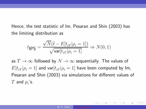
Hence, the test statistic of Im, Pesaran and Shin (2003) has

the limiting distribution as

tIPS =

√N(t− E[tiT |ρi = 1])√

var[tiT |ρi = 1]⇒ N(0, 1)

as T → ∞ followed by N → ∞ sequentially. The values of

E[tiT |ρi = 1] and var[tiT |ρi = 1] have been computed by Im,

Pesaran and Shin (2003) via simulations for different values of

T and pi’s.


Combining p-value TestsLet pi be the p-value of a unit root test for cross-section i, Maddala and

Wu (1999) and Choi (1999) proposed a Fisher type test as:

P = −2

N∑

i=1

ln pi (8)

which combines the p-value from unit root tests for each cross-section i

to test for unit root in panel data. P is distributed as χ2 with 2N

degrees of freedom as Ti → ∞ for all N . When pi closes to 0 (null

hypothesis is rejected), ln pi closes to −∞ so that large value P will be

found and then the null hypothesis of existing panel unit root will be

rejected. In contrast, when pi closes to 1 (null hypothesis is not

rejected), ln pi closes to 0 so that small value P will be found and then

the null hypothesis of existing panel unit root will not rejected.


Choi (1999) pointed out the advantages of the Fisher test: (1) the

cross-sectional dimension, N , can be either finite or infinite, (2) each

group can have different types of nonstochastic and stochastic

components, (3) the time series dimension, T can be different for each i

(imbalance panel data), and (4) the alternative hypothesis would allow

some groups to have unit roots while others may not. A main

disadvantage involved is that the p-value have to be derived by Monte

Carlo simulations.

When N is large, Choi (1999) also proposed a Z test,

Z =

1√N

∑Ni=1(−2 ln pi − 2)

2(9)

since E[−2 ln pi] = 2 and var[−2 ln pi] = 4. Assume pi’s are i.i.d. and

use the Lindeberg-Levy central limit theorem to get

Z ⇒ N(0, 1)

as Ti → ∞ followed by N → ∞.


Hadri (1999)’s Test: KPSS TypeLet eit be the residuals from the regression:

yit = z′

itγ + eit (10)

and σ2e be the estimate of the error variance. Also, let Sit be

the partial sum process of the residuals,

Sit =

t∑

j=1

eij .

Then the LM statistic is

LM =1N

∑Ni=1

1T 2

∑Tt=1 S

2it

σ2e

.


It can be shown that

LM →p E

[∫

WiZ

]

as T → ∞ followed by N → ∞ provided E[∫

W 2iZ] <∞.

Also,

√N(LM − E[

∫

W 2iZ])

√

var[∫

W 2iZ]

⇒ N(0, 1)

as T → ∞ followed by N → ∞.


Panel Unit Roots Tests in R: CADFtest

The asymptotic p-values of the Hansen’s (1995)Covariate-Augmented Dickey Fuller (CADF) test for a unitroot are computed using the approach outlined in Costantiniet al. (2007).

1. CADFpvalues: p-values of the CADF test for unit roots

CADFpvalues(t0, rho2 = 0.5, type=c(”trend”, ”drift”, ”none”))

2. CADFtest: Hansen’s Covariate-Augmented Dickey Fuller (CADF)

test for unit roots


Panel Unit Roots Tests in R: plm

1. purtest: Unit root tests for panel data

purtest(object, data = NULL, index = NULL, test=

c(”levinlin”, ”ips”, ”madwu”, ”hadri”), exo = c(”none”,

”intercept”, ”trend”), lags = c(”SIC”, ”AIC”, ”Hall”),

pmax = 10, Hcons = TRUE, q = NULL, dfcor = FALSE,

fixedT = TRUE, ...)


unit root tests - 國立中興大學web.nchu.edu.tw/~finmyc/tim_unit_p.pdfroots on the unit circle,...

Documents