151

UNIT-V

MTI & PULSE DOPPLER RADAR

Introduction The doppler frequency shift produced by a moving target may be used in a pulse radar just as in the CW radar,

to determine the relative velocity of a target or to separate desired moving targets from undesired stationary objects (clutter).

Although there are applications of pulse radar where a determination of the target's relative Velocity is made from the doppler frequency shift, the use of doppler to separate small moving Targets in the presence of large clutter has probably been of far greater interest. Such a pulse Radar that utilizes the doppler frequency shift as a means for discriminating moving from fixed targets is called an MTI (moving target indication) or a pulse doppler radar. The two are based on the same physical principle, but in practice there are generally recognizable differences between them.

The MTI radar, for instance, usually operates with ambiguous Doppler measurement (so-called blind speeds) but with unambiguous range measurement (no second-time'-around echoes).

The opposite is generally the case for a pulse doppler radar. Its pulse repetition frequency is usually high enough to operate with unambiguous doppler (no blind speeds) but at the expense of range ambiguities.

5.1 Description of operation. A CW radar may be converted into a pulse radar as shown in by providing a power amplifier and a modulator to turn the amplifier on and off for the purpose of generating pulses. The main difference between the pulse radar of Fig. 4.l and the one described in Chap. 1 is that a small portion of the CW oscillator power that generates the transmitted pulses is diverted to the receiver to take the place of the local oscillator. However, this CW signal does more than function as a replacement for the local oscillator. It acts as the coherent reference needed to detect the doppler frequency shift. By coherent it is meant that the phase of the transmitted signal is preserved in the reference signal. The reference signal is the distinguishing feature of coherent MTI radar. If the CW oscillator voltage is represented as A1 sin 2πf0t, Where A1 is the amplitude and f0

is the carrier frequency. Let the reference signal be written as A2 sin 2πf0t The echo signal from a moving target can be written

Vecho = A3 sin { 2π(fo±fd)t - 𝟒𝝅𝒇𝒐𝑹𝒐

𝒄 } = A3 sin { 2π(fo±fd)t - Φo }

Where

152

A2 is the amplitude of reference signal

A3 is the amplitude of echo signal

fd is the Doppler shift in frequency.

Fig 4.1: Simple Pulse Doppler radar

The reference signal and the target echo signal are heterodyned in the mixer stage of the receiver. Only the low-frequency (difference-frequency) component from the mixer is of interest and is a voltage given by

Vdiff = A4 sin { 2πfdt - 𝟒𝝅𝒇𝒐𝑹𝒐

𝒄 }

Note that for stationary targets the doppler frequency shift will be zero; hence Vdiff will not vary with time and may take on any constant value from +A4 to - A4 including zero. However, when the target is in motion relative to the radar, fd has a value other than zero and the Vdiff will be a function of time.

Moving targets may be distinguished from stationary targets by observing the video output on an A-scope (amplitude vs. range). A single sweep on an A-scope might appear as in Fig. 4.2. This sweep shows several fixed targets and two moving targets indicated by the two arrows. On the basis of a single sweep, moving targets cannot be distinguished from fixed targets. Successive A-scope sweeps (pulse-repetition intervals) are shown in Fig. 4.2 a to e. Echoes from fixed targets remain constant throughout, but echoes from moving targets vary in amplitude from sweep to sweep at a rate corresponding to the doppler frequency. The superposition of the successive A-scope sweeps is shown in Fig. 4.2 f The moving targets produce, with time, a "butterfly" effect on the A-scope. Although the butterfly effect is suitable for recognizing moving targets on an A-scope, it is not appropriate for display on the PPI. One method commonly employed to extract Doppler information in a form suitable for display on the PPI scope is with a delay-line canceller (Fig. 4.3).

153

Figure 4.2 (a-e) Successive sweeps of an MTI radar A-scope display (echo

amplitude as a function of time); (f) superposition of many sweeps; arrows indicate position of moving targets.

The delay-line canceller acts as a filter to eliminate the dc component of fixed targets and to pass the ac components of moving targets. The video portion of the receiver is divided into two channels. One is a normal video channel. In the other, the video signal experiences a time delay equal to one pulse-repetition period (equal to the reciprocal of the pulse-

154

repetition frequency). The outputs from the two channels are subtracted from one another. The fixed targets with unchanging amplitudes from pulse to pulse are canceled on subtraction. However, the amplitudes of the moving-target echoes are not constant from pulse to pulse subtraction results in an uncancelled residue.

Figure 4.3: MTI receiver with delay-line canceller.

The output of the subtraction circuit is bipolar video, just as was the input. Before bipolar video can intensity-modulate a PPI display, it must be converted to unipotential voltages (unipolar video) by a full-wave rectifier. 5.1.1 MTI Radar with Power Amplifier Transmitter The simple MT1 radar shown in Fig. 4.l is not necessarily the most typical. The block diagram of a more common MTI radar employing a power amplifier is shown in Fig. 4.4.

Fig 4.4: MTI radar employing a power amplifier

155

The significant difference between this MTI configuration and that of Fig. 4.1 is the manner in which the reference signal is generated. In Fig. 4.4, the coherent reference is supplied by an oscillator called the coho, which stands for coherent oscillator. The coho is a stable oscillator whose frequency is the same as the intermediate frequency used in the receiver. In addition to providing the reference signal, the output of the coho fc is also mixed with the local-oscillator frequency fl . The local oscillator must also be a stable oscillator and is called stalo, for stable local oscillator. The RF echo signal is heterodyned with the stalo signal to produce the IF signal just as in the conventional super-heterodyne receiver. The stalo, coho and the mixer in which they are combined plus any low-level amplification are called the receiver-exciter because of the dual role they serve in both the receiver and the transmitter. The characteristic feature of coherent MTI radar is that tile transmitted signal must be coherent (in phase) with the reference signal in the receiver. This is accomplished in the radar system diagramed in Fig. 4.4 by generating the transmitted signal from the coho reference signal. The function of the stalo is to provide the necessary frequency translation from the IF to the transmitted (RF) frequency. Although the phase of the stalo influences the phase of the transmitted signal, any stalo phase shift is canceled on reception because the stalo that generates the transmitted signal also acts as the local oscillator in the receiver. The reference signal from the coho and the IF echo signal are both fed into a mixer called the phase detector. The phase detector differs from the normal amplitude detector since its output is proportional to the phase difference between the two input signals.

Any one of a number of transmitting-tube types might be used as the power amplifier.

These include the triode, tetrode, klystron amplifier, traveling-wave tube, and the crossed-

field amplifier.

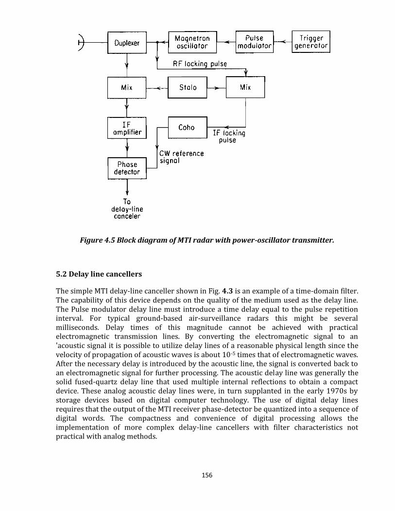
5.1.2. MTI Radar with Power Oscillator Transmitter The block diagram of a typical MTI Radar with Power Oscillator Transmitter is shown in the figure 4.5. Magnetron is normally used as power oscillator. The difference primarily lies in the manner in which the reference signal is generated. Before the development of the klystron amplifier, the only high-power transmitter available at microwave frequencies for radar application was the magnetron oscillator. In an oscillator the phase of the RF bears no relationship from pulse to pulse. For this reason the reference signal cannot be generated by a continuously running oscillator. However, a coherent reference signal may be readily obtained with the power oscillator by readjusting the phase of the coho at the beginning of each sweep according to the phase of the transmitted pulse. The phase of the coho is locked to the phase of the transmitted pulse each time a pulse is generated.

156

Figure 4.5 Block diagram of MTI radar with power-oscillator transmitter.

5.2 Delay line cancellers

The simple MTI delay-line canceller shown in Fig. 4.3 is an example of a time-domain filter. The capability of this device depends on the quality of the medium used as the delay line. The Pulse modulator delay line must introduce a time delay equal to the pulse repetition interval. For typical ground-based air-surveillance radars this might be several milliseconds. Delay times of this magnitude cannot be achieved with practical electromagnetic transmission lines. By converting the electromagnetic signal to an 'acoustic signal it is possible to utilize delay lines of a reasonable physical length since the velocity of propagation of acoustic waves is about 10-5 times that of electromagnetic waves. After the necessary delay is introduced by the acoustic line, the signal is converted back to an electromagnetic signal for further processing. The acoustic delay line was generally the solid fused-quartz delay line that used multiple internal reflections to obtain a compact device. These analog acoustic delay lines were, in turn supplanted in the early 1970s by storage devices based on digital computer technology. The use of digital delay lines requires that the output of the MTI receiver phase-detector be quantized into a sequence of digital words. The compactness and convenience of digital processing allows the implementation of more complex delay-line cancellers with filter characteristics not practical with analog methods.

157

5.2.1.Filter characteristics of the delay-line canceller. The delay-line canceller acts as a filter which rejects the d-c component of clutter. Because of its periodic nature, the filter also rejects energy in the vicinity of the pulse repetition frequency and its harmonics.

The video signal received from a particular target at a range Ro is

V1 = k sin { 2πfdt - Φo }

where Φo = phase shift and k = amplitude of video signal. The signal from the previous transmission, which is delayed by a time T = pulse repetition interval (PRT) is

V2 = k sin { 2πfd (t-T) - Φo }

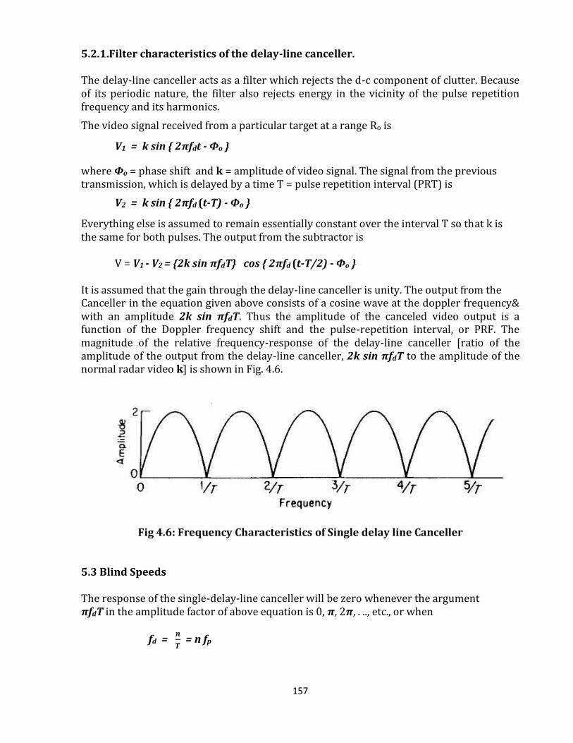
Everything else is assumed to remain essentially constant over the interval T so that k is the same for both pulses. The output from the subtractor is V = V1 - V2 = {2k sin πfdT} cos { 2πfd (t-T/2) - Φo } It is assumed that the gain through the delay-line canceller is unity. The output from the Canceller in the equation given above consists of a cosine wave at the doppler frequency& with an amplitude 2k sin πfdT. Thus the amplitude of the canceled video output is a function of the Doppler frequency shift and the pulse-repetition interval, or PRF. The magnitude of the relative frequency-response of the delay-line canceller [ratio of the amplitude of the output from the delay-line canceller, 2k sin πfdT to the amplitude of the normal radar video k] is shown in Fig. 4.6.

Fig 4.6: Frequency Characteristics of Single delay line Canceller 5.3 Blind Speeds The response of the single-delay-line canceller will be zero whenever the argument πfdT in the amplitude factor of above equation is 0, π, 2π, . .., etc., or when

fd = 𝒏

𝑻 = n fp

158

where n = 0, 1, 2, . . . , and fp = pulse repetition frequency. The delay-line canceller not only eliminates the d-c component caused by clutter (n = 0), but unfortunately it also rejects any moving target whose Doppler frequency happens to be the same as the prf or a multiple thereof. Those relative target velocities which result in zero MTI response are called blind speeds vn and are given by

vn = 𝒏𝝀

𝟐𝑻 =

𝒏𝝀𝒇𝒑

𝟐 n = 0, 1, 2, . . .

The blind speeds are one of the limitations of pulse MTI radar which do not occur with CW radar. They are present in pulse radar because doppler is measured by discrete samples - (pulses) at the prf rather than continuously. If the first blind speed is to be greater than the maximum radial velocity expected from the target, the product 𝝀𝒇𝒑 must be large. Thus the MTI radar must operate at long wavelengths (low frequencies) or with high pulse repetition frequencies, or both. Unfortunately, there are usually constraints other than blind speeds which determine the wavelength and the pulse repetition frequency. Therefore blind speeds might not be easy to avoid. Low radar frequencies have the disadvantage that antenna beamwidths, for a given-size antenna, are wider than at the higher frequencies and would not be satisfactory in applications where angular accuracy or angular resolution is important. The pulse repetition frequency cannot always be varied over wide limits since it is primarily determined by the unambiguous range requirement. Since commercial jet aircraft have speeds of the order of 600 knots, and military aircraft even higher, blind speeds in the MTI radar can be a serious limitation. 5.3.1. Remedy for blind speeds The effect of blind speeds can be significantly reduced, without incurring range ambiguities, by

(a) Operating with more than one pulse repetition frequency. This is called a staggered-PRF MTI.

(b) Operating at more than one RF frequency can also reduce the effect of blind speeds.

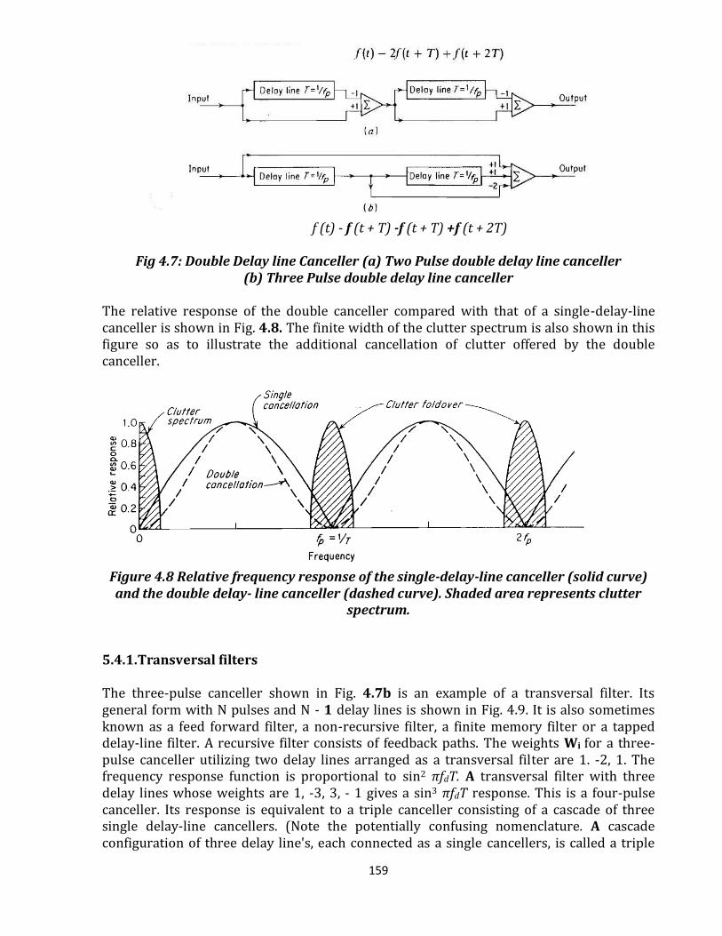
5.4. Enhancement of clutter rejection ratio Double cancellation. The frequency response of a single-delay-line canceller (Fig. 4.3) does not always have as broad a clutter-rejection null as might be desired in the vicinity of d-c. The clutter-rejection notches may be widened by passing the output of the delay-line canceller through a second delay-line canceller as shown in Fig. 4.7. The output of the two single delay-line cancellers in cascade is the square of that from a single canceller. Thus the frequency response is 4 sin2 πfdT. The configuration of Fig. 4.7 is called a double delay-line canceller, or simply a double canceller.

159

f (t) - f (t + T) -f (t + T) +f (t + 2T)

Fig 4.7: Double Delay line Canceller (a) Two Pulse double delay line canceller

(b) Three Pulse double delay line canceller

The relative response of the double canceller compared with that of a single-delay-line canceller is shown in Fig. 4.8. The finite width of the clutter spectrum is also shown in this figure so as to illustrate the additional cancellation of clutter offered by the double canceller.

Figure 4.8 Relative frequency response of the single-delay-line canceller (solid curve) and the double delay- line canceller (dashed curve). Shaded area represents clutter

spectrum.

5.4.1.Transversal filters The three-pulse canceller shown in Fig. 4.7b is an example of a transversal filter. Its general form with N pulses and N - 1 delay lines is shown in Fig. 4.9. It is also sometimes known as a feed forward filter, a non-recursive filter, a finite memory filter or a tapped delay-line filter. A recursive filter consists of feedback paths. The weights Wi for a three-pulse canceller utilizing two delay lines arranged as a transversal filter are 1. -2, 1. The frequency response function is proportional to sin2 πfdT. A transversal filter with three delay lines whose weights are 1, -3, 3, - 1 gives a sin3 πfdT response. This is a four-pulse canceller. Its response is equivalent to a triple canceller consisting of a cascade of three single delay-line cancellers. (Note the potentially confusing nomenclature. A cascade configuration of three delay line's, each connected as a single cancellers, is called a triple

160

cancellers, but when connected as a transversal filter it is called a four-pulse canceller.) The weights for a transversal filter with n delay lines that gives a response sinn πfdT, are the coefficients of the expansion of (1 - x)n which are the binomial coefficients with alternating signs:

Fig 4.9: General form of a transversal (or non-recursive) filter for MTI signal

processing. The transversal filter with alternating binomial weights is closely related to the filter which maximizes the average of the ratio Ic = (S/C)out/(S/C)in where (S/C)out is the signal-to clutter ratio at the output of the filter, and (S/C)in is the signal-to-clutter ratio at the input. The average is taken over the range of doppler frequencies. It is independent of the target velocity and depends only on the weights Wi the autocorrelation function (or power spectrum) describing the clutter, arid the number of pulses. For the two-pulse canceller (a single delay line). the optimum weights based on the above criterion are the same as the binomial weights, when the clutter spectrum is represented by a gaussian function. The difference between a traversal filter with optimal weights and one with binomial weights for a three pulse canceller (two delay lines) is less than 2 dB.4.5 The difference is also small for higher order cancellers.

5.5. Multiple or Staggered PRFs

The use of more than one pulse repetition frequency offers additional flexibility in the design of MTI doppler filters. It not only reduces the effect of the blind speeds, but it also allows a sharper low-frequency cutoff in the frequency response than might be obtained with a cascade of single-delay-line cancellers with sinn πfdT response.

161

The blind speeds of two independent radars operating at the same frequency will be different if their pulse repetition frequencies are different. Therefore, if one radar were " blind " to moving targets, it would be unlikely that the other radar would be " blind" also. Instead of using two separate radars, the same result can be obtained with one radar which time-shares its pulse repetition frequency between two or more different values (multiple prf's). The pulse repetition frequency might be switched every other scan or every time the antenna is scanned a half beamwidth, or the period might be alternated on every other pulse. When the switching is pulse to pulse, it is known as a staggered prf. An example of the composite (average) response response of an MTI radar operating with two separate pulse repetition frequencies on a time-shared basis is shown in Fig. 4.10. The pulse repetition frequencies are in the ratio of 5 : 4. Note that the first blind speed of the composite response is increased several times over what it would be for a radar operating on only a single pulse repetition frequency. Zero response occurs only when the blind speeds of each prf coincide. In the example of Fig. 4.16, the blind speeds are coincident for 4/T1 = 5I T2. Although the first blind speed may be extended by using more than one prf, regions of low sensitivity might appear within the composite passband. The closer the ratio T1 : T2 approaches unity, the greater will be the value of the first blind speed. However, the first null in the vicinity of fd = 1/T1 becomes deeper. Thus the choice of T1/ T2 is a compromise between the value of the first blind speed and the depth of the nulls within the filter pass band. The depth of the nulls can be reduced and the first blind speed increased by operating with more than two PRFs. Figure 4.11 shows the response of a five-pulse stagger (four periods) that might be used with a long-range air traffic control radar.' In this example the periods are in the ratio 25 : 30 : 27 : 31 and the first blind speed is 28.25 times that of a constant prf waveform with the same average period. If the periods of the staggered waveforms have the relationship n1 / T1 = n2 / T2 = . = nN / TN, where n1, n2, ..., N are integers, and if VB is equal to the first blind speed of a non-staggered waveform with a constant period equal to the average period Tav = (T1 + T2 + . . . TN)/N, then the first blind speed is given by

𝑣1

𝑣𝐵 =

𝑛1+𝑛2+⋯…𝑛𝑁

𝑁

162

Figure 4.10 (a) Frequency-response of a single-delay-line canceller for fp = 1/T1;

(b) same for fp = 1/T2; (c) composite response with T1/T2 = 4/5.

Figure 4.11 Frequency response of a five-pulse (four-period) stagger.

A disadvantage of the staggered PRF is its inability to cancel second-time-around clutter echoes. Such clutter does not appear at the same range from pulse to pulse and thus

163

produces un-canceled residue. Second-time-around clutter echoes can be removed by use of a constant PRF. providing there is pulse-to-pulse coherence as in the power amplifier form of MTI. The constant PRF might be employed only over those angular sectors where second-time-around clutter is expected or by changing the PRF each time the antenna scans half-a-beamwidth or by changing the PRF every scan period (rotation of the antenna). 5.6. Range gated doppler filters The delay-line canceller, which can be considered as a time-domain filter, has been widely used in MTI radar as the means for separating moving targets from stationary clutter. It is also possible to employ the more usual frequency-domain bandpass filters of conventional design in MTI radar to sort the doppler-frequency-shifted targets. The filter configuration must be more complex, however, than the single, narrow-bandpass filter. 5.6.1.Collapsing loss A narrowband filter with a passband designed to pass the doppler frequency components of moving targets will "ring" when excited by the usual short radar pulse. That is, its passband is much narrower than the reciprocal of the input pulse width so that the output will be of much greater duration than the input. The narrowband filter "smears" the input pulse since the impulse response is approximately the reciprocal of the filter bandwidth. This smearing destroys the range resolution. If more than one target is present they cannot be resolved. Even if only one target were present, the noise from the other range cells that do not contain the target will interfere with the desired target signal. The result is a reduction in sensitivity due to a collapsing loss. The loss of the range information and the collapsing loss may be eliminated by first quantizing the range (time) into small intervals. This process is called range gating. The width of the range gates depends upon the range accuracy desired and the complexity which can be tolerated, but they are usually of the order of the pulse width. Range resolution is established by gating. Once the radar return is quantized into range intervals, the output from each gate may be applied to a narrowband filter since the pulse shape need no longer be preserved for range resolution. Collapsing loss does not take place since noise from the other range intervals is excluded. A block diagram of the video of an MTI radar with multiple range gates followed by clutter-rejection filters is shown in Fig. 4.12. The output of the phase detector is sampled sequentially by the range gates. Each range gate opens in sequence just long enough to sample the voltage of the video waveform corresponding to a different range interval in space. The range gate acts as a switch or a gate which opens and closes at the proper time. The range gates are activated once each pulse-repetition interval. The output for a stationary target is a series of pulses of constant amplitude. An echo from a moving target produces a series of pulses which vary in amplitude according to the doppler frequency. The output of the range gates is stretched in a circuit called the boxcar generator, or sample-and-hold circuit, whose purpose is to aid in the filtering and detection process by emphasizing the fundamental of the modulation frequency and eliminating harmonics of

164

the pulse repetition frequency. The clutter rejection filter is a bandpass filter whose bandwidth depends upon the extent of the expected clutter spectrum.

Figure 4.12 Block diagram of MTI radar using range gates and filters.

Following the doppler filter is a full-wave linear detector and an integrator (a low-pass filter). The purpose of the detector is to convert the bipolar video to unipolar video. The output of the integrator is applied to a threshold-detection circuit. Only those signals which cross the threshold are reported as targets. Following the threshold detector, the outputs from each of the range channels must be properly combined for display on the PPI or A-scope or for any other appropriate indicating or data-processing device. The CRT display from this type of MTI radar appears "cleaner" than the display from normal MTI radar, not only because of better clutter rejection, but also because the threshold device eliminates many of the unwanted false alarms due to noise. The frequency-response characteristic of the range-gated MTI might appear as in Fig. 4.13. The shape of the rejection band is determined primarily by the shape of the bandpass filter of Fig. 4.12.

Figure 4.13 Frequency-response characteristic of an MTI using range gates and filters. 5.6.2. Design of Band pass filter The bandpass filter can be designed with a variable low-frequency cutoff that can be selected to conform to the prevailing clutter conditions. The selection of the lower cutoff might be at the option of the operator or it can be done adaptively. A variable lower cutoff might be advantageous when the width of the clutter spectrum changes with time as when the radar receives unwanted echoes from birds. A relatively wide notch at zero frequency is needed to remove moving birds. If the notch were set wide enough to remove the birds, it might be wider than necessary for ordinary clutter and desired targets might be removed.

165

Since the appearance of birds varies with the time of day and the season, it is important that the width of the notch be controlled according to the local conditions. MTI radar using range gates and filters is usually more complex than an MTI with a single-delay-line canceller. The additional complexity is justified in those applications where good MTI performance and the flexibility of the range gates and filter MTI are desired. The better MTI performance results from tile better match between the clutter filter characteristic and the clutter spectrum. 5.7 Digital Signal Processing The introduction of practical and economical digital processing to MTI radar allowed a significant increase in the options open to the signal processing designer. The convenience of digital processing means that the delay-line cancellers with tailored frequency-response characteristics can he readily achieved. A digital MTI does not, in principle, do any better than a we;; designed analog canceller; but it is more dependable, it requires less adjustments and attention, and can do some tasks easier. Most of the advantages of a digital MTI processor are due to its use of digital delay line rather than analog delay lines which are characterized by variations due to temperature, critical gains, and poor on-line availability. A simple block diagram of a digital MTI processor is shown in Fig. 4.14. From the output of the IF amplifier the signal is split into two channels. One is denoted I, for in-phase channel. The other is denoted Q, for quadrature channel, since a 900 phase change (π/2 radians) is two detectors to be 900 out of phase. The purpose of the quadrature channel is to eliminate the effects of blind phases, as will be described later. It is desirable to eliminate blind phases in any MTI processor, but it is seldom done with analog delay-line cancellers because of the complexity of the added analog delay lines of the second channel. The convenience of digital processing allows the quadrature channel to be added without significant burden so that it is often included in digital processing systems. It is for this reason it is shown in this block diagram, but was not included in the previous discussion of MTI delay-line cancellers.

Fig4.14: Block diagram of a simple digital MTI signal processor.

166

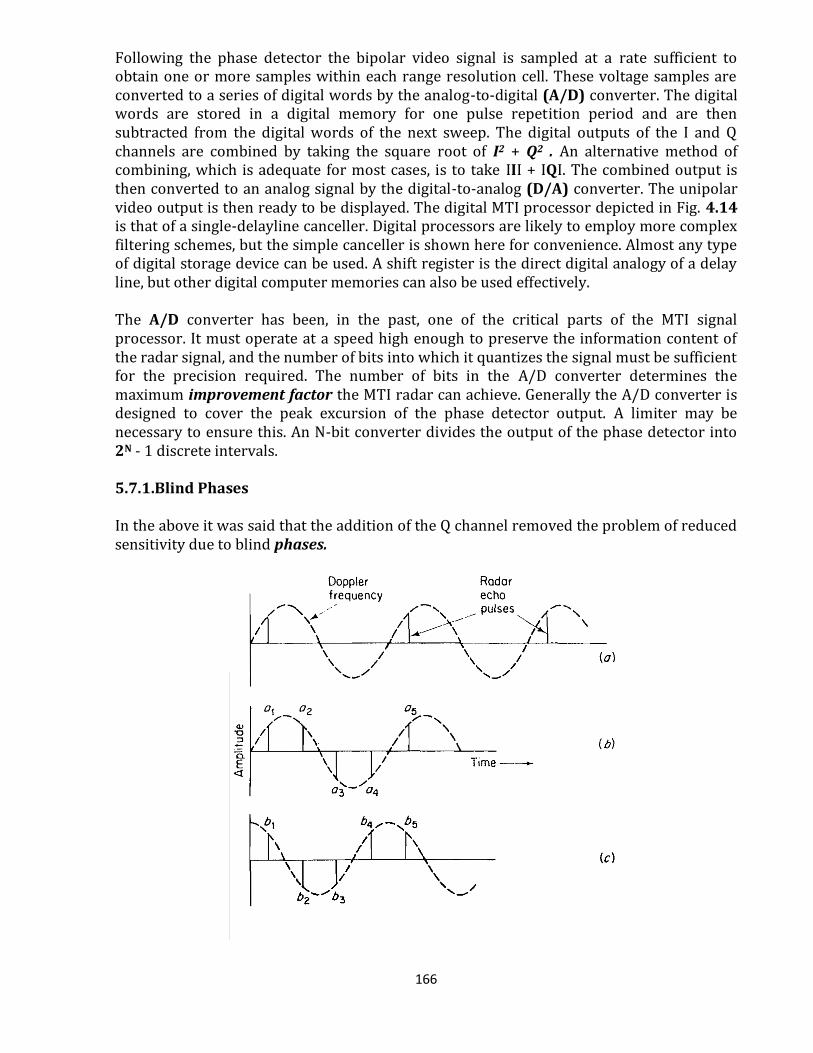
Following the phase detector the bipolar video signal is sampled at a rate sufficient to obtain one or more samples within each range resolution cell. These voltage samples are converted to a series of digital words by the analog-to-digital (A/D) converter. The digital words are stored in a digital memory for one pulse repetition period and are then subtracted from the digital words of the next sweep. The digital outputs of the I and Q channels are combined by taking the square root of I2 + Q2 . An alternative method of combining, which is adequate for most cases, is to take III + IQI. The combined output is then converted to an analog signal by the digital-to-analog (D/A) converter. The unipolar video output is then ready to be displayed. The digital MTI processor depicted in Fig. 4.14 is that of a single-delayline canceller. Digital processors are likely to employ more complex filtering schemes, but the simple canceller is shown here for convenience. Almost any type of digital storage device can be used. A shift register is the direct digital analogy of a delay line, but other digital computer memories can also be used effectively. The A/D converter has been, in the past, one of the critical parts of the MTI signal processor. It must operate at a speed high enough to preserve the information content of the radar signal, and the number of bits into which it quantizes the signal must be sufficient for the precision required. The number of bits in the A/D converter determines the maximum improvement factor the MTI radar can achieve. Generally the A/D converter is designed to cover the peak excursion of the phase detector output. A limiter may be necessary to ensure this. An N-bit converter divides the output of the phase detector into 2N - 1 discrete intervals. 5.7.1.Blind Phases In the above it was said that the addition of the Q channel removed the problem of reduced sensitivity due to blind phases.

167

Figure 4.15 (a) Blind speed in an MTI radar. The target doppler frequency is equal to

the prf. (b) Effect of blind phase in the I channel, and (c) in the Q channel.

This is different than the blind speeds which occur when the pulse sampling appears at the same point in the doppler cycle at each sampling instant, as shown in Fig. 4.15. Figure 4.15 b shows the in-phase, or I, channel with the pulse train such that the signals are of the same amplitude and with a spacing such that when pulse a1 is subtracted from pulse a2, the result is zero. However, a residue is produced when pulse a3, is subtracted from pulse a4, but not when as is subtracted from a4, and so on. In the quadrature channel, the doppler-frequency signal is shifted 900 so that those pulse pairs that were lost in the I channel are recovered in the Q channel, arid vice versa. The combination of the I and Q channels thus results in a uniform signal with no loss. The phase of the pulse train relative to that of the doppler signal in Fig. 4.15 b arid c is a special case to illustrate the effect. With other phase arid frequency relationships, there is still a loss with a single channel MTI that can be recovered by the use of both the I and Q channels. An extreme case where the blind phase with only a single channel results in a complete loss of signal is when the doppler frequency is half the prf and the phase relationship between the two is such that the echo pulses lie on the zeros of the doppler-frequency sine wave. This is not the condition for a blind speed but nevertheless there is no signal. However, if the phase relationship is shifted 900 as it is in the Q channel, then all the echo pulses occur at the peaks of the doppler-frequency sine wave. Thus, to ensure the signal will be obtained without loss, both I and Q channels are desired.

5.7.2. Advantages of Digital Signal Processing Digital signal processing has some significant advantages over analog delay lines, particularly those that use acoustic devices.

It is possible to achieve greater stability, repeatability, and precision with digital processing than with analog delayline cancellers.

The reliability is better. No special temperature control is required, and it can be packaged in convenient

size. The dynamic range is greater since digital MTI processors do not experience the

spurious responses which limit signals in acoustic delay lines. In an analog delay-line canceller the delay time and the pulse repetition period must

be made equal. This is simplified in a digital MTI since the timing of the sampling of the bipolar video can be controlled readily by the timing of the transmitted pulse. Thus, different pulse repetition periods can be used without the necessity of switching delay lines of various lengths in and out. The echo signals for each inter-pulse period can be stored in the digital memory with reference to the time of transmission. This allows more elaborate stagger periods.

The flexibility of the digital processor also permits more freedom in the selection and application of amplitude weightings for shaping the filters.

It has also allowed the ready incorporation of the quadrature channel for elimination of blind phases.

168

In short, digital MTI has allowed the radar designer the freedom to take advantage of the full theoretical capabilities of doppler processing in practical radar systems. 5.8. Limitations to MTI performance The improvement in signal-to-clutter ratio of an MTI is affected by factors other than the design of the doppler signal processor. Instabilities of the transmitter and receiver, physical motions of the clutter, the finite time on target (or scanning modulation), and limiting in the receiver can all detract from the performance of an MTI radar. Before discussing these effects, let us see some relevant definitions

MTI improvement factor: The signal-to-clutter ratio at the output of the MTI system divided by the signal-to-clutter ratio at the input, averaged uniformly over all target radial velocities of interest. Sub-Clutter visibility. The ratio by which the target echo power may be weaker than the coincident clutter echo power and still be detected with specified detection and false alarm probabilities. All target radial velocities are assumed equally likely. A sub-clutter visibility of, for example, 30 dB implies that a moving target can be detected in the presence of clutter even though the clutter echo power is 1000 times the target echo power. Two radars with the same sub-clutter visibility might not have the same ability to detect targets in clutter if the resolution cell of one is greater than the other and accepts a greater clutter signal power; that is, both radars might reduce the clutter power equally, but one starts with greater clutter power because its resolution cell is greater and "sees" more clutter targets. Clutter visibility factor. The signal-to-clutter ratio, after cancellation or doppler filtering, that provides stated probabilities of detection and false alarm. Clutter attenuation. The ratio of clutter power at the canceller input to the clutter residue at the output, normalized to the attenuation of a single pulse passing through the unprocessed channel of the canceller. (The clutter residue is the clutter power remaining at the output of an MTI system.) Cancellation ratio. The ratio of canceller voltage amplification for the fixed-target echoes received with a fixed antenna, to the.

Inter clutter visibility. This describes the ability of MTI radar to detect moving targets which occur in the relatively clear resolution cells between patches of strong clutter. Clutter echo power is not uniform, so if radar has sufficient resolution it can see targets in the clear areas between clutter patches. The higher the radar resolution, the better the inter clutter visibility.

5.8.1.Equipment Instabilities The stability of the equipment in MTI radar must be considerably better than that of ordinary radar. It can limit the performance of MTI radar if sufficient care is not taken in

169

design, construction, and maintenance. The following can cause the apparent frequency spectrum from perfectly stationary clutter to broaden and thereby lower the improvement factor of an MTI radar.

Pulse-to-pulse changes in the amplitude, frequency, or phase of the transmitter signal.

Changes in the stalo or coho oscillators in the receiver, Jitter in the timing of the pulse transmission, Variations in the time delay through the delay lines, and Changes in the pulse width

5.8.2. Internal fluctuation of clutter. Although clutter targets such as buildings, water towers, bare hills or mountains produce echo signals that are constant in both phase and amplitude as a function of time, there are many types of clutter that cannot be considered as absolutely stationary. Echoes from trees, vegetation, sea, rain, and chaff fluctuate with time, and these fluctuations can limit the performance of MTI radar. 5.8.3 Antenna scanning modulation. As the antenna scans by a target, it observes the target for a finite time equal to to = nB/ fp = θB / θs where nB = number of hits received, fp =

pulse repetition frequency, θB, = antenna beamwidth and θs = antenna scanning rate. The received pulse train of finite duration to has a frequency spectrum (which can be found by taking the Fourier transform of the waveform) whose width is proportional to 1/to. Therefore, even if the clutter were perfectly stationary, there will still be a finite width to the clutter spectrum because of the finite time on target. If the clutter spectrum is too wide because the observation time is too short, it will affect the improvement factor. This limitation has sometimes been called scanning fluctuations or scanning modulation. 5.8.4. Limiting in MTI radar. A limiter is usually employed in the IF amplifier just before the MTI processor to prevent the residue from large clutter echoes from saturating the display. Ideally an MTI radar should reduce the clutter to a level comparable to receiver noise. 5.9. Non-Coherent MTI The composite echo signal from a moving target and clutter fluctuates in both phase and amplitude. The coherent MTI and the pulse-doppler radar make use of the phase fluctuations in the echo signal to recognize the doppler component produced by a moving target. In these systems, amplitude fluctuations are removed by the phase detector. The operation of this type of radar, which may be called coherent MTI, depends upon a reference signal at the radar receiver that is coherent with. the transmitter signal. It is also possible to use the amplitude fluctuations to recognize the doppler component produced by a moving target. MTI radar which uses amplitude instead of phase fluctuations is called non-coherent (Fig. 4.16). It has also been called externally coherent, which is a more descriptive name. The non-coherent MTI radar does not require an internal coherent reference signal or a phase detector as does the coherent form of MTI. Amplitude limiting cannot be employed in the non-coherent MTI receiver; else the desired amplitude

170

fluctuations would be lost. Therefore the IF amplifier must be linear, or if a large dynamic range is required, it can be logarithmic. A logarithmic gain characteristic not only provides protection from saturation, but it also tends to make the clutter fluctuations at its output more uniform with variations in the clutter input amplitude.

Fig 4.16: Block diagram of a non-coherent MTI radar.

The detector following the IF amplifier is a conventional amplitude detector. The phase detector is not used since phase information is of no interest to the non-coherent radar. Tile local oscillator of the non-coherent radar does not have to be as frequency-stable as in the coherent MTI. The transmitter must be sufficiently stable over the pulse duration to prevent beats between overlapping ground clutter, but this is not as severe a requirement as in the case of coherent radar. The output of the amplitude detector is followed by an MTI processor such as a delay-line canceller. The doppler component contained in the amplitude fluctuations may also be detected by applying the output of the amplitude detector to an A-scope. Amplitude fluctuations due to doppler produce a butterfly modulation similar to that in Fig. 4.3, but in this case, they ride on top of the clutter echoes. Except for the inclusion of means to extract the doppler amplitude component, the non-coherent MTI block diagram is similar to that of a conventional pulse radar. 5.9.1. Advantages and limitations of non-coherent radar The advantage of the non-coherent MTI is its simplicity; hence it is attractive for those applications where space and weight are limited. Its chief limitation is that the target must be in the presence of relatively large clutter signals if moving-target detection is to take place. Clutter echoes may not always be present over the range at which detection is desired. The clutter serves the same function as does the reference signal in the coherent MTI. If clutter were not present, tlie desired targets would not be detected. It is possible, however, to provide a switch to disconnect the non-coherent MTI operation and revert to normal radar whenever sufficient clutter echoes are not present. If the radar is stationary, a map of the clutter might be stored in a digital memory and used to determine when to switch in or out the non-coherent MTI. The improvement factor of a non-coherent MTI will not, in general, be as good as can be obtained with a coherent MTI that employs a reference oscillator (coho). The reference signal in the non-coherent case is the clutter itself, which will not be as stable as a reference oscillator because of the finite width of the clutter

171

spectrum caused by its own internal motions. If a nonlinear IF amplifier is used, it will also limit the improvement factor that can be achieved.

5.10. Pulse Doppler Radar A pulse radar that extracts the doppler frequency shift for the purpose of detecting moving targets in the presence of clutter is either an MTI radar or a pulse doppler radar. The distinction between them is based on the fact that in a sampled measurement system like a pulse radar, ambiguities can arise in both the doppler frequency (relative velocity) and the range (time delay) measurements. Range ambiguities are avoided with a low sampling rate (low pulse repetition frequency), and doppler frequency ambiguities are avoided with a high sampling rate. However, in most radar applications the sampling rate, or pulse repetition frequency, cannot be selected to avoid both types of measurement ambiguities. Therefore a compromise must be made and the nature of the compromise generally determines whether the radar is called an MTI or a pulse doppler. MTI usually refers to a radar in which the pulse repetition frequency is closely low enough to avoid ambiguities in range (no multiple-time-around echoes) but with the consequence that the frequency measurement is ambiguous and results in blind speeds, Eq. (4.8). The pulse doppler radar, on the other hand, has a high pulse repetition frequency that avoids blind speeds, but it experiences ambiguities in range.

The pulse doppler radar is more likely to use range-gated doppler filter-banks than delay-line cancellers. Also, a power amplifier such as a klystron is more likely to be used than a power oscillator like the magnetron. A pulse doppler radar operates at a higher duty cycle than does an MTI. Although it is difficult to generalize, the MTI radar seems to be the more widely used of the two, but pulse doppler is usually more capable of reducing clutter. Even so, the pulse-doppler radar has an advantage over the CW radar in that the detection performance is not limited by transmitter leakage or by signals reflected from nearby clutter or from the radome. The pulse-doppler radar avoids this difficulty since its receiver is turned off during transmission, whereas the CW radar receiver is always on. On the other hand, the detection capability of the pulse-doppler radar is reduced because of the blind spots in range resulting from the high prf.

*****

Solved Problems

1. Define blind speed. An MTI Radar operates at 5 GHz with PRF of 100 pps. Find the 3 lowest

blind speeds of this Radar. Explain the importance of staggered PRFs. [JNTU May 2013]

vn = 𝒏𝝀𝒇𝒑

𝟐 n = 0, 1, 2, . . .,

λ = c/f = 3 x 108 / 5 X 109 =0/06 m

v1 = 𝝀𝒇𝒑

𝟐 =

𝟎.𝟎𝟔 𝒙 𝟏𝟎𝟎

𝟐 = 3 m/s

Similarly v2= 6 m/s, v3 = 9 m/s

172

2. Determine the first three blind speeds of MTI radar operating at a frequency of 10 GHz

with PRF of 1 kHz.

For f= 10 G Hz, 𝜆 = .03 𝑚

vn = 𝒏𝝀𝒇𝒑

𝟐 n = 0, 1, 2, . . .

v1 = 𝝀𝒇𝒑

𝟐 =

𝟎.𝟎𝟑 𝒙 𝟏𝟎𝟎𝟎

𝟐 = 15 m/s

Similarly v1 = 30 m/s, v3 = 45 m/s

3. An MTI radar is operated at 9GHz with a PRF of 3000 pps. Calculate the first two lowest blind speeds for this radar. Derive the formula used. [JNTU May 2011]

For f= 9 G Hz, 𝜆 = .033 𝑚

vn = 𝒏𝝀𝒇𝒑

𝟐 n = 0, 1, 2, . . .

v1 = 𝝀𝒇𝒑

𝟐 =

𝟎.𝟎𝟑𝟑 𝒙 𝟑𝟎𝟎𝟎

𝟐 = 49.5 m/s

Similarly v2 = 99 m/s,

Essay type questions

1. What is MTI Radar? How does it operate?[JNTU May 2013] 2. Compare MTI radar with Pulse Doppler Radar. [JNTU May 2013] 3. Explain the function of single delay line canceller and derive an expression for the

frequency response function. [JNTU May 2013] 4. Discuss about the internal fluctuation of clutter which limits the performance of MTI

Radar. [JNTU May 2012] 5. Describe briefly the analog MTI systems. [JNTU May 2012] 6. With block diagram explain MTI radar using range gated doppler filters. 7. Differentiate blind phases from blind speeds. [JNTU May 2012] 8. What is the method of overcoming the problems of blind speed in analog radars? [JNTU

May 2012] 9. What is the need of delay line canceller? Explain three pulse canceller. [JNTU May 2012] 10. Explain how the bipolar video signal is converted in to unipolar signal in MTI

radar that uses range gates and filters. [JNTU May 2012] 11. Derive an expression for blind speeds of MTI radar. Discuss the effect of large

wavelength and large PRF on lowest blind speed of target. [JNTU May 2012] 12. Differentiate blind phases from blind speeds. [JNTU May 2011] 13. Discuss the various types of MTI delay lines used in MTI radar. [JNTU May 2011] 14. Draw the output waveforms from mixer for the different range of Doppler frequency.

[JNTU May 2011] 15. Write short notes on inter clutter visibility, MTI improvement factor and clutter

attenuation. [JNTU May 2011] 16. Explain the limitations of MTI Radar. [JNTU May 2011]

173

17. Explain how the effects of blind speeds reduced by operating at more than one PRF? [JNTU May 2011] 18. Discuss the limitations of non-coherent MTI Radar systems. [JNTU May 2011] 19. Mention the limitations of MTI radar related to clutter parameters. [JNTU May 2010] 20. Mention the limitations of improvement factor imposed by pulse-to-pulse in-stability.

[JNTU May 2010] 21. Write short notes on inter clutter visibility. [JNTU May 2010] 22. Explain the operation of an MTI radar with 2 prfs. [JNTU May 2010] 23. Draw the block diagram of Range-Rated Doppler Filters and explain. [JNTU May 2010] 24. Mention the limitations of MTI radar related to clutter parameters. [JNTU May 2010] 25. Mention the limitations of improvement factor imposed by pulse-to-pulse in-stability. [JNTU May 2010] 26. Write short notes on inter clutter visibility. [JNTU May 2010] 27. Explain the operation of an MTI radar with 2 prfs. [JNTU May 2010] 28. Draw the block diagram of Range-Rated Doppler Filters and explain. [JNTU May 2010] 29. Discuss the filter characteristics of the delay line canceller? [JNTU Jan 2010] 30. Draw the block diagram of a delay line filter which produces a 3-pole Chebyshev low

ass filter characteristic with 0.5db ripple in the passband? [JNTU Jan 2010] 31. Write about the following: [JNTU Jan 2010]

(i) Blind speeds (ii) staggered prf. 32. Explain the principle of operation of MTI radar with power amplifier transmitter with neat

block diagram. [JNTU May 2009] 33. What is butterfly effect? What are its advantages. [JNTU May 2009] 34. Explain the principle of operation of MTI radar with power oscillator transmitter with neat

block diagram. [JNTU May 2009] 35. Discuss about blind speeds. [JNTU May 2009] 36. Discuss about staggered pulse repetition frequencies. [JNTU May 2009] 37. Explain the principle of operation of MTI radar using range gates and filters. [JNTU May

2009] 38. Write notes on the following: [JNTU May 2009]

i) Delay line cancellers

ii) Blind speeds

iii) Clutter attenuation

iv) Transversal filters.

Objective type questions

1. One method commonly employed to extract Doppler information in a form suitable for display on the PPI scope is with a a. Power Amplifier b. A-Scope display

c. Delay line canceller d. Coherent oscillator 2. The characteristic feature of coherent MTI Radar is that the

a. Transmitted signal must be out of phase with reference signal in receiver b. The transmitted signal must be equal in the magnitude with reference signal c. The transmitted signal must be coherent with the reference signal in the receiver d. Transmitted signal must not be equal to reference signal in the receiver

174

3. In the following which are produce, with time a butterfly effect on the 'A' scope a. Fixed Targets b. PPI scope c. Moving Targets d. Phase Detector

4. The stalo, coho and the mixer in which they are combined plus any low-level amplification are called the

a. Transmitter-Oscillator b. Transmitter-Exciter c. Receiver-Amplifier d. Receiver-exciter

5. The Doppler frequency shift produced by a moving target may be used in a pulse radar to

a. Combine moving targets from desired stationery objects b. Determine the relative velocity of a target c. Separate desired moving targets from desired stationery objects d. Determine the displacement of a target

6. To operate with unambiguous Doppler pulse repetition frequency is usually

a. Low b. Very low c. High d. Very High 7. MTI stands for

a. Moving Transmitter Indicator b. Moving target interval c. Moving target indication d. Modulation Transmitting Interval

8. Echoes from fixed targets

a. Vary in amplitude b. Vary in frequency c. Vary in pulse interval d. Remains constant

9. The limitation of pulse MTI radar which do not occur with CW radar

a. Blind speeds b. Delay lines c. Requires more operating powers d. requires complex circuitry

10. The presence of blind speeds within the Doppler frequency band reduces the

a. Output of the radar b. Detection capabilities of the radar c. Unambiguous range d. Ambiguous range

11. The capability of delay line canceller depends on the

a. Quality of signal b. Pulse Interval c. Quality of the medium used d. Delay time of the delay line

12. The output of the MTI receiver phase detector be quantized into a sequence of digital words by using

a. Digital quantizer b. Digital Phase detector c. Digital delay lines d. Digital filter

13. A transmitter which consists of a stable low power oscillator followed by a power amplifier is called a. POMA b. MOPA c. MTI Radar d. CW radar 14. A simple MTI delay line canceller is an example of a

175

a. Frequency domain filter b. High pass filter c. Active filter d. Time domain filter

15. The delay line must introduce a time delay equal to the

a. Time interval b. Pulse repetition interval c. Pulse width d. Phase shift

16. The delay line canceller

a. Rejects the ac component of clutter b. Rejects the dc component of clutter c. Allows the ac as well as dc d. It rejects all components

17. In pulse MTI radar, Doppler is measured by

a. Continuous signals b. Discrete samples c. Constant period d. Constant amplitude

18. The output of the two single delay line cancellers in cascade is the

a. Double of that from a single canceller b. U times that from a single canceller c. Square of that from a single canceller d. Same as that from a single canceller

19. To operate MTI radar with high pulse repetition frequencies

a. λ fp must be small b. λ fp must be unity

c. λ fp must be zero d. λ fp must be large

20. If the first blind speed were 600 knots, the maximum unambiguous range would be ----- at a frequency of 300MHz

a. 140 nautical miles b. 600 knots c. 140 knots d. 130 nautical miles

21. The maximum unambiguous range

a. Runamb = cT/2 b. Runamb = (cT)2 c. Runamb = cT/4 d. Runamb = (cT/2)2

22. To operate MTI radar at low frequencies

a. λ fp must be small b. λ fp must be zero

c. λ fp must be large d. λ fp must be unity

23. The effect of blind speed can be significantly reduced in

a. Pulse MTI radar b. Delay line canceller c. Staggered - prf MTI d. Pulse canceller

24. The blind speeds are present in pulse radar because

a. Doppler is measured by discrete samples at the prf b. Doppler is measured by continuous signal c. Doppler is assumed to be zero d. Doppler frequency remains constant

25. If the first blind speed is to be greater than the maximum radial velocity expected

176

from the target, the product λ fp must be a. Small b. Zero c. Large d. Infinity

26. The clutter-rejection notches may be widened by passing the output of the delay line canceller through a

a. Coho b. Stalo c. Second delay line canceller d. Pulse canceller 27. The frequency response of double delay line canceller is

a. 4 Sin nfdT b. 4 π Sin nfdT c. 4 Sin2 nfdT d.(2π Sin nfdT)2 28. MTI radar primarily designed for the detection of aircraft must usually operate with

a. Unambiguous Doppler b. Unambiguous blind speed c. Ambiguous Doppler d. Ambiguous range

29. The blind speeds of two independent radars operating at the same frequency will be different if their

a. Amplitudes are different b. Blind speeds are different c. Pulse repetition frequencies are different d. Puse intervals are different

30. A disadvantage of the staggered prf is its inability to

a. Cancel second-time around echoes b. Cancel second-time around clutter echoes c. Provide variable prf d. Provide pulse to pulse incoherence

31. Second-time around clutter echoes can be removed by use of a

a. Stalo b. Coho c. Constant prf d. Delay canceller 32. The loss of range information and the collapsing loss may be eliminated by

a. Sampling the range b. Shaping the rangec. Quantizing the range d. Keeping constant range

33. Range gating is a process of

a. Sampling the range into various samples b. Quantizing the range into small intervals c. Getting constant range d. Removing the range intervals

34. When the switching is pulse to pulse. It is known as a

a. Delay canceller b. Staggered prf c. MTI radar d. Pulse radar

35. Pulse to pulse coherence is provided by use of

a. Stalo b. Coho c. Constant prf d. Delay canceller 36. The output of the range gates is stretched in a circuit called

a. Clutter rejection filter b. Clutter filter

177

c. Box car generator d. Sampler 37. The clutter rejection filter is a

a. Band stop filter b. Bandpass filter c. Lowpass filter d. Highpass filter

38. The bandwidth of clutter rejection filter depends upon the extent of the

a. Spectrum b. Expected clutter spectrum c. Filter characteristic d. Clutter characteristic

39. By quantizing the range

a. Loss of range Information is eliminated b. Loss of range information is increased c. Range becomes constant d. Range becomes sampled

40. Clutter visibility factor provides

a. Attenuation b. Probabilities of detection and false alarm c. Cancellation ratio d. Decrease in clutter residue

41. In box car generator

a. Output of range gates is quantized b. Output of range gates is sampled c. Output of range gates is stretched d. Range gate output remains constant

42. The clutter power remaining at the output of MIT system is

a. Clutter pulse b. Clutter residue c. Clutter Attenuation d. Clutter power ratio

43. Amplitude limiting cannot be employed in

a. Coherent MTI receiver b. Pulse Doppler radar c. Non-coherent MTI receiver d. CW radar

44. It provides stated probabilities of detection and false alarm

a. Clutter attenuations b. Clutter ratio c. Cancellation ratio d. Clutter visibility factor

45. MTI radar which uses amplitude fluctuations is

a. Coherent b. Pulsed Doppler c. Non coherent d. CW radar

46. Constant prf is helpful to provide

a. Pulse to pulse coherence b. Stalo c. Delay d. Coho

Radar Systems

Unit-V: MTI Radar Page 50

47. Clutter residue is

a. Clutter input power b. Clutter power remaining at output of MTI system

c. Clutter output power ratio d. Clutter output attenuation

48. By using constant prf

a. Clutter factor is minimized b. Clutter input power is increased

c. Clutter echoes can be removed d. Range gate output can be sampled

Answers Q A Q A Q A Q A Q A Q A Q A

1 C 2 D 3 C 4 D 5 B 6 C 7 C

8 D 9 A 10 B 11 C 12 C 13 B 14 D

15 B 16 B 17 B 18 C 19 D 20 D 21 A

22 C 23 C 24 A 25 C 26 C 27 C 28 C

29 C 30 B 31 C 32 C 33 B 34 B 35 C

36 C 37 B 38 B 39 A 40 B 41 C 42 B

43 C 44 D 45 C 46 A 47 B 48 C