universitÀ degli studi di padova - benvenuti su padua@thesis -...
TRANSCRIPT

UNIVERSITÀ DEGLI STUDI DI PADOVA
DIPARTIMENTO DI INGEGNERIA CIVILE EDILE ED AMBIENTALE- DICEA
Laurea Magistrale in ingegneria Civile
Tesi magistrale/ Master Thesis:
From masonry to reinforced concrete arch bridges:
load capability and seismic analysis
Relatore/ Supervisor: Chiar.mo Prof. Ing. Carlo Pellegrino
Correlatore/Assistant Supervisor: Daniel V. Oliveira
Laureanda/ Student: Chiara Magnani
ANNO ACCADEMICO 2014-2015


From masonry to RC arch bridges: load capability and seismic analysis
I Master Thesis
To my family which always gave me the strength
and the perseverance to believe and obtain my purposes.

From masonry to RC arch bridges: load capability and seimsic analysis
II Master Thesis
Alla mia famiglia che mi ha sempre dato la forza
e la perseveranza per credere e raggiungere i miei obiettivi.

From masonry to RC arch bridges: load capability and seismic analysis
III Master Thesis
ACKNOWLEDGEMENTS
I wish to thank Professor Daniel Oliveira for his teaching, supervision and immense support during my
stay in University of Minho. He always greeted me with a smile and a good word, that being far from
home, was always an great encouragement for me.
I’m grateful also to Minho University because offered to me the opportunity to live a good and useful
experience.
Finally, I want to thank Professor Carlo Pellegrino, who followed me also for my first thesis and has
been always an helpful and important teacher.
Thanks to the University of Padua for these years.
This thesis has been elaborated at University of Minho, Guimarães (Portugal), thanks to Erasmus
program 2014/2015.

From masonry to RC arch bridges: load capability and seismic analysis
IV Master Thesis

From masonry to RC arch bridges: load capability and seismic analysis
V Master Thesis
ABSTRACT
In this essay arch bridges are studied. Starting from historical masonry arch bridges till concrete ones,
their features are considered. In particular Durrães Viaduct is examined and a new poposal of the bridge
in reinforced concrete is offered. The structure is analysed under dynamic aspects with fibre beam
modelling, that is chosed for its accuracy in numerical results althought the simplicity of a 1-D model.
For this reason a careful presentation of fibre element theory is done and of the different analysis
implemented in this work.

From masonry to RC arch bridges: load capability and seismic analysis
VI Master Thesis
RIASSUNTO
Nel presente elaborato sono studiati ponti ad arco; partendo da i primi ponti ad arco in murature fino a
quello più recenti in cemento. In particolare, il viadotto di Durrães viene analizzato e una proposta di
nuovo ponte in cemento armato è offerta. La struttura, viene esaminata dal putno di vista dinamicoper
mezzo di una modellazione a fibre, la quale è stata scelta per il suo grado di accuratezza nonostante si
tratti di una modellazione monodimensionale.Proprio per questa ragione, nella presente tesi, viene
riportata anche un’ attenta presentazione della teoria delle fibre e dei differenti metodi di analisi
adottati in questo lavoro.
From masonry to RC arch bridges: load capability and seismic analysis
VII Master Thesis
INDEX
1 INTRODUCTION 1
1.1 Motivation and scopes 1
1.2 Organization of the work 1
2 HISTORICAL ARCH BRIDGES 3
2.1 Historical overview 3
2.2 Constitutive elements of masonry arch bridges 4
2.3 Elements of the bridge design- historical data and empirical rules 5
2.3.1 Shape of the arch 6
2.3.2 Thickness of the arch 8
2.3.3 Width of the pier 9
2.3.4 Load mechanism transmission in arches 10
2.3.5 Failure mechanism in arches 11
2.3.6 Damages on historical masonry Arch Bridges 12
2.4 Concrete Arch Bridges 14
3 A MODELLING BASED ON FIBRE ELEMENTS 17
3.1 Beam element formulation 17
3.2 SeismoStruct: Main features 26
3.3 Analysis type 30
3.4 Modelling test of a small concrete bridge 35
3.4.1 Bolton experimental laboratory bridge 35
3.4.2 Bolton Bridge reinforced concrete: load-carrying capability 38
4 SEISMIC PERFORMANCE OF A RC ARCH BRIDGE 47
4.1 Durrães Viaduct 47
4.1.1 Historical Overwiev 47
4.1.2 Load-Carrying capability of Durrães 50

From masonry to RC arch bridges: load capability and seismic analysis
VIII Master Thesis
4.1.3 Durrães viaduct actual damages 52
4.2 Alternative new solution for Durrães 54
4.2.1 New Reinforce Concrete Durrães bridge 54
4.3 Non-Linear structural Analysis 59
4.3.1 Load-carrying Capability 59
4.3.2 Push-over Analysis 62
4.4 Non-linear dynamic analysis 71
4.4.1 Numerical modal analysis 71
4.4.2 Seismic Input 73
4.4.3 Analysis setting and parameters 77
4.4.4 Time-history analysis 81
4.4.5 IDAs results and comparison with Pushover 84
5 CONCLUSIONS AND FUTURE WORKS 87
5.1 Conclusions 87
5.2 Future development opportunities 89
REFERENCES 91
APPENDIX A 95
APPENDIX B 103

From masonry to RC arch bridges: load capability and seismic analysis
IX Master Thesis
List of Figures
Figure 2.1: Elements of multi-span masonry arch bridges (Lourenço, et al., 2007) 4
Figure 2.2: Empirical rules for the design of arch from Mery and Alberti (De Santis, 2011), (Proske, et al., 2009) 5
Figure 2.3: Empirical relations for the design of structural elements of a bridge (FSI, 1907). (De Santis, 2011) 6
Figure 2.4: Types of arch geometries (Proske, et al., 2009) 7
Figure 2.5: S. Trinità Bridge (basket arches) 1569, Florence, Italy 7
Figure 2.6: Relationship between span s(m) and rise to span ratio (r/s). 8
Figure 2.7: Relationship between thickness and span ratio (t/s) and span s(m) 9
Figure 2.8: Relationship between pier width and span ratio(P/s) and span s(m) and thickness (m) ,empirical rules
and real bridges. 10
Figure 2.9: Scheme of loads transmission: (a) longitudinal direction, (b) transversal direction (da Cruz Morais,
2012) 11
Figure 2.10: Thrust line collapse in masonry arch (Gilbert, 2007) 12
Figure 2.11: Three example of potential failure mode (Gilbert, 2007) 12
Figure 2.12: Most frequent damages found on masonry arch bridges according to Angeles-Yáñez and Alonso
(Proske, et al., 2009) 13
Figure 2.13: Bridge Km-23, Tehran-Qom Railway (Marefat, et al., 2004) 15
Figure 2.14: Valle-di-Pol bridge (Zanardo, et al., 2004) 15
Figure 2.15: London Bridge in 1870 (various, 2014) and Lake Havasu City London Bridge in 2004 (2004) 16
Figure 2.16: New Saale Bridge South Jena (Proske, et al., 2009) 16
Figure 3.1: lumped plasticity and distributed plasticity elements 17
Figure 3.2: A fibre beam element with its cross section and components’ constitutive laws ( (SeismoStruct, version
7) 18
Figure 3.3: Different constitutive laws between confined and not-confined concrete 18
Figure 3.4: Schematic illustration of state determination at the structure, element and section level (Spacone,
1992) 21
Figure 3.5: Equilibrium of frame element in the deformed configuration and its projection on the undeformed
configuration (De Santis, 2011) 24
Figure 3.6: Points of integration in the Gauss scheme: positions and weight (Viesi, 2008) 27
Figure 3.7: NR ad mNR algorithm 28
Figure 3.8: Static Pushover analysis, fundamental phases (Da Porto, et al., 2013) 32
Figure 3.9: Load-displacement curve obtained with a pushover analysis and displacement corresponding to some
accelerograms. 32
Figure 3.10: two different possible load distribution for pushover 32
Figure 3.11: accelerogram example, acceleration curve depending on time 33
Figure 3.12: Bolton Institute experimental model, case with detached spandrel walls from arches (Professor C.
Melbourne, et al., 1997) 35

From masonry to RC arch bridges: load capability and seismic analysis
X Master Thesis
Figure 3.13: Geometry of the bridge (mm) and load disposition (De Felice, 2009) 36
Figure 3.14: Failure hinged mechanism of laboratory model with corresponding load (De Santis, 2011) 37
Figure 3.15: Load-capability vs. displacement: 37
Figure 3.16: con_ma constitutive law, confined concrete with c.f.=1.2 and steel stl_bl constitutive law 39
Figure 3.17: Bolton reinforced concrete: Vault section 40
Figure 3.18: Bolton reinforced concrete: Pier section 40
Figure 3.19: Model features, meshing, permanent and incremental load disposition 41
Figure 3.20: Diffusion of the load from the trampling level to the arch extrados and identification of the loaded
nodes. 41
Figure 3.21: 1.Compression concrete constitutive law and compression concrete performance criteria (black
point)
2.Tensile concrete constitutive law and tensile performance criteria (light green and dark green points) 42
Figure 3.22: Load-displacement response referred to node B11, point of application of external load. The six
coloured point stay for performance criteria. 43
Figure 3.23: Plasticity mechanism development, deformed shapes and performance criteria 44
Figure 3.24: Last deformed shape before collapse and element most loaded 44
Figure 3.25: Respectively: Fiber1,Fiber2 for concrete (confined and unconfined), Fiber3 for concrete stretched and
Fiber4 for steel: (green elements) 45
Figure 3.26: Strain-stress relation for Fiber1 and Fiber2, most compressed concrete fibres (confined or
unconfined) 45
Figure 3.27: (a)Strain-Stress relation for Fiber3 46
Figure 4.1: Durrães viaduct and binary detail 47
Figure 4.2: Durrães bridge structure 48
Figure 4.3: Potential relative movements between blocks (simple LP limit analysis model) (Gilbert, 2007) 50
Figure 4.4: Most conservative collapse behaviour 51
Figure 4.5: (a) local, (b)semi-global and (c) global mechanism of collapse 51
Figure 4.6:(a)Spandrel wall between the third and fourth arch with vegetation contamination. 52
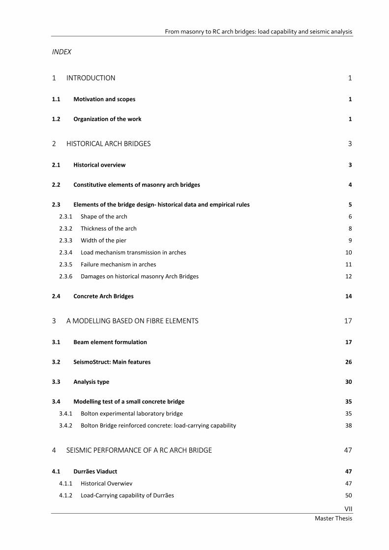
Figure 4.7: New concrete bridge structure, sections and particular arch-pier 55
Figure 4.8: Materials constitutive laws- concrete C30/37 and reinforcement B500A 56
Figure 4.9: Arches and pier discretization; modelling features. 57
Figure 4.10: constitutive laws for concrete and steel: performance criteria points 58
Figure 4.11: Nodal incremental load disposition used in the time history analysis 59
Figure 4.12: Load-carrying capability curve, node most exposed to direct live load 60
Figure 4.13: Deformed shape (15% scale) and performance criteria for step (1), (2), (3) of Figure 4.12. 61
Figure 4.14: Spandrel wall and infill soil masses disposition on an arch segment 63
Figure 4.15: Selected nodes for pushover capability curves 64
Figure 4.16: Pushover curves for Control Nodes (cN) selected in X direction 64
Figure 4.17: Pushover curve in positive X direction for control Node 1 65

From masonry to RC arch bridges: load capability and seismic analysis
XI Master Thesis
Figure 4.18 (1): deformed shape (15% scale) of step (1) and performance criteria 65
Figure 4.19 (a): compression (cc) and tension (ct) in concrete fibres 67
Figure 4.20: Pushover curves for Control Nodes (cN) selected in X direction 68
Figure 4.21: (a) Pushover curve in positive Y direction for control Node- (b)Last deformed shape for α=1.0 68
Figure 4.22(1)’-(2)’: deformed shape (15% scale) of steps (1)’-(2)’ and performance criteria 69
Figure 4.23: strain-stress curves in concrete and steel in three important fibres 70
Figure 4.24: Deformed shape of the first two modes in X and Y direction. 72
Figure 4.25: Figure NA.I (CEN, 2010). Seismic zoning for continental Portugal 73
Figure 4.26: Elastic accelerogram and displacement spectra-type1 and type2 75
Figure 4.27: three accelerograms generated from spectrum-2, PGA/g=0.0816 76
Figure 4.28: Comparison between artificial spectra and Eurocode specified spectra (type2). 76
Figure 4.29: Stiffness proportional damping coefficient distribution adopted. 79
Figure 4.30: (a) hysteretic curves and displacement trend for cN1, (b) hysteretic curves zoom- SF=1.0 81
Figure 4.31: deformed shape for the most heavy damage for PGA1 82
Figure 4.32: (a) Hysteretic curve for 1PGA-2PGA-4PGA vs. pushover; (b) displacement-time trend (cN1) 82
Figure 4.33: Deformed shapes for 2PGA and 4PGA 83
Figure 4.34: (a) Hysteretic curve for 6PGA-8PGA-10PGA vs. pushover; (b) displacement-time trend (cN1) 83
Figure 4.35: Deformed shapes for 6-8-10 PGA 84
Figure 4.36: Incremental dynamic values for the three accelerograms 85
Figure 4.37: IDA curve for average values of the three accelerograms 86

From masonry to RC arch bridges: load capability and seismic analysis
XII Master Thesis
List of Tables
Table 2.1: Different empirical thickness arch formulas (Oliveira, et al., 2010) 9
Table 2.2: Historical empirical rules for the thickness of the pier top from different author (De Santis, et al., 2014)
10
Table 2.3: Masonry railway arch bridges repairing activities according to Orbán (Proske, et al., 2009) 14
Table 3.1: Input and output data for each module of the state determination process. 22
Table 3.2: Non linear analysis for seismic action by EC8 30
Table 3.3: Geometric and mechanical characteristics of Bolton Institute experimental model (Professor C.
Melbourne, et al., 1997) 36
Table 3.4: Parameters describing the behaviour of the con_ma concrete material 38
Table 3.5: Parameters describing the behaviour of the stl_bl steel material 39
Table 3.6: Section characteristics of the reinforced concrete vault 40
Table 3.7: Section characteristics of reinforced concrete pier 40
Table 3.8: Colours referred to each performance criteria, name and relative strain 42
Table 3.9: Displacement-Load of points (A)-(F) 43
Table 4.1:Geometry of Durrães bridge 48
Table 4.2: Masonry and infill mechanical properties of Durrães viaduct (Oliveira, et al., 2014) 49
Table 4.3: Dimension of new concrete Bridge 55
Table 4.4: mechanical properties of materials 56
Table 4.5: performance criteria: name, strain value and colour notification related 58
Table 4.6: First two modes in X and Y direction and important parameters 72
Table 4.7: Seismic parameters for Barcelos 74
Table 4.8: IDA values of displacement, forces and shear factor and relative average values 85
Table 4.9: Comparison between pushover and IDA values of displacements, base shear and shear factor. 86

From masonry to RC arch bridges: load capability and seismic analysis
XIII Master Thesis

From masonry to RC arch bridges: load capability and seismic analysis
XIV Master Thesis

Introduction
1 Master Thesis
1 Introduction
1.1 Motivation and scopes
The present study started from the interest in old arch multispan bridges that constitute a precious
heritage, from the 19th century until modern times, for the entire Europe.
It is important to examine their features, understand their behaviour and eventually to intervene in casa
that these structure do not assure a great level of safety condition of loads and the actual legislations,
that request more restrictive characteristics.
A brief treatment about the historical features of masonry arch bridges, till concrete ones and their
problem is necessary to understand the behaviour of these typology of structure and their mechanism
of collapse. Given that the last part of the work presents a study of a concrete arch bridge and its
modelling, the interest is also to decide how to model this viaduct and which theory stands at the base
of this numerical analysis. The choice to operate with a fibre software seems the most convenient,
because guarantees simplicity, lightness of computational contribution, and high performances taking
into account the distinct material properties.
In particular the aim of this work is to propose a modern solution of bridge, starting from the old viaduct
of Durrães, positioned in the North of Portugal and exactly in Barcelos (Braga). Considering the beauty
of the valley where the bridge is situated and the importance to preserve the historical appearance of
the area, the modern reinforced concrete bridge proposed is a multispan arch bridge as the ancient one
and presenting the same general characteristics. Consequently to a short analysis on the masonry
Durrães viaduct, the new bridge is presented and on it several numerical analysis are provided.
In the following section the organization of the work is presented.
1.2 Organization of the work
The thesis is organized in five chapters:
Chapter1: Introduces the topics of the study, the objectives and the organization of the essay
Chapter2: Presents a historical overview of the type of structure discussed in the thesis, the features
and the old methodology of design. Survey studies are reported for masonry old bridges. In the last
part concrete arch bridges are introduced.

From masonry to RC arch bridges: load capability and seismic analysis
2 Master Thesis
Chapter3: The theory of fibres element modelling is explained in detail, because the consecutive
numerical analysis are based on this construct and all input data refer to the definitions given in this
chapter. It is explained also the software features and the type of analysis available. Finally a numerical
test is done on the laboratory model made in Bolton University (Professor C. Melbourne, et al., 1997),
to presents how the software works and some evaluations on the differences between masonry and
concrete results.
Chapter4: Here the Durrães viaduct is considered. The old masonry bridge is presented with its
characteristics and its damages. The capability of the bridge is assessed by a static limit analysis done
by means of the software LimitRing. After this, the reinforced concrete new bridge is introduced, with
its geometrical and material features. The last part of the chapter considers the modern viaduct and its
numerical modelling. The numerical simulations concern semi-static vertical loading, pushover
analysis, non-linear time history analysis and incremental dynamic analysis under three different
accelerograms.
Chapter5: The conclusions of the work are drawn with some sparks for possible future works.

Historical arch bridges
3 Master Thesis
2 Historical arch bridges
2.1 Historical overview
The European railway system constitutes a precious cultural heritage, comprising the several numbers
of masonry arch bridge, considering small single-span bridges to large multi-span viaduct.
Most of them was built in a lapse of one hundred years, approximately since the second half of 19th
century until the first half of the 20th, and even if geographical position, materials, dimensions could
change, it is easy to recognize similar structural features and design techniques.
There are a lot of treatises or manuals of 18th, 19th and 20th Centuries about traditional building rules,
dating from 80 to almost 300 years ago, and moreover several old design instructions such as FSI
(Ferrovie dello Stato Italiano, 1907) in the first Italian National Technical Code,emitted by the Italian
Railway Institution. In some cases, empirical concept were used, based on practical optimization of
previous creations. Furthermore, graphical methods were employed for deriving the better line of the
arch.
The expected traffic loads were lower than the actual ones and the seismic action was not explicitly
included in the calculations; moreover, material degradation processes, foundation settlements,
structural damages, transformations or partial demolitions could have occurred with the passing of
time.
At present time, an accurate assessment towards both traffic and earthquake loads is necessary
according to the safety standard requested by actual codes.
It is now necessary, and of great interest as well, to manage specialized analysis and intervention
methodologies to ensure the safety level of existing masonry bridges towards actual traffic loads using
the tools of present time. In some other case, if the existing structure is irreparable and also with
refurbishment does not guarantee a satisfying level of safety it is necessary to replace the old bridge
with a new one. Sometimes, it is also necessary, for an heritage conservation reason, to maintain also
the previous aspect, working with different and modern materials that present higher performances.
Thanks to the new procedures of analysis, a satisfactory compromise between accuracy and simplicity
is possible performing reliability and design interventions, but researchers have to face the challenge
of developing tools aiming to the best application of them. A well-founded structural model has to
include, among the other things, an accurate description of the material properties and of the effect
induced by the interaction between structural elements on the whole response. Moreover, an adequate

From masonry to RC arch bridges: load capability and seismic analysis
4 Master Thesis
representation of the external actions has to be provided and computational sustainability and
robustness, as well as clearness and simplicity in the determination of the parameters, have to be
ensured. Since the professional utilization asks for low modelling and calculus time, and
comprehensible, verifiable and, of course, reliable results.
Several researches are carried on to deepen the knowledge and valorisation of historical construction,
examining or simply collecting and rediscovering historic design rules and construction technologies,
or surveying the most recurrent typologies and geometrical properties of ancient bridges in a particular
geographic area (Oliveira et al., 2010).
In this chapter some fundamental information about arch bridges are exposed, starting from masonry
until concrete bridges. In particular, the geometrical features, the type of damages and the behaviour
of these structures are considered in the present chapter.
2.2 Constitutive elements of masonry arch bridges
Generally, arch masonry bridges present common composition in which it is possible to define some
essential and recurring elements composing the structure and better reported in Figure 2.1. The bridge
geometry is primarily conditioned by the valley’s to cross orography an when this is considerable deep,
the crossing bridge may present multi-span and high piers characteristic and in that case it is possible
to define a viaduct.
Figure 2.1: Elements of multi-span masonry arch bridges (Lourenço, et al., 2007)
Therefore, the main components of the structure are:
- Arches: these perform the principal rule of the structure, allowing the support for the roadway and
conducting the loads deriving from each other element of the structure to the pier and abutments.

Historical arch bridges
5 Master Thesis
- Piers and abutments: the supports of the structure. These elements have the function to transmit
forces from the top part of the bridge to foundations.
- Foundations: not visible, but considerably important for the adequate behaviour of the generic
system, they have to support all the loads, permanent and not deriving by the structure.
- Fill Material: which fill the space on the top of the vaults and back to the spandrel walls. Depending
on the nature of the material of the fill it could give a consistent contribute to the resistance of the
arch.
- Spandrel Walls: which contain laterally the fill, these walls are really important also because of their
resistance to impulses deriving by the roadway.
- Parapet and Roadway: these are important for the comfort and the use of the bridge
Some details on the design and features of these essential parts of a masonry arch bridge are basically
treated in the following subchapter.
2.3 Elements of the bridge design- historical data and empirical rules
As yet related, most of the railway masonry arch bridges were built around 19th and 20th centuries, and
their design was based on empirical rules or more refined graphical static techniques (
Figure 2.2) as the works of La Hire, Couplet, Bélidor and many other authors. (Oliveira, et al., 2010) For
smaller bridges, simplified procedures were used, while more accurate methods and calculations were
done for bigger constructions.
Figure 2.2: Empirical rules for the design of arch from Mery and Alberti (De Santis, 2011), (Proske, et al., 2009)
The design of arch bridges involving the use of empirical rules, were founded on simple geometrical
relations. These formulations depend essentially on dimensions of different bridge parameters (span,
rise, thickness of arch, width and height of piers, etc.) and on past safe constructions.

From masonry to RC arch bridges: load capability and seismic analysis
6 Master Thesis
Figure 2.3: Empirical relations for the design of structural elements of a bridge (FSI, 1907). (De Santis, 2011)
These relations are revealed to be efficient deepen also with modern surveys. However, empirical
approaches continue to be popular in establishing the structural shape of bridges and ratio between
the different dimension of elements, deepening in a second time, with other kind of instruments the
behaviour of the building.
Since the beginning of 18th century, Gauter listed some important topic that a builder had to take in
account during the design process of stone natural bridges:
• Choice of the shape of the arch
• Choice of the arch thickness at the key
• Choice of the width of the pier s depending on the design of the arch
and eventually other factors as the geometry of foundation, abutment and wall. (Proske, et al., 2009)
2.3.1 Shape of the arch
Major parameters for the description of the shape of the arch are the span s and the rise r. They both
form a ratio of r/s, which is heavily used for a first characterisation of the arch shape. In Figure 2.4 the
different shape used historically and in modern times for arch structures .
In different historical epochs there were different geometries applied. For example, the Romans arches
present a ratio r/s of 1/2, but also with a ratio minor were found. However, a major bridge height and
consequently to long driveways with a significant slope prevailed on the required rise-to-span ratio
yielded.

Historical arch bridges
7 Master Thesis
Figure 2.4: Types of arch geometries (Proske, et al., 2009)
After the 16th century, more and more basket arches, elliptical and centenary arches began to be
diffused, since this shape of arches avoided the long driveways and slopes. An example of a these new
forms could be the S. Trinità Bridge (basket arch) as shown in Figure 2.5.
Taking in consideration the researches yet done in different publications (Oliveira, Lourenço, Lemos
(2010) and De Santis(2011)) are studied some important relation between the fundamental
parameters in railway masonry bridges design.
Figure 2.5: S. Trinità Bridge (basket arches) 1569, Florence, Italy
The geometry of the considered bridge derives from Italian railway Bridges yet analysed from De
Santis(2011) and from Purtak about real case built around 19th and 20th centuries. (De Santis, 2011)
(Proske, et al., 2009)

From masonry to RC arch bridges: load capability and seismic analysis
8 Master Thesis
In the following Figure 2.6 is shown the general trend of the r/s rise to span ratio of these historical data.
Three fundamental categories as function of the span are taken in consideration:
- Short span: 0.0 � � � 7.5
- Medium span: 7.5 � � � 15.0
- Large span: � 15.0
Figure 2.6: Relationship between span s(m) and rise to span ratio (r/s).
Looking at Figure 2.6, in railway masonry bridges there is a predominance of medium span and large
span with a ratio r/s higher for the short span bridges, decreasing the value under an r/t=0.3 quantity
with a span up to 20 m. Semi-circular arch shape are therefore used, for short or medium span and
going up with the span dimension other kind of shape are preferred (catenary, elliptical, basket etc.).
In general it is possible to define three big categories depending on the rise to span r/t ratio:
- Shallow arch 0.0 � /� � 0.25
- Semi-shallow arch 0.25 � /� � 0.4
- Deep arch 0.40 /�
2.3.2 Thickness of the arch
Usually, arch thickness at the crown was based on empirical rules of which there were several and with
different degrees of complexity. In these relations thickness at the crown t is related to span s (or span-
related parameters) through different mathematical expressions, for more detailed information the
reader can refer to Proske and van Gelder (Proske, et al., 2009). Many empirical equations were
proposed, mainly during the 19th century. The most well-known expressions are listed in Table 2.1.
Generally, these equations represent an asymptotic evolution of t with t/s. Except for the proposals of
Alberti and Gautier, there is a general accord between the different empirical rules.

Historical arch bridges
9 Master Thesis
Year Author Deep Arch Shallow Arch
1485 Alberti � � �/10 - 1716 Gautier � � 0.32 � �/15 - 1788 Perronet � � 0.325 � 0.035 ∙ � � � 0.325 � 0.0694 ∙ �
1809 Gauthey � � 0.33 � �/48�� � 16�� � � �/24�16� � � � 32�� � � 0.67 � �/48�� 32��
- - -
1809 Sganzin � � 0.325 � 0.034725 ∙ � - 1845 Dejarin � � 0.30 � 0.045 ∙ � � � 0.30 � 0.025 ∙ � 1854 L’Évillé � � 0.333 � 0.033 ∙ � � � 0.333 � 0.033√� 1855 Lesguillier � � 0.10 � 0.20√� � � 0.10 � 0.20√� 1862 Rankine � � 0.20√� - 1865 Curioni � � 0.24 � 0.05 ∙ � � � 0.24 � 0.07 ∙ ��� � 45°� 1870 Dupuit � � 0.20√� � � 0.15√� 1885 Croisette-Desnoyers � � 0.15 � 0.20√� -
19th cent. Udine-Pontebba railway designers
� � �1 � 0.10 ∙ ��/3 � � �1 � 0.20 ∙ ��/3
1914 Séjourné � � 0.15 � 0.15√� -
t=thickness;s=span;R=radius of the circle passing through the crown and intrados springing
Table 2.1: Different empirical thickness arch formulas (Oliveira, et al., 2010)
The trend of these empirical relation is compared to the real geometrical values obtained from the two
basket before explained in the following, obtaining a good compromise between empirical rules and
survey values (De Santis, 2011) (Proske, et al., 2009). With the increasing of the span dimension also
the thickness to span ratio t/s (as the rise) decrease as shown in Figure 2.7.
Figure 2.7: Relationship between thickness and span ratio (t/s) and span s(m)
2.3.3 Width of the pier
The geometry of the piers does not depend only on stability issues, but it is often conditioned by
aesthetic conditions. For instance, the minimum geometrical value of pier thickness for semi-circular
arches is given by the sum of the thickness of adjacent arches at springing. Moreover, in more
consistent design hydrodynamic effects had also been empirically considered in the establishment of
dimensions of piers.

From masonry to RC arch bridges: load capability and seismic analysis
10 Master Thesis
Year Author Deep Arch Shallow Arch
1485 Alberti �/6 � � � �/4 1684 Blondel � � �/4 �/4 � � � �/3 1716 Gautier � � �/5 1788 Perronet � � 2.25 ∙ � 19th
century
German engineers
� � 0.292 � 2 ∙ �
1881 Rofflaen � � 2.5 ∙ ��10� �� � � 3.5 ∙ ��10� � ��
1914 Séjourné �/10 � � � �/8
P=thickness of the pier top section; s=span
Table 2.2: Historical empirical rules for the thickness of the pier top from different author (De Santis, et al., 2014)
In the following Figure 2.8 are reported the trend of the pier width (P) in relation with span(s) and the
thickness of the crown(t).Are represented both empirical rules and survey values from Italian railway
bridges and Purtak survey researches. Growing with the span dimension the P/s ratio decrease with an
asymptotic trend around a ratio P/s around 0.1.
Figure 2.8: Relationship between pier width and span ratio(P/s) and span s(m) and thickness (m) ,empirical rules and real
bridges.
2.3.4 Load mechanism transmission in arches
The behaviour of the bridge in its two direction is completely decoupled, therefore, the mechanism of
transmission of loads is different for longitudinal and transversal direction given that the elements
which work in the different direction are not the same. For instance, the longitudinal behaviour of
arches is conditioned by the presence of spandrel walls and the fill material, which firstly receive the
forces and transmit these to the arches (Costa, 2009). In transversal direction instead, the structural
weights and the active loads are transmitted to the spandrel walls by impulses. The interaction
between spandrel wall, fill material and arches is fundamental. In this sense a lot of experimental and
numerical study are provided, to better understand how the presence and the characteristic of
elements of the bridge influence the total capability (da Cruz Morais, 2012).

Historical arch bridges
11 Master Thesis
In Figure 2.9(a) P is the loads applied on the roadway, H and V are the forces at supports, a is the
diffused load on the arch, b is the stress transmitted to arch and and c is the stress on arch deriving by
the fill.
Figure 2.9: Scheme of loads transmission: (a) longitudinal direction, (b) transversal direction (da Cruz Morais, 2012)
In Figure 2.9(b) ‘a’ represent the diffusion of loads from the pavement to arch and ‘d’ is the stress given
from the fill to spandrel wall.
In the following subchapter it is treated how the single element of the structure reacts under loads
application.
2.3.5 Failure mechanism in arches
In longitudinal direction the behaviour and resistance of arches performs the most important rule in
the whole structure. The choice of geometry of the arch are selected whit the aim to let it work primarily
under axial-forces (compression), conferring to this element an high capability. On the other side,
usually the material adopted for this type of structures have not a good resistance under tensile force
(for instance masonry of concrete).
In this way, it is simple to understand that the efficiency of an arch is due to the predominance of
compression forces, depending on the distribution of the loads from the infill and on the permanent
and accidental load size.
To better understand the behaviour of arch and their resistance are conventionally adopted lines of
thrust at each cross section (where eccentricity= thrust). The non-tensile resistance condition assure
the thrust lines lies entirely within the cross-section.

From masonry to RC arch bridges: load capability and seismic analysis
12 Master Thesis
Figure 2.10: Thrust line collapse in masonry arch (Gilbert, 2007)
The resulting equilibrated lines on thrust at collapse for a masonry arch are shown in Figure 2.10, where
the arch in loaded to a 1/3 of the span (Gilbert, 2007).
According to plastic theory (Horne 1979),there are different system of collapse depending on basically
the degree of redundancy. In a skeletal structure whit r degree of redundancy, are required r+1 releases
(hinges). Anyway, when other structural elements (as fill) are involved, r will increase. Figure 2.11 shows
some of potential failure mechanisms.
Figure 2.11: Three example of potential failure mode (Gilbert, 2007)
2.3.6 Damages on historical masonry Arch Bridges
Historical masonry arch bridges present, because of their old age, several changes and damages, so it
is really important to identify the durability load and eventually to operate for strengthening, repairing
and sometimes substituting the structure.
The basic problems of masonry arch bridges could be:
- Incompatible deformations ( the initial geometry changes because of the relevant deformations)
- Chemical or physical process which destroy the material and compromise its mechanical properties
Lines of thrust
Hinges

Historical arch bridges
13 Master Thesis
- Cracks: discontinuity of material
- Loss of material (stones or brick fallen)
- Auxiliary damaged elements
- Deformations which do not allow changing of geometry (i.e. sliding of spandrel walls as
consequence)
- Contamination (natural cover, dirt..)
These damages are also well represented in Figure 2.12.
The real menace for these old structure is that with the passing of decades the load and the weight that
these bridges have to support become really higher. Furthermore, some failures of arch bridges
happened consequently to accidental load and extraordinary events (i.e. floods, ice loads, debris flows).
Figure 2.12: Most frequent damages found on masonry arch bridges according to Angeles-Yáñez and Alonso (Proske, et
al., 2009)
If structure presents damages, it is necessary to repair or refurbish. The repairing activity is part of the
maintenance program of the structure as reported in DIN 31051(2003), which considers “maintenance”
all operations with the aim to conserve and restore the normal conditions and to assess the actual
conditions.
Orbàn (2004) considered some important activities of maintenance and repair works for masonry
railway arch bridges (Table 2.3). (Proske, et al., 2009)

From masonry to RC arch bridges: load capability and seismic analysis
14 Master Thesis
Purpose: Repair Technique:
Maintenance of sealing:
Drainage pipes re-positioned and put through the arch
New backfill and roadway slab with sealing
Sealing without bond on the arch
Grouting of cement and micro-cement into the arch or vault
Grouting of gel through the arch
Increase of load-bearing capacity:
Injection into the arch or vault
Shotcrete at the intrados of the arch
New backfill and roadway slab on the vault
Nailing of the crack with grouting of the nails
Support of the vault by steel arches
Increase of load-bearing capacity of the abutments,
foundations and piers:
Piles through the abutment
Nailing and grouting
Protection against erosion
Addition reinforce concrete elements
Injection into the ground
Introduction of load-bearing capacity into the width if the arch:
Tie road and anchor plates
Connection between spandrel wall and arch
Reinforced concrete slab on the arch
Shotcrete at the intrados and connection of the spandrel walls on
the concrete by tensile elements
Table 2.3: Masonry railway arch bridges repairing activities according to Orbán (Proske, et al., 2009)
Sometimes, repairing and refurbishment works are not sufficient, thus an alternative new bridge may
replace the old one. In several cases, it is also important to maintain the general arrangement of that
specific area, and changing the bridge typology could be difficult or could compromise the overall
assets and the harmony of the territory. In these situation it is necessary to find a good agreement
between economic advantages, new and more providing materials, and geographical zone
conservation.
2.4 Concrete Arch Bridges
From the beginning of 20th century also concrete arch bridges started to be built around the world.
The size of the span changed from the masonry bridges and with time also within the same field of
concrete arch structures. Until the end of the 19th century, concrete arch bridges were mainly built
with a ratio of the span to the square divided by rise up to 700 (Proske, et al., 2009). Otherwise, also
short span concrete bridge were built.
Some examples of these bridges are shown in Figure 2.13 and Figure 2.14; they are respectively an
example from Iran Railway and Italian Roadway systems .

Historical arch bridges
15 Master Thesis
Figure 2.13: Bridge Km-23, Tehran-Qom Railway (Marefat, et al., 2004)
These bridges are reported because of more interest in the present research. In fact, given that the
concrete viaduct presented in the fourth chapter can be considered a short span concrete bridge, two
bridge presenting the same dimension of span are shown.
Figure 2.14: Valle-di-Pol bridge (Zanardo, et al., 2004)
In some cases this typology of bridge can be a perfect substitution for an existing masonry arch bridge
that does not still assure right levels of security.
For instance could be reminded the Taubern Bridge in Lauda (Germany). The bridge composed of three
6 m spans were erected in 1512. With the increasing of traffic loads, it starts to presents wide cracks, as
consequence anchors and clips were built in and a steel jacket was installed at the extrados. However,
the amount of damage continued to increase, and subsequently the bridge was demolished and rebuilt
in reinforced concrete. The piers, spans and foundation using reinforced concrete and the width of the
reconstructed bridge were changed from the original one. To conserve at least the old style of the
structure, parts of the original bridge were used for the new bridge. (Proske, et al., 2009)
The strong point of multi-span reinforced concrete bridges is that conserving the original features and
the beauty of the old masonry bridges, they allow also slimmer structures, because of the less material
required which also guarantee better performances. Furthermore, it is very important to remember
that reinforced concrete has intrinsic versatility, allows design flexibility and natural durability. In the
following chapters the different performance levels of the two typologies of bridges is treated.

From masonry to RC arch bridges: load capability and seismic analysis
16 Master Thesis
Another representative example of old masonry bridge rebuilt with reinforced concrete is the London
Bridge (Lake Havasu City).
This is a relocated bridge of 1831 that formerly crossed over the River Thames in London, England,
until 1962, when it seemed to own not enough resistance to support the increased load of modern
traffic, and was sold by the City of London. It was purchase and transported to Lake Havasu City
(Arizona, USA).
Figure 2.15: London Bridge in 1870 (various, 2014) and Lake Havasu City London Bridge in 2004 (2004)
The Arizona bridge is a reinforced concrete structure clad in the original masonry of the 1830s bridge,
so that the bridge is no longer the original after which it is modelled. (Jackson, 1988) In the following
Figure 2.15, it is reported old masonry bridge and the substitutive in reinforce concrete.
Figure 2.16: New Saale Bridge South Jena (Proske, et al., 2009)
The Figure 2.16 introduces the New Saale Bridge South Jena on German highway A4. The old masonry
bridge was not width enough for the overall highway, so a new part in reinforced concrete that uses
the shape of the historical arch bridge is built at its side.

A modelling based on fibre elements
17 Master Thesis
3 A modelling based on fibre elements
3.1 Beam element formulation
In the sketching of structures, first of all it’s very important to understand the real behaviour of the
physic phenomenon. In most cases, real structures present several non-linearity and the
implementation of these features in the modelling phase is not so easy. The simplification of reality is
a fundamental phase in the study of structures, in fact, the simplified model has to represent faithfully
the structure behaviour on one hand, and to reduce the complexity and the computational heaviness
that a too much detailed representation could involve, on the other hand.
Therefore, geometrical and material nonlinearity requires nonlinear analysis, developing an approach
for the structural modelling, which offers a good compromise between accuracy (which results from an
adequate description of the material properties experimentally derived) and simplicity, and is therefore
suitable for a practical use.
Thus, it is clear that for the same structure, it is possible to have different models with a different
accuracy degree, depending on the specific component that needs to be examined.
In the modelling phase the first aspect to consider is which kind of plasticity want to be examined. With
this purpose, there are two different possible numerical approaches: on one side, there are lumped
plasticity models (hinge models), from the other side there are distributed plasticity element models
(fibre element model), as it is shown in
Figure 3.1.The development of fibre beam element was born, originally, for the treatment of reinforced
concrete members under dynamic actions.
Figure 3.1: lumped plasticity and distributed plasticity elements

From masonry to RC arch bridges: load capability and seismic analysis
18 Master Thesis
The modelling plan expounded in this work for the analysis of multi-span bridges, uses beam mixed
finite element with fibre cross-section. The fibre beam element is a non-linear element with
distributed plasticity, which allows a careful description of the structural response when distributed
inelastic phenomena are presents.
Figure 3.2: A fibre beam element with its cross section and components’ constitutive laws ( (SeismoStruct, version 7)
These elements consider the high non-linear hysteretic behaviour of the material, allowing the
evaluation of structural response under complex loading histories. Moreover, the simplicity of a frame
element assures low computational and modelling costs. (De Santis, 2011)
Moreover, fibre models permit to simulate more in depth the real section behaviour; in fact all
component materials and their constitutive laws are implemented, since that is possible to study each
material process and iteration during the analysis. For instance in a reinforced concrete fibre section,
it is achievable to examine steel and concrete development separately and also confined concrete
instead not confined. This resource proves to be really powerful seeing that the performance after
elastic phase could be really different taking or not into account these section features.
Figure 3.3: Different constitutive laws between confined and not-confined concrete
The fibre theory is based on the assumption that deformations are small and shear deformations are
neglected. The hypothesis assumed are: axial behaviour linear elastic and not coupled with the flexural

A modelling based on fibre elements
19 Master Thesis
one. This is also advantageous for the present work because arches operate in the majority with axial
forces.
Fibres element descends from the mixed method of finite element theory and the force distribution in
the element is carried on the interpolation functions that satisfy equilibrium. The relation between
element forces and corresponding deformations result from the weighted integral of the constitutive
force-deformation law.
Three different formulations are available for beam elements, the stiffness method or the flexibility
method or finale the mixed method.
Because the modelling problems present non-linearity, the formulations are presented in incremental
form. The mixed method could be defined like a branching of the other two methods, the stiffness and
the flexibility one. One important difference from stiffness and flexibility method, is the way the
section constitutive law is treated. The stiffness and flexibility methods satisfy the section constitutive
law exactly. In fact, in the flexibility method the section constitutive relation is used to obtain the
section deformations from the corresponding forces but is not clear how to relate these deformations
to the resisting forces of the element; so inconsistencies appear in the numerical implementation. To
provide for these inconsistencies it is device to accept a deformation residual, as the linearization error
in the nonlinear section force-deformation law.
Stiffness Method
Since standard finite element programs, and particularly the one used in this work (SeismoStruct), are
usually based on the stiffness method of analysis, it is treated in more detail only this case. In this
method analysis, the solution of the global equilibrium equations yields the displacements of the
structural degrees of freedom. These, subsequently, supply the end deformations of each element. The
process is known as element state determination and consists finding the stiffness matrix and the
resisting forces of each element for given deformations.
The element formulation according to the stiffness method entails three fundamental steps:
1. Compatibility.
The element deformation field is expressed as a function of nodal deformations:
�� � � !� �" (3.1
with:

From masonry to RC arch bridges: load capability and seismic analysis
20 Master Thesis
d(x): section deformation field
a(x): interpolation matrix of deformation
q: element deformations
Generally, in a Bernoulli beam formulation, transversal displacements are illustrated by cubic
polynomials and axial displacements by linear polynomials.
Consequently, a(x) matrix contains linear functions for the end rotations and a constant function for
axial extension.
2. Section Constitutive Law.
The incremental section constitutive law is given by the following expression:
∆$ � � = %� �∆�� � (3.2
where:
Δ: increments of the corresponding quantities
D(x): forces field in the section
k(x): section stiffness
3. Equilibrium.
Starting from a force distribution in equilibrium, with the principle of virtual displacements is obtained
the relation between force and deformation increments of element.
&"'∆( = ) &�'� �∆$� �� *+ (3.3
From the insertion of (3.1 and (3.2 in (3.3 and the fact that the latter is valid for an arbitrary &" is
obtained:
∆( = ,∆" (3.4
where K is defined as the element stiffness matrix
, = ) !'� �*+ %� �!� �� (3.5
The state determination scheme is straightforward for a stiffness-based element.

A modelling based on fibre elements
21 Master Thesis
With equation (3.1 is direct to determine the section deformations d(x) from the element deformations
q. From the section constitutive law (3.2, which is assumed explicitly known, the section stiffness k(x)
and section resisting forces DR(x) are determined.
The element stiffness matrix K is expressed by equation (3.5, while using the principle of virtual
displacements the element resisting forces QR are determined:
(- = ) !'� �*+ $-� �� (3.6
It is important to underline that, in the nonlinear case, this method leads to a mistake in the element
response evaluation. Figure 3.4 shows the structure evolution, element and section states during one
load increment ∆�./ that requires several i iterations, and problem is also illustrated. The nonlinear
algorithm consists in fact in three distinct nested processes, corresponding to the structure level, the
element level and, finally, the cross- section level.
The Newton-Raphson iteration method is adopted at the global degrees of freedom, therefore
iteration structural displacement increments are determined and the element deformations are
derived for each element.
Figure 3.4: Schematic illustration of state determination at the structure, element and section level (Spacone, 1992)
The superscripts of the nested iterations are defined as follows:

From masonry to RC arch bridges: load capability and seismic analysis
22 Master Thesis
%: denotes the applied load step. The external load is imposed in a sequence of load increments ∆�./.
At load step % the total external load is equal to �./ = �./01 + ∆�./ with % = 1, . . , 3��45 and �.+ = 0. 6: denotes the Newton-Raphson iteration scheme at the structure level, i.e. the structure state
determination process. This iteration loop yields the structural displacements 5/ that correspond to
applied loads �./.
8: denotes the iteration scheme at the element level, i.e. the element state determination process. This
iteration loop is necessary for the determination of the element resisting forces that correspond to
element deformations "9 during the i-th Newton-Raphson iteration.
Subdividing into fibers the element cross-section a fourth internal loop is added, transferring the
stresses and the stiffness of the cross-section to the integration point, given the strains, within the j-th
iteration of the element state determination process. (Spacone, 1992)
In the following Table 3.1 there are summarized input and output of the nested state determination
process:
Module Input Output
Structure (k)
Applied force increment ∆: = ; :<<
Total displacement 5
Displacement Increments ∆= Resisting Forces >
Stiffness <? Element
(i)
Total deformations " Deformation increments ∆@
Resisting Forces >A Stiffness <
Section (j)
Force Increment ∆B�C�
Total deformations �(x) Deformation increments ∆D
Resisting Forces BA Stiffness E�C�
Fiber Total strains F�C�
Strain increments ∆F�C� Resisting stresses G�C�
Stiffness GHIJ
Table 3.1: Input and output data for each module of the state determination process.
Given that the cross-section is discretized into fibers, its force-deformation law has to be derived from
the constitutive relations of the fibers by means of a section state determination process.
Since the structure state determination is complete, there is the comparison phase between resisting
forces and the total applied loads. In case of presence of unbalanced forces, these will be applied to the
structure in an iterative process, until there will be a balance in agreement within a specified tolerance.
At each i-th Newton-Raphson iteration, the global system of equations (3.7 , is solved, where PU is the
vector of unbalanced forces and Ki-1 is the tangent stiffness matrix of the structure.
,901∆59 = �K901 (3.7

A modelling based on fibre elements
23 Master Thesis
Knowing the total displacements at the structure degrees of freedom pi, the nodal deformation vector
field in the element qi is found for each element using the relation (3.1.
The deformation section vector �� � is related to the fiber strain vector 4� � through a linear geometric
matrix L� � containing the position of the fibers:
4� � = L� ��� � (3.8
MN1OPQ� , R1, S1�⋮NUOPQ� , RU, SU�V = W −R1 S1 1⋮ ⋮ ⋮−RU_Z9[ SU 1\ W]^� �]_� �N`\ (3.9
The fiber deformation increment can be obtained from the deformation increment of the element at
the same 8 step, thus, the fiber deformation can be updated.
∆4a� � = L� �∆�a� � (3.10
4a� � = 4a01� � + ∆4a� � (3.11
Using the constitutive law, the forces and the tangent modulus of each fiber is determined. The fiber
stresses b9_Z9[cda are collected in a vector ea and adopting a diagonal matrix f containing the areas of
the fibers, the section resisting forces of all fibers $-a could be derived:
$-a = Mg^� �g_� �h� � V = L'� �fea=
ijjk− ∑ b9_Z9[ afZ9[RZ9[U9OPQm1∑ b9_Z9[ afZ9[SZ9[U9OPQm1∑ b9_Z9[ afZ9[U9OPQm1 no
op (3.12
Taking in consideration the eq. (3.5 and (3.6 the element stiffness matrix Ki and resisting forces QRi are
determined.
Given that a(x) is approximate the equations yield approximate results, which are reflected by the
dotted line of Figure 3.4.
There is another important aspect to underline in the computational of fibers elements modelling
topic. Since that the element state determination process is performed in the local element reference
system, but the structure equilibrium is solved in the global one, the transformation between the two
reference systems is necessary and it is possible by matrix q. Applying this geometric transformation
to the vector of the element basic forces r (axial load, shear and bending moment) in the deformed
configuration, it is obtained the vector of element forces Q (nodal forces) in the not-deformed

From masonry to RC arch bridges: load capability and seismic analysis
24 Master Thesis
configuration. At last, the element force vectors of all the elements of the structure are assembled to
build the solving system equilibrium problem. (De Santis, 2011)
When geometric non-linearity are insignificant, a linear geometric transformation between local and
global reference system should be used. In this case q is constant. On the contrary, when large
rotations and � − ∆(buckling) effects are present, a corotational approach is used and in this case q
depends on the element deformation vector ":
( � q�"�r (3.13
ijjjjk(1(s(t(u(v(wno
ooop � q�"� Wr1rsrt
\ (3.14
In the corotational approach the transformation matrix has the form stated by (3.15, where x+ is the
element initial length and yz is the element chord rotation in the updated configuration, as shown in
Figure 3.5.
q{|-�"� �ijjjjk
X}~��yz� �63�yz�/x+ �63�yz�/x+X�63�yz�0}~��yz��63�yz�0
}~��yz�/x+1�63�yz�/x+X}~��yz�/x+0
}~��yz�/x+0�63�yz�/x+X}~��yz�/x+1 noooop (3.15
The chord rotation can be expressed by :
yz � !}�!3 � ∆��*��∆��� (3.16
Figure 3.5: Equilibrium of frame element in the deformed configuration and its projection on the undeformed configuration
(De Santis, 2011)

A modelling based on fibre elements
25 Master Thesis
Is considerable to assumed sin�yz� null when divided for x+ and cos �yz� ≅ 1; the resulting
transformation matrix considers � − ∆ effects, and has the following form:
q�0∆�"� =ijjjjk 1−�63 �yz�01�63 �yz�0
01/x+10−1/x+0
01/x+10−1/x+1 noooop (3.17
In the linear form case of q, this is is derived by assuming that yz is negligible.
All these general theoretical basis are necessary also to better understand how the fibre elements
software adopted in this essay operates. In the following chapter the Software features are treated
more in detail.
Generally, as yet related, diffused plasticity element models (fibre element model) permit to obtain the
greater precision level than the lumped plasticity models. Furthermore the meshing phase request only
a longitudinal effort because of the nature of the fibre section discretization that allows a structural
model in only two dimensions.

From masonry to RC arch bridges: load capability and seismic analysis
26 Master Thesis
3.2 SeismoStruct: Main features
In this work, it is used a fibre beam element software called SeismoStruct.7 since our purpose is to work
with a fibre beam element software which can give fast and accurate results in the dynamic and seismic
analysis.
This program is a Fibre Finite Element package for structural static and dynamic analysis, able to take
into account both geometric nonlinearities and material inelasticity.The application field of the
software is concrete and steel structures, so it contains yet a lot of constitutive laws of these materials,
and several possibility of typical sections. (SeismoStruct, for version 7)
The diffused nonlinearities is derived from the section plasticity thought the fibres, whit the classical
approach of stiffness method yet analysed previously.
In SeismoStruct, it is associated a uniaxial stress-strain relationship to each fibre ; the sectional stress-
strain state of beam-column elements is then obtained through the integration of the nonlinear
uniaxial stress-strain response of the individual fibres in which the section has been subdivided.
(SeismoSoft, 2014)
In beam elements forces and strains of the section are expressed by the following vectors:
$� � = �h� �, g� ��' (3.18
�� � = �N� �, �� � �' (3.19
D(x): force field in the section
d(x): the section deformation vector
The relation of stiffness method (3.1 – (3.6 expressed by the implementation of the shape functions
indicated as h�� � guarantee the compatibility between the section strains �� � and the nodal
displacements " by the relation:
�� � = h�� � ∙ " (3.20
A non linear problem requests an incremental constitutive law as yet mentioned previously, therefore
taking into account each element, is possible to have:
∆( = , ∙ ∆" (3.21
where:

A modelling based on fibre elements
27 Master Thesis
∆(: is the vector of the global nodal forces
,: is the element flexibility matrix, which could be expressed in terms of shape function as:
, � ) h�'� � ∙ % ∙�+ h� � �� (3.22
The software evaluate the integral in the numerical form by the Gauss scheme:
, � ∑ ��� ∙ x ∙ h�'� ��U���� � ∙ %� ��� ∙ h�� ��� (3.23
with:
�h: intregration node
���: weight of the integration node
��: position of the integration node
Therefore, in this method, the whole element field derives from the weighted sum of the section field,
considering some point of integration along the element. The Figure 3.6 reports the weight factors and
the position of the integration points in the Gauss scheme, depending on the number of these points.
Figure 3.6: Points of integration in the Gauss scheme: positions and weight (Viesi, 2008)
In SeismoStruct distributed inelasticity frame elements can be implemented with two different finite
elements (FE) formulations:
- the classical displacement-based (DB), where the displacement field is imposed.
- the force-based (FB) formulations, more recent. In this approach the equilibrium is strictly satisfied,
and no restraints are placed to the development of inelastic deformations throughout the member.
In the DB case, displacement shape functions are assumed, having as consequence a linear variation of
curvature along the element.
On the other side, in a FB approach, a linear moment variation is imposed.

From masonry to RC arch bridges: load capability and seismic analysis
28 Master Thesis
For linear elastic material behaviour, the two approaches obviously produce the same results. But for
of inelastic materials, imposing a displacement field is not possible to capture the real deformed shape
because the curvature field can be, in a general case, highly nonlinear.
Therefore, with a DB formulation the model needs a refined discretisation (meshing) of the structural
element for the computation of nodal forces/displacements. With this device is possible to accept the
assumption of a linear curvature field inside each of the sub-domains.
Instead, a FB formulation is always exact, because it does not depend on the assumed sectional
constitutive behaviour and it does not restrain the displacement field of the element. (SeismoStruct,
for version 7)
In the following example cases, only DB elements are employed, choosing for a lighter computational
analysis but deciding to work on a good discretization of the models.
Nonlinear Solution Procedure
It has yet underlined that in real structures, generally, the material nonlinearities are considerable and
the displacements are larges, so the structural behaviour is strongly nonlinear and displacements
variation is usually non-proportional with loading.
Hence, all analyses are treated in SeismoStruct as potentially nonlinear, using an incremental iterative
solution procedure whereby loads are applied in pre-defined steps, searching the equilibrium through
an iterative procedure.
The solution algorithm available in SeismoStruct derives directly by the employment of Newton-
Raphson (NR),with the possibility to choose also modified Newton-Raphson (mNR) or NR-mNR hybrid
solution procedures. Using the mNR instead of the NR algorithm the computational heaviness of the
iterative process can be significant, since the stiffness matrix is not updated in each step as is shown in
the Figure 3.7.
Figure 3.7: NR ad mNR algorithm
Exact Solution Exact Solution

A modelling based on fibre elements
29 Master Thesis
The iterative procedure follows the conventional schemes employed in nonlinear analysis, whereby the
internal forces corresponding to a displacement increment are computed and convergence is checked.
If no convergence is achieved, the out-of-balance forces (difference between applied load vector and
equilibrated internal forces) are applied to the structure, and the new displacement increment is
computed. Such loop proceeds until convergence is obtained or the maximum number of iterations has
been reached.
The iteration convergence owned by SeismoStruct are four different check schemes, which make use
of two fundamental distinct criteria :
- Displacement/Rotation based scheme
- Force/Moment based scheme
The first one displacement/rotation criterion consists in verifying, for each individual degree-of-
freedom of the structure, the current step displacement/rotation that must be lower or equal than a
user-specified tolerance. From the moment that all values of displacement or rotation, that result from
the application of the iterative load vector, are less or equal to the pre-defined displacement/rotation
tolerance factors, then the convergence is reached.
Expressing that mathematically:
�! �� ��P�����9m1U� , ���������am1
U� � ≤ 1 ⇒convergence (3.24
where, &�9: is the iterative displacement at translational degree of freedom i &�a:is the iterative rotation at rotational degree of freedom j
3�: is the number of translational degrees of freedom 3�: is the number of rotational degrees of freedom �¡¢�: is the displacement tolerance (default = 10-2 mm) �¡¢�: is the rotation tolerance (default = 10-4 rad)
On other side, the force/moment criterion, adopts the calculation of the Euclidean norm of the iterative
out-of-balance load vector (normalised to the incremental loads), and consequently compare it to a
tolerance factor.

From masonry to RC arch bridges: load capability and seismic analysis
30 Master Thesis
It is mathematically described in the following relation:
£U¢d¤ = ¥∑ ¦ §P¨©ª«¬®P¯°U ≤ 1 ⇒ convergence (3.25
where, £U¢d¤:is the Euclidean norm of iterative out-of-balance load vector £9:is the iterative out-of-balance load at dof i
±-.²: is the reference “tolerance” value for forces (i=0,1,2) and moments (i=3,4,5)
3 is the number of dofs
Other two methods request both the two criteria (3.24 and (3.25 satisfied, or one on two obtained.
3.3 Analysis type
As is known, it is certainly really important to implements adequate type of analysis to study the
behaviour of a structure in the post-elastic phase. Although non-linear analysis are harder than the
linear ones, sometimes these are strictly necessaries.
Eurocode 8 rules relate the type of analysis allowed for seismic action (Table 3.2).
Analysis methods for seismic action in Eurocode8
Linear models
Lateral force method of analysis
May be applied to structures whose response is not significantly affected by contribution from modes of vibration higher than the fundamental mode in principal direction.
Modal response spectrum analysis
This kind of analysis should be used to structures which do not satisfy the condition for apply the lateral force method of analysis.
Non-Linear models
Non-linear static analysis (PUSHOVER)
Pushover analysis is a non-linear static analysis leaded under of constant gravity loads and monotonically increasing horizontal loads conditions.
Non-linear time history analysis (DYNAMIC)
The response of the building has to be studied on time through the integration of its equations of motions, using accelerograms compliant to §3.2.3.1 of EC8.
Table 3.2: Non linear analysis for seismic action by EC8

A modelling based on fibre elements
31 Master Thesis
SeismoStruct equipped different type of analysis, static or dynamics by the application of static
loads, under forces or displacements form, or dynamic loads, as accelerations or incremental
forces in time.
In particular, eight analysis types are available in the program:
Eigenvalue analysis
This kind of analysis is useful for the evaluation of the structural natural frequencies and mode shapes
using the efficient Lanczos algorithm (Hughes, 1987).
Static analysis (non-variable load)
To model static loads that are permanently applied to the structure (e.g. self-weight, foundation
settlement) this type of analysis is commonly used, normally leading to a pre-yield elastic response.
Static time-history analysis
This kind of static analysis allows to use incremental loads (displacement, forces or a combination of
both) which can vary in the pseudo-time domain, according to a prescribed load pattern. The applied
load Pi in a nodal position at the i step, is given by Pi = ki(t)Pi°, so the loads become functions of the
time-dependent load factor ki(t) and the nominal load Pi°. This type of analysis is typically used to
model static testing of structures under various force or displacement patterns (i.e. cyclic loading).
In this work this kind of analysis is adopted in the evaluation of vertical capability of vaults for increasing
pointed loads and their collapse mechanism.
Static pushover analysis
This analysis is frequently utilized to estimate the structural performance of newly designed or existing
building with different purposes:
a) In the checking or reviewing of the overstrenght ratio αu/α1 (EC8 §5.2.2.2, §6.3.2);
b) In the estimation of the expected plastic mechanisms and the distribution of damage;
c) In the evaluation of the structural performance of existing or refurbished structures (EC8,§3)
d) As an alternative method to the design based on linear-elastic analysis which uses the behaviour
factor q.

From masonry to RC arch bridges: load capability and seismic analysis
32 Master Thesis
The structure is pushed with a particular load distribution until the collapse, so the analysis result is a
load-capability displacements curve (Figure 3.8).
Figure 3.8: Static Pushover analysis, fundamental phases (Da Porto, et al., 2013)
This capability could be compared with the seismic request, represented by some specific points on the
curve identifying the maximum displacement correspondent to a seismic solicitation.
Figure 3.9: Load-displacement curve obtained with a pushover analysis and displacement corresponding to some
accelerograms.
Classic pushover is based on the hypothesis that the seismic behaviour of a structure can be compared
with a simple 1DOF pendulum. In that way, two type of approaches are possible:
- Load distribution proportional to the masses of the structures
- Load distribution proportional to the masses and first natural vibration mode product.
These approaches are shown clearly in Figure 3.10:
Figure 3.10: two different possible load distribution for pushover

A modelling based on fibre elements
33 Master Thesis
Depending on which kind of load distribution is chosen, the loads must be applied in the barycentre of
each mass of the model.
The incremental process in the SeismoStruct starts by the pattern of nominal loads (P0) initially defined
by the user which is increased according to a k load factor: P = k(P0). This load factor k is automatically
boosted until the program reaches a user defined limit, or numerical failure. In this phase different
strategies may be employed, since three types of control are currently available: load control, response
control or automatic response control. Depending on the choice of this type of check the program will
increase the incremental loads reaching a load factor or a displacement previously defined.
Static adaptive pushover analysis
The classic static pushover analysis do not take into account the continuing changing of modal
structural vibration after the elastic behaviour. For this reason, adaptive pushover analysis was
developed. When, for instance in highly non regular buildings, it is really important to take in
consideration of the effect that the deformations and the frequency content of input motion have on
the dynamic structural response.
In the adaptive pushover approach, the lateral load distribution is not kept constant but rather
continuously updated during the analysis, according to the modal shapes and participation factors
derived by eigenvalue analysis carried out at each analysis step. This method is fully multi-modal and
accounts for the softening of the structure, its period elongation, and the modification of the inertia
forces due to spectral amplification (through the introduction of a site-specific spectrum).
Dynamic time-history analysis
Dynamic analysis is commonly used to predict the nonlinear inelastic response of a structure subjected
to earthquake loading or loading of nature different from the static one which involve a behaviour of
the structure out from the elastic behaviour.
Figure 3.11: accelerogram example, acceleration curve depending on time

From masonry to RC arch bridges: load capability and seismic analysis
34 Master Thesis
Modelling of seismic action is achieved by introducing direct numerical integration of differential
equation acceleration of motion, using accelerograms at the supports which should conform to rules
of §3.2.3.1 (EC8).
The structural element models should integrated with laws describing the element behaviour under
post-elastic unloading-reloading cycles. These rules should realistically reflect the energy dissipation
in the element over the range of displacement amplitudes expected in the seismic design situation.
The software SeismoStruct permits also the implementation of the Incremental Dynamic Analysis
(IDA) and Response Spectrum Analysis (RSA).
Post-processing- Analysis Output
Seismostruct allows to define for which elements of the model the post-processor has to give results,
in particular it is possible to decide for which nodes, structural elements or fibre section the program
has to output data.
For each node the software provides all displacements parameters, while for each element and fibre
section too there is the possibility to ask the printing of all stresses, strains and forces parameters.
Exploiting the performance criteria resources, which permit to request a notification to the program
when an element reaches a particular strain level, it is simple to comprehend how the structure evolves
and which section (with the use of fibres) should be important to examine in depth.
The results of the analysis are saved also in a SeismoStruct Text Results File, that is really useful for the
post-processing results, because it is possible to extract all parameters and work with these values in
other program (Matlab, Excel...).
An advantageous factor of Seismostruct is the possibility to set up a series of criteria related to certain
level of strain in different classes of materials. These criteria, once reached are notified by colour that
indicate which elements present this level of deformation.

A modelling based on fibre elements
35 Master Thesis
3.4 Modelling test of a small concrete bridge
In the current section, a laboratory model masonry bridge elaborated in Bolton University, is taken as
reference and analysed in reinforced concrete. This application is useful to take confidence with the
fibre modelling and to understand how the two materials change the behaviour of the structure.
Moreover the small size of the bridge is easy to model, and to perform.
3.4.1 Bolton experimental laboratory bridge
Starting with the modelling fibre elements validation is taken in account an experimental case treated
by Bolton Institute (Professor C. Melbourne, et al., 1997). The example is a large scale model
constituting of three shallow arches and two short piers tested up to collapse. The experiments were
regarding originally three different bridges with the same geometry, but two prototypes were
nominally identical, both built with attached spandrel walls, whereas one specimen was built with
detached walls detached from the arches, but constructed directly on the piers and abutments (Figure
3.12).
Figure 3.12: Bolton Institute experimental model, case with detached spandrel walls from arches (Professor C. Melbourne,
et al., 1997)
For all three bridges the failure mode presents hinged mechanisms. All models are loaded by hydraulic
systems, and the peak loads had been achieved, all bridges were subsequently pushed until the
collapse.
In this essay, particularly the bridge with spandrel walls detached is considered, because of its lower
capability and higher displacements presented, due to the absence of horizontal backfill pressures that
confer more stiffness to the gross structure.

From masonry to RC arch bridges: load capability and seismic analysis
36 Master Thesis
The dimensions of the bridge prototype without spandrel walls attached, is shown in Table 3.3 with
the mechanical characteristic.
Geo
met
rica
l
fea
ture
s
Span (m) 3.00 Rise (m) 0.75 Rise/Span ratio 1/4 Arch Thickness (m) 0.215 Arch Depth( m) 2.88 Pier height (m) 1.5 Pier thickness (m) 0.44
Mec
ha
ni
cal
cha
rate
ri
stic
Brickwork unit wieght (kN/m3) 22.4 Brickwork compressive strenght (MPa) 26.8 Brickwork initial tangent elastic modulus (GPa) 16.2 Backfill unit weight (kN/m3) 22.2
Table 3.3: Geometric and mechanical characteristics of Bolton Institute experimental model (Professor C. Melbourne, et
al., 1997)
In the test a load disposed at the quarter of the central span is considered; this load is 420 mm large
and positioned at 750 mm from the central node vault (Figure 3.13). For that test dispositions
displacements, loads and crack values are recorded.
Figure 3.13: Geometry of the bridge (mm) and load disposition (De Felice, 2009)
The Load-z displacement recorded in the experiment is represented in Figure 3.15: Load-capability vs.
displacement: for the node under load application and for the nodes top of the two piers. The collapse
hinged mechanism with the position of the plastic hinges and the corresponding load values are
reported in Figure 3.14.

A modelling based on fibre elements
37 Master Thesis
Figure 3.14: Failure hinged mechanism of laboratory model with corresponding load (De Santis, 2011)
Figure 3.15: Load-capability vs. displacement:
1. Vertical displacement of the node under load application
2. Horizontal displacement of the two top node of the two piers
This simple masonry model is taken into account because of its small dimensions and its basic
geometry, with the aiming to compare how the same structure realized with concrete could present
higher performances. A fibre element model is computed of the same model but in reinforced concrete
material, just to better understand how the choice of the material could change the general behaviour
of the entire structure.

From masonry to RC arch bridges: load capability and seismic analysis
38 Master Thesis
3.4.2 Bolton Bridge reinforced concrete: load-carrying capability
Aiming to compare the higher performances of concrete material instead of masonry the same
geometry of the previous example is considered, presenting the same geometry but with different
material trying to understand the different behaviour between the two cases.
The numerical simulation is directed by the use of SeismoStruct 7.0, previously presented. The fibre
elements allow to consider the behaviour of reinforcement and concrete separately, analysing the post
elastic behaviour in a good measure.
Materials
For vault and piers elements, the materials employed are offered by default from the software. For
concrete is adopted the Mander et al. nonlinear concrete model (con_ma), which is a uniaxial nonlinear
constant confinement model, whereby constant confining pressure is assumed throughout the total
stress-strain range.
This concrete owns the characteristics of a concrete c20/25 (UNI EN 1992-1-1:2005, §3.1).
The constitutive law for concrete (Figure 3.16) is fully described from five fundamental parameters,
which define the mechanical behaviour of the material (Table 3.4):
Material Properties Values
Compressive strength – fc (kPa) 28000
Tensile strength – ft (kPa) 2200
Modulus of Elasticity- Ec (kPa) 2.487x10⁷
Strain at peak stress- εc (m/m) 0.002
Specific Weight – γ (kN/m3) 24
Table 3.4: Parameters describing the behaviour of the con_ma concrete material
The confinement factor, automatically adopted by the software has the value of c.f.=1.2, that allow the
material to increase the real strain at the peak stress, because of the higher resistance of the confined
concrete.
The reinforcements for both sections, vault and piers, present a bilinear steel constitutive law (stl_bl).
This is a uniaxial bilinear stress-strain relationship with kinematic strain hardening; therefore
throughout the various loading stages the elastic range remains constant, and the following inelastic
phase assume a linear function to increment the plastic stain (Figure 3.16).

A modelling based on fibre elements
39 Master Thesis
Figure 3.16: con_ma constitutive law, confined concrete with c.f.=1.2 and steel stl_bl constitutive law
That simple model is clearly characterized from five calibrating parameters which describe the
mechanical behaviour of the material (Table 3.5).
Material Properties Values
Modulus of Elasticity- Es (kPa) 2x10⁸
Yield strength – fy (MPa) 500
Strain hardening parameter-μ 0.005
Fracture/buckling strain 0.1
Specific Weight- γ (kN/m3) 78
Table 3.5: Parameters describing the behaviour of the stl_bl steel material
This steel has the characteristics of an ordinary reinforcement steel for reinforced concrete section,
conformed to UNI EN 1992-1-1:2005, §3.2.
Sections
SeismoStruct supplies several choices of sections depending on different material adopted; for
instance in this specific case a reinforced concrete rectangular section is implemented. In this type of
section is necessary to define the dimensions and the two materials used, for concrete and for
reinforcement, specifying also the quantity and the disposition of the latter.
The sections of Bolton concrete bridge have the original dimensions of the masonry one and the
reinforcements are set as for a reinforced concrete wall which works mainly under compression and
flexure stress.

From masonry to RC arch bridges: load capability and seismic analysis
40 Master Thesis
Vault-Arch Section
Materials Concrete: con_ma Reinforcement: stl_bl
Thickness (mm) 215 Width (mm) 3540 Cover thickness (mm) 30 Longitudinal bars-along the thickness 6Ф16mm, s=60 mm Longitudinal bars-along the width 36Ф16mm, s=190 mm Transversal hoop bars-along the thickness 2xФ10, s=200 mm Transversal hoop bars-along the width 8Ф10, s=200 mm
Table 3.6: Section characteristics of the reinforced concrete vault
Figure 3.17: Bolton reinforced concrete: Vault section
Pier Section
Materials Concrete: con_ma Reinforcement: stl_bl
Thickness (mm) 440 Width (mm) 3540 Cover thickness (mm) 30 Longitudinal bars-along the thickness 6Ф18mm, s=80 mm Longitudinal bars-along the width 60Ф16mm, s=100 mm Transversal hoop bars-along the thickness 2xФ10, s=150 mm Transversal hoop bars-along the width 10Ф10, s=150 mm
Table 3.7: Section characteristics of reinforced concrete pier
Figure 3.18: Bolton reinforced concrete: Pier section
Elements
Bolton reinforced concrete bridge is modelled with 32 elements for each arch and 8 elements for each
pier, and in both case the section is divided into 1000 fibres (

A modelling based on fibre elements
41 Master Thesis
Figure 3.19). The mesh is selected after performing adequate sensitivity analyses, and assure good
numerical stability and result reliability. The elements utilized are Inelastic displacement-based frame
element type (infrmDB), which have not diffused plasticity. The Displacement-Based formulation
involves two integration sections per element, adding a Gauss quadrature to obtain higher accuracy.
The sectional stress-strain state is evaluated through the integration of the nonlinear uniaxial material
response of the individual fibres in which the section has been subdivided, taking fully in account the
development of inelasticity along the member length and across the section depth.
In each joint vault-pier are employed elastic element (elfrm) with a infinite elastic modulus, which
ensure a rigid connection between the elements.
Loads
The permanent loads are employed as nodal loads and these consider the weight of backfill and
spandrel walls (Figure 3.19).
Figure 3.19: Model features, meshing, permanent and incremental load disposition
As incremental loads are arranged five nodal forces, disposed to a quarter span with a diffusion angle
θd of 35° as showed in Figure 3.20.
Figure 3.20: Diffusion of the load from the trampling level to the arch extrados and identification of the loaded nodes.

From masonry to RC arch bridges: load capability and seismic analysis
42 Master Thesis
These incremental forces will be increased in the analysis to investigate on the load capability of the
structure.
Analysis
The analysis directed are static time history type, in which the incremental loads are increased through
a load curve relationship defined by a pseudo-time. The implementation of the applied load Fi in a nodal
position i for each step is given by Fi = ki(t)Fi°, with ki defined by a function of the time-dependent load
factor in this case chosen with a linear trend.
To better understand the behaviour of the structure under loads, some performance criteria based on
strains of the elements are selected. In this way it is possible to follow how concrete and steel deform
and the sequence with the plasticity mechanism appears. In this specific model five different
performance criteria are plotted, two for tensile concrete, two for steel tensile stress and one for
concrete compression strains and these represent really particular points important in the material
progression under load. To better underline which specific point of the constitutive law these are, they
are marked in the following graphs (Figure 3.21) in which also stress-strain relations of concrete and
steel are reported. In Table 3.8 are also illustrated the colours assigned to each performance criteria,
namely these are the colours which an element takes when it reaches a fixed strain corresponding to
pre-fixed strain points.
Criteria Name Strain
[A] Concrete-Tensile1 8.846E-05 [B] Concrete-Tensile2 0.00017692 [C] Yield-Steel 0.0025 [D] Steel-Tensile2 0.008 [E] Concrete-Compression -0.002
Table 3.8: Colours referred to each performance criteria, name and relative strain
Figure 3.21: 1.Compression concrete constitutive law and compression concrete performance criteria (black point)
2.Tensile concrete constitutive law and tensile performance criteria (light green and dark green points)
3. Tensile steel constitutive law and performance criteria (orange (yield strain) and red (last strain))

A modelling based on fibre elements
43 Master Thesis
Figure 3.22: Load-displacement response referred to node B11, point of application of external load. The six coloured point
stay for performance criteria.
Point curve Vertical displacement(mm) Applied Load(kN)
[A] 0.36 382.5 [B] 1.15 667.5 [C] 5.68 2080 [D] 8.26 2562.8 [E] 9.09 2645 [F] 19.55 2972.5
Table 3.9: Displacement-Load of points (A)-(F)
The six points marked in the graph clarify how for the node of application of incremental loads (node
B12) the strain and stress field development. The whole structure reaching these points continues to
deform.
For each point referred to a particular performance criteria ((A)-(F)) and the last before collapse, there
are subsequently portrayed the deformed shapes of the structure (Figure 3.23).
Between the phase (A) and (F) the structure is subjected to a considerable deformation, presenting
notable displacements, especially for the node B12 directly under the effect of the external load. The
structure collapse further to the maximum compression stress that the concrete can bear, so this
means that it presents a good reserve after the elastic phase.

From masonry to RC arch bridges: load capability and seismic analysis
44 Master Thesis
Figure 3.23: Plasticity mechanism development, deformed shapes and performance criteria
In Figure 3.24 is shown the last deformed shape before collapse.
Figure 3.24: Last deformed shape before collapse and element most loaded
For the element SecondVaul12, the strains-stress relation in some significant fibres is studied to check
if concrete and steel reach effectively the maximum stress values and the accuracy in the complying
with constitutive laws.
With this purpose four fibre of the SecondVault12 section element are selected as shown in Figure
3.26. Three fibres are chosen for concrete (compression in confined area, unconfined area and tensile
strength) and one for the steel only in the tensile phase.
As is possible to note in the strain-stress relations for compression in concrete fibres (Figure 3.26),
there is a considerable difference in the behaviour between confined and unconfined concrete. The
Fiber2 referred to confined concrete in fact presents a better performance in the softening branch.
Considering the Figure 3.27 (a),referred to a stretched concrete fibre, it is possible to gather that the
whole structure achieves the collapse for higher values than the concrete maximum tensile strain;
SecondVault12
Node B12

A modelling based on fibre elements
45 Master Thesis
this fact is justifiable by the presence of reinforcement which allows to the section to avoid from a
fragile behaviour.
Figure 3.25: Respectively: Fiber1,Fiber2 for concrete (confined and unconfined), Fiber3 for concrete stretched and Fiber4
for steel: (green elements)
For the tensile stress field in fact, it is clear that after the maximum tensile stress capability for concrete
(2.2 MPa), a concrete crack develops, so it continues to increase the strain only because of the presence
of the steel. In Figure 3.27(b) is reported the bilinear tensile law of steel by Fiber4.
Relating to Figure 3.22 is required to underline that until the point (A) the behaviour in elastic, but this
marking means the formation of the first concrete crack which will develop increasing the plasticity
length, consequently the behaviour become inelastic. After (E) point the structure owns a high reserve,
allowing to double the displacements even though the steel reached the yield stress and the concrete
arrived yet to the peak stress.
Figure 3.26: Strain-stress relation for Fiber1 and Fiber2, most compressed concrete fibres (confined or unconfined)
The load-capacity of structure of about 2975 kN is clearly higher from the masonry model and the first
element presenting plasticity appears in the same position but for a load around 382 kN that is higher
in general than the load-capability of the masonry structure.

From masonry to RC arch bridges: load capability and seismic analysis
46 Master Thesis
Figure 3.27: (a)Strain-Stress relation for Fiber3
(b)Strain-Stress relation for Fiber4, most stretched steel fibre
It means that the concrete model has a structure too stocky, and using concrete material it is possible
with really thinner structure to obtain anyway better performance than masonry.
In general, the deformed shapes and mechanism of collapse between masonry and concrete models
are rather similar. While for masonry the collapse mechanism is a hinges process, for reinforced
concrete, it is not possible to define hinges but rather determine some plasticity areas, where concrete
cracks and steel is in its inelastic branch. Underlined this substantial difference, globally the two
structure collapse presenting plasticity in the same positions, also if the reinforced concrete one is for
sure more deformable.

Seismic performance of a RC arch bridge
47 Master Thesis
4 Seismic performance of a RC arch bridge
4.1 Durrães Viaduct
The work starts taking account of an existing masonry viaduct situated in the North of Portugal.
Studying the features of this old bridge, the following purpose is to find a new solution of structure that
could substitute the old one maintaining the same dimensions and approximately the general aspect.
In this sense a new bridge build with reinforced concrete is proposed, presenting the same arches
general old mould, but as it will be possible to observe with higher performance also with more slender
frame.
4.1.1 Historical Overwiev
The Durrães viaduct is localized in the civil parish of Durrães, in the municipality of Barcelos ( Braga
district, Portugal).
Figure 4.1: Durrães viaduct and binary detail
This bridge represents in fact the connection between Durrães and Barcelos and it is situated at around
64th Km of Minho railway. (Oliveira, et al., 2014)
The project designer was Cândido Celestino Xavier Cordeiro, and the bridge was finished around the
end of the 19th century under the works supervision of the masonry master Manuel Corbal.
The viaduct is constituted by sixteen semi-circular arches, connected by fifteen piers having different
width and height, which change with the valley depth in the respective position. It is realized with
granite masonry, presenting a unique binary where currently only freight and passenger train with a
maximum velocity of 120 km/h are allowed to pass through (Figure 4.1).

From masonry to RC arch bridges: load capability and seismic analysis
48 Master Thesis
It totally occupy a valley length of 178 meters.
Geometrical characterisation
The vaults have a 9 span length with a perfect semi-circular shape, presenting a rise equal to half span
complying with a ratio r/s=0.5. Taking it to consideration the conclusion discussed in chapter 2 and in
particular referring to Figure 2.6 the Durrães vaults could be defined as deep-arches. The piers, as
shown in Figure 4.2,have not a constant size along their height and two of the fifteen pillar present a
bigger width.
Figure 4.2: Durrães bridge structure
The geometrical characterisation was realized by photogrammetry methods and with the comparison
of design documentation and inspection relations, thanks to the works of the University of Minho
(Escola de Engenheria, Vicente Novo Moreira master thesis). (Oliveira, et al., 2014)
The geometrical values of the Durrães viaduct are reported in Table 4.1, and these dimensions are used
for a static capability evaluation of the structure with the limit state software RING 3.0.
Arches
(A1-A16)
Span [m] 9
Rise [m] 4.5
r/s 0.5 � deep arches
Thickness [m] 0.6
Normal Pier (P1-P2-P3-P4-P6-P7-P8-
P9-P10-P12-P13-P14-P15)
Top width [m] 1.46
Base width [m] 1.86
Transversal slope 3.5%
Height [m] 11.5 or less depending on
the valley depth
Large Pier (P5-p11)
Top width [m] 3.12
Base width [m] 3.56
Transversal slope 3.5%
Height [m] 11.5
Table 4.1:Geometry of Durrães bridge
The backfill on the top piers is 3 meters high and its presence ensures certainly a better behaviour of
the structure, giving support to the arches and lending higher stiffness. The fill material has a constant

Seismic performance of a RC arch bridge
49 Master Thesis
profile along the longitudinal direction and on the top of the crowing arch element it extend for 1 meter
more.
Material characterization
The material that constitute the bridge is granite masonry and all information about this derive from a
bibliographic consultation and by tests in situ. (Oliveira, et al., 2014)
In the limit state analysis, the general behaviour depends beyond the geometry, on mainly two
principal material and their characteristics: the masonry and the fill material.
The most mechanical properties of these material are related in Table 4.2, and values are adopted also
in the limit analysis leaded with RING software.
Masonry
Specific Weight- γ [kN/m3] 25 Compression strength-fc [MPa] 25 Tensile strength- ft [MPa] 0 Friction coefficient-μ Friction angle- Ф
0.577 30°
Fill material
Specific Weight- γ [kN/m3] 20 Friction coefficient-μ 30° Cohesion-c 0
Table 4.2: Masonry and infill mechanical properties of Durrães viaduct (Oliveira, et al., 2014)
The measures adopted for the specific weight and for the friction angle, derive from previous
investigation from Oliveira (2010) and the cohesion too is taken a null value as yet evaluated for
safeness conditions (Oliveira et al., Nuno Araùjo, University of Minho).
The fill material is assumed uniform given that no reliable information exist about it. (Oliveira, et al.,
2014)
The other secondary elements that are contemplated for the load capacity evaluation are the specific
weight of the ballast, which can vary usually from 16 to 21 kN/m3, is assumed in this specific case of 18
kN/m3.

From masonry to RC arch bridges: load capability and seismic analysis
50 Master Thesis
4.1.2 Load-Carrying capability of Durrães
The evaluation of load capability of Durrães viaduct is provided with a rigid block method analysis with
the software RING 3.0.
This discrete analysis method proves to be really useful in masonry structures because of their nature
not continuous. In fact while the arch barrel, piers or abutments of a bridge can be modelled using
continuum analysis methods, the presence of joints between elements causes several points of
weakness, which could become really crucial for the structure behaviour, and for that reason it is
important to consider these particular sections. (Gilbert, 2007)
Using this approach different investigation can be made about single or multi-span arch bridges.
Typically, in discrete models the mortar joints are not modelled, but the masonry is moulded with rigid
blocks series lightly larger than the real block to take in account also the connection presence.
RING considers the collapse of masonry bridges through sliding blocks approach, that follows the “saw
tooth” scheme. This means that the detachment is associated to a sliding movement as shown in Figure
4.3. (Gilbert, 2007) In this picture two examples of the formulation are reported: 1. rotation will occur
around a point (entailing infinite compressive strength) and 2. separation is always connected to any
sliding movement.
Figure 4.3: Potential relative movements between blocks (simple LP limit analysis model) (Gilbert, 2007)
Starting from this theoretical basis, RING identifies the collapse state and returns as output the load
factor that applied to the specified live load could lead to collapse. This software adopts an extended
version of the rigid blocks formulation lightly explained before , modelling crushing as well as sliding
and also incorporating fill elements to model, considering their passive pressure.
The assessment of Durrães, was performed using a live load of 1kN, so the collapse factor would supply
directly the collapse value of load intensity.

Seismic performance of a RC arch bridge
51 Master Thesis
Moving this live load along the bridge a factor of LF=1.22E+0.3 results to be the most compromising.
This value is in fact the lowest given back by the analysis and it resubmits four time in the output but in
different positions, so the most damaging become obvious to be the one that occurs firstly (Figure 4.4).
Figure 4.4: Most conservative collapse behaviour
Considering the product between the LF and the input live load, the collapse load L=1220 kN is
obtained with its most unfavourable longitudinal position of x=2570 mm (starting from the left
abutment). As detailed in the picture above the structure collapse refers to a global mechanism, at the
time that the third arch A3 cracks definitively, but also the adjacent arches (A2,A4) and pillars (P2, P3)
are involved in the process, showing hinges. The presented mechanism is obvious because of the pillars
slenderness. If piers are robust, for instance with a ratio between height and width around H/B≈1, these
will be not included in the mechanism collapse. A simple visualisation of the difference between local,
semi-global or global collapse development is illustrated in (Figure 4.5).
(a) (b) (c)
Figure 4.5: (a) local, (b)semi-global and (c) global mechanism of collapse
The presence of the backfill on the top of pier with an height of 3 meters is also really relevant; in fact
the same model but without the participation of backfill shows the same collapse behaviour but a lower
resistance, specifically a loss of capability around 27.5% .

From masonry to RC arch bridges: load capability and seismic analysis
52 Master Thesis
This static capability evaluation of masonry Durrães viaduct, will be really useful for the successive
investigations, with the aim to search a new structure that could conserve the general layout and
function of the old one.
4.1.3 Durrães viaduct actual damages
Some inspections leaded by the Refer (Portuguese Railway line) report the principal problems that the
masonry viaduct present, concern the cracks in masonry, the vegetation contamination and diffused
infiltrations. The structural elements more affected from these damages are the pillars, some walls,
the ballast and arches.
A few of example are below shown.
Figure 4.6:(a)Spandrel wall between the third and fourth arch with vegetation contamination.
(b)Presence of infiltrations in first pier
(c)Open joints in seventh pier
(d)Florescence given by the infiltrations in first arch
(a) (b)
(c)
(d)

Seismic performance of a RC arch bridge
53 Master Thesis
(e)Cracks in right and left side of the arch depth in arch 2
(f)Fourteenth arch: infiltrations and cracks
The damages of the viaduct are considerable and demand some improvements. Considering the
advanced age of the structure and the numerous problem that it presents and with time will continue
to increase, the idea of a innovative bridge is taken into account and proposed in the following sections.
(e) (f)

From masonry to RC arch bridges: load capability and seismic analysis
54 Master Thesis
4.2 Alternative new solution for Durrães
In this final phase of the work it is considered a new possible solution of the existing bridge, on the
chance that it might be rebuilt with current materials and technologies.
In this sense the subject of the researches will be to find a solution that assures, first of all, the previous
resistance conservation or increase and consequently a good evolution of elements dimension and
material. In this way, the new structure might show that it is possible to satisfy public will, without
sacrificing its civic heritage and appreciation for the beauty of arches and agreeable shapes.
4.2.1 New Reinforce Concrete Durrães bridge
The following proposal began with the objective to understand how starting from the original masonry
bridge arrangement, it is possible to offer a solution in reinforced concrete that could offer
approximately the same order of capability and therefore find a good compromise with the geometry
possibilities.
In the beginning of this work several models were proposed, the first test was done in really grossly
manner maintaining the original dimensions of the masonry elements bridge but turning into
reinforced concrete. As expected, beyond the excessive robustness of the structure in dimension
terms, the model presented also an overabundant capability, around one order of magnitude higher.
It was clear that as first step, there was the necessity to reduce the thickness of elements, arches and
piers in particular, assuring anyway to not bump into instability problems.
Stated the really higher performance of concrete than masonry, an additional choice was taken
reducing the number of vaults and pillars and so increasing the span. The last configuration adopted is
composed by eight arches instead sixteen and as consequence seven piers.
Geometrical features
The concrete viaduct proposed may certainly preserve the length and depth of the original bridge to
perform the same roles. In this sense the configuration with one binary is conserved and consequently
the largeness of 5.25 meters as the length of 178 meters. Compared to previous one, in the new
structure a scheme with eight arches and seven piers is chosen. In particular, arches present a thickness
of 0.45 meters and the piers a width of 0.9 meters. These values, prominently lower than the original
ones, will promise anyway better performance than the masonry characteristics and at the same time
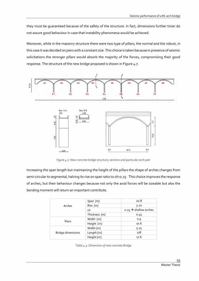
Seismic performance of a RC arch bridge
55 Master Thesis
they must be guaranteed because of the safety of the structure. In fact, dimensions further tinier do
not assure good behaviour in case that instability phenomena would be achieved.
Moreover, while in the masonry structure there were two type of pillars, the normal and the robust, in
this case it was decided on piers with a constant size. This choice is taken because in presence of seismic
solicitations the stronger pillars would absorb the majority of the forces, compromising their good
response. The structure of the new bridge proposed is shown in Figure 4.7.
Figure 4.7: New concrete bridge structure, sections and particular arch-pier
Increasing the span length but maintaining the height of the pillars the shape of arches changes from
semi-circular to segmental, halving its rise on span ratio to r/t=0.25. This choice improves the response
of arches, but their behaviour changes because not only the axial forces will be sizeable but also the
bending moment will return an important contribute.
Arches
Span [m] 20.8
Rise [m] 5.20
r/s 0.25 � shallow arches
Thickness [m] 0.45
Piers Width [m] 0.9
Height [m] 10.6
Bridge dimensions
Width [m] 5.25
Length [m] 178
Height [m] 17.6
Table 4.3: Dimension of new concrete Bridge

From masonry to RC arch bridges: load capability and seismic analysis
56 Master Thesis
The dimension of the elements which constitute the bridge are reported in Table 4.3. It is clear that the
new structure is extremely more slender than the original one, but thanks to the good material it
assures anyway better performances.
Materials and constitutive laws
Modelling with fibre elements results to be strongly favourable, especially if the building is composed
of various materials; like in the case of reinforced concrete. In fact, fibres allow to consider separately
the different constitutive material and behaviour, therefore as consequence it is possible to follow how
each material evolves throughout the analysis process and which one could be reason of collapse or
some type of structural problems.
For this new proposed construction in reinforced concrete, it is chosen to adopt the concrete class
C30/37 and the reinforcing bars of B500A class steel (UNI EN 1992-1-1:2010, §Table 3.1, EN10080).
The mechanical properties of these materials are pointed out in Table 4.4.
Concrete C30/37
Compression strength- fck cylindrical/cubical [MPa] 30/37
Mean compression strength-fcm [MPa] 38
Mean tensile strength-ftm [MPa] 2,9
Modulus of Elasticity- Ec [GPa] 33
Crack strain (‰)-εc1 2.2
Ultimate strain (‰)-εcu 3.5
Reinforcement
B500A
Specific weight- γc [kN/m3] 24
Modulus of Elasticity- Es [GPa] 200
Yield strength- fy [MPa] 500
Strain hardening parameter- μ 1.05
Strain fracture- εu 0.1 Specific weight- γs [kN/m3] 78
Table 4.4: mechanical properties of materials
Figure 4.8: Materials constitutive laws- concrete C30/37 and reinforcement B500A

Seismic performance of a RC arch bridge
57 Master Thesis
The constitutive laws curve of both materials are represented in Figure 4.8.
The dimensions of the sections and their reinforcement dispositions are explained in Appendix B. The
reinforcing steel percentage and configuration, follow the rule given in Eurocode2 for columns in
reinforced concrete.
Numerical model
The computational model is built making use of displacement based DB elements, which were yet
treated in the previous chapter. These elements were chosen for their less heaviness in computational
efforts because of their just two integration points. From the other side, to compensate at this poor
elements integration a good mesh work must be done to do not lose precision in the results.
Each vault is created with 60 elements, each one around 0.45 meter long while the pillars are divided
in 13 elements with a length of around 0.8 meters, except for the extremities which are parts finer and
need more attention in the discretization (Figure 4.9). Both the sections are partitioned in 1000
triangular fibres. Also if this choice entails a harder computational involvement it is adopted to obtain
analysis more accurate especially in the post-elastic phase.
Given that in the proposal of new bridge the spandrel walls are considered to maintain masonry
material, these are not contemplated in the numerical model because for sure they do not confer
stiffness to the bridge. Actually, in case of earthquake the walls are the first element that crack and fail
given the lower resistance of masonry instead concrete. For this reason, it will be necessary to fix the
walls with transversal elements, which do not allow to these elements to fall and create dangerous
situations around the structure.
Figure 4.9: Arches and pier discretization; modelling features.
This basic model is used in all type of leaded analysis, changing the configuration of secondary
elements as spandrel or soil which are implemented as loads or masses depending of the nature of
analysis. For instance in dynamic analysis it is really important the position that a member occupies in

From masonry to RC arch bridges: load capability and seismic analysis
58 Master Thesis
space, because its eccentricity produces secondary effects which change the behaviour of the
structure. In semi-static analysis instead, only the members weight interest as vertical load. In the
following paragraphs the different analysis that are directed are explained in more detail.
In all type of analysis the convergence is achieved with the Newton-Raphson modified algorithm
(explained in the previous chapter) based on displacement and rotation criteria with a tolerance of
10-5 (meter or radiant).
In general, in all the analysis that are performed, some typical performance criteria are fixed that
correspond to a certain level of strain in the materials that constitute the elements. These performance
criteria are notified by the program through assigned colours which allows to follow how the structure
evolves during the analysis. To make to work more clear, eight levels of strains are required as output,
five for the concrete and three for the reinforcement steel and these criteria are kept the same in all
the analysis.
In Table 4.5 the strains fixed for tensile and compression in concrete and for tensile in steel are shown
and the respective colours associated.
Material Name type Strain Colour
Concrete C30/37
ct1 Tensile (ct)
8.846E-05 ct2 0.00026538 cc1
Compression
(cc)
-0.000865 cc2 -0.0015325 cc3 -0.0022
Steel S500 st1
Tensile (st)
0.0025 st2 0.005 st3 0.008
Table 4.5: performance criteria: name, strain value and colour notification related
To better focus these levels of strain they are also represented on the constitutive law curves (Figure
4.10).
Figure 4.10: constitutive laws for concrete and steel: performance criteria points

Seismic performance of a RC arch bridge
59 Master Thesis
This control strategy will be useful in the output interpretation because the chosen points are
important steps of changing for materials and the section, which reaching these levels imply a variation
of behaviour of the whole structure. In fact the response curves will be better explained if the time
steps are also associated to a deformed shape that with performance criteria could show what it is also
occurring in the elements of the model.
4.3 Non-Linear structural Analysis
In the design phase it is fundamental to evaluate how the structure evolves beyond the elastic field,
and which could be its behaviour exposed to different kind of time-history loading curves, as for
instance in a semi-static analysis that carry till collapse, or its horizontal capacity with a push-over or
also finally how it react to an acceleration seismic impulse.
In the following paragraphs these types of analysis are performed, using the fibres approach yet
presented, by the employment of SeismoStruct 7.2 software.
4.3.1 Load-carrying Capability
In order to understand the capacity of the building for vertical loading and the damage process that
induce to the collapse, a non- linear analysis is performed. In the first steps only permanent load are
considered; afterwards the capability is evaluated by the increasing of vertical load set to a quarter span
of the central vault. The quarter span position is chosen because it is the most compromising for the
arches. The live load that is situated on the ground-line is in this way diffused until the arch quote as
nodal incremental forces with an angle of θd=35° (Figure 4.11). In this model the weights of spandrel
walls and of the infill material are arranged as permanent nodal load. The incremental loads for each
node from node14 until node24 are set equal to the unity. So in the first step, for a load factor LF=1 in
the time history analysis the load added to the permanent weight is 11 kN.
Figure 4.11: Nodal incremental load disposition used in the time history analysis

From masonry to RC arch bridges: load capability and seismic analysis
60 Master Thesis
The curve in (Figure 4.12) represents the vertical displacement vs. vertical applied load of the node 24
that results to be most moved. This curve is given only from the incremental results, because for the
self-weight the structure assures the elastic behaviour.
The load-capability of the arch turned from the analysis is correspondent to a LF= 172, well for a force
of ΔF=1887 kN. Related to the masonry bridge that has a capability of about 1220 kN, this new solution
could be a good replacement because it stands in the same order of capability level but presenting a
structure slenderer and materials more advanced.
Figure 4.13 presents the deformed shape of the structure in three important steps of the load process
and the colours explain how the strains evolve in the section of each element, as expressed in Table 4.5.
As possible to understand by the Figure 4.12, the first point (1) of the curve corresponds to the cracking
of concrete in some areas of the arch. The colour of the attendee elements means that in some fibres
of the section the strain reached is equal or higher than ct1= fct/Ec=8.85x10-5.
Figure 4.12: Load-carrying capability curve, node most exposed to direct live load
Following the development of the bridge it is clear that the region most subject to stress is around the
region where incremental loads are directly applied, and the last configuration shows in fact that the
elements reached the maximum strains for steel and concrete materials. After point (2) there is on the
load-capability curve a change of trend, from this point in fact the steel starts to be yielded. In the last
point (3) there is a diffused plasticity. As shown in Figure 4.13 a lot of elements arrived at the crack
strain of concrete but in the most pushed ones, also the last steel tensile and last compression strains
are achieved. In these portions of the arch there an high plasticity level, since that the concrete in some
sections presents the steel in its post-elastic phase and the concrete considerably cracked and
compressed on the opposite boundary.

Seismic performance of a RC arch bridge
61 Master Thesis
In Figure 4.13 (right side) the arch exposed to the live loads is also shown, with its progressive deformed
shapes and performance criteria distinguished for concrete tensile (ct), concrete compression (cc) and
steel tensile (st).
The vertical load capability of the bridge it is not really so high because of the thickness of the arch, but
this is the best compromise obtained searching a structure that could be comparable and a
replacement of the old bridge.
Figure 4.13: Deformed shape (15% scale) and performance criteria for step (1), (2), (3) of Figure 4.12.
This type of incremental analysis was directed for several proposals with different sizes of the
constitutive elements of the viaduct. For instance, structures with robust arches and consequently piers
or with more vaults, are for sure stronger, but are not point of interest in this specific case where the
aim is to find a new solution that works better but without incurs in an over-capacity.

From masonry to RC arch bridges: load capability and seismic analysis
62 Master Thesis
4.3.2 Push-over Analysis
Pushover is a non-linear static analysis where horizontal increasing forces are set to evaluate the
transversal capacity of a structure. This process is a simplifying solution to estimate the possible seismic
response, also if it is more suitable in some specific cases where the structure shown higher regularity.
As reported in paragraph 4.3.3.4.2 of UNI EN 1998-1 the structure analysed with pushover has to own
a certain regularity criterion explained in 4.2.3.2 or 4.3.3.1(8) a)-e) of the same rules.
The method, as previously illustrated, is useful for various purposes: to verify the expected failure
mechanisms and the distribution of damage, to suggest the capacity curve (i.e. base shear vs. control
node displacement) of a building or in other cases to evaluate the performance of an existing structure
(UNI EN 1998-1,2010).
In this static incremental process, the model is firstly exposed to the permanent own-weight loads and
later to a distribution of incremental forces proportional to the masses arrangement of the structure.
Given that the horizontal loads are a ratio of the gravity forces but applied in the transversal direction
the capability curves is expressed in terms of α factor vs. displacements d(mm) of a certain connotative
points of the structure. The α factor is stated as the ratio between the sum of horizontal forces and the
sum of gravity forces:
� = ∑ ³Q∑ ´ ( 4.1
where:
Vb: Base Shear of each support
W: Weight of each elements
It is obvious that the last α factor, corresponding to collapse, expresses the percentage of the self-
weight of the building that this is able to bear in the horizontal direction.
In this type of study is adopted a new model which has masses instead of nodal loads for the infill and
the spandrel walls. The masses are situated in the real barycentre position for the vertical direction,
extruding the nodes from the structural points. For the soil this is a correct position also for the
longitudinal direction. On other hand, for the spandrel walls this choice involves an error, but this
approximation can be considered not really significant seeing that these are lighter than others and
their contribute do not influence so much the global response.

Seismic performance of a RC arch bridge
63 Master Thesis
Figure 4.14: Spandrel wall and infill soil masses disposition on an arch segment
The weights are connected to the structural nodes by means of rigid links; in that way the masses can
interact with the rest of the structural elements, giving a more real contribute in non-static studies. The
disposition just explained is better shown in Figure 4.14.
As previously stated, according to Eurocode 8 (EN 1998-1, 2004), there are different possibilities of
forces distributions in pushover. In this study the mass-proportional load pattern is adopted; in other
words a configuration based on lateral forces proportional to masses.
The horizontal incremental loads are applied to all nodes of arches and piers, as well as to the nodes
where the masses representing fill soil and spandrels are set, and these are augmented under a load
control scheme. This choice derives from the necessity to control the amplitude and regularity of steps.
As convergence criterion it is adopted a displacement/rotation approach with a tolerance of 10-5
(m/rad).
The symmetry of the structure leads to consider the analysis in X and Y direction only in one side given
that the results will be of the same magnitude also in the other part.
The pushover results are shown below for the two directions X and Y; in both analysis the horizontal
assignment of load proportional is the same, but obviously what changes is the direction in which these
forces will push. The different features of the bridge in the two direction will cause a diverse behaviour
in terms of stiffness and collapse mechanism.
Resulting capacity curves are expressed as displacements in X direction of some control nodes on the
horizontal axis, and capacity as function of α factor on the vertical one.
The control nodes displacement is the horizontal contribute of some selected points which are
important to study in the structure behaviour; for instance the top of the crown of the central or
extremity spans or the top of the central pier.

From masonry to RC arch bridges: load capability and seismic analysis
64 Master Thesis
The selected points analysed in the pushover curves are highlighted in Figure 4.15:
Figure 4.15: Selected nodes for pushover capability curves
These displacements are measured, obviously, in the same direction of the incremental applied loads.
Pushover X
The capability curves plotted in Figure 4.16 shows that the last horizontal capacity of the structure in X
direction is around 20% of its self-weight.
Figure 4.16: Pushover curves for Control Nodes (cN) selected in X direction
The five different control points reach different levels of displacements during the process, and it is
clear also that the top of the vaults moves more or less depending on their position related to the
direction of the loads. For example the control node of the last right arch considering a pushover in the
positive direction (cN5) would reach a lower degree of displacement if the analysis would be done in
the negative direction. The same question is valid for the two control nodes of the central spans but
obviously not for the top of the central pier that has for sure the same relative position within the
structure in both directions. It is clear also that the central vaults are allowed to move more because of
their distance from the supports, but the last arch (putting in order with the analysis direction) is the
most stressed one because it bears all the horizontal forces deriving also from the previous arches.
These arguments are clearly illustrated in Figure 4.18, where the deforming process of the bridge is

Seismic performance of a RC arch bridge
65 Master Thesis
shown for some important steps of the analysis. These fundamental stages are explained in the
capability graph of the central span control node (cN1), which will be taken in account also in the
following dynamic analysis as reference point in results comparison.
Figure 4.17: Pushover curve in positive X direction for control Node 1
For these four steps, corresponding to a certain α factor, the deformed shapes is related with the
performance criteria expressed previously in Figure 4.10 and Table 4.5.
From Figure 4.18 it is possible to justify the change of trend of the load-capability curve; in fact it is clear
that each point (1)-(4) on the graph corresponds to the achievement of a particular strain level, shown
with the performance criteria colour. The performance criteria for compression or tension in concrete
and steel are divided for each step, so that the picture could be better readable.
More in detail:
- Step (1) : α= 0.055. The bottom elements of central piers reach the crack tensile strain for concrete,
so the structure leaves the elastic phase and the curve slope starts to vary.
Figure 4.18 (1): deformed shape (15% scale) of step (1) and performance criteria

From masonry to RC arch bridges: load capability and seismic analysis
66 Master Thesis
- Step (2): α= 0.08. This step is shown only to make clear what happens in the middle of steps (1) and
(2). In this interval the cracks continue to grow in arches and in piers too. Some elements start to
reach also a compression strain higher than the elastic one for concrete.
Figure 3.17 (2): deformed shape (15% scale) of step (2) and performance criteria
- Step (3): α=0.17. The tensile and compression strains in concrete continue to be increased and at
this level also steel stars to be not still in its elastic phase and it is yielded, especially this event in the
bottom of central piers change the trend of the capability curve.
Figure 3.17 (3): deformed shape (15% scale) of step (3) and performance criteria
- Step (4) : α= 0.21. In this step that corresponds to the last one, α is the percentage of self weight
that the bridge is able to bear in X direction. At this point the collapse reached with numerical
simulations is related with the maximum compression strain in concrete and a really high tensile
strain in steel in some elements.
Figure 3.17 (4): deformed shape (15% scale) of step (4) and performance criteria
To better understand how the structure evolves during the process, some strain-stress curves of
particular fibres of elements most forced are plotted.
Given that different elements reach the maximum stress-strain values of interest, the most
representative ones are selected and consequently some fibres are studied more in detail. In particular,

Seismic performance of a RC arch bridge
67 Master Thesis
as it is clear also from the performance criteria just shown, two area are mostly interesting: the bottom
of one of the last four piers and the element closed to the support for the last arch (A8).
Figure 4.19 (a): compression (cc) and tension (ct) in concrete fibres
Figure 4.19 (a)-(b) report the strain-stress law for four fibres chosen and belonging to the elements
sections highlighted in the same pictures. It is clear that in the bottom element of the pier the section
reaches high levels of compression and tension; in fact watching to Fibre2 and Fibre4 the curves show
high positive strain in reinforcements and negative in concrete which is in its softening phase.
Figure 3.18 (b): tension (st) in steel fibres
Fibre1 and Fibre3 belonging to the same section (Figure 4.19 (a)-(b)), show how the concrete cracked
continues to increase the strain following completely the steel; in fact their last deformation has the
same value but the stress in concrete is null.

From masonry to RC arch bridges: load capability and seismic analysis
68 Master Thesis
Pushover Y
The distribution of horizontal loads is exactly the same of the previous analysis but in the perpendicular
direction. Also the control nodes are the same five previously chosen.
Figure 4.20: Pushover curves for Control Nodes (cN) selected in X direction
The high stiffness of the piers in Y direction, given by their depth is around five times higher than the
width, carries to results really different from X direction. As shown in Figure 4.20 the last load factor is
around to α~1,this means that the structure, according to computational analysis, can support
approximately its total self-weight applied in Y direction.
Taking into account only one control node and in particular control Node 1 (cN1), its load-capability
curve only for positive X direction is plotted to fix the four steps (1)’-(4)’.
Figure 4.21: (a) Pushover curve in positive Y direction for control Node- (b)Last deformed shape for α=1.0
(b) (a)
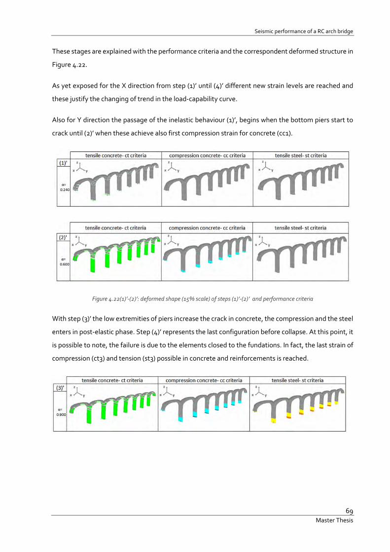
Seismic performance of a RC arch bridge
69 Master Thesis
These stages are explained with the performance criteria and the correspondent deformed structure in
Figure 4.22.
As yet exposed for the X direction from step (1)’ until (4)’ different new strain levels are reached and
these justify the changing of trend in the load-capability curve.
Also for Y direction the passage of the inelastic behaviour (1)’, begins when the bottom piers start to
crack until (2)’ when these achieve also first compression strain for concrete (cc1).
Figure 4.22(1)’-(2)’: deformed shape (15% scale) of steps (1)’-(2)’ and performance criteria
With step (3)’ the low extremities of piers increase the crack in concrete, the compression and the steel
enters in post-elastic phase. Step (4)’ represents the last configuration before collapse. At this point, it
is possible to note, the failure is due to the elements closed to the fundations. In fact, the last strain of
compression (ct3) and tension (st3) possible in concrete and reinforcements is reached.

From masonry to RC arch bridges: load capability and seismic analysis
70 Master Thesis
Figure 3.21 (3)’-(4)’: deformed shape (15% scale) of steps (3)’-(4)’ and performance criteria
For the central pier the lower element is analysed choosing three fibres of which the strain-stress
tendency proves how the structure evolve during the process and why it collapses.
Figure 4.23: strain-stress curves in concrete and steel in three important fibres
Figure 4.23 shows that the collapse is achieved when steel is highly yielded, and concrete is in its
softening branch and it reaches a strain larger than its peak of 0.0022.
In Y direction the structure results to be really stronger than X direction, as predictable due to the depth
of the bridge that confers to piers an high stiffness. The transversal resistance, around five times larger
instead longitudinal direction, imply the decision to consider the following dynamic analysis only for
the weakest side. This choice is further proven by modal analysis performed on the model before the
dynamic ones.

Seismic performance of a RC arch bridge
71 Master Thesis
4.4 Non-linear dynamic analysis
In this paragraph seismic input under accelerograms form are implemented in dynamic time-history
analysis.
For an inelastic system N-DOF, the equation motion is defined by Equation (4.2, where �, } and % are
respectively the mass, the damping and the stiffness matrix �h h�. In the same relation µ��� is the
relative displacement depending on time �; while µ¶ ��� and µ���· are the relative velocity and
acceleration of the system. The term µ·¸��� state the ground acceleration, related to time; therefore
the right factor in the equation stands for the seismic external forces vector (Chopra, 2012):
� ∙ µ· ��� + } ∙ µ¶ ��� + % ∙ µ��� = −� ∙ µ·¸��� (4.2
Thus, it is necessary to have accelerograms available, which, according with rules of UNI EN-1998
(2010) can be historical real data, when possible, or artificial generated in agreement with compatible
elastic response spectra.
Consequently to the creation of accelerograms, the aim is to evaluate the response of the bridge under
earthquake motions which are increased using a scaling factor (SF) from 1 until 10. This method called
IDA (incremental dynamic analysis) is becoming widely adopted and it consists in performing repeated
non-linear dynamic analyses under accelerograms with increasing intensity. The peak ground
acceleration (PGA) obtained by the elastic spectrum is assumed corresponding to a SF=1 and as beyond
shown, it will be increased until 10 because its values is definitely low.
4.4.1 Numerical modal analysis
Eigenvalue analysis are progressed for the evaluation of the structural natural frequencies and mode
shapes. For the present study, this preliminary investigation turn out to be useful for two fundamental
reasons: firstly, to validate the predominant weakness of X direction of the building and consequently
to define the frequency of vibrations of the most important modes. These frequencies and thereby the
periods affect the response of the structure related to the damping in dynamic studies. The first two
mode in X and Y direction are shown in Figure 4.24 and their respective periods (T), frequencies (f),
participating factor (δ) and masses percentage (mx%- my%) provided by fibre elements model are
collected in Table 4.6.

From masonry to RC arch bridges: load capability and seismic analysis
72 Master Thesis
Mode T(sec) f(Hz) δ mx(%) my(%)
mode 1X 0.98 1.02 61.98 81.64 ~0 mode2X 0.18 5.54 25.25 13.24 ~0
mode 1Y 0.30 3.36 53.57 ~0 59.97 mode 2Y 0.25 4.02 13.37 ~0 3.79
Table 4.6: First two modes in X and Y direction and important parameters
Figure 4.24: Deformed shape of the first two modes in X and Y direction.
The bridge conformation, presenting a slender geometry in longitudinal direction instead the
robustness of transversal one, produce a predominance of vibration modes in X direction, especially
the first mode which involve a mass percentage of around 82%. Also the first mode in the Y direction
interests a great percentage of mass (~60%) , but this mode appears for a frequency really higher than
the other one.
In dynamic investigation, it is essential to consider spandrels and fill in terms of mass; therefore, their
representation through point- masses connected by rigid links to the underlying vaults (Figure 4.14) is
necessary. The stiffness of these constitutive elements, on the other hand, is not represented in the
model because these are considered not relevant in the resistance contribution instead reinforced
concrete. Under seismic motion in fact for sure these elements are the first that would crack, therefore
their participation can be not contemplated.
Hence, the main vibration mode allows to decide to study with greater attention the seismic behaviour
in longitudinal direction.

Seismic performance of a RC arch bridge
73 Master Thesis
4.4.2 Seismic Input
Eurocode 8 provides detailed guidelines taking into account the employment of earthquake motion
records. The acceleration curve has to represent a real record, taken from the database kept around
the world, or it can be artificial but following specific features. The latter alternative requires that at
least three independent accelerograms may be adopted in the analysis. Furthermore, this set of
accelerograms, have to present a correspondent elastic spectrum that does not understate the code
spectrum of a maximum of 10% variance (CEN, 2004).
Given that there are not currently records available for the area of Barcelos, for the present study,
artificial earthquake impulses are generated. The Portuguese version of Eurocode 8 specify that two
type of elastic spectrum for the territory of Portugal continental have to be considered, corresponding
to far field and near field earthquake events (CEN, 2010). Moreover, at least three accelerograms must
be adopted.
With reference to Figure 4.25, Barcelos is situated in area 1.6 for action of type-1 and area 2.5 for type-
2. Therefore, taking into account tables NA 3.3-3.4 of the annex of the same Portuguese EN-1998
version, the relative PGA (Peak Ground Acceleration) values are of !¸1 = 0.35 �/�s and !¸s =0.8 �/�s respectively. Experimental survey carried out on the old viaduct, reports that the foundation
soil has a rocky disposition (Costa, et al., 2014), for this reason a type A soil is adopted for the creation
of spectrum with a corresponding soil coefficient ¹¤º` =1. In Table 4.7 are listed the parameters taken
from the norm to create the two types of spectrum.
Figure 4.25: Figure NA.I (CEN, 2010). Seismic zoning for continental Portugal

From masonry to RC arch bridges: load capability and seismic analysis
74 Master Thesis
Type I» [½/¾¿] ?½IC Á Áà ÁB
1 (far field) 0.35 1.0 0.1 0.6 2.0 2 (near filed) 0.8 1.0 0.1 0.25 2.0
Table 4.7: Seismic parameters for Barcelos
Starting from these noted values, the elastic spectrum are delineated by the following relations
assigned in Eurocode 8:
0 ≤ Ä ≤ ÄÅ : ¹c�Ä� = !¸ ∙ ¹ ∙ Æ1 + ''Ç ∙ �È ∙ 2.5 − 1�É ( 4.3
ÄÅ ≤ Ä ≤ Ä{ : ¹c�Ä� = !¸ ∙ ¹ ∙ È ∙ 2.5 ( 4.4
Ä{ ≤ Ä ≤ ÄÊ : ¹c�Ä� = !¸ ∙ ¹ ∙ È ∙ 2.5 ∙ �'Ë' � ( 4.5
ÄÊ ≤ Ä ≤ 4� ∶ ¹c�Ä� = !¸ ∙ ¹ ∙ È ∙ 2.5 ∙ �'Ë'Í' � ( 4.6
where:
¹c�Ä�: Elastic response spectrum.
Ä: Vibration period of a 1DOF correspondent system.
!¸: Design ground acceleration on type A soil.
ÄÅ : Period of beginning of the constant spectral acceleration branch.
Ä{ : Period limit of the constant spectral acceleration branch.
ÄÊ : Period value defining the beginning of the constant displacement response of the spectrum.
¹: Soil factor.
È: Damping correction factor with a reference value È = Î with a viscous damping of 5%.
In terms of displacements, in the same paragraph 3 of the Eurocode 8, is mentioned the equation:
¹Êc�Ä�=¹c�Ä� Æ 'sÏÉs ( 4.7
whit ¹Êc�Ä� elastic response spectrum of displacements.

Seismic performance of a RC arch bridge
75 Master Thesis
The two acceleration spectra present shapes really different with a constant horizontal branch of
different extension and peak acceleration, so that the shape of the near field curve (spectrum-2) results
to be in all cases more conservative. In Figure 4.26 the two elastic spectra are reported, the acceleration
and displacement ones, with the indication of the period of the structure Ts, obtained with modal
analysis before debated. For the generation of artificial earthquake, it is adopted for a simplicity reason,
only spectrum-2 because rather surely, spectrum-1 will involve less intense effects.
Figure 4.26: Elastic accelerogram and displacement spectra-type1 and type2
Spectrum-2 above shown was used to generate three different accelerograms by means of the
software SeismoArtif and SeismoSignal (SeismoSoft) to work on a correction that erases the
imperfections of the curves and checks the quality of the signals. Taking into account the instructions
of Eurocode 8, the duration of seismic impulses must be interrelated with the magnitude and the
principal characteristics of the seismic event and in all cases, it should have at least a duration of 10
seconds for the stationary part. In the present study, it was set to have a duration of 14 seconds with a
rise and fall time of 2 seconds. The three accelerograms get, are expressed in terms of gravity values
and they are chosen from a basket of eight curves looking at the quality of displacements curves too
and corresponding spectra which, as yet remembered, must assure a maximum variation of 10%
from the Eurocode 8 one.

From masonry to RC arch bridges: load capability and seismic analysis
76 Master Thesis
Figure 4.27: three accelerograms generated from spectrum-2, PGA/g=0.0816
From now on, in the present section it will be contemplated ACCELEROGRAM-1 and all its results, while
the information about other two accelerograms, will be attached in the final annex of this essay.
In support of the quality of these artificial time history curves, Figure 4.28 presents the acceleration and
displacement response spectra relative to the first accelerogram (the other two are reported in annex-
A). It is requested in section 3.2.3.1.2 of Eurocode 8, that artificial spectra must be within the 10%
tolerance of the code specified spectra (CEN, 2004). In both spectra, the acceleration and displacement
ones, this criterion is satisfied.
Figure 4.28: Comparison between artificial spectra and Eurocode specified spectra (type2).
In the following paragraphs, the results of mainly the first accelerogram, will be examined except for
the incremental dynamic analysis curve, where the values are referred to the average quantity obtained
from the three results sets.
These accelerograms, although they are created as near field earthquake, own a PGA not really high
so it will be appropriate to increase the Scaling Factor to values rather raised to observe non-linear
behaviour of the structure. In the next paragraph, the seismic simulations are analysed more in detail
and their results are observed and compared with the other analysis outputs, in particular the pushover
ones.

Seismic performance of a RC arch bridge
77 Master Thesis
4.4.3 Analysis setting and parameters
To carry out time history analysis with SeismoStruct, the model implemented is the same yet
illustrated for pushover analysis, with masses representing soil and spandrel walls connected with rigid
link to the principal skeleton of the bridge and DB fibre elements. The material and geometry linger
the same exposed in the previous paragraph 3.2.1 and in particular in Table 4.3 and Table 4.4.
In the definition of the input parameters for this type of non-linear analysis, it is important the choice
of the damping settings.
In SeismoStruct the nonlinear fibre model formulation already include, in non linear dynamic analysis,
implicitly the hysteretic damping in the expressions of inelastic frame elements and in the nonlinear
force-displacement response curve formulation.
However, there is a quantity of non-hysteretic type of damping, that is important to take into account
during dynamic response of structures. This classical damping, which is not directly modelled in the
analysis, is mobilised through other kind of phenomena as for instance could be the friction between
structural and non-structural members or in opened cracks, or the energy dissipation through
foundations. Furthermore, the adoption of even a very low equivalent viscous damping might be very
beneficial in terms of the numerical stability in inelastic dynamic analyses, because its matrix has a
"stabilising" effect in the equations system. Its use is generally suggested, even if small values.
(SeismoSoft, 2014)
The software allows to choose between three different damping formulations: the stiffness or the mass
proportional damping or the Rayleigh damping, that depends on both the properties.
Typically, the Rayleigh dissertation is considered (Chopra, 2012) with a viscous equivalent damping ξ
varying from 1% to 8% depending on the most important structural features, frequencies and mode of
vibration taken into account.
There is a disagreement amongst different scientific authors regarding the use of this parameter, that
represents energy dissipation sources. While some authors recommend the Rayleigh approach, some
others (Priestley and Grant, 2005; Hall, 2006) suggest the use of stiffness-proportional damping only.
In the present work, the stiffness-proportional damping modelling approach is adopted. It is besides
proportional to the tangent stiffness of the structure, given that in nonlinear analysis the stiffness could
considerably change during the process and to fix the initial stiffness might change the real response
of the model.

From masonry to RC arch bridges: load capability and seismic analysis
78 Master Thesis
The damping relation depending on stiffness is expressed from the equation:
} = !1 ∙ % (4.8
where:
}: damping matrix. It is diagonal by virtue of the modal orthogonality properties.
!1: constant parameter [sec]
%: stiffness matrix
With reference to Chopra dynamic theory (Chopra, 2012), the diagonal nth element of stiffness matrix
in the natural vibration motion formulation is expressed as:
,U = ÐUs ∙ gU (4.9
with:
ÑU : natural circular frequency of vibration the nth mode
,U: nth diagonal element of stiffness matrix
gU: nth diagonal element of masses matrix
The generalized damping for the nth mode for a system with stiffness-proportional damping can be
related to the coefficient !1.In fact considering Equation 4.9 in 4.8:
ÒU = !1 ∙ ÐUs ∙ gU (4.10
Given that the damping ratio for the nth mode ÓU can be expressed as:
ÓU = º°s ∙ ÐU (4.11
Depending on the data input of the system it is possible to determine the other factor.
In the present case the damping ratio was fixed equal to ξ=2%; the frequency of the first mode of
vibration Ô1 = 1.02 ÕS (Ð1 = 2 ∙ Ö ∙ Ô = 6.402�!�/�4}�� cause the extracted value of !1:
!1 = s∙× Ø° = '∙×Ï = 0.0062 [�4}] (4.12

Seismic performance of a RC arch bridge
79 Master Thesis
The damping coefficient trend is shown, for the stiffness-proportional approach with the value of the
parameter !1 just evaluated, in Figure 4.29 and it is used in the following time history analysis.
Figure 4.29: Stiffness proportional damping coefficient distribution adopted.
Besides the damping treatment, in time history development the setting of a numerical integration
scheme for the time-stepping method is also significant. This scheme must be availed in order to solve
the system of equations of motion, that seeing the variation of impulses with time and the non-
linearity of the problem would not be possible without the use of a time-stepping method.
The external load of Equation given by the term −� ∙ µ·¸��� = 5���, are a set of discrete values 59 =5��9� defined by a time step ∆� usually constant.
Starting from the instant �9 where the values are known, the response at time �9�1 is obtained by means
of numerical procedures. Generally there are two main possibilities available that consist in explicit and
implicit methods.
Given that in this thesis is used a form of implicit method, only the latter is shortly analysed. In this
method in fact the solution of the system at time �9�1 is directly determined and it turns out to be
stable, instead the other method that does not assure stability for large steps ∆� (Chopra, 2012).
It is adopted in this essay the Hilber-Hughes-Taylor method that is a generalization of the Newmark
method.
The appearance of cracks in concrete, seeing the high post-elasticity behaviour of the analysis,
introduces numerical confusion changing stiffness values suddenly. In these cases, the Hilbert-Hughes-
Taylor integration scheme uses an α-factor used to control the level of numerical dissipation. In
dynamic analysis this α-factor has the role to reduce higher spurious modes' contribution and as
consequence of increase the accuracy of the results as well numerical stability of the analysis.

From masonry to RC arch bridges: load capability and seismic analysis
80 Master Thesis
This scheme uses the same finite difference strategy of the Newmark method but the numerical
integration is controlled by the parameters β and γ.
According to the authors Hilbert an the others (SeismoSoft, 2014), the best solutions, regarding the
accuracy, the analytical stability and numerical damping are found for values of β and γ expressed by
Equations 4.13 and 4.14:
y = 0.25 ∙ �1 − ��s (4.13
Ù = 0.25 − � (4.14
with −1/3 ≤ � ≤ 0. For α= 0 the procedure resumes to the Newmark method, while for −1/3 ≤ � < 0 the scheme is more accurate and stable. The numerical damping depends from this parameter in a
inverse proportional relation; in other words, increasing α the damping decreases.
SeismoStruct default value of the principal factor is � = −0.1.
The time step ∆� previously disputed must be chosen carefully to ensure accuracy. Given that the
accelerograms above reported, are defined with a time phase of 0.01 �4} the analysis are performed
with a ∆� = 0.005 �4}. For a duration of 14 seconds of the earthquake this means a number of 2800
steps. The selected timing ensure a good solution also because referring to the first mode period Ä1 =0.97 �, that involves around the 82% of the structural mass, the ∆� fills a good discretization, about
200 steps for the principal period of vibration.
Finally, in regard to the iterative procedure, the Newton Raphson modified strategy is chosen with
the updating of stiffness matrix, opting for a displacement/rotation convergence criteria with a
tolerance of N ≤ 100v (m) or (rad).
Hence, illustrated all the fundamental aspects pertaining to the dynamic analysis, in the following
subsections the results of the time-history processes carried out, are exposed.
The control point chosen to plot displacement vs. shear base (in the α ratio form) curves is the same
CN1 used in pushover analysis, with the aim to compare also the dynamic response with the pushover
one. The control node selected is an important point of the structure because of its position related to
other structural elements; it is in fact the top node of the central arch, the most distant from each type
of supports and the most exposed to movement as proven in paragraph (4.3.2).
The performance criteria used are exactly the same of previous analysis.

Seismic performance of a RC arch bridge
81 Master Thesis
4.4.4 Time-history analysis
Starting from the original time-history accelerogram values before presented, that corresponds to a
scaling factor SF=1.0, these will be scaled in order to perform an Incremental dynamic analysis and to
assess the seismic performance of the bridge. It is important to point again that in this section only the
results relative to ACCELEROGRAM-1 will be shown, while for ACCELEROGRAM-1 and 2 the output data
will be introduced in the annex-A and their values are also relevant in the IDAs conclusive curve.
Seismic performance 1. PGA1 =0.082 (g)
As earlier stated, the artificial ACCELEROGRAM-1 of type-2 spectrum(near filed), is related to a scale
factor of 1.0 with respect to the Barcelos PGA; therefore, the maximum applied ground acceleration is
!¸1 = 0.08Û.
Figure 4.30 reports the development of the base shear coefficient α (given by ±[/r) related to the
horizontal displacement in its control node. The presented graph corresponds to longitudinal X
direction, given that in this means the accelerogram were applied. The response of control node cN1
for dynamic analysis is shown with pushover curve of the same point. The peak ground acceleration for
this earthquake proves to be really low, so significant values will appear with the increase of the input
seismic forces.
The following graphs of base forces and displacements will maintain from now on the same axes
extension for all the incremental analysis to simplify the comparison between the results. In this specific
case, seeing the lowness of forces is shown in Figure 4.30 (b) also a zoom on the hysteretic curves.
Figure 4.30: (a) hysteretic curves zoom- SF=1.0, (b) hysteretic curves and displacement trend for cN1
(a)
(b)

From masonry to RC arch bridges: load capability and seismic analysis
82 Master Thesis
From this graph, the maximum obtained shear coefficients are 0.038 and 0.036 in the positive and
negative X direction and a maximum displacement value of 6.38 mm.
The deformed shape with performance criteria in terms of strain (Figure 4.31) representing the most
severe damage, turns out that the structure reaches low level of strain, in fact only a few of elements
in arches show to achieve the tensile stress concrete resistance.
Figure 4.31: deformed shape for the most heavy damage for PGA1
From now on the structure will be processed for scaled seismic actions with a scaling factor increased
from between SF=2.0 till to SF=10.0. This procedure was done for each the three artificial
accelerograms generated, so in the extracting phase of the IDA curves the values are obtained as an
average from the three basket results.
Seismic performances for scaled PGA
ACCELEROGRAM-1 is in the present section scaled through growing scaling factors of values variable
from 2.0 till 10.0. As consequence the relative peak ground acceleration changes with the relation:
�£fÜ = ¹Ý ∙ �£f1 (4.15
where s is the related scaling factor value.
The hysteretic curves of the incremental dynamic analysis for the first two increments compared to the
first results are reported in Figure 4.32 , always with the reference of pushover curve capability.
Figure 4.32: (a) Hysteretic curve for 1PGA-2PGA-4PGA vs. pushover; (b) displacement-time trend (cN1)

Seismic performance of a RC arch bridge
83 Master Thesis
The deformed shapes for the most damaging strain configurations relative to 2PGA and 4PGA are
shown in Figure 4.33.
Figure 4.33: Deformed shapes for 2PGA and 4PGA
As possible to note by means of the performance criteria colours, until a level of 4PGA the structure
presents almost an elastic behaviour, only for 4PGA the central pier starts to reach the first step of
tensile strain in concrete.
With the increasing of the scaling factor the hysteretic curves develop increasing the α ratio of base
shear related to the self-weight if the structure, and the displacements values grow too, not with a
linear trend. In particular the negative side, of displacement and of base shear also, manifests higher
values, thus these will be useful in the evaluation of the development of the structure under growing
seismic actions. The evolution of these incremental analysis, are discussed in the following section by
the IDA curves. Shown below, the graph relative to PGA accelerograms actions increased with a SF
from 6 to 10.
Figure 4.34: (a) Hysteretic curve for 6PGA-8PGA-10PGA vs. pushover; (b) displacement-time trend (cN1)

From masonry to RC arch bridges: load capability and seismic analysis
84 Master Thesis
The layout of the corresponding most strained moment in the three processes (Figure 4.35) show
that, with higher values of the peak ground acceleration, the crack tensile strain of concrete in the
bottom elements of the piers starts to be achieved. With a SF of 8 and 10 also the maximum
compression strain in concrete and yield stress in steel, appear in some arches elements.
Figure 4.35: Deformed shapes for 6-8-10 PGA
In the next phase of the work, the results of these incremental dynamic analysis will be considered and
plotted to follow the structure course, and these will be put in relation with the pushover ones.
4.4.5 IDAs results and comparison with Pushover
From the incremental dynamic analysis of the three accelerograms generated, the results are therefore
represented in terms of maximum response under the various scaling factors (Figure 4.36). The
maximum response is identified by maximum displacement of the control node (cN1) for each analysis
and the corresponding (same graph value) base shear, normalized by the self-weight W and expressed
as α factor.
Eurocode 8 specifies that at least three accelerograms should be used for each type of elastic response
spectrum taken into account. For this reason is created a curve which represents the average values of
the three sets of results to compare with pushover curve.
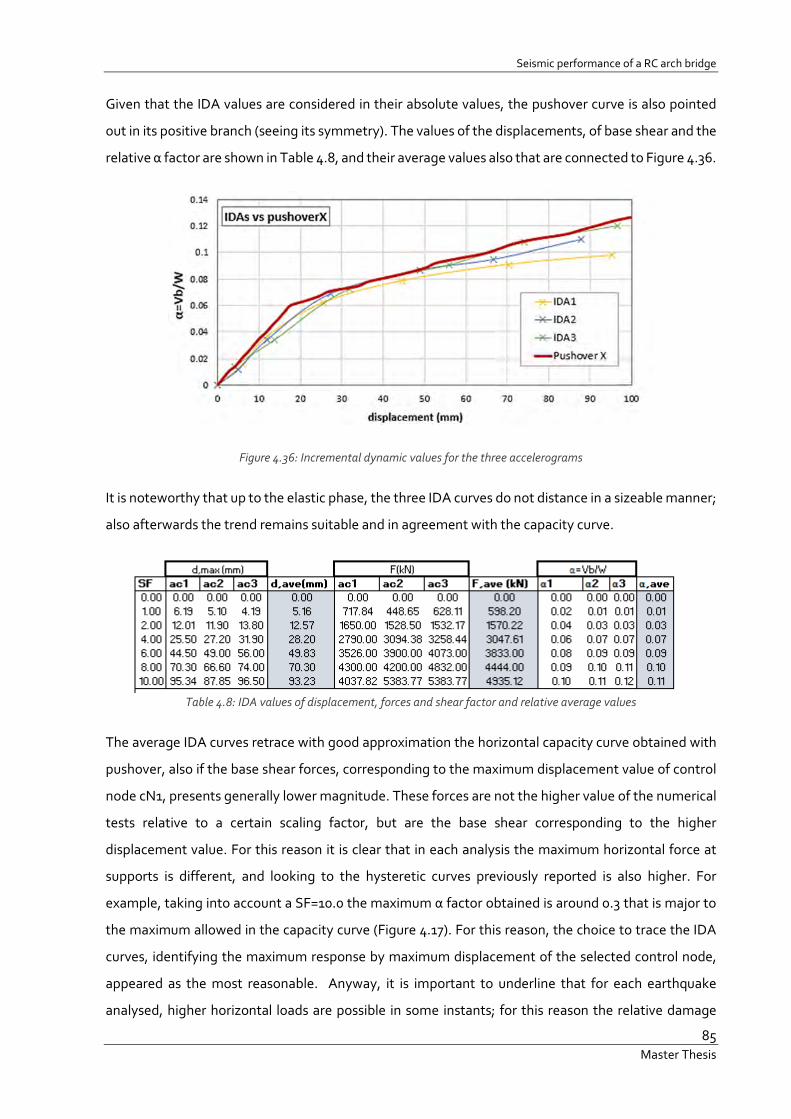
Seismic performance of a RC arch bridge
85 Master Thesis
Given that the IDA values are considered in their absolute values, the pushover curve is also pointed
out in its positive branch (seeing its symmetry). The values of the displacements, of base shear and the
relative α factor are shown in Table 4.8, and their average values also that are connected to Figure 4.36.
Figure 4.36: Incremental dynamic values for the three accelerograms
It is noteworthy that up to the elastic phase, the three IDA curves do not distance in a sizeable manner;
also afterwards the trend remains suitable and in agreement with the capacity curve.
Table 4.8: IDA values of displacement, forces and shear factor and relative average values
The average IDA curves retrace with good approximation the horizontal capacity curve obtained with
pushover, also if the base shear forces, corresponding to the maximum displacement value of control
node cN1, presents generally lower magnitude. These forces are not the higher value of the numerical
tests relative to a certain scaling factor, but are the base shear corresponding to the higher
displacement value. For this reason it is clear that in each analysis the maximum horizontal force at
supports is different, and looking to the hysteretic curves previously reported is also higher. For
example, taking into account a SF=10.0 the maximum α factor obtained is around 0.3 that is major to
the maximum allowed in the capacity curve (Figure 4.17). For this reason, the choice to trace the IDA
curves, identifying the maximum response by maximum displacement of the selected control node,
appeared as the most reasonable. Anyway, it is important to underline that for each earthquake
analysed, higher horizontal loads are possible in some instants; for this reason the relative damage

From masonry to RC arch bridges: load capability and seismic analysis
86 Master Thesis
could be more unsafe than the displacement evaluation choice. Furthermore, the cyclic nature of the
seismic actions, provokes different behaviour from the forecast done with pushover analysis that has a
semi-static way to load the structure. So, the factor of collapse corresponding to load-capability curve,
can be not really representative of the resistance of the bridge in seismic conditions.
Table 4.9 reports the coefficient values corresponding at the same displacement levels of the two
curves, load capability and IDAs put in relation.
Table 4.9: Comparison between pushover and IDA values of displacements, base shear and shear factor.
Figure 4.37: IDA curve for average values of the three accelerograms
The closeness of the two graphs, obtained from different kind of analysis assure a great level of
reliability on the model. Nevertheless, further progresses in the modelling accuracy and numerical
analyses could be implemented in order to render the design more executive. A more accurate
characterization of the geometry of constitutive elements and material properties is compulsory, with
a more fine calibration of the numerical model or a numerical study by means of different approaches
that could support the present study. Given the limited time to lead further works, the treatment of
these tasks should be performed in future studies.

Conclusions and future works
87 Master Thesis
5 Conclusions and future works
5.1 Conclusions
In the present thesis, it is given a possible new solution that could substitute the old masonry viaduct
of Durrães. The work was developed in three fundamental stages.
First of all, the features of the old masonry arch bridges were studied, with its damages and problems
to solve, to continuing to use the bridge at the actual time. Given the possibility to built a new structure
in the area of Barcelos, a new viaduct with the same aspect of the old one was considered. In this sense,
it is important to underline that, starting from the original multi-span arches scheme of Durrães
viaduct, a new proposal that keeps the same aspect but involves more current materials was suggested.
The new bridge, that was conceived in reinforced concrete, was chosen from a set of possibilities, in
order to conserve the same grade of resistance magnitude of the previous one. This decision was taken
because the bridge must preserve the same functions of before and it is important to not over-design
the capacity of the new structure. Once that the possible new bridge features were fixed, the study of
the latter in terms of non-linear response was taken into account. Inelastic analysis of the numerical
model, were simulated by means of fibre approach and in particular using SeismoStuct software. The
non-linear analysis expanded were vertical time-history load, pushover in both transversal direction of
the bridge and dynamic analysis. The last two non-linear methods were used to assess the seismic
behaviour of the structure: static pushover and time-history dynamic analyses. In the first case, mass-
proportional loading configuration was employed to obtain the two capacity curves in X and Y
direction. From this type of analysis and from the eigenvalues one, the bridge is clearly more weak in
its longitudinal direction; for this reason the following dynamic incremental analysis are considered
only in X direction. Regarding the dynamic method, three artificial accelerograms were generated and
the building was subjected to these seismic impulses which present the same peak ground
acceleration.
The responses of all the previous analyses, were given in terms of capacity curves and damage pattern
of the structure presented by deformed shapes and performance strain criteria.
Based on the steps of the work, it is possible to deduce the following conclusions:
Considering the non-linear analysis for vertical loads:
The vertical capacity of the structure was assessed, loading the middle arch with increasing forces in
vertical direction in an area nearby the quarter span. This kind of analysis was used to choose also the
best compromise between different possibilities. Maintaining the previous order of resistance the new

From masonry to RC arch bridges: load capability and seismic analysis
88 Master Thesis
bridge bears a load of around 1900 kN localized in this particular point of the arch. The mechanism of
failure in this specific case corresponds to the localized failure of the arch, which presents four plasticity
areas at the moment of collapse.
Considering the pushover method for X and Y direction:
The last shear factor in X , expressed as the ratio between the base shear at support (in the direction
considered) , is around α=0.2. This means that the structure in its longitudinal direction is able to bear
until a percentage of 20% of its self-weight. Whereas in Y direction the maximum load factor reached
is α=1, so the total of its self-weight. It is easy gather that in Y direction the stiffness of the bridge is
higher, and from this point the seismic analysis are considered only in X direction. The failure in both
directions occurs in the bottom of the piers that are strongly partialised and the steel is yielded. It is
obvious that in Y direction the piers own a size five times higher than in X direction, so the reserves are
more. In this pushover analysis the load configuration is considered proportional to masses only, and
the first mode of vibration is not taken into account. This aspect is a superficial assumption, because a
deeper examination on the kind of response given by different load distribution should be done to
make the interpretation more reliable. In the present work, for the shortage of time available, and as
introductory study before the executive design, this type of analysis has been considered satisfying.
Considering the non-linear dynamic method:
The previous study on modal behaviour confirmed that the seismic behaviour of the bridge is governed
by its longitudinal direction, because the lowest values of shear factor and maximum displacements of
the control node were estimated. The first mode vibration period T1=0.97 s is out from the flat part of
the elastic spectrum curve. This mode that involve about 72% of the structural mass falls out from the
flat part of the elastic spectrum. This means that the bridge in X direction has a good flexibility and the
seismic loads effecting are not in their maximum value. In this sense, the first mode of the Y direction
that presents a period of 0.27 sec. could be exposed to higher forces, given also to its bigger stiffness.
Anyway, the small value of the peak ground acceleration and the big amount of the mass contributing
to the first mode in X direction, make the longitudinal direction the most risky of the two. The
Portuguese rules request two type of seismic analysis, referred to far and near field elastic spectrum.
In case of Barcelos, the near field spectrum stands always above the far field curve; for this reason only
the second type spectrum is analysed because it is considered more demanding. The three
accelerograms artificially generated with SeismoArtif present a PGA=0.08g that is a low value for the
structure. To see inelastic behaviour in fact the structure must be subjected to scaled accelerograms;
in this way the incremental dynamic analysis results can be collected in a curve presenting maximum

Conclusions and future works
89 Master Thesis
displacements and relative base shear, which is compared with the load-capability curve of pushover.
The two curves are in a good agreement with a maximum variation of the 10%.
5.2 Future development opportunities
The presented study gives an opportunity of new solution in substitution to the old masonry viaduct of
Durrães, situated in Barcelos (Braga, Portugal). The old bridge that presents various damages needs a
strong refurbishment or eventually a modern bridge, with new materials, that could maintain the
original features but better services. In future developments of the work, the solution proposed could
be examined in depth under various points of view. Firstly before that the design can become
executive, a optimization of the geometry is necessary. Consequently also a numerical modelling
improvement can be done, taking into account the contribution of non-structural masses in a more
accurate way and trying to compare the formulation with fibres with other type of modelling
techniques. Furthermore, pushover analysis with other kind of load dispositions should be proposed
and compared also with seismic time-history studies. The accelerograms artificially generated could
be replaced by real time history curves, taken from historical events and presenting the same duration
and the same PGA. In the present work, this research would use too much time than the availability
allowed. Finally, for sure, a good study of seismic behaviour also in transversal and vertical direction
could be useful to totally understand the structural response of the bridge. In that way the new bridge
project can be optimized and can represents a great replace of the old viaduct and a good and safe
structure for modern times.

90 Master Thesis - Erasmus +

References
91 Master Thesis
References
CEN Eurocode 8: Design of structures for earthquake resistance - Part 1: General rules, seismic actions
and rules for buildings [Conference]. - 2004. - Vol. 3.
CEN Eurocòdigo 8: Projecto de estructuras para resistencia aos sismos-versao portoguesa
[Conference]. - 2010. - Vol. 3.
Chopra Anil K. Dinamics of structures- Theory and Applications to Earthquake Engineering [Book]. -
[s.l.] : Prentice Hall, 2012.
Costa C. and al. et AVALIAÇÃO EXPERIMENTAL E NUMÉRICA DOS PARÂMETROS MODAIS DA
PONTE FERROVIÁRIA DE DURRÃES [Journal]. - [s.l.] : JPEE-5as Jornadas Portuguesas de Engenharia
de Estruturas, 2014.
da Cruz Morais Maria José Pontes em Arco de Alvenaria - Estudo de um Caso Prático [Book Section] /
book auth. Escola Instituto Politécnico de Viseu. - 2012.
Da Porto F. and Longo F. A brief overview of nonlinear analysis of R.C structures. - [s.l.] : Univerity of
Padova, 2013.
De Felice G. Assessment of the load-carrying capacity of multi-span masonry arch bridges using fibre
beam elements [Journal]. - [s.l.] : Elsevier, Engineering Structures, 2009. - 8 : Vol. 31.
De Santis S. Modelling brickwork elements through fiber beams [Book Section] // Load-carrying
capability and seismic assessment of masonry bridges. - Roma : University Roma Tre, 2011.
De Santis Stefano and De Felice Gianmarco Overwiev of a railway masonry bridge with a safety factor
estimate [Journal]. - [s.l.] : International journal of Architectural Heritage, 2014.
De Santis Stefano Load-carrying capability and seismic assessment of masonry bridges [Online]. -
2011. - https://www.sendspace.com/file/7sjjuv.
De Santis Stefano Load-carrying capability of masonry bridges [Book Section] // Load-carrying
capability and seismic assessment of masonry bridges. - Roma(Italy) : [s.n.], 2011.
De Santis Stefano Safety assessment of different typologies of Italian large-span rail bridges [Book
Section] // Load-carrying capability and seismic assessment of masonry bridges. - Roma : [s.n.], 2011.

From masonry to RC arch bridges: load capability and seismic analysis
92 Master Thesis
Gilbert M Limit analysis applied to masonry arch bridges : state-of-the-art and recent developments
[Rivista]. - University of Sheffield, Department of Civil & Structural Engineering, Sheffield, UK. : ARCH
'07-5th International Conference on Arch Bridges, 2007.
Gilbert M. Limit analysis applied to masonry arch bridges : state-of-the-art and recent developments
[Journal]. - University of Sheffield, Department of Civil & Structural Engineering, Sheffield, UK. : [s.n.],
2007. - Vol. 5th International Conference on Arch Bridges.
Jackson Donald C. Great American Bridges and Dams [Book]. - [s.l.] : John Wiley & Sons, 1988.
Lake Havasu City, AZ : London Bridge in Lake Havasu City [Online] // city-data.com. - 1 may 2004. - 29
janaury 2015. - http://www.city-data.com/picfiles/pic1141.php.
Lourenço P.B,, Oliveira D. and Portela A. Arch'07-5th international Confernce of Arch Bridges [Book
Section]. - Madeir, Portugal : Multicomp.Lda, 2007.
Marefat Mohammad S., Ghahremani-Gargary Esmaeel and Ataei Shervan Load test of a plain
concrete arch railway bridge of 20-m span [Journal]. - [s.l.] : Elsevier, 2004. - Vol. 18.
Oliveira D. and Moreira V.N. Avaliação de Segurança de Pontes Existentes . Aplicação ao Viaduto de
Durrães. - Escola de engenheria : Universidade do Minho, 2014.
Oliveira Daniel V., Lourenço Paulo B. and Lemos Clàudia Geometric issues and ultimate load
capacity of masonry arch bridges from the northwest Iberian Peninsula [Journal]. - [s.l.] : Elsevier,
2010. - Vol. 32.
Professor C. Melbourne, Gilbert M and Wagstaff M The collapse behaviour of muItispan brickwork
arch bridges [Journal]. - University of Salford,University of Sheffield,Bolton Institute : The Structural
Engineer, 1997. - 17 : Vol. 75.
Proske D. and Gelder P. Damages on Historical Arch Bridges [Book Section] // Safety of Historical
Stone Arch Bridges. - [s.l.] : Springer, 2009.
Proske Dirk and Van Gelder Pieter 3.Computation of Historical Arch Bridges [Book Section] // Safety
of Historical Stone Arch Bridges. - [s.l.] : Springer, 2009.
Proske Dirk and Van Gelder Pieter Safety of Historical Stone Arch Bridges [Book]. - [s.l.] : Springer,
2009.

References
93 Master Thesis
SeismoSoft Seismostruct User Manual [Book]. - Pavia : [s.n.], 2014.
SeismoStruct User Manual [Book]. - for version 7.
Solazzo Francesco Ponti e Viadotti Ferroviari [Online] // ingegneria solazzo. - 02 09 2015. -
http://www.ingegneriasolazzo.it/Articoli/2014/10.PONTI%20E%20VIADOTTI%20FERROVIARI.pdf.
Spacone LA, Filipou CE berkley [Online]. - August 1992. -
http://www.ce.berkeley.edu/~filippou/Research/P.
various London Bridge (Lake Havasu City) [Online] // Wikipedia. - 0ctober 2014. - january 2015. -
http://en.wikipedia.org/wiki/London_Bridge_(Lake_Havasu_City).
Viesi Fausto Confronto tra modellazione a plasticità diffusa e concetrata [Book]. - Bologna : [s.n.],
2008.
Zanardo G. [et al.] Performance Evaluation of Short Span Reinforced Concrete Arch Bridges
[Journal]. - [s.l.] : JOURNAL OF BRIDGE ENGINEERING-ASCE, 2004.
Zienkiewicz O.C. and Taylor R.L. The Finite element Method [Book]. - [s.l.] : BH, 2000.

From masonry to RC arch bridges: load capability and seismic analysis
94 Master Thesis

Appendix A
95 Master Thesis
Appendix A
In the present appendix there are reported the results of the three dynamic incremental analysis in
terms of hysteretic curves, time-displacement curve and deformed shape with strain performance
criteria.

From masonry to RC arch bridges: load capability and seismic analysis
96 Master Thesis
ACCELEROGRAM-1
1PGA
2PGA
4PGA

Appendix A
97 Master Thesis
6PGA
8PGA
10PGA

From masonry to RC arch bridges: load capability and seismic analysis
98 Master Thesis
ACCELEROGRAM-2
1PGA
2PGA
4PGA

Appendix A
99 Master Thesis
6PGA
8PGA
10PGA

From masonry to RC arch bridges: load capability and seismic analysis
100 Master Thesis
ACCELEROGRAM-2
1PGA
2PGA
4PGA

Appendix A
101 Master Thesis
6PGA
8PGA
10PGA

From masonry to RC arch bridges: load capability and seismic analysis
102 Master Thesis

Appendix B
103 Master Thesis
Appendix B
In this Appendix more details regarding the sections of the arches and piers are reported, just to show
the disposition of reinforcements. The values of the reinforcement configuration and quantity are
exposed in the table below. The values referred to ‘w’ mean the reinforcements of the width, the ones
referred to ‘t’ mean the thickness.
Pier-section

From masonry to RC arch bridges: load capability and seismic analysis
104 Master Thesis
Arch-section

105 Master Thesis

From masonry to RC arch bridges: load capability and seismic analysis
106 Master Thesis