universitÉ nice - sophia antipolis laboratoire d
TRANSCRIPT
UNIVERSITÉ NICE - SOPHIA ANTIPOLIS
Laboratoire d’Electronique, Antennes etTélécommunications (LEAT)
Ecole Doctorale STIC, Information and Communication Sciences &
Technologies
ULM UNIVERSITY
Institute of Microwave Techniques (MWT)Faculty of Engineering and Computer Science
P H D T H E S I S
Armin Zeitler
Investigation of mm-Wave Imaging andRadar Systems
defended on January 11, 2013
Supervisors LEAT: Prof. Dr. Claire Migliaccio
Prof. Dr. Jean-Yves Dauvignac
Supervisor MWT: Prof. Dr.-Ing. Wolfgang Menzel
Jury:
Reviewers: MCF (HDR) Dr. Amélie Litman, Université Aix-MarseilleProf. Dr. Alexander Yarovoy, Delft University of TechnologyProf. Dr.-Ing. Wolfgang Menzel, University of Ulm
Head of Jury: Prof. Dr.-Ing. Hermann Schumacher, University of Ulm
Examinators: Prof. Dr. Jean-Yves Dauvignac, Université Nice-Sophia AntipolisMCF Dr. Ioannis Aliferis, Université Nice-Sophia AntipolisProf. Dr. Claire Migliaccio, Université Nice-Sophia Antipolis
Dean University of Ulm: Prof. Dr.-Ing. Klaus Dietmayer


Investigation of mm-Wave Imaging and Radar Systems by Armin Zeitler islicensed under a
Creative Commons Attribution-NonCommercial-NoDerivs 3.0 Unported License.


Acknowledgment
This thesis has resulted from a cooperation between the University of Nice - SophiaAntipolis and the University of Ulm.
First of all, I thank my supervisor and mentor Prof. Dr. Claire Migliaccio:she guided me through my diploma thesis and found me a possibility to stay asresearch engineer for nine month at LEAT to present a valuable topic which hasbeen financed by a French state scholarship. She supervised my the last five yearstowards the Ph.D. and has always been here to discuss technical as well as personalconcerns. Furthermore, I highly acknowledge Prof. Dr. Jean-Yves Dauvignac,actual director of LEAT, for the supervision and support as well as for enabling meto work in his laboratory. At this point I also thank Dr. Pichot, former directorof LEAT, for the numerous delightful discussions. Additionally, I am grateful toDr. Ioannis Aliferis for providing me the spirit for valuable software engineeringand its importance. Special thanks to Laurent Brochier and Franck Perret for theassistance in installing the measurement system.
I would like to express my very sincere and deep thanks to Prof. Dr.-Ing.Wolfgang Menzel who set the basis for this work as he accepted an external diplomathesis at LEAT in 2008. This would not be possible without the motivation ofthis idea of Dr.-Ing. Peter Feil and I owe him my thanks. Many thanks belongto Dr.-Ing. Frank Bögelsack who provided me with assistance in all questionsconcerning documentation and presentation of results.
For reviewing this manuscript and for their useful remarks and suggestionsthat helped to improve this manuscript I thank Dr. Amélie Litman and Prof. Dr.Alexander Yarovoy. I express my gratitude to Prof. Dr.-Ing. Hermann Schumacherfor being the president of the jury.
I am deeply grateful to all my colleagues at LEAT for the great moments weshared together within but also beside the laboratory.
Also, I thank Savina, without her support, this work would not be possible tobe accomplished. Finally, I would also like to thank my parents for their sacrifice,encouragement and support throughout my studies.
Munich, March 2013Armin Zeitler


Contents
1 Introduction 1
2 Electromagnetic Modeling 5
2.1 Introduction of the Problem . . . . . . . . . . . . . . . . . . . . . . . 52.2 Electromagnetic Modeling of the Direct Problem . . . . . . . . . . . 9
2.2.1 Numerical Solution . . . . . . . . . . . . . . . . . . . . . . . . 92.2.2 Analytic Solution . . . . . . . . . . . . . . . . . . . . . . . . . 162.2.3 Description of the Means of Simulation . . . . . . . . . . . . . 17
2.3 Qualitative Imaging - Localization and Shaping . . . . . . . . . . . . 252.3.1 Back-propagation - Monochromatic Approach . . . . . . . . . 252.3.2 Back-propagation - Multifrequency Approach . . . . . . . . . 28
2.4 Quantitative Imaging - Reconstruction of the Complex Permittivity . 302.4.1 Description of the Inversion Algorithm . . . . . . . . . . . . . 302.4.2 Quantitative Imaging Performance for Metallic Objects . . . 312.4.3 Quantitative Imaging Results . . . . . . . . . . . . . . . . . . 31
3 Scattered Field Measurement System for Imaging with mm-Waves 35
3.1 Comparison of Existing Systems . . . . . . . . . . . . . . . . . . . . 353.1.1 Two Dimensional Scattered Field Measurement Facilities . . . 353.1.2 Measurement Systems Providing Three Dimensional Results . 363.1.3 Compact Range Antenna Facilities . . . . . . . . . . . . . . . 37
3.2 Description of the Measurement System . . . . . . . . . . . . . . . . 383.2.1 Introduction of Objectives . . . . . . . . . . . . . . . . . . . . 383.2.2 Description of Mechanical Modifications . . . . . . . . . . . . 383.2.3 Millimeter-Wave Antenna Measurement System . . . . . . . . 423.2.4 Investigated Measurement Area . . . . . . . . . . . . . . . . . 42
3.3 Measurement Results . . . . . . . . . . . . . . . . . . . . . . . . . . . 443.3.1 Measurement Parameters . . . . . . . . . . . . . . . . . . . . 443.3.2 First Measurement Results . . . . . . . . . . . . . . . . . . . 44
3.4 Analysis and Error Correction . . . . . . . . . . . . . . . . . . . . . . 583.4.1 Characterization of Dielectric Targets . . . . . . . . . . . . . 583.4.2 Precision of Setup Installation - Correction of Mechanical Errors 603.4.3 Match Experimental Setup with Simulation - Complex Nor-
malization . . . . . . . . . . . . . . . . . . . . . . . . . . . . . 663.4.4 Noise Sources - Filtering . . . . . . . . . . . . . . . . . . . . . 67
3.5 Results over W-band and Discussion . . . . . . . . . . . . . . . . . . 793.5.1 Calibrated and Normalized Measured Scattered Fields . . . . 793.5.2 Overall Calibration Performance and Measurement Error . . 873.5.3 Mechanical Precision Versus Measurement Error . . . . . . . 87
3.6 Conclusion . . . . . . . . . . . . . . . . . . . . . . . . . . . . . . . . . 88

vi Contents
4 Qualitative and Quantitative Reconstruction 91
4.1 Qualitative Imaging . . . . . . . . . . . . . . . . . . . . . . . . . . . 914.1.1 Localization of Targets . . . . . . . . . . . . . . . . . . . . . . 914.1.2 Reconstruction . . . . . . . . . . . . . . . . . . . . . . . . . . 94
4.2 Quantitative Imaging . . . . . . . . . . . . . . . . . . . . . . . . . . . 984.2.1 Estimation of the Domain’s Size . . . . . . . . . . . . . . . . 994.2.2 Expected Complex Permittivity Values . . . . . . . . . . . . . 1014.2.3 Inversion Results . . . . . . . . . . . . . . . . . . . . . . . . . 101
4.3 Conclusion . . . . . . . . . . . . . . . . . . . . . . . . . . . . . . . . . 106
5 FMCW-Radar Measurements 107
5.1 Introduction of Application . . . . . . . . . . . . . . . . . . . . . . . 1075.2 Theoretical Results - Simulation . . . . . . . . . . . . . . . . . . . . 1095.3 Ideal Setup with Network Analyzer . . . . . . . . . . . . . . . . . . . 112
5.3.1 Scene with Vertical Cylinders . . . . . . . . . . . . . . . . . . 1125.3.2 Detection of Foreign Object Debris . . . . . . . . . . . . . . . 116
5.4 FMCW-Radar System . . . . . . . . . . . . . . . . . . . . . . . . . . 1205.4.1 Sensor Overview and Signal Processing . . . . . . . . . . . . . 1205.4.2 Measurement Results . . . . . . . . . . . . . . . . . . . . . . . 122
5.5 Conclusion . . . . . . . . . . . . . . . . . . . . . . . . . . . . . . . . . 127
6 Conclusion and Outlook 129
6.1 Conclusion . . . . . . . . . . . . . . . . . . . . . . . . . . . . . . . . . 1296.2 Outlook . . . . . . . . . . . . . . . . . . . . . . . . . . . . . . . . . . 129
7 Resume in German and French 131
7.1 Zusammenfassung und Ausblick auf Deutsch . . . . . . . . . . . . . . 1317.2 Résumé en français . . . . . . . . . . . . . . . . . . . . . . . . . . . . 133
A Approach of the Integration of the Green’s Function 137
A.1 Self Element Case, n = m, Diagonal Matrix Elements . . . . . . . . . 138A.2 General Case, n 6= m, Non-diagonal Matrix Elements . . . . . . . . . 140
B Approach for the Integration over a Squared Disc with an Optimal
Circular Disc 143
B.1 Demonstration . . . . . . . . . . . . . . . . . . . . . . . . . . . . . . 143B.2 Numerical Integration . . . . . . . . . . . . . . . . . . . . . . . . . . 146
B.2.1 Approximate Integration . . . . . . . . . . . . . . . . . . . . . 146B.2.2 Approximate Double Integration . . . . . . . . . . . . . . . . 147
B.3 Chosen Approach versus Numerical Integration . . . . . . . . . . . . 147B.3.1 Wavelength in the Order of Meters . . . . . . . . . . . . . . . 147B.3.2 Wavelength in the Order of Millimeters . . . . . . . . . . . . 149
C Additional Scattered Field Measurements 151

Contents vii
Bibliography 167
Publications of the Author 179
Curriculum Vitae 181


List of Symbols and Abbreviations
Well known operators and functions are not stated here. The page numbers pointto the first appearance of a symbol or abbreviation.
Symbols
ρ Charge. . . . . . . . . . . . . . . . . . . . . . . . . . . . . . . . . . . . . . . . . . . . . . . . . . . . 6J Current . . . . . . . . . . . . . . . . . . . . . . . . . . . . . . . . . . . . . . . . . . . . . . . . . . . 6e jωt Time dependency convention . . . . . . . . . . . . . . . . . . . . . . . . . . . . . . 6r Vector to point of observation in space . . . . . . . . . . . . . . . . . . . . 7E(r) Total field observed at r . . . . . . . . . . . . . . . . . . . . . . . . . . . . . . . . . . 7E(i)(r) Incident field observed at r . . . . . . . . . . . . . . . . . . . . . . . . . . . . . . . .8E(s)(r) Scattered field observed at r . . . . . . . . . . . . . . . . . . . . . . . . . . . . . . 8∆φ Angle step size . . . . . . . . . . . . . . . . . . . . . . . . . . . . . . . . . . . . . . . . . . . 21λ0 Free-space wavelength. . . . . . . . . . . . . . . . . . . . . . . . . . . . . . . . . . . .21
A(s)z Amplitude of scattered field in z-direction . . . . . . . . . . . . . . . . 62
A(t)z Amplitude of total field in z-direction . . . . . . . . . . . . . . . . . . . . 62
A(i)z Amplitude of incident field in z-direction . . . . . . . . . . . . . . . . . 62
Φ(s) Phase of scattered field . . . . . . . . . . . . . . . . . . . . . . . . . . . . . . . . . . 62Φ(t) Phase of total field . . . . . . . . . . . . . . . . . . . . . . . . . . . . . . . . . . . . . . . 62Φ(i) Phase of incident field. . . . . . . . . . . . . . . . . . . . . . . . . . . . . . . . . . . .62E
(s)cal. Calibrated measured scattered field . . . . . . . . . . . . . . . . . . . . . . 66
γ Complex normalization factor . . . . . . . . . . . . . . . . . . . . . . . . . . . . 66
E(s)cal.,norm. Measured scattered field calibrated and normalized . . . . . . . 66
e Measurement error . . . . . . . . . . . . . . . . . . . . . . . . . . . . . . . . . . . . . . . 67E
(s)exact Exact scattered field . . . . . . . . . . . . . . . . . . . . . . . . . . . . . . . . . . . . . 67

x List of Symbols and Abbreviations
Abbreviations
FOD Foreign Object Debris . . . . . . . . . . . . . . . . . . . . . . . . . . . . . . . . . . . . . 1RCS Radar Cross Section . . . . . . . . . . . . . . . . . . . . . . . . . . . . . . . . . . . . . . 2TE Transverse Electric . . . . . . . . . . . . . . . . . . . . . . . . . . . . . . . . . . . . . . . . 5TM Transverse Magnetic . . . . . . . . . . . . . . . . . . . . . . . . . . . . . . . . . . . . . . 5EFIE Electric Field Integral Equations . . . . . . . . . . . . . . . . . . . . . . . . . . 9MoM Method of Moments . . . . . . . . . . . . . . . . . . . . . . . . . . . . . . . . . . . . . 11PEC Perfect Electric Conductor . . . . . . . . . . . . . . . . . . . . . . . . . . . . . . . 20SNR Signal-to-Noise Ratio . . . . . . . . . . . . . . . . . . . . . . . . . . . . . . . . . . . . 23FMCW Frequency-Modulated Continuous Wave . . . . . . . . . . . . . . . . . . 28SFCW Stepped Frequency Continuous Wave. . . . . . . . . . . . . . . . . . . . .28TUT Target Under Test . . . . . . . . . . . . . . . . . . . . . . . . . . . . . . . . . . . . . . . 30AWGN Additive White Gaussian Noise . . . . . . . . . . . . . . . . . . . . . . . . . . 31SFMS Scattered Field Measurement System. . . . . . . . . . . . . . . . . . . . .35CATR Compact Antenna Test Range . . . . . . . . . . . . . . . . . . . . . . . . . . . 35CAF Complex Antenna Factor . . . . . . . . . . . . . . . . . . . . . . . . . . . . . . . . 45PMMA Polymethyl Methacrylate . . . . . . . . . . . . . . . . . . . . . . . . . . . . . . . . 58CCD Charge-Coupled Device . . . . . . . . . . . . . . . . . . . . . . . . . . . . . . . . . 107LIDAR Light Detection and Ranging . . . . . . . . . . . . . . . . . . . . . . . . . . . 107LADAR Laser Detection and Ranging . . . . . . . . . . . . . . . . . . . . . . . . . . . 107MMIC Monolithic Microwave Integrated Circuit . . . . . . . . . . . . . . . . 107FAA Federal Aviation Administration . . . . . . . . . . . . . . . . . . . . . . . . 108PLL Phase Locked Loop . . . . . . . . . . . . . . . . . . . . . . . . . . . . . . . . . . . . . 120VCO Voltage-Controlled Oscillator . . . . . . . . . . . . . . . . . . . . . . . . . . . 120LO Local Oscillator . . . . . . . . . . . . . . . . . . . . . . . . . . . . . . . . . . . . . . . . . 120DDS Direct Digital Synthesis . . . . . . . . . . . . . . . . . . . . . . . . . . . . . . . . . 121ADC Analogue Digital Conversion . . . . . . . . . . . . . . . . . . . . . . . . . . . . 121
Chapter 1
Introduction
In the last decade, microwave and millimeter-wave systems have gained importancein civil and security applications. Due to an increasing maturity and availability ofcircuits and components, these systems are getting more compact while being lessexpensive. Millimeter-wave systems—less affected by atmospheric conditions thanthose working in the infrared and visible spectrum—are currently being developedin a wide range of areas: their development is mainly driven by automotive appli-cations at 24GHz [1, 2] and 77GHz [3]. Niche applications take advantage of thissuccess, like power line detection at 77GHz and 94GHz [4–7] and Foreign ObjectDebris (FOD) detection at 77GHz [8]. The choice for this frequencies is basedon the short wavelength, providing a high resolution by itself, and the feasibilityof directive antenna systems within compact platforms. All these applicationscan be classified under the terms of qualitative imaging and detection of objectsand obstacles [1, 2, 4–13]. One is able to detect and localize objects but in orderto classify them precisely these systems are pushed to identification nowadaysthat means an extension to more adequate imaging is needed. On one hand, thisrequires the improvement of the radar module itself to get a three dimensionalimage. On the other hand, the targets have to be reconstructed with qualitativeand/or quantitative imaging algorithms.
Quantitative imaging has been conducted at lower frequencies [14–20] usingcomputationally intensive inverse problem algorithms. Due to the ill-posed charac-ter of the inverse problem, these algorithms are, in general, very sensitive to noise:the key to their successful application to experimental data [21–25] is the precisionof the measurement system. Only a few research teams investigate in imaging inthe W-band or higher frequencies, where real-time back-propagation algorithmshave been successfully applied [26–31].
The requirements for the presented work are developed based on formerresearch activities of the two laboratories where this work is effected. In the past,measurements of radiation patterns of antennas in the W-band (75 - 110GHz) havebeen successfully provided at LEAT [32], [113–118] in a laboratory environment,the anechoic chamber, on one hand. On the other hand, radar measurementshave been done [33], [119, 120] in collaboration with the MWT [4, 8], [121].Additionally, quantitative imaging algorithms have been developed at LEAT andsuccessfully applied to measured data provided by academic partners, so far atlower frequencies [17,19,34,35]. Therefore, this manuscript should demonstrate the

2 Chapter 1. Introduction
combination of these three mentioned competences: one would provide controlledmeasurements of scattered fields in the W-band, which can be used for quantitativeimaging in order to develop further algorithms at this frequency band of interest.Furthermore, a first proposal should be developed in order to obtain “in-field”measurements with a radar system to get closer to applications of interest. To ourbest knowledge, there is no experimental system associated with a comparison ofthe scattered field of targets, in the amplitude and in the phase, with theoreticalresults in the W-band. In this manuscript such a system is presented, designed toprovide scattered field data to quantitative reconstruction algorithms.
For qualitative imaging purposes, one can directly obtain scattered fields fromthe measurements and apply imaging algorithms. This has been done recently upto 18GHz [10, 11], where imaging has been done with a time-reversal focusingalgorithm. Back-propagation has been used for qualitative reconstruction in theW-band [29, 31], as well as for 310GHz [26]. This work focuses firstly on thesimulation of scattered fields—the calculation of the direct problem—before goinginto the measurements. Afterwards, reconstruction algorithms are studied on thesimulated and the measured data. This has the following advantages:
- measurement configurations can be studied to get the optimal setup for theforeseen application (measurements of the Radar Cross Section (RCS), re-ceivers arranged on a circle or on an equispaced line),
- error sources can be identified beforehand as one can compare simulated withmeasured data,
- these errors can be corrected with post-processing before doing the imaging,
- additionally, noise studies can be investigated on ideal scattered fields obtainedby the simulation.
In order to validate the measurement system, one has to begin with simpleobjects. At mm-wave frequencies a great number of objects can be approximatedin two dimensions due to the short wavelength, like power lines, which are a highrisk for helicopters. Therefore, two metallic cylinders of different diameters andone dielectric cylinder have been chosen. In this case, presenting a symmetryof rotation, the multi-incident and the multi-view processes are simplified tomono-incident and multi-view ones. The measurements have been obtained with aninexpensive mechanical extension to an already existing installation, combined witha marginal rearrangement in the anechoic chamber. The objects are embedded in ahomogeneous background and surrounded by a set of receivers. For each receiver,a set of data, representing the values of the scattered field in the amplitude and inthe phase, is measured. The results are validated by comparisons with simulations,obtained with two different theoretical approaches. Additionally, first imagingproposals have been studied in order to provide adequate measurements with aradar system already at an early stage to answer to additional requirements asked

3
by “in-field” measurements.
This manuscript is divided into six chapters. In Chapter 2, the theory of theused methods to compute numerically the scattered fields of known objects is in-troduced. A 2D-TM Method of Moments with a regular square mesh, indice basisfunctions and pulse test functions are chosen. Two computer codes are developedand are presented to compare numerical and analytic solutions. Furthermore, qual-itative imaging principles with back-propagation are summarized and an algorithmfor quantitative imaging is explained. In Chapter 3, the investigated setup in theanechoic chamber, to measure scattered fields in the W-band of symmetrical scat-terers, is shown. Additionally, the choice of the investigated targets and the usedantennas is treated and preliminary measurement results are analyzed. Relying onthe measurement results, the error sources are studied and solutions to improve themeasurements via post-processing are proposed. The final results are used for thequalitative reconstruction of all three targets of interest and to image quantitativelythe small cylinder. The reconstructed images are compared in detail in Chapter 4.In addition, close range imaging is investigated using a vector network analyzermeasurement equipment and a radar system. This is described in Chapter 5, basedon a future application, which is the detection of FOD on airport runways. Theconclusion is addressed in Chapter 6 and some future investigations are discussed.

Chapter 2
Electromagnetic Modeling
2.1 Introduction of the Problem
In this chapter, the theory, used in this manuscript to calculate scattered fieldsof known objects, is introduced. Simulations are also used as direct problemsolver during the quantitative inversion process. Thus, they are compared to theanalytic solution, which only exists for a limited number of cases, to evaluate theperformance of the numerical simulation.
�������������������������������������������������������������������������������������������
�������������������������������������������������������������������������������������������
x
y
section S
⊙E(i)H(i)
�������������������������������������������������������������������������������������������
�������������������������������������������������������������������������������������������
x
y
section S
E(i)
⊙H(i)
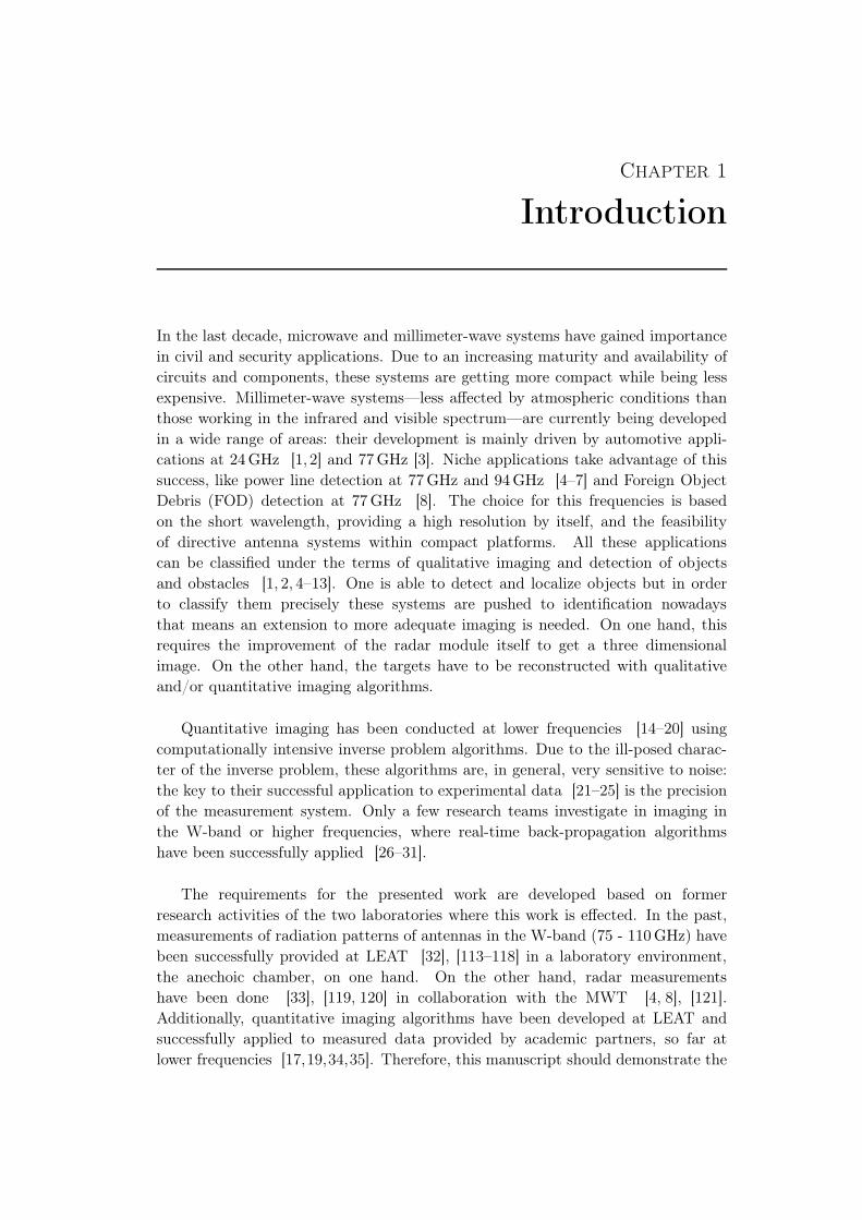
Fig. 2.1: Uniform plane wave incident on a cylindrical object. TM (left) and TE (right).
The problems described here are simplified to two-dimensional ones. Two-dimensional problems are those with invariance in the third dimension, such as aninfinite cylindrical structure illuminated by a field that does not vary along theaxis of the object. If the object axis lies along the z axis in a Cartesian coordinatesystem, it is convenient to separate the fields into Transverse Magnetic (TM) andTransverse Electric (TE) parts with respect to the variable z [38]. In practice, aproblem can be considered as two dimensional if all parameters of the media areconstant in z over several wavelengths. Many objects can be seen as 2D objectsin a first approach for mm-wave applications due to the short wave-length (forexample, power lines, pylons on the road etc). In general, objects are describedas 3D objects in three dimensions with a volume V. In the two-dimensional case,the object is described through its section S. One can classify the object in twocases depending on the polarization of the incident field: 2D-TE and 2D-TM. Thez-component of the electric field is absent in the TE case, while the z-component

6 Chapter 2. Electromagnetic Modeling
of the magnetic field is absent in the TM case (see Fig. 2.1). In the latter case,namely 2D-TM, all electric fields have only one component, the one in z-direction.This case is studied in detail and presented in this manuscript.
Circular cylinders represent one of the most important classes of geometricalsurfaces. The surface of many practical scatterers, for example the fuselage ofairplanes and missiles, can often be represented by cylindrical structures in a firstapproach. For us, they are of particular interest as the measurement system,presented in the next chapter, deals with circular cylinders so far. For them, thescattered fields can be exactly calculated with the analytic solution. This specialcase of circular cylinders is used in order to validate the numerical solution as wellas the measurement system.
y
x
D1 - "background"εr,1(r)σ1(r)D22
D21
ε′r,22(r)σ′22(r)
εr,21(r)σ21(r)
ε′2(r)ε′′2(r)
ε̃2(r)
D2 = D21 ∪ D22
k
⊙E(i)
H(i)
Fig. 2.2: Geometry of the problem.
The study of electromagnetics involves the application of Maxwell equations to aspecific geometry. The most general case is discussed below. Considering a source-free region of space (no charges, ρ = 0, and no currents, J = 0) containing aninhomogeneity characterized by a complex permittivity ε̃ (r) and a complex perme-ability µ̃ as shown in Fig. 2.2. If this region is illuminated by an electromagneticfield having the time dependence e jωt, the fields in the vicinity of the inhomogeneity

2.1. Introduction of the Problem 7
satisfy Maxwell equations:
∇×E + jωµ̃H =0 (2.1)
∇×H − jωε̃ (r)E =0 (2.2)
∇. (ε̃ (r)E) =0 (2.3)
∇. (µ̃H) =0 (2.4)
where E and H are the electric and magnetic fields, respectively. E and H arecomplex-valued and represent the vector amplitude and phase angle of the time-harmonic fields. Here, r represents the point of observation in space. Before solvingnumerically these equations, the definition of the complex permittivity and perme-ability should be closer discussed. Permittivity is a number related to the abilityof a material to propagate electromagnetic fields [39]. It is a quantity used to de-scribe dielectric properties that influence the reflection of electromagnetic waves atinterfaces and the attenuation of wave energy within materials. In the frequencydomain, the complex permittivity ε̃(r) (2.5) is defined with respect to the one of freespace ε0 (in F/m). With the complex permittivity ε̃(r), one can express the complexrelative permittivity ε̃r(r), also called dielectric constant, and define the complexwave vector:
ε̃(r) =ε0
(εr(r)− j
σ(r)
ωε0
)(2.5)
= ε′︸︷︷︸realpart
− j ε′′︸︷︷︸imaginary
part
ε̃r(r) =εr(r)− jσ(r)
ωε0(2.6)
k2(r) =ω2ε̃(r)µ0. (2.7)
The permittivity can be either expressed as a function of εr and σ, ε′ and ε′′ or in themost general case as complex value: ε̃. ε′ is defined as the real part of the dielectricpermittivity. It is complex when there is a delay between E and the polarizationP [40]. The imaginary part, ε′′, is proportional to the conductivity σ (in S/m). Theangular frequency ω is equal to 2πf . The real part ε′ is a measure of how muchenergy from an external electric field can be stored in a material. The dielectricloss factor ε′′, which is the imaginary part, influences the energy absorption and theattenuation. One more important parameter used in electromagnetic theory is thetangent of loss angle:
tan(δ) =ε′′
ε′. (2.8)
One can also define the complex permeability µ̃ which consists as well of a real part,that represents the energy storage and an imaginary part, that corresponds to theenergy loss term [41]. The relative permeability µ̃r is the absolute permeability µ̃
relative to the permeability of free space µ0. Some materials such as iron (ferrites),

8 Chapter 2. Electromagnetic Modeling
cobalt, nickel and their alloys have magnetic properties; however many materialsare non-magnetic. On the other hand, all materials have dielectric properties. Inthe following, it is assumed that µ̃ ∼ µ0. The values for a perfect conductor in themicrowave domain can be approximated for computation purposes [42] by: εr = 1,σ = ∞.
The geometry of interest for the application of the Maxwell equations (2.1)-(2.4) is shown in Fig. 2.2. The values indexed with 1 describe the homogeneousbackground media D1. The inhomogeneous scatterer D2, here described by anensemble of different homogeneous portions D21 and D22 exemplary, is completelysubmerged in the homogeneous background. In general, one can define the complexpermittivity for the whole area of interest as:
ε̃(r) =
{ε̃2 (r) , if r ∈ D2
ε̃1, if r /∈ D2.
Furthermore, one can define, with the complex relative permittivity (2.6), the con-trast C(r):
C(r) =
{ε̃r2(r)− ε̃r1 , if r ∈ D2
0, if r /∈ D2.(2.9)
A forward or direct scattering problem can be defined, in general, as the deter-mination of the scattered fields E(s)(r) everywhere, inside or outside the scattererD2, from known incident fields E(i)(r), scatterer and background media [43]. Thesuperposition of the incident and scattered fields yields the total field E(r) in thepresence of the scatterer:
E = E(i) +E(s). (2.10)
Its solution based on Maxwell equations is presented numerically in Section 2.2.1and analytically in Section 2.2.2.
An inverse scattering problem can be defined, in general, as the problem ofretrieving information about the scatterer from obtained scattered fields in a finitedomain, exterior to the scatterer D2, for known incident fields and backgroundmedium. The observation of the scattered fields might be carried out successivelywith different types of incident fields for different frequencies, different positionsof the sources and different locations of the receivers. The information about thescatterer could be any parameter which may characterize the scatterer, e. g. theshape (see Section 2.3.1) or the complex permittivity profile with its contrast asdemonstrated in Section 2.4.

2.2. Electromagnetic Modeling of the Direct Problem 9
2.2 Electromagnetic Modeling of the Direct Problem
2.2.1 Numerical Solution
The basis for the used methods, an integral representation of the electric field(EFIE) solved with a moment method solution, is briefly introduced in [44]and [45]. They have been continuously further developed for several differentapplications and configurations. Inverse problem algorithms have been investigatedin combination with a circular arrangement of emitters and receivers in [46] toreconstruct the complex permittivity profile of unknown objects based on simulatedand measured data. In [47], the polarimetric influence of scattered fields on thereconstruction of 2D buried objects has been studied. A boundary-oriented inversescattering method, based on contour deformations by means of level sets for radarimaging, has been presented in [48]. Furthermore, investigations have been done inmicrowave tomography for buried objects in two dimensions in [49] and extendedto three dimensions in [50] to mention only a few examples. The choice of themethods, due to its success in the past, is not explained in the presented work here,but its theory is summarized below.
Starting points are the Maxwell equations presented in (2.1)-(2.4). They are ap-plied to the problem described through the geometry shown in Fig. 2.2. In the caseof TM (Ez,Hx,Hy) the incident, the total and the scattered fields have only a com-ponent of the E-field in z-direction. The magnetic fields, however, have componentsin x- and y-directions which leads to:
∂Ez
∂y+ jωµ0Hx = 0 (2.11)
−∂Ez
∂x+ jωµ0Hy = 0 (2.12)
∂Hy
∂x− ∂Hx
∂y− jωε̃(x, y)Ez = 0 (2.13)
∂Hx
∂x+∂Hy
∂y= 0. (2.14)
Equations (2.11) and (2.12) are differentiated with respect to y and x respectivelyand merged. Finally, with (2.13) one obtains:
∂2Ez
∂x2+∂2Ez
∂y2+ ω2ε̃(x, y)µ0Ez = 0 (2.15)
which is equivalent to
∂2Ez
∂x2+∂2Ez
∂y2+ ω2ε̃1µ0Ez − ω2ε̃1µ0Ez + ω2ε̃(x, y)µ0Ez = 0
∂2Ez
∂x2+∂2Ez
∂y2+ ω2ε̃1µ0Ez = −ω2 (ε̃(x, y)− ε̃1)µ0Ez. (2.16)

10 Chapter 2. Electromagnetic Modeling
Assuming this, one can derive the equation of propagation (scalar Helmholtz equa-tion):
∆Ez + k21Ez =−(k2(x, y)− k21
)Ez (2.17)
k1 =ω√ε̃1µ0
k(x, y) =ω√ε̃(x, y)µ0.
A particular solution of the equation of propagation is given by:
Ez = G(k2(x, y)− k21
)Ez(x, y) (2.18)
where G is the impulse response also known as the Green’s function. The homoge-neous Helmholtz equation, that means without a right-hand-side term (without thepresence of an object), holds true for the incident fields. The general solution of theequation of propagation is:
Ez = E(i)z +G
(k2(x, y)− k21
)Ez. (2.19)
For an object in an arbitrary section D2 this leads to the following integral equation:
Ez(x, y) =E(i)z (x, y)
+
∫
D2
(k22(x, y) − k21
)G(x− x′, y − y′)Ez(x
′, y′)dx′dy′
∀(x, y) ∈ R2. (2.20)
One has to solve the following integral equation of the total field Ez(x, y) in thesection where r ∈ D2:
Ez(x, y)︸ ︷︷ ︸unknown
=E(i)z (x, y)︸ ︷︷ ︸
known
+
∫∫
D2
(k22(x
′, y′)− k21)
︸ ︷︷ ︸known
Ez(x′, y′)
︸ ︷︷ ︸unknown
G(x− x′, y − y′)︸ ︷︷ ︸
known
dx′dy′
︸ ︷︷ ︸E
(s)z (r) scattered field
(2.21)
Ez(x, y) = E(i)z (x, y) + E(s)
z (x, y). (2.22)
The domain of interest is discretized with N cells having the size of ∆x ×∆y (seeFig. 2.3). The pixels are addressed by rm and rn which are the points at the centerof the cell m and n respectively.
Ez(r) =E(i)z (r) +
∫ ∫
D2
(k22(r
′)− k21)Ez(r
′)G(r, r′)dr′
Ez(rm) =Eiz (rm) +
N∑
n=1
∫ ∫
Cn
(k22(rn)− k21
)Ez(rn)G(rm − rn)drn
︸ ︷︷ ︸scattered field of the nth pixel calculated at the point rm
. (2.23)
Finally, one can calculate the total field at one point which is the sum of the incidentfield and the integral, corresponding to the scattered field, at this point.

2.2. Electromagnetic Modeling of the Direct Problem 11
������������
������������
x
y
∆x
∆y
receivers
Cnrk (xk, yk)
rn (xn, yn)
rm (xm, ym)
section D2, object
Fig. 2.3: Discretization for numerical modeling.
Method of Moments
Equation (2.21) presents a Fredholm integral equation of the second kind as theunknown Ez(x, y) is inside and outside the integral. In this section, the Methodof Moments (MoM) is introduced. It is a numerical technique used to convertan integral equation into a linear system that can be solved numerically [52–54].Consider the general problem:
L(f) = g (2.24)
where L is a linear operator, which is equal to L = I −L′, with the identity I . Thefunction g is a known excitation source, also called forcing function, here the incidentfield, which corresponds to E(i)
z . The unknown function f is the total electric fieldEz.
L′ =
∫∫
D2
(k22(r
′)− k21)G(r, r′)dr′ (2.25)
L (Ez) = E(i)z . (2.26)
f is now expanded into a sum of N weighted basis functions,
EN(r) =
N∑
n=1
αnEn(r) (2.27)
N∑
n=1
αnL (En(r)) ≈ E(i)(r) (2.28)

12 Chapter 2. Electromagnetic Modeling
where αn are unknown weighting coefficients. An inner product or moment betweenthe basis function En and a testing or weighting function gm is defined as:
N∑
n=1
αn < L (En(r)) , gm >=< E(i)(r), gm > (2.29)
m = 1, · · · ,M.
The Dirac function δ(r−rm) has been chosen as testing function gm. This methodis referred to as point matching or collocation method:
δ(r − rm) =
{1, if r = rm
0, elsewhere.(2.30)
This collocation expresses an exact identity in the points rm.
N∑
n=1
αnL (En(rm)) = E(i)(rm) (2.31)
m = 1, · · · ,M.
Furthermore, a set of pulse functions have been chosen as basis functions:
En(r) = fn(r) (2.32)
fn(r) =
{1, if r ∈ Cn
0, if r /∈ Cn
(2.33)
αn = EN(rn) = E(rn). (2.34)
It is assumed that k2(r) is constant inside one pixel, that means k2(r) = k2(rn)
if rn is in Cn. Furthermore, one can express the integration over the Green’s functionby indexed elements Gmn which gives the following equations:
N∑
n=1
(δnm −
(k22(rn)− k21
) ∫∫
Cn
G(rm, rn)drn
)Ez(rn) = E(i)
z (rm) (2.35)
N∑
n=1
[Ez(rn)δmn −
(k22(rn)− k21
)Ez(rn)Gmn
]= E(i)
z (rm) .
With k20 = ω2ε0µ0 (k0 is the propagation constant in free space) and k2 = k20 ε̃rone can introduce the contrast C defined in (2.9):
N∑
n=1
[δmn − k20CnGmn
]En = E(i)
m with m = 1, · · · ,N. (2.36)

2.2. Electromagnetic Modeling of the Direct Problem 13
Finally, one can derive the matrix equation Ax = b with
Amn =δmn − k20CnGmn
x =En
b =
E(i)1...
E(i)N
A =I− GC with G = k20Gmn
A =
1− k20G11C1 −k20G12C2 · · ·−k20G21C1 1− k20G21C2
−k20G31C1. . .
1− k20GNNCN
. (2.37)
With the derived matrix equation one can calculate the total electric field inside thesection with an operator which acts on an internal field to produce an internal field:
GO = k20G
Omn. (2.38)
This is called the coupling equation and gives E. Then, the scattered field outside thesection, captured by receivers in the background D1, is calculated with G
RCE = E
(s).This equation is called the observation equation. The operator G
R. is defined asfollowed with respect to rk(xk, yk) (see Fig. 2.3):
GR = k20G
Rkn. (2.39)
Integral over the Green’s Functions
The integral over the Green’s function of R2 space is generally defined as:
Gmn =
∫
Cn
G (rm − rn) drn
=− j
4
∫
Cn
H(2)0 (k|rm − rn|) drn (2.40)
with H(2)0 the Hankel function of the second kind. Here, G (rm − rn) is the 2D
free-space Green’s function. Equation (2.40) has been calculated numerically onone hand. On the other hand, an approximation is presented, based on the com-mon standard approach [55]. For the case of receivers, located in the far-fieldof the scatterer, a far-field approximation of the object–receiver integral has beendeveloped.
Numerical Integration The object-object (Gmn) and object-receiver (Gkn)integrals over the Green’s function can be calculated numerically. For theobject-object case, one can distinguish the self element case (m = n) from the

14 Chapter 2. Electromagnetic Modeling
general case (m 6= n). Indeed, self elements represent a singularity since rm = rn
(see Fig. 2.3) but this singularity is integrable.
Gnn =
∫
Cn
G(x′, y′
)dx′dy′
=− j
4
∫ +∆
2
−∆
2
∫ +∆
2
−∆
2
H(2)0
(k1√x′2 + y′2
)dx′dy′ (2.41)
Gmn =
∫
Cn
G(xm − x′, ym − y′
)dx′dy′
=− j
4
∫ xn+∆
2
xn−∆
2
∫ yn+∆
2
yn−∆
2
H(2)0
(k1√
(xm − x′)2 + (ym − y′)2)dx′dy′ (2.42)
Gkn =
∫
Cn
G(xk − x′, yk − y′
)dx′dy′
=− j
4
∫ xn+∆
2
xn−∆
2
∫ yn+∆
2
yn−∆
2
H(2)0
(k1√
(xk − x′)2 + (yk − y′)2)dx′dy′. (2.43)
Standard Approach This approach is based on [55, 56]. For the object–objectintegral over the Green’s function with rm = rn one can write:
Gmm︸ ︷︷ ︸“self term“
= − jπ
2
1
k21
[Rk1H
(2)1 (Rk1)−
2 j
π
]. (2.44)
For the object–object or object–receiver integral respectively over the Green’s func-tion with rm or rk 6= rn one can write:
Gmn =− jπ
2H(2)
0 (k1|rm − rn|)R
k1J1 (Rk1) (2.45)
with R2 =∆x∆y
π=
∆2
π. (2.46)
The demonstration for (2.44) and (2.45) is shown in Appendix A.
Chosen Approximation Special care is taken for the calculation of the matrixself-elements [57, 58]. Following the standard approach, instead of integrating thesingular Green’s function over a square cell, we use a circular disk of equal area.However, this integration has been performed in an exact way: it is easy to showthat, for a polynomial of order three, the integral over the equivalent disk has tobe corrected by a factor of 3/π. One can further show that the integrands involvedin the self-elements are polynomials of order three for ordinary cell sizes. For theobject–object integral over the Green’s function with rm = rn one can write:
Gmm︸ ︷︷ ︸“self term“
= − 3
π
jπ
2
1
k21
[Rk1H
(2)1 (Rk1)−
2 j
π
]. (2.47)
2.2. Electromagnetic Modeling of the Direct Problem 15
For the object–object or object–receiver integral respectively over the Green’s func-tion with rm or rk 6= rn one can write:
Gmn =− 3
π
jπ
2H(2)
0 (k1|rm − rn|)R
k1J1 (Rk1) (2.48)
with R2 =∆x∆y
3. (2.49)
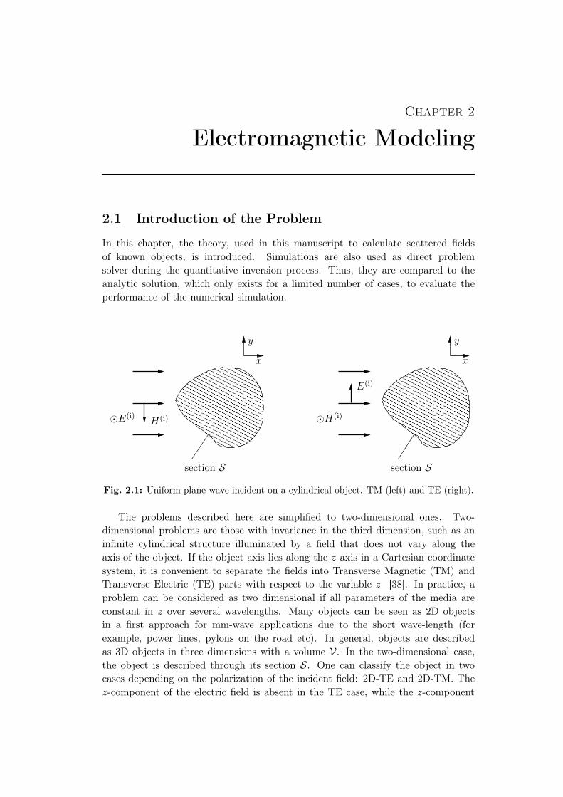
Far-Field Approximation The general case has already been shown and is pre-sented in order to define clearly the coordinates.
Esz =
∫∫
D2
G(r − r′
)C(r′)Ez
(r′)dr′
with G(r − r′
)= − j
4H(2)
0 (k1∣∣r − r′
∣∣)
r(x, y) and dr = dxdy
r(r, φ) and dr = rdrdφ.
y
x
r′
D2
r
φ
Fig. 2.4: Geometry of the far-field approximation.
H(2)0
(k1∣∣r − r′
∣∣) =H(2)0
(k1√r2 + r′2 − 2rr′ cos(φ− φ′)
)
where H(2)0 (ν) →
√2
πνe− j (ν−π
4) if ν → ∞.
With kr ≫ 1 and Taylor series [59], one can develop the Green’s function object–object:
G(r − r′
)≈ − j
4
√2
πk1re− j (k1r−π
4)e j k1(x
′ cos(φ)+y′ sin(φ)).

16 Chapter 2. Electromagnetic Modeling
In the far-field, for r → ∞, the scattered fields can be expressed by:
E(s)z (r, φ) ≈ e− j k1r
√r
F(φ) (2.50)
where the function F(φ) is called far-field pattern or scattered field pattern. Itdepends only on the angle φ. The radiation diagram and the presentation of |F (φ)|or |F (φ)|2 are generally expressed in dB. The center of the cells is taken as referencefor the fields, the contrast and the Green’s function. Doing so, one can finally obtainthe function F:
F(φ) =N∑
n=1
EnCnsinc
(k1
∆x
2cos(φ)
)
sinc
(k1
∆y
2sin(φ)
)
(− j
4
√2
πk1e j
π4
)e j k1(xi cosφ+yi sinφ)∆x∆y
︸ ︷︷ ︸G
. (2.51)
2.2.2 Analytic Solution
���������������������������������������������������������������������������������������������������������������������������������������������������������������������������������������������������������������������������������������
���������������������������������������������������������������������������������������������������������������������������������������������������������������������������������������������������������������������������������������
x
y
ε̃r, µrφ
ρ
a⊙E(i)
H(i)
k
Fig. 2.5: Uniform plane wave incident on a conducting or dielectric circular cylinder.
With the described methods one can simulate the scattered fields of complexnon-symmetric permittivity profiles. For certain electromagnetic scattering prob-lems, one can obtain analytical solutions. In the cylindrical coordinates, the so-lutions are expressed in the series form of the products of Bessel and exponentialfunctions. It serves to verify the implementations of the so far presented numer-ical methods to solve Maxwell equations in 2D. By comparison with the analyticsolution, investigations have been done for simulations of different discretization.The size of the squared cells determines mainly the approximation of the contourof the targets of interest. Additionally, the discretization by itself introduces, dueto a limited precision of the used machine, numerical noise. These effects have not

2.2. Electromagnetic Modeling of the Direct Problem 17
to be taken into consideration, at least much less significantly, by calculating theanalytic solution. The solutions to these problems are explained in detail in [60].The analytic solution is developed for the following cases:
• normal incidence plane wave scattering by conducting and dielectric circularcylinders,
• line source scattering by conducting and dielectric circular cylinders.
Here only the case of a plane wave scattered by a conducting cylinder and a dielectriccylinder is briefly introduced as it is used for comparison with the numerical simu-lations. The geometry is shown in Fig. 2.5 where a uniform plane wave is normallyincident upon a circular cylinder of radius a. The Balanis’ formula (e.g., chapter11 in [60]) has been modified to take into account the complex permittivity ε̃r of alossy homogeneous dielectric cylinder. The scattered fields can be written as:
E(s)z (ρ, φ) =E0
+∞∑
n=−∞αnH(2)
n (β0ρ) ejnφ (2.52)
αn = j−nJ′n (β0a) Jn
(β̃1a)−√
ε̃rµr
Jn (β0a) J′n(β̃1a)
√ε̃rµr
J′n(β̃1a)
H(2)n (β0a)− Jn
(β̃1a)
H(2)′
n (β0a)
with β̃1 =ω√µrε̃r
µr =1.
2.2.3 Description of the Means of Simulation
Flexible Method of Moments Code (FlexiMoM)
The first developed code is based on the Method of Moments. In its current form,this is a 2D-TM MoM, with a regular square mesh, pulse basis functions and point-matching. We have derived analytical expressions for the matrix elements (seeSubsection 2.2.1) and have compared these formulas with the results of numeri-cal integration, with no significant difference – except of course the computationtime (see Tab. B.2). More detailed results are shown in the Annex B.3. The code,called FlexiMoM, is written in Fortran 95/2003 [61]. Its architecture has beendesigned for flexibility, allowing easy maintenance and extension. The addition offeatures—e.g., various basis/test functions, mesh types, problem types (2D-TE, 3D),etc.—demands minor modifications of the code. We use Understand [62], a staticanalysis tool, and Lattix [63], an architecture analysis tool, to analyze and monitorthe source code during development. The objectives are: the code structure mustbe divided into modules, possible since Fortran 95/2003, which gives the possibilityfor a future parallelization of the code. The applications of interest, the softwarehas to be able to handle, are image reconstruction and detection through the wallon one hand. The so far presented theory of the direct problem solver is used to
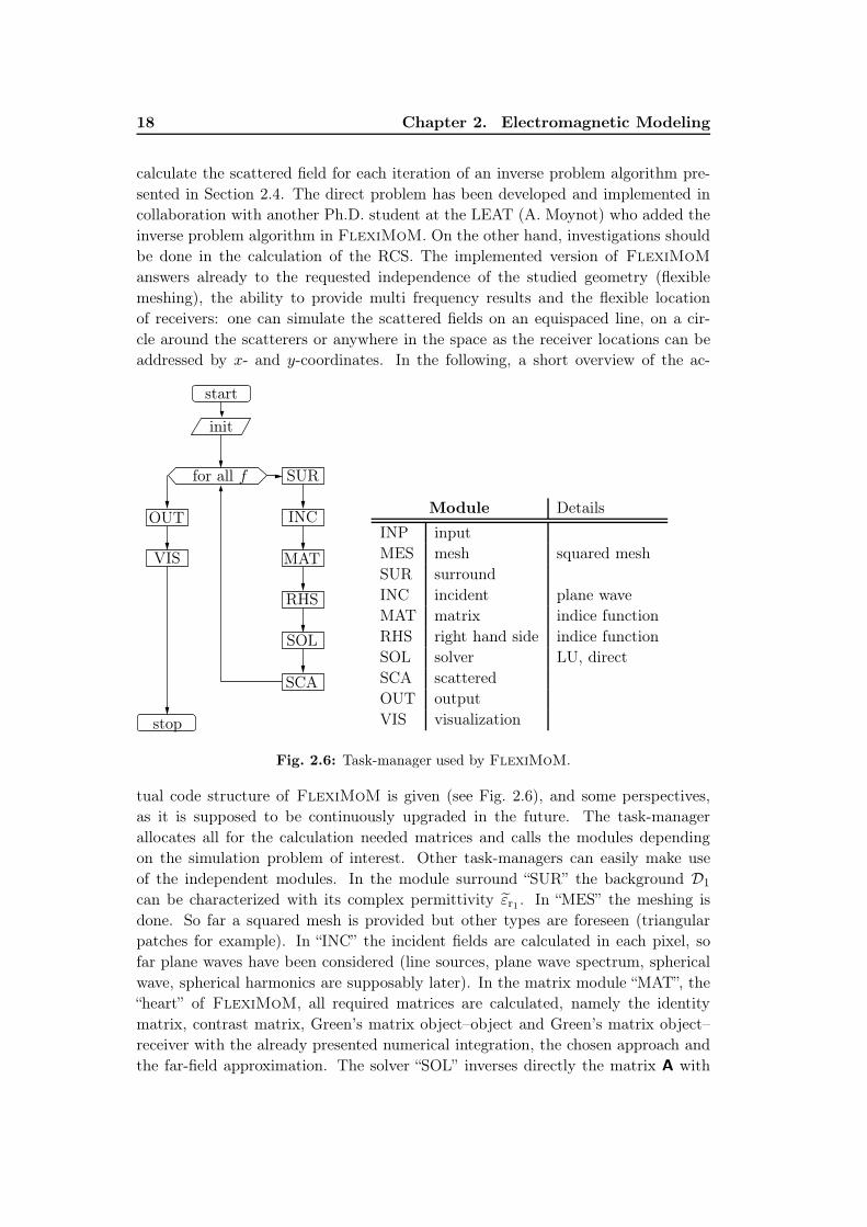
18 Chapter 2. Electromagnetic Modeling
calculate the scattered field for each iteration of an inverse problem algorithm pre-sented in Section 2.4. The direct problem has been developed and implemented incollaboration with another Ph.D. student at the LEAT (A. Moynot) who added theinverse problem algorithm in FlexiMoM. On the other hand, investigations shouldbe done in the calculation of the RCS. The implemented version of FlexiMoM
answers already to the requested independence of the studied geometry (flexiblemeshing), the ability to provide multi frequency results and the flexible locationof receivers: one can simulate the scattered fields on an equispaced line, on a cir-cle around the scatterers or anywhere in the space as the receiver locations can beaddressed by x- and y-coordinates. In the following, a short overview of the ac-
start
init
for all f SUR
INC
MAT
RHS
SOL
SCA
OUT
VIS
stop
Module Details
INP inputMES mesh squared meshSUR surroundINC incident plane waveMAT matrix indice functionRHS right hand side indice functionSOL solver LU, directSCA scatteredOUT outputVIS visualization
Fig. 2.6: Task-manager used by FlexiMoM.
tual code structure of FlexiMoM is given (see Fig. 2.6), and some perspectives,as it is supposed to be continuously upgraded in the future. The task-managerallocates all for the calculation needed matrices and calls the modules dependingon the simulation problem of interest. Other task-managers can easily make useof the independent modules. In the module surround “SUR” the background D1
can be characterized with its complex permittivity ε̃r1 . In “MES” the meshing isdone. So far a squared mesh is provided but other types are foreseen (triangularpatches for example). In “INC” the incident fields are calculated in each pixel, sofar plane waves have been considered (line sources, plane wave spectrum, sphericalwave, spherical harmonics are supposably later). In the matrix module “MAT”, the“heart” of FlexiMoM, all required matrices are calculated, namely the identitymatrix, contrast matrix, Green’s matrix object–object and Green’s matrix object–receiver with the already presented numerical integration, the chosen approach andthe far-field approximation. The solver “SOL” inverses directly the matrix A with

2.2. Electromagnetic Modeling of the Direct Problem 19
a LU decomposition [64]. Iterative methods can be used in the future to speed upthe calculation. A graphical visualization of the results after finishing the executionis provided by the visualization module with PLplot [65]. With FlexiMoM thescattered field of a metallic circular cylinder has been simulated with the chosenapproximation (2.48) and with the far-field approximation (2.50). The chosen pa-rameters for the simulation are summarized in Tab. 2.1. The amplitudes of thesimulated scattered fields are compared in Fig. 2.7. One can see that the simula-tion with the far-field approximation agrees perfectly with the simulation with thechosen approximation. Minor differences can be observed in the forward-scattereddirection.
Frequency f 1.0 GHz
Object: circular cylinder
radius 0.45 = 1.5λ0 m
position x = 0; y = 0; z = 0 m
εr 1.0
σ 100 MS/m
Domain of simulation
domainx = −1.5 · · · 1.5 m
y = −1.5 · · · 1.5 m
∆x 0.03 (λ0/10) m
∆y 0.03 (λ0/10) m
Receiver position radius 6.0 = 20λ0 m
on a circle ∆φ 2.0 degrees
Tab. 2.1: Parameters of simulation to compare the scattered field for simulated, with the
chosen approximation and with the far-field approximation, results.

20 Chapter 2. Electromagnetic Modeling
0.8
0.6
0.4
0.2
0
0.2
0.4
0.6
0.8
0.8 0.6 0.4 0.2 0 0.2 0.4 0.6 0.8
Amplitude
k
chosen approximationfar-field approximation
Fig. 2.7: Amplitude of the scattered field at points of receivers. Simulation of the scat-
tered field with the chosen approximation (2.48) and with the far-field approxi-
mation (2.50).
Electromagnetic SCattering AnaLytic codE (Escale)
The second code, Escale, is a set of GNU Octave [66] scripts that provides aversatile interface to analytic solutions of scattering problems. It has been developedand implemented by a researcher at the LEAT (I. Aliferis).In its current version, Escale calculates the electric scattered field by a PerfectElectric Conductor PEC or dielectric cylinder (ideal or with ohmic losses) underplane-wave or line-source illumination, based on analytic (closed-form) expressionsas partly presented in Subsection 2.2.2. The infinite series are calculated term byterm, till convergence to the numerical precision of the machine is achieved. Moreproblem types will be added in the future.
Comparison with Numerical Results
As a preliminary step to the following chapter on measurements, we present herea comparison between numerical results obtained with the MoM and the analyticsolution in the case of plane-wave scattering by two PEC cylinders and a dielectriccylinder at 92.5GHz, the center frequency of the W-band. For simulations withFlexiMoM, the area of the object of interest has to be discretized. The choice ofthe discretization is a trade off between calculation time and approach to the exactsolution. As high the area of simulation is discretized, the longer the simulation takes
2.2. Electromagnetic Modeling of the Direct Problem 21
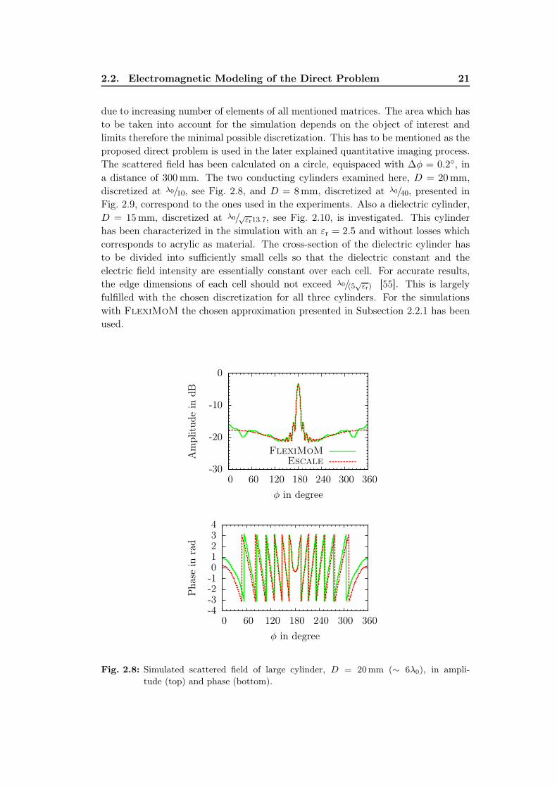
due to increasing number of elements of all mentioned matrices. The area which hasto be taken into account for the simulation depends on the object of interest andlimits therefore the minimal possible discretization. This has to be mentioned as theproposed direct problem is used in the later explained quantitative imaging process.The scattered field has been calculated on a circle, equispaced with ∆φ = 0.2◦, ina distance of 300mm. The two conducting cylinders examined here, D = 20mm,discretized at λ0/10, see Fig. 2.8, and D = 8mm, discretized at λ0/40, presented inFig. 2.9, correspond to the ones used in the experiments. Also a dielectric cylinder,D = 15mm, discretized at λ0/√εr13.7, see Fig. 2.10, is investigated. This cylinderhas been characterized in the simulation with an εr = 2.5 and without losses whichcorresponds to acrylic as material. The cross-section of the dielectric cylinder hasto be divided into sufficiently small cells so that the dielectric constant and theelectric field intensity are essentially constant over each cell. For accurate results,the edge dimensions of each cell should not exceed λ0/(5√εr) [55]. This is largelyfulfilled with the chosen discretization for all three cylinders. For the simulationswith FlexiMoM the chosen approximation presented in Subsection 2.2.1 has beenused.
-30
-20
-10
0
0 60 120 180 240 300 360
Am
plitud
ein
dB
φ in degree
FlexiMoMEscale
-4-3-2-101234
0 60 120 180 240 300 360
Pha
sein
rad
φ in degree
Fig. 2.8: Simulated scattered field of large cylinder, D = 20mm (∼ 6λ0), in ampli-
tude (top) and phase (bottom).

22 Chapter 2. Electromagnetic Modeling
-30
-20
-10
0 60 120 180 240 300 360
Am
plitud
ein
dB
φ in degree
FlexiMoMEscale
-4-3-2-101234
0 60 120 180 240 300 360
Pha
sein
rad
φ in degree
Fig. 2.9: Simulated scattered field of small cylinder, D = 8mm (∼ 2.5λ0), in ampli-
tude (top) and phase (bottom).

2.2. Electromagnetic Modeling of the Direct Problem 23
-70-60-50-40-30-20-10
0
0 60 120 180 240 300 360
Am
plitud
ein
dB
φ in degree
FlexiMoMEscale
-4-3-2-101234
0 60 120 180 240 300 360
Pha
sein
rad
φ in degree
Fig. 2.10: Simulated scattered field of dielectric cylinder, D = 15mm (∼ 4.5λ0), in ampli-
tude (top) and phase (bottom).
As seen in the results, FlexiMoM fits well Escale, especially in the case ofthe small cylinder which is discretized at a higher precision. Some discrepanciesin amplitude and in phase are present in the back-scattered region, due to theapproximate (staircase) description of the cylinder’s contour. This becomes morecritical there for the comparison in phase of the dielectric cylinder.
Definition of the Signal-to-Noise Ratio
Before going further, the differences between the exact solution and the numericalsimulation should be discussed more in detail. This difference can be estimated byusing the same equation as for calculating the Signal-to-Noise Ratio (SNR) [67]based on the error e:
e =
⟨E
(s)sim. − E
(s)exact, E
(s)sim. − E
(s)exact
⟩
⟨E
(s)exact, E
(s)exact
⟩ (2.53)
SNR
∣∣∣∣dB
=− 10 log (e) . (2.54)

24 Chapter 2. Electromagnetic Modeling
The reference signal is the analytic solution E(s)exact from Escale. The error between
the analytic solution and the numerical solution is the numerical noise introduced bythe latter one. This difference depends on several choices made for the simulation,namely the size of the area taken into consideration for the simulation and the sizeof the cells (∆). The discretization, that means the cell size, influences mainly the“error” of the numerical approach and results in a limited SNR. In the following,the SNR has been calculated for the three cylinders presented in this chapter andsummarized in Tab. 2.2. The angular range φ ∈ [30 · · · 330] has been taken intoconsideration in order to be in conditions imposed by the measurement systempresented in Chapter 3.
∆SNR in dB
75GHz 92.5GHz 110GHz
Metallic cylinder
D = 20mm λ0,min/9.1 8.36 6.49 (Fig. 2.8) 5.03
D = 8mmλ0,min/34.1 20.73 18.81 (Fig. 2.9) 17.23
λ0,min/9.1 8.65 6.83 5.36
Dielectric cylinder
D = 15mm λ0,min/√2.511.5 7.78 13.88 (Fig. 2.10) 8.50
Tab. 2.2: SNR for 1501 points of the numerical simulation with FlexiMoM.
One can see that the SNR depends mainly on the chosen discretization ∆. Forthe metal targets, the results show that the SNR decreases when the frequencyincreases for a constant discretization. This is not the case for the dielectriccylinder. The best SNR occurs at the center frequency but is worse for thelowest/highest frequency (7.78 dB/8.50 dB). In the future, further investigationsare going to be done in studying the SNR for different dielectric targets as functionof the pixel size ∆ in the W-band.

2.3. Qualitative Imaging - Localization and Shaping 25
2.3 Qualitative Imaging - Localization and Shaping
The term of qualitative imaging refers more or less to the representation of a pa-rameter which cannot be related in a simple manner or quantitatively to a physicalone or which is a non linear function of several physical parameters (as the electriccurrent distribution inside the scatter) but depends on the scatterer. Despite of this,the mapping of variations of the parameter can be of practical interest [43]. Thelocalization and shaping of the targets is investigated and explained in detail in thefollowing. This is done with the back-propagation of the scattered fields. Two caseshave been studied: on one hand back-propagation of scattered fields in combinationwith incident plane wave sources as primary sources has been done. This is relatedto a circular configuration of several receivers pointed to the target of interest. Onthe other hand back-propagation is applied with scattered fields and the incidentfields of only two emitters which act in the same time as receivers. Therefore, theprimary source is assumed to be a line source.
2.3.1 Back-propagation - Monochromatic Approach
The scattered field E(s) can be calculated with the matrix equation as shown in
Section 2.2.1:
E(s) = G
RCE (2.55)
where GR is the matrix of the Green’s function object–receiver, C presents the
contrast and E the total fields inside the section.The goal is to recalculate CE, also called the contrast source, based on simulated ormeasured scattered fields E
(s). One could think about(G
R)−1
E(d) = CE, but the
matrix(G
R)−1
cannot be calculated as it is not squared.
That’s why in [19] a matrix GR∗
= GRt
, which is the transposed conjugate ofG
R, has been used as initial guess for an inverse problem algorithm. With thismatrix the scattered fields can be back propagated to get a field distribution S(x, y)proportional to the polarization current in the target Jp:
S(x, y) = GR∗
Es =G
R∗G
RCE
⋍γICE
(2.56)
where Jp = CE. The matrix multiplication GR∗
GR gives not exactly the identity
matrix. Therefore, γ ∈ R is introduced as a scaling factor to obtain GR∗
GR⋍ γI.
The elements of the matrix CE, which was used to simulate the scattered fieldsof the conducting cylinder of D = 20mm in the Section 2.2.3, are visualized inFig. 2.12. The results are compared with the image S(x, y) obtained with theback-propagation via the matrix G
R∗. The configuration for the back-propagation
is shown in Fig. 2.11.

26 Chapter 2. Electromagnetic Modeling
The discrepancies are due to the matrix GR∗
which is not a unitary matrix.
x
y
E(s)(xm, ym, f, E
(i))
targetS(x, y)
r0
dm
Fig. 2.11: Configuration assumed to back-propagate the scattered fields.
In the following the matrix product GR∗
Es is approximated with the following
incoherent sum over all receivers m = 1, · · · ,M:
S(x, y) =1
F1
L1
M
F∑
f=1
L∑
l=1
∣∣∣∣∣
M∑
m=1
√dmE
(s)(xm, ym, f, E
(i)m
)e j [Φ(x,y,xm,ym,f)]
∣∣∣∣∣ . (2.57)
The shift in phase Φ (x, y, xm, ym, f) depends on the geometry of the cells and thereceiver positions and has to be calculated for each frequency and each emitter re-spectively. The emitter represents the primary source which can be replaced bythe polarization currents in the objects (primary sources are replaced by secondarysources). A configuration with several emitters is taken into account by the incoher-ent sum in the presented approach. The images obtained for each emitter separatelyare summed up to retrieve the shape of the object. Therefore, the modules are sep-arately summed up for all emitters l = 1, · · · ,L and frequencies f = 1, · · · ,F. Thederived sum is based on the similarity with the far-field approximation presentedin 2.2.1. The general configuration is visualized in Fig. 2.11. The scattered fieldE(s)
(xm, ym, f, E
(i))
depends on the coordinates of the receiver and is calculated orsimulated for each frequency and each emitter position respectively.

2.3. Qualitative Imaging - Localization and Shaping 27
Nor
mal
ized
mag
nitu
de
yin
mm
x in mm
0
0.2
0.4
0.6
0.8
1
-10
-5
0
5
10
-10 -5 0 5 10
Nor
mal
ized
mag
nitu
de
yin
mm
x in mm
0.10.20.30.40.50.60.70.80.91
-10
-5
0
5
10
-10 -5 0 5 10
Fig. 2.12: Normalized magnitude of CE used in the direct problem calculations (top) and
the module of the product S(x, y) = GR∗
Es after back-propagation (bottom)
with r0 = 300mm.
28 Chapter 2. Electromagnetic Modeling
2.3.2 Back-propagation - Multifrequency Approach
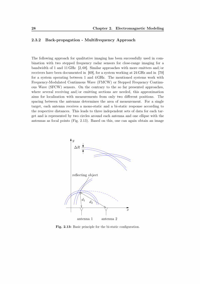
The following approach for qualitative imaging has been successfully used in com-bination with two stepped frequency radar sensors for close-range imaging for abandwidth of 1 and 11GHz [2, 68]. Similar approaches with more emitters and/orreceivers have been documented in [69], for a system working at 24GHz and in [70]for a system operating between 1 and 4GHz. The mentioned systems work withFrequency-Modulated Continuous Wave (FMCW) or Stepped Frequency Continu-ous Wave (SFCW) sensors. On the contrary to the so far presented approaches,where several receiving and/or emitting sections are needed, this approximationaims for localization with measurements from only two different positions. Thespacing between the antennas determines the area of measurement. For a singletarget, each antenna receives a mono-static and a bi-static response according tothe respective distances. This leads to three independent sets of data for each tar-get and is represented by two circles around each antenna and one ellipse with theantennas as focal points (Fig. 2.13). Based on this, one can again obtain an image
x
y
reflecting object
antenna 1 antenna 2
d1 d2
∆R
Fig. 2.13: Basic principle for the bi-static configuration.

2.3. Qualitative Imaging - Localization and Shaping 29
S(x, y):
S(x, y) =
d1(x, y)
F∑
f=1
E(s)1f e
j 2kfd1(x,y)
·
d2(x, y)
F∑
f=1
E(s)2f e
j 2kfd2(x,y)
·
√d1(x, y)d2(x, y)
F∑
f=1
E(s)12f e
j kf (d1(x,y)+d2(x,y))
(2.58)
where S(x, y) is the amplitude from a possible target at the point (x, y). The dis-tance between one cell of the image and the first or second antenna is indicatedwith d1(x, y) and d2(x, y) respectively. The scattered field E
(s)1f is the mono-static
response of the first and E(s)2f the mono-static responses of the second antenna. The
field E(s)12f corresponds to the bi-static response which is reciprocal to E
(s)21f . This
leads to the circular and elliptical locus curves shown in Fig. 2.13. In the far-field ofthe antennas, one can suppose a two dimensional arrangement with an amplitudedependency of 1/√r (see (2.50)). That’s why the range-dependent amplitude cor-rection is done with the factor d1(x, y) and d2(x, y). Again, a summation over allfrequencies for f = 1, · · · ,F is done. The longitudinal resolution can be specifiedas:
∆R =c0
2∆f(2.59)
where ∆f corresponds to the frequency bandwidth of operation. The lateral reso-lution decreases with the distance to the both antennas as the intersections of thecircles become larger.

30 Chapter 2. Electromagnetic Modeling
2.4 Quantitative Imaging - Reconstruction of the Com-
plex Permittivity
On the contrary to qualitative imaging, quantitative imaging retrieves a quantita-tive value of a physical parameter. In the following description, the reconstructionof the complex permittivity ε̃r is investigated.
The following results have been obtained in collaboration with a Ph.D. studentat the LEAT (A. Moynot). He is in charge of the development and implementationof the inverse problem. The goal has been to provide measurements which can besuccessfully used for quantitative imaging. Hereafter, the general principles of theused algorithm are briefly concluded.
2.4.1 Description of the Inversion Algorithm
The inverse scattering problem of reconstructing the complex permittivity profileof 2D or 3D metallic or dielectric objects is a well-known ill-posed and nonlinearproblem, i.e. in the sense of Hadamard [71]. The existence, uniqueness and sta-bility of the solution are not simultaneously ensured. Starting from an integralrepresentation of the electric field (EFIE), as explained in detail in Section 2.2.3, aniterative algorithm has been developed based on a bi-conjugate gradient method forreconstructing the relative permittivity and conductivity (i.e. complex permittivityprofile) of a Target Under Test (TUT). We assume that the two-dimensional objectis contained in a bounded domain D1 (see Fig. 2.2) and irradiated successively byL different known incident fields. For each excitation l = 1, · · · ,L, the scatteredfields are measured by a set of receivers. Starting from the domain integral equationfor the total fields inside D2 and from the integral representation of the scatteredfields on the measurement points (2.36), the moment method yields the followingnonlinear matrix system:
E(s)l = G
RC(I− G
OC)−1
E(i)l (2.60)
where E(s)l represents the scattered field vector and E
(i)l the incident field vector. We
consider the real and imaginary part of the contrast C as independent variables. Thesolution of the inverse scattering problem is given by minimizing the cost functionalJ(C) representing the error matching the measured scattered fields E
(s)l,meas. and the
computed one E(s)l,comp. for a given contrast C:
J(C) =L∑
l=1
∥∥∥E(s)l,meas. − E
(s)l,comp.
∥∥∥2. (2.61)
The inversion algorithm is based on a conjugate gradient method [19] for thereal part and the imaginary part of the contrast C and a Polak-Ribière conjugate
2.4. Quantitative Imaging - Reconstruction of the ComplexPermittivity 31
gradient direction. The gradient direction is determined by calculating the Fréchetderivative of the cost functional J(C). The described method can be, in principle,applied to any kind of lossy dielectric objects with near-field as well as far-field data.
In the following, the inverse problem algorithm has been applied to simulatedscattered fields. So far, no regularization has been investigated. In this manuscriptonly the quantitative reconstruction of metallic objects is of interest. For the inver-sion of scattered fields from dielectric objects a regularization scheme is necessary.
2.4.2 Quantitative Imaging Performance for Metallic Objects
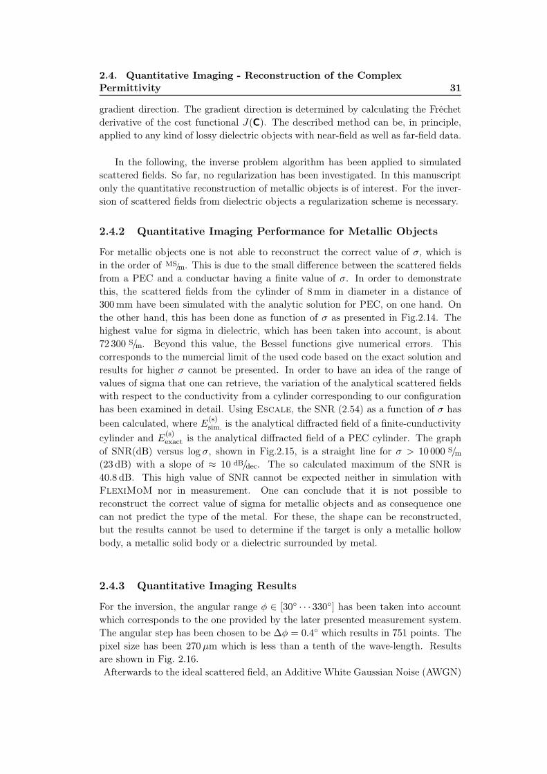
For metallic objects one is not able to reconstruct the correct value of σ, which isin the order of MS/m. This is due to the small difference between the scattered fieldsfrom a PEC and a conductar having a finite value of σ. In order to demonstratethis, the scattered fields from the cylinder of 8mm in diameter in a distance of300mm have been simulated with the analytic solution for PEC, on one hand. Onthe other hand, this has been done as function of σ as presented in Fig.2.14. Thehighest value for sigma in dielectric, which has been taken into account, is about72 300 S/m. Beyond this value, the Bessel functions give numerical errors. Thiscorresponds to the numercial limit of the used code based on the exact solution andresults for higher σ cannot be presented. In order to have an idea of the range ofvalues of sigma that one can retrieve, the variation of the analytical scattered fieldswith respect to the conductivity from a cylinder corresponding to our configurationhas been examined in detail. Using Escale, the SNR (2.54) as a function of σ has
been calculated, where E(s)sim. is the analytical diffracted field of a finite-cunductivity
cylinder and E(s)exact is the analytical diffracted field of a PEC cylinder. The graph
of SNR(dB) versus log σ, shown in Fig.2.15, is a straight line for σ > 10 000 S/m(23 dB) with a slope of ≈ 10 dB/dec. The so calculated maximum of the SNR is40.8 dB. This high value of SNR cannot be expected neither in simulation withFlexiMoM nor in measurement. One can conclude that it is not possible toreconstruct the correct value of sigma for metallic objects and as consequence onecan not predict the type of the metal. For these, the shape can be reconstructed,but the results cannot be used to determine if the target is only a metallic hollowbody, a metallic solid body or a dielectric surrounded by metal.
2.4.3 Quantitative Imaging Results
For the inversion, the angular range φ ∈ [30◦ · · · 330◦] has been taken into accountwhich corresponds to the one provided by the later presented measurement system.The angular step has been chosen to be ∆φ = 0.4◦ which results in 751 points. Thepixel size has been 270 µm which is less than a tenth of the wave-length. Resultsare shown in Fig. 2.16.Afterwards to the ideal scattered field, an Additive White Gaussian Noise (AWGN)

32 Chapter 2. Electromagnetic Modeling
-35
-30
-25
-20
-15
-10
-5
50 100 150 200 250 300
Am
plitud
ein
dB
φ in degree
PECfinite conductivity
PEC
10
2550100
10001000072300
Fig. 2.14: Comparison of scattered fields from PEC and finite sigma conductor for a cylin-
der of 8mm in diameter, simulated in a distance of 300mm for f = 110GHz.
has been added to obtain a SNR of 5 dB. The cost function, shown in Fig. 2.18, ishigher for the noised case than for the ideal one. Anyway, the cylinder contour couldbe perfectly retrieved. Knowing this, one can apply the presented inverse problemalgorithm to noised measurements as presented in Chapter 4.2.
00.10.20.30.40.50.60.70.80.9
1
0 10 20 30 40 50 60 70 80 90100
Nor
mal
ized
cost
valu
e
Iterations
idealnoisy
Fig. 2.18: Normalized cost values for each iteration obtained for 92.5GHz. Scattered fields
have been simulated with Escale ideal and with a SNR=5 dB.

2.4. Quantitative Imaging - Reconstruction of the ComplexPermittivity 33
0
10
20
30
40
50
101 102 103 104 105
SNR
indB
Conductivity in S/m
Fig. 2.15: Comparison of scattered field from a cylinder with D = 8mm for a frequency
of f = 110GHz: sigma-PEC SNR versus finite sigma.
yin
mm
x in mm
yin
mm
x in mm
11.021.041.061.081.11.121.141.161.181.2
-4-3-2-101234
-4 -3 -2 -1 0 1 2 3 4
εr
-4-3-2-101234
-4 -3 -2 -1 0 1 2 3 4
εr
x in mmx in mm
0
2
4
6
8
10
12
-4 -3 -2 -1 0 1 2 3 4
σ in S/m
-4 -3 -2 -1 0 1 2 3 4
σ in S/m
Fig. 2.16: The relative permittivity (left) and the conductivity (right) reconstructed
with 100 iterations (751 receivers, 1 emitter, 92.5GHz, discretization with
0.27mm ≈ λ0,min/10). Scattered field of the cylinder, D = 8mm, has been sim-
ulated with Escale for a distance of 300mm.

34 Chapter 2. Electromagnetic Modeling
yin
mm
x in mm
yin
mm
x in mm
11.021.041.061.081.11.121.141.161.181.2
-4-3-2-101234
-4 -3 -2 -1 0 1 2 3 4
εr
-4-3-2-101234
-4 -3 -2 -1 0 1 2 3 4
εr
x in mmx in mm
0
2
4
6
8
10
12
-4 -3 -2 -1 0 1 2 3 4
σ in S/m
-4 -3 -2 -1 0 1 2 3 4
σ in S/m
Fig. 2.17: The relative permittivity (left) and the conductivity (right) reconstructed
with 100 iterations (751 receivers, 1 emitter, 92.5GHz, discretization with
0.27mm ≈ λ0,min/10). Scattered field of the cylinder, D = 8mm, has been sim-
ulated with Escale for a distance of 300mm with a SNR=5 dB.
Chapter 3
Scattered Field Measurement
System for Imaging with
mm-Waves
3.1 Comparison of Existing Systems
In this section a short description of the existing Scattered Field Measurement Sys-tems (SFMS) is given. The references in [72] have been concluded and supple-mented. Firstly, measurement facilities providing measurements in one plane areintroduced. Secondly, systems operating on a sphere to obtain 3D field measure-ments are presented. These systems aim to provide accurate measurements to theinverse problem community. Also a last type of systems of an area becoming of in-creasing interest is going to be mentioned: Compact Antenna Test Ranges (CATR)that provide measurements of the radiation patterns of antennas in the W-band.They could be good candidates to be used as well for scattered field measurements,minor modifications and extensions assumed, as they aim to provide high precisionand accuracy.
3.1.1 Two Dimensional Scattered Field Measurement Facilities
The following systems are developed to measure the amplitude of scattered fieldsto obtain the RCS of targets of interest. The systems described below providemeasurements with a bi-static circular configuration:
• The automated swept-angle bi-static scattering measurement system of theRome Laboratory, NY, USA, [25] has been installed to obtain reliablemeasurements on canonical scatterers. The frequency of operation is in the S-,C- and X-bands (2GHz to 12.4GHz). Measurements, also known as Ipswich
Data [73], have been successfully used for inversion and resulted in numerouspublications like [17], [19] and [20] to mention only a few. The targetsare mounted rotatable in the center of the system and the receive antennasweeps to collect data as a direct function of the bi-static angle. The stepsize of the angle is 0.2◦ and the system is able to measure “on the fly” over anobservation sector of 180◦. The distance from the target to the aperture of thereceive antenna is about 3.0m and from the target to the emitting antennais 3.7m to measure in the far-field zone of the scatterers. Investigations havebeen done with 15.24 cm dish antennas in an anechoic chamber.

36Chapter 3. Scattered Field Measurement System for Imaging with
mm-Waves
• The anechoic facility “BABI” of the Office National d’Etudes et de RechercheAérospatiales (Onera), Châtillon, France, [74] provides bi-static RCS valuesof airborne targets. Measurements are possible in the L-, S-, C-, X- and Ku-bands (1GHz to 18GHz). The target is also fixed in the center of rotationwhere it can be turned on its own axis. Measurements are done over almost160◦ in 0.5◦ steps. The distance between the center and the emitting andreceiving modules are 5.5m respectively. The used antennas are wide-bandbi-polarized horn antennas.
• The measurement system “CACTUS”, of the Centre d’Etudes Scien-
tifique et Techniques d’Aquitaine (CESTA), Barp, France, [75] isclosed in configuration to “BABI”. Measurements are investigated in stealthtechnology of military targets. The frequencies of interest are in the S-, C-, X-and Ku-bands (2GHz to 18GHz). Measurements can be done over 180◦. Thedistance between the emitting section and the target is 5.6m. The system isinstalled in an anechoic chamber.
• The University of Florida’s Laboratory for Astrophysics, FL,USA, [21] implemented a microwave scattering facility to test theoreticalsolutions to electromagnetic scattering problems of particles. The frequencyof operation is in the W-band (75GHz to 110GHz). Measurements are pro-vided, with a step size of 0.1◦, from 0◦ to 168◦ where the latter corresponds tothe forward scattering direction. The distance between the antennas and thecenter of the target is 1.35m. Full band-with conical horn antennas in combi-nation with Fresnel lenses are used to obtain far-field conditions. Mentionableis the given mechanical and thermal stability of 10µm. The facility is locatedin a chamber dedicated to this type of measurement.
• The Institut Fresnel, Marseille, France, [24] provides a database to theinverse problem community to test inversion algorithms against experimentaldata. These are obtained in the S-, C-, X- and Ku-bands (2GHz to 18GHz).Measurements in a two-dimensional configuration have been done on a circlefrom 60◦ to 300◦ with a step-size of 1.0◦. The source-object center and objectcenter-receiver distances are 1.67m. The transmitting and receiving antennasare both wide-band ridged horn antennas. In order to provide measured fieldsin an electromagnetic free space configuration the whole system is installed inan anechoic chamber.
3.1.2 Measurement Systems Providing Three Dimensional Results
• The Institut Fresnel, Marseille, France, [24] has continued providing newmeasurement results also of three dimensional targets (see [23]). With theconfiguration presented in [76] the sources have been moved from −160◦ to160◦ with a step of 40◦ in the azimuthal direction and from 30◦ to 160◦ witha step of 10◦ in the elevation direction. The receivers are restricted to the

3.1. Comparison of Existing Systems 37
equatorial plane and moving from −180◦ to 180◦, with a step of 5◦, and withan exclusion of 50◦ on both sides of the source meridian.
• The European Microwave Signature Laboratory, Ispra, Italy, [77] isa facility to conduct research in performing mono- and bi-static polarimetricradar measurements in a stable, controlled and reproducible way in an anechoicchamber of 20m in diameter. The basic measurement system can be used inthe L-, S-, C-, X-, Ku-, K- and Ka-bands (1GHz to 40GHz). The targets arerotatable of 360◦. Two radar transmitters/receivers can be moved on a circlearound the targets in a distance of 10m from −115◦ to 115◦ with a precisionof ±0.005◦.
• The University of Michigan, MI, USA, [78] constructed a polarimetricbi-static radar facility to serve as a research tool for improved understandingof the nature of bi-static scattering for point and distributed targets. Thesystem works at 10GHz, 35GHz and 94GHz. The transmitter, a dish an-tenna, has two degrees of positional freedom, capable of moving in both theelevation plane (over 90◦) and the azimuthal one (over 360◦). The receiver,a horn antenna, can be positioned in the elevation plane (over 90◦). The po-sitional accuracy is given with ±0.1◦. The distances between the center andthe aperture of the transmitter and the aperture of the emitter are 2.01m and3.26m, respectively.
3.1.3 Compact Range Antenna Facilities
Systems facing the same challenges in point of view of mechanical limitations dueto high frequencies are presented here. The increase in frequency adds additionalrequirements to the accuracy of the mechanical positioning devices required to movethe probe and antenna under test.
• The MI Technologies, GA, USA, [79] has constructed a spherical near-field arch positioner with a 1.5m radius to support measurements requiringaccurate knowledge of the probe phase center within 64µm throughout itsrange of travel.
• The European Space Agency, Noordwijk, Netherlands, [80] investigatesin modeling the variation of atmospheric variables (humidity, temperature andpressure) on all the elements of a CATR facility used for mm-wave measure-ments.

38Chapter 3. Scattered Field Measurement System for Imaging with
mm-Waves
3.2 Description of the Measurement System
3.2.1 Introduction of Objectives
A SFMS consists in placing the TUT at the center of one or two motorized circularrails or swivel arms, depending weather 2D or 3D measurements are performed.Horn antennas are generally used as illuminator and receiver. Most of time, instal-lations are fixed in dedicated anechoic chambers as the mentioned examples haveshown. The solution proposed in this manuscript is quite different. The SFMS hasbeen developed with four main objectives:
1. being fully compatible with the actual antenna measurement system installedat the LEAT,
2. being low-cost,
3. reducing as much as possible the positioning errors due to the high frequency,
4. measuring 2D objects.
The first condition is very important for users whose anechoic chamber is mainlydedicated to antenna measurements. It implies that the system should be easyto remove. The second condition shall meet the requirement of an inexpensivemechanical extension to the already existing chamber (8.7m × 4.3m × 4.0m) andits measurement devices [81]. The last condition drove our choice toward anoverall small size system that is also coherent with the short wavelength value. Theoriginal measurement system is used to obtain the radiation pattern of antennasfrom 820MHz to 50GHz and from 75 to 110GHz. The existing equipment meetsall major requirements in already implemented soft- and hard-ware for the latermentioned purposes and has the advantage that interferences from the surroundingsare suppressed by pyramidal absorbers (FPY205/310/470) [82]. One has tomention that the results which are presented in the following were obtained duringone single series of measurements. This lasted only one week as the anechoicchamber had been booked by other researchers.
3.2.2 Description of Mechanical Modifications
The technical details are summarized in Tab. 3.1 and explained hereafter. In Fig. 3.1the planned system with its additional installed parts and the following describedmodifications are shown. The emitting section is separated from the first tower andlocated in a distance of 400mm between the antenna and the center of the secondtower to ensure that the target is located in the far-field of the emitting antenna.The receiving part, displaced as well from its origin on the second turntower, islocated on an additional swivel arm. The distance between the receiver and thecenter (300mm) has been chosen to be as small as possible. At 110GHz the 2D2/λ0
far-field requirement limits the maximum target dimension to about 20mm. Indeed,
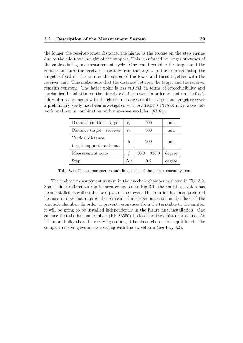
3.2. Description of the Measurement System 39
the longer the receiver-tower distance, the higher is the torque on the step enginedue to the additional weight of the support. This is enforced by longer stretches ofthe cables during one measurement cycle. One could combine the target and theemitter and turn the receiver separately from the target. In the proposed setup thetarget is fixed on the arm on the center of the tower and turns together with thereceiver unit. This makes sure that the distance between the target and the receiverremains constant. The latter point is less critical, in terms of reproducibility andmechanical installation on the already existing tower. In order to confirm the feasi-bility of measurements with the chosen distances emitter-target and target-receivera preliminary study had been investigated with Agilent’s PNA-X microwave net-work analyzer in combination with mm-wave modules [83, 84].
Distance emitter - target r1 400 mm
Distance target - receiver r2 300 mm
Vertical distanceh 200 mm
target support - antenna
Measurement zone φ 30.0 : 330.0 degree
Step ∆φ 0.2 degree
Tab. 3.1: Chosen parameters and dimensions of the measurement system.
The realized measurement system in the anechoic chamber is shown in Fig. 3.2.Some minor differences can be seen compared to Fig 3.1: the emitting section hasbeen installed as well on the fixed part of the tower. This solution has been preferredbecause it does not require the removal of absorber material on the floor of theanechoic chamber. In order to prevent resonances from the turntable to the emitterit will be going to be installed independently in the future final installation. Onecan see that the harmonic mixer (HP 83550) is closed to the emitting antenna. Asit is more bulky than the receiving section, it has been chosen to keep it fixed. Thecompact receiving section is rotating with the swivel arm (see Fig. 3.2).

40Chapter 3. Scattered Field Measurement System for Imaging with
mm-Waves
���
���
������
������
receiver,rotating with tower
absorber material
targetsupport
first tower second tower
fixed target
aluminum support
tripod
emitter
swivel arm
r1 r2
h
���������������������������������������������������������������������������������������������������������������������������������������������������������������������������������������������������������������������������������������������������������������������������������������������������������������������������������������������������������������������������������������������������������������������������������������������������������������������������
���������������������������������������������������������������������������������������������������������������������������������������������������������������������������������������������������������������������������������������������������������������������������������������������������������������������������������������������������������������������������������������������������������������������������������������������������������������������������
��������
��������
φ
φ = 30◦ φ = 330◦
Fig. 3.1: Schematic of the extension setup in the anechoic chamber in side view (top) and
top view (bottom). The zone in red indicates where measurements are done for
φ ∈ [30◦ · · · 330◦].

3.2. Description of the Measurement System 41
emitter
receiver
✂✂✂✂
✂✂✂✂✂✂
Fig. 3.2: Measurement set-up with receiver at 180◦ (top) and receiver in stop position at
330◦ (bottom). Metallic cylinder, D = 20mm, is installed as TUT.
42Chapter 3. Scattered Field Measurement System for Imaging with
mm-Waves
3.2.3 Millimeter-Wave Antenna Measurement System
The already installed equipment, used in general for antenna characterization,should be briefly explained (see Fig. 3.3). The measurements of the transmittingcoefficient S21 are provided with a receiver (HP/Agilent 8510C) in combinationwith two extern synthesizer (HP/Agilent 83650B and 83621B) and two externmixers (HP/Agilent 11970W).
The mm-wave antenna measurement system consists of transmitter and receiversections. The transmitter is composed of a synthesized RF source, an amplifier, amm-wave source module, that multiplies the RF frequency by a factor of six, and atransmit antenna. All these modules provide the transmitted incident field and thereference signal a1. The receiving antenna, the frequency converter, the mm-wavemixer modules, that transmit the test signal b2, and the receiver (HP/Agilent 8510C) form the receiving section [81].
3.2.4 Investigated Measurement Area
The possible angular measuring range (φ) is between 30◦ and 330◦ as the receivercan not cover a whole circle due to the physical existence of the emitter (see Fig. 3.1).The step size of measurements has to be chosen with two main attentions: firstly,resonances are relied to acceleration and deceleration of the swivel arm. Therefore,the angular step size has to be taken as small as possible to keep the time of accel-eration and deceleration as short as possible as our system cannot measure “on thefly”. In order to overcome mechanical resonance problems, micro-steps are preferredto approach to the points of interest. Secondly, in order to take advantage of themaximum capacity of our rotating tower, the angular step has been chosen as smallas possible. By this manner, one has more flexibility for applying post-processingtechniques as well as for selecting the proper number of points in the perspective ofinversion. This latter will be discussed in Chapter 4. Therefore, the angular step ischosen to 0.2◦ with a positioning precision of 0.05◦ that is also the best precision thatis reachable with our rotating tower. The precision can be chosen by the controllingsoftware of the rotating tower. The log-files of the measurements confirmed thatthis precision was reached for all investigated measurements. The chosen angularstep results in a point-to-point distance (∼1.047mm for r2=300mm) less than λ0/2at the highest frequency of 110GHz (1501 points from 30◦ to 330◦). One scan overthis area takes about 40 minutes.

3.2. Description of the Measurement System 43
main
synthesizer
83650B
receiver
8510C
synthesizer
LO
83621B
frequency converter
LO/IF unit
85309A
85043C K17
85325A
harmonic
mixer
83550
emitter receiver
amplifier
couplerisolator
isolator
attenuator11970W 11970W
fLO, ref fIF, ref fLO, test fIF, test
a1 b2
fIF
fLO = f + fIF
f1 = 1 - 40 GHz
f = 75 - 110 GHz
7 m
7 m7 m
3 m
8 m8 m0 dBm
17 - 27 dBm
0 - 3 dBm
Fig. 3.3: Block diagram of the antenna measurement system.
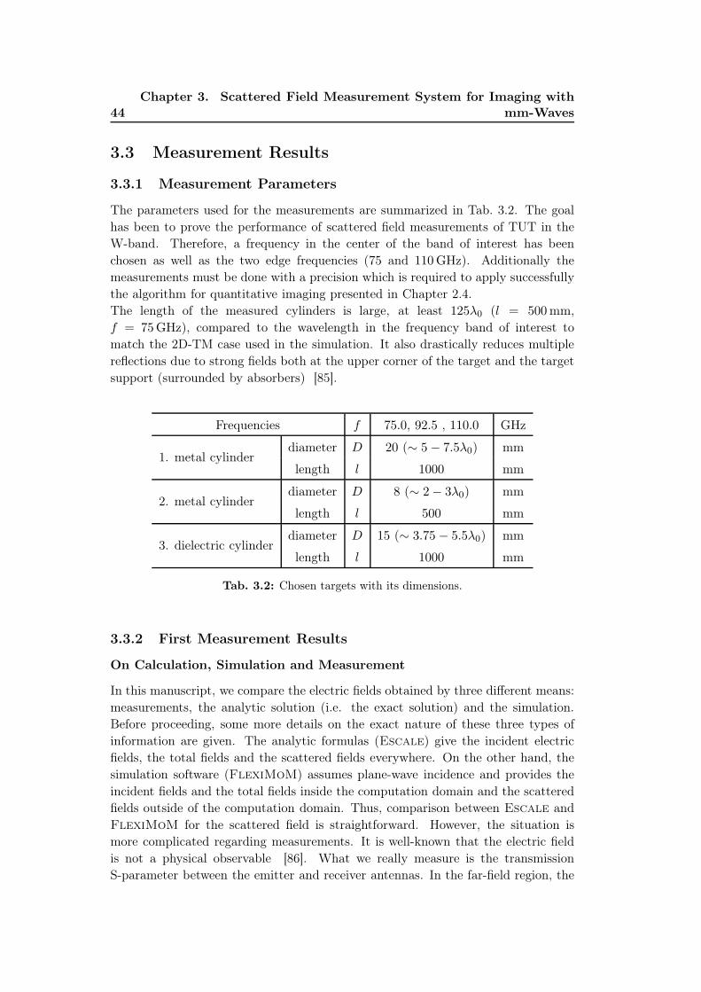
44Chapter 3. Scattered Field Measurement System for Imaging with
mm-Waves
3.3 Measurement Results
3.3.1 Measurement Parameters
The parameters used for the measurements are summarized in Tab. 3.2. The goalhas been to prove the performance of scattered field measurements of TUT in theW-band. Therefore, a frequency in the center of the band of interest has beenchosen as well as the two edge frequencies (75 and 110GHz). Additionally themeasurements must be done with a precision which is required to apply successfullythe algorithm for quantitative imaging presented in Chapter 2.4.The length of the measured cylinders is large, at least 125λ0 (l = 500mm,f = 75GHz), compared to the wavelength in the frequency band of interest tomatch the 2D-TM case used in the simulation. It also drastically reduces multiplereflections due to strong fields both at the upper corner of the target and the targetsupport (surrounded by absorbers) [85].
Frequencies f 75.0, 92.5 , 110.0 GHz
1. metal cylinderdiameter D 20 (∼ 5− 7.5λ0) mm
length l 1000 mm
2. metal cylinderdiameter D 8 (∼ 2− 3λ0) mm
length l 500 mm
3. dielectric cylinderdiameter D 15 (∼ 3.75 − 5.5λ0) mm
length l 1000 mm
Tab. 3.2: Chosen targets with its dimensions.
3.3.2 First Measurement Results
On Calculation, Simulation and Measurement
In this manuscript, we compare the electric fields obtained by three different means:measurements, the analytic solution (i.e. the exact solution) and the simulation.Before proceeding, some more details on the exact nature of these three types ofinformation are given. The analytic formulas (Escale) give the incident electricfields, the total fields and the scattered fields everywhere. On the other hand, thesimulation software (FlexiMoM) assumes plane-wave incidence and provides theincident fields and the total fields inside the computation domain and the scatteredfields outside of the computation domain. Thus, comparison between Escale andFlexiMoM for the scattered field is straightforward. However, the situation ismore complicated regarding measurements. It is well-known that the electric fieldis not a physical observable [86]. What we really measure is the transmissionS-parameter between the emitter and receiver antennas. In the far-field region, the

3.3. Measurement Results 45
Complex Antenna Factor (CAF), [87] is defined as the ratio between the complexelectric field incident on the antenna and the complex matched output voltage ofthe same antenna. In general, the CAF depends both on frequency and on angleof incidence. However, in our special case, the receiver “sees” the scatterer alwaysunder the same configuration, thus, the angle of incidence is constant and the CAF isonly frequency-dependent. This remark permits us to easily obtain the electric fieldsfrom the measurement of the S-parameters. S-parameters can be measured with thereceiver in linear magnitude and phase. S21 is proportional to the electrical field inthe presented system through the effective length on the antennas [88] because weare working in the far-field area. The scattered field is extracted from the subtractionof the total field (the field in the presence of the target, E(t)
meas.) and the incident
field (the field measured without any target, E(i)meas.):
E(s) = E(t)meas. −E(i)
meas.. (3.1)
This requires accurate amplitude and phase measurements. All the results in thismanuscript are shown as a function of the measurement angle φ (see Fig. 3.1 (bot-tom)) with φ = 180◦ corresponding to the forward scattering direction. As thetargets of interest are axially symmetrical, the multi-incidence/single-view measure-ment configuration can be equivalently considered as a single-incidence/multi-viewsetup. This second approach is used to obtain simulated (FlexiMoM) and an-alytical (Escale) data. In the theory described in Section 2.2, electric fields arecalculated on independent points in free space, that means the receivers are modeledas ideal isotropic antennas. In an experimental environment this condition can notbe fulfilled, as the results are influenced by the superposition of the radiation pat-terns of emitting and receiving antenna. For this reason the measured incident andtotal fields cannot be directly compared with numerical simulations. As a result,the amplitude of the incident field in the area close to the emitter (see Fig. 3.1) isbelow the noise-floor (see Fig. 3.4) for φ < 120◦ and φ > 240◦ here shown for theconfiguration with a standard gain horn as receiver and an open-ended waveguideas emitter. This limits the accuracy of the extracted scattered field because onlythe total field remains in this zone after the vectorial subtraction (see Fig. 3.5 andFig. 3.6 (top)). Therefore, the total field must have a significant higher level than themeasured incident field there, which is the case for the presented results (∼ 20 dB
above noise). With Fig. 3.4 one can estimate the dynamic of the measurements donewith this configuration to 35 dB.We obtain the measured scattered field after subtraction of the incident field fromthe total one. In order to compare measured and simulated scattered fields, we firstnormalize both of them with respect to their maximum amplitude (see Fig. 3.6).

46Chapter 3. Scattered Field Measurement System for Imaging with
mm-Waves
-90-80-70-60-50-40-30-20-10
0
60 120 180 240 300
Am
plitud
ein
dB
φ in degree
-4-3-2-101234
60 120 180 240 300
Pha
sein
rad
φ in degree
-600-500-400-300-200-100
0100
60 120 180 240 300
Unw
.ph
ase
inrad
φ in degree
Fig. 3.4: Measured incident field (raw measurements) for f = 92.5GHz in amplitude (top),
phase (middle) and unwrapped phase (bottom).
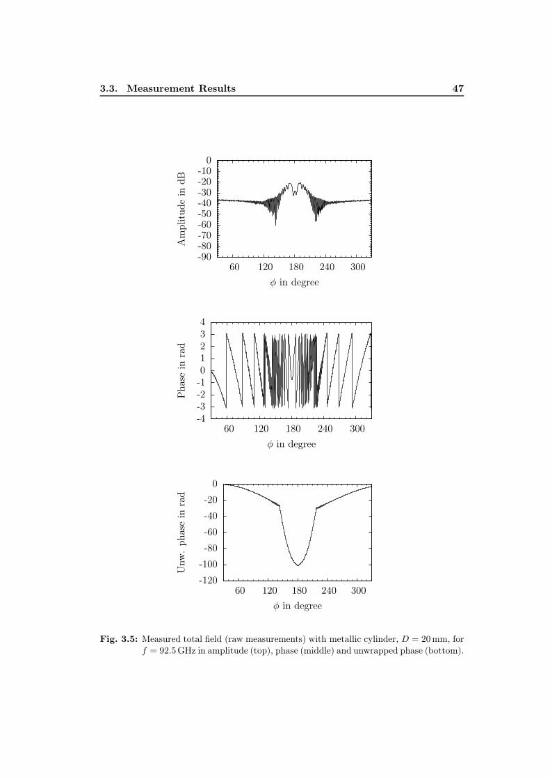
3.3. Measurement Results 47
-90-80-70-60-50-40-30-20-10
0
60 120 180 240 300
Am
plitud
ein
dB
φ in degree
-4-3-2-101234
60 120 180 240 300
Pha
sein
rad
φ in degree
-120
-100
-80
-60
-40
-20
0
60 120 180 240 300
Unw
.ph
ase
inrad
φ in degree
Fig. 3.5: Measured total field (raw measurements) with metallic cylinder, D = 20mm, for
f = 92.5GHz in amplitude (top), phase (middle) and unwrapped phase (bottom).

48Chapter 3. Scattered Field Measurement System for Imaging with
mm-Waves
-30
-20
-10
0
60 120 180 240 300
Nor
m.
ampl
itud
ein
dB
φ in degree
measured Escale
-4-3-2-101234
60 120 180 240 300
Pha
sein
rad
φ in degree
-45-40-35-30-25-20-15-10-50
60 120 180 240 300
Unw
.ph
ase
inrad
φ in degree
Fig. 3.6: Extracted scattered field (raw measurements) with metallic cylinder, D = 20mm,
for f = 92.5GHz in normalized amplitude (top), phase (middle) and unwrapped
phase (bottom).

3.3. Measurement Results 49
Reproducibility of Measurements
In order to verify the reproducibility of measurements, the incident field has beenmeasured twice and named with E(i)
1 and E(i)2 respectively. The difference is obtained
by subtracting the two measurements. This has been done with the standard-gainhorn used as emitter and receiver. The magnitude of this difference is less than−34 dB (see Fig. 3.7 (top)). Additional, the relative error is calculated see (3.2). Themaximal relative difference is 2% as shown in Fig. 3.7 (bottom). This demonstratesthat the measurements with the installed system are repeatable.
Relative difference =
∣∣∣E(i)1 − E
(i)2
∣∣∣(∣∣∣E(i)
1
∣∣∣+∣∣∣E(i)
2
∣∣∣)/2
(3.2)
-100-90-80-70-60-50-40-30-20-10
0
60 120 180 240 300
Diff
eren
cein
dB
φ in degree
0
0.5
1
1.5
2
60 120 180 240 300
Rel
ativ
edi
ffer
ence
in%
φ in degree
Fig. 3.7: Difference between measured incident fields (raw measurements) for
f = 92.5GHz (top) and relative difference (bottom). The configuration
contains a standard-gain horn as emitter and as receiver.

50Chapter 3. Scattered Field Measurement System for Imaging with
mm-Waves
Choice of Antennas
The choice of emitting and receiving antennas has to be made with respect to theSFMS constraints. Two open-ended waveguides and two standard gain horns withtheir four possible combinations as receiver and transmitter have been taken intoconsideration. The standard gain horn [89] has an aperture of 13 by 9mm2 andis 32.5mm long. An open-ended waveguide as emitting antenna provides on onehand a less directive radiation pattern which ensures a constant illumination ofthe targets. As a result, a malpositioning of the cylinder out of the center is lesscritical (see Fig. 3.6 and 3.10). On the other hand, more points of measurementare closer to the noise floor of the receiver module (−70 dBm) and therefore morenoised (see Fig. 3.4 (top)). This is enforced if the open-ended waveguide is also usedas receiver as shown in Fig. 3.10. This can be avoided by the use of a standard gainhorn. Then the received power level is enhanced because of the higher antenna gain(see Fig. 3.6). Its application as emitter in the same time provides a less constantillumination and increases the asymmetry due to an imprecision in positioning aspresented in Fig. 3.9. This problem is discussed more in detail in the next section.Therefore, the best results have been obtained by using the open-ended waveguideas emitting antenna and the standard gain horn as receiver. This is a trade-off inhaving an acceptable noise level and to illuminate the target with an almost constantfield strength in the target cross-section as plotted in Fig. 3.6. The open-endedwaveguide is used as emitter in combination with the standard-gain horn as receiverfor all measurements in the following. The three targets were fixed successively, andmeasurement cycles have been accomplished in the same manner for each frequencyand each cylinder to achieve the total field including the influence of the cylinder.The results are shown in Fig. 3.11 and Fig. 3.13. Afterwards the scattered field hasbeen extracted and is presented in Fig. 3.12 and Fig. 3.14 for the small metalliccylinder and the dielectric cylinder respectively.

3.3. Measurement Results 51
-30
-20
-10
0
60 120 180 240 300
Nor
m.
ampl
itud
ein
dB
φ in degree
measured Escale
-4-3-2-101234
60 120 180 240 300
Pha
sein
rad
φ in degree
-40-35-30-25-20-15-10-505
60 120 180 240 300
Unw
.ph
ase
inrad
φ in degree
Fig. 3.8: Extracted scattered field (raw measurements) with metallic cylinder, D = 20mm,
for f = 92.5GHz in normalized amplitude (top), phase (middle) and unwrapped
phase (bottom). The configuration contains an open-ended waveguide as receiver
and a standard-gain horn as emitter.

52Chapter 3. Scattered Field Measurement System for Imaging with
mm-Waves
-30
-20
-10
0
60 120 180 240 300
Nor
m.
ampl
itud
ein
dB
φ in degree
measured Escale
-4-3-2-101234
60 120 180 240 300
Pha
sein
rad
φ in degree
-55-50-45-40-35-30-25-20-15-10-50
60 120 180 240 300
Unw
.ph
ase
inrad
φ in degree
Fig. 3.9: Extracted scattered field (raw measurements) with metallic cylinder, D = 20mm,
for f = 92.5GHz in normalized amplitude (top), phase (middle) and unwrapped
phase (bottom). The configuration contains a standard-gain horn as receiver and
as emitter.

3.3. Measurement Results 53
-30
-20
-10
0
60 120 180 240 300
Nor
m.
ampl
itud
ein
dB
φ in degree
measured Escale
-4-3-2-101234
60 120 180 240 300
Pha
sein
rad
φ in degree
-45-40-35-30-25-20-15-10-50
60 120 180 240 300
Unw
.ph
ase
inrad
φ in degree
Fig. 3.10: Extracted scattered field (raw measurements) with metallic cylinder,
D = 20mm, for f = 92.5GHz in normalized amplitude (top), phase (middle)
and unwrapped phase (bottom). The configuration contains an open-ended
waveguide as receiver and as emitter.

54Chapter 3. Scattered Field Measurement System for Imaging with
mm-Waves
-90-80-70-60-50-40-30-20-10
0
60 120 180 240 300
Am
plitud
ein
dB
φ in degree
-4-3-2-101234
60 120 180 240 300
Pha
sein
rad
φ in degree
-140-120-100-80-60-40-20
0
60 120 180 240 300
Unw
.ph
ase
inrad
φ in degree
Fig. 3.11: Measured total field (raw measurements) with metallic cylinder, D = 8mm, for
f = 92.5GHz in amplitude (top), phase (middle) and unwrapped phase (bot-
tom).

3.3. Measurement Results 55
-30
-20
-10
0
60 120 180 240 300
Nor
m.
ampl
itud
ein
dB
φ in degree
measured Escale
-4-3-2-101234
60 120 180 240 300
Pha
sein
rad
φ in degree
-25
-20
-15
-10
-5
0
5
60 120 180 240 300
Unw
.ph
ase
inrad
φ in degree
Fig. 3.12: Extracted scattered field (raw measurements) with metallic cylinder,D = 8mm,
for f = 92.5GHz in normalized amplitude (top), phase (middle) and unwrapped
phase (bottom).

56Chapter 3. Scattered Field Measurement System for Imaging with
mm-Waves
-90-80-70-60-50-40-30-20-10
0
60 120 180 240 300
Am
plitud
ein
dB
φ in degree
-4-3-2-101234
60 120 180 240 300
Pha
sein
rad
φ in degree
-80-70-60-50-40-30-20-10
01020
60 120 180 240 300
Unw
.ph
ase
inrad
φ in degree
Fig. 3.13: Measured total field (raw measurements) with dielectric cylinder for
f = 92.5GHz in amplitude (top), phase (middle) and unwrapped phase (bot-
tom).

3.3. Measurement Results 57
-30
-20
-10
0
60 120 180 240 300
Nor
m.
ampl
itud
ein
dB
φ in degree
measured Escale
-4-3-2-101234
60 120 180 240 300
Pha
sein
rad
φ in degree
-18-16-14-12-10-8-6-4-2024
60 120 180 240 300
Unw
.ph
ase
inrad
φ in degree
Fig. 3.14: Extracted scattered field (raw measurements) with dielectric cylinder for
f = 92.5GHz in normalized amplitude (top), phase (middle) and unwrapped
phase (bottom). For the simulation with Escale a diameter of D = 15mm
and a relative permittivity of εr = 2.5 have been taken.

58Chapter 3. Scattered Field Measurement System for Imaging with
mm-Waves
Results for 75GHz and 110GHz are presented in the Annex C.Although the simulated and measured scattered fields are close to each other, onecan identify the following problems with respect to measurements:
• the amplitude calculated out of the measured values, apart from the mainlobe, as well as the phase of the scattered field, are degraded by noise,
• the secondary lobes are drastically degraded by noise,
• the measured phase, observed on its own, is not symmetric,
• measurements need to be properly normalized in order to take into accountthe difference between the incident powers in measurement and simulation.
Possible reasons for this are explained in the following section, and proposals for re-liable post-processing techniques in order to correct the measurements are disclosedand performed.
3.4 Analysis and Error Correction
As already mentioned in the previous section, the measured fields are degraded bynoise as well as the extracted scattered field. In general, noise is introduced bythe equipment itself and also by unavoidable reflections in the anechoic chamber.Moreover, additional noise, provoked by imprecision in the points of measurement,is going to be explained in detail and eliminated with digital filtering in the follow-ing. In addition, an asymmetry of the measured phase, caused by a mechanicalmisalignment, will be identified and corrected by post-processing. Furthermore,investigations are going to be done in the characterization of the complex relativepermittivity of the dielectric cylinder as this is mandatory to compare its simulatedand measured fields for the frequency of interest.
3.4.1 Characterization of Dielectric Targets
Before comparing measured scattered fields with simulated one, one must exactlycharacterize the TUT in order to provide comparable synthetic data. The usedacrylic cylinder was supposed to provide the following characteristics: a diameter Dof 15mm (given by the manufacturer), an εr = 2.5 with no losses (corresponding toacrylic). No reliable values have been found in the literature for the dielectric con-stant of the acrylic in the W-band. In the past, dielectric scatterers of PolymethylMethacrylate (PMMA) have been often used as reference target because these plas-tics are remarkably consistent in their refractive index. Furthermore, there is indeedno measurable frequency dependence [90].

3.4. Analysis and Error Correction 59
Differences in Diameter
The first studied parameter which influences the scattered fields is the diameter D.Its actual value has been measured to D = 15.4mm. The previous taken value,provided by the manufacturer, has been D = 15mm. The scattered fields have beensimulated with Escale for both diameters and are compared in Fig. 3.15. Thedifference of 400µm in diameter provokes minor discrepancies in amplitude in thebackscattered region. On the contrary, not negligible differences occur in this regionin phase (see Fig. 3.15 (right)).
-60
-50
-40
-30
-20
-10
0
180 240 300 360
Am
plitud
ein
dB
φ in degree
D = 15.4mmD = 15mm
-4-3-2-101234
180 240 300 360
Pha
sein
rad
φ in degree
Fig. 3.15: Simulated scattered field (Escale) for different diameters for f = 92.5GHz in
amplitude (left) and phase (right).
Differences in the Complex Permittivity
In order to study the influence of different σ and εr of our target investigations havebeen done in simulation [122]. To estimate experimentally the actual permittivityand conductivity of a sample, made of the same acrylic as the measured cylinder,a characterization has been done with a quasi-optical measurement setup as usedin [91]. The values of εr and tan δ could be measured for two resonance frequenciesas shown in Tab. 3.3. Simulations have been investigated with these parametersand are shown in Fig. 3.16. For both cases no notable changes can be seen for theamplitude. Minor differences in the phase occur.
Resonant frequency εr tan δ
69.13GHz 2.44 0.0077
102.4GHz 2.49 0.0082
Tab. 3.3: Measured values for characterized dielectric samples.
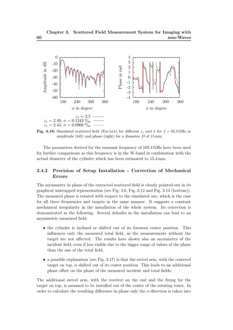
60Chapter 3. Scattered Field Measurement System for Imaging with
mm-Waves
-60
-50
-40
-30
-20
-10
0
180 240 300 360
Am
plitud
ein
dB
φ in degree
εr = 2.5εr = 2.49, σ = 0.1243 S/mεr = 2.44, σ = 0.0966 S/m
-4-3-2-101234
180 240 300 360
Pha
sein
rad
φ in degree
Fig. 3.16: Simulated scattered field (Escale) for different εr and σ for f = 92.5GHz in
amplitude (left) and phase (right) for a diameter D of 15mm.
The parameters derived for the resonant frequency of 102.4GHz have been usedfor further comparisons as this frequency is in the W-band in combination with theactual diameter of the cylinder which has been estimated to 15.4mm.
3.4.2 Precision of Setup Installation - Correction of MechanicalErrors
The asymmetry in phase of the extracted scattered field is clearly pointed-out in itsgraphical unwrapped representation (see Fig. 3.6, Fig. 3.12 and Fig. 3.14 (bottom)).The measured phase is rotated with respect to the simulated one, which is the casefor all three frequencies and targets in the same manner. It suggests a constantmechanical irregularity in the installation of the whole system. Its correction isdemonstrated in the following. Several defaults in the installation can lead to anasymmetric measured field:
• the cylinder is inclined or shifted out of its foreseen center position. Thisinfluences only the measured total field, as the measurements without thetarget are not affected. The results have shown also an asymmetry of theincident field, even if less visible due to the bigger range of values of the phasethan the one of the total field,
• a possible explanation (see Fig. 3.17) is that the swivel arm, with the centeredtarget on top, is shifted out of its center position. This leads to an additionalphase offset on the phase of the measured incident and total fields.
The additional swivel arm, with the receiver on the end and the fixing for thetarget on top, is assumed to be installed out of the center of the rotating tower. Inorder to calculate the resulting difference in phase only the x-direction is taken into

3.4. Analysis and Error Correction 61
ideal centershifted center
x
y
incident plane wavex(φ′)
x(φ′)βφ
φ
rcircle
fix
shifted swivel arm with receiver
rotating tower
start position
stop position
φ′
Fig. 3.17: Planned symmetric installation of the swivel arm with receiver and target on
top and its shifted mounting.
account as it is parallel to the propagation direction of the incident plane wave. Onone hand, this comes along with an additional unsymmetrical part in phase to theincident field, as the receiver does not turn on an ideal circle any more. On the otherhand, an additional phase is added to the total field. This is also not symmetric asfunction of φ, as the movement of the target describes a circle instead of turningon its axis of symmetry (Fig. 3.17). The arm is shifted by rcircle from the center ofthe tower and by β with respect to φ, where φ describes the position of the rotatingtower φ ∈ [30◦ · · · 330◦]. The actual accomplished position of the swivel arm is:
φ′ = φ+ β. (3.3)
The additional length as function of φ can be calculated as following and isreduced by rcircle in order to obtain only the difference in length x′ due to themismatch:
x(φ′) = rcircle cos(φ′) (3.4)
x′(φ′) = x(φ′)− rcircle = rcircle[1− cos(φ′)
]. (3.5)
Finally, this error in distance can be expressed with the equivalent phase Φ:
Φ(φ) = −(2πx′)
λ0. (3.6)
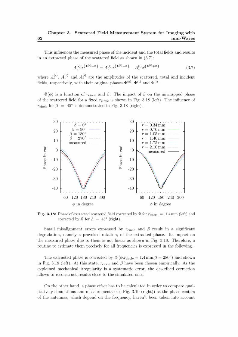
62Chapter 3. Scattered Field Measurement System for Imaging with
mm-Waves
This influences the measured phase of the incident and the total fields and resultsin an extracted phase of the scattered field as shown in (3.7):
A(s)z ej(Φ
(s)+Φ) = A(t)z ej(Φ
(t)+Φ) −A(i)z ej(Φ
(i)+Φ) (3.7)
where A(s)z , A(t)
z and A(i)z are the amplitudes of the scattered, total and incident
fields, respectively, with their original phases Φ(s), Φ(t) and Φ(i).
Φ(φ) is a function of rcircle and β. The impact of β on the unwrapped phaseof the scattered field for a fixed rcircle is shown in Fig. 3.18 (left). The influence ofrcircle for β = 45◦ is demonstrated in Fig. 3.18 (right).
-40
-30
-20
-10
0
10
20
30
60 120 180 240 300
Pha
sein
rad
φ in degree
β = 0◦
β = 90◦
β = 180◦
β = 270◦
measured
-40
-30
-20
-10
0
10
20
30
60 120 180 240 300
Pha
sein
rad
φ in degree
r = 0.34mmr = 0.70mmr = 1.05mmr = 1.40mmr = 1.75mmr = 2.10mm
measured
Fig. 3.18: Phase of extracted scattered field corrected by Φ for rcircle = 1.4mm (left) and
corrected by Φ for β = 45◦ (right).
Small misalignment errors expressed by rcircle and β result in a significantdegradation, namely a provoked rotation, of the extracted phase. Its impact onthe measured phase due to them is not linear as shown in Fig. 3.18. Therefore, aroutine to estimate them precisely for all frequencies is expressed in the following.
The extracted phase is corrected by Φ (φ,rcircle = 1.4mm,β = 280◦) and shownin Fig. 3.19 (left). At this state, rcircle and β have been chosen empirically. As theexplained mechanical irregularity is a systematic error, the described correctionallows to reconstruct results close to the simulated ones.
On the other hand, a phase offset has to be calculated in order to compare qual-itatively simulations and measurements (see Fig. 3.19 (right)) as the phase centersof the antennas, which depend on the frequency, haven’t been taken into account

3.4. Analysis and Error Correction 63
yet in the simulation. The estimation of the real distance between the antennas andthe target would still remain a challenging task and can be estimated only based ona more complex and more accurate installation than the actual one. Therefore, thedifference between simulated and extracted phase of the scattered field is calculatedas averaged offset in a zone at φ = 180◦ ± 5◦ and subtracted from the latter one(3.8):
averaged offset =φ=185◦∑
φ=175◦
Φ(s)measured(φ)− Φ(φ)− Φ
(s)simulated(φ)
number of points. (3.8)
-40
-30
-20
-10
0
10
20
30
60 120 180 240 300
Pha
sein
rad
φ in degree
measuredEscale
corrected
-40
-30
-20
-10
0
10
20
30
60 120 180 240 300
Pha
sein
rad
φ in degree
corr., offsetEscale
Fig. 3.19: Phase of extracted scattered field corrected by
Φ (φ,rcircle = 1.4mm,β = 280◦) (left) and phase of extracted scattered
field corrected by Φ (φ,rcircle = 1.4mm,β = 280◦,offset = −1.45 rad) (right).
After the phase correction, very good agreement is obtained between thesimulation results and the measured ones.
The actual imprecision due to rcircle and β couldn’t be measured because of tworeasons:
• The measurements were done in a limited frame of time as the anechoic cham-ber is used by different research teams. As a consequence the system had beenremoved before the measurements were fully analyzed.
• The presented shift (rcircle ∼ 1.4mm) is too small to be detected and surveyedwith conventional tools with a sufficient precision. This magnitude of mechan-ical errors have been less critical for installations used at lower frequencies upto now in the laboratory.

64Chapter 3. Scattered Field Measurement System for Imaging with
mm-Waves
Therefore, a process has been developed to improve the accuracy of rcircle and β,explained below: in order to identify the error, which corresponds most to the usedsetup, an optimization is conducted. For this purposes the built-in function ofOctave fmins has been used. The cost function is calculated as:
C =1
N
N∑
n=1
∣∣∣∣(Φ
(s)measured(n)− Φ(rcircle, β, n)− GO
)− Φ
(s)simulation(n)
∣∣∣∣
where N is the number of measured points and Φ(s)measured(n) and Φ
(s)simulation(n) are
the extracted and simulated unwrapped phases of the measured and simulated scat-tered fields, respectively. The global offset (GO) is a scalar value. It is used as asimple phase normalization of the optimization process. As initial guess for the theoptimization the averaged offset (3.8) is taken therefore. The optimization functionfinds the minimum of the cost function with the variables rcircle, β and GO. Bydefault, the method used is the Nelder & Mead Simplex algorithm [92]. Investiga-tions have been done in order to study the number of points of measurements takinginto account for the optimization. Therefore, the metallic cylinder of D = 20mm
is taken as reference and future calibration target. The variables rcircle and β havebeen calculated with the described optimization routine as function of the numberof points and the frequency. Thus, equispaced points have been chosen out of the1501 available measured points (see Fig. 3.20).

3.4. Analysis and Error Correction 65
0.2
0.4
0.6
0.8
1
1.2
1.4
1.6
251301376
501
751
1501
r circl
ein
mm
Number of points
75.0GHz92.5GHz
110.0 GHz
100120140160180200220240260280300320
251301376
501
751
1501
βin
degr
ee
Number of points
Fig. 3.20: Calculated coefficients after optimization; radius rcircle (top) and direc-
tion β (bottom).

66Chapter 3. Scattered Field Measurement System for Imaging with
mm-Waves
The results show that almost constant calibration coefficients rcircle and β arefound over the three frequencies and over the number of points. Results for 75GHz
and 1501 points have to be excluded as there is one point of the phase whichdegrades drastically the unwrapped phase. As the cost-function is less for 751
and 1501 points, these results have been averaged over the three frequencies. Thislead to a rcircle = 1.51mm and β = 290.3◦. These values have been supposed toestimate best the shift of the installed system and have been used as calibrationcoefficients in the following section to calibrate the measurement results. Theobtained calibrated measured scattered field is called E
(s)cal..
3.4.3 Match Experimental Setup with Simulation - Complex Nor-malization
After the presented calibration a normalization [19] of the amplitude and the phasecan be done. In order to match the experimental setup with the direct problem, anormalization on amplitude and phase has to be done on the data, by comparingthem with synthetic (analytic solution) ones, matching more or less the targets.The complex normalization factor γ can be calculated, in case of known objects,as function of the measured scattered field and the simulated field [35] taking intoaccount the receivers m = 1, · · · ,M:
γ =
∑Mm=1
⟨(E
(s)exact
)m,(E
(s)cal.
)m
⟩
∑Mm=1
∥∥∥(E
(s)cal.
)
m
∥∥∥2 (3.9)
with the following definition of the discrete scalar product and the quadratic normfor vectors with complex entries:
〈v1, v2〉 =M∑
m=1
v1mv2m
‖v1‖2 = 〈v1, v1〉 .
Finally the measured scattered field calibrated and normalized(E
(s)cal.,norm.
)is
obtained.
3.4. Analysis and Error Correction 67
3.4.4 Noise Sources - Filtering
Per definition, the measured electric fields include systematic and random errors.The first one are repeatable, their origin can be identified and quantified, they areknown as systematic errors. In other words they can be corrected by the calibrationwith the presented calibration coefficients (rcircle, β).
Signal-to-Noise Ratio Definition
As for any experimental study, defining a signal-to-noise ratio is an important stepto analyze qualitatively the obtained results.
One can define the measurement error (e). The noise affecting the data is re-lated to the mm-wave module and the receiver (noise floor, thermal drift), parasitereflections in the cables of the measurement system, unavoidable reflections in theanechoic chamber, misalignment errors (positioning of emitter, target and receiver)and random errors (deviation in measurement points shown in the following for ex-ample). After the calibration the remaining errors are due to random phenomenaand one can define the SNR [93] based on the error e to evaluate the quality of theresults at each frequency as following:
e =
⟨E
(s)cal.,norm. − E
(s)exact, E
(s)cal.,norm. − E
(s)exact
⟩
⟨E
(s)exact, E
(s)exact
⟩ (3.10)
SNR
∣∣∣∣dB
=− 10 log (e) (3.11)
where E(s)cal.,norm. are the scattered fields, calibrated and normalized, issued from
measurements and E(s)exact the exact fields. This reference signal is calculated with
the analytic solution (Escale) because it is the exact solution as no numericalnoise is introduced as it would be the case for the simulation with FlexiMoM.
Two main sources of noise have been identified: on one hand, measurements arenoisy due to the noise introduced by the equipment itself used for our measurements.On the other hand, the mechanical configuration comes into play: the scattered fieldsare obtained after subtraction of the incident and total fields. That means that twomeasurement cycles are mandatory to obtain one set of measurements correspondingto the scattered field. Additional noise occurs if the measurement points are not thesame within these two measurement cycles.
Noise by Shift in Measurement Points
To perform the measurements, the highest precision possible for the positioning ofthe step engine, 0.05◦ has been chosen by software. The log files (see Tab. 3.4 fortwo measurements) show the actual deviation in approached and reached position,of the step motor for every cycle of measurements. In order to take into account this
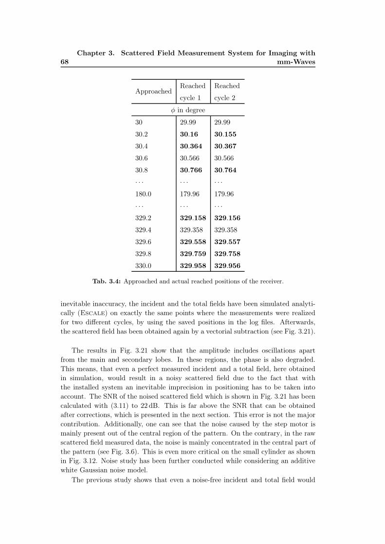
68Chapter 3. Scattered Field Measurement System for Imaging with
mm-Waves
ApproachedReached Reached
cycle 1 cycle 2
φ in degree
30 29.99 29.99
30.2 30.16 30.155
30.4 30.364 30.367
30.6 30.566 30.566
30.8 30.766 30.764
· · · · · · · · ·180.0 179.96 179.96
· · · · · · · · ·329.2 329.158 329.156
329.4 329.358 329.358
329.6 329.558 329.557
329.8 329.759 329.758
330.0 329.958 329.956
Tab. 3.4: Approached and actual reached positions of the receiver.
inevitable inaccuracy, the incident and the total fields have been simulated analyti-cally (Escale) on exactly the same points where the measurements were realizedfor two different cycles, by using the saved positions in the log files. Afterwards,the scattered field has been obtained again by a vectorial subtraction (see Fig. 3.21).
The results in Fig. 3.21 show that the amplitude includes oscillations apartfrom the main and secondary lobes. In these regions, the phase is also degraded.This means, that even a perfect measured incident and a total field, here obtainedin simulation, would result in a noisy scattered field due to the fact that withthe installed system an inevitable imprecision in positioning has to be taken intoaccount. The SNR of the noised scattered field which is shown in Fig. 3.21 has beencalculated with (3.11) to 22 dB. This is far above the SNR that can be obtainedafter corrections, which is presented in the next section. This error is not the majorcontribution. Additionally, one can see that the noise caused by the step motor ismainly present out of the central region of the pattern. On the contrary, in the rawscattered field measured data, the noise is mainly concentrated in the central part ofthe pattern (see Fig. 3.6). This is even more critical on the small cylinder as shownin Fig. 3.12. Noise study has been further conducted while considering an additivewhite Gaussian noise model.
The previous study shows that even a noise-free incident and total field would

3.4. Analysis and Error Correction 69
-30
-20
-10
0
60 120 180 240 300
Am
plitud
ein
dB
φ in degree
noisyexact -4
-3-2-101234
60 120 180 240 300
Pha
sein
rad
φ in degree
Fig. 3.21: Simulated scattered field (Escale) on points of the step motor, where mea-
surements have been provided, D = 2 cm, f = 92.5GHz, in amplitude (left)
and phase (right).
result in a noised scattered field due to the fact that the measurements can’t beperformed on exactly the same points as foreseen. Even a marginal deviation inposition of the receiver, where the measurements are effected, leads to a noisy scat-tered field. To overcome this problem, a filtering has been applied directly on thescattered fields.
Additional White Gaussian Noise
In order to model the noise behavior of the equipment by itself in general, anAWGN [67] has been added to the simulations. It might not be totally accurate fornoise modeling of the measurement system but still provides a useful model for per-formance estimations. Fig. 3.22 shows the results of the large metallic cylinder for aSNR of 10 dB which corresponds to the value after calibration of the measured scat-tered field. As expected the AWGN shows a noise distribution that impacts all theradiation pattern over φ on the contrary to the noise introduced by the imprecisionof positioning of the step motor. This model will be used for further investigationson the filtering.
Noise by Superposition of Fields
On one hand, the results have shown that the imprecision in the approach of themeasuring points influences marginally the scattered field outside the main and thesecondary lobes. It is not the main cause for the noise in the scattered fields. Onthe other hand, an AWGN degrades equally the whole pattern of the scattered field.The scattered fields extracted from measurements are locally more influenced bynoise in the zone of the main and secondary lobes (see Fig. 3.6). The reason for thisis demonstrated in Fig. 3.23 by super-positioning of the measured incident and totalfields: in the region where the incident and the total fields are in the same order

70Chapter 3. Scattered Field Measurement System for Imaging with
mm-Waves
-30
-20
-10
0
60 120 180 240 300
Am
plitud
ein
dB
φ in degree
noisyexact
-4-3-2-101234
60 120 180 240 300
Pha
sein
rad
φ in degree
Fig. 3.22: Simulated extracted scattered field (Escale) with AWGN (SNR=10 dB),
D = 2 cm, f = 92.5GHz, in amplitude (left) and phase (right).
of magnitude the measurement errors are more contributing to the overall noiselevel of the extracted scattered field. One can retrieve that the noise distributionof the extracted scattered fields dominates in the regions where the total and theincident fields are close in values. For the metallic cylinders this zone of strongnoise contribution influences the main and secondary lobes. The scattered fieldextracted from measurements of the dielectric cylinder shows that the zone alsodegrades more side lobes where the measured total field has the same magnitude asthe incident field. For this reason, almost the whole measured area of the scatteredfield is degraded by noise. Further investigations on noise modeling are foreseenas following: to model precisely the actual noise distribution of the measurementsystem a comparison of the magnitudes of the incident and the total fields will bedone. Depending whether the magnitudes of the two fields are in the same order,AWGN based on different given values for SNR is calculated and determines theadditive noise to the simulated scattered fields.
The noise introduced by the step motor and by the equipment itself can bereduced by applying a low-pass filter on the extracted scattered fields. This is goingto be explained in the next section.
Ideal Filtering Based on Measurements
In order to suppress noise, a filtering, that does not require a-priori knowledge ofthe target, has been developed. It is important, because the final application ofinterest is quantitative imaging with unknown targets under test. Therefore, thefollowing filter process is applied: the scattered field as a function of the variableφ is transformed into the spectral domain with a Fourier transformation. Filteringis done with a multiplication by a rectangular window which has the width of thecut-off frequency (in 1/degree) as demonstrated exemplary in Fig. 3.24.
In order to obtain the best SNR, which can be obtained with filtering, the fol-

3.4. Analysis and Error Correction 71
-90-80-70-60-50-40-30-20-10
0
60 120 180 240 300
Am
plitud
ein
dB
φ in degree
total fieldincident field
Fig. 3.23: Amplitude of the measured total and incident fields (raw measurements) for the
metallic cylinder, D = 2 cm, f = 92.5GHz.
-60
-50
-40
-30
-20
-10
0
10
20
0 0.5 1 1.5 2 2.5
Mag
nitu
dein
dB
Frequency in 1/degree
variable cut-off frequency
Fig. 3.24: The scattered field of the metallic cylinder with a diameter of D = 20mm for
f = 92.5GHz as a function of the variable φ transformed into the spectral do-
main.

72Chapter 3. Scattered Field Measurement System for Imaging with
mm-Waves
lowing investigations have been done: the filter frequency has been decreased pro-gressively and the corresponding SNR value calculated; so far with the knowledgeof the target, the two metallic cylinders. The SNR as function of the cut-off fre-quency is shown in Fig. 3.25 (left) for the large cylinder (top) and the small cylinder(bottom). The maximal SNR reachable by the explained filtering depends on theexact knowledge of the cut-off frequency which has to be chosen. This frequencydepends on the TUT and the frequency of operation. For this cut-off frequency themaximum SNR is nearly constant over the measurement frequency, 15.81 dB for thelarge cylinder and 10.7 dB for the small cylinder. The results show that the bestSNR as function over the frequency comes with different losses due to the filtering(see Fig. 3.25 (right)). The signal losses are defined as the difference between thepower of the scattered field before and after filtering. Filtering relying on a criterionbased on a constant value of losses for all frequencies would result in a final SNR farbelow the best SNR achievable by filtering depending on the frequency of operationand target. The best SNR due to filtering is shown in Tab. 3.5. The two cases for751 and 1501 points of calibrated and normalized results have been calculated.
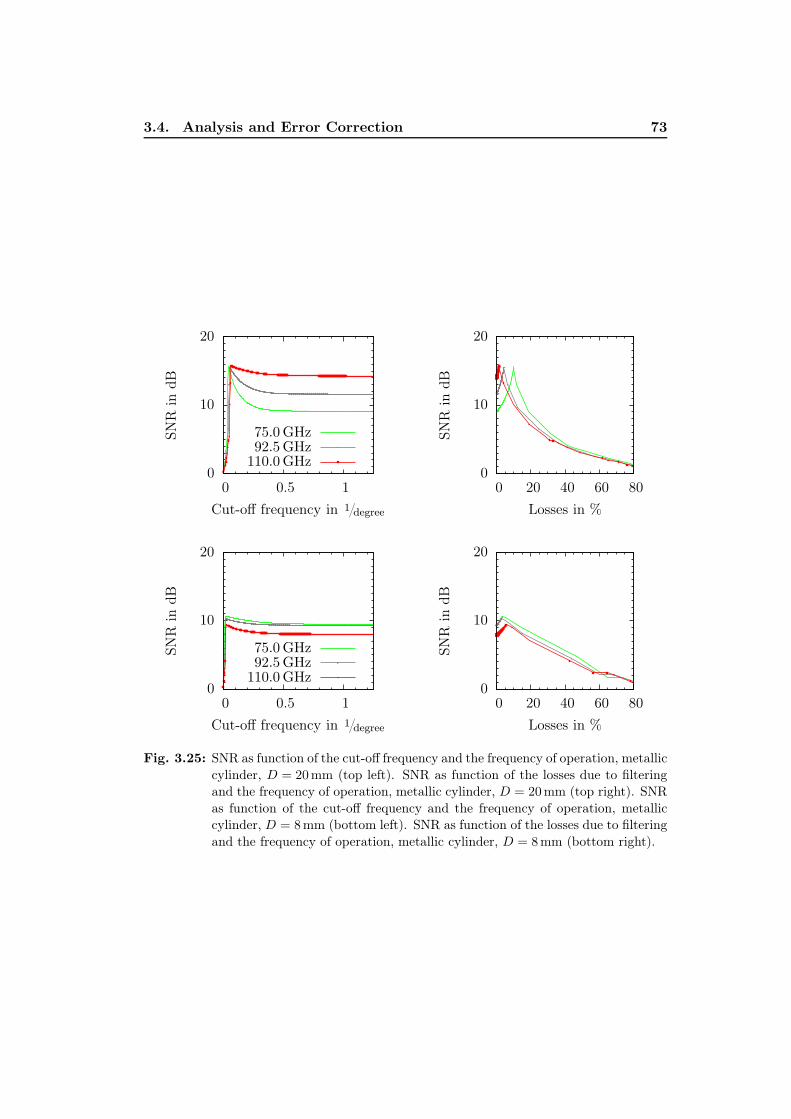
3.4. Analysis and Error Correction 73
0
10
20
0 0.5 1
SNR
indB
Cut-off frequency in 1/degree
75.0GHz92.5GHz110.0GHz
0
10
20
0 20 40 60 80
SNR
indB
Losses in %
0
10
20
0 0.5 1
SNR
indB
Cut-off frequency in 1/degree
75.0GHz92.5GHz110.0GHz
0
10
20
0 20 40 60 80
SNR
indB
Losses in %
Fig. 3.25: SNR as function of the cut-off frequency and the frequency of operation, metallic
cylinder, D = 20mm (top left). SNR as function of the losses due to filtering
and the frequency of operation, metallic cylinder, D = 20mm (top right). SNR
as function of the cut-off frequency and the frequency of operation, metallic
cylinder, D = 8mm (bottom left). SNR as function of the losses due to filtering
and the frequency of operation, metallic cylinder, D = 8mm (bottom right).

74
Chapte
r3.
Scatte
red
Fie
ldM
easu
rem
ent
Syste
mfo
rIm
agin
gw
ithm
m-W
aves
751 points 1501 points
SNR - max Slope detection SNR - max Slope detection
f SNR fc fc SNR SNR fc fc SNR
in in in in in in in in in
GHz dB 1/degree 1/degree dB dB 1/degree 1/degree dB
Metallic cylinder 75.0 15.64 0.047 0.043 15.31 15.67 0.047 0.043 15.32
D = 20mm92.5 15.46 0.057 0.053 14.97 15.46 0.057 0.053 15.00
110.0 15.81 0.067 0.067 15.74 15.81 0.070 0.067 15.75
75.0 10.64 0.020 0.020 10.64 10.70 0.020 0.020 10.70
D = 8mm92.5 10.36 0.023 0.023 10.36 10.34 0.023 0.023 10.34
110.0 9.40 0.027 0.030 9.33 9.44 0.027 0.030 9.37
Dielectric cylinder 75.0 5.65 0.033 0.037 5.55 5.67 0.033 0.037 5.56
D = 15mm92.5 6.03 0.043 0.047 5.97 6.06 0.043 0.047 6.00
110.0 5.54 0.057 0.053 5.54 5.53 0.057 0.053 5.53
Tab. 3.5: The maximal SNR achievable with filtering and its cut-off frequency compared with the cut-off frequency obtained by slope detection
(100 percent degree) and its SNR for 751 and 1501 points of measurements.

3.4. Analysis and Error Correction 75
The SNR based on (3.11) can only be calculated if the TUT is known, becauseso far the calibration and the SNR calculation have to be done with the syntheticdata for the known target. Other calibration schemes could be used to overcome thisproblem by taking a known scattered field by a reference target for calibration [72].Anyway the qualitative estimation of the SNR without synthetic data is a challeng-ing task especially if this value depends on the TUT. In order to get the optimalcut-off frequency of the filter, only based on measured data, the following procedurehas been used: the losses due to filtering as function of the cut-off frequency in thespectral domain have been calculated (see Fig. 3.26). For this, the cut-off frequencyis decreased progressively in order to get the signal losses as function of the cut-offfrequency. Indeed spectral domain of measurements has three regions:
• region 1: from 0 to a first value of the spectral variable (s1) the slope is veryhigh,
• region 2: from s1 to s2: a smaller slope,
• region 3: above s2 an almost flat curve.
The region 2 does not exist in the simulation as the results are free of noise. Onecan see that the value s1 is the same in the simulation and the measurement foreach frequency respectively.
Then the slope of this function can be directly calculated. Once the losses raisedrastically the real spectrum of the scattered field itself is filtered. In this way, theoptimal cut-off frequency of the filter can be found with a slope detection (frequencycorresponding to s1). In Fig. 3.27 the slope of the losses due to filtering based on themeasurement and on the simulated scattered field noised with a white Gaussian noise(SNR=5 dB) are compared. This works well for the scattered field measurementsof all targets and all frequencies (see Tab. 3.5). The only visible difference is onefrequency step between the calculated cut-off frequency found with the maximalSNR and the presented approach with the slope detection. The frequency resolutionin the spectral domain is 1/300◦.
In order to prove the function of the presented approach in general, simulationshave been investigated on asymmetric targets. Two objects of interest frommm-wave radar applications have been chosen. That is a thin metallic plate, usedas target of interest in FOD detection and a power line section, used as target ofinterest in collision avoidance radar for helicopters. The ideal simulated scatteredfields were noised with AWGN up to a SNR of 5 dB. Simulations were conductedwith FlexiMoM as no analytical model exists at least for the power line. Goingback to the filtering and applying the presented method, we found out that it is stillaccurate for asymmetric objects under AWGN. The results are shown in Fig. 3.28and Fig. 3.30.
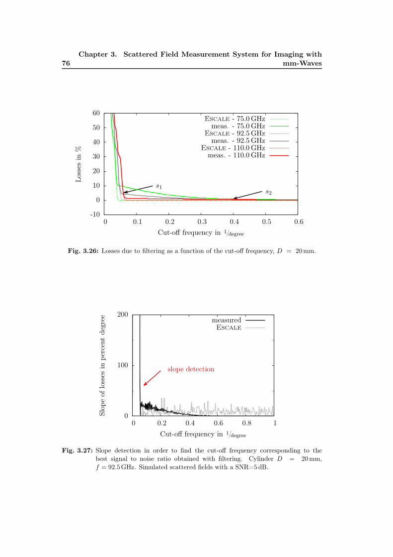
76Chapter 3. Scattered Field Measurement System for Imaging with
mm-Waves
-10
0
10
20
30
40
50
60
0 0.1 0.2 0.3 0.4 0.5 0.6
Los
ses
in%
Cut-off frequency in 1/degree
s1s2
Escale - 75.0GHzmeas. - 75.0GHz
Escale - 92.5GHzmeas. - 92.5GHz
Escale - 110.0 GHzmeas. - 110.0 GHz
Fig. 3.26: Losses due to filtering as a function of the cut-off frequency, D = 20mm.
0
100
200
0 0.2 0.4 0.6 0.8 1
Slop
eof
loss
esin
per
cent
degr
ee
Cut-off frequency in 1/degree
slope detection
measuredEscale
Fig. 3.27: Slope detection in order to find the cut-off frequency corresponding to the
best signal to noise ratio obtained with filtering. Cylinder D = 20mm,
f = 92.5GHz. Simulated scattered fields with a SNR=5 dB.

3.4. Analysis and Error Correction 77
The presented approach has been verified on measured data for three differentsymmetric targets and three frequencies. The approach is verified with irregularobjects as they are of particular interest for several applications which aim to detectobjects like rectangular targets or targets with special cross sections as shown in thefollowing.
Verification of Filtering - Metal Plate A metal plate (100mm × 5mm), anobject which is difficult to detect with actual radar systems on a runway of anairport, has been investigated. Its scattered fields have been calculated on 3600
equispaced points for a frequency of 100GHz for an angle of incidence of 45◦. Thedistance between the receivers and the center of the plate has been chosen to 300mm.The plate is considered to be infinite in z-direction to fulfill the 2D-TM case forsimulation purposes. An AWGN has been added to get a SNR of 5 dB to havean unfavorable case in measurement (see Fig. 3.28 (left)). The results have beenfiltered (see Fig. 3.28 (right)) with the presented approach which leads to a cut-offfrequency of 0.256 1/degree with a final SNR of 15.42 dB. This is very close to themaximal SNR of 16.95 dB with its cut-off frequency of 0.294 1/degree.
-50-40-30-20-10
01020
0 60 120 180 240 300 360
Am
plitud
ein
dB
φ in degree
noisyFlexiMoM
-50-40-30-20-10
01020
0 60 120 180 240 300 360
Am
plitud
ein
dB
φ in degree
FlexiMoMfiltered
Fig. 3.28: The scattered field of the thin metallic plate under 45◦ incidence (size of the
plate is 100mm× 5mm) before filtering (left) and after filtering (right).
Verification of Filtering - Cable Section A cable section (see description ofdimensions in Fig. 3.29), has been simulated with ρ1 = 8.5mm and ρ2 = 5mm.Its scattered fields have been calculated on 3600 equispaced points for a frequencyof 100GHz for an angle of incidence of 180◦ in a distance of 300mm. An AWGNhas been added to get a SNR of 5 dB to have an unfavorable case in measurement(see Fig. 3.30 (left)). The results have been filtered (see Fig. 3.30 (right)) with thepresented approach which leads to a cut-off frequency of 0.108 1/degree with a finalSNR of 20.87 dB. This is very close to the maximal SNR of 21.05 dB with its cut-offfrequency of 0.094 1/degree.
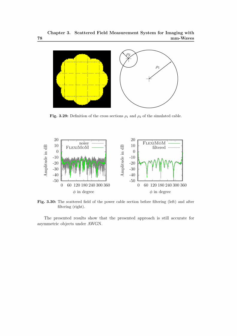
78Chapter 3. Scattered Field Measurement System for Imaging with
mm-Waves
ρ1
ρ2
Fig. 3.29: Definition of the cross sections ρ1 and ρ2 of the simulated cable.
-50-40-30-20-10
01020
0 60 120 180 240 300 360
Am
plitud
ein
dB
φ in degree
noisyFlexiMoM
-50-40-30-20-10
01020
0 60 120 180 240 300 360
Am
plitud
ein
dB
φ in degree
FlexiMoMfiltered
Fig. 3.30: The scattered field of the power cable section before filtering (left) and after
filtering (right).
The presented results show that the presented approach is still accurate forasymmetric objects under AWGN.
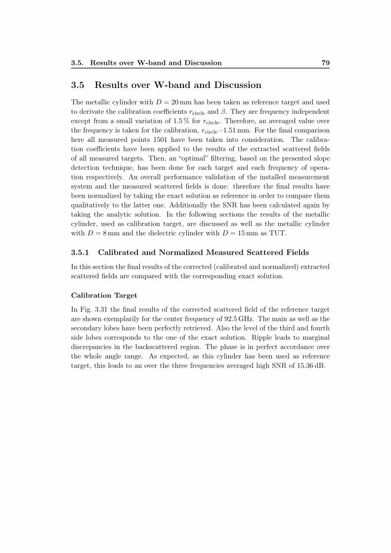
3.5. Results over W-band and Discussion 79
3.5 Results over W-band and Discussion
The metallic cylinder with D = 20mm has been taken as reference target and usedto derivate the calibration coefficients rcircle and β. They are frequency independentexcept from a small variation of 1.5% for rcircle. Therefore, an averaged value overthe frequency is taken for the calibration, rcircle=1.51mm. For the final comparisonhere all measured points 1501 have been taken into consideration. The calibra-tion coefficients have been applied to the results of the extracted scattered fieldsof all measured targets. Then, an “optimal” filtering, based on the presented slopedetection technique, has been done for each target and each frequency of opera-tion respectively. An overall performance validation of the installed measurementsystem and the measured scattered fields is done: therefore the final results havebeen normalized by taking the exact solution as reference in order to compare themqualitatively to the latter one. Additionally the SNR has been calculated again bytaking the analytic solution. In the following sections the results of the metalliccylinder, used as calibration target, are discussed as well as the metallic cylinderwith D = 8mm and the dielectric cylinder with D = 15mm as TUT.
3.5.1 Calibrated and Normalized Measured Scattered Fields
In this section the final results of the corrected (calibrated and normalized) extractedscattered fields are compared with the corresponding exact solution.
Calibration Target
In Fig. 3.31 the final results of the corrected scattered field of the reference targetare shown exemplarily for the center frequency of 92.5GHz. The main as well as thesecondary lobes have been perfectly retrieved. Also the level of the third and fourthside lobes corresponds to the one of the exact solution. Ripple leads to marginaldiscrepancies in the backscattered region. The phase is in perfect accordance overthe whole angle range. As expected, as this cylinder has been used as referencetarget, this leads to an over the three frequencies averaged high SNR of 15.36 dB.

80Chapter 3. Scattered Field Measurement System for Imaging with
mm-Waves
-30
-20
-10
0
60 120 180 240 300
Am
plitud
ein
dB
φ in degree
meas. (corr.)Escale
-4-3-2-101234
60 120 180 240 300
Pha
sein
rad
φ in degree
Fig. 3.31: Calibrated and normalized measured scattered field of metallic cylinder with
D = 20mm, f = 92.5GHz, in amplitude (top) and phase (bottom).
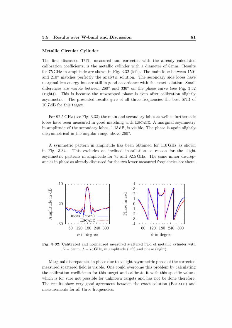
3.5. Results over W-band and Discussion 81
Metallic Circular Cylinder
The first discussed TUT, measured and corrected with the already calculatedcalibration coefficients, is the metallic cylinder with a diameter of 8mm. Resultsfor 75GHz in amplitude are shown in Fig. 3.32 (left). The main lobe between 150◦
and 210◦ matches perfectly the analytic solution. The secondary side lobes havemarginal less energy but are still in good accordance with the exact solution. Smalldifferences are visible between 260◦ and 330◦ on the phase curve (see Fig. 3.32(right)). This is because the unwrapped phase is even after calibration slightlyasymmetric. The presented results give of all three frequencies the best SNR of10.7 dB for this target.
For 92.5GHz (see Fig. 3.33) the main and secondary lobes as well as further sidelobes have been measured in good matching with Escale. A marginal asymmetryin amplitude of the secondary lobes, 1.13 dB, is visible. The phase is again slightlyunsymmetrical in the angular range above 260◦.
A symmetric pattern in amplitude has been obtained for 110GHz as shownin Fig. 3.34. This excludes an inclined installation as reason for the slightasymmetric patterns in amplitude for 75 and 92.5GHz. The same minor discrep-ancies in phase as already discussed for the two lower measured frequencies are there.
-30
-20
-10
60 120 180 240 300
Am
plitud
ein
dB
φ in degree
meas. (corr.)Escale
-4-3-2-101234
60 120 180 240 300
Pha
sein
rad
φ in degree
Fig. 3.32: Calibrated and normalized measured scattered field of metallic cylinder with
D = 8mm, f = 75GHz, in amplitude (left) and phase (right).
Marginal discrepancies in phase due to a slight asymmetric phase of the correctedmeasured scattered field is visible. One could overcome this problem by calculatingthe calibration coefficients for this target and calibrate it with this specific values,which is for sure not possible for unknown targets and has not be done therefore.The results show very good agreement between the exact solution (Escale) andmeasurements for all three frequencies.
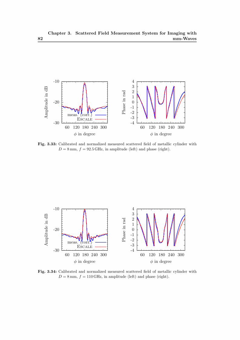
82Chapter 3. Scattered Field Measurement System for Imaging with
mm-Waves
-30
-20
-10
60 120 180 240 300
Am
plitud
ein
dB
φ in degree
meas. (corr.)Escale
-4-3-2-101234
60 120 180 240 300P
hase
inrad
φ in degree
Fig. 3.33: Calibrated and normalized measured scattered field of metallic cylinder with
D = 8mm, f = 92.5GHz, in amplitude (left) and phase (right).
-30
-20
-10
60 120 180 240 300
Am
plitud
ein
dB
φ in degree
meas. (corr.)Escale
-4-3-2-101234
60 120 180 240 300
Pha
sein
rad
φ in degree
Fig. 3.34: Calibrated and normalized measured scattered field of metallic cylinder with
D = 8mm, f = 110GHz, in amplitude (left) and phase (right).

3.5. Results over W-band and Discussion 83
Dielectric Circular Cylinder
The second discussed target is the dielectric cylinder. The material of the cylinderand its geometry have been characterized as explained in detail in Section 3.4.1.The retrieved values have been used for the simulation of the analytic solution forcomparison purposes in the following.
The results for 75GHz are shown in Fig. 3.35. There is a very good matchingbetween the corrected extracted amplitude of the scattered field and the referenceamplitude. The minima are on the same angular positions as foreseen by simulation.The second and third side lobes and the pattern in a zone for φ ∈ [30 · · · 60◦] andfor φ ∈ [270 · · · 330◦] have less energy in measurement as predicted by the analyticsolution. The phase is symmetric after its calibration. Small discrepancies in thephase response over the whole angular area are visible.
Good matching could be obtained in amplitude and in phase for 92.5GHz
as presented in Fig. 3.36. The secondary side lobes in the simulation have lessenergy, 4 dB. The measured phase corresponds well, even in the backscattered re-gion, to the analytic solution. These results give the best SNR (6 dB) for this target.
For 110GHz the number of side lobes in measurement correspond to the one ofthe analytic solution but the lobes have less energy over the whole angular range(see Fig. 3.37). The extracted phase of the measurements is very close, especiallyin the backscattered region, to simulations.
Also the results obtained with a dielectric scatterer correspond to the analyticsolution for all three frequencies. Minor discrepancies occur in amplitude and inphase. This results from the inexact knowledge of the permittivity for certain fre-quencies (75, 92.5 and 110GHz). Further investigations should be done in thecharacterization of the complex relative permittivity for the frequencies of interestin order to provide more reliable simulations.
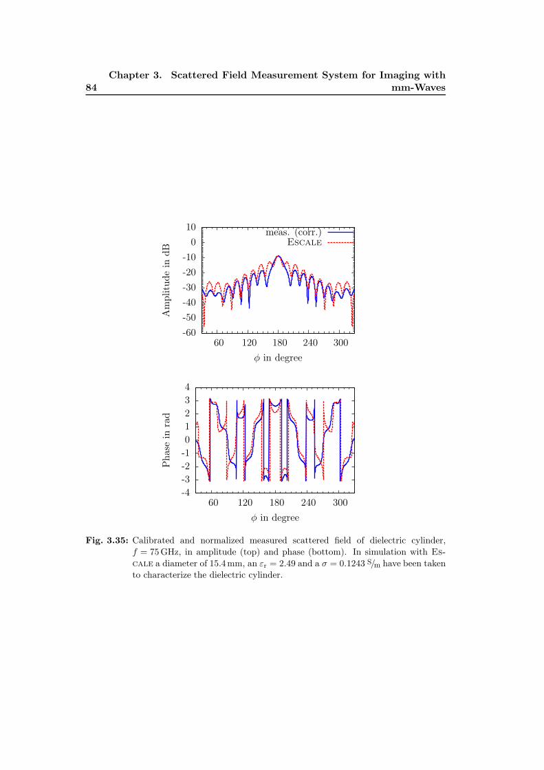
84Chapter 3. Scattered Field Measurement System for Imaging with
mm-Waves
-60
-50
-40
-30
-20
-10
0
10
60 120 180 240 300
Am
plitud
ein
dB
φ in degree
meas. (corr.)Escale
-4-3-2-101234
60 120 180 240 300
Pha
sein
rad
φ in degree
Fig. 3.35: Calibrated and normalized measured scattered field of dielectric cylinder,
f = 75GHz, in amplitude (top) and phase (bottom). In simulation with Es-
cale a diameter of 15.4mm, an εr = 2.49 and a σ = 0.1243 S/m have been taken
to characterize the dielectric cylinder.

3.5. Results over W-band and Discussion 85
-60
-50
-40
-30
-20
-10
0
10
60 120 180 240 300
Am
plitud
ein
dB
φ in degree
meas. (corr.)Escale
-4-3-2-101234
60 120 180 240 300
Pha
sein
rad
φ in degree
Fig. 3.36: Calibrated and normalized measured scattered field of dielectric cylinder,
f = 92.5GHz, in amplitude (top) and phase (bottom). In simulation with Es-
cale a diameter of 15.4mm, an εr = 2.49 and a σ = 0.1243 S/m have been taken
to characterize the dielectric cylinder.

86Chapter 3. Scattered Field Measurement System for Imaging with
mm-Waves
-60
-50
-40
-30
-20
-10
0
10
60 120 180 240 300
Am
plitud
ein
dB
φ in degree
meas. (corr.)Escale
-4-3-2-101234
60 120 180 240 300
Pha
sein
rad
φ in degree
Fig. 3.37: Calibrated and normalized measured scattered field of dielectric cylinder,
f = 110GHz, in amplitude (top) and phase (bottom). In simulation with Es-
cale a diameter of 15.4mm, an εr = 2.49 and a σ = 0.1243 S/m have been taken
to characterize the dielectric cylinder.

3.5. Results over W-band and Discussion 87
3.5.2 Overall Calibration Performance and Measurement Error
The SNR for all three targets and frequencies is summarized in Tab. 3.6 before andafter filtering. As expected, the highest values are obtained for the large cylinder
f in GHzSNR in dB SNR in dB
before filtering after filtering
Metallic cylinder 75 9.02 15.32
D = 20mm92.5 11.54 15.0
110 13.95 15.75
75 9.24 10.70
D = 8mm92.5 9.26 10.34
110 7.85 9.37
Dielectric cylinder 75 3.59 5.56
D = 15mm92.5 4.12 6.0
110 4.79 5.53
Tab. 3.6: The SNR before and after filtering for 1501 points of measurement.
that has been used as reference target for calibration. Before the filtering wasapplied, values varied from 9 to 14 dB. The latter has been obtained for the highestfrequency. After filtering, the SNR is almost constant above 15 dB for all frequencies.For the small cylinder the start SNR is between 7.85 dB for 110GHz and 9.26 dB for92.5GHz. The final values for the SNR are less than for the large cylinder and varyfrom 9.37 dB at 110GHz to 10.7 dB for 75GHz. The dielectric cylinder comes withthe worst SNR. After filtering, where the patterns match well the analytic solution,the best SNR for this target is 6 dB for 92.5GHz.
3.5.3 Mechanical Precision Versus Measurement Error
As mentioned above, working at mm-waves emphases the effects of mechanical er-rors. Therefore, the impact of the swivel arm’s shift has been evaluated versus themeasurement error e (3.10). The latter has been calculated as function of rcircle.For this, simulations were conducted taking into account the swivel arm’s shift.The resulting scattered fields are used as measured fields in the error formula. Themeasurement error versus rcircle for the large cylinder with D = 20mm at 92.5GHz
is plotted in Fig. 3.38.

88Chapter 3. Scattered Field Measurement System for Imaging with
mm-Waves
0
0.1
0.2
0.3
0.4
0.5
0.6
0.7
500 1000
Err
ore
rcircle in µm
rcircle < 165µm
Fig. 3.38: Error e as function of shift rcircle out of the center position, cylinder
D = 20mm, f = 92.5GHz.
Interesting is that a SNR of 15 dB (e = 3.2%), that is our actual value after cali-bration and filtering with the presented slope detection, corresponds to a swivel armpositioning precision of 165µm. This value is relevant since it roughly correspondsto a twentieth of the wavelength. Obtaining this precision is not straightforwardeven with an optical alignment system and is certainly not cost effective, on thecontrary to the post-processing developed in the proposed correction scheme.According to the good performance of the measurement system after calibration,measured data have been used for quantitative imaging as described in the nextchapter.
3.6 Conclusion
In the presented chapter, the scattered field of two different metallic and onedielectric cylinders has been extracted for 75, 92.5 and 110GHz to demonstrate thefeasibility in W-band. For this purpose, a very compact extension to the alreadyexisting equipment in an anechoic chamber has been built: the antennas, whichare small and not very directive, have been mounted very close to the targets.Additionally, the mixers have been located next to the emitting and receivingantennas. Thereby, the mm-wave part is clustered to minimize phase errors due tolong transmitting distances at mm-wave frequencies. For this, we took advantageof the short wavelength value to build a small size system (0.7m× 0.6m) and usedpost-processing to correct misalignment errors as well as to reduce the noise. Anoriginal filtering has been developed that does not require a-priori knowledge ofthe target. This is a key point in the perspective of inversion of unknown objects.It has been successfully applied to measured data and validated in simulationson irregular objects under AWGN. Finally the large metallic cylinder is used as

3.6. Conclusion 89
reference target for deriving the calibration coefficients. Averaged values of thesignal to noise ratio over W-band are 15.4 dB, 10.1 dB and 5.7 dB for the large,the small metallic and the dielectric cylinders respectively. It has been shownthat the proposed system is suitable for providing measurement results whichcan be successfully compared with the exact solution. Furthermore, it has beenpresented that an error in positioning of the target by 1.51mm out of the centerof rotation leads to a high degree of asymmetry in phase. This can be correctedby post-processing and points-out the benefit of having a symmetrical object inorder to calibrate a more complete future system before measuring irregular objects.
Final comparisons obtained from corrected measured values give very good ac-curacy over the whole measured angular range.
Finally, the system sets the first basis for a more complex system capable to han-dle irregular objects. This extension requires an additional rotation of the emittingsection, as this is not possible so far due to the limitation related to the mono-incidence.


Chapter 4
Qualitative and Quantitative
Reconstruction
The objective of this chapter is to validate the measurement system as well as thedone post-processing, presented in the previous chapter, by use of the measurementresults for qualitative and quantitative imaging.
4.1 Qualitative Imaging
In this section the goal is to obtain an image of a field distribution proportional tothe polarization current Jp. Therefore, the complex scattered fields, measured bythe receiver on different positions, have been back-propagated. This has been donefor each frequency separately. This sum, presented in Subsection 2.3.1 (2.57), canbe calculated directly with a matrix multiplication and allows a fast validation ofthe measurements and the applied corrections on one hand. On the other hand,as each field distribution is independently calculated from other cells, large areascan be taken into consideration as well with small pixels to obtain a resolutionwhich corresponds to the physical one, the half of the wavelength. Afterwards, anincoherent sum over these images has been done (2.57) for each frequency and eachemitter.
4.1.1 Localization of Targets
First of all, potential targets have to be detected in general in the whole mea-surement area. Therefore, it has been discretized by cells of λ0,min/0.75 and themeasured complex scattered fields have been back-propagated (Fig. 4.1). Thewavelength λ0,min corresponds to the highest frequency which is 110GHz. Theextracted scattered field from measurements has been directly used. Only anormalization with respect to the maximum of measured amplitudes has beendone in order to overcome differences in the received power levels introduced bythe used measurement equipment over the frequency band of interest. Therefore,no a-priori knowledge of the scatterer is required, which is also advantageous forfuture investigations and drove our choice to this approach for a first validation ofthe measurements. The image indicates the position on a circle of the 1501 pointsof measurement (white circle) as well as the localization of the fixed emitter (redcross). The image is blurred in a zone between the maximum, which corresponds to
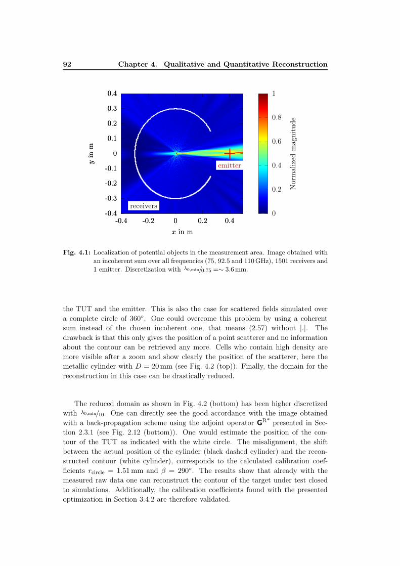
92 Chapter 4. Qualitative and Quantitative Reconstruction
Nor
mal
ized
mag
nitu
de
yin
m
x in m
yin
m
x in m
0
0.2
0.4
0.6
0.8
1
-0.4
-0.3
-0.2
-0.1
0
0.1
0.2
0.3
0.4
-0.4 -0.2 0 0.2 0.4
receivers
emitter
-0.4
-0.3
-0.2
-0.1
0
0.1
0.2
0.3
0.4
-0.4 -0.2 0 0.2 0.4
receivers
emitter
Fig. 4.1: Localization of potential objects in the measurement area. Image obtained with
an incoherent sum over all frequencies (75, 92.5 and 110GHz), 1501 receivers and
1 emitter. Discretization with λ0,min/0.75 =∼ 3.6mm.
the TUT and the emitter. This is also the case for scattered fields simulated overa complete circle of 360◦. One could overcome this problem by using a coherentsum instead of the chosen incoherent one, that means (2.57) without |.|. Thedrawback is that this only gives the position of a point scatterer and no informationabout the contour can be retrieved any more. Cells who contain high density aremore visible after a zoom and show clearly the position of the scatterer, here themetallic cylinder with D = 20mm (see Fig. 4.2 (top)). Finally, the domain for thereconstruction in this case can be drastically reduced.
The reduced domain as shown in Fig. 4.2 (bottom) has been higher discretizedwith λ0,min/10. One can directly see the good accordance with the image obtainedwith a back-propagation scheme using the adjoint operator G
R∗presented in Sec-
tion 2.3.1 (see Fig. 2.12 (bottom)). One would estimate the position of the con-tour of the TUT as indicated with the white circle. The misalignment, the shiftbetween the actual position of the cylinder (black dashed cylinder) and the recon-structed contour (white cylinder), corresponds to the calculated calibration coef-ficients rcircle = 1.51mm and β = 290◦. The results show that already with themeasured raw data one can reconstruct the contour of the target under test closedto simulations. Additionally, the calibration coefficients found with the presentedoptimization in Section 3.4.2 are therefore validated.
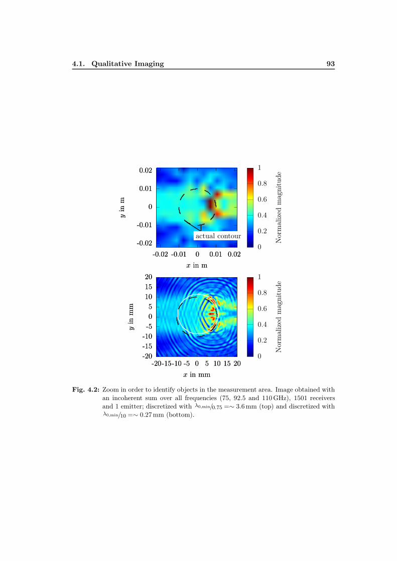
4.1. Qualitative Imaging 93
Nor
mal
ized
mag
nitu
de
yin
m
x in m
yin
m
x in m
0
0.2
0.4
0.6
0.8
1
-0.02
-0.01
0
0.01
0.02
-0.02 -0.01 0 0.01 0.02
actual contour-0.02
-0.01
0
0.01
0.02
-0.02 -0.01 0 0.01 0.02
actual contour
Nor
mal
ized
mag
nitu
de
yin
mm
x in mm
yin
mm
x in mm
0
0.2
0.4
0.6
0.8
1
-20-15-10-505
101520
-20-15-10 -5 0 5 10 15 20-20-15-10-505
101520
-20-15-10 -5 0 5 10 15 20
Fig. 4.2: Zoom in order to identify objects in the measurement area. Image obtained with
an incoherent sum over all frequencies (75, 92.5 and 110GHz), 1501 receivers
and 1 emitter; discretized with λ0,min/0.75 =∼ 3.6mm (top) and discretized withλ0,min/10 =∼ 0.27mm (bottom).

94 Chapter 4. Qualitative and Quantitative Reconstruction
4.1.2 Reconstruction
The extracted scattered fields have been calibrated and filtered. Again, only anormalization with respect to the maximum amplitude has been done as no a-prioriinformation should be preconditioned. That means that for this studies the complexnormalization, explained in Subsection 3.4.3, has not been applied here. The samenormalization has been done with results obtained with the analytic solution forcomparison purposes.
Calibration Target
Results obtained with the presented back-propagation algorithm are shown inFig. 4.3 (left) and compared with simulations (Fig. 4.3 (right)) for the used cal-ibration target. The results based on the calibrated and filtered measurements arein perfect accordance with the simulation. The actual measurement system has pro-
yin
mm
x in mm
yin
mm
x in mm
-20
-10
0
10
20
-20 -10 0 10 20
actual contour-20
-10
0
10
20
-20 -10 0 10 20
actual contour
Nor
mal
ized
mag
nitu
de
x in mmx in mm
0
0.2
0.4
0.6
0.8
1
-20 -10 0 10 20
actual contour
-20 -10 0 10 20
actual contour
Fig. 4.3: Image obtained with an incoherent sum over all frequencies (75, 92.5 and
110GHz), 1501 receivers and 1 emitter for a metallic cylinder of D = 20mm.
Discretization with λ0,min/10 =∼ 0.27mm. Results have been obtained in simu-
lation with Escale (left) and in measurements (right).
vided measurements obtained with one incidence direction (single-incidence case) asthe emitter has been fixed so far.
As the targets of interest have been axially symmetrical, the amplitude and thephase of the scattered fields are symmetrical as well. This is the case after thementioned corrections. That’s why one can expect exactly the same results for anyother incidence direction. Consequently, multi-incidence/multi-view data can beobtained by rotation of the single-incidence/multi-view measurements provided byour setup. Therefore, the same measured and corrected scattered fields have beenshifted 35 times by 10◦ in order to suppose over all 36 emitters. The scattered fieldshave been taken into account for 36 virtual emitters. It has been a trade-off betweenhaving a well described surface of the targets of interest and also an acceptable timefor simulations. In order to improve the results some image-processing can be done:investigations in smoothing and methods to increase the contrast of images basedon radar measurements have been done in [94]. The chosen approach makes use of

4.1. Qualitative Imaging 95
a-priori information on the object to be reconstructed as modeled with homogeneousareas separated by border-like discontinuities. This is the case for all three measuredhomogeneous targets. To enhance the contrast of the final image only pixels whoare at least 3 dB over the averaged image energy have been taken into account. Thisapproach has been already successfully applied to images obtained with a FMCW-radar in the W-band [33] and is here further investigated. Final results are presented
yin
mm
x in mm
yin
mm
x in mm
-20
-10
0
10
20
-20 -10 0 10 20
actual contour-20
-10
0
10
20
-20 -10 0 10 20
actual contour
Nor
mal
ized
mag
nitu
de
x in mmx in mm
0
0.2
0.4
0.6
0.8
1
-20 -10 0 10 20
actual contour
-20 -10 0 10 20
actual contour
Fig. 4.4: Image obtained from measurements with an incoherent sum over all frequencies
(75, 92.5 and 110GHz), 1501 receivers and 36 assumed emitters for a metallic
cylinder of D = 20mm. Discretization with λ0,min/10 =∼ 0.27mm. The image
S (x, y) is presented without processing (left) and with cells having energy at
least 3 dB more than the averaged energy of the image (right).
in Fig. 4.4 and show the main benefit of using millimeter waves. This is the highabsolute resolution provided by the short wavelength. The results show that thereis a perfect accordance between the actual contour of the TUT and the simulation.
Metallic Circular Cylinder
Results after back-propagation for the metallic cylinder of 8mm in diameter, cal-ibrated with the large cylinder, are compared with simulations in Fig. 4.5. Onlyminor differences are visible in the back-scattered region. The image obtained basedon the calibrated measurements is perfectly symmetric which shows the validity ofthe applied post-processing with the presented calibration scheme. Final results areshown in Fig. 4.6. The reconstructed contour corresponds perfectly to the actualone. A zone of strong field distribution of three cells around the actual contour ex-ists which corresponds to a half of the wavelength. The investigated area has beendiscretized with ∆ = λ0,min/10. Three cells are close to the half of the wavelength.That is the theoretical resolution. The maximum of the image corresponds perfectlyto the actual contour.

96 Chapter 4. Qualitative and Quantitative Reconstruction
yin
mm
x in mm
yin
mm
x in mm
-20
-10
0
10
20
-20 -10 0 10 20
actual contour-20
-10
0
10
20
-20 -10 0 10 20
actual contour
Nor
mal
ized
mag
nitu
de
x in mmx in mm
0
0.2
0.4
0.6
0.8
1
-20 -10 0 10 20
actual contour
-20 -10 0 10 20
actual contour
Fig. 4.5: Image obtained with an incoherent sum over all frequencies (75, 92.5 and
110GHz), 1501 receivers and 1 emitter for a metallic cylinder of D = 8mm.
Discretization with λ0,min/10 =∼ 0.27mm. Results have been obtained in simu-
lation with Escale (left) and in measurements (right).
yin
mm
x in mm
yin
mm
x in mm
-20
-10
0
10
20
-20 -10 0 10 20
actual contour-20
-10
0
10
20
-20 -10 0 10 20
actual contour
Nor
mal
ized
mag
nitu
de
x in mmx in mm
0
0.2
0.4
0.6
0.8
1
-20 -10 0 10 20
actual contour
-20 -10 0 10 20
actual contour
Fig. 4.6: Image obtained from measurements with an incoherent sum over all frequencies
(75, 92.5 and 110GHz), 1501 receivers and 36 assumed emitters for a metallic
cylinder of D = 8mm. Discretization with λ0,min/10 =∼ 0.27mm. The image
S (x, y) is presented without processing (left) and with cells having energy at
least 3 dB more than the averaged energy of the image (right).

4.1. Qualitative Imaging 97
Dielectric Circular Cylinder
In Fig. 4.7 results are shown for the target with the worst SNR. Differencesin the field distribution are visible. The zone where the maximum is located,on the opposite side from the emitter, is the same in the image obtained withmeasurements and the one based on simulation. These field distributions aretypical for dielectric objects where strong fields occur due to the reflection at thesurface between air and the dielectric medium [95].
yin
mm
x in mm
yin
mm
x in mm
-20
-10
0
10
20
-20 -10 0 10 20
actual contour-20
-10
0
10
20
-20 -10 0 10 20
actual contour
Nor
mal
ized
mag
nitu
de
x in mmx in mm
0
0.2
0.4
0.6
0.8
1
-20 -10 0 10 20
actual contour
-20 -10 0 10 20
actual contour
Fig. 4.7: Image obtained with an incoherent sum over all frequencies (75, 92.5 and
110GHz), 1501 receivers and 1 emitter for a dielectric cylinder of D = 15mm.
Discretization with λ0,min/10 =∼ 0.27mm. Results have been obtained in simu-
lation with Escale (left) and in measurements (right).
yin
mm
x in mm
yin
mm
x in mm
-20
-10
0
10
20
-20 -10 0 10 20
actual contour-20
-10
0
10
20
-20 -10 0 10 20
actual contour
Nor
mal
ized
mag
nitu
de
x in mmx in mm
0
0.2
0.4
0.6
0.8
1
-20 -10 0 10 20
actual contour
-20 -10 0 10 20
actual contour
Fig. 4.8: Image obtained from measurements with an incoherent sum over all frequencies
(75, 92.5 and 110GHz), 1501 receivers and 36 assumed emitters for a dielectric
cylinder of D = 15mm. Discretization with λ0,min/10 =∼ 0.27mm. The image
S (x, y) is presented without processing (left) and with cells having energy at
least 3 dB more than the averaged energy of the image (right).

98 Chapter 4. Qualitative and Quantitative Reconstruction
Final results are shown in Fig. 4.8. The contour of the dielectric cylinder hasbeen perfectly reconstructed. This has been possible even with an averaged SNRless than 6 dB.
The presented results have shown that the measured results and the applied post-processing are suitable for imaging in the W-band. The contour of two metallic andone dielectric cylinders has been perfectly reconstructed. The contour precision isabout λ0/2 which corresponds to the theoretical limit. Based on the knowledge of thearea for simulation, which is required for reconstruction, a more intensive inverseproblem algorithm has been investigated and results are shown in the next section.
4.2 Quantitative Imaging
In this chapter results obtained with quantitative imaging applied to the alreadymeasured scattered fields are presented.
The in the following presented results were obtained as already mentioned incooperative work with A. Moynot, Ph.D. student at the LEAT, who investigatesthe inverse problem. As the measurement system should be validated we tookadvantage of the already developed inverse problem algorithms successfully appliedto two dimensional objects at LEAT: starting from the direct problem solver thatis an integral representation of the electric field (EFIE), and applying a momentmethod solution, as explained in detail in Subsection 2.2.1, an iterative algorithmis used based on a bi-conjugate gradient method for reconstructing the relative per-mittivity and conductivity (i.e. complex permittivity profile) of the objects undertest. Details on the global procedure of the 2D-inversion have been explained in Sec-tion 2.4. The novelty here is to apply these algorithms in the mm-wave domain now.
The large metallic cylinder has not be taken for inversion as it had been thecalibration target. As so far no regularization scheme has been investigated, thedielectric cylinder is not studied for inversion. Therefore, the small cylinder is usedas object for quantitative reconstruction at the three test frequencies. It requiresthe smallest domain for reconstruction and results in the lowest number of variablesto reconstruct of all three measured targets.
In the past, the quantitative reconstruction has been initialized with or withoutinitial guess, i.e., the starting value is zero contrast. In order to start the iterativeprocedure of a conjugate-gradient method with an initial guess, a back-propagationscheme has been investigated [19, 34, 35, 46]. The iterative algorithm has beendetermined with the specification of the starting value C0 for the contrast. Theconvergence of the algorithm depends also on this initial guess. This has beencalculated with a back-propagation method, using the adjoint operator G
R∗(see
Subsection 2.3.1). This allows to provide an estimate of the induced current Jp inside

4.2. Quantitative Imaging 99
the object. This approach comes with the associated cost of more computation timewith the danger of becoming trapped in a local minimum [42]. That’s why thequantitative inversion has been initialized with a contrast equal to zero. The resultsobtained with the back-propagation have been used to determine the area, whichhas to be discretized for reconstruction. This is an important point because thenumber of cells fixes the time for inversion first and the convergence of the inversiondepends as well mainly on the number of cells.
Before going into the inversion of the results one has to discuss the number ofmeasurement points to take for the inversion. In [96] it is demonstrated that forthe single incidence case with M receivers placed on a circle, the number of pointsM required for the inversion should not exceed:
M = ⌈βD⌉ (4.1)
D being the object diameter and β the propagation constant and ⌈·⌉ gives the firstinteger superior or equal to βD. The value M also represents the number of degreesof freedom for the inversion, therefore, increasing the number of receivers, will betime consuming but not more efficient. Of course, working with a single incidenceis not enough for reconstructing the entire object and in [96] the multi-incidencecriteria is also given. The upper limit for the degrees of freedom is stated withM2/2. Considering that the number of receivers is M we can deduce the number ofemitters as:
L =
⌈M2
2M
⌉, that is L =
⌈M
2
⌉. (4.2)
In our case, having a diameter of 8mm and considering the highest operatingfrequency value of 110GHz one obtains M = 19 and L = 10. Therefore, theinversion should be implemented with 19 receivers and 10 emitters. Considering ourmeasurement step of 0.2◦ the closest possible value for the emitters has been cho-sen that is 12. The number of receivers is 21 (slightly superior than the upper limit).
The 2D-domain for inversion has been discretized for all three frequencies withλ0,min/10 with λ0,min being calculated for the highest frequency of interest which is110GHz. The already presented back-propagation algorithm has been first appliedin order to estimate the size of the domain for inversion.
4.2.1 Estimation of the Domain’s Size
The presented back-propagation has been applied to estimate the domain, whichis further used for the quantitative inversion. Once again, one has to discuss thenumber of receivers M and emitters L which are needed for an accurate estimationof the domain’s size. In our back-propagation algorithm we back-propagate planewaves. When the object is within a pixel this latter provides a higher signal than forpixels without object. The signal level also depends on the direction of the incidence:
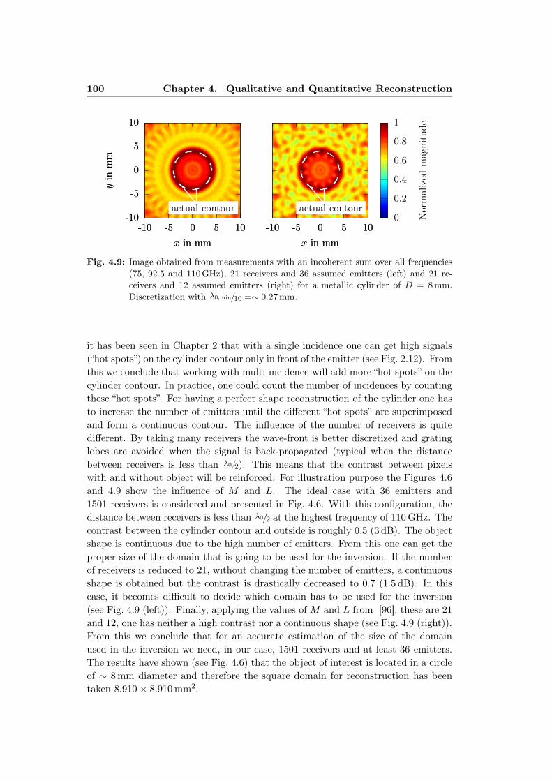
100 Chapter 4. Qualitative and Quantitative Reconstruction
yin
mm
x in mm
yin
mm
x in mm
-10
-5
0
5
10
-10 -5 0 5 10
actual contour-10
-5
0
5
10
-10 -5 0 5 10
actual contour
Nor
mal
ized
mag
nitu
de
x in mmx in mm
0
0.2
0.4
0.6
0.8
1
-10 -5 0 5 10
actual contour
-10 -5 0 5 10
actual contour
Fig. 4.9: Image obtained from measurements with an incoherent sum over all frequencies
(75, 92.5 and 110GHz), 21 receivers and 36 assumed emitters (left) and 21 re-
ceivers and 12 assumed emitters (right) for a metallic cylinder of D = 8mm.
Discretization with λ0,min/10 =∼ 0.27mm.
it has been seen in Chapter 2 that with a single incidence one can get high signals(“hot spots”) on the cylinder contour only in front of the emitter (see Fig. 2.12). Fromthis we conclude that working with multi-incidence will add more “hot spots” on thecylinder contour. In practice, one could count the number of incidences by countingthese “hot spots”. For having a perfect shape reconstruction of the cylinder one hasto increase the number of emitters until the different “hot spots” are superimposedand form a continuous contour. The influence of the number of receivers is quitedifferent. By taking many receivers the wave-front is better discretized and gratinglobes are avoided when the signal is back-propagated (typical when the distancebetween receivers is less than λ0/2). This means that the contrast between pixelswith and without object will be reinforced. For illustration purpose the Figures 4.6and 4.9 show the influence of M and L. The ideal case with 36 emitters and1501 receivers is considered and presented in Fig. 4.6. With this configuration, thedistance between receivers is less than λ0/2 at the highest frequency of 110GHz. Thecontrast between the cylinder contour and outside is roughly 0.5 (3 dB). The objectshape is continuous due to the high number of emitters. From this one can get theproper size of the domain that is going to be used for the inversion. If the numberof receivers is reduced to 21, without changing the number of emitters, a continuousshape is obtained but the contrast is drastically decreased to 0.7 (1.5 dB). In thiscase, it becomes difficult to decide which domain has to be used for the inversion(see Fig. 4.9 (left)). Finally, applying the values of M and L from [96], these are 21
and 12, one has neither a high contrast nor a continuous shape (see Fig. 4.9 (right)).From this we conclude that for an accurate estimation of the size of the domainused in the inversion we need, in our case, 1501 receivers and at least 36 emitters.The results have shown (see Fig. 4.6) that the object of interest is located in a circleof ∼ 8mm diameter and therefore the square domain for reconstruction has beentaken 8.910 × 8.910mm2.

4.2. Quantitative Imaging 101
4.2.2 Expected Complex Permittivity Values
The next step is to apply the inverse problem algorithm. Before going into recon-struction results, one has to discuss about expected complex permittivity values.Metallic targets have been investigated in simulations with a relative permittivityof 1 and conductivity values usually up to several MS/m. Nevertheless, lower fre-quency reconstructions [19] have shown that conductivity values of 7 to 8 S/m wereretrieved for metallic objects. The reasons that limit the actual sigma values is thelack of significant difference between scattered field results when sigma reaches acertain value. In the Subsection 2.4.2 expected sigma values as function of the SNRhave been theoretically investigated. The shown results cannot be taken directly asreference for expected values obtained by the inversion. As shown in Fig. 2.15 onegets for an SNR of 10 dB, which can be obtained in measurements with the smallmetallic cylinder, a sigma between 25 S/m and 50 S/m. This shows the introducedSNR by approximation a PEC with a cylinder having a finite conductivity by tak-ing the exact solution. One has also to take into account the influence of the usedalgorithm to calculate the direct problem, who introduces numerical noise due tothe discretization of the domain. In order to estimate it, the SNR has been againcomputed versus sigma values. The reference signal, the exact solution, assumes aninfinite conductivity whereas sigma values are varying for E(s)
sim.,norm. calculated withFlexiMoM. SNR versus sigma has been computed at the central frequency of theW-band. The results presented in Fig. 4.10 show logically that the SNR increaseswith sigma but also that it saturates for values of sigma far below the physical orderof magnitude of several MS/m.
456789
1011
10 20 30 40 50 60 70 80 90 100
SNR
indB
σ in Sm
Fig. 4.10: SNR calculated as function of σ for 751 receivers, cylinder D = 8mm,
f = 92.5GHz. The expected value of sigma after reconstruction is indicated
based on the SNR of the calibrated and normalized measurements.
4.2.3 Inversion Results
In a first step results are presented for 751 receivers. The extracted scattered fieldshave been used for reconstruction after its calibration, filtering and normalization.

102 Chapter 4. Qualitative and Quantitative Reconstruction
This has been done for 751 points of measurement that means every second pointis taken from the 1501 available points in order to accelerate the process to ob-tain rapidly first results. Simulations with 1501 has been investigated but onlymarginal differences have been visible. A-priori information concerning the rangeof the searched values of the permittivity and conductivity profiles can be easilyincorporated in the reconstruction algorithm. Therefore, a study on the influence ofa-priori information (minimum and maximum values) of the complex permittivityis quite of interest. For the results presented hereafter, the minimum and maxi-mum values for the permittivity and conductivity are, respectively, εr,min = 1.0,εr,max = 1.2; σmin = 0 S/m, σmax = 100 S/m. Results after 100 iterations are shownin Fig. 4.11.
yin
mm
x in mm
11.021.041.061.081.11.121.141.161.181.2
-4-3-2-101234
-4 -3 -2 -1 0 1 2 3 4
εr
x in mm
02468101214
-4 -3 -2 -1 0 1 2 3 4
σ in S/m
Fig. 4.11: The relative permittivity (left) and the conductivity (right) reconstructed
with 100 iterations (751 receivers, 1 emitter, 92.5GHz, discretization with
0.27mm ≈ λ0,min/10). Scattered fields of the cylinder, D = 8mm, have been
measured in a distance of 300mm.
As expected, for the one emitter configuration almost one half of the contourcould be retrieved as it has been also the case with the back-propagation scheme.The maximum value for the conductivity is 14.79 S/m. Minor discrepancies in sym-metry haven’t been visible anymore in results obtained with the back-propagation.Here the asymmetry results in small deviations of the calculated values of εr and σ.
The symmetry of the results has been again taken into account as already donefor the back-propagation scheme and has been explained in Subsection 4.1.2. There-fore, the number of illuminations symmetrizing the set of measurements has beenincreased in order to simulate different number of angles (8, 12, 15 and 18 angles ofincidence). Results are presented in [123].
Results of reconstruction after 100 iterations for 75GHz are shown in Fig. 4.12.

4.2. Quantitative Imaging 103
yin
mm
x in mm
11.021.041.061.081.11.121.141.161.181.2
-4-3-2-101234
-4 -3 -2 -1 0 1 2 3 4
εr
x in mm
02468101214
-4 -3 -2 -1 0 1 2 3 4
σ in S/m
Fig. 4.12: The relative permittivity (left) and the conductivity (right) reconstructed
with 100 iterations (751 receivers, 15 emitters, 75GHz, discretization with
0.27mm ≈ λ0,min/10). Scattered fields of the cylinder, D = 8mm, have been
measured in a distance of 300mm.
At this frequency the best SNR for this target, 11.7 dB, has been provided.The results are in perfect accordance with the actual contour of the cylinder. Themaximum sigma value on the reconstructed contour is 15.54 S/m.
For the center frequency, where a SNR of 10.34 dB has been obtained, theresults are presented in Fig. 4.13.
yin
mm
x in mm
11.021.041.061.081.11.121.141.161.181.2
-4-3-2-101234
-4 -3 -2 -1 0 1 2 3 4
εr
x in mm
0246810121416
-4 -3 -2 -1 0 1 2 3 4
σ in S/m
Fig. 4.13: The relative permittivity (left) and the conductivity (right) reconstructed
with 100 iterations (751 receivers, 15 emitters, 92.5GHz, discretization with
0.27mm ≈ λ0,min/10). Scattered fields of the cylinder, D = 8mm, have been
measured in a distance of 300mm.
Again, the contour of the cylinder could be perfectly reconstructed with amaximum value for sigma of 16.83 S/m.
For the highest frequency the results for the complex permittivity are shownin Fig. 4.14. This frequency corresponds to the worst case for the quality of theinput data (i.e. measured scattered fields) with a SNR of 9.37 dB as well as for

104 Chapter 4. Qualitative and Quantitative Reconstruction
the inversion algorithm because it is where the domain has the lowest discretization.y
inm
m
x in mm
11.021.041.061.081.11.121.141.161.181.2
-4-3-2-101234
-4 -3 -2 -1 0 1 2 3 4
εr
x in mm
024681012141618
-4 -3 -2 -1 0 1 2 3 4
σ in S/m
Fig. 4.14: The relative permittivity (left) and the conductivity (right) reconstructed
with 100 iterations (751 receivers, 15 emitters, 110GHz, discretization with
0.27mm ≈ λ0,min/10). Scattered fields of the cylinder, D = 8mm, have been
measured in a distance of 300mm.
The Fig. 4.15 demonstrates that the presented results for 110GHz have beenobtained with the worst convergence of the cost function J(C).
0.1
0.2
0.3
0.4
0 10 20 30 40 50 60 70 80 90100
Nor
mal
ized
cost
valu
e
Iterations
f = 75.0GHzf = 92.5GHzf = 110.0 GHz
Fig. 4.15: Normalized cost values for each iteration obtained for 75, 92.5 and 110GHz
separately.
The contour of the cylinder has been retrieved with a sigma value of 19.62 S/m.This is almost three times higher than at lower frequencies (10GHz, [19]). Forthe so far presented results one can conclude that with increasing frequency theobtained sigma value also increases.
In order to improve the former results (that is to retrieve higher values for sigma),the number of receivers and emitters is now chosen according to [96]. Because of thediscretization of 0.2◦ of the measured field we cannot exactly match the 19 receiversand 10 emitters and have to chose 21 receivers and 12 emitters. Results are shownin Fig. 4.16, Fig. 4.17 and Fig. 4.18 for 75GHz, 92.5GHz and 110GHz respectively.

4.2. Quantitative Imaging 105
yin
mm
x in mm
11.021.041.061.081.11.121.141.161.181.2
-4-3-2-101234
-4 -3 -2 -1 0 1 2 3 4
εr
x in mm
010203040506070
-4 -3 -2 -1 0 1 2 3 4
σ in S/m
Fig. 4.16: The relative permittivity (left) and the conductivity (right) reconstructed
with 1000 iterations (21 receivers, 12 emitters, 75GHz, discretization with
0.27mm ≈ λ0,min/10). Scattered fields of the cylinder, D = 8mm, have been
measured in a distance of 300mm.
yin
mm
x in mm
11.021.041.061.081.11.121.141.161.181.2
-4-3-2-101234
-4 -3 -2 -1 0 1 2 3 4
εr
x in mm
010203040506070
-4 -3 -2 -1 0 1 2 3 4
σ in S/m
Fig. 4.17: The relative permittivity (left) and the conductivity (right) reconstructed
with 1000 iterations (21 receivers, 12 emitters, 92.5GHz, discretization with
0.27mm ≈ λ0,min/10). Scattered fields of the cylinder, D = 8mm, have been
measured in a distance of 300mm.
yin
mm
x in mm
11.021.041.061.081.11.121.141.161.181.2
-4-3-2-101234
-4 -3 -2 -1 0 1 2 3 4
εr
x in mm
010203040506070
-4 -3 -2 -1 0 1 2 3 4
σ in S/m
Fig. 4.18: The relative permittivity (left) and the conductivity (right) reconstructed
with 1000 iterations (21 receivers, 12 emitters, 110GHz, discretization with
0.27mm ≈ λ0,min/10). Scattered fields of the cylinder, D = 8mm, have been
measured in a distance of 300mm.

106 Chapter 4. Qualitative and Quantitative Reconstruction
Interesting is, that the values of sigma (the maxima are 77.37 S/m, 81.12 S/mand 81.08 S/m for 75GHz, 92.5GHz and 110GHz) have now a scaling factor of 8
compared to the low frequency results at 10GHz [19] that matches the frequencyscaling factor. Together with the increase of sigma a better contrast between thecylinder contour and the rest of the domain is obtained.
4.3 Conclusion
In a first step, the contour of all three targets has been precisely reconstructed witha fast back-propagation scheme. In a second step, this results have been used toestimate the area for simulations with an inverse problem algorithm. The increase ofthe reconstructed values of sigma with higher frequencies points out the advantageof the short wavelength. The conjugate gradient algorithm presented here, andapplied to measured scattered data has shown its effectiveness in the reconstructionof metallic objects. This method can be applied to any kind of lossy dielectricobjects. Further investigations are going to be the reconstruction based on extractedscattered fields of the measured acrylic cylinder in future.

Chapter 5
FMCW-Radar Measurements
5.1 Introduction of Application
The so far presented investigations have been done in a laboratory environment:the targets of interest have been isolated. Therefore, it has been possible to measurethe scattered field with a set of receivers surrounding the TUT. Additionally, thestudied objects have been embedded in an homogeneous background. The targetshave been successfully localized and qualitatively and quantitatively retrieved. Forpractical applications the number of receivers is drastically limited. Additionally,the objects of interest can be found in an inhomogeneous environment. Millimeter-wave systems are already used for the detection and localization of small objectsdue to the high resolution provided by the small wave-length. These systemsare pushed to identification nowadays that means the extension to imaging. Inthe following, the motivation of the chosen application, the detection of FOD,is introduced. Furthermore, the limitations of detection capabilities should beinvestigated with a mm-wave system assembled with two transmitters to set a firstbasis to estimate possibilities for quantitative imaging in future in the W-band.
The detection of FOD on airports becomes more and more important. It hasbeen estimated that FOD damage costs the aerospace industry over $4 billion(US) per year, mostly in the costs associated with engine damage and loss of useof the aircraft. At its worst, FOD can lead to loss of life as seen in the Concordeaccident of July 2000. Air France Flight 4590 crashed after departing from Charlesde Gaulle International Airport near Paris, France. The aircraft had run over apiece of titanium debris on the runway.Since over 5 years, several companies have developed, proposed and tested auto-mated FOD detection systems. Different approaches have been investigated: theTarsier by QinetiQ [97] is based on mm-wave radar modules operating around94.5GHz and has been recently completed by a camera for identification purposes.Two large radar modules are necessary for covering one runway. On the other hand,optical-based systems have also been proposed: they are based on CCD camera,LIDAR or LADAR equipments [98,99]. The latter are the most performing regard-ing identification capabilities but performances are greatly decreased under badweather conditions. Another approach also uses millimeter-wave radar but withinthe 77GHz band [100, 101]. Although it is less favorable than the 94GHz one forpropagation, it benefits from the low-cost MMICs developed for the automotivecruise control application. In addition to that, the possibility to work with a

108 Chapter 5. FMCW-Radar Measurements
bandwidth of 5GHz improves the range resolution [116,118]. Trex Enterprise’s
FODFinder, that uses infrared cameras and mm-wave radar mounted on the roofof a vehicle, provides FOD detection also on taxiways, apron areas etc. due to itsmobility [102]. The LaotSe project investigates up to 220GHz. The systemcomprises an infrared camera, optical 2D and 3D cameras, and networked radarsensors [103]. Some of the above mentioned approaches [97, 98, 101, 102] havebeen already evaluated by the Federal Aviation Administration (FAA) in order todevelop performance standards for FOD detection systems [104].
The chosen system configuration for our study is shown in Fig. 5.1 [8] [121].The FOD detection system consists of several small low power and low cost sensors,developed within the work presented in [69, 105], placed near the runway, each ofthem covering a given part of it.
Up to now, the two-dimensional back scattering map of the runway surfacehas been obtained by mechanically scanning the sensor. The following approach,presented in Section 2.3.2, is different: it has been shown that imaging is possibleby performing separate measurements from two different positions using wide-beam-width antennas [2, 68, 106] for 24GHz at least in the close range. This approachis investigated in the following in the W-band firstly with a vector measurementequipment and secondly with a mm-wave radar system.
antenna
runway
antenna
FOD
runway
Fig. 5.1: Runway surveillance system consisting of mm-wave sensors located at both sides
of the runway.
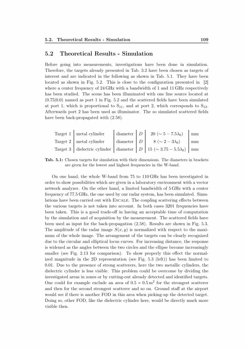
5.2. Theoretical Results - Simulation 109
5.2 Theoretical Results - Simulation
Before going into measurements, investigations have been done in simulation.Therefore, the targets already presented in Tab. 3.2 have been chosen as targets ofinterest and are indicated in the following as shown in Tab. 5.1. They have beenlocated as shown in Fig. 5.2. This is close to the configuration presented in [2]where a center frequency of 24GHz with a bandwidth of 1 and 11GHz respectivelyhas been studied. The scene has been illuminated with one line source located at(0.75|0.0) named as port 1 in Fig. 5.2 and the scattered fields have been simulatedat port 1, which is proportional to S11, and at port 2, which corresponds to S12.Afterwards port 2 has been used as illuminator. The so simulated scattered fieldshave been back-propagated with (2.58).
Target 1 metal cylinder diameter D 20 (∼ 5− 7.5λ0) mm
Target 2 metal cylinder diameter D 8 (∼ 2− 3λ0) mm
Target 3 dielectric cylinder diameter D 15 (∼ 3.75− 5.5λ0) mm
Tab. 5.1: Chosen targets for simulation with their dimensions. The diameters in brackets
are given for the lowest and highest frequencies in the W-band.
On one hand, the whole W-band from 75 to 110GHz has been investigated inorder to show possibilities which are given in a laboratory environment with a vectornetwork analyzer. On the other hand, a limited bandwidth of 5GHz with a centerfrequency of 77.5GHz, the one used by our radar system, has been simulated. Simu-lations have been carried out with Escale. The coupling scattering effects betweenthe various targets is not taken into account. In both cases 3201 frequencies havebeen taken. This is a good trade-off in having an acceptable time of computationby the simulation and of acquisition by the measurement. The scattered fields havebeen used as input for the back-propagation (2.58). Results are shown in Fig. 5.3.The amplitude of the radar image S(x, y) is normalized with respect to the maxi-mum of the whole image. The arrangement of the targets can be clearly recognizeddue to the circular and elliptical locus curves. For increasing distance, the responseis widened as the angles between the two circles and the ellipse become increasinglysmaller (see Fig. 2.13 for comparison). To show properly this effect the normal-ized magnitude in the 2D representation (see Fig. 5.3 (left)) has been limited to0.01. Due to the presence of strong scatterers, here the two metallic cylinders, thedielectric cylinder is less visible. This problem could be overcome by dividing theinvestigated areas in zones or by cutting-out already detected and identified targets.One could for example exclude an area of 0.5 × 0.5m2 for the strongest scattererand then for the second strongest scatterer and so on. Ground staff at the airportwould see if there is another FOD in this area when picking-up the detected target.Doing so, other FOD, like the dielectric cylinder here, would be directly much morevisible then.

110 Chapter 5. FMCW-Radar Measurements
port 1(0.75|0.00)(187.5λ0|0)
port 2(−0.75|0.00)(−187.5λ0|0)
target 1(−0.70|3.70)(−175λ0|925λ0)
target 2(0.80|2.60)(200λ0|650λ0)
target 3(−0.50|1.50)(−125λ0|375λ0)
x
y
2m (500λ0)
3m
(750λ0)
(0.0|0.0)
Fig. 5.2: Geometrical arrangement of two metal and one dielectric cylinders. Coordinates
are given in meters and in terms of λ0 for 75GHz. The area inside the green
rectangle 2× 3m2 is used for further reconstructions.
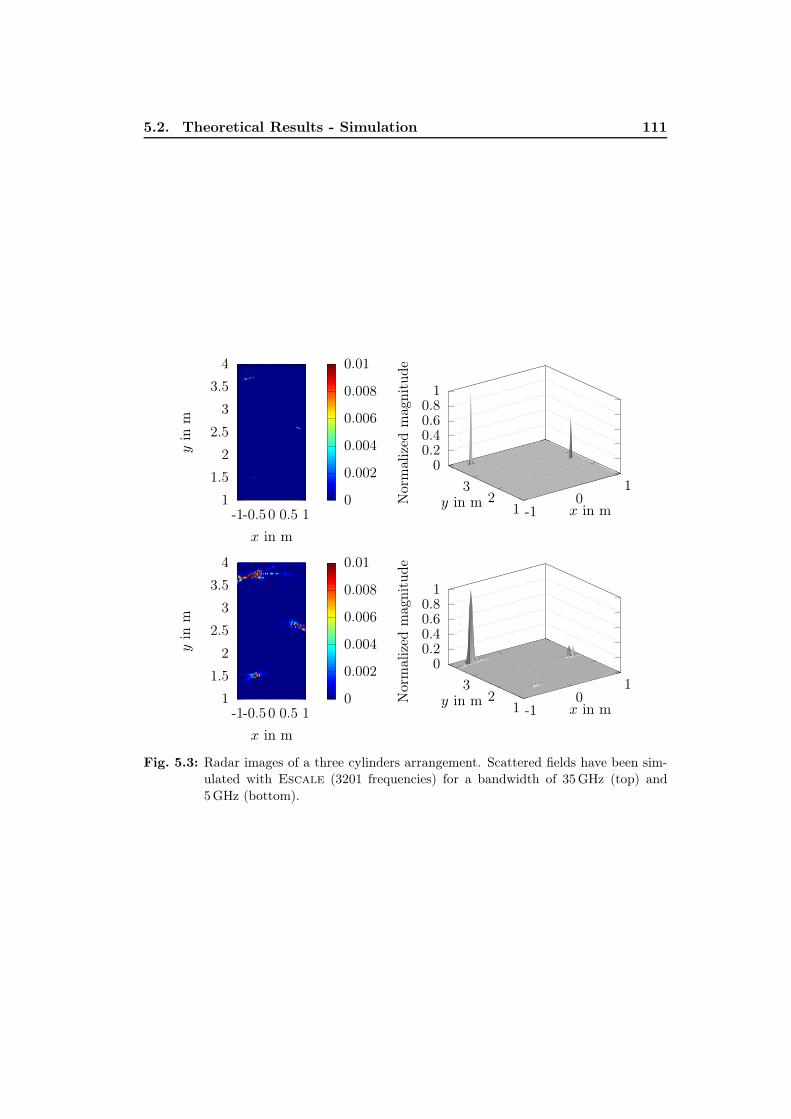
5.2. Theoretical Results - Simulation 111
Nor
mal
ized
mag
nitu
de
yin
m
x in m
0
0.002
0.004
0.006
0.008
0.01
1
1.5
2
2.5
3
3.5
4
-1-0.5 0 0.5 1 -10
1
12
3
00.20.40.60.8
1
x in my in m
Nor
mal
ized
mag
nitu
de
yin
m
x in m
0
0.002
0.004
0.006
0.008
0.01
1
1.5
2
2.5
3
3.5
4
-1-0.5 0 0.5 1 -10
1
12
3
00.20.40.60.8
1
x in my in m
Fig. 5.3: Radar images of a three cylinders arrangement. Scattered fields have been sim-
ulated with Escale (3201 frequencies) for a bandwidth of 35GHz (top) and
5GHz (bottom).
112 Chapter 5. FMCW-Radar Measurements
5.3 Ideal Setup with Network Analyzer
In a first step, the simulated configuration with the both metallic and the dielectriccylinders has been investigated in measurements with a network analyzer. In asecond step, real FOD are measured and results presented hereinafter.
5.3.1 Scene with Vertical Cylinders
Measurements have been done in a class room. In order to reduce reflections fromtables and walls to a minimum they have been covered by absorber material asshown in Fig. 5.4 (bottom). The setup with the network analyzer in combinationwith mm-wave heads is presented in Fig. 5.4 (top). The measurements have beendone with Agilent’s PNA-X microwave network analyzer in combination withmm-wave modules [83, 84]. As shown in Fig. 5.4 (top) a stand alone vectornetwork analyzer has been used as the so far presented equipment of the anechoicchamber, presented in Chapter 3, remains there as it is used permanently forantenna measurements.
Open ended waveguides have been used as antennas in order to have a wideillumination of the area of interest.
First, a measurement without the targets of interest has been done to measure
the incident field(A
(i)z ,Φ(i)
)in amplitude and in phase. Then, the cylinders have
been installed and the total field has been measured(A
(t)z ,Φ(t)
). Again with a
vectorial subtraction the scattered fields of the targets of interest(A
(s)z ,Φ(s)
)have
been extracted. For the free space measurements the supports have already beentaken into account. Results have shown, at least for the dielectric cylinder, thatscattered fields from the target support have been dominant compared to the onesof the target of interest itself. The obtained radar images are shown in Fig. 5.5and Fig. 5.6. The results are in excellent accordance with the simulations for abandwidth of 35 as well as of 5GHz.

5.3. Ideal Setup with Network Analyzer 113
Fig. 5.4: Photograph of a three cylinders arrangement inside. Setup of the analyzer with
two open ended waveguides as antennas (top). Scene of the three cylinders (bot-
tom).

114 Chapter 5. FMCW-Radar Measurements
Nor
mal
ized
mag
nitu
de
yin
m
x in m
0
0.002
0.004
0.006
0.008
0.01
1
1.5
2
2.5
3
3.5
4
-1 -0.5 0 0.5 1
-10
1
12
3
00.20.40.60.8
1
Normalized magnitude
x in my in m
Fig. 5.5: Radar images of a three cylinders arrangement. Measurements have been done
with the network analyzer (3201 frequencies) for a bandwidth of 35GHz.

5.3. Ideal Setup with Network Analyzer 115
Nor
mal
ized
mag
nitu
de
yin
m
x in m
0
0.002
0.004
0.006
0.008
0.01
1
1.5
2
2.5
3
3.5
4
-1 -0.5 0 0.5 1
-10
1
12
3
00.20.40.60.8
1
Normalized magnitude
x in my in m
Fig. 5.6: Radar images of a three cylinders arrangement. Measurements have been done
with the network analyzer (3201 frequencies) for a bandwidth of 5GHz.
116 Chapter 5. FMCW-Radar Measurements
5.3.2 Detection of Foreign Object Debris
After this preliminary investigations in simulation and measurement with regulartargets, “real” FOD have been considered. These objects have been found on runwaysat Charles de Gaulle airport in Paris, France. The TUT are summarized in Tab. 5.2.A photo of the scene and of the FOD in detail is shown in Fig. 5.7. Radar images are
Description Position (x|y) in meter
FOD 1 piece of plane (−0.70|3.40)FOD 2 piece of plane brake (−0.80|2.30)FOD 3 plane tank cap (−0.50|1.20)
Tab. 5.2: Description and position of investigated FOD. Positions are referenced to the
center point (0.0|0.0) between the two antennas (see Fig. 5.2).
shown in Fig. 5.8 and in Fig. 5.9. The arrangement of all three FOD can be clearlyrecognized. Even the small pieces of a plane brake have been perfectly retrievedwith a bandwidth of 5GHz. All these results have been evaluated without specialwindowing. As explained in Section 2.3.2 the resolution raises with increasingbandwidth. Therefore, the maxima become larger for potential targets in the imagefor a smaller bandwidth. That’s why the targets can be more easily recognized bythe eye for the measurements done with ∆f = 5GHz.

5.3. Ideal Setup with Network Analyzer 117
FOD 1 FOD 2 FOD 3
Fig. 5.7: Photograph of an arrangement inside with three FOD. Scene with the position of
the FOD (top). The three FOD in detail (bottom). The red markers correspond
to the point used as reference where the targets are located in the coordinate
system.

118 Chapter 5. FMCW-Radar Measurements
Nor
mal
ized
mag
nitu
de
yin
m
x in m
0
0.05
0.1
0.15
0.2
0.25
0.3
0.35
0.4
1
1.5
2
2.5
3
3.5
4
-1 -0.5 0 0.5 1
-10
1
12
3
00.20.40.60.8
1
Normalized magnitude
x in my in m
Fig. 5.8: Radar images of a three FOD arrangement. Measurements have been done with
the network analyzer for a bandwidth of 35GHz.

5.3. Ideal Setup with Network Analyzer 119
Nor
mal
ized
mag
nitu
de
yin
m
x in m
0
0.05
0.1
0.15
0.2
0.25
0.3
0.35
0.4
1
1.5
2
2.5
3
3.5
4
-1 -0.5 0 0.5 1
-10
1
12
3
00.20.40.60.8
1
Normalized magnitude
x in my in m
Fig. 5.9: Radar images of a three FOD arrangement. Measurements have been done with
the network analyzer for a bandwidth of 5GHz.
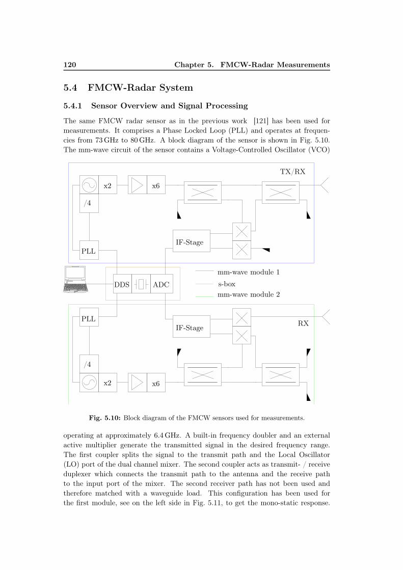
120 Chapter 5. FMCW-Radar Measurements
5.4 FMCW-Radar System
5.4.1 Sensor Overview and Signal Processing
The same FMCW radar sensor as in the previous work [121] has been used formeasurements. It comprises a Phase Locked Loop (PLL) and operates at frequen-cies from 73GHz to 80GHz. A block diagram of the sensor is shown in Fig. 5.10.The mm-wave circuit of the sensor contains a Voltage-Controlled Oscillator (VCO)
x2
x2
x6
x6
/4
/4
PLL
PLL
DDS ADC
IF-Stage
IF-Stage
TX/RX
RX
mm-wave module 1
s-box
mm-wave module 2
Fig. 5.10: Block diagram of the FMCW sensors used for measurements.
operating at approximately 6.4GHz. A built-in frequency doubler and an externalactive multiplier generate the transmitted signal in the desired frequency range.The first coupler splits the signal to the transmit path and the Local Oscillator(LO) port of the dual channel mixer. The second coupler acts as transmit- / receiveduplexer which connects the transmit path to the antenna and the receive pathto the input port of the mixer. The second receiver path has not been used andtherefore matched with a waveguide load. This configuration has been used forthe first module, see on the left side in Fig. 5.11, to get the mono-static response.

5.4. FMCW-Radar System 121
Fig. 5.11: Photograph of the setup with the radar system with a standard gain horn as
antenna.
To obtain the bi-static response with the second module, see on the right side inFig. 5.11, the receiver path has been connected with the antenna and the transmitpath has been matched with a wave-guide load.
The core of the FMCW sensor is a synthesizer based on a PLL and Direct Dig-ital Synthesis (DDS). The linear frequency modulated base band signal is digitallygenerated at frequencies lower than 25MHz. This signal serves as reference signalof the PLL which controls the VCO. An important feature of the sensor is that theclock for the DDS and the Analogue Digital Conversion unit (ADC) are both derivedfrom the same crystal oscillator. Therefore, not only the frequency synthesis butalso the data acquisition are phase-locked to a very stable reference. This offers thepossibility to coherently sum up subsequent radar measurements and in consequenceimprove the SNR. The setup in Fig. 5.11 shows the two mm-wave modules. Bothhave been driven by two synchronized DDS in one s-box (see Fig. 5.10). The seconds-box is only used as power supply for the second mm-wave module. In order toprovide a configuration similar to the one presented in Section 5.3 with the networkanalyzer the following steps have been done: the first mm-wave module, used inTX/RX configuration, has been mounted on the position, where the port 1 was.With it the mono-static radar response for this position has been retrieved. Thesecond mm-wave module, located at the position where the port 2 was, has beenused to obtain the bi-static radar response. Afterwards, the position of the moduleshas been manually changed to get the mono-static response from port 2 and thebi-static one from port 1.
Before presenting the measurement process a short description of retrieved valueswith the FMCW radar system should be given hereinafter. The received signal (RX)is an attenuated copy of the transmitted signal (TX), delayed by one round trip delayτ = 2R/c0 between sensor and the target as shown in Fig. 5.12. The slope of thelinear frequency modulation can be defined as:
S =∆f
T. (5.1)
Knowing this, the intermediate frequency can be written as:
fIF = S∆T. (5.2)

122 Chapter 5. FMCW-Radar Measurements
t
t
f(t)
f(t)
0
0
τ
τ
T
T
f0
f0
f0 +∆f
TX
RX
fIF
Fig. 5.12: Instantaneous frequencies of transmitted (TX), received (RX) and intermediate
frequency (IF) signal.
For FMCW radars the IF-time domain samples directly provide the RF-frequency domain representation of the channel response. In the following, theIF signal in the frequency domain is directly taken. In the used FMCW radar noI/Q receiver is used. So only the real part of the complex frequency response ismeasured. As the pulse response of the radar channel is a causal and real valuedsignal, the imaginary part can be calculated using the Hilbert transform [70, 105].Following, the already presented back-propagation algorithm is applied.
5.4.2 Measurement Results
Measurements have been done from 75GHz to 80GHz. There the output powerof the sensors varies from 5 dBm to 9 dBm. This is less than the output power ofthe vector network analyzer equipment. For this reason, standard gain horns havehad to be used as antennas. Their radiation patterns reduce drastically the areaof interest for measurements as shown in Fig. 5.13. In order to detect the TUTwith both sensors the targets have been located in a distance larger than 4.3m.Measurements have been done for 3201 frequencies as with the network analyzer.This results in a ramp duration of T = 512 µs with the fixed sampling frequency ofthe ADC of 6.25MHz. To improve the signal to noise ratio 16 measurements havebeen integrated. The overall coherency of the system makes it possible to calibratethe measurements by acquiring an empty scene measurement and subtracting thesedata from the actual measurements as done with the network analyzer. Processingof the IF signals has been done in a manner which is typical for FMCW sensors:the sampled data have been weighted using a Chebyschev window with a side lobesuppression of 60 dB [107], resulting in a much better visibility of the targets in

5.4. FMCW-Radar System 123
the radar image.
The scene of interest is shown in Fig. 5.14. The investigated targets are summa-rized in Tab. 5.3.
0
1
2
3
4
5
6
-1 0 1
yin
met
er
x in meter
standard gain horn: −3 dBstandard gain horn: −6 dB
open ended waveguide
Fig. 5.13: Zone covered by the antennas. The angles for the 3 dB- and 6 dB-beam-width
have been plotted as function of x and y.
Description Diameter D Position (x|y) in meter
Cylinder 1 metallic cylinder 70mm (−0.8|11.6)Cylinder 2 metallic cylinder 20mm (0.5|9.7)Cylinder 3 dielectric cylinder 70mm (0.0|5.8)
Tab. 5.3: Description and the approximate position of the investigated cylinders. The
positions are referenced to the center point (0.0|0.0) between the two antennas.
Unfortunately, no meaningful bi-static response could be measured with thepresented setup. This might be due to different propagation delays in the cablesused to connect the sensor modules with the s-box. The cables between the s-boxand the modules did not have the same length. Additionally, the two DDS mightnot work totally synchronize. For this reason, only images obtained with the mono-static radar response are presented in the following. All three cylinders have beendetected as shown in Fig. 5.15. Furthermore, the advantage of having a short rampduration should be shown. It has been demonstrated in [109], that fast modulationramps have the benefit to increase the delta between two IF signals and comes witha lower sensitivity to phase noise. For comparison, 30000 frequencies have beenused for the same ∆f = 5GHz. This leads to a ramp duration of T = 4.8ms. Theobtained radar image is shown in Fig. 5.16. The image is much more noisy which

124 Chapter 5. FMCW-Radar Measurements
1
32
Fig. 5.14: Photograph of a three cylinders arrangement inside. Setup of the radar system
with a standard gain horn as antenna (left). Scene of the three cylinders (right).
makes it nearly impossible to identify the targets without a-priori information.
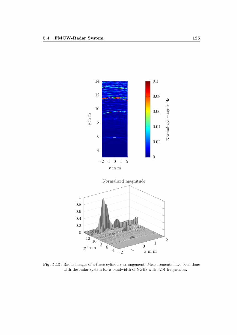
5.4. FMCW-Radar System 125
Nor
mal
ized
mag
nitu
de
yin
m
x in m
0
0.02
0.04
0.06
0.08
0.1
4
6
8
10
12
14
-2 -1 0 1 2
-2-1
01
2
46
810
120
0.2
0.4
0.6
0.8
1
Normalized magnitude
x in my in m
Fig. 5.15: Radar images of a three cylinders arrangement. Measurements have been done
with the radar system for a bandwidth of 5GHz with 3201 frequencies.

126 Chapter 5. FMCW-Radar Measurements
Nor
mal
ized
mag
nitu
de
yin
m
x in m
0
0.05
0.1
0.15
0.2
0.25
0.3
0.35
0.4
4
6
8
10
12
14
-2 -1 0 1 2
-2-1
01
2
46
810
120
0.2
0.4
0.6
0.8
1
Normalized magnitude
x in my in m
Fig. 5.16: Radar images of a three cylinders arrangement. Measurements have been done
with the radar system for a bandwidth of 5GHz and 30000 frequency points.

5.5. Conclusion 127
5.5 Conclusion
The results have shown that the proposed approach with fixed antennas could be aninteresting candidate for FOD detection without the need for mechanical scanning.Measurements have been done with a laboratory equipment as well as with a radarsystem. With the later the need for a short ramp duration have been pointed out.Further investigations have to be done with more adequate antennas, like antennasdirective in elevation and with a large beam-with in azimuth, in order to improvedetection capabilities. Reflect array antennas could be good candidates for thatparticular case. Additionally, studies are foreseen to obtain the bi-static responsewith the presented setup of the radar system as shown with the network analyzer.


Chapter 6
Conclusion and Outlook
6.1 Conclusion
In this work a valuable measurement system of 2D circular targets for imagingpurposes in the W-band has been presented. It has been tested on two metalliccylinders of 20mm and 8mm diameters, respectively, and on a dielectric cylinder of15mm. For this purpose, advantage has been taken of the short wavelength valueto build a small size system (0.7m × 0.6m). A post-processing scheme has beenproposed to correct misalignment errors as well as to reduce the noise. Hence, anoriginal filtering has been developed that does not require a-priori knowledge of thetarget. This is a key point in the perspective of the inversion of scattered fieldsfrom unknown objects. It has been successfully applied to the measured data of thetwo metallic and the dielectric cylinders and validated in simulations on irregularobjects under AWGN. Finally, the large metallic cylinder has been used as referencetarget for deriving the calibration coefficients and the smaller cylinders have beenused as test objects. Averaged values of the signal to noise ratio over W-band are15.4 dB and 10 dB for the large and the small metallic cylinders, respectively, and5.7 dB for the dielectric one.The measurement results have been used for the first time in the W-band forquantitative imaging purpose. The small metallic cylinder has been properlyretrieved with a high sigma value. This could be related to the benefit of usingmm-waves, that enhances the absolute resolution. Finally, the system sets the firstbasis for a more complex system capable to handle irregular objects.
A first measurement project in field has been started during this thesis to obtainresults for close range imaging based on a setup with two fixed antennas. Resultshave been pointed out that the presented approach could be a good candidate forthe detection of FOD with the already developed radar system in the W-band.
6.2 Outlook
A discussion on possible future work is given in the following.
• Based on the presented results the laboratory can establish a more complexmeasurement system which is needed to provide the multi-incidence and multi-view case to measure asymmetric objects. The calibration procedure devel-oped here can still be applied while using a metallic cylinder as the referencetarget.

130 Chapter 6. Conclusion and Outlook
• Further investigations are going to be done in the inversion of the data mea-sured for the larger metallic cylinder and the dielectric cylinder. Due to thegood agreement of the measured scattered fields of these targets with the an-alytic solution this should be possible with a marginal longer computationtime. The retrieved reconstructions obtained with the back-propagation setthe basis to estimate precisely the domain which has to be used for the quan-titative imaging. So far, no regularization scheme has been investigated. Inthe future, a multiplicative regularization is going to be implemented in anadditional module in FlexiMoM.
• Additional studies in order to simulate any polarization have been already pro-ceeded. Therefore, a module in FlexiMoM is under investigation to simulatealso the 2D-TE case.
• In general, the developed software FlexiMoM, due to its modular architec-ture, is going to be used as starting point to elaborate future direct and inverseelectromagnetic scattering problems.
• To create a database of “in-field” measurements for benchmarking algorithms,more adequate antennas have to be used. The standard gain horns shouldbe replaced by an antenna having a directive radiation pattern in elevationand an omni-directional radiation pattern in azimuth. For this purpose, areflect array antenna could be a good candidate due to the experience in theirdevelopment and realization of the laboratory.

Chapter 7
Resume in German and French
Due to the co-tutelle convention between the University of Nice - Sophia Antipolisand the University of Ulm it is supposed to provide a resume in German and English,which can be found in the following.
7.1 Zusammenfassung und Ausblick auf Deutsch
In der vorgestellten Arbeit wurde ein leistungsfähiges Messsystem für zweidi-mensionale kreisförmige Objekte mit dem Ziel der Rekonstruktion im W-Bandpräsentiert. Dieses wurde an zwei metallischen Zylindern mit Durchmessern vonjeweils 20mm und 8mm getestet sowie an einem dielektrischen Zylinder mit einemDurchmesser von 15mm. Aufgrund der kurzen Wellenlänge konnte ein kompaktesSystem (0.7m × 0.6m) entwickelt werden. Ein Signalverarbeitungsprozess wurdevorgestellt, um Justierungsfehler zu korrigieren und Rauschen zu reduzieren. Dabeiwurde eine neue Filtermethode entwickelt, welche keine Kenntnisse über das Objektvoraussetzt. Dieser kommt eine Schlüsselrolle zu, da zukünftig eine Rekonstruktiondurchgeführt werden soll mit Streufeldern von unbekannten Objekten. Die Methodewurde erfolgreich auf die Messdaten der zwei metallischen und des dielektrischenZylinders angewandt. Auch wurde sie in Simulationen von unsymmetrischenObjekten unter AWGN validiert. Schließlich wurde der große metallische Zylinderals Referenzobjekt verwendet, um die Kalibrationskoeffizienten zu ermitteln. Diezwei kleineren Zylinder dienten als Testobjekte. Durchschnittswerte des Signal-Rausch-Verhältnis über das W-Band sind 15.4 dB für den großen metallischenZylinder und 10 dB für den kleinen metallischen Zylinder sowie 5.7 dB für dendielektrischen Zylinder. Die Messergebnisse wurden erstmals im W-Band zurquantitativen Rekonstruktion verwendet. Der kleine metallische Zylinder wurdeerfolgreich mit einem hohen Konduktivitätswert rekonstruiert. Dies könnte imZusammenhang mit dem Nutzen vom mm-Wellen stehen, welche eine hohe absoluteAuflösung bereitstellen. Das vorgestellte System setzt die Basis für die zukünftigeEntwicklung eines komplexeren Messaufbaus, welcher genutzt werden soll, umunsymmetrische Objekte zu vermessen. Zusätzlich wurde eine erste Messkampagneim Feld gestartet, um Abbildungen im Nahbereich mit einem FMCW Radarsystemund zwei festen Empfängerpositionen zu erzielen. Die Ergebnisse zeigten, dass dervorgestellte Ansatz geeignet ist für die Detektierung von FOD im W-Band.
Im Folgenden wird ein Ausblick auf zukünftige Schwerpunkte gegeben. Basie-rend auf den präsentierten Ergebnissen kann das LEAT nun ein komplexeres Mess-

132 Chapter 7. Resume in German and French
system projektieren, welches benötigt wird, um unterschiedliche Empfängerpositio-nen mit unterschiedlichen Sendepositionen zu kombinieren. Dies ist notwendig, umunsymmetrische Objekte zu vermessen. Die entwickelte Kalibrationsmethode miteinem metallischen Zylinder als Referenzobjekt kann auch für diesen Fall angewen-det werden. Es werden Bestrebungen stattfinden, um die Messergebnisse von demgroßen metallischen Zylinder und dem dielektrischen Zylinder zur quantitativen Re-konstruktion zu verwenden. Durch die sehr gute Übereinstimmung der gemessenenStreufelder mit der analytischen Lösung sollte die Rekonstruktion mit nur unwe-sentlich längeren Berechnungszeiten möglich sein. Die Ergebnisse der qualitativenRekonstruktion setzen hierfür die Basis, um präzise den Bereich abzuschätzen, wel-cher für die quantitative Rekonstruktion verwendet werden wird. Bisher wurdennoch keine Regularisierungsalgorithmen eingesetzt. Zukünftig wird eine multiplika-tive Regularisierung in einem zusätzlichen Modul von FlexiMoM implementiertund untersucht werden. Zusätzliche Untersuchungen sind schon jetzt im Gange,um jede beliebige Polarisierung zu simulieren. Momentan wird die Implementie-rung eines zusätzlichen Moduls in FlexiMoM vorangetrieben, um den 2D-TE Fallzu berechnen. Generell wird FlexiMoM, dank des modularen Aufbaus, als Platt-form für zukünftige direkte und inverse elektromagnetische Streufeldberechnungendienen. Des weiteren soll eine Datenbank aufgebaut werden, welche Daten aus Feld-messungen mit dem FMCW Radarsystem enthält. Diese soll für die Validierung vonAlgorithmen herangezogen werden. Zusätzliche Messungen sollten mit Antennendurchgeführt werden, welche über ein direktives Strahlungsdiagramm in der Eleva-tion und ein omni-direktionales Strahlungsdiagramm im Azimuth verfügen. Für die-sen Zweck könnten Reflectarray-Antennen untersucht werden. In deren Entwicklungund Herstellung verfügt das MWT und das LEAT über langjährige Erfahrungen.

7.2. Résumé en français 133
7.2 Résumé en français
Durant la dernière décade, les radars millimétriques en bande W (75 − 110GHz)pour les applications civiles se sont largement développés, en partie grâce auxprogrès des circuits intégrés et à la possibilité de fabriquer des systèmes compactsà haute résolution. Les domaines d’applications sont nombreux et variés : secteurautomobile (radar d’aide à la conduite à 77GHz), aide au pilotage d’hélicoptères ouencore détection d’objets sur pistes d’aéroports (radars FOD à 77GHz ou 94GHz).Dans un premier temps ces systèmes ont été utilisés à des fins de détection.Cependant, leur maturité ainsi que les exigences accrues en termes d’application,orientent actuellement les recherches vers l’insertion de fonctions permettantl’identification.
Ainsi, des systèmes d’imagerie radar ont été développés, notamment à l’aided’imagerie SAR. Les premiers résultats obtenus avec cette imagerie qualitativesont très prometteurs car ils permettent de retrouver précisément la forme desobjets. Afin de reconstruire les propriétés électromagnétiques des objets, il est àprésent nécessaire de travailler de manière quantitative. De nombreux travaux ontété conduits en ondes centimétriques dans ce domaine, cependant aucun systèmed’imagerie quantitative n’existe, à notre connaissance, en gamme millimétrique.
L’objectif du travail présenté dans ce manuscrit est à la fois de poser lesbases d’un système d’imagerie quantitative en gamme millimétrique mais ausside le comparer à l’imagerie radar de systèmes développés en collaboration avec le«Institut für Mikrowellentechnik» de l’Université d’Ulm (Allemagne).Compte-tenu du peu de travaux dans le domaine de l’imagerie quantitative enbande millimétrique, la première étape consiste en la validation du processusde reconstruction sur des cibles canoniques. Nous avons choisi deux cylindresmétalliques et un cylindre diélectrique. Ce manuscrit décrit l’ensemble du processusau travers de six chapitres organisés comme suit.
Après un bref chapitre introductif, le chapitre 2 décrit les fondements théoriquesdes modèles utilisés à la fois pour le calcul du problème direct et du problèmeinverse. En gamme millimétrique de nombreux objets peuvent être vus en deux di-mensions (2D), par exemple les lignes à haute tension particulièrement dangereusespour les hélicoptères. Ainsi la modélisation du champ diffracté est développée pourle cas 2D-TM (Transverse Magnétique) et repose sur l’utilisation d’une Méthodedes Moments (MoM). Le logiciel ainsi développé est appelé FlexiMoM. C’est ceque nous appellerons modélisation du problème direct. Pour le cas particulier descylindres il existe de plus une solution analytique qui a été implémentée dans unlogiciel développé au laboratoire, appelé Escale. Ce dernier est dédié au calcul duchamp diffracté pour les cas où une solution analytique existe. Les comparaisonsentre la solution analytique et FlexiMoM valident la modélisation du problèmedirect. Le problème inverse est implémenté avec une méthode de gradient conjugué.

134 Chapter 7. Resume in German and French
Le troisième chapitre décrit le système de mesure. La difficulté de travailler engamme millimétrique est double. D’une part la faible valeur de la longueur d’ondedemande une meilleure précision mécanique. D’autre part, les performances desappareils de mesure, plancher de bruit et dynamique notamment, sont moindresqu’aux basses fréquences. Une spécificité supplémentaire est liée à l’activitéprincipale de la chambre anéchoide du LEAT qui est la mesure d’antennes. Ainsile système de mesure doit être compatible avec la mesure d’antennes, c’est à direfacile à installer et démonter.
Le système proposé tient compte de toutes ces contraintes et tire également par-tie des faibles valeurs de la longueur d’onde qui permet de concevoir un système dansun volume réduit. Ainsi, l’émetteur est placé à 400mm du système cible-récepteur.Afin que l’erreur d’alignement récepteur-cible soit constante et donc n’influence quela dynamique de mesure, la cible et le récepteur sont solidaires et placés, par l’inter-médiaire d’un mât, sur la tour de mesure. Le système ainsi conçu permet l’acquisitiondu champ diffracté en mono-incidence/multivues sur un cercle, ce qui correspondbien au cas modélisé 2D-TM. Cependant, la présence physique de l’émetteur em-pêche une mesure sur 360◦, la zone couverte est de 300◦ (φ = 30◦−330◦). La symétriedes cibles permet ensuite de passer facilement au cas multi-incidences/multivues parduplication fictive des émetteurs. Les trois fréquences de mesure sont les fréquenceslimites de la bande W (75GHz et 110GHz) et la fréquence centrale (92.5GHz).La comparaison des mesures brutes avec la solution exacte (Escale) met en évi-dence trois problèmes :
• un mauvais alignement entre l’émetteur et la cible qui se traduit par une phasedissymétrique,
• la présence de bruit,
• la nécessité de normaliser correctement les mesures et les simulations afin deprendre en compte la différence de puissance incidente dans les deux cas.
Le chapitre décrit ensuite l’ensemble des corrections apportées aux mesures etl’estimation des performances du système. La première étape est la correctiondu dés-alignement qui est dû au dé-centrage du mât par rapport au centre derotation de la tour. Elle est obtenue par optimisation à partir du grand cylindremétallique qui devient notre objet de calibrage. Le bruit de mesure est supprimépar filtrage. Ce bruit a une double cause. Il est lié d’une part à l’imprécision dupositionnement lors de deux rotations de la tour. Comme le champ diffracté estissu de la soustraction entre le champ sans cible (champ incident) et le champ aveccible (champ total), cette imprécision va générer du bruit. On montre en estimantson influence en simulations grâce à Escale, que ce dernier apparaît aux hautes«fréquences» du spectre issu de la transformation du champ E(φ). Il peut donc êtresupprimé par un filtre passe-bas. La seconde cause du bruit est liée aux appareils de
7.2. Résumé en français 135
mesure. Le bruit est d’autant plus important que les valeurs des champs incident ettotal sont proches. C’est pourquoi, pour nos cibles particulières testées, il apparaîtsurtout dans les premiers lobes. Une technique de filtrage originale qui ne nécessitepas de connaissance préalable des cibles sous test et fondée sur la détection depente, permet de supprimer les interférences du bruit avec le signal. Ce filtrage estaussi de type passe-bas. Finalement on montre que tout le bruit peut être éliminépar un filtre passe-bas dont la fréquence de coupure est déterminée par la détectionde pente des spectres.Enfin, la normalisation déjà utilisée au laboratoire à plus basse fréquence, etqui repose sur la corrélation des champs mesurés et simulés est appliquée. Lesrésultats ainsi corrigés présentent un SNR de 15.4 dB pour le grand cylindre (cequi constituera aussi notre limite haute du système), de 10 dB pour le plus petitcylindre métallique et de 5.7 dB pour le cylindre diélectrique.
Le chapitre 4 est consacré à l’imagerie réalisée à partir de ces mesures. Dansun premier temps, une imagerie qualitative, qui repose sur un algorithme de rétro-propagation est testée et donne d’excellents résultats puisque tous les contours descylindres sont reconstruits avec une précision d’une demi-longueur d’onde pour unseuillage à 3 dB.Dans un second temps, le petit cylindre est utilisé pour l’inversion. Son contour estlui aussi parfaitement reconstruit. Les caractéristiques diélectriques donnent unepermittivité relative proche de 1 et un sigma compris entre 77.37 S/m et 81.12 S/m.La dispersion des valeurs de sigma est liée au nombre de récepteurs utilisé pourl’inversion. Ces valeurs de la permittivité complexe sont caractéristiques d’unmétal. Cependant, bien que quantitatif, l’algorithme d’inversion utilisé ne permetpas de retrouver des valeurs de sigma réelles du métal (plusieurs MS/m). En d’autrestermes, nous pouvons identifier le métal mais nous ne sommes pas en mesure dedire de quel métal il s’agit. Cependant, cette dernière limitation n’est pas un freinpour les applications citées plus haut.
Enfin, des mesures sont initiées au chapitre 5 avec un système radar FM-CWbistatique développé en collaboration avec l’Université d’Ulm. Il est utilisé dansun cadre d’imagerie qualitative et repose sur l’utilisation de trois paramètres S
de la mesure (S11, S12 ou S21 et S22). Dans un premier temps, les mesures sontconduites avec un analyseur de réseau vectoriel pour valider le concept. DifférentsFOD ont été détectés avec succès avec toute la bande passante de la bande W,puis avec une bande passante réduite de 5GHz, qui correspond à la bande passantemaximale de notre radar. Les mesures radar montrent les paramètres S11 et S22sont exploitables et que les FOD peuvent être trouvés à condition que l’objet soitdans la zone d’intersection des champs de vision des deux antennes du radar.L’exploitation du paramètre S21 et/ou S12 reste problématique et les recherchesdoivent être poursuivies dans ce domaine.

136 Chapter 7. Resume in German and French
L’ensemble des résultats obtenus valident le processus développé pour d’imageriequantitative en gamme millimétrique. Les recherches doivent être poursuivies aussibien en mesure qu’en modélisation. D’une part le système de mesure doit évoluervers un vrai système multi-incidences/multivues. Grâce aux résultats obtenus avecnotre système simplifié, ce dernier a pu être dimensionné et nous espérons des fondspour pouvoir l’installer. D’autre part, le cas 2D-TE doit être implémenté afin depouvoir traiter un objet 2D quelconque dans n’importe quelle polarisation.Enfin, les mesures à partir de systèmes radar réels doivent être poursuivies, enparticulier pour rendre exploitables les mesures des coefficients de transmission. Cesdernières sont indispensable si l’on veut un jour appliquer les algorithmes d’inversionà des mesures issues de systèmes radar.
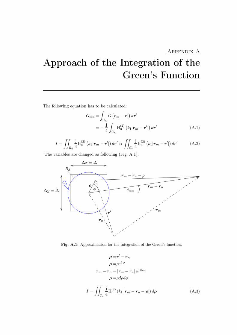
Appendix A
Approach of the Integration of the
Green’s Function
The following equation has to be calculated:
Gmn =
∫
Cn
G(rm − r′
)dr′
=− j
4
∫
Cn
H(2)0
(k1|rm − r′|
)dr′ (A.1)
I =
∫∫
Rd
j
4H(2)
0
(k1|rm − r′|
)dr′ ≈
∫∫
Ca
j
4H(2)
0
(k1|rm − r′|
)dr′ (A.2)
The variables are changed as following (Fig. A.1):
∆x = ∆
Rd
rm − rn − ρ
Ca
∆y = ∆rm − rnρ
φ φnm
rmr′
rn
Fig. A.1: Approximation for the integration of the Green’s function.
ρ =r′ − rn
ρ =ρe jφ
rm − rn = |rm − rn| e jφnm
ρ =ρdρdφ.
I =
∫∫
Ca
j
4H(2)
0 (k1 |rm − rn − ρ|) dρ (A.3)

138 Appendix A. Approach of the Integration of the Green’s Function
A.1 Self Element Case, n = m, Diagonal Matrix Ele-
ments
I =
∫∫
Ca
j
4H(2)
0 (k1ρ) dρ
=
∫ 2π
0
∫ R
0
j
4H(2)
0 (k1ρ) ρdρdφ
=jπ
2
∫ R
0H(2)
0 (k1ρ) ρdρ (A.4)
=jπ
2
1
k1
∫ R
0H(2)
0 (k1ρ)k1ρdρ
Integration by substitution
t =k1ρ⇒ dt
dρ= k1 ⇒ dρ =
dt
k1
=jπ
2
1
k1
∫ t=k1R
t=0H(2)
0 (t)tdt
k1
=jπ
2
1
k21
[H(2)
1 (t)t]t=k1R
t=0
=jπ
2
1
k21
(H(2)
1 (k1R)k1R− H(2)1 (t)t|t→0
)
One has to calculate: H(2)1 (t)t|t→0
tH(2)1 (t)|t→0 =t [J1(t)− jY1(t)] |t→0
After [110]:
Yn(z) =−(12z)−n
π
n−1∑
k=0
(n− k − 1)!
k!
(1
4z2)k
+2
πln
(1
2z
)Jn(z)
−(12z)n
π
∞∑
k=0
[ψ(k + 1) + ψ(n + k + 1)]
(−1
4z2)k
k!(n+ k)!
ψ(1) =− γ
ψ(n) =− γ +
n−1∑
k=1
k−1(n ≤ 2)

A.1. Self Element Case, n = m, Diagonal Matrix Elements 139
Y1(z) =−(12z)−1
π
1−1∑
k=0
(1− k − 1)!
k!
(1
4z2)k
+2
πln
(1
2z
)J1(z)
−(12z)1
π
∞∑
k=0
[ψ(k + 1) + ψ(1 + k + 1)]
(−1
4z2)k
k!(1 + k)!
Y1(z) =−(12z)−1
π
1−1∑
k=0
(1− k − 1)!
k!
(1
4z2)k
+2
πln
(1
2z
)J1(z)
−(12z)1
π
∞∑
k=0
−γ +
(k+1)−1∑
n=1
n−1
+
−γ +
(1+k+1)−1∑
n=1
n−1
(−1
4z2)k
k!(1 + k)!
Y1(z) =− 2
zπ
0!
0!
(1
4z2)0
+2
π
[ln(
(1
2
)+ ln(z)
]J1(z)
− z
2π
∞∑
k=0
[(−γ +
k∑
n=1
n−1
)+
(−γ +
1+k∑
n=1
n−1
)] (−1
4z2)k
k!(1 + k)!
Y1(z) ≈− 2
zπ
+2
π
[ln
(1
2
)+ ln(z)
]J1(z)
−z(Cz2
)︸ ︷︷ ︸
1
tH(2)1 (t)|t→0 =t [J1(t)− jY1(t)] |t→0
=tJ1(t)|t→0 − t jY1(t)|t→0
≈0− j t
(− 2
tπ+
2
π
[ln
(1
2
)+ ln(t)
]J1(t)− t
(Ct2))
|t→0
=j2
π
I =jπ
2
1
k21
(H(2)
1 (k1R)k1R−(j2
π
))(A.5)
1This gives a first approximation of first order to calculate the equations (2.47) and (2.48).

140 Appendix A. Approach of the Integration of the Green’s Function
A.2 General Case, n 6= m, Non-diagonal Matrix Ele-
ments
With the addition theorem [111] one can write:
H(2)0 (k1 |rm − rn − ρ|) =
∞∑
q=−∞H(2)
q (k1 |rm − rn|) Jq (k1ρ) ej q(φ−φnm) (A.6)
since ρ < |rm − rn|
The integral becomes:
I ≈ j
4
∞∑
q=−∞H(2)
q (k1 |rm − rn|)∫ R
0Jq (k1ρ) ρ dρ
∫ 2π
0e j q(φ−φnm)dφ (A.7)
The last term in the sum gets:
∫ 2π
0e j q(φ−φnm)dφ =
{0, if q 6= 0
2π, if q = 0
Only the term q = 0 is conserved.∫xλ+1Zλ(z)dx = zλ+1Zλ+1(x)
In the following, one has to solve:∫ R
0J0 (k1ρ) ρdρ (A.8)
∫ R
0J0 (k1ρ) ρdρ =
1
k1
∫ R
0J0 (k1ρ) k1ρdρ
Using integration by substitution
t = k1ρ⇒ dt
dρ= k1 ⇒ dρ =
dt
k1
=1
k1
∫ t=k1R
t=0J0(t)t
dt
k1
=1
k21
∫ t=k1R
t=0J0(t)tdt
=1
k21[J1(t)t]
t=k1Rt=0
=1
k21(k1RJ1(k1R)− tJ1(t)|t→0)
with J1(x)|x→0 = 0
=R
k1J1 (k1R)

A.2. General Case, n 6= m, Non-diagonal Matrix Elements 141
I =
∫∫
Ca
j
4H(2)
0 (k1 |rm − rn − ρ|) dρ
=j
42π
R
k1J1 (Rk1)H(2)
0 (k1 |rm − rn|)
I =jπR
2k1H(2)
0 (k1 |rm − rn|) J1 (Rk1) (A.9)


Appendix B
Approach for the Integration over
a Squared Disc with an Optimal
Circular Disc
B.1 Demonstration
������������������������������������������������������������������������������
������������������������������������������������������������������������������
������������������������������������������������������������������������������������������������������������������������
������������������������������������������������������������������������������������������������������������������������
∆y = ∆
R
Rd
Ca
∆x = ∆
Fig. B.1: Approximate integration over a squared cell over an optimal circular disc.
One can show that each polynomial P (x, y) of order three 1:
P (x, y) = c0 + c1x+ c2y + c3x2 + c4xy + c5y
2 + c6x3 + c7x
2y + c8xy2 + c9y
3
fulfills∫∫
Rd
P (x, y)dxdy =3
π
∫∫
Ca
P (x, y)dxdy (B.1)
assumed that the rectangle is square and its side length and the radius of the circleR are related by
R =∆√3. (B.2)
1Second approximation of order 3 to calculate the equations (2.47) and (2.48)

144Appendix B. Approach for the Integration over a Squared Disc with an
Optimal Circular Disc
∫∫
Rd
P (x, y)dxdy =
∫ ∆
2
−∆
2
∫ ∆
2
−∆
2
c0 + c1x+ c2y + c3x2 + c4xy + c5y
2
+ c6x3 + c7x
2y + c8xy2 + c9y
3dxdy (B.3)
∫∫
Ca
P (x, y)dxdy =
∫ 2π
0
∫ R
0c0 + c1x+ c2y + c3x
2 + c4xy + c5y2
+ c6x3 + c7x
2y + c8xy2 + c9y
3rdrdφ (B.4)
∫ ∆
2
−∆
2
∫ ∆
2
−∆
2
P (x, y)dxdy =c0∆2 + c3
∆4
12+ c5
∆4
12∫ 2π
0
∫ R
0P (x, y)rdrdφ =c0πR
2 + c31
4R4π + c5
1
4R4π
∫ ∆
2
−∆
2
∫ ∆
2
−∆
2
P (x, y)dxdy = C∫ 2π
0
∫ R
0P (x, y)rdrdφ
⇒ C =∆2
πR2et R =
∆√3
⇒ C =3
π
One has to show that the algebraical expression to integrate equation (A.8) andequation (A.4) are polynomials of order three to apply the following approximation.
∫ (xi+∆
2)
(xi−∆
2)
∫ (xi+∆
2)
(xi−∆
2)
J0 (k1ρ)︸ ︷︷ ︸P1(x,y)
dx′dy′ =C∫ R
0
∫ 2π
0J0 (k1ρ) ρdρdφ
∫ (xi+∆
2)
(xi−∆
2)
∫ (xi+∆
2)
(xi−∆
2)
H(2)0 (k1ρ)︸ ︷︷ ︸P2(x,y)
dx′dy′ =C∫ R
0
∫ 2π
0H(2)
0 (k1ρ) ρdρdφ
(B.5)
with R =∆√3
C =3
π
ρ =√x′2 + y′2
with the substitutions:
x′ =ρ cos(φ)
y′ =ρ sin(φ)
dx′dy′ =ρdρdφ
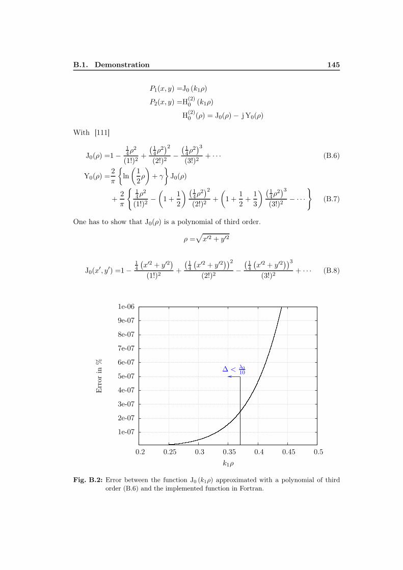
B.1. Demonstration 145
P1(x, y) =J0 (k1ρ)
P2(x, y) =H(2)0 (k1ρ)
H(2)0 (ρ) = J0(ρ)− jY0(ρ)
With [111]
J0(ρ) =1−14ρ
2
(1!)2+
(14ρ
2)2
(2!)2−(14ρ
2)3
(3!)2+ · · · (B.6)
Y0(ρ) =2
π
{ln
(1
2ρ
)+ γ
}J0(ρ)
+2
π
{14ρ
2
(1!)2−(1 +
1
2
) (14ρ
2)2
(2!)2+
(1 +
1
2+
1
3
) (14ρ
2)3
(3!)2− · · ·
}(B.7)
One has to show that J0(ρ) is a polynomial of third order.
ρ =√x′2 + y′2
J0(x′, y′) =1−
14
(x′2 + y′2
)
(1!)2+
(14
(x′2 + y′2
))2
(2!)2−(14
(x′2 + y′2
))3
(3!)2+ · · · (B.8)
1e-07
2e-07
3e-07
4e-07
5e-07
6e-07
7e-07
8e-07
9e-07
1e-06
0.2 0.25 0.3 0.35 0.4 0.45 0.5
Err
orin
%
k1ρ
∆ < λ0
10
Fig. B.2: Error between the function J0 (k1ρ) approximated with a polynomial of third
order (B.6) and the implemented function in Fortran.
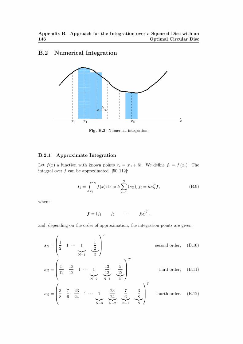
146Appendix B. Approach for the Integration over a Squared Disc with an
Optimal Circular Disc
B.2 Numerical Integration
������������������������������������������������������������
������������������������������������������������������������
h
x0 x1 xN x
Fig. B.3: Numerical integration.
B.2.1 Approximate Integration
Let f(x) a function with known points xi = x0 + ih. We define fi = f (xi). Theintegral over f can be approximated [50, 112]:
I1 =
∫ xN
x1
f(x) dx ≈ hN∑
i=1
(sN)i fi = hsTNf , (B.9)
where
f = (f1 f2 · · · fN)T ,
and, depending on the order of approximation, the integration points are given:
sN =
1
21 · · · 1
︸︷︷︸N−1
1
2︸︷︷︸N
T
second order, (B.10)
sN =
5
12
13
121 · · · 1
︸︷︷︸N−2
13
12︸︷︷︸N−1
5
12︸︷︷︸N
T
third order, (B.11)
sN =
3
8
7
6
23
241 · · · 1
︸︷︷︸N−3
23
24︸︷︷︸N−2
7
6︸︷︷︸N−1
3
8︸︷︷︸N
T
fourth order. (B.12)

B.3. Chosen Approach versus Numerical Integration 147
B.2.2 Approximate Double Integration
Let f(x, y) a function with known points (xi, yi) where xi = x0 + ihx andyj = y0 + jhy . We define fij = f(xi, yj). The double integral over f can be ap-proximated:
I2 =
∫∫ (xN,yM)
(x1,y1)f(x, y) dxdy =
∫ yM
y1
(∫ xN
x1
f(x, y) dx
)dy
≈∫ yM
y1
(hx
N∑
i=1
(sN)i fij
)dy
≈ hxhy
N∑
i=1
M∑
j=1
(sN)i (sM)j fij = hxhysTNFsM (B.13)
where the elements of the matrix F , which has the dimension N×M, are the valuesof fij. The integral I2 can also be written as:
I2 ≈ hxhy
N∑
i=1
M∑
j=1
(dNM)ij fij (B.14)
where the weights (dNM)ij = (sN)i (sM)j are the elements of the matrix DNM, whichhas the dimension N × M, given by:
DNM = sNsT
M. (B.15)
B.3 Comparison between Chosen Approach and Numer-
ical Integration
The equations (2.47) and (2.48) have been implemented in FlexiMoM. Also thenumerical integration presented in (2.41) and (2.43) is choice-able. In order tocalculate the integral for the case n = m, N and M have to be even-numbers. If thisis not the case one would be in a singularity of H(0).
B.3.1 Wavelength in the Order of Meters
The difference between the results obtained for a cell size of λ0/10 and λ0/20 can beexplained as following: smaller the cell is closer are the results for the approxima-tion and for the numerical integration to the exact solution. That’s why also thedifference between both is smaller.

148Appendix B. Approach for the Integration over a Squared Disc with an
Optimal Circular Disc
Parameter First case Second case Unit
Frequency f = 1 GHz
Areax = −1.5 · · · 1.5 m
y = −1.5 · · · 1.5 m
∆x 0.03 = λ0
10 0.015 = λ0
20 m
∆y 0.03 = λ0
10 0.015 = λ0
20 m
Tab. B.1: Chosen parameters to compare numerical integration with chosen approach.
20log(r
elat
ive
erro
r)
yin
m
x in m
-110-100-90-80-70-60-50
-1.5
-1
-0.5
0
0.5
1
1.5
-1.5 -1 -0.5 0 0.5 1 1.5
Fig. B.4: Error between approach and numerical integration for N=10 and ∆ = λ0
10.
-130-120-110-100-90-80-70-60-50-40
-0.5 0 0.5 1 1.5
20log(r
elat
ive
erro
r)
x in m
∆ = λ0/10; N=10∆ = λ0/20; N=10
∆ = λ0/10; N=100∆ = λ0/20; N=100
Fig. B.5: Error as function of N.
Time in CPU secondsλ0
10λ0
20
Approximation 0.012001 0.040002
N = 10 1.8841 7.5845
N = 100 88.210 359.91
Tab. B.2: Differences in computation time between the approach and the numerical inte-
gration.

B.3. Chosen Approach versus Numerical Integration 149
B.3.2 Wavelength in the Order of Millimeters
Parameter First case Second case Unit
Frequency f = 100 GHz
Areax = −0.015 · · · 0.015 m
y = −0.015 · · · 0.015 m
∆x 0.0003 = λ0
10 0.00015 = λ0
20 m
∆y 0.0003 = λ0
10 0.00015 = λ0
20 m
Tab. B.3: Chosen parameters to compare numerical integration with chosen approach.
20log(r
elat
ive
erro
r)
yin
mm
x in mm
-110-100-90-80-70-60-50
-1.5
-1
-0.5
0
0.5
1
1.5
-1.5 -1 -0.5 0 0.5 1 1.5
Fig. B.6: Error between approach and numerical integration for N=10 and ∆ = λ0
10.
-130-120-110-100-90-80-70-60-50-40
-0.005 0 0.005 0.01 0.015
20log(r
elat
ive
erro
r)
x in m
∆ = λ0/10; N=10∆ = λ0/20; N=10
∆ = λ0/10; N=100∆ = λ0/20; N=100
Fig. B.7: Error as function of N.


Appendix C
Additional Scattered Field
Measurements
In the main body of the manuscript only measurements have been shown for thecenter frequency of 92.5GHz. In the following, results are presented for 75GHz
and 110GHz. The results have been obtained by using the open-ended waveguideas emitting antenna and the standard gain horn as receiver.
Firstly, the results are plotted for 75GHz: the measured incident field (Fig. C.1),the measured total field for the metallic cylinders with D = 20mm (Fig. C.2) andD = 8mm (Fig. C.4), respectively, as well as for the dielectric cylinder (Fig. C.6).Out of these results the scattered fields are extracted (see Fig. C.3, Fig. C.5 andFig. C.7) and compared with the analytic solution. Therefore, the amplitude ofthe measured and simulated scattered fields have been normalized with respect totheir maxima. In simulation with Escale a diameter of 15.4mm, an εr = 2.49 anda σ = 0.1243 S/m have been taken to characterize the dielectric cylinder.
Additionally, measured fields for 110GHz are visualized: the measured incidentfield (C.8), the measured total field for the metallic cylinders with D = 20mm
(Fig. C.9) and D = 8mm (Fig. C.11), respectively, and for the dielectric cylinder(Fig. C.13). The extracted scattered fields from measurements are compared withsimulations in Fig. C.10, Fig. C.12 and Fig. C.14.

152 Appendix C. Additional Scattered Field Measurements
-90-80-70-60-50-40-30-20-10
0
60 120 180 240 300
Am
plitud
ein
dB
φ in degree
-4-3-2-101234
60 120 180 240 300
Pha
sein
rad
φ in degree
-700-600-500-400-300-200-100
0100
60 120 180 240 300
Unw
.ph
ase
inrad
φ in degree
Fig. C.1: Measured incident field for f = 75GHz in amplitude (top), phase (middle) and
unwrapped phase (bottom).

153
-90-80-70-60-50-40-30-20-10
0
60 120 180 240 300
Am
plitud
ein
dB
φ in degree
-4-3-2-101234
60 120 180 240 300
Pha
sein
rad
φ in degree
-120-100-80-60-40-20
020
60 120 180 240 300
Unw
.ph
ase
inrad
φ in degree
Fig. C.2: Measured total field with metallic cylinder, D = 20mm, for f = 75GHz in
amplitude (top), phase (middle) and unwrapped phase (bottom).
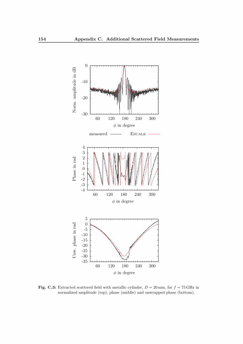
154 Appendix C. Additional Scattered Field Measurements
-30
-20
-10
0
60 120 180 240 300
Nor
m.
ampl
itud
ein
dB
φ in degree
measured Escale
-4-3-2-101234
60 120 180 240 300
Pha
sein
rad
φ in degree
-35-30-25-20-15-10-505
60 120 180 240 300
Unw
.ph
ase
inrad
φ in degree
Fig. C.3: Extracted scattered field with metallic cylinder, D = 20mm, for f = 75GHz in
normalized amplitude (top), phase (middle) and unwrapped phase (bottom).

155
-90-80-70-60-50-40-30-20-10
0
60 120 180 240 300
Am
plitud
ein
dB
φ in degree
-4-3-2-101234
60 120 180 240 300
Pha
sein
rad
φ in degree
-140-120-100-80-60-40-20
020
60 120 180 240 300
Unw
.ph
ase
inrad
φ in degree
Fig. C.4: Measured total field with metallic cylinder, D = 8mm, for f = 75GHz in am-
plitude (top), phase (middle) and unwrapped phase (bottom).

156 Appendix C. Additional Scattered Field Measurements
-30
-20
-10
0
60 120 180 240 300
Nor
m.
ampl
itud
ein
dB
φ in degree
measured Escale
-4-3-2-101234
60 120 180 240 300
Pha
sein
rad
φ in degree
-16-14-12-10-8-6-4-202
60 120 180 240 300
Unw
.ph
ase
inrad
φ in degree
Fig. C.5: Extracted scattered field with metallic cylinder, D = 8mm, for f = 75GHz in
normalized amplitude (top), phase (middle) and unwrapped phase (bottom).

157
-90-80-70-60-50-40-30-20-10
0
60 120 180 240 300
Am
plitud
ein
dB
φ in degree
-4-3-2-101234
60 120 180 240 300
Pha
sein
rad
φ in degree
-160-140-120-100-80-60-40-20
020
60 120 180 240 300
Unw
.ph
ase
inrad
φ in degree
Fig. C.6: Measured total field with dielectric cylinder for f = 75GHz in amplitude (top),
phase (middle) and unwrapped phase (bottom).
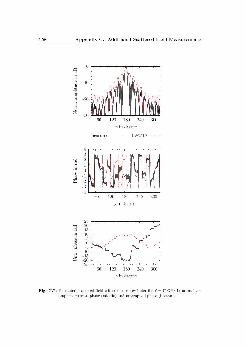
158 Appendix C. Additional Scattered Field Measurements
-30
-20
-10
0
60 120 180 240 300
Nor
m.
ampl
itud
ein
dB
φ in degree
measured Escale
-4-3-2-101234
60 120 180 240 300
Pha
sein
rad
φ in degree
-25-20-15-10-505
10152025
60 120 180 240 300
Unw
.ph
ase
inrad
φ in degree
Fig. C.7: Extracted scattered field with dielectric cylinder for f = 75GHz in normalized
amplitude (top), phase (middle) and unwrapped phase (bottom).

159
-90-80-70-60-50-40-30-20-10
0
60 120 180 240 300
Am
plitud
ein
dB
φ in degree
-4-3-2-101234
60 120 180 240 300
Pha
sein
rad
φ in degree
-500
-400
-300
-200
-100
0
100
60 120 180 240 300
Unw
.ph
ase
inrad
φ in degree
Fig. C.8: Measured incident field for f = 110GHz in amplitude (top), phase (middle) and
unwrapped phase (bottom).

160 Appendix C. Additional Scattered Field Measurements
-90-80-70-60-50-40-30-20-10
0
60 120 180 240 300
Am
plitud
ein
dB
φ in degree
-4-3-2-101234
60 120 180 240 300
Pha
sein
rad
φ in degree
-120-100-80-60-40-20
020
60 120 180 240 300
Unw
.ph
ase
inrad
φ in degree
Fig. C.9: Measured total field with metallic cylinder, D = 20mm, for f = 110GHz in
amplitude (top), phase (middle) and unwrapped phase (bottom).
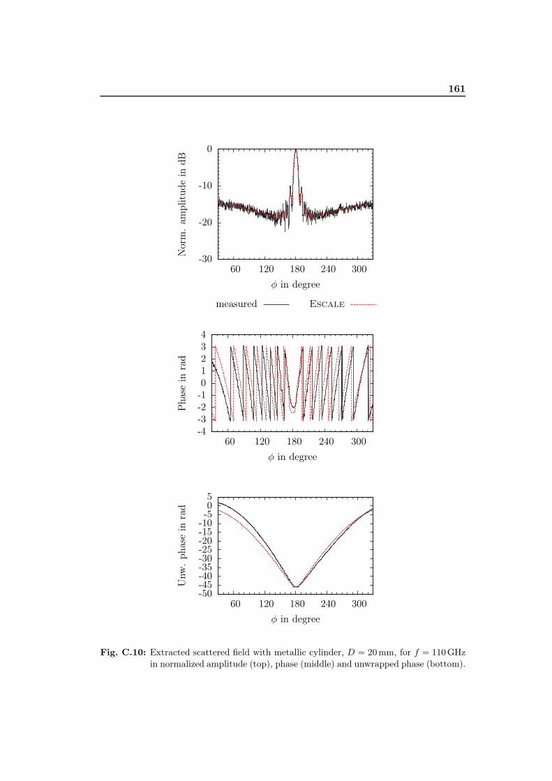
161
-30
-20
-10
0
60 120 180 240 300
Nor
m.
ampl
itud
ein
dB
φ in degree
measured Escale
-4-3-2-101234
60 120 180 240 300
Pha
sein
rad
φ in degree
-50-45-40-35-30-25-20-15-10-505
60 120 180 240 300
Unw
.ph
ase
inrad
φ in degree
Fig. C.10: Extracted scattered field with metallic cylinder, D = 20mm, for f = 110GHz
in normalized amplitude (top), phase (middle) and unwrapped phase (bottom).
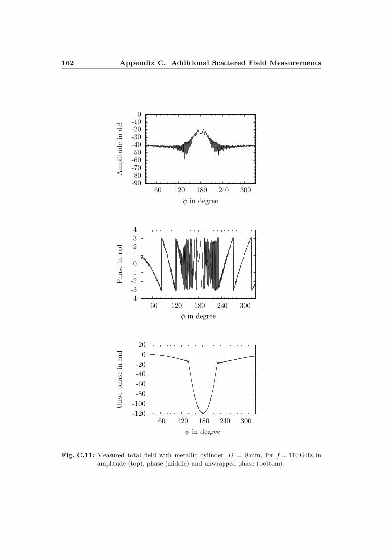
162 Appendix C. Additional Scattered Field Measurements
-90-80-70-60-50-40-30-20-10
0
60 120 180 240 300
Am
plitud
ein
dB
φ in degree
-4-3-2-101234
60 120 180 240 300
Pha
sein
rad
φ in degree
-120-100-80-60-40-20
020
60 120 180 240 300
Unw
.ph
ase
inrad
φ in degree
Fig. C.11: Measured total field with metallic cylinder, D = 8mm, for f = 110GHz in
amplitude (top), phase (middle) and unwrapped phase (bottom).
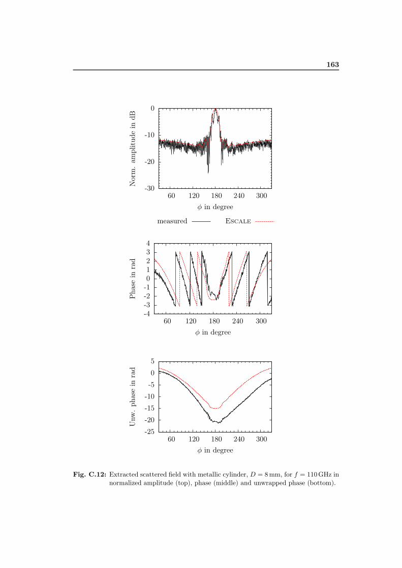
163
-30
-20
-10
0
60 120 180 240 300
Nor
m.
ampl
itud
ein
dB
φ in degree
measured Escale
-4-3-2-101234
60 120 180 240 300
Pha
sein
rad
φ in degree
-25
-20
-15
-10
-5
0
5
60 120 180 240 300
Unw
.ph
ase
inrad
φ in degree
Fig. C.12: Extracted scattered field with metallic cylinder, D = 8mm, for f = 110GHz in
normalized amplitude (top), phase (middle) and unwrapped phase (bottom).
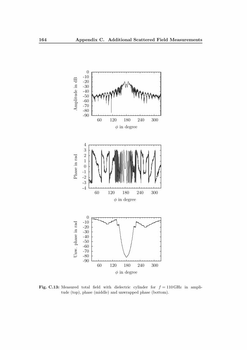
164 Appendix C. Additional Scattered Field Measurements
-90-80-70-60-50-40-30-20-10
0
60 120 180 240 300
Am
plitud
ein
dB
φ in degree
-4-3-2-101234
60 120 180 240 300
Pha
sein
rad
φ in degree
-90-80-70-60-50-40-30-20-10
0
60 120 180 240 300
Unw
.ph
ase
inrad
φ in degree
Fig. C.13: Measured total field with dielectric cylinder for f = 110GHz in ampli-
tude (top), phase (middle) and unwrapped phase (bottom).

165
-30
-20
-10
0
60 120 180 240 300
Nor
m.
ampl
itud
ein
dB
φ in degree
measured Escale
-4-3-2-101234
60 120 180 240 300
Pha
sein
rad
φ in degree
-25
-20
-15
-10
-5
0
5
60 120 180 240 300
Unw
.ph
ase
inrad
φ in degree
Fig. C.14: Extracted scattered field with dielectric cylinder for f = 110GHz in normalized
amplitude (top), phase (middle) and unwrapped phase (bottom).


Bibliography
[1] W. Mayer, A. Gronau, W. Menzel, and H. Leier, “A Compact 24 GHz Sensorfor Beam-Forming and Imaging,” in 9th International Conference on Control,
Automation, Robotics and Vision (ICARCV 2006). IEEE, Dec. 2006, pp.1–6.Referenced on page: 1, 1
[2] B. Michael, W. Menzel, and A. Gronau, “A real-time close-range imagingsystem with fixed antennas,” IEEE Transactions on Microwave Theory and
Techniques, vol. 48, no. 12, pp. 2736–2741, Dec. 2000.Referenced on page: 1, 1, 28, 108, 109
[3] M. Andres, P. Feil, and W. Menzel, “3D-scattering center detection of auto-motive targets using 77 GHz UWB radar sensors,” in 6th European Conference
on Antennas and Propagation (EUCAP 2012). IEEE, Mar. 2012, pp. 3690–3693.Referenced on page: 1
[4] C. Migliaccio, B. D. Nguyen, C. Pichot, N. Yonemoto, K. Yamamoto, K. Ya-mada, H. Nasui, W. Mayer, A. Gronau, and W. Menzel, “Millimeter-WaveRadar for Rescue Helicopters,” in 9th International Conference on Control,
Automation, Robotics and Vision (ICARCV 2006). IEEE, Dec. 2006, pp.1–6.Referenced on page: 1, 1
[5] H. Essen, S. Boehmsdorff, G. Biegel, and A. Wahlen, “On the scattering mech-anism of power lines at millimeter-waves,” IEEE Transactions on Geoscience
and Remote Sensing, vol. 40, no. 9, pp. 1895–1903, Sep. 2002.Referenced on page: 1, 1
[6] K. Sarabandi and M. Park, “Extraction of power line maps from millimeter-wave polarimetric SAR images,” IEEE Transactions on Antennas and Propa-
gation, vol. 48, no. 12, pp. 1802–1809, Dec. 2000.Referenced on page: 1, 1
[7] ——, “A radar cross-section model for power lines at millimeter-wave frequen-cies,” IEEE Transactions on Antennas and Propagation, vol. 51, no. 9, pp.2353–2360, Sep. 2003.Referenced on page: 1, 1
[8] P. Feil, W. Menzel, T. P. Nguyen, C. Pichot, and C. Migliaccio, “Foreignobjects debris detection (FOD) on airport runways using a broadband 78 GHzsensor,” in European Radar Conference (EURAD 2008). IEEE, Oct. 2008,pp. 451–454.Referenced on page: 1, 1, 1, 108

168 Bibliography
[9] M. R. Hajihashemi and M. El-Shenawee, “The Level Set Shape ReconstructionAlgorithm Applied to 2D PEC Targets Hidden Behind a Wall,” Progress In
Electromagnetics Research B, vol. 25, pp. 131–154, 2010.Referenced on page: 1
[10] A. Cresp, I. Aliferis, M. J. Yedlin, C. Pichot, and J.-Y. Dauvignac, “Investi-gation of time-reversal processing for surface-penetrating radar detection in amultiple-target configuration,” in European Radar Conference (EURAD 2008).IEEE, Oct. 2008, pp. 144–147.Referenced on page: 1, 2
[11] M. Yedlin, A. Cresp, C. Pichot, I. Aliferis, J.-Y. Dauvignac, S. Gaffet, andG. Sénéchal, “Ultra-wideband microwave imaging of heterogeneities,” Journal
of Applied Geophysics, vol. 68, no. 1, pp. 17–25, May 2009.Referenced on page: 1, 2
[12] M. Leib, E. Schmitt, A. Gronau, J. Dederer, B. Schleicher, H. Schumacher,and W. Menzel, “A Compact Ultra-wideband Radar for Medical Applications,”Frequenz, vol. 63, no. 1-2, pp. 2–8, Feb. 2009.Referenced on page: 1
[13] D. L. McMakin, D. M. Sheen, J. W. Griffin, N. B. Valentine, and W. M.Lechelt, “Personnel and mail screening with millimeter waves,” in Defense
and Security Symposium 2005, vol. 5778, no. 1. The International Societyfor Optical Engineering., Aug. 2005, pp. 160–168.Referenced on page: 1
[14] O. M. Bucci, L. Crocco, T. Isernia, and V. Pascazio, “Inverse scattering prob-lems with multifrequency data: reconstruction capabilities and solution strate-gies,” IEEE Transactions on Geoscience and Remote Sensing, vol. 38, no. 4,pp. 1749–1756, Jul. 2000.Referenced on page: 1
[15] M. R. Hajihashemi and M. El-Shenawee, “Shape Reconstruction Using theLevel Set Method for Microwave Applications,” Antennas and Wireless Prop-
agation Letters, IEEE, vol. 7, pp. 92–96, 2008.Referenced on page: 1
[16] M. El-Shenawee, O. Dorn, and M. Moscoso, “An Adjoint-Field Technique forShape Reconstruction of 3-D Penetrable Object Immersed in Lossy Medium,”IEEE Transactions on Antennas and Propagation, vol. 57, no. 2, pp. 520–534,Feb. 2009.Referenced on page: 1
[17] K. Belkebir, J. M. Elissalt, J. M. Geffrin, and C. Pichot, “Newton-Kantorovichand Modified Gradient - Inversion Algorithms Applied to Ipswich Data,” An-
tennas and Propagation Magazine, vol. 38, no. 3, pp. 41–44, Jun. 1996.Referenced on page: 1, 1, 35

Bibliography 169
[18] D. A. Woten, M. R. Hajihashemi, A. M. Hassan, and M. El-Shenawee, “Exper-imental Microwave Validation of Level Set Reconstruction Algorithm,” IEEE
Transactions on Antennas and Propagation, vol. 58, no. 1, pp. 230–233, Jan.2010.Referenced on page: 1
[19] P. Lobel, R. E. Kleinman, C. Pichot, L. Blanc-Féraud, and M. Barlaud,“Conjugate-Gradient Method for Solving Inverse Scattering with Experimen-tal Data,” Antennas and Propagation Magazine, vol. 38, no. 3, pp. 48–51, Jun.1996.Referenced on page: 1, 1, 25, 30, 35, 66, 98, 101, 104, 106
[20] P. M. van den Berg, M. G. Cote, and R. E. Kleinman, “”Blind” shape re-construction from experimental data,” IEEE Transactions on Antennas and
Propagation, vol. 43, no. 12, pp. 1389–1396, Dec. 1995.Referenced on page: 1, 35
[21] B. Gustafson, “Microwave analog to light scattering measurements: A modernimplementation of a proven method to achieve precise control,” Journal of
Quantitative Spectroscopy and Radiative Transfer, vol. 55, no. 5, pp. 663–672,May 1996.Referenced on page: 1, 36
[22] Y. Xu, “A generalized multiparticle Mie-solution: further experimental verifi-cation,” Journal of Quantitative Spectroscopy and Radiative Transfer, vol. 70,no. 4-6, pp. 395–419, Aug. 2001.Referenced on page: 1
[23] J. M. Geffrin and P. Sabouroux, “Continuing with the Fresnel database: ex-perimental setup and improvements in 3D scattering measurements,” Inverse
Problems, vol. 25, no. 2, Feb. 2009.Referenced on page: 1, 36
[24] J.-M. Geffrin, P. Sabouroux, and C. Eyraud, “Free space experimental scatter-ing database continuation: experimental set-up and measurement precision,”Inverse Problems, vol. 21, no. 6, pp. S117–S130, Dec. 2005.Referenced on page: 1, 36, 36
[25] M. G. Cote, “Automated swept-angle bistatic scattering measurements usingcontinuous wave radar,” IEEE Transactions on Instrumentation and Measure-
ment, vol. 41, no. 2, pp. 185–192, Apr. 1992.Referenced on page: 1, 35
[26] A. Tamminen, J. Ala-Laurinaho, and A. V. Raisanen, “Indirect holographicimaging at 310 GHz,” in European Radar Conference (EURAD 2008). IEEE,Oct. 2008, pp. 168–171.Referenced on page: 1, 2

170 Bibliography
[27] H. T. Chen, R. Kersting, and G. C. Cho, “Terahertz imaging with nanometerresolution,” Applied Physics Letters, vol. 83, no. 15, pp. 3009–3011, 2003.Referenced on page: 1
[28] D. M. Sheen, D. L. McMakin, and T. E. Hall, “Three-dimensional millimeter-wave imaging for concealed weapon detection,” IEEE Transactions on Mi-
crowave Theory and Techniques, vol. 49, no. 9, pp. 1581–1592, Sep. 2001.Referenced on page: 1
[29] A. Schiessl and S. S. Ahmed, “W-band imaging of explosive substances,” inEuropean Radar Conference (EURAD 2009). IEEE, 2009, pp. 617–620.Referenced on page: 1, 2
[30] M. Hiebel, “Differential Measurements Extended to the W-Band 75 GHz - 110GHz,” in German Microwave Conference (GEMIC 2008). VDE, Mar. 2008,pp. 1–4.Referenced on page: 1
[31] S. S. Ahmed, A. Schiessl, and L. P. Schmidt, “Multistatic mm-Wave Imagingwith Planar 2D-Arrays,” in German Microwave Conference (GEMIC 2009).IEEE, Mar. 2009, pp. 1–4.Referenced on page: 1, 2
[32] M. Multari, J. Lanteri, J. L. Le Sonn, L. Brochier, C. Pichot, C. Migliaccio,J. L. Desvilles, and P. Feil, “77 GHz Stepped Lens With Sectorial RadiationPattern as Primary Feed of a Lens Based CATR,” IEEE Transactions on
Antennas and Propagation, vol. 58, no. 1, pp. 207–211, Jan. 2010.Referenced on page: 1
[33] A. Bréard, K. Mazouni, J. Lanteri, C. Migliaccio, A. Yatsou, D. Oriot, andT. Meynard, “INFRADAR : Fusion de capteur infrarouge et Radar pour l’aideau pilotage d’hélicoptères,” in GDR Ondes, Nice, France, Oct. 2011.Referenced on page: 1, 95
[34] C. Pichot, P. Lobel, L. Blanc-Féraud, M. Barlaud, K. Belkebir, J. M. Elissalt,and J. M. Geffrin, “Gradient and Newton-Kantorovich Methods for MicrowaveTomography,” in Inverse Problems in Medical Imaging and Nondestructive
Testing, H. W. Engl, A. K. Louis, and W. Rundell, Eds. Wien, New York:Springer-Verlag, 1997, pp. 168–187.Referenced on page: 1, 98
[35] P. Lobel, C. Pichot, L. Blanc-Féraud, and M. Barlaud, “Microwave imag-ing: Reconstructions from experimental data using conjugate gradient andenhancement by edge-preserving regularization,” Int. J. Imaging Syst. Tech-
nol., vol. 8, no. 4, pp. 337–342, 1997.Referenced on page: 1, 66, 98
Bibliography 171
[36] Bayesian Approach to Inverse Problems (ISTE), 1st ed. Wiley-ISTE, Jun.2008.Referenced on page: 5
[37] P. C. Hansen, Discrete Inverse Problems: Insight and Algorithms (Fundamen-
tals of Algorithms). SIAM-Society for Industrial and Applied Mathematics,Feb. 2010.Referenced on page: 5
[38] A. F. Peterson, S. L. Ray, and R. Mittra, Computational Methods for Elec-
tromagnetics (IEEE Press Series on Electromagnetic Wave Theory), 1st ed.Wiley-IEEE Press, Dec. 1997.Referenced on page: 5
[39] Y. Zheng, S. Wang, J. Feng, Z. Ouyang, and X. Li, “Measurement of the com-plex permittivity of dry rocks and minerals: application of polythene dilutionmethod and Lichtenecker’s mixture formulae,” Geophysical Journal Interna-
tional, vol. 163, no. 4, pp. 1195–1202, 2005.Referenced on page: 7
[40] I. Aliferis, “Ondes Electromagnétiques,” lecture notes, University of Nice-Sophia Antipolis, Polytech Nice Sophia, Sep. 2010.Referenced on page: 7
[41] Free Space Materials Measurement Seminar, Agilent Technologies, Jun. 2005.Referenced on page: 7
[42] C. Pichot, “personal notes,” University of Nice-Sophia Antipolis, Electronics,Antennas and Telecommunications Laboratory (LEAT), Nov. 2011.Referenced on page: 8, 99
[43] ——, “Introduction to Microwave Imaging,” lecture notes, University of Nice-Sophia Antipolis, Electronics, Antennas and Telecommunications Laboratory(LEAT), Jan. 2012.Referenced on page: 8, 25
[44] ——, “Méthodes Numériques en Electromagnétisme,” lecture notes, Univer-sity of Nice-Sophia Antipolis, Electronics, Antennas and TelecommunicationsLaboratory (LEAT), Jan. 2012.Referenced on page: 9
[45] ——, “Électromagnétisme,” in Editions des Techniques de l’Ingénieur, Elec-
tronics Series, Oct. 1986.Referenced on page: 9
[46] P. Lobel, “Problèmes de diffraction inverse : reconstruction d’image et optimi-sation avec régularisation par préservation des discontinuités - Application à

172 Bibliography
l’imagerie microonde,” Ph.D. dissertation, University of Nice-Sophia Antipo-lis, Electronics, Antennas and Telecommunications Laboratory (LEAT), Sep.1996.Referenced on page: 9, 98
[47] E. Le Brusq, “Imagerie microonde : influence de la polarimétrie du champdiffracté,” Ph.D. dissertation, University of Nice-Sophia Antipolis, Electronics,Antennas and Telecommunications Laboratory (LEAT), Oct. 2003.Referenced on page: 9
[48] R. Ferrayé, “Développement d’un algorithme de diffraction inverse par défor-mations eulériennes de courbes de niveaux pour la reconstruction d’imagesmicroondes application à l’imagerie radar,” Ph.D. dissertation, University ofNice-Sophia Antipolis, Electronics, Antennas and Telecommunications Labo-ratory (LEAT), Mar. 2002.Referenced on page: 9
[49] C. Dourthe, “Tomographie microonde d’objets enterrés. Application àl’auscultation radar,” Ph.D. dissertation, Ecole Nationale des Ponts etChaussées ParisTech, Sep. 1997.Referenced on page: 9
[50] I. Aliferis, “Imagerie microonde d’objets enterrés : modélisations numériquesbidimensionnelles et étude de l’extension tridimensionnelle,” Ph.D. disserta-tion, University of Nice-Sophia Antipolis, Electronics, Antennas and Telecom-munications Laboratory (LEAT) and National Technical University of Athens,Dec. 2002.Referenced on page: 9, 146
[51] L. B. Felsen and N. Marcuvitz, Radiation and Scattering of Waves (IEEE Press
Series on Electromagnetic Wave Theory). Wiley-IEEE Press, Jan. 1994.Referenced on page: 10
[52] C. Pichot, “Méthode des Moments,” lecture notes, University of Nice-Sophia Antipolis, Electronics, Antennas and Telecommunications Laboratory(LEAT), Jan. 2012.Referenced on page: 11
[53] W. C. Gibson, The Method of Moments in Electromagnetics, 1st ed. Chapmanand Hall/CRC, Nov. 2007.Referenced on page: 11
[54] R. F. Harrington, Field Computation by Moment Methods (IEEE Press Series
on Electromagnetic Wave Theory). Wiley-IEEE Press, Apr. 1993.Referenced on page: 11
[55] J. Richmond, “Scattering by a dielectric cylinder of arbitrary cross sectionshape,” IEEE Transactions on Antennas and Propagation, vol. 13, no. 3, pp.

Bibliography 173
334–341, May 1965.Referenced on page: 13, 14, 21
[56] ——, “TE-wave scattering by a dielectric cylinder of arbitrary cross-sectionshape,” IEEE Transactions on Antennas and Propagation, vol. 14, no. 4, pp.460–464, Jul. 1966.Referenced on page: 14
[57] A. Franchois, “Application de la technique du recuit simulé à l’imagerie mi-croonde,” Master’s thesis, Université de Paris-XI, Jun. 1989.Referenced on page: 14
[58] ——, “Contribution à la tomographie microonde : algorithmes de reconstruc-tion quantitative et vérifications expérimentales,” Ph.D. dissertation, Univer-sité de Paris-XI, Jun. 1993.Referenced on page: 14
[59] Semendjajew, Taschenbuch der Mathematik, 7th ed. Deutsch Harri GmbH,Jul. 2008.Referenced on page: 15
[60] C. A. Balanis, Advanced Engineering Electromagnetics. Wiley, May 1989.Referenced on page: 17, 17
[61] S. Chapman, Fortran 95/2003 for Scientists & Engineers, 3rd ed. McGraw-Hill Science/Engineering/Math, Apr. 2007.Referenced on page: 17
[62] Understand, Source Code Analysis & Metrics. Scitools. [Online]. Available:http://www.scitools.com/Referenced on page: 17
[63] The Lattix Architecture Management System. [Online]. Available:http://www.lattix.comReferenced on page: 17
[64] LAPACK - Linear Algebra PACKage. [Online]. Available:http://www.netlib.org/lapack/Referenced on page: 19
[65] PLplot, The ultimate in cross-platform plotting. [Online]. Available:http://plplot.sourceforge.net/Referenced on page: 19
[66] J. W. Eaton, GNU Octave. [Online]. Available:http://www.gnu.org/software/octave/Referenced on page: 20

174 Bibliography
[67] R. E. Ziemer and W. H. Tranter, Principles of Communication: Systems,
Modulation and Noise, 5th ed. Wiley, Jul. 2001.Referenced on page: 23, 69
[68] B. Michael and W. Menzel, “A novel close-range imaging system,” in 26th
European Microwave Conference (EuMC 1996). IEEE, Oct. 1996, pp. 130–134.Referenced on page: 28, 108
[69] W. Mayer, “Abbildender Radarsensor mit sendeseitig geschalteter Gruppenan-tenne,” Ph.D. dissertation, Ulm University, Institute of Microwave Techniques,Feb. 2008.Referenced on page: 28, 108
[70] N. Maaref, “Étude d’un concept de radar de détection de personnes à traversles murs et les obstacles,” Ph.D. dissertation, University of Nice-Sophia An-tipolis, Electronics, Antennas and Telecommunications Laboratory (LEAT),2009.Referenced on page: 28, 122
[71] J. Hadamard, Lectures on Cauchy’s Problem in Linear Partial Differential
Equations (Dover Phoenix Editions). Dover Publications, Dec. 2003.Referenced on page: 30
[72] C. Eyraud, “Caractérisation et optimisation, dans le domaine des hyper-fréquences, des mesures de champs diffractés. Applications aux problèmes di-rects et inverses tridimensionnels,” Ph.D. dissertation, Université de Provence,Aix-Marseille 1, Institut Fresnel, Dec. 2006.Referenced on page: 35, 75
[73] R. V. McGahan and R. E. Kleinman, “Second annual special session on imagereconstruction using real data,” IEEE Antennas and Propagation Magazine,vol. 39, no. 2, pp. 7–9, Apr. 1997.Referenced on page: 35
[74] L. Gürel, H. Bağcı, J. C. Castelli, A. Cheraly, and F. Tardivel, “Validationthrough comparison: Measurement and calculation of the bistatic radar crosssection of a stealth target,” Radio Science, vol. 38, no. 3, pp. 12–1–12–10, Jun.2003.Referenced on page: 36
[75] J. Garat, P. Naud, and J. P. Prulhière, “Moyens de mesure de la surfaceéquivalente radar,” Chocs - la revue scientifique et technique de la Direction
des applications militaires (DAM), pp. 65–74, Sep. 1993.Referenced on page: 36
[76] J.-M. Geffrin, C. Eyraud, and A. Litman, “3D Inversion of lossy targets fromfree space scattering measurements,” in 6th European Conference on Antennas

Bibliography 175
and Propagation (EUCAP 2012). IEEE, Mar. 2012, pp. 3699–3702.Referenced on page: 36
[77] A. J. Sieber, “The European Microwave Signature Laboratory,” in Interna-
tional Geoscience and Remote Sensing Symposium (IGARSS 1992). IEEE,1992, pp. 1195–1200.Referenced on page: 37
[78] B. Hauck, F. Ulaby, and R. DeRoo, “Polarimetric bistatic-measurement facil-ity for point and distributed targets,” IEEE Antennas and Propagation Mag-
azine, vol. 40, no. 1, pp. 31–41, Feb. 1998.Referenced on page: 37
[79] J. Fordham, T. Schwartz, G. Cawthon, Y. Netzov, S. McBride, M. Awadalla,and D. Wayne, “Achieved accuracy of a spherical near-field arch positioningsystem,” in 6th European Conference on Antennas and Propagation (EUCAP
2012). IEEE, Mar. 2012, pp. 3195–3199.Referenced on page: 37
[80] A. Munoz-Acevedo, L. Rolo, M. Sierra-Castaner, and M. Paquay, “Influence ofatmospheric conditions on mmWave CATR facilities: Formulation and com-pensation scheme,” in 6th European Conference on Antennas and Propagation
(EUCAP 2012). IEEE, Mar. 2012, pp. 3681–3685.Referenced on page: 37
[81] Agilent Technologies 85325A R/Q/U/V/W Millimeter Subsystem, Agilent
Technologies 85326A Millimeter-Wave Interface Kit, Nov. 1999. [Online].Available: http://www.home.agilent.comReferenced on page: 38, 42
[82] B. T. DeWitt and W. D. Burnside, “Electromagnetic scattering by pyrami-dal and wedge absorber,” IEEE Transactions on Antennas and Propagation,vol. 36, no. 7, pp. 971–984, Jul. 1988.Referenced on page: 38
[83] Agilent, 2-Port and 4-Port, PNA-X Network Analyzer, Jun. 2010. [Online].Available: http://www.home.agilent.comReferenced on page: 39, 112
[84] Agilent Technologies N5261A and N5262A, User’s and Service
Guide, Millimeter Head Controller, Mar. 2009. [Online]. Available:http://www.home.agilent.comReferenced on page: 39, 112
[85] A. Papió-Toda, S. Amaya, L. Jofre, and F. De Flaviis, “Lens Antenna Probe forNear-Field W-Band Imaging,” in IEEE International Symposium on Antennas
and Propagation (IEEE APS 2011), Jul. 2011.Referenced on page: 44

176 Bibliography
[86] V. H. Rumsey, “Reaction Concept in Electromagnetic Theory,” Physical Re-
view, vol. 94, no. 6, pp. 1483–1491, Jun. 1954.Referenced on page: 44
[87] S. Ishigami, H. Iida, and T. Iwasaki, “Measurements of complex antenna factorby the near-field 3-antenna method,” IEEE Transactions on Electromagnetic
Compatibility, vol. 38, no. 3, pp. 424–432, Aug. 1996.Referenced on page: 45
[88] C. A. Balanis, Antenna Theory: Analysis and Design, 3rd ed. Wiley-Interscience, Apr. 2005.Referenced on page: 45
[89] Microwave Products, Microwave Flann, 2010. [Online]. Available:http://www.flann.com/Referenced on page: 50
[90] B. Gustafson, “Scaled analogue experiments in electromagnetic scattering,” inLight Scattering Reviews 4, ser. Springer Praxis Books, A. A. Kokhanovsky,Ed. Berlin, Heidelberg: Springer Berlin Heidelberg, 2009, ch. 1, pp. 3–30.Referenced on page: 58
[91] S. Dieter, J. Li, S. Keyrouz, J. Ren, and W. Menzel, “Investigations of ad-vanced folded reflectarray antennas,” in International Conference on Electro-
magnetics in Advanced Applications (ICEAA 2010). IEEE, 2010, pp. 89–92.Referenced on page: 59
[92] J. A. Nelder and R. Mead, “A Simplex Method for Function Minimization,”The Computer Journal, vol. 7, no. 4, pp. 308–313, Jan. 1965.Referenced on page: 64
[93] L. Bellomo, “Study and Realization of an UWB Microwave RADAR basedon Phase Conjugation,” Ph.D. dissertation, Université du Sud Toulon Var,Laboratoire de Sondages Electromagnétiques de l’Environnement Terrestre(LSEET), Nov. 2011.Referenced on page: 67
[94] L. Desrumaux, “Contribution à la conception de sources de rayonnement UltraLarge Bande appliquées à l’imagerie Radar et aux rayonnements forte puis-sance,” Ph.D. dissertation, University of Limoges, XLIM, Sep. 2011.Referenced on page: 94
[95] C. Pichot, “Introduction à l’imagerie microonde,” lecture notes, University ofNice-Sophia Antipolis, Electronics, Antennas and Telecommunications Labo-ratory (LEAT), Jan. 2012.Referenced on page: 97

Bibliography 177
[96] O. M. Bucci and T. Isernia, “Electromagnetic inverse scattering: Retrievableinformation and measurement strategies,” Radio Science, vol. 32, no. 6, pp.2123–2137.Referenced on page: 99, 99, 100, 104
[97] P. D. L. Beasley, G. Binns, R. D. Hodges, and R. J. Badley, “Tarsier, a mil-limetre wave radar for airport runway debris detection,” in First European
Radar Conference (EURAD 2004). IEEE, Oct. 2004, pp. 261–264.Referenced on page: 107, 108
[98] Stratech Systems Limited: iFerret, Intelligent Airfield/Runway Surveillanceand FOD (Foreign Object & Debris) Detection System. [Online]. Available:http://www.stratechsystems.com/iv_iferret.aspReferenced on page: 107, 108
[99] Laseroptronix: Applications at airports for electro optical systems. [Online].Available: http://www.laseroptronix.se/airpor/airport.htmlReferenced on page: 107
[100] Navtech Radar LTD: Airport Surface Movement - Runway Surveillance. [On-line]. Available: http://www.navtechradar.com/Runway%20Surveillance.htmReferenced on page: 107
[101] Xsight - Advanced radar and optic sensors for FOD detection and homelandsecurity. [Online]. Available: http://www.xsightsys.com/Referenced on page: 107, 108
[102] Trex Enterprises Corporation: FOD Finder. [Online]. Available:http://www.trexenterprises.com/fodfinderSite/pages/fodfinder.htmlReferenced on page: 108, 108
[103] Fraunhofer: Making runways safer - Flyingsafely with the LaotSe project. [Online]. Available:http://www.mikroelektronik.fraunhofer.de/en/press-media.htmlReferenced on page: 108
[104] Federal Aviation Administration - FAA Airport Technology Research &Development Branch. [Online]. Available: http://www.airporttech.tc.faa.gov/Referenced on page: 108
[105] P. Feil, “Broadband mm-Wave Sensors for Industrial and Security Applica-tions,” Ph.D. dissertation, Ulm University, Institute of Microwave Techniques,Feb. 2012.Referenced on page: 108, 122
[106] B. Michael and W. Menzel, “A realtime close-range imaging system with fixedantennas,” in Microwave Symposium Digest. 2000 IEEE MTT-S International,

178 Bibliography
vol. 3. IEEE, 2000, pp. 1411–1414 vol.3.Referenced on page: 108
[107] F. J. Harris, “On the use of windows for harmonic analysis with the discreteFourier transform,” Proceedings of the IEEE, vol. 66, no. 1, pp. 51–83, Jan.1978.Referenced on page: 122
[108] V. K. Ingle and J. G. Proakis, Digital Signal Processing Using MATLAB
(Bookware Companion), 2nd ed. CL-Engineering, Aug. 2006.Referenced on page: 122
[109] S. Trotta, M. Wintermantel, J. Dixon, U. Moeller, R. Jammers, T. Hauck,A. Samulak, B. Dehlink, K. Shun-Meen, H. Li, A. Ghazinour, Y. Yin,S. Pacheco, R. Reuter, S. Majied, D. Moline, T. Aaron, V. P. Trivedi, D. J.Morgan, and J. John, “An RCP Packaged Transceiver Chipset for AutomotiveLRR and SRR Systems in SiGe BiCMOS Technology,” IEEE Transactions on
Microwave Theory and Techniques, vol. 60, no. 3, pp. 778–794, Mar. 2012.Referenced on page: 123
[110] M. Abramowitz and I. A. Stegun, Handbook of Mathematical Functions: with
Formulas, Graphs, and Mathematical Tables, 1st ed., ser. Dover books onmathematics. Dover Publications, Jun. 1965.Referenced on page: 138
[111] G. Petiau, La théorie des fonctions de Bessel exposée en vue de ses applications
à la Physique Mathématique. Centre National De La Recherche Scientifique,1955.Referenced on page: 140, 145
[112] W. H. Press, S. A. Teukolsky, W. T. Vetterling, and B. P. Flannery, Numerical
Recipes: The Art of Scientific Computing, 1st ed. Cambridge UniversityPress, Jan. 1986.Referenced on page: 146
Publications of the Author
[113] J. Lanteri, A. Zeitler, J.-Y. Dauvignac, C. Pichot, C. Migliaccio, P. Feil,and W. Menzel, “Investigation of Wideband Millimetre-Wave Reflectarraysfor Radar Applications Operating in the W Band,” in 3rd European Confer-
ence on Antennas and Propagation (EUCAP 2009), Mar. 2009, pp. 826–830.Referenced on page: 1
[114] A. Bréard, A. Zeitler, J. Lanteri, K. Mazouni, and C. Migliaccio, “Recon-struction de la matrice de phase d’un reflectarray à l’aide d’un algorithmed’optimisation de type essaim particulière PSO combiné à une modélisationbasée sur les polynômes de Tchebychev (Reconstruction of the Phase Matrixfor Reflectarrays, Using a Particle Swarm Optimization (PSO) and a Model-ing Based on the Tchebychev Polynomials),” in 17èmes Journées Nationales
Microondes, Brest, France, May 2011.Referenced on page: 1
[115] C. Migliaccio, J. Lanteri, B. D. Nguyen, T. P. Nguyen, K. Mazouni, A. Zeitler,and C. Pichot, “Réflecteurs imprimés en bande millimétrique (Printed reflec-tarrays in the W-band),” in GDR Ondes, Paris, France, Nov. 2009.Referenced on page: 1
[116] A. Zeitler, T. P. Nguyen, P. Feil, C. Migliaccio, C. Pichot, and W. Menzel,“Antenne réseaux réflecteurs en cosécante carrée pour application FOD dansla bande 76-81 GHz (Cosecan Squared Reflectarrays for FOD Applications inthe 76-81 GHz Band),” in GDR Ondes, Paris, France, Nov. 2009.Referenced on page: 1, 108, 112
[117] C. Migliaccio, K. Mazouni, A. Breard, A. Zeitler, J. Lanteri, J.-Y. Dauvignac,C. Pichot, N. Yonemoto, A. Kohmura, and S. Futatsumori, “Reflectarrays formm-Wave radar applications,” in IEEE International Symposium on Antennas
and Propagation (IEEE APS 2011). IEEE, Jul. 2011, pp. 105–108.Referenced on page: 1
[118] A. Zeitler, J. Lanteri, C. Pichot, C. Migliaccio, P. Feil, and W. Menzel, “FoldedReflectarrays With Shaped Beam Pattern for Foreign Object Debris Detectionon Runways,” IEEE Transactions on Antennas and Propagation, vol. 58, no. 9,pp. 3065–3068, Sep. 2010.Referenced on page: 1, 108, 112
[119] K. Mazouni, A. Zeitler, J. Lanteri, C. Pichot, J.-Y. Dauvignac, C. Migliaccio,N. Yonemoto, A. Kohmura, and S. Futatsumori, “76.5 GHz millimeter-waveradar for foreign objects debris detection on airport runways,” International
Journal of Microwave and Wireless Technologies, vol. 4, no. Special Issue 03,

180 Publications of the Author
pp. 317–326, 2012.Referenced on page: 1
[120] ——, “76.5 GHz millimeter-wave radar for Foreign Object Debris detection onairport runways,” in European Radar Conference (EURAD 2011), Oct. 2011,pp. 222–225.
[121] P. Feil, A. Zeitler, T. P. Nguyen, C. Pichot, C. Migliaccio, and W. Menzel,“Foreign object debris detection using a 78 GHz sensor with cosec antenna,”in European Radar Conference (EURAD 2010), Oct. 2010, pp. 33–36.Referenced on page: 1, 108, 120, 112, 125
[122] A. Zeitler, C. Migliaccio, A. Moynot, I. Aliferis, L. Brochier, J.-Y. Dauvignac,and C. Pichot, “W-band imaging with complex scattered field measurementsof a dielectric cylinder,” in 6th European Conference on Antennas and Propa-
gation (EUCAP 2012). IEEE, Mar. 2012, pp. 3686–3689.Referenced on page: 59, 62
[123] A. Moynot, A. Zeitler, I. Aliferis, C. Migliaccio, J.-Y. Dauvignac, and C. Pi-chot, “Millimeter-wave imaging: Quantitative reconstructions from experi-mental data in the W-band,” in IEEE International Conference on Wireless
Information Technology and Systems, Nov. 2012.Referenced on page: 102, 105
[124] A. Zeitler, C. Migliaccio, A. Moynot, I. Aliferis, J.-Y. Dauvignac, and C. Pi-chot, “Mesure du champ diffracté par un cylindre métallique en bande W(Measurements of scattered fields of a metallic cylinder in the W-band),” inGDR Ondes, Nice, France, Oct. 2011.
[125] C. Kossiavas, A. Zeitler, G. Clementi, C. Migliaccio, R. Staraj, and G. Kossi-avas, “X-band circularly polarized antenna gain enhancement with metama-terials,” Microw. Opt. Technol. Lett., vol. 53, no. 8, pp. 1911–1915, 2011.
[126] A. Zeitler, C. Migliaccio, A. Moynot, I. Aliferis, L. Brochier, J.-Y. Dauvignac,and C. Pichot, “Amplitude and Phase Measurements of Scattered Fields forQuantitative Imaging in the W-band,” IEEE Transactions on Antennas and
Propagation, 2013, accepted for publication, to appear.

Curriculum Vitae
Armin Zeitler
Schooling
1989/09 – 1995/07 Primary school, Grund- und Hauptschule, Offingen, Ger-many
1995/09 – 1999/07 Secondary school, Markgrafen-Realschule, Burgau, Ger-many
1999/10 – 2002/06 Technical high school, Robert-Bosch-Schule, Ulm,Germany
University Studies
2003/10 – 2008/10 Studies of Electrical Engineering, University of Ulm, Ulm,Germany
2009/01 Diploma degree in Electrical Engineering, specializa-tion in communications/systems technology, Universityof Ulm, Ulm, Germany
Professional Career
2009/01 – 2009/09 Research engineer with fixed term contract, Electronics,Antennas and Telecommunications Laboratory (LEAT),University of Nice-Sophia Antipolis, Valbonne, France
2009/10 – 2012/09 Ph.D. student, Electronics, Antennas and Telecommu-nications Laboratory (LEAT), University of Nice-SophiaAntipolis, Valbonne, France and Institute of MicrowaveTechniques, University of Ulm, Ulm, Germany. Frenchstate scholarship of the Doctoral School of Informationand Communication Sciences (École Doctorale STIC)
Since 2012/11 Algorithm development engineer radar, Division Chassis& Safety, Continental, Ottobrunn, Germany
Munich, May 6, 2013
