universit`a degli studi di pisa - connecting repositories · retta. alla france, finalmente...
TRANSCRIPT

Universita degli Studi di Pisa
Facolta di Ingegneria
Corso di Laurea Specialistica in
Ingegneria Aerospaziale
Far Field Modelling
and Calibration Strategy Optimization
for the LISA Mission
Candidato:
Ilaria Sacco
Relatore:
Chiar.mo Prof. Giovanni Mengali
Anno Accademico 2008/09

1
Ai miei genitori,per la fiducia e il sostegno
Acknowledgments
The first person I really want to thank is Peter: this thesis has been elabo-rated under his supervision and his support has been indispensable in anymoment of the work. Many thanks also for the opportunity he gave me towork in such a company with a great team. With him, I would like to thankthe all team, Dennis and all my officemates.
Thanks to the Italian connection: Francesca, for her help and sugges-tions, Marianna, Vincenzo, Arturo and Domenico, which made my Germanperiod more Italian.
Thanks to Prof. Mengali, which enables me to make this experience.
Passando ora a ringraziare chi in Germania non c’era..Prima fra tutti desidero ringraziare la mia famiglia: i miei genitori, per
il sostegno che mi hanno dimostrato in ogni momento e per tutte le volteche mi hanno sopportato e hanno creduto in me. Niente busti quest’anno,non li hanno meritati, ma grazie comunque. Un pensiero speciale a Eli eAle, tornate a trovarmi!!!!! E questa volta, per essere completa, ringrazioanche Muffin.
Cercando di non dimenticare nessuno, un primo grazie e per Ali: perchetra principi, regine, stregoni, cinghiali, salsicce, orlandi, cavalli, tigri, gazzellemi sono sempre divertita tantissimo, forse anche troppo a parere dei vicini...Alla mia insostituibile personal shopper, che mi ha consigliato la mise diogni occasione, e che ormai si occupera dei miei investimenti, grazie Lau-retta. Alla France, finalmente tornata dalla terra dei vatussi, con cui ogniuscita e un piano strategico, perche la foresta e davvero ovunque.
Grazie a Nedo, Sir Teo, Bruno, Dario the Hawaiian, Ufo, Faroz, Esther,Mozzo, Dott.ssa Giulia, Marco (visto che ci sei?!?), Ribes e i puffi e a tuttiquelli che mi sono scordata. Questi anni nel nostro microcosmo sono stati
2

3
cosi diversi da come mi aspettavo e comunque cosi speciali. Non credo cheavrei mai avuto occasione migliore di cambiare cosı a fondo.
Grazie anche a Chiarina e Sarina, che ho avuto la fortuna di incontrarein questi anni, e a chi conosco da sempre: Elena, Sere e Marty.
Ultimo, ma non per importanza, ringrazio Guglielmo: piu di chiunquealtro mi e stato vicino da lontano in questi mesi tedeschi e, anche se pes-simisista e cagionevole, ha sempre trovato il modo di farmi stare meglio.Grazie.
Abstract
The aim of the present work is a study on the optical characteristics of onearm of the LISA interferometer, coupled with the need of characterizing thefar field wavefront. The goal is to identify if it is possible to configure twotelescopes with some construction aberrations in a position which ensuresgood performances. This is done by changing the optical characteristics ofthe telescopes in a Montecarlo Simulation.
In the first chapter a brief overview on the LISA mission is presented: itis explained the goal of the mission and the main structure of the all threesatellites.
In the Chapter 2 the model used in the project is described. It representsonly one arm of the triangular interferometer, in which both telescopes areconsidered as sender and receiver. In the same chapter, the mathematicalassumptions considered during the realization and the metrology chain usedin the model are explained.
Chapters 3-4-5 are dedicated to the explanation of the algorithm inventedto configure the two telescopes during the calibration procedure: first of allan introduction on the goal, the requirements and the conditions appliedin the algorithm, then the description of the strategy adopted and in theChapter 5 the results obtained with the Montecarlo Simulation.
Chapter 6 is centered on an alternative approach to the same problem.This different idea for finding the best configuration of the two telescopesexplored in this chapter is now only in a beginning phase but already givessome good results, them also explained in the text.
The work concludes with an overview on the entire project and resultsand with some suggestions for future developments.
4

Contents
1 Introduction 13
1.1 LISA Mission Overview . . . . . . . . . . . . . . . . . . . . . 131.2 Optical Assembly Subsystem . . . . . . . . . . . . . . . . . . 141.3 Long Arm Interferometry ans Associated Calibrations . . . . 16
2 Far Field Modelling 20
2.1 Modelling Aspects and Assumptions . . . . . . . . . . . . . . 202.1.1 Zernike Field . . . . . . . . . . . . . . . . . . . . . . . 202.1.2 Propagation of Light in Free Space . . . . . . . . . . . 242.1.3 Heterodyne Efficiency . . . . . . . . . . . . . . . . . . 26
2.2 One Arm-Interferometry Model . . . . . . . . . . . . . . . . . 282.2.1 Metrology Chain . . . . . . . . . . . . . . . . . . . . . 282.2.2 Reference Coordinate Frames . . . . . . . . . . . . . . 282.2.3 Transmitted beam and Far Field Propagation Results 302.2.4 Received beam . . . . . . . . . . . . . . . . . . . . . . 352.2.5 Differential Wavefront Sensing and Null Direction . . 36
2.3 Variables and Constraints in the Model . . . . . . . . . . . . 392.3.1 Re-pointing . . . . . . . . . . . . . . . . . . . . . . . . 402.3.2 Refocus Mechanism . . . . . . . . . . . . . . . . . . . 412.3.3 Point Ahead Angle Mechanism . . . . . . . . . . . . . 422.3.4 Misalignment Errors . . . . . . . . . . . . . . . . . . . 43
3 Algorithm for Long Arm Interferometry Calibrations 45
3.1 Requirements . . . . . . . . . . . . . . . . . . . . . . . . . . . 453.2 Zernike Distribution . . . . . . . . . . . . . . . . . . . . . . . 463.3 Starting conditions . . . . . . . . . . . . . . . . . . . . . . . . 483.4 Ideal Optimization . . . . . . . . . . . . . . . . . . . . . . . . 49
5

CONTENTS 6
4 Optimization Algorithm 53
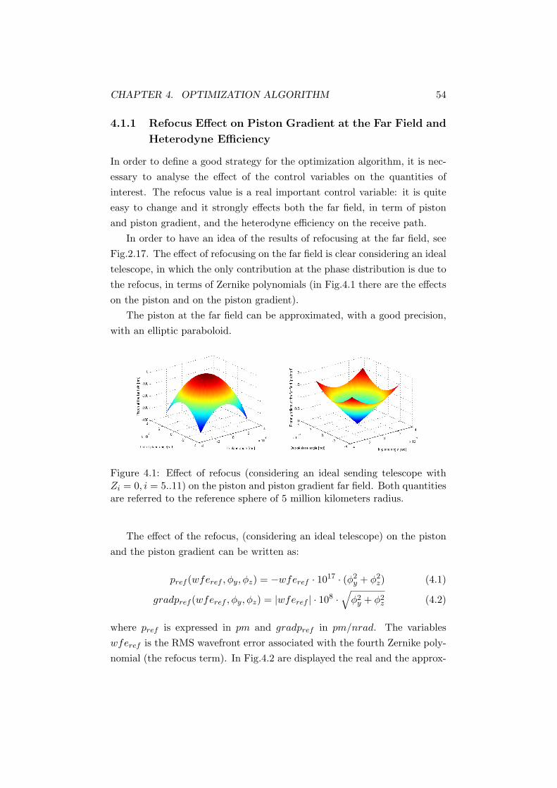
4.1 Approximations Considered . . . . . . . . . . . . . . . . . . . 534.1.1 Refocus Effect on Piston Gradient at the Far Field
and Heterodyne Efficiency . . . . . . . . . . . . . . . . 544.1.2 Pointing Angles Effect on Piston Gradient at the Far
Field and the Heterodyne Efficiency . . . . . . . . . . 574.2 Strategy . . . . . . . . . . . . . . . . . . . . . . . . . . . . . . 614.3 Use of the Point Ahead Angle Mechanism . . . . . . . . . . . 66
5 Results 69
5.1 Results for different Zernike Distributions . . . . . . . . . . . 695.1.1 Starting condition: along geometrical direction . . . . 695.1.2 Starting condition: along null direction in the sense of
DWS . . . . . . . . . . . . . . . . . . . . . . . . . . . . 815.2 Theoretical study . . . . . . . . . . . . . . . . . . . . . . . . . 81
6 Inverse Problem 99
6.1 Assumptions and Goals . . . . . . . . . . . . . . . . . . . . . 996.2 Results . . . . . . . . . . . . . . . . . . . . . . . . . . . . . . . 101
7 Conclusion and Outlook on future work 110
List of Figures
1.1 LISA constellation. . . . . . . . . . . . . . . . . . . . . . . . . 141.2 Metrology chain . . . . . . . . . . . . . . . . . . . . . . . . . . 151.3 Disposition of all the optical elements on the Optical Bench . 161.4 Reference sphere . . . . . . . . . . . . . . . . . . . . . . . . . 171.5 Reference sphere and propagation with ripples . . . . . . . . 18
2.1 Radial functions in Zernike polynomials. . . . . . . . . . . . . 212.2 Contribution of each Zernike term. . . . . . . . . . . . . . . . 232.3 Values of the index a, b in each quadrant of the photodiode . 272.4 Metrology chian, with wavefront. . . . . . . . . . . . . . . . . 292.5 Reference frame and spheres . . . . . . . . . . . . . . . . . . . 302.6 Transmit path on the Optical Bench. . . . . . . . . . . . . . . 312.7 Transmitter beam: field distribution. . . . . . . . . . . . . . . 322.8 Phase field distribution for each Zernike component at the
exit pupil. . . . . . . . . . . . . . . . . . . . . . . . . . . . . . 332.9 Far field: intensity and phase distributions. . . . . . . . . . . 352.10 Phase field distribution for each Zernike component at the far
field. . . . . . . . . . . . . . . . . . . . . . . . . . . . . . . . . 362.11 Piston gradient field distribution for each Zernike component
at the far field. . . . . . . . . . . . . . . . . . . . . . . . . . . 372.12 Piston gradient field distribution for each Zernike component
at the far field. . . . . . . . . . . . . . . . . . . . . . . . . . . 382.13 Receive path on the Optical Bench. . . . . . . . . . . . . . . . 392.14 Receive path on the Quadrant Photodiode. . . . . . . . . . . 392.15 Simplified transmit and receive paths on the Optical Bench,
as considered in the model. . . . . . . . . . . . . . . . . . . . 402.16 Effect of re-pointing the telescope on the far field wavefront. . 41
7
LIST OF FIGURES 8
2.17 Effects of refocusing on the wavefront at the far field. . . . . . 422.18 Effects of PAAM on the wavefront at the far field. . . . . . . 432.19 Misalignment errors included in the model . . . . . . . . . . . 44
3.1 Starting configuration: telescopes facing each other . . . . . . 483.2 Starting configuration: telescopes directed along the null di-
rection . . . . . . . . . . . . . . . . . . . . . . . . . . . . . . . 493.3 Results of each step of ideal optimization with standard Mat-
lab functions . . . . . . . . . . . . . . . . . . . . . . . . . . . 52
4.1 Effect of refocus on the piston and the piston gradient far field 544.2 Piston and piston gradient: real and approximated plot with
the effect of the only refocus, in the operating point . . . . . 554.3 Example of approximation of piston gradient in the operating
point, depending on refocus wavefront error contribute . . . . 564.4 Heterodyne efficiency on quadrant photodiode as function of
refucus weight value . . . . . . . . . . . . . . . . . . . . . . . 574.5 Approximated heterodyne efficiency on quadrant photodiode
as function of refocus weight value . . . . . . . . . . . . . . . 584.6 Piston gradient at the far field: real and approximated fields 594.7 Line Search Method: two cases . . . . . . . . . . . . . . . . . 604.8 Piston gradient at the far field, real and approximated, with
the function evaluations points and results. First case . . . . 614.9 Piston gradient at the far field, real and approximated, with
the function evaluations points and results. Second case . . . 624.10 Heterodyne efficiency depending on the in-plane angle . . . . 634.11 Heterodyne efficiency after the first step of the optimization
algorithm . . . . . . . . . . . . . . . . . . . . . . . . . . . . . 644.12 Piston gradient at the far field, before and after the first step
of the optimization algorithm . . . . . . . . . . . . . . . . . . 654.13 Piston gradient at the far field, before and after the first step
of the optimization algorithm . . . . . . . . . . . . . . . . . . 654.14 Effect of the PAAM on the algorithm results . . . . . . . . . 674.15 Example of approximation of piston gradient at the operating
point, depending on the PAAM out-of-plane angle . . . . . . 68
LIST OF FIGURES 9
5.1 Results: starting condition along geometrical line, wavefronterror Z5 − Z11 = λ/10rms . . . . . . . . . . . . . . . . . . . . 70
5.2 Results: starting condition along geometrical line, wavefronterror Z5 − Z11 = λ/15rms . . . . . . . . . . . . . . . . . . . . 71
5.3 Results: starting condition along geometrical line, wavefronterror Z5 − Z11 = λ/17rms . . . . . . . . . . . . . . . . . . . . 72
5.4 Results: starting condition along geometrical line, wavefronterror Z5 − Z11 = λ/20rms . . . . . . . . . . . . . . . . . . . . 73
5.5 Results: starting condition along geometrical line, wavefronterror Z5 − Z11 = λ/22rms . . . . . . . . . . . . . . . . . . . . 74
5.6 Results: starting condition along geometrical line, wavefronterror Z5 − Z11 = λ/25rms . . . . . . . . . . . . . . . . . . . . 75
5.7 Results: starting condition along geometrical line, wavefronterror Z5 − Z11 = λ/27rms . . . . . . . . . . . . . . . . . . . . 76
5.8 Results: starting condition along geometrical line, wavefronterror Z5 − Z11 = λ/30rms . . . . . . . . . . . . . . . . . . . . 77
5.9 Frequency of heterodyne efficiency values (all quadrants con-sidered) for all the Zernike distributions tested. Initial condi-tion: telescopes directed along the geometrical line connectingthe two test masses . . . . . . . . . . . . . . . . . . . . . . . . 78
5.10 Frequency of piston gradient values for all the Zernike dis-tributions tested. Initial condition: telescopes directed alongthe geometrical line connecting the two test masses. . . . . . 79
5.11 Results: starting condition along null direction, wavefronterror Z5 − Z11 = λ/10rms . . . . . . . . . . . . . . . . . . . . 82
5.12 Results: starting condition along null direction, wavefronterror Z5 − Z11 = λ/15rms . . . . . . . . . . . . . . . . . . . . 83
5.13 Results: starting condition along null direction, wavefronterror Z5 − Z11 = λ/17rms . . . . . . . . . . . . . . . . . . . . 84
5.14 Results: starting condition along null direction, wavefronterror Z5 − Z11 = λ/20rms . . . . . . . . . . . . . . . . . . . . 85
5.15 Results: starting condition along null direction, wavefronterror Z5 − Z11 = λ/22rms . . . . . . . . . . . . . . . . . . . . 86
5.16 Results: starting condition along null direction, wavefronterror Z5 − Z11 = λ/25rms . . . . . . . . . . . . . . . . . . . . 87

LIST OF FIGURES 10
5.17 Results: starting condition along null direction, wavefronterror Z5 − Z11 = λ/27rms . . . . . . . . . . . . . . . . . . . . 88
5.18 Results: starting condition along null direction, wavefronterror Z5 − Z11 = λ/30rms . . . . . . . . . . . . . . . . . . . . 89
5.19 Frequency of heterodyne efficiency values (all quadrants con-sidered) for all the Zernike distributions tested. Initial con-dition: telescopes directed along the null direction. . . . . . . 90
5.20 Frequency of piston gradient values for all the Zernike dis-tributions tested. Initial condition: telescopes directed alongthe null direction. . . . . . . . . . . . . . . . . . . . . . . . . . 91
5.21 Results: final piston gradient in 1000 cases depending on het-erodyne efficiency . . . . . . . . . . . . . . . . . . . . . . . . . 94
5.22 Results: final piston gradient in 1000 cases depending on con-trol variables . . . . . . . . . . . . . . . . . . . . . . . . . . . 95
5.23 Results: final heterodyne efficiency of one quadrant in 1000cases depending on control variables . . . . . . . . . . . . . . 96
5.24 Function evaluations needed in the algorithm, starting withtwo telescopes facing along the geometrical line connectingthe respective test masses . . . . . . . . . . . . . . . . . . . . 97
5.25 Function evaluations needed in the algorithm, starting withtwo telescopes facing along the null direction in the sense ofDWS . . . . . . . . . . . . . . . . . . . . . . . . . . . . . . . . 98
6.1 Effect of each Zernike polynomial on the telescope exit pupil 1036.2 Effect of each Zernike polynomial on the far field piston . . . 1046.3 Effect of each Zernike polynomial on the far field piston gradient1056.4 Error between real and approximated far field piston gradient,
for different Zernike distributions. Evaluation of all termsfrom Z5 to Z11. Blue points correspond to the largest errorfound. . . . . . . . . . . . . . . . . . . . . . . . . . . . . . . . 106
6.5 Real (left) and approximated (right) piston gradient for σ =0.4203. Wavefront error at the pupil λ/10rms. Approxima-tion of all Zernike terms. . . . . . . . . . . . . . . . . . . . . . 107
6.6 Real (left) and approximated (right) piston gradient for σ =0.0567. Wavefront error at the pupil λ/10rms. Approxima-tion of all Zernike terms. . . . . . . . . . . . . . . . . . . . . . 107

LIST OF FIGURES 11
6.7 Error between real and approximated far field piston gradient,for different Zernike distributions. Evaluation of terms Z5-Z6-Z7-Z8 and Z11. Blue points correspond to the largest errorfound. . . . . . . . . . . . . . . . . . . . . . . . . . . . . . . . 108
6.8 Real (left) and approximated (right) piston gradient for σ =1.7562. Wavefront error at the pupil λ/10rms. Approxima-tion of Zernike terms:Z5-Z6-Z7-Z8-Z11. . . . . . . . . . . . . . 109
6.9 Real (left) and approximated (right) piston gradient for σ =1.5172. Wavefront error at the pupil λ/10rms.Approximationof Zernike terms:Z5-Z6-Z7-Z8-Z11. . . . . . . . . . . . . . . . 109
6.10 Real (left) and approximated (right) piston gradient for σ =0.7122. Wavefront error at the pupil λ/15rms.Approximationof Zernike terms:Z5-Z6-Z7-Z8-Z11. . . . . . . . . . . . . . . . 109

List of Tables
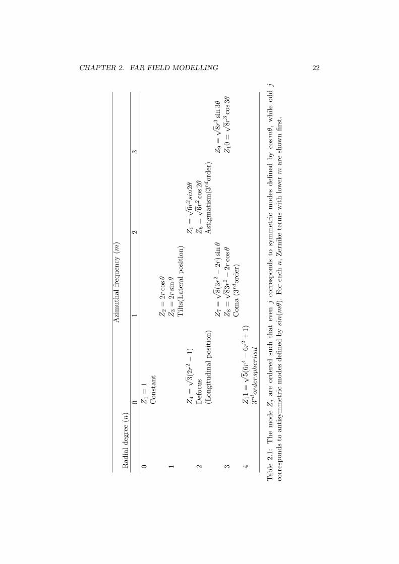
2.1 Zernike polynomials . . . . . . . . . . . . . . . . . . . . . . . 22
3.1 Advantages and disadvantages of different strategies for theideal optimization. . . . . . . . . . . . . . . . . . . . . . . . . 50
5.1 Mean value µ and standard deviation σ of heterodyne ef-ficiency and piston gradient resulted when as starting con-dition the telescopes are directed along the geometrical lineconnecting the two test masses. . . . . . . . . . . . . . . . . . 80
5.2 Mean value µ and standard deviation σ of heterodyne effi-ciency and piston gradient resulted when as starting conditionthe telescopes are directed along their null direction. . . . . . 92
12
Chapter 1
Introduction
1.1 LISA Mission Overview
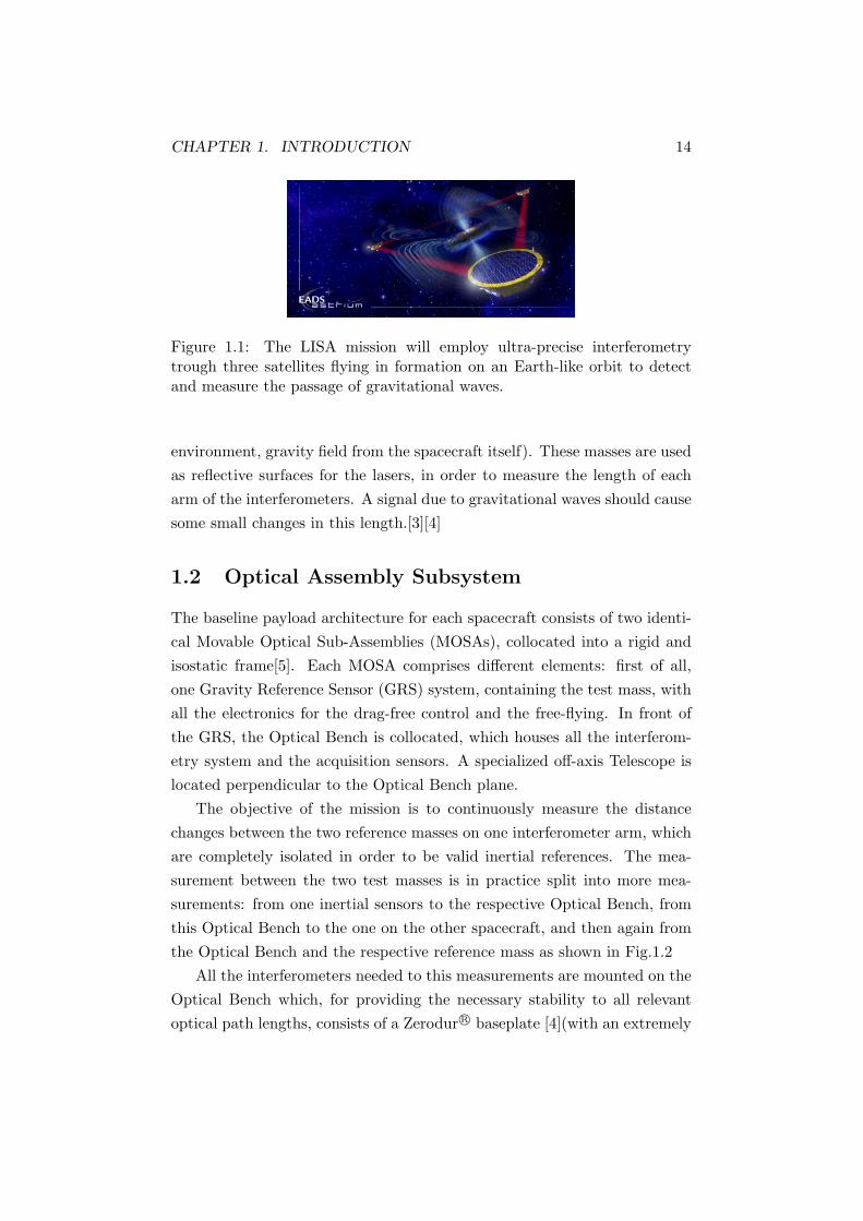
The Laser Interferometer Space Antenna (LISA) is a cooperative missionbetween ESA and NASA, aimed to detect and observe gravitational waves,predicted by the Theory of General Relativity [1][2]. Gravitational wavesshould be generated by great astrophysical objects or events, like super-massive black holes and ultra-compact galactic binaries.
The main goal the LISA Mission is the detection of low frequency gravi-tational radiation, in a measurement band width between 0.1mHz and 1Hz,a range exactly complementary to a number of ground-based interferometers(LIGO, VIRGO, TAMA 300 and GEO 600), which cannot reach this lowfrequency range because of their intrinsic sensitivity due to the Earth’s owngravitational field and seismic activity.
The mission uses laser interferometry, implemented in a constellation ofthree spacecraft, which are arranged in a quasi-equilateral triangle form,with an arm-length of 5 millions kilometers, in a heliocentric orbit witha semi-major axis of 1 AU. Each spacecraft carries a V-shaped payload,composed of two test masses, with their laser measurements and associatedelectronics. Two arms of this triangle form a Michelson interferometer.
The inertial references for the mission consist of the two ”proof masses”on each spacecraft which act as the end mirror of a single-arm interfer-ometer. These targets are free-flying and drag-free controlled, in order toavoid displacements due to external forces that are not due to gravity (e.s.spacecraft maneuvers, solar radiation pressure, magnetic fields, outgassing
13
CHAPTER 1. INTRODUCTION 14
Figure 1.1: The LISA mission will employ ultra-precise interferometrytrough three satellites flying in formation on an Earth-like orbit to detectand measure the passage of gravitational waves.
environment, gravity field from the spacecraft itself). These masses are usedas reflective surfaces for the lasers, in order to measure the length of eacharm of the interferometers. A signal due to gravitational waves should causesome small changes in this length.[3][4]
1.2 Optical Assembly Subsystem
The baseline payload architecture for each spacecraft consists of two identi-cal Movable Optical Sub-Assemblies (MOSAs), collocated into a rigid andisostatic frame[5]. Each MOSA comprises different elements: first of all,one Gravity Reference Sensor (GRS) system, containing the test mass, withall the electronics for the drag-free control and the free-flying. In front ofthe GRS, the Optical Bench is collocated, which houses all the interferom-etry system and the acquisition sensors. A specialized off-axis Telescope islocated perpendicular to the Optical Bench plane.
The objective of the mission is to continuously measure the distancechanges between the two reference masses on one interferometer arm, whichare completely isolated in order to be valid inertial references. The mea-surement between the two test masses is in practice split into more mea-surements: from one inertial sensors to the respective Optical Bench, fromthis Optical Bench to the one on the other spacecraft, and then again fromthe Optical Bench and the respective reference mass as shown in Fig.1.2
All the interferometers needed to this measurements are mounted on theOptical Bench which, for providing the necessary stability to all relevantoptical path lengths, consists of a Zerodur R© baseplate [4](with an extremely

CHAPTER 1. INTRODUCTION 15
Figure 1.2: Metrology chain. The measurements are computed between theInertial Sensor 1 (IS1) and the Optical Bench 1, from the Optical Bench1(OB1) and the Optical Bench 2 (OB2), from the Optical Bench 2 and theInertial Sensor 2 (IS2).
low cTE of 2 ∗ 10−8K−1). A picture of the disposition of all the opticalelements is sketched in Fig.1.3.
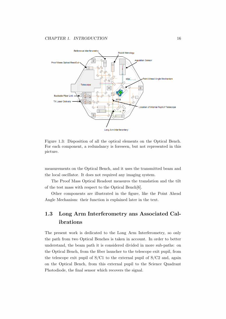
As can be seen in Fig.1.3, in each Optical Bench three laser frequenciesare used. In addition to the received and the transmitted beam (which gofor 5 millions kilometers to and from the other spacecraft), there is one otherlaser, called Local Oscillator, which is furnished by the Backside Fiber Link.This same laser is used as the transmitted beam for the other MOSA onthe same spacecraft. When used as local oscillator, it become the referencelaser for all the measurements on the respective Optical Bench.
Each Optical Assembly contains three main interferometers: the LongArm Interferometer (Science Interferometer), the Reference Interferometer,and the Proof Mass Optical Readout. For each of these, a redundancy ispresent.
The Science Interferometer uses the received beam and the local oscil-lator, but the detection of the phase of the received beam is limited by theshot-noise (the RX beam has a power of around 100pW ). For decouplingtranslation and tilt metrology, it is mandatory for the Long Arm Interferom-eter to have an imaging system. In this case, it is a Differential WavefrontSensing. It gives information about the wavefront tilt of the received beam,and also about the local aberrations of the telescope and the power received.In practice, it is used to define the pointing of one telescope with respect tothe incoming wavefront, in tip and tilt.
The Reference Interferometer establishes a phase reference for all the
CHAPTER 1. INTRODUCTION 16
Figure 1.3: Disposition of all the optical elements on the Optical Bench.For each component, a redundancy is foreseen, but not represented in thispicture.
measurements on the Optical Bench, and it uses the transmitted beam andthe local oscillator. It does not required any imaging system.
The Proof Mass Optical Readout measures the translation and the tiltof the test mass with respect to the Optical Bench[6].
Other components are illustrated in the figure, like the Point AheadAngle Mechanism: their function is explained later in the text.
1.3 Long Arm Interferometry ans Associated Cal-
ibrations
The present work is dedicated to the Long Arm Interferometry, so onlythe path from two Optical Benches is taken in account. In order to betterunderstand, the beam path it is considered divided in more sub-paths: onthe Optical Bench, from the fiber launcher to the telescope exit pupil, fromthe telescope exit pupil of S/C1 to the external pupil of S/C2 and, againon the Optical Bench, from this external pupil to the Science QuadrantPhotodiode, the final sensor which recovers the signal.

CHAPTER 1. INTRODUCTION 17
In order to understand the aim of this work, a more detailed descriptionof the far field propagation (from the exit pupil of S/C1 to external pupil ofS/C2) is mandatory.
In this project, a beam with a Gaussian intensity profile is sent for 5million kilometers, starting from an exit pupil with a radius of 20 cm. Itpropagates in free space, and, at 5 million kilometers of distance, the wave-front profile is very similar to a perfect sphere. The center of this sphere isthe phase center of the beam. By knowing the curvature of the sphere insome points of the far field, it is possible to compute the phase center offset,with respect to a defined reference system (Fig.1.4).
Figure 1.4: Results of geometrical phase center offset for an ideal beampropagating in free space.
But it should be consider that the transmitted beam has passed throughan optical system (the telescope, but also all the mirrors and mechanismson the Optical Bench), so as explained in Par.2.1.1, its phase has beenmodified. At 5 million kilometers of distance, its wavefront is not a perfectsphere, but there are ripples on it due to the optical aberrations introducedby passing through the optical systems. This effect introduces an error inthe evaluation of the real phase center offset (optical phase center offset), asshown in Fig.1.5.
For having useful information about these effects, a reference sphere isdefined with a radius of 5 million kilometers, centered in the respective testmass. The wavefront phase piston and phase slope are defined and computedwith respect to this sphere. We call phase piston the distance in pm from

CHAPTER 1. INTRODUCTION 18
Figure 1.5: Propagation in free space of a beam containing optical aberra-tions. There are some ”‘ripples”’ on it of some pm. From the measure of thelocal wavefront curvature, it can be found the optical phase center offset.
the reference sphere to the real wavefront; its slope, with respect to thereference sphere in the two angular directions, is the phase slope(usuallymeasured in pm/nrad).
The phase slope in the far field, as previously defined, is a measure ofthe phase center offset, with a ”noise” introduced by the optical aberrations,which changes the far field wavefront.
Similar problems are present in the received path. The beam enters thetelescope and arrives on the Science Quadrant Photodiode, but it has passedthrough an optical system, so its phase has changed because of the intro-duction of the optical aberrations. Due to this effect, the direction of thereceiver wavefront is not exactly the same of the telescope axis. Thanks tothe imaging system (Differential Wavefront Sensing), it is possible to changethe orientation of the receiver telescope, in order to have a wavefront per-fectly perpendicular on the photodiode (a wavefront tilt on the photodiode,as in the transmitted path, corresponds in fact to a phase center offset).
For having an idea of these effects at the far field, it has been estimatedthat the geometrical and the optical phase center offsets yield a piston effectat the far field of several pm. As this point, it is necessary to consider thatthe direction of the telescope is not strictly fixed, but it jitters with severalnrad/
√Hz. This effect, in practice, changes continuously the phase piston
at the operational point if the phase slope is too high.

CHAPTER 1. INTRODUCTION 19
The knowledge of the phase center offset (for both transmit and receivedbeams) is then really useful for the success of the mission, because it sig-nificantly decreases the measurement performance, being coupled with theangular motion of the telescope. An appropriate calibration is then manda-tory, to compensate these effects [7]. In order to do this, a test signal (sinesignal) is used, injected in the telescope pointing and the piston effect ismeasured. These results are used to adjust telescope refocus and pointingas well as in data processing on ground.

Chapter 2
Far Field Modelling
2.1 Modelling Aspects and Assumptions
This section is dedicated to clarify some more theoretical aspects of theproject, studied and considered during the modelling. One of these, thepart dedicated to the Zernike field, is really important, because on thissubject all the statistical studies presented later are based.
2.1.1 Zernike Field
The Zernike polynomials are a well known mathematical formulation todescribe the classical aberrations of an optical system. In this work, thenormalization found by Noll is used [8].
The Zernike polynomials are a set of polynomials defined on a unit cir-cle. Using polar coordinates, they can be written like a product of an angu-lar function and radial polynomials. The modified polynomials of Noll areslightly different from the standard ones, but they are particularly useful forstatistical analysis. The polynomials are defined as:
Zevenj =√
n + 1Rmn (r)√
2 cos mθ
Zoddj=√
n + 1Rmn (r)√
2 sinmθ
}m 6= 0 (2.1)
Zj =√
n + 1R0n(r) m = 0 (2.2)
where
Rmn (r) =
(n−m)/2∑s=0
(−1)s(n− s)!
s![
(n+m)2 − s
]![
(n−m)2 − s
]!)
rn−2s (2.3)
20
CHAPTER 2. FAR FIELD MODELLING 21
The value of n and m are always integral and satisfy:
m ≤ n
n− |m| = even
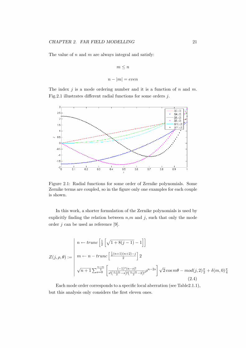
The index j is a mode ordering number and it is a function of n and m.Fig.2.1 illustrates different radial functions for some orders j.
Figure 2.1: Radial functions for some order of Zernike polynomials. SomeZernike terms are coupled, so in the figure only one examples for each coupleis shown.
In this work, a shorter formulation of the Zernike polynomials is used byexplicitly finding the relation between n,m and j, such that only the modeorder j can be used as reference [9].
Z(j, ρ, θ) :=
∣∣∣∣∣∣∣∣∣∣∣∣∣∣
n← trunc[
12
[√1 + 8(j − 1)− 1
]]m← n− trunc
[ 12(n+1)(n+2)−j
2
]2
√n + 1
∑n−m2
s=0
[(−1)s(n−s)!
s!(n+m2
−s)!(n−m2
−2)!ρn−2s
]√2 cos mθ −mod(j, 2)π
2 + δ(m, 0)π4
(2.4)Each mode order corresponds to a specific local aberration (see Table2.1.1),
but this analysis only considers the first eleven ones.
CHAPTER 2. FAR FIELD MODELLING 22
Azi
mut
halfr
eque
ncy
(m)
Rad
ialde
gree
(n)
01
23
0Z
1=
1C
onst
ant
Z2
=2r
cosθ
1Z
3=
2rsi
nθ
Tilt
s(Lat
eral
posi
tion
)Z
4=√
3(2r
2−
1)Z
5=√
6r2si
n2θ
2D
efoc
usZ
6=√
6r2co
s2θ
(Lon
gitu
dina
lpo
siti
on)
Ast
igm
atis
m(3
rdor
der)
Z7
=√
8(3r
2−
2r)s
inθ
Z9
=√
8r3si
n3θ
3Z
8=√
83r2−
2rco
sθZ
10
=√
8r3co
s3θ
Com
a(3
rdor
der)
4Z
11
=√
5(6r
4−
6r2+
1)3r
dor
der
spher
ical
Tab
le2.
1:T
hem
ode
Zj
are
orde
red
such
that
even
jco
rres
pond
sto
sym
met
ric
mod
esde
fined
byco
smθ,
whi
leod
dj
corr
espo
nds
toan
tisy
mm
etri
cm
odes
defin
edby
sin(m
θ).
For
each
n,Zer
nike
term
sw
ith
low
erm
are
show
nfir
st.

CHAPTER 2. FAR FIELD MODELLING 23
In order to better understand the effects of each order contribution,Fig.2.2 shows the aberrations introduced by each component on the unitcircle (from the fourth to the eleventh) in terms of phase distribution, usingas a starting beam a plane wave with phase zero.
Figure 2.2: Plots of the value of the phase distribution on an unit circle.These aberrations are applied on a plane wave with phase zero.
In the following analysis, all the terms from 2 to 11 are considered: theterm Z1, according to Noll, is disregarded, because it gives a constant offsetto the complete field on the unit circle. The terms Z2 and Z3, identified asconsequence of tilt in the two directions, are explicitly taken into account inthe following model, so for the moment, they are neglected. At this point,a vector of weights wfe is defined, for defining the specific contributions ofthe individual Zernikes in terms of an rms wavefront error. As explainedabove, only the coefficients from startZ = 4 to endZ = 11 of this vector areevaluated in the model.
Each beam passing through an optical system changes its phase distri-bution, due to these Zernike terms. In the model this effect is expressedas:

CHAPTER 2. FAR FIELD MODELLING 24
ΦZ(x, z) :=
∣∣∣∣∣∣∣∣∣∣∣∣
ρ←√
x2+y2
r0
θ ← arctan( yx+1−sign(ρ))
2 · π ·∑endZ
j=startZ(wfej · Z(j, ρ, θ))
(2.5)
where the definition of θ has been slightly modified in order to avoid thecase arctan(y
0 ) and the value of ΦZ is depending, as explained before, onlyon the Zernike terms from 4 to 11.
2.1.2 Propagation of Light in Free Space
This paragraph is an introduction to Fourier Optics, which describes thepropagation of light waves based on harmonic analysis, first of all Fouriertransformations [10]. This represents the theoretical basis on which thewhole model of the Long Arm Interferometry is built upon.
It is considered an arbitrary function f(x, y) of two variables x and y,which are the spatial coordinates. The same function can be written as asuperposition of harmonic functions of x and y in the form:
f(x, y) = F (νx, νy) exp [−j2π(νxx + νyy)] (2.6)
where F (νx, νy) is the complex amplitude and νx and νy are the spatialfrequencies.
Now, a plane wave is defined in this form:
U(x, y, z) = A exp [−j(kxx + kyy + kzz)] (2.7)
where kx, ky and kz are the components of the wave vector k and A isa complex constant. In the plane z = 0, the plane wave U(x, y, z) is thearbitrary function f(x, y) = A exp [−j2π(νxxνyy)], where νx = kx/2π andνy = ky/2π are the spatial frequencies (cycles/mm), while kx and ky arethe spatial angular frequencies (radians/mm).
From the Fourier analysis, it is known that there is a one-to-one corre-spondence between plane wave and spatial harmonic function if the spatialfrequency does not exceed the inverse of the wavelength (1/λ), and, more in

CHAPTER 2. FAR FIELD MODELLING 25
details, it is known that:
f(x, y) = U(x, y, 0) (2.8)
U(x, y, z) = f(x, y) exp (−jkzz) (2.9)
where, in the last one, kz = ±(k2− k2x− k2
y)12 and k = 2π/λ. A condition of
validity is that k2x + k2
y < k2, so kz is real.If a plane wave of unity amplitude is transmitted through an optical sys-
tem with complex amplitude transmittance f(x, y), the wave is modulatedby the harmonic function such that U(x, y, 0) = f(x, y). In a general case,if f(x, y) is a superposition integral of harmonic functions:
f(x, y, ) =∫ ∞
−∞
∫ ∞
−∞F (νx, νy) exp [−j2π(νxx + νyy)] dνx dνy (2.10)
with frequencies νx, νy and amplitudes F (νx, νy), the transmitted wave is:
U(x, y, z) =∫ ∞
−∞
∫ ∞
−∞F (νx, νy) exp [−j(2πνxx + 2πνyy)] exp (−jkzz) dνx dνy
(2.11)with complex envelopes F (νx, νy) and where kz = (k2−k2
x−k2y)
12 = 2π( 1
λ2 −ν2
x − ν2y)
12 .
A brief analysis on the propagation of monochromatic optical wave ispresented, starting from this basis. A wave with wavelength λ and complexamplitude U(x, y, z) is propagating in free space between the planes z = 0and z = d. The complex amplitude at the input plane is f(x, y) = U(x, y, 0)and at the output plane g(x, y) = U(x, y, d).
The functions f(x, y) and g(x, y) can also be considered as input andoutput of a linear and shift-invariant system (due to the invariance of freespace to displacement of a coordinate system). In order to characterize thesystem, it is necessary to define its transfer function H(νx, νy), or its impulseresponse h(x, y).
Considering that f(x, y) = A exp [−j2π(νxx + νyy)] = A exp [−j(kxx + kyy)]and g(x, y) = A exp [−j(kxx + kyy + kzd)], it is possible to write H(νx, νy)as g(x,y)
f(x,y) :
H(νx, νy) = exp[−j2π(
1λ2− ν2
x − ν2y)
12 d
](2.12)
If the input function f(x, y) contains only spatial frequencies that are much
CHAPTER 2. FAR FIELD MODELLING 26
smaller than the cutoff frequency 1/λ (ν2x+ν2
y << 1/λ2), then the expressionof the transfer function can be significantly simplified:
H(νx, νy) ≈ H0 exp[jπλd(ν2
x + ν2y)]
(2.13)
where H0 = exp (−jkd). In this form, the transfer function of free space isknown as the Fresnel approximation.
Then, having a certain input function f(x, y), at this point its Fouriertransformation can be defined as:
F (νx, νy) =∫ ∞
−∞
∫ ∞
−∞f(x, y) exp [j2π(νxx + νyy)] dx dy (2.14)
which is the envelope of plane wave components in the input plane. Thesame quantity, computed on the output plane is obtained from H(νx, νy) ·F (νx, νy). From this one, using the inverse transformation:
g(x, y) =∫ ∞
−∞
∫ ∞
−∞H(νx, νy)F (νx, νy) exp [−j2π(νxx + νyy)] dνx dνy
(2.15)The impulse response is the inverse transformation of H(νx, νy) and with
the Fresnel approximation can be written as:
h(x, y) ≈ h0 exp[−jk
x2 + y2
2d
](2.16)
where h0 = (j/kd) exp (−jkd).An alternative way to proceed is to define the function g(x, y) as a con-
volution between f(x, y) and the impulse response:
g(x, y) = h0
∫ ∞
−∞
∫ ∞
−∞f(x′, y′) exp
[−jπ
(x− x′)2 + (y − y′)2
λd
]dx′ dy′
(2.17)where h0 is the previous one.
2.1.3 Heterodyne Efficiency
The heterodyne efficiency is a measure of the quality of the signal on theimaging sensor. In this case, it is represented from the Quadrant Photodi-ode, so for each MOSA four efficiencies are computed, one for each quadrantof the sensor. For the moment, it is possible to explain the meaning of this

CHAPTER 2. FAR FIELD MODELLING 27
measure using general signals; later in the thesis a more specific definitionof the same fields is given.
In order to compute the efficiency, two signals are necessary: a receivedone and a reference one. The received signal is the received field from thedeep space, ERX , while the reference signal is the field furnished by the localoscillator ELO. :
ε(Φy,Φz, a, b) :=
(∣∣∣∣∫ a·r0
0
∫ b·√
r20−y2
0 ERX(y, z,Φy,Φz) · ELO(y, z) dz dy
∣∣∣∣)∫ a·r0
0
∫ b·√
r20−y2
0 (|ERX(y, z,Φy,Φz)|)2 dz dy
·
(∣∣∣∣∫ a·r0
0
∫ b·√
r20−y2
0 ERX(y, z,Φy,Φz) · ELO(y, z) dz dy
∣∣∣∣)∫ a·r0
0
∫ b·√
r20−z2
0 (|ELO(y, z)|)2 dz dy
(2.18)
In this case, ERX is a generic field coming from the space, dependingon two spatial coordinates (perpendicular to the telescope axis) and on theangular tilts in the two direction. The local oscillator field ELO is a generalelectric field depending only on the spatial coordinates.
In equation 2.18, the terms a and b can assume only the values ±1 andthey represent an index for the quadrant considered (Fig.2.3).
Figure 2.3: Values of the index a, b in each quadrant of the photodiode.
The value of the efficiency computed in this way is a sort of measure-ment of the power received in the quadrant area compared with the powertransmitted by the two signals used.
The only way to change the heterodyne efficiency of a quadrant photo-diode is to change the tilt of the incoming wavefront with respect to the

CHAPTER 2. FAR FIELD MODELLING 28
orientation of the sensor. Another way is to reduce the optical aberrationsintroduced, which at the end modify the received beam along its paths fromthe external pupil of the telescope to the photodiode sensor.
In the starting formulation, the heterodyne efficiency was computed us-ing the dblquad function of Matlab, but in this case the integral computationresulted too slow. In the final version it has been substituted with a fasterapproach: the integral is evaluated on a fix grid that covers the all area ofthe quadrant photodiode [11].
2.2 One Arm-Interferometry Model
2.2.1 Metrology Chain
The model implemented in this project takes into account the measurementsbetween two Optical Benches and it is representative for only one arm of theinterferometry. Each one of the two spacecraft considered in this analysis,is at the same time transmitter and receiver.
One transmitted laser is injected on the Optical Bench 1 (OB1) and,after some necessary reflections and re-directioning on the optical plate,goes out from the respective telescope (T1). After 5 million kilometers,it enters telescope T2. Here, it is interfered with the local oscillator, anddetected on the quadrant photodiode. From the signal of the DifferentialWavefront Sensing, spacecraft S/C2 is re-pointed along a better direction.This scheme is absolutely symmetric, so it is valid in both directions. Fig.2.4depicts the metrology chain and at each step there is a picture of a testingphase obtained with the implemented model. As shown, the optical systemand the propagation into the far field can significantly modify the originalphase of the transmitted beam.
2.2.2 Reference Coordinate Frames
In the model three reference coordinate frames are used. Two referenceframes are defined by the two telescopes, where the x-direction correspondsto the telescope axis. As an inertial reference, a third fixed frame is presentin the model.
As previously mentioned, all the measurements are taken with respectto an ideal sphere of 5 million kilometers radius. The center of this reference

CHAPTER 2. FAR FIELD MODELLING 29
Figure 2.4: The metrology chain used to implemented a model for one armof the interferometry. In this picture, only the beam path in one directionis shown, with the wavefront computed with the model at each measuringstep.
sphere is, for each spacecraft, the center of the test mass. The wavefront atthe far field is always referred to this sphere in order to avoid computationalerrors due to the giant distance traveled from the beam compared to itssmall wavelength (λ = 1064 · 10−9m).
The two spacecraft are at the fixed distance of 5 million kilometers, thenS/C1 is positioned on the sphere originated from the test mass on spacecraftS/C2 and vice versa. The orientation of the two frames is at the momentcompletely independent (see Fig.2.5).
The orientation of the frame determines the incoming wavefront direc-tion, but,less obvious, this variable is a function also of the position on thesphere because of the ripples of the wavefront since the optical aberrationshave a certain distribution on the reference sphere. Clearly, the positionof one spacecraft on the sphere generated from the other one influencesnot only the direction of the incoming wavefront, but also the amount ofpower received. The position has some constraints on this sense, becausea minimum amount of power received is necessary in order to generate anappreciable signal.

CHAPTER 2. FAR FIELD MODELLING 30
Figure 2.5: The draws represents the reference spheres of the two spacecraft,and explains the concept of phase center offset in one sending direction.The receiver telescope (T2) is in some point on the sphere generates fromthe spacecraft 1 (blue). Due to this position and orientation, it sees theincoming wavefront with a certain tilt, and find the phase center in somepoint at million kilometers of distance. The yellow line is the offset of thecomputed position to the real one.
2.2.3 Transmitted beam and Far Field Propagation Results
The beam used in this model as a transmitter is a Gaussian beam. It is aspecial optical wave, with the power concentrated within a small cylinderaround the beam axis. The intensity distribution in any transverse plane is acircularly symmetric Gaussian function, centered about the beam axis. Thewidth of this function is minimum at the beam waist and grows graduallyin all directions. The wavefronts are almost planar near the beam waistand become approximately spherical far from the waist [10]. Under idealconditions, the light from a laser takes the form of a Gaussian beam, andthis is the reason why it has been used in the model.
The electric field of a classical Gaussian beam is defined (in a reference

CHAPTER 2. FAR FIELD MODELLING 31
frame where the telescope axis is the x-axis and where the frame center isthe pupil center of the telescope)as:
EG(x, y, z, wy, wz, fy, fz, P ) :=
√cost · P
wywz [(1 + jτ(x, fy, wy))(1 + jτ(x, fz, wz))]
exp[jkx− y2
w2y(1 + jτ(x, fy, wy))
− z2
w2z(1 + jτ(x, fz, wz))
](2.19)
τ(z, f, w0) :=z − f
πw20
λ (2.20)
where: wy and wz are the beam waist radius in the two directions, fy andfz are the focal point coordinates with respect to the pupil center of thetelescope and P is the power of the beam [9]. The variable cost is a constantfunction defined as:
cost :=4
cε0π(2.21)
where ε0 is the permittivity of free space and c the speed of the light.The function used as an input (f(x, y) in Par.2.1.2) for the propagation
in the far field, is not really this form of Gaussian beam. Before going out inthe free space, the beam has to passed through some optical elements (seeFig.2.6), which modify the phase distribution.
Figure 2.6: The green line represents the transmitted beam, passing throughsome optical elements on the Optical Bench, an then going out from thetelescope.
For this reason, the input function used in the model is a beam with aGaussian intensity profile and the phase defined with the Zernike polynomi-als, following the concepts explained in Par.2.1.1. It is assumed that all the

CHAPTER 2. FAR FIELD MODELLING 32
terms in Eq.2.19 that can introduce some phase different from zero, are null(τ(x, f, w0) is identically to zero).
Using the reference frame described in Par.2.2.2, the transmitted beam,whichis the input function for the free-space propagation is defined as:
Einput(y, z,∆y, ∆z, wy, wz, P ) =
√costP
wywz
· exp
[−(
y −∆y
wy
)2
−(
z −∆z
wz
)2]· exp (jΦx(y, z))
(2.22)
where Φx(y, z) is the Zernike distribution defined in Par.2.1.1, ∆y and ∆z
represent the lateral offset of the intensity peak from the pupil center. In Fig2.7 there is an example of the intensity and phase profile for the transmittedbeam, with a randomly chosen Zernike distribution. In order to see theeffect of the weight value for the Zernike terms on the phase distributionFig.2.8 illustrates the phase field caused by each Zernike term previouslygenerated on the exit pupil.
Figure 2.7: Example of intensity profile (gaussian distribution) and phaseprofile, for the transmitted beam, when it goes out of the telescope.
Using this particular beam, it is possible to compute the far field prop-agation as described in Par.2.1.2. In the following is reported the Equation2.17 for clearness:
g(x, y) = h0
∫ ∞
−∞
∫ ∞
−∞f(x′, y′) exp
[−jπ
(x− x′)2 + (y − y′)2
λd
]dx′ dy′

CHAPTER 2. FAR FIELD MODELLING 33
Figure 2.8: Contribute of each Zernike term to the final phase distributionon the exit pupil.
where g(x, y) is the resulting field, f(x,y) is the input field, and
h0 = (j/kd) exp (−jkd)
The variable d is the distance from the input plane and the output plane. Inthe present case, the Fresnel approximation is valid (spatial frequencies >>
1/λ) , the function f(x, y) is the input field previously defined Einput(y, z)and g(x, y) is the resulted field on the reference sphere, which is calledEff (y, z, d,∆d). In this form (y, z) are the spatial coordinates perpendicularto the main direction (x-axis corresponds to the telescope axis direction),d is the distance on the x-axis for which the phase-offset is set to zero and∆d is the deviation from this distance. So, in the case of the transmitted
CHAPTER 2. FAR FIELD MODELLING 34
gaussian beam, at the far field the field becomes:
Eff (y, z, d,∆d) :=j
λ(d−∆xS)· exp (−jk∆d) ·
∫ r0
0
∫ 2π
0Einput(r cos φ, r sinφ)·
exp[−jπ · (y − r cos φ−∆yS)2 + (z − r sinφ−∆zS)2
λ · (d−∆xS)
]· r dφ dr
(2.23)
At this point, a coordinate transformation is necessary in order to referthe calculation to the far field reference sphere.
y(φy, φz) := L ·(
1− φ2z
2
)· φy (2.24)
z(φz) := L · φz (2.25)
d(φy, φz) := L ·
(1−
φ2y
2
)·(
1− φ2z
2
)(2.26)
∆d(φy, φz) := −L ·φ2
y + φ2z
2(2.27)
In this way the far field can be written as a function of angular coordinates:
Effsphere= Eff (y(φy, φz), z(φz), d(φy, φz),∆d(φy, φz)) (2.28)
Now it is possible to have a mathematical definition for the piston: it isthe measure of the far field phase in terms of wavelength, expressed in pm.So, it can be written:
pff (φy, φz) := arg (Effsphere(φy, φz)) ·
λ
2π· 1012 (2.29)
and for the phase slope (also called piston gradient, from its derivation),expressed in pm/nrad:
gradpff (φy, φz) := norm
(∂pff (φy, φz)
∂φy,∂pff (φy, φz)
∂φz
)(2.30)
Figure 2.9 represents the same beam reported before after its far fieldpropagation. The figure shows the intensity and phase profile, even if duringthe project the quantity taken into account is the piston, and not the phase.
As done before, Fig.2.10 shows the effect of each Zernike term taken inaccount on the far field phase distribution.

CHAPTER 2. FAR FIELD MODELLING 35
Figure 2.9: Far field: on the left side the intensity field, on the right sidethe phase distribution.
The phase is not a quantity taken into account during the project: theresults of the work in fact refers to the piston (Eq.2.29) and the pistongradient (Eq.2.30), as explained before. They always represent a measure ofthe phase and its slope, but expressed in terms of pm and pm/nrad. For thisreason Fig.2.11 and Fig.2.12 show these two fields near the operating pointat the far field, and the effect of each Zernike term on the piston gradientdistribution.
2.2.4 Received beam
Each telescope receives a small amount of the laser transmitted from an-other telescope. The aperture of the telescope which can absorb the lighttransmitted has a diameter of 40cm. The curvature of the beam transmittedis comparable with the sphere of 5 millions kilometers of radius. Then thewavefront entering the telescope is with a great precision a plane wave.
Also the received beam has to pass through some optical elements(Fig.2.13)before being detected on the quadrant photodiode, so in the model it is as-sumed that the phase of the beam is completely depending on the Zernikepolynomials of the system, defined in Par. 2.1.1.
The equation representing the received field is:
ERX(y, z, tilty, tiltz) :=
√costPRX
2r20
exp[j
[Φ(y, z) +
4π
r0(tiltyy + tiltzz)
]](2.31)
where tilty and tiltz are the inclinations of the beam with respect to thetelescope axis (x-axis in this reference frame),PRX is the received power,
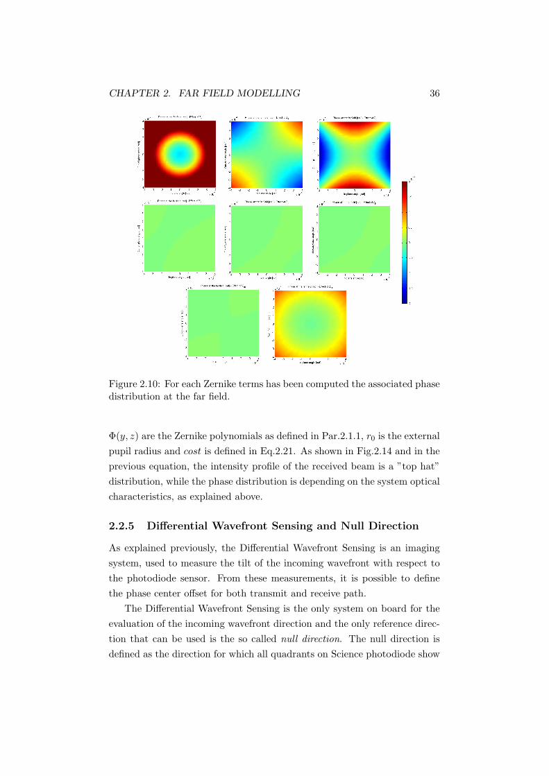
CHAPTER 2. FAR FIELD MODELLING 36
Figure 2.10: For each Zernike terms has been computed the associated phasedistribution at the far field.
Φ(y, z) are the Zernike polynomials as defined in Par.2.1.1, r0 is the externalpupil radius and cost is defined in Eq.2.21. As shown in Fig.2.14 and in theprevious equation, the intensity profile of the received beam is a ”top hat”distribution, while the phase distribution is depending on the system opticalcharacteristics, as explained above.
2.2.5 Differential Wavefront Sensing and Null Direction
As explained previously, the Differential Wavefront Sensing is an imagingsystem, used to measure the tilt of the incoming wavefront with respect tothe photodiode sensor. From these measurements, it is possible to definethe phase center offset for both transmit and receive path.
The Differential Wavefront Sensing is the only system on board for theevaluation of the incoming wavefront direction and the only reference direc-tion that can be used is the so called null direction. The null direction isdefined as the direction for which all quadrants on Science photodiode show
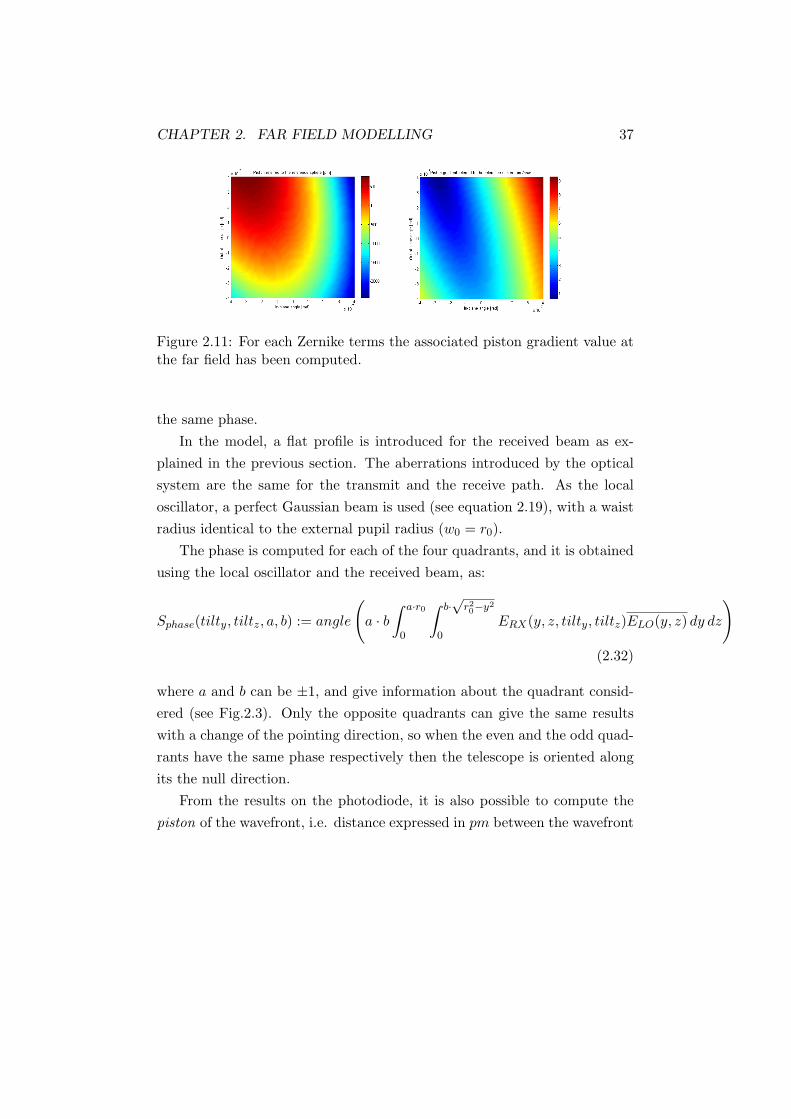
CHAPTER 2. FAR FIELD MODELLING 37
Figure 2.11: For each Zernike terms the associated piston gradient value atthe far field has been computed.
the same phase.In the model, a flat profile is introduced for the received beam as ex-
plained in the previous section. The aberrations introduced by the opticalsystem are the same for the transmit and the receive path. As the localoscillator, a perfect Gaussian beam is used (see equation 2.19), with a waistradius identical to the external pupil radius (w0 = r0).
The phase is computed for each of the four quadrants, and it is obtainedusing the local oscillator and the received beam, as:
Sphase(tilty, tiltz, a, b) := angle
(a · b
∫ a·r0
0
∫ b·√
r20−y2
0ERX(y, z, tilty, tiltz)ELO(y, z) dy dz
)(2.32)
where a and b can be ±1, and give information about the quadrant consid-ered (see Fig.2.3). Only the opposite quadrants can give the same resultswith a change of the pointing direction, so when the even and the odd quad-rants have the same phase respectively then the telescope is oriented alongits the null direction.
From the results on the photodiode, it is also possible to compute thepiston of the wavefront, i.e. distance expressed in pm between the wavefront
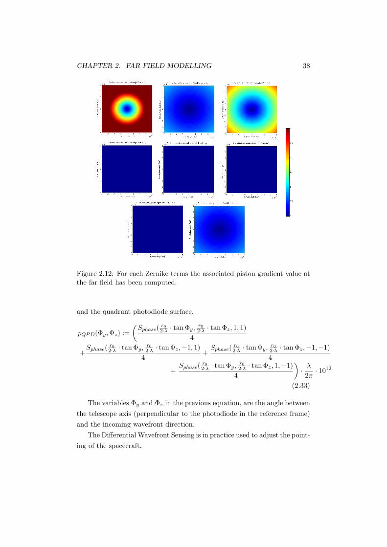
CHAPTER 2. FAR FIELD MODELLING 38
Figure 2.12: For each Zernike terms the associated piston gradient value atthe far field has been computed.
and the quadrant photodiode surface.
pQPD(Φy,Φz) :=(
Sphase( r02·λ · tanΦy,
r02·λ · tanΦz, 1, 1)
4
+Sphase( r0
2·λ · tanΦy,r02·λ · tanΦz,−1, 1)
4+
Sphase( r02·λ · tanΦy,
r02·λ · tanΦz,−1,−1)4
+Sphase( r0
2·λ · tanΦy,r02·λ · tanΦz, 1,−1)
4
)· λ
2π· 1012
(2.33)
The variables Φy and Φz in the previous equation, are the angle betweenthe telescope axis (perpendicular to the photodiode in the reference frame)and the incoming wavefront direction.
The Differential Wavefront Sensing is in practice used to adjust the point-ing of the spacecraft.
CHAPTER 2. FAR FIELD MODELLING 39
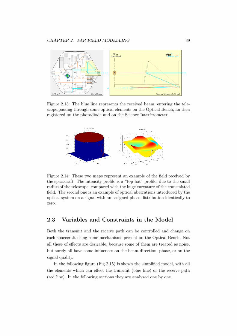
Figure 2.13: The blue line represents the received beam, entering the tele-scope,passing through some optical elements on the Optical Bench, an thenregistered on the photodiode and on the Science Interferometer.
Figure 2.14: These two maps represent an example of the field received bythe spacecraft. The intensity profile is a “top hat” profile, due to the smallradius of the telescope, compared with the huge curvature of the transmittedfield. The second one is an example of optical aberrations introduced by theoptical system on a signal with an assigned phase distribution identically tozero.
2.3 Variables and Constraints in the Model
Both the transmit and the receive path can be controlled and change oneach spacecraft using some mechanisms present on the Optical Bench. Notall these of effects are desirable, because some of them are treated as noise,but surely all have some influences on the beam direction, phase, or on thesignal quality.
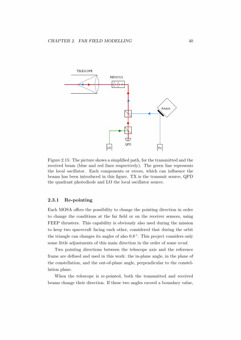
In the following figure (Fig.2.15) is shown the simplified model, with allthe elements which can effect the transmit (blue line) or the receive path(red line). In the following sections they are analyzed one by one.
CHAPTER 2. FAR FIELD MODELLING 40
Figure 2.15: The picture shows a simplified path, for the transmitted and thereceived beam (blue and red lines respectively). The green line representsthe local oscillator. Each components or errors, which can influence thebeams has been introduced in this figure. TX is the transmit source, QPDthe quadrant photodiode and LO the local oscillator source.
2.3.1 Re-pointing
Each MOSA offers the possibility to change the pointing direction in orderto change the conditions at the far field or on the receiver sensors, usingFEEP thrusters. This capability is obviously also used during the missionto keep two spacecraft facing each other, considered that during the orbitthe triangle can changes its angles of also 0.8 ◦. This project considers onlysome little adjustments of this main direction in the order of some nrad.
Two pointing directions between the telescope axis and the referenceframe are defined and used in this work: the in-plane angle, in the plane ofthe constellation, and the out-of-plane angle, perpendicular to the constel-lation plane.
When the telescope is re-pointed, both the transmitted and receivedbeams change their direction. If these two angles exceed a boundary value,

CHAPTER 2. FAR FIELD MODELLING 41
the quality of the received signal can be significantly reduced because theincoming wavefront tilt is too large to have a good resolution on the quad-rant photodiode. For this purpose an arbitrary boundary is imposed to thevariation of the angles:
−300nrad ≤ in plane angle ≤ 300nrad (2.34)
−300nrad ≤ out of plane angle ≤ 300nrad (2.35)
Figure 2.16: Effects of repointing the sending telescope on the phase slopeat the far field. The white circle is the position of the receiver telescope.
2.3.2 Refocus Mechanism
Despite the use of the pointing knowledge, the field wavefront quality at thefar field in the operating point is in general insufficient. For this reason aRefocus Mechanism is included in the telescope, able to change the weightof the fourth Zernike term (defocusing term). The mechanism is composedof three lenses, one of them movable in the beam axis direction. It influencesboth, the transmitted and the received beams, because both have to passthrough it.
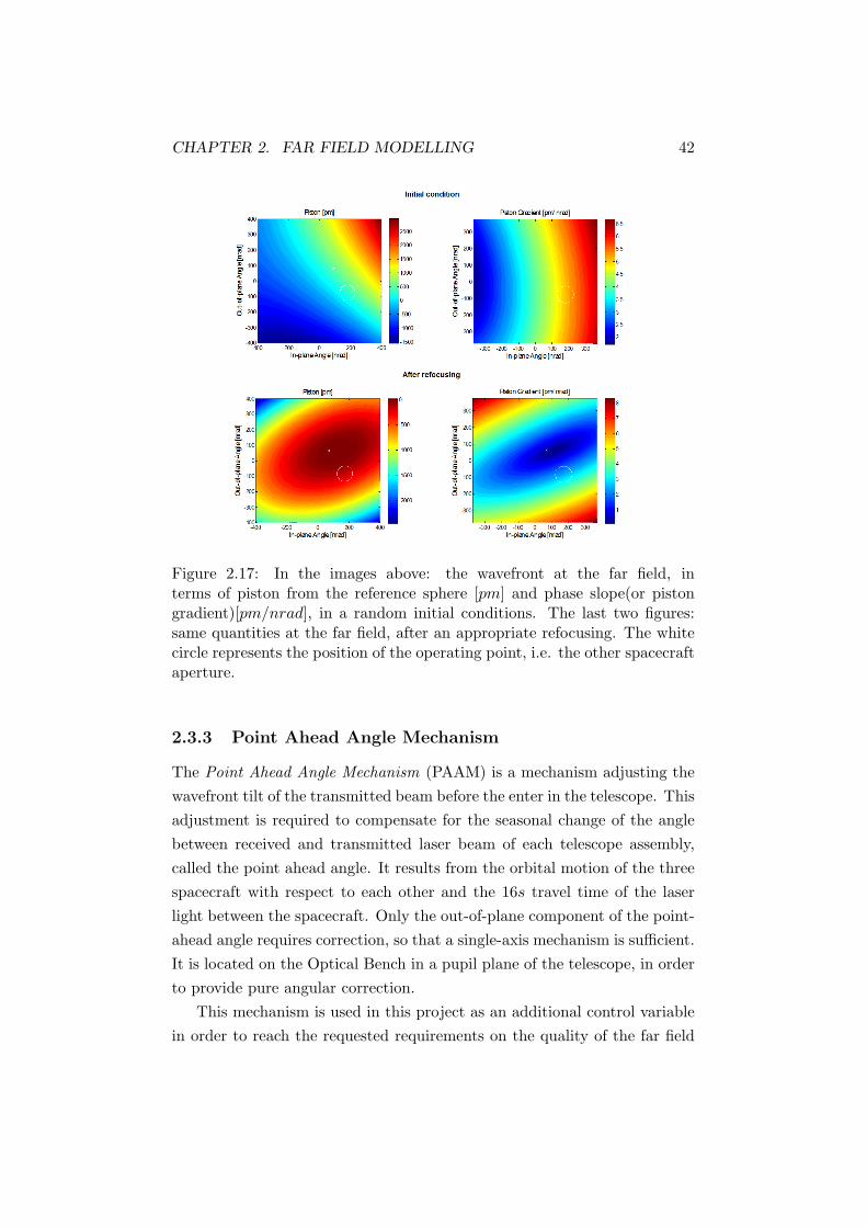
The main purpose of the refocusing, as intented within this project, isto minimize the wavefront phase slope at the far field in the operating pointand to reach a better quality of the signal on the quadrant photodiode.In Fig.2.17 the effects of refocusing on the wavefront at the far field areillustrated.
CHAPTER 2. FAR FIELD MODELLING 42
Figure 2.17: In the images above: the wavefront at the far field, interms of piston from the reference sphere [pm] and phase slope(or pistongradient)[pm/nrad], in a random initial conditions. The last two figures:same quantities at the far field, after an appropriate refocusing. The whitecircle represents the position of the operating point, i.e. the other spacecraftaperture.
2.3.3 Point Ahead Angle Mechanism
The Point Ahead Angle Mechanism (PAAM) is a mechanism adjusting thewavefront tilt of the transmitted beam before the enter in the telescope. Thisadjustment is required to compensate for the seasonal change of the anglebetween received and transmitted laser beam of each telescope assembly,called the point ahead angle. It results from the orbital motion of the threespacecraft with respect to each other and the 16s travel time of the laserlight between the spacecraft. Only the out-of-plane component of the point-ahead angle requires correction, so that a single-axis mechanism is sufficient.It is located on the Optical Bench in a pupil plane of the telescope, in orderto provide pure angular correction.
This mechanism is used in this project as an additional control variablein order to reach the requested requirements on the quality of the far field

CHAPTER 2. FAR FIELD MODELLING 43
wavefront and on the received signal. As its main purpose is to compensatethe misalignment between received and transmitted laser, only a small frac-tion of its range can be used for our purpose. So, in numerical terms, theconstraints on this variable can be translated as:
−300nrad ≤ out of plane anglePAAM ≤ 300nrad (2.36)
The effect of this mechanism is only on the transmit path, so only the farfield wavefront changes. Using a one-dimensional PAAM, the result is a shiftof the far field in the plane perpendicular to the spacecrafts constellation,as shown in Fig.2.18.
Figure 2.18: Effects of using PAAM on the far field wavefront. It correspondsto a vertical shift of the field.
2.3.4 Misalignment Errors
The model is defined to include some misalignment errors in the transmittedbeam direction: it is considered as the sum of all the mirror misalignment onthe Optical Bench and of the laser transmit source. In Fig.2.19 the dashedblue line represents the ideal transmit path, while the continuos blue line isan example of misaligned path.
For the position errors, all of them are referred to the pupil center whichis, in theory, coincident with the test mass center, considered to be thetransmit reference of the model. An offset between these two referencepoints is however included in the model, but not represented in this figure.
In the figure, instead, it is possible to see the offset in the plane per-pendicular to the beam of the transmit beam intensity profile (ideally a

CHAPTER 2. FAR FIELD MODELLING 44
Figure 2.19: Scheme of the model implemented, with the misalignment er-rors included in it.The red line represents the receive path, the blue dashedline the ideal transmit path and the continuous blue line the misalignedtransmit path. Also the shift of the intensity profiles and QPD position arerepresented.
Gaussian profile) from the pupil center.Also along the receive path there can be some position misalignments.
The location of the Quadrant Photodiode can be slightly shifted with respectto the pupil center while ideally the photodiode is exactly on it. Finally,the local oscillator, also referred to the pupil center, can have the inten-sity Gaussian profile not exactly centered in the plane perpendicular to thebeam direction. These misalignments influence the received signal and theheterodyne efficiency of the four quadrants.

Chapter 3
Algorithm for Long Arm
Interferometry Calibrations
The main goal of this project is to define a procedure for configuring twofaced telescopes of the one arm-interferometer, in order to obtain a goodsignal on the sensors and an acceptable wavefront quality at the far fieldin the operating position. To reach specific requirements, the control vari-ablesdescribed in Par.2.3 are available. The goal of this project is to findwhich values of these variables ensure good performance. The objective is astatistical study, depending on the Zernike distribution, expressed in term ofRMS wavefront error at the telescope pupil,in order to understand if the so-lution can always be similar to the optimum configuration. The distributionof the Zernike terms on the optical system depends on its manufacturingand technology so many different distributions are tested.
In this chapter the assumptions considered for the definition of the algo-rithm and an ideal optimization routine used as a benchmark for the nextalgorithm are presented.
3.1 Requirements
In this study the effects of the optical errors on the far field and on thereceived signal are defined as the contribution of each Zernike aberration, interms of RMS wavefront error on the telescope pupils.
For this project, the wavefront quality is connected with the piston gra-dient around the operating point at the far field: in fact, in case of jitter
45

CHAPTER 3. ALGORITHM FOR LONG ARM INTERFEROMETRY CALIBRATIONS46
of the sending telescope, always present for each MOSA, a small value ofthe phase slope ensures a quite stable value of the piston. In order to havean acceptable signal on the photodiode sensor, it is also necessary that theintensity received reaches a certain value, in order to distinguish the signalfrom the noise. Another quantity to keep under control is the heterodyneefficiency, defined in Par.2.1.3 on each quadrant of the photodiode: it isdepending on the power received (and then on the receiver position withrespect to the intensity peak location) and on the incoming wavefront tilt.So, the previous ideas can be translated in the following requirements:
phase slope ≤ 0.3pm/nrad
heterodyne efficiency ≥ 80%
received intensity ≥ 0.5 · intensity peak
These requirements can be reached by changing one or all the variablesdescribed in the Par.2.3(pointing angles, refocus wavefront error contributesand PAAM angles),in order to modify in some points the transmit or thereceive path. Some errors can be included in the algorithm to verify thestability of the system.
An important aspect that has been considered during this work is thenumber of measurements necessaries to reach the requirements. Each mea-surement taken to find the best configuration of the two telescopes corre-sponds to a calibration step. The data from the function evaluation needto be elaborated by the on ground computers and this procedure takes atleast one hour [7]. This aspect introduces a requirement in terms of num-ber of function evaluations used: this number need to be small, in order toconclude the calibration procedure in a reasonable amount of time.
3.2 Zernike Distribution
In this context the term ”weight vector” indicates a vector of eleven compo-nents which define the wavefront error contribution of the first eleven Zernikepolynomials at the telescope pupil. The term ”‘Zernike distribution”’ referto a specific set of weight vectors, which have some proprieties in terms ofwavefront error.

CHAPTER 3. ALGORITHM FOR LONG ARM INTERFEROMETRY CALIBRATIONS47
The RMS wavefront error at the telescope pupil is defined as:
wferms =12π
√√√√√∫ r0
−r0
∫√r20−y2
−√
r20−y2
Φ2(y, z) dz dy
πr20
(3.1)
where Φ is the Zernike field, that gives the distribution of the phase, asexplained in Par.2.1.1.
For the study different Zernike distributions are considered. The ideais to find which is the maximum wavefront error at the pupil that ensuresa good performance in a Montecarlo Simulation. The Zernike distributionstaken in account in this analysis are characterized by numerical values shownbelow.
For each of them, the wavefront error contribution of the initial refocusterm is given by:
wfermsZ4≤ λ/15rms (3.2)
This condition is valid for all cases. The distributions can be distinguishedfrom each other by the RMS wavefront error computed for the other terms,from the fifth to the eleventh. The following distributions are considered inthe study:
wferms(Z5−Z11)= λ/10rms (3.3)
wferms(Z5−Z11)= λ/15rms (3.4)
wferms(Z5−Z11)= λ/17rms (3.5)
wferms(Z5−Z11)= λ/20rms (3.6)
wferms(Z5−Z11)= λ/22rms (3.7)
wferms(Z5−Z11)= λ/25rms (3.8)
wferms(Z5−Z11)= λ/27rms (3.9)
wferms(Z5−Z11)= λ/30rms (3.10)
The weight vectors are generated in this way: the components from Z5
to Z11 are randomly created with the Matlab function rand. Then eachvector is scaled in order to find the set which gives the desired wavefronterror at the exit pupil. For each wavefront error hundreds of weight vectorhave been generated for the Montecarlo Simulation. Both telescopes have

CHAPTER 3. ALGORITHM FOR LONG ARM INTERFEROMETRY CALIBRATIONS48
some optical aberrations so, due to the symmetry of the interferometry, theresults of both of them are used for the same statistical analysis. Note thatdifferent sets of Zernike coefficients are used for the two telescopes, i.e. thetwo distributions are not correlated.
3.3 Starting conditions
In order to see the effects of the starting conditions, two different configu-rations for the telescope pointing directions have been taken into account.
The first one is the simplest geometrical configuration: the two telescopesface each others at the beginning of the calibration procedure, as shown inFig.3.1. They are directed along a geometrical reference line connecting thetwo proof masses of each spacecraft.
Figure 3.1: The two telescope, in this initial configuration,are pointed alongthe geometrical line connecting the respective proof masses at the beginningof the calibration procedure.
The second choice is to direct the two telescopes along the referencedirection that can be found from the on board sensors: the null direction inthe sense of the Differential Wavefront Sensing (see Par.2.2.5). This is theonly way possible to measure the orientation of the telescopes during thescience operation. So, as shown in the next figure (Fig.3.2), each of the twotelescopes, at the beginning of the calibration procedure is oriented alongthis direction.
The null direction depends on the optical characteristics of the receivertelescope but also on the conditions of the far field. Initially telescope T1 ispointed along the null direction and then telescope T2 directs itself along hisnull direction. At this point, the condition of the field received by telescopeT1 is theoretically changed (the far field changes when the telescope T2

CHAPTER 3. ALGORITHM FOR LONG ARM INTERFEROMETRY CALIBRATIONS49
Figure 3.2: The two telescope, in this initial configuration, are pointed alongthe the null direction at the beginning of the calibration procedure
re-points), but this effect is neglected in the model.
3.4 Ideal Optimization
As a preliminary analysis, an ideal optimization routine has been defined,as a benchmark, using standard optimization functions in Matlab. In thiscontext, the number of function evaluations needed is not important andthe only goal now is to find the best configuration.
For the definition of this benchmark algorithm, different strategies havebeen initially attempted. The behavior of these is briefly presented in Table3.4 but only the final one is presented in this text.
After a brief initial analysis it is resulted that, for this model, it is quiteeasy to reach a good heterodyne efficiency of the two quadrant photodiodesif the pointing directions of the two telescopes are not too far from the nulldirection. However it seems to be more complicated to reach a good valuefor the piston gradient in the operating point for all cases. For this reason,an initial maximization of the heterodyne efficiency is followed by manyattempts to minimize the piston gradient at the operating point.
The code proceeds in the following way:
1. Maximization of heterodyne efficiency on the two telescopes, by chang-ing the refocus wavefront error contributions on both;
2. Minimization of piston gradient at the operating point, using the point-ing angles. Before moves T1, then moves T2;
3. Minimization of piston gradient at the operating point, using the

CHAPTER 3. ALGORITHM FOR LONG ARM INTERFEROMETRY CALIBRATIONS50
Stra
tegy
Pro
Con
Min
pist
ongr
adie
nt-
refo
cus
Onl
yon
efu
ncti
onev
alua
tion
nece
ssar
yto
redu
ceth
epi
ston
grad
ient
wit
hth
ere
focu
s
Wit
hon
lyth
isat
tem
pts,
the
pist
ongr
adie
ntre
ache
sth
ere
quir
emen
tsre
ques
ted
inve
ryfe
wca
ses.
The
hete
rody
neeffi
cien
cyis
hard
tom
axim
ize
wit
hth
eon
lyre
-poi
ntin
g
Max
hete
rody
neeffi
cien
cy-
poin
ting
Min
pist
ongr
adie
nt-
refo
cus
and
re-p
oint
ing
Qui
teea
syto
ente
rth
ere
quir
emen
tsin
term
sof
pist
ongr
adie
nt.
Not
too
man
yfu
ncti
onev
alua
tion
sne
eded
Whi
lere
-poi
ntin
g(o
rus
ing
refo
cus
mec
hani
sm)
for
max
imiz
ing
the
hete
rody
neeffi
cien
cy,th
epi
ston
grad
ient
incr
emen
tis
not
acce
ptab
le
Max
hete
rody
neeffi
cien
cy-
poin
ting
(or
refo
cus)
Max
hete
rody
neeffi
cien
cy-
refo
cus
Het
erod
yne
effici
ency
decr
emen
tsdu
eto
min
imiz
atio
nof
pist
ongr
adie
ntar
eac
cept
able
.P
isto
ngr
adie
ntca
nen
ter
the
requ
irem
ents
inm
ost
ofth
eca
ses
Man
yfu
ncti
onev
alua
tion
sne
eded
.M
any
opti
miz
atio
nst
eps
need
edto
redu
ceth
epi
ston
grad
ient
Min
pist
ongr
adie
nt-
poin
ting
,PA
AM
,re
focu
s
Tab
le3.
1:A
dvan
tage
san
ddi
sadv
anta
ges
ofdi
ffere
ntst
rate
gies
for
the
idea
lop
tim
izat
ion.

CHAPTER 3. ALGORITHM FOR LONG ARM INTERFEROMETRY CALIBRATIONS51
PAAM angles. Before changes PAAM angle on T1, then on T2;
4. Minimization of piston gradient at the operating point, using the re-focus mechanism. Before before changes refocus on T1, the on T2.
For maximizing the heterodyne efficiency the code uses the refocus wave-front error contribution: in this part, the value of wferef is changed on bothtelescopes. In this way, also the far field changes in the two directions. Thegoal of the code after this first step is to move the far field associated withthe two telescopes to minimize the piston gradient value at the operatingpoint (it considers now one telescope per time). In order to do this, the algo-rithm changes sequentially the pointing direction, the PAAM angle and therefocus wavefront error contribution. A variation in the pointing directionof the telescope and in the refocus wavefront error contribution effects thetransmit but also the received path. The PAAM angle, however effects onlythe transmitted beam so it can be useful where the heterodyne efficiency isa critical parameter.
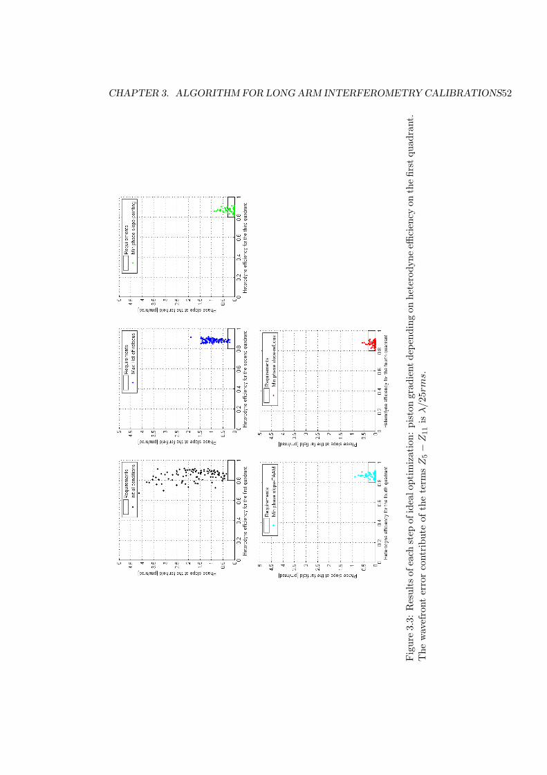
An example of the results obtained with this optimization is depictedin Fig.3.3. In this case, 100 weight vectors per telescope are randomlygenerated: for all of them the contribution at the wavefront error of theZernike polynomials from Z5 to Z11 is λ/25rms. In the figure, each stepis represented in a single plot: first the maximization of the heterodyneefficiency using the refocus mechanism, then the minimization of the pistongradient at the operating point using the pointing direction, the PAAMangle, and the refocus mechanism.
This approach is clearly not feasible in the mission: each cases needsmore or less 150 function evaluations to find the best solution. In a realcalibration process this could means many days of measurements and dataprocessing to arrive at the same result.
CHAPTER 3. ALGORITHM FOR LONG ARM INTERFEROMETRY CALIBRATIONS52
Fig
ure
3.3:
Res
ults
ofea
chst
epof
idea
lopt
imiz
atio
n:pi
ston
grad
ient
depe
ndin
gon
hete
rody
neeffi
cien
cyon
the
first
quad
rant
.T
hew
avef
ront
erro
rco
ntri
bute
ofth
ete
rms
Z5−
Z11
isλ/25
rms.
Chapter 4
Optimization Algorithm
In this chapter the algorithm found for the optimization of the performancefor one arm of the interferometer is presented. The quantities controlled arethe phase slope at the far field operating point and the heterodyne efficiencyon the quadrant photodiode.
Below a first approach to the problem is presented, which uses only thepointing angles and the refocus value as control variables, and for now ne-glects the PAAM out-of-plane angle. At the end of this chapter, it is pointedout how to introduce the PAAM out-of-plane angle for some solutions.
Not only has the algorithm to find the better set of parameters for eachZernike polynomial weight vector randomly generated, but also during thisprocedure, it has to use a minimum number of function evaluations. As pre-viously explained, each function evaluation at the far field operating pointneeds, due to on-ground data processing, about one hour for the measure-ments [7].
4.1 Approximations Considered
The algorithm tries to rebuild the real field from a small number of func-tion evaluations. Using the measurements taken in some points, it findsapproximated expressions for the piston gradient at the far field and theheterodyne efficiency on the four quadrants, which are used to define thebest configuration of the control variables. In the paragraphs below, someconsiderations are pointed out about the approximations used in the code.
53
CHAPTER 4. OPTIMIZATION ALGORITHM 54
4.1.1 Refocus Effect on Piston Gradient at the Far Field and
Heterodyne Efficiency
In order to define a good strategy for the optimization algorithm, it is nec-essary to analyse the effect of the control variables on the quantities ofinterest. The refocus value is a real important control variable: it is quiteeasy to change and it strongly effects both the far field, in term of pistonand piston gradient, and the heterodyne efficiency on the receive path.
In order to have an idea of the results of refocusing at the far field, seeFig.2.17. The effect of refocusing on the far field is clear considering an idealtelescope, in which the only contribution at the phase distribution is due tothe refocus, in terms of Zernike polynomials (in Fig.4.1 there are the effectson the piston and on the piston gradient).
The piston at the far field can be approximated, with a good precision,with an elliptic paraboloid.
Figure 4.1: Effect of refocus (considering an ideal sending telescope withZi = 0, i = 5..11) on the piston and piston gradient far field. Both quantitiesare referred to the reference sphere of 5 million kilometers radius.
The effect of the refocus, (considering an ideal telescope) on the pistonand the piston gradient can be written as:
pref (wferef , φy, φz) = −wferef · 1017 · (φ2y + φ2
z) (4.1)
gradpref (wferef , φy, φz) = |wferef | · 108 ·√
φ2y + φ2
z (4.2)
where pref is expressed in pm and gradpref in pm/nrad. The variableswferef is the RMS wavefront error associated with the fourth Zernike poly-nomial (the refocus term). In Fig.4.2 are displayed the real and the approx-

CHAPTER 4. OPTIMIZATION ALGORITHM 55
imated piston and piston gradient at the operating point, as functions ofwferef .
Figure 4.2: Plots refer to the operating point (randomly chosen). The redplots represents the real dependence between the conditions at the far fieldand the wavefront error depending on the refocus value, the blue lines arethe approximated functions. The two plots belows show the absolute error.
From the approximated functions, it is possible to establish an approxi-mated value for the refocus weight contribution which minimizes the pistongradient at the operating point. For doing this, it is considered that the ef-fect of the only refocus can be added to the real field at the operating point.In practice, there are two fields, propagating with the function expressedin Eq.2.23: one is the initial beam, with its own Zernike distribution ΦZ ,and the other one is the refocus effect, where the Zernike polynomial onlyhas the refocus term, and add them in the operating point. The Zernikepolynomials are orthonormal functions on the unit circle so this operationis always valid.
Then, to minimize the piston gradient in the operating point using the
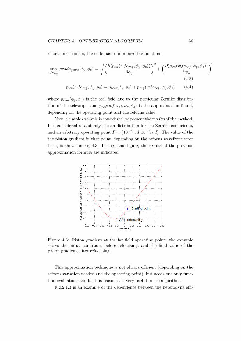
CHAPTER 4. OPTIMIZATION ALGORITHM 56
refocus mechanism, the code has to minimize the function:
minwferef
gradpfinal(φy, φz) =
√(∂(ptot(wferef , φy, φz))
∂φy
)2
+(
∂(ptot(wferef , φy, φz))∂φz
)2
(4.3)
ptot(wferef , φy, φz) = preal(φy, φz) + pref (wferef , φy, φz) (4.4)
where preal(φy, φz) is the real field due to the particular Zernike distribu-tion of the telescope, and pref (wferef , φy, φz) is the approximation found,depending on the operating point and the refocus value.
Now, a simple example is considered, to present the results of the method.It is considered a randomly chosen distribution for the Zernike coefficients,and an arbitrary operating point P = (10−7rad, 10−7rad). The value of thethe piston gradient in that point, depending on the refocus wavefront errorterm, is shown in Fig.4.3. In the same figure, the results of the previousapproximation formula are indicated.
Figure 4.3: Piston gradient at the far field operating point: the exampleshows the initial condition, before refocusing, and the final value of thepiston gradient, after refocusing.
This approximation technique is not always efficient (depending on therefocus variation needed and the operating point), but needs one only func-tion evaluation, and for this reason it is very useful in the algorithm.
Fig.2.1.3 is an example of the dependence between the heterodyne effi-

CHAPTER 4. OPTIMIZATION ALGORITHM 57
ciency on the four quadrant and the refocus value on the receive path, forrandomly chosen Zernike weight vectors and incoming wavefront tilts.
Figure 4.4: Heterodyne efficiency on the four quadrants of the photodiode,as a function of the refocus weight value, for a randomly chosen Zernikedistribution. The dashed black line is the requirements of the project (80%).
As each plot in Fig.2.1.3 is similar to a parabola, the code use threefunction evaluations to approximate the real function. In this way, it canwork with four known functions and find the maximum of each of them.In the next figure (Fig.4.5) the real function and the approximated one areshown , with the position where the measurements have been taken.
4.1.2 Pointing Angles Effect on Piston Gradient at the Far
Field and the Heterodyne Efficiency
For the far field piston gradient, a variation of the pointing direction of thetelescope corresponds to a respective movement of the field on the referencesphere. The field in practice does not change: there is a movement of theoperating point on the reference sphere.

CHAPTER 4. OPTIMIZATION ALGORITHM 58
Figure 4.5: Real (red plots) and approximated (blue plots) heterodyne effi-ciencies on the four quadrants of the photodiode. The black circles are themeasurements used for the approximation.
In order to reduce the number of function evaluations needed to find theminimum piston gradient in the far field, an approximation of the field isused. As done previously with the heterodyne efficiency, the field dependingon the position can be estimated with a certain number of measurements. Asit always has a minimum, the approximated field is expressed as a paraboloidwith the form:
gradpapprox := aφ2y + bφ2
z + cφy + dφz + e (4.5)
where a, b, c, d, e are parameters to be defined from the measurements takenin 5 points (the minimum number of function evaluations necessary). InFig.4.6 there is as example of the far field piston gradient approximationresults: the starting position now is in the point (0, 0): four additionalmeasurements are taken around this one. From this, the new approximatedfield, shown also in the figure, is evaluated.
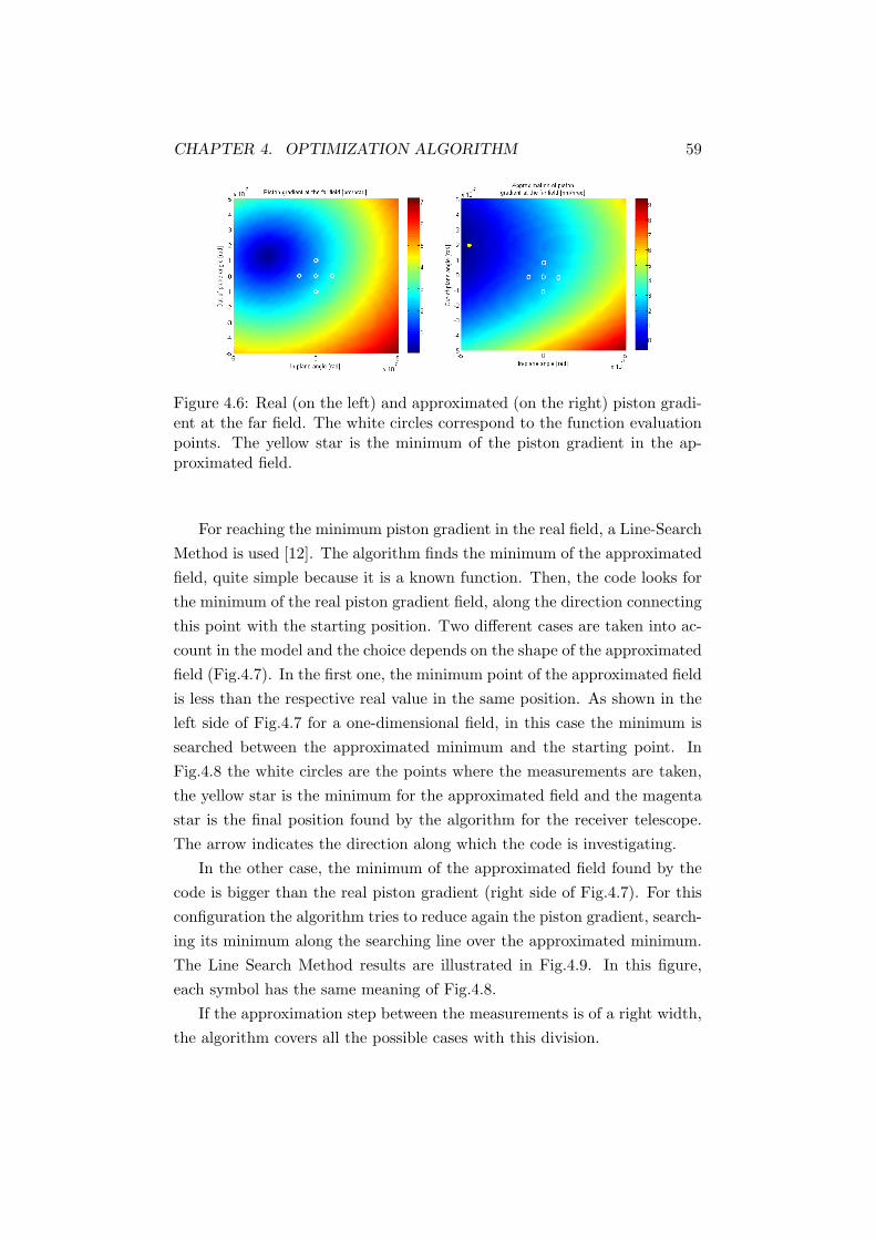
CHAPTER 4. OPTIMIZATION ALGORITHM 59
Figure 4.6: Real (on the left) and approximated (on the right) piston gradi-ent at the far field. The white circles correspond to the function evaluationpoints. The yellow star is the minimum of the piston gradient in the ap-proximated field.
For reaching the minimum piston gradient in the real field, a Line-SearchMethod is used [12]. The algorithm finds the minimum of the approximatedfield, quite simple because it is a known function. Then, the code looks forthe minimum of the real piston gradient field, along the direction connectingthis point with the starting position. Two different cases are taken into ac-count in the model and the choice depends on the shape of the approximatedfield (Fig.4.7). In the first one, the minimum point of the approximated fieldis less than the respective real value in the same position. As shown in theleft side of Fig.4.7 for a one-dimensional field, in this case the minimum issearched between the approximated minimum and the starting point. InFig.4.8 the white circles are the points where the measurements are taken,the yellow star is the minimum for the approximated field and the magentastar is the final position found by the algorithm for the receiver telescope.The arrow indicates the direction along which the code is investigating.
In the other case, the minimum of the approximated field found by thecode is bigger than the real piston gradient (right side of Fig.4.7). For thisconfiguration the algorithm tries to reduce again the piston gradient, search-ing its minimum along the searching line over the approximated minimum.The Line Search Method results are illustrated in Fig.4.9. In this figure,each symbol has the same meaning of Fig.4.8.
If the approximation step between the measurements is of a right width,the algorithm covers all the possible cases with this division.

CHAPTER 4. OPTIMIZATION ALGORITHM 60
Figure 4.7: Real and approximated piston gradient: two cases for the algo-rithm line search method. the arrow is the direction of the searching line.
For the heterodyne efficiency in the receiver telescope, the situation is abit more complex. If the sending telescope T1 changes its pointing direction,the incoming wavefront tilt in telescope T2 changes also, due to the opticalaberrations on the wavefront. Obviously, if T2 changes its direction, theincoming wavefront tilt has a variation. This effect in the receive path ismuch more significant (at least four order of magnitude).
The heterodyne efficiency in this last case is quite sensitive. A good pa-rameter for the definition of a correct direction is the null direction (Par.2.2.5):too far from this direction, the heterodyne efficiency is too low for havingan acceptable signal on the quadrant photodiode. In Fig.4.10 this effectis represented. The telescope is pointing along the null direction in theplane perpendicular to the constellation but the in-plane angle change con-tinuously in the range of µrad. The circles in the figure are the real nulldirection in the plane of the constellation. The green area represents thevariation range of the in-plane angle accepted in the algorithm. The samerange is used for the out-of-plane angle.
For now a wider variation range for the pointing angles, with respect towhat introduced in Par.2.3.1, is considered, as shown in Fig.4.10:
−450nrad ≤ in plane angle ≤ 450nrad (4.6)
−450nrad ≤ out of plane angle ≤ 450nrad (4.7)
This choice is motivated by the analysis of the previous plots, in whicha wider range still admits a good heterodyne efficiency and by the fact thatfor now, the PAAM out-of-plane angle is not used. Then, a wider but always

CHAPTER 4. OPTIMIZATION ALGORITHM 61
Figure 4.8: The two plots on the left side represent the real piston gradi-ent and the approximated one. The white circles are the points where themeasurements are taken: the yellow star is the minimum point of the ap-proximated field and the magenta star the solution found by the algorithmfor this particular case.
limited range gives more freedom in the search of the best configuration.
4.2 Strategy
From the previous analysis and the results of the ideal optimization, illus-trated in Par.3.4, a strategy has been defined for the final algorithm. Asexplained before, this routine does not foresee to use the PAAM out-of-planeangle, but only the pointing angles and the refocus mechanism of the twotelescopes. A second approach, which comprises the PAAM out-of-planeangle, is presented at the end of this paragraph, as a possible solution forsome cases of excess errors found during the project.
The code proceeds in this way:
1. Maximization of heterodyne efficiency using Refocusing Mechanismon both telescope. The code builds approximations of the heterodyne

CHAPTER 4. OPTIMIZATION ALGORITHM 62
Figure 4.9: The two plots on the left side represent the real piston gradi-ent and the approximated one. The white circles are the points where themeasurements are taken: the yellow star is the minimum point of the ap-proximated field and the magenta star the solution found by the algorithmfor this particular case.
efficiency functions and finds the best refocus values;
2. Minimization of piston gradient: before for telescope T1, then fortelescope T2. The algorithm tries to re-point the telescope: it buildsan approximation of the far field piston gradient and uses the LineSearch Method;
3. Minimization of piston gradient: if with the previous step the require-ments in terms of piston gradient are not reached, it uses the RefocusMechanism to minimize it, with the analytical formulation of Par.4.1.1;
4. If piston gradient is not in the requirements, the code repeats step 2and step 3.
First of all, the refocus mechanisms of the two telescope are used to max-imize the heterodyne efficiency on the photodiode of each MOSA. Changing

CHAPTER 4. OPTIMIZATION ALGORITHM 63
Figure 4.10: Variation of the heterodyne efficiency in the four quadrantsof the photodiode, depending on the in-plane angle. The circles are theconditions along the null direction. The green area is the variation rangeused in the algorithm for the in-plane angle.
the refocus wavefront error contribution for maximizing the efficiency onT1, also the far field changes at the operating point, and then the incomingwavefront tilt at the receiver telescope T2. So, in principle, the hetero-dyne efficiency, for example on T2 depends on the refocus value of bothtelescopes (sender T1 and receiver T2). In fact the heterodyne efficiency isreally slightly depending on the refocus value of the sender telescope, so thiseffect is neglected, and it is referred only to the refocus value in the receivepath as previously done with the plots in Figg.2.1.3-4.5.
The algorithm considers for the searching of the maximum efficiencypoint only one parabola obtained as the sum of the four parabolas of thequadrants. In this way, what actually is maximized is the ”efficiency mean”on the four quadrants. In the next figures (Figg.4.11-4.12) the results ofthis first step are represented, on the heterodyne efficiency, and on the the

CHAPTER 4. OPTIMIZATION ALGORITHM 64
piston gradient at the far field. As can be seen, the heterodyne efficiency onthe first quadrant at the end is less than the initial value, but in total thesituation is significantly better.
Figure 4.11: Heterodyne efficiency depending on the refocus value. Thecircle is the initial refocus value, the star marker is the final one, after thefirst optimization step.
During the heterodyne efficiency maximization also the far field pistongradient changes: but for now only the receive path is taken into account, sothe position of the other telescope on the reference sphere is not considered.
In the second step, the algorithm considers how to minimize the pistongradient at the operating point for the both telescopes. The code changes thepointing angles and the refocus wavefront error contribution of the sendingtelescope in order to bring the receiver telescope in the requirements. Theseoperations are done sequentially, first for one telescope and then for thesecond one.
The algorithm, from its starting position, defines an approximated field,taking another four measurements around the initial one, and tries to reach
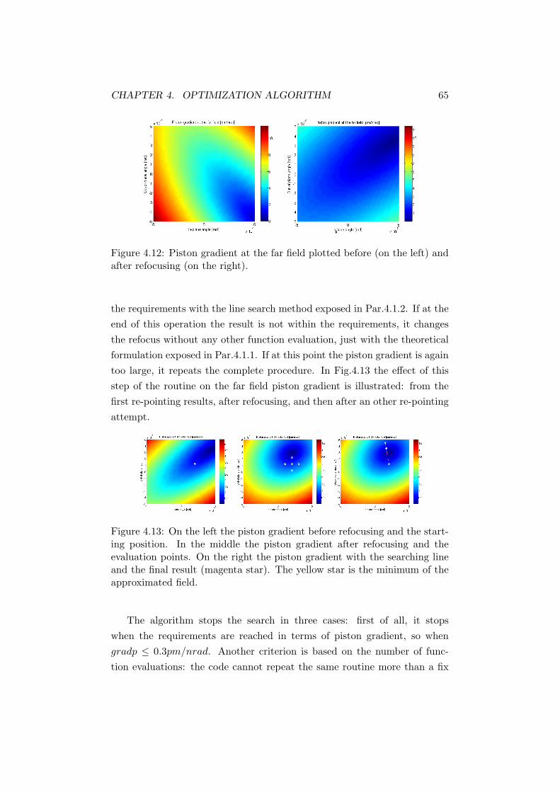
CHAPTER 4. OPTIMIZATION ALGORITHM 65
Figure 4.12: Piston gradient at the far field plotted before (on the left) andafter refocusing (on the right).
the requirements with the line search method exposed in Par.4.1.2. If at theend of this operation the result is not within the requirements, it changesthe refocus without any other function evaluation, just with the theoreticalformulation exposed in Par.4.1.1. If at this point the piston gradient is againtoo large, it repeats the complete procedure. In Fig.4.13 the effect of thisstep of the routine on the far field piston gradient is illustrated: from thefirst re-pointing results, after refocusing, and then after an other re-pointingattempt.
Figure 4.13: On the left the piston gradient before refocusing and the start-ing position. In the middle the piston gradient after refocusing and theevaluation points. On the right the piston gradient with the searching lineand the final result (magenta star). The yellow star is the minimum of theapproximated field.
The algorithm stops the search in three cases: first of all, it stopswhen the requirements are reached in terms of piston gradient, so whengradp ≤ 0.3pm/nrad. Another criterion is based on the number of func-tion evaluations: the code cannot repeat the same routine more than a fix
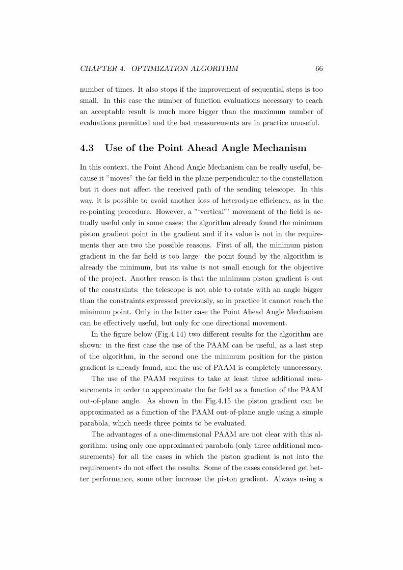
CHAPTER 4. OPTIMIZATION ALGORITHM 66
number of times. It also stops if the improvement of sequential steps is toosmall. In this case the number of function evaluations necessary to reachan acceptable result is much more bigger than the maximum number ofevaluations permitted and the last measurements are in practice unuseful.
4.3 Use of the Point Ahead Angle Mechanism
In this context, the Point Ahead Angle Mechanism can be really useful, be-cause it ”moves” the far field in the plane perpendicular to the constellationbut it does not affect the received path of the sending telescope. In thisway, it is possible to avoid another loss of heterodyne efficiency, as in there-pointing procedure. However, a ”‘vertical”’ movement of the field is ac-tually useful only in some cases: the algorithm already found the minimumpiston gradient point in the gradient and if its value is not in the require-ments ther are two the possible reasons. First of all, the minimum pistongradient in the far field is too large: the point found by the algorithm isalready the minimum, but its value is not small enough for the objectiveof the project. Another reason is that the minimum piston gradient is outof the constraints: the telescope is not able to rotate with an angle biggerthan the constraints expressed previously, so in practice it cannot reach theminimum point. Only in the latter case the Point Ahead Angle Mechanismcan be effectively useful, but only for one directional movement.
In the figure below (Fig.4.14) two different results for the algorithm areshown: in the first case the use of the PAAM can be useful, as a last stepof the algorithm, in the second one the minimum position for the pistongradient is already found, and the use of PAAM is completely unnecessary.
The use of the PAAM requires to take at least three additional mea-surements in order to approximate the far field as a function of the PAAMout-of-plane angle. As shown in the Fig.4.15 the piston gradient can beapproximated as a function of the PAAM out-of-plane angle using a simpleparabola, which needs three points to be evaluated.
The advantages of a one-dimensional PAAM are not clear with this al-gorithm: using only one approximated parabola (only three additional mea-surements) for all the cases in which the piston gradient is not into therequirements do not effect the results. Some of the cases considered get bet-ter performance, some other increase the piston gradient. Always using a

CHAPTER 4. OPTIMIZATION ALGORITHM 67
Figure 4.14: Two results of the algorithm: on the left side the minimumpiston gradient is out of the constrains, on the right side the algorithm findsthe minimum is in the constraints, but too big for the requirements.
one-dimensional PAAM, a different approach to the problem can be tested,building more approximated parabolas, in order to have a better estimationof the real field. Each parabola need obviously three more measurements.A two-dimensional PAAM can also be tested, considering that the approxi-mation of a two-dimensional field needs at least five function evaluations.

CHAPTER 4. OPTIMIZATION ALGORITHM 68
Figure 4.15: The red plot is the real piston gradient at the operating pointdepending on the PAAM out-of-plane angle. The blue plot is the approx-imated parabola. The three black circles correspond to the measurementpoints.

Chapter 5
Results
The algorithm has been used with two different starting conditions as ex-plained in Par.3.3. In order to have a complete statistical study for realistictelescopes, different Zernike distributions have been considered, as describedin Par.3.2. For each Zernike wavefront error considered, 100 cases per tele-scope have been randomly generated. The interferometry is completely sym-metrical, so 200 cases are in practice the base for each Montecarlo Simula-tion. In the following pictures the results of the algorithm for each differentwavefront error distribution and both the starting conditions are presented.
5.1 Results for different Zernike Distributions
5.1.1 Starting condition: along geometrical direction
The results show the piston gradient at the far field, in term of pm/nrad,depending on the heterodyne efficiency on the four quadrants. In order toconsider all the results, the data from telescope T1 and telescope T2 are puttogether in these figures (from the symmetry of the interferometry this actiondoes not imply any loss of precision). In each picture are also drawn therequirements in terms of heterodyne efficiency and piston gradient. The bluepoints are the intermediate results, after the maximization of the heterodyneefficiency, the red points are the last results of the algorithm. The aim ofthe algorithm is to reach the rectangle in the low corner with the all redpoints. Figg.5.9 and 5.10 represent the frequencies of the results, Table5.1.1shows the main statistical values obtained in each case.
69

CHAPTER 5. RESULTS 70
Fig
ure
5.1:
Res
ults
:st
arti
ngco
ndit
ion
wit
hte
lesc
opes
dire
cted
alon
gge
omet
rica
llin
e,w
avef
ront
erro
rZ
5−
Z11
=λ/10
rms.
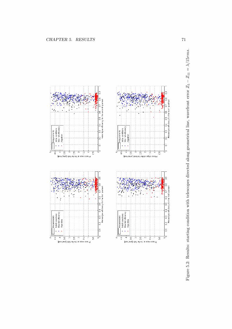
CHAPTER 5. RESULTS 71
Fig
ure
5.2:
Res
ults
:st
arti
ngco
ndit
ion
wit
hte
lesc
opes
dire
cted
alon
gge
omet
rica
llin
e,w
avef
ront
erro
rZ
5−
Z11
=λ/15
rms.

CHAPTER 5. RESULTS 72
Fig
ure
5.3:
Res
ults
:st
arti
ngco
ndit
ion
wit
hte
lesc
opes
dire
cted
alon
gge
omet
rica
llin
e,w
avef
ront
erro
rZ
5−
Z11
=λ/17
rms.

CHAPTER 5. RESULTS 73
Fig
ure
5.4:
Res
ults
:st
arti
ngco
ndit
ion
wit
hte
lesc
opes
dire
cted
alon
gge
omet
rica
llin
e,w
avef
ront
erro
rZ
5−
Z11
=λ/20
rms.

CHAPTER 5. RESULTS 74
Fig
ure
5.5:
Res
ults
:st
arti
ngco
ndit
ion
wit
hte
lesc
opes
dire
cted
alon
gge
omet
rica
llin
e,w
avef
ront
erro
rZ
5−
Z11
=λ/22
rms.

CHAPTER 5. RESULTS 75
Fig
ure
5.6:
Res
ults
:st
arti
ngco
ndit
ion
wit
hte
lesc
opes
dire
cted
alon
gge
omet
rica
llin
e,w
avef
ront
erro
rZ
5−
Z11
=λ/25
rms.

CHAPTER 5. RESULTS 76
Fig
ure
5.7:
Res
ults
:st
arti
ngco
ndit
ion
wit
hte
lesc
opes
dire
cted
alon
gge
omet
rica
llin
e,w
avef
ront
erro
rZ
5−
Z11
=λ/27
rms.

CHAPTER 5. RESULTS 77
Fig
ure
5.8:
Res
ults
:st
arti
ngco
ndit
ion
wit
hte
lesc
opes
dire
cted
alon
gge
omet
rica
llin
e,w
avef
ront
erro
rZ
5−
Z11
=λ/30
rms.

CHAPTER 5. RESULTS 78
Figure 5.9: Frequency of heterodyne efficiency values (all quadrants consid-ered) for all the Zernike distributions tested. Initial condition: telescopesdirected along the geometrical line connecting the two test masses
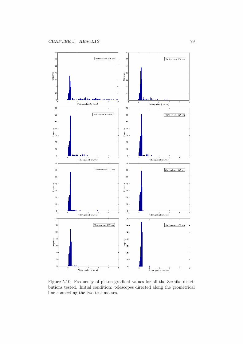
CHAPTER 5. RESULTS 79
Figure 5.10: Frequency of piston gradient values for all the Zernike distri-butions tested. Initial condition: telescopes directed along the geometricalline connecting the two test masses.
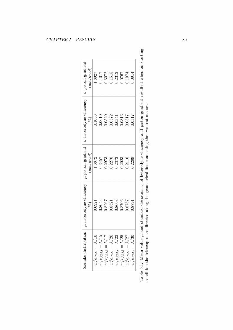
CHAPTER 5. RESULTS 80
Zer
nike
dist
ribu
tion
µhe
tero
dyne
effici
ency
µpi
ston
grad
ient
σhe
tero
dyne
effici
ency
σpi
ston
grad
ient
(%)
(pm
/nra
d)
(%)
(pm
/nra
d)
wfe R
MS
=λ/10
0.69
211.
3872
0.10
331.
8927
wfe R
MS
=λ/15
0.80
430.
3457
0.06
100.
4017
wfe R
MS
=λ/17
0.82
670.
2973
0.05
200.
3072
wfe R
MS
=λ/20
0.85
210.
2270
0.03
720.
1515
wfe R
MS
=λ/22
0.86
080.
2373
0.03
410.
2312
wfe R
MS
=λ/25
0.87
060.
2023
0.03
160.
0767
wfe R
MS
=λ/27
0.87
570.
2110
0.03
170.
1074
wfe R
MS
=λ/30
0.87
910.
2209
0.03
170.
0914
Tab
le5.
1:M
ean
valu
eµ
and
stan
dard
devi
atio
nσ
ofhe
tero
dyne
effici
ency
and
pist
ongr
adie
ntre
sult
edw
hen
asst
arti
ngco
ndit
ion
the
tele
scop
esar
edi
rect
edal
ong
the
geom
etri
callin
eco
nnec
ting
the
two
test
mas
ses.
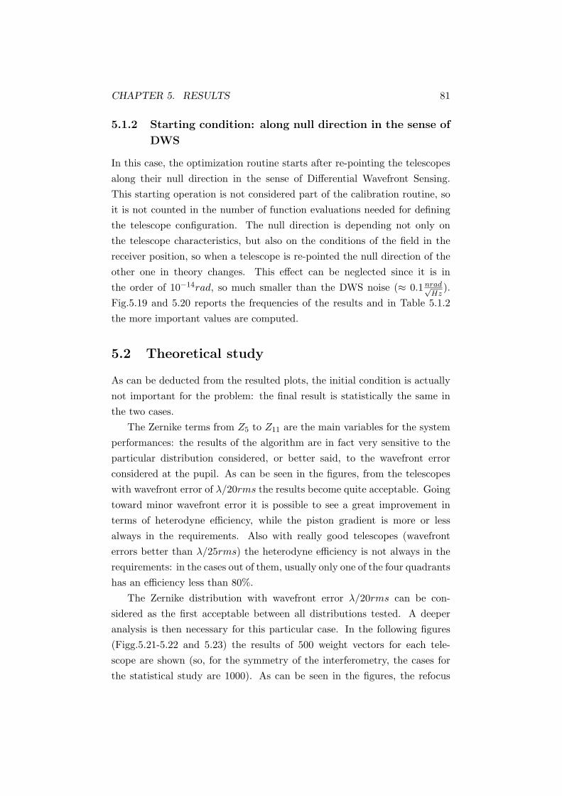
CHAPTER 5. RESULTS 81
5.1.2 Starting condition: along null direction in the sense of
DWS
In this case, the optimization routine starts after re-pointing the telescopesalong their null direction in the sense of Differential Wavefront Sensing.This starting operation is not considered part of the calibration routine, soit is not counted in the number of function evaluations needed for definingthe telescope configuration. The null direction is depending not only onthe telescope characteristics, but also on the conditions of the field in thereceiver position, so when a telescope is re-pointed the null direction of theother one in theory changes. This effect can be neglected since it is inthe order of 10−14rad, so much smaller than the DWS noise (≈ 0.1 nrad√
Hz).
Fig.5.19 and 5.20 reports the frequencies of the results and in Table 5.1.2the more important values are computed.
5.2 Theoretical study
As can be deducted from the resulted plots, the initial condition is actuallynot important for the problem: the final result is statistically the same inthe two cases.
The Zernike terms from Z5 to Z11 are the main variables for the systemperformances: the results of the algorithm are in fact very sensitive to theparticular distribution considered, or better said, to the wavefront errorconsidered at the pupil. As can be seen in the figures, from the telescopeswith wavefront error of λ/20rms the results become quite acceptable. Goingtoward minor wavefront error it is possible to see a great improvement interms of heterodyne efficiency, while the piston gradient is more or lessalways in the requirements. Also with really good telescopes (wavefronterrors better than λ/25rms) the heterodyne efficiency is not always in therequirements: in the cases out of them, usually only one of the four quadrantshas an efficiency less than 80%.
The Zernike distribution with wavefront error λ/20rms can be con-sidered as the first acceptable between all distributions tested. A deeperanalysis is then necessary for this particular case. In the following figures(Figg.5.21-5.22 and 5.23) the results of 500 weight vectors for each tele-scope are shown (so, for the symmetry of the interferometry, the cases forthe statistical study are 1000). As can be seen in the figures, the refocus

CHAPTER 5. RESULTS 82
Fig
ure
5.11
:R
esul
ts:
star
ting
cond
itio
nw
ith
tele
scop
esdi
rect
edal
ong
null
dire
ctio
n,w
avef
ront
erro
rZ
5−
Z11
=λ/10
rms.

CHAPTER 5. RESULTS 83
Fig
ure
5.12
:R
esul
ts:
star
ting
cond
itio
nw
ith
tele
scop
esdi
rect
edal
ong
null
dire
ctio
n,w
avef
ront
erro
rZ
5−
Z11
=λ/15
rms.

CHAPTER 5. RESULTS 84
Fig
ure
5.13
:R
esul
ts:
star
ting
cond
itio
nw
ith
tele
scop
esdi
rect
edal
ong
null
dire
ctio
n,w
avef
ront
erro
rZ
5−
Z11
=λ/17
rms.

CHAPTER 5. RESULTS 85
Fig
ure
5.14
:R
esul
ts:
star
ting
cond
itio
nw
ith
tele
scop
esdi
rect
edal
ong
null
dire
ctio
n,w
avef
ront
erro
rZ
5−
Z11
=λ/20
rms.

CHAPTER 5. RESULTS 86
Fig
ure
5.15
:R
esul
ts:
star
ting
cond
itio
nw
ith
tele
scop
esdi
rect
edal
ong
null
dire
ctio
n,w
avef
ront
erro
rZ
5−
Z11
=λ/22
rms.

CHAPTER 5. RESULTS 87
Fig
ure
5.16
:R
esul
ts:
star
ting
cond
itio
nw
ith
tele
scop
esdi
rect
edal
ong
null
dire
ctio
n,w
avef
ront
erro
rZ
5−
Z11
=λ/25
rms.
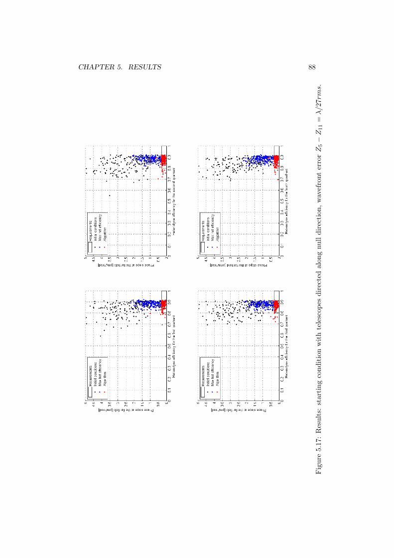
CHAPTER 5. RESULTS 88
Fig
ure
5.17
:R
esul
ts:
star
ting
cond
itio
nw
ith
tele
scop
esdi
rect
edal
ong
null
dire
ctio
n,w
avef
ront
erro
rZ
5−
Z11
=λ/27
rms.
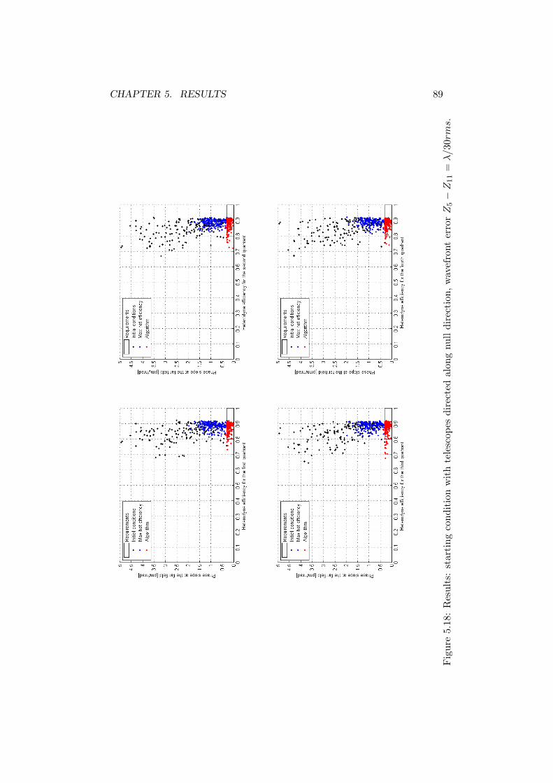
CHAPTER 5. RESULTS 89
Fig
ure
5.18
:R
esul
ts:
star
ting
cond
itio
nw
ith
tele
scop
esdi
rect
edal
ong
null
dire
ctio
n,w
avef
ront
erro
rZ
5−
Z11
=λ/30
rms.

CHAPTER 5. RESULTS 90
Figure 5.19: Frequency of heterodyne efficiency values (all quadrants con-sidered) for all the Zernike distributions tested. Initial condition: telescopesdirected along the null direction.
CHAPTER 5. RESULTS 91
Figure 5.20: Frequency of piston gradient values for all the Zernike distribu-tions tested. Initial condition: telescopes directed along the null direction.

CHAPTER 5. RESULTS 92
Zer
nike
dist
ribu
tion
µhe
tero
dyne
effici
ency
µpi
ston
grad
ient
σhe
tero
dyne
effici
ency
σpi
ston
grad
ient
(%)
(pm
/nra
d)
(%)
(pm
/nra
d)
wfe R
MS
=λ/10
0.69
151.
3968
0.10
371.
9527
wfe R
MS
=λ/15
0.80
410.
3422
0.06
110.
4070
wfe R
MS
=λ/17
0.82
710.
3092
0.05
180.
3088
wfe R
MS
=λ/20
0.85
120.
2572
0.04
050.
2364
wfe R
MS
=λ/22
0.85
930.
2487
0.03
650.
1880
wfe R
MS
=λ/25
0.86
670.
2308
0.03
490.
1892
wfe R
MS
=λ/27
0.87
270.
2019
0.03
500.
1024
wfe R
MS
=λ/30
0.87
450.
2159
0.03
600.
0713
Tab
le5.
2:M
ean
valu
eµ
and
stan
dard
devi
atio
nσ
ofhe
tero
dyne
effici
ency
and
pist
ongr
adie
ntre
sult
edw
hen
asst
arti
ngco
ndit
ion
the
tele
scop
esar
edi
rect
edal
ong
thei
rnu
lldi
rect
ion.

CHAPTER 5. RESULTS 93
wavefront error only in a few cases reaches values near to the boundaries(wfeZ4 = ±0.05) The cases out of the requirements instead coincide withthe points with large in-plane angles and out-of-plane angles. With largepointing angles, both the heterodyne efficiency and the piston gradient, ascan seen in the figure, present some cases that do not reach the values re-quested. This does not happen at the same time for the same telescopecouple: usually, only one of the quantities of interest (either efficiency orpiston gradient)is out of the requirements for these large angles.
As previously explained, the number of measurements used to reach thefinal solution is also important. In Fig.5.25 and 5.24 the function evaluationsused for each case of each Zernike distribution considered in the testingphase are reported. The difference between the initial conditions are againnegligible: the initial pointing angles do not influence the results of thealgorithm.
In both cases, the number of evaluations decreases with the reductionof the wavefront error at the pupil, but the effect is not so significant afterλ/22rms and for the smallest wavefront error, the measurements needed arestill too many for the calibration time.
In order to reduce the number of function evaluations necessary, an al-ternative approach has been found and described in Chapter 6. With thisdifferent procedure an arbitrary complex algorithm for finding the optimumsetting for PAAM, refocus and pointing can be implemented.

CHAPTER 5. RESULTS 94
Fig
ure
5.21
:Fin
alre
sult
sof
Mon
teca
rlo
Sim
ulat
ion
1000
case
sw
ith
wav
efro
nter
ror
ofλ/20
rms.
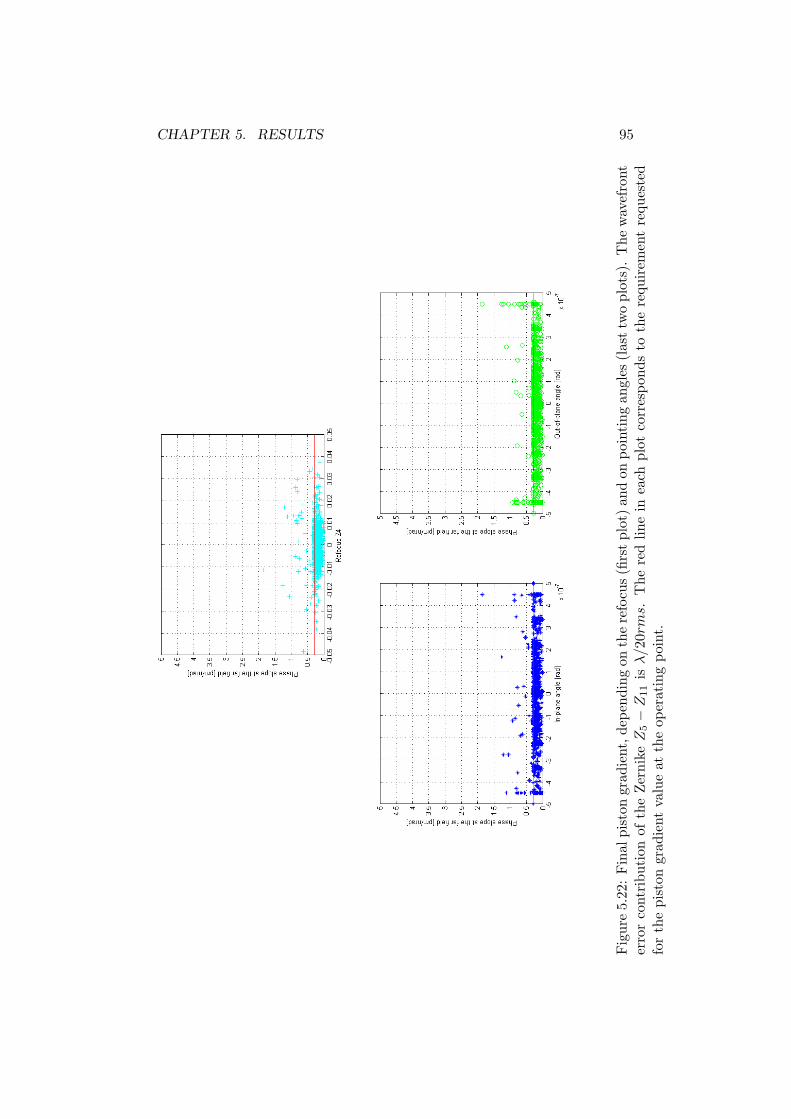
CHAPTER 5. RESULTS 95
Fig
ure
5.22
:Fin
alpi
ston
grad
ient
,dep
endi
ngon
the
refo
cus(fi
rstpl
ot)an
don
poin
ting
angl
es(l
asttw
opl
ots)
.T
hew
avef
ront
erro
rco
ntri
buti
onof
the
Zer
nike
Z5−
Z11
isλ/20
rms.
The
red
line
inea
chpl
otco
rres
pond
sto
the
requ
irem
ent
requ
este
dfo
rth
epi
ston
grad
ient
valu
eat
the
oper
atin
gpo
int.
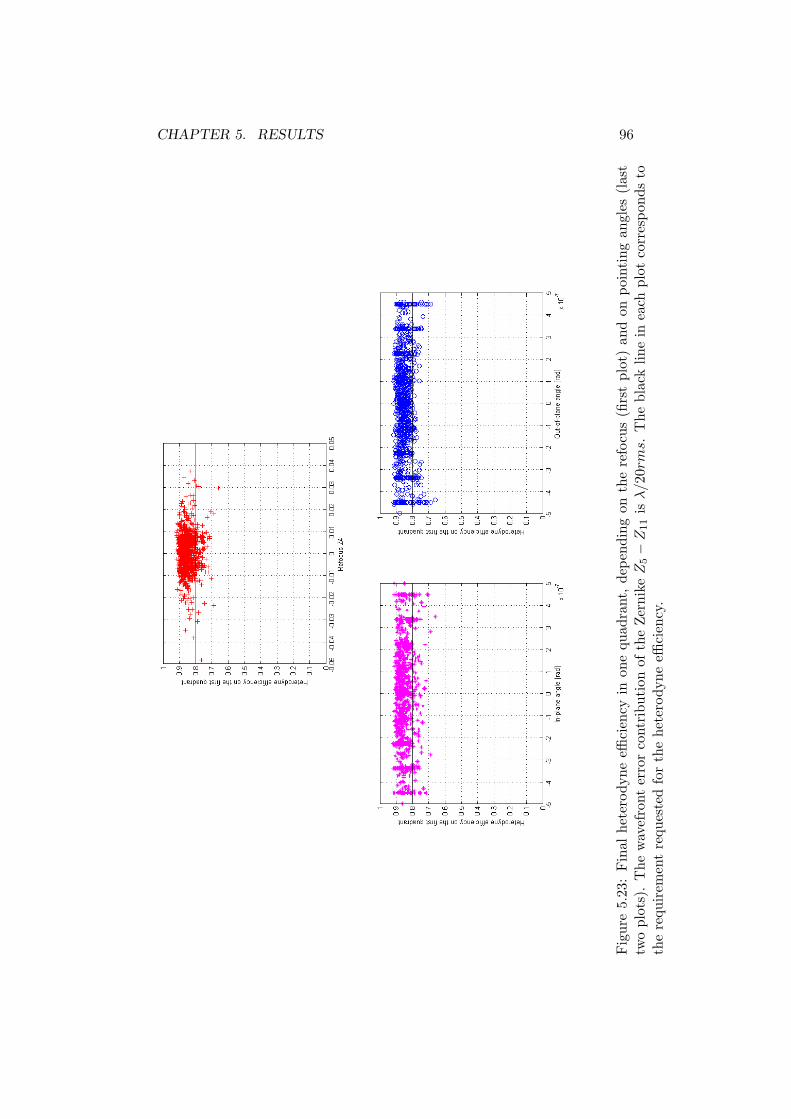
CHAPTER 5. RESULTS 96
Fig
ure
5.23
:Fin
alhe
tero
dyne
effici
ency
inon
equ
adra
nt,de
pend
ing
onth
ere
focu
s(fi
rst
plot
)an
don
poin
ting
angl
es(l
ast
two
plot
s).
The
wav
efro
nter
ror
cont
ribu
tion
ofth
eZer
nike
Z5−
Z11
isλ/20
rms.
The
blac
klin
ein
each
plot
corr
espo
nds
toth
ere
quir
emen
tre
ques
ted
for
the
hete
rody
neeffi
cien
cy.

CHAPTER 5. RESULTS 97
Figure 5.24: Function evaluations needed in the algorithm, starting withtwo telescopes facing along the geometrical line connecting the respectivetest masses.

CHAPTER 5. RESULTS 98
Figure 5.25: Function evaluations needed in the algorithm, starting withtwo telescopes facing along the null direction in the sense of DWS.

Chapter 6
Inverse Problem
6.1 Assumptions and Goals
Another way to face the problem of finding the best configuration of thetwo telescopes in one arm of the interferometer, is to estimate the Zernikedistribution of the telescope from the measurements at the far field in somepoints. In this way, it should be possible to rebuild an approximated far fieldand then find the better configuration of the telescope using the estimationmodel.
The basic idea is to minimize the error between the approximated fieldand the real one, changing some or all Zernike terms. Once the approximatedfield has been defined, the model and the algorithm described previously findthe best configuration with very few additional measurements of the field.
The function to minimize is defined as:
ε :=
√√√√∑i
[(∂pfferr(φyi , φzi , Z5, .., .Z11)
∂y
)2
+(
∂pfferr(φyi , φzi , Z5, .., .Z11)∂z
)2]
(6.1)where
pfferr(φyi , φzi , Z5, .., .Z11) = pffreal(φyi , φzi)− pffapprox(φyi , φzi , Z5, ..., Z11)
In this way it is possible to consider the components of the piston gra-dient in the two directions and to have a better estimation of the absolutevalue.
In order to see which Zernike polynomials give the most significant con-
99

CHAPTER 6. INVERSE PROBLEM 100
tribute on the far field piston and piston gradient, a starting analysis on thefirst 22 terms has been done. For each Zernike term the same wavefronterror contribution has been considered, in order to have an objective esti-mation of the different effect. In the next figures (Figg.6.1-6.2-6.3) the effecton the phase at the exit pupil, on the piston and the piston gradient at thefar field of each singular Zernike polynomial, from Z4 to Z22, is illustrated.
As can be seen in Fig.6.1, at the exit pupil each polynomial gives moreor less the same contribution to the phase distribution, as expected (in fact,the wavefront error contribution is the same for each term of the Zernikedistribution).
After free-space propagation, the effects of each polynomials are differ-ent, in terms of shape and order of magnitude. The plots in Fig.6.2 representthe piston at the far field, around the operating point, for each Zernike poly-nomial.
The far field generated by Z4-Z5-Z6-Z11-Z12-Z13 is two order of mag-nitude bigger than the field generated by Z7-Z8-Z9-Z10 and by the higherorder terms. The terms associated with Z4-Z11-Z22 give all the same effectat the far field, as the terms Z5-Z13 and Z6-Z12 respectively. An additionalproof of these effects on the far field is given by the plots of the pistongradient, in Fig.6.3.
Also in these plots is clear that some Zernike polynomials give moresignificant contributions than other ones. For this reason, it is possible toapproximate the field for the next analysis using only these few terms andnot the all 22 Zernike polynomials. In the next analysis, two approachesare faced. First of all, the evaluation of Z4 is not taken in account in thiscontext: its contribution can be changed with the refocus mechanism andso it is considered now already known. A first approximation of the fieldis computed estimating all the first eleven terms (from Z5): in this casethe relevant effects of Z12-Z13 are included in the study of Z5-Z6, as inthe far field they contribute with the same piston shape. This study iscritical because it is really slow. For this reason, a second strategy has beenimproved: an approximated far field is computed using a smaller number ofZernike polynomials which give a most significant contribution at the pistonand piston gradient around the operating point.
For the evaluation of the far field a measurement grid is necessary: thenumber of function evaluations needed has to be small but sufficient to
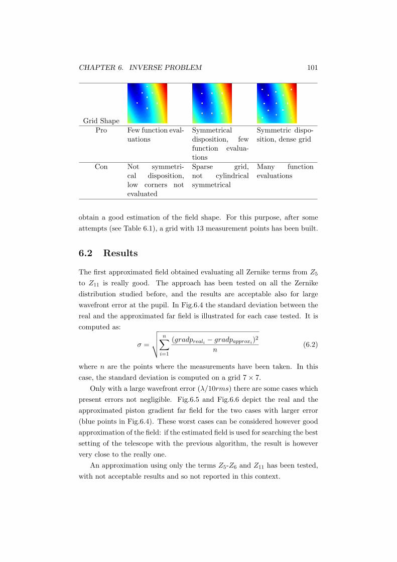
CHAPTER 6. INVERSE PROBLEM 101
Grid ShapePro Few function eval-
uationsSymmetricaldisposition, fewfunction evalua-tions
Symmetric dispo-sition, dense grid
Con Not symmetri-cal disposition,low corners notevaluated
Sparse grid,not cylindricalsymmetrical
Many functionevaluations
obtain a good estimation of the field shape. For this purpose, after someattempts (see Table 6.1), a grid with 13 measurement points has been built.
6.2 Results
The first approximated field obtained evaluating all Zernike terms from Z5
to Z11 is really good. The approach has been tested on all the Zernikedistribution studied before, and the results are acceptable also for largewavefront error at the pupil. In Fig.6.4 the standard deviation between thereal and the approximated far field is illustrated for each case tested. It iscomputed as:
σ =
√√√√ n∑i=1
(gradpreali − gradpapproxi)2
n(6.2)
where n are the points where the measurements have been taken. In thiscase, the standard deviation is computed on a grid 7× 7.
Only with a large wavefront error (λ/10rms) there are some cases whichpresent errors not negligible. Fig.6.5 and Fig.6.6 depict the real and theapproximated piston gradient far field for the two cases with larger error(blue points in Fig.6.4). These worst cases can be considered however goodapproximation of the field: if the estimated field is used for searching the bestsetting of the telescope with the previous algorithm, the result is howeververy close to the really one.
An approximation using only the terms Z5-Z6 and Z11 has been tested,with not acceptable results and so not reported in this context.

CHAPTER 6. INVERSE PROBLEM 102
The second approach uses Zernike terms: Z5-Z6-Z7-Z8 and Z11. Theother ones, in the approximated field, are set to zero. This procedure isfaster than the previous one and the results, in terms of error as explainedabove, are depicted in Fig.6.7.
In this second approximation the errors are sensitivity larger. For largewavefront error (λ/10rms) two cases are illustrated in Fig.6.8 and 6.9. Inthe first one, the approximated field is not acceptable: the field shape isstill similar but the scale is completely wrong. This is probably due to theimportance of the terms Z9 and Z10, not considered in the approximation.In the second case, even if the error computed is high (σ = 1.4679) the twofields are comparable and the studied algorithm ran on the approximatedfield would still give good results.
Going toward Zernike distribution with smaller wavefront error at thepupil, the results become sensitivity better. Already with a wavefront errorof λ/15rms, the higher standard deviation found between real and approxi-mated field is σ = 0.7122. The respective fields are shown in Fig.6.10. Fromthese results it is clear that, for this different approach at the problem, alsoan evaluation of the only Z5-Z6-Z7-Z8 and Z11 is sufficient for an acceptableapproximation of the far field piston gradient, starting from a wavefronterror at the pupil of at maximum λ/15rms.
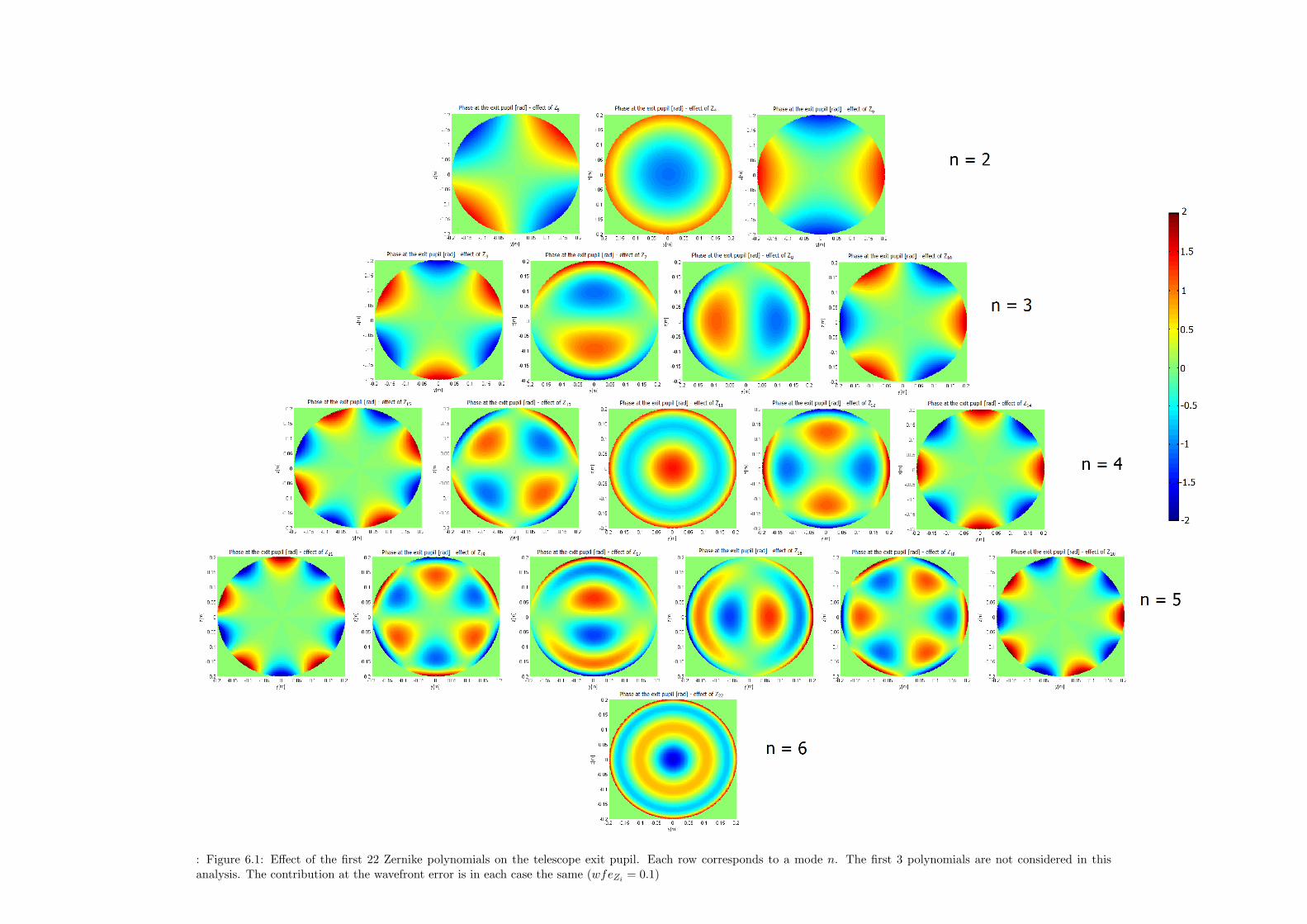
: Figure 6.1: Effect of the first 22 Zernike polynomials on the telescope exit pupil. Each row corresponds to a mode n. The first 3 polynomials are not considered in thisanalysis. The contribution at the wavefront error is in each case the same (wfeZi = 0.1)

: Figure 6.2: Effect of the first 22 Zernike polynomials on the far field piston. Each row corresponds to a mode n. The first 3 polynomials are not considered in this analysis.Thecontribute at the wavefront error is in each case the same (wfeZi = 0.1)
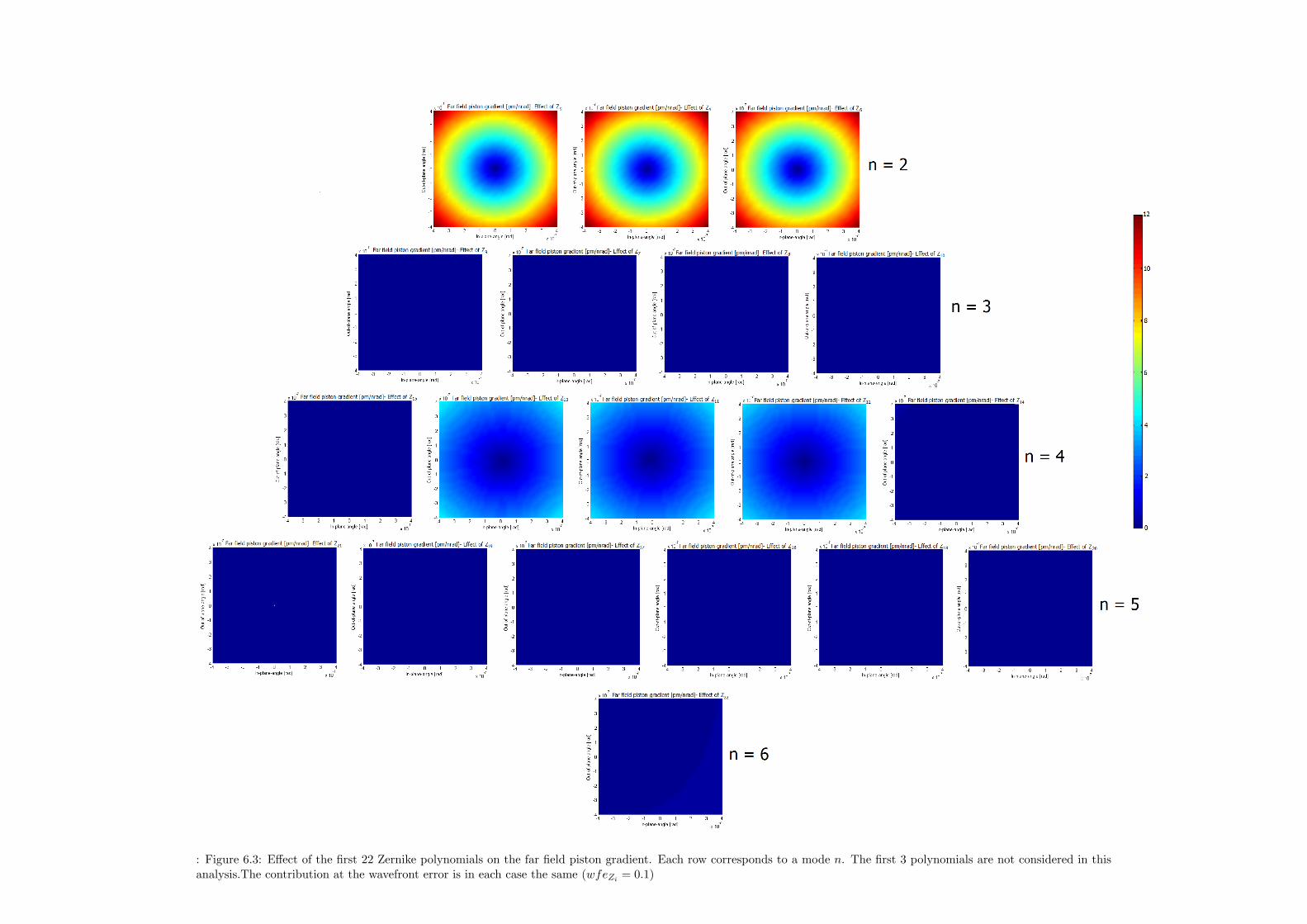
: Figure 6.3: Effect of the first 22 Zernike polynomials on the far field piston gradient. Each row corresponds to a mode n. The first 3 polynomials are not considered in thisanalysis.The contribution at the wavefront error is in each case the same (wfeZi = 0.1)

CHAPTER 6. INVERSE PROBLEM 106
Figure 6.4: Error between real and approximated far field piston gradient,for different Zernike distributions. Evaluation of all terms from Z5 to Z11.Blue points correspond to the largest error found.

CHAPTER 6. INVERSE PROBLEM 107
Figure 6.5: Real (left) and approximated (right) piston gradient for σ =0.4203. Wavefront error at the pupil λ/10rms. Approximation of all Zerniketerms.
Figure 6.6: Real (left) and approximated (right) piston gradient for σ =0.0567. Wavefront error at the pupil λ/10rms. Approximation of all Zerniketerms.
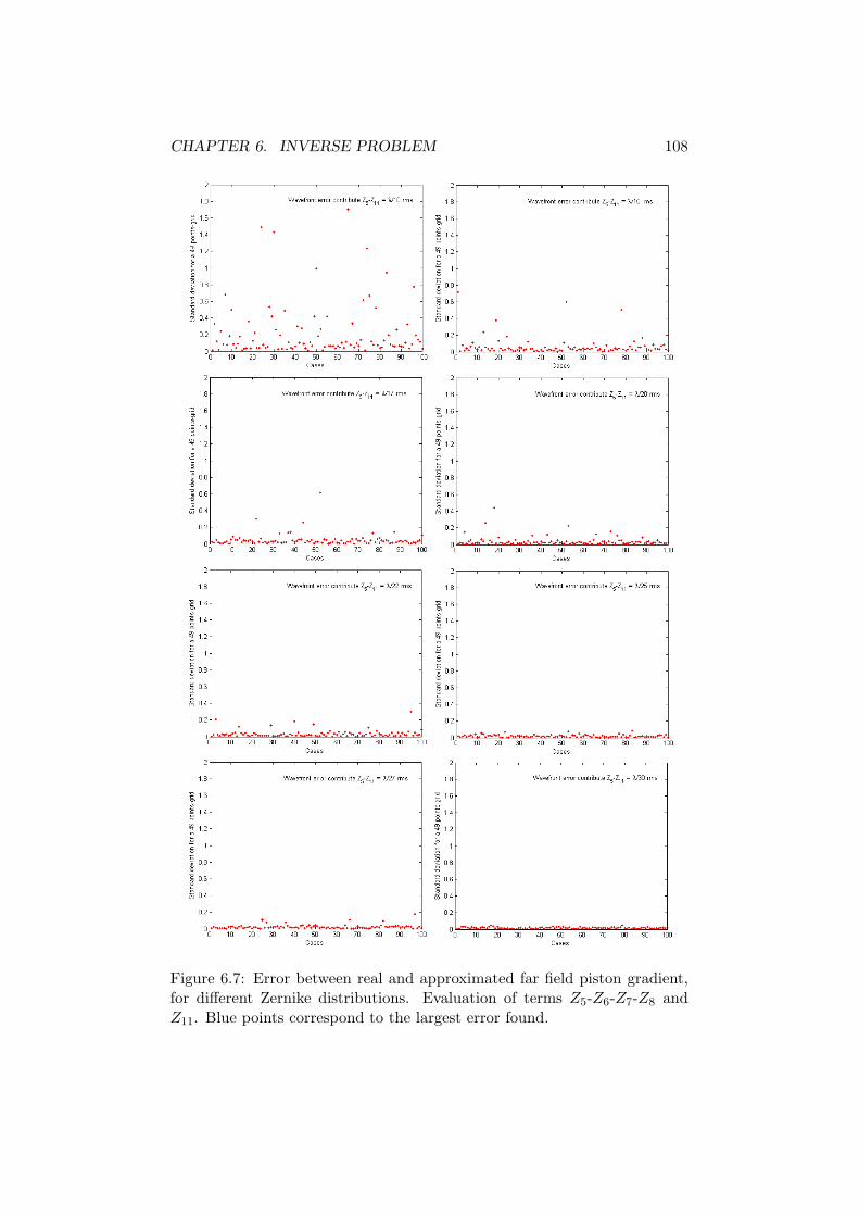
CHAPTER 6. INVERSE PROBLEM 108
Figure 6.7: Error between real and approximated far field piston gradient,for different Zernike distributions. Evaluation of terms Z5-Z6-Z7-Z8 andZ11. Blue points correspond to the largest error found.

CHAPTER 6. INVERSE PROBLEM 109
Figure 6.8: Real (left) and approximated (right) piston gradient for σ =1.7562. Wavefront error at the pupil λ/10rms. Approximation of Zerniketerms:Z5-Z6-Z7-Z8-Z11.
Figure 6.9: Real (left) and approximated (right) piston gradient for σ =1.5172. Wavefront error at the pupil λ/10rms.Approximation of Zerniketerms:Z5-Z6-Z7-Z8-Z11.
Figure 6.10: Real (left) and approximated (right) piston gradient for σ =0.7122. Wavefront error at the pupil λ/15rms.Approximation of Zerniketerms:Z5-Z6-Z7-Z8-Z11.
Chapter 7
Conclusion and Outlook on
future work
The results of the algorithm show that also with a small wavefront errorat the pupil, there are still some cases that cannot reach the requirements.The problem with small wavefront error is to keep the heterodyne efficiencywithin an acceptable value, while the piston gradient in these cases is almostalways in the requirements. For a wavefront error of λ/30rms the 1% of casescannot reach an acceptable piston gradient value at the operating point,while more or less the 10% do not have enough heterodyne efficiency on oneof the four quadrants. The reason is also that four values are computedfor the heterodyne efficiency and usually only in one or two quadrants theefficiency is too small. In all these cases, however, the heterodyne efficiencyis not so small, because it is always over 70%.
Probably this difference between the two quantities is also due to theparticularly strategy adopted: the efficiency is maximized at the first stepof the algorithm, and then its value is not more controlled. With a differentstrategy it should be possible to obtain higher values of this quantity.
The introduction of a two dimensional PAAM can be helpful at thispurpose. As seen, the PAAM does not effect the received beam (and sothe heterodyne efficiency) but can move the far field and changes the pistongradient at the operating point. The problem in this additional evaluationis the number of additional measurements needed. A deeper study in thissense is suggested.
The same cases analyzed with the algorithm have been tested with the
110
CHAPTER 7. CONCLUSION AND OUTLOOK ON FUTURE WORK111
ideal optimization described in Chapter 3. The cases out of the requirementsnot always correspond for the both optimizations. If the wavefront error islarge the cases that do not reach acceptable values are more or less thesame for the two routines. These are probably pathological cases, for whichit is not possible to find an acceptable configuration. If the wavefront errorbecomes smaller the cases out of requirements decrease and start to deviate.This means that it should be in theory possible to find the best configurationfor almost all the cases with these Zernike distributions. Note that theideal optimization uses a one-dimensional PAAM and not finite functionevaluations.
The number of function evaluations is the critical result of the imple-mented algorithm. The number of measurements necessary does not de-crease so sensitivity with smaller wavefront error at the pupil. The approxi-mation of the two dimensional field for the line search method still requiresa certain number of measurements.
It has to note that in the present model all the measurements taken atthe far field during the calibration procedure have been used only once inthe algorithm. They can in theory be used also in the subsequent steps,for a better approximation of the field. This procedure would reduce thenumber of the function evaluations needed.
The inverse approach seems to be a good alternative at the problem ofthe large number of measurements necessary. A grid with 13 evaluationpoints corresponds to about three days of calibration procedure, but theapproximated field obtained is quite good also with large wavefront error atthe pupil (with an error of λ/15rms the approximation is already accept-able). On the approximated field an arbitrary complex algorithm can beapplied and this is surely an advantage. Future studies must confirm thisresult to be working also in the presence of measurement noise.

Bibliography
[1] LISA: Laser Interferometer Space Antenna. http://lisa.nasa.gov. Citedon 01 December 2009.
[2] ESA Science and Technology:LISA. http://sci.esa.int/science-e/www/area/index.cfm?fareaid=27. Cited on 01 December 2009.
[3] Peter Gath. LISA-ASD-DD-5001, Mission Design Description. EADSAstrium, 2008.
[4] Marcel Berger. LISA-ASD-DD-3001, Payload Preliminary Design De-scription. EADS Astrium, 2008.
[5] Dennis Weise and Pierangelo Marenaci. PM1, Technical Overview.EADS Astrium, 2009.
[6] Peter Gath and LISA Mission Formulation Team. Workshop on Satel-lite Dynamics: Modelling In-Orbit Calibration and Data Processing.EADS Astrium, 2008.
[7] Marc Hirth. Alignment Performance Model for LISA. University ofStuttgart, Insitute of Flight Mechanics and Control, 2009.
[8] Robert J. Noll. Zernike polynomials and atmospheric turbolence. Jour-nal of Optical society of America, 66, 1976.
[9] Dennis Weise Astrium GmbH Satellites. Far Field Propagator for Ar-bitrary Input Wavefront. 2009.
[10] Bahaa E. A. Saleh and Malvin Carl Teich. Fundamentals of Photonics.Wiley Interscience, 2007.
112

BIBLIOGRAPHY 113
[11] William H. Press, Saul A. Teukolsky, William T. Vetterling, andBrian P. Flannery. Numerical Recipes in C - The Art of ScientificComputing. Cambrige University Press.
[12] John T. Betts. Practical Methods for Optimal Control Using Non-Linear Programming. SIAM DC03.