Universita degli Studi di Roma “La Sapienza”Dipartimento di Informatica e Sistemistica “A. Ruberti”

Gianni Di Pillo and Laura Palagi

Nonlinear Programming: Introduction,Unconstrained and Constrained Optimization

Tech. Rep. 25-01

Dipartimento di Informatica e Sistemistica “A. Ruberti”, Universita di Roma “La Sapienza”via Buonarroti 12 - 00185 Roma, Italy.E-mail: dipillo@dis.uniroma1.it, palagi@dis.uniroma1.it.

Nonlinear Programming: Introduction, Unconstrained and

Constrained Optimization

Gianni Di Pillo and Laura Palagi

Contents

1 Introduction 11.1 Problem Definition . . . . . . . . . . . . . . . . . . . . . . . . . . . . . . . . . . . 11.2 Optimality Conditions . . . . . . . . . . . . . . . . . . . . . . . . . . . . . . . . . 21.3 Performance of Algorithms . . . . . . . . . . . . . . . . . . . . . . . . . . . . . . 4

1.3.1 Convergence and Rate of Convergence . . . . . . . . . . . . . . . . . . . . 41.3.2 Numerical Behaviour . . . . . . . . . . . . . . . . . . . . . . . . . . . . . . 5

1.4 Selected Bibliography . . . . . . . . . . . . . . . . . . . . . . . . . . . . . . . . . 5

2 Unconstrained Optimization 62.1 Line Search Algorithms . . . . . . . . . . . . . . . . . . . . . . . . . . . . . . . . 72.2 Gradient Methods . . . . . . . . . . . . . . . . . . . . . . . . . . . . . . . . . . . 92.3 Conjugate Gradient Methods . . . . . . . . . . . . . . . . . . . . . . . . . . . . . 92.4 Newton’s Methods . . . . . . . . . . . . . . . . . . . . . . . . . . . . . . . . . . . 12

2.4.1 Line Search Modifications of Newton’s Method . . . . . . . . . . . . . . . 122.4.2 Trust Region Modifications of Newton’s Method . . . . . . . . . . . . . . 142.4.3 Truncated Newton’s Methods . . . . . . . . . . . . . . . . . . . . . . . . . 16

2.5 Quasi-Newton Methods . . . . . . . . . . . . . . . . . . . . . . . . . . . . . . . . 172.6 Derivative Free Methods . . . . . . . . . . . . . . . . . . . . . . . . . . . . . . . . 192.7 Selected Bibliography . . . . . . . . . . . . . . . . . . . . . . . . . . . . . . . . . 21

3 Constrained Optimization 213.1 Introduction . . . . . . . . . . . . . . . . . . . . . . . . . . . . . . . . . . . . . . . 213.2 Unconstrained Sequential Methods . . . . . . . . . . . . . . . . . . . . . . . . . . 22

3.2.1 The Quadratic Penalty Method . . . . . . . . . . . . . . . . . . . . . . . . 223.2.2 The Logarithmic Barrier Method . . . . . . . . . . . . . . . . . . . . . . . 233.2.3 The Augmented Lagrangian Method . . . . . . . . . . . . . . . . . . . . . 25

3.3 Unconstrained Exact Penalty Methods . . . . . . . . . . . . . . . . . . . . . . . . 273.4 Sequential Quadratic Programming Methods . . . . . . . . . . . . . . . . . . . . 28

3.4.1 The Line Search Approach . . . . . . . . . . . . . . . . . . . . . . . . . . 323.4.2 The Trust Region Approach . . . . . . . . . . . . . . . . . . . . . . . . . . 32

3.5 Feasible Direction Methods . . . . . . . . . . . . . . . . . . . . . . . . . . . . . . 333.6 Selected Bibliography . . . . . . . . . . . . . . . . . . . . . . . . . . . . . . . . . 35

1 Introduction

Nonlinear Programming (NLP) is the broad area of applied mathematics that addresses opti-mization problems when nonlinearity in the functions are envolved. In this chapter we introducethe problem, and making reference to the smooth case, we review the standard optimality con-ditions that are at the basis of most algorithms for its solution. Then, we give basic notionsconcerning the performance of algorithms, in terms of convergence, rate of convergence, andnumerical behaviour.

1.1 Problem Definition

We consider the problem of determining the value of a vector of decision variables x ∈ IRn thatminimizes an objective function f : IRn → IR, when x is required to belong to a feasible setF ⊆ IRn; that is we consider the problem:

minx∈F

f(x). (1)

Two cases are of main interest:- the feasible set F is IRn, so that Problem (1) becomes:

minx∈IRn

f(x); (2)

in this case we say that Problem (1) is unconstrained. More in general, Problem (1) is uncon-strained if F is an open set. The optimality conditions for unconstrained problems stated in§1.2 hold also in the general case. Here for simplicity we assume that F = IRn.- the feasible set is described by inequality and/or equality constraints on the decision variables:

F = x ∈ IRn : gi(x) ≤ 0, i = 1, . . . , p; hj(x) = 0, j = 1, . . . ,m;

then Problem (1) becomes:minx∈IRn

f(x)

g(x) ≤ 0h(x) = 0,

(3)

with h : IRn → IRm and g : IRn → IRp. In this case we say that Problem (1) is constrained.Problem (1) is a Nonlinear Programming (NLP) problem when at least one, among the

problem functions f , gi, i = 1, . . . , p, hj , j = 1, . . . ,m, is nonlinear in its argument x.Usually it is assumed that in Problem (3) the number m of equality constraints is not larger

than the number n of decision variables. Otherwise the feasible set could be empty, unless thereis some dependency among the constraints. If only equality (inequality) constraints are present,Problem (3) is called an equality (inequality) constrained NLP problem.

In the following we assume that the problem functions f, g, h are at least continuouslydifferentiable in IRn.

When f is a convex function and F is a convex set, Problem (1) is a convex NLP problem.In particular, F is convex if the equality constraint functions hj are affine and the inequalityconstraint functions gi are convex. Convexity adds a lot of structure to the NLP problem, andcan be exploited widely both from the theoretical and the computational point of view. If f isconvex quadratic and h, g are affine, we have a Quadratic Programming problem. This is a caseof special interest. Here we will confine ourselves to general NLP problems, without convexityassumptions.

A point x∗ ∈ F is a global solution of Problem (1) if f(x∗) ≤ f(x), for all x ∈ F ; it isa strict global solution if f(x∗) < f(x), for all x ∈ F , x = x∗. A main existence result for a

1

constrained problem is that a global solution exists if F is compact (Weierstrass Theorem).An easy consequence for unconstrained problems is that a global solution exists if the level setLα = x ∈ IRn : f(x) ≤ α is compact for some finite α.

A point x∗ ∈ F is a local solution of Problem (1) if there exists an open neighborhood Bx∗of x∗ such that f(x∗) ≤ f(x), for all x ∈ F ∩ Bx∗ ; it is a strict local solution if f(x∗) < f(x),for all x ∈ F ∩ Bx∗ , x = x∗. Of course, a global solution is also a local solution.

To determine a global solution of a NLP problem is in general a very difficult task. Usu-ally, NLP algorithms are able to determine only local solutions. Nevertheless, in practicalapplications, also to get a local solution can be of great worth.

We introduce some notation. We denote by the apex , the transpose of a vector or amatrix. Given a function v : IRn → IR, we denote by ∇v(x) the gradient vector and by ∇2v(x)the Hessian matrix of v. Given a vector function w : IRn → IRq, we denote by ∇w(x) then × q matrix whose columns are ∇wj(x), j = 1, . . . , q. Given a vector y ∈ IRq we denote byy its Euclidean norm. Let K ⊂ 1, . . . , q be an index subset, y be a vector with componentsyi, i = 1, . . . , q, and A be a matrix with columns aj , j = 1, . . . , q. We denote by yK the subvector of y with components yi such that i ∈ K and by AK the submatrix of A made up of thecolumns aj with j ∈ K.

1.2 Optimality Conditions

Local solutions must satisfy necessary optimality conditions (NOC).For the unconstrained Problem (2) we have the well know result of classical calculus:

Proposition 1.1 Let x∗ be a local solution of Problem (2), then

∇f(x∗) = 0; (4)

moreover, if f is twice continuously differentiable, then

y ∇2f(x∗)y ≥ 0, ∀y ∈ IRn. (5)

For the constrained problem (3), most of the NOC commonly used in the development ofalgorithms assume that at a local solution the constraints satisfy some qualification conditionto prevent the occurrence of degenerate cases. These conditions are usually called constraintsqualifications and among them the linear independence constraints qualification (LICQ) is thesimplest and by far the most invoked.

Let x ∈ F . We say that the inequality constraint gi is active at x if gi(x) = 0. We denoteby Ia(x) the index set of inequality constraints active at x:

Ia(x) = i ∈ 1, . . . , p : gi(x) = 0. (6)

Of course, any equality constraint hj , is active at x. LICQ is satisfied at x if the gradients ofthe active constraints ∇gIa(x), ∇h(x), are linearly independent.

Under LICQ, the NOC for Problem (3) are stated making use of the (generalized) La-grangian function:

L(x,λ, µ) = f(x) + λ g(x) + µ h(x), (7)

where λ ∈ IRp, µ ∈ IRm are called (generalized Lagrange) multipliers, or dual variables.The so called Karush-Kuhn-Tucker (KKT) NOC are stated as follows:

Proposition 1.2 Assume that x∗ is a local solution of Problem (3) and that LICQ holds atx∗; then multipliers λ∗ ≥ 0, µ∗ exist such that:

∇xL(x∗,λ∗, µ∗) = 0, (8)

λ∗ g(x∗) = 0;

2

moreover, if f, g, h are twice continuously differentiable, then:

y ∇2xL(x∗,λ∗, µ∗)y ≥ 0, ∀y ∈ N (x∗),

where:N (x∗) = y ∈ IRn : ∇gIa(x∗) y = 0;∇h(x∗) y = 0.

A point x∗ satisfying the NOC conditions (8) together with some multipliers λ∗, µ∗ is calleda KKT point.

If a point x∗ ∈ F satisfies a sufficient optimality condition, then it is a local solution ofProblem (1). For general NLP problems, sufficient optimality conditions can be stated underthe assumption that the problem functions are twice continuously differentiable, so that wehave second order sufficiency conditions (SOSC).

For the unconstrained Problem (2) we have the SOSC:

Proposition 1.3 Assume that x∗ satisfies the NOC of Proposition (1.1). Assume further that

y ∇2f(x∗)y > 0, ∀y ∈ IRn, y = 0,

that is that assume that ∇2f(x∗) is positive definite. Then x∗ is a strict local solution of Problem(2).

For the constrained Problem (3) we have the SOSC:

Proposition 1.4 Assume that x∗ ∈ F and λ∗, µ∗ satisfy the NOC of Proposition (1.2). As-sume further that

y ∇2xL(x∗,λ∗, µ∗)y > 0, ∀y ∈ P(x∗), y = 0, (9)

where:P(x∗) = y ∈ IRn : ∇gIa(x∗) y ≤ 0, ∇h(x∗) y = 0;

∇gi(x∗) y = 0, i ∈ Ia(x∗) with λ∗i > 0;then x∗ is a strict local solution of Problem (3).

Note that P(x∗) is a polyhedral set, while N (x∗) is the null space of a linear operator,with N (x∗) ⊆ P(x∗). However, if λ∗i > 0 for all i ∈ Ia(x∗), then N (x∗) = P(x∗). Whenthis happens, we say that the strict complementarity assumption is satisfied by g(x∗) and λ∗.Strict complementarity is a very favorable circumstance, because it is much simpler to deal withthe null space of a linear operator than with a general polyhedron. In particular, there existsa simple algebraic criterion to test whether the quadratic form y ∇2xL(x∗,λ∗, µ∗)y is positivedefinite on N (x∗).

Note also that, if in Proposition 1.4 we substitute the set P(x∗) with the set

N+(x∗) = y ∈ IRn : ∇h(x∗) y = 0, ∇gi(x∗) y = 0, i ∈ Ia(x∗) with λ∗i > 0,

we still have a sufficient condition, since P(x∗) ⊆ N+(x∗), and again N+(x∗) is the null spaceof a linear operator. However the condition obtained is stronger then the original one, andindeed it is known as the strong second order sufficient condition (SSOSC).

Finally, we point out that, under the strict complementarity assumption, N (x∗) = P(x∗) =N+(x∗), so that all the SOSC for Problem (3) considered above reduce to the same condition.

A main feature of convex problems is that a (strict) local solution is also a (strict) globalsolution. Moreover, when f is (strictly) convex and, if present, gi are convex and hj are affine,the NOC given in terms of first order derivatives are also sufficient for a point x∗ to be a (strict)global solution.

3

Optimality conditions are fundamental in the solution of NLP problems. If it is knownthat a global solution exists, the most straightforward method to employ them is as follows:find all points satisfying the first order necessary conditions, and declare as global solutionthe point with the smallest value of the objective function. If the problem functions are twicedifferentiable, we can also check the second order necessary condition, filtering out those pointsthat do not satisfy it; for the remaining candidates, we can check a second order sufficientcondition to find local minima.

It is important to realize, however, that except for very simple cases, using optimalityconditions as described above does not work. The reason is that, even for an unconstrainedproblem, to find a solution of the system of equations ∇f(x) = 0 is nontrivial; algorithmically,it is usually as difficult as solving the original minimization problem.

The principal context in which optimality conditions become useful is the developmentand analysis of algorithms. An algorithm for the solution of Problem (1) produces a sequencexk, k = 0, 1, . . . , of tentative solutions, and terminates when a stopping criterion is satisfied.Usually the stopping criterion is based on satisfaction of necessary optimality conditions withina prefixed tolerance; moreover, necessary optimality conditions often suggest how to improvethe current tentative solution xk in order to get the next one xk+1, closer to the optimalsolution. Thus, necessary optimality conditions provide the basis for the convergence analysisof algorithms. On the other hand, sufficient optimality conditions play a key role in the analysisof the rate of convergence.

1.3 Performance of Algorithms

1.3.1 Convergence and Rate of Convergence

Let Ω ⊂ F be the subset of points that satisfy the first order NOC for Problem (1). Froma theoretical point of view, an optimization algorithm stops when a point x∗ ∈ Ω is reached.From this point of view, the set Ω is called the target set. Convergence properties are statedwith reference to the target set Ω. In the unconstrained case, a possible target set is Ω = x ∈IRn : ∇f(x) = 0 whereas in the constrained case Ω may be the set of KKT points satisfying(8).

Let xk, k = 0, 1, . . . be the sequence of points produced by an algorithm. Then, thealgorithm is globally convergent if a limit point x∗ of xk exists such that x∗ ∈ Ω for anystarting point x0 ∈ IRn; it is locally convergent if the existence of the limit point x∗ ∈ Ω can beestablished only if the starting point x0 belongs to some neighborhood of Ω.

The notion of convergence stated before is the weakest that ensures that a point xk arbi-trarily close to Ω can be obtained for k large enough. In the unconstrained case this impliesthat

limk→∞

inf ∇f(xk) = 0.

Nevertheless, stronger convergence properties can often be established. For instance thatany subsequence of xk possess a limit point, and any limit point of xk belongs to Ω; forthe unconstrained case, this means that

limk→∞

∇f(xk) = 0.

The strongest convergence requirement is that the whole sequence xk converges to a pointx∗ ∈ Ω.

In order to define the rate of convergence of an algorithm, it is assumed for simplicitythat the algorithm produces a sequence xk converging to a point x∗ ∈ Ω. The most widelyemployed notion of rate of convergence is the Q-rate of convergence, that considers the quotient

4

between two successive iterates given by xk+1 − x∗ / xk − x∗ . Then we say that the rate ofconvergence is Q-linear if there is a constant r ∈ (0, 1) such that:

xk+1 − x∗xk − x∗ ≤ r, for all k sufficiently large;

we say that the rate of convergence is Q-superlinear if:

limk→∞

xk+1 − x∗xk − x∗ = 0;

and we say that the rate of convergence is Q-quadratic if:

xk+1 − x∗xk − x∗ 2

≤ R, for all k sufficiently large,

where R is a positive constant, not necessarily less than 1. More in general, the rate of conver-gence is of Q-order p if there exists a positive constant R such that:

xk+1 − x∗xk − x∗ p

≤ R, for all k sufficiently large;

however a Q-order larger than 2 is very seldom achieved. Algorithms of common use are eithersuperlinearly or quadratically convergent.

1.3.2 Numerical Behaviour

Besides the theoretical performance, an important aspect of a numerical algorithm is its practi-cal performance. Indeed fast convergence rate can be overcome by a great amount of algebraicoperations needed at each iteration. Different measures of the numerical performance exist,even if direct comparison of CPU time remains the best way of verifying the efficiency of agiven method on a specific problem. However, when the computational burden in term of alge-braic operations per iteration is comparable, possible measures of performance can be given interms of number of iterations, number of objective function/constraints evaluations and numberof its/their gradient evaluations.

Measures of performance are of main relevance for large scale NLP problems. The notionof large scale is machine dependent so that it could be difficult to state a priori when a problemis large. Usually, an unconstrained problem with n ≥ 1000 is considered large whereas aconstrained problems without particular structure is considered large when n ≥ 100 and p+m ≥100. A basic feature of an algorithm for large scale problems is a low storage overhead neededto make practicable its implementation, and a measure of performance is usually the numberof matrix-vector products required. The main difficulty in dealing with large scale problems isthat effective algorithms for small scale problems do not necessarily translate into efficient oneswhen applied to solve large problems.

1.4 Selected Bibliography

In this section we give a list of books and surveys of general references in NLP. Of course thelist is by far not exhaustive; it includes only texts widely employed and currently found.

Several textbooks on applied optimization devote chapters to NLP theory and practice.Among them, the books by Gill et al. (1981), Minoux (1983), Luenberger (1994), Fletcher(1987), Nash and Sofer (1996) Bonnans et al. (1997) and Nocedal and Wright (1999).

5

More specialized textbooks, strictly devoted to NLP, are the ones by Zangwill (1969), Avriel(1976), McCormick (1983), Evtushenko (1985), Bazaraa et al. (1993), Polak (1997), Bertsekas(1999). A collection of survey papers on algorithmic aspects of NLP is in Spedicato (1994).

A particular emphasis on the mathematical foundations of NLP is given in Hestenes (1975),Giannessi (1982), Polyak (1987), Peressini et al. (1988), Jahn (1994), Rapsack (1997). A classi-cal reference on optimality conditions and constraint qualifications is the book by Mangasarian(1969).

The theoretical analysis of algorithms for NLP is developed in Zangwill (1969), Orthegaand Rheinboldt (1970), Bazaraa et al. (1993), Luenberger (1994), Polak (1997). For practicalaspects in the implementation of algorithms we refer again to Gill et al. (1981).

The search for global optima is treated for instance in Torn and Zilinskas (1989), Horst andPardalos (1995), Pinter (1996).

This chapter does not mention multiobjective optimization. Multiobjective NLP problemsare considered for instance in Rustem (1998), Miettinen (1999).

2 Unconstrained Optimization

In this chapter we consider algorithms for solving the unconstrained Nonlinear Programmingproblem (2)

minx∈IRn

f(x),

where x ∈ IRn is the vector of decision variables and f : IRn → IR is the objective function.The algorithms described in this section can be easily adapted to solve the constrained Problemminx∈F f(x) when F is an open set, provided that a feasible point x0 ∈ F is available.

In the following we assume for simplicity that the problem function f is twice continuouslydifferentiable in IRn even if in many cases only once continuously differentiability is needed.

We also assume that the standard assumption ensuring the existence of a solution of Problem(2) holds, namely that:

Assumption 2.1 The level set L0 = x ∈ IRn : f(x) ≤ f(x0) is compact, for some x0 ∈ IRn.The algorithm models treated in this section generate a sequence xk, starting from x0,

by the following iterationxk+1 = xk + αkdk, (10)

where dk is a search direction and αk is a stepsize along dk.Methods differentiate in the way the direction and the stepsize are chosen. Of course

different choices of dk and αk yield different convergence properties. Roughly speaking, thesearch direction affects the local behaviour of an algorithm and its rate of convergence whereasglobal convergence is often tied to the choice of the stepsize αk. The following propositionstates a rather general convergence result (Orthega 1988).

Proposition 2.2 Let xk be the sequence generated by iteration (10). Assume that: (i) dk = 0if ∇f(xk) = 0; (ii) for all k we have f(xk+1) ≤ f(xk); (iii) we have

limk→∞

∇f(xk) dkdk

= 0; (11)

(iv) for all k with dk = 0 we have

|∇f(xk) dk|dk

≥ c ∇f(xk) , with c > 0.

Then, either k exists such that xk ∈ L0 and ∇f(xk) = 0, or an infinite sequence is producedsuch that:

6

(a) xk ∈ L0;(b) f(xk) converges;(c)

limk→∞

∇f(xk) = 0. (12)

Condition (c) of Proposition 2.2 corresponds to say that any subsequence of xk possessa limit point, and any limit point of xk belongs to Ω. However, weaker convergence resultscan be proved (see Section 1). In particular in some cases, only condition

limk→∞

inf ∇f(xk) = 0 (13)

holds.Many methods are classified according to the information they use regarding the smoothness

of the function. In particular we will briefly describe gradient methods, conjugate gradientmethods, Newton’s and truncated Newton’s methods, quasi-Newton methods and derivativefree methods.

Most methods determine αk by means of a line search technique. Hence we start with a shortreview of the most used techniques and more recent developments in line search algorithms.

2.1 Line Search Algorithms

Line Search Algorithms (LSA) determine the stepsize αk along the direction dk. The aim ofdifferent choices of αk is mainly to ensure that the algorithm defined by (10) results to beglobally convergent, possibly without deteriorating the rate of convergence. A first possibilityis to set αk = α∗ with

α∗ = argminαf(xk + αdk),

that is αk is the value that minimizes the function f along the direction dk. However, unlessthe function f has some special structure (being quadratic), an exact line search is usually quitecomputationally costly and its use may not be worthwhile. Hence approximate methods areused. In the cases when ∇f can be computed, we assume that the condition

∇f(xk) dk < 0, for all k (14)

holds, namely we assume that dk is a descent direction for f at xk.Among the simplest LSAs is Armijo’s method, reported in Algorithm 1.The choice of the initial step ∆k is tied to the direction dk used. By choosing ∆k as in

Step 1, it is possible to prove that Armijo’s LSA finds in a finite number of steps a value αk

such thatf(xk+1) < f(xk), (15)

and that condition (11) holds.Armijo’s LSA finds a stepsize αk that satisfies a condition of sufficient decrease of the

objective function and implicitly a condition of sufficient displacement from the current pointxk.

In many cases it can be necessary to impose stronger conditions on the stepsize αk. Inparticular Wolfe’s conditions are widely employed. In this case, Armijo’s condition

f(xk + αdk) ≤ f(xk) + γα∇f(xk) dk (16)

is coupled either with condition

∇f(xk + αkdk) dk ≥ β∇f(xk) dk, (17)

7

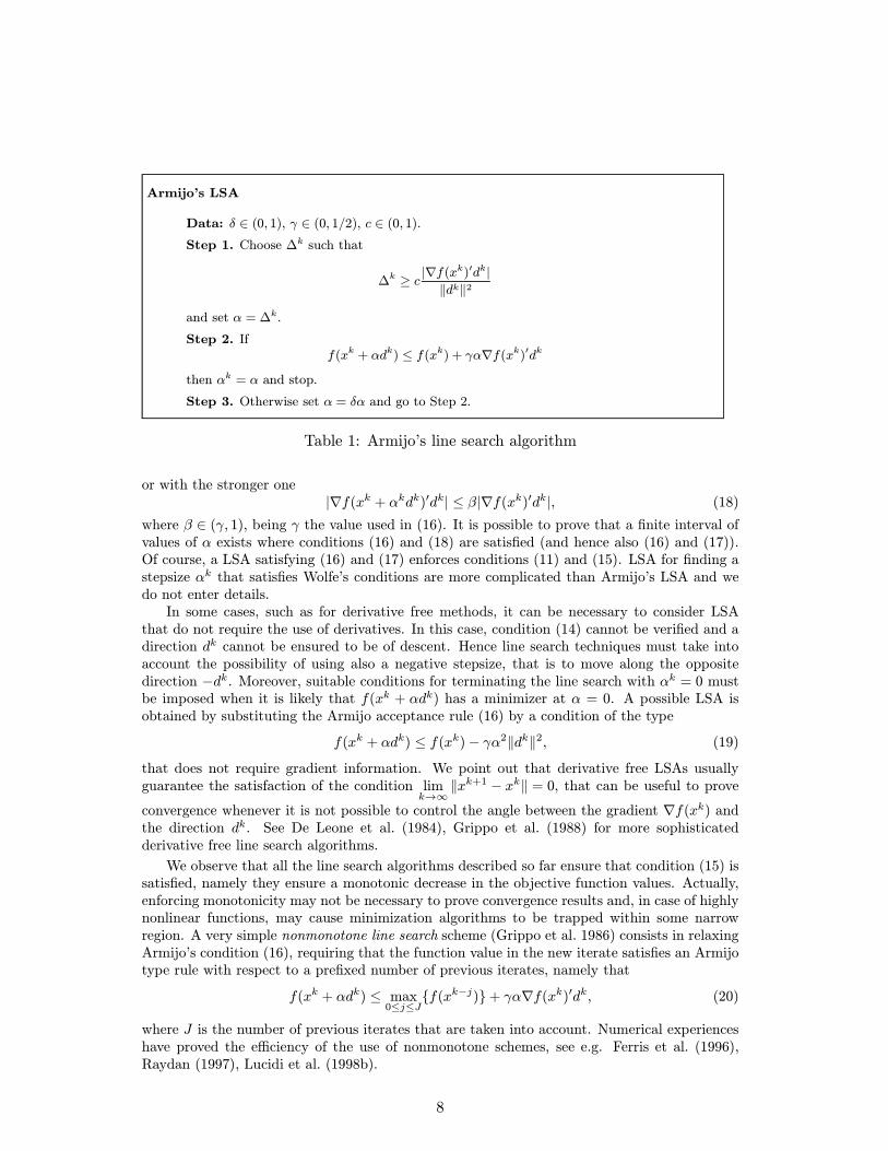
Armijo’s LSA

Data: δ ∈ (0, 1), γ ∈ (0, 1/2), c ∈ (0, 1).Step 1. Choose ∆k such that

∆k ≥ c |∇f(xk) dk|

dk 2

and set α = ∆k.

Step 2. Iff(xk + αdk) ≤ f(xk) + γα∇f(xk) dk

then αk = α and stop.

Step 3. Otherwise set α = δα and go to Step 2.

Table 1: Armijo’s line search algorithm

or with the stronger one|∇f(xk + αkdk) dk| ≤ β|∇f(xk) dk|, (18)

where β ∈ (γ, 1), being γ the value used in (16). It is possible to prove that a finite interval ofvalues of α exists where conditions (16) and (18) are satisfied (and hence also (16) and (17)).Of course, a LSA satisfying (16) and (17) enforces conditions (11) and (15). LSA for finding astepsize αk that satisfies Wolfe’s conditions are more complicated than Armijo’s LSA and wedo not enter details.

In some cases, such as for derivative free methods, it can be necessary to consider LSAthat do not require the use of derivatives. In this case, condition (14) cannot be verified and adirection dk cannot be ensured to be of descent. Hence line search techniques must take intoaccount the possibility of using also a negative stepsize, that is to move along the oppositedirection −dk. Moreover, suitable conditions for terminating the line search with αk = 0 mustbe imposed when it is likely that f(xk + αdk) has a minimizer at α = 0. A possible LSA isobtained by substituting the Armijo acceptance rule (16) by a condition of the type

f(xk + αdk) ≤ f(xk)− γα2 dk 2, (19)

that does not require gradient information. We point out that derivative free LSAs usuallyguarantee the satisfaction of the condition lim

k→∞xk+1 − xk = 0, that can be useful to prove

convergence whenever it is not possible to control the angle between the gradient ∇f(xk) andthe direction dk. See De Leone et al. (1984), Grippo et al. (1988) for more sophisticatedderivative free line search algorithms.

We observe that all the line search algorithms described so far ensure that condition (15) issatisfied, namely they ensure a monotonic decrease in the objective function values. Actually,enforcing monotonicity may not be necessary to prove convergence results and, in case of highlynonlinear functions, may cause minimization algorithms to be trapped within some narrowregion. A very simple nonmonotone line search scheme (Grippo et al. 1986) consists in relaxingArmijo’s condition (16), requiring that the function value in the new iterate satisfies an Armijotype rule with respect to a prefixed number of previous iterates, namely that

f(xk + αdk) ≤ max0≤j≤J

f(xk−j)+ γα∇f(xk) dk, (20)

where J is the number of previous iterates that are taken into account. Numerical experienceshave proved the efficiency of the use of nonmonotone schemes, see e.g. Ferris et al. (1996),Raydan (1997), Lucidi et al. (1998b).

8

2.2 Gradient Methods

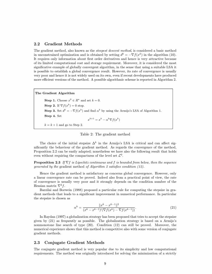
The gradient method, also known as the steepest descent method, is considered a basic methodin unconstrained optimization and is obtained by setting dk = −∇f(xk) in the algorithm (10).It requires only information about first order derivatives and hence is very attractive becauseof its limited computational cost and storage requirement. Moreover, it is considered the mostsignificative example of globally convergent algorithm, in the sense that using a suitable LSA itis possible to establish a global convergence result. However, its rate of convergence is usuallyvery poor and hence it is not widely used on its own, even if recent developments have producedmore efficient versions of the method. A possible algorithmic scheme is reported in Algorithm 2.

The Gradient Algorithm

Step 1. Choose x0 ∈ Rn and set k = 0.Step 2. If ∇f(xk) = 0 stop.Step 3. Set dk = −∇f(xk) and find αk by using the Armijo’s LSA of Algorithm 1.

Step 4. Setxk+1 = xk − αk∇f(xk)

k = k + 1 and go to Step 2.

Table 2: The gradient method

The choice of the initial stepsize ∆k in the Armijo’s LSA is critical and can affect sig-nificantly the behaviour of the gradient method. As regards the convergence of the method,Proposition 2.2 can be easily adapted; nonetheless we have also the following result that holdseven without requiring the compactness of the level set L0.Proposition 2.3 If ∇f is Lipschitz continuous and f is bounded from below, then the sequencegenerated by the gradient method of Algorithm 2 satisfies condition (12).

Hence the gradient method is satisfactory as concerns global convergence. However, onlya linear convergence rate can be proved. Indeed also from a practical point of view, the rateof convergence is usually very poor and it strongly depends on the condition number of theHessian matrix ∇2f .

Barzilai and Borwein (1988) proposed a particular rule for computing the stepsize in gra-dient methods that leads to a significant improvement in numerical performance. In particularthe stepsize is chosen as

αk =xk − xk−1 2

(xk − xk−1) (∇f(xk)−∇f(xk−1)) . (21)

In Raydan (1997) a globalization strategy has been proposed that tries to accept the stepsizegiven by (21) as frequently as possible. The globalization strategy is based on a Armijo’snonmonotone line search of type (20). Condition (12) can still be proved. Moreover, thenumerical experience shows that this method is competitive also with some version of conjugategradient methods.

2.3 Conjugate Gradient Methods

The conjugate gradient method is very popular due to its simplicity and low computationalrequirements. The method was originally introduced for solving the minimization of a strictly

9

convex quadratic function with the aim of accelerating the gradient method without requiringthe overhead needed by the Newton’s method (see §2.4). Indeed it requires only first orderderivatives and no matrix storage and operations are needed.

The basic idea is that the minimization on IRn of the strictly convex quadratic function

f(x) =1

2x Qx+ a x

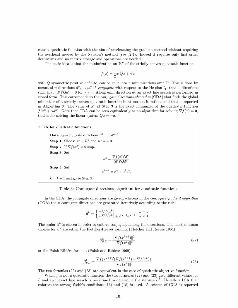
with Q symmetric positive definite, can be split into n minimizations over IR. This is done bymeans of n directions d0, . . . , dn−1 conjugate with respect to the Hessian Q, that is directionssuch that (dj) Qdi = 0 for j = i. Along each direction dj an exact line search is performed inclosed form. This corresponds to the conjugate directions algorithm (CDA) that finds the globalminimizer of a strictly convex quadratic function in at most n iterations and that is reportedin Algorithm 3. The value of αk at Step 3 is the exact minimizer of the quadratic functionf(xk + αdk). Note that CDA can be seen equivalently as an algorithm for solving ∇f(x) = 0,that is for solving the linear system Qx = −a.

CDA for quadratic functions

Data. Q−conjugate directions d0, . . . , dn−1.Step 1. Choose x0 ∈ Rn and set k = 0.Step 2. If ∇f(xk) = 0 stop.Step 3. Set

αk =∇f(xk) dk(dk) Qdk

.

Step 4. Setxk+1 = xk + αkdk,

k = k + 1 and go to Step 2.

Table 3: Conjugate directions algorithm for quadratic functions

In the CDA, the conjugate directions are given, whereas in the conjugate gradient algorithm(CGA) the n conjugate directions are generated iteratively according to the rule

dk =−∇f(xk) k = 0−∇f(xk) + βk−1dk−1 k ≥ 1.

The scalar βk is chosen in order to enforce conjugacy among the directions. The most commonchoices for βk are either the Fletcher-Reeves formula (Fletcher and Reeves 1964)

βkFR =∇f(xk+1) 2

∇f(xk) 2, (22)

or the Polak-Ribiere formula (Polak and Ribiere 1969)

βkPR =∇f(xk+1) (∇f(xk+1)−∇f(xk))

∇f(xk) 2. (23)

The two formulas (22) and (23) are equivalent in the case of quadratic objective function.When f is not a quadratic function the two formulas (22) and (23) give different values for

β and an inexact line search is performed to determine the stepsize αk. Usually a LSA thatenforces the strong Wolfe’s conditions (16) and (18) is used. A scheme of CGA is reported

10

CGA for nonlinear functions

Step 1. Choose x0 ∈ Rn and set k = 0.Step 2. If ∇f(xk) = 0 stop.Step 3. Compute βk−1 by either (22) or (23) and set the direction

dk =−∇f(xk) k = 0−∇f(xk) + βk−1dk−1 k ≥ 1;

Step 4. Find αk by means of a LSA that satisfies the strong Wolfe’s conditions (16)and (18).

Step 5. Setxk+1 = xk + αkdk,

k = k + 1 and go to Step 2.

Table 4: Conjugate gradient algorithm for nonlinear functions

in Algorithm 4. The simplest device used to guarantee global convergence properties of CGmethods is a periodic restart along the steepest descent direction. Restarting can also be usedto deal with the loss of conjugacy due to the presence of nonquadratic terms in the objectivefunction that may cause the method to generate inefficient or even meaningless directions.Usually the restart procedure occurs every n steps or if a test on the loss of conjugacy such as

|∇f(xk) ∇f(xk−1)| > δ ∇f(xk−1) 2,

with 0 < δ < 1, is satisfied.However, in practice, the use of a regular restart may not be the most convenient technique

for enforcing global convergence. Indeed CGA are used for large scale problems when n is verylarge and the expectation is to solve the problem in less than n iterations, that is before restartoccurs. Without restart, the CGA with βk = βkFR and a LSA that guarantees the satisfactionof the strong Wolfe’s conditions, is globally convergent in the sense that (13) holds (Al-Baali1985). Actually in Gilbert and Nocedal (1992) the same type of convergence has been provedfor any value of βk such that 0 < |βk| ≤ βkFR. Analogous convergence results do not hold forthe Polak-Ribiere formula even if the numerical performance of this formula is usually superiorto Fletcher-Reeves one. This motivated a big effort to find a globally convergent version ofthe Polak-Ribiere method. Indeed condition (13) can be established for a modification of thePolak-Ribiere CG method that uses only positive values of βk = maxβkPR, 0 and a LSA thatensures satisfaction of the strong Wolfe’s conditions and of the additional condition

∇f(xk) dk ≤ −c ∇f(xk) 2

for some constant c > 0 (Powell 1986).Recently it has been proved that the Polak-Ribiere CG method satisfies the stronger convergencecondition (12) if a a more sophisticated line search technique is used (Grippo and Lucidi 1997).Indeed a LSA that enforces condition (19) coupled with a sufficient descent condition of thetype

−δ2 ∇f(xk+1) 2 ≤ ∇f(xk+1) dk+1 ≤ −δ1 ∇f(xk+1) 2

with 0 < δ1 < 1 < δ2 must be used.With respect to the numerical performance, the CGA is also affected by the condition

number of the Hessian ∇2f . This leads to the use of preconditioned conjugate gradient methodsand many papers have been devoted to the study of efficient preconditioners.

11

2.4 Newton’s Methods

The Newton’s method is considered one of the most powerful algorithms for solving uncon-strained optimization problems (see (More and Sorensen 1984) for a review). It relies on thequadratic approximation

qk(s) =1

2s ∇2f(xk)s+∇f(xk) s+ f(xk)

of the objective function f in the neighborhood of the current iterate xk and requires thecomputation of ∇f and ∇2f at each iteration k. Newton’s direction dkN is obtained as astationary point of the quadratic approximation qk, that is as a solution of the system:

∇2f(xk)dN = −∇f(xk). (24)

Provided that ∇2f(xk) is non-singular, Newton’s direction is given by dkN =−[∇2f(xk)]−1∇f(xk) and the basic algorithmic scheme is defined by the iteration

xk+1 = xk − [∇2f(xk)]−1∇f(xk); (25)

we refer to (25) as the pure Newton’s method. The reputation of Newton’s method is due to thefact that, if the starting point x0 is close enough to a solution x∗, then the sequence generatedby iteration (25) converges to x∗ superlinearly (quadratically if the Hessian ∇2f is Lipschitzcontinuous in a neighborhood of the solution).

However, the pure Newton’s method presents some drawbacks. Indeed ∇2f(xk) may besingular, and hence Newton’s direction cannot be defined; the starting point x0 can be suchthat the sequence xk generated by iteration (25) does not converge and even convergence toa maximum point may occur. Therefore, the pure Newton’s method requires some modificationthat enforces the global convergence to a solution, preserving the rate of convergence. A globallyconvergent Newton’s method must produce a sequence xk such that: (i) it admits a limit point;(ii) any limit point belongs to the level set L0 and is a stationary point of f ; (iii) no limit pointis a maximum point of f ; (iv) if x∗ is a limit point of xk and ∇2f(x∗) is positive definite,then the convergence rate is at least superlinear.

There are two main approaches for designing globally convergent Newton’s method, namelythe line search approach and the trust region approach. We briefly describe them in the nexttwo sections.

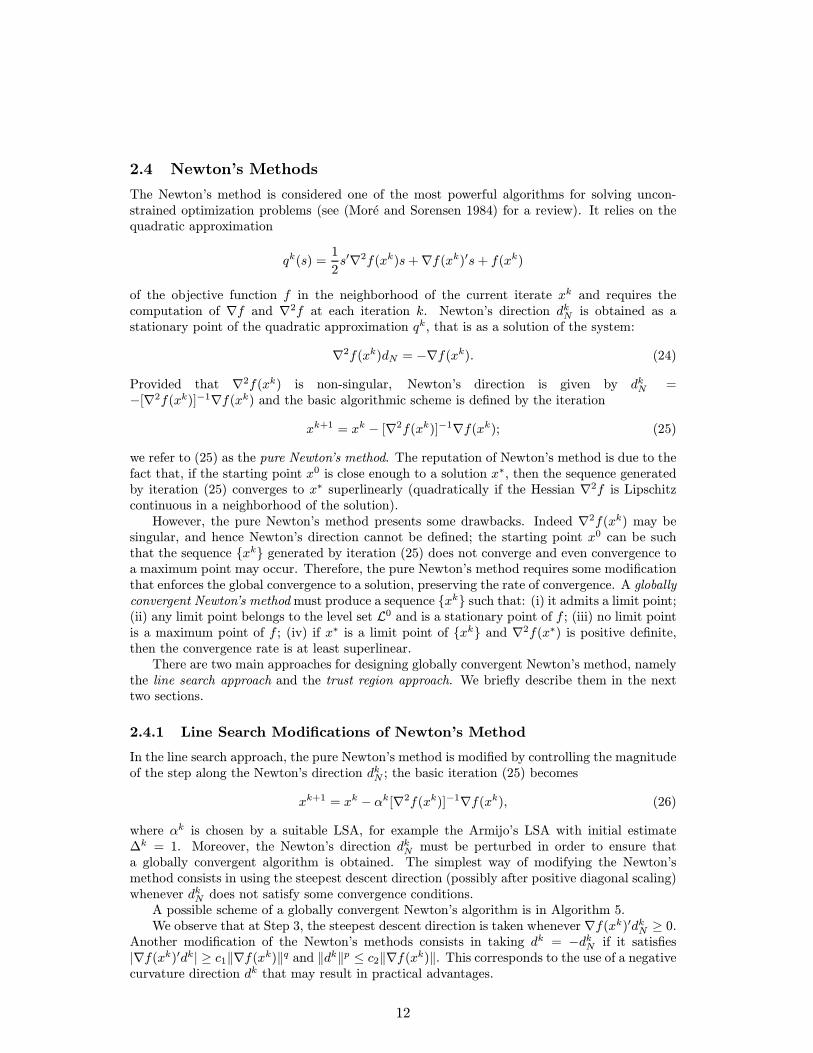
2.4.1 Line Search Modifications of Newton’s Method

In the line search approach, the pure Newton’s method is modified by controlling the magnitudeof the step along the Newton’s direction dkN ; the basic iteration (25) becomes

xk+1 = xk − αk[∇2f(xk)]−1∇f(xk), (26)

where αk is chosen by a suitable LSA, for example the Armijo’s LSA with initial estimate∆k = 1. Moreover, the Newton’s direction dkN must be perturbed in order to ensure thata globally convergent algorithm is obtained. The simplest way of modifying the Newton’smethod consists in using the steepest descent direction (possibly after positive diagonal scaling)whenever dkN does not satisfy some convergence conditions.

A possible scheme of a globally convergent Newton’s algorithm is in Algorithm 5.We observe that at Step 3, the steepest descent direction is taken whenever ∇f(xk) dkN ≥ 0.

Another modification of the Newton’s methods consists in taking dk = −dkN if it satisfies|∇f(xk) dk| ≥ c1 ∇f(xk) q and dk p ≤ c2 ∇f(xk) . This corresponds to the use of a negativecurvature direction dk that may result in practical advantages.

12

Line search based Newton’s method

Data. c1 > 0, c2 > 0, p ≥ 2, q ≥ 3.Step 1. Choose x0 ∈ IRn and set k = 0.Step 2. If ∇f(xk) = 0 stop.Step 3. If a solution dkN of the system

∇2f(xk)dN = −∇f(xk)exists and satisfies the conditions

∇f(xk) dkN ≤ −c1 ∇f(xk) q, dkNp ≤ c2 ∇f(xk)

then set the direction dk = dkN ; otherwise set dk = −∇f(xk).

Step 4. Find αk by using the Armjio’s LSA of Algorithm 1.

Step 5. Setxk+1 = xk + αkdk,

k = k + 1 and go to Step 2.

Table 5: Line search based Newton’s method

The use of the steepest descent direction is not the only possibility to construct globallyconvergent modifications of Newton’s method. Another way is that of perturbing the Hessianmatrix ∇2f(xk) by a diagonal matrix Y k so that the matrix ∇2f(xk) + Y k is positive definiteand a solution d of the system

(∇2f(xk) + Y k)d = −∇f(xk) (27)

exists and provides a descent direction. A way to construct such perturbation is to use amodified Cholesky factorization (see e.g. Gill et al. (1981), Lin and More (1999)).

The most common versions of globally convergent Newton’s methods are based on the en-forcement of a monotonic decrease of the objective function values, although neither strongtheoretical reasons nor computational evidence support this requirement. Indeed, the conver-gence region of Newton’s method is often much larger than one would expect, but a convergentsequence in this region does not necessarily correspond to a monotonically decreasing sequenceof function values. It is possible to relax the standard line search conditions in a way that pre-serves a global convergence property. More specifically in Grippo et al. (1986) a modificationof the Newton’s method that uses the Armijo-type nonmonotone rule (20) has been proposed.The algorithmic scheme remains essentially the same of Algorithm 5 except for Step 4. It isreported in Algorithm 6.

Actually, much more sophisticated nonmonotone stabilization schemes have been proposed(Grippo et al. 1991). We do not go into detail about these schemes. However, it is worthwhileto remark that, at each iteration of these schemes only the magnitude of dk is checked andif the test is satisfied, the stepsize one is accepted without evaluating the objective function.Nevertheless, a test on the decrease of the values of f is performed at least every M steps.

The line search based Newton’s methods described so far converge in general to pointssatisfying only the first order NOC for Problem (2). This is essentially due to the fact thatNewton’s method does not exploit all the information contained in the second derivatives.Indeed stronger convergence results can be obtained by using the pair of directions (dk, sk) andusing a curvilinear line search, that is a line search along the curvilinear path

xk+1 = xk + αkdk + (αk)1/2sk, (28)

13

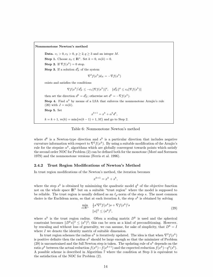
Nonmonotone Newton’s method

Data. c1 > 0, c2 > 0, p ≥ 2, q ≥ 3 and an integer M .Step 1. Choose x0 ∈ IRn. Set k = 0, m(k) = 0.Step 2. If ∇f(xk) = 0 stop.Step 3. If a solution dkN of the system

∇2f(xk)dN = −∇f(xk)exists and satisfies the conditions

∇f(xk) dkN ≤ −c1 ∇f(xk) q, dkNp ≤ c2 ∇f(xk)

then set the direction dk = dkN ; otherwise set dk = −∇f(xk).

Step 4. Find αk by means of a LSA that enforces the nonmonotone Armjio’s rule(20) with J = m(k).

Step 5. Setxk+1 = xk + αkdk,

k = k + 1, m(k) = minm(k − 1) + 1,M and go to Step 2.

Table 6: Nonmonotone Newton’s method

where dk is a Newton-type direction and sk is a particular direction that includes negativecurvature information with respect to∇2f(xk). By using a suitable modification of the Armjio’srule for the stepsize αk, algorithms which are globally convergent towards points which satisfythe second order NOC for Problem (2) can be defined both for the monotone (More and Sorensen1979) and the nonmonotone versions (Ferris et al. 1996).

2.4.2 Trust Region Modifications of Newton’s Method

In trust region modifications of the Newton’s method, the iteration becomes

xk+1 = xk + sk,

where the step sk is obtained by minimizing the quadratic model qk of the objective functionnot on the whole space IRn but on a suitable “trust region” where the model is supposed tobe reliable. The trust region is usually defined as an p-norm of the step s. The most commonchoice is the Euclidean norm, so that at each iteration k, the step sk is obtained by solving

mins∈IRn

12s ∇2f(xk)s+∇f(xk) ss 2 ≤ (ak)2, (29)

where ak is the trust region radius. Often a scaling matrix Dk is used and the sphericalconstraint becomes Dks 2 ≤ (ak)2; this can be seen as a kind of preconditioning. However,by rescaling and without loss of generality, we can assume, for sake of simplicity, that Dk = Iwhere I we denote the identity matrix of suitable dimension.

In trust region schemes the radius ak is iteratively updated. The idea is that when ∇2f(xk)is positive definite then the radius ak should be large enough so that the minimizer of Problem(29) is unconstrained and the full Newton step is taken. The updating rule of ak depends on theratio ρk between the actual reduction f(xk)−f(xk+1) and the expected reduction f(xk)−qk(sk).A possible scheme is described in Algorithm 7 where the condition at Step 3 is equivalent tothe satisfaction of the NOC for Problem (2).

14

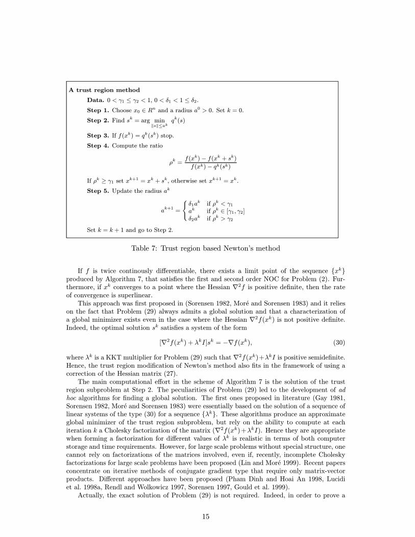
A trust region method

Data. 0 < γ1 ≤ γ2 < 1, 0 < δ1 < 1 ≤ δ2.

Step 1. Choose x0 ∈ Rn and a radius a0 > 0. Set k = 0.Step 2. Find sk = arg min

s ≤akqk(s)

Step 3. If f(xk) = qk(sk) stop.

Step 4. Compute the ratio

ρk =f(xk)− f(xk + sk)f(xk)− qk(sk)

If ρk ≥ γ1 set xk+1 = xk + sk, otherwise set xk+1 = xk.

Step 5. Update the radius ak

ak+1 =δ1a

k if ρk < γ1ak if ρk ∈ [γ1, γ2]δ2a

k if ρk > γ2

Set k = k + 1 and go to Step 2.

Table 7: Trust region based Newton’s method

If f is twice continously differentiable, there exists a limit point of the sequence xkproduced by Algorithm 7, that satisfies the first and second order NOC for Problem (2). Fur-thermore, if xk converges to a point where the Hessian ∇2f is positive definite, then the rateof convergence is superlinear.

This approach was first proposed in (Sorensen 1982, More and Sorensen 1983) and it relieson the fact that Problem (29) always admits a global solution and that a characterization ofa global minimizer exists even in the case where the Hessian ∇2f(xk) is not positive definite.Indeed, the optimal solution sk satisfies a system of the form

[∇2f(xk) + λkI]sk = −∇f(xk), (30)

where λk is a KKT multiplier for Problem (29) such that ∇2f(xk)+λkI is positive semidefinite.Hence, the trust region modification of Newton’s method also fits in the framework of using acorrection of the Hessian matrix (27).

The main computational effort in the scheme of Algorithm 7 is the solution of the trustregion subproblem at Step 2. The peculiarities of Problem (29) led to the development of adhoc algorithms for finding a global solution. The first ones proposed in literature (Gay 1981,Sorensen 1982, More and Sorensen 1983) were essentially based on the solution of a sequence oflinear systems of the type (30) for a sequence λk. These algorithms produce an approximateglobal minimizer of the trust region subproblem, but rely on the ability to compute at eachiteration k a Cholesky factorization of the matrix (∇2f(xk)+λkI). Hence they are appropriatewhen forming a factorization for different values of λk is realistic in terms of both computerstorage and time requirements. However, for large scale problems without special structure, onecannot rely on factorizations of the matrices involved, even if, recently, incomplete Choleskyfactorizations for large scale problems have been proposed (Lin and More 1999). Recent papersconcentrate on iterative methods of conjugate gradient type that require only matrix-vectorproducts. Different approaches have been proposed (Pham Dinh and Hoai An 1998, Lucidiet al. 1998a, Rendl and Wolkowicz 1997, Sorensen 1997, Gould et al. 1999).

Actually, the exact solution of Problem (29) is not required. Indeed, in order to prove a

15

global convergence result of a trust region scheme, it suffices that the model value qk(sk) is notlarger than the model value at the Cauchy point, which is the minimizer of the quadratic modelwithin the trust region along the (preconditioned) steepest-descent direction (Powell 1975).Hence any descent method that moves from the Cauchy point ensures convergence (Toint 1981,Steihaug 1983).

2.4.3 Truncated Newton’s Methods

Newton’s method requires at each iteration k the solution of a system of linear equations. Inthe large scale setting, solving exactly the Newton’s system can be too burdensome and storingor factoring the full Hessian matrix can be difficult when not impossible. Moreover the exactsolution when xk is far from a solution and ∇f(xk) is large may be unnecessary. On thebasis of these remarks, inexact Newton’s methods have been proposed (Dembo et al. 1982) thatapproximately solve the Newton system (24) and still retain a good convergence rate. If dkN isany approximate solution of the Newton system (24), the measure of accuracy is given by theresidual rk of the Newton equation, that is

rk = ∇2f(xk)dkN +∇f(xk).By controlling the magnitude of rk, superlinear convergence can be proved: if xk convergesto a solution and if

limk→∞

rk

∇f(xk) = 0, (31)

then xk converges superlinearly. This result is at the basis of Truncated Newton’s methods(see Nash (1999) for a recent survey).

Truncated Newton’s Algorithm (TNA)

Data. k, H, g and a scalar η > 0.

Step 1. Set ε = η g min1

k + 1, g , i = 0.

p0 = 0, r0 = −g, s0 = r0 ,Step 2. If (si) Hsi ≤ 0, set dN = −g if i = 0

pi if i > 0and stop.

Step 3. Compute αi =(si) ri

(si) Hsiand set

pi+1 = pi + αisi,ri+1 = ri − αiHsi,

Step 4. If ri+1 > ε , compute βi =ri+1 2

ri 2, set

si+1 = ri+1 + βisi,

i = i+ 1 and go to Step 2;

Step 5. Set dN = pi+1 and stop.

Table 8: Truncated Newton’s Algorithm

These methods require only matrix-vector products and hence they are suitable for largescale problems. The classical truncated Newton’s method (TNA) (Dembo and Steihaug 1983)

16

was thought for the case of positive definite Hessian ∇2f(xk). It is obtained by applying aCG scheme to find an approximate solution dkN to the linear system (24). We refer to outeriterations k for the sequence of points xk and to inner iterations i for the iterations of theCG scheme applied to the solution of system (24).The inner CG scheme generates vectors diN that iteratively approximate the Newton directiondkN . It stops either if the corresponding residual r

i = ∇2f(xk)diN +∇f(xk) satisfies ri ≤ εk,where εk > 0 is such to enforce (31), or if a non positive curvature direction is found, that is ifa conjugate direction si is generated such that

(si) ∇2f(xk)si ≤ 0. (32)

The same convergence results of Newton’s method hold, and if the smallest eigenvalue of∇2f(xk) is sufficiently bounded away from zero, the rate of convergence is still superlinear.We report in Algorithm 8 the inner CG method for finding an approximate solution of sys-tem (24). For sake of simplicity, we eliminate the dependencies on iteration k and we setH = ∇2f(xk), g = ∇f(xk). The method generates conjugate directions si and vectors pi thatapproximate the solution dkN of the Newton’s system.

By applying TNA to find an approximate solution of the linear system at Step 3 of Al-gorithm 5 (Algorithm 6) we obtain the monotone (nonmonotone) truncated version of theNewton’s method.

In Grippo et al. (1989) a more general Truncated Newton’s algorithm based on a CGmethod has been proposed. The algorithm attempts to find a good approximation of theNewton direction even if ∇2f(xk) is not positive definite. Indeed it does not stop when anegative curvature direction is encountered and this direction is used to construct additionalvectors that allow us to proceed in the CG scheme. Of course this Negative Curvature TruncatedNewton’s Algorithm (NCTNA) encompasses the standard TNA.

For sake of completeness, we remark that, also in the truncated setting, it is possible todefine a class of line search based algorithms which are globally convergent towards points whichsatisfy second order NOC for Problem (2). This is done by using a curvilinear line search (28)with dk and sk obtained by a Lanczos based iterative scheme. These algorithms were shown tobe very efficient in solving large scale unconstrained problems (Lucidi and Roma 1997, Lucidiet al. 1998b).

2.5 Quasi-Newton Methods

Quasi-Newton methods were introduced with the aim of defining efficient methods that do notrequire the evaluation of second order derivatives. They are obtained by setting dk as thesolution of

Bkd = −∇f(xk), (33)

where Bk is a n × n symmetric and positive definite matrix which is adjusted iteratively insuch a way that the direction dk tends to approximate the Newton direction. Formula (33) isreferred to as the direct quasi-Newton formula; in turn the inverse quasi-Newton formula is

dk = −Hk∇f(xk).

The idea at the basis of quasi-Newton methods is that of obtaining the curvature informationnot from the Hessian but only from the values of the function and its gradient. The matrixBk+1 (Hk+1) is obtained as a correction of Bk (Hk), namely as Bk+1 = Bk +∆Bk (Hk+1 =Hk +∆Hk). Let us denote by

δk = xk+1 − xk, γk = ∇f(xk+1)−∇f(xk).

17

Taking into account that, in the case of quadratic function, the so called quasi-Newton equation

∇2f(xk)δk = γk (34)

holds, the correction ∆Bk (∆Hk ) is chosen such that

(Bk +∆Bk)δk = γk, (δk = (Hk +∆Hk)γk).

Methods differ in the way they update the matrix Bk (Hk). Essentially they are classifiedaccording to a rank one or a rank two updating formula.

BFGS inverse quasi-Newton method

Step 1. Choose x0 ∈ IRn. Set H0 = I and k = 0.

Step 2. If ∇f(xk) = 0 stop.Step 3. Set the direction

dk = −Hk∇f(xk);Step 4. Find αk by means of a LSA that satisfies the strong Wolfe’s conditions (16)and (18).

Step 5. Setxk+1 = xk + αkdk,Hk+1 = Hk +∆Hk

with ∆Hk given by (35) with ϕ = 1.

Set k = k + 1 and go to Step 2.

Table 9: Quasi-Newton BFGS algorithm

The most used class of quasi-Newton methods is the rank two Broyden class. The updatingrule of the matrix Hk is given by the following correction term

∆Hk =δk(δk)

(δk) γk− H

kγk(Hkγk)

(γk) Hkγk+ c (γk) Hkγk vk(vk) , (35)

where

vk =δk

(δk) γk− Hkγk

(γk) Hkγk,

and c is a nonnegative scalar. For c = 0 we have the Davidon-Fletcher-Powell (DFP) formula(Davidon 1959, Fletcher and Powell 1963) whereas for c = 1 we have the Broyden-Fletcher-Goldfarb-Shanno (BFGS) formula (Broyden 1970, Fletcher 1970b, Goldfarb 1970, Shanno 1970).An important property of methods in the Broyden class is that if H0 is positive definite and foreach k it results (δk) γk > 0, then positive definiteness is maintained for all the matrices Hk.

The BFGS method has been generally considered most effective. The BFGS method is aline search method, where the stepsize αk is obtained by a LSA that enforces the strong Wolfeconditions (16) and (18). We describe a possible scheme of the inverse BFGS algorithm inAlgorithm 9.

As regards convergence properties of quasi-Newton methods, satisfactory results exist forthe convex case (Powell 1971, 1976, Byrd et al. 1987). In the non-convex case, only partialresults exist. In particular, if there exists a constant ρ such that for every k

γk 2

(γk) δk≤ ρ, (36)

18

then the sequence xk generated by the BFGS algorithm satisfies condition (13) (Powell 1976).Condition (36) holds in the convex case.

A main result on the rate of convergence of quasi-Newton methods is given in the followingproposition (Dennis and More 1974).

Proposition 2.4 Let Bk be a sequence of non singular matrices and let xk be given by

xk+1 = xk − (Bk)−1∇f(xk).

Assume that xk converges to a point x∗ where ∇2f(x∗) is non singular. Then, the sequencexk converges superlinearly to x∗ if and only if

limk→∞

(Bk −∇2f(x∗))(xk+1 − xk)xk+1 − xk = 0.

For large scale problems forming and storing the matrix Bk (Hk) may be impracticableand limited memory quasi-Newton methods have been proposed. These methods use the in-formation of the last few iterations for defining an approximation of the Hessian avoiding thestorage of matrices. Among limited memory quasi-Newton methods, by far the most used isthe Limited memory BFGS method (L-BFGS). In the L-BFGS method the matrix Hk is notformed explicitely and only pairs of vectors (δk, γk) are stored that define Hk implicitly. Theproduct Hk∇f(xk) is obtained by performing a sequence of inner products involving ∇f(xk)and the M most recent pairs (δk, γk). Usually small values of M (3 ≤M ≤ 7) give satisfactoryresults, hence the method results to be very efficient for large scale problems (Liu and Nocedal1989, Nash and Nocedal 1991).

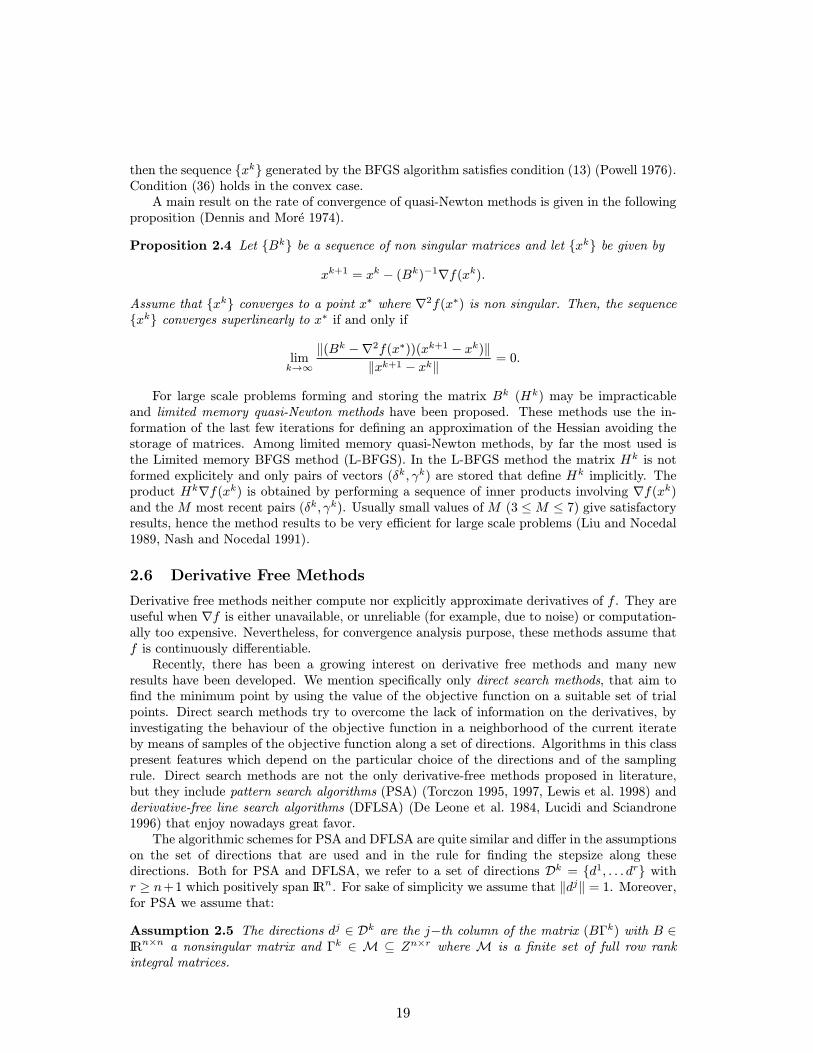
2.6 Derivative Free Methods

Derivative free methods neither compute nor explicitly approximate derivatives of f . They areuseful when ∇f is either unavailable, or unreliable (for example, due to noise) or computation-ally too expensive. Nevertheless, for convergence analysis purpose, these methods assume thatf is continuously differentiable.

Recently, there has been a growing interest on derivative free methods and many newresults have been developed. We mention specifically only direct search methods, that aim tofind the minimum point by using the value of the objective function on a suitable set of trialpoints. Direct search methods try to overcome the lack of information on the derivatives, byinvestigating the behaviour of the objective function in a neighborhood of the current iterateby means of samples of the objective function along a set of directions. Algorithms in this classpresent features which depend on the particular choice of the directions and of the samplingrule. Direct search methods are not the only derivative-free methods proposed in literature,but they include pattern search algorithms (PSA) (Torczon 1995, 1997, Lewis et al. 1998) andderivative-free line search algorithms (DFLSA) (De Leone et al. 1984, Lucidi and Sciandrone1996) that enjoy nowadays great favor.

The algorithmic schemes for PSA and DFLSA are quite similar and differ in the assumptionson the set of directions that are used and in the rule for finding the stepsize along thesedirections. Both for PSA and DFLSA, we refer to a set of directions Dk = d1, . . . dr withr ≥ n+1 which positively span IRn. For sake of simplicity we assume that dj = 1. Moreover,for PSA we assume that:

Assumption 2.5 The directions dj ∈ Dk are the j−th column of the matrix (BΓk) with B ∈IRn×n a nonsingular matrix and Γk ∈ M ⊆ Zn×r where M is a finite set of full row rankintegral matrices.

19

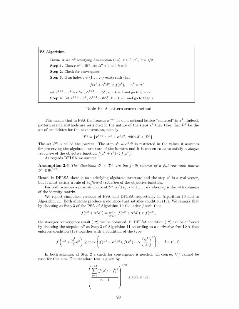
PS Algorithm

Data. A set Dk satisfying Assumption (2.5), τ ∈ 1, 2, θ = 1/2.Step 1. Choose x0 ∈ IRn, set ∆0 > 0 and k = 0;

Step 2. Check for convergence.

Step 3. If an index j ∈ 1, . . . , r exists such thatf(xk + αkdj) < f(xk), αk = ∆k

set xk+1 = xk + αkdj , ∆k+1 = τ∆k, k = k + 1 and go to Step 2.

Step 4. Set xk+1 = xk, ∆k+1 = θ∆k, k = k + 1 and go to Step 2.

Table 10: A pattern search method

This means that in PSA the iterates xk+1 lie on a rational lattice “centered” in xk. Indeed,pattern search methods are restricted in the nature of the steps sk they take. Let Pk be theset of candidates for the next iteration, namely

Pk = xk+1 : xk + αkdj , with dj ∈ Dk.The set Pk is called the pattern. The step sk = αkdj is restricted in the values it assumesfor preserving the algebraic structure of the iterates and it is chosen so as to satisfy a simplereduction of the objective function f(xk + sk) < f(xk).

As regards DFLSA we assume

Assumption 2.6 The directions dj ∈ Dk are the j−th column of a full row rank matrixBk ∈ IRn×r.Hence, in DFLSA there is no underlying algebraic structure and the step sk is a real vector,but it must satisfy a rule of sufficient reduction of the objective function.

For both schemes a possible choice of Dk is ±ej , j = 1, . . . , n where ej is the j-th columnsof the identity matrix.

We report simplified versions of PSA and DFLSA respectively in Algorithm 10 and inAlgorithm 11. Both schemes produce a sequence that satisfies condition (13). We remark thatby choosing at Step 3 of the PSA of Algorithm 10 the index j such that

f(xk + αkdj) = mini∈Dk

f(xk + αkdi) < f(xk),

the stronger convergence result (12) can be obtained. In DFLSA condition (12) can be enforcedby choosing the stepsize αk at Step 3 of Algorithm 11 according to a derivative free LSA thatenforces condition (19) together with a condition of the type

f xk +αk

δdk ≥ max f(xk + αkdk), f(xk)− γ αk

δ

2

, δ ∈ (0, 1).

In both schemes, at Step 2 a check for convergence is needed. Of course, ∇f cannot beused for this aim. The standard test is given by

n+1

i=1

(f(xi)− f)2

n+ 1

1/2

≤ tolerance,

20

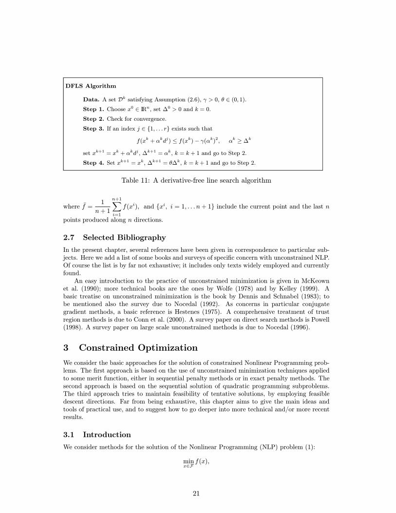
DFLS Algorithm

Data. A set Dk satisfying Assumption (2.6), γ > 0, θ ∈ (0, 1).Step 1. Choose x0 ∈ IRn, set ∆0 > 0 and k = 0.

Step 2. Check for convergence.

Step 3. If an index j ∈ 1, . . . r exists such thatf(xk + αkdj) ≤ f(xk)− γ(αk)2, αk ≥ ∆k

set xk+1 = xk + αkdj , ∆k+1 = αk, k = k + 1 and go to Step 2.

Step 4. Set xk+1 = xk, ∆k+1 = θ∆k, k = k + 1 and go to Step 2.

Table 11: A derivative-free line search algorithm

where f =1

n+ 1

n+1

i=1

f(xi), and xi, i = 1, . . . n+ 1 include the current point and the last npoints produced along n directions.

2.7 Selected Bibliography

In the present chapter, several references have been given in correspondence to particular sub-jects. Here we add a list of some books and surveys of specific concern with unconstrained NLP.Of course the list is by far not exhaustive; it includes only texts widely employed and currentlyfound.

An easy introduction to the practice of unconstrained minimization is given in McKeownet al. (1990); more technical books are the ones by Wolfe (1978) and by Kelley (1999). Abasic treatise on unconstrained minimization is the book by Dennis and Schnabel (1983); tobe mentioned also the survey due to Nocedal (1992). As concerns in particular conjugategradient methods, a basic reference is Hestenes (1975). A comprehensive treatment of trustregion methods is due to Conn et al. (2000). A survey paper on direct search methods is Powell(1998). A survey paper on large scale unconstrained methods is due to Nocedal (1996).

3 Constrained Optimization

We consider the basic approaches for the solution of constrained Nonlinear Programming prob-lems. The first approach is based on the use of unconstrained minimization techniques appliedto some merit function, either in sequential penalty methods or in exact penalty methods. Thesecond approach is based on the sequential solution of quadratic programming subproblems.The third approach tries to maintain feasibility of tentative solutions, by employing feasibledescent directions. Far from being exhaustive, this chapter aims to give the main ideas andtools of practical use, and to suggest how to go deeper into more technical and/or more recentresults.

3.1 Introduction

We consider methods for the solution of the Nonlinear Programming (NLP) problem (1):

minx∈F

f(x),

21

where x ∈ IRn is a vector of decision variables, f : IRn → IR is an objective function, and thefeasible set F is described by inequality and/or equality constraints on the decision variables :

F = x ∈ IRn : gi(x) ≤ 0, i = 1, . . . , p; hj(x) = 0, j = 1, . . . ,m, m ≤ n;

that is, we consider methods for the solution of the constrained NLP problem (3):

minx∈IRn

f(x)

g(x) ≤ 0h(x) = 0,

where g : IRn → IRp, and h : IRn → IRm, with m ≤ n.Here, for simplicity, the problem functions f, g, h are twice continuously differentiable in

IRn, even if in many cases they need to be only once continuously differentiable.

For the solution of Problem (3) two main approaches have been developed. Since, inprinciple, an unconstrained minimization is simpler then a constrained minimization, the firstapproach is based on the transformation of the constrained problem into a sequence of uncon-strained problems, or even into a single unconstrained problem. Basic tools for this approachare the unconstrained minimization methods of Section 2. The second approach is based onthe transformation of the constrained problem into a sequence of simpler constrained problems,that is either linear or quadratic programming problems; thus the basic tools become the algo-rithms considered in this volume for linear or quadratic programming. Due to space limits, wewill confine ourselves to methods based on quadratic programming, that are by far most widelyemployed.

We do not treat problems with special structure, such as bound and/or linearly constrainedproblems, for which highly specialized algorithms exist.

We employ the additional notation maxy, z, where y, z ∈ IRp, denotes the vector withcomponents maxyi, zi for i = 1, . . . , p.

3.2 Unconstrained Sequential Methods

In this section we consider methods that are very basic in NLP. These are: the quadratic penaltymethod, which belongs to the class of exterior penalty functions methods, the logarithmic barriermethod, which belongs to the class of interior penalty functions or barrier functions methods,and the augmented Lagrangian method, which can be considered as an improved exterior penaltymethod.

3.2.1 The Quadratic Penalty Method

The quadratic penalty method dates back to an idea of Courant (1943), that has been fullydeveloped in the book by Fiacco and McCormick (1968). Let us consider Problem (3) and letp(x), p : IRn → IR be a continuous function such that p(x) = 0 for all x ∈ F , p(x) > 0 for allx /∈ F . Then, we can associate to Problem (3) the unconstrained problem:

minx∈IRn

[f(x) +1p(x)],

where > 0. The function

P (x; ) = f(x) +1p(x),

parameterized by the penalty parameter , is called a penalty function for Problem (3), since itis obtained by adding to the objective function of the original problem a term that penalizes the

22

constraint violations. It is called an exterior penalty function, because its minimizers are usuallyexterior to the feasible set F . The penalization of the constraint violations becomes more severeas the penalty parameter is smaller. Given a sequence of positive numbers k, k = 0, 1, . . .such that k+1 < k, limk→∞ k = 0, the exterior penalty method for solving Problem (3) isreported in Algorithm 12.

Exterior Penalty Function Algorithm

Data. k such that k+1 < k and limk→∞ k = 0.

Step 1. Choose xs ∈ IRn and set k = 0.Step 2. Starting from xs, find an unconstrained local minimizer

xk = arg minx∈IRn

P (x; k).

Step 3. If xk is a KKT point, then stop.

Step 4. Set xs = xk, k = k + 1 and go to Step 2.

Table 12: The exterior penalty function algorithm

Under weak assumptions, it can be proved that limit points of the sequence xk producedby the method of Algorithm 12 are local solutions of the constrained Problem (3).

The most widely used penalty function is the quadratic penalty function and the corre-sponding method is called the quadratic penalty method. The function P is obtained by usingpenalty terms that are the squares of the constraint violations and is given by:

P (x; ) = f(x) +1

maxg(x), 0 2 + h(x) 2 .

The quadratic penalty method is very simple; however it suffers from a main disadvantage:as becomes smaller, the Hessian matrix ∇2P (x; ) becomes more ill-conditioned, so that theunconstrained minimization of P (x; ) becomes more difficult and slow. To alleviate the effectsof ill-conditioning, the scheme of Algorithm 12 can be modified so that at Step 2 a startingpoint xs closer to xk than xk−1 can be given by extrapolating the trajectory of minimizersx0, x1, . . . xk−1. In any case, at present, the method has been overcome by methods based onthe augmented Lagrangian function.

As a final remark, the function P (x; ) is not twice continuously differentiable at pointswhere some constraint gi is active, due to the presence in P of the term maxgi, 0, and thismust be taken into account in the minimization of P .

3.2.2 The Logarithmic Barrier Method

The original idea of the logarithmic barrier method is due to Frisch (1955); again, in the bookby Fiacco and McCormick (1968) a comprehensive treatment was given.

This method can be employed for NLP problems with only inequality constraints, that is:

minx∈IRn

f(x)

g(x) ≤ 0. (37)

It is assumed, moreover, that the strictly feasible region

Fo = x ∈ IRn : gi(x) < 0, i = 1, . . . , p (38)

23

is nonempty.A barrier term for the feasible set F of Problem (37) is a continuous function v(x) defined

in Fo, and such that v(x)→∞ as x ∈ Fo approaches the boundary of F . Then, associated toProblem (37) we consider the unconstrained problem

minx∈Fo

[f(x) + v(x)],

where > 0. The functionV (x; ) = f(x) + v(x),

parameterized by , is called a barrier function for Problem (37), since it is obtained by addingto the objective function of the problem a term that establishes a barrier on the boundary ofthe feasible set, thus preventing that a descent path for V starting in the interior of F crossesthe boundary. The barrier is as sharper as the barrier parameter is larger. Algorithms basedon barrier functions are also called interior point algorithms because the sequences that areproduced are interior to the strictly feasible region.

Given a sequence of positive numbers k, k = 0, 1, . . . such that k+1 < k, andlimk→∞ k = 0, the barrier function method for solving Problem (37) is reported in Algo-rithm 13.

A Barrier Function Algorithm

Data. k such that k+1 < k and limk→∞ k = 0.

Step 1. Choose xs ∈ Fo and set k = 0.

Step 2. Starting from xs, find an unconstrained local minimizer

xk = arg minx∈Fo

V (x; k).

Step 3. If xk is a KKT point, then stop.

Step 4. Set xs = xk, k = k + 1 and go to Step 2.

Table 13: A barrier function algorithm

As for the quadratic penalty method, the convergence analysis of the method shows that,under weak assumptions, limit points of the sequence xk produced by the method in Algo-rithm 13 are local solutions of the constrained Problem (37).

The most important barrier function for Problem (37) is the logarithmic barrier function,and the corresponding method is called the logarithmic barrier method. The function V isobtained by using as barrier terms the natural logarithm of the constraints:

V (x; ) = f(x)−p

i=1

log(−gi(x)).

Also the logarithmic barrier method is very simple; however the same remarks made forthe quadratic penalty method hold. Namely, the method suffer of ill-conditioning as becomessmaller, and also in this case a better starting point xs can be found by extrapolating thetrajectory of minimizers x0, x1, . . .. An additional disadvantage is that xs must be strictlyfeasible, so that the feasibility subproblem must be considered solved at the beginning. Atpresent, the approach based on logarithmic barrier terms is not widely used for general NLPproblems. However in linearly constrained optimization it is of main importance to treat boundconstraints, and indeed it is at the basis of the interior points methods for linear and quadraticprogramming (see e.g. den Hertog (1994)).

24

Finally, we point out that the logarithmic barrier method can be combined with thequadratic penalty method to deal with problems with also equality constraints: in this case

a penalty term1h(x) 2 can be added to the function V , retaining the behaviour of both

approaches.

3.2.3 The Augmented Lagrangian Method

The augmented Lagrangian method has been proposed independently by Hestenes (1969) andPowell (1969) for the equality constrained problem; the extension to the inequality constrainedproblem is due to Rockafellar (1973). Miele et al. (1971, 1972) contributed to publicize themethod; in a series of papers that are at the core of his book, Bertsekas (1982) established thesuperiority of this method over the quadratic penalty method.

Let us consider first a NLP problem with only equality constraints:

minx∈IRn

f(x)

h(x) = 0.(39)

The Lagrangian function for Problem (39) is

L(x, µ) = f(x) + µ h(x). (40)

The augmented Lagrangian function for Problem (39) is the function

La(x, µ; ) = L(x, µ) +1h(x) 2, (41)

obtained by adding to L the quadratic penalty term for the constraint violations.The main property of function La is the following:

Proposition 3.1 Assume that x∗ is a local solution of Problem (39) that, together with themultiplier µ∗, satisfies the SOSC (restricted to equality constraints) given by Proposition 1.4of Section 1; then there exists a threshold value ∗ such that, for all ∈ (0, ∗], x∗ is a localsolution of the unconstrained problem

minx∈IRn

La(x, µ∗; ). (42)

Conversely, if for some µ∗ and , x∗ satisfies the SOSC to be a local solution of Problem (42)given by Proposition 1.4 of Section 1 , and h(x∗) = 0, then x∗ is a local solution of Problem(39), and µ∗ is the corresponding multiplier.

By Proposition 3.1 La(x, µ∗; k) can be employed in the quadratic penalty method of Al-

gorithm 12 in place of P (x; k), without requiring that k decreases to zero. It is required onlythat the condition k ≤ ∗ becomes fulfilled, thereby mitigating the ill-conditioning associatedwith the use of P . However, since µ∗ is not known in advance, a procedure that iterativelyupdates an estimate µk of µ∗ must be included in the method.

A generic algorithmic scheme of an augmented Lagrangian method for solving Problem (39)is in Algorithm 14.

The penalty parameter k+1 is usually set to ρ k, with ρ = 1 if h(xk) 2 is sufficientlysmaller than h(xk−1) 2, and ρ < 1 otherwise.

Updating formulas for the multiplier estimate are based on the fact that, under the assump-tions of Proposition 3.1, the pair (x∗, µ∗) is a saddle point of the function La, so that an ascentstrategy with respect to the dual function

Da(µ; ) = minx∈Bx∗

La(x, µ; ),

25

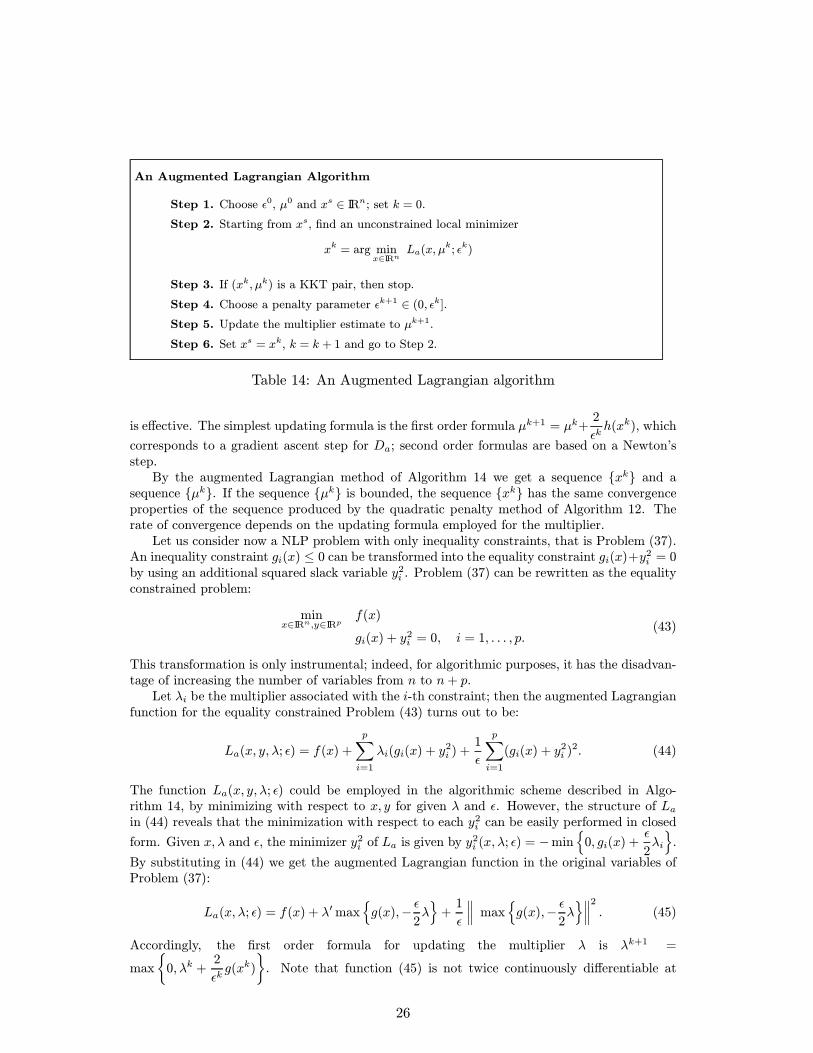
An Augmented Lagrangian Algorithm

Step 1. Choose 0, µ0 and xs ∈ IRn; set k = 0.Step 2. Starting from xs, find an unconstrained local minimizer

xk = arg minx∈IRn

La(x, µk; k)

Step 3. If (xk, µk) is a KKT pair, then stop.

Step 4. Choose a penalty parameter k+1 ∈ (0, k].

Step 5. Update the multiplier estimate to µk+1.

Step 6. Set xs = xk, k = k + 1 and go to Step 2.

Table 14: An Augmented Lagrangian algorithm

is effective. The simplest updating formula is the first order formula µk+1 = µk+2kh(xk), which

corresponds to a gradient ascent step for Da; second order formulas are based on a Newton’sstep.

By the augmented Lagrangian method of Algorithm 14 we get a sequence xk and asequence µk. If the sequence µk is bounded, the sequence xk has the same convergenceproperties of the sequence produced by the quadratic penalty method of Algorithm 12. Therate of convergence depends on the updating formula employed for the multiplier.

Let us consider now a NLP problem with only inequality constraints, that is Problem (37).An inequality constraint gi(x) ≤ 0 can be transformed into the equality constraint gi(x)+y2i = 0by using an additional squared slack variable y2i . Problem (37) can be rewritten as the equalityconstrained problem:

minx∈IRn,y∈IRp

f(x)

gi(x) + y2i = 0, i = 1, . . . , p.

(43)

This transformation is only instrumental; indeed, for algorithmic purposes, it has the disadvan-tage of increasing the number of variables from n to n+ p.

Let λi be the multiplier associated with the i-th constraint; then the augmented Lagrangianfunction for the equality constrained Problem (43) turns out to be:

La(x, y,λ; ) = f(x) +

p

i=1

λi(gi(x) + y2i ) +

1p

i=1

(gi(x) + y2i )2. (44)

The function La(x, y,λ; ) could be employed in the algorithmic scheme described in Algo-rithm 14, by minimizing with respect to x, y for given λ and . However, the structure of Lain (44) reveals that the minimization with respect to each y2i can be easily performed in closed

form. Given x,λ and , the minimizer y2i of La is given by y2i (x,λ; ) = −min 0, gi(x) +

2λi .

By substituting in (44) we get the augmented Lagrangian function in the original variables ofProblem (37):

La(x,λ; ) = f(x) + λ max g(x),−2λ +

1max g(x),−

2λ

2

. (45)

Accordingly, the first order formula for updating the multiplier λ is λk+1 =

max 0,λk +2kg(xk) . Note that function (45) is not twice continuously differentiable at

26

points where gi(x) = − 2λi for some i; however the lack of second order differentiability doesnot occur locally in a neighborhood of a KKT pair (x∗,λ∗) if g(x∗),λ∗ satisfy the strict com-plementarity condition.

Problems with both equality and inequality constraints can be handled by combining thetwo cases.

The augmented Lagrangian method with the first order multiplier updating is also referredto as the multiplier method. A less used term is the shifted barrier method.

Vast computational experience shows that the augmented Lagrangian function approachis reasonably effective, and many commercial softwares for the solution of NLP problems arebased on it.

3.3 Unconstrained Exact Penalty Methods

Exact penalty methods attempt to solve NLP problems by means of a single minimization of anunconstrained function, rather then by means of a sequence of unconstrained minimizations.Exact penalty methods are based on the construction of a function depending on a penaltyparameter > 0, such that the unconstrained minimum points of this function are also solutionsof the constrained problem for all values of in the interval (0, ∗], where ∗ is a threshold value.

We can subdivide exact penalty methods into two classes: methods based on exact penaltyfunctions and methods based on exact augmented Lagrangian functions. The term exact penaltyfunction is used when the variables of the unconstrained problem are the same of the originalconstrained problem, whereas the term exact augmented Lagrangian function is used whenthe unconstrained problem is defined in the product space of the problem variables and of themultipliers (primal and dual variables).

An exact penalty function, or an augmented Lagrangian function, possesses different exact-ness properties, depending on which kind of correspondence can be established, under suitableassumptions, between the set of the local (global) solutions of the constrained problem and theset of local (global) minimizers of the unconstrained function. Different definitions of exactnesscan be found in Di Pillo and Grippo (1989).

The simplest function that possesses exactness properties is obtained by adding to theobjective function the 1 norm of the constraint violations, weighted by a penalty parameter .The so-called 1 exact penalty function for Problem (3), introduced by Zangwill (1967), is givenby:

L1(x; ) = f(x) +1

p

i=0

maxgi(x), 0+m

j=1

|hj(x)| . (46)

In spite of its simplicity, function (46) is not continuously differentiable, so that its unconstrainedminimization cannot be performed using the techniques seen in Section 2 of this volume; oneshould resort to the less efficient nonsmooth optimization techniques.

Continuously differentiable exact penalty functions can be obtained from the augmentedLagrangian function of §3.2.3 by substituting the multiplier vectors λ, µ by continuously dif-ferentiable multiplier functions λ(x), µ(x), with the property that λ(x∗) = λ∗, µ(x∗) = µ∗

whenever the triplet (x∗,λ∗, µ∗) satisfies the KKT necessary conditions.For the equality constrained problem (39) a multiplier function is

µ(x) = −[∇h(x) ∇h(x)]−1∇h(x) ∇f(x);

then Fletcher’s exact penalty function, introduced in Fletcher (1970a), is:

UF (x; ) = f(x) + µ(x) h(x) +1h(x) 2. (47)

27

Similarly, for the inequality constrained problem (37) a multiplier function is:

λ(x) = −[∇g(x) ∇g(x) + θG2(x)]−1∇g(x) ∇f(x),

where θ > 0 and G(x) is the diagonal matrix with entries gi(x); an exact penalty function is(Glad and Polak 1979, Di Pillo and Grippo 1985):

U(x; ) = f(x) + λ (x)max g(x),−2λ(x) + max g(x),−

2λ(x)

2

. (48)

Exact augmented Lagrangian functions are obtained by incorporating in the augmentedLagrangian function La terms that penalize the violation of necessary optimality conditionsdifferent then feasibility. For instance, for the equality constrained problem (39) an exactaugmented Lagrangian function, studied by Di Pillo and Grippo (1979) is:

Sa(x, µ; ) = f(x) + µ h(x) +1h(x) 2 + θ ∇h(x) ∇xL(x, µ) 2, (49)

where θ > 0. It is evident that the last term in the r.h.s. of (49) penalizes in some way theviolation of the necessary optimality condition ∇xL(x, µ) = 0.

Exact penalty functions and exact augmented Lagrangian functions can also be endowedwith barrier terms that act on the boundary of a set that strictly contains the feasible set. Inthis way it is possible to build functions that not only have as unconstrained minimizers thesolution of the constrained problem, but have also compact level sets. Both these propertiesare quite important for the design of globally convergent algorithms. Indeed, making use ofthese functions it is possible to develop algorithms for constrained problems that behave likethe algorithms for unconstrained problems in terms of convergence and convergence rate, seefor instance Di Pillo et al. (1980, 1982, 1986).

Algorithms based on continuously differentiable exact penalty functions have not beenwidely implemented. This is mainly due to the fact that the evaluation of the multiplierfunction requires the inversion of a matrix of the dimension of the constraints vector. Morepromising is the use of exact augmented Lagrangian functions, even if their minimization mustbe performed on the enlarged space of the decision variables and of the multipliers.

Functions that possess exactness properties are also referred to as exact merit functionswhen they are used in sequential algorithms to measure the merit of subsequent iterates inmoving towards the solution of the constrained problem; in fact their minimization combinesthe often conflicting requirements of reducing both the objective function and the constraintviolations (and the violation of other NOC).

Exact penalty methods require in any case some strategy to select a penalty parametervalue in the interval (0, ∗] where exactness holds.

3.4 Sequential Quadratic Programming Methods

The sequential quadratic programming (SQP) approach can be viewed as a generalization toconstrained optimization of Newton’s method for unconstrained optimization: in fact it findsa step away from the current point by minimizing a quadratic model of the problem. TheSQP approach has been introduced by Wilson (1963); main developments are due to Garcia-Palomares and Mangasarian (1976), Han (1976, 1977), Powell (1978a,c,b).

For simplicity, let us consider the equality constrained Problem (39), with Lagrangianfunction (40). In principle, a solution of this problem could be found by solving w.r.t. (x, µ),the KKT first order NOC:

∇L(x, µ) = ∇f(x) +∇h(x)µh(x)

= 0. (50)

28

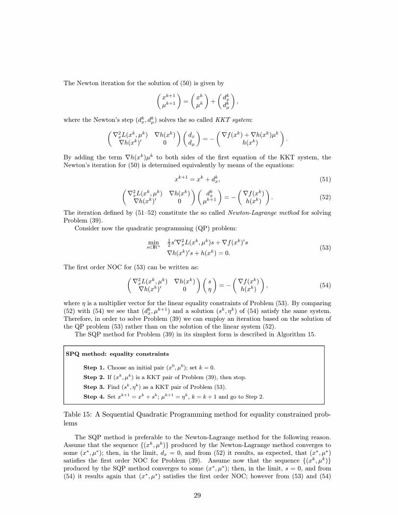
The Newton iteration for the solution of (50) is given by

xk+1

µk+1=

xk

µk+

dkxdkµ

,

where the Newton’s step (dkx, dkµ) solves the so called KKT system:

∇2xL(xk, µk) ∇h(xk)∇h(xk) 0

dxdµ

= − ∇f(xk) +∇h(xk)µkh(xk)

.

By adding the term ∇h(xk)µk to both sides of the first equation of the KKT system, theNewton’s iteration for (50) is determined equivalently by means of the equations:

xk+1 = xk + dkx, (51)

∇2xL(xk, µk) ∇h(xk)∇h(xk) 0

dkxµk+1

= − ∇f(xk)h(xk)

. (52)

The iteration defined by (51—52) constitute the so called Newton-Lagrange method for solvingProblem (39).

Consider now the quadratic programming (QP) problem:

mins∈IRn

12s ∇2xL(xk, µk)s+∇f(xk) s∇h(xk) s+ h(xk) = 0. (53)

The first order NOC for (53) can be written as:

∇2xL(xk, µk) ∇h(xk)∇h(xk) 0

sη

= − ∇f(xk)h(xk)

, (54)

where η is a multiplier vector for the linear equality constraints of Problem (53). By comparing(52) with (54) we see that (dkx, µ

k+1) and a solution (sk, ηk) of (54) satisfy the same system.Therefore, in order to solve Problem (39) we can employ an iteration based on the solution ofthe QP problem (53) rather than on the solution of the linear system (52).

The SQP method for Problem (39) in its simplest form is described in Algorithm 15.

SPQ method: equality constraints

Step 1. Choose an initial pair (x0, µ0); set k = 0.

Step 2. If (xk, µk) is a KKT pair of Problem (39), then stop.

Step 3. Find (sk, ηk) as a KKT pair of Problem (53).

Step 4. Set xk+1 = xk + sk; µk+1 = ηk, k = k + 1 and go to Step 2.

Table 15: A Sequential Quadratic Programming method for equality constrained prob-lems

The SQP method is preferable to the Newton-Lagrange method for the following reason.Assume that the sequence (xk, µk) produced by the Newton-Lagrange method converges tosome (x∗, µ∗); then, in the limit, dx = 0, and from (52) it results, as expected, that (x∗, µ∗)satisfies the first order NOC for Problem (39). Assume now that the sequence (xk, µk)produced by the SQP method converges to some (x∗, µ∗); then, in the limit, s = 0, and from(54) it results again that (x∗, µ∗) satisfies the first order NOC; however from (53) and (54)

29

we have also, in the limit, that s ∇2Lx(x∗, µ∗)s ≥ 0 for all s ∈ IRn such that ∇h(x∗) s = 0;therefore, in this case, (x∗, µ∗) satisfies also a second order NOC. In essence, the minimizationprocess of SQP drives the sequence toward beneficial KKT solutions.

Note that, thanks to the constraint, the objective function of the quadratic problem (53)could also be written as:

1

2s ∇2xL(xk, µk)s+∇xL(xk, µk) s+ L(xk, µk).

This leads to an alternative motivation of the SQP method. Indeed, Problem (39) can bewritten equivalently as

minx∈IRn

L(x, µ∗)

h(x) = 0,

where µ∗ is the KKT multiplier associated to the solution x∗ of (39). Then solving Problem(53) corresponds to finding (x∗, µ∗) by iteratively solving the problem of minimizing a quadraticapproximation of the Lagrangian L(x, µk) subject to a linear approximation of the constrainth(x) = 0.

The last observation suggests that the SQP framework can be extended easily to the generalNLP problem (3). Indeed, by linearizing also the inequality constraints we get the quadraticprogramming problem:

mins∈IRn

12s ∇2xL(xk,λk, µk)s+∇f(xk) s∇g(xk) s+ g(xk) ≤ 0∇h(xk) s+ h(xk) = 0.

(55)

The inequality constrained case puts in evidence an additional advantage of the SQP ap-proach over the Newton-Lagrange method: indeed it is much simpler to solve the QP subprob-lem (55) than to solve the set of equalities and inequalities obtained by linearizing the KKTconditions for Problem (3).

The SQP algorithm for Problem (3) is given in Algorithm 16.

SPQ method

Step 1. Choose an initial triplet (x0,λ0, µ0); set k = 0.

Step 2. If (xk,λk, µk) is a KKT triplet of Problem (3), then stop.

Step 3. Find (sk, ζk, ηk) as a KKT triplet of Problem (55).

Step 4. Set xk+1 = xk + sk; λk+1 = ζk; µk+1 = ηk, k = k + 1 and go to Step 2.

Table 16: A Sequential Quadratic Programming method for general constrained prob-lems

The equivalence between the SQP method and the Newton-Lagrange method provides thebasis for the main convergence and rate of converge results of the former.

Proposition 3.2 Assume that f , g, h are twice differentiable with Lipschitz continuous secondderivatives; assume that (x∗,λ∗, µ∗) satisfy the SOSC of Proposition 1.4 of Section 1 under strictcomplementarity between g(x∗) and λ∗. Then, there exists an open neighborhood B(x∗,λ∗,µ∗) suchthat, if (x0,λ0, µ0) ∈ B(x∗,λ∗,µ∗), the sequence (xk,λk, µk) produced by the SQP method is welldefined and converges to (x∗,λ∗, µ∗) with quadratic rate.

30

The SQP method outlined above requires the computation of the second order derivativesthat appear in ∇2xL(xk,λk, µk). As in the Newton’s method in unconstrained optimization,this can be avoided by substituting the Hessian matrix ∇2xL(xk,λk, µk) with a quasi-Newtonapproximation Bk, which is updated at each iteration. An obvious update strategy would beto define:

δk = xk+1 − xk, γk = ∇L(xk+1,λk, µk)−∇L(xk,λk, µk),and to update the matrix Bk by using the BFGS formula

Bk+1 = Bk +γk(γk)

(γk) δk− B

kδk(δk) Bk

(δk) Bkδk(56)

for unconstrained optimization. However, one of the properties that make the BFGS formulaappealing for unconstrained problems, that is maintenance of positive definiteness of Bk, is nolonger assured, since ∇2xL(x∗,λ∗, µ∗) is usually positive definite only on a subset of IRn. Thisdifficulty may be overcome by modifying γk as proposed by Powell (1978b). Let:

γk = τγk + (1− τ )Bkδk,where the scalar τ is defined as

τ =

1 if (δk) γk ≥ 0.2(δk) Bkδk

0.8(δk) Bkδk

(δk) Bkδk − (δk) γk if (δk) γk < 0.2(δk) Bkδk,

and update Bk by the damped BFGS formula, obtained by substituting γk for γk in (56); then,if Bk is positive definite the same holds for Bk+1. This ensures also that, if the quadraticprogramming problem is feasible, it admits a solution. Of course, by employing the quasi-Newton approximation, the rate of convergence becomes superlinear.

Proposition 3.2 states a local convergence result. If, as often happens, a point (x0,λ0, µ0) ∈B(x∗,λ∗,µ∗) is not known, the following difficulties have to be tackled:- at iteration k the QP subproblem may have no solution;

- the sequence (xk,λk, µk) may not be convergent.The first difficulty arises either because the quadratic objective function is unbounded from

below on the linearized feasible set, or because the linearized feasible set is empty. The first oc-currence can be avoided by substituting ∇2xL(xk,λk, µk) with a positive definite approximationBk, for instance as described before; or by employing the Hessian of the augmented Lagrangian∇2xLa(xk,λk, µk; ) in place of ∇2xL(xk,λk, µk). The second occurrence can be overcome bydefining a suitable relaxation of the QP subproblem so as to obtain a problem which is al-ways feasible, even if of larger dimension. As an example, the following subproblem has beenproposed (De O. Pantoja and Mayne 1991):

mins∈IRn,w∈IR

1

2s Bks+∇f(xk) s+ 1

εw

∇gi(xk) s+ gi(xk) ≤ w, i = 1, . . . , p

|∇hj(xk) s+ hj(xk)| ≤ w, j = 1, . . . ,mw ≥ 0,

(57)

where ε > 0 is a suitable penalty parameter. It is easy to verify that the feasible set of Problem(57) is not empty, so that, if Bk is positive definite, the problem admits a solution.

With respect to the convergence of the sequence (xk,λk, µk), we observe preliminarily thatif xk converges to some x∗ where the linear independence constraints qualification (LICQ)holds, then (λk, µk) also converges to some (λ∗, µ∗) such that (x∗,λ∗, µ∗) satisfies the KKT

31

NOC for Problem (3). In order to enforce the convergence of the sequence xk, in the sameline of the Newton’s method for unconstrained optimization, two strategies have been devisedwith reference to a suitable merit function associated with the NLP problem: the line searchapproach and the trust region approach. As said before, a merit function aims to reduce boththe objective function and the constraint violations (as well as the violation of other necessaryoptimality conditions); in this way it provides a measure of the progress toward a solution ofthe constrained problem.

3.4.1 The Line Search Approach

In the line search approach the sequence xk is given by the iteration:

xk+1 = xk + αksk,

where the direction sk is obtained by solving the k-th QP subproblem, and the stepsize αk

is evaluated so as to get a sufficient decrease of the merit function. A merit function widelyemployed in SQP methods is the 1 exact penalty function L1(x; ) given by (46). Although L1is not differentiable everywhere, it always has a directional derivative. It can be shown that,if the quadratic form in the QP subproblem is positive definite, and if the penalty parameterin L1 is sufficiently small, then s

k is a descent direction at xk for L1, so that an Armijo-likeline search along sk can be performed (Han 1977). However, due to its non differentiability,the merit function L1 suffers from a main drawback known as the Maratos effect (Maratos1978): even close to a solution, the stepsize αk = 1 may not be accepted, thus deteriorating theconvergence rate of the pure SQP method. To avoid the Maratos effect, different techniqueshave been proposed. Among them a curvilinear line search (Mayne and Polak 1982), basedon the formula xk+1 = xk + αksk + (αk)2sk, where the direction sk, that provides a secondorder correction, is evaluated so as to further reduce the constraint violations; and the watchdogtechnique (Chamberlain et al. 1982), based on nonmonotone strategies, by which we allow themerit function L1 to increase on certain iterations.

The Maratos effect can also be overcome by employing merit functions that are continuouslydifferentiable. For equality constraints, the use of Fletcher’s exact penalty function UF givenby (47) is usually referred (Powell and Yuan 1986); the extention to inequality constraints isbased on the exact penalty function U given in (48) (Di Pillo et al. 1992, Facchinei 1997). Itcan be shown that for a sufficiently small value of the penalty parameter , sk gives a descentdirection for the continuously differentiable exact penalty functions at xk, and eventually thestepsize α = 1 is accepted, so that it is possible to conciliate global convergence and superlinearconvergence rate. Continuously differentiable exact augmented Lagrangian functions have alsobeen studied as merit functions in SQP methods, with similar results (Dixon 1979, Lucidi1990). For instance, when is small, the direction given by (sk, (ηk−µk)) is a descent directionat (xk, µk) for the function Sa(x, µ; ) given by (49). Continuously differentiable exact meritfunctions are very attractive for their theoretical properties, but have not been widely used yet,mainly because of the fact that the computations needed are rather cumbersome.

We mention that also the simple augmented Lagrangian function has been used as a meritfunction; however, as it appears for instance from Proposition 3.1, the augmented Lagrangianfunction is an exact merit function only if proper values of the multipliers are selected. Thisfact makes arguments on global convergence questionable.

3.4.2 The Trust Region Approach

As in the unconstrained case, the trust region approach consists in introducing in the quadraticsubproblem a trust region constraint that bounds the region where the subproblem is trusted

32

to represent well the original constrained problem:

mins∈IRn

1

2s ∇2xL(xk,λk, µk)s+∇f(xk) s∇g(xk) s+ g(xk) ≤ 0∇h(xk) s+ h(xk) = 0s 2 ≤ (ak)2.

(58)

However, due to the presence of the linear constraints, the solution of the trust region subprob-lem (58) is much more difficult than in the unconstrained case, and may even not exist at all.A possibility, proposed by Fletcher (1981), is to take into account the linear constraints by 1

penalty terms, and define the trust region by means of the ∞ norm of s; thus the problembecomes:

mins∈IRn

12s ∇2xL(xk,λk, µk)s+∇f(xk) s

+1k

p

i=1

max ∇gi(xk) s+ gi(xk), 0

+1k

m

j=1

|∇hj(xk) s+ hj(xk)|

−ak ≤ s ≤ ak.

(59)

It is easily seen that Problem (59) admits always a solution sk, even when ∇2xL(xk,λk, µk)is substituted by some approximation to avoid the computation of second order derivatives.Moreover, by suitable manipulations, Problem (59) can be put in the form of a QP problemthat can be solved by standard algorithms.

The L1(x; ) exact penalty function is used as a merit function. The objective function ofProblem (59) is used as an approximation of the L1 function in the trust region. Similarlyto the unconstrained case, the step sk is accepted if the ratio between the actual and thepredicted reduction in the L1 function is not too small; otherwise the trust region radius a

k isdecreased, and the problem is re-solved to obtain a new candidate step. Once xk+1 = xk + sk

has been determined, some multiplier updating formula is employed to get the new multiplierestimates (λk+1, µk+1). Moreover some updating rule for the penalty parameter is needed todefine the next subproblem in (59). The resulting algorithm is known as the SL1QP algorithm.The SL1QP algorithm has good global convergence properties; however it also suffers of theMaratos effect, that can be overcome by techniques similar to the ones described for the L1merit function in the line search approach.

Finally, we mention the feasible sequential quadratic programming algorithms, which forceall iterates to be feasible. Feasibility may be required when the objective function f is notdefined outside the feasible set, or when termination at an infeasible point (which may happenin practice with most algorithms) is undesirable. To maintain feasibility, while retaining fastlocal convergence properties, the step is obtained along a direction that combines the QPdirection, a direction that points into the interior of the feasible set, and possibly a second-order correction direction (Paniers and Tits 1993). Of course feasible SQP algorithms are morecomputationally expensive than the standard SQP algorithms, but they have the additionaladvantage that the objective function f itself can be used as a merit function.

3.5 Feasible Direction Methods

For NLP problems with only linear constraints several methods can be devised based on searchdirections dk that are both of descent for the objective function and feasible for the constraints,that is directions such that, if xk ∈ F is not a minimizer, then not only f(xk + αdk) < f(xk),but also xk + αdk ∈ F for small enough values of the stepsize α. For instance, the feasible

33

direction method of Zoutendijk (1960), the gradient projection method of Rosen (1960, 1961),the reduced gradient method of Wolfe (1963), and the more recent interior points methods, seee.g. Ye (1997).

The topic of linearly constrained NLP problem is highly specialized and strictly related toquadratic programming, which just represents a particular case. Even a short review wouldexceed the space allowed for this chapter. For a comprehensive treatment we may refer toChapter 10 of Bazaraa et al. (1993).

Here we mention that many attempts have been made to generalize feasible direction meth-ods to problems with general constraints, usually by linearizing the constraints in the neighbor-hood of the current point xk. However, in doing so, the difficulty arises that, if xk+1 is feasiblefor the linearized constraints, it may not be feasible for the original constraints, specially whennonlinear equality constrains are present. In this case the direction dk may be tangent to someconstraints and an additional correction step must be evaluated so as to restore feasibility whileretaining a decrease in the objective function; how to perform this restoration step is the criticalissue in feasible direction methods for general NLP problems.

We shall shortly describe only the generalized reduced gradient method (Abadie and Car-pentier 1969), since it is implemented in some currently available codes for NLP.

In this context, it is usual to consider a NLP problem in the form

minx∈IRn

f(x)

h(x) = 0l ≤ x,

(60)

where some components of the n-vector l can be −∞. Problem (3) can be put in the form (60)by introducing linear slack variables yi, so that the inequality constraint gi(x) ≤ 0 is substitutedby the equality constraint gi(x) + yi = 0 plus the bound constraint yi ≥ 0.

Assume that xk is a given feasible point. Under the LICQ assumption and after somereordering, we can partition xk as [(xkB) |(xkN ) ] , where xkB ∈ IRm is a subset of basic variableswith the property that the gradient matrix ∇xBh(xk) is non singular, and xkN ∈ IRn−m is asubset of non basic variables. Accordingly l is partitioned into [(lB) |(lN ) ] and for simplic-ity, the nondegeneracy assumption that lB < xkB is made. By the implicit function theorem,there exists a neighborhood Bxk

N⊆ IRn−m of xkN and a continuously differentiable function

zk : IRn−m → IRm such that xkB = zk(xkN ) and h(zk(xN ), xN ) = 0 for all xN ∈ BxkN . Then,

locally in a neighborhood of xk, Problem (60) can be rewritten as

minxN∈IRn−m

f(zk(xN ), xN )

lN ≤ xNlB ≤ zk(xN ).

(61)

By the nondegeneracy assumption, the last bounds are non active at xkN . Hence a search di-rection dkN ∈ IRn−m at xkN can be determined by using algorithms for simple bound constrainedproblems, making use of the reduced gradient formula:

∇xNf(zk(xN ), xN) = ∇xN f(x)− (∇xNh(x)∇xBh(x)−1)∇xBf(x).

Algorithms for bound constrained problems are highly specialized and can be obtained byadapting the unconstrained methods of Section 2.

Given xkN and dkN , a line search procedure that uses the objective function f as a meritfunction is adopted. Letting xN (α) = xkN + αdkN , in the line search f needs to be evaluatedat (zk(xN (α)), xN (α)). To this aim the value of zk(xN (α)) is obtained by applying Newton’smethod to solve w.r.t. xB the constraint h(xB , xN ) = 0; in doing this, care must also be taken

34

that the bound constraint on xB is not violated. In this way, feasibility of the successive iteratesis maintained.

It is easily understood that the convergence arguments of feasible direction methods forgeneral NLP problems are quite involved.

Finally, we point out that feasible direction methods require that a feasible starting point isavailable, and this is not always easy for general nonlinear constraints; on the other hand, sincethe feasibility subproblem is considered solved, these methods do not rely on merit functionsdepending on penalty parameters.

3.6 Selected Bibliography

In the present chapter, several references have been given in correspondence to particular sub-jects. Here we add a list of some books and surveys of specific concern with constrained NLP.

The sequential penalty approach, both exterior and interior, is fully developed in the classi-cal book by Fiacco and McCormick (1968) that has been recently revisited by Nash (1998). Forinterior point methods related to the logarithmic barrier approach, and specialized for linearand quadratic programming problems, we may refer to den Hertog (1994), Roos et al. (1997),Ye (1997), Wright (1997), and the recent survey by Freund and Mizuno (2000); a particularemphasis on theoretical aspects is given in Nesterov and Nemirovskii (1994). For the augmentedLagrangian method the basic reference is the book by Bertsekas (1982). Exact penalty meth-ods have been surveyed by Di Pillo (1994). A survey on penalty, exact penalty and augmentedLagrangian methods is due to Boukary and Fiacco (1995). The sequential quadratic program-ming has been surveyed by Boggs and Tolle (1995), and is extensively treated in Conn et al.(2000). A particular attention to feasible direction methods is given in the book by Bazaraaet al. (1993). Algorithms for large scale problems are surveyed in Conn et al. (1994).

References

J. Abadie and J. Carpentier. Generalization of the Wolfe reduced gradient method to the caseof nonlinear constraints. In R. E. Fletcher, editor, Optimization, pages 37—47. AcademicPress, 1969.

M. Al-Baali. Descent properties and global convergence of the Fletcher-Reeves method withinexact line search. IMA Journal on Numerical Analysis, 5:121—124, 1985.

M. Avriel. Nonlinear Programming Analysis and Methods. Prentice-Hall, 1976.

J. Barzilai and J. M. Borwein. Two point step size gradient method. IMA Journal on NumericalAnalysis, 8:141—148, 1988.

M. S. Bazaraa, H. D. Sherali, and C. M.Shetty. Nonlinear Programming - Theory and Algorithms(2nd edition). John Wiley & Sons, 1993.

D. P. Bertsekas. Nonlinear Programming (2nd edition). Athena Scientific, 1999.

D.P. Bertsekas. Constrained Optimization and Lagrange Multiplier Methods. Academic Press,1982.

P. T. Boggs and J. W. Tolle. Sequential Quadratic Programming. Acta Numerica, pages 1—51,1995.

J. F. Bonnans, J. C. Gilbert, C. Lemarechal, and C. Sagastizabal. Optimisation Numerique:Aspects theoriques et pratiques. Springer Verlag, 1997.

35

D. Boukary and A.V. Fiacco. Survey of penalty, exact-penalty and multiplier methods from1968 to 1993. Optimization, 32:301—334, 1995.

C. G. Broyden. The convergence of a class of double-rank minimization algorithms, part I andII. Journal of the Institute of Mathematics and its Applications, 6:76—90 and 222—231, 1970.

R. H. Byrd, J. Nocedal, and Y. Yuan. Global convergence of a class of quasi-Newton methodson convex problems. SIAM Journal on Numerical Analysis, 24:1171—1190, 1987.

R. Chamberlain, C. Lemarechal, H. C. Pedersen, and M. J. D. Powell. The watchdog techniquefor forcing convergence in algorithms for constrained optimization. Mathematical Program-ming Study, 16:1—17, 1982.

A. R. Conn, N. I. M. Gould, and Ph. L. Toint. Trust Region Methods. SIAM, 2000.

A.R. Conn, N. Gould, and P.L. Toint. Large-scale nonlinear constrained optimization: a currentsurvey. In E. Spedicato, editor, Algorithms for Continuous Optimization: the State of theArt, pages 287—332. Kluwer Academic Publishers, 1994.

R. Courant. Variational methods for the solution of problems with equilibrium and vibration.Bull. Amer. Math. Soc., 49:1—23, 1943.

W. C. Davidon. Variable metric method for minimization. Technical Report ANL 5990 (revised),Argonne National Laboratory, 1959. Published in SIAM Journal On Optimization, 1, 1-17,(1991).

R. De Leone, M. Gaudioso, and L. Grippo. Stopping criteria for linesearch methods withoutderivatives. Mathematical Programming, 30:285—300, 1984.

J. F. A. De O. Pantoja and D. Q. Mayne. Exact penalty function algorithm with simpleupdating of the penalty parameter. Journal of Optimization Theory and Applications, 69:441—467, 1991.

R. S. Dembo and T. Steihaug. Truncated-Newton methods algorithms for large-scale uncon-strained optimization. Mathematical Programming, 26:190—212, 1983.

R.S. Dembo, S. Eisenstat, and T. Steihaug. Inexact Newton methods. SIAM Journal onNumerical Analysis, 19:400—408, 1982.

D. den Hertog. Interior Point Approach to Linear, Quadratic and Convex Programming. KluwerAcademic Publishers, 1994.

J.E. Dennis and J. More. A characterization of superlinear convergence and its application toquasi-Newton methods. Mathematics of Computation, 28:549—560, 1974.

J.E. Dennis and R.B. Schnabel. Numerical Methods for Unconstrained Optimization and Non-linear Equations. Prentice-Hall, 1983.

G. Di Pillo. Exact penalty methods. In E. Spedicato, editor, Algorithms for ContinuousOptimization: the State of the Art, pages 1—45. Kluwer Academic Publishers, 1994.

G Di Pillo, F. Facchinei, and L. Grippo. An RQP algorithm using a differentiable exact penaltyfunction for inequality constrained problems. Mathematical Programming, 55:49—68, 1992.

G. Di Pillo and L. Grippo. A new class of augmented Lagrangians in nonlinear programming.SIAM Journal on Control and Optimization, 17:618—628, 1979.

36

G. Di Pillo and L. Grippo. A continuously differentiable exact penalty function for nonlinearprogramming problems with inequality constraints. SIAM Journal on Control and Optimiza-tion, 23:72—84, 1985.

G. Di Pillo and L. Grippo. Exact penalty functions in constrained optimization. SIAM Journalon Control and Optimization, 27:1333—1360, 1989.

G. Di Pillo, L. Grippo, and F. Lampariello. A method for solving equality constrained op-timization problems by unconstrained minimization. In K. Iracki, K. Malanowski, andS. Walukiewicz, editors, Optimization Techniques, Proc. 9th IFIP Conf., Warsaw, 1979, pages96—105. Springer-Verlag, 1980.

G. Di Pillo, L. Grippo, and F. Lampariello. A class of methods for the solution of optimizationproblems with inequalities. In R. F. Drenick and F. Kozin, editors, System Modelling andOptimization, Proc. 10th IFIP Conf., New York, 1981, pages 508—519. Springer-Verlag, 1982.

G. Di Pillo, L. Grippo, and S. Lucidi. Globally convergent exact penalty algorithms for con-strained optimization. In A. Prekopa, J. Szelezsan, and B. Strazicky, editors, System Mod-elling and Optimization, Proc. 12th IFIP Conf., Budapest, 1985, pages 694—703. Springer-Verlag, 1986.

L. Dixon. Exact penalty function methods in nonlinear programming. Technical Report 103,Numerical Optimization Centre, Hatfield Polytechnic, 1979.

Y. G. Evtushenko. Numerical Optimization Techniques. Optimization Software, Inc., 1985.

F. Facchinei. Robust quadratic programming algorithm model with global and superlinearconvergence properties. Journal of Optimization Theory and Application, 92:543—579, 1997.

M. C. Ferris, S. Lucidi, and M. Roma. Nonmonotone curvilinear stabilization techniques forunconstrained optimization. Computational Optimization and Applications, 6:117—136, 1996.

A.V. Fiacco and G. P. McCormick. Nonlinear Programming: Sequential Unconstrained Mini-mization Techniques. John Wiley & Sons, 1968.

R. E. Fletcher. A class of methods for nonlinear programming with termination and convergenceproperties. In J. Abadie, editor, Integer and Nonlinear Programming, pages 157—173. North-Holland, 1970a.

R. E. Fletcher. A new approach to variable metric algorithms. Computer Journal, 13:317—322,1970b.

R. E. Fletcher. Numerical experiments with an exact l1 penalty function method. In O.L.Mangasarian, R. Meyer, and S.M. Robinson, editors, Nonlinear Programming 4, pages 99—129. Academic Press, 1981.

R. E. Fletcher. Practical Methods of Optimization, (2nd edition). John Wiley & Sons, 1987.

R. E. Fletcher and M. J. D. Powell. A rapidly convergent descent algorithm for minimization.Computer Journal, 6:163—168, 1963.

R. E. Fletcher and C. M. Reeves. Function minimization by conjugate gradients. ComputerJournal, 7:149—154, 1964.

37

R. M. Freund and S. Mizuno. Interior point methods: current status and future directions. InH. Frenk, K. Roos, T. Terlaky, and S. Zhang, editors, High Performance Optimization, pages441—466. Kluwer Academic Publishers, 2000.

K. R. Frisch. The logarithmic potential method of convex programming, 1955. Memorandumof May 13, 1955, University Institute of Economics, Oslo.

U.M. Garcia-Palomares and O.L. Mangasarian. Superlinearly convergent quasi-Newton meth-ods for nonlinearly constrained optimization problems.Mathematical Programming, 11:11—13,1976.

D. M. Gay. Computing optimal locally constrained steps. SIAM Journal on Scientific andStatistical Computing, 2:186—197, 1981.

F. Giannessi. Metodi Matematici della Programmazione. Problemi lineari e non lineari. PitagoraEditrice, 1982.

J. C. Gilbert and J. Nocedal. Global convergence properties of conjugate gradient methods foroptimization. SIAM Journal on Optimization, 2:21—42, 1992.

P. E. Gill, W. Murray, and M. H. Wright. Practical Optimization. Academic Press, 1981.

T. Glad and E. Polak. A multiplier method with automatic limitation of penalty growth.Mathematical Programming, 17:140—155, 1979.

Goldfarb. A family of variable metric methods derived by variational means. Mathematics ofComputation, 24:23—26, 1970.

N. I.M. Gould, S. Lucidi, M. Roma, and P. Toint. Solving the trust-region subproblems usingthe Lanczos methos. SIAM Journal on Optimization, 9:504—525, 1999.

L. Grippo, F. Lampariello, and S. Lucidi. A nonmonotone line search technique for Newton’smethod. SIAM Journal on Numerical Analysis, 23:707—716, 1986.

L. Grippo, F. Lampariello, and S. Lucidi. Global convergence and stabilization of unconstrainedminimization methods without derivatives. Journal of Optimization Theory and Applications,56:385—406, 1988.

L. Grippo, F. Lampariello, and S. Lucidi. A truncated Newton method with nonmonotonelinesearch for unconstrained optimization. Journal of Optimization Theory and Applications,60:401—419, 1989.

L. Grippo, F. Lampariello, and S. Lucidi. A class of nonmonotone stabilization methods inunconstrained optimization. Numerische Mathematik, 59:779—805, 1991.

L. Grippo and S. Lucidi. A globally convergent version of the Polak-Ribiere conjugate gradientmethod. Mathematical Programming, 78:375—391, 1997.

S. P. Han. Superlinearly convergent variable metric algorithms for general nonlinear program-ming problems. Mathematical Programming, 11:263—282, 1976.

S. P. Han. A globally convergent method for nonlinear programming. Journal of OptimizationTheory and Application, 22:297—309, 1977.

M. R. Hestenes. Multiplier and gradient methods. Journal of Optimization Theory and Appli-cations, 4:303—320, 1969.

38

M. R. Hestenes. Optimization Theory. The Finite Dimensional Case. John Wiley & Sons, 1975.

R. Horst and P. Pardalos. Handbook of Global Optimization. Kluwer Academic Publishers,1995.

K. Jahn. Introduction to the Theory of Nonlinear Optimization. Springer-Verlag, 1994.

C. T. Kelley. Iterative Methods for Optimization. SIAM, 1999.

R. M. Lewis, V. Torczon, and M. W. Trosset. Why pattern search works. Optima: MathematicalProgramming Newsletter, (59), 1998.

C.-J. Lin and J. J. More. Incomplete Cholesky factorizations with limited memory. SIAMJournal on Scientific Computing, 21:24—45, 1999.

D. C. Liu and J. Nocedal. On the limited memory BFGS method for large scale optimization.Mathematical Programming, 45:503—528, 1989.

S. Lucidi. Recursive Quadratic Programming algorithm that uses an exact augmented La-grangian function. Journal of Optimization Theory and Applications, 67:227—245, 1990.

S. Lucidi, L. Palagi, and M. Roma. On some properties of quadratic programs with a convexquadratic constraint. SIAM Journal on Optimization, 8:105—122, 1998a.

S. Lucidi, F. Rochetich, and M. Roma. Curvilinear stabilization techniques for truncatedNewton methods in large scale unconstrained optimization. SIAM Journal on Optimization,8:916—939, 1998b.

S. Lucidi and M. Roma. Numerical experience with new truncated Newton methods in largescale unconstrained optimization. Computational Optimization and Applications, 7:71—87,1997.

S. Lucidi and M. Sciandrone. On the global convergence of derivative-free methods for uncon-strained optimization without derivatives (revised version). Technical Report 18-96, DIS,Universita di Roma La Sapienza, 1996.

D. G. Luenberger. Linear and Nonlinear Programming (2nd edition). Addison-Wesley, 1994.

O. L. Mangasarian. Nonlinear Programming. McGraw-Hill, 1969.

N. Maratos. Exact penalty function algorithms for finite dimensional and control optimizationproblems, 1978. Ph.D. Thesis, University of London.

D.Q. Mayne and E. Polak. A superlinearly convergent algorithm for constrained optimizationproblems. Mathematical Programming Study, 16:45—61, 1982.

G. P. McCormick. Nonlinear Programming - Theory, Algorithms, and Applications. John Wiley& Sons, 1983.

J. J. McKeown, D. Meegan, and D. Sprevak. An Introduction to Unconstrained Optimization.IOP Publishing Ldt., 1990.

A. Miele, E. E. Cragg, R. R. Iyer, and A. V. Levy. Use of the augmented penalty function inmathematical programming, part I and II. Journal of Optimization Theory and Applications,8:115—130 and 131—153, 1971.

39

A. Miele, P. Moseley, A. V. Levy, and G. H. Coggins. On the method of multipliers formathematical programming problems. Journal of Optimization Theory and Applications, 10:1—33, 1972.

K. Miettinen. Nonlinear Multi-Objective Optimization. Kluwer Academic Publishers, 1999.

M. Minoux. Programmation Mathematique. Theorie and Algorithms. Dunod, 1983.

J. J. More and D. C. Sorensen. On the use of direction of negative curvature in a modifiedNewton direction. Mathematical Programming, 16:1—20, 1979.

J. J. More and D. C. Sorensen. Computing a trust region step. SIAM Journal on Scientificand Statistical Computing, 4:553—572, 1983.

J. J. More and D. C. Sorensen. Newton’s method. In G. H. Golub, editor, Studies in NumericalAnalysis, vol.24 of MAA Studies in Mathematics, pages 29—82. The Mathematical Associationof America, 1984.

S. G. Nash. Sumt (revisited). Operations Research, 46:763—775, 1998.

S. G. Nash. A survey of truncated-Newton methods. Journal of Computational and AppliedMathematics, 1999. to appear.

S. G. Nash and J. Nocedal. A numerical study of the limited memory BFGS method and thetruncated-Newton method for large scale optimization. SIAM Journal on Optimization, 1:358—372, 1991.

S. G. Nash and A. Sofer. Linear and Nonlinear Programming. McGraw-Hill, 1996.

Y. Nesterov and A. Nemirovskii. Interior-Point Polynomial Algorithms in Convex Program-ming. SIAM, 1994.

J. Nocedal. Theory of algorithms for unconstrained optimization. Acta Numerica, 2:199—242,1992.

J. Nocedal. Large Scale Unconstrained Optimization. In A. Watson and I. Duff, editors, Thestate of the art in Numerical Analysis, pages 311—338. Oxford University Press, 1996.

J. Nocedal and S.J. Wright. Numerical Optimization. Springer Verlag, 1999.

J. M. Orthega. Introduction to Parallel and Vector Solution of Linear Systems. Plenum Press,1988.

J. M. Orthega and W. C. Rheinboldt. Iterative Solution of Nonlinear Equations in SeveralVariables. Academic Press, 1970.

E. R. Paniers and A. L. Tits. On combining feasibility, descent and superlinear convergence ininequality constrained optimization. Mathematical Programming, 59:261—276, 1993.

A.L. Peressini, F.E. Sullivan, and J.J. Uhl, Jr. The Mathematics of Nolinear Programming.Springer-Verlag, 1988.

T. Pham Dinh and L. T. Hoai An. D.C. optimization algorithm for solving the trust regionsubproblem. SIAM Journal on Optimization, 8:476—505, 1998.

J. D. Pinter. Global Optimization in Action: Continuous and Lipschitz Optimization — Algo-rithms, Implementations and Applications. Kluwer Academic Publishers, 1996.

40

E. Polak. Optimization: Algorithms and Consistent Approximations. Springer Verlag, 1997.

E. Polak and G. Ribiere. Note sur la convergence de methodes de directions conjuguees. RevueFrancaise d’Informatique et de Recherche Operationnelle, 16:35—43, 1969.

B. T. Polyak. Introdution to Optimization. Optimization Software, Inc., 1987.

M. J. D. Powell. A method for nonlinear constraints in minimization problems. In R. E.Fletcher, editor, Optimization, pages 283—298. Academic Press, 1969.

M. J. D. Powell. On the convergence of the variable metric algorithm. Journal of the Instituteof Mathematics and its Applications, 7:21—36, 1971.

M. J. D. Powell. Convergence properties of a class of minimization algorithms. In O.L. Man-gasarian, R. Meyer, and S.M. Robinson, editors, Nonlinear Programming 2. Academic Press,1975.

M. J. D. Powell. Some global convergence properties of a variable metric algorithm for mini-mization without exact line searches. In R. W. Cottle and C. E. Lemke, editors, NonlinearProgramming, SIAM-AMS Proceedings. SIAM Publications, 1976.

M. J. D. Powell. Algorithms for nonlinear constraints that use Lagrangian functions. Mathe-matical Programming, 14:224—248, 1978a.

M. J. D. Powell. The convergence of variable metric methods for nonlinear constrained opti-mization calculation. In O.L. Mangasarian, R. Meyer, and S.M. Robinson, editors, NonlinearProgramming 3. Academic Press, 1978b.

M. J. D. Powell. A fast algorithm for nonlinearly constrained optimization calculations. In G.A.Watson, editor, Numerical Analysis, Dundee 1977, pages 144—157. Springer-Verlag, 1978c.

M. J. D. Powell. Convergence properties of algorithms for nonlinear optimization. SIAM Review,28:487—500, 1986.

M. J. D. Powell. Direct search algorithms for optimization calculations. Acta Numerica, 7:287—336, 1998.

M. J. D. Powell and Y. Yuan. A recursive quadratic programming algorithm that uses differ-entiable exact penalty functions. Mathematical Programming, 35:265—278, 1986.

T. Rapsack. Smooth Nonlinear Optimization in IRn. Kluwer Academic Publishers, 1997.

M. Raydan. The Barzilai and Borwein gradient method for the large scale unconstrainedminimization problems. SIAM Journal on Optimization, 7:26—33, 1997.

F. Rendl and H. Wolkowicz. A semidefinite framework to trust region subproblems with appli-cations to large scale minimization. Mathematical Programming, 77:273—299, 1997.

R. T. Rockafellar. The multiplier method of Hestenes and Powell applied to convex program-ming. Journal of Optimization Theory and Applications, 12:555—562, 1973.

C. Roos, T. Terlaky, and J.-Ph. Vial. Interior Point Approach to Linear Optimization: Theoryand Algorithms. John Wiley & Sons, 1997.

J.B. Rosen. The gradient projection method for nonlinear programming, part I: linear con-straints. SIAM Journal on Applied Mathematics, 8:181—217, 1960.

41

J.B. Rosen. The gradient projection method for nonlinear programming, part II: nonlinearconstraints. SIAM Journal on Applied Mathematics, 9:514—553, 1961.

B. Rustem. Algorithms for Nonlinear Programming and Multiple-Objective Decisions. JohnWiley & Sons, 1998.

D.F. Shanno. Conditioning of quasi-Newton methods for function minimization. Mathematicsof Computation, 27:647—656, 1970.

D. C. Sorensen. Newton’s method with a model trust region modification. SIAM Journal onScientific and Statistical Computing, 19:409—427, 1982.

D. C. Sorensen. Minimization of a large-scale quadratic function subject to an ellipsoidalconstraint. SIAM Journal on Optimization, 7:141 — 161, 1997.

E. Spedicato. Algorithms for Continuos Optimization: The State of the Art. Kluwer AcademicPublishers, 1994.

T. Steihaug. The conjugate gradient method and trust regions in large scale optimization.SIAM Journal on Numerical Analysis, 20:626—637, 1983.

P. Toint. Towards an efficient sparsity exploiting Newton methods for minimization. In I. S.Duff, editor, Sparse Matrices and Their Uses, pages 57—87. Academic Press, 1981.

V. Torczon. Pattern search methods for nonlinear optimization. SIAG/OPT Views-and-News,(6), 1995.

V. Torczon. On the convergence of pattern search methods. SIAM Journal on Optimization,7:1—25, 1997.

A. Torn and A. Zilinskas. Global Optimization. Springer-Verlag, 1989.

R.B. Wilson. A simplicial algorithm for concave programming, 1963. Ph.D. Thesis, HarvardUniversity.

M. A. Wolfe. Numerical Methods for Unconstrained Optimization. An Introduction. Van Nos-trand, 1978.

P. Wolfe. Methods of nonlinear programming. In R.L. Graves and P. Wolfe, editors, RecentAdvances in Mathematical Programming, pages 67—86. McGraw-Hill, 1963.

S. J. Wright. Primal-Dual Interior-Point Methods. SIAM, 1997.

Y. Ye. Interior Point Algorithms. Theory and Analysis. Wiley-Interscience, 1997.

W. I. Zangwill. Nonlinear Programming - A Unified Approach. Prentice Hall, 1969.

W.I. Zangwill. Nonlinear programming via penalty functions. Management Science, 13:344—358,1967.

G. Zoutendijk. Methods of Feasible Directions. Elsevier, 1960.

42