1

Universität Duisburg-Essen 3. Semester Fakultät für Ingenieurwissenschaften WS 2012 Maschinenbau, IVG, Thermodynamik Dr. M. A. Siddiqi

THERMODYNAMICS LAB (ISE) Pressure Measurement 1

2

Pressure Measurement Experiments

Introduction Pressure is a state property and describes the state of a thermodynamical system. It is defined as a force per area unit. It may be expressed as a Gauge, Absolute, Negative gauge or Vacuum reading. Although pressure is an absolute quantity, everyday pressure measurements, such as for tire pressure, are usually made relative to ambient air pressure. In other cases measure-ments are made relative to a vacuum or to some other ad hoc reference. When distinguishing between these zero references, the following terms are used:

• Absolute pressure is zero referenced against a perfect vacuum, so it is equal to gauge pressure plus at-mospheric pressure.

• Gauge pressure is zero referenced against ambient air pressure, so it is equal to absolute pressure mi-nus atmospheric pressure. Negative signs are usually omitted.

• Differential pressure is the difference in pressure between two points.

Atmospheric pressure is typically about 100 kPa at sea level, but is variable with altitude and weather. If the absolute pressure of a fluid stays constant, the gauge pressure of the same fluid will vary as atmospheric pressure changes. For example, when a car drives up a mountain (atmospheric air pressure decreases), the (gauge) tire pressure goes up. Some standard values of atmospheric pressure such as 101.325 kPa or 100 kPa have been defined, and some instru-ments use one of these standard values as a constant zero reference instead of the actual vari-able ambient air pressure. This impairs the accuracy of these instruments, especially when used at high altitudes. One Pascal is the pressure which is exerted by a force of 1 Newton on 1 m2 area (the force acting perpendicular to the surface), i.e. 1 Pa = 1 N/m2 = 1 kg/(m∙s2). Pascal (Pa) is the SI unit of pressure. Figure 1.1 shows some other common units and the conversion factors. As with most measurements, pressure measurement methods have varying suitability for different applications. Measurement engineers need to be familiar with several techniques in order to select the one that is most appropriate for their specific requirements.

1 Calibration of a manometer 1.1 Description A dead weight tester (piston gauge) should be used for primary calibration of pressure meas-uring instruments. Different pressures will be generated by turning a jackscrew that reduces the fluid volume inside the tester. The difference between the applied pressure on the piston manometer and the display of the device under test (e.g., Bourdon gauge) will be determined and graphically shown. 1.2 Physical Principles

This device, shown in Figure 1.2 uses calibrated weights (masses) that exert pressure on a fluid (usually a liquid) through a piston. Deadweight testers can be used as primary standards because the factors influencing accuracy are traceable to standards of mass, length, and time.

3

The piston gauge is simple to operate; pressure is generated by turning a jackscrew that re-duces the fluid volume inside the tester, resulting in increased pressure. When the pressure generated by the reduced volume is slightly higher than that generated by the weights on the piston, the piston will rise until it reaches a point of equilibrium where the pressures at the gauge and at the bottom of the piston are exactly equal. The pressure in the system will be:

AgGGp ⋅+

=)( AK

[GK = Mass of the piston, GA = Additional masses (weights) put on the piston, A = Cross-sectional area of the piston, g = Acceleration due to gravity]. For the calibration of a Bourdon gauge, as shown here, the pressures from 1 to 70 bar can be applied with the help of a hand pump [Druckpresse]. Both the device under test (Bourdon gauge) [Prüfling] and the piston manometer [Kolbenmanometer] are connected to the pressure cylinder [Druckzylinder] through appropriate connections, stop valve [Absperrventil] and a reservoir [Behälter] for collecting the extra oil [Drucköl]. The display of the device under test (e.g., Bourdon gauge) will be read ant the difference between the applied pressure on the pis-ton manometer and this display can be determined and graphically shown. 1.2.2 Bourdon guage (manometer) The Bourdon pressure gauge, shown in Figure 1.3, uses the principle that a flattened tube tends to change to a more circular cross-section when pressurized. Although this change in cross-section may be hardly noticeable, and thus involving moderate stresses within the elas-tic range of easily workable materials, the strain of the material of the tube is magnified by forming the tube into a C shape or even a helix, such that the entire tube tends to straighten out or uncoil, elastically, as it is pressurized. Eugene Bourdon patented his gauge in France in 1849, and it was widely adopted because of its superior sensitivity, linearity, and accuracy. In practice, a flattened thin-wall, closed-end tube is connected at the hollow end to a fixed pipe containing the fluid pressure to be measured. As the pressure increases, the closed end moves in an arc, and this motion is converted into the rotation of a (segment of a) gear by a connect-ing link which is usually adjustable. A small diameter pinion gear is on the pointer shaft, so the motion is magnified further by the gear ratio. The positioning of the indicator card behind the pointer, the initial pointer shaft position, the linkage length and the initial position, all provide means to calibrate the pointer to indicate the desired range of pressure for variations in the behavior of the Bourdon tube itself. Figure 1.4 shows the technical details. Bourdon tubes measure gauge pressure, relative to ambient atmospheric pressure, as opposed to absolute pressure; vacuum is sensed as a reverse motion. When the measured pressure is rapidly pulsing, such as when the gauge is near a reciprocating pump, an orifice restriction in the connecting pipe is frequently used to avoid unnecessary wear on the gears and provide an average reading. Typical high-quality modern gauges provide an accuracy of ±0.066% of full scale (Wallace & Tiernan, Günzburg, Donau) in the pressure range 5 to 104 bar of scan. 1.3 Experimental set up

The experimental set up shown in Figure 1.2, consists of a piston manometer [Druckkolben-manometer of firm Bodenberg. The cross sectional area of the piston is 1/16 in2.

4

14 weights are available to produce a pressure in the range 1 to 70 bar. The pressure devel-oped by putting the weights on the piston will be sensed through the hydraulic oil (Weißöl B 2) by the device under test [Prüfling], a gauge [Röhrenfedermanometer] of firm Dreyer & Co., Hannover, suitable for the measurement range of 0 to 60 bar and having an accuracy of 0.6 % of the full scale. During the measurement the filling level in the cylinder should be adjusted with the help of hand press [Druckpresse] in such a way that neither any weight is put on the cylinder nor the stroke limiter [Hubbegrenzung] of the cylinder touches the end marking. 1.4 Experimental procedure

1. Open the valve of oil reservoir [Druckölvorratsbehälter] so that some oil flows into

the connecting tube. 2. Turn the hand press [Druckölpresse] left up to the end. The piston reaches its low-

est position (lower end). 3. Close the valve of oil reservoir so that on moving the hand press [Druckölpresse]

the oil does not enter the reservoir. 4. Put the weights on the piston head [Kolbenkopf] according to the scheme given in

protocol. This is given directly in bar. The cross-sectional area of piston is 1/16 in2 and hence the weight that shows a pressure of 1bar is 412 g.

5. Turn the hand press screw to the right so that the oil is pressed into piston and it is lifted up. The hand press is turn so long that the weights on the piston head are lifted about 2 mm. Check this by looking on the piston head.

6. Turn the weights and put the piston in rotation. This will clear the friction and avoid the error due to friction between piston and its casing. The small resistance during the turning of weights is also a check that the piston floats and does not sit.

7. Read the value shown on the manometer taking care that it is read from the same height. Write the value in the protocol sheet 1.

8. Lower the weights so that they sit on the cylinder. The weights are lowered by turning the hand press screw in the left direction. Repeat the steps 4 to 8 till all the measurements are completed.

9. Turn the hand press screw to the left up to the end.

10. Remove the weights.

11. Open the valve to the reservoir.

12. Calculate the relative percentage error from the differences between the two val-ues and write in the protocol sheet for the two measurement series.

5

N/m2 at atm Torr kp/m2 bar 1 N/m2 = 1 Pa 1 1.0197 ⋅ 10-5 9.869 ⋅ 10-6 7.5006 ⋅ 10-3 0.10197 1.0 . 10-5

1 kp/cm2 = 1 at

9.807 ⋅ 104

1

0.9678

7.3556 ⋅ 102

104

0.9807

1 atm = 760 Torr

1.013 ⋅ 105

1.033

1

760

1.0332 ⋅ 104

1.0133

1 Torr = 1 mm Hg

1.33 ⋅ 102

1.3595 ⋅ 10-3

1.3158 ⋅ 10-3

1

1.3595 ⋅ 10

1.3332 ⋅ 10-3

1 kp/m2 = 1 mm WS

9.807

1.0 ⋅ 10-4

9.6784 ⋅ 10-5

7.3556 ⋅ 10-2

1

9.8066 ⋅ 10-5

1 bar = 106 dyn/cm2

1.0 ⋅ 105

1.0197

0.9869

7.5006 ⋅ 102

1.0197 ⋅ 104

1

Abbreviations used: N = Newton, Pa = Pascal, at = techn. atmosphere, atm = physical atmosphere, WS = Water column, Hg = Mercury column American and english units: N/m2 Torr bar Psi

1 psi = 1 lbf/sqi 6.895 ⋅ 103 51.72 6.895 ⋅ 10-2 1 1 inch WS

249.10

1.8683

2.490 ⋅ 10-3

3.6 – 10-2

1 inch Hg

3.378 ⋅ 103

25.4

3.383 ⋅ 10-2

0.489

1 lbf/ft2

47.89

0.3592

4.79 ⋅ 10-4

6.9456 ⋅ 10-3

psi = pounds per square inch, lbf = pound force (force unit), ft = feet = 12 inches Figure 1.1 Some important pressure units and their conversion factors

6

Figure 1.2 Set up for the calibration of a pressure measuring device with the help of a dead weight tester

7

Figure 1.3 Bourdon gauge

Figure 1.4 Technical details of Bourdon gauge

8

Protocol-1

Date: Matr.-Nr.: Time: Name: Experiment 1: Calibration of a pressure gauge Piston manometer

pK [bar]

Test manometer (ascending weights)

pM [bar]

Relative error

100M

KM

ppp −

[%]

Test manometer (descending weights)

'Mp

[bar]

Relative error

100'

'

M

KM

ppp −

[%]

1

1.5

2.5

5

7.5

10

12.5

15

17.5

20

25

30

35

40

50

60

9

2 Measurement of vacuum (reduced pressure) 2.1 Description Reduced pressure will be produced in a tube with the help of a rotary pump. The schematic diagram is shown in Figure 2.1. There are four different instruments connected to the measuring line: a Baro-Vacuum meter according to Lambrecht, a U-tube vacuum gauge according to Bennert, a thermal conductivity vacuum gauge and a pressure sensor vacuum gauge. Different pressures will be produced with the help of a metering valve and the values displayed by the different instruments will be recorded. The barometric pressure will also be noted and the vacuum or reduced pressure will be calculated 2.2 Physical principles 2.2.1 Introduction Many techniques exist for the measurement of pressure and vacuum. Instruments used to meas-ure pressure are called pressure gauges or vacuum gauges.

A manometer could also be referring to a pressure measuring instrument, usually limited to measuring pressures near to atmospheric. The term manometer is often used to refer specifi-cally to liquid column hydrostatic instruments.

A vacuum gauge is used to measure the pressure in a vacuum. A general classification is: Coarse vacuum (GV) 760 – 1 Torr Fine vacuum (FV) 1 – 10-3 Torr High vacuum (HV) 10-3 – 10-7 Torr Ultra high vacuum (UHV) 10-7 Torr and below. A wide choice of gauges is available for vacuum measurement. When choosing a gauge it is reasonable to consider first the lowest pressure to be measured. After determining the lowest pressure, the higher pressures can be determined by selecting the next gauges. A list of gauges used for various ranges are given in Figure 2.2. Figure 2.3 explains some terms used for expressing the vacuum (low pressure). Pressure difference is the difference between two pressures. Absolute pressure is the pressure according to the definition given above. It is the pressure difference from absolute vacuum Over pressure is defined as the pressure difference between the measured pressure and a reference pressure (atmospheric pressure) if the measured pressure is greater than the reference (atmospheric) pressure.

10

Reduced pressure is defined as the pressure difference between the measured pressure and a reference pressure (atmospheric pressure) if the measured pressure is smaller than the reference (atmospheric) pressure. Vacuum in percent is the ratio of reduced pressure to atmospheric pressure multiplied with hundred. Choice of a pressure measuring instrument When choosing a pressure gauge, not only the pressure range but also the conditions under which the measurement is to be done play important role. For industrial purposes where a danger of contamination exists, or the measuring line is not fixed so that it may come to vibrations the instruments like spring or membrane vacuum gauges or thermal conductivity instruments are recommended.

2.2.2 Liquid manometer

The well known equation from hydrostatics for the pressure exerted by a liquid column of height h and the density ρ lays down the basic principle for this family of pressure measurement in-struments:

p = ρ⋅g⋅h ( g = acceleration due to gravity) (2.1)

Liquid manometers are used for the pressure difference as well as for the absolute pressure measurements. The accuracy of the pressure measurement depends upon the accuracy in the measurement of the liquid density and the accuracy of the value of the acceleration due to gravity at that place. These values are normalized and the deviations from these should be considered. The different corrections applied to the acceleration due to gravity and the height of the liquid column are explained below.

Temperature correction

The display of the mercury manometer is normally in Torr. One Torr is defined as the pressure exerted by 1 mm mercury column at 0°C and under normal acceleration due to gravity g = 9.80665 m/s² on its basic surface.

The components of a mercury manometer are calibrated at a particular temperature. Usually it is calibrated at 20 °C. That means the scale shows the correct values only at a temperature of 20 °C. At a higher temperature a lower value (e.g. 759.9 mm) from the zero point instead of 760.0 mm will be shown. This is due to the expansion of the scale which must be corrected

Same thing holds for the length of the mercury column. Only at 0 °C is the pressure exerted by 1 mm mercury column is exactly one Torr. At higher temperatures the mercury expands and the density of mercury decreases. Hence to produce a pressure of one Torr the length of mercury column is changed (say by ∆l).

11

Generally a linear change in length is considered:

)( Ettll −⋅⋅=∆ α

l := Length under calibration conditions, α := Coefficient of thermal expansion, t := Actual temperature of the system (Ambient), the system is in thermal equilibrium, tE := Calibration temperature.

l(t) = l + ∆l

The change in the length of the scale:

)()( ,, SESSES tttll −⋅⋅=∆ α (2.2)

lS(tE,S) := Length of the scale at calibration temperature, αS := Coefficient of thermal expansion of the scale (here brass) αS(brass) = 11⋅10-6

C°1

tE,S := Calibration temperature for the scale, here 20 °C. The change in the length of mercury column:

)()( ,, QEQQEQ tttll −⋅⋅=∆ α (2.3)

lQ(tE,Q) := Length of the scale at calibration temperature αQ := Coefficient of thermal expansion for mercury αQ = 182⋅10-6

C°1

tE,Q := calibration temperature for mercury 0 °C. The temperature correction Kt is calculated as explained below:

lS(t) = lS(tE,S)+∆l (Length of the scale at temperature t) Using (2.2)

lS(t) = lS(tE,S) (1+αS (t-tE,S))

The scale will expand and hence the displayed scale value S(t) will be lower. So S(t) = lS(tE,S) (1-αS (tA-tE,S))

lS(tE,S) =

))(1()(

,SEAS tttS−−α

(2.4)

12

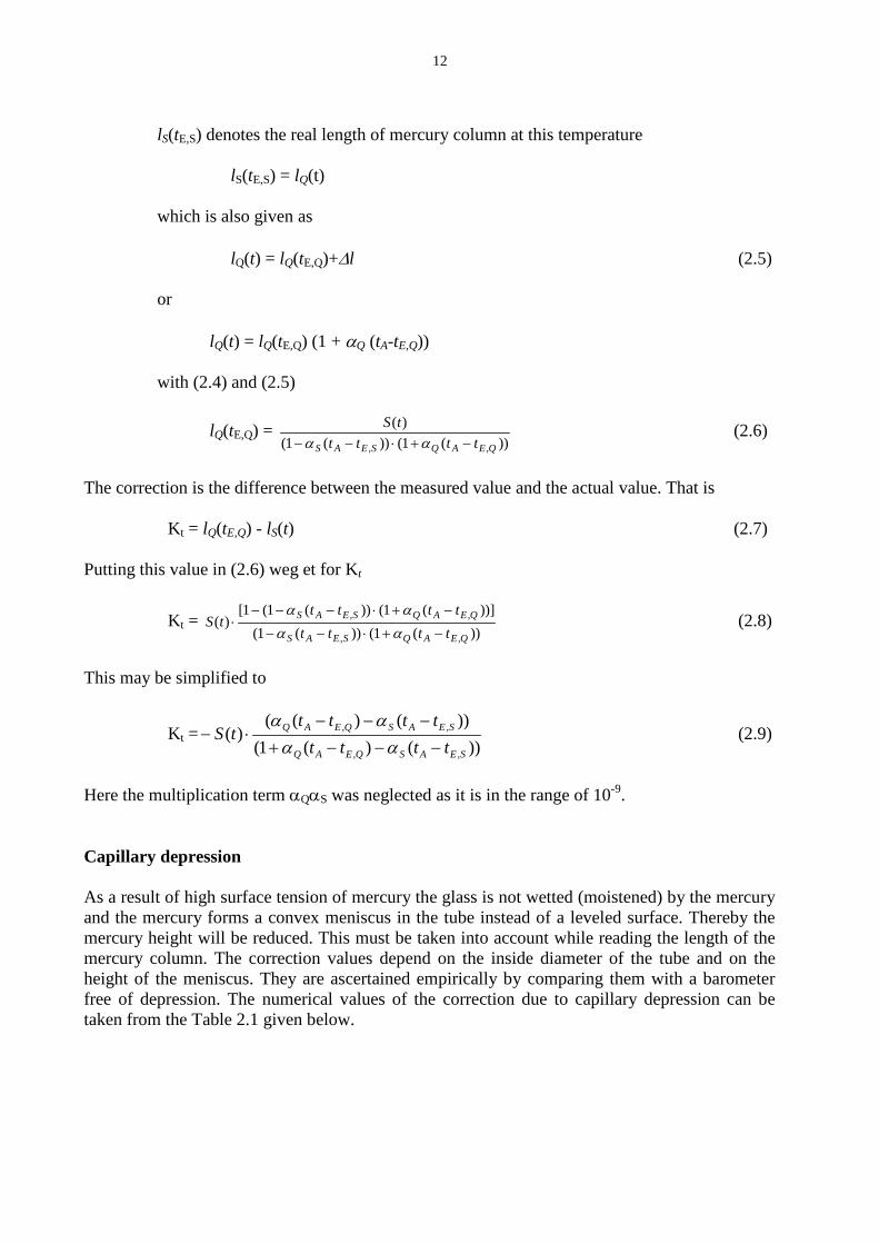
lS(tE,S) denotes the real length of mercury column at this temperature

lS(tE,S) = lQ(t) which is also given as

lQ(t) = lQ(tE,Q)+∆l (2.5) or

lQ(t) = lQ(tE,Q) (1 + αQ (tA-tE,Q)) with (2.4) and (2.5)

lQ(tE,Q) = ))(1())(1(

)(

,, QEAQSEAS tttttS

−+⋅−− αα (2.6)

The correction is the difference between the measured value and the actual value. That is

Kt = lQ(tE,Q) - lS(t) (2.7)

Putting this value in (2.6) weg et for Kt

Kt = ))(1())(1(

))](1())(1(1[)(

,,

,,

QEAQSEAS

QEAQSEAS

tttttttt

tS−+⋅−−

−+⋅−−−⋅

αααα

(2.8)

This may be simplified to

Kt = ))()(1())()((

)(,,

,,

SEASQEAQ

SEASQEAQ

tttttttt

tS−−−+

−−−⋅−

αααα

(2.9)

Here the multiplication term αQαS was neglected as it is in the range of 10-9.

Capillary depression As a result of high surface tension of mercury the glass is not wetted (moistened) by the mercury and the mercury forms a convex meniscus in the tube instead of a leveled surface. Thereby the mercury height will be reduced. This must be taken into account while reading the length of the mercury column. The correction values depend on the inside diameter of the tube and on the height of the meniscus. They are ascertained empirically by comparing them with a barometer free of depression. The numerical values of the correction due to capillary depression can be taken from the Table 2.1 given below.

13

Table 2.1: Correction of the barometric length (mm Hg or mbar) due to capillary depres-sion

Capillary height (for 8 mm tube-ϕ) in mm or mbar 0.4 0.5 0.6 0.7 0.8 2.9 1.0 1.1 1.2 1.3 1.4 Kk (mm Hg) 0.24 0.29 0.35 0.41 0.46 0.51 0.56 0.60 0.64 0.68 0.71 Kk (mbar) 0.24 0.30 0.36 0.41 0.47 0.52 0.57 0.63 0.68 0.73 0.77

Capillary height (for 8 mm tube-ϕ) in mm or mbar 1.5 1.6 1.7 1.8 1.9 2.0 2.1 2.2 2.3 2.4 Kk (mm Hg) 0.74 0.77 0.80 0.82 Kk (mbar) 0.81 0.85 0.89 0.93 0.96 0.99 1.02 1.05 1.07 1.09

The correction values KK given in the table (in mm Hg or mbar) are to be added to the baromet-ric values. Correction of gravity Latitude: The length of the mercury column also depends on the acceleration due to gravity, which chang-es with the geographical latitude and the height above sea level. Therefore, the barometric reading is converted to the normal gravity. At sea level below 45° of latitude the gravitational acceleration amounts to 9.80616 m/s². The normal gravity or the standard value of the gravita-tional acceleration is 9.80665 m/s², which is reached at sea level at approximately 45° 33´ geographical latitude. If p is the pressure measured at any geographical latitude, gN the normal acceleration due to gravity, bN the height of the mercury column at normal acceleration due to gravity, bβ the temperature corrected barometric column and gβ the acceleration due to gravity at any geographical place then it holds at the same atmospheric pressure on different places:

p = ρ ⋅gN⋅ bN=ρ ⋅ gβ ⋅ bβ (2.10)

The correction due to gravity for that place is

Kβ=bN-bβ or also Kβ=

−⋅ 1

ββ b

bb N .

Using (2.10) follows:

Kβ=

−⋅ 1

Ngg

b ββ . (2.11)

The acceleration due to gravity changes with the latitude according to the relation:

gβ= 9.80616 – 0,02586 cos2 β + ....

So, one obtains:

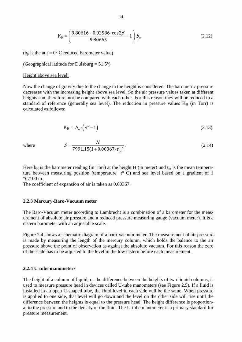
14

Kβ = 9.80616 0.02586 cos2 19.80665

bβ

β − ⋅− ⋅

(2.12)

(bβ is the at t = 0° C reduced barometer value) (Geographical latitude for Duisburg = 51.5°) Height above sea level: Now the change of gravity due to the change in the height is considered. The barometric pressure decreases with the increasing height above sea level. So the air pressure values taken at different heights can, therefore, not be compared with each other. For this reason they will be reduced to a standard of reference (generally sea level). The reduction in pressure values KH (in Torr) is calculated as follows:

KH = ( )1S

Hb e⋅ − (2.13)

where 7991.15(1 0.00367 )m

HSt

=+ ⋅

. (2.14)

Here bH is the barometer reading (in Torr) at the height H (in meter) und tm is the mean tempera-ture between measuring position (temperature t° C) and sea level based on a gradient of 1 °C/100 m. The coefficient of expansion of air is taken as 0.00367.

2.2.3 Mercury-Baro-Vacuum meter The Baro-Vacuum meter according to Lambrecht is a combination of a barometer for the meas-urement of absolute air pressure and a reduced pressure measuring gauge (vacuum meter). It is a cistern barometer with an adjustable scale. Figure 2.4 shows a schematic diagram of a baro-vacuum meter. The measurement of air pressure is made by measuring the length of the mercury column, which holds the balance to the air pressure above the point of observation as against the absolute vacuum. For this reason the zero of the scale has to be adjusted to the level in the low cistern before each measurement. 2.2.4 U-tube manometers The height of a column of liquid, or the difference between the heights of two liquid columns, is used to measure pressure head in devices called U-tube manometers (see Figure 2.5). If a fluid is installed in an open U-shaped tube, the fluid level in each side will be the same. When pressure is applied to one side, that level will go down and the level on the other side will rise until the difference between the heights is equal to the pressure head. The height difference is proportion-al to the pressure and to the density of the fluid. The U-tube manometer is a primary standard for pressure measurement.

15

Differential pressure can be measured by connecting each of the legs to one of the measurement points. Absolute pressure can be measured by evacuating the reference side. A mercury barome-ter is such an absolute pressure measuring manometer indicating atmospheric pressure. In some versions, the two legs of the U are of different diameters. Some types incorporate a large-diameter "well" on one side. In others, one tube is inclined in order to provide better resolution of the reading. But they all operate on the same principle. Because of the many constraints on geometry of installation and observation, and their limited range, manometers are not practical or effective for most pressure measurements. Although many manometers are simply a piece of glass tubing formed into a U shape with a reference scale for measuring heights, there are many variations in terms of size, shape, and material (see Figure 2.5). If the left side is connected to the measurement point, and the right is left open to atmosphere, the manometer will indicate gauge pressure, positive or negative (vacu-um). Any fluid can be used in a manometer. However, mercury is preferred for its high density (13.534 g/cm3) and low vapor pressure. For low pressure differences well above the vapor pressure of water, water is commonly used (and "inches of water" is a common pressure unit). U-tube liquid-column pressure gauges are independent of the type of gas being measured and have a highly linear calibration. They have poor dynamic response. When measuring vacuum, the working liquid may evaporate and contaminate the vacuum if its vapor pressure is too high. When measuring liquid pressure, a loop filled with gas or a light fluid must isolate the liquids to prevent them from mixing. Simple hydrostatic gauges can measure pressures ranging from a few Torr (a few 100 Pa) to a few atmospheres (Approximately 1000000 Pa). One manometer which is extensively used is that according to Bennert shown in Figure 2.6. It consists of a vertical standing U-tube of glass whose one arm is evacuated. The other arm is connected to an inverted U-tube. The lower end of this can be closed with the help of a valve and is connected to the pressure being measured. A scale is brought between the arms (see Figure 2.6) to measure the difference in the levels of the liquid in the two arms. It can be used to meas-ure absolute pressures between 1 and 200 Torr. 2.2.5 Thermal conductivity vacuum meter The thermal conductivity vacuum meter is an indirect device for pressure measurement. General-ly, an increase in the density of a real gas (which also indicates an increase in pressure) increases its ability to conduct heat. In this type of gauge, a wire filament is heated by running current through it. A thermocouple or Resistance Temperature Detector (RTD) can then be used to measure the temperature of the filament. This temperature is dependent on the rate at which the filament loses heat to the surrounding gas, and therefore on the thermal conductivity. A common variant is the Pirani gauge which uses a single platinum filament as both the heated element and RTD. The operating principle of this type of instruments is that the heat loss by conduction and convection from a heated resistance wire depends on the pressure of the gas surrounding the wire. These gauges are accurate from 10 Torr to 10−3 Torr, but they are sensitive to the chemical composition of the gases being measured. Under high vacuum the heat flow due to gas convection does not depend upon pressure (see Figure 2.7) and so these gauges are not useful. For higher pressures the thermal conductance changes very little with pressure.

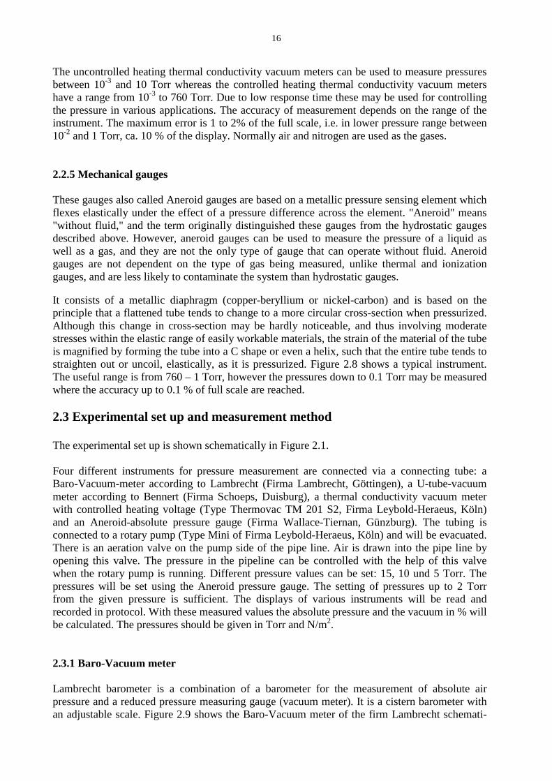
16

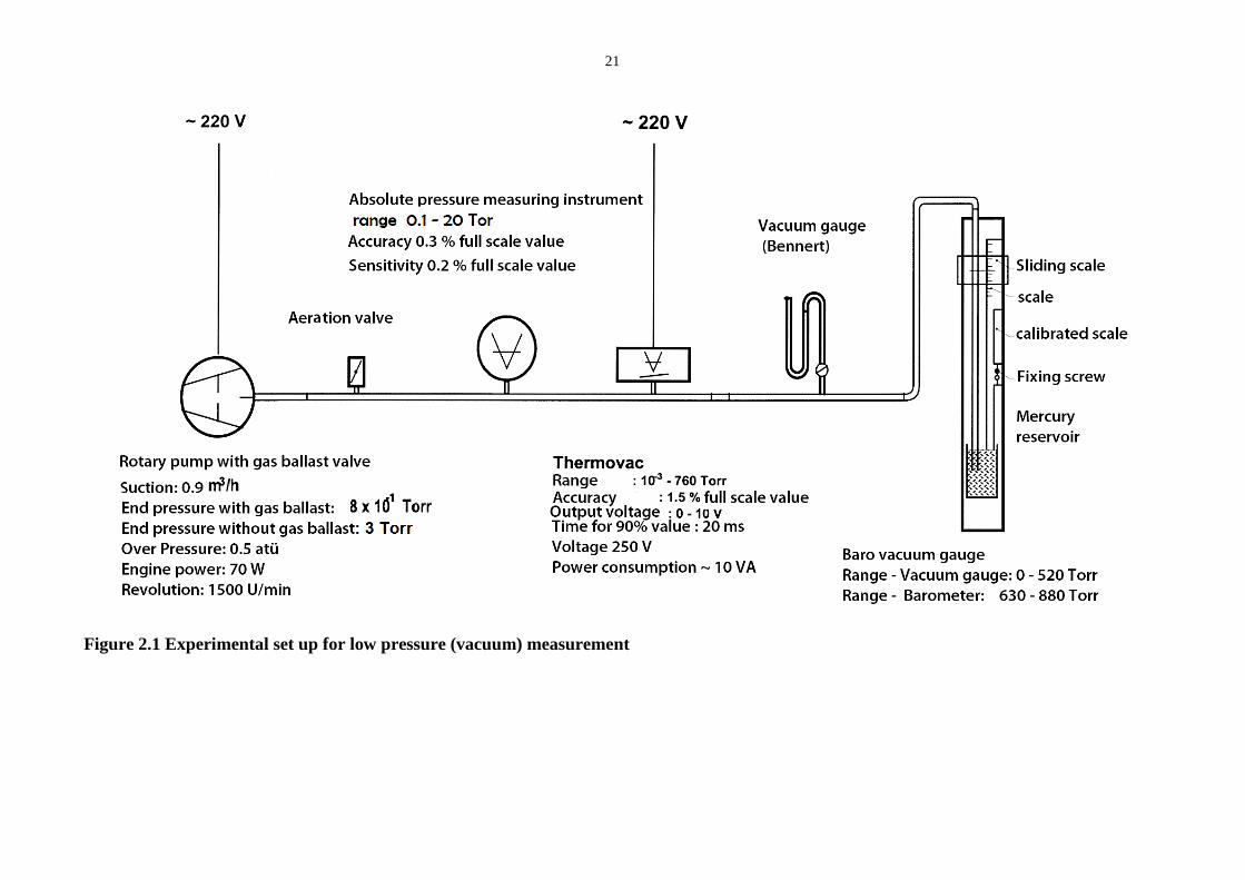
The uncontrolled heating thermal conductivity vacuum meters can be used to measure pressures between 10-3 and 10 Torr whereas the controlled heating thermal conductivity vacuum meters have a range from 10-3 to 760 Torr. Due to low response time these may be used for controlling the pressure in various applications. The accuracy of measurement depends on the range of the instrument. The maximum error is 1 to 2% of the full scale, i.e. in lower pressure range between 10-2 and 1 Torr, ca. 10 % of the display. Normally air and nitrogen are used as the gases. 2.2.5 Mechanical gauges These gauges also called Aneroid gauges are based on a metallic pressure sensing element which flexes elastically under the effect of a pressure difference across the element. "Aneroid" means "without fluid," and the term originally distinguished these gauges from the hydrostatic gauges described above. However, aneroid gauges can be used to measure the pressure of a liquid as well as a gas, and they are not the only type of gauge that can operate without fluid. Aneroid gauges are not dependent on the type of gas being measured, unlike thermal and ionization gauges, and are less likely to contaminate the system than hydrostatic gauges. It consists of a metallic diaphragm (copper-beryllium or nickel-carbon) and is based on the principle that a flattened tube tends to change to a more circular cross-section when pressurized. Although this change in cross-section may be hardly noticeable, and thus involving moderate stresses within the elastic range of easily workable materials, the strain of the material of the tube is magnified by forming the tube into a C shape or even a helix, such that the entire tube tends to straighten out or uncoil, elastically, as it is pressurized. Figure 2.8 shows a typical instrument. The useful range is from 760 – 1 Torr, however the pressures down to 0.1 Torr may be measured where the accuracy up to 0.1 % of full scale are reached. 2.3 Experimental set up and measurement method The experimental set up is shown schematically in Figure 2.1. Four different instruments for pressure measurement are connected via a connecting tube: a Baro-Vacuum-meter according to Lambrecht (Firma Lambrecht, Göttingen), a U-tube-vacuum meter according to Bennert (Firma Schoeps, Duisburg), a thermal conductivity vacuum meter with controlled heating voltage (Type Thermovac TM 201 S2, Firma Leybold-Heraeus, Köln) and an Aneroid-absolute pressure gauge (Firma Wallace-Tiernan, Günzburg). The tubing is connected to a rotary pump (Type Mini of Firma Leybold-Heraeus, Köln) and will be evacuated. There is an aeration valve on the pump side of the pipe line. Air is drawn into the pipe line by opening this valve. The pressure in the pipeline can be controlled with the help of this valve when the rotary pump is running. Different pressure values can be set: 15, 10 und 5 Torr. The pressures will be set using the Aneroid pressure gauge. The setting of pressures up to 2 Torr from the given pressure is sufficient. The displays of various instruments will be read and recorded in protocol. With these measured values the absolute pressure and the vacuum in % will be calculated. The pressures should be given in Torr and N/m2. 2.3.1 Baro-Vacuum meter Lambrecht barometer is a combination of a barometer for the measurement of absolute air pressure and a reduced pressure measuring gauge (vacuum meter). It is a cistern barometer with an adjustable scale. Figure 2.9 shows the Baro-Vacuum meter of the firm Lambrecht schemati-

17

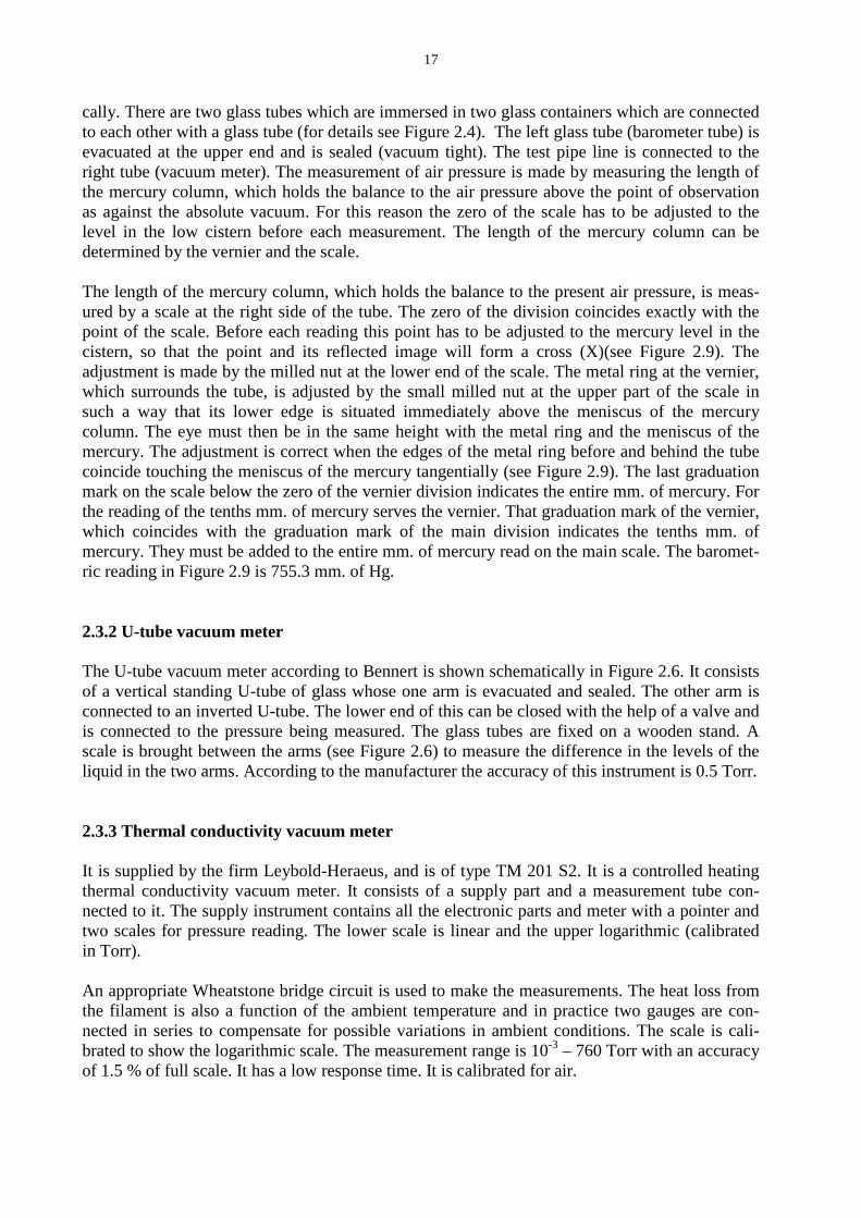
cally. There are two glass tubes which are immersed in two glass containers which are connected to each other with a glass tube (for details see Figure 2.4). The left glass tube (barometer tube) is evacuated at the upper end and is sealed (vacuum tight). The test pipe line is connected to the right tube (vacuum meter). The measurement of air pressure is made by measuring the length of the mercury column, which holds the balance to the air pressure above the point of observation as against the absolute vacuum. For this reason the zero of the scale has to be adjusted to the level in the low cistern before each measurement. The length of the mercury column can be determined by the vernier and the scale. The length of the mercury column, which holds the balance to the present air pressure, is meas-ured by a scale at the right side of the tube. The zero of the division coincides exactly with the point of the scale. Before each reading this point has to be adjusted to the mercury level in the cistern, so that the point and its reflected image will form a cross (X)(see Figure 2.9). The adjustment is made by the milled nut at the lower end of the scale. The metal ring at the vernier, which surrounds the tube, is adjusted by the small milled nut at the upper part of the scale in such a way that its lower edge is situated immediately above the meniscus of the mercury column. The eye must then be in the same height with the metal ring and the meniscus of the mercury. The adjustment is correct when the edges of the metal ring before and behind the tube coincide touching the meniscus of the mercury tangentially (see Figure 2.9). The last graduation mark on the scale below the zero of the vernier division indicates the entire mm. of mercury. For the reading of the tenths mm. of mercury serves the vernier. That graduation mark of the vernier, which coincides with the graduation mark of the main division indicates the tenths mm. of mercury. They must be added to the entire mm. of mercury read on the main scale. The baromet-ric reading in Figure 2.9 is 755.3 mm. of Hg. 2.3.2 U-tube vacuum meter The U-tube vacuum meter according to Bennert is shown schematically in Figure 2.6. It consists of a vertical standing U-tube of glass whose one arm is evacuated and sealed. The other arm is connected to an inverted U-tube. The lower end of this can be closed with the help of a valve and is connected to the pressure being measured. The glass tubes are fixed on a wooden stand. A scale is brought between the arms (see Figure 2.6) to measure the difference in the levels of the liquid in the two arms. According to the manufacturer the accuracy of this instrument is 0.5 Torr. 2.3.3 Thermal conductivity vacuum meter It is supplied by the firm Leybold-Heraeus, and is of type TM 201 S2. It is a controlled heating thermal conductivity vacuum meter. It consists of a supply part and a measurement tube con-nected to it. The supply instrument contains all the electronic parts and meter with a pointer and two scales for pressure reading. The lower scale is linear and the upper logarithmic (calibrated in Torr). An appropriate Wheatstone bridge circuit is used to make the measurements. The heat loss from the filament is also a function of the ambient temperature and in practice two gauges are con-nected in series to compensate for possible variations in ambient conditions. The scale is cali-brated to show the logarithmic scale. The measurement range is 10-3 – 760 Torr with an accuracy of 1.5 % of full scale. It has a low response time. It is calibrated for air.

18

2.3.4 Aneroid absolute pressure gauge A precise instrument from the firm Wallace and Tiernan is used. The measuring element is an evacuated Cu-Beryllium-C-capsule. It is a robust instrument with good temperature stability and has a very low response time. The accuracy of this instrument is 0.3 % of the full scale value.

2.4 Experimental Method

1. Turn on the thermal conductivity (Pirani) vacuum gauge and the vacuum pump.

2. Adjust the zero point of barometer scale (see Figure). For the adjustment method see

“Mercury Baro- Vacuum gauge, 6. Measurement”.

3. Record the barometer reading in the protocol.

4. Open the stop valve at the upper end of the vacuum meter and the U-tube manometer.

5. Close the regulating (loop) valve.

6. Observe the manometer till the pressure drops to 15 Torr.

7. Open the regulating valve slowly so that the manometer readings given in the protocol

are attained (say 15 Torr). Wait until the reading is constant (± 2 Torr).

8. Adjust the left tube of the barometer as described under step 2 to the new column

height.

9. Read the height of mercury column in vacuum meter tube (right tube) after the ad-

justment that the edges of metal ring before and behind the tube coincide touching the

meniscus of the mercury tangentially.

10. Record the reading in the protocol.

11. Check the pressure at the vacuum meter. The change should not be larger than ± 0.1

Torr. Otherwise regulate the pressure again and take new reading.

12. Read the pressure gauge and record the reading in the protocol.

13. Adjust the zero point of mirror scale of U-tube vacuum meter up to the mercury col-

umn height in the left side of the tube.

14. Check the adjusted pressure at the manometer. If necessary regulate the pressure with

the help of regulating valve.

15. Read the difference of mercury column height on the two sides.

16. Read the conductivity vacuum gauge and record the reading in the protocol.

17. Now adjust the pressure to another value (10 Torr).

18. Wait till the value is constant.

19. Repeat the steps 4-16.

20. Now adjust the pressure to 5 Torr and repeat the steps 4-16.

19

21. Open the regulating valve slowly until the mercury height in the U-tube vacuum me-

ter attains highest value then open the valve completely.

22. Shut off the vacuum pump and conductivity meter gauge.

23. Close the valve at U-tube vacuum meter and Baro vacuum meter.

24. Evaluate the barometer readings taking into account all the corrections discussed in

section 2.2.2. The corrected barometer reading in Torr is given as:

KHttO KKKKbb ++++= β

bt = Barometer reading Kt = Temperature correction Kß = Gravity correction, latitude KH = Gravity correction, height KK = Capillary height correction

The correction term for the capillary height will be taken from table 2.1 and all other

correction factors will be calculated by the formula given in section 2.2.2. The room

temperature should be taken from the Lambrecht barometer reading. The latitude for

Duisburg is to be taken as 51.5 ° and the height (including the place of measurement)

above sea level as 40 m.

25. Draw graph showing the % deviation of values measured with different instruments

from the value of the Aneroid pressure gauge (see section 2.3).

26. Calculate the vacuum in % from the values of Baro vacuum meter.

27. Give values in Pa and bar.

20

Protocol-2

Date: Matr.-No.: Time: Name: Experiment 2: Measurement of low pressure (vacuum) Temperature:

Barometer

reading

[mm Hg]

Capillary

height

[mm Hg]

Temperatur correction

[mm Hg]

Gravity

Correction

[mm Hg]

Height

Correction

[mm Hg]

Capillary

Correction

[mm Hg]

Actual re-duced baro-meter reading [mm Hg]

Aneroid

Vacuum meter

Baro

Vacuum meter

[Torr]

U-tube

manometer

[Torr]

Thermovac

Thermal con-ductivity

Vacuum meter

[Torr]

Vacuum

(%)

p

[Pascal]

actual [Torr]

read

[Torr]

15 10

5

21

Figure 2.1 Experimental set up for low pressure (vacuum) measurement

22

Figure 2.2 Useful ranges for different pressure measuring instruments

23

Figure 2.3 Various pressure reference points

Figure 2.4 Schematic representation of a baro vacuum meter

24

Figure 2.5 Different U-tube configurations for pressure measurements

25

Figure 2.6 U-tube vacuum meter (Bennert)

26

Figure 2.7 Dependence of heat flux on gas pressure for a heated wire (radius r1) in a tube (radius r2)

Figure 2.8 Schematic diagram of an Aneroid gauge

27

Figure 2.9 Schematic diagram of a baro-vacuum meter (Lambrecht)