UNIVERSITY OF CALGARY

Constructing and Tabulating Dihedral Function Fields

by

Colin Weir

A THESIS

SUBMITTED TO THE FACULTY OF GRADUATE STUDIES

IN PARTIAL FULFILLMENT OF THE REQUIREMENTS FOR THE

DEGREE OF DOCTOR OF PHILOSOPHY

DEPARTMENT OF MATHEMATICS AND STATISTICS

CALGARY, ALBERTA

AUGUST, 2013

c© Colin Weir 2013

Abstract

We present and implement algorithms for constructing and tabulating odd prime

degree ` dihedral extensions of a rational function field k0(x), where k0 is a perfect field

with characteristic not dividing 2`. We begin with a class field theoretic construction

algorithm when k0 is a finite field. We also describe modifications to this algorithm

to improve the run time of its implementation.

Subsequently, we introduce a Kummer theoretic algorithm for constructing dihe-

dral function fields with prescribed ramification and fixed quadratic resolvent field,

when k0 is a perfect field and not necessarily finite. We give a detailed description of

this Kummer theoretic approach when k0, or a quadratic extension thereof, contains

the `-th roots of unity. Avoiding the case when k0 is infinite and the quadratic resol-

vent field is a constant field extension of k0(x), we show that our Kummer theoretic

algorithm constructs all degree ` dihedral extensions of k0(x) with prescribed rami-

fication. This algorithm is based on the proof of our main theorem, which gives an

exact count of such fields.

When k0 is a finite field, we implement and experimentally compare the run times

of the class field theoretic and Kummer theoretic construction algorithms. We find

that the Kummer theoretic approach performs better in all cases, and hence we use

it later in our tabulation method.

Lastly, utilizing the automorphism group of Fq(x), we present a tabulation algo-

rithm to construct all degree ` dihedral extensions of Fq(x) up to a given discrimi-

nant bound, and we present tabulation data. This data is then compared to known

ii

asymptotic predictions, and we find that these estimates over-count the number of

such fields. We also give a formula for the number of degree ` dihedral extensions of

Fq(x) when q ≡ ±1 mod 2`, with discriminant divisors of minimum possible degree.

iii

Table of Contents

Abstract ii

Table of Contents iv

1 Introduction 11.1 Structural Overview . . . . . . . . . . . . . . . . . . . . . . . . . . . 6

2 Background and Preliminary Results 132.1 Function Fields . . . . . . . . . . . . . . . . . . . . . . . . . . . . . . 13

2.1.1 Algebraic Function Fields . . . . . . . . . . . . . . . . . . . . 142.1.2 Places . . . . . . . . . . . . . . . . . . . . . . . . . . . . . . . 152.1.3 Extensions of Function Fields . . . . . . . . . . . . . . . . . . 182.1.4 Divisors, Genus and Different . . . . . . . . . . . . . . . . . . 20

2.2 Galois Representations and L-functions . . . . . . . . . . . . . . . . . 262.2.1 Galois Theory of Function Fields . . . . . . . . . . . . . . . . 262.2.2 Representation Theory . . . . . . . . . . . . . . . . . . . . . . 292.2.3 L-functions . . . . . . . . . . . . . . . . . . . . . . . . . . . . 34

2.3 Dihedral Function Fields . . . . . . . . . . . . . . . . . . . . . . . . . 36

3 Construction of Dihedral Function Fields via Class Field Theory 423.1 Class Fields of Function Fields . . . . . . . . . . . . . . . . . . . . . . 433.2 Class Field Theoretic Construction Algorithms . . . . . . . . . . . . . 46

4 Kummer Theoretic Approach with `-th Roots of Unity 584.1 Constructing and Counting Dihedral Function Fields . . . . . . . . . 59

4.1.1 Kummer Theory . . . . . . . . . . . . . . . . . . . . . . . . . 604.1.2 Virtual Unit Decomposition . . . . . . . . . . . . . . . . . . . 654.1.3 The Number of D` Function Fields . . . . . . . . . . . . . . . 704.1.4 Defining equations . . . . . . . . . . . . . . . . . . . . . . . . 73

4.2 Construction Algorithms . . . . . . . . . . . . . . . . . . . . . . . . . 74

5 Kummer Theoretic Approach without `-th Roots of Unity 845.1 Construction with Quadratic Resolvent K2 = K0(ζ`) . . . . . . . . . . 855.2 Construction with Quadratic Resolvent K2 when K2/K0 is geometric 925.3 Construction when K2/K0 is geometric and [k0(ζ`) : k0] = 2 . . . . . . 965.4 Construction Algorithms when [k0(ζ`) : k0] = 2 . . . . . . . . . . . . . 99

iv

6 Numerical Results and Tabulation Techniques 1066.1 Tabulation Method . . . . . . . . . . . . . . . . . . . . . . . . . . . . 1076.2 Implementations and Numerical Results . . . . . . . . . . . . . . . . 111

6.2.1 Asymptotic Comparison when ` = 3 . . . . . . . . . . . . . . . 1136.2.2 Explicit Formulas for B = 2(`− 1) . . . . . . . . . . . . . . . 116

6.3 Tables of Numerical Data . . . . . . . . . . . . . . . . . . . . . . . . 120

7 Conclusions 125

Bibliography 132

v

1

Chapter 1

Introduction

Two important problems in algebraic and algorithmic number theory are the con-

struction of global fields of a fixed discriminant or prescribed ramification – with its

curve analogue of constructing Galois covers of fixed genus – and the tabulation of

global fields with a certain Galois group up to some discriminant or genus bound. The

latter problem goes hand in hand with asymptotic estimates for the number of such

fields; for example, estimates for cubic number fields were first given in [15] and for

quartics in [3]. There is a sizable body of literature on construction, tabulation, and

asymptotic counts of number fields; a rather comprehensive survey of known results

can be found in [9], and extensive tables of data are available at [26].

Far less is known in the function field setting; only the asymptotic counts for

cubic [14] and abelian [43] extensions have been proved. However, there is a general

program described by Venkatesh and Ellenberg [40] for formulating these asymptotic

estimates for both number fields and function fields. In particular, they point out

the “alarming gap between theory and experiment” in asymptotic predictions for

number fields. In the case of cubic number fields, this inconsistency led Roberts

[29] to conjecture the secondary term in the theorem of Davenport and Heilbronn

in [15]. His conjecture was later proved independently by Bhargava, Shankar, and

Tsimerman [4] and by Taniguchi and Thorne [39]. In the function field setting,

2

however, there is practically no experimental data to potentially identify a similar such

gap. In fact, the only known algorithms for constructing non-abelian function fields

are those which construct non-Galois cubic fields with squarefree discriminant [25].

Recently although, Pohst [28] showed how to construct all non-Galois cubic extensions

of Fq(x) with a given discriminant, which also leads to such an algorithm (though

no description of an implementation is provided in [28]). In fact, Pohst’s method is

a special case of the class field theoretic approach that we will present. Tabulation

methods for certain classes of cubic function fields with squarefree discriminants can

be found in [31], [33] and [32], though neither can provide complete lists of cubic

function fields in general.

This thesis represents the next steps in function field construction and tabulation.

We present, implement, and compare new algorithms for constructing all odd prime

degree dihedral function fields with prescribed ramification (which includes all non-

Galois cubics) over finite fields in all characteristics greater than 3, and over infinite

perfect fields under some restrictions. This provides the first example of a method to

construct function fields over infinite constant fields with a fixed non-abelian Galois

group and given ramification. Via these method we are able to provide the first

complete tables of function fields over finite fields whose discriminant divisors have

degree below a fixed bound. In particular, only now can the asymptotic estimates

for cubic function fields be truly compared to the actual number of cubic fields in

characteristics greater than 3. Moreover, via Kummer theory, we obtain a new and

fruitful understanding of dihedral function fields. With this view point, we obtain

new explicit formulas for the number of dihedral function fields in several cases,

generalizing the work of Howe in [42].

3

Many of the contributions of this thesis are inspired by the work of Cohen [8, 11]

in the number field setting, and based upon my work that first appeared in [42].

Let ` be an odd prime. In [42] we presented a method for constructing all degree `

extensions of Fq(x) with prescribed ramification and with Galois group isomorphic

to the dihedral group of order 2`, when q ≡ 1 mod 2`. Here, and going forward, we

make the common abuse of language by saying that a field has Galois group G when

we are in fact referring to the Galois group of its Galois closure.

In [42] we used a Kummer-theoretic approach inspired by the methods of Cohen

[8, Ch 5], [11] for number fields. This construction method can be converted into

a tabulation algorithm in the usual manner via iteration. However, in [42] we ex-

plained how to use the automorphism group PGL(2, q) of Fq(x) to effect significant

speed-ups in this case. We note that this technique is unique to the function field

setting and cannot be utilized in the number field scenario, as there are no nontrivial

automorphisms on the rational numbers. Exploiting Fq(x)-automorphisms reduces

the number of constructions by a factor of order q3 compared to the naıve approach.

We presented our improved tabulation procedure along with numerical data obtained

from an implementation in Magma [5]. It is important to note that in the special

case ` = 3, our algorithm generates complete tables of non-Galois cubic function fields

over Fq(x) up to a given discriminant bound when q ≡ 1 mod 3.

In this thesis we present two general methods for constructing degree ` dihedral

function fields. First, we explore a class field theoretic technique for constructing

dihedral function fields over finite fields with characteristic different from 2 and `.

We then show how to improve this algorithm, making it practical for implementation

purposes. We note that this method specializes to the one presented in [28] when

4

` = 3. We also note that we developed our algorithm before the publication of [28]

and were unaware of Pohst’s work at the time.

Second, we present the Kummer theoretic approach of [42], but generalized to a

wider class of function fields. We extend this approach to construct degree ` dihedral

function fields over an arbitrary perfect field k0 of characteristic not dividing 2`,

when k0, or a quadratic extension thereof, contains the `-th roots of unity. When k0

is a finite field Fq, we thus obtain algorithms for constructing all dihedral function

fields with prescribed ramification when q ≡ ±1 mod 2`. Notice that when ` =

3, this now allows us to construct (and later tabulate) non-Galois cubic function

fields over finite fields of characteristic greater than 3. When k0 is not finite, but

perfect and of characteristic not dividing 2`, we obtain a method for constructing all

dihedral function fields with prescribed ramification whose quadratic resolvent field

is not a constant field extension of k0(x). Hence, eventually we make the following

assumption:

Assumption: COEFF (C onstants are Only Extended over F inite F ields). When K2

is a quadratic constant field extension of a rational function field K0, we assume that

the constant field k0 of K0 is a finite field. When K2/K0 is a geometric field extension,

we do not assume that k0 is finite, only that it is perfect. In both cases we assume

that char(k0) - 2`.

The reasons for this restriction are quite natural. All extensions of finite fields

are cyclic and thus not dihedral. However, when k0 is a number field for example,

there are infinitely many degree ` dihedral extensions of k0 and hence infinitely many

unramified dihedral extensions of k0(x). The methods to construct and tabulate

such extensions are number field theoretic and beyond the scope of this thesis (see

5

[8, Ch 8,9] and [11] for known methods). Consequently, we will eventually need to

invoke Assumption COEFF to avoid this case. However, given a discriminant divisor

∆ that is not a multiple of ` − 1, our algorithms construct all geometric degree `

dihedral function fields with perfect constant field k0 and discriminant ∆ when the

characteristic of k0 does not divide 2`. Therefore, this thesis contains the first known

algorithm for constructing all geometric function fields over an infinite constant field

with a fixed non-abelian Galois group and prescribed ramification.

When the constant field k0 is a finite field Fq, we implement the class field the-

oretic and Kummer theoretic approaches in Magma [5], and compare the two for

several values ` and q where q ≡ ±1 mod 2`. For the case ` = 3, to the best of my

knowledge, this is the first implementation and profiling of the class field theoretic

algorithm discussed in [28]. However, we find that our Kummer theoretic algorithm

is multiple times faster than the class field theoretic method in all cases considered,

and considerably faster still when q ≡ −1 mod 2`. Hence, we later use the Kummer

theoretic method in our tabulation algorithms.

To tabulate dihedral fields, we use the technique I first developed in [42]. In this

thesis, we show how to use the automorphism group PGL(2, q) of Fq(x) to improve

tabulation over an arbitrary finite field. We present our improved tabulation proce-

dure and the numerical data obtained from an implementation in Magma [5]. We

then compare this data to the asymptotic formula of [14] when ` = 3. This represents

the first true comparison of this formula to complete counts of cubic function fields

over Fq when q ≡ −1 mod 3 (the case q ≡ 1 mod 3 was originally presented in [42]).

As in the number field setting, we find considerable “gaps” between the asymptotic

predictions and the actual number of cubic function fields, regardless of the character-

6

istic. Moreover, like the number field setting, the asymptotic formulas overestimate

the actual number of cubic fields.

Lastly, we provide an explicit formula for the number of degree ` dihedral function

fields over a finite field whose discriminants divisor have smallest possible degree.

This formula is originally due to Howe [42] for the case q ≡ 1 mod 2`, and here we

extend it to the case when q ≡ −1 mod 2`. An interesting consequence of these two

formulas is that the total number of index ` subgroups of class groups of genus 1

quadratic extensions of Fq(x) is a function of ` and q which does not vary with the

presence of `-th roots of unity in Fq. We find this especially interesting because the

expected number of index ` subgroups in the class group of any one of these extensions

depends on the presence of `-th roots of unity in Fq. These and other consequences

are discussed further in the conclusions (Chapter 7).

In summary, we present, implement, and compare new algorithms for construct-

ing all dihedral function fields of odd prime degree with a given discriminant divisor.

When the constant field is infinite, this yields the first method to construct func-

tion fields with a fixed non-abelian Galois group and given ramification. New and

complete tables of function fields over finite fields are produced and compared to the

known asymptotic estimates. Moreover, via Kummer theory, we present an in-depth

approach to dihedral function fields, giving rise to new explicit formulas for counting

the number of these fields in several cases.

1.1 Structural Overview

Throughout this thesis we make a strong effort towards notational consistency and

hence use several conventions. For example, K will always denote an arbitrary func-

7

tion field with constant field k, while K ′ will denote an extension of K. K0 is always

a rational function field with constant field k0 and transcendental x. We use Ki to

denote a degree i extension of K0, where K2 is obtained by adjoining y or z. Note that

we nearly always assume that char(k0) - 2`, where ` is an odd prime. The letter T is

reserved for the transcendental of a polynomial ring. Furthermore, general groups are

represented with the calligraphy font (G, H for example), and their elements are al-

ways Greek letters (usually %, τ, σ, γ); this includes Galois groups and automorphism

groups. However, α, β, κ, θ are reserved for elements of a function field, with κ typi-

cally in K0, and θ typically a root of T `−α. Capital Greek letters are used for maps.

Divisors of K are denoted with capital letters such as D,E, while divisors of K ′ are

denoted with D′, E ′. Constants, including elements of k0, are represented with lower

case letters. The remaining notation is introduced as needed.

In Chapter 2, we present a range of material required to understand and describe

dihedral function fields. In the first section, we describe function fields and their

extensions, places and their valuations. We then we discuss divisors and Riemann-

Roch spaces amoung other topics. This allows us to present definitions for the genus,

different and discriminant divisor of a function field, and state the Riemann-Hurwitz

genus formula. With this introductory material in hand, the main goal of the rest of

this chapter is to introduce the subject matter required to prove Theorem 2.3.2; an

explicit formula for the discriminant divisor of a dihedral function field.

In Section 2.2, we recall basic Galois theory and describe the action of the Galois

group of a function field on its various structures. This section also contains the

definitions of interia and decomposition groups which will become useful later on for

presenting Artin L-functions.

8

As Artin L-functions are associated to representations, Subsection 2.2.2 presents

a basic introduction to finite representation theory. The definition of a finite Galois

representation is given along with that of its associated character. Moreover, we

discuss the representations of the group D`, the dihedral group with 2` elements.

It is here that we find a linear relationship between the characters of the induced

representations of subgroups of D`.

Subsection 2.2.3 begins with an introduction to zeta function of an algebraic func-

tion field, which then leads to an introduction to Artin L-functions. At this point

we see that the Artin L-function of an induced representation is the zeta function of

its fixed field, and that the Artin L-function of the sum of two representations if the

product of the L-functions of these representations. This is a key componenent of

the proof of Theorem 2.3.2, which is finally provided in the following section. The

chapter concludes with a general description of how we intend to construct dihedral

function fields, namely by constructing cyclic degree ` extensions of quadratic fields,

such that the resulting field is dihedral and has the correct discriminant divisor.

As we wish to construct cyclic extensions of quadratic fields, we proceed to study

class field theory. In Chapter 3 we begin with a brief introduction to the main results

of class field theory of function fields. In Section 3.2 we see how to use class field theory

to construct all dihedral function fields over a finite field with a given discriminant

divisor. In particular, we show that one can construct cyclic extensions of quadratic

fields by considering index ` subgroups of ray class groups. Moreover, we discuss how

all dihedral function fields over finite fields can be constructed in this way. These

ideas are first presented in Algorithm 3.1, and to the best of my knowledge are new

results for ` > 3. We then prove two propositions that allow us to refine Algorithm 3.1

9

into the more practical version described by Algorithm 3.2. Much later in the thesis,

in Chapter 6, we discuss the implementation of Algorithm 3.2 and show that, while

it is widely applicable, it computes dihedral fields much slower than the Kummer

theoretic algorithms presented in the next two chapters.

In Chapter 4, we present an alternative to Algorithm 3.1 when the underlying

rational function field contains the `-th roots of unity. This chapter is based upon

my work that first appeared in [42], though generalized to prefect constant fields with

`-th roots of untiy under Assumption COEFF. The material of [42] was edited by

Everett Howe who made several additinos to the proofs and notation. In particular, in

Subsection 4.1.4, we present his method for producing defining equations for dihedral

function fields, instead of the one I originally proposed. The remainder of this chapter,

however, is primarily my own work.

The construction method of Chapter 4 stems from Kummer theory as presented

in Section 4.1.1. Kummer theory states that if a function field K contains the `-

th roots of unity, then every cyclic degree ` extension K ′/K is radical, i.e. K ′ =

K(√α) for some α ∈ K. The remainder of this chapter is primarily dedicated to

constructing elements α in a quadratic field such that the resulting Kummer extension

is dihedral with the appropriate discriminant divisor. To that end, in Subsection 4.1.2

we introduce the theory of (`-)virtual units for function fields. This is based upon the

ideas of Cohen in the number field setting [11]. Of note is the fact that we present

the theory of virtual units independent of the presence of roots of unity. This will

become especially useful in the following chapter.

In Subsection 4.1.3, we give a constructive proof of the main result of Chapter 4; an

exact count of the number of dihedral degree ` extensions of K0 with a given quadratic

10

resolvent field K2 and discriminant divisor ∆. This naturally leads to Algorithm 4.1

in Section 4.2 for constructing degree ` dihedral function fields. Here make use of

Howe’s formula for defining equations [42] which we present in Subsection 4.1.4.

In Chapter 5, we present original work to construct dihedral function fields via

Kummer theory when k0 does not contain the `-th roots of unity. First, in Section 5.1,

we consider the case when the quadratic resolvent field K2 = K0(ζ`). Upon making

Assuption COEFF, we restrict to the case that k0 is a finite field. We then apply our

Kummer theoretic approach to this case and present Algorithm 5.1 to construct all

degree ` dihedral function fields with a given discriminant divisor.

In the following section we consider the situation when the quadratic resolvent

field K2 is a geometric extension of K0. In this case we adjoin the roots of unity to

K2 and apply our Kummer theoretic methods of Chapter 4 to K2(ζ`). This results

in Algorithm 5.2. The inefficiencies of this generic method motivates our subsequent

restriction to the case [k0(ζ`) : k0] = 2. While this may seem rather restrictive, when

` = 3, this still allows us to construct all non-Galois cubic function fields over finite

fields with characteristic greater than 3, and prescribed ramification.

In Section 5.3, we perform a detailed analysis of the case that K2/K0 is a geometric

extension and [k0(ζ`) : k0] = 2. We show that to apply our Kummer theoretic

construction of dihedral function fields, one does not need to perform calculations in

the quartic field K2(ζ`) but rather in a subfield, namely the quadratic twist of K2.

Indeed, to construct all degree ` dihedral function fields with a given discriminant

divisor ∆ in this case, one need only apply Algorithm 4.1 with input `, ∆, and the

twist of K2. It is this result – that one need only perform calculations in a quadratic

extension of K0 – that leads to significant improvements over the class field theoretic

11

approach in this case. The details of this new method are discussed in Section 5.4,

and presented in Algorithm 5.3.

In Chapter 6 we discuss our findings from tabulating dihedral function fields over

finite fields whose discriminant divisors have degree bounded by B. The general

technique we use for tabulation is my own work originally presented in [42]. Here, we

also compare the implementations of our class field theoretic and Kummer theoretic

construction algorithms for various values of ` and q when q ≡ ±1 mod 2`. In all cases

we considered, the Kummer theoretic approach constructs dihedral fields significantly

faster than the algorithm involving class field theory. The data from our comparison

can be found in Table 6.1, where we also include the ratio of the time it took each

these algorithms to perform the various constructions. This speed-up justifies our use

of the Kummer theoretic algorithms during tabulation.

In Section 6.1, we introduce how to use the automorphism group of K0 to tabulate

function fields more efficiently than the naıve method of iteration. We implement this

approach and summarize our findings for various values of q, `, and B. The data from

our findings is presented in Tables 6.2 and 6.3. In these tables we also record the

approximate improvement factor of our method over the standard method of iteration

with utilizing the automorphism group. In all cases considered our technique is several

times faster than the naıve approach.

With this tabulation data in hand, in Subsection 6.2.1 we compare our data count-

ing cubic function fields to the asymptotic predictions of [14]. We note that there are

no known explicit asymptotic formulas for degree ` dihedral function fields with ` > 3.

We present the results of this comparison when ` = 3 in Table 6.4. As in the number

field setting, we find that the asymptotic estimates over-count the actual number of

12

cubic function fields, resulting in a similar “gap between theory and experiment”, as

pointed out in the number field scenario by Ellenberg and Venkatesh [40].

When q ≡ 1 mod `, Everett Howe in [42] proves an explicit formula for the number

of degree ` dihedral function fields over a finite field Fq whose discriminant divisors

have the smallest possible degree. In Subsection 6.2.2, we present that result and

extend it to the case that q ≡ −1 mod `. We find that the two formulas for these

cases are nearly identical; the only difference being when the quadratic resolvent field

is a constant field extensions. This leads to some interesting conclusions regarding

the `-ranks of genus 1 quadratic function fields. These and other conclusions are

discussed further in Chapter 7.

13

Chapter 2

Background and Preliminary

Results

2.1 Function Fields

The goal of this section is to recall basic and relevant facts about algebraic function

fields. We begin with the fundamental theory of algebraic function fields by describing

places, divisors, discriminants, and the genera of function fields and their extensions.

This is followed by recalling basic representation theory, leading to an introduction

of Galois representations and their corresponding L-functions. With this material in

mind, we conclude with some preliminary results on dihedral function fields.

Throughout, k will denote an arbitrary perfect field, and k[x] the univariate poly-

nomial ring over a field k. Also, q will be a power of a prime p, and Fq will denote

the finite field with q elements. While much of the theory of function fields will be

described over any field, we will typically be concerned with function fields over finite

fields.

14

2.1.1 Algebraic Function Fields

We begin by recalling the basic theory of algebraic function fields. Most of this

material can be found in [37].

Definition 2.1.1. The rational function field over k is the field of fractions of the

polynomial ring k[x], denoted as k(x), i.e.

k(x) =

{a(x)

b(x): b(x) 6= 0, a(x), b(x) ∈ k[x]

}.

The field k is called the constant field of k(x).

Definition 2.1.2. An algebraic function field k(x, y) is a finite algebraic extension

of k(x), i.e. there exists some element y such that

k(x, y) = k(x)[y]/(h(x, y)) for some irreducible h(x, y) ∈ k(x)[y].

The degree of h in y is called the degree of the algebraic function field k(x, y). Often

we will use Ki to denote an algebraic function field of degree i, and simply K for an

arbitrary algebraic function field. The characteristic of an algebraic function field is

the characteristic of the field k.

Note 2.1.3. An function field can be represented as an extension of various rational

function fields, and hence the degree of an function field is generally not well-defined.

We avoid this issue by fixing the rational function field k(x) once and for all.

All function fields throughout will be algebraic function fields and hence we will

typically drop the word algebraic when describing them. Moreover, we will assume

that every function field is a separable extension of a rational function field.

15

Definition 2.1.4. The constant field of a function field K over k is the field K ∩ k,

where k denotes the algebraic closure of k.

Throughout, we will typically consider algebraic function fields whose constant

field is the same as that of its underlying rational function field; called geometric

extensions. We will thus use the notation K/k to denote the function field whose

constant field is k, or we will simply write K if the particular constant field is of little

consequence.

2.1.2 Places

To define the places of a function field we begin by describing the valuations (absolute

values) associated with each place.

Definition 2.1.5. A discrete valuation of a function field K/k is a function v : K →

Z ∪ {∞} with the following properties:

1. v(α) =∞ if and only if α = 0.

2. v(αβ) = v(α) + v(β) for all α, β ∈ K.

3. v(α + β) ≥ min{v(α), v(β)} for all α, β ∈ K.

4. v(c) = 0 for any 0 6= c ∈ k.

Definition 2.1.6. Let v be a discrete valuation of K/k, and fix a real number 0 <

c < 1. Define the absolute value of v as ||v : K → R by

|α|v =

cv(α) z 6= 0,

0 α = 0.

Now, ||v is a metric on K and hence K can be viewed as a metric space and thus a

topological space in the natural way. Two valuations (or their absolute values) are

16

called equivalent if they induce the same topology.

We can now give the definition a place of a function field.

Definition 2.1.7. A place of a function field K/k is an equivalence class of absolute

values. We denote the set of places of K as P(K).

To each place we can associate a local ring.

Definition 2.1.8. A valuation ring of a function field K/k is a ring O ⊂ K such

that

1. k ⊂ O ⊂ K, and

2. for every α ∈ K we have α ∈ O or α−1 ∈ O.

Proposition 2.1.9 ([37] Prop 1.1.5-6). Let O be a valuation ring of a function field

K. Then

1. O is a local ring; i.e. it has a unique proper maximal ideal P .

2. O is a principal ideal domain, thus, P = πO for some π ∈ O called a local

parameter or uniformizer.

3. If 0 ⊂ I ⊂ O is an ideal then I = P n for some n ∈ Z>0.

4. If P = πO then each 0 6= α ∈ K has a unique representation of the form

α = πnε for some n ∈ Z and ε ∈ O× (the unit group of O).

A valuation ring satisfying properties 1 and 2 above is called a discrete valuation

ring. Thus every valuation ring of a function field is in fact a discrete valuation ring.

Now to each valuation ring we can associate a discrete valuation.

Definition 2.1.10. Let O be a valuation ring of K with maximal ideal P and local

parameter π. Then by Proposition 2.1.9, each α ∈ K can be written uniquely as

α = πnε for some ε ∈ O×. The discrete valuation vP : K → Z is defined such that

vP (α) = n.

17

As we will see, the above function is indeed a discrete valuation. Conversely,

to each discrete valuation we can associate a valuation ring. Let v be a discrete

valuation. Set Ov = {α ∈ K : v(α) ≥ 0}, and Pv = {α ∈ K : v(α) > 0}. Then we

have the following theorem:

Theorem 2.1.11 ([37] Thm 1.1.13). 1. Let v be a discrete valuation. Then Ov is

a valuation ring with maximal ideal Pv.

2. Let O be a valuation ring with maximal ideal P . Then vP is a discrete valuation.

3. There is a one-to-one correspondence between the equivalence classes of valua-

tions on K and the valuation rings of K (and hence the maximal ideals of the

valuation rings of K).

Using the third item above, one may now also define a place of a function field K

to be (a maximal ideal of) a valuation ring. This definition may be more common;

however, we will use the two definitions interchangeably. Moreover, as a place is a

maximal ideal of its valuation ring, we will often use the notation 〈α1, . . . , αr〉 to

express the particular place (ideal) generated by α1, . . . , αr ∈ OP .

Definition 2.1.12. Let OP be a valuation ring of a function field K corresponding

to the place P . Define FP = OP/P to be the residue field of P . Then FP is a finite

extension of k, the degree of which is called the degree of the place P , denoted deg(P ).

Example 2.1.13. Let K = k(x) be the rational function field over k. We will

consider two types of places of k(x).

1. Let h be an irreducible polynomial in k[x] and

Ph = 〈h(x)〉 =

{a(x)

b(x)∈ k(x) : h(x) | a(x), h(x) - b(x)

}.

18

Then Ph is a place of k(x) with uniformizer h(x) and deg(P ) = deg(h(x)).

2. Set

P∞ = 〈1/x〉 =

{a(x)

b(x)∈ k(x) : deg(a(x))− deg(b(x)) < 0

}.

Then P∞ is a place of k(x) of degree 1 with uniformizer 1/x.

In fact, these constitute all the places of k(x).

2.1.3 Extensions of Function Fields

In this section we discuss extensions of algebraic function fields and their places.

Throughout, let K ′/K be a finite algebraic extension of function fields of degree

[K ′ : K]. Then k′ = K ′ ∩ k is the constant field of K ′.

Definition 2.1.14. Suppose that P and P ′ are places of K and K ′, respectively. The

place P ′ is said to lie over P , and P is said to lie under P ′, if P ⊆ P ′. We write this

as P ′|P .

The places of K ′ lying over those of K are related by the following proposition:

Proposition 2.1.15 ([37] Prop 3.1.4). Suppose that P and P ′ are places of K and

K ′ respectively. Then the following are equivalent:

1. P ′|P .

2. OP ⊆ OP ′.

3. There exists an integer e ≥ 1, such that vP ′(α) = e · vP (α) for all α ∈ K.

Moreover, if P ′|P then P = P ′ ∩K and OP = OP ′ ∩K.

Note that as P ⊆ P ′ and OP ⊆ OP ′ we can consider FP as a subfield of FP ′ .

Moreover, as K ′/K is a finite extension, so too is FP ′/FP . This leads to the following

definitions:

Definition 2.1.16. Let K ′/K be a finite extension of function fields and let P ′|P .

19

1. The relative degree of P ′|P , denoted as f(P ′|P ), equals [F ′P : FP ].

2. The integer e of Proposition 2.1.15 is called the ramification index of P ′|P ,

which we denote as e(P ′|P ).

3. P ′ is ramified if e(P ′|P ) > 1 and tamely ramified if char(k) does not divide

e(P ′|P ). P is called ramified if at least one place P ′|P is ramified, and tamely

ramified if every place P ′|P is tamely ramified.

4. K ′/K is unramified if no place of K ′ is ramified over K, and tamely ramified if

every ramified place of K ′ is tamely ramified over K.

5. P is (totally) inert if f(P ′|P ) = [K ′ : K].

6. P is (totally) split if f(P ′|P ) = e(P ′|P ) = 1 for all P ′ lying over P .

7. The norm of a place P ′|P is NK′/K(P ′) = f(P ′|P )P .

8. The co-norm of a place P ′|P is ConK′/K(P ) =∑

P ′|P e(P′|P )P .

We now confirm the existence of places in an extension lying above those of the

ground field with the following proposition:

Proposition 2.1.17 ([37] Prop 3.1.6-7). Let K ′/K be a finite algebraic extension of

function fields.

1. For each place P ′ of K ′ there is exactly one place P of K such that P ′|P , namely

P = P ′ ∩K.

2. Conversely, every place P of K has at least one, but only finitely many, places

P ′ of K ′ such that P ′|P .

Moreover, if K ′′/K ′/K are extensions of function fields with places P ′′|P ′|P , respec-

tively, then

e(P ′′|P ) = e(P ′′|P ′)e(P ′|P ), f(P ′′|P ) = f(P ′′|P ′)f(P ′|P ).

20

The number of places lying over a given place, their relative degrees, and ramifi-

cation indices are strongly related. Indeed, we have the following theorem:

Theorem 2.1.18 ([37] Thm 3.1.11). Let K ′/K be a finite algebraic extension of

function fields. Let P be a place of K and let P ′1, . . . , P′r be all the places of K ′ lying

over P . Thenr∑i=1

e(P ′i |P )f(P ′i |P ) = [K ′ : K].

Example 2.1.19. Consider the rational function field K0 = F7(x). Let K2 be the

quadratic function field defined by y2 = x(x + 3)(x + 1) ∈ F7[x, y]. Then the place

Px ∈ P(K0) is ramified in K2, with one place 〈x, y〉 ∈ P(K2) lying over it. The place

Px+4 ∈ P(K0) is split in K2 with two places 〈x+ 4, y+ 3〉, 〈x+ 4, y+ 4〉 ∈ P(K2) lying

over it. The place Px2+x+6 ∈ P(K0) is inert in K2 with one place 〈x2 +x+6〉 ∈ P(K2)

lying over it. By Theorem 2.1.18, these are the only possible cases.

2.1.4 Divisors, Genus and Different

In this section we present the fundamental invariant of a function field - its genus.

Moreover, we describe the genus of a function field in terms of a slightly more refined

invariant called the discriminant divisor. To do so, we begin with the definition of a

divisor.

Definition 2.1.20. The divisor group of a function field K is the additive free abelian

group generated by the places of K, denoted Div(K). The elements of this group are

called divisors. Thus a divisor D can be written as

D =∑P∈PK

nPP where nP ∈ Z and all but finitely many nP = 0.

21

The support of a divisor D, denoted Supp(D), is defined as

Supp(D) = {P ∈ P(K) : nP 6= 0} .

Two divisors are coprime if they have disjoint support. The degree of a divisor D,

denoted deg(D), is

deg(D) =∑P∈PK

nP deg(P ).

The subgroup of Div(K) of degree 0 divisors is denoted Div0(K). The norm of a

place also extends additively to a divisor.

To each nonzero function in K we can associate a divisor.

Definition 2.1.21. Let α ∈ K×. The divisor of α, denoted (α) is

(α) =∑

P∈P(K)

vP (α)P.

It can be shown that the divisor of a function is an element of Div0(K). Consequently,

an element D ∈ Div0(K) is called principal if there exists an element α ∈ K× such

that (α) = D. The principal divisors of K form a subgroup of Div0(K), which is

denoted Prin(K).

It is a natural question to ask what proportion of degree 0 divisors are in fact

principal divisors. To measure this disparity we form the degree 0 divisor class group

of a function field K. The degree 0 divisor class group (also called the degree 0 Picard

group) is the group Pic0(K) = Div0(K)/Prin(K). Notice that this group is trivial

exactly when all degree 0 divisors are principal. Moreover, the larger the class group,

the ‘further’ we are from this situation. As we will see in Theorem 2.1.25, in the

22

event that the constant field of K is finite, Pic0(K) is a finite group. First, we begin

by associating a vector space to a divisor.

Definition 2.1.22. For a divisor D ∈ Div(K), define the Riemann-Roch space asso-

ciated to D by

L(D) = {α ∈ K : (α) ≥ −D} ∪ {0},

where a divisor D1 ≥ D2 if and only if vP (D1) ≥ vP (D2) for all P ∈ P(K).

The Riemann-Roch space is a finite-dimensional k-vector space, as seen in the

following proposition:

Proposition 2.1.23 ([37] Prop 1.4.14). For all divisors D ∈ Div(K) we have

1. dim(L(D)) ≤ 1 + deg(D).

2. There is a constant c ∈ Z≥0 independent of D such that

deg(D)− dim(L(D)) ≤ c+ 1.

The genus of a function field is the least upper bound for c in the above proposition,

and formally defined as follows:

Definition 2.1.24. The genus g of a function field K is defined by

g = max{deg(D)− dim(L(D)) + 1 : D ∈ Div(K)}.

Setting D = 0, one can see that the genus is a nonnegative integer. Moreover, a

function field has genus 0 if and only if it is a rational function field (see [37], Prop

1.6.3). When necessary to make the function field explicit, we will write gK for the

genus of a function field K.

23

In the event that the constant field of K is finite, the size of Pic0(K) is bounded

by the following theorem:

Theorem 2.1.25 (Hasse-Weil Theorem, [37] Thm 5.2.3). The order of the divisor

class group of a function field K with constant field Fq is bounded by

(√q − 1)2g ≤

∣∣Pic0(K)∣∣ ≤ (

√q + 1)2g.

where g is the genus of K.

The genus is the fundamental invariant of a function field. Not only does it

determine the Hasse-Weil bounds of Theorem 2.1.25, but as we will now see, it also

bounds the number of ramified places of K.

Theorem 2.1.26 (Riemann-Hurwitz Formula, [37] Thm 3.4.13). Let K ′/K be an

extension of function fields with constant fields k′ and k, and genera g′ and g, respec-

tively. Suppose that K ′/K is tamely ramified. Then

2g′ − 2 = (2g − 2)[K ′ : K]

[k′ : k]+∑

P∈P(K)

∑P ′|P

(e(P ′|P )− 1).

To avoid introducing different exponents, we have presented a simplified version

of the Riemann-Hurwitz formula by restricting ourselves to only tamely ramified

extensions; the reference for the general version is provided. Henceforth, we will

typically only be considering tamely ramified extensions. Regardless, we have the

following corollaries:

Corollary 2.1.27. In a finite extension of function fields only finitely many primes

ramify.

Corollary 2.1.28. Assume that K is a rational function field with the same constant

24

field as K ′, which is tamely ramified over K. Then

2g′ − 2 = −2[K ′ : K] +∑

P∈P(K)

∑P ′|P

(e(P ′|P )− 1)

Now, to further describe function fields, we will often use more refined information

about the ramification than merely the genus. This information is recorded via the

different and discriminant divisors.

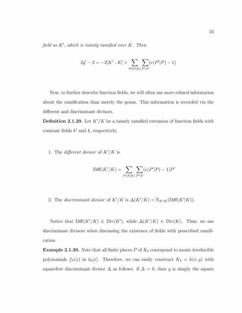
Definition 2.1.29. Let K ′/K be a tamely ramified extension of function fields with

constant fields k′ and k, respectively.

1. The different divisor of K ′/K is

Diff(K ′/K) =∑

P∈P(K)

∑P ′|P

(e(P ′|P )− 1)P ′

2. The discriminant divisor of K ′/K is ∆(K ′/K) = NK′|K(Diff(K ′|K)).

Notice that Diff(K ′/K) ∈ Div(K ′), while ∆(K ′/K) ∈ Div(K). Thus, we use

discriminant divisors when discussing the existence of fields with prescribed ramifi-

cation.

Example 2.1.30. Note that all finite places P of K0 correspond to monic irreducible

polynomials fP (x) in k0[x]. Therefore, we can easily construct K2 = k(x, y) with

squarefree discriminant divisor ∆ as follows: if ∆ = 0, then y is simply the square

25

root of a nonsquare in k0. If ∆ 6= 0, then there are two possibilities for K2, either

y2 =∏

P∈Supp ∆P finite

fP (x),

y2 = c∏

P∈Supp ∆P finite

fP (x).

where c is a nonsquare in k. These quadratic function fields are called twists of each

other.

The different and discriminant divisors of towers of extensions are related as fol-

lows.

Proposition 2.1.31. Let K ′′/K ′/K be extensions of function fields. Then

1. Diff(K ′′/K) = ConK′′/K′(Diff(K ′/K)) + Diff(K ′′/K ′).

2. ∆(K ′′/K) = [K ′′ : K ′] ·∆(K ′/K) + NK′/K(∆(K ′′/K ′)).

Notice that a place appears in the support of ∆(K ′/K) (and Diff(K ′/K)) if and

only if it is ramified.

We now have the background to state the general aims of this work; namely to

efficiently construct certain types of function fields with a given discriminant divisor,

and to tabulate all such fields whose discriminant divisor’s degree is below a fixed

bound. Understanding the types of such fields is the first aim of the following section.

26

2.2 Galois Representations and L-functions

In this section we present the basic concepts from Galois theory and representation

theory in order to describe Artin L-functions. A broader treatment of Galois theory

can be found in many texts such as [17]. The representation theory is mainly from

[34] and the introduction to L-functions of function fields primarily from [37] and [41].

Throughout this section, let K ′/K be a finite extension of function fields.

2.2.1 Galois Theory of Function Fields

We begin by recalling some basic facts from Galois theory of finite extensions of fields.

Definition 2.2.1. Consider the automorphism group

Aut(K ′/K) = {γ ∈ Aut(K ′) : γ(α) = α, ∀α ∈ K} .

An extension is called Galois if |Aut(K ′/K)| = [K ′ : K], in which case we write

Gal(K ′/K) = Aut(K ′/K). The Galois closure of K ′ is the smallest K ′′/K ′ such that

K ′′/K is Galois.

Example 2.2.2. All quadratic function fields with char(k) 6= 2 are Galois. Let

K2 = k(x)[y]/〈y2 − h(x)〉 with char(k) 6= 2, then Gal(K2/K(x)) = {id, τ} where

τ(y) = −y 6= y and τ(α) = α, ∀α ∈ K(x). Here τ is called the quadratic involution

of K2/k(x).

When K ′/K is not Galois, we will often make the common abuse of language

referring to the Galois group of K ′/K when in fact we mean the Galois group of its

Galois closure. We now recall the fundamental theorem of Galois theory.

Theorem 2.2.3 ([37] Appendix A.12). Let K ′′/K be Galois. There is a one-to-one

27

Figure 2.1:

K2`

K`

2

K2

`

〈σ〉

K0

2

〈τ〉`

correspondence between the subfields K ′ of K ′′ containing K and the subgroups of

Gal(K ′′/K); namely the subgroup H of Gal(K ′′/K) corresponds to the fixed field of

H, Fix(H) = {α ∈ K ′ : γ(α) = α, ∀γ ∈ H}. Moreover, K ′/K is Galois if and only if

H is normal in Gal(K ′′/K).

Example 2.2.4. Let ` be an odd prime. Consider the diagram of function fields

presented in Figure 2.1. Here, the field K0 is a rational function field with constant

field k0 with characteristic different from 2 and `. The field K2` is the Galois closure

of K` with Galois group D`, the dihedral group with 2` elements. K2 is the fixed field

of the unique index 2 subgroup C` of D` generated by σ. As C` is normal in D`, K2 is

indeed Galois with Gal(K2/K0) generated by τ . K` is the fixed field of an element of

order 2 in D`. We note that there are ` such elements in D` which give ` conjugate

subfields K` of K2`. The field K2 is called the quadratic resolvent field of K`.

The Galois group of an extension K ′/K has a profound effect on the splitting

behavior of the places of K ′.

Theorem 2.2.5 ([37] Thm 3.7.1). Let K ′/K be a Galois extension of function fields.

Let P ′1, P′2 ∈ P(K ′) lie over a place P ∈ P(K). Then there exists an element γ ∈

Gal(K ′/K) such that P ′2 = γ(P ′1). Moreover, vP ′2(α) = vP ′1(γ−1(α)).

28

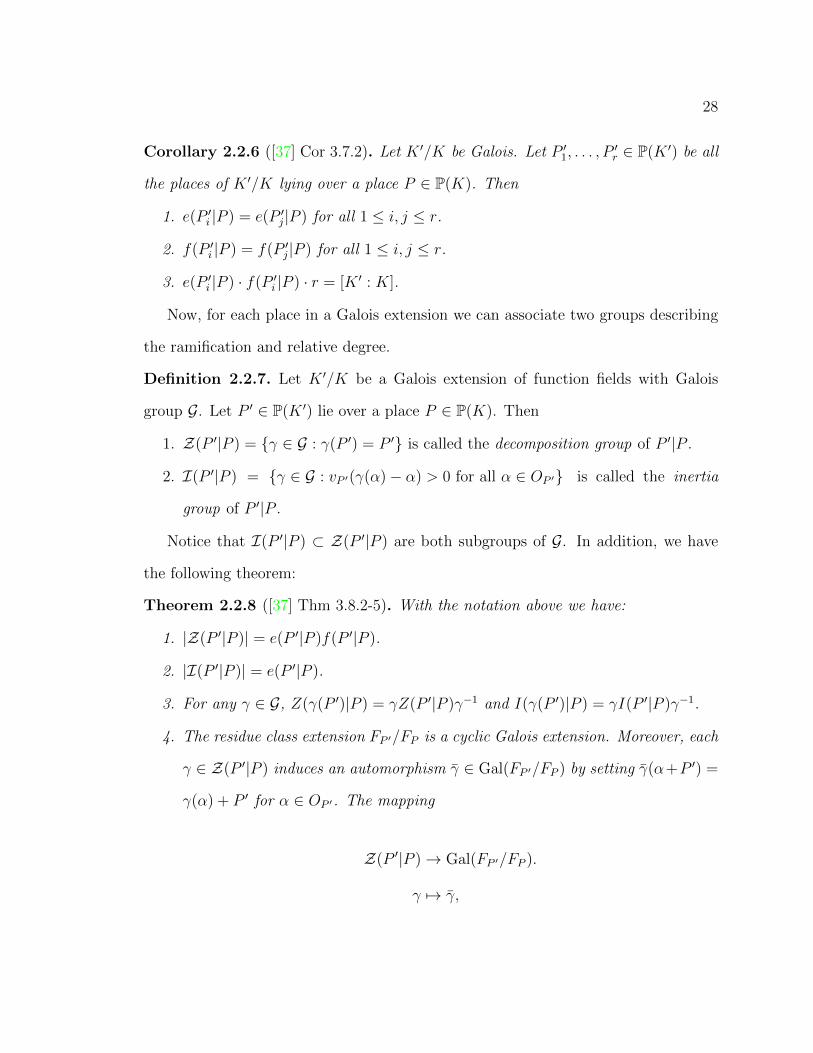
Corollary 2.2.6 ([37] Cor 3.7.2). Let K ′/K be Galois. Let P ′1, . . . , P′r ∈ P(K ′) be all

the places of K ′/K lying over a place P ∈ P(K). Then

1. e(P ′i |P ) = e(P ′j|P ) for all 1 ≤ i, j ≤ r.

2. f(P ′i |P ) = f(P ′j|P ) for all 1 ≤ i, j ≤ r.

3. e(P ′i |P ) · f(P ′i |P ) · r = [K ′ : K].

Now, for each place in a Galois extension we can associate two groups describing

the ramification and relative degree.

Definition 2.2.7. Let K ′/K be a Galois extension of function fields with Galois

group G. Let P ′ ∈ P(K ′) lie over a place P ∈ P(K). Then

1. Z(P ′|P ) = {γ ∈ G : γ(P ′) = P ′} is called the decomposition group of P ′|P .

2. I(P ′|P ) = {γ ∈ G : vP ′(γ(α)− α) > 0 for all α ∈ OP ′} is called the inertia

group of P ′|P .

Notice that I(P ′|P ) ⊂ Z(P ′|P ) are both subgroups of G. In addition, we have

the following theorem:

Theorem 2.2.8 ([37] Thm 3.8.2-5). With the notation above we have:

1. |Z(P ′|P )| = e(P ′|P )f(P ′|P ).

2. |I(P ′|P )| = e(P ′|P ).

3. For any γ ∈ G, Z(γ(P ′)|P ) = γZ(P ′|P )γ−1 and I(γ(P ′)|P ) = γI(P ′|P )γ−1.

4. The residue class extension FP ′/FP is a cyclic Galois extension. Moreover, each

γ ∈ Z(P ′|P ) induces an automorphism γ ∈ Gal(FP ′/FP ) by setting γ(α+P ′) =

γ(α) + P ′ for α ∈ OP ′. The mapping

Z(P ′|P )→ Gal(FP ′/FP ).

γ 7→ γ,

29

is a surjective homomorphism with kernel I(P ′|P ).

5. If |G| is relatively prime to char(K) > 0, then I(P ′|P ) is a cyclic group.

2.2.2 Representation Theory

The Galois group also plays a crucial role in determining the ramification of all the

intermediate fields of K ′/K. To make this apparent we use the theory of L-functions

together with information gained by examining the representations of the Galois

group. Throughout this section, let G denote a finite group and V a finite-dimensional

complex vector space.

Definition 2.2.9. A representation of G is a homomorphism ρ : G → Aut(V ). When

ρ is given, V is called a representation space of G. The dimension of V is called the

degree of the representation ρ. Two representations ρ, ρ′ are isomorphic if there exists

a linear isomorphism A : V → V ′ such that

Aρ(γ) = ρ′(γ)A ∀γ ∈ G.

The following are examples of representations for an arbitrary group G that will

be particularly useful.

Example 2.2.10. Consider the representation ρ0 : G → C given by ρ(γ) = 1 for all

γ ∈ G. This representation ρ is called the trivial representation. Now, consider that

exists an embedding G → Sn of G into the symmetric group on n elements. Consider

30

the representation ρ± : G → C given by

ρ±(σ) =

1 σ has even parity in Sn,

−1 σ has odd parity in Sn,

This is called a parity representation of G. These are two (typically) nonisomorphic

1-dimensional representations of G.

Example 2.2.11. Consider the |G|-dimensional complex vector space V spanned by

a set of vectors B = {eδ : δ ∈ G}, a basis indexed by the elements of G. Define the

(left) regular representation ρ1 as the homomorphism that linearly extends the action

of G on the basis B given by ρ1(γ)(eδ) = eγδ for all γ ∈ G and eδ ∈ B.

Example 2.2.12. Let H be a subgroup of G. Consider the |G/H|-dimensional com-

plex vector space V spanned by a set of vectors B = {eδH : δH ∈ G/H}, a basis

indexed by the (left) cosets of G/H. Define the (left) induced representation (of the

trivial representation on H) ρH as the homomorphism that linearly extends the action

of G on the basis B given by ρH(γ)(eδH) = e(γδ)H for γ ∈ G, eδH ∈ B. Notice that

when H is 〈1〉, the induced representation is isomorphic to the regular representation

and hence the notation is consistent. Also notice that ρG is the trivial representation.

Definition 2.2.13. Let ρ be a representation of G with representation space V . Let

W be a subspace of V . A subspace W of V is said to be G-stable if for all w ∈ W ,

ρ(γ)(w) = w for all γ ∈ G. Then the restriction of ρ to W is a representation called

a subrepresentation of V . A representation is called irreducible if it has no G-stable

subrepresentations.

Theorem 2.2.14 ([34] Ch 1 Thms 1,2). Let ρ : G → Aut(V ) be a representation

31

and let W be a G-stable subspace of V . Then there exists a complement W o of W

in V that is stable under G. Consequently, every representation is a direct sum of

irreducible representations.

We will write ρ1 ⊕ ρ2 for the direct sum of two representations ρ1 : G → V1 and

ρ2 : G → V1, which acts on the space V1 ⊕ V2 component-wise.

The following example demonstrates a decomposition of a representation.

Example 2.2.15. Let D` be the dihedral group of 2` elements for an odd prime `.

Consider the natural embedding of D` into S`. Let V be a complex `-dimensional

vector space with basis {ei}. Then, D` naturally acts on V by permutation on the

basis vectors. Call this representation ρ. Now, ρ has D`-stable subspaces

W = {c0e1 + c0e2 + · · ·+ c0e` : c0 ∈ C} ,

WO ={c1e1 + c2e2 + · · ·+ c`e` :

∑`i=1 ci = 0, ci ∈ C

}.

In fact, V = W ⊕ WO, and thus ρ = ρ|W ⊕ ρ|WO . Notice that ρ|W is the trivial

representation and hence irreducible. However, it can be shown that ρ|WO is reducible

when ` > 3 as there are no irreducible representations of D` of degree greater than 2,

so this is not the full decomposition of ρ into irreducible representations.

To each representation we associate a function to characterize that representation.

Definition 2.2.16. Let ρ : G → Aut(V ) be a representation. The character χρ of ρ

is defined to be

χρ(γ) = Tr(ρ(γ)) for all γ ∈ G,

where Tr denotes the trace of ρ(γ) (the sum of the eigenvalues of ρ(γ), or equivalently,

the sum of the diagonal entries).

32

Throughout, we will let χH denote the character of the induced representation ρH

corresponding to a subgroup H of a group G.

Proposition 2.2.17 ([34] Ch 2). If χ is the character of a representation ρ of degree

n, then

1. χ(1) = n.

2. χ(γ−1) = χ(γ), the complex conjugate of χ(γ), for all γ ∈ G.

3. χ(γδγ−1) = χ(δ) for all γ, δ ∈ G.

Moreover, if ρ1, ρ2 are representations with respective characters χ1 and χ2, then the

character of ρ1 ⊕ ρ2 is χρ1 + χρ2. Lastly, ρ1 and ρ2 are isomorphic if and only if

χ1 = χ2.

Through the above proposition, we can see that characters play an important role

in classifying representations. In particular, we can use characters to find relationships

between induced representations.

Example 2.2.18. Consider the characters of the induced representations of the var-

ious subgroups of D`. Write

D` =⟨σ, τ : σ` = 1, τ 2 = 1, τστ = σ−1

⟩.

By Proposition 2.2.17 we need only consider the values of these characters on conju-

gacy classes of elements, i.e. on the set

C = {[1], [τ ]} ∪{

[σi] = [σ−i] : 1 ≤ i ≤ (`− 1)/2}

where [γ] denotes the conjugacy class of γ ∈ D`.

1. The trivial representation ρD`(inducing the entire group) is a 1-dimensional

33

Table 2.1: Induced Character Table of the Dihedral Group D`χD`

χ1 χC` χC2[1] 1 2` 2 `[τ ] 1 0 0 1{[σi]} 1 0 2 0

representation where χD`(γ) = 1 for all γ ∈ D`.

2. The regular representation ρ1 (inducing the trivial subgroup) is a 2`-dimensional

representation; thus, χ1(1) = 2`. As left multiplication by a nontrivial element

in a group has no fixed points, χ1(γ) = 0 for all 1 6= γ ∈ D`.

3. The representation ρC` (inducing the order ` cyclic subgroup generated by σ)

is a 2-dimensional representation; thus, χC`(1) = 2. As τ 6∈ C`, τ permutes the

cosets C`, τC`, and thus χC`(τ) = 0. Lastly, all other classes of elements in D`

are in C`, and thus act trivially. Hence, χ([σi]) = 2 for all conjugacy classes

[σi] ∈ C.

4. The representation ρC2 (inducing the order 2 cyclic subgroup generated by τ)

is an `-dimensional representation; thus, χC2(1) = `. As τ ∈ C2, τ fixes the

coset C2. Moreover, τσiC2 = σ−iτC2 = σ−iC2, and so τ fixes no other cosets of

D`/C2. Hence χC2(τ) = 1. Lastly, the other classes [σi] act on D`/C2 like cyclic

permutations and thus fix no cosets. Hence, χ([σi]) = 0 for all conjugacy classes

[σi] ∈ C2.

We summarize the above information in Table 2.1.

From Table 2.1 we can see that we have the following relationship between these

induced representations:

2χD`+ χ1 = χC` + 2χC2 . (2.1)

34

2.2.3 L-functions

L-functions provide a means for converting information about Galois groups and their

representations into information about the underlying function fields. In particular,

we will see how to use (2.1) to further understand the ramification of dihedral ex-

tensions. We begin by recalling the zeta functions of function fields. These functions

have a rich and extensive theory. Only the few results required for the purpose of

relating subfields of Galois extensions are presented (for more information, see [37],

Chapter 5). Throughout this section, K will be a function field whose field of con-

stants is k = Fq, and F [[t]] will denote the ring of formal power series in t over a

field F .

Definition 2.2.19. Define N(D) = qdeg(D) as the absolute norm of a divisor D. Then

the power series

ζK(s) =∑

D∈Div(K)D≥0

N(D)−s ∈ Z[[q−s]]

is called the zeta function of K. For simplicity, we make the change of variable t = q−s

and define ZK(t) = ζK(s), and also call this the zeta function of K.

Zeta functions have the following remarkable properties:

Proposition 2.2.20 ([37], Sect 5.1). Let Z(t) denote the zeta function of K. Then

1. Z(t) is absolutely convergent for |t| < q−1.

2. For |t| < q−1, Z(t) has a convergent Euler product:

Z(t) =∏

P∈P(K)

(1− tdeg(P ))−1.

35

3. Z(t) satisfies a functional equation:

Z(t) = (√qt)2g−2Z

(1

qt

).

where g is the genus of K.

Example 2.2.21. Let K be a function field of genus 0, i.e K = Fq(x). Then

ZK(t) =1

(1− t)(1− qt).

Now, to define a zeta function associated to a Galois representation, we present a

Corollary of Theorem 2.2.8 describing the action of Frobenius on a vector space.

Corollary 2.2.22. Let ρ be a representation of Gal(K ′/K) on a complex vector space

V . Let P ′ ∈ P(K ′) be a place lying over P ∈ P(K). Let W denote the subspace of V

fixed by I(P ′|P ). As F ′P/FP∼= Fqf(P ′|P ), let frP ′ denote the generator of Gal(F ′P/FP )

that corresponds to the q-power Frobenius automorphism of Fqf(P ′|P ). Furthermore,

let FrP ′ denote a pre-image of frP ′ under the map of Theorem 2.2.8, part 3. Then

ρ|W (FrP ′) ∈ Aut(W ) is well defined up to conjugacy; i.e. its characteristic polynomial

is independent of the choice of pre-image FrP ′.

From the corollary above, to each place P ′ of a function field we can now associate

a particular linear transformation ρ|W (FrP ′). Each of these transformations will give

rise to a factor in an Euler product, the combination of which will form an L-function.

Definition 2.2.23. With the notation of Corollary 2.2.22, let 1W denote the identity

automorphism of W . Define the Euler factor of P ′ as

LP ′(ρ, t) = det(

1W − ρ|W (FrP ′)tdeg(P ′)

)−1

,

36

i.e. the inverse of the characteristic polynomial of ρ(FrP ′)|W evaluated at tdeg(P ′).

Moreover, define the L-function of ρ to be

L(ρ, t) =∏

P ′∈P(K′)

LP ′(ρ, t).

Notice that this is indeed a generalization of Z(t) in the sense that if ρ0 is the trivial

representation, then ZK′(t) = L(ρ0, t). In fact, L(ρ, t) has some similar properties to

Z(t).

Proposition 2.2.24 ([30] Thm 9.25). Let L(ρ, t) denote the L-function of K associ-

ated to the representation ρ. Then

1. L(ρ, t) is absolutely convergent for |t| < q−1.

2. L(ρ, t) can be extended to a meromorphic function on C.

Furthermore, L-functions can be decomposed with respect to the decomposition

of their representation. In particular, we have the following proposition which will be

utilized in the next section.

Proposition 2.2.25 ([2]). Let K ′/K be a Galois extension with Galois group G, and

let H be a subgroup of G. Let ρ, ρ′ be representations of G. Then

1. L(ρ⊕ ρ′, t) = L(ρ, t)L(ρ′, t).

2. L(ρH, t) = ZFix(H)(t).

2.3 Dihedral Function Fields

The main goal of this section is to compute the discriminant divisor of a degree `

dihedral function field. The results of this section are my own work and first appeared

in [42].

37

We begin by recalling the situation in Example 2.2.4. From here on we fix all the

following notation. Let ` be an odd prime. Recall, the diagram of subfields given in

Figure 2.1:

K2`

K`

2

K2

`

〈σ〉

K0

2

〈τ〉`

Recall that K0 is a rational function field, and the field K2` is the Galois closure

of K` with Galois group D`, the dihedral group with 2` elements. Recall further that

K2 is the quadratic resolvent, i.e the fixed field of the unique index 2 subgroup C` of

D` generated by σ. K` is the fixed field of τ , the generator of C2 in D`.

To prove the main theorem, we will use the following supporting lemma:

Lemma 2.3.1. The discriminant divisor ∆(K`/K0) satisfies

deg(∆(K`/K0)) =`− 1

2(deg(∆(K2/K0)) + deg(M)) ,

where M ∈ Div(K) is defined via (`− 1)M = NK2/K0(∆(K2`/K2)).

Proof. By (2.1), the induced characters χ1, χD`, χC2 , χC` are linearly dependent, and

thus by Proposition 2.2.17, the representations ρ1, ρD`, ρC2 , ρC` satisfy

ρ1 ⊕ 2ρD`∼= 2ρC2 ⊕ ρC` .

38

By parts 1 and 2 of Proposition 2.2.25, we have

ZK2`(t)ZK0(t)

2 = ZK`(t)2ZK2(t).

From the functional equation of the zeta function (part 4, Proposition 2.2.20) we

obtain

(2gK2`− 2) + 2(2gK0 − 2) = 2(2gK`

− 2) + (2gK2 − 2).

Applying Theorem 2.1.26, we have

deg(∆(K2`/K0)) + 2 deg(∆(K0/K0)) = 2 deg(∆(K`/K0)) + deg(∆(K2/K0)),

deg(∆(K2`/K0)) = 2 deg(∆(K`/K0)) + deg(∆(K2/K0)). (2.2)

By Proposition 2.1.31,

∆(K2`/K0) = [K2` : K2]∆(K2/K0) + NK2/K0(∆(K2`/K2)).

As K2`/K2 is a cyclic Galois extension, by Theorem 2.1.18, for all places P ′′ ∈

Supp(∆(K2`/K2)) lying over a place P ′ ∈ P(K2), e(P ′′|P ′) divides [K2` : K2] = `

and hence e(P ′′|P ′) = `. Consequently,

∆(K2`/K2) = (`− 1)M ′,

where M ′ ∈ Div(K2) is the sum of the ramified places of K2`/K2. Therefore,

NK2/K0(∆K2`/K2) = (` − 1)M where M = NK2/K0(M′). Now, (2.2) can be rewrit-

39

ten as

` deg(∆(K2/K0)) + (`− 1) deg(M) = 2 deg(∆(K`/K0)) + deg(∆(K2/K0)).

Thus,

deg(∆(K`/K0)) =`− 1

2(deg(∆(K2/K0)) + deg(M)).

Theorem 2.3.2. The discriminant divisor ∆(K`/K0) satisfies

∆(K`/K0) =`− 1

2(∆(K2/K0) +M) ,

where (`− 1)M = NK2/K(∆(K2`/K2)), and M and ∆(K2/K0) are coprime.

Proof. Let E = `−12

(∆(K2/K0) + (` − 1)M). First note that the only places of

K0 ramified in K` are those lying over places in the support of M and ∆K2 , as

K2`/K2/K0 is only ramified at these places. As D` is not cyclic, by Theorem 2.2.8,

there are no places P ′′ ∈ P(K2`) such that e(P ′′|P ) = 2`, and hence Supp(M) and

Supp(∆(K2/K0)) are disjoint. Thus, for all places P ∈ Supp(M) and all P ′′ ∈ P(K2`)

lying over P , e(P ′′|P ) = `. Similarly, for all places P ∈ Supp(∆(K2/K0)) and all

P ′′ ∈ P(K2`) lying over P , e(P ′′|P ) = 2. As [K2` : K`] = 2 - `, all places P ′ ∈ P(K`)

lying over M must have e(P ′|P ) = `. Also, for all P ′ ∈ P(K`) lying over ∆K2 ,

e(P ′|P ) ≤ 2. Applying the identity

∑P ′|P

e(P ′|P )f(P ′|P ) = `

40

to any place P ∈ Supp(∆(K2/K0)) allows at most (`− 1)/2 places P ′|P of K` to be

ramified. Thus, ∆(K`/K0) divides E. Since both divisors have the same degree, they

must be equal.

Remark 2.3.3. While we only presented a proof of Theorem 2.3.2 for the case when

the coefficient field k0 of K0 is a finite field, Theorem 2.3.2 in fact holds when k0 is

an arbitrary perfect field with characteristic not dividing 2`. For brevity we omit the

details, but one could prove this by careful examination of the higher ramification

groups of K2`/K0. When char(k0) - 2`, the inertia groups are cyclic and all higher

ramification groups are trivial. Moreover, the only nontrivial cyclic subgroups of D`

are C` and C2. As K`/K0, is the fixed field of τ , K2`/K` is ramified at the places where

τ fixes their interia groups, i.e. those places whose interia group is C2. Proposition

2.1.17 then completes the proof of Theorem 2.3.2. Again, to avoid expounding further

upon these topics, we leave the details of this proof to the reader.

In this chapter we defined the fundamental theory required to prove the results of

this last section. Having touched upon the theory of function fields, representation

theory, Galois theory, and the theory of L-functions, we were able to show the precise

relationship between the ramification of a degree ` dihedral function field and that of

its quadratic resolvent and Galois closure. Using this information, the remaining goal

of this thesis is to construct and tabulate all dihedral function fields with prescribed

ramification.

The aim of the next three chapters describe different methods for constructing

all dihedral extensions of odd prime degree. As we saw in Example 2.2.4, dihedral

function fields are uniquely determined (up to Galois conjugacy) by their Galois

closures. Thus, our general approach for constructing dihedral function fields will

41

be to first construct their Galois closures, then compute the degree ` subfield by

computing the fixed field of an automorphism of order 2. We also saw in Example

2.2.4 that degree 2` dihedral function fields are degree ` cyclic extensions of quadratic

fields (the quadratic resolvent). From Theorem 2.3.2, the discriminant divisor of a

degree ` dihedral function field can be computed in terms of the discriminant divisor

of its quadratic resolvent and the discriminant divisor of the degree ` cyclic extension

thereof. Moreover, quadratic function fields are uniquely determined (up to twist) by

their discriminant divisors. Hence, to construct degree ` dihedral function fields of

a given discriminant divisor, we have reduced the problem to constructing all cyclic

degree ` extensions of a given quadratic function field, with prescribed ramification.

42

Chapter 3

Construction of Dihedral Function

Fields via Class Field Theory

Having introduced the foundations of dihedral function fields, we now proceed by

describing our first method for constructing all dihedral extensions of odd prime

degree and given ramification; namely via class field theory. In this chapter we

will present two algorithms. The first algorithm will construct all degree ` dihedral

function fields with a given discriminant divisor and fixed quadratic resolvent. Using

the first algorithms, we produce another method for constructing all degree ` dihedral

function fields with a given discriminant divisor (with any possible the quadratic

resolvent).

The results of this chapter are similar to those found in [8] (which is based on

[19]) for the number field setting; they are however my own work and not mentioned

in [42]. We also note that recently (after I had developed this work) this method was

presented in [28] for the case ` = 3. To the best of my knowledge, the remaining

cases are not covered elsewhere in the literature, though it would not be surprising if

others were aware of this technique for other values of `.

Recall that we have reduced the problem of constructing degree ` dihedral function

fields of a given discriminant divisor to that of constructing all cyclic Galois degree

43

` extensions of a given quadratic function field with prescribed ramification. Class

field theory is the study of abelian extensions, and as such, it is the natural place to

begin.

Throughout this chapter, K will be a function field with finite constant field k.

3.1 Class Fields of Function Fields

We begin our introduction to class field theory by returning again to Galois theory.

Definition 3.1.1. Let K ′/K be a Galois extension of function fields with Galois

group G. Let P ′1 and P ′2 be two unramified places of K ′ lying over a place P ∈ P(K).

Define the Artin conjugacy class (P,K ′/K) ⊂ G to be the set of FrP ′ ∈ G for all

P ′|P .

Since the above places are assumed to be unramified, their Frobenius elements

FrP ′ are well defined in G. By Theorem 2.2.8, the two decomposition groups Z(P ′1|P )

and Z(P ′2|P ) are conjugate subgroups of G. Hence (P,K ′/K) is well defined and

indeed a conjugacy class of G.

Now, and for the remainder of this section, assume that K ′/K is a finite abelian

Galois extension of function fields. Then (P,K ′/K) is in fact a single automorphism.

Hence we can define a map from the unramifield places of K ′/K to G.

Definition 3.1.2. Let S = S(K ′/K) ⊂ P(K) denote the set of places of K ramified

in K ′. Let DivS(K) be the subgroup of Div(K) consisting of the divisors whose

support is disjoint from S. The Artin map (∗, K ′/K) : DivS(K)→ Gal(K ′/K) is the

homomorphism extending the map defined by P 7→ (P,K ′/K) to DivS(K), where

P ∈ P(K).

The Artin map relates Galois groups to divisor groups in a precise way. This

44

relationship is made more explicit by the following proposition:

Proposition 3.1.3 ([30] Prop 9.18). Let S ′ = S ′(K ′/K) denote the set of P ′|P where

P ∈ S(K ′/K) and let DivS′(K′) be the subgroup of Div(K ′) consisting of the divisors

whose support is disjoint from S ′. Then the Artin map is onto and its kernel contains

the group NK′/K(DivS′(K′)).

To understand the kernel of the Artin map, we present ray class groups.

Definition 3.1.4. Let M =∑nPP be a divisor of K. The ray modulo M is the

subgroup of Prin(K) given by

RM(K) = {(α) ∈ Prin(K) : vP (α− 1) ≥ nP , ∀P ∈ Supp(M)}.

Let PrinM(K) denote the principal divisors of K supported away from M . Then

RM(K) is a subgroup of PrinM(K), and thus a subgroup of DivS(K). The ray class

group modulo M is the quotient group ClM(K) = DivS(K)/RM(K).

We note that every ray class group ClM(K) is infinite. There is a natural degree

map on ClM(K) that induces the following exact sequence:

1→ Cl0M(K)→ ClM(K)→ Z→ 1,

where Cl0M(K) denotes the ray classes of degree 0. We remark that Cl0M(K) is finite

and thus sometimes called the ray class group in the literature to align with the

number field situation in that regard. We will refer to Cl0M(K) as the degree zero ray

class group modulo M .

We can now describe the kernel of the Artin map.

Theorem 3.1.5 ([7] Ch 7, Sect 5, Thm 5.1). Let K ′/K, S = S(K ′/K), and S ′ =

45

S ′(K ′/K) as above. Then the following hold:

1. Artin Reciprocity Theorem: The Artin map is onto and there exists an ef-

fective divisor M supported on S such that the kernel of the Artin map is

PrinM(K) NK′/K(DivS′(K′)). Consequently, the Artin Map induces an isomor-

phism

ClM(K)/〈[NK′/K(DivS′(K′))]〉 ∼= Gal(K ′/K).

where 〈[NK′/K(DivS′(K′))]〉 denotes the subgroup of ClM(K) generated by the

classes of the elements in NK′/K(DivS′(K′)).

2. Takagi Existence Theorem: For each subgroup H of finite index in ClM(K) there

exists a unique abelian extension K ′/K such that 〈[NK′/K(DivS′(K′))]〉 = H.

Remark 3.1.6. Considering Theorem 3.1.5, we can see that every abelian extension

of a function field can be understood via its ray class groups and, more generally,

via class field theory. This pursuit is well beyond the scope of this thesis (see [41]

and [7] for more details); however, we require further results from class field theory

to construct all dihedral function fields of a given discriminant divisor. While we

have presented the required background to state these results, the material required

to understand their proofs, including that of Theorem 3.1.5, is not covered in this

thesis. These results are very deep; their proofs rely on local class field theory, infinite

Galois theory, and the theory of Drinfeld modules, to name a few ingredients.

By Theorem 3.1.5, and the universal property of inverse limits, there exists a

unique (within a fixed algebraic closure) infinite Galois extension KM with the prop-

erty that Gal(KM/K) = ClM(K). The function field KM is called the ray class field

modulo M . Notice that Theorem 3.1.5 says that every abelian extension of K is a

subfield of a ray class field of K.

46

Notice too that the Artin Reciprocity Theorem only claims the existence of an

effective divisor M . There are in fact many possible divisors M for which the Artin

Reciprocity Theorem holds. In particular, if M1 < M2 (with “<” as in Definition

2.1.22), then ClM1(K) ⊂ ClM2(K). However, there is a unique minimal choice of

M under this ordering called the conductor of K ′/K. The conductor of a subgroup

H ⊂ RM is defined to be the conductor of the field corresponding to H in part 2 of

Theorem 3.1.5. Putting this together, we see that every field of conductor M is a

subfield of the ray class field modulo M , and the ray class field modulo M contains

all abelian extensions with conductor less than or equal to M .

From Theorem 3.1.5 we also see that the conductor of K ′/K is related to the

discriminant divisor of K ′/K, as both are supported at the ramified places. We make

this relationship explicit for the particular extensions of interest to this thesis with

the following proposition:

Proposition 3.1.7 ([41] Thm 12.6.39). Let ` be a prime. Let K ′/K be a degree `

tamely ramified cyclic Galois extension of function fields. Let M ∈ Div(K) be the

sum of the places of K ramified in K ′. Then the conductor of K ′/K is M , and

∆(K ′/K) = (`− 1)M .

3.2 Class Field Theoretic Construction Algorithms

In this section we present an algorithm for constructing all degree ` dihedral function

fields with a given discriminant divisor. As explained before, we do so by constructing

cyclic extensions of their quadratic resolvents.

Let K0/k0 be a rational function field of characteristic different from 2 and `, with

finite constant field k0. We will use the notation of Example 2.2.4, namely that ` is

47

an odd prime, that K0 is a rational function field, and that the field K2` is the Galois

closure of K` with Galois group D`. Recall further that K2 is the quadratic resolvent

of K`, i.e. the fixed field of the unique index 2 subgroup C` of D` generated by σ. K`

is the fixed field of τ , the generator of C2 in D`. Also recall from Theorem 2.3.2 that

∆(K`/K0) =`− 1

2(∆(K2/K0) +M) ,

where (` − 1)M = NK2/K((` − 1)M ′), with M ′ defined by (` − 1)M ′ = ∆(K2`/K2).

By Proposition 3.1.7, M ′ is the conductor of K2`/K2.

We saw in the previous section that every abelian extension of a function field

is a subfield of a ray class field. Moreover, for the case of tamely ramified cyclic

extensions of prime degree, we saw in Proposition 3.1.7 that the discriminant divisor

of that extension is determined by its conductor. Consequently, we have a method to

compute all degree ` dihedral function fields of a given discriminant divisor and fixed

quadratic resolvent; namely by computing all degree ` subfields of the appropriate ray

class field. Thus, Theorem 3.1.5 and Proposition 3.1.7 lead directly to Algorithm 3.1.

This algorithm cannot actually be implemented in Magma as written. While

Magma can compute the Galois group of a function field, it does not return the

actual Galois automorphisms (the group is returned abstractly). Thus, we cannot

compute the fixed field of an element of order 2 in Gal(K2`/K0) in this manner. One

could potentially compute a lift of τ to K2` and use Magma’s fixed field methods.

Using such a lift, we will compute the defining equation for K` directly from a defining

equation of K2`/K2 via the following proposition:

Proposition 3.2.1. With the notation above, let f(Y ) be a defining polynomial of

48

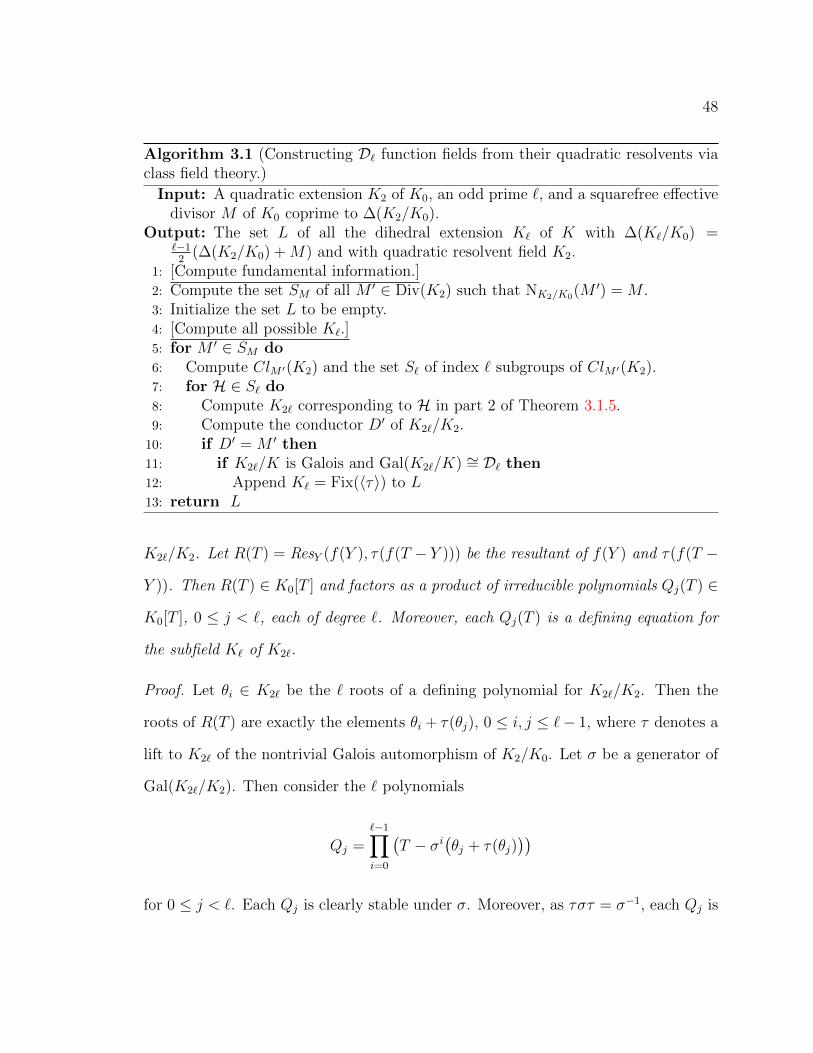
Algorithm 3.1 (Constructing D` function fields from their quadratic resolvents viaclass field theory.)

Input: A quadratic extension K2 of K0, an odd prime `, and a squarefree effectivedivisor M of K0 coprime to ∆(K2/K0).

Output: The set L of all the dihedral extension K` of K with ∆(K`/K0) =`−1

2(∆(K2/K0) +M) and with quadratic resolvent field K2.

1: [Compute fundamental information.]2: Compute the set SM of all M ′ ∈ Div(K2) such that NK2/K0(M

′) = M .3: Initialize the set L to be empty.4: [Compute all possible K`.]5: for M ′ ∈ SM do6: Compute ClM ′(K2) and the set S` of index ` subgroups of ClM ′(K2).7: for H ∈ S` do8: Compute K2` corresponding to H in part 2 of Theorem 3.1.5.9: Compute the conductor D′ of K2`/K2.10: if D′ = M ′ then11: if K2`/K is Galois and Gal(K2`/K) ∼= D` then12: Append K` = Fix(〈τ〉) to L13: return L

K2`/K2. Let R(T ) = ResY (f(Y ), τ(f(T − Y ))) be the resultant of f(Y ) and τ(f(T −

Y )). Then R(T ) ∈ K0[T ] and factors as a product of irreducible polynomials Qj(T ) ∈

K0[T ], 0 ≤ j < `, each of degree `. Moreover, each Qj(T ) is a defining equation for

the subfield K` of K2`.

Proof. Let θi ∈ K2` be the ` roots of a defining polynomial for K2`/K2. Then the

roots of R(T ) are exactly the elements θi + τ(θj), 0 ≤ i, j ≤ `− 1, where τ denotes a

lift to K2` of the nontrivial Galois automorphism of K2/K0. Let σ be a generator of

Gal(K2`/K2). Then consider the ` polynomials

Qj =`−1∏i=0

(T − σi

(θj + τ(θj)

))for 0 ≤ j < `. Each Qj is clearly stable under σ. Moreover, as τστ = σ−1, each Qj is

49

stable under τ as well. Consequently Qj ∈ K0[T ] and hence so is R(x).

We claim that Qj is the minimal polynomial of θj + τ(θj) which is an element of

some index 2 subfield of K2(θ). As θj + τ(θj) is invariant under τ , it lies in its fixed

field. However, as it is not invariant under σ, it does not lie in K0. Thus, as ` is

prime, θj+τ(θj) ∈ K` for some K2(θ)/K`/K0 with [K2(θ) : K`] = 2. Hence, θj+τ(θj)

has a degree ` monic irreducible minimal polynomial mj ∈ K0[T ]. As θj + τ(θj) is a

root of Qj, mj divides Qj. However, Qj is also a monic polynomial of degree `, and

therefore mj = Qj.

Now, all the index two subfields of K2` are Galois conjugate and hence can be

defined by the same minimal polynomial. So there are ` possible choices of irreducible

factors of R(T ), not necessarily distinct, each one a defining polynomial for the degree

` subfield of K2` (up to Galois conjugation).

We note that each of the statements of Algorithm 3.1 can now be implemented in

Magma almost exactly as written (using Proposition 3.2.1 to compute Fix(τ)).

Example 3.2.2. In this example we perform Algorithm 3.1 for the case ` = 3 and

M = 0. Consider the rational function field K0 = F7(x). Let K2 = F7(x, y) be the

quadratic function field defined by y2 = x(x+ 3)(x+ 1). Then

ClM(K2) ∼= Z/2Z⊕ Z/6Z⊕ Z ∼= 〈[C ′1]〉 ⊕ 〈[C ′2]〉 ⊕ 〈[C ′3]〉,

where

C ′1 = 〈x+ 1, y〉 − 〈x, y〉, C ′2 = 〈x+ 5, y + 3〉 − 〈x, y〉, C ′3 = 〈x, y〉.

50

There are thus 4 index 3 subgroups of ClM(K2):

H1 = 〈[C ′1], 3[C ′2], [C ′3]〉,

H2 = 〈[C ′1], [C ′2], 3[C ′3]〉,

H3 = 〈[C ′1], 3[C ′2], 3[C ′3], [C ′1] + [C ′2]〉,

H4 = 〈[C ′1], 3[C ′2], 3[C ′3], [C ′1] + 2[C ′2]〉.

We compute the fields K6,i/K2 corresponding to Hi under Theorem 3.1.5. Checking

their Galois groups, we find that only K6,1/K0 is dihedral. As the conductor must be

less than or equal to M = 0, we know K6,1/K2 has conductor 0. We then compute

a defining polynomial Y 3 + 4xy + 6x3 ∈ K2[Y ] for K6,1/K2. Now, using Proposition

3.2.1, we compute a defining equation for the field K3/K0 to be T 3 +(x2 +4x)T +5x3,

and find that indeed ∆(K3/K0) = ∆(K2/K0).

Even though Algorithm 3.1 can be implemented in Magma using Proposition 3.2.1,

the generic algorithms available to perform the check if K2` is Galois, and to compute

its Galois group, are very costly. There are however some improvements that can be

made via the following propositions:

Proposition 3.2.3. If K2`/K2 is Galois with conductor M ′, then τ(M ′) = M ′.

Let M = NK2/K0(M′). Then M = 2M0 for some squarefree effective divisor M0 ∈

Div(K0), where ∆(K2/K0) and M0 have disjoint support. Thus M ′ = ConK2/K0(M0).

Proof. If K2`/K2 is Galois with conductor M ′, then a lift of τ fixes K2`, and hence

τ fixes its conductor. Thus, for all P ′ in P(K2), we have P ′ ∈ Supp(M ′) if and

only if τ(P ′) in Supp(M ′). By Theorem 2.3.2, M and ∆(K2/K0) are disjoint; in

particular, no place in Supp(M) ramifies in K2. It follows that M ′ is of the form

51

M ′ = D′ + E ′ where D′ is the sum of both places P ′ of K2 lying above each place

P in Supp(M) that split in K2, and E ′ is the sum of the places P ′ of K2 lying

above the places P ∈ Supp(M) that are inert in K2. Hence, M = 2M0 where

M0 = NK2/K0(D′ + E ′). It is now easy to see that M0 is effective, squarefree, has

support disjoint from ∆(K2/K0), and M ′ = ConK2/K0(M′).

We can now improve Algorithm 3.1 by changing the input to a squarefree effective

divisor M0 instead of a divisor M . Then by the above proposition we need only con-

sider one possibility for M ′ in step 5, thereby effectively removing the loop. Moreover,

we have the following corollary:

Corollary 3.2.4. There are no dihedral function fields K`/K0 with deg(∆(K`/K0)) <

2(`− 1) when k0 is a finite field.

Proof. SupposeK` is aD` extension ofK0 with Galois closureK2` and quadratic resol-

vent K2. Theorem 2.3.2 and Proposition 3.2.3 give ∆(K`/K0) = `−12

∆(K2/K0)+(`−

1)M0. Quadratic extensions have discriminants of even degree and so deg(∆(K`/K0))

is divisible by ` − 1. Therefore, it suffices to rule out the three possibilities when

∆(K2/K0)/2 + deg(M0) ≤ 1.

1. deg(∆(K2/K0) = deg(M0) = 0: In this case, K`/K would be a constant field

extension, and would not have Galois group D`.

2. deg(∆(K2/K0)) = 1, deg(M0) = 0: In this case K2 would have genus 0 and

K2`/K2 would be unramified and hence a constant field extension. So, as K` is

the fixed field of τ , K`/K0 would also be a constant field extension, and hence

K2`/K0 would not be dihedral.

3. deg(∆(K2/K0)) = 0, deg(M0) = 1: In this case, K2/K0 is a constant field ex-

52

tension and M0 is a single place of degree 1; since every place in M0 must split in

K2 or of degree 2. Now, since the places of K0 that split in a quadratic constant

field extension are the places of even degree, we again have a contradiction.

We now show how to verify if K2`/K0 is dihedral.

Proposition 3.2.5. Let M0 be a squarefree effective divisor of K0 that is coprime to

∆(K2/K0), and let M ′ = ConK2/K0(M0). Let H ⊂ ClM ′(K2) be an index ` subgroup

of ClM ′(K2), and let K2`/K2 be the extension corresponding to H via Theorem 3.1.5.

Then the following hold:

1. K2`/K0 is Galois if and only if τ fixes H.

2. Additionally, K2`/K0 is Galois with Galois group D` if and only if τ does not

fix any generator of ClM ′(K2)/H.

Proof. First we show that the ray class field KM ′ is Galois over K0. Clearly, KM ′/K0

is separable and algebraic, thus it remains to show KM ′/K0 is normal. Let Ksep0 be

a fixed separable closure of K0 containing KM ′ . Let ω be an element of order 2 in

Gal(Ksep0 /K0), so that ω is a lift of τ . As KM ′/K2 is Galois and thus normal, KM ′/K0

is normal if and only if ω(KM ′) = KM ′ ([17] p. 631).

First, as KM ′/K2 is abelian, so too is ω(KM ′)/K2. By part 3 of Theorem 2.2.8,

ω(KM ′)/K2 is ramified only at ω(M ′). However, ω(M ′) = τ(M ′) = M ′ by Proposition

3.2.3. Now, as KM ′ is the maximal abelian extension of K2 ramified at M ′, we have

ω(KM ′) ⊂ KM ′ , and hence they are equal. Therefore, KM ′/K0 is normal and thus

Galois.

As K2/K0 is Galois, by Theorem 2.2.3, we see that Gal(KM ′/K2) is a normal

53

subgroup of Gal(KM ′/K0) and thus the following sequence is exact and splits canon-

ically:

1 −→ Gal(KM ′/K2) −→ Gal(KM ′/K0) −→ Gal(K2/K0) −→ 1.

Thus, Gal(KM ′/K0) is isomorphic to Gal(KM ′/K2)o〈τ〉, where τ acts on Gal(KM ′/K2)

by conjugation . Thus, by Theorem 2.2.3, K2`/K0 is Galois if and only if Gal(K2`/K2)o

〈τ〉 is a normal subgroup of Gal(KM ′/K2) o 〈τ〉.

Investigating the action of τ on Gal(KM ′/K2) more explicitly via part 3 of Theo-

rem 2.2.8, we see that the Artin map has the property that

(τ(P ′), KM ′/K2) = (ω(P ′), KM ′/K2) = ω(P ′, KM ′/K2)ω.

for all unramified places P ′ ∈ P(K2). Now, by Theorem 3.1.5, Gal(K2`/K2) ∼=

ClM ′(K2)/H via the Artin map. Therefore K2`/K0 is Galois if and only if Ho 〈τ〉 is

a normal subgroup of ClM ′(K2) o 〈τ〉, where here, via the Artin map, the action of

τ on ClM ′(K2) is the natural action of τ on divisor classes. As ClM ′(K2) is abelian,

Ho 〈τ〉 is a normal subgroup of ClM ′(K2) o 〈τ〉 if and only if τ(H) = H.

Assuming that K2`/K0 is Galois, there are only two possibilities for the group

Gal(K2`/K0); it is either abelian and thus isomorphic to Z/`Z⊕ Z/2Z, or it is non-

abelian, and thus isomorphic to D`. Thus, to prove that the Galois group is D`, we

need only show it is not abelian. If we take [C ′] to be any generator of ClM ′(K2)/H,

then (τ(C ′), K2`/K2) = τ(C ′, K2`/K2)τ , and hence Gal(K2`/K0) is abelian if and

only if the action of τ is trivial, i.e. if and only if τ([C ′]) +H = [C ′] +H.

The above proposition gives a simple criterion to effectively check if K2`/K0 is

Galois and Gal(K2`/K0) ∼= D` in step 11 of Algorithm 3.1. This removes the need

54

to use the slower generic algorithms. Combining this with the previously mentioned

improvement, we present a practical implementation of Algorithm 3.1 in Algorithm

3.2. This was implemented, and the results are discussed further in Chapter 6.

Algorithm 3.2 (Efficiently constructing D` function fields from their quadratic re-solvents via class field theory.)

Input: A quadratic extension K2 of K0, an odd prime `, and an effective squarefreedivisor M0 of K0 coprime to ∆(K2/K0).

Output: The set L of all the dihedral extension K` of K with ∆(K`/K0) =`−1

2∆(K2/K0) + (`− 1)M0 and quadratic resolvent K2.

1: Compute M ′ = ConK2/K0(M0) ∈ Div(K2).2: Initialize the set L to be empty.3: [Compute all possible K`.]4: Compute ClM ′(K2) and the set S` of index ` subgroups of ClM ′(K2).5: for H ∈ S` do6: Compute the conductor D′ of H.7: if D′ = M ′ then8: Compute [DH] +H a generator of ClM ′/H.9: if τ(H) = H and τ([DH]) +H 6= [DH] +H then10: Compute defining equation f(Y ) for K2`/K2 corresponding to H in part 2

of Theorem 3.1.5.11: Compute the resultant R(T ) = ResY (f(Y ), τ(f(T − Y ))12: Factor R(T ) and let Q(T ) be a factor of degree `.13: Append Q(T ) to L2.14: return L

Example 3.2.6. Using the information of Example 3.2.2, we see that [C ′2] +H1 is a

generator of ClM ′(K2)/H1. First we see that τ(C ′1) = C ′1 and τ(C ′3) = C ′3, and hence

55

τ(H1) = H1. We then compute

τ(C ′2) = τ(〈x+ 5, y + 3〉)− τ(〈x, y〉)

= 〈x+ 5, y − 3〉 − 〈x, y〉

= 5C ′2 + 2C ′3

and see that τ([C2]) +H = 2[C ′2] +H. Therefore, K6,1/K0 of Example 3.2.2 is indeed

a dihedral Galois extension by Proposition 3.2.5.

Regardless of any remaining inefficiencies, this approach is broad in its applica-

bility and is practical in many cases. Notice that Algorithm 3.2 does not place severe

restrictions on the underlying constant field, it only requires the constant field to be

finite and of characteristic different from 2 and `. Thus, using Algorithm 3.2, we can

produce a reasonable technique to construct all degree ` dihedral function fields of a

given discriminant divisor. This is presented in Algorithm 3.3.

Algorithm 3.3 takes advantage of the following observation: In order for any de-

gree ` dihedral function fields K` to exist, the discriminant divisor D of its quadratic

resolvent must be effective, squarefree, and of even degree. As we saw in Exam-

ple 2.1.30, if D = 0, then this field is the unique quadratic constant field extension

of K0 which we denote K0. If D is nonzero, then there are exactly two quadratic

function function fields K2 and K2 of discriminant divisor D.

Recall that all finite places P of K0 correspond to monic irreducible polynomials

fP (x) in k0[x]. Therefore, in step 2 of Algorithm 3.3 we can easily construct K2 and

K2 as in Example 2.1.30.

Even with the two improvements resulting from Propositions 3.2.3 and 3.2.5, the

56

Algorithm 3.3 (Constructing D` function fields from their divisors via class fieldtheory.)

Input: An odd prime ` and squarefree effective divisors D and M0 of K0 withdisjoint support.

Output: The set L of all the dihedral extension K` of K0 with ∆(K`/K0) = `−12D+

(`− 1)M0.1: if deg(D) is even then2: Construct a quadratic field K2 with discriminant divisor D.3: else4: return “D is not a quadratic discriminant divisor”.5: [Compute possible K`]6: Initialize the set L to be empty.7: if D = 0 then8: Get L1 from Algorithm 3.2 with input K0, `,M0.9: L← L ∪ L1.10: else11: Construct K2 and K2 of discriminant divisor D.12: Get L1 from Algorithm 3.2 with input K2, `,M0.13: Get L2 from Algorithm 3.2 with input K2, `,M0.14: L← L ∪ L1 ∪ L2.15: return L.

class field theoretic methods of Algorithm 3.2 (and consequently Algorithm 3.3) are

not very efficient. For instance, the built-in function in Magma for computing a

defining equation for K2`/K2 in step 10 of Algorithm 3.2 is quite costly. Indeed,

the method was implemented in Magma by C. Fieker and based upon his number

field algorithm in [19], in which he notes that a “rather surprising bottleneck is the

computation of the minimal polynomials” for cyclic extensions.

Even if some of these built-in functions could be improved upon by specializing

them to computing dihedral extensions, we are still computing more than what is

required. We must compute the conductor of every subgroup produced in step 6 of

Algorithm 3.2; this includes one for every degree ` cyclic field whose conductor divides

57

M ′. While the conductor can be computed group-theoretically without computing

the defining equation of K2`, it still needs to be computed for each subgroup. While

not terribly time consuming, this becomes especially inefficient for inputs M0 with

large support, where many irrelevant subgroups are considered.

Example 3.2.7. Consider the rational function field K0 = F7(x). Let K2 = F7(x, y)

be the quadratic function field defined by y2 = x(x + 3)(x + 1), let M0 = 〈x + 3〉 +

〈x+ 5〉 ∈ Div(K0), and let M ′ = ConK2/K0(M0). Then

ClM ′(K2) ∼= Z/2Z⊕ Z/6Z⊕ Z/6Z⊕ Z/36Z⊕ Z,

and thus ClM ′(K2)/3(ClM ′(K2)) ∼= (Z/3Z)4 . Hence, there are 40 distinct index 3

subgroups of ClM ′(K2), and as we will see in Example 4.2.3, only 3 of these correspond

to dihedral function fields with conductor M ′.

The above example illustrates the inefficiency of Algorithm 3.2 for a conductor M0

of degree only 2. As the degree of M0 grows, so too does the number of extraneous

subgroups of ClM ′(K2) that need to be considered.

The algorithms presented in the next two chapters overcome some of these obsta-

cles. In particular, we will construct all dihedral function fields with the prescribed

discriminant divisors without having to verify any conductors (or discriminant divi-

sors) along the way. Furthermore, in this new method we have an explicit formula

for the defining equation of K`/K0. This avoids the costly computations of finding a

defining equation for K2`/K2 in step 10 of Algorithm 3.2, and factoring (and comput-

ing) a resultant polynomial as in Proposition 3.2.3. A runtime comparison of these

approaches will be provided in Chapter 6.

58

Chapter 4

Kummer Theoretic Approach with

`-th Roots of Unity

In this chapter we will present an algorithm to construct all dihedral function fields

with a given discriminant divisor when the constant field contains the `-th roots of

unity. The construction algorithm is based on the main theorem, which is an exact

count for the number of degree ` function fields with Galois group D` and given

discriminant divisor ∆. Throughout, let ζ` ∈ k0 be a primitive `-th root of unity.

Again for this chapter we will assume that k0 is perfect though not necessarily finite,

with characteristic not dividing 2`. Let k2 denote the constant field of a quadratic

extension K2/k2 of K0/k0. Then k2 is either equal to k0 or is a quadratic extension

thereof. The latter case is equivalent to K2 = k2(x) and ∆(K2/K0) = 0.

When K2/K0 is a constant field extension we are eventually forced to restrict

ourselves to the case that k0 is a finite field. This is essentially due to the fact that

all extensions of finite fields are cyclic and thus not dihedral. However, when k0 is

a number field for example, there are infinitely many degree ` dihedral extensions of

k0 and hence infinitely many dihedral function fields K` with ∆(K`/K0) = 0. The

methods to construct and tabulate such fields are beyond the scope of this thesis.

Consequently, we will eventually need to make the assumption that when K2/K0 is

59

a constant field extension, K0 has finite constant field; i.e. we will eventually invoke

Assumption COEFF.

Our approach, similar to the last chapter, is to begin with a fixed quadratic resol-

vent field and construct cyclic degree ` extensions of it, such that the resulting field

extension K2`/K0 is dihedral. In order to perform the Kummer theoretic construc-

tion of K2`/K2, we will assume that ζ` ∈ k0, and hence ζ` ∈ k2, for the entirety of

this chapter except for Section 4.1.2 where we remove this assumption to present a

broader theory of `-virtual units. Thus, outside of Section 4.1.2, when k0 is a finite

field Fq we assume that q ≡ 1 mod 2`. The case that ζ` ∈ k2 but ζ` /∈ k0 is considered

in the next chapter.

The contents of this chapter are based upon my work that first appeared in [42],

where we only considered the case when k0 is a finite field Fq where q ≡ 1 mod 2`. The

majority of the results found in this chapter are originally my own work. However,

the material in [42] was edited by Everett Howe who made several improvements,

clarifying some of the arguments and notation. Moreover, in Subsection 4.1.4, we

present his improved method for computing the defining equation of a D` extension,

instead of the method I originally proposed (in Proposition 3.2.1). We will also present

his major contribution to [42] in chapter 6, namely a precise count for the number

of D` function fields with the smallest discriminant divisor degree possible, and later

extend that result to a wider class of function fields.

4.1 Constructing and Counting Dihedral Function Fields

Since k2 contains a primitive `-th root of unity, all cyclic `-extensions of K2 are Kum-

mer extensions — that is, extensions of the form K2(√α) for some α ∈ K×2 \ (K×2 )`.

60

In subsection 4.1.1 we give necessary and sufficient conditions on α for K2(√α) to be

Galois over K0 with group D`. In subsection 4.1.2, we use virtual units to decompose

K×2 /(K×2 )` in a way that allows us to determine the elements α that correspond to

nonisomorphic dihedral function fields. With this information, in subsection 4.1.3 we

give a constructive proof of the main theorem: a parameterization of the number of

nonconjugate dihedral degree ` extensions of K0 with a given quadratic resolvent field

K2 and discriminant divisor. We close this section by presenting a method due to

Everett Howe [42] for efficiently computing a defining equation for K` from α.

4.1.1 Kummer Theory

Let ` be prime and let K be a function field that contains the `-th roots of unity. A

degree ` Kummer extension of K is an extension of the form K(θ), where θ` is an

element ofK\K`. We have the following theorem (see [41, Thm 5.8.5 and Prop 5.8.7]):

Theorem 4.1.1. Let ` be a prime and let K be a field that contains the `-th roots of

unity.

1. Let K ′ = K(θ) be a Kummer extension of K, with θ` = α ∈ K \K`. Then the

minimal polynomial of θ is T `−α, and K ′ is a degree ` Galois extension of K.

2. Every degree ` Galois extension K ′ of K is a Kummer extension.

3. Let K ′α = K(√α) and K ′β = K(

√β) be two Kummer extensions of K. Then

K ′α∼= K ′β if and only if α = βjκ` for some κ ∈ K× and some j ∈ Z with

1 ≤ j ≤ `− 1.

4. Suppose K is a function field. Let K ′ = K(√α) be a Kummer extension, let P

61

be a place of K, and let P ′ be a place of K ′ lying over P . Then

e(P ′ | P ) =`

gcd(`, vP (α)).

Note in particular that statement (3) gives a bijection between the Kummer ex-

tensions of K and the nontrivial cyclic subgroups of K×/(K×)`. Going forwards, we

will assume that ` is an odd prime.

Let K2/k2 be a quadratic extension of K0/k0, where k0 contains a primitive `-th

root of unity. We construct dihedral degree ` function fields with a given quadratic

resolvent field K2 by starting with the quadratic function field K2 and constructing,

via Kummer’s theorem, cyclic degree ` extensions of K2 that are Galois over K0 with

Galois group D`. It remains to classify the degree ` Kummer extensions of K2 that

are dihedral extensions of K0.

Proposition 4.1.2. Let K2/K0 be a quadratic function field and let K2(θ) be a Kum-

mer extension of K2, where θ` = α ∈ K2 \K`2 . Then K2(θ) is a Galois extension of

K0 with Galois group isomorphic to D` if and only if α 6∈ K0 and NK2/K0(α) = κ` for

some κ ∈ K0.

Proof. Suppose that Gal(K2(θ)/K0) = D`. Abusing notation, let τ denote an auto-

morphism of K2`/K0 that restricts to the nontrivial Galois automorphism of K2/K0.

By Theorem 4.1.1, K2(θ)/K0 is Galois, so τ(θ) ∈ K2(θ) and τ(θ)` = τ(α).

Suppose, towards a contradiction, that α ∈ K0 and hence that τ(α) = α. Let σ

be a generator of Gal(K2(θ)/K2). Then

τ(θ)` = τ(α) = α = θ`,

62

and thus τ(θ) = ζ i`θ for some i. However, as σ(θ) = ζj` θ for some j, it follows that τ

and σ commute, a contradiction. Furthermore, as α ∈ K2, we have

NK2/K0(α) = ατ(α) = (θτ(θ))`.

Conversely, suppose that α 6∈ K×0 ∪ (K×2 )` and NK2/K0(α) = κ` for some κ ∈ K0.

Then θκ−1 ∈ K2(θ). Moreover,

(θκ−1)` = αNK2/K0(α)−1 = τ(α) ∈ K2.

As α 6∈ (K×2 )`, we see that K2(θ)/K2 is a degree ` Kummer extension. By Theo-

rem 4.1.1, the minimal polynomial of θ over K2 is T ` − α, and by applying τ we find

that the minimal polynomial of τ(θ) is T ` − τ(α). Therefore, K2(θ) is the splitting

field of (T `−α)(T `− τ(α)) ∈ K0[T ] and is Galois over K0 with Galois group D`.

Remark 4.1.3. The norm map from K2 to K0 induces a norm map

N: K×2 /(K×2 )` → K×0 /(K

×0 )`.

The above proposition says that a Kummer extension of K2 is Galois over K0 with

Galois group D` if and only if the corresponding cyclic subgroup of K×2 /(K×2 )` is in

the kernel of this norm map.

Elements of K2 whose norms are `-th powers in K0 have divisors of a specific type,

described below.

Proposition 4.1.4. Let α ∈ K×2 . If NK2/K0(α) = κ` for some κ ∈ K×0 , then the

63

principal divisor of α takes the form

(α) = `E ′ +

(`−1)/2∑i=1

i(D′i −D′−i),

where E ′ ∈ Div(K2) and the D′i are squarefree effective divisors of K2 with pairwise

disjoint support, and where τ(D′i) = D′−i for all i. Consequently, every place of K0

lying under a place in the support of some D′i splits in K2.

Proof. Let P ′ be a place in the support of the principal divisor (α), and set nP ′ =

vP ′((α)). Then, by the division algorithm, we can uniquely write nP ′ = d` + r for

some d, r ∈ Z with |r| ≤ (`−1)/2. Repeating this for all places in the support of (α),

we see that the divisor of α can be written uniquely as

(α) = `E ′ +

(`−1)/2∑i=1

i(D′i −D′−i),

where the D′i are squarefree effective divisors with pairwise disjoint support. Applying

the norm map NK2/K0 to (α), we obtain

(NK2/K0(α)) = (α) + (τ(α))

= `(E ′ + τ(E ′)) +

(`−1)/2∑i=1

i(D′i −D′−i + τ(D′i)− τ(D′−i)).

As NK2/K0(α) = κ`, we see that

i(D′i −D′−i + τ(D′i)− τ(D′−i)) = 0 for 1 ≤ i ≤ (`− 1)/2.

This shows that D′i = 0 if and only if D′−i = 0. If D′i 6= 0, then D′i and D′−i are

64

effective and have disjoint support, forcing D′i = τ(D′−i).

The above proposition allows us to precisely determine the discriminant divisor

of a dihedral function field.

Corollary 4.1.5. Let K2` = K2(√α) be a cyclic degree ` extension of K2 such that

Gal(K2`/K0) ∼= D`. Let (α) be as in Proposition 4.1.4. Then ∆(K2`/K2) = (`−1)M ′

where

M ′ =

(`−1)/2∑i=1

D′i +D′−i. (4.1)

Moreover, if K` is an index 2 subfield of K2`, then

∆(K`/K0) =`− 1

2

(∆(K2/K0) + NK2/K0(M

′0))

=`− 1

2(∆(K2/K0) + 2M0) . (4.2)

where 2M0 = NK2/K0(M′).

Proof. This follows directly from Propositions 4.1.4 and 4.1.2, and Theorems 4.1.1,

and 2.3.2.

As the divisors in equations (4.1) and (4.2) are so pertinent to describing D`

function fields, we ascribe them terminology. Let

R ={P ∈ Supp(NK2/K0((α))) : ` - vP (NK2/K0((α))

}.

We define the reduced ramification divisor of α to be the divisor M0 =∑

P∈R P of

K0 and the ramification divisor of α to be its conorm. This terminology stems from

our repeated use of Kummer theory; if K2` = K2(√α), then the ramification divisor

65

M ′0 of α is the conductor of K2`/K2 and the reduced ramification divisor of α is M0

where 2M0 = NK2/K0(M′0).

Remark 4.1.6. From Proposition 3.1.7, we see that M ′0 is the conductor of K2`/K2.

Furthermore, when k0 has `-th roots of unity, we can refine the results of Proposition

3.2.3 to exclude inert primes from the definition of a valid divisor, as the support of

M0 can only contain primes that are split in K2 by Corollary 4.1.5.

4.1.2 Virtual Unit Decomposition

Recall that Theorem 4.1.1 states that elements ofK×2 that generate the same subgroup

of K×2 /(K×2 )` produce the same Kummer extension. We wish to construct distinct

dihedral function fields by constructing distinct Kummer extensions of K2. To that

end, we decompose the group K×2 /(K×2 )` using a function field definition of virtual

units, as inspired by H. Cohen’s work on number fields [8]. In particular, we show

how to construct a basis for the kernel of the norm map K×2 /(K×2 )` → K×0 /(K

×0 )`.

While motivated by constructing nonisomorphic Kummer extensions when ζ` ∈ k0,

the theory of virtual units we will present is valid for arbitrary fields K0/k0 where k0

is perfect of characteristic not dividing 2`. Hence, for this subsection we only place

these assumptions on k0, and thus do not assume that ζ` ∈ k0. This generality will

become especially useful in the next chapter.

Analogous to the number field scenario, we define the (`-)virtual units of K2 to

be the elements of the set

V` = {α ∈ K×2 : (α) ∈ `Div0(K2)}.

66

The map from V` to Div0(K2) that sends α to (α)/` induces a map from V` to

Pic0(K2)[`], the `-torsion of the degree 0 divisor class group of K2; this leads to the

exact sequence

1 −→ k×2 /(k×2 )` −→ V`/(K×2 )` −→ Pic0(K2)[`] −→ 0.

We also have an exact sequence

1 −→ V`/(K×2 )` −→ K×2 /(K×2 )` −→ K×2 /V` −→ 1. (4.3)

To better understand the second last arrow of this sequence, we set

I` = Prin(K2)/(Prin(K2) ∩ `Div0(K2)),

and define a map ϕ : K×2 → I` by ϕ(α) = (α) + Prin(K2) ∩ `Div0(K2). Then ϕ is

surjective, and kerϕ = V`, so K×2 /V` ∼= I`. All told, we obtain the diagram of exact

sequences depicted in Figure 4.1.

The middle vertical sequence in Figure 4.1 shows that the divisor map from

K×2 /(K×2 )` to Prin(K2)/`Prin(K2) has kernel k×2 /(k

×2 )`. However, by Remark 4.1.3,

Kummer extensions of K2, with ζ` ∈ k0, that are Galois over K0 with group D` corre-

spond to nontrivial cyclic subgroups of the kernel of the norm map from K×2 /(K×2 )`

to K×0 /(K×0 )`. We now describe how the divisor map behaves on this kernel.

Let N` be the group

N` ={α ∈ K×2 : NK2/K0(α) ∈ (K×0 )`

}, (4.4)

67

1

��

1

��1 // k×2 /(k

×2 )` //

��

k×2 /(k×2 )` //

��

1

��1 // V`/(K×2 )` //

��

K×2 /(K×2 )` //

��

K×2 /V` //

��

1

0 // Pic0(K2)[`] //

��

Prin(K2)/`Prin(K2) //

��

I` //

��

0

0 0 0

Figure 4.1: Virtual unit decomposition.

so that N`/(K×2 )` is the kernel of the norm map from K×2 /(K×2 )` to K×0 /(K

×0 )`.

Remark 4.1.7. Our combined aim of this chapter and the next is to construct all

dihedral degree ` function fields with quadratic resolvent K2 and given discriminant

divisor ∆, when ζ` ∈ K2. Thus, we need to construct all elements α ∈ K2 such that

K2` = K2(√α) and K2`/K0 is dihedral. We will call such an element α appropriate.

In order to construct all dihedral function fields with a fixed discriminant divisor, we

must be in a situation where there are only finitely many appropriate elements α with

a fixed ramification divisor. When this is the case, our approach is to construct such

elements α from their divisors.

We have seen in Proposition 4.1.2 that when ζ` ∈ K0 the appropriate elements α

are the representatives of the group N`/(K×2 )`. In Proposition 4.1.8, we will map the

elements of this group to their divisors, resulting in the following exact sequence:

1 −→ (k×2 ∩N`)/(k×2 )` −→ N`/(K×2 )` −→ Prin(K2)/`Prin(K2). (4.5)

68

Now, in order to construct all the representatives of N`/(K×0 )` from their divisors, we

require the group (k×0 ∩ N`)/(k×0 )` to be finite. When k2 is a quadratic extension of

k0 = Q(ζ3) for example, the group (k×2 ∩N`)/(k×2 )3 contains all appropriate elements

α that result in non-Galois cubic extensions of Q(ζ3) with quadratic resolvent k2.

There are infinitely many of these fields [13], all of which will have trivial discriminant

divisor. Thus for (k×0 ∩ N`)/(k×0 )` to be finite, we must make Assumption COEFF.

We will then see in the proof of Proposition 4.1.8 that (k×0 ∩N`)/(k×0 )` is in fact trivial

under this assumption.

For the remainder of this subsection we make Assumption COEFF.

Proposition 4.1.8. The map

N`/(K×2 )` −→ Prin(K2)/`Prin(K2)

(induced from the divisor map) is injective, and its image is the group

J` ={

(β) + `Prin(K2) ∈ Prin(K2)/`Prin(K2) : NK2/K0((β)) ∈ `Prin(K0)}.

Proof. Let (N`) be the group of divisors of elements in N`. First we claim that the

sequence

1 −→ (k×2 )` −→ N` −→ (N`) −→ 0

is exact. To see this, note that the map sending an element of N` to its divisor is

clearly surjective. The kernel of this map is the set N` ∩ k×2 .

When K2/K0 is a geometric extension, let c ∈ k×2 and suppose NK2/K0(c) ∈ (K×0 )`.

Then NK2/K0(c) = cτ(c) = c2 ∈ (K×0 )`. As squaring is an isomorphism of k×2 /(k×2 )`,

69

we have c ∈ (k×2 )`.

When K2/K0 is a constant extension, let c ∈ k×2 = F×q2 , and suppose NK2/K0(c) ∈

(K×0 )`. Then NK2/K0(c) = cτ(c) = cq+1 ∈ (K×0 )`. However, cq+1 = cq−1c2. Now, as

` | q − 1 and squaring is an isomorphism of k×2 /(k×2 )`, we have c ∈ (k×2 )`.

It follows from the exact sequence above that the divisor map

N`/(K×2 )` −→ Prin(K2)/`Prin(K2)

is injective. Its image is certainly contained in J`. To complete the proof, we must

show that every element of J` lies in the image of N`/(K×2 )`.

Let (β) + `Prin(K2) be an element of J`, where β ∈ K×2 satisfies NK2/K0((β)) ∈

`Prin(K0); say NK2/K0((β)) = `(κ) for some κ ∈ K×0 . Then NK2/K0(β) = cκ` for

some c ∈ k×2 . If we let d = c(`−1)/2, then NK2/K0(dβ) = (cκ)`, so dβ is an element of

N` whose image in Prin(K2)/`Prin(K2) is (β) + `Prin(K2).

Proposition 4.1.9. Via the bottom row of Figure 2.1, the image of Pic0(K2)[`] in

Prin(K2)/`Prin(K2) is contained in J`.

Proof. Suppose D′ ∈ Div0(K2) represents an element of Pic0(K2)[`], so that `D′ is a

principal divisor, say equal to (α) for some α ∈ K×2 . Then the divisor of NK2/K0(α)

is also `-multiple of a principal divisor.

Let U` be the image of N`/(K×2 )` when included in I` via the bottom row of Figure

4.1, so that

U` = {(α) + Prin(K2) ∩ `Div0(K2) : α ∈ N`}.

Corollary 4.1.10. The bottom row of the diagram in Figure 4.1 gives rise to an

70

exact sequence

0 −→ Pic0(K2)[`] −→ N`/(K×2 )` −→ U` −→ 0,

which splits (noncanonically).

Proof. The sequence is obtained from combining the exact sequence

0 −→ Pic0(K2)[`] −→ J` −→ U` −→ 0

of subgroups of the bottom row of Figure 4.1 with the isomorphism N`/(K×2 )` ∼= J`.

The sequence splits because all of the groups are `-torsion.

Notice that Corollary 4.1.10 does not assume the presence of roots of `-th roots of

unity in k0 or k2; the decomposition it presents is valid regardless. This observation

will become useful in the next chapter.

4.1.3 The Number of D` Function Fields

We now prove the main result of this section, Theorem 4.1.12, which provides a count

for the number of nonconjugate degree ` dihedral extensions K` of K0 with fixed

discriminant divisor ∆(K`/K0) = ∆ and quadratic resolvent field K2 when ζ` ∈ k0.

Thus for the remainder of this chapter we will assume that ζ` ∈ k0.

We first prove a correspondence arising from Corollary 4.1.10. Hence, for the

remainder of this chapter we also make Assumption COEFF.

Theorem 4.1.11. Let K2/k2 be a quadratic extension of K0/k0 such that ζ` ∈ k0.

Then there is a one-to-one correspondence between Kummer extensions K2`/K2 such

that K2` is Galois over K0 with Galois group D` and the set of nontrivial cyclic

subgroups of Pic0(K2)[`]× U`.

71

This decomposition is the foundation of our method for counting and constructing

D` function fields with a fixed discriminant divisor and quadratic resolvent.

Let M0 ∈ Div(K0) be a squarefree effective divisor. Set N0 = |Supp(M0)|, and

suppose that that every place Pi ∈ Supp(M0), 1 ≤ i ≤ N0, splits in K2 as Pi =

P ′i + τ(P ′i ) with P ′i 6= τ(P ′i ). We then define a set Q`(M0) of formal sums by

Q`(M0) =

{N0∑i=1

ni(P′i − τ(P ′i )) : ni ∈ (Z/`Z)∗

}.

We can view Q`(M0) as a subset of the group

Q`(M0) =

N0∑i=1

(Z/`Z)(P ′i − τ(P ′i ));

note that the natural map Div0(K2)→ Pic0(K2) reduces to a homomorphism

Ψ: Q`(M0) −→ Pic0(K2)/`Pic0(K2). (4.6)

We set

T`(M0) = {E ′ ∈ Q`(M0) : Ψ(E ′) = 0}. (4.7)

Theorem 4.1.12. Let K2/k2 be a quadratic function field over K0/k0 of characteristic

not dividing 2`, with discriminant divisor ∆(K2/K0), such that k0 contains the `-th

roots of unity. Let r denote the `-rank of Pic0(K2), and let M0 be a divisor of K0 that

is either zero or a sum of distinct places of K0 supported away from ∆(K2/K0). Let

∆ = `−12

∆(K2/K0) + (`− 1)M0.

1. If M0 = 0, then the number of nonconjugate dihedral degree ` function fields

72

K` with discriminant divisor ∆(K`/K0) = ∆ and quadratic resolvent field K2

is (`r − 1)/(`− 1).

2. If M0 6= 0 and some P ∈ Supp(M0) is inert in K2/K0, then there are no

dihedral degree ` function fields K` with discriminant divisor ∆(K`/K0) = ∆

and quadratic resolvent field K2.

3. Suppose M0 6= 0 and that all Pi ∈ Supp(M0) split in K2 as Pi = P ′i + τ(P ′)

with P ′i 6= τ(P ′i ). Then the number of nonconjugate dihedral degree ` function

fields with discriminant divisor ∆(K`/K0) = ∆ and quadratic resolvent field K2

is |T`(M0)|`r/(`− 1), where T`(M0) is defined by equation (4.7).

Proof. Let U`,M0 denote the subset of U` consisting of those classes

(α) + Prin(K2) ∩ `Div0(K2)

such that the reduced ramification divisor of α is equal to M0. Note that U`,M0 is

closed under multiplication by nonzero elements of Z/`Z.

Using the correspondence of Theorem 4.1.11, the conjugacy classes of dihedral

degree ` function fields with discriminant divisor ∆(K`/K0) = ∆ and quadratic

resolvent field K2 are in one-to-one correspondence with the number of nontrivial

cyclic subgroups of Pic0(K2)[`] × U` that can be generated by elements (A,B) with

B ∈ U`,M0 .

If M0 = 0, then U`,M0 consists only of the identity, so B = 0 and A can be

any nonzero class in Pic0(K2)[`]. There are `r − 1 such pairs, and they generate

(`r − 1)/(`− 1) different cyclic subgroups.

If M0 6= 0, then |U`,M0| = |T`(M0)|. This is because an element α of N` gives rise

73

to an element of U`,M0 if and only if its divisor is of the form E ′ (up to multiples of `)

for some E ′ in T`(M0). Thus, there are |T`(M0)|`r pairs (A,B) in (Pic0(K2))[`]× U`

with B ∈ U`,M0 , and there are |T`(M0)|`r/(`− 1) cyclic subgroups generated by such

pairs.

Notice that the proof of the theorem is constructive. This proof will form the basis

of our Kummer theoretic construction technique. Before formalizing this algorithm,

we present an efficient method for constructing minimal polynomial for K` in terms

of α. This method is due to Everett Howe [42].

4.1.4 Defining equations

In this section, we will write down explicit defining equations for D` extensions of K0

constructed as above.

Definition 4.1.13. Given an integer n > 0 and an element κ of K, let Cn,κ be the

polynomial

Cn,κ(X) =

bn/2c∑r=0

(−κ)rn

n− r

(n− rr

)Xn−2r

in K[X]. (Note that the coefficient nn−r

(n−rr

)is in fact an integer, so the definition

makes sense in positive characteristic; see [35, Sequence A082985].)

The polynomials Cn,κ are scaled versions of the Chebyshev polynomials of the first

kind, and it follows that if α1 and α2 are elements of a field extension K ′ of K that

satisfy α1α2 = κ, then

Cn,κ(α1 + α2) = αn1 + αn2 .

Proposition 4.1.14. Let ` be an odd prime, and let K2/k2 be a quadratic extension

of K0/k0 where ζ` ∈ k0. Let α be an element of K2 \ K`2 such that NK2/K0(α) = κ`

74

for some κ ∈ K0, and let K2` be the Kummer extension K2(√α), so that K2`/K0 is

Galois with group D`. Then the roots in K2` of the polynomial

C`,κ(X)− TrK2/K0(α)

are generators for the index 2 subfields of K2`/K0.

Proof. Let θ be a root of T ` − α where NK2/K0(α) = κ`, let σ be a generator of

Gal(K2`/K2), and let τ be an element of Gal(K2`/K0) that restricts to the nontrivial

element of Gal(K2/K0). Then τ(θ) and κ/θ are both roots of T ` − τ(α), so there

exists an integer i where τ ′ = σiτ such that τ ′(θ) = κ/θ. Thus, θ+κ/θ lies in the fixed

field of τ ′ (but does not lie in K0, for otherwise θ would lie in a quadratic extension

of K0).

It follows that

C`,κ(θ + κ/θ) = θ` + (κ/θ)` = α + τ(α) = TrK2/K0(α),

so one of the roots of C`,κ(X)−TrK2/K0(α) generates an index 2 subfield of K2`/K0.

Since all of these index 2 subfields are conjugate to one another, the other roots of

the polynomial generate the other fields.

4.2 Construction Algorithms

As mentioned, the correspondence of Theorem 4.1.11 can be made explicit, and the

proof of Theorem 4.1.12 is constructive; this leads naturally to Algorithm 4.1 below.

This algorithm takes as input a quadratic function field K2 and an effective squarefree

75

divisor M0 of K0, and outputs all nonconjugate degree ` dihedral function fields with

discriminant divisor `−12

∆(K2/K0)+(`−1)M0 and quadratic resolvent field K2. Note

that K2 may be the unique degree 2 constant field extension of K0 when K0 = Fq(x),

in which case ∆(K2/K0) = 0.

Algorithm 4.1 is precisely the construction in the proof of Theorem 4.1.12, and

thus computes all elements α such that K2(√α) is a Galois dihedral function field.

Notice that in Step 14 and Step 20, NK2/K0(β) and NK2/K0(ηi) can be written as a

constant c ∈ k0 times an `-th power κ` ∈ K0 as in the proof of Proposition 4.1.8, and

the resulting redefinitions for β and ηi are elements of N`.

Remarks 4.2.1. There are several ways to perform Algorithm 4.1 more efficiently.

1. The generators [B1], . . . , [Br] of (Pic0(K2))[`] in step 2 can be computed from a

set of generators [A1], . . . , [Ah] of Pic0(K2) chosen so that the order mi of [Ai]

is equal to the i-th invariant factor of the group Pic0(K2). Using the [Ai], it is

also easy to check whether an element E ′ of Q`(M0) is in the kernel of the map

Ψ, and, if so, to obtain an element β ∈ K×2 such that (β)−E ′ ∈ `Div0(K2), as

is required in step 13. We do this as follows: suppose D′ is a lift of E ′ to the

degree 0 divisor group of K2. Write [D′] = d1[A1] + · · · + dh[Ah]. Then E ′ is

in the kernel of Ψ if and only if ` divides di whenever mi is divisible by `. If

this is the case, set ei = di/` when ` | mi and ei ≡ di`−1 mod mi when ` - mi.

Then D′ − `(e1A1 + · · · ehAh) is principal, and we can compute β ∈ K×2 with

this divisor; this is the desired β.

2. When K2 has positive genus, it is the function field of an elliptic or hyperelliptic

curve y2 = f(x). One could potentially take advantage of faster arithmetic

available for the Jacobians of hyperelliptic curves, instead of the slower generic

76

Algorithm 4.1 (Constructing D` function fields when ζ` ∈ k0)

Input: A quadratic extension K2/k2 of K0/k0 under Assumption COEFF, an oddprime `, and a squarefree effective divisor M0 of K0 coprime to ∆(K2/K0).

Output: The set L2 of defining equations for all the dihedral extension K` of K0

with ∆(K`/K2) = `−12

∆(K2/K0) + (`− 1)M0 and quadratic resolvent K2.1: [Compute fundamental information.]

2: Compute a minimal set of generators {[B1], . . . , [Br]} of Pic0(K2)[`].3: Initialize the set L to be empty; eventually, L will contain the pairs of points ofK2 lying over the support of M0.

4: for P ∈ Supp(M0) do5: Ensure P = P ′0 + P ′1 in Div(K2); upon failure, return the empty set.6: L← L ∪ {(P ′0, P ′1)}.7: Use L to compute the set Q`(M0).8: [Compute functions in N` representing elements of Q`(M0) that map into U`.]9: Initialize the set I to be empty; eventually, I will contain lifts to N` of all elements

of Q`(M0) (up to the action of (Z/`Z)×) that can be lifted to N`.10: for E ′ ∈ Q`(M0) up to the action of (Z/`Z)× do11: if Ψ(E ′) = 0, where Ψ is from (4.6) then12: Compute F ′ ∈ Div0(K2) such that E ′ − `F ′ ∈ Prin(K2).13: Find β ∈ K×2 such that (β) = E ′ − `F ′.14: Compute NK2/K0(β) = cκ` for some κ ∈ K0 and c ∈ k0.

15: Set β ← c`−12 β and I ← I ∪ {β}.

16: [Compute virtual units in N`.]17: Initialize the set V to be empty; eventually V will contain elements of N` ∩ V`

whose images in V`/(K×2 )` form a basis for that group.18: for [Bi] in the basis of Pic0(K2)[`] computed earlier do19: Find ηi ∈ K2 such that (ηi) = `Bi.20: Compute NK2/K0(ηi) = cκ` for some κ ∈ K0 and c ∈ k0.

21: Set ηi ← c`−12 ηi and V ← V ∪ {ηi}.

22: [Create defining equations.]23: Initialize the output set L2 to be empty.24: if M0 = 0 then25: for nonzero (zi) ∈ (Z/`Z)r up to the action of (Z/`Z)× do26: Compute α =

∏ri η

zii and κ ∈ K0 with κ` = NK2/K0(α).

27: Let C(T ) = C`,κ(T )− TrK2/K0(α), as in Proposition 4.1.14.28: L2 ← L2 ∪ {C(T )}.29: else30: for β ∈ I do31: for (zi) ∈ (Z/`Z)#V do32: Compute α = β

∏κi∈V η

zii and κ ∈ K0 with κ` = NK2/K0(α).

33: Let C(T ) = C`,κ(T )− TrK2/K0(α), as in Proposition 4.1.14.34: L2 ← L2 ∪ {C(T )}.35: return L2

77

arithmetic in Pic0(K2). For example, Magma supports such arithmetic using

Mumford representations when k2 is a finite field, provided the infinite place of

K0 is not inert in K2. Instead of computing in Pic0(K2), one could compute with

Mumford representations and map all calculations to and from the Jacobian

Jac(K2). Mapping the classes of divisors in Q`(M0) of step 12 into Jac(K2) can

also be done quite efficiently, as we know the support of all E ′ ∈ Q`(M0). For

example, if the infinite place P∞ of K is ramified in K2, say P∞ = 2P ′∞, then

we can rewrite E ′ as

E ′ =∑

P ′∈Supp(E′)

nP ′(P′ − deg(P ′)P ′∞).

In our algorithm E ′ is supported away from P ′∞; thus, all P ′ ∈ Supp(E ′) are

finite. Finding the Mumford representation JP ′ of P ′ − deg(P ′)P ′∞ is simple,

and one could use the faster Jacobian arithmetic to compute∑

P ′∈Supp(E′) nP ′JP ′

efficiently.

3. When k0 is a number field, the largest implementation hurdle to overcome is

computing Pic0(K2). Computing this group is notoriously difficult; typically

much more intensive than when k0 is a finite field. In Magma limited function-

ality exists to do this. Further, when K2 has genus one, this is equivalent to

finding the group of rational points on an elliptic curve. This group could poten-

tially have a large non-torsion subgroup, making this computation completely

infeasible. However, in many cases the algorithm can still be implemented as

shown in Example 4.2.4

4. Once elements ηi are found in step 19, it is useful to spend a moment finding

78

a ‘smaller’ generator of the cyclic subgroup generated by ηiK×2 /(K

×2 )` so that

the defining equations {C(T )} have reasonable coefficients. One suggestion is

to replace ηi by an integral `-th power free representative; similarly for the

elements β in step 13. This is demonstrated in Example 4.2.2. We note that in

our implementation we choose from a set of representatives the one whose norm

has the smallest degree to insure the coefficients of the polynomials {C(T )} are

of reasonable size.

Example 4.2.2. In this example we perform Algorithm 4.1 for the case ` = 3 and

M0 = 0. Consider the rational function field K0 = F7(x). Let K2 be the quadratic

function field defined by y2 = x(x+ 3)(x+ 1). Then

Pic0(K2) ∼= Z/2Z⊕ Z/6Z.

Hence, Pic0(K2)[3] = Z/3Z, and is generated by the class of the divisor of

B1 = 2〈x+ 5, y + 3〉 − 2〈x, y〉.

Consequently, 3B1 is principal and it is the divisor of the function

η1 =(x+ 3)(x+ 5)6

x3(y + x2 + 6x+ 2)2.

At this point it is beneficial to find a ‘smaller’ representative of the cyclic group

generated by η1K×2 /(K

×2 )3. One choice is setting

η1 = (x+ 3)(y + x2 + 6x+ 2).

79

Then NK2/K0(η1) = (x+3)3(x+5)3 and TrK2/K0(η1) = 2(x+3)3. Thus, we set α = η1

and compute the defining equation of K3 as

C3,(x+3)(x+5)(T )− TrK2/K0(η1) = T 3 + 4(x+ 3)(x+ 5)T − 2(x+ 3)3,

using Proposition 4.1.14. One can check that the discriminant divisor of K3 is in-

deed ∆(K2/K0).

Example 4.2.3. In this example we perform Algorithm 4.1 for the case ` = 3 and

M0 = 〈x + 3〉 + 〈x + 5〉 and K2 is as in Example 4.2.2. First we notice that both

〈x + 3〉 and 〈x + 5〉 split in K2. Now, with η1 from Example 4.2.2, we find the set I

described in step 9 of Algorithm 4.1. First, we compute Q`(M0) = {E ′1, E ′2} where

E ′1 = 〈x+ 5, y + 3〉+ 〈x+ 4, y + 3〉 − 〈x+ 5, y + 4〉 − 〈x+ 4, y + 4〉,

E ′2 = 〈x+ 5, y + 3〉+ 〈x+ 4, y + 4〉 − 〈x+ 5, y + 4〉 − 〈x+ 4, y + 3〉.

Next, we find that [E ′1] 6∈ 3 Pic(K0) and hence Ψ(E ′1) 6= 0. However, Ψ([E ′2]) = 0. In

fact, E ′2 is principal. So, we find (β) = E ′2 + 3[0] where

β =(x+ 4)(x+ 5)

y + 3x2 + 5x+ 3.

Now, NK2/K0(β) = 4 /∈ N`; thus, we set β to be 4(3−1)/2β = 4β ∈ N`. Consequently,

we find 3 nonisomorphic dihedral function fields K3,0, K3,1, and K3,2 corresponding to

80

β, βη, and βη2, respectively. Using Proposition 4.1.14, we compute the polynomials

C0 =T 3 + 4T +2x2 + x+ 2

(x+ 4)(x+ 5),

C1 =T 3 + 4(x+ 3)(x+ 5)T +(x+ 3)2(x+ 5)(x+ 6)

x+ 1,

C2 =T 3 + 4(x+ 3)2(x+ 5)2T +2(x+ 3)3(x+ 5)(x3 + x2 + 6x+ 5)

x+ 4,

which define K3,0, K3,1, and K3,2, respectively. Each of these fields does indeed have

discriminant divisor ∆(K2/K0) + 2M0.

Example 4.2.4. In this example we demonstrate the case that k0 has characteristic

zero. Let k0 be Q(ζ5) and ` = 5. Consider the quadratic extension K2/k0 given by

y2 = x3 +x2 + 2. Then one can check that Pic0(K2)[5] = 0. Let M0 = 〈x3 + 2〉. Then

M0 splits in K2 into the two places

P ′1 = 〈x3 + 2, y − x〉 and P ′2 = 〈x3 + 2, y + x〉.

Consider the divisor E ′ = P ′1−P ′2. Then E ′ ∈ `Pic0(K2) as it is principal; it is equal

to the divisor of

β =−2xy + x3 + 2x2 + 2

x3 + 2.

Now, NK2/K0(β) = 1 ∈ N`, and so using Proposition 4.1.14, we compute a defining

polynomial for K5 as

C(T ) := T 5 − 5T 3 + 5T − 2x3 + 4x2 + 4

x3 + 2∈ Q(ζ5)[T ].

Then K5 is dihedral with discriminant divisor 2(∆(K2/K0) + 2M0).

81

Our next algorithm (Algorithm 4.2) takes as input a pair of effective squarefree

divisors D and M0 of K0 with disjoint support and uses Algorithm 4.1 to generate all

nonconjugate degree ` dihedral function fields K` with discriminant divisor `−12D +

(` − 1)M0. Recall that if D = 0, then the quadratic resolvent field K2 is the unique

quadratic constant field extension of K0 = Fq(x) which we denote as K0 as before.

If D is nonzero, then there are two quadratic function function fields K2 and K2

of discriminant divisor D; they are in fact twists of one another. Now, any place

P /∈ Supp(D) splits in K2 if and only if it is inert in K ′2, and vice versa. Thus, if M0

is nonzero, only one of K2 and K ′2 needs to be considered in the construction of K`.

Example 4.2.5. Returning to Examples 4.2.2, and 4.2.3 we find the following:

1. On input ∆(K2/K0) from Example 4.2.2, M0 = 0, and ` = 3, the output

of Algorithm 4.2 is the single field K3 found in Example 4.2.2, as K2 has no

nontrivial 3-torsion.

2. On input ∆(K2/K0) from Example 4.2.3, M0 = 〈x + 3〉 + 〈x + 5〉, and ` = 3,

the output of Algorithm 4.2 are the fields K3,0, K3,1, and K3,2 found in Example

4.2.3 as the places of M0 are not split in K2.

In conclusion, under Assumption COEFF, and when k0 contains the `-th roots

of unity, we have developed an effective method to count and construct all degree `

dihedral function fields of a given discriminant divisor. Notice that this method – like

the class field theoretic Algorithm 3.1 – requires the computation of a class group,

which is a highly nontrivial task. However, the Kummer theoretic approach computes

precisely the desired fields K` without extraneous conductor or discriminant calcula-

tions along the way; there are in fact no explicit calculations of discriminant divisors

or conductors whatsoever in Algorithms 4.1 and 4.2. Moreover, using Proposition

82

Algorithm 4.2 (Constructing all D` function fields from divisors)

Input: An odd prime ` and squarefree effective divisors D and M0 of K0 withdisjoint support, were D = 0 only if K0 = Fq(x).

Output: The set L of defining equations for all the degree ` dihedral extensions K`

of K0 with ∆(K`/K0) = `−12D + (`− 1)M0.

1: if deg(D) is even then2: Construct a quadratic field K2 with discriminant divisor D.3: else4: return “D is not a quadratic discriminant divisor”.5: if D = 0 then6: Get L from Algorithm 4.1 with input K2, `,M0.7: else8: Construct the quadratic twist K2 of K2.9: if M0 6= 0 then10: Pick P ∈ Supp(M0).11: if P is split in K2 then12: Get L from Algorithm 4.1 with input K2, `,M0.13: else14: Get L from Algorithm 4.1 with input K2, `,M0.15: else16: Get L1 from Algorithm 4.1 with input K2, `,M0.17: Get L2 from Algorithm 4.1 with input K2, `,M0.18: Set L← L1 ∪ L2.19: return L.

4.1.14, we can compute defining equations for the fields K` in a more straight forward

manner than possible with the class field theoretic approach.

The other main benefit of the Kummer theoretic approach is the formulation of

the main theorem. Theorem 4.1.12 provides a concrete way to count all the degree

` dihedral function fields of a given discriminant divisor. From this result, Everett

Howe [42] was able to prove an explicit formula for the number of degree ` dihedral

function fields over Fq, when q ≡ 1 mod 2`, whose discriminant divisors have degree

2(` − 1). We will discuss this result further in chapter 6, as well as other potential

83

consequences of this theorem in chapters 6 and 7. In the next chapter, we describe

how to use the Kummer theoretic methods above when k0 does not contain a primitive

`-th root of unity.

84

Chapter 5

Kummer Theoretic Approach

without `-th Roots of Unity

The aim of this chapter is to present an algorithm to construct all dihedral function

fields with a given discriminant divisor, when the constant field k0 does not contain

the `-th roots of unity. As in the previous chapters we accomplish this by constructing

cyclic degree ` extensions of a fixed quadratic field. Throughout this chapter, when

k0 is a finite field Fq of odd characteristic, we assume that q 6≡ 1 mod `. As usual,

we also assume throughout this chapter that k0 is perfect and the characteristic of k0

does not divide 2`.

Throughout, let ζ` ∈ k0 be a primitive `-th root of unity. For a function field K

we let K denote K(ζ`); the function field K with coefficients extended to k.

Generally speaking, to construct degree ` dihedral extensions when k0 does not

contain the `-th roots of unity, we can adjoin the roots to k0 and use the results

of the last chapter to build the corresponding fields. However, in this chapter we

will primarily focus on the case that [k0(ζ`) : k0] = 2. The reasons for this are

two fold. First, restricting to this case affords us the opportunity to investigate

this situation in greater detail. This in turn allows us to develop specialized – and

consequently very efficient – algorithms for this case. Second, when ` = 3, this is

85

sufficient to construct (and later tabulate when k0 = Fq(x)) all non-Galois cubic

function fields with prescribed discriminant divisor when char(k0) - 2`. Explicit

asymptotic estimates for the number of D` fields are only known for the case of ` = 3

and k0 a finite field. Consequently this is the most interesting situation for tabulation

purposes.

As explained in the last chapter, when K2 = K0(ζ`) we are again eventually forced

to restrict ourselves to the case that k0 is a finite field. A more detailed explanation

for this is presented in the following section.

5.1 Construction with Quadratic Resolvent K2 = K0(ζ`)

Let ki denote the constant field of Ki. Throughout this section we will assume that

[k0(ζ`) : k0] = 2 and focus on the case that K2 = K0(ζ`), i.e. when k2 = k0(ζ`). When

k0 is a finite field Fq, we are thus assuming that q ≡ −1 mod `.

Before discussion dihedral extensions, we present the following theorem about the

ramification in constant field extensions:

Theorem 5.1.1 ([37] Thm 3.6.3, 3.9.1). K/K is an unramified extension. Moreover,

∆(K ′/K) = ConK/K(∆(K ′/K)).

To apply Kummer theory to the situation when [k0(ζ`) : k0] = 2 and K2 = K0(ζ`),

we present the following theorem:

Theorem 5.1.2. Let K/k be a function field such that [k(ζ`) : k] = 2. Let K ′ = K(ζ`)

be a quadratic extension of K and let % be the nontrivial element of Gal(K(ζ`)/K).

Let K ′′ be a degree ` cyclic extension of K ′. By Theorem 4.1.1, K ′′ = K ′(θ) where θ

86

is a root of T ` − α for some α ∈ K ′×/(K ′×)`. Then,

1. K ′′/K is Galois if and only if %(α)(K ′×)` = α±1(K ′×)`.

2. Further, Gal(K ′′/K) is nonabelian (and thus dihedral) if %(α)(K ′×)` = α(K ′×)`,

and Gal(K ′′/K) is abelian if %(α)(K ′×)` = α−1(K ′×)`.

To prove this theorem will make use of the following lemma:

Lemma 5.1.3. If [K(ζ`) : K] = 2, and % is a generator of Gal(K(ζ`)/K), then

%(ζ`) = ζ−1` .

Proof. As ζ` is a root of X`−1, and this equation is fixed by %, we have %(ζ`) = ζj` for

some 1 ≤ j < `. Applying % again to this equation we see that ζ` = %2(ζ`) = %(ζj` ),

and thus 1 = ζj2−1` . Hence, j2 ≡ 1 mod `. But as % is the nontrivial automorphism

of Gal(K(ζ`)/K), j 6= 1, and the results follows.

We now prove Theorem 5.1.2.

Proof. We prove the statements of Theorem 5.1.2 sequentially.

1. Assume that K ′(θ)/K is Galois. Then K ′(θ) = K ′(%(θ)). So by Theorem 4.1.1

there exists an 1 ≤ j < ` and an element κ ∈ K ′ such that %(α) = αjκ`.

Applying % to this equation we obtain that

α = %2(α) = %(αjκ`) = %(α)j%(κ)` = αj2κ`%(κ)`,

Therefore, (κ%(κ))−` = αj2−1 and thus αj

2−1 is an `-th power. However, as

α is not an `-th power in K ′, it must be the case that j2 = 1 mod `. Thus

%(α)(K ′×)` = α±1(K ′×)`.

Conversely, suppose %(α)(K ′×)` = α±1(K ′×)`. Abusing notation, let % also

87

denote a lift of % to Gal(Ksep/K) of order 2, where Ksep is a separable closure

of K. To show that K ′(θ)/K is Galois it suffices to show that K ′(%(θ)) = K ′(θ).

To this end, notice that %(θ)` = α±1κ` for some κ ∈ K ′ and thus %(θ) = ζjθ±1κ

for some 1 ≤ j ≤ `. Therefore, K ′ ( K ′(%(θ)) ⊆ K ′(θ). However, as [K ′(θ) : K ′]

is prime, K ′(%(θ)) = K ′(θ) and consequently K ′(θ)/K is Galois.

2. Without loss of generality, let σ ∈ Gal(K ′′/K ′) be such that σ(θ) = ζ`θ. Sup-

pose that %(α) = ακ` for some κ ∈ K ′. Then %(θ)` = %(α) = ακ`, and so

%(θ) = ζ i`θκ for some 1 ≤ i < `. Consequently, by Lemma 5.1.3,

%(σ(θ)) = %(ζ`θ) = ζ i−1` θκ.

σ(%(θ)) = σ(ζ i`θκ)) = ζ i+1` θκ.

Since i+ 1 6≡ i− 1 mod `, Gal(K ′′/K ′) is not abelian.

Now, suppose that %(α) = α−1κ` for some κ ∈ K ′. Then %(θ)` = %(α) = α−1κ`,

and so %(θ) = ζ i`θ−1κ for some 1 ≤ i < `. Thus, by Lemma 5.1.3,

%(σ(θ)) = %(ζ`θ) = ζ i−1` θ−1κ.

σ(%(θ)) = σ(ζ iθ−1κ) = ζ i−1` θ−1κ.

Hence, Gal(K ′′/K) is abelian in this case.

Setting K = K0 in the above theorem, we see that there is a one-to-one cor-

respondence between D` extensions K` with quadratic resolvent K2 = K0(ζ`) and

the nontrivial cyclic subgroups of K×0 /(K×0 )`. This can be seen as follows: given a

88

dihedral function field K2` = K2(√α), it is straight forward to compute a defining

equation for K` = Fix(%). Indeed, as %(α) = α we see that K` is defined by T ` − α.

Given a representative α(K×0 )` ∈ K×0 /(K×0 )` such that K2` = K2(√α), we have

∆(K2`/K2) = (`−1)M ′0 where M ′

0 is the ramification divisor of α. As ∆(K2/K0) = 0,

by Theorem 2.3.2 and Proposition 3.2.3, ∆(K`/K0) = (` − 1)M0 where 2M0 =

NK2/K0(∆(K2`/K0)) = NK2/K0(M′0). Hence M0 is the reduced ramification divisor

of α. Thus, degree ` dihedral fields with a given discriminant divisor ∆(K`/K0) =

(` − 1)M0 and quadratic resolvent K2 = K0(ζ`), correspond precisely to the cyclic

subgroups of K×0 /(K×0 )` generated by elements α(K×0 )` such that the reduced rami-

fication divisor of α is M0.

For ease of exposition, we define the support of a coset

D + `Div0(K) ∈ Div0(K)/`Div0(K)

to be the set of places P ∈ Supp(D) such that ` - vP (D). Hence, an element

α ∈ K0 has reduced ramification divisor M0 if and only if (α) + `Div0(K0) ∈

Div0(K0)/`Div0(K0) has support M0.

Remark 5.1.4. Recall, our combined aim of this chapter and the last is to construct

all dihedral degree ` function fields with quadratic resolventK2 and given discriminant

divisor ∆, when ζ` ∈ K2. Further recall from Remark 4.1.7, in order to construct all

dihedral function fields with a fixed discriminant divisor, we must be in a situation

where there are only finitely many appropriate elements α with a fixed ramification

divisor. When this is the case, our approach, like that of the last chapter, is to

construct such elements α from their divisors.

89

Analogous to Remark 4.1.7, in this last chapter we have shown in Theorem 5.1.2

that the appropriate elements α are the representatives of the group K×0 /(K×0 )`.

Thus, analogous to Proposition 4.1.8, we have the following exact sequence:

1 −→ k×0 /(k×0 )` −→ K×0 /(K

×0 )` −→ Prin(K0)/`Prin(K0) −→ 0. (5.1)

Again, in order to construct all the representatives of K0/(K×0 )` with a given ramifica-

tion divisor, we require the group k×0 /(k×0 )` to be finite. When k0 = Q and k2 = Q(ζ3)

for example, the group Q×/(Q×)3 contains all appropriate elements α that result in

non-Galois cubic extensions of Q with quadratic resolvent Q(ζ3). There are infinitely

many of these fields [13], all of which will have trivial discriminant divisor. For this

reason, we must restrict to the situation when k0 is a finite field Fq. In this case, we

see that not only is k×0 /(k×0 )` finite, it is also in fact trivial.

For the remainder of this subsection we make Assumption COEFF. Hence, we

assume that k0 = Fq where q ≡ −1 mod 2` and k2 = Fq2 .

Proceeding analogously to Subsection 4.1.3, we define a set Q`(M0) of formal sums

by

Q`(M0) =

∑P∈Supp(M0)

niP : ni ∈ (Z/`Z)∗ and∑

P∈Supp(M0)

ni deg(Pi) ≡ 0 mod `

.

Proposition 5.1.5. There is a one-to-one correspondence between the set Q`(M0)

and the cosets α(K×0 )` ∈ K×0 /(K×0 )` such that the reduced ramification divisor of α is

M0.

Proof. Suppose α(K×0 )` ∈ K×0 /(K×0 )` is such that α has reduced ramification divisor

90

M0. Then by definition (α) + Div0(K2) ∈ Div0(K2)/`Div0(K2) has support M0.

Now, as K0 is rational, Div0(K0) = Prin(K0), and by (4.5), Prin0(K2)/`Prin0(K2)

is isomorphic to K×0 /(K×0 )`. Therefore, via this isomorphism, for any divisor D ∈

Div0(K0)/`Div0(K0) supported at M0, there exists a unique coset α(K×0 )` such that

(α) + `Div0(K0) = D + `Div0(K0).

From the above, we now only need to show that there is a bijection between

Q`(M0) and the subset of Div0(K2)/`Div0(K2) supported at M0. To that end, we

can view Q`(M0) as a subset of the group

Q`(M0) =∑

P∈Supp(M0)

(Z/`Z)P.

Let P∞ denote the infinite place of K0 and define the map Ψ : Q`(M0) → Div0(K0)

by Ψ(E) = E − deg(E)P∞. Recall that deg(P∞) = 1 and thus the image of Ψ does

indeed have degree 0. Notice that Ψ reduces to a homomorphism

Ψ: Q`(M0) −→ Div0(K0)/`Div0(K0). (5.2)

Thus, it suffices to show that Ψ restricts to a bijection between Q`(M0) and the subset

of the group Div0(K0)/`Div0(K0) supported at M0. To that end, we notice that Ψ is

clearly injective. To show surjectivity, we note that by the division algorithm, every

divisor D ∈ Div0(K0) supported at M0 can be written as

D =∑

Pi∈Supp(M0)

ziPi − `E,

for some 1 ≤ zi < `, and some divisor E ∈ Div(K0). Moreover, as deg(D) = 0, we see

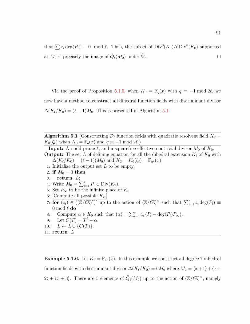
91

that∑zi deg(Pi) ≡ 0 mod `. Thus, the subset of Div0(K0)/`Div0(K0) supported

at M0 is precisely the image of Q`(M0) under Ψ.

Via the proof of Proposition 5.1.5, when K0 = Fq(x) with q ≡ −1 mod 2`, we

now have a method to construct all dihedral function fields with discriminant divisor

∆(K`/K0) = (`− 1)M0. This is presented in Algorithm 5.1.

Algorithm 5.1 (Constructing D` function fields with quadratic resolvent field K2 =K0(ζ`) when K0 = Fq(x) and q ≡ −1 mod 2`.)

Input: An odd prime `, and a squarefree effective nontrivial divisor M0 of K0.Output: The set L of defining equation for all the dihedral extension K` of K0 with

∆(K`/K0) = (`− 1)(M0) and K2 = K0(ζ`) = Fq2(x)1: Initialize the output set L to be empty.2: if M0 = 0 then3: return L;4: Write M0 =

∑ri=1 Pi ∈ Div(K2).

5: Set P∞ to be the infinite place of K0.6: [Compute all possible K`.]

7: for (zi) ∈ ((Z/`Z)∗)r

up to the action of (Z/`Z)× such that∑r

i=1 zi deg(Pi) ≡0 mod ` do

8: Compute α ∈ K0 such that (α) =∑r

i=1 zi (Pi − deg(Pi)P∞).9: Let C(T ) = T ` − α.10: L← L ∪ {C(T )}.11: return L

Example 5.1.6. Let K0 = F13(x). In this example we construct all degree 7 dihedral

function fields with discriminant divisor ∆(K`/K0) = 6M0 where M0 = 〈x+1〉+ 〈x+

2〉 + 〈x + 3〉. There are 5 elements of Q`(M0) up to the action of (Z/`Z)×, namely

92

the divisors

〈x+ 1〉+ 〈x+ 2〉+ 5〈x+ 3〉,

〈x+ 1〉+ 2〈x+ 2〉+ 4〈x+ 3〉,

〈x+ 1〉+ 3〈x+ 2〉+ 3〈x+ 3〉,

〈x+ 1〉+ 4〈x+ 2〉+ 2〈x+ 3〉,

〈x+ 1〉+ 5〈x+ 2〉+ 〈x+ 3〉.

These correspond to 5 dihedral fields with defining polynomials

T 7 − (x+ 1)(x+ 2)(x+ 3)5,

T 7 − (x+ 1)(x+ 2)2(x+ 3)4,

T 7 − (x+ 1)(x+ 2)3(x+ 3)3,

T 7 − (x+ 1)(x+ 2)4(x+ 3)2,

T 7 − (x+ 1)(x+ 2)5(x+ 3).

5.2 Construction with Quadratic Resolvent K2 when K2/K0

is geometric

In order to construct degree ` dihedral extensions with quadratic resolvent field K2/k2

when k2 does not contain the `-th roots of unity, we can adjoin the roots to k2 and

use the results of the last chapter to build the corresponding fields over K0(ζ), and

compute a fixed field to obtain a dihedral extension of K0. For the reasons discussed

at the beginning of last chapter, in this section we will assume that K2/K0 is a

93

geometric extension, i.e. that k2 = k0 . Under this assumption, we will present a

general Kummer theoretic algorithm for this case. The shortcomings of this general

algorithm will further motivate the restriction to the case when [k0(ζ`) : k0] = 2. In

Section 5.3 we will make that restriction and refine this general algorithm, resulting

in a much faster Kummer theoretic method for constructing dihedral function fields.

Recall that k/k is a cyclic Galois extension and hence so is K/K. Throughout,

let % denote a generator of Gal(K/K) that restricts to a generator of k/k. Now, if a

geometric extension K ′/K is Galois then so is K ′/K and Gal(K ′/K) ∼= Gal(K ′/K).

Furthermore, we have the following proposition:

Proposition 5.2.1. With the notation above, let K ′/K be a Galois extension of

function fields such that K ′ ∩ K = K. Then K ′/K is Galois and

Gal(K ′/K) ∼= Gal(K ′/K)×Gal(k/k).

Alternatively, if K ′/K is Galois and Gal(k′/k) is a normal subgroup of Gal(K ′/K)

then K ′/K is Galois.

Proof. The first statement follows directly from Proposition 14.21 of [17] since the

intersection K ∩ K ′ = K. The second statement follows directly from Theorem

2.2.3.

Now, when K2/K0 is geometric, we consider the diagram of fields given in Figure

5.1 that depicts the diagram of fields in Figure 2.1 and their constant field extensions

when adjoining ζ`.

Here, K2`/K0 is a dihedral Galois extension with quadratic resolvent K2 which is

a geometric extension of K0. Consequently, K2`/K0 is a dihedral Galois extension as

94

Figure 5.1: Adjoining `-th roots of unity to the diagram of a dihedral extension offunction fields.

K2`

K2` K`

2

K2

`〈σ〉

K`

2

K2

`〈σ〉

〈%〉

K0

2〈τ〉`

K0

2〈τ〉

`

well. We abuse notation by letting σ and τ denote the generators of Gal(K2`/K0)

that restrict to the generators σ, τ ∈ Gal(K2`, K0), respectively.

As K0 contains a primitive `-th root of unity, we can apply Algorithm 4.1 to

construct all fields K`/K0 with prescribed ramification. Then, if K2`/K0 is Galois

with Galois group D` × 〈%〉, we can take the fix field of % to obtain all dihedral

fields K`/K0 with the same ramification and correct quadratic resolvent. Moreover,

by Proposition 5.2.1, all dihedral extensions K`/K0 can be constructed in such a

manner. This is made precise in Algorithm 5.2.

Notice that the resulting function fields K` do indeed have discriminant divisor

∆(K`/K0) = `−12

(∆(K2/K0) +M) by Theorem 5.1.1.

This method is quite inefficient. One needs to compute the Galois group for each

field K2` and potentially a fixed field for each of these afterwards. In fact, when k0

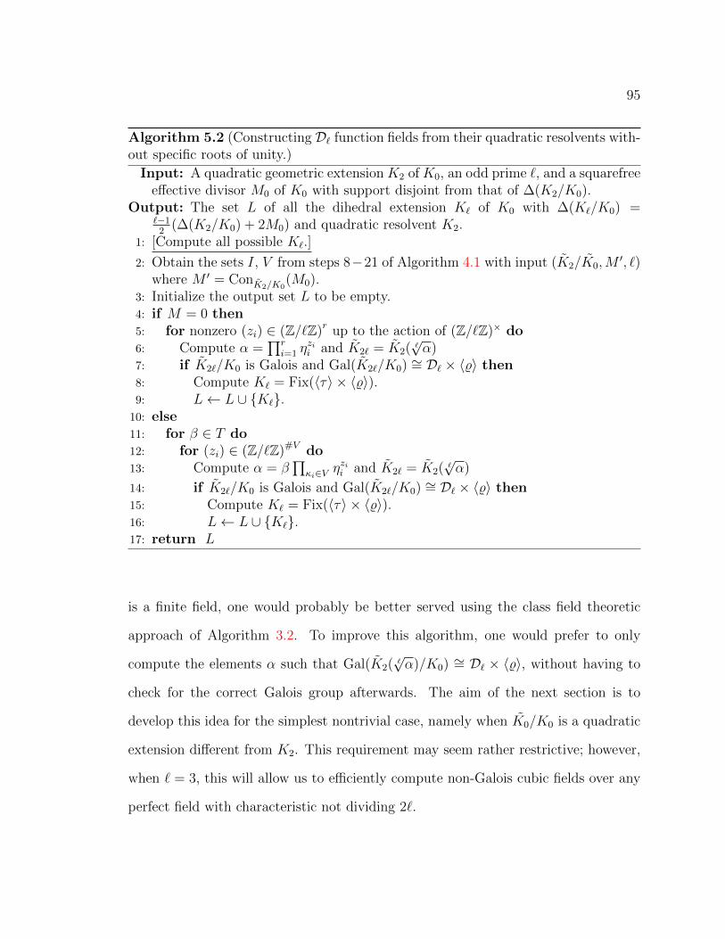
95

Algorithm 5.2 (Constructing D` function fields from their quadratic resolvents with-out specific roots of unity.)

Input: A quadratic geometric extension K2 of K0, an odd prime `, and a squarefreeeffective divisor M0 of K0 with support disjoint from that of ∆(K2/K0).

Output: The set L of all the dihedral extension K` of K0 with ∆(K`/K0) =`−1

2(∆(K2/K0) + 2M0) and quadratic resolvent K2.

1: [Compute all possible K`.]

2: Obtain the sets I, V from steps 8−21 of Algorithm 4.1 with input (K2/K0,M′, `)

where M ′ = ConK2/K0(M0).

3: Initialize the output set L to be empty.4: if M = 0 then5: for nonzero (zi) ∈ (Z/`Z)r up to the action of (Z/`Z)× do6: Compute α =

∏ri=1 η

zii and K2` = K2(

√α)

7: if K2`/K0 is Galois and Gal(K2`/K0) ∼= D` × 〈%〉 then8: Compute K` = Fix(〈τ〉 × 〈%〉).9: L← L ∪ {K`}.10: else11: for β ∈ T do12: for (zi) ∈ (Z/`Z)#V do13: Compute α = β

∏κi∈V η

zii and K2` = K2(

√α)

14: if K2`/K0 is Galois and Gal(K2`/K0) ∼= D` × 〈%〉 then15: Compute K` = Fix(〈τ〉 × 〈%〉).16: L← L ∪ {K`}.17: return L

is a finite field, one would probably be better served using the class field theoretic

approach of Algorithm 3.2. To improve this algorithm, one would prefer to only

compute the elements α such that Gal(K2(√α)/K0) ∼= D` × 〈%〉, without having to

check for the correct Galois group afterwards. The aim of the next section is to

develop this idea for the simplest nontrivial case, namely when K0/K0 is a quadratic

extension different from K2. This requirement may seem rather restrictive; however,

when ` = 3, this will allow us to efficiently compute non-Galois cubic fields over any

perfect field with characteristic not dividing 2`.

96

5.3 Construction when K2/K0 is geometric and [k0(ζ`) : k0] = 2

As mentioned, to produce an efficient Kummer theoretic method for constructing

dihedral fields, one would like to only compute the elements α ∈ K2 such that

Gal(K2(√α)/K0) ∼= D` × 〈%〉. In this section, we will achieve this when k2/k2 is

a quadratic extension. Thus, throughout this section we will assume that [k0(ζ`) :

k0] = [k2(ζ`) : k2] = 2, and thus K2 ∩ K0(ζ`) = K0. Moreover, for the reasons pre-

viously discussed, we will assume that K2/K0 is geometric. Recall, the case when

K2 = K0(ζ`) was covered in Section 5.1, and so we exclude this case from considera-

tion in this section.

To begin, consider the diagram of fields in Figure 5.2, which corresponds to Figure

5.1 to the case under consideration in this section. Here, we let K2 denote the twist

of K2, i.e. the other geometric subfield of K2/K0 different from K2. Notice that K2

is the subfield of K2 fixed by 〈%τ〉 = 〈τ%〉.

As mentioned, the goal of this section is to precisely determine the elements α ∈ K2

such that Gal(K2(√α)/K0) ∼= D` × 〈%〉. For any field extension K ′/K, let

N`(K ′/K) ={α ∈ K ′× \K× : NK′/K(α) ∈ (K×)`

}.

Then, we have the following theorem:

Theorem 5.3.1. The inclusion

Φ: N`(K2/K0)/(K×2 )` → N`(K2/K0)/(K×2 )`

is onto the subset of α(K×2 )` ∈ N`(K2/K0)/(K×2 )` such that K2(√α)/K0 is Galois

97

Figure 5.2: Adjoining `-th roots of unity to the diagram of a dihedral extension offunction fields when [K2(ζ`) : K2] = 2.

K2`

K2`

2

K`

2

K2

`〈σ〉

K`

2 2

K2

`

〈%〉

2

K0

2 〈τ〉`

K2

2〈%τ〉

K0

2` 2 2

with Gal(K2(√α)/K0) ∼= D` × 〈%〉.

Proof. Let α ∈ N`(K2/K0). First we show that α(K×2 )` is in the image of Φ if and

only if %τ(α)(K×2 )` = α(K×2 )`. As K2 is the fixed field of %τ in K2, %τ(α)(K×2 )` =

α(K×2 )` if α is the image of Φ. Conversely, suppose %τ(β)(K×2 )` = β(K×2 )` for some

β ∈ N`(K2/K0). Then %τ(β) = βκ` for some κ ∈ K2. Setting α = β/%τ(κ`), we

find that %τ(α) = α. Now, α ∈ N`(K2/K0) if and only if NK2/K0(α) = κ`0 for some

κ0 ∈ K0. By definition NK2/K0(α) = τ(α)α. However, the restriction of τ to K2 is the

nontrivial Galois automorphism of K2/K0, and thus NK2/K0(α) ∈ K0. Moreover, as

α ∈ N`(K2/K0), its norm is an `-th power, and thus there exists an element κ0 ∈ K0

such that NK2/K0(α) = NK2/K0

(α) = κ`0. Therefore, α(K×2 )` is in the image of Φ if

and only if %τ(α)(K×2 )` = α(K×2 )`.

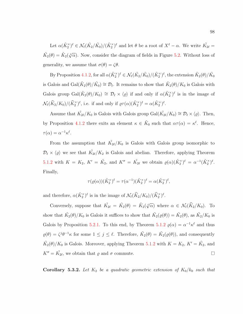
98

Let α(K×2 )` ∈ N`(K2/K0)/(K×2 )` and let θ be a root of X` − α. We write K2` =

K2(θ) = K2(√α). Now, consider the diagram of fields in Figure 5.2. Without loss of

generality, we assume that σ(θ) = ζθ.

By Proposition 4.1.2, for all α(K×2 )` ∈ N`(K2/K0)/(K×2 )`, the extension K2(θ)/K0

is Galois and Gal(K2(θ)/K0) ∼= D`. It remains to show that K2(θ)/K0 is Galois with

Galois group Gal(K2(θ)/K0) ∼= D` × 〈%〉 if and only if α(K×2 )` is in the image of

N`(K2/K0)/(K×2 )`, i.e. if and only if %τ(α)(K×2 )` = α(K×2 )`.

Assume that K2`/K0 is Galois with Galois group Gal(K2`/K0) ∼= D`×〈%〉. Then,

by Proposition 4.1.2 there exits an element κ ∈ K0 such that ατ(α) = κ`. Hence,

τ(α) = α−1κ`.

From the assumption that K2`/K0 is Galois with Galois group isomorphic to

D` × 〈%〉 we see that K2`/K2 is Galois and abelian. Therefore, applying Theorem

5.1.2 with K = K2, K ′ = K2, and K ′′ = K2` we obtain %(α)(K×2 )` = α−1(K×2 )`.

Finally,

τ(%(α))(K×2 )` = τ(α−1)(K×2 )` = α(K×2 )`,

and therefore, α(K×2 )` is in the image of N`(K2/K0)/(K×2 )`.

Conversely, suppose that K2` = K2(θ) = K2(√α) where α ∈ N`(K2/K0). To

show that K2(θ)/K0 is Galois it suffices to show that K2(%(θ)) = K2(θ), as K2/K0 is

Galois by Proposition 5.2.1. To this end, by Theorem 5.1.2 %(α) = α−1κ` and thus

%(θ) = ζjθ−1κ for some 1 ≤ j ≤ `. Therefore, K2(θ) = K2(%(θ)), and consequently

K2(θ)/K0 is Galois. Moreover, applying Theorem 5.1.2 with K = K2, K ′ = K2, and

K ′′ = K2`, we obtain that % and σ commute.

Corollary 5.3.2. Let K2 be a quadratic geometric extension of K0/k0 such that

99

[k0(ζ`) : k0] = 2. Then there is a one-to-one correspondence between dihedral function

fields K` with quadratic resolvent K2 and the set of nontrivial cyclic subgroups of

N`(K2/K0)/(K×2 )`.

Recall that the theory of `-virtual units presented in Section 4.1.2 is independent

of the presence of roots of unity in k2. So let

U`(K2) = {(α) + Prin(K2) ∩ `Div0(K2) : α ∈ N`(K2/K0)}.

Then we have the following corollary:

Corollary 5.3.3. Let K2 be a quadratic geometric extension of K0/k0 such that

[k0(ζ`) : k0] = 2. Then there is a one-to-one correspondence between dihedral function

fields K` with quadratic resolvent K2 and the set of nontrivial cyclic subgroups of

Pic0(K2)[`]× U`(K2).

From the above corollary, we can obtain an exact count for the number of dihedral

fields K` with quadratic resolvent K2, by replacing K2 with K2 in Theorem 4.1.12.

We spare the reader the nearly verbatim rewriting of Theorem 4.1.12 in this case.

However, as the theorem is constructive, in the next section we will use it to pro-

duce an algorithm for constructing dihedral function fields with a given discriminant

divisor.

5.4 Construction Algorithms when [k0(ζ`) : k0] = 2

In this section we present an algorithm for constructing all degree ` dihedral function

fields with a given discriminant divisor ∆ ∈ Div(K0/k0), when [k0(ζ`) : k0] = 2. We

first justify the use of Algorithm 4.1 to construct dihedral fields with given ramification

100

and a fixed quadratic resolvent K2 6= K0(ζ`), when [k0(ζ`) : k0] = 2. Then, under

Assumption COEFF, we combine this with Algorithm 5.1 to produce an algorithm for

constructing all dihedral fields of a given discriminant divisor when [k0(ζ`) : k0] = 2.

Thus, throughout this section assume that [k0(ζ`) : k0] = 2.

When K2/K0 is geometric, by Corollary 5.3.3, the function fields K2` such that

K2`/K0 is Galois with Galois group D` correspond to cyclic subgroups of the group

Pic0(K2)[`]×U`(K2). Let ∆ = `−12

∆(K2/K0) + (`− 1)M0. Let U`,M0(K2) denote the

subset of U`(K2) consisting of those classes

(α) + Prin(K2) ∩ `Div0(K2)

such that the reduced ramification divisor of α is equal to M0. Using the correspon-

dence of Corollary 5.3.3, the conjugacy classes of dihedral degree ` function fields with

discriminant divisor ∆(K`/K0) = ∆ and quadratic resolvent field K2 are in one-to-one

correspondence with the number of nontrivial cyclic subgroups of Pic0(K2)[`]×U`(K2)

that can be generated by elements (A,B) with B ∈ U`,M0(K2). Notice that Algorithm

4.1 computes all such pairs on input K2, `,M0.

Via Φ we can embed the set N`(K2/K0)/(K×2 )` into N`(K2/K0)/(K×2 )`. Then

with C`,κ(T ) as defined in Definition 4.1.13, Proposition 4.1.14 says that

C(T ) = C`,κ(T )− TrK2/K0(α) ∈ K0[T ]

is a defining polynomial of K`/K0. However, recall from the proof of Theorem 5.3.1

that if α(K×2 )` ∈ N`(K2/K0)/(K×2 )` then NK2/K0(α) = κ` ∈ (K×0 )`. Moreover,

as ρ|K2is the nontrivial Galois automorphism of K2/K0, TrK2/K0

(α) = TrK2/K0(α).

101

Therefore, C(T ) is defined over K0 and is thus invariant under ρ. Consequently, C(T )

is a defining equation for K`/K0 as well.

All told, on input K2, `,M0, Algorithm 4.1 produces all dihedral fields K` such

that ∆(K`/K0) = ∆ with quadratic resolvent field K2 when K2/K0 is geometric.

Combining this with Algorithm 5.1, we obtain Algorithm 5.3 (when [k0(ζ`) : k0] = 2

and under Assumption COEFF) which constructs all dihedral function fields K`/K0

with quadratic resolvent field K2 such that ∆(K`/K0) = `−12D + (`− 1)M0,

Algorithm 5.3 (Constructing all D` function fields with quadratic resolvent field K2

when [k0(ζ`) : k0] = 2)

Input: A quadratic extension K2/k2 of K0/k0 under Assumption COEFF, an oddprime `, and a squarefree effective divisor M0 of K0 coprime to ∆(K2/K0).

Output: The set L of defining equations for all the degree ` dihedral extensions K`

of K0 with ∆(K`/K0) = `−12D + (`− 1)M0.

1: [Compute all possible K`.]2: if ∆(K2/K0) = 0 then3: Get L from Algorithm 5.1 with input `,M0.4: else5: Get L from Algorithm 4.1 with input K2, `,M0.6: return L.

Example 5.4.1. Consider the rational function field F9(x) where F9 = F3(ω) and ω

is a root of T 2− T − 1. One can check that ω generates F×9 . In this example, we will

construct an degree 5 dihedral extension with M0 = 0. Let K2 and K2 be defined by

the equations

z2 = ωx(x− ω)(x− ω2)(x− ω3)(x− ω4),

y2 = x(x− ω)(x− ω2)(x− ω3)(x− ω4),

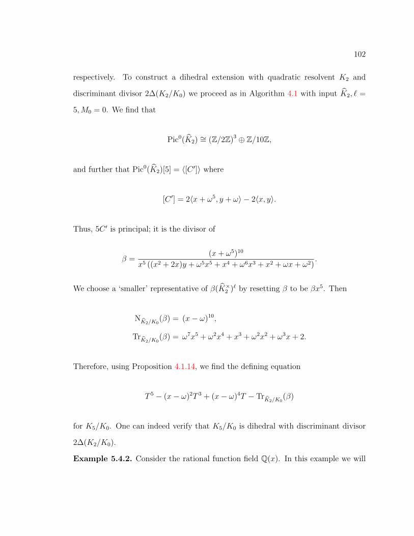
102

respectively. To construct a dihedral extension with quadratic resolvent K2 and

discriminant divisor 2∆(K2/K0) we proceed as in Algorithm 4.1 with input K2, ` =

5,M0 = 0. We find that

Pic0(K2) ∼= (Z/2Z)3 ⊕ Z/10Z,

and further that Pic0(K2)[5] = 〈[C ′]〉 where

[C ′] = 2〈x+ ω5, y + ω〉 − 2〈x, y〉.

Thus, 5C ′ is principal; it is the divisor of

β =(x+ ω5)10

x5 ((x2 + 2x)y + ω5x5 + x4 + ω6x3 + x2 + ωx+ ω2).

We choose a ‘smaller’ representative of β(K×2 )` by resetting β to be βx5. Then

NK2/K0(β) = (x− ω)10,

TrK2/K0(β) = ω7x5 + ω2x4 + x3 + ω2x2 + ω3x+ 2.

Therefore, using Proposition 4.1.14, we find the defining equation

T 5 − (x− ω)2T 3 + (x− ω)4T − TrK2/K0(β)

for K5/K0. One can indeed verify that K5/K0 is dihedral with discriminant divisor

2∆(K2/K0).

Example 5.4.2. Consider the rational function field Q(x). In this example we will

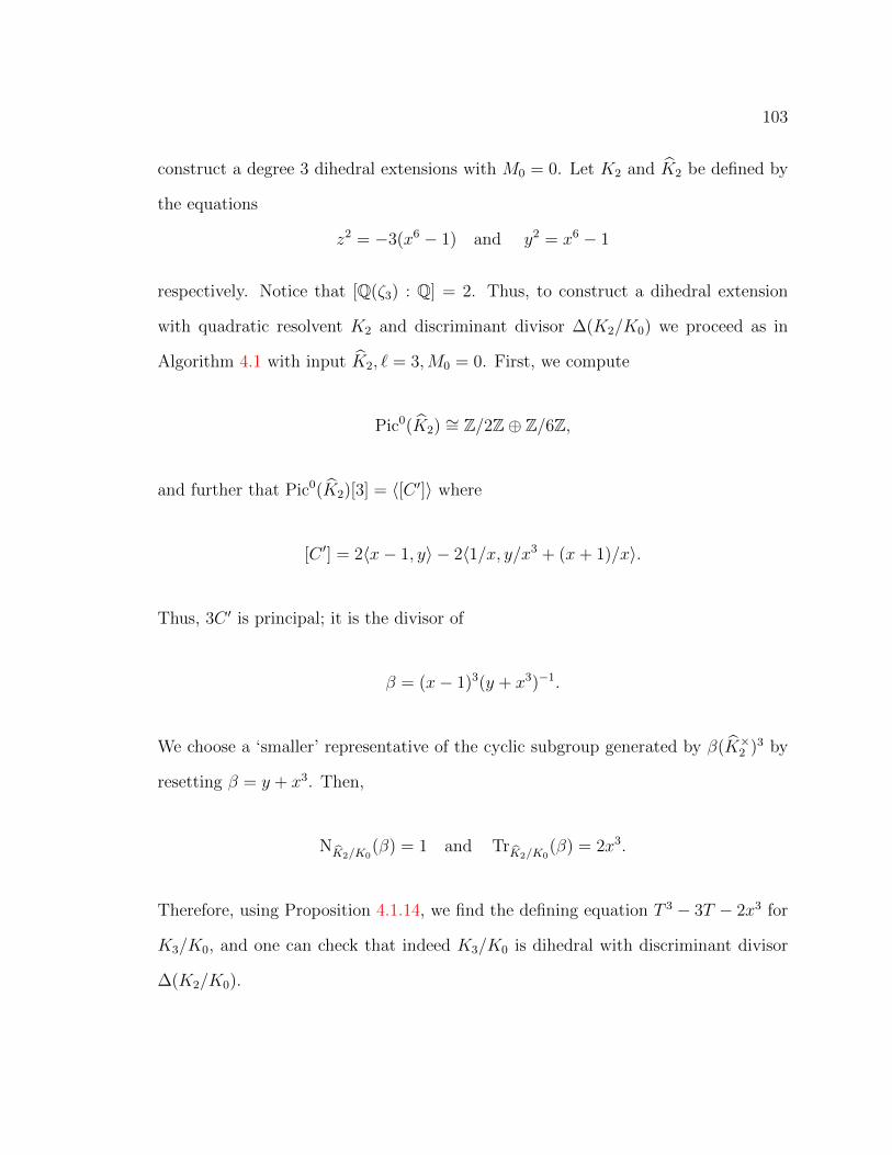
103

construct a degree 3 dihedral extensions with M0 = 0. Let K2 and K2 be defined by

the equations

z2 = −3(x6 − 1) and y2 = x6 − 1

respectively. Notice that [Q(ζ3) : Q] = 2. Thus, to construct a dihedral extension

with quadratic resolvent K2 and discriminant divisor ∆(K2/K0) we proceed as in

Algorithm 4.1 with input K2, ` = 3,M0 = 0. First, we compute

Pic0(K2) ∼= Z/2Z⊕ Z/6Z,

and further that Pic0(K2)[3] = 〈[C ′]〉 where

[C ′] = 2〈x− 1, y〉 − 2〈1/x, y/x3 + (x+ 1)/x〉.

Thus, 3C ′ is principal; it is the divisor of

β = (x− 1)3(y + x3)−1.

We choose a ‘smaller’ representative of the cyclic subgroup generated by β(K×2 )3 by

resetting β = y + x3. Then,

NK2/K0(β) = 1 and TrK2/K0

(β) = 2x3.

Therefore, using Proposition 4.1.14, we find the defining equation T 3 − 3T − 2x3 for

K3/K0, and one can check that indeed K3/K0 is dihedral with discriminant divisor

∆(K2/K0).

104

Under Assumption COEFF, when [k0(ζ`) : k0] = 2, we now combine Algorithms

5.1 and 4.1 to create an algorithm that outputs all dihedral degree ` function fields

with a given discriminant divisor. This is presented in Algorithm 5.4.

Algorithm 5.4 (Constructing all D` function fields over K0/k0 from their divisorswhen [k0(ζ`) : k0] = 2

Input: An odd prime ` and squarefree effective divisors D and M0 of K0 withdisjoint support, where K0 = Fq(x) when D = 0.

Output: The set L of defining equations for all the degree ` dihedral extensions K`

of K0 with ∆(K`/K0) = `−12D + (`− 1)M0.

1: if deg(D) is even then2: Construct a quadratic field K2 with discriminant divisor D.3: else4: return “D is not a quadratic discriminant divisor”.5: if D = 0 then6: Get L from Algorithm 5.1 with input `,M0.7: else8: Construct the quadratic twist K2 of K2.9: if M0 6= 0 then10: Pick P ∈ Supp(M0).11: if P splits in K2 then12: Get L from Algorithm 4.1 with input K2, `,M0.13: else14: Get L from Algorithm 4.1 with input K2, `,M0.15: else16: Get L1 from Algorithm 4.1 with input K2, `,M0.17: Get L2 from Algorithm 4.1 with input K2, `,M0.18: Set L← L1 ∪ L2.19: return L.

Example 5.4.3. Returning to Examples 5.1.6, and 5.4.2 we find the following:

1. On input D = 0 and M0 = 〈x+ 1〉+ 〈x+ 2〉+ 〈x+ 3〉 as in from Example 5.1.6,

the output of Algorithm 4.2 is the five fields K5 found in Example 5.1.6.

2. On input ∆(K2/K0) from Example 5.4.2, M0 = 0, and ` = 3, the output

105

of Algorithm 4.2 is the field K3 found in Example 5.4.2 as Pic0(K2) has no

nontrivial 3-torsion.

So using the algorithms of the last chapter we are now able to construct dihe-

dral function fields with prescribed ramification when [k2(ζ`) : k2] = 2. Notice that

this allows us to produce complete tables of cubic fields when k is a finite field of

characteristic greater than 3. We will explore this further in the next chapter.

106

Chapter 6

Numerical Results and Tabulation

Techniques

In this chapter, we present a method to efficiently tabulate all degree ` dihedral func-

tion fields whose discriminant divisors have degree up to a given bound B when k0 is

a finite field Fq and q is coprime to 2`. Instead of simply iterating one of the construc-

tion methods of the previous chapters, we are able to exact improvements from using

the automorphism group of the field K0. After describing this improvement, we dis-

cuss the numerical results from this implementation when q ≡ ±1 mod 2`. We will

see that in all the instances we implemented, the Kummer theoretic approach per-

forms better than the one using class field theory. Consequently, we use the Kummer

theoretic approach in our tabulation algorithm to construct complete lists of dihedral

fields up to various bounds B for several values of `. These lists are then compared

to relevant asymptotic formulas and explicit counting results.

The tabulation technique we will present is my own work and was first presented

in [42] for the case that q ≡ 1 mod 2`. In [42], we also compared the same tabulation

results to the relevant asymptotics in this case. Theorem 6.2.3, which provides an

explicit count for the number of degree ` dihedral function fields of the smallest degree

bound when q ≡ 1 mod 2`, was also originally presented in [42] and is due to Everett

107

Howe. However, we will extend that result to include the case when q ≡ −1 mod 2`.

Throughout this chapter k0 with be a finite field Fq with odd characteristic differ-

ent from `.

6.1 Tabulation Method

Algorithms 4.1, 3.2, and 5.3 construct all degree ` dihedral function fields with a given

discriminant divisor and fixed quadratic resolvent field; by iterating either of these

algorithms, we obtain a procedure for tabulating all degree ` dihedral function fields

whose discriminant divisor has degree up to some fixed input bound B ≥ 0. However,

in this context, we can use the automorphism group of K0 to significantly reduce the

number of quadratic function fields that need to be considered.

As we will see in the next section, Algorithm 4.1 performs better than Algorithm

3.2, and hence we tabulated dihedral function fields primarily using that algorithm.

However, we will present our tabulation method in full generality; we will only assume

q is odd and not a power of `.

Recall that Aut(K0) = Aut(Fq(x)) is isomorphic to PGL(2, q), the group of frac-

tional linear transformations of x over Fq. The group Aut(K0) also acts on the

set of extension fields Ki of K0, and for every φ ∈ Aut(K0) we have φ(∆(Ki/K0)) =

∆(φ(Ki)/K0). Therefore, instead of applying Algorithm 4.1 to all suitable K2 and M0,

we only need to consider a representative from each orbit of Aut(K0) acting on the set

of suitable quadratic function fields K2. Moreover, for each such field K2 we need only

consider representatives of the action of the stabilizer Stab(K2) ⊆ PGL(2, q) on the

set of suitable M0. After constructing all dihedral fields K` with quadratic resolvent

fields K2 from the set above, we then reapply the group of PGL(2, q)-automorphisms

108

to the set of fields K` (modulo their stabilizers) to obtain the complete list of exten-

sions K`/K0. These ideas are captured in Algorithms 6.1, 6.2, and 6.3.

We will let P (q, `, B, h) denote the set of nonconstant squarefree polynomials f ∈

Fq[x] whose degrees satisfy ddeg(f)/2e ≤ b2B/(`− 1)c and whose leading coefficient

is either 1 or a fixed nonsquare h in Fq. Algorithm 6.1 finds orbit representatives for

the set of quadratic function fields whose discriminant divisors are of degree at most

2B/(`− 1).

Algorithm 6.1 Constructing a list of PGL(2, q)-orbit representatives for quadraticfunction fields of bounded discriminant

Input: A nonnegative integer B, an odd prime `, and an odd prime power q 6≡0 mod ` and a primitive element h of Fq.

Output: A set R′B of all pairs (f, Sf ) such that f ∈ P (q, `, B, h), each Sf is thePGL(2, q)-stabilizer of the class of f in K×0 /(K

×0 )2, and such that every quadratic

extension K2 of K0 with deg ∆(K2/K0) ≤ 2B/(`− 1) has exactly one PGL(2, q)-orbit representative in the collection of fields defined by the f .

1: Initialize R′B ← {(h,PGL(2, q))}.2: Set L(f)← 0 for all f ∈ P (q, `, B, h).3: for f ∈ P (q, `, B, h) do4: if L(f) = 0 then5: for φ = ax+b

cx+d∈ PGL(2, q) do

6: f1(x)← (cx+ d)2d(deg f)/2ef(φ(x)).7: if the leading coefficient m of f1 is a square then8: Replace f1 with f1/m9: else10: Replace f1 with hf1/m.11: L(f1)← 1.12: if f1 = f then13: Sf ← Sf ∪ {φ}.14: R′B ← R′B ∪ {(f, Sf )}.15: S ← ∅.16: Return R′B.

Recall that every quadratic function field K2 can be expressed as K0(y), where

109

y2 is equal to either a nonsquare in Fq or a squarefree polynomial f(x) ∈ Fq[x] of

degree 2g + 1 or 2g + 2, where g is the genus of K2. In the former case, K2 is fixed

under PGL(2, q). In the latter case, the action of φ ∈ PGL(2, q) on K2 does not

necessarily preserve the degree of f(x), but φ(K2) has the same genus as K2; in fact,

the discriminant divisors of K2 and φ(K2) have the same degree, namely 2g+2. Thus,

fields in the same PGL(2, q)-orbit have discriminant divisors of the same degree.

Algorithm 6.2 constructs minimal polynomials for all dihedral function fields with

discriminant divisors `−12

∆K2 + (`− 1)M0 for all suitable M0 for each representative

K2 obtained from Algorithm 6.1.

Finally, Algorithm 6.3 reapplies Aut(K) to each of the minimal polynomials con-

structed in Algorithm 6.2 to obtain the full list of degree ` dihedral function fields

whose discriminant divisor has degree bounded by B.

The technique of utilizing Aut(Fq(x)) does result in a significant reduction in run

time versus the naive method of iteration for tabulation. This can be seen in Tables

6.2 and 6.3. This and other numerical results are discussed in the following section.

110

Algorithm 6.2 Tabulating PGL(2, q)-orbit representatives of dihedral function fieldswith bounded discriminant

Input: A nonnegative integer B, an odd prime `, an odd prime power q 6≡ 0 mod `,and the set R′B computed by Algorithm 6.1 on input B, `, q, h.

Output: A set RB of triples (L2,∆, S∆) such that each ∆ is an effective divisor ofK of degree at most B, the group S∆ is the PGL(2, q)-stabilizer of ∆, the setL2 consists of defining equations for the PGL(2, q)-orbit representatives of D`extensions of K0 with discriminant divisor ∆.

1: Initialize RB ← ∅.2: for (f, Sf ) ∈ R′B do3: Construct K2 = K0(x)[y]/〈y2 − f〉 and compute ∆(K2/K0).4: Compute B′ = bB/(`− 1)− (deg(∆(K2/K0)))/2c.5: Initialize M← ∅; eventually, M will contain all effective squarefree divisors of

K0 with support disjoint from ∆(K2/K0) and degree at most B′.6: Compute lists Lj = {P ∈ P(K0)\Supp ∆(K2/K0) : degP = j} for 1 ≤ j ≤ B′.

7: for i from 0 to B′ and for every partition n = [n1, .., nr] of i do8: Generate the set Wn = {

∑rk=1 Pk : Pk ∈ Lnk

}.9: M←M ∪Wn.10: Compute the set MS of all pairs (M0, S∆) where each M0 ∈M is a unique orbit

representative of Sf acting on M and S∆ is the stabilizer of M0 in Sf .11: for (M0, S∆) ∈MS do12: Get L2 from Algorithm 3.2 (or 4.1 if q ≡ 1 mod ` or 5.3 if q ≡ −1 mod `) on

input (K2, `,M0).13: Compute ∆ = `−1

2∆K2 + (`− 1)M0.

14: RB ← RB ∪ {(L2,∆, S∆)}.15: Return RB.

Algorithm 6.3 Tabulating the full list of dihedral function fields with boundeddiscriminant

Input: A nonnegative integer B, an odd prime `, an odd prime power q 6≡ 0 mod `,and the set RB computed by Algorithm 6.2 on input B, `, q.

Output: A set LB of defining equations for all the dihedral extensions K` of K withdeg ∆K`

≤ B.1: Initialize LB ← ∅.2: for (L,∆, S∆) ∈ RB do3: for all distinct coset representatives φ of PGL(2, q)/S∆ and all C(X) ∈ L do4: Set LB ← LB ∪ {(φ(C(X)), φ(∆))}.5: Return LB.

111

6.2 Implementations and Numerical Results

All computations were carried out using Magma on one core of a 2GHz Intel Xeon

X7550, with 64GB of available RAM. For ease of presentation all the tables of data

are gathered together at the end of this chapter in Section 6.3. Throughout, the

column headed K2/∼ gives the number of quadratic function fields generated by

Algorithm 6.1. The number of function fields constructed by Algorithm 6.2 is given

in the column headed K`/∼, and the total number of nonconjugate dihedral degree `

function fields whose discriminant divisor has degree at most B is listed in the column

headed K`.

We begin by comparing the Kummer theoretic approach of Algorithm 4.1 to the

class field approach of Algorithm 3.2. We ran Algorithm 6.2 with various inputs for the

two cases when q ≡ ±1 mod 2` and recorded our findings in Table 6.1. Both methods

produced the same number of fields (instilling confidence in our implementation), but

Algorithm 4.1 performs this computation in less time than Algorithm 3.2; the ratio

R0 of the two run times is seen in the last column of Table 6.1.

Notice that the improvement factorR0 of Algorithm 3.2 over Algorithm 4.1 is much

more pronounced when q ≡ −1 mod `. In this case, approximately 75% of the run

time is spent preforming Magma’s built-in algorithms to find defining equations for the

fields K2`/K2, while only approximaltely 25% of the run time is spent on this process

when q ≡ 1 mod `. This disparity is due to the fact that Magma’s method for finding

a defining equation of K2`/K2 utilizes Kummer Theory and Theorem 3.1.5 explicitly.

Thus, calculations in Algorithm 3.2 are performed in the extension field K2(ζ`), while

Algorithm 4.2 does not extend the constant field and performs calculations in K2.

This also seems to explain why for a fixed B and ` the improvement factor R0 grows

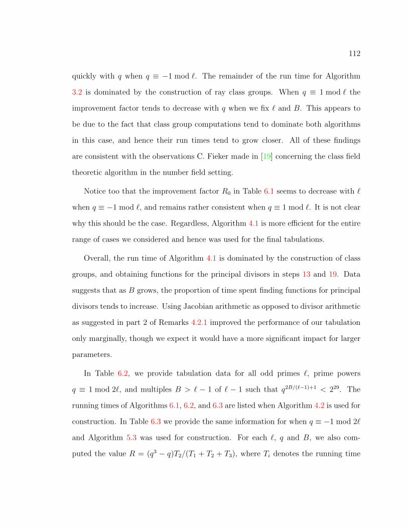
112

quickly with q when q ≡ −1 mod `. The remainder of the run time for Algorithm

3.2 is dominated by the construction of ray class groups. When q ≡ 1 mod ` the

improvement factor tends to decrease with q when we fix ` and B. This appears to

be due to the fact that class group computations tend to dominate both algorithms

in this case, and hence their run times tend to grow closer. All of these findings

are consistent with the observations C. Fieker made in [19] concerning the class field

theoretic algorithm in the number field setting.

Notice too that the improvement factor R0 in Table 6.1 seems to decrease with `

when q ≡ −1 mod `, and remains rather consistent when q ≡ 1 mod `. It is not clear

why this should be the case. Regardless, Algorithm 4.1 is more efficient for the entire

range of cases we considered and hence was used for the final tabulations.

Overall, the run time of Algorithm 4.1 is dominated by the construction of class

groups, and obtaining functions for the principal divisors in steps 13 and 19. Data

suggests that as B grows, the proportion of time spent finding functions for principal

divisors tends to increase. Using Jacobian arithmetic as opposed to divisor arithmetic

as suggested in part 2 of Remarks 4.2.1 improved the performance of our tabulation

only marginally, though we expect it would have a more significant impact for larger

parameters.

In Table 6.2, we provide tabulation data for all odd primes `, prime powers

q ≡ 1 mod 2`, and multiples B > ` − 1 of ` − 1 such that q2B/(`−1)+1 < 229. The

running times of Algorithms 6.1, 6.2, and 6.3 are listed when Algorithm 4.2 is used for

construction. In Table 6.3 we provide the same information for when q ≡ −1 mod 2`

and Algorithm 5.3 was used for construction. For each `, q and B, we also com-

puted the value R = (q3 − q)T2/(T1 + T2 + T3), where Ti denotes the running time

113

of Algorithm 6.i for i = 1, 2, 3. The quantity R estimates the improvement factor

obtained by our tabulation method relative to simply iterating Algorithm 4.1, or 5.3,

respectively, over all possible quadratic function fields without using the PGL(2, q)

action.

Notice that the improvement factor R is highly varied. For fixed ` and q, R tends

to decrease as B increases although the improvement still remains significant. Why

this decrease occurs is unclear; it may be due to the fact that R is not a sufficiently

refined estimate for the actual running time improvement.

Examining the asymptotic complexity of our tabulation method, we recall that

the asymptotic run time of tabulation is dominated by the repeated computation of

the divisor class groups in Algorithm 4.2. The method implemented in Magma for

computing the divisor class group of a function field of genus g over Fq is that of Hess

[23]. It is a sub-exponential probabilistic index calculus algorithm with expected run

time exp(√

log qg log log qg)c+o(1) for some explicit positive constant c as g →∞.

We need to apply Algorithm 6.1 essentially qB−3 times to quadratic function fields

of genus at most (B − 2)/2. Combining these results gives an asymptotic complexity

of qB exp(√

log qB log log qB)c+o(1) as B →∞. However, as we only ran our algorithm

with small values of B, this run time analysis is of limited value. Moreover in terms

of asymptotic complexity, performing Algorithms 6.1 and 6.3 have no benefit over the

naive tabulation method, even though they are extremely valuable in practice.

6.2.1 Asymptotic Comparison when ` = 3

In the case when ` = 3, our algorithm tabulates all non-Galois cubic function fields

up to a given degree bound on the discriminant divisor over any finite field with

114

characteristic greater than 3. Galois cubics are not difficult to count, so we can find

the total number of cubic extensions of K whose discriminant divisors have degree at

most some fixed bound. To illustrate the counting of Galois cubic fields, consider the

following example:

Example 6.2.1. In this example we compute the number of Galois extension K3/K0

with deg(∆(K3/K0)) = 4 and deg(∆(K3/K0)) = 6 when q ≡ 1 mod 3. By The-

orem 5.1.2, the number of geometric extensions equals the number of representa-

tives of the cyclic subgroups of K×0 /(K×0 )3 such that

∑P∈Supp((α)) deg(P ) = 2, and

3, respectively. As |F×q /F3q| = 3, and Pic0(K0) = 0, for each coset representative

D of Div0(K0)/3 Div0(K0), there are 3 choices of α ∈ K×0 /(K×0 )3 such that (α) =

D + 3 Div(K0). Moreover, as α and α2 correspond to isomorphic cyclic subgroups of

K×0 /(K×0 )3, the number of Galois extensions K3/K0 with deg(∆(K3/K0)) = 4 and

deg(∆(K3/K0)) = 6 is 3 times the number of cosets in Div0(K0)/3 Div(K0) up to

multiplication by 2, whose support has degree 4, or 6 respectively.

By the division algorithm, can write each coset D + 3 Div0(K0) uniquely as

D1 + 2D2 + 3 Div0(K0) for some effective coprime divisors D1, D2 ∈ Div(K0), where

deg(D1) + 2 deg(D2) ≡ 0 mod 3. Thus we need only count the number of possibilities

for D1 and D2 such that deg(D1 + D2) = 4 and 6, respectively, up to multiplication

by 2.

B = 4: Here the only possibility is deg(D1) = deg(D2) = 1. There are 3(q + 1)q/2

distinct cyclic cubic fields.

B = 6: Here the only possibility is deg(D1) = 2 and deg(D2) = 1. When D1 is a place

of degree 2 there are (q+1)(q2−q)/2 distinct choices for D, and when when D1

is the sum of two places of degree 1 there are q(q + 1)(q − 1)/6 distinct choices

115

for D. Therefore there are 2q(q + 1)(q− 1) cyclic cubic extensions K3/K0 with

deg(∆((K3/K0)) = 6.

When q ≡ −1 mod 3, the number of Galois extensions can be counted with similar

formulas to those above. We, however, simply counted such extensions taking 3 times

the result of Algorithm 4.2 with input (Fq2(x), B, 3). Notice that by Theorem 5.1.2,

Algorithm 4.2 conveniently produces abelian extensions with this input.

We now compare our total counts to the asymptotic predictions. A result of

Datskovsky and Wright [14, Theorem I.1] provides an asymptotic formula for the

number of cubic extensions who have discriminant divisors of degree at most B:

limB→∞B even

q−B∑K3/K0

deg ∆(K3/K0)≤B

1 =q3

(q2 − 1)(q − 1)ζK0(3)=q2 + q + 1

q2. (6.1)

(Note that the term 2 log q in [14, Theorem I.1] should be simply log q.)

In Table 6.4 we compare this asymptotic expression to our actual computations.

For each q and B listed in the first two columns, the entry in column 5 gives the total

number of cubic extensions of Fq(x) with discriminant divisor of degree at most B,

broken down into the number of non-Galois extensions (column 3) and Galois exten-

sions (column 4). Column 6 gives the estimate from equation (6.1), and column 7

gives the ratio R3 of the estimate to the actual values.

As in the number field setting, the leading term of the asymptotic expression

overestimates the actual number of cubic function fields, which leads us to believe

that the secondary term has a negative coefficient. An explicit computation of this

secondary term is currently underway by Yongqiang Zhao [44].

Remark 6.2.2. Notice too that in all cases we computed, the ratio R3 for B = 8 is

116

larger than that for B = 6, which in turn is larger than that for B = 4. However, the

result of [14] says that R3 should tend to 1 as B tends to infinity. It is interesting to

note that when q = 5 (the only case were we where able to fully tabulate when B = 10)

the ratio R3 is closer to 1 than the case when B = 8. One possible explanation for

this is that the number of cubic fields with M0 6= 0 for B < 10 is a relatively smaller

proportion than when B ≥ 10.

6.2.2 Explicit Formulas for B = 2(`− 1)

In this section we give an explicit formula for the number of D` extensions whose

discriminant divisor has degree 2(` − 1). This result was first presented in [42] and

is originally due to to Everett Howe. Here, we will extend his formula to the case

q ≡ −1 mod 2`.

Notice that by Corollary 3.2.4 there are no D` extensions whose discriminant

divisor has degree less than 2(`− 1). On the other hand, there do exist D` extensions

with discriminant divisor of degree 2(`− 1), as seen in the following theorem:

Theorem 6.2.3 ([42] Thm 5.1). Let ` be an odd prime and let q be a prime power

with q ≡ 1 mod 2`. For every nonnegative even integer d, let Nd be the number of

D` extensions of K0 whose quadratic resolvents have discriminant divisors of degree

d and whose discriminant divisors have degree 2(`− 1). Let X be the modular curve

117

X1(`). Then

Nd

q3 − q=

1

2q + 2if d = 0,

1 if d = 2,

−2 +2#X(Fq)`− 1

if d = 4,

0 otherwise.

When q ≡ −1 mod 2`, we obtain a similar result, where only the case d = 0 is

different. Indeed, we have the following theorem:

Theorem 6.2.4. Let ` be an odd prime and let q be a prime power with q ≡ −1 mod

2`. For every nonnegative even integer d, let Nd be the number of D` extensions

of K0 whose quadratic resolvents have discriminant divisors of degree d and whose

discriminant divisors have degree 2(`− 1). Let X be the modular curve X1(`). Then

Nd

q3 − q=

1

2q − 2if d = 0,

1 if d = 2,

−2 +2#X(Fq)`− 1

if d = 4,

0 otherwise.

Proof. For the case that d = 0, by Theorem 5.1.2, we see that non-Galois extensions

when q ≡ −1 mod 2` correspond to the coset representatives α of the cyclic subgroups

of K×0 /(K×0 )3 such that

∑P∈Supp((α)) deg(P ) = 2. As we saw in Example 6.2.1, there

are q(q + 1)/2 such representatives.

118

The case that d = 2 follows exactly as in [42] replacing K2 with K2.

In the case that d = 4, we obtain from the proof of Theorem 5.1 in [42] that

N4

# PGL(2, q)=

2

`− 1

∑(E,P )/∼=

1

# Aut(E,P ). (6.2)

where the sum is over isomorphism classes of pairs (E,P ), with E an an elliptic curve

over Fq and P a nonzero `-torsion point in E(Fq); two such pairs (E1, P1) and (E2, P2)

are isomorphic to one another when there is an isomorphism E1 → E2 that takes P1

to P2. The automorphism group of a pair (E,P ) consists of the automorphisms of E

(as an elliptic curve) that fix P .

From [24, Prop 3.3, p. 240] and [24, Prop 2.3, p. 233], Howe then shows that

∑(E,P )/∼=

1

# Aut(E,P )= #X(Fq)− c,

where c is the number of Fq-rational cusps on X. Since Fq2 contains the `-th roots of

unity, all of the `− 1 geometric cusps of X are defined over Fq [36, Theorem 1.3.1(b),

p. 12], so we have c = ` − 1. Combining this with equation (6.2) gives the formula

for N4 stated in the theorem.

For ` = 3, 5, and 7, the modular curve X1(`) has genus 0, so for these values of `

the formula for N4 simplifies to

N4

q3 − q=

2(q − `+ 2)

`− 1.

In these cases, our tabulation data verifies this result, further supporting the correct-

ness of our implementation. We note that equations for X1(`) for larger values of `

119

are also known [38].

Notice that the values of these formulas agree with the data in Tables 6.2 and 6.3.

Remark 6.2.5. Note that for B = 4, Theorems 6.2.3 and 6.2.4 give explicit formulas

for the number of cubic extensions when q is odd and q ≡ ±1 mod 3:

1. When q ≡ 1 mod 3, by Theorem 6.2.3, the number of non-Galois extensions is

(q3 − q)(

1

2q + 2+ 1 + (q − 1)

)= q4 − q2 + q

2,

and by Example 6.2.1, and including Fq3 , the number of Galois extensions is

(3q2 + 3q + 2)/2, so the total number of cubic extension is q4 + q2 + q + 1. It

follows that for B = 4 the ratio in column 7 of Table 6.4 is equal to

1 +q3 − q − 1

q4 + q2 + q + 1.

2. When q ≡ −1 mod 3, by Theorem 6.2.4, the number of non-Galois extensions

is

(q3 − q)(

1

2q − 2+ 1 + (q − 1)

)= q4 − q2 − q

2,

and the number of Galois extensions is (3q2− 3q+ 2)/2, so the total number of

cubic extension is q4 +q2−q+1. It follows that for B = 4 the ratio in column 7

of Table 6.4 is equal to

1 +q3 + q − 1

q4 + q2 − q + 1.

Notice that the secondary terms of the above ratios both have degree −1 in q

120

6.3 Tables of Numerical Data

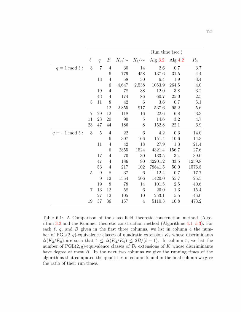
121

Run time (sec.)

` q B K2/∼ K`/∼ Alg 3.2 Alg 4.2 R0

q ≡ 1 mod ` : 3 7 4 30 14 2.6 0.7 3.76 779 458 137.6 31.5 4.4

13 4 58 30 6.4 1.9 3.46 4,647 2,538 1053.9 264.5 4.0

19 4 78 38 12.0 3.8 3.243 4 174 86 60.7 25.0 2.5

5 11 8 42 6 3.6 0.7 5.112 2,855 917 537.6 95.2 5.6

7 29 12 118 16 22.6 6.8 3.311 23 20 90 5 14.6 3.2 4.723 47 44 186 8 152.8 22.1 6.9

q ≡ −1 mod ` : 3 5 4 22 6 4.2 0.3 14.06 307 166 151.4 10.6 14.3

11 4 42 18 27.9 1.3 21.46 2855 1524 4321.4 156.7 27.6

17 4 70 30 133.5 3.4 39.047 4 186 90 42201.2 33.5 1259.853 4 217 102 78841.5 50.0 1576.8

5 9 8 37 6 12.4 0.7 17.79 12 1554 506 1420.0 55.7 25.5

19 8 78 14 101.5 2.5 40.67 13 12 58 6 20.0 1.3 15.4

27 12 105 10 253.1 5.5 46.019 37 36 157 4 5110.3 10.8 473.2

Table 6.1: A Comparison of the class field theoretic construction method (Algo-rithm 3.2 and the Kummer theoretic construction method (Algorithms 4.1, 5.3). Foreach `, q, and B given in the first three columns, we list in column 4 the num-ber of PGL(2, q)-equivalence classes of quadratic extension K2 whose discriminants∆(K2/K0) are such that 4 ≤ ∆(K2/K0) ≤ 2B/(` − 1). In column 5, we list thenumber of PGL(2, q)-equivalence classes of D` extensions of K whose discriminantshave degree at most B. In the next two columns we give the running times of thealgorithms that computed the quantities in column 5, and in the final column we givethe ratio of their run times.

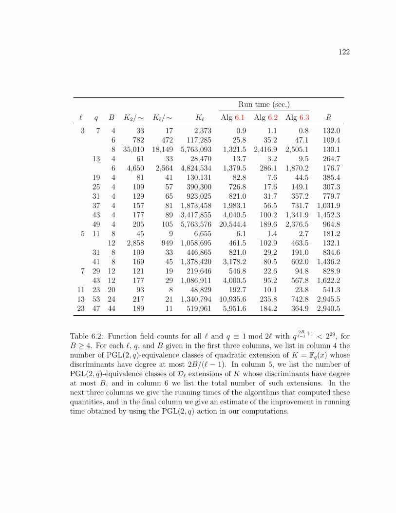
122

Run time (sec.)

` q B K2/∼ K`/∼ K` Alg 6.1 Alg 6.2 Alg 6.3 R

3 7 4 33 17 2,373 0.9 1.1 0.8 132.06 782 472 117,285 25.8 35.2 47.1 109.48 35,010 18,149 5,763,093 1,321.5 2,416.9 2,505.1 130.1

13 4 61 33 28,470 13.7 3.2 9.5 264.76 4,650 2,564 4,824,534 1,379.5 286.1 1,870.2 176.7

19 4 81 41 130,131 82.8 7.6 44.5 385.425 4 109 57 390,300 726.8 17.6 149.1 307.331 4 129 65 923,025 821.0 31.7 357.2 779.737 4 157 81 1,873,458 1,983.1 56.5 731.7 1,031.943 4 177 89 3,417,855 4,040.5 100.2 1,341.9 1,452.349 4 205 105 5,763,576 20,544.4 189.6 2,376.5 964.8

5 11 8 45 9 6,655 6.1 1.4 2.7 181.212 2,858 949 1,058,695 461.5 102.9 463.5 132.1

31 8 109 33 446,865 821.0 29.2 191.0 834.641 8 169 45 1,378,420 3,178.2 80.5 602.0 1,436.2

7 29 12 121 19 219,646 546.8 22.6 94.8 828.943 12 177 29 1,086,911 4,000.5 95.2 567.8 1,622.2

11 23 20 93 8 48,829 192.7 10.1 23.8 541.313 53 24 217 21 1,340,794 10,935.6 235.8 742.8 2,945.523 47 44 189 11 519,961 5,951.6 184.2 364.9 2,940.5

Table 6.2: Function field counts for all ` and q ≡ 1 mod 2` with q2B`−1

+1 < 229, forB ≥ 4. For each `, q, and B given in the first three columns, we list in column 4 thenumber of PGL(2, q)-equivalence classes of quadratic extension of K = Fq(x) whosediscriminants have degree at most 2B/(` − 1). In column 5, we list the number ofPGL(2, q)-equivalence classes of D` extensions of K whose discriminants have degreeat most B, and in column 6 we list the total number of such extensions. In thenext three columns we give the running times of the algorithms that computed thesequantities, and in the final column we give an estimate of the improvement in runningtime obtained by using the PGL(2, q) action in our computations.

123

Run time (sec.)

` q B K2/∼ K`/∼ K` Alg 6.1 Alg 6.2 Alg 6.3 R

3 5 4 25 9 615 0 2 0.5 0.3 60.06 310 176 15,575 3 0 10.8 5.8 66.18 6,818 3596 390,125 76 8 383.4 161.0 74.1

10 163,701 98,124 11,638,385 2,037 4 17,090.5 4,917.1 85.311 4 45 21 14,586 6 1 2.0 5.1 200.0

6 2,858 1,546 1,770,966 461 5 142.9 653.5 169.317 4 73 33 83,375 51 1 4.6 30.0 262.8

6 10,222 5,404 24,136,801 8,150 5 665.7 8,703.1 205.623 4 93 45 279,588 192 7 13.4 99.9 531.829 4 121 57 706,875 546 8 26.6 255.2 782.041 4 169 81 2,824,941 3,191 0 83.9 1,023.6 1344.447 4 189 93 4,878,600 5,951 6 144.1 1,845.1 1883.253 4 217 105 7,889,103 10,935 6 221.8 3,047.2 2323.8

5 9 8 43 9 2,925 5 7 1.1 1.2 99.012 1,600 532 330,495 278 3 57.1 148.1 85.016 121,158 38,116 26,469,345 24,063 6 8,603.7 12,971.4 135.7

19 8 81 17 61,750 82 8 5.8 23.9 352.629 8 121 29 341,475 546 8 21.8 133.4 756.549 8 205 49 2,823,625 20,544 4 167.8 1,106.6 904.4

7 13 12 61 9 8,099 13 7 2.1 2.8 246.618 4,650 1,017 1,993,342 1,379 5 142.5 836.6 132.0

27 12 111 13 164,178 1,121 2 17.6 64.8 287.441 12 169 23 896,301 3,191 0 78.3 387.8 1474.7

11 43 20 177 17 716,122 4,052 6 91.4 338.8 1620.213 25 24 109 3 15,925 726 8 12.8 7.2 267.419 37 36 157 7 152,551 1,982 2 52.4 90.5 132.8

Table 6.3: Function field counts for all ` and q ≡ −1 mod 2` with q2B`−1

+1 < 229, forB ≥ 4. For each `, q, and B given in the first three columns, we list in column 4 thenumber of PGL(2, q)-equivalence classes of quadratic extension of K = Fq(x) whosediscriminants have degree at most 2B/(` − 1). In column 5, we list the number ofPGL(2, q)-equivalence classes of D` extensions of K whose discriminants have degreeat most B, and in column 6 we list the total number of such extensions. In thenext three columns we give the running times of the algorithms that computed thesequantities, and in the final column we give an estimate of the improvement in runningtime obtained by using the PGL(2, q) action in our computations.

124

Number of cubic extensions

q B Non-Galois Galois Total qB−2(q2 + q + 1) Ratio R3

5 4 615 31 646 775 1.2006 15,575 31 15,606 19,375 1.2428 390,125 751 390,876 484,375 1.239

10 11,638,385 751 11,639,136 12,109,375 1.0407 4 2,373 85 2,458 2,793 1.136

6 117,285 1,093 118,378 136,857 1.1568 5,763,093 4,117 5,767,210 6,705,993 1.163

11 4 14,586 166 14,752 16,093 1.0916 1,770,966 166 1,771,132 1,947,253 1.099

13 4 28,470 274 28,744 30,927 1.0766 4,824,534 6,826 4,831,360 5,226,663 1.082

17 4 83,375 409 83,784 88,723 1.0596 24,132,801 409 24,133,210 25,640,947 1.062

19 4 130,131 571 130,702 137,541 1.052

23 4 279,588 760 280,348 292,537 1.04325 4 390,300 976 391,276 406,875 1.040

29 4 706,875 1,212 708,087 732,511 1.03431 4 923,025 1,489 924,514 954,273 1.032

37 4 1,873,458 2,110 1,875,568 1,926,183 1.027

41 4 2,824,941 2,461 2,827,402 2,896,363 1.02443 4 3,417,855 2,839 3,420,694 3,500,157 1.023

47 4 4,878,600 3,244 4,881,844 4,985,713 1.02149 4 5,763,576 3,676 5,767,252 5,884,851 1.02053 4 7,889,103 4,153 7,893,256 8,042,167 1.019

Table 6.4: Cubic function field counts compared to asymptotics, for B ≥ 4 withqB+1 < 229. For the q and B values given in the first two columns, we list thenumber of cubic extensions of Fq(x) with discriminant divisor of degree at most B,subdivided into the counts of non-Galois and Galois extensions. The sixth columngives an estimate for the total number of cubic extensions derived from the asymptoticformula (6.1), and the seventh column gives the ratio between the estimate and theactual number from column 5.

125

Chapter 7

Conclusions

As mentioned, this thesis represents the next steps in function field construction and

tabulation. We present, implement, and compare new algorithms for constructing all

dihedral function fields with prescribed ramification (which includes all non-Galois

cubics) over finite fields in all characteristics greater than 3, and under Assumtion

COEFF over infinite perfect fields. With these algorithms we are able to provide the

first complete tables of function fields over finite fields whose discriminant divisors

have degree at most a fixed bound. In particular, only now can the asymptotic

estimates for cubic function fields be truly compared to the actual number of cubic

fields in characteristics greater than 3. In all cases that we considered the leading

term of the asymptotic expression overestimates the actual number of cubic function

fields. This leads us to believe that the secondary term has a negative coefficient.

An explicit computation of this secondary terms is currently underway by Yongqiang

Zhao [44].

It is interesting that the number of degree ` dihedral function fields with a given

quadratic resolvent K2 and discriminant divisor ∆ = `−12

∆(K2/K0) + (` − 1)M0

behaves quite differently depending on whether or not M is trivial. We see from

Theorem 4.1.12 that when M0 = 0, the number of such fields with a given resolvent

field K2 depends exclusively on the `-rank of K2. The probability that the divisor

126

class group of K2 has a certain `-Sylow subgroup is the focus of various Cohen-Lenstra

type heuristics. These are discussed further in [1], [20], [21], and [27], and directly

relate to the number of D` function fields with M0 = 0.

When the degree of the discriminant divisor of a degree ` extension is minimal,

i.e. of degree 2(`−1), our tabulation counts are verified by the explicit formulas given

in Theorems 6.2.3 and 6.2.4. Notice in these theorems that when d = 4, the formulas

given are the same despite the variability of the presence of `-th roots of unity. As

mentioned above, this situation is related to the `-ranks of class groups of genus 1

function fields. One way to interpret the results of Theorems 6.2.3 and 6.2.4 is as

follows: When q ≡ ±1 mod `,

∑K2/K0,

Genus(K2)=1

∑H⊂Pic0(K2),

[Pic0(K2):H]=`

1 = −2 +2#X(Fq)`− 1

.

Notice that this equation does not vary with the presence of roots of unity. We find

this result surprising since the probability that any one of these extensions has an

index ` subgroup does vary with the presence of roots of unity. Indeed, as these

extensions have genus 1, they can either have `-rank 1 or 2. However, when q ≡

−1 mod `, the case of `-rank 2 cannot occur, yet when q ≡ 1 mod `, there do exist

`-rank 2 genus 1 extensions. Hence, it is surprising to us that despite the difference

in the probabilities of various `-ranks, the total number of index ` subgroups remains

a fixed function of q, regardless of when q ≡ 1 mod ` or q ≡ −1 mod `.

The data of Tables 6.2 and 6.2 suggest the existence of other explicit formulas

like those of Theorems 6.2.3 and 6.2.4. For example, let ` be an odd prime and let

q be a prime power such that q ≡ ±1 mod `. Let N(B, `, q) be the total number

127

of non-Galois degree ` dihedral extensions of Fq(x) whose discriminant divisors have

degree at most B. Let N0(B, `, q) be the number of the above fields whose quadratic

resolvents have discriminant divisors of degree 0. Based on our data, we make the

following conjectures:

Conjectures 1-5.

1. When B = 6 and ` = 3 then N(6, 3, q)−N0(6, 3, q) = (q3 − q)(q3 + q − 1).

2. When B = 8 and ` = 3 then N(6, 3, q)−N0(6, 3, q) = (q3 − q)(q5 + q3 − 1)/2.

3. When B = 6 and ` = 5 then N(6, 3, q)−N0(6, 3, q) = (q3−q)(q3+2q2+3q−2)/2.

4. For all B and `, 2(q3 − q) divides (`− 1)(N(B, `, q)−N0(B, `, q)).

5. For all B and `, N(B, `, q)−N0(B, `, q) ∈ Q(q, `).

We note that the value of N0(6, 3, q) is easy to calculate as in the proofs of The-

orems 6.2.3 and 6.2.4. Namely, it is (q2 − q)/2 when q ≡ 1 mod 3, and (q2 + q)/2

when q ≡ −1 mod 3. These conjecture holds for all values of q we computed. For

the first conjecture, all 5 examples when q = 5, 7, 11, 13, and 17 satisfy this equation.

The second and third conjectures only have 2 data points each (when q = 5, 7 and

q = 9, 11, respectively), and hence are mainly speculation. The fourth conjecture is

consistent with all the data but most of these are cases when B = 2(` − 1) where

we know this result to be true, or B = 4(`− 1) where we strongly suspect it is true.

The fifth conjecture implies our observation about the `-ranks of genus 1 quadratic

extensions discussed above, but also similar statements for higher genera.

When M0 6= 0, the number of degree ` dihedral function fields with given quadratic

resolvent field K2 depends additionally on the cardinality of the set T`(M0) defined

in Section 4.1.3. The natural map Div0(K2)→ Pic0(K2)/`Pic0(K2) is surjective, and

when | Supp(M0)| is sufficiently large it is reasonable to expect that the map Ψ from

128

Section 4.1.3 is also surjective, so that a random element of Q`(M0) will lie in the

kernel of Ψ with probability

1∣∣(Pic0(K2)/`Pic0(K2)∣∣ =

1

`r.

Now, an element of Q`(M0) lies in T`(M0) if and only if it is in the kernel of Ψ,

so we expect T`(M0) to contain about |Q`(M0)| /`r = (` − 1)|Supp(M0)|/`r elements.

From Theorem 4.1.12, the number of nonconjugate degree ` dihedral function fields

with quadratic resolvent K2 and with discriminant divisor ∆ = `−12D + (` − 1)M0

is |T`(M0)| `r/(`− 1), which we expect to be approximately (`− 1)|Supp(M0)|−1. Note

that this is independent of r. When the size of Supp(M0) is sufficiently large, our

data seems to support this heuristic.

One obstacle to generating larger amounts of data is the memory intensive nature

of Algorithm 6.1 as written. As we implemented our algorithms in Magma, we were

also bounded by its memory restrictions – Magma does not allow arrays of more than

229 elements. To avoid this limitation, one could obtain most of the results by in-

stead looking for orbit representatives of PGL(2, q) acting on elliptic and hyperelliptic

curves of genus g by iterating over these curves and computing their invariants. One

would then only need to store a representative for each set of invariants. This would

largely remove the storage requirements of the algorithm; however, it would also be

a slower process as additional time must be spent computing these invariants.

For primes ` > 3, no asymptotic estimates on counts of degree ` function fields

are known; it may be possible to obtain such estimates by generalizing the work of

[13] or adapting the program of [40] to the case q ≡ ±1 mod ` by using results in

129

[18], [21], and [27]. It would be very interesting to see if the “gaps” for the number

field setting referred to in Chapter 1 occur here as well. This is research in progress

of various people.

We note that our work is readily extendable to the problem of findingD` extensions

of function fields K other than Fq(x). This should be reasonably straightforward if

one restricts to cases where Pic0(K)[`] is trivial. Having such an algorithm would be

beneficial. For example, in [16] the authors construct curves with a large number of

Fq-rational points relative to their genus. Their method is to start with the function

field of a curve with many points of small genus and to construct cyclic extensions

of it using Magma’s built-in class field theoretic functions. In this way, they were

able to find several new curves with a record number of points relative to their genus.

However, due to the long run time, they where only able to carry out this method

over Fq when q = 2. Considering the comparison in Table 6.1, we expect that one

could use a Kummer theoretic approach to extend their search technique to larger

values of q. One can already attempt this search with the algorithms presented in

this thesis, though it is unclear if this would result in any new records.

Recall the situation in Figure 5.1. Here, a careful analysis of the action of %

on the `-virtual units should also allow one to efficiently extend our methods to

other values of q that are not ±1 modulo `. However, extending our construction

methods to characteristics 2 and ` would be quite challenging. Firstly, one would now

need to consider wildly ramified places. Secondly, in characteristic p, cyclic degree

p extensions are not Kummer extensions, but rather are Artin-Schfeier extensions.

Thus, a new theory of virtual units for Artin-Schreier extensions would need to be

developed. It is not clear how to do this, and as Artin-Schreier extensions do not

130

occur in number fields, one cannot look there for inspiration.

As mentioned, we provide the first method for constructing function fields over

infinite constant fields k0 with a fixed non-abelian Galois group and given ramifica-

tion. For curves over number fields, the invariant of interest is typically the conductor

(which encodes primes of bad reduction), rather than the discriminant of the curve’s

function field, though these two invariants are strongly related. Unfortunately, con-

structing non-hyperelliptic curves with a given conductor is very difficult. It is our

hope that upon further study one could turn our Kummer theoretic technique into one

that constructs types of curves with given primes of bad reduction, though admittedly

this seems to be very challenging.

In the number field situation, there are various methods to construct and tabulate

quartic fields with prescribed ramification [6], [12]. Quartic fields with Galois group

A4 and S4 are related to certain cubic fields; their cubic resolvents [22]. Moreover,

in [12], the authors demonstrate how to use the theory of virtual units to construct

all quartic function fields with a given Galois group and prescribed ramification from

their cubic resolvent fields. Now that we have developed the theory of virtual units

for function fields, and have complete tables of cubic fields in characteristic greater

than 3, we expect to be able to able to apply the approach of [12] and develop an

algorithm to construct all quartic fields with a given discriminant divisor. Moreover,

using the tabulation technique described in Chapter 6, we should soon be able to build

complete tables of quartic function fields whose discriminant divisors have degree at

most a fixed bound. One should be able to extend this further to construct higher

degree extensions with solvable Galois groups (like the degree 8 number fields in [10]).

131

— THE END —

132

Bibliography

[1] J. D. Achter, The distribution of class groups of function fields, J. Pure Appl.

Algebra 204 (2006), no. 2, 316–333.

[2] E. Artin, Uber eine neue Art von L-Reihen, Collect Papers, Springer-Verlag,

New York, 1982, Edited by Serge Lang and John T. Tate, Reprint of the 1965

original.

[3] M. Bhargava, The density of discriminants of quartic rings and fields, Ann. of

Math. (2) 162 (2005), no. 2, 1031–1063.

[4] M. Bhargava, A. Shankar, and J. Tsimerman, On the Davenport-Heilbronn the-

orems and second order terms, 2010.

[5] W. Bosma, J. Cannon, and C. Playoust, The Magma algebra system. I. The

user language, J. Symbolic Comput. 24 (1997), no. 3-4, 235–265, Computational

algebra and number theory (London, 1993).

[6] J. Buchmann, D. Ford, and M. Pohst, Enumeration of quartic fields of small

discriminant, Math. Comp. 61 (1993), no. 204, 873–879.

[7] J. W. S. Cassels and A. Frohlich (eds.), Algebraic Number Theory, London,

Academic Press Inc. [Harcourt Brace Jovanovich Publishers], 1986, Reprint of

the 1967 original.

133

[8] H. Cohen, Advanced Topics in Computational Number Theory, Graduate Texts

in Mathematics, vol. 193, Springer-Verlag, New York, 2000.

[9] , Constructing and counting number fields, Proceedings of the Interna-

tional Congress of Mathematicians, Vol. II (Beijing, 2002) (Beijing), Higher Ed.

Press, 2002, pp. 129–138.

[10] H. Cohen, F. Diaz y Diaz, and M. Olivier, Tables of octic fields with a quartic

subfield, Math. Comp. 68 (1999), no. 228, 1701–1716.

[11] , On the density of discriminants of cyclic extensions of prime degree, J.

Reine Angew. Math. 550 (2002), 169–209.

[12] , Constructing complete tables of quartic fields using Kummer theory,

Math. Comp. 72 (2003), no. 242, 941–951.

[13] H. Cohen and A. Morra, Counting cubic extensions with given quadratic resol-

vent, J. Algebra 325 (2011), 461–478.

[14] B. Datskovsky and D.J. Wright, Density of discriminants of cubic extensions, J.

Reine Angew. Math. 386 (1988), 116–138.

[15] H. Davenport and H. Heilbronn, On the density of discriminants of cubic fields.

II, Proc. Roy. Soc. London Ser. A 322 (1971), no. 1551, 405–420.

[16] V. Ducet and C. Fieker, Computing equations of curves with many points, Pro-

ceedings of the Tenth Algorithmic Number Theory Symposium, 2012, to appear.

[17] D. S. Dummit and R. M. Foote, Abstract Algebra, third ed., John Wiley & Sons

Inc., Hoboken, NJ, 2004.

[18] J. Ellenberg, A. Venkatesh, and C. Westerland, Homological stability

for Hurwitz spaces and the Cohen-Lenstra conjecture over function fields,

arxiv.org/abs/0912.0325v2[math.NT].

134

[19] C. Fieker, Computing class fields via the Artin map, Math. Comp. 70 (2001),

no. 235, 1293–1303 (electronic).

[20] E. Friedman and L.C. Washington, On the distribution of divisor class groups of

curves over a finite field, Theorie des nombres (Quebec, PQ, 1987), de Gruyter,

Berlin, 1989, pp. 227–239.

[21] D. Garton, Random matrices and the Cohen-Lenstra statistics for global fields

with roots of unity, Ph.D. thesis, University of Wisconsin Madison, 2012.

[22] H. Heilbronn, On the 2-classgroup of cubic fields, pp. 117–119, Academic Press,

London, 1971.

[23] F. Hess, Zur Klassengruppenberechnung in algebraischen Zahlkorpern, Ph.D. the-

sis, Technische Universitat Berlin, 1996.

[24] E. W. Howe, On the group orders of elliptic curves over finite fields, Compositio

Math. 85 (1993), no. 2, 229–247.

[25] M.J. Jacobson Jr., Y. Lee, R. Scheidler, and H.C. Williams, Construction of all

cubic function fields of a given square-free discriminant, Preprint, 2012.

[26] J. Jones, Number Fields, 2012, searchable database of number fields,

http://hobbes.la.asu.edu/NFDB.

[27] G. Malle, Cohen-Lenstra heuristic and roots of unity, J. Number Theory 128

(2008), no. 10, 2823–2835.

[28] M. E. Pohst, On computing non-Galois cubic global function fields of prescribed

discriminant in characteristic > 3, Publ. Math. Debrecen 79 (2011), no. 3-4,

611–621.

[29] D.P. Roberts, Density of cubic field discriminants, Math. Comp. 70 (2001),

no. 236, 1699–1705).

135

[30] M. Rosen, Number Theory in Function Fields, Graduate Texts in Mathematics,

vol. 210, Springer-Verlag, New York, 2002.

[31] P. Rozenhart, Fast tabulation of cubic function fields, Ph.D. thesis, University of

Calgary, 2009.

[32] P. Rozenhart, M.J. Jacobson, and R. Scheidler, Tabulation of cubic function fields

via polynomial binary cubic forms, Math. Comp. 81 (2012), no. 280, 2335–2359.

[33] P. Rozenhart and R. Scheidler, Tabulation of cubic function fields with imaginary

and unusual Hessian, Algorithmic Number Theory, Lecture Notes in Comput.

Sci., vol. 5011, Springer, Berlin, 2008, pp. 357–370.

[34] J.-P. Serre, Linear Representations of Finite Groups, Springer-Verlag, New York,

1977, translated from the second French edition by Leonard L. Scott, Graduate

Texts in Mathematics, Vol. 42.

[35] N. J. A. Sloane, The on-line encyclopedia of integer sequences, 2012,

http://oeis.org.

[36] G. Stevens, Arithmetic on modular curves, Progress in Mathematics, vol. 20,

Birkhauser Boston Inc., Boston, MA, 1982.

[37] H. Stichtenoth, Algebraic Function Fields and Codes, Universitext, Springer-

Verlag, Berlin, 2000.

[38] A. V. Sutherland, Constructing elliptic curves over finite fields with prescribed

torsion, Math. Comp. 81 (2012), no. 278, 1131–1147.

[39] T. Taniguchi and F. Thorne, Secondary terms in counting functions for cubic

fields, 2011.

[40] A. Venkatesh and J.S. Ellenberg, Statistics of number fields and function fields,

Proceedings of the International Congress of Mathematicians. Volume II (New

136

Delhi), Hindustan Book Agency, 2010, pp. 383–402.

[41] G.D. Villa Salvador, Topics in the Theory of Algebraic Function Fields, Mathe-

matics: Theory & Applications, Birkhauser Boston Inc., Boston, MA, 2006.

[42] C. Weir, R. Scheidler, and E. Howe, Constructing and tabulating dihedral function

fields, Proceedings of the Tenth Algorithmic Number Theory Symposium, 2012,

to appear.

[43] D.J. Wright, Distribution of discriminants of abelian extensions, Proc. London

Math. Soc. (3) 58 (1989), no. 1, 17–50.

[44] Y. Zhao, Private correspondence, 2012.