UNIVERSITY OF CALGARY

Distributed Energy Minimization in Heterogeneous Cellular Networks

by

Seyedmohammad Naghibi

A THESIS

SUBMITTED TO THE FACULTY OF GRADUATE STUDIES

IN PARTIAL FULFILLMENT OF THE REQUIREMENTS FOR THE

DEGREE OF MASTER OF SCIENCE

DEPARTMENT OF COMPUTER SCIENCE

CALGARY, ALBERTA

November, 2015

© Seyedmohammad Naghibi 2015

UNIVERSITY OF CALGARY

FACULTY OF GRADUATE STUDIES

The undersigned certify that they have read, and recommend to the Faculty of Graduate

Studies for acceptance, a thesis entitled “Distributed Energy Minimization in Heterogeneous

Cellular Networks” submitted by Seyedmohammad Naghibi in partial fulfillment of the re-

quirements for the degree of MASTER OF SCIENCE.

Supervisor, Dr. Majid GhaderiDepartment of Computer Science

Dr. Carey WilliamsonDepartment of Computer Science

Dr. Geoffrey MessierDepartment of Electrical and

Computer Engineering

Date

Abstract

Heterogeneous networks are designed to increase the capacity for cellular data traffic. Self-

organization is a key element of heterogeneous cellular networks. In this thesis, we present

a randomized algorithm that addresses two challenges in HetNets, namely energy saving

and throughput maximization, in a self-organizing manner. More specifically, the proposed

algorithm seeks to maximize an objective function that balances the trade-off between the

downlink bit rate of users, and the energy consumption of base stations. To achieve this

goal, we deactivate under-utilized picocells to save energy, and adjust low-power Almost

Blank Subframes to utilize the frequency spectrum and minimize the interference between

macrocells and picocells. An important feature of our algorithm is its distributed design,

which eliminates the need for a central device to coordinate the base stations. In fact, the

base stations directly interact with each other in a locally defined neighborhood to drive the

system toward the optimal state.

ii

Table of Contents

Abstract . . . . . . . . . . . . . . . . . . . . . . . . . . . . . . . . . . . . . . . . iiTable of Contents . . . . . . . . . . . . . . . . . . . . . . . . . . . . . . . . . . . . iiiList of Tables . . . . . . . . . . . . . . . . . . . . . . . . . . . . . . . . . . . . . . vList of Figures . . . . . . . . . . . . . . . . . . . . . . . . . . . . . . . . . . . . . . viList of Symbols . . . . . . . . . . . . . . . . . . . . . . . . . . . . . . . . . . . . . vii1 Introduction . . . . . . . . . . . . . . . . . . . . . . . . . . . . . . . . . . . . 11.1 Motivation . . . . . . . . . . . . . . . . . . . . . . . . . . . . . . . . . . . . . 11.2 Objectives . . . . . . . . . . . . . . . . . . . . . . . . . . . . . . . . . . . . . 3

1.2.1 Solution Optimality . . . . . . . . . . . . . . . . . . . . . . . . . . . . 31.2.2 Adaptation to Modern Networks . . . . . . . . . . . . . . . . . . . . 41.2.3 Pico-cell Protection . . . . . . . . . . . . . . . . . . . . . . . . . . . . 4

1.3 Contributions . . . . . . . . . . . . . . . . . . . . . . . . . . . . . . . . . . . 61.4 Organization . . . . . . . . . . . . . . . . . . . . . . . . . . . . . . . . . . . 72 Background and Related Work . . . . . . . . . . . . . . . . . . . . . . . . . . 102.1 User Association . . . . . . . . . . . . . . . . . . . . . . . . . . . . . . . . . 10

2.1.1 Static Association Methods . . . . . . . . . . . . . . . . . . . . . . . 102.1.2 Load-Aware Association Methods . . . . . . . . . . . . . . . . . . . . 11

2.2 Interference Management . . . . . . . . . . . . . . . . . . . . . . . . . . . . . 132.2.1 Interference Types . . . . . . . . . . . . . . . . . . . . . . . . . . . . 132.2.2 Interference Coordination . . . . . . . . . . . . . . . . . . . . . . . . 162.2.3 Interference Management in LTE . . . . . . . . . . . . . . . . . . . . 18

2.3 Self-Organizing Networks . . . . . . . . . . . . . . . . . . . . . . . . . . . . . 212.4 Related Works on Self-Organization . . . . . . . . . . . . . . . . . . . . . . . 25

2.4.1 User Association . . . . . . . . . . . . . . . . . . . . . . . . . . . . . 252.4.2 Interference Coordination . . . . . . . . . . . . . . . . . . . . . . . . 272.4.3 Gibbs Sampling Based Methods . . . . . . . . . . . . . . . . . . . . . 29

3 Optimization Techniques . . . . . . . . . . . . . . . . . . . . . . . . . . . . . 303.1 Convex Optimization . . . . . . . . . . . . . . . . . . . . . . . . . . . . . . . 303.2 Discrete Optimization . . . . . . . . . . . . . . . . . . . . . . . . . . . . . . 34

3.2.1 Basic Definitions . . . . . . . . . . . . . . . . . . . . . . . . . . . . . 353.2.2 Gibbs Sampling . . . . . . . . . . . . . . . . . . . . . . . . . . . . . . 403.2.3 Simulated Annealing . . . . . . . . . . . . . . . . . . . . . . . . . . . 443.2.4 Sample Usage . . . . . . . . . . . . . . . . . . . . . . . . . . . . . . . 45

4 Methodology . . . . . . . . . . . . . . . . . . . . . . . . . . . . . . . . . . . 494.1 Overview . . . . . . . . . . . . . . . . . . . . . . . . . . . . . . . . . . . . . . 494.2 System Model . . . . . . . . . . . . . . . . . . . . . . . . . . . . . . . . . . . 50

4.2.1 General Assumptions . . . . . . . . . . . . . . . . . . . . . . . . . . . 504.2.2 Network Topology . . . . . . . . . . . . . . . . . . . . . . . . . . . . 504.2.3 Frame Structure . . . . . . . . . . . . . . . . . . . . . . . . . . . . . . 514.2.4 User Rates . . . . . . . . . . . . . . . . . . . . . . . . . . . . . . . . . 584.2.5 BS Power Consumption . . . . . . . . . . . . . . . . . . . . . . . . . 594.2.6 Optimization Objective . . . . . . . . . . . . . . . . . . . . . . . . . . 60

iii

4.3 Solution . . . . . . . . . . . . . . . . . . . . . . . . . . . . . . . . . . . . . . 634.3.1 Overview . . . . . . . . . . . . . . . . . . . . . . . . . . . . . . . . . 634.3.2 Gibbs Sampler . . . . . . . . . . . . . . . . . . . . . . . . . . . . . . 654.3.3 Distributed Algorithm . . . . . . . . . . . . . . . . . . . . . . . . . . 68

5 Simulation Results . . . . . . . . . . . . . . . . . . . . . . . . . . . . . . . . 725.1 Simulation Environment . . . . . . . . . . . . . . . . . . . . . . . . . . . . . 72

5.1.1 Simulation Parameters . . . . . . . . . . . . . . . . . . . . . . . . . . 735.1.2 Implementation Remarks . . . . . . . . . . . . . . . . . . . . . . . . . 76

5.2 States of BSs After Convergence . . . . . . . . . . . . . . . . . . . . . . . . . 785.3 Energy-Throughput Trade-off . . . . . . . . . . . . . . . . . . . . . . . . . . 805.4 Rate Utility Function . . . . . . . . . . . . . . . . . . . . . . . . . . . . . . . 825.5 Sleep Mode and ABS Subframes . . . . . . . . . . . . . . . . . . . . . . . . . 855.6 Dense Deployment of Pico-BSs . . . . . . . . . . . . . . . . . . . . . . . . . . 875.7 Numerical Analysis of Convergence . . . . . . . . . . . . . . . . . . . . . . . 91

5.7.1 Temperature Function . . . . . . . . . . . . . . . . . . . . . . . . . . 915.7.2 Update Rate . . . . . . . . . . . . . . . . . . . . . . . . . . . . . . . 945.7.3 Initial Temperature . . . . . . . . . . . . . . . . . . . . . . . . . . . . 945.7.4 Duration . . . . . . . . . . . . . . . . . . . . . . . . . . . . . . . . . . 95

6 Conclusion . . . . . . . . . . . . . . . . . . . . . . . . . . . . . . . . . . . . . 986.1 Thesis Summary . . . . . . . . . . . . . . . . . . . . . . . . . . . . . . . . . 986.2 Future Work . . . . . . . . . . . . . . . . . . . . . . . . . . . . . . . . . . . . 100Bibliography . . . . . . . . . . . . . . . . . . . . . . . . . . . . . . . . . . . . . . 102

iv

List of Tables

4.1 Notations of the model . . . . . . . . . . . . . . . . . . . . . . . . . . . . . . 62

5.1 Simulation parameters . . . . . . . . . . . . . . . . . . . . . . . . . . . . . . 755.2 Global performance measures . . . . . . . . . . . . . . . . . . . . . . . . . . 785.3 Statistics of macro-BSs . . . . . . . . . . . . . . . . . . . . . . . . . . . . . . 805.4 Statistics of pico-BSs . . . . . . . . . . . . . . . . . . . . . . . . . . . . . . . 805.5 Effect of the energy cost on the converged state. . . . . . . . . . . . . . . . . 825.6 Effect of rate utility function on user throughputs . . . . . . . . . . . . . . . 845.7 Effect of ABS subframes and pico-BS sleep mode on final states. . . . . . . . 865.8 Effect of ABS subframes and pico-BS sleep mode on global objective. . . . . 865.9 Global objective of grid of pico-BSs . . . . . . . . . . . . . . . . . . . . . . . 885.10 Effect of the temperature function on convergence . . . . . . . . . . . . . . . 925.11 Effect of update rate on convergence of the system. . . . . . . . . . . . . . . 945.12 Effect of the initial temperature on convergence . . . . . . . . . . . . . . . . 955.13 Effect of duration of Gibbs Sampling on grid on pico-BSs . . . . . . . . . . . 955.14 Effect of duration of Gibbs Sampling on the small HetNet . . . . . . . . . . 96

v

List of Figures and Illustrations

1.1 A heterogeneous network . . . . . . . . . . . . . . . . . . . . . . . . . . . . . 21.2 3G network architecture . . . . . . . . . . . . . . . . . . . . . . . . . . . . . 51.3 4G network architecture . . . . . . . . . . . . . . . . . . . . . . . . . . . . . 6

2.1 Cellular user association . . . . . . . . . . . . . . . . . . . . . . . . . . . . . 122.2 Different types of interference . . . . . . . . . . . . . . . . . . . . . . . . . . 152.3 Reuse patterns . . . . . . . . . . . . . . . . . . . . . . . . . . . . . . . . . . 162.4 Interference coordination using both frequency and time domains. . . . . . . 182.5 Variable power allocation . . . . . . . . . . . . . . . . . . . . . . . . . . . . . 192.6 Almost blank subframe . . . . . . . . . . . . . . . . . . . . . . . . . . . . . . 202.7 Reduced power ABS subframes . . . . . . . . . . . . . . . . . . . . . . . . . 21

3.1 A convex function . . . . . . . . . . . . . . . . . . . . . . . . . . . . . . . . . 313.2 Monte Carlo integration . . . . . . . . . . . . . . . . . . . . . . . . . . . . . 363.3 Markov chain representation of a random field . . . . . . . . . . . . . . . . . 433.4 A sample network . . . . . . . . . . . . . . . . . . . . . . . . . . . . . . . . . 463.5 Tow-tier neighborhood graph . . . . . . . . . . . . . . . . . . . . . . . . . . 47

4.1 Frames and subframes. . . . . . . . . . . . . . . . . . . . . . . . . . . . . . . 524.2 Frame structure of a macro-BS. . . . . . . . . . . . . . . . . . . . . . . . . . 544.3 Frame structure of a pico-BS . . . . . . . . . . . . . . . . . . . . . . . . . . . 554.4 Multiple macro-BSs interfering with a user. . . . . . . . . . . . . . . . . . . . 564.5 Interference on a user during a frame . . . . . . . . . . . . . . . . . . . . . . 574.6 Interaction graph neighborhood . . . . . . . . . . . . . . . . . . . . . . . . . 65

5.1 The simulated HetNet scenario . . . . . . . . . . . . . . . . . . . . . . . . . 745.2 Neighborhood system . . . . . . . . . . . . . . . . . . . . . . . . . . . . . . . 785.3 The network after convergence. . . . . . . . . . . . . . . . . . . . . . . . . . 795.4 Throughput vs. energy . . . . . . . . . . . . . . . . . . . . . . . . . . . . . . 815.5 State of the network with sum rate function . . . . . . . . . . . . . . . . . . 845.6 Effect of ABS subframes and pico-BS sleep mode on objective . . . . . . . . 865.7 Global objective of grid of pico-BSs . . . . . . . . . . . . . . . . . . . . . . . 885.8 Dense deployment of pico-BSs . . . . . . . . . . . . . . . . . . . . . . . . . . 895.9 Neighborhood graph of the pico-BSs . . . . . . . . . . . . . . . . . . . . . . 895.10 Hibernating every other BS in the pico-BS grid . . . . . . . . . . . . . . . . 905.11 Optimal state of pico-BSs . . . . . . . . . . . . . . . . . . . . . . . . . . . . 905.12 Convergence of logarithmic temperature function . . . . . . . . . . . . . . . 925.13 Convergence of linear temperature function . . . . . . . . . . . . . . . . . . . 925.14 Convergence of quadratic temperature function . . . . . . . . . . . . . . . . 935.15 Effect of duration of the algorithm on global objective . . . . . . . . . . . . . 96

vi

List of Symbols, Abbreviations and Nomenclature

Symbol Definition

3GPP 3rd Generation Partnership Project

ABS Almost Blank Subframe

ANR Automatic Neighbor Relation

AP Access Point

BS Base Station

CSB Cell Selection Bias

CSG Closed Subscriber Group

eICIC Enhanced Inter-Cell Interference Coordination

eNB Evolved Node B

feICIC Further Enhanced Inter-Cell Interference Coordination

ICIC Inter-Cell Interference Coordination

LTE Long Term Evolution

MCMC Markov Chain Monte Carlo

MRF Markov Random Field

NRT Neighbor Relation Table

PPP Poisson Point Process

RF Radio Frequency

RNC Radio Network Controller

SINR Signal to Interference and Noise Ratio

SON Self-Organizing Network

UE User Equipment

WLAN Wireless Local Area Network

vii

Chapter 1

Introduction

1.1 Motivation

Cellular data traffic has recently seen a rapid growth due to the proliferation of data-enabled

mobile devices such as smartphones, tablets, and cellular modems. In 2014, 800 million

smartphone subscriptions were added, and by the end of 2020, it is expected that 5.4 billion

mobile broadband subscriptions will be added worldwide [6]. Mobile data traffic also grew

remarkably fast and mobile networks carried nearly 30 exabytes of traffic in 2014, almost 30

times the size of the entire global Internet in 2000. Global mobile traffic will surpass 290

exabytes by 2019 [22], considering the increasing demand for online video streaming, video

calls, and cloud-based services.

Heterogeneous networks (HetNets) are introduced as a solution to cope with the ever-

rising data demand, especially at cell edges and indoor environments, where about 70 percent

of today’s data traffic is generated [5]. In HetNets, in addition to the traditional macrocells,

low-power small-cells are added to extend service coverage, with ranges from 10 meters to a

few kilometers [1]. The term picocell refers to small cells typically with ranges from a few

hundred meters to two kilometers, which are deployed to improve coverage in places where

the macrocell signal is weak (Figure 1.1). Femto-cells are small-cells designed for use in a

home or office building, with ranges in the order of 10 meters. As opposed to picocells,

femtocells usually require subscription and do not serve public users.

The faster data speeds of HetNets come at the expense of network management com-

plexity. With many more cells to manage, it is cumbersome and inefficient to manually set

up and optimize the network. Automatic and intelligent ways are preferable to configure

and optimize network parameters, such as channel allocation, interference coordination, and

1

Figure 1.1: A simple HetNet. Traditional macrocells are served by high-power base stations,usually mounted on ground-based masts. Picocells provide coverage for smaller areas suchas buildings or small neighborhoods. Femtocells are designed for a home or small office.

power control. The ability of a network to organize itself and optimize its own parameters

with minimal human effort is known as self-organization. This ability is considered to be

one of the key elements of future heterogeneous cellular networks [62].

Another challenge arising from the growth of cellular networks is the energy consumption

of base stations. By the end of 2017, according to [14], more than 3000 small cells are needed

to support a dense traffic in a city just over 33 km2. Having too many unsupervised picocells

is shown to reduce the overall efficiency of the network [60]. Utilization of base stations in

dense urban environments fluctuates throughout the day. According to one report, the

traffic load at 6 a.m. is less than 20% of the peak rate at 10 p.m. [30]. Subsequently, the

number of base stations needed to satisfy user demand varies over time. Actually, picocells

have a built-in capability to enter sleep mode to save energy when their presence is not

necessary [12].

2

1.2 Objectives

With the above points in mind, this work addresses two challenges in HetNets, namely

energy saving and throughput maximization, in a self-organizing fashion. We consider a

heterogeneous network composed of macrocells and picocells. Pico base stations are capable

of entering sleep mode when the demand is low according to the network policies. In active

mode, pico base stations transmit at their maximum power, while in sleep mode they do not

serve any user. Macro base stations, on the other hand, are always active. However, they

are capable of transmitting at various power levels to mitigate the interference on other cells

and lower their energy consumption.

In general, having more active picocells and high-power macrocell signals leads to a

higher network throughput. The downside is that this throughput enhancement increases

the energy consumption of the network. We define an objective function that balances the

trade-off between network throughput and energy consumption of BSs. We then develop a

solution to maximize this function to find the optimal state of the network. In particular,

we determine which picocells must remain active and which ones should enter sleep mode to

find the optimal balance. Moreover, we adjust the transmission power of macro base stations

to mitigate the interference on picocell users and maximize the objective function.

In the following, we express the desirable features of our solution.

1.2.1 Solution Optimality

The problems of user association and inter-cell interference coordination are generally non-

convex [39, 59, 69]. Such optimizations usually involve solving an NP-hard integer program

and therefore an efficient solution to find the optimal answer cannot be found. One approach

to get around this issue is relaxing the constraints and transforming the problem into a convex

optimization [72]. Sometimes, another step is taken consisting of using the output of a convex

optimization problem as an intermediate result and converting it to a feasible solution for

3

the original integer problem [29]. Others apply heuristic algorithms hoping that reasonably

good results can be found. We seek to address these limitations by using a method that is

mathematically proven to give the optimal answer.

1.2.2 Adaptation to Modern Networks

One of the strategies to facilitate network expansion is to simplify the network structure.

Recently, some standalone entities pertaining to previous generations of cellular networks

have been removed, with their functionality merged into other existing entities. As a result,

there are fewer devices, but they are more complex and sophisticated. For instance, Radio

Network Controller (RNC) is a device belonging to 3rd Generation cellular networks that

is responsible for controlling a group of base stations (or NodeBs, in 3G terminology) [9].

Its functionality includes radio resource management and mobility management, such as

managing the handover process when User Equipment (UE) moves from one cell to another

(Figure 1.2). LTE networks eliminate the need for RNC, and embed its functionality in more

complicated base stations, known as evolved-NodeBs [7]. In order for eNodeBs to carry out

these responsibilities, they should be able to communicate with each other directly, without

a central controller. For this purpose, the X2 interface is introduced in eNBs to convey

messages directly (Figure 1.3). This makes it possible to deploy new base stations with

fewer worries, e.g. having to deal with RNCs.

This architecture encourages network protocol designers to devise distributed network

management schemes. We, too, are inspired to exploit the new features in LTE networks,

one of which is the aforementioned eNB-to-eNB link.

1.2.3 Pico-cell Protection

Deploying both macrocells and small-cells in a heterogeneous network requires some con-

siderations to be made. Strong signals from adjacent macro base stations may overpower

small base station signals received at small-cell users and make them experience degraded

4

Figure 1.2: Overall view of a 3G mobile network. The Core Network is the central partof the system that routes data and telephone calls and provides various other services tocustomers. Radio Access Network resides between user devices and the core network. NodeBsare connected to the core network through Radio Network Controllers. Each RNC controlsa number of NodeBs and performs radio resource management and mobility management.NodeBs cannot communicate directly with each other.

service quality. In order for macro and small cells to coexist peacefully, the concept of Al-

most Blank Subframes (ABS) is introduced. The idea of ABS subframes is to dedicate a

portion of each radio frame for small-BS transmissions, and have the macro-BSs fully (or

partially) restrained from transmitting data signals during those subframes to reduce the

interference on small-cell users. The ratio of ABS to non-ABS subframes depends on the

network policy, and is studied in the literature [29, 72]. Some of proposed algorithms (for

example [72]) synchronize all the base stations and assign a network-wide ratio to all of them.

Assigning a single ratio to every base station in the network is inefficient, and may cause

some macrocells to underutilize their spectrum, and others to interfere overwhelmingly with

their neighboring small-cells. As opposed to this global configuration, we aim to adjust this

parameter on a per base station basis. That means, we let each BS individually decide how

many ABS subframes are required, based on the users and BSs in its local neighborhood.

5

Figure 1.3: Overall view of a 4G mobile network. Evolved-NodeBs are connected to the corenetwork using S1 interface. They can also directly communicate with each other through X2interface. This interface can be used by eNodeBs to share information in a local neighbor-hood.

1.3 Contributions

In this thesis, we develop and evaluate a distributed algorithm to efficiently balance the

trade-off between network throughput and energy consumption of base stations in a het-

erogeneous cellular network. Energy saving is primarily achieved by putting under-utilized

pico base stations into sleep mode. The proposed method is based on the framework in [15],

and uses Gibbs Sampling which is analytically proven to drive the network to the optimal

state, in which the desired throughput-energy balance is obtained. In our protocol, base sta-

tions work in a self-organizing manner to find the optimal network configuration. There is

no need for a central management entity to find the optimal state, and base stations only

need to exchange information and measurements in a locally defined neighborhood in order

to reach the globally optimal state in a distributed fashion.

More specifically, our algorithm:

6

• determines which base stations should be in sleep mode to minimize the energy

consumption without having significant throughput loss.

• finds the optimal ratio of ABS subframes for each macro base station, to lessen

the interference on adjacent picocells.

• assigns to each macro-BS the optimal RF output power level during ABS

subframes in order to avoid wasting resources.

• determines the ratio of subframes that ought to be allocated to each user of a

base station.

We simulate the proposed algorithm on two different network topologies, study the effect of

each parameter, and report the findings through graphs and tables. The results show that

our algorithm provides considerable throughput enhancement and energy savings.

To the best of our knowledge, this is the first work that incorporates Gibbs Sampling to

dynamically regulate pico-BSs and adjust ABS subframes in HetNets.

1.4 Organization

The rest of this thesis is organized as follows. Chapter 2 reviews the background and re-

lated work in cellular networks. Static user association based on Reference Signal Received

Power is described, and its ineffectiveness in HetNets is demonstrated. Next, load-aware

user association schemes are discussed as a solution to best utilize the available frequency

spectrum, and standard mechanisms to implement smart user association are studied. Then

we enumerate different scenarios in which interference can degrade the service quality expe-

rienced by mobile users in heterogeneous cellular networks. We illustrate how the emergence

of picocells and femtocells has introduced new interference scenarios that did not exist in

traditional homogeneous networks. Then we explain interference coordination methods that

7

are currently employed. We depict how time domain, frequency domain, and power alloca-

tion techniques can be exercised to share the same spectrum by multiple neighboring cells.

Specifically, we demonstrate how Almost Blank Subframes can alleviate the interference

between neighboring macrocells and picocells using time domain and power allocation ad-

justments. Different types of self-organizing schemes, including centralized and distributed

methods, are also reviewed, and their strengths and weaknesses are discussed.

Chapter 3 explains the optimization techniques used in the proposed method. Our

method aims to solve two types of optimization problems: A group of convex optimiza-

tion problems are solved locally at each base station, and the results are exchanged in a

neighborhood of base stations to distributedly solve a larger non-convex combinatorial op-

timization problem. In this chapter, we begin with defining convex optimization problems,

and briefly reviewing the techniques that are used to solve such problems efficiently. Then

we scrutinize Gibbs Sampling as the basis of our algorithm, which is used to solve the non-

convex combinatorial problem. In order to explain Gibbs Sampling, we first review some

essential concepts such as Monte Carlo method, Markov chains, and Markov random fields.

By showing the equivalence of Gibbs fields and Markov random fields, we explain how a

Markov field defined over a neighborhood system can be randomly sampled to converge to

its steady state. We also demonstrate why the information of two-tier neighbors is needed

for each node of the Markov field to generate a new sample. At the end of Chapter 3, an

example is given on how to apply Gibbs Sampling to solve network optimization problems

in a distributed manner, regardless of their convexity.

We describe the proposed method in Chapter 4. In this chapter, we first specify our

assumptions. Then we define the signal transmission model at macrocells and picocells.

Next, we describe how users are associated with base stations, and calculate the signal

to interference and noise ratio (SINR) of users during different subframes, which is used

to formulate user throughputs. The power consumption of macro and pico base stations

8

is also modeled in both active mode and sleep mode. Using these models, we define the

objective function that balances the trade-off between transmission rates of users and power

consumption of base stations, and formulate the optimization problem and its constraints.

Finally, an iterative Gibbs Sampling based algorithm is proposed to distributedly solve the

problem by randomly sampling from a distribution that converges to the optimal state.

Numerical results are evaluated in Chapter 5, and the effect of each parameter of the

algorithm on the objective function is analyzed. This chapter shows how the total trans-

mission rate of the system can be improved by adjusting the duration and power of ABS

subframes. We also examine the energy saving that can be achieved by deactivating pic-

ocells, and evaluate how this power consumption reduction affects the objective function.

Finally, we study the convergence of the proposed algorithm and investigate how different

parameters can determine the speed and accuracy of the convergence.

Chapter 6 concludes the thesis, and discusses limitations of the simulations presented in

this work. At the end, several areas for future work are suggested.

9

Chapter 2

Background and Related Work

In this chapter, we explain some of the challenges in resource management of cellular net-

works, and review standards and proposed solutions to overcome them. In Section 2.1, we

discuss different approaches to associate users to base stations in cellular networks. Sec-

tion 2.2 describes different scenarios where interference can impair user bit rates in hetero-

geneous networks, and reviews approaches to address this problem. Section 2.3 discusses the

importance of self-organization in cellular networks, and revisits three architectural types

of self-organizing networks. At the end of this chapter, a review of the literature on the

discussed topics is provided in Section 2.4.

2.1 User Association

In this section, we look at the methods for how mobile users are associated with base stations

in cellular networks.

2.1.1 Static Association Methods

The most intuitive way to associate a user to a base station is to assess the received signal

strength value. In this mode, which is widely used in pre-LTE cellular networks, each

UE listens to all reference signals coming from base stations and chooses the one with the

strongest value (Figure 2.1a). This simple scheme requires no cooperation with BSs and only

depends on the cell transmit power and the channel between the BS and the user. In this

approach, user-i selects a base station BS-i using the following relation:

BSi = arg maxj∈B

(PjHij)

10

where B is the set of base-stations, Pj is the transmit power of BS-j, and Hij is the channel

loss between user-i and BS-j.

Connecting to a base station purely based on the received signal strength might be a

reasonable choice for homogeneous cellular networks. Since all of the BSs in these types of

networks have more or less the same level of transmit power, choosing the strongest signal

implicitly balances the network load over all BSs, assuming the base stations are located

according to the expected user distribution pattern.

Other basic and load-independent association mechanisms have also been proposed. In

[36], a Picocell First scheme is suggested to bring BSs closer to users and offload more data

to picocells. In this scheme, a UE connects to the strongest picocell, provided that this

strongest picocell signal is above a certain threshold, which is a tunable parameter. If the

signals coming from all of the picocells are too weak and do not meet the minimum required

quality, then the user equipment has to connect to a macrocell.

2.1.2 Load-Aware Association Methods

Range Expansion

In heterogeneous networks, in contrast to homogeneous networks, relying only on the re-

ceived power can result in a poorly balanced network. Although the density of picocells is

usually higher than macrocells in any covered area, maximum transmit power of picocells is

considerably less than that of macrocells. Considering the free space radio wave propagation

model, in which received power is inversely related to the square of the distance, small-cell

transmissions are overpowered by macrocell signals as the distance increases from the small-

cell. Therefore, except for the areas very close to the small-cells, macrocell transmissions

are dominant. This stronger power tempts most of the UEs to connect to the bigger and

geographically farther BSs, hence extremely increasing the traffic load on sparse macrocells

and leaving the small-cells underutilized. This is obviously inefficient, and wastes resources.

It also contradicts one of the important rationales for implementing heterogeneous networks,

11

(a) Without range expansion (b) With range expansion

Figure 2.1: User association. The light blue area is added to the range of the picocell afterrange expansion.

which is offloading the macrocell traffic to small-cells when possible.

To overcome this problem, the concept of range expansion is introduced by 3GPP [53]. In

this mechanism, UEs tend to favor small-cells over macrocells in spite of their lower received

power. Particularly, instead of just comparing the received signal power, each base station is

associated with a Cell Selection Bias (CSB). When deciding which base station to connect

to, UEs calculate the sum of signal power and cell selection bias, and connect to the cell that

yields the maximum value:

BSi = arg maxj∈B

(PjHij + αj)

where αj is the cell selection bias for BS-j. Using this technique, some of the users that would

have connected to a macrocell without considering αj are now biased toward associating to

a small-cell. This can be interpreted as if the range of the small-cell was expanded to cover

a wider area (Figure 2.1b).

Modern cellular networks tend to dynamically balance the load on base stations according

to the distribution of user traffic over the geographical area. This can be achieved, for

example, by means of cell selection bias. The network can dynamically monitor the load and

assign higher CSB values to under-utilized cells in order for them to attract mobile users, and

at the same time reduce the CSB value for overcrowded cells to offload some of their users

12

to adjacent cells. In Section 2.4, we review some of the proposed load-aware cell association

techniques.

2.2 Interference Management

A mobile user can usually detect signals from multiple base stations on the same frequency

channel. While one of them provides useful data, the other ones (from BSs not associated

with the user) add up destructively and interfere with the main signal.

2.2.1 Interference Types

Figure 2.2 illustrates 3 different scenarios in which interference can severely damage the

wireless link quality of a UE.

Cell Edges

In the first case, the user is located in the boundary region of two neighboring cells (Fig-

ure 2.2a). Therefore, the signal from both BSs is weak, and the user can connect to either of

the BSs without any significant advantage. In this area, the user receives the weakest signal,

while experiencing the strongest interference, because moving in either direction makes one

of the signals stronger and the other one weaker. This makes the signal to interference and

noise ratio (SINR), and consequently the user throughput, very low.

The user in Figure 2.2a is called a cell-edge user. This type of interference is common

between heterogeneous and homogeneous networks, and does not happen to users in a short

distance from base stations.

Macro – Pico Interference

HetNets introduce other interference types that did not exist in homogeneous networks.

As can be seen in Figure 2.2b, the UE is not at the edge of the macrocell. This user is

associated to the picocell, either because it is getting a stronger signal from it, or because of

13

the scheduling policy of the network to offload macrocell user to small cells. As the range of

the cells implies, the macro-BS signal is still powerful enough to damage the signal quality

of the user. In fact, the user could have been connected to the macrocell if the pico-BS

had not been deployed there. So again the interference is significant, and the throughput is

degraded. This means that picocell users have to be protected from macro-BSs. Especially,

it gets worse when the user is connected to the picocell due to range expansion. In this

case, the macro-BS has a higher signal level, and SINR of the user is remarkably low, which

renders the channel almost useless for the user if it is not handled properly. Note that this

type of interference does not happen in homogeneous networks, where there is at most one

powerful and dominant signal at any point.

Macro – Femto Interference

Another type of interference can also occur when a macrocell and a small-cell are involved

[34]. Unlike the previous type, this one happens when there is a femtocell, instead of a

picocell, and works in a similar but opposite fashion. A pico-BS, like macro-BSs, accepts

association requests from all customers of a cellular provider, and its purpose is to cover

crowded areas, blind spots or macrocell edges. Femto-BSs, on the other hand, work in a

private manner, and only serve authorized users registered in a Closed Subscription Group

(CSG). They are also smaller in size, and designed to provide cellular access to a limited

number of users, like users in a small building. Non-registered users, no matter how close,

are denied by the femto-BS and their association requests get rejected. As a result, they

have to connect to a macro (or pico) base station, in the presence of the stronger nearby

femto-BS. This again results in a very low signal to noise ratio, like the previous case. This

time, macrocell users have to be protected from the small base station. Figure 2.2c illustrates

this kind of interference.

14

(a) Cell-edge between 2 macro-BSs

(b) Macro-pico (c) Macro-femto

Figure 2.2: Different types of interference. Solid lines represent association and dotted linesrepresent interference.

15

(a) Reuse factor 1 (b) Reuse factor 1/4

Figure 2.3: Reuse patterns

2.2.2 Interference Coordination

In cellular networks, interference can be coordinated using one or a combination of the

following schemes.

Frequency Domain

In this scheme, adjacent cells are assigned different frequency bands (or groups of channels)

to prevent interfering with each other. However, because of signal attenuation, a single band

can still be used in two different cells if they are located far enough apart. This is called

frequency reuse.

How often the same band can be reused is controlled by a parameter of the network design,

called reuse factor. This parameter is indicated by 1/K, where K is the cluster size, i.e. the

number of close cells that should have distinct sets of channels. The frequency pattern of

these cells is repeated over and over again to cover all the network. With frequency reuse

enabled, if the total available bandwidth is B Hz, each cell is assigned BK

Hz. There is a

trade-off in choosing K, which influences the network capacity and interference. Using a

high value of K, each cell gets a small portion of the bandwidth. Therefore, the capacity

goes down, and so does the interference. A low value for K gives a high cell capacity, since

each BS gets a wider bandwidth, but it also means that users experience more interference,

due to close co-channel base stations.

16

Not all values of K can result in a valid reuse pattern. In fact, K has to be of the form

K = i2 + ij + j2, where i ≥ 0 and j ≥ i. Common values of K are 4, 7 and 12. It should

be noted that selecting the reuse factor depends on the cell radius, density of BSs, and their

RF output power.

To increase efficiency, each cellular tower usually has a number of directional antennas

(instead of only one omnidirectional antenna), and together, they cover the whole 360 de-

grees. The area covered by each of these antennas is called a sector. In this case, reuse factor

is specified by N/K, where N is the number of sectors per BS tower. Each sector can then

use BNK

Hz of the bandwidth. A common value for N is 3. Figure 2.3 shows two sample

reuse patterns.

Instead of evenly distributing the bandwidth over all the cells (or sectors), assigning

channels to cells can be based on user demands. Moreover, channels can dynamically be

assigned to cells, controlled by a central scheduler, or distributedly. In heterogeneous net-

works, frequency domain separation can be done by assigning different frequency bands to

different tiers, and separating pico or femtocells from macrocells.

Time Domain

To further increase the granularity of resources, we can divide each frequency channel into

time slots of a predefined size. This way we have a two-dimensional table of resources.

This enables two neighboring cells to employ the same channel in different time slots, which

increases the flexibility of scheduling. Figure 2.4 shows two neighboring base stations that

are using different resources with overlapping frequencies to serve their users, without any

interference.

Power Allocation

The utilization of the network can be further increased by controlling how much power is

used on each resource block. As an example, consider Figure 2.5. If we only apply frequency

domain and time domain coordination, the same resource block (frequency channel and time

17

Figure 2.4: Interference coordination using both frequency and time domains.

slot) cannot be used by both cells. As we can see, user-1 is within a short distance of BS-A,

and the interference of BS-B on it is negligible. User-2, however, is far from its serving BS,

and receives a large amount of interference from BS-B. BS-A can send data to user-1 with

high SINR, even by using a low transmit power, whereas it has to boost its output power

in order to send data to user-2. As illustrated in Figure 2.5, both BSs can use the entire

spectrum if they keep the RF output power low for their close users (1 and 4), and only use

high power for their distant users (2 and 3). Of course, they need to interact with each other

in order to use different resource blocks for their cell-edge users.

2.2.3 Interference Management in LTE

To maximize spectrum efficiency, LTE is designed with frequency reuse factor of 1. This

means there is no frequency band separation between neighboring cells, and all cells can

use all the frequency channels. This way there is no need for band-assignment during cell-

planning, and new base stations can be added easily and without requiring major changes.

The disadvantage is that there is a high probability of a resource block used by two adjacent

cells, which may result in excessive interference on users. Here, we briefly explain the most

18

Figure 2.5: Variable power allocation. Darker resource blocks indicate high output powerand are allocated to cell-edge users.

recent solutions proposed by 3GPP to coordinate the interference in LTE networks. To

achieve the interference coordination provided by these mechanisms, base stations need to

directly talk to each other and exchange information about their users and resources. This

can be accomplished through X2 interface in the base stations designed for LTE networks.

For more information on X2 interface, see [10].

Inter-Cell Interference Coordination

Inter-Cell Interference Coordination (ICIC) was introduced in 3GPP Release-8 in 2009. It

is designed to address interference on cell-edge users. This mechanism can be implemented

in three different ways as described below.

In the simplest case, neighboring cells can use resources in a mutually exclusive manner.

This means that no adjacent cells transmit to their users at the same frequency channel and

time slot. This eliminates inter-cell interference in neighboring cells and greatly improves

SINR at cell-edges. The downside is that resources are not fully utilized, and it impacts the

total throughput of the network.

To improve this, in the second method, base stations use all their resources to schedule

nearby users. For cell-edge users, however, they negotiate with their neighboring BSs to

19

Figure 2.6: ABS subframes (red) are dedicated for small-cells. Regular (blue) subframes areused by both cells.

make sure no resource block is commonly used by the two cells. This greatly improves the

spectrum utilization over the previous method.

In the third scheme, dynamic power allocation can maximize the resource utilization in

the network. In this case, in addition to time domain and frequency domain interference

coordination, signals on each resource should be transmitted at a power level calculated

according to the channel conditions between the BS and UEs (same as in Figure 2.5).

ICIC was introduced before the existence of HetNets, so it does not provide a solution

for the kinds of interference emerged by deploying small cells.

Enhanced Inter Cell Interference Coordination

To address new challenges of interference mitigation in heterogeneous networks, enhanced-

ICIC was introduced in 3GPP Release-10 in 2011. E-ICIC added a time-domain separation

scheme to the existing ICIC, to protect small-cell users from interference of macrocells. In

particular, a certain number of subframes, known as Almost Blank Subframes, are dedicated

to picocells (Figure 2.6). During ABS subframes, macrocells refrain from transmitting any

data signal to their connected users. They still transmit necessary control signals in order to

20

(a) eICIC scheme (b) feICIC scheme

Figure 2.7: RF output power of a macrocell in almost blank subframes

manage their cells, though. Even these control signals are sent using a lower power level than

that of regular frames. This is why they are called almost blank subframes. In these ABS

subframes, picocells can reach their users without the massive interference from macrocells.

One good approach to exploit ABS subframes by picocells is to allocate them for the

users that are connected to the picocell through range expansion mechanism, because these

are the users who suffer most from macrocell interference.

Further Enhanced Inter Cell Interference Coordination

Further Enhanced ICIC was introduced by 3GPP Release-11 in 2013 to address some of the

drawbacks of eICIC. Almost blank subframes provide a good protection for picocells, but at

the cost of wasting some resources in macrocells. By applying eICIC, picocells can transmit

on the whole range of subframes, whereas macrocells, which usually have more users, have

to stay completely blank on ABS subframes. One of the main new features of feICIC over

eICIC is introducing reduced power almost blank subframes. In this scheme, instead of being

totally silent on data channels, macrocells keep transmitting data even on data channels

(although with a lower power) in order to at least serve their center users (Figure 2.7). This

ensures that wasted capacity of the macrocells is minimized.

2.3 Self-Organizing Networks

The problems of associating users to cells, and allocating a cell’s resources to its associated

users, are essentially correlated. To allocate resources among users, a cell needs to know

21

how many users are connected to it, and what the channel condition between each user and

the base station is like. This way each base station can maximize the throughput of its cell

according to some utility definition. In addition, to wisely associate users to base stations,

information about load and congestion of different cells is required.

What a network operator would like to maximize is the aggregate throughput of the

network, not individual cells. To attain this goal, these two problems (user association and

resource allocation) should be tackled together. This requires BSs to be aware of other

BSs using some sort of communication to exchange information. For example, suppose

we want to configure the amount of almost blank subframes for a base station. A static

configuration might waste the resources on the macro-BS, by allocating too many ABS

subframes, or it can starve micro-BS users by assigning insufficient dedicated subframes.

By exchanging information and employing a dynamic approach, the system can configure

the ratio of ABS subframes to optimize the network operation. As another example, to

enhance the throughput of the users in cell edges, as discussed earlier, neighboring cells need

to exchange information in order to allocate proper resources and transmit power.

The urge to facilitate network planning has led to the rise of Self-Organizing Networks

(SONs). The concept of SON was introduced in 3GPP Release 8 to automate management,

planning and configuration parameter adjustment of the network, and to optimize and ac-

celerate the process. Base stations have many configuration parameters, some of which

are discussed above, e.g., the ratio of ABS subframes, frequency bands, RF output power,

antenna tilt, etc. A SON tunes these parameters for each BS using information from the

BS itself, other cells, and also user measurements, with the goal of optimizing the network

including coordinating interference and maximizing throughput.

Other functionalities of a SON include plug and play deployment of base stations. With-

out a self-organizing paradigm, many parameters should be set to install each new base sta-

tion. These parameters reside not only in the new BS, but also in other cells that are going

22

to cooperate with it. In a self-organized network, these parameters are set by software deliv-

ered to network operators by infrastructure vendors. Once the new BS is powered on, it gets

registered to the network, detects its neighbors, and declares its existence to the neighbors.

Likewise, removing BSs can be automated using these strategies. In case of failure in one

BS, the network gets informed and tolerates the loss by adjusting the parameters of other

BSs to cope with the situation until the problem is fixed. Without self-organization, even

detecting failures would be difficult.

Implementing a self-organizing network can be done centrally or distributedly. In central

paradigms, all the base stations send their own measurements and the information obtained

from UEs to some central entity. Having the information from a wide region, this entity

calculates the proper parameters for each cell according to some network operator’s policy,

and sends back the tuned parameters to each BS. These schemes are provided to 2G, 3G, and

4G network operators by 3rd party suppliers. The software on the central entity should be

multi-technology aware, since in each geographical area operators with different technologies

or generations may co-exist and they should peacefully operate without disrupting each other.

They also should be aware of multiple vendors, since radio devices even in one network come

from different vendors and they are not necessarily fully compatible on their own, and need

a 3rd party software to coordinate them.

3GPP Release 8 introduced distributed self-organizing schemes for LTE networks. Base sta-

tions, known as eNodeBs or eNBs in LTE networks, have an interface (possibly virtual)

dedicated for directly talking to other eNBs and exchanging load and interference related

information. This enables the BSs to share the required information in a local neighborhood,

and without needing a central entity, they can optimize their own parameters. To this end,

Automatic Neighbor Relations (ANR) is specified by 3GPP and is implemented in eNBs.

Each eNodeB usually runs multiple cell sectors. Each cell broadcasts its global identifier

to announce its existence. An ANR-enabled eNodeB maintains a Neighbor Relation Table

23

(NRT) for each cell, which stores identifications of its neighboring cells. Neighbor detec-

tion function of ANR finds the neighboring cells newly installed in the network. Likewise,

neighbor removal function detects and removes outdated cells.

In addition to direct talking, an eNB can instruct its UEs to perform measurements

on neighboring cells. These measurements will be sent back to eNB to update the NRT.

Backward compatibility was one of the design goals of ANR. To facilitate co-existence with

previous generations of networks, an eNB can also instruct UEs to perform measurements

on different frequency bands and technologies, like 2G, 3G, and even WiMax, provided that

the UE supports those technologies.

Each of the aforementioned families of SON technologies (central versus distributed)

has its own benefits and disadvantages. As mentioned earlier in the introduction, modern

cellular networks tend to simplify the network structure and facilitate network expansion.

As a result, some entities are removed and their functionality is integrated into other entities

to have fewer devices. For instance, Radio Network Controller is removed and its role is

embedded into eNBs in LTE networks. This strategy justifies delegating other common

tasks to eNBs and removing central devices. Moreover, there are some issues with central

approaches that have to be handled. For example, consider the amount of control traffic

that has to be sent to the central scheduler, which can be multiple hops away. This traffic

consumes bandwidth that could otherwise be used for user data transfer. Another concern

when the coordinator is far from base stations is the excessive latency. This can make the

self-organizing protocol slow to react to network changes. In conclusion, distributed SON

is preferable to centralized schemes. Communicating in a local neighborhood can alleviate

these problems, although it introduces its own difficulties and challenges.

There are also hybrid SON approaches that are a mixture of centralized and distributed

mechanisms. For example, scheduling can be done frequently in a local neighborhood, and

less frequent in a wider geographical area.

24

2.4 Related Works on Self-Organization

The problem of resource management has been investigated since the early days of modern

cellular networks. A survey of channel allocation schemes in 2G networks is presented in [50],

and compares their complexity and performance. With the technology advances and new

features regularly added to current standards, this problem is going to remain a crucial

challenge in the future of mobile networks. A survey of the existing 4G cell association and

power control schemes is provided in [45], and suggestions are given to make them suitable

for future 5G networks, which will require higher data rates and lower latency.

In the following, we review various self-organization methods in the literature. In Sec-

tion 2.4.1, we investigate user association methods. Section 2.4.2 revisits interference man-

agement schemes, and Section 2.4.3 reviews the related algorithms that are methodologically

similar to our work.

2.4.1 User Association

Range Expansion Based Schemes

Various strategies for user-cell association have been proposed. Some of them are based on

range expansion concept of LTE [29, 61, 70]. In these papers, algorithms are designed to

adjust cell bias values for the purpose of load balancing. In [13], Bao and Liang proposed

a spectrum allocation scheme for heterogeneous cellular networks. They assume that every

user equipment in a cell receives equal resources, and do not solve the problem of intra-cell

resource allocation. The distribution of base stations is modeled by a homogeneous Poisson

Point Process (PPP) for each tier of BSs. UEs are also modeled by a PPP distribution,

and a user is considered to be covered if it receives a signal above a certain threshold from

a base station. By maximizing the probability of coverage, they compute how much of the

spectrum should be given to each tier. They also address the user association problem by

finding a cell bias value that is achieved in Nash equilibrium.

25

Corroy et al. [23] proposed another cell association mechanism based on range expansion

for heterogeneous networks. In this work they derive upper bounds for both sum rate and

minimum rate of users, and then they propose a heuristic bisection algorithm that performs

close to the upper bound and decides whether the user should connect to a macro-BS or a

micro-BS. They have simulated their algorithm in a network with only one macro-BS and

one micro-BS working on the same frequency.

Assignment Variable Based Schemes

In other user association methods, an association variable xij is defined in a larger opti-

mization problem. After solving the optimization problem, a value of 1 for xij means that

user-i is connected to BS-j. This problem, known as Generalized Assignment Problem in

mathematics, is combinatorial and NP-hard, and cannot be efficiently solved for a real net-

work. Therefore, in some solutions the assignment problem is approximated using a heuristic

method. For example, Chen et al. [20] suggested an algorithm to optimize channel allocation

and access point association in WLANs. This algorithm maximizes the aggregate through-

put based on a fairness metric. The optimization problem is solved using Discrete Particle

Swarm method and the output of the algorithm is the bandwidth associated to each access

point and the association of users to APs.

In other solutions, the integer constraint on the assignment variable is relaxed and the

problem is solved as a convex problem, and then the values are rounded to integers according

to some algorithm [29].

Sometimes to simplify the problem, single-cell association requirement for users is relaxed

and users are allowed to connect to multiple base-stations [36,39,72].

Handover Based Schemes

Another solution is to initially associate users to a cell, and then find the optimal associa-

tion by iteratively performing handover between BSs [66]. In [24], an algorithm is designed

to distributedly converge to the optimal network association considering fairness for user

26

throughputs. It models an area with multi-technology wireless networks, e.g. GSM, LTE,

WiFi, and WiMax. The user association is performed through handovers from one cell to an-

other, employing heuristics to avoid excessive handovers. The iterative algorithm suggested

in this paper is guaranteed to converge to the Nash equilibrium of the system.

2.4.2 Interference Coordination

Tier Based Coordination

For interference coordination, one proposed family of approaches is to use different frequen-

cies for different tiers of HetNets [36,39]. In [36], three different channel allocation methods

are studied: Co-Channel Deployment (CCD) in which each BS transmits on all sub-bands,

Orthogonal Deployment in which some sub-channels are dedicated exclusively for picocells

and others are dedicated to macrocells, and Partially Shared Deployment (PSD) in which

some sub-channels are dedicated for picocells and others are shared between all BSs.

Das et al. [27] modeled a CDMA 3G network with universal frequency reuse. They

have proposed 4 different algorithms for load balancing in such networks: A static method,

Fast Cell Site Selection, a coordinated scheduler, and a two-tier scheduler. In the static

scheduler, each BS independently schedules the users based on a long term average signal.

In FCSS, users are assigned to base stations with strongest instantaneous received signal.

Coordinated scheduling is a centralized scheme that assumes knowledge of all instantaneous

channel conditions between BSs and users. In the two-tier scheme, a centralized scheduler

decides which base stations remain active, and each active base station selects particular

users.

ABS Subframes

Some papers exploit ABS subframes to coordinate the interference. For example, [21] con-

siders a heterogeneous cellular network modeled using PPP distribution. Downlink scenarios

are analyzed using stochastic geometry, and the number of ABS subframes is optimized to

27

minimize the outage probability. They have modeled two separate scenarios for finding the

number of ABS subframes: Macro/femto scenario and macro/pico scenario. They concluded

that in both cases using almost blank subframes is advantageous. Based on their results,

the interference in macro/femto scenario is tolerable and using ABS subframes improves the

performance moderately. In macro/pico scenario, the effect of ABS subframes on interfer-

ence is substantial and the performance improvement obtained by optimizing the number of

ABS subframes is considerable.

Power control is also used in some suggested algorithms to optimize network throughput

[19,43]. These papers propose distributed user association and power allocation schemes for

cellular networks.

Backhaul Aware Schemes

In [28], a backhaul-aware algorithm is designed for the user association problem to maxi-

mize the network throughput. Considering capacity and constraints of each base station, a

heuristic method is presented to balance the traffic among cells and the results are compared

to the classical SINR-based user association.

In [16], Bottai et al. proposed a network model for estimating the power consumption

of dense LTE small cells. This paper studies a dense heterogeneous network such as in a

crowded public place or in offices, and takes into account the backhaul network including

switches and link capacities. They have compared the energy consumption of their model

with two reference policies of user association. The goal of this paper is to minimize the

energy consumption, without ensuring a fair load balancing throughout the network. The

assumption here is that all BSs, even from different tiers, use the same transmit power. In

their algorithm, all the base stations are initially assumed powered off. A base station is

turned on when a user cannot find a suitable working base station, and has to connect to

one of the idle BSs.

28

2.4.3 Gibbs Sampling Based Methods

Gibbs Sampling is the basis of our proposed algorithm, and has been employed by a few

other algorithms in the literature for distributed network management. A thorough review

of Gibbs Sampling is provided in Chapter 3. In this section, we investigate Gibbs Sam-

pling based algorithms proposed for self-organized wireless networks.

Kauffmann et al. provided a method for self-organization of interfering WiFi networks

[51]. This paper separately addresses two problems in densely deployed IEEE 802.11 wireless

networks. They first assign a channel to each access point in order to minimize interference,

using a Gibbs Sampler in which the nodes of the graph are APs of the network. Then

assuming that channels are assigned to APs, they design another Gibbs Sampler for user

association, in which vertices of the graph are WiFi clients.

A similar approach for cellular networks is offered in [19]. First, they target the problem of

power control for base stations, assuming each user is connected to the closest BS. Then they

relax this assumption and address the user association problem using Gibbs Sampling, and

then generalize their algorithm to jointly optimize both problems using one Gibbs Sampler.

The algorithm in [56] uses Gibbs Sampling to find the optimal location for deployment of

small cells in heterogeneous networks. This method keeps relocating small cells in predefined

directions until the value of a utility function is maximized.

From a methodological point of view, the work in [11] comes closer to our algorithm.

This paper investigates dynamic activation of base stations to reduce energy consumption in

traditional homogeneous cellular networks using a solution based on Gibbs Sampling. Our

algorithm extends the work in [11] by considering a heterogeneous network and introducing

ABS subframes into macrocells.

29

Chapter 3

Optimization Techniques

Optimization techniques are essential to cellular network algorithms, especially in resource

allocation, user association and power management problems. Most algorithms require maxi-

mization of a utility (fitness) function or minimization of a cost (loss) function. Optimization

problems are divided into two categories: In continuous optimization problems, variables take

their values from continuous sets of numbers. On the other hand, variables in combinatorial

optimization problems assume their values from a discrete set of data. In our methodology,

we need to solve a continuous and convex optimization problem, as well as a combinatorial

optimization problem. This chapter reviews the optimization techniques that are relevant

to this work. In Section 3.1, we briefly revisit convex optimization problems, and in Sec-

tion 3.2, we explain the algorithm that is used for the combinatorial part. More specifically,

Section 3.2.1 reviews several related concepts such as Markov chains and Markov random

fields. Section 3.2.2 presents Gibbs distribution, specifies how it is related to Markov fields,

and describes Gibbs Sampling. Simulated annealing is discussed in Section 3.2.3. Finally,

using an example, Section 3.2.4 shows how Gibbs Sampling can be used to solve a network

optimization problem.

3.1 Convex Optimization

Convex optimization is a well-studied field, and inspecting all the techniques in this area

would be beyond the scope of this work. This section gives a brief introduction to the topic,

and for more information on convex optimization methods, we refer the reader to [17].

Convex optimization problems are subclasses of optimization problems in which the ob-

jective function is convex. In general, this property makes the problem easier to solve. For

30

x1 x2

f(x)

Figure 3.1: A convex function. The line segment between any two points (x1, f(x1)) and(x2, f(x2)) lies above the function.

instance, in a convex optimization, every local extremum is also a global extremum.

A convex set is a set with the following property: For every pair of points in the set,

every point on the straight line segment between the two points is also in the set.

A function f : X → R is a convex function if X is a convex set and

∀x1 6= x2 ∈ X ,∀θ ∈ [0, 1] : f(θx1 + (1− θ)x2) ≤ θf(x1) + (1− θ)f(x2). (3.1)

Geometrically, it means that the line segment between any two points (x1, f(x1)) and

(x2, f(x2)) on f lies above the graph of the function (Figure 3.1). Similarly, a function

f : X → R is a concave function if X is a convex set and

∀x1 6= x2 ∈ X ,∀θ ∈ [0, 1] : f(θx1 + (1− θ)x2) ≥ θf(x1) + (1− θ)f(x2). (3.2)

If we replace the inequality ≤ in Equation 3.1 with strict inequality <, the resulting function

is called strictly convex.

Let f : Rn → R be a convex and twice differentiable function. We want to solve the

following optimization problem:

minimize f(x) (3.3)

by finding the optimal point x∗. We assume that the optimal point exists and the problem

is solvable.

31

In general, the problem (3.3) should be solved numerically, although for a very few special

cases of f , it can be analytically solved. Next, we review some of the iterative methods to

solve convex optimization problems.

Gradient Descent Method

Gradient descent method is an iterative method to find local optima, and in case of convexity,

global optima of multivariable functions. The steepest direction of f at any point is the angle

that the gradient of the function indicates. Intuitively, by going in the opposite direction of

the gradient at that point, we get the fastest decrease in the value of the function. This is

possibly the best direction to move toward the minimum of the function from any point.

We begin with an initial guess x0 for the minimum. Then iteratively, we calculate the

subsequent values of the series x0,x1,x2, . . . using

xn+1 = xn − t∇f(xn) (3.4)

where ∇f(xn) is the gradient of f at xn, and t is a small positive number called the step

size. We will have

f(x0) ≥ f(x1) ≥ f(x2) · · · (3.5)

which can be visually verified. The step size value can be changed from one iteration to

another. If this value is small enough and some certain assumptions are held, gradient

descent is guaranteed to converge to the minimum of the function [17]. Note that if f is

not convex, this minimum may be local and in this case gradient descent may not be able

to find the global minimum. The process of finding a proper step size is called line search.

Line search can be exact or inexact. In exact line search, t is chosen to minimize f along the

gradient direction:

arg mint≥0

f(x + t∇f(x)). (3.6)

The cost of calculating (3.6) is sometimes much more than the cost of finding the gradient.

In these cases, inexact methods such as backtracking line search can be used to approximate

32

the best value for the step size [17].

Newton’s Method

Newton’s method is another iterative method to find minimum points of twice differentiable

convex functions. In numerical analysis, it is used to find successively better approximations

to the roots of a function. Considering the fact that a minimum (maximum) of a convex

(concave) function f is a root of the derivative f ′, we can apply Newton’s method on f ′ to

find stationary points of f . If f is convex, the stationary point will be an extremum point

of the function, otherwise it might also be a saddle point [3].

The second-order Taylor approximation of f at x is given by

fT (x + ∆x) = f(x) +∇f(x)T∆x +1

2∆xT∇2f(x)∆x (3.7)

which is a quadratic convex function of ∆x. In this equation, ∆xT is the transpose of ∆x

and ∇2f(x) is the Hessian matrix of f at x, which is a square matrix of second-order partial

derivatives of f . To minimize this function, its derivative with respect to ∆x must be zero,

which happens when:

∆x = −∇2f(x)−1∇f(x). (3.8)

In fact, at each iteration, we are approximating the function f with a quadratic function fT ,

and choosing the minimum of fT as an estimate of the minimum of the main function. If f

is already a quadratic function, we can find the exact minimum point x∗ in one iteration.

Now we can construct the sequence xn that, under certain conditions (see [17]), converges

to the minimum of the function f :

xn+1 = xn − t∇2f(xn)−1∇f(xn) (3.9)

where t is the step size, as in the gradient descent method. In terms of number of iterations,

Newton’s method is much faster than the gradient descent method in finding the minimum

of functions.

33

Although Newton’s method can converge to the minimum in rather few steps (depending

on the function’s curvature), each step is usually computationally expensive, which makes

the whole process slow. This is because at each step, the Hessian matrix of the function at

the current point has to be calculated, which in most cases is not a trivial task.

Alternatively, one can use quasi-Newton optimization methods, which are based on New-

ton’s method without needing to compute the Hessian matrix at each iteration. Hessian

matrix of a twice differentiable function f is a symmetric square matrix, and this property

is exploited in quasi-Newton methods to approximate the Hessian matrix.

3.2 Discrete Optimization

In many cases, the variables to be optimized do not accept arbitrary real numbers. For

example, the number of resource blocks that are allocated to a user in an LTE network

should be an integer number. Also, the frequency channel of an access point in a WiFi

network should be selected from a finite set of values. These types of problems, in which

the optimal solution should be found from a discrete set of values, are referred to as combi-

natorial problems. Although there exist polynomial-time algorithms for some special cases

of combinatorial problems, in general combinatorial and integer optimizations are NP-hard.

A famous NP-hard combinatorial optimization problem in the field of computer networks is

the generalized assignment problem in which a number of tasks (e.g., cellular users) should

be assigned to a number of agents (e.g., base stations).

Linear programming relaxation is one of the solutions that can be used to solve integer

optimization problems [29]. In this technique, the integer constraints are relaxed and the

problem is solved as if it was a continuous problem. Then the results are converted to

acceptable integers using a heuristic algorithm.

Metaheuristic algorithms are used to find sufficiently good solutions for integer and com-

binatorial problems. These methods intelligently sample a large set of solutions, which is

34

computationally too expensive to examine completely. For example, Tabu search [40] is

a metaheuristic used in various wireless network optimization problems including channel

assignment [42,44], assigning base stations to switches and RNCs [63,65], and reward max-

imization [49].

Evolutionary computing is another category of metaheuristics used in combinatorial op-

timizations. As an example, Genetic algorithms have been used in computer network opti-

mization problems such as sensor network planning [35,47], cellular network planning [38,58],

and location services [26,41]. Another family of evolutionary computing methods are referred

to as swarm intelligence. Some important swarm intelligence methods that are used in wire-

less network optimizations include intelligent water drops algorithm applied in [52], particle

swarm optimization ( [32]) used in cellular networks [20, 71] and sensor networks [54, 55],

and ant colony optimization employed by [31,33,37].

Branch and Bound algorithm is another technique that has applications in computer

network problems [25,48].

Unfortunately, none of the aforementioned metaheuristic methods provide optimality

guarantee. Moreover, most of the above algorithms need to be centrally executed and this

requires a considerable amount of data transfer and latency in case of large networks. In the

following sections, we explain a randomized optimization technique based on Gibbs sampling

that is employed in this work and has mathematical proof of convergence to the optimal

solution. Furthermore, this method can operate distributedly and asynchronously in a net-

work.

3.2.1 Basic Definitions

Monte Carlo Method

When analytically solving an integration problem is difficult, numerical methods are usually

the best candidates for these problems. If the problem has many dimensions and the number

of function evaluations per dimension is large, deterministic numerical integration becomes

35

f(x)

Figure 3.2: Monte Carlo integration. The points are randomly generated. The integral off(x) can be calculated by computing the ratio of the points that lie under the function (greenpoints) to the total number of points.

infeasible or impractical. In these cases, Monte Carlo methods are beneficial. Monte Carlo

methods solve a problem by repeatedly generating random numbers and counting the frac-

tion of them that obey some problem-specific properties. They are most useful to find

numerical results for problems in mathematics and physics that are too complicated to solve

analytically. Important applications of Monte Carlo methods are integration, simulation,

and optimization.

In order to find the integral of a function over a domain D, Monte Carlo method picks

random points over a superset D′ of D and checks whether each point is within D. By

computing the fraction of the sample points that fall within D, one finds the ratio of D to

D′ and knowing the area of D′, the area of D can be calculated (Figure 3.2).

Another application of Monte Carlo methods is in numerical optimization, where the

function to be minimized (or maximized) has a large number of dimensions. In order to

understand how Monte Carlo methods are used in optimization problems, we first review

some basic definitions.

36

Markov Chains

A collection of random variables representing the evolution of a system of random values

over time is called a stochastic (or random) process. A random process is formally defined

by

{Xt : t ∈ T}

where T is the time domain and Xt is a random variable representing the state of the system

at time t. The state space S of the stochastic process is the set of all possible values of Xt

variables. Stochastic processes can be classified according to their time domain T and state

space S: Discrete-time and discrete-space, discrete-time and continuous space, continuous-

time and discrete-space, and continuous-time and continuous-space.

A (discrete-time) Markov Chain is a discrete-time stochastic process with a countable

state space that satisfies the Markov property. The Markov property ensures the memory-

lessness of the system, i.e., the next state of the system depends only on the current state,

and not on the sequence of states that precede it. Mathematically, this means that

Pr(Xt+1 = s|X1 = s1, X2 = s2, · · · , Xt = st) = Pr(Xt+1 = s|Xt = st) (3.10)

whenever both sides are well-defined, i.e., when Pr(X1 = s1, . . . , Xt = st) > 0. If the right-

hand side of (3.10) is independent of t, the system is called a (time-)homogeneous Markov

chain. A transition matrix P is used to describe the state transitions of a Markov chain.

Each entry pij of this matrix is a nonnegative real number representing the probability of

transitioning from state-i to state-j.

A Markov chain is said to be irreducible if it is possible to get to any state from any state.

A finite state irreducible Markov chain is called ergodic if all of its states are aperiodic, which

means returns to any state can occur at irregular times. Let vector v be an initial distribution

over the states of a time-homogeneous ergodic Markov chain with transition matrix P . The

37

probability distribution of the Markov chain at different times is as follows:

Pr(X1) = v

Pr(X2) = vP

Pr(X3) = vP 2

...

Pr(Xn) = vP n−1

. This Markov chain eventually converges to its steady state, i.e.

limn→∞

|vP n − π| = 0 (3.11)

where vector π is called the steady state (or stationary) distribution of the Markov chain.

Markov Chain Monte Carlo Methods

Markov chains are exploited in Monte Carlo methods to build a class of algorithms for sam-

pling from a probability distribution. In Markov Chain Monte Carlo (MCMC) methods,

a Markov chain is constructed in a way that the desired results can be derived from its

steady state distribution. The number of iterations required for the convergence of such

a Markov chain to its stationary distribution is usually difficult to determine. Metropolis-

Hastings algorithm, Gibbs Sampling, and slice sampling are three well-known MCMC meth-

ods. In the next section, we describe Gibbs sampling, which is used in this work to distribut-

edly solve a discrete optimization problem.

Markov Random Fields

A random field is a generalization of a random process. In random fields, the variable

parameter, instead of being limited to values representing time, can be a member of a

topological space. Mathematically, let V be a finite set, with elements called nodes and

denoted by v, and let S be a finite set called the state space. A collection of random

variables {X(v)}v∈V with states in S is called a random field on V with states in S.

38

A random field can be regarded as a random variable. The values of this random variable

are |V|-tuples that represent the state of each node in V . We define each configuration x

of the random field to be the vector of states of all the random variables in the field, and

represent it by x = (x(v))v∈V , where x(v) ∈ S is the state of the node v. If A is a subset of

nodes of the field, x(A) = (x(v))v∈A represents the vector of the states of the nodes in A.

The configuration space SV is the set of all possible configurations of the random field.

Let G = (V , E) be a graph, or a topology where V is the set of nodes and E is the set of

edges. Let Nv be the set of nodes adjacent to node v in this graph. We assume that this

graph is undirected:

a ∈ Nb ⇒ b ∈ Na.

In this topology, Nv is called the neighborhood of node v, and the set N = {Nv}v∈V is called

the neighborhood system of this topology.

A random field is called a Markov Random Field (MRF) with respect to a neighborhood

system, if it satisfies the Markov property on that neighborhood system. The definition of the

Markov property for a random field is a generalized version of that of a random process. In

an MRF, the state of each node depends only on the state of its neighbors. In mathematical

form:

Pr(X(v)|X(V\v)) = Pr(X(v)|X(Nv)) (3.12)

where X(V\v) represents all the random variables except X(v), and X(Nv) is the set of

random variables X(a) where a ∈ Nv. This means that random variables X(v) and X(V\Nv)

are independent given X(Nv). Markov random fields with relatively small neighborhoods

are most suitable for simulation and optimization problems.

For each node v of a Markov random field, the local characteristic function P v : SV → [0, 1]

is defined by:

P v(x) = Pr(X(v) = x(v)|X(Nv) = x(Nv)). (3.13)

This function gives each state’s probability according to the current state of the neighboring

39

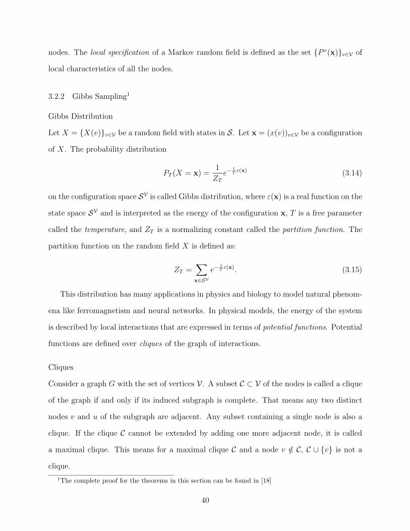
nodes. The local specification of a Markov random field is defined as the set {P v(x)}v∈V of

local characteristics of all the nodes.

3.2.2 Gibbs Sampling1

Gibbs Distribution

Let X = {X(v)}v∈V be a random field with states in S. Let x = (x(v))v∈V be a configuration

of X. The probability distribution

PT (X = x) =1

ZTe−

1Tε(x) (3.14)

on the configuration space SV is called Gibbs distribution, where ε(x) is a real function on the

state space SV and is interpreted as the energy of the configuration x, T is a free parameter

called the temperature, and ZT is a normalizing constant called the partition function. The

partition function on the random field X is defined as:

ZT =∑x∈SV

e−1Tε(x). (3.15)

This distribution has many applications in physics and biology to model natural phenom-

ena like ferromagnetism and neural networks. In physical models, the energy of the system

is described by local interactions that are expressed in terms of potential functions. Potential

functions are defined over cliques of the graph of interactions.

Cliques

Consider a graph G with the set of vertices V . A subset C ⊂ V of the nodes is called a clique

of the graph if and only if its induced subgraph is complete. That means any two distinct

nodes v and u of the subgraph are adjacent. Any subset containing a single node is also a

clique. If the clique C cannot be extended by adding one more adjacent node, it is called

a maximal clique. This means for a maximal clique C and a node v /∈ C, C ∪ {v} is not a

clique.

1The complete proof for the theorems in this section can be found in [18]

40

Gibbs Potential

A collection {VC}C⊂V of functions VC : SV → R is called a Gibbs potential on the topology

G = (V , E) with state space S if they meet the following conditions:

• if C ⊂ V is not a clique, then VC is zero.

• Let C ⊂ V be a clique. Consider two configurations x,x′ ∈ SV . If the state

of the nodes in the clique C is equal in both x and x′, then the value of the

function is identical for both inputs x and x′:

x(C) = x′(C)⇒ VC(x) = VC(x′). (3.16)

The second condition means that the value of each function depends only on the state of the

nodes inside the input clique.

If the energy function ε : SV → R can be written as

ε(x) =∑C⊂V

VC(x), (3.17)

then ε is said to be derived from the potential {VC}C⊂V .

Gibbs Fields and Markov Fields

A random field with Gibbs distribution (aka Gibbs Field) is a Markov random field relative

to a neighborhood system if the energy function of the Gibbs distribution (3.14) can be

derived from a potential relative to the same neighborhood system. Let X be a random field

with a state space S and a Gibbs distribution P . Let the energy function ε(x),x ∈ SV of

(3.14) derive from a Gibbs potential {VC}C∈V on the graph G = (V , E). It can be proved

that X is a Markov field on G, and the local characteristic of each node is given by:

P v(x) =e−

∑C3v VC(x)∑

y∈S e−

∑C3v VC(y,x(V\v))

(3.18)

where C 3 v means the cliques C that contain the node v. In the above equation, VC(y,x(V\v))

means the value of the function VC over a clique C where the state of all the nodes except v

is derived from the configuration x, and the state of v is y.

41

Note that the right-hand side of (3.18) only depends on the state of v and its neighbors.

So the condition (3.12) is satisfied. To derive the local specification (3.18), we first use the

definition of conditional probability:

Pr(X(v) = x(v)|X(V\v) = x(V\v)) =P (x)∑

y∈S P (y,x(V\v)). (3.19)

By splitting the energy function ε(x) into two groups of terms, the cliques that contain

the node v, and the ones that do not contain the node v, we will have:

P (x) =1

Ze−

∑C3v VC(x)−

∑C63v VC(x). (3.20)

For simplicity and without loss of generality, we have omitted the temperature variable T of

(3.14) in (3.20). Similarly:

P (y,x(V\v)) =1

Ze−

∑C3v VC(y,x(V\v))−

∑C63v VC(y,x(V\v)). (3.21)

If v is not in clique C, then VC(y,x(V\v)) = VC(x) independently of y. By replacing (3.20)

and (3.21) in (3.19), and factoring out e−∑C63v VC(x), (3.18) is found.

The local energy of node v is defined as the sum of the potential functions over the cliques

that contain node v:

εv(x) =∑C3v

VC(x). (3.22)

Using this definition, we can rewrite (3.18) as:

P v(x) =e−εv(x)∑

y∈S e−εv(y,x(V\v))

. (3.23)

This indicates that a random field with a Gibbs distribution in which the energy function

is derived from a potential relative to a neighborhood is a Markov random field. Hammer-

sley Clifford theorem [68] states that if P is the distribution of a Markov random field with

respect to a graph G = (V , E), and the joint probability density of the random variables of

this field is strictly positive, then we can write the function P as

P (x) =1

Ze−ε(x) (3.24)

42

Figure 3.3: A Markov chain interpretation of a random field with two variables and a binarystate space {0, 1}. Each node of this graph represents a state of the random field. Forexample, if the current state is (0,1), the first random variable is 0 and the second one is 1.By updating one variable at a time, the new state of the Markov chain is going to be one ofthe adjacent nodes of the current state. Transition probabilities are not given.

for some energy function ε(x) deriving from a Gibbs potential over the cliques of the same

graph G. Such a random field is also called a Gibbs field.

Gibbs Sampler

In this section, we show how a Gibbs field can be sampled or simulated. As mentioned

earlier, we can look at a random field on a graph G = (V , E) with a state space S, as a

random variable with values from the configuration space SV (Figure 3.3). If the random

field changes randomly with time, we can represent it by a Markov chain and formulate it

as a random process {Xt} where each random variable Xt represents the state of the field

at time t:

Xt = (Xt(v))v∈V . (3.25)

Let the distribution of the random field be of the form P (x) = 1Ze−ε(x). We now define the

transition probability of the Markov chain (3.25) in a way that this probability distribution

can be obtained as the stationary distribution π of the Markov chain. We know that if we

run the random process for a sufficiently long time, the state distribution of the Markov

43

chain gets close to π.

We start from an initial state x. To make a transition from state Xt = x to state

Xt+1 = y, we randomly choose only one node of the random field to update. Let v be this

node. The new state of the system will be (y(v),x(V\v)), in which all other nodes preserve

their previous state, and y(v) is chosen with probability P (y(v)|x(V\v)), which is obtained

using the local specifications given by (3.18). In Section 3.2.4, we demonstrate this process

using an example.

3.2.3 Simulated Annealing

In this section, we explain how sampling can be used to solve optimization problems. Let

f : D → R be a cost function over the discrete space D that we want to minimize. Using a

gradient descent algorithm, similar to continuous domains, one can start from a point in D

and try moving in a direction that gives a lower value for f , until no better neighboring point

is found. The problem with this approach is that it might get stuck in a local minimum.

The idea of simulated annealing is to allow the system to go to the states with higher values

according to some probability in order to escape local minima. As we try more points in D,

we reduce the probability of choosing higher values. Hopefully, at the end, the system will

be in the global minimum point. This is a heuristic algorithm and does not guarantee to

find the global minimum.

Simulated annealing can also be used in conjunction with Gibbs sampling. Let’s assume

we want to find the state with the minimum energy (or maximum probability). By adding

a variable T to the local specification in (3.23), we have:

P vT (x) =

e−1Tεv(x)∑

y∈S e−1Tεv(y,x(V\v))

(3.26)

where T is called the temperature variable. The name temperature is used to imply that this

process is simulating the annealing process in metallurgy, a technique involving controlled

cooling of a heated material to increase its ductility and reduce its hardness [4]. Initially, T

44

has a relatively large value. By sampling using the local specification in (3.26) and lowering

the temperature variable slowly enough (aka annealing), it has been shown that the samples

will eventually converge to the state with the minimum global energy [18].

3.2.4 Sample Usage

In this section, we summarize the Gibbs Sampler and using an example, we show how it

can be used to solve optimization problems in distributed environments, such as computer

networks. The general framework for distributedly optimizing an objective function provided

in [15] is the basis of our model. Consider a network represented by a graph G = (V , E),

where V is the set of network devices. For example, the devices in this network can be WiFi

access points, cellular base stations, IP routers, nodes in a wireless Ad Hoc network, etc.

We denote by Nv the neighbors of node v, which does not contain v. We assign an internal

state x(v) to each node v. This state, for instance, can represent the operating frequency

channel of a WiFi access point, the transmit power of a cellular BS, or the queue length of

a router. The values of these state variables are chosen from finite state spaces. Also, we

define a local objective function Fv for each node v. The value of this function for each node

depends only on the state of the node, x(v), and the state of its neighbors, x(Nv). The local

objective function can be, for example, the throughput of a base station, which depends on

the state (selected channel) of the BS and its neighboring BSs. The edge set E of the graph

is defined in a way such that v, u ∈ V are connected if and only if Fv(.) depends on x(u)

(which means Fu(.) also depends on x(v) since the graph is undirected).

We seek to optimize a global objective function F (.) over all the states x(V) in this

network. This function must be the sum of the individual local objective functions:

F (x) =∑v∈V

Fv(x).

Unlike many convex optimization methods, F does not have to be concave (in case of

maximization) or convex (in case of minimization). In the rest of this section, without loss

45

Figure 3.4: A sample network

of generality, we assume that the objective function is to be maximized.

In the previous sections, we showed that a random field with probability distribution

(3.14) is a Markov random field over a neighborhood system with the local specifications

given by (3.26) if the energy function can be written as the sum of potential functions over

that neighborhood. Now we show that there is a neighborhood system over the nodes of G

such that F can be written as the sum of potential functions Fc.

Let’s assume we want to update node b in Figure 3.4. Initially, nodes are assigned an

arbitrary state. Node b asynchronously updates its own state x(b) to a new state y(b) using

the following probability distribution:

Pr(y|x(V\b)) =e

1TF (y,x(V\b))∑

y′∈S(b) e1TF (y′,x(V\b))

(3.27)

where S(b) is the state space of node b. As we mentioned above, the global objective function

F is the sum of the local objective functions. When calculating (3.27) for node b, we can

write F as:

F (x) = Fb(x) +∑v∈Nb

Fv(x) +∑

v/∈{b}∪Nb

Fv(x) (3.28)

One can observe that after factorization, the right-hand side of (3.27) when updating node b

only depends on Fa, Fb and Fc, and is independent of Fd and Fe. The reason is that the last

term of (3.28) can be factored out from the numerator and denominator of (3.27). Thus,

node b must only be able to calculate its own objective function Fb, as well as its neighbors’

Fa and Fc. In order to calculate the latter functions, node b needs to know the state of

46

Figure 3.5: Two-tier neighborhood of Figure 3.4. Dotted edges are added to the originalgraph.

the neighbors of nodes a and c. Therefore, without any knowledge of x(e), and by knowing

the state of its two-tier neighbors x(a), x(c) and x(d), node b is able to find the probability

distribution (3.27) for the next update.

In some special cases, however, knowledge of the direct neighbors are enough, and node

b can calculate the probability distribution (3.27) without knowing x(d). For example, if

Fc(x(c), x(b), x(d)) can be written as the sum of two separate functions F 1c (x(c), x(b)) +

F 2c (x(c), x(d)), then node b does not need to calculate F 2

c , since it does not depend on b and

will be factored out in (3.27) because of the exponential nature of this probability function.

We define the two-tier neighborhood N 2v of node v as

N 2v = {u ∈ Nw|w ∈ Nv, u 6= v} (3.29)

and denote by G′ = (V , E ′) a new graph, called Gibbs sampler graph, in which the nodes are

the same as the original graph G, and two nodes are connected if they are in the two-tier

neighborhood of each other. Note that if u ∈ N 2v , then v ∈ N 2

u . Two-tier graph of Figure 3.4

is shown in Figure 3.5.

If u1 and u2 are neighbors of v in the original graph G, then u1 and u2 are adjacent edges

in G′. This means that for any node v, the set N+v = Nv ∪ {v} forms a clique on the Gibbs

sampler graph G′. Remember that Fv depends only on the state of v and its neighbors.

Therefore, we have found a neighborhood system G′, and a set of (potential) functions Fv

on cliques of G′ that add up to the global energy function F . So according to Section 3.2.2,

47

state variables xv form a Markov random field with a steady state distribution given by

(3.14) where ε(x) = −F (x) and local specification given by (3.26) where

εv(x) = −∑u∈N+

v

Fu(x(N+u )). (3.30)

Note that the utility functions are prepended by a minus sign, in order to cancel out the

minus in the Gibbs measure. The minus sign is used in the original formulation to emphasize

the minimization of the energy function. Thus, using simulated annealing described in Sec-

tion 3.2.3 and an appropriate speed for temperature reduction, the state with the maximum

probability can be found, which according to (3.14) yields the optimum value of the global

objective function.

48

Chapter 4

Methodology

In this chapter, we describe the methodology used in this work. Specifically, in Section 4.1,

we identify the contributions and specify the assumptions. Section 4.2 describes the system

model and formulates the optimization problem. The proposed distributed algorithm to

solve the optimization problem is explained in Section 4.3.

4.1 Overview

We develop an algorithm to solve an optimization problem that models the trade-off between

total throughput of the users and energy consumption of the base stations in a heterogeneous

cellular network. To this end, we find the answer to the following questions:

1. Which base stations should remain active and which ones should be powered

off in order to save energy and maintain a high throughput?

2. In each macro-BS, what proportion of a frame duration should be dedicated

to ABS subframes?

3. What is the optimal output RF power level for a macro-BS during ABS sub-

frames?

4. How many subframes should be allocated to each user during a radio frame?

The main advantage of our algorithm is that it works in a distributed fashion. That means

there is no need for a central scheduler and BSs only communicate and exchange information

in a local neighborhood, and yet the system achieves global optimality. We also consider

fairness when allocating resources to users in order to prevent starvation of some users.

49

4.2 System Model

4.2.1 General Assumptions

The following general assumptions have been made in this work. These assumptions are

commonly made in the literature as explained below.

• There is no limit to the amount of data that a user receives. That is, there is always a

packet available to be sent to each user. This is known as the infinite backlog model in

the literature.

• We only focus on downlink traffic, where data is sent from BSs to users. Orthogonal

channels are used for uplink and downlink, and there is no interference between them (as

in [19]).

• Our algorithm can be adapted for slowly varying dynamic topologies (as in [51]). We

assume the rate of users joining and leaving the network is slow compared to the time

scale on which the scheduler operates (e.g., minutes compared to milliseconds).

• The energy cost of powering a BS on or off is negligible and not considered in the model

(e.g., see [16,64]).

4.2.2 Network Topology

Consider a heterogeneous cellular network with a set of base stations B consisting of macro-

BSs B(M) and pico-BSs B(P). Each base station b ∈ B has a maximum transmit power

PMaxb , and periodically transmits a reference signal at this power. We denote by U the set

of user devices of the network. The strength of the reference signal received by user u from

base station b is given by

P(R)u,b = PMax

b Hb,u (4.1)

where Hb,u denotes the channel gain between BS b and user u, which includes all propagation

impairments such as path loss and fading.

50

Each user u receives reference signals from possibly several base stations. Theoretically,

the signal from every base station, no matter how far, can be heard by u. In practice,

however, a receiver has a sensitivity threshold and cannot detect signals that are too weak.

Thus, if the signal strength is too weak, it can be ignored by the user, since it has no

significant effect on the data rate of the receiver. This assumption is widely used in the

literature [20, 29, 57]. So the set of base stations that can serve or impact the rate of a user

u is defined as

Bu = {b ∈ B|P (R)u,b ≥ θ} (4.2)

where θ is a constant threshold known by all the nodes in the network. We assume that the

base stations are deployed in a way such that Bu is non-empty for all the users:

∀u ∈ U : ∃b ∈ B, b ∈ Bu. (4.3)

In practice, a user u is served by the base station bu that can provide the strongest signal

to u, that is,

bu = arg maxb∈Bu

P(R)u,b , (4.4)

where bu can be either a macro-BS or a pico-BS. The value of the variable bu is not fixed

during the runtime of the algorithm, and depends on the state of base stations. For example,

by shutting down a pico-BS, the users previously connected to it should now be offloaded to

their next best candidate BS.

4.2.3 Frame Structure

We consider one frequency channel that is divided into frames of a specific length. Each frame

is further divided into smaller subframes. Base station b schedules subframes of each frame,

i.e., allocates subframes to its users denoted by Ub. Subframes are not evenly distributed

among the users. In fact, the fraction of subframes that are dedicated to a user depends on

its signal to noise ratio with the goal of maximizing the throughput of the cell. Note that

scheduling is not necessarily performed for each individual frame. A base station may repeat

51

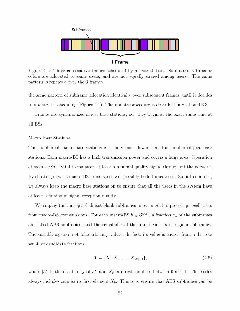
Figure 4.1: Three consecutive frames scheduled by a base station. Subframes with samecolors are allocated to same users, and are not equally shared among users. The samepattern is repeated over the 3 frames.

the same pattern of subframe allocation identically over subsequent frames, until it decides

to update its scheduling (Figure 4.1). The update procedure is described in Section 4.3.3.

Frames are synchronized across base stations, i.e., they begin at the exact same time at

all BSs.

Macro Base Stations

The number of macro base stations is usually much lower than the number of pico base

stations. Each macro-BS has a high transmission power and covers a large area. Operation

of macro-BSs is vital to maintain at least a minimal quality signal throughout the network.

By shutting down a macro-BS, some spots will possibly be left uncovered. So in this model,

we always keep the macro base stations on to ensure that all the users in the system have

at least a minimum signal reception quality.

We employ the concept of almost blank subframes in our model to protect picocell users

from macro-BS transmissions. For each macro-BS b ∈ B(M), a fraction xb of the subframes

are called ABS subframes, and the remainder of the frame consists of regular subframes.

The variable xb does not take arbitrary values. In fact, its value is chosen from a discrete

set X of candidate fractions:

X = {X0, X1, · · · , X|X |−1}, (4.5)

where |X | is the cardinality of X , and Xis are real numbers between 0 and 1. This series

always includes zero as its first element X0. This is to ensure that ABS subframes can be

52

disabled for a macro-BS if it is not required, e.g., when there is no pico-BS operating close

to the macro-BS, or when for any other reason having ABS subframes does not improve the

utility of the network. The rest of the numbers, Xis when 0 < i < |X | form an ascending

series:

∀i, j ∈ Z+|X |−1 : i < j → Xi < Xj. (4.6)

The difference between ABS and regular subframes lies in the amount of transmission

power allocated to them. In regular subframes, each macro-BS b transmits data signals to its

associated users at its maximum available power PMaxb . To comply with feICIC technology

(see Section 2.2.3), in ABS subframes, macro-BSs use a lower power level to mitigate the

interference on picocells. For a macro-BS b, this reduced power level is represented by a real

number yb that is used to scale the transmission power of the base station b as

yb · PMaxb . (4.7)

Equivalently, yb is the fraction of the maximum power that is used during ABS subframes.

Similar to xb variables, ybs are also selected from a discrete set Y = {Yi}0≤i<|Y| of candi-

date power level ratios. We have

Y = {Y0, Y1, · · · , Y|Y|−1}. (4.8)

Similarly, Yis are real numbers between 0 and 1, and zero is included as Y0 to be able

to have zero-power almost blank subframes when it is really necessary to mute all the data

transmissions from a macro-BS during ABS subframes in order to maximize the total network

throughput. The remaining numbers construct an increasing sequence of ratios:

∀i, j ∈ Z+|Y|−1 : i < j → Yi < Yj. (4.9)

The variables xb and yb are assigned per macro-BS and may differ from one BS to another.

This adds a degree of freedom to our method, compared to the approaches with a unified

fraction of ABS subframes all over the network, as in [72]. In those cases, some macro-BSs

53

Figure 4.2: A sample frame structure for a macro base station. The green area shows ABSsubframes with reduced signal power. The blue area shows the regular subframes withmaximum transmission power. In this figure, the set X of possible options for fraction ofABS subframes contains 4 elements. The BS has selected X2, while X1 and X3 are shownby dotted lines, and X0 lies on the left edge of the frame.

may waste their resources by having a large ABS ratio without the existence of any picocell

in their vicinity. On the other hand, some loaded picocells may suffer from having short

ABS durations, in order to maximize the net throughput with this restriction. In our model,

however, macro-BSs adjust their ABS duration based on the picocells in their neighborhood.

The same is true for the signal power level in ABS subframes. Each macro-BS can utilize

these subframes according to its neighboring picocells, and can vary in the range of zero

transmit power, like in eICIC, to power levels close to PMaxb .

Note that the sets X and Y are pre-defined and known to all macro base stations. Also,

ABS subframes will all be placed in the beginning of each frame by the scheduler in macro-

BSs. This makes it possible for a picocell to have some macro-transmission-free subframes

at the beginning of each frame, unless one of its neighboring macro base stations has decided

not to have ABS subframes.

Figure 4.2 depicts a frame from the point of view of a macro-BS.

Pico Base Stations

Pico base stations are less expensive and have lower transmit powers compared to macro

ones, and are situated in coverage holes or densely populated areas. For example, they

may be located near sport stadiums, shopping malls, or movie theatres. In these places,

the demand varies greatly over time, e.g., based on the events that are taking place. The

presence of a pico-BS might be unnecessary when it is only serving very few users, and it

might not be cost effective to have it running due to its power consumption.

54

Figure 4.3: Transmit power of a pico base station in operating state during a frame. Through-out the frame, the pico-BS uses the maximum available power for transmission. CandidateABS ratio for macro-BSs is the same as in Figure 4.2.

In our model, pico base stations can be in one of two states. If having them in operational

state is not advantageous, we switch them to standby (sleep) mode. In standby mode, a pico-

BS is almost shutdown, except for a small processor and accessories that allow it to contact

other base stations and see whether it should wake up or not. So it neither broadcasts a

reference signal nor serves users in standby mode, and users are not aware of its existence.

That means the transmission power of a pico-BS in this state is zero and it has no interference

on the users.

If, on the other hand, the density of users close to a pico-BS is high, it is powered on.

In this mode, in contrast with macro base stations, a pico-BS b always transmits at its

maximum power level PMaxb and does not have ABS subframes. We denote by a binary

variable zb the state of a pico-BS b:

zb∈B(P) =

1 b is fully functional

0 b is in standby mode

(4.10)

Figure 4.3 illustrates the transmit power of a picocell during a frame.

Interference on Users

The amount of interference on a user depends on the status of its neighboring base sta-

tions and varies even during one frame. For instance, a user of a macrocell suffers from

less interference when a neighboring pico-BS is powered off. Moreover, because different

macro-BSs may have different fractions and powers for ABS subframes, the amount of in-

terference changes within a single frame. To better understand this, consider the network

in Figure 4.4. User U1 is served by the base station A and interfered by B, C and D. The

55

Figure 4.4: Multiple macro-BSs interfering with a user. U1 is served by base station A. OtherBSs have different number of ABS subframes. During the subframes in green rectangles,macro-BSs are in ABS mode. During the rest of the frame (Blue area), macro-BSs transmitat their maximum power. Figure 4.5 shows the interference on U1 over one frame.

number of ABS subframes varies among the interfering base stations. For example, in the

subframes between X0 and X1, all the interfering macrocells are in ABS mode, while during

the subframes between X2 and X3, only base station D is in ABS mode, and the other two

neighboring macro base stations are transmitting at their maximum power. Consequently,

the interference on U1 differs from one subframe to another.

We denote by Ti the sequence of subframes between two consecutive candidate ABS

fractions Xi and Xi+1 where 0 ≤ i < |X |. According to Figure 4.4 and the above explanation,

the interference on a user does not change within the subframes of Ti, however, it is likely

56

Figure 4.5: Interference on a user during a frame. The more pale the color is, the lessinterference the user suffers. During the last period, all the macro-BSs are at their maximumpower.

to change from Ti to Ti+1.

A user may experience a maximum of |X | different interference levels (see Figure 4.5).

Note that the actual number of distinct interference powers may be less than this number.

First of all, the number of macro-BSs in Bu may be less than |X | for a user u. Also, more

than one macro-BS may choose the same ABS fraction. For example, if all macro-BSs in

Bu select the same fraction Xi, user u will only experience two different interference levels.

Furthermore, if this Xi equals zero, then the interference on u will be constant over the

entire frame, since all the macro-BSs are transmitting at their maximum power during every

subframe of a frame.

To formulate the total interference on user u, we first define P ib as the transmit power

level of BS b during period Ti. One can simply observe that for a pico-BS, this value only

depends on whether it is on or off:

P ib∈B(P) =

PMaxb zb = 1

0 zb = 0

(4.11)

For a macro-BS, P ib depends on the ratio of ABS subframes xb and transmit power of the

BS during ABS and regular subframes:

P ib∈B(M) =

PMaxb xb ≤ Xi

yb · PMaxb xb > Xi

(4.12)

Using the above notations, we can calculate the total interference on user u during each

57

period Ti:

Intiu =∑b 6=bu

P ibHb,u (4.13)

Note that as shown in Figure 4.5, the amount of interference increases from the beginning

of the frame toward the end:

Int0u ≤ Int1u ≤ Int2u ≤ · · · . (4.14)

This happens because as time passes within a frame, more neighboring macro-BSs make

transition from ABS subframes to regular subframes.

4.2.4 User Rates

Because of the difference in both interference and signal power, the signal to interference

and noise ratio (SINR) of each user u varies in different periods Ti of a frame. It can be

formulated as

SINRiu =

P ibu

Intiu +N0

. (4.15)

As a result, base stations schedule each period separately. Each user gets a portion of

subframes of each period. To maximize the utility function, a user may get more shares in

Ti and less shares in Tj. For example, imagine that base station A has no ABS subframes

in Figure 4.4. In this case, all the subframes are equally valuable to U2, i.e., they can carry

the same amount of data, since there is no interference on this user. On the other hand, a

subframe in T1 is more beneficial to U1 than a subframe in T2, since SINR1U1

is higher than

SINR2U1

. Therefore, BS-A can allocate the beginning subframes of each frame to U1, and

U2 gets more subframes toward the end of the frame, in order to best utilize the channel.

We denote by wiu the fraction of subframes of a frame that BS b allocates to user u ∈ Ub

during Ti:

∀b ∈ B, 0 ≤ i < |X | :∑u∈Ub

wiu = Xi+1 −Xi. (4.16)

58

The right-hand side of the above equation is the ratio of duration of Ti to the frame length

(see Figure 4.5). The following equation is derived from the definition of wiu variables:

∀b ∈ B,|X |−1∑i=0

∑u∈Ub

wiu = 1. (4.17)

To map an SINR to a rate, we use the Shannon capacity formula:

ciu = B log2(1 + SINRiu) (4.18)

where ciu is the total rate that can be achieved by the user u during Ti if all subframes in Ti

are allocated to u. The parameter B is the bandwidth of the channel. Thus, the rate of user

u during the time period Ti can be obtained by the following formula:

riu = wiuciu (4.19)

Finally, the average bit rate of user u during a frame can be written as the sum of the

rates over all the periods:

Ru =

|X |−1∑i=0

riu. (4.20)

4.2.5 BS Power Consumption

For the energy consumption of base stations, we follow the model proposed in [46] and

adopted by [16] and [64]. According to this model, the energy consumption of a BS is given

by:

W =

NTX(P0 + ∆P · PTX), PTX > 0

NTX · Pidle, PTX = 0

(4.21)

where NTX is the number of antennas, P0 is the power consumption at zero RF output

power, PTX is the RF output power, Pidle is the power consumption of the base station in

standby mode, and ∆P is the slope of the load-dependent power consumption.

For simplicity, we assume the number of antennas NTX equals 1. Note that P0, Pidle and

∆P are predefined parameters. For a pico-BS b, RF output power is either zero or PMaxb . So

59

we have

Wb∈B(P) =

P0 + ∆P · PMax

b , zb = 1

Pidle, zb = 0

(4.22)

Macro-BSs have different RF powers during a frame. Thus, we calculate the average RF

power in a frame in order to find the energy consumption of a macro-BS:

PTX = xb · (yb · PMaxb ) + (1− xb) · PMax

b . (4.23)

By replacing (4.23) in (4.21), we have:

Wb∈B(M) = P0 + ∆P · PMaxb

(xb · yb + 1− xb

). (4.24)

4.2.6 Optimization Objective

We define a utility function U(.) over user rates, and a cost function C(.) over power con-

sumption of base stations. Any continuously differentiable concave function is suitable as the

utility function. The simplest choice would be the summation of user throughputs. However,

this function usually leads to a case in which each base station dedicates all its resources

to one or a few users (the ones with highest channel gain), and leaves other users starving.

Another option would be to adopt a logarithmic utility function to achieve proportional

fairness:

U(R) =∑u∈U

log(Ru), (4.25)

where R is the vector of bit rates of all users. In our simulations in Chapter 5, we evaluate

both logarithmic sum and linear sum utility functions, which are concave and continuously

differentiable.

For the power cost function, we simply add up the energy consumed by all the base sta-

tions:

C(W) =∑b∈B

Wb, (4.26)

where W denotes the vector of BS energy consumptions.

60

Finally, we denote by λ a weight factor between total throughput and total energy con-

sumption, and write the optimization objective as

F (R,W) = U(R)− λ · C(W) (4.27)

which is to be maximized. In general, throughput and energy consumption are directly

proportional. A larger value of λ increases the negative impact of energy consumption on the

objective function, and favors low-throughput and low-energy states over high-throughput

and high-energy states.

We summarize the optimization objective and the constraints in (4.28), and the set of

notations used in this model in Table 4.1.

maxx,y,z,w

F (R,W)

s.t. xb ∈ X , ∀b ∈ B(M)

yb ∈ Y , ∀b ∈ B(M)

zb ∈ {0, 1}, ∀b ∈ B(P)∑u∈Ub

wiu = Xi+1 −Xi, ∀b ∈ B

wiu ∈ [0, 1], ∀u ∈ U , 0 ≤ i < |X |

(4.28)

61

Table 4.1: Notations used in the model.

Notation Description

U Set of usersUb Set of the users that are associated to BS bB Set of base stations

B(M) Set of macro base stations

B(P) Set of pico base stationsBu Set of base stations that can serve user ubu The base station that serves user u

PMaxb Maximum RF output power of BS bP ib RF output power of BS b during Ti

P(R)u,b Received power of the reference signal of base station b at user u

yb Fraction of max RF output power that a macro-BS uses in ABS modeY Set of possible values for ybYi ith element of Yzb Binary variable indicating whether a pico-BS is in sleep modeθ Minimum received power threshold from a BS to a user in its rangexb Fraction of a frame length in which BS b is in ABS modeX Set of possible values for xbXi ith element of XTi Fraction of a frame from Xi to Xi+1

Intiu Total interference on user u during period Ti of a frameSINRi

u SINR of user u during period Ti of a frameciu Spectral efficiency of user u during period Ti of a frameHb,u Pathloss (or channel gain) between BS b and user uN0 Noise powerB Bandwidth of a frequency channelwiu Fraction of subframes of a frame that BS bu allocates to user u during Tiriu Bitrate of user u during period Ti of a frameRu Average bitrate of user u during one frameWb Average energy consumption of a base station during a frameNTX Number of antennas on a BSPidle Energy consumption of a base station in standby modeP0 Energy consumption of a running BS at zero RF output power∆P Slope of the load-dependent energy consumption of a BSPTX RF output power of a BSU(.) Utility function over user ratesC(.) Cost function over energy consumption of base stationsF (., .) Objective functionλ Weighting factor to balance bitrate and energy consumption

62

4.3 Solution

4.3.1 Overview

The optimization problem in (4.28) contains a mixture of real variables w, discrete variables

x and y, and binary variables z. Here we use an optimization technique known as meta-

optimization, in which one optimization problem is solved and the results are fed into another

one. In our case, each base station locally solves a convex optimization problem, and uses

its solution in a larger-scale distributed algorithm in order to optimize the global objective

function as defined in (4.27).

We begin by breaking the global utility and cost functions for the network into the sum

of local utility and cost functions for each BS. According to (4.26), the local cost function

can be easily written for each BS. Let Cb denote the cost of base station b. We have:

Cb = Wb. (4.29)

The global utility function (4.25) is defined over user rates. We know that each user

is associated to one base station, which is the one with the strongest received signal1. So

if we write the local utility function for each base station as a function of the rates of the

users associated to it, we obtain the global utility function as the sum of local ones over the

base stations. Let Ub denote the local utility of base station b. We have:

Ub =∑u∈Ub

log(Ru). (4.30)

Therefore, the local objective function can be written as:

Fb = Ub − λ.Cb, (4.31)

where Fb denotes the local objective function at base station b. Now the global objective

1Theoretically, a user may not be associated to any BS, for example when all the BSs in range are picoand they are all in sleep mode. This is very unlikely to happen because of the logarithmic utility functionthat returns −∞ if the rate of a user is zero. Even in that case, equation (4.30) still holds.

63

function can be written as the sum of local ones:

F (R,W) =∑b∈B

Fb. (4.32)

Evidently, to maximize the global objective function (4.27), we cannot simply maximize

each local function of form (4.31) independently of the others. Maximizing an individual

local objective would negatively impact other base stations. To see this, let’s take a closer

look at the optimization variables of (4.28). It is obvious that if a BS b modifies any of xb, yb

or zb (in case of a pico-BS), it affects the performance of some other cells. Turning a pico-BS

on or off may lead to changes in user associations, and also in the amount of interference

on users of other cells. Similarly, changing the duration and power of ABS subframes of

a macro-BS changes the interference level of users of other cells during different parts of a

frame.

On the other hand, internal scheduling of each base station, i.e., the amount of resources

that the BS allocates to each user, does not affect other cells. No matter how a BS allocates

subframes to its users, the amount of interference it imposes on the users of other cells

remains the same. In fact, BS b adjusts the values of wius in order to optimize its own utility

function, without having any influence on other cells. This is due to the fact that the RF

output power of a BS during a frame is specified by variables xb and yb. Therefore, in our

meta-optimization, we optimize wius individually for each BS in a local manner since they

only change the local utility function. The optimal values of xbs, ybs and zbs are found

distributedly by exchanging information in a local neighborhood, since these variables also

change local objective functions of other cells.

With the above explanation in mind, the next section describes how we incorporate Gibbs

Sampling described in Chapter 3 to solve the problem in a decentralized way.

64

Figure 4.6: Interaction graph.A is connected to B and C, because they have common users in their range.A is not connected to D and E, because they have no common user in their range.

4.3.2 Gibbs Sampler

In this section, we define a neighborhood system, state spaces for the nodes and local energies

in order to solve the problem using the framework in Section 3.2.4. Consider a graph G that

represents the system. Nodes of this graph are the set of base stations B, both macro-BSs

and pico-BSs. In this graph, two base stations are adjacent if they have at least one common

user in their range. That is, there is an edge between b1 and b2 if:

∃u ∈ U : b1, b2 ∈ Bu (4.33)

Figure 4.6 illustrates an example neighborhood system and its corresponding graph G. We

call this graph the Interference Graph, since connected base stations in this graph directly

interfere with each other’s users. The neighbors of a node b are denoted by Nb.

Now we define a state sb for each node b. Macro-BSs and pico-BSs have different state

spaces. For macro-BSs, the states are ordered pairs of the form (xb, yb), whereas for pico-BSs

65

the state only contains the on/off state (zb). The state spaces are defined as:

Sb =

X × Y b ∈ B(M)

{0, 1} b ∈ B(P)(4.34)

Note that the size of the state space of a macro-BS is not |X | × |Y|. The reason is that

the first element of X is zero, and if there is no ABS subframe (xb = 0), the macro-BS b

behaves the same no matter what the value of yb is. So the size of state space of macro-BSs

is 1 + |Y|(|X | − 1).

To calculate the local objective function Fb, each base station only needs to know its own

state, and the state of its neighbors. That is, each BS should be informed of whether its

pico neighbors are on or off, and what is the power and time duration of ABS subframes in

its macro neighbors. Using this information, the only missing variables to calculate the local

objective function of base station b in (4.31) are the shares wiu, u ∈ Ub of each user associated

to b. Indeed, we can verify that by knowing zb′ , xb′ and yb′ for all the base stations b′ ∈ Nb

plus b itself, each BS b is able to:

• Determine the BS that each user in the range of b is associated with.

• Calculate the signal to interference and noise ratio (4.15) for each user in its

range during different periods of a frame.

• Calculate the energy consumption of each neighboring BS using (4.22) and

(4.24).

Then to find user shares, each base station b should solve the following optimization

problem:

arg maxwi

u

Fb (4.35)

given the values of z, x, and y for b and its neighbors, and the last two constraints in the

66

main optimization problem (4.28) which are repeated here for convenience:∑u∈Ub

wiu = Xi+1 −Xi, ∀b ∈ B

wiu ∈ [0, 1], ∀u ∈ U , 0 ≤ i < |X |

Note that the problem in (4.35) is a convex optimization problem. To understand this,

recall that the values of SINR (4.15), and therefore spectral efficiency (4.18) and energy

consumption (4.22) and (4.24) become constants given the states of the nodes in the neigh-

borhood of b. Thus the local utility function becomes the sum of concave (logarithmic or

linear) functions over a linear combination of optimization variables wiu. The constraints are

also linear. Thus, problem (4.35) is an ordinary convex optimization problem that can be

solved using the standard methods in the field of convex optimization. In Section 3.1, we

briefly touched upon convex optimization techniques. Here, we leave out the full steps of

solving (4.35) and concentrate on our main contribution, which is solving the global opti-

mization problem using Gibbs Sampling.

To this end, the value of the local objective function of each node b in graph G is the

value of Fb using the following inputs:

• states z, x, and y of b and its neighbors Nb,

• the optimal solution of (4.35).

To find the local energy, as mentioned in Section 3.2.4, each node b needs to calculate

its own local objective function and those of its neighbors Nb. To find the latter, a node

needs to have the states of its two-tier neighbors. We construct the graph G′, which we call

the two-tier neighborhood graph, according to Section 3.2.4. Then each node b obtains the

states of its neighbors in G′ denoted by N 2b . The local energy of each state sb ∈ Sb based on

(3.30) is defined as:

εb(sb) =∑b′∈N+

b

Fb′ , (4.36)

67

where N+b is the set of b and its neighbors:

N+b = Nb ∪ {b}. (4.37)

To find the right-hand side of (4.36), the state of node b is given as an input of the function

εb(.), states of two-tier neighbors are fixed and obtained through communication among

neighbors as described in the next section, and shares of users are found by solving the

optimization problems of the form (4.35).

Finally, the transition probability of node b is of the form (3.26), which is defined as:

Pr(s ∈ Sb|sN 2b) =

e1Tεb(s)∑

s′∈Sb e1Tεb(s′)

(4.38)

where sN 2b

denotes the states of the base stations in N 2b .

4.3.3 Distributed Algorithm

We break the protocol into two phases. The first phase, initialization, is intended so that

the base stations become familiar with their neighborhood, i.e., the users and other BSs

that they are directly affecting. This is required in order for them to internally build their

perception of the interference graph, and also to be able to calculate user rates.

Using the information received in the first phase, BSs then start the iterative phase.

By repeatedly updating its internal parameters according to the specified rules, the system

converges to the optimal state that maximizes the global objective function given in (4.27).

Initialization Phase

Initially, all the picocells are on. Users connect to the BS with the highest reference signal

received power. Each BS b requests each of its users u to report the list of all BSs they can

hear (denoted by Bu), and their channel gains (denoted by Hb,u). Using this information, in

Figure 4.6 for example, BS A will add BS B to the list of its neighbors. BS A is still not

aware of BS C, because their mutually interfered user is connected to C. Likewise, BS B is

still unaware of BS A.

68

Then each BS sends the information gathered from its users to each of the neighboring

BSs that it has identified so far. This way, BS A will recognize BS C as its neighbor, by

receiving the list of users of C. Now every BS can make a complete list of its first tier

neighbors Nb.

Next, they exchange their maximum RF output power PMaxb , their initial state, and their

neighbor list with their immediate neighbors Nb. By processing these received lists, BSs can

construct their two-tier neighbor list N 2b . The system assumes a default initial state for

every base station, e.g., all pico-BSs are active and all macro-BSs are in full power mode.

Iterative Update Process

Once the previous phase is completed, all the BSs start the next phase at the same time.

From this point on, the iterative update process does not have to be supervised by a scheduler,

and each BS is updated independently of the others. For example, the base stations do not

have to be updated sequentially in the same order in each iteration. A BS may update its

state multiple times before another BS is updated once.

At the start of this phase, each BS b randomly chooses a timeout between 0 and τ , and

triggers an update when the timeout has expired. In an update process, a BS b selects a new

state sb from its state space, independent of its current state. To select the new state, BS

b calculates the local objective function Fb′ of every BS b′ ∈ N+b (b and its neighbors) given

each s ∈ Sb, and by adding these |N+b | objectives together, computes the local energy εb(s)

of each potential next state s 2. Then it chooses its new state according to the probability

distribution in (4.38), which is repeated here for convenience:

Pr(sb = s) =e

1Tεb(s)∑

s′∈Sb e1Tεb(s′)

. (4.39)

Here, the temperature T is a decreasing function of the time t elapsed from the beginning

of the iterative phase. This function is globally known among all BSs, and since they all

2Instead of calculating the local objective of each neighbor b′, BS b can ask its neighbors to provide theirlocal objective given the current state of b. This way there is no need for two-tier neighborhood, and eachBS only needs the information of its one-tier neighbors to compute its own local objective.

69

started the algorithm simultaneously, the temperature value remains synchronized across

all the base stations of the network. The purpose of this temperature variable is to allow

base stations to select low energy states during early stages of the iterative phase in order

to avoid getting stuck in a local optimum. As time passes, the high-energy states will be

chosen with a higher probability. An example of the temperature function is the following

( [51]):

T (t) =T0

log(2 + t). (4.40)

In Chapter 5, we evaluate this function as well as other temperature functions.

Once the BS b has selected and transitioned to its new state sb, it randomly picks another

timeout in a similar fashion to perform the next update.

If the state of b has changed in this update, it informs its two-tier neighbors. Another

option would be to inform its immediate neighbors and let them forward it to their other

immediate neighbors; however, that would cause the two-tier neighbors to receive duplicate

information from multiple neighbors.

If a pico-BS has decided to shut down as a result of an update, its users will choose their

next-best BS (if there is any). Users are constantly monitoring all the reference signals, so

once a stronger signal is heard (a pico is back on), they switch to it.

By repeating this process until convergence, the system reaches the optimal state where

each BS selects the same state at each update. At this point, the temperature is very close

to zero.

We can start the whole algorithm (from the initialization phase) over again at specific

intervals to cope with dynamic changes in the topology. During each execution, we assume

that the topology (e.g., the neighborhood system) does not change.

Speed of convergence of the system depends on the choice of the temperature function.

If we quickly decrease the temperature to zero, the convergence would be faster, at the cost

of losing optimality. Slower annealing process causes the network to take longer to converge,

70

but the energy of the converged state would be closer to that of the optimal state. In our

simulations, we observed that a few hundred iterations is enough to converge a network of

hundreds of BSs spread over a large geographical area to a near-optimal state.

71

Chapter 5

Simulation Results

In this chapter, we present a numerical study to demonstrate the effectiveness of our method

by simulating it in different scenarios. We begin with describing the simulation environment

in Section 5.1. This section also goes over some of the practical limitations of the simulation.

Next, we analyze the effect of each parameter on the accuracy and performance of the

algorithm. In Section 5.2, we run the algorithm on a HetNet and report the states of the

base stations after the convergence, e.g., which pico-BSs are in sleep mode. We also report

the throughput, energy consumption and objective of each cell, as well as the entire network.

Section 5.3 analyzes the trade-off between throughput and energy consumption. Essentially,

this section reports the statistics of the network with different values of λ in the equation

(4.27). Section 5.4 illustrates how fairly the users are served depending on the rate utility

function U(R). Section 5.5 reports the objective improvement achieved by enabling each of

the following features: zero-power ABS subframes, low-power ABS subframes, and picocell

deactivation. In Section 5.6, we investigate the outcome of our algorithm in a network

consisting of only picocells, as in [56] and [60]. Finally, Section 5.7 numerically studies the

convergence of the algorithm. In this section, we analyze 4 different factors that affect the

convergence: the temperature function, the initial temperature, duration of the process, and

the cell update rates.

5.1 Simulation Environment

We simulated the proposed algorithm in MATLAB. Two network configurations are studied

in this chapter. Throughout Section 5.2 to Section 5.5, we use a heterogeneous network

to investigate the states of both macrocells and picocells. Since macro-BSs have a large

72

state space of the size |X × Y| and all of the base stations are simulated on one machine

(contrary to the reality where each BS has its own processor), we limit the number of cells

to 19. It should be noted that this network size is adequate for prototyping purposes, and

much smaller networks have been studied in the literature, for example in [56]. For the last

two sections of this chapter, deployment of macrocells is not required. This allows us to

simulate a larger network with 400 cells, since in our model picocells have only 2 operating

states (active or sleep) as opposed to macrocells. The larger size makes the network more

suitable to graphically illustrate the convergence of our algorithm, which is provided in the

last section of this chapter.

For sections 5.2 to 5.5, we consider the cellular network in Figure 5.1, which is composed of

7 macro-BSs located in a hexagonal form. The network also consists of 12 pico base stations

located on cell edges. As in LTE networks, the frequency reuse factor is 1, i.e., all the BSs

and users operate on the same frequency. One hundred users are spread over the network

using a Poisson Point Process (PPP is a common choice for modeling users [21]). We make

sure that all the users are in the covered area and receive a signal above the threshold θ from

at least one macro or pico base station.

The large network of picocells is described in Section 5.6.

5.1.1 Simulation Parameters

Some of the parameters in Table 4.1 are algorithm-independent constants and not tunable.

For these constants, we have used the fixed values in Table 5.1 throughout all simulations.

To estimate the channel gains, we used the following path loss model:

Pr = Ptd−γ

where Pt and Pr indicate the signal power at the transmitter and receiver respectively, d is

the distance between the two, and γ is the path loss exponent with values in the range of 2

in free space to 4.5 in relatively lossy environments (see [2,67]). The parameters in Table 5.1

73

×104

0 0.5 1 1.5 2 2.5 3

×104

0

0.5

1

1.5

2

2.5

3

Figure 5.1: The simulated HetNet scenario.

are similar to the ones in [64] and mostly aligned with HetNet specific parameters considered

in [8].

Other parameters can be analyzed and by tweaking them we can change the complexity

and behavior of the algorithm and enhance the results. By default, they are defined as

follows:

• Rate utility function: We simply add the throughputs of users of a cell:

Ub =∑u∈Ub

Ru

• Objective function: As mentioned in Section 5.1.2, we use a scaling factor:

Fb = 10−4(Ub − λ · Cb)

74

Table 5.1: Simulation parameters

Parameter ValuePico-BS Macro-BS

N0 (dBm) −120θ (dBm) −90B (Hz) 5× 103

PMax (W) 0.5 20Pidle (W) 4.3 75P0 (W) 6.8 130

∆P 4 4.7γ 3.5

In this function, 10−4 is the scaling factor and λ = 200 is chosen to balance

the throughput and energy consumption.

• Initial temperature: T0 = 5

• Temperature function: We use a quadratic function with zero temperature

at tend = 103:

T (t) = T0 × (1 +t− 1

1− tend)2

• Set of possible ABS duration ratios: We consider 4 different options for

the ratio of ABS subframes:

X = {0, 1/10, 2/10, 3/10}

For instance, if a macro-BS chooses 1/10, it dedicates one tenth of subframes

of a frame to ABS mode.

• Set of possible ABS power ratios: The following 4 ratios are allowed for

ABS power ratios:

Y = {0, 1/4, 1/2, 3/4}

As an example, if a macro-BS has selected 1/2, it transmits at half of its

maximum output power during ABS subframes.

75

• Update probability: After each update, a base station refrains from updat-

ing itself for a number of iterations. This number is chosen randomly each

time from [0, τ ], where τ = 10.

Unless otherwise stated, the above parameters are used in the rest of the simulations in

this chapter. In each section, we may modify a few of these parameters to evaluate how they

influence the network.

Note that for convenience, we have limited the size of X and Y to a small number.

Although the proposed algorithm can handle large state spaces, it makes the simulations

slow, especially when a large number of base stations are simulated on one computer.

5.1.2 Implementation Remarks

During the runtime of the algorithm, each node is updated several times. In each update,

a node should calculate its own local objective function given the current state of the local

neighborhood, and all of its own possible states from the state space. Moreover, it should

calculate the local objective function of its neighbors given their current neighborhood. Each

of these local objective functions requires a convex optimization problem of the form (4.35)

to be solved. In order to speed up the process and reduce the communication overhead,

each base station maintains a cache of the functions that it has calculated so far. So for

each state, a node tries to look up the values of the local objective functions in its cache,

and only solves the convex optimization problem if the value is not in the cache yet. In the

simulations, some functions had to be evaluated with the same input for thousands of times,

and it would have been infeasible to run the simulation for a long period without caching the

convex optimization results. This feature can vastly reduce the complexity of the protocol

in real implementations.

Another practical concern is the range of the local objective functions. Remember that

the probability distribution of each state transition is given by the Gibbs distribution, which

76

has exponential terms. In MATLAB, real numbers that cannot be represented by 1024 bits

are regarded as∞, and the maximum real number in MATLAB is 1.7977×10308. That means,

without considering the temperature variable in (4.38), the practical upper bound for the

value of local energies (sum of the local objective functions) should be ln(1.7977× 10308) ≈

707. Likewise, the lower bound of these energies is approximately −707.

This limitation is not problematic in our simulations. During the simulated annealing

procedure, when the temperature gets close enough to zero, the local energy of a node in

its best state goes to +∞. This is inevitable and necessary to converge the process to the

optimal solution. For each base station, at some point when the temperature is cool enough,

the value of local energy of one of the states reaches the upper bound of real numbers in

MATLAB. From this point on, we cannot calculate the transition probabilities, which require

exponential function computations. We assume that when the local energy of a state reaches

this limit, the base station is already converged to its optimal state and no longer needs to

be updated.

For the above assumption to be correct, we need to ensure that those near-infinity values

only happen in near-zero temperatures. Therefore we have to scale the function in a way that

for the initial temperature, the local objective value is small enough so that following Gibbs

distribution is feasible for a reasonable number of iterations. This can be easily achieved

using a linear transformation of the local objective function. For example, by multiplying

the function by a positive scalar, we can obtain the desired range of outputs. Considering

the fact that the Gibbs Sampler converges to the optimal state with the highest energy, this

scaling does not corrupt the algorithm since the same state has the maximum global energy

before and after the scaling.

77

×104

0 0.5 1 1.5 2 2.5 3

×104

0.5

1

1.5

2

2.5

(a) 1-tier neighborhood

×104

0 0.5 1 1.5 2 2.5 3

×104

0.5

1

1.5

2

2.5

(b) 2-tier neighborhood

Figure 5.2: The neighborhood graph associated with Figure 5.1.

Table 5.2: Global performance measures

Final valueTotal Throughput 866705Total energy consumption 1519.7Energy saving 153.9Global objective 56.3

5.2 States of BSs After Convergence

Figure 5.3 illustrates the state of the network after the convergence of the algorithm. For

the sake of reporting, we number the cells as follows. The macrocell in the area i of the

Figure 5.3 is referred to as Mi. The picocell that is encompassed by Mi is called Pi. Also,

the picocell that overlaps Mi and Mj is referred to as Pij.

Table 5.2 reports the final values of the performance measures after the convergence of

the system. Table 5.3 shows the breakdown of measures and state of macro-BSs. Table 5.4

reports the statistics of the pico-BSs, except for the ones that are in sleep mode after conver-

gence. Those standby pico-BSs by definition consume Pidle = 4.3W energy (see Table 5.1)

and have zero throughput.

78

×104

0 0.5 1 1.5 2 2.5 3

×104

0

0.5

1

1.5

2

2.5

3

12

3

4 5

6

7

Figure 5.3: The network after convergence. Lines indicate associations. Dotted picocells arein sleep mode.

Discussion

The energy saving in Table 5.2 comes from both macro-BSs and pico-BSs. According to

(4.24) and Table 5.1, the maximum energy consumption of a macro-BS in our model is 224

watts. Because of the low-power (or zero-power) output of macro-BSs during ABS subframes,

all of them are consuming less energy. All macro-BSs have chosen to have ABS duration

ratio of 0.3 (the largest value allowed). Macro-BS M7 is consuming less energy compared to

the other ones, because it remains fully silent during the ABS subframes, while others have

decided to transmit at quarter or half the maximum power. The reason could be the fact

that M7, as shown in the neighborhood system depicted in Figure 5.2, is interfering with

more picocell users compared to other macro-BSs.

79

Table 5.3: Statistics of macro-BSs

M1 M2 M3 M4 M5 M6 M7ABS time % 30 30 30 30 30 30 30ABS power % 25 25 50 50 50 50 0Throughput 96378.4 82924.3 139554.5 101033.4 95329.3 117013.3 52921.9Energy 202.9 202.9 209.9 209.9 209.9 209.9 195.8Objective 5.6 4.2 9.8 5.9 5.3 7.5 1.4

Table 5.4: Statistics of pico-BSs

P16 P45 P34 P23 P12 P2Throughput 24273.8 79093.2 25484.6 31992.1 13669.4 7036.9Energy 8.8 8.8 8.8 8.8 8.8 8.8Objective 2.3 7.7 2.4 3 1.2 0.5

Six of the pico-BSs are in standby mode. P1, P4 and P56 have no user in their coverage,

and there is no reason for them to stay on. P3, P5 and P6 are in sleep mode because the

users in their range can get a much better throughput from macro-BSs. Other pico-BSs are

operating because the users they are serving are either not covered by macro-BSs, or are

very close to macrocell edges.

5.3 Energy-Throughput Trade-off

There is a trade-off between throughput and energy consumption in our objective function.

This means that there are many pareto optimal solutions that are theoretically considered

equally good without a subjective preference. The trade-off between the two can be adjusted

based on different viewpoints and targets. In this section, we investigate the effect of altering

the weights of the two components of the objective function. We simulate the same network

(in Figure 5.1) with the same set of parameters. Consider the objective function in (4.27),

which is repeated here for convenience:

F (R,W) = U(R)− λ.C(W).

Table 5.5 reports the converged state of the system using different trade-off weights.

80

Energy (W)

1400 1450 1500 1550 1600 1650

Thro

ughput (b

ps)

×10 5

5

6

7

8

9 0 100 2001000

2000

5000

10000

100000

Feasible region

Infeasible region

Figure 5.4: Throughput vs. energy: Pareto frontier with different optimal solutions. Thenetwork throughput is directly proportional to the consumed energy. The maximum through-put is achieved when the energy cost is zero (λ = 0) and the lowest throughput occurs atthe highest energy cost (λ = 100000).

Figure 5.4 plots the pareto frontier corresponding to those weights.

Discussion

Table 5.5 shows the decrease in both throughput and energy as we increase the energy cost.

When we are not concerned about energy, most of the pico-BSs are on. As the cost of energy

rises, fewer pico-BSs remain operating. When λ = 104, only one pico-BS (P45) remains on,

in order to serve the two users that would have been abandoned otherwise. At λ = 105, even

that pico-BS goes to standby mode and leaves the two users unserved. Also, macro-BSs

transmit at the lowest possible power when the cost of energy is extremely high, since the

utility gain is not worth the required energy.

81

Table 5.5: Effect of the energy cost on the converged state. By increasing the weight ofenergy, throughput and energy consumption are both dropped. The last column shows thenumber of pico-BSs that are on.

λ Throughput Energy Objective Avg. xi % Avg. yi % No. Pico0 874106.3 1636.4 87.4 4.3 0 10100 870214.8 1547.9 71.5 30 50 6200 866705 1519.7 56.3 30 35.7 6500 860705 1491.5 11.5 30 21.4 61000 860705 1491.5 -63.1 30 21.4 62000 849488.6 1484.4 -211.9 30 17.9 65000 729571.6 1451.7 -652.9 30 3.6 510000 582978.2 1426.7 -1368.4 30 0 1

100000 503885 1422.2 -14171.6 30 0 0

5.4 Rate Utility Function

In this section, we study the choice of rate utility function and its effect on user throughputs.

Note that this function must be of a specific form: Local rate utility functions must add up

to the global rate utility function. This means that, for example, maximizing the minimum

rate over the global network is not possible using this method, because the global minimum

rate is not equal to the sum of the local minimum rates.

We consider two options:

1. Sum rate: U(R) = 10−4∑

u∈U Ru

2. Proportional fairness: U(R) = 10∑

u∈U log(β+Ru) where β is a positive con-

stant that plays two roles: First, it prevents an undefined logarithmic function

when Ru is zero. Secondly, it controls the fairness level. The logarithmic

function achieves fairness by punishing the utility if there are users with low

bit rates. A large β makes the function less sensitive to small Ru values and

reduces the fairness.

Note that 10 and 10−4 are placed in utility functions to scale the objective function up and

down, respectively (refer to Section 5.1.2). Since we only want to investigate the fairness

82

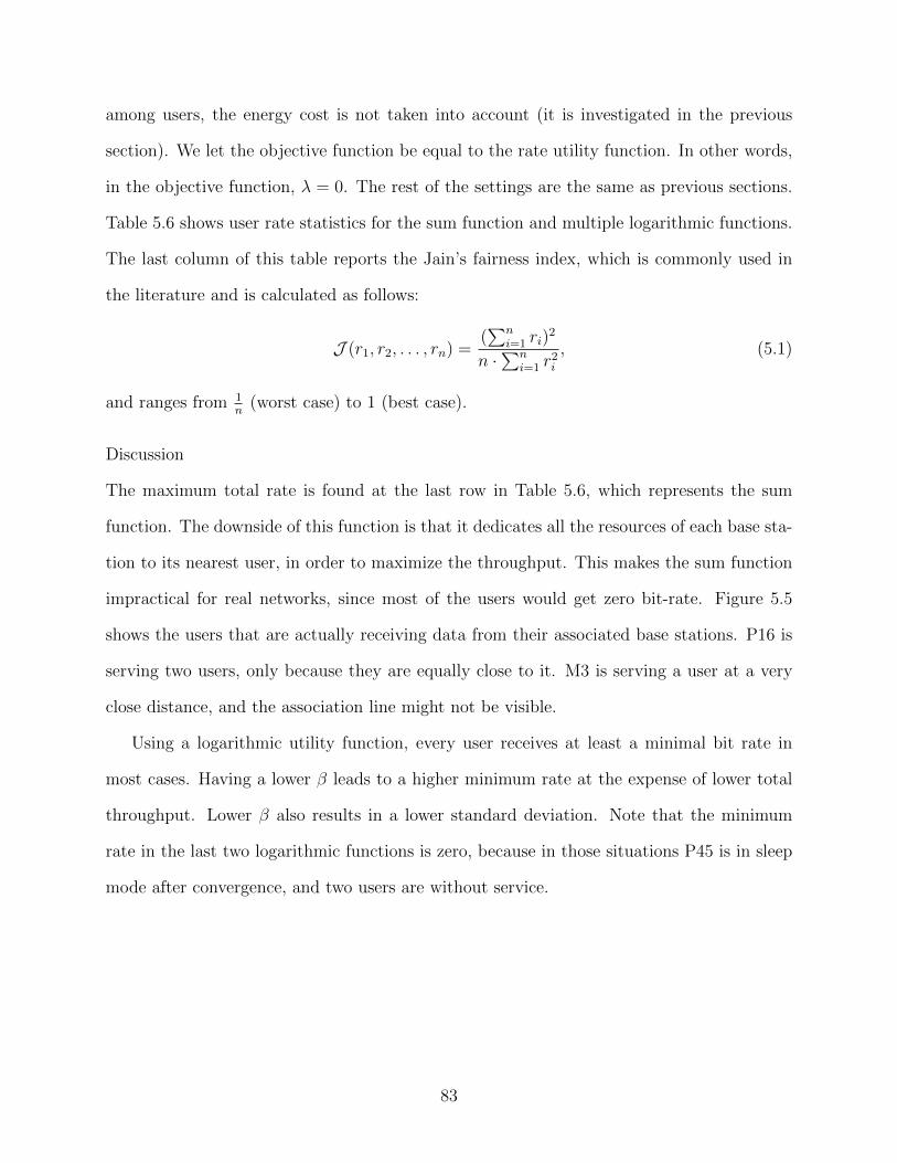
among users, the energy cost is not taken into account (it is investigated in the previous

section). We let the objective function be equal to the rate utility function. In other words,

in the objective function, λ = 0. The rest of the settings are the same as previous sections.

Table 5.6 shows user rate statistics for the sum function and multiple logarithmic functions.

The last column of this table reports the Jain’s fairness index, which is commonly used in

the literature and is calculated as follows:

J (r1, r2, . . . , rn) =(∑n

i=1 ri)2

n ·∑n

i=1 r2i

, (5.1)

and ranges from 1n

(worst case) to 1 (best case).

Discussion

The maximum total rate is found at the last row in Table 5.6, which represents the sum

function. The downside of this function is that it dedicates all the resources of each base sta-

tion to its nearest user, in order to maximize the throughput. This makes the sum function

impractical for real networks, since most of the users would get zero bit-rate. Figure 5.5

shows the users that are actually receiving data from their associated base stations. P16 is

serving two users, only because they are equally close to it. M3 is serving a user at a very

close distance, and the association line might not be visible.

Using a logarithmic utility function, every user receives at least a minimal bit rate in

most cases. Having a lower β leads to a higher minimum rate at the expense of lower total

throughput. Lower β also results in a lower standard deviation. Note that the minimum

rate in the last two logarithmic functions is zero, because in those situations P45 is in sleep

mode after convergence, and two users are without service.

83

×104

0 0.5 1 1.5 2 2.5 3

×104

0

0.5

1

1.5

2

2.5

312

3

4 5

6

7

Figure 5.5: Converged state of the network when using sum rate function. Each BS isdedicating all its resources to its nearest user. Since the cost of energy is considered zero,some of the idle pico-BSs remain on.

Table 5.6: Effect of rate utility function on user throughputs. Higher fairness (lower β)results in a lower aggregate throughput.

β Total rate Min rate Max rate Avg rate Std Dev Jain’s Ind1 569507.7 740 31636.9 5529.2 4285.2 0.610 569590.6 732.9 31637.6 5530 4285.8 0.6100 570425.2 662.3 31644.2 5538.1 4292.7 0.6200 586823.2 204.8 31651.6 5697.3 4382.4 0.61000 603490.2 0 31710.9 5859.1 4418.1 0.62000 607483.9 0 31784.9 5897.9 4496.7 0.6Sum(R) 866568.3 0 141054.5 8413.3 27021.5 0.1

84

5.5 Sleep Mode and ABS Subframes

In this section, we study the effect of pico-BS sleep mode and ABS subframes on the objec-

tive function. In other words, we show how much improvement we can achieve by letting

base stations have more options to choose from. To this end, we consider 4 different operating

modes for the network in Figure 5.1:

• A: In this mode, there is no ABS subframe, i.e. macro-BSs transmit at their

maximum power throughout the whole frame. Further, Pico-BSs are always

on and are not capable of entering sleep mode.

• B: This mode is similar to the above one, except macro-BSs can choose to

be silent in a fraction of a frame, chosen from X = {0, 1/10, 2/10, 3/10}. During

these subframes, macro-BSs refrain from transmitting any data signal. This

mode resembles LTE eICIC technology.

• C: In this mode, in addition to ABS subframes, macro-BSs are allowed to

transmit at a lower power level during ABS subframes. This power is a fraction

of the maximum RF output power, selected from Y = {0, 1/4, 1/2, 3/4}. This

mode resembles LTE feICIC technology.

• D: In the last mode, in addition to the previous features, pico-BSs are able to

enter sleep mode to further reduce the network energy consumption. This is

the default mode which is employed in Section 5.2.

In mode A, there is no Gibbs Sampling procedure and each base station only solves one

local convex optimization problem to allocate its subframes to its users. Results of mode

D are already explained in Section 5.2 and summarized in Tables 5.3 and 5.4. Table 5.7

reports the converged states of macro-BSs in mode B and mode C. In Table 5.8, we see the

performance comparison of the 4 modes, and the percentage of improvement over mode A.

85

Mode

A B C D

Obje

ctive

0

10

20

30

40

50

60

51.7

54.555.7 56.3

Figure 5.6: Maximum achieved global objective of each scenario.

Table 5.7: State of macro-BSs after convergence. B: macro-BSs have to be completely silentduring ABS subframes. C: Macro-BSs can transmit at a lower power during ABS subframes.

% M1 M2 M3 M4 M5 M6 M7ABS duration (B) 0 0 0 0 0 0 30ABS power (B) 0 0 0 0 0 0 0ABS duration (C) 30 30 30 30 30 30 30ABS power (C) 25 25 50 50 50 50 0

Discussion

In mode B, since macro-BSs are not allowed to transmit any data during ABS subframes,

having these subframes wastes resources and reduces the utility function. So except for

the macro-BS in the middle, which has multiple neighboring picocells, other macro-BSs

do not employ ABS subframes. In mode C, where macro-BSs have the freedom to choose

their output power during ABS subframes, they have all exploited this feature and gained

Table 5.8: Effect of ABS subframes and pico-BS sleep mode on global objective. By enablingeach feature, the objective is increased and the energy consumption is reduced.

Net Mode Throughput Energy Objective Objective Improvement (%)A 851492.5 1673.6 51.7 0B 874106.3 1645.4 54.5 5.5C 866705 1546.7 55.7 7.9D 866705 1519.7 56.3 8.9

86

performance improvement.

Figure 5.6 and Table 5.8 show that by enabling each feature, the objective is considerably

enhanced even in this small network. In this particular case, the throughput has remained

identical by letting the pico-BSs go to sleep mode. In general, the contribution of each of

the tested features on throughput and energy enhancement is dependent on the network

topology and can be influenced by the choice of the objective function.

5.6 Dense Deployment of Pico-BSs

In this section, we simulate 400 pico-BSs densely located in a 20x20 grid, with 1000 users

spread over the region using a PPP model. Figure 5.8 shows the network, and Figure 5.9

demonstrates its corresponding neighborhood system used by our algorithm. We want to

find the maximum objective that we can obtain by hibernating some of the pico-BSs. We

test 3 different scenarios:

• A: In this mode, all of the base stations are on and there is no coordination

between them. All they do is allocate resources to their users.

• B: In this mode, half of the base stations are on. We hibernate every other

pico-BS, which still keeps the whole area covered (Figure 5.10). By shutting

any other pico-BS down, some areas will be left uncovered.

• C: In this mode, we let our distributed algorithm choose which base stations

to power off in order to maximize the global objective.

Discussion

We can observe in Table 5.9 that the first scenario results in the lowest total throughput and

highest total energy consumption. In mode B, throughput is significantly improved due to

less interference on users. In the optimized scenario C, throughput is the highest, although

87

A B C

0

200

400

600

800

1000

1200

1400

1600

1800

874.8

1335.0

1625.1

Figure 5.7: Global objective of the grid of pico-BSs in 3 different states. A: All the BSs areon. B: Half of them are on. C: State of the network after convergence of Gibbs Sampler.

Table 5.9: Global objective of the grid of pico-BSs in 3 different states. A: All the BSsare on. B: Every other BS is on in each row and column. C: State of the network afterconvergence of Gibbs Sampler.

Throughput Energy No. of Operating PicosA 9627644.9 3520 400B 14005052.7 2620 200C 16933789.6 2732.5 225

the energy consumption is a bit more than mode B. Figure 5.7 shows that the optimized

scenario improves the objective function by 22% compared to mode B, and almost 85% over

mode A.

88

×104

0 0.5 1 1.5 2 2.5 3 3.5 4

×104

0

0.5

1

1.5

2

2.5

3

3.5

4

Figure 5.8: A 20x20 grid of pico-BSs with 1000 users.

×104

0.5 1 1.5 2 2.5 3 3.5 4

×104

0.5

1

1.5

2

2.5

3

3.5

4

Figure 5.9: Neighborhood graph of the network in Figure 5.8

89

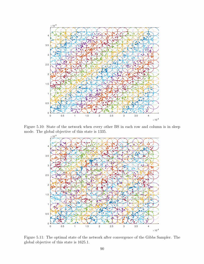
×104

0 0.5 1 1.5 2 2.5 3 3.5 4

×104

0

0.5

1

1.5

2

2.5

3

3.5

4

Figure 5.10: State of the network when every other BS in each row and column is in sleepmode. The global objective of this state is 1335.

×104

0 0.5 1 1.5 2 2.5 3 3.5 4

×104

0

0.5

1

1.5

2

2.5

3

3.5

4

Figure 5.11: The optimal state of the network after convergence of the Gibbs Sampler. Theglobal objective of this state is 1625.1.

90

5.7 Numerical Analysis of Convergence

In this section, we numerically analyze the convergence of the global objective function of

our algorithm in the network depicted in Figure 5.8.

5.7.1 Temperature Function

We evaluate 3 types of decreasing functions:

1. Logarithmic function: T (t) = T02 log(2+t)

2. Linear function: T (t) = T0(1 + t−11−tend

)

3. Quadratic function: T (t) = T0(1 + t−11−tend

)2

In the above functions, the initial temperature is set to T0 = 5. The latter two reach

zero at t = tend = 104. The iterations between two successive updates for each base station

is randomly chosen from [1, τ ] after each step, where τ = 10. Table 5.10 compares the

performance of the three mentioned functions.

Note that in order to find the global objective at any arbitrary state of the network,

each local objective function has to be evaluated once per each local neighborhood state.

For example, if a macro-BS has m adjacent macro-BSs and n adjacent pico-BSs, its local

objective function can take 2n|X × Y|m+1 different values. Given the size of state spaces of

macro-BSs and pico-BSs, and the neighborhood systems of the two networks studied in this

chapter (Figure 5.2a and Figure 5.9), the total number of local objective function evaluations

(i.e., total number of convex optimization problems) for the two networks is 123, 025 and

168, 572, respectively. However, the Gibbs Sampler may not visit all the possible states of

the networks, and therefore not all of the local objective functions have to be evaluated for

every state in their neighborhood. Table 5.10 shows how many of the convex optimization

problems were actually needed in each simulation.

91

Iteration (t)

0 1000 2000 3000 4000 5000 6000 7000 8000 9000 100000

500

1000

1500

2000

0

0.5

1

1.5

2

Global Objective

Temperature

Figure 5.12: Convergence of logarithmic temperature function

Iteration (t)

0 1000 2000 3000 4000 5000 6000 7000 8000 9000 100000

2000

0

5

Global Objective

Temperature

Figure 5.13: Convergence of linear temperature function

Table 5.10: Effect of the temperature function on convergence of the system. The logarithmicfunction only evaluates 8.3% of the local objectives and quickly finds high-energy states. Atthe end, linear and quadratic functions find better solutions.

Temperature Function Objective No. Solved % Solved Avg. No. UpdatesLogarithmic 1595.7 14018 8.3 1818.7Linear 1603.2 163468 97 1818.9Quadratic 1625.1 157873 93.7 1818.7

92

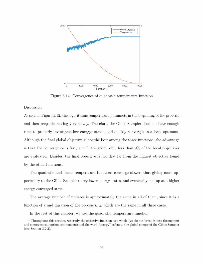
Iteration (t)

0 2000 4000 6000 8000 100000

2000

0

5

Global Objective

Temperature

Figure 5.14: Convergence of quadratic temperature function

Discussion

As seen in Figure 5.12, the logarithmic temperature plummets in the beginning of the process,

and then keeps decreasing very slowly. Therefore, the Gibbs Sampler does not have enough

time to properly investigate low energy1 states, and quickly converges to a local optimum.

Although the final global objective is not the best among the three functions, the advantage

is that the convergence is fast, and furthermore, only less than 9% of the local objectives

are evaluated. Besides, the final objective is not that far from the highest objective found

by the other functions.

The quadratic and linear temperature functions converge slower, thus giving more op-

portunity to the Gibbs Sampler to try lower energy states, and eventually end up at a higher

energy converged state.

The average number of updates is approximately the same in all of them, since it is a

function of τ and duration of the process tend, which are the same in all three cases.

In the rest of this chapter, we use the quadratic temperature function.

1 Throughout this section, we study the objective function as a whole (we do not break it into throughputand energy consumption components) and the word “energy” refers to the global energy of the Gibbs Sampler(see Section 3.2.2).

93

Table 5.11: Effect of update rate on convergence of the system. The number of iterationsbetween each two consecutive updates is randomly chosen from [1, τ ]. The table show thateven with the smallest average number of updates (198), a good objective value (1604.1) isfound at the end.

τ Objective No. Solved % Solved Avg. No. Updates100 1604.1 88153 52.3 19850 1601.4 114987 68.2 391.120 1609.5 144299 85.6 952.110 1625.1 157873 93.7 1818.75 1613.6 163925 97.2 3334.11 1622.7 167838 99.6 10000

5.7.2 Update Rate

In this section we investigate the effect of update rate of base station states on the final

global objective. The number of iterations in each simulation is 104. Remember that how

frequently a BS is updated depends on the parameter τ . A higher value of τ results in fewer

updates.

Discussion

Table 5.11 implies that having more updates does not always guarantee higher global objec-

tive values. In the last row, each BS is updated at each iteration, and 99.6% of the possible

states of the network have been evaluated, yet the final global objective is less than the one

with τ = 10. In the first row, on the other hand, only half of the states are investigated,

and with average of 198 updates per BS, a reasonably good global objective is found. In

general, this parameter should be tuned in conjunction with the duration parameter tend,

since together they determine the number of updates of each BS.

5.7.3 Initial Temperature

This section studies how the initial temperature affects the converged global objective. We

use the quadratic function with tend = 104 and τ = 10.

94

Table 5.12: Effect of the initial temperature on convergence of the system. Starting fromhigher temperatures does not necessarily lead to higher final objective values, although itmakes the algorithm consider more possibilities.

T0 Objective No. Solved % Solved Avg. No. Updates1 1611.3 31602 18.7 1818.33 1606.7 132436 78.6 1818.45 1625.1 157873 93.7 1818.710 1610.3 166687 98.9 1818.1100 1618.8 168484 99.9 1818.6

Table 5.13: Effect of the duration of the Gibbs Sampling process on the final global objectivein grid of pico-BSs. Longer runtimes lead to better solutions.

tend Objective No. Solved % Solved Avg. No. Updates100 1555.4 23217 13.8 18500 1603.9 61235 36.3 90.81000 1607.7 88250 52.4 182.15000 1615.1 144511 85.7 909.410000 1625.1 157873 93.7 1818.7

Discussion

Table 5.12 suggests that starting from a very high temperature does not necessarily improve

the final value. It may even cause the Gibbs Sampler to waste its time searching for states

that are unlikely to be optimal, and have less time to try states with a higher potential to be

the global maximum. A fairly good global objective is found with T0 = 1, with only solving

18.7% of the convex optimizations across the network.

5.7.4 Duration

Finally, we investigate the effect of the number of iterations of the algorithm (tend) on the

final global objective. We use quadratic functions that start at T0 = 5 and reach zero at

different tend values.

Discussion

Table 5.13 shows that by increasing the length of the process, we get improved results, which

is intuitively true. It should be noted that even though the best global objective is found

95

Number of iterations

10 2 10 3 10 4

Fin

al g

lob

al o

bje

ctive

1550

1560

1570

1580

1590

1600

1610

1620

1630

Figure 5.15: Semi-log plot of effect of duration of the algorithm on the final global objective.

Table 5.14: Effect of duration of Gibbs Sampling on the final global objective in the HetNetof Figure 5.1. Because the network is small, a few number of updates is enough to reach theoptimal solution.

tend Objective No. Solved % Solved Avg. No. Updates50 55.9 1622 1.3 8.2100 56.3 2597 2.1 17.31000 56.3 12229 9.9 180.1

96

with 10000 iterations, using one tenth of this number we can still get a good global objective

which is only 1.1% less than the highest value. The semi-log plot of the objective values in

Table 5.13 is presented in Figure 5.15.

From the tables and plots in this section, we conclude that there is a trade-off between

the speed of convergence and the quality of the final global objective. In general, the more

updates per BS, which can be achieved by a larger tend or a smaller τ , results in a better

converged state.

Additionally, choosing the right parameters for the temperature function depends on the

topology of the network. In Table 5.14, we see the effect of the duration of the algorithm on

the final global objective in the network of Section 5.2. Since the neighborhood graph of this

network (Figure 5.2a) is much smaller than that of the pico-BS grid scenario (Figure 5.9),

the effect of each BS update propagates throughout the network faster, and fewer updates

are needed to find the optimal state. Table 5.14 shows that by solving only 2.1% of the

123025 convex optimization problems, the best state has been found.

97

Chapter 6

Conclusion

In this work, we developed a distributed algorithm to balance the trade-off between energy

consumption and throughput of heterogeneous cellular networks. Our algorithm achieves

this by putting underutilized pico base stations in standby mode and adjusting the ratio of

almost blank subframes in individual macro base stations, in order to minimize the inter-

ference on pico-BS users. In addition to the ratio of ABS subframes, our algorithm allows

macro-BSs to serve their users at a lower output power, which is assigned to individual

macro-BSs in an optimal fashion that maximizes the aggregate network utility. An impor-

tant feature of the proposed algorithm is its distributed manner, which is achieved by using

Gibbs Sampling. To the best of our knowledge, this is the first method proposed to power off

pico-BSs and adjust output power of ABS subframes in a decentralized way. The simulation

results show that our algorithm has reduced the energy consumption by more than 9% in

the HetNet described in Section 5.1. Moreover, the global objective is increased by 22% in

the picocell grid depicted in Figure 5.8.

6.1 Thesis Summary

In Chapter 1, we explained the problem and presented the goal of the research. We men-

tioned the rapid growth of cellular networks, and pointed out two unavoidable consequences

of this expansion. One is the energy concern that emerges as a result of more cells in Het-

Nets, which is a crucial consideration in deploying pico-BSs. The other is the importance of

self-optimization of network parameters and minimizing manual network configuration man-

agement. Also, we emphasized the tendency of network operators to simplify the structure

of modern cellular networks, and expressed our motivation towards designing a distributed

98

algorithm that is run by base stations without requiring a separate coordinator entity.

Then, in Chapter 2, we reviewed the methods of associating mobile users to cellular

base stations. We explained the static RSRP-based method, as well as load-aware schemes.

Range expansion was mentioned as the mechanism provided by LTE networks to perform

load-balancing and offload macrocell users to picocells. Chapter 2 also elaborated different

types of interference. This includes the interference on cell-edge users, the interference

imposed by macro-BSs to small cells, and the interference imposed by femto-BSs on macrocell

users that are not registered in the closed subscription group of femtocells. Then the inter-

cell interference coordination schemes were reviewed. Frequency domain separation is one

such method, although not typically used in LTE networks where frequency reuse factor is

1. Also, time domain and power allocation schemes were discussed, and ABS subframes

of eICIC and low-power ABS subframes of feICIC were explained as examples of them. A

review of different types of self-organization in cellular networks is provided in Chapter 2,

and the difference between centralized and distributed approaches is scrutinized.

Chapter 3 contains theoretical aspects of the optimization techniques in our work. We

briefly discussed convex optimization problems, which are used in our meta-optimization

to solve the local resource allocation in each cell. Then we named some common discrete

optimization techniques, and laid out their shortcomings for our problem. Gibbs Sampling

was described after reviewing some basic definitions, and justified as a suitable optimization

method for our problem. At the end of the chapter, using an example, we demonstrated how

Gibbs Sampling can be utilized to solve a network-wide optimization problem, where each

node has a local objective, and the network can be represented as a Markov random field.

In Chapter 4, we reiterated our design goals, and specified the assumptions made in our

design. Then we defined a neighborhood system on the graph of base stations in the network,

in a way that they constitute a Markov random field. We formulated a rate utility function

to be maximized, an energy cost function to be minimized, and a global objective function

99

to balance the two conflicting goals. We then presented our iterative method, which requires

limited information exchange between neighboring BSs and drives the system to the optimal

state.

Finally, we simulated the algorithm and examined the performance of the proposed

method in Chapter 5 and evaluated the effect of each parameter. Numerical studies showed

that the algorithm can very quickly converge to near-optimal states, and find the optimal

solution in a reasonable amount of time. We demonstrated how network operators are able

to balance the throughput-energy trade-off in our method by tuning the objective function.

The level of fairness is also showed to be tunable by tweaking the rate utility function.

Then we showed that considerable energy saving is achievable by turning off some pico-BSs

without losing much throughput.

We simulated two network topologies, one HetNet comprising 7 macro-BSs and 12 pico-

BSs, and one grid of pico-BSs. In a real scenario, due to the distributed manner of the

proposed method, each BS separately solves its own convex optimizations, so the computa-

tional complexity of the global algorithm is not directly a function of number of BSs. In the

simulations, all the computations are performed on one PC with limited resources. Consid-

ering the fact that analyzing each parameter requires many simulations, we had limitations

on the size of the networks under study. Nevertheless, we observed promising outcomes even

in the small-scale HetNet scenario.

6.2 Future Work

Several lines of research can be pursued by expanding the ideas of this thesis. In the following,

we suggest some of the interesting areas for future investigation:

• Load balancing: In our proposed method, mobile users associate with the base station

with the maximum reference signal received power. For future studies, we can incorporate

user association to perform load balancing using the range expansion concept. This can

100

be achieved using the same Gibbs Sampling technique, by adding cell selection bias to

state space of base stations. This way, instead of having only 2 states (on / off), pico-BSs

can have multiple states each of which indicates a specific coverage range.

• Multiple frequency channels: The algorithm can be further extended by supporting

multiple frequency channels. Then for each macro-BS, we can maintain a set of states for

ABS duration and ABS power ratios per channel. Subframes would also be allocated to

users separately on each channel. This makes it more likely for users with high interference

on one channel to be served interference-free on another channel.

• Integer number of subframes: Another enhancement can take place in the locally

solved resource allocation stage of the algorithm. Right now we allocate a real fraction of

the subframes to each user, and this makes it possible for each base station to optimally

allocate subframes to its users by solving a convex optimization problem. However, in

cellular networks, the number of subframes of a frame is predefined, and they cannot

be partially assigned to users. This makes the assignment problem an integer linear

problem that cannot be solved by convex solvers. This thesis has been concentrated on

the distributed part of the optimization. Moreover, the assumption of real-valued fraction

of subframes has been exploited in the literature. Nonetheless, this can be achieved as a

future work, for example by linear programming relaxation.

• Fast-changing environments: An intriguing future research would be to investigate

the performance of Gibbs Sampling in rapidly-changing environments. Our algorithm

assumes that the arrival and departure rates of users are slow and the users stay relatively

stationary during the short convergence period. It would be interesting to study the

extent to which user movements can affect the performance of Gibbs Sampling. Next, we

can relax the mentioned assumption by adapting the Gibbs Sampler to a dynamic user

population.

101

Bibliography

[1] Femtocell and microcells. Available online at https://www.repeaterstore.com/

pages/femtocell-and-microcell.

[2] Path loss. Available online at https://en.wikipedia.org/wiki/Path_loss.

[3] Saddle point. Available online at https://en.wikipedia.org/wiki/Saddle_point.

[4] Simulated annealing. Available online at https://en.wikipedia.org/wiki/

Simulated_annealing.

[5] Heterogeneous networks - securing excellent mobile broadband user experience, every-

where. Technical report, Ericsson, 2014.

[6] Ericsson mobility report: On the pulse of the networked society. Technical report,

Ericsson, 2015.

[7] 3GPP. Evolved Universal Terrestrial Radio Access (E-UTRA) and Evolved Universal

Terrestrial Radio Access Network (E-UTRAN); Overall description; Stage 2. TS 36.300,

3rd Generation Partnership Project (3GPP), 03 2011.

[8] 3GPP. Evolved Universal Terrestrial Radio Access (E-UTRA); Mobility enhancements

in heterogeneous networks. TR 36.839, 3rd Generation Partnership Project (3GPP), 06

2011.

[9] 3GPP. UTRAN Iub interface Node B Application Part (NBAP) signalling. TS 25.433,

3rd Generation Partnership Project (3GPP), 06 2011.

[10] 3GPP. LTE; E-UTRAN; X2 Application Protocol (Release 12). Technical Report

36.423, 3rd Generation Partnership Project (3GPP), 2015.

102

[11] Ali Abbasi and Majid Ghaderi. Online algorithms for energy cost minimization in

cellular networks. In Proceedings of IEEE 22nd International Symposium of Quality of

Service (IWQoS), pages 302–307. IEEE, 2014.

[12] Imran Ashraf, Federico Boccardi, and Lester Ho. Sleep mode techniques for small cell

deployments. IEEE Communications Magazine, 49(8):72–79, 2011.

[13] Wei Bao and Ben Liang. Structured spectrum allocation and user association in hetero-

geneous cellular networks. In Proceedings of IEEE INFOCOM, pages 1069–1077. IEEE,

2014.

[14] Murat Bilgic. Who needs lte small cells first? Technical report, EXFO, 2013.

[15] Sem C Borst, Mihalis G Markakis, and Iraj Saniee. Nonconcave utility maximiza-

tion in locally coupled systems, with applications to wireless and wireline networks.

IEEE/ACM Transactions on Networking, 22(2):674–687, 2014.

[16] Claudio Bottai, Claudio Cicconetti, Arianna Morelli, Michele Rosellini, and Christian

Vitale. Energy-efficient user association in extremely dense small cells. In Proceedings

of the European Conference on Networks and Communications (EuCNC14), 2014.

[17] Stephen Boyd and Lieven Vandenberghe. Convex optimization. Cambridge university

press, 2004.

[18] Pierre Bremaud. Markov chains: Gibbs fields, Monte Carlo simulation, and queues,

volume 31. Springer Science & Business Media, 2013.

[19] Chung Shue Chen and Francois Baccelli. Self-optimization in mobile cellular networks:

Power control and user association. In Proceedings of IEEE International Conference

on Communications (ICC), pages 1–6. IEEE, 2010.

103

[20] Xiaohui Chen, Wenqing Cheng, Wei Yuan, Wei Liu, and Jing Xu. Joint optimization of

channel allocation and ap association in variable channel-width wlans. In Proceedings of

IEEE Wireless Communications and Networking Conference (WCNC), pages 345–350.

IEEE, 2013.

[21] Michal Cierny, Haining Wang, Risto Wichman, Zhi Ding, and Carl Wijting. On number

of almost blank subframes in heterogeneous cellular networks. IEEE Transactions on

Wireless Communications, 12(10):5061–5073, 2013.

[22] Cisco Visual Networking Index Cisco. Global mobile data traffic forecast update, 2014–

2019. white paper, 2015.

[23] Steven Corroy, Laetitia Falconetti, and Rudolf Mathar. Cell association in small het-

erogeneous networks: Downlink sum rate and min rate maximization. In Proceedings of

IEEE Wireless Communications and Networking Conference (WCNC), pages 888–892.

IEEE, 2012.

[24] Pierre Coucheney, Corinne Touati, and Bruno Gaujal. Fair and efficient user-network

association algorithm for multi-technology wireless networks. In Proceedings of IEEE

INFOCOM, pages 2811–2815. IEEE, 2009.

[25] Frederico RB Cruz, Geraldo Robson Mateus, and J MacGregor Smith. A branch-

and-bound algorithm to solve a multi-level network optimization problem. Journal of

Mathematical Modelling and Algorithms, 2(1):37–56, 2003.

[26] Sajal K Das and Sanjoy K Sen. A new location update strategy for cellular networks

and its implementation using a genetic algorithm. In Proceedings of the 3rd annual

ACM/IEEE international conference on Mobile computing and networking, pages 185–

194. ACM, 1997.

[27] Suman Das, Harish Viswanathan, and Gee Rittenhouse. Dynamic load balancing

104

through coordinated scheduling in packet data systems. In Proceedings of IEEE IN-

FOCOM, volume 1, pages 786–796. IEEE, 2003.

[28] Antonio De Domenico, Valentin Savin, and Dimitri Ktenas. A backhaul-aware cell selec-

tion algorithm for heterogeneous cellular networks. In Proceedings of IEEE 24th Inter-

national Symposium on Personal Indoor and Mobile Radio Communications (PIMRC),

pages 1688–1693. IEEE, 2013.

[29] Supratim Deb, Pantelis Monogioudis, Jerzy Miernik, and James P Seymour. Algorithms

for enhanced inter-cell interference coordination (eicic) in lte hetnets. IEEE/ACM

Transactions on Networking (TON), 22(1):137–150, 2014.

[30] Bjorn Debaillie, Alexandre Giry, Manuel J Gonzalez, Laurent Dussopt, Min Li, Dieter

Ferling, and Vito Giannini. Opportunities for energy savings in pico/femto-cell base-

stations. In Future Network & Mobile Summit (FutureNetw), pages 1–8. IEEE, 2011.

[31] Gianni A Di Caro, Frederick Ducatelle, and Luca M Gambardella. Ant colony optimiza-

tion for routing in mobile ad hoc networks in urban environments. Technical report,

Dalle Molle Institute for Artificial Intelligence, Manno, Switzerland, 2008.

[32] Russell C Eberhart and Yuhui Shi. Particle swarm optimization: developments, applica-

tions and resources. In Proceedings of the 2001 Congress on Evolutionary Computation,

volume 1, pages 81–86. IEEE, 2001.

[33] Ahmed Elwhishi, Issmail Ellabib, and Idris El-Feghi. Ant colony optimization for loca-

tion area planning in cellular networks.

[34] Juan Espino and Jan Markendahl. Analysis of macro–femtocell interference and impli-

cations for spectrum allocation. In Proceedings of IEEE 20th International Symposium

on Indoor and Mobile Radio Communications, pages 2208–2212. IEEE, 2009.

105

[35] Konstantinos P Ferentinos and Theodore A Tsiligiridis. Adaptive design optimization

of wireless sensor networks using genetic algorithms. Computer Networks, 51(4):1031–

1051, 2007.

[36] Dariush Fooladivanda and Catherine Rosenberg. Joint resource allocation and user

association for heterogeneous wireless cellular networks. IEEE Transactions on Wireless

Communications, 12(1):248–257, 2013.

[37] Joseph RL Fournier and Samuel Pierre. Assigning cells to switches in mobile networks

using an ant colony optimization heuristic. Computer communications, 28(1):65–73,

2005.

[38] Fabio Garzia, Cristina Perna, Roberto Cusani, et al. Optimization of umts network

planning using genetic algorithms. Communications and Network, 2(03):193, 2010.

[39] Jagadish Ghimire and Catherine Rosenberg. Resource allocation, transmission coordi-

nation and user association in heterogeneous networks: a flow-based unified approach.

IEEE Transactions on Wireless Communications, 12(3):1340–1351, 2013.

[40] Fred Glover. Tabu search: A tutorial. Interfaces, 20(4):74–94, 1990.

[41] Paulo RL Gondim. Genetic algorithms and the location area partitioning problem in

cellular networks. In Proceedings of IEEE Vehicular Technology Conference, Mobile

Technology for the Human Race, volume 3, pages 1835–1838. IEEE, 1996.

[42] Didem Gozupek, Gaye Genc, and Cem Ersoy. Channel assignment problem in cellu-

lar networks: A reactive tabu search approach. In Proceedings of 24th International

Symposium on Computer and Information Sciences (ISCIS), pages 298–303, 2009.

[43] Vu Nguyen Ha and Long Bao Le. Distributed base station association and power con-

trol for heterogeneous cellular networks. IEEE Transactions on Vehicular Technology,

63(1):282–296, 2014.

106

[44] Jin-Kao Hao, Raphael Dorne, and Philippe Galinier. Tabu search for frequency assign-

ment in mobile radio networks. Journal of heuristics, 4(1):47–62, 1998.

[45] Ekram Hossain, Mehdi Rasti, Hina Tabassum, and Amr Abdelnasser. Evolution toward

5g multi-tier cellular wireless networks: An interference management perspective. IEEE

Wireless Communications, 21(3):118–127, 2014.

[46] MA Imran, E Katranaras, G Auer, O Blume, V Giannini, I Godor, Y Jading, M Olsson,

D Sabella, P Skillermark, et al. Energy efficiency analysis of the reference systems, areas

of improvements and target breakdown. Technical report, Tech. Rep. ICT-EARTH

deliverable, 2011.

[47] Jie Jia, Jian Chen, Guiran Chang, and Zhenhua Tan. Energy efficient coverage control

in wireless sensor networks based on multi-objective genetic algorithm. Computers &

Mathematics with Applications, 57(11):1756–1766, 2009.

[48] Satya Krishna Joshi, Pradeep Chathuranga Weeraddana, Marian Codreanu, and Matti

Latva-Aho. Weighted sum-rate maximization for miso downlink cellular networks via

branch and bound. IEEE Transactions on Signal Processing, 60(4):2090–2095, 2012.

[49] Hany Kamal, Marceau Coupechoux, and Philippe Godlewski. A tabu search dsa al-

gorithm for reward maximization in cellular networks. In Proceedings of IEEE 6th

International Conference on Wireless and Mobile Computing, Networking and Commu-

nications (WiMob), pages 40–45. IEEE, 2010.

[50] Irene Katzela and Mahmoud Naghshineh. Channel assignment schemes for cellular

mobile telecommunication systems: A comprehensive survey. IEEE Personal Commu-

nications, 3(3):10–31, 1996.

[51] Bruno Kauffmann, Francois Baccelli, Augustin Chaintreau, Vivek Mhatre, Konstantina

Papagiannaki, and Christophe Diot. Measurement-based self organization of interfering

107

802.11 wireless access networks. In Proceedings of IEEE INFOCOM, pages 1451–1459.

IEEE, 2007.

[52] Turkan Ahmed Khaleel and Manar Younis Ahmed. Using intelligent water drops al-

gorithm for optimisation routing protocol in mobile ad–hoc networks. International

Journal of Reasoning-based Intelligent Systems, 4(4):227–234, 2012.

[53] Aamod Khandekar, Naga Bhushan, Ji Tingfang, and Vieri Vanghi. Lte-advanced: Het-

erogeneous networks. In Proceedings of European Wireless Conference (EW), pages

978–982. IEEE, 2010.

[54] Raghavendra V Kulkarni and Ganesh Kumar Venayagamoorthy. Particle swarm opti-

mization in wireless-sensor networks: A brief survey. IEEE Transactions on Systems,

Man, and Cybernetics, Part C: Applications and Reviews, 41(2):262–267, 2011.

[55] NM Latiff, Charalampos C Tsimenidis, and Bayan S Sharif. Energy-aware clustering

for wireless sensor networks using particle swarm optimization. In Proceedings of IEEE

18th International Symposium on Personal, Indoor and Mobile Radio Communications,

PIMRC, pages 1–5. IEEE, 2007.

[56] Xiaohang Li, Xiaojun Tang, Chih-Chun Wang, and Xiaojun Lin. Gibbs-sampling-based

optimization for the deployment of small cells in 3g heterogeneous networks. In Pro-

ceedings of IEEE 11th International Symposium on Modeling & Optimization in Mobile,

Ad Hoc & Wireless Networks (WiOpt), pages 444–451. IEEE, 2013.

[57] Ritesh Madan, Jaber Borran, Ashwin Sampath, Naga Bhushan, Aamod Khandekar,

and Tingfang Ji. Cell association and interference coordination in heterogeneous lte-a

cellular networks. IEEE Journal on Selected Areas in Communications, 28(9):1479–

1489, 2010.

108

[58] Chiu Y Ngo and Victor OK Li. Fixed channel assignment in cellular radio net-

works using a modified genetic algorithm. IEEE Transactions on Vehicular Technology,

47(1):163–172, 1998.

[59] LEI NIU and MUHAMMAD SALMAN. Resource allocation and power control for

device-to-device (d2d) communication. Master’s thesis, CHALMERS UNIVERSITY

OF TECHNOLOGY, Gteborg, Sweden, 2013.

[60] Nasr Obaid and Andreas Czylwik. Energy efficiency analysis of dense picocell deploy-

ments. In Proceedings of 18th International OFDM Workshop (InOWo’14), pages 1–6.

VDE, 2014.

[61] Jinyoung Oh and Youngnam Han. Cell selection for range expansion with almost blank

subframe in heterogeneous networks. In Proceedings of IEEE 23rd International Sympo-

sium on Personal Indoor and Mobile Radio Communications (PIMRC), pages 653–657.

IEEE, 2012.

[62] Olav Østerbø and Ole Grøndalen. Benefits of self-organizing networks (son) for mobile

operators. Journal of Computer Networks and Communications, 2012, 2012.

[63] Samuel Pierre and Fabien HoueTo. A tabu search approach for assigning cells to switches

in cellular mobile networks. Computer Communications, 25(5):464–477, 2002.

[64] Athul Prasad, Andreas Maeder, and Chenghock Ng. Energy efficient small cell activa-

tion mechanism for heterogeneous networks. In Proceedings of IEEE Globecom Work-

shops (GC Wkshps), pages 754–759. IEEE, 2013.

[65] Alejandro Quintero and Samuel Pierre. On the design of large-scale cellular mobile

networks using multi-population memetic algorithms. In Engineering Evolutionary In-

telligent Systems, pages 353–377. Springer, 2008.

109

[66] Aimin Sang, Xiaodong Wang, Mohammad Madihian, and Richard D Gitlin. Coor-

dinated load balancing, handoff/cell-site selection, and scheduling in multi-cell packet

data systems. Wireless Networks, 14(1):103–120, 2008.

[67] Sunil Srinivasa and Martin Haenggi. Path loss exponent estimation in large wireless

networks. In Information Theory and Applications Workshop, pages 124–129. IEEE,

2009.

[68] David J Strauss. Hammersley–clifford theorem. Encyclopedia of Statistical Sciences,

1983.

[69] Rahul Urgaonkar. Optimal resource allocation and cross-layer control in cognitive and

cooperative wireless networks. University of Southern California, 2011.

[70] Rui Wang and Yinggang Du. Het-net throughput analysis with picocell interference

cancellation. In Proceedings of IEEE International Conference on Communications

Workshops (ICC), pages 1–6. IEEE, 2011.

[71] Zhang Yangyang, J Chunlin, Yuan Ping, LI Manlin, Wang Chaojin, Wang Guangxing,

et al. Particle swarm optimization for base station placement in mobile communication.

In Proceedings of IEEE International Conference on Networking, Sensing and Control,

volume 1, pages 428–432. IEEE, 2004.

[72] Qiaoyang Ye, Mazin Al-Shalashy, Constantine Caramanis, and Jeffrey G Andrews.

On/off macrocells and load balancing in heterogeneous cellular networks. In Proceedings

of IEEE Global Communications Conference (GLOBECOM), pages 3814–3819. IEEE,

2013.

110