university of calgary markov chain analysis of web cache
TRANSCRIPT

UNIVERSITY OF CALGARY
Markov Chain Analysis of Web Cache Systems
under TTL-based Consistency
by
Hazem Anwar Gomaa
A THESIS
SUBMITTED TO THE FACULTY OF GRADUATE STUDIES
IN PARTIAL FULFILLMENT OF THE REQUIREMENTS FOR THE
DEGREE OF DOCTOR OF PHILOSOPHY
DEPARTMENT OF ELECTRICAL AND COMPUTER ENGINEERING
CALGARY, ALBERTA
April, 2013
c© Hazem Anwar Gomaa 2013

Abstract
Caching plays a crucial role in improving Web-based services. The basic idea of Web
caching is to satisfy the user’s requests from a nearby cache, rather than a faraway
origin server (OS). This reduces the user’s perceived latency, the load on the OS, and
the network bandwidth consumption.
This dissertation introduces a new analytical model for estimating the cache hit
ratio as a function of time. The cache may not reach the steady state hit ratio
(SSHR) when the number of Web objects, object popularity, and/or caching resources
themselves are subject to change. Hence, the only way to quantify the hit ratio
experienced by users is to calculate the instantaneous hit ratio (IHR). The proposed
analysis considers a single cache with either infinite or finite capacity. For a cache
with finite capacity, two replacement policies are considered: first-in-first-out (FIFO)
and least recently used (LRU). In addition, the proposed analysis accounts for the use
of two variants of the time-to-live (TTL) weak consistency mechanism. The first is
the typical TTL (TTL-T), specified in the HTTP/1.1 protocol, where expired objects
are refreshed using conditional GET requests. The second is TTL immediate ejection
(TTL-IE) whereby objects are ejected as soon as they expire. Based on the insights
from the analysis, a new replacement policy named frequency-based-FIFO (FB-FIFO)
is proposed. The results show that FB-FIFO achieves a better IHR than FIFO and
LRU.
Furthermore, the analytical model of a single cache is extended for characteriz-
ing the instantaneous average hit distance (IAHD) of two cooperative Web caching
ii

systems, distributed and hierarchical. In these systems, the analysis considers fixed
caches that are always connected to the network, and temporary caches that ran-
domly join and leave the network. In the distributed cache system, the analysis
considers caches that cooperate via Internet cache protocol (ICP). In the hierarchical
cache system, the analysis accounts for two sharing protocols: leave copy everywhere
(LCE) and promote cached objects (PCO), which is a new protocol that is introduced
in this dissertation. The results show that PCO outperforms LCE in terms of the
IAHD, especially under TTL-T.
iii

Acknowledgements
I am deeply indebted to my supervisor, Dr. Geoffrey Messier, for his guidance,
support, and advice throughout my dissertation. Dr. Messier helped me to identify
research problems and provided me with his full support in pursuing my ideas. Dr.
Messier’s way of thinking and dealing with difficulties positively influenced not only
my dissertation, but also my personal life.
I thank my co-supervisor, Dr. Robert Davies, for his ongoing discussions about
my research and his assistance in providing funding to support my research.
I would like to express my sincere gratitude to Dr. Carey Williamson for his useful
comments and crucial feedbacks that helped me a lot to improve the quality of my
dissertation.
I thank TRLabs (Telecommunications Research Laboratories, Alberta) who pro-
vided financial support through their scholarship, which allowed me to pursue my
degree.
I thank all my colleagues in FISH Lab for their ongoing help. I also would like to
thank Martin F. Arlitt for providing technical materials that helped me during my
research.
Finally, I deeply appreciate and give my heartfelt thanks to my parents, Fatma
Mohamad and Anwar Gomaa, for their love and support, and my uncle, Dr. Ismail
Gomaa, for encouraging me to continue my graduate studies.
iv

Dedication
To my lovely wife, Mayada Younes.
To my beautiful daughter, Jumana Gomaa.
v

Table of Contents
Abstract . . . . . . . . . . . . . . . . . . . . . . . . . . . . . . . . . . . . . iiAcknowledgements . . . . . . . . . . . . . . . . . . . . . . . . . . . . . . . ivDedication . . . . . . . . . . . . . . . . . . . . . . . . . . . . . . . . . . . . vTable of Contents . . . . . . . . . . . . . . . . . . . . . . . . . . . . . . . . viList of Tables . . . . . . . . . . . . . . . . . . . . . . . . . . . . . . . . . . ixList of Figures and Illustrations . . . . . . . . . . . . . . . . . . . . . . . . xList of Symbols, Abbreviations, Nomenclature . . . . . . . . . . . . . . . . xiii1 Introduction . . . . . . . . . . . . . . . . . . . . . . . . . . . . . . . . 11.1 Proposed Web Cache Systems . . . . . . . . . . . . . . . . . . . . . . 3
1.1.1 Single Cache System (SCS) . . . . . . . . . . . . . . . . . . . 31.1.2 Hierarchical Cache System (HCS) . . . . . . . . . . . . . . . . 61.1.3 Distributed Cache System (DCS) . . . . . . . . . . . . . . . . 71.1.4 Temporary Cache (TC) . . . . . . . . . . . . . . . . . . . . . . 9
1.2 Evaluation Methodology . . . . . . . . . . . . . . . . . . . . . . . . . 131.3 Motivations and List of Contributions . . . . . . . . . . . . . . . . . . 181.4 Dissertation Roadmap . . . . . . . . . . . . . . . . . . . . . . . . . . 202 Background . . . . . . . . . . . . . . . . . . . . . . . . . . . . . . . . 212.1 HTTP and Cache Consistency Mechanisms . . . . . . . . . . . . . . . 212.2 Cache Replacement Policies . . . . . . . . . . . . . . . . . . . . . . . 262.3 Access Pattern Characteristics . . . . . . . . . . . . . . . . . . . . . . 282.4 SCS Analytical Models in the Literature . . . . . . . . . . . . . . . . 302.5 Research on Hierarchical Cache Systems . . . . . . . . . . . . . . . . 32
2.5.1 HCS Sharing Protocols . . . . . . . . . . . . . . . . . . . . . . 332.5.2 HCS Analytical Models in the Literature . . . . . . . . . . . . 35
2.6 Research on Distributed Caching Systems . . . . . . . . . . . . . . . 362.6.1 DCS Sharing Protocols . . . . . . . . . . . . . . . . . . . . . . 362.6.2 DCS Analytical Models in the Literature . . . . . . . . . . . . 38
2.7 Research on Mobile Cache Systems . . . . . . . . . . . . . . . . . . . 393 Analysis of the Single Cache System (SCS) . . . . . . . . . . . . . . . 433.1 Analysis Assumptions . . . . . . . . . . . . . . . . . . . . . . . . . . 443.2 Analysis of Infinite Cache . . . . . . . . . . . . . . . . . . . . . . . . 46
3.2.1 Infinite Cache under NEM . . . . . . . . . . . . . . . . . . . . 473.2.2 Infinite Cache under TTL-IE . . . . . . . . . . . . . . . . . . 483.2.3 Infinite Cache under TTL-T . . . . . . . . . . . . . . . . . . . 50
3.3 Analysis of Perfect-LFU . . . . . . . . . . . . . . . . . . . . . . . . . 523.4 Analysis of FIFO . . . . . . . . . . . . . . . . . . . . . . . . . . . . . 53
3.4.1 FIFO Cache under NEM . . . . . . . . . . . . . . . . . . . . . 543.4.2 FIFO Cache under TTL-IE . . . . . . . . . . . . . . . . . . . 573.4.3 FIFO Cache under TTL-T . . . . . . . . . . . . . . . . . . . . 59
3.5 Analysis of LRU . . . . . . . . . . . . . . . . . . . . . . . . . . . . . . 613.5.1 LRU Cache under NEM . . . . . . . . . . . . . . . . . . . . . 613.5.2 LRU Cache under TTL-IE . . . . . . . . . . . . . . . . . . . . 62
vi

3.5.3 LRU Cache under TTL-T . . . . . . . . . . . . . . . . . . . . 633.6 Generalized Analysis of a Non-stationary Access Pattern . . . . . . . 65
3.6.1 Generalized Analysis of Infinite Cache . . . . . . . . . . . . . 653.6.2 Generalized Analysis of FIFO and LRU . . . . . . . . . . . . . 67
3.7 FB-FIFO Replacement Policy . . . . . . . . . . . . . . . . . . . . . . 673.8 Evaluation of the IHR under NEM and TTL-IE . . . . . . . . . . . . 72
3.8.1 Evaluation of Replacement Policies under a Stationary AccessPattern . . . . . . . . . . . . . . . . . . . . . . . . . . . . . . 74
3.8.2 Evaluation of Replacement Policies under a Non-stationary Ac-cess Pattern . . . . . . . . . . . . . . . . . . . . . . . . . . . . 80
3.9 Evaluation of the SSHR under TTL-IE and TTL-T . . . . . . . . . . 833.10 Summary . . . . . . . . . . . . . . . . . . . . . . . . . . . . . . . . . 884 Analysis of the Hierarchical Cache System (HCS) . . . . . . . . . . . 904.1 Evaluation Metrics and Assumptions . . . . . . . . . . . . . . . . . . 914.2 Analysis of LCE . . . . . . . . . . . . . . . . . . . . . . . . . . . . . . 934.3 Promote Cached Object (PCO) . . . . . . . . . . . . . . . . . . . . . 95
4.3.1 PCO Motivation . . . . . . . . . . . . . . . . . . . . . . . . . 954.3.2 PCO Protocol under TTL-IE or TTL-T . . . . . . . . . . . . 974.3.3 Analysis of PCO under TTL-IE . . . . . . . . . . . . . . . . . 97
4.4 Analysis of Temporary Leaf Caches (TLCs) . . . . . . . . . . . . . . 994.4.1 TLCs Network Model and Assumptions . . . . . . . . . . . . . 994.4.2 TLCs Analysis . . . . . . . . . . . . . . . . . . . . . . . . . . 102
4.5 Cache Performance Evaluation . . . . . . . . . . . . . . . . . . . . . . 1044.5.1 Evaluation of the SSAHD under NEM and TTL-IE . . . . . . 1064.5.2 Evaluation of the SSAHD under TTL-T . . . . . . . . . . . . 1084.5.3 Evaluation of the IAHD under NEM . . . . . . . . . . . . . . 1104.5.4 Impact of TLCs under NEM and TTL-IE . . . . . . . . . . . 113
4.6 Summary . . . . . . . . . . . . . . . . . . . . . . . . . . . . . . . . . 1155 Analysis of the Distributed Cache System (DCS) . . . . . . . . . . . 1165.1 Analysis of Fixed Caches (FCs) . . . . . . . . . . . . . . . . . . . . . 1175.2 Analysis of Temporary Caches (TCs) . . . . . . . . . . . . . . . . . . 1195.3 Steady State Evaluation of the Proposed DCS . . . . . . . . . . . . . 123
5.3.1 Evaluation of ICP . . . . . . . . . . . . . . . . . . . . . . . . . 1255.3.2 Evaluation of ICP-COCO . . . . . . . . . . . . . . . . . . . . 127
5.4 Summary . . . . . . . . . . . . . . . . . . . . . . . . . . . . . . . . . 1316 Conclusions and Future Work . . . . . . . . . . . . . . . . . . . . . . 1336.1 Conclusions . . . . . . . . . . . . . . . . . . . . . . . . . . . . . . . . 1336.2 Future work . . . . . . . . . . . . . . . . . . . . . . . . . . . . . . . . 137A Convergence of the Proposed Analysis . . . . . . . . . . . . . . . . . 142A.1 Contraction Mapping Theory (CMT) . . . . . . . . . . . . . . . . . . 142A.2 FIFO under NEM . . . . . . . . . . . . . . . . . . . . . . . . . . . . . 146
A.2.1 Convergence in Steady State, Assuming Uniform Object Pop-ularity . . . . . . . . . . . . . . . . . . . . . . . . . . . . . . . 146
A.2.2 Convergence in Steady State, Assuming Zipf-like Object Pop-ularity . . . . . . . . . . . . . . . . . . . . . . . . . . . . . . . 149
vii

A.2.3 Convergence in Transient State . . . . . . . . . . . . . . . . . 153A.3 FIFO under TTL-IE and TTL-T . . . . . . . . . . . . . . . . . . . . 154A.4 Convergence of LRU under NEM . . . . . . . . . . . . . . . . . . . . 156B Analysis of the HCS with Few Leaf Caches . . . . . . . . . . . . . . . 159B.1 Case 1: K = 1 and CR = CL . . . . . . . . . . . . . . . . . . . . . . . 160B.2 Case 2: K = 1 and CR > CL . . . . . . . . . . . . . . . . . . . . . . . 162B.3 Case 3: K > 1 and CR = CL . . . . . . . . . . . . . . . . . . . . . . . 164B.4 Case 4 (General Case): K ≥ 1 and CR ≥ CL . . . . . . . . . . . . . . 167Bibliography . . . . . . . . . . . . . . . . . . . . . . . . . . . . . . . . . . 171
viii

List of Tables
3.1 Iterative analysis for estimating the IHR of a single FIFO cache underNEM. . . . . . . . . . . . . . . . . . . . . . . . . . . . . . . . . . . . 56
3.2 SCS: IHR evaluation factors and levels. . . . . . . . . . . . . . . . . . 743.3 The IHR of FIFO, where µe = 0 and β = 500. . . . . . . . . . . . . . 773.4 SCS: SSHR evaluation factors and levels. . . . . . . . . . . . . . . . . 84
4.1 Iterative analysis for estimating the IHR of a TLC running LRU underTTL-IE. . . . . . . . . . . . . . . . . . . . . . . . . . . . . . . . . . . 103
4.2 HCS: evaluation factors and levels. . . . . . . . . . . . . . . . . . . . 105
5.1 DCS: evaluation factors and levels. . . . . . . . . . . . . . . . . . . . 1245.2 SSAHD of ICP and ICP-COCO under NEM and TTL-IE, where µe =
1, assuming FCs. . . . . . . . . . . . . . . . . . . . . . . . . . . . . . 1315.3 SSAHD of ICP and ICP-COCO under NEM and TTL-IE, where µe =
1, assuming TCs. . . . . . . . . . . . . . . . . . . . . . . . . . . . . . 131
A.1 The contraction mapping of cos(x) [33]. . . . . . . . . . . . . . . . . . 144A.2 FIFO iterative analysis, where M = 1000 and C = 100. . . . . . . . . 149
B.1 List of new symbols used in Appendix B. . . . . . . . . . . . . . . . . 160B.2 SSHR of FIFO root cache, where CR = CL, M = 1000, and α = 0.8. . 167
ix

List of Figures and Illustrations
1.1 Network topology for a single cache. . . . . . . . . . . . . . . . . . . . 21.2 Network topology for a 2-level cache hierarchy, with a user’s browser
cache at the first level and an ISP forward cache at the second level. . 21.3 Network topology for the proposed 2-level HCS, with many leaf caches
at the first level and one root cache at the second level. . . . . . . . . 61.4 Network topology for the proposed DCS. . . . . . . . . . . . . . . . . 81.5 Temporary caching in MANETs. . . . . . . . . . . . . . . . . . . . . 101.6 Network topology for temporary caches in the HCS. . . . . . . . . . . 111.7 Network topology for temporary caches in the DCS. . . . . . . . . . . 121.8 A sample function of a continuous-time stochastic process X(t) whose
state space is {0, 1}. . . . . . . . . . . . . . . . . . . . . . . . . . . . 151.9 Calculating the IHR by finding the ensemble average of N experiments. 161.10 Time intervals where either IHR or SSHR should be used to evaluate
cache performance. . . . . . . . . . . . . . . . . . . . . . . . . . . . . 17
2.1 Sample HTTP request and response headers. . . . . . . . . . . . . . . 232.2 Object access under TTL-T and TTL-IE. . . . . . . . . . . . . . . . . 25
3.1 Infinite Cache Markov chain for object i under NEM. . . . . . . . . . 473.2 Infinite Cache Markov chain for object i under TTL-IE. . . . . . . . . 493.3 Infinite Cache Markov chain for object i under TTL-T. . . . . . . . . 503.4 FIFO Markov chain for object i under NEM. . . . . . . . . . . . . . . 543.5 FIFO Markov chain for object i under TTL-IE. . . . . . . . . . . . . 583.6 FIFO Markov chain for object i under TTL-T. . . . . . . . . . . . . . 603.7 LRU Markov chain for object i under NEM. . . . . . . . . . . . . . . 623.8 LRU Markov chain for object i under TTL-IE. . . . . . . . . . . . . . 633.9 LRU Markov chain for object i under TTL-T. . . . . . . . . . . . . . 643.10 Calculating S(t1, i), assuming stationary access pattern within the in-
terval (t1, t1 − ∆t). . . . . . . . . . . . . . . . . . . . . . . . . . . . . 663.11 FB-FIFO: a new object enters the cache. . . . . . . . . . . . . . . . . 693.12 FB-FIFO: an object in Su is accessed. . . . . . . . . . . . . . . . . . . 703.13 FB-FIFO flow chart. . . . . . . . . . . . . . . . . . . . . . . . . . . . 713.14 Simulated IHR is calculated at every simulation timestep, δt. . . . . . 733.15 IHR, where C = 500, µe = 0, and β = 500. . . . . . . . . . . . . . . . 753.16 IHR, where µ = 0 and β = 500. . . . . . . . . . . . . . . . . . . . . . 773.17 IHR, where C = 300 and β = 500. . . . . . . . . . . . . . . . . . . . . 793.18 The relative change in the IHR when µe increases from 0.5 to 1, where
C = 300 and β = 500. . . . . . . . . . . . . . . . . . . . . . . . . . . 803.19 IHR, where C = 300, µe = 0.5, and β = 250. . . . . . . . . . . . . . . 803.20 IHR, where C = 100 and β = 200. . . . . . . . . . . . . . . . . . . . . 813.21 IHR, where µe = 0 and β = 200. . . . . . . . . . . . . . . . . . . . . . 833.22 SSHR of FIFO. . . . . . . . . . . . . . . . . . . . . . . . . . . . . . . 85
x

3.23 SSHR of LRU. . . . . . . . . . . . . . . . . . . . . . . . . . . . . . . . 863.24 SSHR of FB-FIFO. . . . . . . . . . . . . . . . . . . . . . . . . . . . . 87
4.1 An example of calculating the IHR of the root cache, while the leafcaches are in a transient period. . . . . . . . . . . . . . . . . . . . . . 95
4.2 LRU Markov chain for object i in PCO root cache under TTL-IE. . . 984.3 The proposed TLCs network model. . . . . . . . . . . . . . . . . . . . 1004.4 Birth-death Markov chain model of the TLCs population. . . . . . . . 1014.5 SSHR (in percent) and SSAHD of LCE, LCD, and PCO under TTL-IE.1074.6 SSHR (in percent) and SSAHD or LCE, LCD, and PCO under TTL-T,
where µe = 1. . . . . . . . . . . . . . . . . . . . . . . . . . . . . . . . 1094.7 IHR (in percent) and IAHD of LCE, LCD, and PCO, where CR = 50
and µe = 0. . . . . . . . . . . . . . . . . . . . . . . . . . . . . . . . . 1114.8 IHR (in percent) and IAHD of LCE, LCD, and PCO, where CR = 250
and µe = 0. . . . . . . . . . . . . . . . . . . . . . . . . . . . . . . . . 1124.9 SSHR (in percent) of LCE, LCD, and PCO under TTL-IE and with
TLCs. . . . . . . . . . . . . . . . . . . . . . . . . . . . . . . . . . . . 114
5.1 Network topology for temporary caches in the DCS. . . . . . . . . . . 1215.2 The proposed distributed TCs network model. . . . . . . . . . . . . . 1225.3 The proposed DCS: ICP vs. ICP-COCO. . . . . . . . . . . . . . . . . 1235.4 SSHR (in percent) and SSAHD of the DCS with FCs, using ICP under
TTL-IE or TTL-T, where µe = 1. . . . . . . . . . . . . . . . . . . . . 1255.5 SSHR (in percent) and SSAHD of the DCS with TCs, using ICP under
TTL-IE, where µe = 1. . . . . . . . . . . . . . . . . . . . . . . . . . . 1255.6 SSHR (in percent) and SSAHD of the DCS with FCs, using ICP under
TTL-IE or TTL-T, where µe = 10. . . . . . . . . . . . . . . . . . . . 1265.7 SSHR (in percent) and SSAHD of the DCS with FCs, using ICP-COCO
under TTL-IE or TTL-T, where µe = 1. . . . . . . . . . . . . . . . . 1285.8 SSHR (in percent) and SSAHD of the DCS with TCs, using ICP-
COCO under TTL-IE, where µe = 1. . . . . . . . . . . . . . . . . . . 1295.9 SSHR (in percent) and SSAHD of the DCS with FCs, using ICP-COCO
under TTL-IE or TTL-T, where µe = 10. . . . . . . . . . . . . . . . . 130
6.1 LRU Markov chain for object i under TTL-IE, assuming FCs anddependent-LRU . . . . . . . . . . . . . . . . . . . . . . . . . . . . . . 140
6.2 LRU Markov chain for object i under TTL-T, assuming FCs anddependent-LRU . . . . . . . . . . . . . . . . . . . . . . . . . . . . . . 141
A.1 cos(x) is a contraction mapping [33]. . . . . . . . . . . . . . . . . . . 143A.2 ex is a contraction mapping [33]. . . . . . . . . . . . . . . . . . . . . . 145A.3 FIFO iterative analysis, where M = 100 and C = 50. . . . . . . . . . 148A.4 FIFO iterative analysis, where M = 1000 and C = 100. . . . . . . . . 149
B.1 Case 2: K = 1 and CR > CL, where there is a probability that the leafcache has an object that does not exist in the root cache. . . . . . . . 163
xi
B.2 SSHR (in percent) of FIFO root cache, where K = 1 and α = 0.8. . . 164B.3 SSHR (in percent) of FIFO root cache, where K = 4, CL = 20, M =
1000, and α = 0.8. . . . . . . . . . . . . . . . . . . . . . . . . . . . . 168B.4 SSHR (in percent) of FIFO root cache, assuming Kg = CR/CL, where
K = 4, CL = 20, M = 1000, and α = 0.8. . . . . . . . . . . . . . . . . 169B.5 SSHR (in percent) of LRU root cache, where K = 4, CL = 20, M =
1000, and α = 0.8. . . . . . . . . . . . . . . . . . . . . . . . . . . . . 169
xii

List of Symbols, Abbreviations, Nomenclature
1CH One-Copy Heuristic
CARP Cache Array Routing Protocol
CFS Cache-Fresh State
CES Cache-Expired State
DCS Distributed Cache System
FIFO First-In-First-Out
FB-FIFO Frequency-Based-FIFO
FC Fixed Cache
FLC Fixed Leaf Cache
HTTP HyperText Transfer Protocol
HCS Hierarchical Cache System
Infinite Cache Cache with Infinite Capacity
IHR Instantaneous Hit Ratio
ICP Internet Cache Protocol
ICP-COCO ICP-Cache Origin Copy Only
IAHD Instantaneous Average Hit Distance
IRM Independent Reference Model
LRU Least Recently Used
LCE Leave Copy Everywhere
LCD Leave Copy Down
MANET Mobile Ad-hoc Network
xiii

NCS Non-Cache State
NEM Non-Expiry Model
OS Origin Server
PCO Promote Cached Objects
Perfect-LFU Perfect Least Frequently Used
SSHR Steady State Hit Ratio
SCS Single Cache System
SSAHD Steady State Average Hit Distance
TC Temporary Cache
TLC Temporary Leaf Cache
TTL Time-to-Live
TTL-IE TTL Immediate Ejection
TTL-T Typical TTL
VANET Vehicular Ad-hoc Network
Web World Wide Web
xiv

Chapter 1
Introduction
The exponential growth rate of the World Wide Web (Web)1 has led to a dramatic
increase in Internet traffic over the past decade. Hence, it has become challenging to
provide responsive2 without investing in costly network links and utilities [1,2,3,4,5]
Web-based services.
In Web applications, the user’s perceived latency can be reduced by serving the
requested Web objects to the user from a closer cache (a cache hit), rather than from
the OS (a cache miss), as shown in Fig. 1.1. Moreover, caching also plays a crucial role
in reducing redundant traffic between users and the OSs. This improves Web-based
services by reducing the load on the OS, and the network bandwidth consumption. On
the other hand, cache misses increase the user’s perceived latency due to the additional
time that a cache requires to resolve the requests [6,7,8,9,10,11,12,13,14,15]. Caching
is critical not only in network applications but also in microprocessor systems. Very
fast caches are usually used to hide the speed gap between main memory and the
CPU [16,17, 18, 19, 20, 21, 22, 23].
Web caching can occur at various locations in the Internet hierarchy, for example,
the user’s Web browser, the institution’s Internet service provider (ISP), the regional
Internet hub, and/or the national Internet hub backbone. Several caches along the
1World Wide Web (Web) is a distributed system that allows users to retrieve Web objects (e.g.text, image, audio file, video files) over the Internet via Hypertext Transfer Protocol (HTTP).
2Users browsing the Internet feel that responses are “instant” when latency is less than 100-200ms. [5].
1

Internet(1) HTTP request
(2) HTTP response
Origin Server (OS)
Web usersWeb Cache
Figure 1.1: Network topology for a single cache.
path between the user and the OS may cooperate in order to further improve the
user’s perceived latency [24, 25, 26, 27, 28, 29, 30]. For example, the user’s browser
cache can resolve a request from a cache located at the ISP, without contacting the
OS, as shown in Fig. 1.2. However, successive cache misses at the cooperative caches
will degrade the user’s perceived latency. Moreover, caches that are closer to the
OS handles traffic generated from more users, and they may become bottlenecks and
cause more delays [3,7,31]. Hence, a careful design of cooperative caching schemes is
crucial.
Internet (1) HTTP request
(2) HTTP responseISP
Web user
Browser cache
Origin Server (OS)
Web Cache
Figure 1.2: Network topology for a 2-level cache hierarchy, with a user’s browsercache at the first level and an ISP forward cache at the second level.
In this dissertation, a novel Markov chain analytical model for characterizing the
performance of Web cache systems is proposed. The proposed analytical model is
based on the contraction mapping theory [32, 33, 34]. Furthermore, based on the in-
sights from the proposed analytical model, this dissertation introduces a new replace-
2

ment policy, named frequency-based-FIFO (FB-FIFO) that improves the performance
of a single cache. Moreover, a new sharing protocol, called promote cached objects
(PCO), is proposed in order to enhance the performance of a cache hierarchy, as will
be discussed in detail in the following chapters.
The remainder of this chapter is organized as follows. First, the basics of the pro-
posed cache systems are discussed in Section 1.1. Then, the evaluation methodology
is discussed in Section 1.2. Following in Section 1.3 are the motivations and the list
of contributions. Finally, the outline of this dissertation is presented in Section 1.4.
1.1 Proposed Web Cache Systems
In this dissertation, three Web cache systems are considered: a single cache system
(SCS), a hierarchical cache system (HCS), and a distributed cache system (DCS).
These systems are described briefly below in Sections 1.1.1, 1.1.2, and 1.1.3, respec-
tively.
1.1.1 Single Cache System (SCS)
In the proposed SCS, the caching activity of a single Web cache is considered. The
single cache can be installed on a proxy server, as shown in Fig. 1.1, or hosted by a
Web user (e.g. a browser cache).
In the SCS, the HTTP/1.1 protocol3 allows communication between the user, the
OS, and the intermediate cache. The user’s requests are directed to the cache. If
3The current version of the HTTP protocol is known as HTTP/1.1. The earlier versions of HTTPinclude HTTP/0.9 and HTTP/1.0.
3

the cache has the requested object, the user downloads the object from the cache. In
this case, the request is counted as a cache hit. Otherwise, the cache downloads the
requested object from the OS and stores a copy of the object to satisfy future requests.
While downloading the object, the cache forwards the object to the requesting user.
In this scenario, the request is counted as a cache miss. Note that the HTTP/1.1
response may prevent the cache from retaining a copy of the requested object using
the Cache-Control header [1]. However, throughout this dissertation, it is assumed
that all the requests are for cacheable objects.
An important factor that affects cache performance is the cache consistency mech-
anism. If the cache fails to regularly validate the cached objects (i.e. update them to
be identical to the ones at the OS), then it may serve an invalid object to users. Hence,
cache consistency must be maintained to ensure (or at least increase the probability)
that the cache serves valid objects [35, 36, 37, 38, 39].
HTTP/1.1 allows the OS to specify an explicit expiration time for the requested
object, using either the Expires header, or the max-age directive of the Cache-Control
header. The difference between the time when the object will expire (becomes stale)
and the current time is called the Time-To-Live (TTL) value. The object is said to
be fresh as long as its TTL value is positive. The TTL value decreases linearly with
time and the object expires when its TTL value reaches zero. The cache may serve
the requests for fresh objects without contacting the OS (i.e. the cache assumes that
the cached object is valid as long as it is fresh). Note that it is possible that a fresh
object becomes invalid, especially when the OS generates optimistic estimations for
the TTL values. Hence, using the TTL mechanism provides weak cache consistency,
4

as will be discussed in detail in Chapter 2.
In the typical implementation of the TTL weak consistency in HTTP/1.1 (TTL-
T) [1], if an expired object is requested from the cache, the cache has to contact the
OS in order to validate this object (i.e. check if it is identical to the one on the OS).
This will be referred to as a validation request. When the OS receives a validation
request, it sends the updated object with a new TTL value to the cache only if
the expired object is invalid. Another implementation of the TTL weak consistency
was used in the Harvest and Squid caches [28, 29, 39]. In this implementation, the
cached objects are ejected once they expire. This implementation will be referred to
as TTL immediate ejection (TTL-IE). In this dissertation, both TTL-T and TTL-IE
consistency mechanisms are considered in the proposed analysis. Moreover, a special
case where the objects do not expire is also considered. This will be called the non-
expiry model (NEM).
In this dissertation, the analysis for a single cache with infinite or finite size is
introduced in Chapter 3. If the cache has an infinite size, then it can store all of the
requested objects. Otherwise, for a cache with finite capacity, a replacement policy is
applied to make room for the requested object, if the cache is full. Three traditional
replacement policies are considered:
• Perfect-LFU: ejects the least frequently used object from the cache, and keeps
a record of the number of requests for each object, even after the object is ejected.
• First-In-First-Out (FIFO): ejects the object that was brought into the cache
earliest.
• Least Recently Used (LRU): ejects the least recently requested object.
5

Moreover, a new replacement policy, called frequency-based-FIFO (FB-FIFO), is
proposed. FB-FIFO outperforms FIFO by creating a variable-sized protected cache
segment for objects that are not effectively one-timers. Note that a one-timer is
an object that is requested once, and will never be requested again. Furthermore,
the object is effectively a one-timer if its request rate is too low to generate a cache
hit [25], as will be discussed further in Chapter 3.
1.1.2 Hierarchical Cache System (HCS)
In the proposed HCS, the caching activity of a two-level hierarchical cache system is
considered. The caches at the first level are called leaf caches. Each group of users
is associated with a leaf cache. The leaf caches do not cooperate with each other.
Furthermore, the second level has one root cache, as shown in Fig. 1.3. The HCS
satisfies the user’s request from the leaf cache, if the leaf cache has the requested
object. Otherwise, the leaf cache resolves the request from the root cache, if the root
cache has the requested object. If the request cannot be satisfied from the leaf cache
or the root cache, then the request will be sent to the OS.
Internet
Origin Server
Users
Leaf Cache
Root Cache
Leaf Cache
Users
Leaf CacheUsers
Figure 1.3: Network topology for the proposed 2-level HCS, with many leaf caches atthe first level and one root cache at the second level.
6

Cooperation between caches at different network levels requires a sharing proto-
col [24, 40, 41, 42]. The purpose of a HCS sharing protocol is to decide which cache
in the HCS should store a copy of a requested object. Hence, the sharing protocol
can be seen as an admission mechanism. Note that the replacement decision (i.e.
deciding which object to eject from the cache to make room for a new object), is
made independently at each cache in the cache hierarchy.
In this dissertation, two traditional sharing protocols are considered: leave copy
everywhere (LCE) and leave copy down (LCD). In LCE, when the object is found,
either at a cache or at the OS, it travels down the hierarchy and a copy is left at each
of the intermediate caches. In LCD, when the object is found, it travels down the
hierarchy and only one copy is left at the cache situated just below the level where the
object is found. Furthermore, the design and analysis for a new hierarchical sharing
protocol, called promote cached objects (PCO), are introduced in this dissertation.
PCO improves the user’s perceived performance by preserving the root cache for
objects that are not effectively one-timers. In Chapter 4, the analysis for the HCS
using LCE or PCO is presented.
1.1.3 Distributed Cache System (DCS)
In the proposed DCS, cooperation between caches that belong to the same network
level (sibling caches) is considered. The goal of the DCS is to resolve the cache misses
using a nearby sibling caches, rather than a faraway OS. Internet Cache Protocol
(ICP) was designed in the Harvest project [28, 29, 39] to allow object retrieval from
sibling caches, as shown in Fig. 1.4. If the user’s request is satisfied by the associated
7

cache (local cache), then it will be counted as a local hit. Otherwise, if the user’s
request is satisfied by any other cache in the DCS (remote caches), then it will be
counted as a remote hit.
Internet
Origin Server
Users
Users
Users
ICP
HTTP request
Remote Hit
Local Hit
Web Cache
Web Cache
Web Cache
Figure 1.4: Network topology for the proposed DCS.
In ICP, the cache distinguishes between local requests (by associated users) and
remote requests (i.e. requests directed from sibling caches). For example, a cache in
the DCS does not store an object based on a remote request [29,43]. This is because,
in ICP, the cache does not resolve a remote request if it does not have the requested
object. Hence, the remote cache only resolves cache hits. Moreover, each cache in the
DCS manages its content and runs its replacement policy independently (i.e. caches
in the DCS do not coordinate their replacement policies). For example, the local
LRU cache list is not updated because of remote requests. Also, for Perfect-LFU, the
popularity of objects as seen by a cache is not updated because of remote requests,
and so on [44].
Note that ICP allows multiple copies of the same object to be stored in different
8

locations in the DCS. However, it might be more advantageous to use the available
capacities in the DCS whereby only one copy of each object can be stored in the DCS
at a time, as suggested by the one-copy heuristic (1CH) [45].
In Chapter 5, the analysis for the DCS is presented. The proposed analysis adopts
the same sharing rules specified by ICP. Moreover, a modified version of ICP, named
ICP-cache origin copy only (ICP-COCO), is evaluated using simulations. Under NEM
and TTL-IE, ICP-COCO follows 1CH, where the object that is served by a remote
cache is not locally cached. This will be discussed in detail in Chapter 5.
1.1.4 Temporary Cache (TC)
So far, it is assumed that the leaf cache in the HCS, or the cache in the DCS, is
a fixed cache (FC). In this dissertation, the cache is called fixed if it is installed on
a proxy server that is always connected to the network and available to serve the
users’ requests. Furthermore, this dissertation also considers the case where a cache
is available only for a short time. This will be referred to as the temporary cache
(TC).
A TC can be hosted by a wireless mobile device, such as a laptop, a smart phone,
or a vehicle that connects to a wireless infrastructure, such as WLAN or a cellular net-
work, in order to access Web objects over the Internet. While connected, a TC may
serve other users in the WLAN using peer-to-peer (P2P) communication. Fig. 1.5
shows a Mobile Ad-hoc Network (MANET) where mobile devices share information
using P2P communication, without using fixed infrastructure. In Fig. 1.5, it is as-
sumed that some mobile devices have extra cache storage and power to host TCs.
9

Moreover, low-power mobile devices, which do not host TCs, relay their requests to
the mobile devices with TCs, which are assumed to be located in a better coverage
area (i.e. mobile devices with TCs are closer to the access point).
Internet
Origin Server
user's hosting a TC
user served by a TC
Access point
MANET
MANET
MANET
Figure 1.5: Temporary caching in MANETs.
Therefore, temporary caching can be used to reduce the amount of traffic experi-
enced by an access point with limited bandwidth. Furthermore, temporary caching
accelerates access to the required objects and saves the battery of an individual low-
power mobile device that is served by a nearby TC instead of a faraway congested
access point [13,46,47,48,49,50]. On the other hand, once a TC disconnects from the
network, the cache system loses the objects that were cached on this TC. Further-
more, the advantages of mobile caching have to be balanced with the increased energy
consumption of the mobile devices participating in the caching system [9]. This dis-
sertation explores the performance of the proposed HCS and DCS in the presence of
10

TCs disconnections4.
InternetUMTS
Root Cache
Origin Server
Vehicle hosting
a TLC
Macrocell
Base station
VANET
Figure 1.6: Network topology for temporary caches in the HCS.
For the HCS, it is assumed that multiple MANETs are served by a fixed root cache.
Moreover, each MANET contains a single TC that acts as a leaf cache. This will be
called a temporary leaf cache (TLC). For example, consider some vehicles that serve
as TLCs in a cache hierarchy with a root cache installed at the 3G Universal Mobile
Telecommunication System (UMTS), as shown in Fig. 1.6. In this case, a Vehicular
Ad Hoc Network (VANET) [36,51,52,53,54,55,56,57] maintains the communication
between each TLC and its associated vehicles. While on the road, vehicles browse the
Internet and initiate Web requests for news, local traffic information, and local map
information. In a VANET, the requests are directed to the associated TLC (closest
TLC to the user). If the request cannot be satisfied from the associated TLC, then the
4The study for the trade-off between the energy consumption of mobile devices, due to partici-pating in a cooperative cache system, and the performance of the cache system has been publishedin [9]. However, this issue is beyond the scope of this dissertation.
11

request is sent to the OS through a macrocell base station. In this example, a TLC
plays the same role as a picocell base station in the sense that both reduce the load
on the macrocell base station and enhance network capacity and coverage5 [58,59,60].
InternetUMTS
Origin Server
Vehicle hosting a TC
Vehicle served by a TC
Macrocell
Base station
VANET
Figure 1.7: Network topology for temporary caches in the DCS.
For the DCS, a single MANET with many TCs is considered. In the previous
VANET example, when connected to the VANET, some vehicles within the same
VANET may form a DCS to serve other vehicles, as shown in Fig. 1.7. In the proposed
DCS, the user’s request is satisfied from the local TC (closest TC to the user), if the
local TC has the requested object. Otherwise, the local TC will query the other
TCs (remote TCs) in the DCS for that object. If the object cannot be found in any
TC in the DCS, the local TC downloads the requested object from the OS via an
infrastructure access point, and forwards the object to the requesting user.
5Frequency planning is beyond the scope of this dissertation.
12

The analysis of the proposed HCS and DCS with temporary caches is discussed
in detail in Chapter 4 and Chapter 5, respectively.
1.2 Evaluation Methodology
Evaluating the performance of cache systems accurately is crucial in network planning.
Particularly, it is important to estimate the actual costs and benefits of applying a
cache scheme prior to installation. Cache performance is commonly evaluated using
analytical models [7,8,11,12,40,41,61,62,63,64,65,66], and/or simulations [9,14,67,
68, 69].
There are two common approaches in cache simulations: trace-based and analytical-
based. The trace-based approach uses empirical traces. On the other hand, the
analytical-based approach uses mathematical models for the workload characteris-
tics of interest, and uses random number generation to produce synthetic workloads
that statistically conform to the adopted mathematical models. In comparing the
two approaches, the analytical-based approach provides more flexibility in generat-
ing customized workloads, which incorporate selected characteristics, such as object
popularity and temporal locality [14].
In this dissertation, the proposed cache systems are evaluated using a Markov
chain analysis and analytical-based simulations. A synthetic workload generator and
an event-driven simulator were developed using C++ to validate the analytical results
and to provide the flexibility required to evaluate caching policies and protocols that
are not considered in the proposed analysis.
13

The performance of a cache system is usually evaluated using the hit ratio, the
byte hit ratio, and the average hit distance metrics [14, 41, 70]. The hit ratio is the
fraction of the requests that are served from the cache instead of the OS. This is
equivalent to the probability of finding the requested object in cache. Similarly, the
byte hit ratio is the percentage of bytes that are served from the cache. Assuming
that all objects have the same size, the byte hit ratio is the object size multiplied by
the hit ratio. The average hit distance is the average number of links traversed to
obtain the requested object. In this dissertation, the hit ratio and the average hit
distance will be used as evaluation metrics6.
The performance of a cache system changes as a function of time when the cache
resources (e.g. temporary caches), or the access pattern, are subject to change [4,71].
In this dissertation, two types of access patterns are considered:
• A stationary access pattern: is when the characteristics of the access pattern do
not change with time (i.e. fixed request rate, object popularity, etc. ).
• A non-stationary access pattern: occurs when the characteristics of the access
pattern exhibit variations (e.g. due to the generation of new popular objects at the
OS, such as news headlines and new videos).
Since the Web users join the network for a limited duration, the user’s perceived
latency varies according to the instantaneous performance of the cache. Therefore,
in this dissertation, the cache hit ratio is evaluated as a function of time [4,71]. This
will be referred to as the instantaneous hit ratio (IHR), which is the ratio between
6The proposed analysis assumes that all objects have the same size, as will be discussed inChapter 3. Hence, the byte hit ratio is not considered.
14

the total number of requests that are satisfied from the cache and the total number
of requests initiated at a certain time.
It is important to note that the IHR does not represent an average that is calcu-
lated across a particular time interval7. Rather, the IHR is equivalent to the proba-
bility of finding the requested object in the cache at a particular instant in time. For
example, consider an experiment of accessing one object from the cache at time t.
The output of this experiment is a Bernoulli random variable, X(t), where X(t) = 1
if the object is found in cache (i.e. cache hit), and X(t) = 0 if the object is not found
(i.e. cache miss). Hence, {X(t), t ≥ 0} is a discrete-state, continuous-time stochastic
process where the state space of X(t) is {0, 1}. Fig. 1.8 shows a sample function
(realization) of X(t).
t
object is
found
object is
not found
request for
one object
1
0
X(t)
Figure 1.8: A sample function of a continuous-time stochastic process X(t) whosestate space is {0, 1}.
In this experiment, the IHR at time t, H(t), is equivalent to the probability that
X(t) = 1. Hence, H(t) is the ensemble average of repeating the experiment N times
(at the same time t), as shown in Fig. 1.9. In Fig. 1.9, H(t) is calculated by counting
the number of hits, NH(t) (i.e. the number of times that the event X(t) = 1 occurs),
7The average hit ratio over an interval [0, T ] denotes the fraction of requests that are satisfiedfrom the cache instead of the OS within this interval.
15

such that H(t) = NH(t)/N where N is sufficiently large to attain a certain level of
confidence [72].
t
object is
found
object is
not found��X(t, 1)
t
��
t
��
X(t, 2)
X(t, N)
t
��H(t)H(t) = NH(t)/N
Figure 1.9: Calculating the IHR by finding the ensemble average of N experiments.
Assuming a stationary access pattern, an empty cache at time t = 0 eventually
converges to a steady state hit ratio (SSHR) at time ts. In this case, the IHR is
evaluated within the interval (0, ts), as shown in Fig. 1.10(a). Assuming a non-
stationary access pattern where the access pattern changes at time tv, the cache
that operates in the steady state since ts1 enters a transient period where the IHR
converges to a new SSHR at time ts2 , as shown in Fig. 1.10(b). Moreover, the cache
may not reach a steady state due to the frequent changes in the access pattern. In this
16
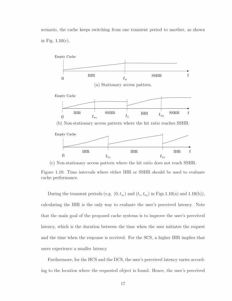
scenario, the cache keeps switching from one transient period to another, as shown
in Fig. 1.10(c).
t0 ts
Empty Cache
IHR SSHR
(a) Stationary access pattern.
t0 tv
Empty Cache
SSHRIHR
ts1
ts2
SSHRIHR
(b) Non-stationary access pattern where the hit ratio reaches SSHR.
t0
Empty Cache
IHR IHR
tv1tv2
IHR
(c) Non-stationary access pattern where the hit ratio does not reach SSHR.
Figure 1.10: Time intervals where either IHR or SSHR should be used to evaluatecache performance.
During the transient periods (e.g. (0, ts1) and (tv, ts2) in Figs 1.10(a) and 1.10(b)),
calculating the IHR is the only way to evaluate the user’s perceived latency. Note
that the main goal of the proposed cache systems is to improve the user’s perceived
latency, which is the duration between the time when the user initiates the request
and the time when the response is received. For the SCS, a higher IHR implies that
users experience a smaller latency.
Furthermore, for the HCS and the DCS, the user’s perceived latency varies accord-
ing to the location where the requested object is found. Hence, the user’s perceived
17

latency at a certain time can only be characterized by evaluating the average number
of links traversed to obtain the requested object at this time. This is called the in-
stantaneous average hit distance (IAHD). A lower IAHD implies that users experience
a smaller latency.
1.3 Motivations and List of Contributions
The proposed analytical model in this dissertation provides solutions for two fun-
damental problems: (1) estimating the instantaneous cache performance, assuming
fixed cache (FC) or temporary cache (TC); and (2) incorporating the TTL-based
consistency mechanism in the cache analysis.
Studies in [4,73,74,75,76] have shown that the access patterns obtained from real
traces exhibit strong variations due to many factors, such as a growing number of
objects, change in objects popularity, or a flash crowd8. Therefore, since the Web
user joins the network for a limited duration, the only way to calculate the hit ratio
experienced by the user is to estimate the IHR and the IAHD.
Moreover, estimating the IHR and the IAHD is crucial when the cache resources
are subject to change. For example, in the DCS with TCs, the total cache size
available for the cache system changes with time. Also, the TC is connected to the
network for a short period. Hence, it is important for this TC to reach a better hit
ratio quickly in order to enhance the hit ratio experienced by more users [12, 36, 71].
For example, in Fig. 1.10(a), the users who join the network while the TC is in the
8A large spike or surge in traffic to a particular Web site.
18

beginning of the transient state will experience low hit ratios. On the other hand,
users who join the network while the TC is closer to the steady state will experience
a better hit ratio.
However, the analytical models in the literature focused on evaluating the cache
performance in the steady state, assuming fixed cache resources, but did not provide
information about the cache performance during transient periods.
The proposed analysis considers NEM, TTL-IE, and TTL-T consistency mecha-
nism. TTL-T is the most widely used cache consistency mechanism on the Internet
today [28,35,37,39,77]. However, for simplification sake, the analytical models in the
literature considered either TTL-IE or NEM. More background regarding the related
analytical models in the literature will be discussed in Chapter 2.
Furthermore, based on the insights from the proposed analytical model, this dis-
sertation introduces a new replacement policy, named frequency-based-FIFO (FB-
FIFO), and a new sharing protocol, called promote cached objects (PCO), in order
to improve the user’s perceived latency. The performances of FB-FIFO and PCO
are evaluated under NEM, TTL-IE, and TTL-T, as will be discussed in detail in the
following chapters.
The main contributions of this dissertation are summarized in the following:
1- Introduction of a new analytical model for estimating the IHR of the SCS. The
cache may have an infinite size, or a finite size. For a finite-sized cache, FIFO and
LRU are considered. Also, the analysis considers two TTL implementations: TTL-IE
and TTL-T. This is discussed in Chapter 3.
2- Proposal of a new replacement policy called FB-FIFO. This is explored in
19

Chapter 39.
3- Introduction of a new analytical model for estimating the IHR and IAHD of
the HCS using LCE. LRU caching under TTL-IE or TTL-T is considered. Also, fixed
as well as temporary leaf caches are considered. This is analyzed in Chapter 4.
4- Proposal of a new sharing protocol for the HCS called PCO. This is examined
in Chapter 410.
5- Presentation of a new analytical model for estimating the IAHD for the DCS
with fixed or temporary caches. LRU caching under TTL-IE or TLT-T is considered.
This is discussed in Chapter 511.
1.4 Dissertation Roadmap
In this dissertation, the chapters are organized as follows. The background and related
work are discussed in Chapter 2. The analysis of the proposed SCS is presented in
Chapter 3. The analysis of the HCS and the DCS are introduced in Chapter 4 and
Chapter 5, respectively. Chapter 6 concludes the dissertation and discusses future
work. Finally, Appendix A and Appendix B include supplementary discussions for
Chapter 3 and Chapter 4, respectively.
9The work introduced in Chapter 3 under TTL-IE has been published in [12].10The work introduced in Chapter 4 for fixed leaf caches has been submitted to IEEE/ACM Trans.
Netw. on Dec 2012.11The simulation work for DCS with TCs, assuming the batch-arrival-batch-departure connectivity
model was published in [9, 10]. This work is not included in this dissertation for conciseness.
20

Chapter 2
Background
This chapter presents a brief background and discusses the related work for the con-
sidered cache systems. First, background for three main issues that affect the Web
cache performance are discussed: (1) HyperText Transfer Protocol (HTTP) and cache
consistency mechanisms are discussed in Section 2.1; (2) cache replacement policies
are discussed in Section 2.2; and (3) the access pattern characteristics are discussed
in Section 2.3. Then, Section 2.4 discusses the related analytical models in the litera-
ture for single cache systems. Sections 2.5 and 2.6 present the research on hierarchical
and distributed cache systems, respectively. The research on mobile cache systems is
discussed briefly in Section 2.7.
2.1 HTTP and Cache Consistency Mechanisms
The World Wide Web (Web) was invented by Tim Berners-Lee, a scientist at Eu-
ropean Council for Nuclear Research (CERN), in 1989. The Web was originally
developed to meet the demand for automatic information sharing between scientists
working in different universities and institutes all over the world. The basic idea of
the Web was to merge the technologies of personal computers, computer networking,
and hypertext into a powerful and easy to use global information system [78]. The
architecture of the Web uses the client-server model [79], where users access the Web
objects over the Internet from origin servers (OSs) using Web browser software (e.g.
21

Safari, Internet Explorer, Firefox, etc.).
Hypertext Transfer Protocol (HTTP) is an application layer protocol that relies
on the underlying TCP/IP protocols in order to provide reliable data transfer between
Web users and the OSs1. Moreover, the HTTP requests and responses are encoded
using headers to specify the interaction between the Web users, the OS, and the
intermediate Web cache [80].
Fig. 2.1(a) shows a set of request and response headers for a new object that is
not in cache (i.e. a cache miss). The location and the name of the requested object
are specified using uniform resource locator (URL). GET method is used to retrieve
a specific object indicated by the URL. Status Code 200 in the response indicates
that the object is retrieved successfully from the OS. The response includes 119494
bytes of data for the object. According to the Expires header, the object will expire
on (Mon, 25 Nov 2013 17:09:31 GMT). This means that the object life time (or the
time-to-live (TTL) value on Mon, 25 Nov 2012 17:09:31 GMT) is one year. If this
object is cached, the TTL value will decreases linearly with time until it reaches zero
(i.e. object expires) on (Mon, 25 Nov 2013 17:09:31 GMT). The cache can serve this
object without contacting the OS as long as the TTL value exceeds zero (i.e. as long
as the object is fresh).
The semantics of the GET method change to “conditional GET” if the request
message includes an If-Modified-Since header. For example, in Fig. 2.1(a), the Last-
Modified header indicates that the last time when the object has been modified is
1Web users may communicate with different types of servers (e.g. FTP). However, this disserta-tion is concerned with HTTP servers.
22

Request Headers
Request Method:GETRequest URL: http://s.ytimg.com/yts/swfbin/apiplayer-vflnKHczb.swf
Response Headers
Status Code:200 OKAccept-Ranges:bytes
Content-Length:119494Date:Sun, 25 Nov 2012 17:09:31 GMTExpires:Mon, 25 Nov 2013 17:09:31 GMTLast-Modified:Tue, 20 Nov 2012 19:52:07 GMT
(a) Cache miss.
Request Headers
Request Method:GETRequest URL: http://s.ytimg.com/yts/swfbin/apiplayer-vflnKHczb.swfIf-Modified-Since: Tue, 20 Nov 2012 19:52:07 GMT
Response Headers
Status Code:304 Not ModifiedDate:Mon, 26 Nov 2013 22:57:18 GMT
(b) Cache hit.
Figure 2.1: Sample HTTP request and response headers.
(Tue, 20 Nov 2012 19:52:07 GMT). Thus, the Last-Modified header can be used as
a cache validator. If this object is requested after it expires (i.e. after Mon, 25 Nov
2013 17:09:31 GMT), then the cache uses the If-Modified-Since request header to ask
the OS to send the object only if it was modified after (Tue, 20 Nov 2012 19:52:07
GMT). Otherwise, if the object was not modified (i.e. the cached object expired but
it is still valid), then the OS does not send the object to the cache. In this case, the
Status Code 304 in the response header indicates that the object is still valid and the
cache can serve this object (i.e. a cache hit), as shown in Fig. 2.1(b).
The cache consistency problem (i.e. keeping the cached objects valid) has drawn
attention as a key factor that affects the cache performance, especially for mobile
23

devices and wireless environments [36, 38, 81]. Cache consistency mechanisms are
mainly classified into strong consistency mechanisms and weak consistency mecha-
nisms. Strong consistency mechanisms, such as poll-each-read (PER) and call-back
(CB) ensure that the cache always serves valid objects, but they generate considerable
overhead traffic and increase the load on the OS [13, 38, 82, 83]. In PER, the cache
attempts to retrieve the object from the OS at each access and the OS only replies to
it with an acknowledgment when the cached object is valid. If the object is invalid,
the server sends the updated object to the cache. In CB, the OS sends an invalidation
message at each update to the caches that have invalid copies of the updated object.
In this case, the OS has to track the locations of cached objects.
In weak consistency mechanisms, the cache validates the cached object periodically
to reduce the overhead traffic with the OS and improve the user’s perceived latency.
However, weak consistency mechanisms might cause the cache to serve invalid objects.
Note that the cached copy of an object is valid if it is identical to the original copy
at the OS, which cannot be guaranteed without contacting the OS [35, 37, 84, 85].
Weak consistency mechanisms are particularly useful for Web applications in
which the user can tolerate (for a reasonable period of time) invalid objects. For
example, it is useful (or at least not harmful) to retrieve cached copies of online
newspapers, magazines, and personal home pages, even after their contents were up-
dated at the OS2. It has been shown that weak consistency is a viable and economical
approach to deliver content that does not have a strict freshness requirement [37].
2In any browser software, a user always has the option to validate the Web objects by pressingreload/refresh button.
24

Origin server
Cache
Time
Request
Cache miss
Object received
Request
Object is sent with
a new TTL value
Cache hit Object expires
TTL value
TTL-IE: object
is ejected
TTL-T: Object is
marked as expired
Time
Object expires
Request
Object is valid
Cache hit
Request
Cached object is invalid, fresh
copy is sent with a new TTL value
Object received
Object is modified
Cache missObject expires
Request
Object is sent with
a new TTL value
Cache miss
Object received
Object is
not cached
(a)
(b)
(c)
HTTP Get
request
HTTP Get
request
validation
request
(d)
(d) (d)(e) (e)
(f) (f) (g)
(h)
(i)
Figure 2.2: Object access under TTL-T and TTL-IE.
The concept of TTL [1] was introduced to support weak consistency as discussed
in Section 1.1.1. In this dissertation, two implementations for the TTL mechanism
are considered: TTL immediate ejection (TTL-IE) and typical TTL (TTL-T). The
example in Fig. 2.1 shows the SCS under TTL-T, where the cache has to validate
the expired object from the OS before serving it to the user. However, if the SCS
adopts TTL-IE, the object will be ejected once it expires on (Mon, 25 Nov 2013
17:09:31 GMT). Fig. 2.2 shows an example where an object is accessed from a cache
under TTL-T or TTL-IE. Note that, in TTL-T, if there is a high probability that the
expired cached objects will be updated in the next request, it might be useful to eject
the cached objects once they expire (i.e. use TTL-IE). This would not only avoid the
communication overhead caused by the validation requests, but also would prevent
25

the cache from being polluted by invalid objects.
2.2 Cache Replacement Policies
The cache size is limited compared to the huge number of Web objects3, and it is only
possible for a cache to store a fraction of the requested Web objects. Hence, cache
performance depends greatly on the replacement policy that is used to select which
objects to keep in cache in order to maximize the probability that future requests will
be satisfied from the cache. The replacement policy decides which object is ejected
from the cache to make room for a new object based on object characteristics, such as
popularity, recency (i.e. how recent the object is requested), size, or expiry rate. The
replacement policy may also account for network conditions, such as the bandwidth
available between the cache and the OS [12,13,14,15,86,87,88,89,90,91,92,93,94,95,
96, 97, 98, 99, 100, 101,102,103].
Some replacement policies consider only one object characteristic when making
replacement decisions. For example, Perfect-LFU uses the popularity of objects (i.e.
how many times the object has been requested) to decide which object to eject from
the cache. Another example is Largest File First (LFF), also called SIZE, which bases
the replacement decision on the size of the cached objects [89].
Furthermore, replacement policies may consider more than one object character-
istic. For example, LRFU [92], LFU-Dynamic Aging (LFU-DA) [94], and LRU-K [98]
consider both object popularity and recency. Another example is LRU-Threshold,
3There are 3.2 billion Web objects as suggested by Wolman et al. in 1999 [11].
26

which considers both recency and size [89]. Also, replacement policies may con-
sider both object characteristics and network conditions. For example, Greedy Dual
(GD) [97] considers the object recency and the number of hops between the cache
and the OS.
Several cache replacement policies were introduced to enhance the use of cache
storage. The following list is a brief description of replacement polices in the literature:
• Random (RAND): ejects a random object from the cache.
• First-In-First-Out (FIFO): ejects the oldest cached object.
• Least Frequently Used (LFU): ejects the object with the fewest references. There
are two versions of LFU:
1. Perfect-LFU: maintains the number of references for each object, even
if the object is not currently cached,
2. In-Cache-LFU: maintains the number of references for cached objects
only.
• Least Recently Used (LRU): ejects the least recently requested object.
• Largest File First (LFF): also called SIZE, ejects the largest object.
• LFU-Aging [15]: a variant of In-Cache-LFU, in which the request counts are
divided by 2 when the average value of all counters exceed a certain threshold.
• LFU* [96]: a variant of In-Cache-LFU, in which only the cached objects with
request count of one can be ejected from the cache. Hence, new requested objects do
not always added to the cache.
27

• LRU-Threshold: a variant of LRU, in which no object larger than the Threshold
is cached.
• LRU-k [98]: a variant of LRU, in which the cache maintain the last k request
times for each cached object. LRU-k ejects the object with the largest time elapsed
since the kth last request was made. LRU is a special case of LRU-k, where k=1.
• GreedyDual-Size (GDS) [95]: ejects the object with the smallest value for a
certain utility function that incorporates object size, recency, and the cost of retrieving
the object from the OS.
• Adaptive Replacement Cache (ARC) [91]: In ARC, the cache maintains two
LRU lists, with each has a length equals to the cache capacity4. The first list is
for one-time requested objects only. The second list is for objects that have been
requested more than once. A fraction of the objects on these two lists are physically
cached. The number of objects that are cached from the first list is determined by
a threshold, p. ARC ejects the least recently requested cached object from the first
list, if the number of cached objects that belong to the first list is greater than p.
Otherwise, ARC ejects the least recently requested cached object from the second
list.
2.3 Access Pattern Characteristics
The performance of the cache replacement policies depends greatly on the users’ ac-
cess pattern (or the workload). For example, LRU outperforms Perfect-LFU when
4The number of objects that can be cached simultaneously, assuming fixed object size.
28

the access pattern exhibits strong temporal locality5, due to correlation between re-
quests [6,93]. However, this is not true under the independent reference model (IRM),
where the object requests are independent and identically distributed.
Web access patterns have characteristics that were commonly used in developing
tractable analytical models for estimating the performance of Web caches. These
characteristics are summarized in the following list:
• The requests follow a Poisson process, where the inter-request times are inde-
pendent and exponentially distributed [96].
• Object popularity follows a Zipf-like distribution [6, 11, 104].
• The number of objects at Web servers is growing continuously [104].
• Object size distribution is heavy-tailed (Pareto) [96, 105]
• The expected lifetime (i.e. the initial TTL value) of an object is an exponential
random variable, as suggested in [11, 74].
• No correlation between the object lifetime and its popularity [79]
• Web traces exhibit strong temporal locality [106]. The relation between the
object popularity and the temporal locality is discussed below in the remainder of
this section.
There are two sources for the temporal locality: long-term and short-term popu-
larity. The long-term popularity is determined by the Zipf-like distribution, such that
the probability of the ith most popular object being selected from M objects is 1σiα
,
where σ =∑M
i=11iα
and α ∈ [0, 1] is the Zipf slope. This is true regardless of when
5The objects that are requested in the recent past are likely to be requested again in the nearfuture.
29

object i was last requested. This is called independent reference model (IRM), where
the identities of the requested objects are independent and identically distributed
(i.i.d.) random variables [107].
The short-term popularity (recency) occurs due to the temporal correlation be-
tween object requests. This is called a Markov reference model (MRM), where the
probability of selecting an object i depends on when this object was requested in the
near past [108].
The study in [6] showed that the temporal locality created due to the long-term
popularity is similar to that observed in real traces. Thus, it is not necessary (at
least for obtaining accurate qualitative results) to model the temporal correlations.
A more careful study of real traces revealed that the long-term popularity alone does
not suffice to fully capture the temporal locality exhibited by real traces [93].
The studies in [63, 109] showed that the performance of a large cache does not
depend on the correlation in the request traffic. Particularly, the studies in [63, 109]
showed that the LRU cache performance is asymptotically identical to the case of
IRM, if the cache is large. Furthermore, Jelenkovic et al. [62] determined the smallest
cache size beyond which this asymptotic insensitivity property holds.
2.4 SCS Analytical Models in the Literature
This section presents the related analytical models for the SCS proposed in Sec-
tion 1.1.1. IRM with fixed-size objects was widely used to develop tractable analyt-
ical caching models, especially when a cache with finite size was considered. In this
30

section, all the presented analytical models use this assumption.
Wolman et al. [11] proposed an analytical model for estimating the steady state hit
ratio (SSHR) for a single cache with infinite capacity (Infinite Cache). The analysis
in [11] considered object lifetime, which is exponentially distributed and correlated
with the object popularity. The study in [11] showed that the SSHR is very sensitive
to the object expiry rate. The results in [11] also showed that the increase in the
request rate, relative to the expiry rate, enhances the SSHR.
Breslau et al. [6] proposed an analytical model for estimating the SSHR of Infinite
Cache and Perfect-LFU, assuming objects that do not expire. The results in [6]
showed that the SSHR of Perfect-LFU increases logarithmically or as a small power
as a function of cache size.
Analytical models for estimating SSHR of LRU and FIFO were also introduced
in [8, 61, 62, 63, 64, 65, 66].
Gelenbe et al. [66] extended the analysis provided for FIFO in [99] in order to
show that FIFO and RAND replacement policies reach the same SSHR. Dan et al. [65]
developed approximate analytical models for estimating the SSHR of LRU and FIFO.
The study in [65] showed that LRU always outperforms FIFO in steady state.
Jelenkovic et al. [64] showed that computing the LRU miss probability is the same
as computing the move-to-front (MTF) search cost distribution. Also, the study
in [61] proposed an analytical model for estimating the approximate SSHR of a single
cache running LRU.
The analytical models introduced in [61,62,63,64,65,66], however, assumed objects
that do not expire. More realistic studies in [8, 38] provided an analytical model for
31

LRU cache under strong cache consistency model, where the cache has to ensure that
the cached object is identical to the one at OS whenever the object is requested (i.e.
poll-each-read (PER)). Also, Krishnamurthy et al. [110] studied the single LRU cache
under TTL-T using trace-driven simulations.
While the analytical models in previous studies focused on estimating the SSHR,
assuming stationary access pattern, to the best of my knowledge, the work in this
dissertation is the first attempt to develop an analytical model to study the evolution
of LRU and FIFO with time under TTL-based consistency.
2.5 Research on Hierarchical Cache Systems
Hierarchical Caching was first proposed in the Harvest project to share the interests of
a large community of users, and has already been implemented in several countries [7,
111,112,113]. With hierarchical caching, caches are placed at different network levels.
At the bottom level of the hierarchy are users’ caches. When a request is not satisfied
by a user’s cache, the request is sent to the institutional cache. If the object is not
in the institutional cache, the request travels to the regional cache, which in turn
forwards unsatisfied requests to the national cache. If the object is not found at any
cache level, the national cache directly contacts the OS. The main drawback of this
scheme is that every hierarchy introduces additional delays. Moreover, higher level
caches could get overwhelmed with requests from caches at lower levels, which causes
higher level caches to introduce more delays [3, 7, 114, 115,116,117,118].
As discussed in Section 1.1.2, cooperation between caches at different network
32
levels requires a sharing protocol. Section 2.5.1 presents the main sharing protocols
proposed in the literature. Then, the HCS analytical models in the literature are
discussed in Section 2.5.2.
2.5.1 HCS Sharing Protocols
Many sharing protocols were proposed in the literature to allow the cooperation
between caches at different levels of the cache hierarchy. Leave copy everywhere
(LCE) was developed in the Harvest project [112]. In LCE, when the object is found,
either at a cache or at the OS, it travels down the hierarchy, and a copy is left at each
of the intermediate caches. The main drawback of LCE is that it allows objects that
are effectively one-timers6 to pollute the cache hierarchy. Moreover, LCE requires
large caches at the high levels of the hierarchy (i.e. caches that are close to the OS)
and these caches may become bottlenecks between the users and the OS [25, 26].
The studies in [24, 25, 26, 119] developed sharing protocols that achieve higher
steady state average hit distance (SSAHD) than LCE under the assumption that the
objects do not expire. Che et al. [25] introduced two design principles to enhance the
LCE performance in a two-level LRU cache hierarchy. First, the root cache size has
to be larger than the leaf cache size. Second, objects that are effectively one-timers
should not be cached at all throughout the cache hierarchy.
Based on these principles, Che et al. [25] introduced a sharing protocol wherein
a cache is allowed to store an object if the object is not effectively a one-timer with
6A one-timer is an object that is requested once, and will never be requested again. The objectis effectively a one-timer if its request rate is too low to generate a cache hit [25].
33

respect to this cache. Hence, the small leaf cache is preserved for the most popular
objects (objects with high request rate, such that they generate cache hits for a small
LRU cache), while the larger root cache may store objects with lower popularity. The
objects that are effectively one-timers (with respect to the root cache) are not cached
in any cache throughout the cache hierarchy. Also, to account for the situation when
the object popularity decreases, if a cached object is ejected from the leaf cache, it
will be sent to the root cache if the root cache does not have this object. The main
problem in this protocol is that it requires the leaf cache to constantly track the access
frequency of recently requested objects. Also, the average maximum object access
interval without a cache miss has to be measured periodically for every cache in the
cache hierarchy. This allows each cache to decide whether an object, with a certain
request rate, is effectively one-timer or not.
Wong et al. [119] have proposed a sharing protocol for LRU cache hierarchy,
called DEMOTE, where the leaf cache sends the ejected objects to the root cache.
Additionally, when the root cache forwards an object to the leaf cache, it moves its
local copy to the tail of its LRU list (to be ejected in the next replacement). The
goal of DEMOTE is to avoid the duplication of the same objects at multiple levels.
Laoutaris et al. [24] introduced two sharing protocols: leave copy down (LCD)
and move copy down (MCD). In LCD, when the object is found, it travels down the
hierarchy and a copy is left only at the cache that is just below the level where the
object is found. In MCD, when the object is found, it moves down the hierarchy to
the cache that is just below the level where the object is found. Laoutaris et al. [24]
showed by simulations that LCD outperforms LCE, DEMOTE, and MCD in terms of
34

SSAHD that the LRU cache hierarchy can achieve without the considerable overhead
of the sharing protocol proposed by Che et al. [25].
In this dissertation, the design and analysis of a new sharing protocol, called
PCO, is introduced. PCO achieves higher SSAHD than LCE and LCD. Also, like
LCD, PCO is less complex than the sharing protocol proposed in [25], as will be
discussed in detail in Chapter 4.
2.5.2 HCS Analytical Models in the Literature
Analytical models for estimating the steady state hit ratio (SSHR) for LCE under
TTL-IE were introduced in [7, 37, 120]. A cache hierarchy based on a tree topology
was analyzed in [7, 37], while Tang et al. [120] introduced an analytical model for
unstructured P2P networks. These models assumed infinite sized caches. Thus, they
generate an optimistic cache performance, since caches are limited in size compared
to the huge number of Web objects [11].
The studies in [25, 41] introduced analytical models for an LRU cache hierarchy.
The study by Che et al. [25] is the closest one to the proposed HCS analysis in
Chapter 4. Che et al. used the mean field approximation approach for estimating
the SSHR of a two-level cache hierarchy using LCE. Che et al. assumed that LRU
runs locally at each cache and all the objects have the same size. These are the same
assumptions adopted by the proposed analysis in Chapter 4. Moreover, Laoutaris
et al. [41] introduced an analytical model for a two-level cache hierarchy using LCD
based on the approximations proposed by Che et al. [25].
Compared to the proposed analysis in Chapter 4, the analytical models in [25]
35

and [41] have two drawbacks. First, they do not account for object expiry. Second,
analytical models in [25] and [41] do not capture the transient behavior of the cache
hierarchy under a non-stationary access pattern, as discussed in Section 1.3.
To the best of my knowledge, this dissertation introduces the first analytical model
that characterizes the transient performance of an LRU cache hierarchy under TTL-
IE or TTL-T. Moreover, this dissertation proposes the first analytical model that
considers an LRU cache hierarchy with temporary leaf caches (TLCs), as discussed
in Section 1.1.4.
2.6 Research on Distributed Caching Systems
In distributed caching, no intermediate caches are set up, and there is only one level
of caches (e.g. users’ caches, or institutional caches) that cooperate to serve each
others’ misses. Distributed caching offers some different advantages than hierarchical
caching, including a lower access latency, a higher degree of fault tolerance, and a
more uniform load distribution [3, 7, 121, 122,123,124,125,126,127].
Plenty of sharing protocols were proposed in the literature to allow the cooperation
between sibling caches in a DCS, as discussed in Section 1.1.3. In Section 2.6.1, the
main DCS sharing protocols are described. Then, Section 2.6.2 presents the DCS
analytical models in the literature.
2.6.1 DCS Sharing Protocols
Internet caching protocol (ICP) was designed for the NLANR project [7, 44, 111]. In
ICP, the sibling cache cannot resolve another cache request, if the sibling cache does
36

not have the requested object. Only cache hits are resolved by the nearest sibling
cache [29, 128]. In ICP, the cache distinguishes between the local requests and the
remote requests, and the caches in the DCS do not coordinate their replacement poli-
cies, as discussed in Section 1.1.3. Note that ICP does not improve the performance
of individual caches. On the other hand, the users experience better performance due
to remote cache hits. This requires multicasting the queries, and result in ICP gen-
erating considerable traffic on every cache miss. Also, ICP results in long connection
time to find a remote cache with the requested object [7].
Cache Summary, developed by Fan et al. [44], and Cache Digest, developed by
Rousskov et al. [129], avoid the drawbacks of ICP by allowing caches in a DCS to
periodically exchange information about their contents. Moreover, to achieve more
efficient and scalable DCS, these protocols may utilize a hierarchical infrastructure
for storing meta-data about the locations of objects in the DCS [7]. Note that the
hierarchical infrastructure is used only for distributing the locations of cached objects
in the DCS, rather than caching the objects themselves. Also, note that ICP, Cache
Summary, and Cache Digest protocols allow multiple copies of the same objects to
be stored at different locations within the DCS.
Cache array routing protocol (CARP) was introduced by Valloppillil et al. [45],
where at most one copy of an object can be stored in the DCS at a time7. In CARP,
the URL-space is divided among the caches in the DCS. Thus, the request for the
same URL is always forwarded to the same cache. In CARP, a local cache does not
store the object that is served from the remote cache in the DCS. Also, like ICP,
7This is also called hash-based caching, single copy caching, or one-copy heuristic (1CH).
37
the replacement policy is also applied on individual caches independently. However,
when an object is requested, the remote cache may increase the caching priority for
this object [44, 130, 131].
Global Cache [44] is another approach that prevents the redundant caching of
the same object. Global Cache is a hypothetical approach, where it is assumed that
the caches in the DCS coordinate their replacement policy and appear as one unified
cache, with a cache size that is equal to the aggregate cache sizes in the DCS. In
this case, if the local cache is full and it needs to store more objects, it may use the
available cache capacity on another cache in the DCS. If all caches in the DCS are
full, then the replacement policy is applied across all caches in DCS to decide which
objects to eject. In this case, at most one copy of an object may exist in the DSC.
Hence, the analysis for the SCS introduced in Chapter 3 can be used for estimating
the IHR of the DCS using Global Cache.
In Chapter 5, the proposed DCS using ICP under TTL-based consistency is evalu-
ated. I believe that the proposed analysis of ICP can be extended to CARP. However,
this will be considered in future work.
2.6.2 DCS Analytical Models in the Literature
Analytical models for estimating the steady state hit ratio (SSHR) of the DCS under
TTL-IE were introduced in [7]. In [7], it is assumed that the caches exchange their
meta-data about their contents instantaneously. It is also assumed that the caches
have infinite size.
Moreover, the study in [40] introduced an analytical model for estimating the
38

SSHR of the DCS in the context of LRU. The model proposed in [40] is based on
the analysis proposed by Dan et al. [65]. The study in [40] also considered a DCS
with dependent-LRU, where the local LRU list is updated because of remote hits.
However, the study in [40] assumed objects that do not expire.
To the best of my knowledge, the work in this dissertation is the first attempt to
introduce analysis for estimating the IHR and the IAHD of the DCS running LRU
under TTL-based consistency. This will be discussed in Chapter 5. Also, possible
extension of the proposed analysis for a DCS with dependent-LRU will be discussed
briefly in Chapter 6.
2.7 Research on Mobile Cache Systems
In Mobile Ad-Hoc Networks (MANETs), cooperative caching on mobile devices is
essential to reduce the usage of limited bandwidth, save battery life, and improve
the user’s perceived latency [9, 10, 13, 48, 49, 122, 132, 133]. Furthermore, caching on
vehicles is promising since they can provide more processing power and enough space
to accommodate a cache with large storage size, unlike traditional mobile devices (e.g.
smart phones) [36, 50, 134]. On the other hand, cooperative caching schemes must
account for disconnections of mobile devices, due to mobility, as well as the limited
battery life of mobile devices [9].
Cooperative caching in MANET was considered in many studies [35, 71, 135, 136,
137,138,139,140,141,142], as will be discussed briefly in the remainder of this section.
However, to the best of my knowledge, the work in this dissertation is the first attempt
39

for estimating the performance of cooperative caching on mobile devices that run LRU
under TTL-based consistency.
The study in [135] introduced three cooperative caching systems: CacheData,
CachePath, and HybridCache. In CacheData, the node (mobile user) caches the
passing-by popular objects locally in order to serve future requests. In CachePath,
intermediate nodes between the requesting node and the origin server (OS) store the
location (path information) where the object is cached (i.e. the location of the request-
ing node). Later, when this object is requested from one of those intermediate nodes,
the request will be redirected to that location, rather than the OS, which reduces the
response delay. Note that multiple copies of the same object or object path might be
cached in the MANET, since each node makes the cache decision independently. The
simulation results in [135] showed that CachePath outperforms CacheData when the
cache size is small or the object expiry rate is low, while CacheData performs better
in other situations. Hence, HybridCache was introduced in [135] to take advantage
of both CacheData and CachePath. Particularly, when a node forwards an object, it
may cache the object or path based on some criteria, such as object size and object
expiry rate.
The main disadvantage of the systems introduced in [135] is that the cached object
(or path information) will only be accessed if it is in the path of the request to the OS.
Hence, the cache hit ratio depends greatly on the node positions relative to each other
and relative to the access point. The system introduced by Lim et al. [136] overcomes
this problem. In [136], the node broadcasts the request to all other nodes in the
network, then the requesting node retrieves the object from the first acknowledging
40

node (which has the required object) it hears from. Although this approach suffers
from high bandwidth usage due to the broadcasts, it is simple and achieves a low
latency.
Artail et al. [71], proposed a cooperative and adaptive caching system (COACS)
for MANETs. COACS consists of three types of nodes (mobile users): caching nodes
that cache previously requested objects, query directories that index the cached ob-
jects by holding the queries along with the locations of the corresponding caching
nodes (i.e. store the path information like CachePath), and requesting nodes (any
node, including a query directory or a caching node). In COACS [71], when a node
requests an object that is not cached by any caching node in the system, the OS is
accessed to retrieve this object. Upon receiving the object, the node that requested
the object will act as a caching node by caching this object. The nearest query di-
rectory to the caching node will cache the query and make an entry in its hash table
to link the query to its response.
Like the approach in [136], all the caching nodes in COACS have to be checked
for the requested object before sending the request to the OS. However, instead of
broadcasting the request, the request in COACS is forwarded from a query directory
to another until the object is found or until all the query directories are checked.
Hence, COACS reduces the bandwidth usage due to the broadcasts used in [136].
The simulation results in [71] showed that COACS outperforms both CacheData
and CachePath. Furthermore, the study in [71] provides analysis for estimating the
upper and lower limits of average response delay, by setting the average hit ratio to one
and zero, respectively. However, they did not provide any expression for calculating
41
the average hit ratio. Also, the proposed work in [71] did not consider the cache
consistency problem. Later in [35], a cache consistency mechanism that is built on
top of COACS has been proposed.
In the proposed cooperative caching system in this dissertation, two types of
nodes (mobile users) are assumed: caching nodes (mobile device hosting caches)
and requesting nodes (any node in the MANET including the caching nodes). Like
COACS [71], all the caching nodes in the MANET have to be checked for the requested
object before sending the request to the OS. However, the proposed system does not
need query directories. Note that, in the proposed HCS, the MANET contains only
one caching node (i.e. the temporary leaf cache (TLC)), while in the proposed DCS,
the requesting node may only query the nearest caching node in the MANET (i.e. the
local TC). Also, similar to the approach proposed in [136], the local TC broadcasts
the request to the other caching nodes in the MANET (i.e. remote TCs), if it does
not have the requested objects.
Note that the work in this dissertation is not concerned with evaluating the
MANET routing protocols that are used to determine the multihop communication
path, between the mobile user and the location of the requested object, that mini-
mizes the energy consumption and the response delay [143,144,145]. In the proposed
HCS the mobile user communicates only with its TLC, which has a direct link to the
access point. Also, in the DCS, it is assumed that any mobile user communicates
only with its local TC, which has a direct link to the access point, or to any remote
TC within the MANET, as will be discussed in detail in Section 5.2.
42

Chapter 3
Analysis of the Single Cache System (SCS)
This chapter introduces a novel analytical model for characterizing the hit ratio of
a single cache system (SCS) as a function of time, as discussed in Section 1.2. The
considered single cache can be thought of as a Web cache that is installed at the ISP,
or at the main router of an institution (e.g. university, company, etc.) as shown in
Fig 1.1. Also, it might be a local cache installed at a Web user (e.g. browser cache).
The proposed analysis considers two implementations for TTL consistency: typical
TTL (TTL-T) and TTL immediate ejection (TTL-IE). As discussed in Section 1.1.1,
the analysis also considers the case where objects do not expire, which is called non-
expiry model (NEM).
The proposed analysis models the activity of a single cache with infinite capacity
(Infinite Cache) or finite capacity. The cache capacity is defined as the number
of objects that can be stored in a cache simultaneously, assuming that all objects
have the same size. For finite cache capacity, the proposed analysis considers two
replacement policies: FIFO and LRU. Also, steady state analysis of Perfect-LFU
is discussed. Note that the proposed analysis in this chapter can be extended for
cooperative cache systems (e.g. hierarchical caching), as will be discussed in the
subsequent chapters in this dissertation.
Moreover, this chapter introduces a new replacement policy, called frequency-
based-FIFO (FB-FIFO). FB-FIFO improves the instantaneous hit ratio (IHR) by
43

creating a variable-sized protected cache segment for objects that are not effectively
one-timers, as will be discussed in detail in this chapter. Note that no analysis is
provided for FB-FIFO.
The remainder of this chapter is organized as follows. First, the analysis assump-
tions are discussed in Section 3.1. Second, assuming a stationary access pattern, the
proposed analysis for Infinite Cache, Perfect-LFU, FIFO, and LRU is presented in
Sections 3.2, 3.3, 3.4, and 3.5, respectively. Third, the proposed analysis is general-
ized for a non-stationary access pattern in Section 3.6. Next, FB-FIFO is presented
in Section 3.7. Section 3.8 is an evaluation for the IHR of a single cache under NEM
and TTL-IE, while Section 3.9 is a steady state evaluation for a single cache under
TTL-IE and TTL-T. Finally, Section 3.10 summarizes the findings of this section.
3.1 Analysis Assumptions
The proposed analysis assumes that the origin server (OS) has M(t) objects at time
t. Allowing the number of OS objects to change with time allows the analysis to
accommodate the continuous generation of new popular objects [12, 74, 75].
Consider the interval (0, tv) or (tv,∞) in Fig. 1.10(b) where the number of objects
is fixed, such that M(t) ≃ M . Users request those M objects according to a Poisson
process with rate β [146]. The probability of each request being for one of the M
objects is determined by a Zipf-like distribution [6, 11]. In this distribution, the
probability of the ith most popular object being selected is 1/(σiα), where σ =
∑Mi=1 1/iα and α is the Zipf slope such that 0 < α ≤ 1. Note that the probability of
44

requesting an object i is independent of past history (i.e. the independent reference
model (IRM) is assumed) [93, 99, 108].
The overall Poisson request process can be modeled as a sum of M independent
Poisson processes, with each representing the requests for one of the M objects [146].
The average request rate of the Poisson process for object i ∈ [1, M ] at time t, is
λ(i) =β
σiα
The proposed analysis assumes that the initial TTL value of a cached object,
i, is exponentially distributed with mean 1/µ(i) that is independent from object
popularity, as suggested in [11, 13, 35, 74].
It is assumed that α, β, and µ(i) are not a function of time. However, the proposed
analysis can be extended to cover these cases, which are excluded from this chapter
merely for conciseness1.
In this chapter, the cache capacity, C, is defined as the number of objects that
can be cached simultaneously (i.e. C is the cache size divided by the object size). For
simplicity, it is assumed that the cache can store up to C objects, where the objects
are of the same size.
Note that assuming the IRM with fixed-size objects is widely used to develop
tractable analytical cache models, especially when the cache has finite size [13, 24,
25,35,38]. However, these assumptions might not accurately model empirical traces.
Thus, an interesting extension of the proposed model would be to incorporate tem-
1In Chapter 4, the case where the request rate at the cache is a function of time will be considered.
45

poral correlations, as well as assuming objects with different sizes.
In the following sections, continuous time Markov chain analysis [147] is used to
calculate the IHR for M objects, H(t). Since the Poisson request processes for each
of the M objects are independent, it is possible to start by analyzing the probability
that the request for object i at time t is not served by the cache, S(t, i). Then, H(t)
will be calculated as
H(t) =M
∑
i=1
1 − S(t, i)
σiα(3.1)
Assuming a stationary access pattern, analytical solutions for Infinite Cache,
Perfect-LFU, FIFO, and LRU are developed in Section 3.2, Section 3.3, Section 3.4,
and Section 3.5, respectively. Then, the analysis is extended for a non-stationary
access pattern in Section 3.6.
3.2 Analysis of Infinite Cache
This section presents the analysis of a single Infinite Cache assuming a stationary
access pattern, as shown in Fig. 1.10(a). First, the analysis for non-expiry model
(NEM) is discussed in Section 3.2.1. Second, the analysis for TTL immediate ejection
(TTL-IE) is discussed in Section 3.2.2. Third, the analysis for typical TTL (TTL-T)
is discussed in Section 3.2.3.
Note that estimating the steady state hit ratio (SSHR) of Infinite Cache has
been done under TTL-IE in [11], and the contribution of this section is providing an
analytical model for estimating the IHR, as well as considering TTL-T.
46

State
0
State
1
λ(i)
Figure 3.1: Infinite Cache Markov chain for object i under NEM.
3.2.1 Infinite Cache under NEM
In NEM, the objects do not expire, and thus, cached objects are always fresh. Hence,
the Infinite Cache does not eject an object once it is cached. The state of the cache
for an object i can be modeled using a Markov chain, as shown in Fig. 3.1. In Fig. 3.1,
there are two states:
• Non-cache state (NCS): state 0, which corresponds to when object i is not in
the cache.
• Cache-fresh state (CFS) : state 1, which corresponds to when object i is in the
cache.
In Fig. 3.1, the rate at which the object moves from state 0 to state 1 is equal to
the object request rate (i.e. λ(i)), and the process does not return to state 0. Thus,
the Markov chain flow matrix of object i, Q(i), is given by
Q(i) =
−λ(i) λ(i)
0 0
Assuming an empty cache at time t = 0, the probability matrix of object i at time
47

t, P(t, i), is calculated using (3.2) [146, 147].
P(t, i) = exp(Q(i) t) (3.2)
The probability that a request for object i at time t will not be served from the
cache, S(t, i), is equal to the probability that object i is in state 0 at time t, P (t, i, 0).
Hence, S(t, i), is calculated using (3.3) [146].
S(t, i) = P (t, i, 0) = [P(t, i)]1,1 = e−λ(i)t (3.3)
where the notation [.]r,c denotes the element in row r and column c of a matrix [146].
The IHR is then calculated using (3.1). Note that, assuming a stationary access
pattern, limt→∞ S(t, i) = 0, and the SSHR is
limt→∞
H(t) =
M∑
i=1
λ(i)
β= 1 (3.4)
3.2.2 Infinite Cache under TTL-IE
In TTL-IE, objects are merely ejected when they expire. The state of the cache with
respect to an object i can be modeled using a Markov chain, as shown in Fig. 3.2.
Like Fig. 3.1, the Markov chain in Fig. 3.2 has two states:
• State 0 (NCS): corresponds to when object i is not in the cache.
• State 1 (CFS) : corresponds to when object i is in the cache.
In Fig. 3.2, the rate at which the object moves from state 0 to state 1 is equal to
the object request rate (i.e. λ(i)) and the rate at which the process returns to state
48

State
0
State
1
λ(i)
µ(i)
Figure 3.2: Infinite Cache Markov chain for object i under TTL-IE.
0 is equal to the object expiry rate (i.e. µ(i)). Hence, the Markov chain flow matrix
of object i, Q(i), is given by
Q(i) =
−λ(i) λ(i)
µ(i) −µ(i)
Assuming an empty cache at time t = 0, the probability matrix of object i at time
t, P(t, i), is calculated using (3.2). Then, S(t, i) is calculated as
S(t, i) = P (t, i, 0) = [P(t, i)]1,1 (3.5)
where [P(t, i)]1,1 is calculated using (3.6) [146].
[P(t, i)]1,1 =µ(i)
λ(i) + µ(i)+
λ(i)
λ(i) + µ(i)e−(λ(i)+µ(i))t (3.6)
The IHR is then calculated using (3.1). Also, limt→∞ S(t, i) can be calculated as
limt→∞
S(t, i) =µ(i)
λ(i) + µ(i)(3.7)
Hence, the SSHR is
49

State
0
State
1
State
2
λ(i)
µ(i)ς(i)
Figure 3.3: Infinite Cache Markov chain for object i under TTL-T.
limt→∞
H(t) =
M∑
i=1
λ(i)
β
(
λ(i)
λ(i) + µ(i)
)
(3.8)
3.2.3 Infinite Cache under TTL-T
In TTL-T, unlike TTL-IE, the object is not ejected from the cache when it expires.
The cache just marks this object as “expired”. Compared to TTL-IE, the Markov
chain under TTL-T has an extra state that is added to accommodate object i when
it expires, as shown in Fig. 3.3. The Markov chain in Fig. 3.3 has three states:
• Non-cache state (NCS): state 0, corresponds to when object i is not in the cache.
• Cache-fresh state (CFS): state 1, corresponds to when object i is in the cache
and is fresh.
• Cache-expired state (CES): state 2 , corresponds to when object i is in the cache
and is expired.
In Fig. 3.3, the rate at which the object moves from state 0 to state 1 is equal to
the object request rate (i.e. λ(i)), and the process does not return to state 0. When
an object expires, it moves from state 1 to state 2 with a rate that is equal to the
object expiry rate (i.e. µ(i)). The object returns from the current CES to the CFS,
50
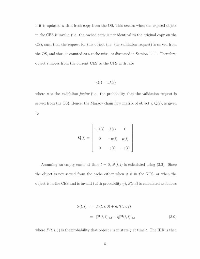
if it is updated with a fresh copy from the OS. This occurs when the expired object
in the CES is invalid (i.e. the cached copy is not identical to the original copy on the
OS), such that the request for this object (i.e. the validation request) is served from
the OS, and thus, is counted as a cache miss, as discussed in Section 1.1.1. Therefore,
object i moves from the current CES to the CFS with rate
ς(i) = ηλ(i)
where η is the validation factor (i.e. the probability that the validation request is
served from the OS). Hence, the Markov chain flow matrix of object i, Q(i), is given
by
Q(i) =
−λ(i) λ(i) 0
0 −µ(i) µ(i)
0 ς(i) −ς(i)
Assuming an empty cache at time t = 0, P(t, i) is calculated using (3.2). Since
the object is not served from the cache either when it is in the NCS, or when the
object is in the CES and is invalid (with probability η), S(t, i) is calculated as follows
S(t, i) = P (t, i, 0) + ηP (t, i, 2)
= [P(t, i)]1,1 + η[P(t, i)]1,3 (3.9)
where P (t, i, j) is the probability that object i is in state j at time t. The IHR is then
51

calculated using (3.1). Note that, under TTL-T, limt→∞ S(t, i) can be calculated as
limt→∞
S(t, i) =ηµ(i)
ς(i) + µ(i)(3.10)
where limt→∞[P(t, i)]1,1 = 0 and limt→∞[P(t, i)]1,3 = µ(i)/(ς(i) + µ(i)). Hence, the
SSHR of Infinite Cache under TTL-T is calculated as
limt→∞
H(t) =M
∑
i=1
λ(i)
β(1 −
ηµ(i)
ς(i) + µ(i)) (3.11)
Also, note that the average validation request rate can be calculated as
ν(t) =M
∑
i=1
λ(i)P (t, i, 2)
3.3 Analysis of Perfect-LFU
This section discusses how the analysis of Infinite Cache, introduced in Section 3.2,
can be modified to estimate the SSHR of a single Perfect-LFU cache. No analysis is
provided for estimating the IHR for Perfect-LFU.
The SSHR is estimated for a single Perfect-LFU cache under NEM, TTL-IE,
and TTL-T by replacing the number of objects, M , with the cache capacity, C,
in (3.4), (3.8), and (3.11), respectively2. Hence, the SSHR of a single Perfect-LFU
cache under NEM, TTL-IE, and TTL-T is calculated using (3.12), (3.13), and (3.14),
2This idea is used in [6] for estimating the SSHR of Perfect-LFU under NEM.
52

respectively. Note that the objects in [1, C] are the most popular objects.
limt→∞
H(t) =
C∑
i=1
λ(i)
β(3.12)
limt→∞
H(t) =C
∑
i=1
λ(i)
β
(
λ(i)
λ(i) + µ(i)
)
(3.13)
limt→∞
H(t) =
C∑
i=1
λ(i)
β(1 −
ηµ(i)
ς(i) + µ(i)) (3.14)
Note that, like Infinite Cache, limt→∞ S(t, i) for Perfect-LFU under TTL-IE and
TTL-T is calculated using (3.7) and (3.10), respectively.
Also, for Perfect-LFU under TTL-T, the average validation request rate is calcu-
lated as follows
limt→∞
ν(t) =
C∑
i=1
λ(i) limt→∞
P (t, i, 2)
=C
∑
i=1
λ(i)µ(i)
ς(i) + µ(i)
3.4 Analysis of FIFO
In this section, a new analytical model for a single FIFO cache is presented. The
proposed analysis assumes a stationary access pattern, as shown in Fig. 1.10(a). First,
the analysis for NEM is discussed in Section 3.4.1. Then, the analysis for TTL-IE
and TTL-T is discussed in Sections 3.4.2 and 3.4.3, respectively.
53

State
0
State
1
State
2
State
State
C
C − 1
λ(i)
ǫz(t, i) ǫ
z(t, i) ǫz(t, i) ǫ
z(t, i)
ǫz(t, i)
Figure 3.4: FIFO Markov chain for object i under NEM.
3.4.1 FIFO Cache under NEM
In FIFO, when a new object is requested, the oldest cached object is ejected, if the
cache is full. The state of the cache with respect to an object i can be modeled using
the Markov chain shown in Fig. 3.4. Similar to the analysis in Section 3.2.1, the
Markov chain in Fig. 3.4 has two types of states:
• Non-cache state (NCS): state 0, corresponds to when object i is not in the cache.
• Cache-fresh states (CFSs): states 1 to C, correspond to when object i is in the
cache.
The CFSs represent the relative time at which object i was brought into the
cache. State C corresponds to the most recently cached object. The recency of a
cached object decreases as the object goes from CFS j to the CFS j − 1. The CFS
j = 1 corresponds to the oldest object in the cache.
In Fig. 3.4, an object i moves from the NCS to state C with rate λ(i) (i.e. when
the object is requested, but not currently cached). Furthermore, an object i moves
from the current state to the next lower-numbered one whenever a new object is
introduced into the FIFO cache. Thus, the rate at which a cached object i moves
from the current CFS to the previous state, ǫ(t, i), can be calculated as
54

ǫ(t, i) =M
∑
m=1,m6=i
λ(m)P (t, m, 0) (3.15)
where P (t, i, j) is the probability that object i is in state j at time t. The flow matrix
for the Markov chain in Fig. 3.4 is
Q(t, i) =
−λ(i) 0 . . . 0 0 λ(i)
ǫ(t, i) −ǫ(t, i) . . . 0 0 0
......
......
......
0 0 . . . ǫ(t, i) −ǫ(t, i) 0
0 0 . . . 0 ǫ(t, i) −ǫ(t, i)
(3.16)
Assuming an empty cache at time t = 0, P(t, i) is then calculated using (3.2),
and S(t, i) is calculated using (3.5) (i.e. S(t, i) = P (t, i, 0)). Then, the IHR, H(t), is
calculated using (3.1).
However, from (3.15) and (3.5), H(t) cannot be calculated without having the
probabilities P (t, i, 0), ∀i ∈ [1, M ], which are initially unknown. To overcome this
problem, the following analysis is proposed based on the contraction mapping the-
ory [32, 33, 34].
The proposed analysis starts by initializing P 0(t, i, 0), ∀i ∈ [1, M ] to 1. Thus,
P 0(t, i, j)|j>0 is initialized to 0, such that∑C
j=0 P 0(t, i, j) = 1. Thus, (3.15) is rewrit-
ten for the first iteration of the proposed analysis, z = 1, as
55

Table 3.1: Iterative analysis for estimating the IHR of a single FIFO cache underNEM.
1- Set: P 0(t, i, 0) = 1, ∀ i ∈ [1, M ]2- Set: z = 03- Do4- z = z + 15- Calculate: ǫz(t, i), ∀ i ∈ [1, M ] using (3.18)6- Calculate: Pz(t, i), ∀ i ∈ [1, M ] using (3.19)7- Calculate: Sz(t, i), ∀ i ∈ [1, M ] using (3.20)8- Calculate: Hz(t) using (3.21)9- While (Hz(t) 6= Hz−1(t))10- Output H(t) = H∗(t) = Hz(t)
ǫ1(t, i) =M
∑
m=1,m6=i
λ(m) (3.17)
where the superscript denotes the iteration at which the variable is calculated. Then,
the flow matrix at z = 1, Q1(t, i), is established using ǫ1(t, i) according to (3.16).
Then, the probability matrix P1(t, i) is calculated using (3.2). Afterwards, S1(t, i)
is calculated using (3.5), and H1(t) is calculated using (3.1). This procedure is re-
peated, and the analysis approaches the exact solution for the IHR iteratively and
terminates after reaching the fixed point H∗(t), as shown in Table 3.1. Note that the
superscript (.)∗ indicates the final fixed point state probability solution provided by
the contraction mapping analysis. Appendix A provides a brief background for the
contraction mapping theory and discusses the convergence of the proposed analysis
for FIFO and LRU.
In Table 3.1, at iteration z of the contraction mapping analysis, Hz(t) is calculated
as follows. First, ǫz(t, i) is calculated as
56

ǫz(t, i) =
M∑
m=1,m6=i
λ(m)P z−1(t, m, 0) (3.18)
where P 0(t, m, 0) = 1 ∀i ∈ [1, M ], and the flow matrix is calculated as
Qz(t, i) =
−λ(i) 0 . . . 0 0 λi
ǫz(t, i) −ǫz(t, i) . . . 0 0 0
......
......
......
0 0 . . . ǫz(t, i) −ǫz(t, i) 0
0 0 . . . 0 ǫz(t, i) −ǫz(t, i)
Then, assuming an empty cache at time t = 0, Pz(t, i) is calculated as
Pz(t, i) = exp(Qz(i) t) (3.19)
and S(t, i)z+1 is calculated as
Sz+1(t, i) = [Pz(t, i)]1,1 (3.20)
Finally, the proposed analysis generates Hz(t) by calculating
Hz(t) =
M∑
i=1
λ(i)
β(1 − Sz(t, i)) (3.21)
3.4.2 FIFO Cache under TTL-IE
For estimating the IHR of a single FIFO cache under TTL-IE, the same analysis
introduced in Section 3.4.1 is used. However, the proposed analysis for TTL-IE
57
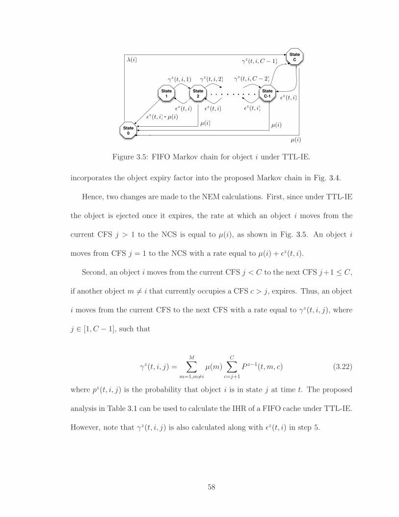
State
0
State
1
State
2
State
C-1
State
C
+
λ(i)
µ(i)µ(i) µ(i)
µ(i)
ǫz(t, i)
ǫz(t, i) ǫ
z(t, i) ǫz(t, i)
ǫz(t, i)
γz(t, i, 1) γ
z(t, i, 2) γz(t, i, C − 2)
γz(t, i, C − 1)
Figure 3.5: FIFO Markov chain for object i under TTL-IE.
incorporates the object expiry factor into the proposed Markov chain in Fig. 3.4.
Hence, two changes are made to the NEM calculations. First, since under TTL-IE
the object is ejected once it expires, the rate at which an object i moves from the
current CFS j > 1 to the NCS is equal to µ(i), as shown in Fig. 3.5. An object i
moves from CFS j = 1 to the NCS with a rate equal to µ(i) + ǫz(t, i).
Second, an object i moves from the current CFS j < C to the next CFS j+1 ≤ C,
if another object m 6= i that currently occupies a CFS c > j, expires. Thus, an object
i moves from the current CFS to the next CFS with a rate equal to γz(t, i, j), where
j ∈ [1, C − 1], such that
γz(t, i, j) =
M∑
m=1,m6=i
µ(m)
C∑
c=j+1
P z−1(t, m, c) (3.22)
where pz(t, i, j) is the probability that object i is in state j at time t. The proposed
analysis in Table 3.1 can be used to calculate the IHR of a FIFO cache under TTL-IE.
However, note that γz(t, i, j) is also calculated along with ǫz(t, i) in step 5.
58

3.4.3 FIFO Cache under TTL-T
For FIFO under TTL-T, expired objects are not ejected from the cache once they
expire. Rather, when an object i expires, the cache just marks it as an expired object.
Hence, the state of object i is modeled using the Markov chain in Fig. 3.6, where each
cache-fresh state (CFS) is associated with a cache-expired state (CES). In Fig. 3.6,
there are three types of states:
• Non-cache state (NCS): state 0, corresponds to when object i is not in the cache.
• Cache-fresh states (CFSs): odd states 1, 3, . . . , 2C−1, which correspond to when
object i is in the cache and the object is fresh.
• Cache-expired states (CESs): even states 2, 4, . . . , 2C, which correspond to when
object i is in the cache and the object is expired.
In Fig. 3.6, the total number of cache states is 2C. The state 2C − 1 is occupied
by the least recent object that entered the cache and is still fresh. Thus, when an
object i is in state 0, it moves to state 2C − 1 with rate λ(i). An object i moves from
the current CFS j to the associated CES j + 1, when it expires. The expired object
returns from CES j + 1 to CFS j when it is updated from the OS. Thus, an object i
moves from a CFS to the associated CES with rate µ(i), and returns from the CES to
the associated CFS with rate ς(i) = ηλ(i). Note that the validation factor, η, is the
probability that the request for an expired cached object (i.e. the validation request)
will be served from the OS (i.e. the object will be updated and the request will be
counted as a cache miss, as discussed in Section 1.1.1).
Furthermore, an object i moves from the current CFS to the previous CFS (e.g. from
59

State � State
1
State
3
State
State
State
2
2C − 3
State
4
2C − 1
State
2C − 2
State
2C
ǫz(t, i)
ǫz(t, i) ǫ
z(t, i) ǫz(t, i) ǫ
z(t, i)
ǫz(t, i)
ǫz(t, i)
ǫz(t, i) ǫ
z(t, i)
ǫz(t, i)
λ(i)
µ(i) µ(i) µ(i)
µ(i)ς(i)
ς(i)ς(i)ς(i)
Figure 3.6: FIFO Markov chain for object i under TTL-T.
state 3 to 1), or moves to the NCS (i.e. from state 1 to 0), when a cache miss occurs.
Thus, object i moves to the previous CFS, or to the NCS, with rate ǫz(t, i). Similarly,
object i moves from the current CES to the previous CES, or the NCS, with a rate
equal to ǫz(t, i).
For estimating the IHR of a single FIFO cache under TTL-T, the analysis in-
troduced in Table 3.1 is used, where ǫz(t, i), Pz(t, i), and Hz(t) are calculated us-
ing (3.18), (3.19), and (3.21), respectively. On the other hand, Sz(t, i) is calculated
after modifying (3.20), such that
Sz(t, i) = P z(t, i, 0) + η
C∑
j=1
P z(t, i, 2j) (3.23)
where P z(t, i, j) is calculated as
P z(t, i, j) = [Pz(t, i)]1,j+1 = [exp(Qz(t, i) t)]1,j+1 (3.24)
60

Also, the average validation request rate can be calculated at iteration z as
νz(t) =
M∑
i=1
λ(i)
C∑
j=1
P z(t, i, 2j) (3.25)
3.5 Analysis of LRU
In this section, a new analytical model of a single LRU cache is presented. The
proposed analysis assumes a stationary access pattern, as shown in Fig. 1.10(a). First,
the analysis for NEM is discussed in Section 3.5.1. Then, the analysis for TTL-IE
and TTL-T is discussed in Sections 3.5.2 and 3.5.3, respectively.
3.5.1 LRU Cache under NEM
Similar to the analysis in Section 3.4.1 for FIFO under NEM, the Markov chain in
Fig. 3.7 is used to model the state of object i for LRU under NEM. The Markov chain
in Fig. 3.7 has two types of states: NCS (state 0) and CFSs (states 1 to C).
In Fig. 3.7, the CFSs represent the relative time at which object i was requested.
State C corresponds to the most recently requested object. The recency of a requested
object decreases as the object goes from CFS j to CFS j − 1. State 1 corresponds to
the least recently requested object.
In Fig. 3.7, an object i moves from the current state j ∈ [1, C − 1] to state C
with rate λ(i) (i.e. when object is requested). Also, object i moves from state C to
state C − 1 when any other object is requested (with rate β − λ(i)). Furthermore,
an object i moves from the current state j to the next lower-numbered one when
an object occupying a state w ≤ j is requested. Thus, the rate at which a cached
61

State
0
State
1
State
2
State
C-1
State
C
λ(i)
λ(i)λ(i)
β − λ(i)
ǫz(t, i, 1)
ǫz(t, i, 2) ǫ
z(t, i, 3) ǫz(t, i, C − 1)
Figure 3.7: LRU Markov chain for object i under NEM.
object i moves from the current state to the next lower-numbered one, ǫz(t, i, j), can
be calculated as
ǫz(t, i, j) =M
∑
m=1,m6=i
λ(m)
j∑
c=0
P z−1(t, m, c) (3.26)
Similar to FIFO under NEM, the analysis proposed in Table 3.1 is used for es-
timating the IHR of LRU under NEM, such that ǫz(t, i, j) is calculated in step 5
using (3.26).
3.5.2 LRU Cache under TTL-IE
Like the analysis for FIFO under TTL-IE, the analysis for LRU under TTL-IE ac-
counts for the object expiry by introducing two main changes to the Markov chain
shown in Fig. 3.7. First, the rate at which an object i moves from the current CFS to
NCS is increased by µ(i), as shown in Fig. 3.8. Second, an object i moves from the
current CFS j < C to the next CFS j +1 ≤ C, if another object m 6= i that currently
occupies a cache state c > j expires. Thus, an object i moves from the current CFS
to the next CFS with rate equal to γz(t, i, j), which is calculated using (3.22), where
62

j ∈ [1, C − 1]. Note that, in Fig. 3.8, ǫz(t, i, j) is calculated using (3.26).
State
0
State
1
State
2
State
C-1
State
C
+
+
λ(i)
λ(i)λ(i)
β − λ(i)
ǫz(t, i, 1)
ǫz(t, i, 2) ǫ
z(t, i, 3) ǫz(t, i, C − 1)
µ(i)µ(i)
µ(i)
µ(i)
γz(t, i, 1) γ
z(t, i, 2) γz(t, i, C − 2)
γz(t, i, C − 1)λ(i)
Figure 3.8: LRU Markov chain for object i under TTL-IE.
Like FIFO under TTL-IE, the analysis shown in Table 3.1 can be used to calculate
the IHR of LRU under TTL-IE, where γz(t, i, j) and ǫz(t, i, j) are in step 5.
3.5.3 LRU Cache under TTL-T
Like FIFO under TTL-T, the analysis proposed in the previous section can be modi-
fied for LRU under TTL-T by associating a CES to each CFS, as shown in the Markov
chain in Fig. 3.9.
In Fig. 3.9, the state 2C − 1 is occupied by the most recently requested object,
if the object is fresh. Thus, when an object i is requested from any CFS, it moves
to state 2C − 1 with rate λ(i). Also, when an object i is requested from any CES, it
moves to state 2C − 1 with rate ς(i) = ηλ(i). Note that the state 2C is occupied by
the most recently requested object, assuming that the object is expired. Thus, when
an object i is requested from any CES, it moves to state 2C with rate λi − ς(i).
Moreover, an object i in state 2C − 1, or state 2C, moves to the previous state
with rate β − λ(i) (i.e. if any object other than i is requested). An object i moves
63

State
0
State
1
State
3
State
State
State
2
State
4
2C − 3
2C − 1
State
2C − 2
State
2C
ǫz(t, i, 3)
ǫz(t, i, 2)
λ(i)
λ(i) λ(i) λ(i)
µ(i) µ(i) µ(i) µ(i)
λ(i)
ǫz(t, i, 2C − 3)
β − λ(i)
β − λ(i)
ǫz(t, i, 1)
ǫz(t, i, 4) ǫ
z(t, i, 2C − 2) λ(i) − ς(i)
ς(i)
ς(i)
Figure 3.9: LRU Markov chain for object i under TTL-T.
from the current CFS j to the associated CES j +1, when it expires. Thus, an object
i moves from a CFS to the associated CES with rate µ(i).
An object i moves from the current CFS j to the previous CFS j − 1 (e.g. from
state 3 to 1), or moves to the NCS (i.e. from state 1 to 0), when an object that
occupies state c < j, is requested. Thus, object i moves to the next lower CFS, or to
the NCS, with a rate that is equal to ǫz(t, i, j), where j is odd, such that
ǫz(t, i, j) =
M∑
m=1,m6=i
λ(m)
j+1∑
c=0
P z−1(t, m, c) for odd j (3.27)
Similarly, object i moves from the current CES to the next lower CES, or to the
NCS, with rate ǫz(t, i, j), which is calculated using (3.26), where j is even.
Similar to FIFO under TTL-T, the analysis proposed in Table 3.1 is used for
estimating the IHR of LRU under TTL-T, where Sz(t, i), P z(t, i, j), and νz(t) are
calculated according to (3.23), (3.24), and (3.25), respectively.
64

3.6 Generalized Analysis of a Non-stationary Access Pattern
In the previous sections, the proposed analysis assumed a stationary access pattern,
where the access pattern is fixed from the moment that an empty cache starts to
operate until the cache reaches the SSHR, as described in Section 1.2. In this section,
the extension of the proposed analysis for a non-stationary access pattern is presented.
In a non-stationary access pattern, the access pattern characteristics may change
after, or before, the cache reaches the SSHR, as shown in Figs. 1.10(b, c). Particularly,
this section shows how the proposed analysis can be generalized for estimating the
IHR, assuming new popular objects are periodically generated at the OS.
This section is organized as follows. The analysis of Infinite Cache under a non-
stationary access pattern is proposed in Section 3.6.1. Then, the analysis of FIFO
and LRU under a non-stationary access pattern is presented in Section 3.6.2.
3.6.1 Generalized Analysis of Infinite Cache
For Infinite Cache under a non-stationary access pattern, the IHR is calculated us-
ing (3.1) for NEM, TTL-IE, or TTL-T. However, the following modifications to the
analysis presented in Section 3.2 are required:
1- Assuming that the number of objects changes at time tv to M(tv), if the number
of objects remains fixed within the time interval (tv, t1), then the probability matrix
of object i at time t1, P(t1, i), is calculated by modifying (3.2) to
P(t1, i) = exp(Q(i) ∆t) (3.28)
65

time
time
t0
∆t = t1 − t0
∆t = t1 − tv
P (tv, i, j),∀i, j
P (t0, i, j),∀i, j
t1
t1
tv
P (t0, i, j),∀i, j
t0
S(t1, i)
S(t1, i)
Figure 3.10: Calculating S(t1, i), assuming stationary access pattern within the in-terval (t1, t1 − ∆t).
where ∆t = t1 − tv and t1 > tv. Note that (3.28) is used for NEM, TTL-IE, and
TTL-T.
2- S(t1, i) has to be calculated based on the probabilities P (tv, i, j), ∀i, j. Note
that S(t1, i) cannot be calculated based on the probabilities P (t0 = 0, i, j), ∀i, j (i.e.
S(t1, i) cannot be calculated using (3.5)), if the access pattern is not stationary within
the interval (t0, t1), as shown in Fig. 3.10. Therefore, for NEM and TTL-IE, S(t1, i)
is calculated by modifying (3.5) to (3.29). Similarly, for TTL-T, S(t1, i) is calculated
by modifying (3.9) to (3.30).
S(t1, i) =
2∑
r=1
[P(t1, i)]r,1 P (tv, i, r − 1) (3.29)
S(t1, i) =
3∑
r=1
[P(t1, i)]r,1 P (tv, i, r − 1) + η
3∑
r=1
[P(t1, i)]r,3 P (tv, i, r − 1) (3.30)
66

3.6.2 Generalized Analysis of FIFO and LRU
Similar to Infinite Cache, Pz(t1, i) can be calculated for FIFO and LRU by modify-
ing (3.19) to
Pz(t1, i) = exp(Qz(i) ∆t)
where ∆t = t1 − tv. Then, Sz(t1, i) is calculated for NEM or TTL-IE by modify-
ing (3.20) to
Sz(t1, i) =C+1∑
r=1
[Pz(t1, i)]r,1 P ∗(tv, i, r − 1)
where the superscript (.)∗ indicates the final fixed point state probability solution
provided by the contraction mapping analysis in Section 3.5. Similarly for TTL-T,
S(t1, i) is calculated by modifying (3.23) to
Sz(t1, i) =
2C+1∑
r=1
[Pz(t1, i)]r,1 P ∗(tv, i, r− 1)+ η
2C∑
j=1
2C+1∑
r=1
[Pz(t1, i)]r,2j+1 P ∗(tv, i, r− 1)
3.7 FB-FIFO Replacement Policy
Unlike Perfect-LFU, LRU and FIFO do not store any information about the pop-
ularity of objects (i.e. number of requests), whether they are currently cached or
not. Hence, LRU and FIFO can be easily implemented with a linked list, with length
C. However, compared to FIFO, LRU requires more overhead on every cache hit
to an object in order to change its state to C (i.e. to move it to the front of the
list as the most recently requested object) [46, 87, 148]. Many replacement policies
67

are introduced in order to enhance the SSHR of LRU, such as LRU-k, ARC, and
LRFU [92, 98, 149]. However, these policies are even more complex than LRU, and
they require additional resources.
In Section 3.4.1, the Markov chain representation of FIFO showed that the hit
ratio degrades because FIFO allows all new objects, unpopular or not, to occupy state
C. State C is the position in the chain that allows the object to remain in the cache
for the maximum amount of time. In this section, this insight is used to develop an
improved version of FIFO policy, called frequency-based-FIFO (FB-FIFO).
The main idea behind FB-FIFO is to create a variable-sized protected segment in
the cache (Sp) for objects that are not effectively one-timers. The object is effectively
a one-timer if it cannot generate a cache hit, either due to its low request rate, or
because it is requested only once throughout the cache operation3. The remainder
of the cache is considered an unprotected segment (Su). In FB-FIFO, it is assumed
that both cache segments are managed separately with the FIFO policy. When an
uncached object is requested, the object is moved to Su as the newest object. If Su is
full, then the object that was brought into Su earliest will be ejected from the cache,
as shown in Fig. 3.11.
If an object in Su experiences a cache hit (the object is not effectively a one-
timer), the object is moved to Sp as the newest object. If Sp is full, the object
that was brought into Sp the earliest will move back to Su as the newest object. A
3A one-timer is an object that is requested once, and will never be requested again. The objectis effectively a one-timer if it is requested once, or if it is requested more than once but the timeintervals between requests are longer than the durations that the object lingers in the cache. Hence,the object that is effectively a one-timer cannot generate a cache hit.
68

a b c di
Su Sp
ab c d i
C
(1) Request for
an object
(2) Cache ejects
object
e f g h
e f g h
Oldest
ObjectNewest
Object
Oldest
ObjectNewest
Object
Figure 3.11: FB-FIFO: a new object enters the cache.
counter, n, determines the capacity of Sp, while the capacity of Su is C − n, such
that 0 ≤ n ≤ Nmax, and Nmax < C. The initial value of n is set to zero at time
t = 0. Every time an object in Su experiences a cache hit, the value of n increments
by one if n < Nmax. If n = Nmax, n cannot increment further, as shown in Fig. 3.12.
Note that, under TTL-IE, if an object in Sp expires, it will be ejected from the cache
and the value of n decrements by one. However, under NEM or TTL-T, n does not
decrement. Note that objects in Sp do not move back to Su if n < Nmax. A flow
chart of FB-FIFO is illustrated in Fig. 3.13.
As n increases, the probability that a new cached object lingers in Su decreases.
When a new object is cached in Su, it will be ejected if the next C − n requests
are all cache misses. Therefore, as n increases, the probability that the objects that
are moved to Sp (as the newest objects) are popular increases. Furthermore, the
objects that are effectively one-timers will not affect the Sp queue. Hence, FB-FIFO
is expected to outperform FIFO, which can easily be polluted by a sequence of requests
for objects that are effectively one-timers.
69

0
C = 8
Nmax = 7
a b c d e f g h
(1) Request for
an object
b
SuSp
(2) Move Object
f g hedca b
to head of Sp
n = 4
n = 5(3) Increment
b
(a) if n < Nmax.
0
C = 8
a b c d e f g h
b
SuSp
(2) Move Object
f g hedca b
to head of Sp
n = Nmax = 4
b
(3) Move Object
to head of Su
e
(1) Request for
an object
(b) if n = Nmax.
Figure 3.12: FB-FIFO: an object in Su is accessed.
FB-FIFO allows the current popular objects to be cached in Sp. In FB-FIFO,
any object moves from Su to Sp when it is requested within the next C − n requests
(excluding cache hits), regardless of the past average request rate of this object.
Therefore, FB-FIFO is expected to adapt faster than Perfect-LFU to the changes in
the popularity of the cached objects (i.e. FB-FIFO is more robust than Perfect-LFU),
especially when the cached objects accumulate many requests over time. In this case,
Perfect-LFU does not eject these cached objects, even if they are never requested
70

Yes, cache hit
Request for an object
Is the requested object in cache ?
No, cache miss
cache full ?
Yes
No
- Move objects from state j to j-1, for all j in [2, C-n]- Cache requested object in state C-n
Eject objectfrom state 1
Is the requested object in a state w is protected ?
Request process ends
Yes, object is protected, and w in [C-n+1, C]
n < N_max ?
Yes
n=n+1
Initially, n=0
No
- Move objects from state j to j-1, for all j in [w+1, C-n]- Move objects from state j to j-1, for all j in [C-n+1, C]
- Cache requested object in state C
No, object is not protected, and w in
[1, C-n]
Figure 3.13: FB-FIFO flow chart.
again. LFU-Aging [14] overcomes this problem by periodically reducing the counter
values associated with cached objects.
The robustness of FB-FIFO may also decrease for small cache capacities, when n
reaches Nmax and does not decrease (i.e. under NEM and TTL-T, where n cannot
decrease). If n = Nmax = C − 1, only very popular objects can replace the past
popular objects in Sp, since a single object in Su is ejected on the next cache miss. To
overcome this problem, more complicated versions of FB-FIFO may be implemented
to reset n to zero after a certain number of cache misses. In this chapter, the simplest
version of the proposed FB-FIFO is evaluated, where n decreases under TTL-IE if and
only if a cached object in Sp expires, while n does not decrease under NEM or TTL-
T. Note that, under TTL-IE, as the object expiry rate increases, the robustness of
FB-FIFO improves for small caches, since FB-FIFO under TTL-IE allows the expired
71

past popular objects in Sp to be ejected from the cache.
Note that determining a static value for n = Nstatic (i.e. fixed capacities for Su
and Sp throughout the evaluation interval) reduces the IHR of FB-FIFO. If Nstatic is
increased, the speed at which Sp fills up decreases. Consequently, the IHR increases
very slowly in the transient period starting from an empty cache. If Nstatic is de-
creased, the number of popular objects that can be stored in Sp decreases. Thus, the
IHR for FB-FIFO decreases as Nstatic decreases, until FB-FIFO matches FIFO when
Nstatic = 0.
3.8 Evaluation of the IHR under NEM and TTL-IE
An event-driven simulator was developed using C++ to verify the analytical results for
Infinite Cache, LRU, and FIFO. Also, FB-FIFO and Perfect-LFU are implemented in
the simulations to allow a comparison with LRU and FIFO. The workload generator is
used to generate 1000 workload profiles that statistically conform with the proposed
mathematical models in Section 3.1. For each simulated workload, the simulator
determines the IHR at every simulation timestep, δt. The final simulated IHR is then
determined by averaging the IHR for all 1000 simulated profiles4 at each simulation
timestep. For example, let Hsimulation(t, n) denote the simulated IHR that is generated
using the nth workload profile at time t. The final simulated IHR using N workload
4This large number of runs is required for achieving 95% confidence interval with maximum errorof estimate [71] that is lower than 0.3%.
72

profiles is calculated as
Hsimulation(t)|N =1
N
N∑
n=1
Hsimulation(t, n) (3.31)
The IHR, H(t), is calculated over a duration of 3 to 20 hours in δt = 0.25 hour
intervals as a function of cache capacity, object expiry rate, and request rate. Note
that the analysis estimates the IHR at a specific time t, while the simulated IHR
using the nth profile, Hsimulation(t, n), is the time domain average of the hit ratio over
the interval δt (i.e. the number of cache hits divided by the total number of requests
within δt), as shown in Fig. 3.14.
δt
time
δt
t1 t2
Requests =
1000
Hits
= 500Requests =
1000
Hits
= 250
H(t2, n) = 25%H(t1, n) = 50%
Figure 3.14: Simulated IHR is calculated at every simulation timestep, δt.
In the analysis and simulations, the ratio between the cache size and the average
object size (i.e. the cache capacity C) varies from 100 to 500. Though the analysis
estimates the IHR assuming objects with different expiry rates, for simplicity, the
IHR is evaluated in this chapter assuming that all the objects have the same expiry
rate, µe = µ(i) ∀i ∈ [1, M ]. The request rates vary from 200 to 500 requests/hr, and
are chosen such that the evolution of the IHR can be captured in the transient state.
73

The analysis and the simulator adopt the settings shown in Table 3.2. Note that the
values in Table 3.2 are intended to illustrate the concepts in this chapter rather than
representing empirical workload values.
Table 3.2: SCS: IHR evaluation factors and levels.
Factor Symbol ValueNumber of Objects M 5000 - 10,000
Time Duration T 3 - 20 hoursSimulation Timestep δt 0.25 hour
Zipf Slope α 0.8 [11, 14]Cache Capacity C 100, 300, 500, Infinite Cache
Object Expiry Rate µe 0.5, 1 per hour [150]Request Arrival Rate β 200 - 500 per hour
In Section 3.8.1, the considered replacement policies are evaluated, assuming a
stationary access pattern, with a fixed number of objects at the OS (M = 10, 000).
Section 3.8.2 illustrates the evaluation of replacement policies, assuming that the OS
generates new popular objects periodically (i.e. a non-stationary access pattern is
assumed). In the following, all plots show the hit ratio as a function of time (i.e.
IHR). The markers in these plots represent the simulation results, while analysis
results that correspond to each simulated scenario are shown with solid lines.
3.8.1 Evaluation of Replacement Policies under a Stationary Access Pattern
In this section, the IHR, H(t), is plotted within interval [0, T ] starting from an empty
cache at time t = 0, where T = 210 minutes. Within this interval, it is assumed that
the number of objects and the Zipf slope are fixed (M = 10, 000, α = 0.8).
Fig. 3.15 shows a close match between analysis and simulation results for Infinite
Cache, LRU, and FIFO assuming a cache capacity of C = 500, cached objects that
74

do not expire (i.e. µe = 0), and request rate of β = 500. This plot also indicates
that the hit ratio of the different replacement policies evolve differently as a function
of time. In Fig. 3.15, Infinite Cache, LRU, FIFO, FB-FIFO, and Perfect-LFU have
the same hit ratio until tfull = 75 minutes, where tfull denotes the time when the
cache becomes full. After tfull, the replacement policy starts replacing some cached
objects, causing the hit ratio to increase in case of LRU, FB-FIFO, and Perfect-LFU,
or decrease in case of FIFO.
0 30 60 90 120 150 180 210
10
20
30
40
50
Hit
ratio
%
Time (minutes)
Infinite CachePerfect−LFUFB−FIFOLRUFIFO
Figure 3.15: IHR, where C = 500, µe = 0, and β = 500.
Unlike the other replacement policies, Fig. 3.15 shows that FIFO reaches a max-
imum hit ratio of 31.4% during the transient period. Afterwards, FIFO decreases
again and keeps fluctuating until reaching the SSHR of 29.4% after 210 minutes.
Unlike the other replacement policies, FIFO does not exploit the popularity feature
of objects. Thus, it is likely that some of the most popular objects that are cached
within the first 30 minutes will reside at low cache states at tfull. Note that the
hit ratio increases rapidly within the first 30 minutes when a big percentage of the
most popular objects are cached. Hence, FIFO starts replacing a portion of the most
popular objects with less popular ones after tfull, which causes the hit ratio to drop.
75

Afterwards, the hit ratio will increase again as FIFO starts caching the most popular
objects, which could be replaced after tfull, again. An oscillation in hit ratio continues
to be observed as the most popular objects work their way through the cache and
get ejected. Eventually, steady state is reached once FIFO is able to maintain a fixed
percentage of the most popular objects in the cache.
Fig. 3.15 shows that the proposed FB-FIFO outperforms both LRU and FIFO,
while FB-FIFO achieves the same hit ratio as Perfect-LFU during the evaluation
interval [0, T ]. Note that Perfect-LFU and FB-FIFO start outperforming LRU at
time t = 120 minutes. Before tfull, the three replacement policies maintain the same
objects in the cache. However, unlike Perfect-LFU and FB-FIFO, LRU suffers from
requests for objects that are effectively one-timers, which constrains the increase in
the percentage of the cached popular objects after tfull.
The remainder of this section discusses the impact of cache capacity, object expiry,
and request rate on the considered replacement policies.
Impact of Cache Capacity
Fig. 3.16 shows the impact of cache capacity, C, on H(t) for the considered replace-
ment policies. Fig. 3.16 shows that as C decreases, the cache fills up quickly and
thus, Perfect-LFU, FB-FIFO, and LRU start outperforming FIFO sooner.
Fig. 3.16(a) shows that FIFO fluctuates more rapidly and reaches steady state
faster when C decreases to 300. Table 3.3 helps illustrating the behavior for FIFO.
Fig. 3.16(b) shows that when C decreases to 100, FIFO fluctuation diminishes. When
C decreases, the percentage of the most popular objects that are cached when the
76
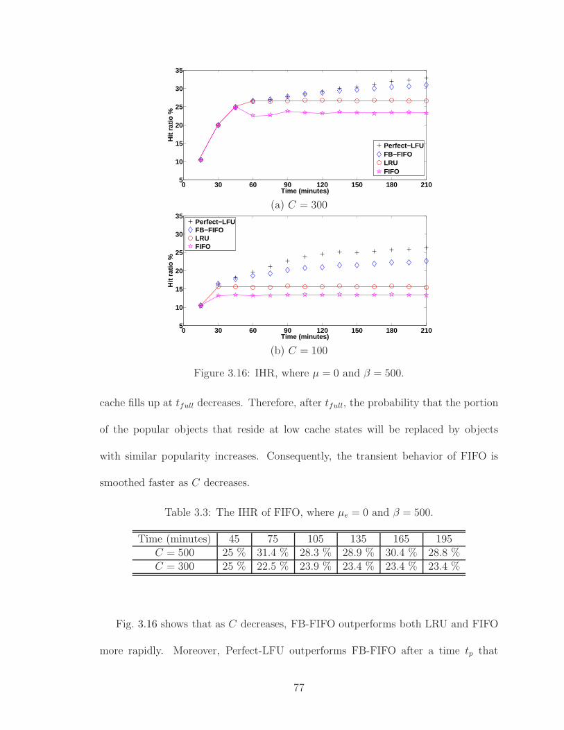
0 30 60 90 120 150 180 2105
10
15
20
25
30
35
Hit
ratio
%
Time (minutes)
Perfect−LFUFB−FIFOLRUFIFO
(a) C = 300
0 30 60 90 120 150 180 2105
10
15
20
25
30
35
Hit
ratio
%
Time (minutes)
Perfect−LFUFB−FIFOLRUFIFO
(b) C = 100
Figure 3.16: IHR, where µ = 0 and β = 500.
cache fills up at tfull decreases. Therefore, after tfull, the probability that the portion
of the popular objects that reside at low cache states will be replaced by objects
with similar popularity increases. Consequently, the transient behavior of FIFO is
smoothed faster as C decreases.
Table 3.3: The IHR of FIFO, where µe = 0 and β = 500.
Time (minutes) 45 75 105 135 165 195C = 500 25 % 31.4 % 28.3 % 28.9 % 30.4 % 28.8 %C = 300 25 % 22.5 % 23.9 % 23.4 % 23.4 % 23.4 %
Fig. 3.16 shows that as C decreases, FB-FIFO outperforms both LRU and FIFO
more rapidly. Moreover, Perfect-LFU outperforms FB-FIFO after a time tp that
77

decreases with C, for example, tp = 120 when C = 300, whereas tp decreases to 30
when C = 100. Note that if any replacement policy keeps a similar percentage of the
popular objects as Perfect-LFU, that replacement policy achieves a hit ratio similar
to Perfect-LFU. Therefore, after tfull, the difference between Perfect-LFU and FB-
FIFO is small. This difference increases over time as Perfect-LFU identifies more of
the popular objects. As C increases, it takes longer for Perfect-LFU to distinguish
popular objects with request rate that are too low to be identified by FB-FIFO. Thus,
FB-FIFO tracks Perfect-LFU for a longer time.
Impact of Object Expiry Rate
Fig. 3.17 shows the impact of the object expiry rate, µe, on H(t). Fig. 3.17 shows
that as µe increases, H(t) decreases since the rate at which the object is ejected from
the cache increases. Moreover, H(t) reaches steady state faster as µe increases. Also,
note that the transient behavior of FIFO diminishes as µe increases. As discussed
in Section 3.8.1, this is due to the decrease in the percentage of the most popular
objects that are cached when the cache fills up.
Let H(t, 1) and H(t, 2) denote the IHR in Fig. 3.17(a) and Fig. 3.17(b), respec-
tively. Fig. 3.18 shows the relative change in the IHR (i.e. (H(t, 1)−H(t, 2))/H(t, 1)).
In Fig. 3.18, the results show that Infinite Cache is the most sensitive to µe, followed
by Perfect-LFU, FB-FIFO, LRU, and FIFO. As µe increases, the popular objects are
ejected due to object expiry, rather than requests for uncached objects. Thus, the
replacement policies that minimize the ejection of popular objects are more sensitive
to µe.
78

0 30 60 90 120 150 180 2105
10
15
20
25
30
35
Hit
ratio
%
Time (minutes)
Infinite CachePerfect−LFUFB−FIFOLRUFIFO
(a) µe = 0.5
0 30 60 90 120 150 180 2105
10
15
20
25
30
35
Hit
ratio
%
Time (minutes)
Infinite CachePerfect−LFUFB−FIFOLRUFIFO
(b) µe = 1
Figure 3.17: IHR, where C = 300 and β = 500.
Impact of Request Rate
Figs. 3.19 and 3.17(a) show that, in the transient state, the IHR for all the replacement
policies decreases when β decreases to 250 requests/hr, while µe = 0.5. This is
consistent with the results for the SSHR of Infinite Cache generated in [11]. Moreover,
comparing Figs. 3.19 and 3.17(a) shows that the relative increase in β with respect to
µe improves FB-FIFO more rapidly than LRU and FIFO, which improves the least.
Comparing Figs. 3.19 and 3.17(b) shows that doubling β and µe for a replacement
policy results in the same SSHR. However, the steady state is reached faster. For
example, Perfect-LFU, FB-FIFO, and LRU reach steady state at time t = 90 when
β = 500, while the time required to reach steady state is almost doubled when
79

0 30 60 90 120 150 180 210
−0.2
−0.1
0
0.1
0.2
0.3
Hit
ratio
%
Time (minutes)
Infinite CachePerfect−LFUFB−FIFOLRUFIFO
Figure 3.18: The relative change in the IHR when µe increases from 0.5 to 1, whereC = 300 and β = 500.
0 30 60 90 120 150 180 2105
10
15
20
25
30
35
Hit
ratio
%
Time (minutes)
Infinite CachePerfect−LFUFB−FIFOLRUFIFO
Figure 3.19: IHR, where C = 300, µe = 0.5, and β = 250.
β = 250.
3.8.2 Evaluation of Replacement Policies under a Non-stationary Access Pattern
In this section, the IHRs of the replacement policies are evaluated over T = 20 hours,
assuming that the initial number of objects at time t = 0 is M(t = 0) = 5000. Every
∆T = 5 hours, 50 new objects are generated. It is assumed that the 50 new generated
objects become the most popular objects within the next ∆T . For example, the most
popular object within the interval [0, 5] hours becomes the 50th most popular object
within the interval (5, 10] hours, and the 100th most popular object within the interval
(10, 15] hours. Similarly, the most popular object that is generated at t = 5 hours
80

becomes the 50th most popular object within the interval (10, 15] hours, and so on.
Therefore, the initial popularity of the cached objects degrades over time.
Fig. 3.20 shows that the analysis accurately estimates the IHR of LRU and FIFO,
assuming a non-stationary access pattern. Also, Fig. 3.20 illustrates the case when
the cache does not reach steady state. Hence, the only way to estimate the hit ratio
experienced by Web users is to calculate the IHR.
0 2.5 5 7.5 10 12.5 15 17.5 205
10
15
20
25
30
35
Hit
ratio
%
Time (Hours)
Perfect−LFUFB−FIFOLRUFIFO
(a) µe = 0
0 2.5 5 7.5 10 12.5 15 17.5 205
10
15
20
25
30
Hit
ratio
%
Time (Hours)
Perfect−LFUFB−FIFOLRUFIFO
(b) µe = 0.5
Figure 3.20: IHR, where C = 100 and β = 200.
Fig. 3.20(a) shows that for C = 100, FB-FIFO adapts faster than the other
replacement policies when new objects are generated at time t = 5 hours. Assume
that the robustness of the replacement policy is denoted by the IHR achieved shortly
after M(t) changes (for example, H(t = 5.5) after M(t) changes at t = 5). Fig. 3.20(a)
81

shows that FB-FIFO is the most robust replacement policy after t = 5 hours. After
t = 10, 15 hours, LRU becomes the most robust replacement policy followed by FIFO,
FB-FIFO, and then Perfect-LFU. At C = 100, the popularity of the cached objects
decreases greatly for Perfect-LFU and FB-FIFO every time 50 new popular objects
are generated. Hence, Perfect-LFU and FB-FIFO degrade greatly over time since
they take longer to eject formerly popular objects. As discussed in Section 3.7, after
t = 15 hours, it might be useful for FB-FIFO to reset the counter to zero, or decrease
its counter value on every cache miss, which may help remove old popular objects
faster. Also, as discussed in Section 3.7, as µe increases, FB-FIFO becomes more
robust, as shown in Fig. 3.20(b).
Note that the ratio between the number of new popular objects and the cache ca-
pacity plays a key role in the relative robustness of the replacement policies. Fig. 3.21(a)
shows that as C increases to 300, after t = 10, 15 hours, FB-FIFO becomes the most
robust replacement policy followed by LRU, Perfect-LFU, and FIFO. The relative ro-
bustness of FB-FIFO increases each time new objects are generated. As discussed in
Section 3.7, FB-FIFO caches the current popular objects in Sp faster as C increases,
regardless of the past request rate of these objects.
Fig. 3.21(b) shows that as C increases to 500, FB-FIFO matches Perfect-LFU for a
longer time starting from an empty cache at time t = 0, as discussed in Section 3.8.1.
Furthermore, Figs. 3.21(a, b) show that after t = 15 hours, FB-FIFO outperforms
Perfect-LFU for a longer duration when C increases from 300 to 500. As discussed in
Section 3.7, Perfect-LFU is affected more than FB-FIFO when more cached objects
accumulate many requests over time. In this case, Perfect-LFU takes longer than
82

0 2.5 5 7.5 10 12.5 15 17.5 205
10
15
20
25
30
35
40
45
Hit
ratio
%
Time (Hours)
Perfect−LFUFB−FIFOLRUFIFO
(a) C = 300
0 2.5 5 7.5 10 12.5 15 17.5 20
10
20
30
40
50
Hit
ratio
%
Time (Hours)
Perfect−LFUFB−FIFOLRUFIFO
(b) C = 500
Figure 3.21: IHR, where µe = 0 and β = 200.
FB-FIFO to identify the new popular objects and get rid of the old ones.
3.9 Evaluation of the SSHR under TTL-IE and TTL-T
This section evaluates the steady state hit ratio (SSHR) of FIFO, LRU, and FB-FIFO,
assuming a stationary access pattern. The analysis and simulator adopt the settings
shown in Table 3.4. The values in this table are meant to illustrate the concepts in
this section, and they are not taken directly from empirical workload values.
In the following, all plots show the SSHR as a function of the cache capacity, C.
Note that the markers in these plots represent the simulation results, while analysis
results are shown with solid lines.
83

Table 3.4: SCS: SSHR evaluation factors and levels.
Factor Symbol ValueNumber of Objects M 1000
Zipf Slope α 0.8 [14, 11]Aggregate Request Arrival Rate β 200 per hour
Cache Capacity C 20-100Object Expiry Rate µe 10, 1 per hour [150]Validation Factor η 0.2, 0.5, 0.8
Fig. 3.22(a) shows the SSHR of FIFO at µe = 10 (relatively high expiry rate [150]).
Fig. 3.22(a) shows that the SSHR for TTL-IE slightly outperforms the one for TTL-
T when C is small (e.g. 20) and η is high (e.g. 0.8). Fig. 3.22(a) shows that as C
increases, or η decreases, the SSHR for TTL-T improves faster than for TTL-IE.
This is because as C increases, TTL-IE does not make full use of the available cache
capacity since the cached objects are ejected once they expire. On the other hand,
TTL-T allows expired objects to stay in the cache, which results in an increased
number of cache hits, especially when η is small.
Fig. 3.22(b) shows the SSHR of FIFO at µe = 1 (i.e. relatively moderate expiry
rate). Fig. 3.22(b) shows that both TTL-T and TTL-IE yield similar SSHR when the
cache is small, regardless of η. This is because ejections due to caching new objects
dominate ejections due to object expiry in TTL-IE. Fig. 3.22(b) shows that as C
increases, the SSHR for TTL-IE outperforms the one for TTL-T even for a low η
(e.g. 0.2). This is because TTL-IE allows the cache to eject unpopular objects from
the FIFO queue faster, while TTL-T wastes the cache capacity by keeping the expired
unpopular objects in their regular order in the FIFO queue.
Fig. 3.23 shows that the SSHR of LRU acts like FIFO for both TTL implemen-
84

20 40 60 80 1005
10
15
20
25
30
Cache Capacity
Hit
ratio
%
TTL−IETTL−T, η=0.2TTL−T, η=0.5TTL−T, η=0.8
(a) µe = 10
20 40 60 80 10010
15
20
25
30
35
Cache Capacity
Hit
ratio
%
TTL−IETTL−T, η=0.2TTL−T, η=0.5TTL−T, η=0.8
(b) µe = 1
Figure 3.22: SSHR of FIFO.
tations. The only difference appears in Fig. 3.23(b) at µe = 1 and η = 0.2, where
the SSHR of LRU under TTL-T matches the SSHR of LRU under TTL-IE, when
C < 80. Also, for LRU, the SSHR under TTL-T is better than the SSHR under
TTL-IE, when C ≥ 80. This is because, under TTL-T, LRU allows unpopular ob-
jects to be ejected faster than FIFO, since LRU reorders the cache queue according
to recency (or popularity, since a stationary access pattern is assumed [11]).
Fig. 3.24 shows that FB-FIFO outperforms LRU and FIFO under TTL-T when
the cache is small, as suggested by the results in Section 3.8.1. Fig 3.24 shows that the
SSHR of FB-FIFO degrades rapidly under TTL-IE as µe increases. This is consistent
with the results in Section 3.8.1.
85

20 40 60 80 1005
10
15
20
25
30
35
Cache Capacity
Hit
ratio
%
TTL−IETTL−T, η=0.2TTL−T, η=0.5TTL−T, η=0.8
(a) µe = 10
20 40 60 80 10010
15
20
25
30
35
40
Cache Capacity
Hit
ratio
%
TTL−IETTL−T, η=0.2TTL−T, η=0.5TTL−T, η=0.8
(b) µe = 1
Figure 3.23: SSHR of LRU.
Under TTL-T, Figs. 3.23 and 3.24 show that, compared to the SSHR of LRU,
the SSHR of FB-FIFO is very sensitive to the value of η. For example, Figs. 3.23(a)
and 3.24(a) show that when µe = 10 and C = 20, the SSHR of LRU increases by 3%,
in case of LRU, and increases by 10%, in case of FB-FIFO, when η decreases from
0.8 to 0.2.
Moreover, Fig. 3.24(b) shows that the sensitivity of FB-FIFO to η decreases more
rapidly than LRU as µe decreases (i.e. as the probability of objects being in a CES
decreases). For example, Figs. 3.23(b) and 3.24(b) show that when µe = 1 and
C = 20, the SSHR of LRU increases by 0.3%, in case of LRU (i.e. the sensitivity
to η decreases by 2.7% compared to when µe = 10), and increases by 3%, in case of
86

FB-FIFO (i.e. the sensitivity to η decreases by 7% compared to when µe = 10), when
η decreases from 0.8 to 0.2.
20 40 60 80 1005
10
15
20
25
30
35
40
Cache Capacity
Hit
ratio
%
TTL−IETTL−T, η=0.2TTL−T, η=0.5TTL−T, η=0.8
(a) µe = 10
20 40 60 80 10010
15
20
25
30
35
40
45
Cache Capacity
Hit
ratio
%
TTL−IETTL−T, η=0.2TTL−T, η=0.5TTL−T, η=0.8
(b) µe = 1
Figure 3.24: SSHR of FB-FIFO.
Note that, under TTL-T, FB-FIFO protects the popular objects from being
ejected (i.e. FB-FIFO cached popular objects in the protected segment Sp), even
after they expire, as discussed in Section 3.7. Hence, the SSHR of FB-FIFO is very
sensitive to the probability that the expired protected objects are invalid, η, as well
as the object expiry rate, µe. On the other hand, compared to FB-FIFO, LRU allows
more expired popular objects to be ejected, which is why LRU is less sensitive to η
and µe.
87

3.10 Summary
In this Chapter, the proposed analytical models for Infinite Cache, Perfect-LFU,
FIFO, and LRU were presented. Then, a new replacement policy, FB-FIFO, was
introduced. In Section 3.8, the replacement policies were evaluated under NEM and
TTL-IE. The results in Section 3.8 showed that different replacement policies have
very different transient performance, whether the popularity of cached objects is fixed
or not. This makes the proposed analysis in this chapter valuable when considering
scenarios like changing popularity or mobile caching. The following list summarizes
the major findings in Section 3.8:
• For a stationary access pattern, where the number of objects and the object
popularity are fixed during the transient period:
1- Unlike the other replacement policies studied in this chapter, FIFO reaches
its maximum hit ratio during the transient fluctuations that occur before reaching
steady state. These fluctuations diminish as the cache capacity decreases, or as the
object expiry rate increases with respect to the request rate.
2- FB-FIFO outperforms both LRU and FIFO, especially when cache capacity
is small. Moreover, FB-FIFO matches Perfect-LFU for a longer time as the cache
capacity increases.
3- As the object expiry rate increases with respect to the request rate, the IHR of
Infinite Cache decreases more rapidly than Perfect-LFU, FB-FIFO, LRU, and FIFO,
which decreases the least.
• For a non-stationary access pattern, where new popular objects are periodically
88

generated:
1- FB-FIFO outperforms LRU and FIFO and adapts faster than the other replace-
ment policies to the changes in the popularity of the cached objects (i.e. FB-FIFO
is more robust) when the cache capacity is large relative to the number of newly
generated objects.
2- For small caches under TTL-IE, the robustness of FB-FIFO improves as the
object expiry rate increases.
Furthermore, in Section 3.9, the SSHRs of FIFO, LRU, and FB-FIFO were eval-
uated under a stationary access pattern. The results for FIFO, LRU, and FB-FIFO
showed that the SSHR under TTL-T and TTL-IE become closer when the cache
size or the object expiry rate decreases. For small caches, it is the replacement pol-
icy rather than the consistency mechanism that plays the key role in enhancing the
SSHR, if the object expiry rate is small. This is consistent with the findings in [110].
For large caches, the results showed that the SSHR for TTL-IE outperforms the
one for TTL-T, when the object expiry rate is moderate (e.g. 1 per hour) and η is
large (i.e. the probability that the validation request is served from the OS is large).
However, when the object expiry rate is high (e.g. 10 per hour), the SSHR under
TTL-T outperforms the one under TTL-IE. Also, the SSHR under TTL-T is very
sensitive to the value of η, especially for large caches or when the object expiry rate
is high.
89

Chapter 4
Analysis of the Hierarchical Cache System (HCS)
This chapter presents an analytical model for estimating the instantaneous hit ratio
(IHR) and the instantaneous average hit distance (IAHD) for a two-level hierarchical
cache system. The analytical model in this chapter is based on the analysis of the
SCS introduced in Chapter 3.
In this chapter, two HCSs are considered. The first HCS is shown in Fig. 1.3,
where it is assumed that the first level has many fixed leaf caches (FLCs), while the
second level has one fixed root cache. Note that a fixed cache refers to the cache that
is always connected to the network and is available to serve objects. The second HCS
considers the case where the leaf caches are hosted by users that disconnect from the
network at random, as discussed in Section 1.1.4. These will be called temporary leaf
caches (TLCs). In this scenario, it is assumed that some users in the network have
extra power and cache storage to serve other users. However, a TLC is available to
the other users in the network only when the user hosting this TLC is connected to
the network, as will be discussed in detail in Section 4.4.
The analysis presented in this chapter determines both the IHR and the IAHD
for the proposed HCS, which uses leave copy everywhere (LCE) as a sharing protocol
and TTL-T or TTL-IE as a consistency mechanism. This is under the assumption
that each cache in the cache hierarchy independently applies the LRU replacement
policy. Note that the analysis introduced in this chapter is also applicable for Infinite
90

Cache and FIFO. However, this chapter merely considers LRU for conciseness.
Moreover, this chapter introduces a new sharing protocol, called promote cached
objects (PCO). The analysis for estimating both the IHR and the IAHD of the HCS
using PCO under TTL-IE is also provided. Both analysis and simulation will show
that PCO is very robust when the object access pattern changes due to the generation
of new popular objects at the OS. Under the assumption of a stationary access pattern,
it will also be shown that PCO outperforms both LCE and LCD in terms of steady
state average hit distance (SSAHD), especially under TTL-T.
The remainder of this chapter is organized as follows. First, the proposed cache
performance metrics and the analysis assumptions are discussed in Section 4.1. Sec-
ond, the performance analysis of LCE is presented in Section 4.2. Next, the design
and analysis of PCO are presented in Section 4.3. After that, the analysis for TLCs
is discussed in Section 4.4. Then, cache performance results generated using both
analysis and simulation are presented in Section 4.5. Finally, concluding remarks are
made in Section 4.6.
4.1 Evaluation Metrics and Assumptions
During the transient periods, the IHR of the SCS is the only way to evaluate the
user’s perceived latency, as discussed in Chapter 3. Moreover, for the HCS, the user’s
perceived latency at time t can be characterized by evaluating the performance of
the cache hierarchy in terms of the instantaneous average hit distance (IAHD) (i.e.
the average number of links traversed to retrieve the requested object at time t), as
91

discussed in Section 1.2. The IAHD of the HCS, DU(t), can be calculated as1
DU(t) = DLHL(t) + DRHR(t) + DO(1 − HL(t) − HR(t)) (4.1)
where DL, DR, and DO are constants that represent the number of links between the
user and the leaf cache, the root cache, and the OS, respectively. Also, HL(t) and
HR(t) are the IHRs of the leaf cache and the root cache, respectively. In order to
calculate DU(t), analytical models for calculating HL(t) and HR(t) for LCE and PCO
are proposed in Section 4.2 and Section 4.3, respectively.
The analysis in this chapter adopts the access pattern characteristics introduced
for the SCS in Section 3.1. Hence, the users’ requests for M(t) objects at time t
follow a Poisson process with rate β, and the initial TTL value of a cached object i is
exponentially distributed, with mean 1/µ(i). Moreover, the analysis in this chapter
assumes homogenous populations are connected to K leaf caches. Thus, all leaf caches
experience the same request rate, βL = β/K, with the same Zipf slope, α. Note that
the proposed analysis can be easily extended for heterogeneous populations, and
homogenous populations are merely assumed for conciseness. Also, for simplicity, it
is assumed that the objects are of the same size, and the all leaf caches have the
same size. Thus, the leaf cache and root cache can store up to CL and CR objects,
respectively.
1The steady state performance of a hierarchical cache was evaluated in [41, 70] in terms of theaverage hit distance.
92

4.2 Analysis of LCE
Assuming fixed leaf caches (FLCs), the IHR of a leaf cache, HL(t), can be directly
characterized using the SCS analysis introduced in Section 3.5. Moreover, this sec-
tion shows how the analysis in Section 3.5 can be extended for the LCE root cache,
assuming FLCs.
Under NEM, TTL-IE, or TTL-T, the Markov chain analysis in Section 3.5 can be
used to calculate the IHR of the root cache, such that (3.21) is modified to
HzR(t) =
M∑
i=1
1 − SzR(t, i)
σiαS∗
L(t, i) (4.2)
where S∗L(t, i) represents the probability that object i is not served by the leaf cache at
time t. Note that the superscript (.)∗ indicates the final fixed point state probability
solution provided by the contraction mapping analysis in Section 3.5. Note that
SzR(t, i) denotes the probability that object i is not served by the root cache at time
t, and HzR(t) is the IHR of the root cache. Also, the superscript (.)z denotes the
iteration number in the proposed contraction mapping analysis, while σ =∑M
i=11iα
and α ∈ [0, 1] is the Zipf slope.
Note that, in this chapter, (4.2) is used assuming that the miss events at the
leaf cache and the hit event at the root cache are statistically independent. This
assumption holds when many leaf caches are assumed (i.e. when K is large) [41,151].
For a small K, (4.2) generates optimistic results, as will be discussed in detail in
Appendix B.
Moreover, if the leaf caches are in a transient period, the analysis must account for
93

the non-stationary access pattern experienced by the root cache. If the leaf caches are
in a transient period, then the root cache experiences a non-stationary request rate
that depends on the IHR of the leaf caches. At the root cache, the average request
rate for object i at time t is
λR(t, i) = KλL(i)S∗L(t, i) (4.3)
where the average request rate of the Poisson process for object i at a leaf cache,
λL(i), is equal to
λL(i) =βL
σiα(4.4)
As discussed in Section 3.6, the IHR of the leaf cache in a transient period, H∗L(t),
can be calculated assuming a stationary access pattern within the time interval (t0,
t), where the probabilities P ∗L(t0, i, j), ∀i, j of the leaf cache at time t0 are known,
regardless of the value of ∆t = t − t0. However, within the time interval (t0, t), the
root cache experiences a non-stationary access pattern, due to non-stationary λR(t, i),
according to (4.3). Therefore, H∗R(t) cannot be calculated based on the probabilities
P ∗R(t0, i, j), ∀i, j of the root cache at time t0, especially when ∆t is large.
In order to calculate H∗R(t), the interval (t0, t) is divided into small increments
of ∆t. Then, the probabilities P ∗R(t, i, j), ∀i, j are calculated at each of these time
increments using the single cache analysis in Section 3.5. Then, H∗R(t) is calculated
based on the probabilities P ∗R(t − ∆t, i, j), ∀i, j, rather than P ∗
R(t0, i, j), ∀i, j. For
example, Fig. 4.1 illustrates the process of calculating H∗R(t = 3∆t), assuming that the
94

Leaf Cache
Root CacheP ∗
R(2∆t, i, j)P ∗
R(∆t, i, j) H∗
R(3∆t)
t = 0 ∆t 2∆t 3∆t t
t
S∗
L(∆t, i) S∗
L(2∆t, i) S∗
L(3∆t, i)
Figure 4.1: An example of calculating the IHR of the root cache, while the leaf cachesare in a transient period.
access pattern at the leaf caches is stationary within the intervals (t0, 3∆t). In Fig. 4.1,
it is assumed that the leaf caches are in a transient period. Note that calculating
P ∗R(t, i, j) requires the value of λR(t, i), which depends on S∗
L(t, i) according to (4.3).
Hence, the values of S∗L(t, i) ∀i also have to be calculated every ∆t.
4.3 Promote Cached Object (PCO)
In this section, the motivation for developing PCO is discussed in Section 4.3.1. Then,
the PCO protocol is introduced in Section 4.3.2. Finally, the analysis of PCO under
TTL-IE is provided in Section 4.3.3.
4.3.1 PCO Motivation
The drawback of LCE is that it stores multiple copies of a new object in the cache
hierarchy, even if it is effectively a one-timer2. This allows the cache hierarchy to be
2An object is effectively a one-timer if its request rate is too low to generate a cache hit, asdiscussed in Section 3.7.
95

easily polluted with unpopular objects.
In [25], the SSHR is improved by allowing the cache hierarchy to store only the
popular objects, such that the leaf caches are preserved for the most popular ob-
jects. In [25], the objects that are effectively one-timers are not cached in any cache
throughout the cache hierarchy. As discussed in Section 2.5.1, Laoutaris et al. [24]
proposed a simpler protocol, called LCD, to improve the SSAHD for the leaf caches
by preventing the leaf caches from caching the objects that are effectively one-timers.
However, in steady state, LCD yields leaf caches with a similar set of the most
popular objects (assuming homogenous users and leaf caches). Since the root cache
is usually larger than the leaf cache [25], it is better to have a larger set of popular
objects in the root cache than a smaller set of popular objects in the leaf caches.
Hence, the proposed PCO protocol uses the root cache, rather than the leaf caches,
to store popular objects. This considerably improves the SSAHD experienced by the
users, as will be shown in Section 4.5.1.
Compared to LCE, using the techniques in [24, 25] or PCO might decrease the
robustness of the cache hierarchy under a non-stationary access pattern. This is
because more time will be required to detect and store the newly generated popular
objects, either in the leaf caches, in the case of [24, 25], or in the root, in the case
of [25] and PCO. The robustness of LCE, LCD, and PCO under these conditions is
evaluated in detail in Section 4.5.2.
96

4.3.2 PCO Protocol under TTL-IE or TTL-T
In PCO, rather than leaving a copy of an object in the root cache as it travels down
the hierarchy from the OS, PCO stores an object in the root, only if the object
generates a cache hit at a leaf cache (i.e. the object is not effectively a one-timer).
Under TTL-IE or TTL-T, if a user accesses an object at the leaf cache, the leaf cache
tells the root cache to download this object from the OS, if it does not already have
it. Note that in DEMOTE [119] and the protocol proposed in [25], the object is sent
to the root cache when it is ejected from a leaf cache, while in PCO the object is sent
to the root cache when it experiences a cache hit at a leaf cache .
Note that it may take time to transfer the object from the OS to the root cache.
However, it is assumed that the root cache can serve this object in the next request as
suggested by [25,119]. This is a realistic assumption when the root cache operates in
cut-through mode (when a cache begins to receive an object, it is able to immediately
forward the object to the leaf cache while the object is being received) [7].
Under TTL-IE, PCO and LCE achieve the same IHR for leaf caches. However,
since PCO preserves the root cache for objects that are not effectively one-timers,
PCO improves the IHR of the root cache, as will be shown in Section 4.5. In the
following, the analysis for estimating the IHR of PCO under TTL-IE is presented.
4.3.3 Analysis of PCO under TTL-IE
As discussed in Section 4.3.2, the leaf cache achieves the same SSHR for LCE and
PCO. Hence, like LCE, the analysis introduced in Section 3.5 can be used for PCO,
assuming FLC. Also, the Markov chain analysis introduced in Section 4.2 can be
97

State
0
State
1
State
2
State
State
+
+
µ(i)
µ(i)µ(i)
µ(i)
CR
CR − 1
γz
R(t, i, CR − 1)
γz
R(t, i, CR − 2)γ
z
R(t, i, 2)γ
z
R(t, i, 1)
ǫz
R(t, i, CR − 1)ǫ
z
R(t, i, 3)ǫ
z
R(t, i, 2)
ǫz
R(t, i, 1)
ϕR(t, i)
λR(i)λR(i) λR(i)
ǫz
R(t, i, CR)
Figure 4.2: LRU Markov chain for object i in PCO root cache under TTL-IE.
used to calculate the IHR of the PCO root cache. However, two modifications are
required, as shown in Fig. 4.2. First, since the root cache is preserved for objects that
are promoted (generate a hit) by a leaf cache, the rate at which object i moves from
state 0 to state CR is modified to
ϕR(t, i) = KλL(i)(1 − S∗L(t, i)) (4.5)
Note that, in LCE, ϕR(t, i) = λR(t, i) but this is not true for PCO. Second, as
discussed in Sections 3.5, an object i moves from the current CFS j to the next lower
CFS j − 1 when any new object m 6= i is cached, or due to a cache hit to an object
m 6= i that occupies a cache state below j + 1. Thus, for the PCO root cache, the
rate at which an object i moves from the CFS j to the CFS j − 1 is
ǫzR(t, i, j) =
M∑
m=1,m6=i
ϕR(t, m)P z−1R (t, m, 0) +
M∑
m=1,m6=i
λR(t, m)
j∑
c=1
P z−1R (t, m, c) (4.6)
where j ≤ CR and λR(t, i) is calculated using (4.3). Note that (3.26) is a special case
of (4.6), where ϕR(t, m) = λR(t, m) ∀m.
98

4.4 Analysis of Temporary Leaf Caches (TLCs)
This section introduces an analytical model for estimating the IHR for TLCs run-
ning LRU under a stationary access pattern. First, Section 4.4.1 presents the TLCs
network model and the assumptions. Then, in Section 4.4.2, the TLCs analysis is
introduced.
4.4.1 TLCs Network Model and Assumptions
The proposed network model considers a WLAN, where some mobile users that have
extra power and cache storage host TLCs. As discussed in Section 1.1.4, a TLC
is available to other users in the WLAN only when the user hosting the TLC is
connected to that WLAN. For the HCS with TLCs, it is assumed that each TLC is
associated with a group of users who query this TLC, rather than the access point, as
shown in Fig. 4.3. In Fig. 4.3, when a TLC disconnects from the HCS, its users will
automatically be associated with the closest available TLC3. When a new TLC joins
the HCS, nearby users will automatically be associated with this new TLC. Note that
it is assumed that the new TLC is empty when it joins the network [138].
As discussed in Section 1.1.4, the user’s request is satisfied from the associated
TLC if the user’s TLC has the requested object. Otherwise, the user downloads
the requested object via an access point. When the user’s TLC does not have the
requested object, the user either communicates directly with the access point, or
through the TLC using multihop communication [35, 71]. In both cases, the access
3Users automatically recognize the closest available TLC. Network management and configura-tion, as well as the frequency planning, are beyond the scope of this dissertation.
99

point forwards a copy of the requested object to the TLC.
TLC
online
user servered
by a TLC
Access point
MANET
TLC
online
TLC
online
TLC
online user servered
by a TLC
Access point
MANET
TLC
offline
TLC
online
Figure 4.3: The proposed TLCs network model.
The analysis in this section adopts the same connectivity model suggested in [51,
125,152], where the TLCs population is modeled as a birth-death process (i.e. M/M/1
queue with Serve In Random Order (SIRO) discipline) [146], with an arrival rate that
equals λu and a departure rate that equals µu, as shown in Fig. 4.4. The advantage of
this birth-death assumption is that it allows a tractable analysis. Also, for VANET,
the birth-death assumption agrees with the observation made in [51] that the number
of vehicles passing the observer, who stands at an arbitrary point at a highway, per
unit of time is a Poisson process. While it is one possible way to model the TLCs
population, other models may of course offer better accuracy depending on the specific
100

user scenario being considered. From Fig. 4.4, the flow matrix for the TLCs is given
by
State �State
1
State
0
λv
µv
λv
µv
λv
µv
Figure 4.4: Birth-death Markov chain model of the TLCs population.
Qu =
−λu λu 0 0 · · ·
µu −(µu + λu) λu 0 · · ·
0 µu −(µu + λu) λu · · ·
......
......
...
(4.7)
Let UK(t) denote the probability that the number of TLCs is K(t), which corre-
sponds to the probability that the Markov chain representing the TLCs population
is in state K(t) at time t. This probability is equal to
UK(t) = [exp(Qut)]1,K(t)+1 (4.8)
In the steady state, limt→∞ UK(t) can be calculated as
limt→∞
UK(t) = ρK(t)(1 − ρ) (4.9)
where ρ = λu
µu. Note that when the population reaches steady state, the average
number of TLCs becomes λu
µu−λu.
101

4.4.2 TLCs Analysis
The single LRU cache analysis in Section 3.5 can be extended for estimating the
IHR of a TLC. This requires repeating the analysis introduced in Section 3.5 for
each K(t), where K(t) = 1, 2, 3, . . . , Kmax, and Kmax is large. Hence, assuming a
stationary access pattern, the IHR of the leaf cache at the zth iteration for a given
K(t) is calculated after modifying (3.21) to
HzL(t)|K(t) =
M∑
i=1
1 − SzL(i)|K(t)
σiα(4.10)
where SzL(i)|K(t) is the probability that object i is not served by a TLC at time t,
given a K(t), which can be calculated by modifying (3.20) to
SzL(t, i)|K(t) = [exp(Qz
L(t, i)|K(t) t)]1,1 (4.11)
Since K(t) is a random quantity, HzL(t) can be determined by averaging (4.10)
over the probabilities in (4.8) for K(t) = 0, 1, . . . such that
HzL(t) =
∞∑
k=0
HzL(t)|K(t)UK(t) (4.12)
Therefore, HzL(t)|K(t)∀k ∈ [1, Kmax] can be calculated using the analysis in Sec-
tion 3.5. Then, (4.12) is used to calculate HzL(t), as illustrated in Table 4.1. However,
in order to calculate HzL(t)|K(t), the analysis in this section has also to account for
the TLC disconnections as follows.
For K(t) TLCs under TTL-IE, the cached object is ejected either when it expires,
or when the TLC caching the object leaves the network. Since the object is equally
102

Table 4.1: Iterative analysis for estimating the IHR of a TLC running LRU underTTL-IE.
1- Set: z = 02- Set: P 0
L(t, i, 0) = 1 ∀i ∈ [1, M ]3- Do4- z = z + 15- Set : K(t) = 06- Do7- K(t) = K(t) + 18- Calculate: ǫz
L(t, i, j)|K(t) ∀i ∈ [1, M ] using (4.13)9- Calculate: γz
L(t, i, j)|K(t) ∀i ∈ [1, M ] using (4.14)10- Calculate: Sz
L(t, i)|K(t) ∀i ∈ [1, M ] using (4.11)11- Calculate: Hz
L(t)|K(t) using (4.10)12- While (K(t) < Kmax)13- Calculate: Hz
L(t) using (4.12)14- While (Hz
L(t) 6= Hz−1L (t))
15- Output HL(t) = H∗L(t) = Hz
L(t)
likely to be in any of the K(t) caches, the probability that a departing TLC is taking
this cached object is equal to 1/K(t). Thus, the rate at which an object i returns to
state 0 at time t due to a TLC disconnection is ξ(t)|K(t) = µu/K(t).
Since the minimum of two exponential random variables is an exponential random
variable with rate equal to the sum of the rates of these two random variables, the
rate at which the object moves from a cache-fresh state (CFS) to state 0 is equal to
µ(i) + ξ(t)|K(t). Note that γzL(t, i, j) and ǫz
L(t, i, j) are calculated for a given K(t).
Thus, (3.22) and (3.26) are rewritten as
γzL(t, i, j)|K(t) =
M∑
m=1,m6=i
µ(m) + ξ(t)|K(t)
CL∑
c=j+1
P z−1L (t, m, c)|K(t) (4.13)
103

ǫzL(t, i, j)|K(t) =
M∑
m=1,m6=i
λL(t, m)
j∑
c=0
P z−1L (t, m, c)|K(t) (4.14)
where λL(t, i) = β/K(t)σiα
, and β is the total request rate by all users in the HCS. It is
important to note that, unlike the FLCs, the TLC always experiences a non-stationary
access pattern, since λL(t, i) depends on the number of available TLCs, K(t). Hence,
in order to calculate the H∗L(t)|K(t), the approach introduced in Section 4.2 for a cache
under a non-stationary access pattern has to be used.
Furthermore, the analysis in this section can also be used for a TLC under TTL-T.
However, ξz(t)|K(t) is added to the paths from every state 0 < j ≤ 2C to state 0 in
the Markov chain in Fig. 3.9. Also, the objects move from the current state j to the
state j + 2 with rate
γzL(t, i, j)|K(t) = ξ(t)|K(t)
M∑
m=1,m6=i
2CL∑
c=w
P z−1L (t, m, c)|K(t) (4.15)
where w = j + 1, if j is even, and w = j + 2, if j is odd.
4.5 Cache Performance Evaluation
A synthetic workload generator and an event-driven simulator were developed using
C++ to verify the results of the proposed analysis for LCE and PCO. Moreover, LCD
is also implemented in the simulations to allow a comparison with LCE and PCO. The
workload generator is used to generate 30 workload profiles4 that statistically conform
with the proposed mathematical models in Section 4.1. For each simulated workload,
4This achieves 95% confidence interval with maximum error of estimate that is lower than 0.8%.
104

the simulator determines the IHR of each cache in the HCS at every simulation
timestep, δt. As discussed in Section 3.8, the final simulated IHR is then determined
by averaging the IHR for all 30 simulated profiles at each simulation timestep. The
final simulated IAHD at time t is calculated using the simulated IHR values in (4.1).
Though the proposed analysis allows estimating the IAHD assuming objects with
different expiry rates, for simplicity, the IAHD is evaluated assuming that all the
objects have the same expiry rate µe (i.e. µe = µ(i) ∀ i ∈ [1, M ]).
The analysis and simulator adopt the settings shown in Table 4.2. Note that the
values in Table 4.2 are meant to illustrate the concepts in this chapter rather than
representing empirical workload values.
Table 4.2: HCS: evaluation factors and levels.
Factor Symbol ValueNumber of Objects M 5000
Simulation Timestep δt 15 minutesNumber of leaf caches K 20
Zipf Slope α 0.8 [6, 14]Request Rate β 2000 per hour
Leaf Cache Capacity CL 50Root Cache Capacity CR 50 - 250Object Expiry Rate µe 0, 1 per hour [11, 150]Validation factor η 0.2, 0.8
In Table 4.2, it is assumed that the validation factor, η, equals 0.2 or 0.8. Note
that η is the probability that the expired cached object is invalid, and thus, cannot
be served from the cache (i.e. the request for this expired object is counted as a cache
miss, as discussed in Section 1.1.1). Hence, low η implies that the OS generates very
conservative TTL values. Also, note that the study in [75] suggested that η should
be as low as η = 0.15. However, it is interesting to evaluate the considered sharing
105

protocols using a larger η.
The following sections evaluate the instantaneous and the steady state hit ratio
(IHR and SSHR) for LCE, PCO and LCD at the root cache (IHR-R and SSHR-R)
and at the leaf caches (IHR-L and SSHR-L). Also, the instantaneous and steady
state average hit distance (IAHD and SSAHD) will be illustrated, such that DL = 0,
DR = 2 and D0 = 10 [70, 111]. In all the plots in the following sections, the data
points are generated using simulation and the solid lines are generated using analysis.
The remainder of this section is organized as follows. Section 4.5.1 illustrates
the SSAHD of the considered sharing protocols under NEM and TTL-IE. Then,
Section 4.5.2 illustrates the SSAHD of the considered sharing protocols under TTL-T.
Section 4.5.3 presents the evaluation of the IAHD of the considered sharing protocols
under NEM, assuming a non-stationary access pattern. Finally, Section 4.5.4 studies
the impact of TLCs on the SSAHD of the HCS, under NEM and TTL-IE.
4.5.1 Evaluation of the SSAHD under NEM and TTL-IE
The excellent agreement between the analytical curves and the simulated data points
in Fig. 4.5 shows that the analysis accurately estimates the SSAHD for LCE and
PCO as a function of µe and CR.
Fig. 4.5(a) shows that, when µe = 0, LCD achieves better SSAHD than LCE as
a direct result of the rapid increase of the SSHR-L for LCD. This is consistent with
the results in [24]. Unlike LCE, LCD prevents objects that are effectively one-timers
from being stored in the leaf caches, which improves the SSHR-L, as discussed in
Section 4.3.1. Note that the root cache for both LCE and LCD must have the same
106

50 100 2500
5
10
15
20
25
30
35
40
45
Root Cache Capacity
SS
HR
PCO RootPCO LeafLCD RootLCD LeafLCE RootLCE Leaf
50 100 2505
6
7
8
9
10
Root Cache Capacity
SS
AH
D
PCOLCDLCE
(a)µe = 0
50 100 2500
5
10
15
20
25
30
Root Cache Capacity
SS
HR
PCO RootPCO LeafLCD RootLCD LeafLCE RootLCE Leaf
50 100 2505
6
7
8
9
10
Root Cache Capacity
SS
AH
D
PCOLCDLCE
(b) µe = 1
Figure 4.5: SSHR (in percent) and SSAHD of LCE, LCD, and PCO under TTL-IE.
objects. However, Fig. 4.5(a) shows that LCE achieves better SSHR-R because LCD
satisfies more requests from the leaf caches than the root cache.
Fig. 4.5(a) shows that, when µe = 0, the SSAHD for LCD and LCE become closer
as CR increases. This is because as CR increases, the SSHR-R for LCE increases
rapidly compared to the SSHR-R for LCD.
Fig. 4.5(a) shows that, when µe = 0, PCO achieves the best SSAHD, especially for
large CR. Compared to LCE, PCO has the same SSHR-L and a better SSHR-R. This
107

is due to the fact that PCO allows any requested object to be stored in the requesting
leaf cache (like LCE), while preventing objects that are effectively one-timers from
being stored in the root cache, as discussed in Section 4.3.1.
Compared to LCD, PCO achieves a lower SSHR-L and a much higher SSHR-R.
On the other hand, Fig. 4.5(a) shows that a user under PCO experiences a smaller
average hit distance, especially when CR is large.
Fig. 4.5(b) shows that as µe increases, the SSAHD for PCO degrades rapidly,
especially for large CR. In this case, the objects expire in the leaf caches before
getting promoted to the root cache. Thus, fewer objects are cached by the root cache
as µe increases. As CR increases, PCO does not improve since only a small portion
of popular objects, with a request rate high enough to exceed the expiry rate, can be
cached in the root cache simultaneously. Hence, PCO does not make use of the extra
available cache capacity. Similarly, Fig. 4.5(b) shows that as µe increases, the SSAHD
for LCD degrades rapidly because fewer objects can be simultaneously cached in the
leaf caches. Fig. 4.5(b) shows that, when µe = 1, LCE achieves better SSAHD than
LCD. This is because the SSHR-L for LCE is better than SSHR-L for LCD, while
both LCE and LCD have similar SSHR-R.
4.5.2 Evaluation of the SSAHD under TTL-T
Fig. 4.6 shows that the analysis accurately estimates the SSAHD for LCE under
TTL-T, as a function of µe, CR, and η.
Fig. 4.6 shows that, under TTL-T, PCO outperforms both LCE and LCD at
µe = 1, even for high η = 0.8. Comparing Fig. 4.5(b) and Fig. 4.6, the SSHR-R of
108

50 100 2500
5
10
15
20
25
30
35
40
45
Root Cache Capacity
SS
HR
PCO RootPCO LeafLCD RootLCD LeafLCE RootLCE Leaf
50 100 2505
6
7
8
9
10
Root Cache Capacity
SS
AH
D
PCOLCDLCE
(a) η = 0.8
50 100 2500
5
10
15
20
25
30
35
40
45
Root Cache Capacity
SS
HR
PCO RootPCO LeafLCD RootLCD LeafLCE RootLCE Leaf
50 100 2505
6
7
8
9
10
Root Cache Capacity
SS
AH
D
PCOLCDLCE
(b) η = 0.2
Figure 4.6: SSHR (in percent) and SSAHD or LCE, LCD, and PCO under TTL-T,where µe = 1.
PCO under TTL-T improves greatly, especially for large CR. This is because, unlike
TTL-IE, TTL-T allows the leaf caches to store the objects for a longer time, even after
they expire. This allows more objects to get promoted by the leaf caches. Also, as
CR decreases, the difference between the SSHR-R of PCO under TTL-IE and TTL-T
diminishes, since the root cache keeps fewer expired objects.
Also, comparing Fig. 4.5(b) and Fig. 4.6 shows that the leaf cache performance
for LCE and PCO varies according to the TTL implementation. For example, the
109

SSHR-L for LCE and PCO under TTL-IE is 12.49%. Under TTL-T, the SSHR-L
increases to 12.71% when η = 0.2, while it decreases to 11.29% when η = 0.8. This
is consistent with SCS results discussed in Section 3.9.
Fig. 4.6(a) shows that, unlike TTL-IE in Fig. 4.5(b), the SSAHD for LCD is
similar to the one for LCE even for small CR when η = 0.8. Furthermore, Fig. 4.6(b)
shows that as η decreases to 0.2, LCD outperforms LCE, especially for small CR.
This is because, as η decreases, it becomes more likely that the expired objects in the
leaf caches are valid, which improves the SSHR-L for LCD.
4.5.3 Evaluation of the IAHD under NEM
In this section, the IAHD of the HCS is evaluated under a non-stationary access
pattern. The scenario in Fig. 1.10(b), where the HCS operating in the steady state
enters a transient period, is considered.
In this section, it is assumed that the number of objects in the time interval
(0, tv) is 5000. The number of objects at the OS increases by ∆M at time tv = 30
hours, which is long enough to allow the cache hierarchy to reach steady state. It is
assumed that the ∆M newly generated objects become the new most popular objects.
Therefore, the popularity of the objects in the cache at tv degrades rapidly after tv.
Figs. 4.7 and 4.8 show that the analysis accurately estimates the IAHD and the
IHR for LCE and PCO for various values of ∆M and CR.
Fig. 4.7(a) shows that, when ∆M = 50 and CR = CL = 50, LCE is very robust
and the generation of the new objects has a little effect on the IAHD. Moreover,
PCO is more robust than LCD in the sense that PCO restores its initial SSAHD very
110

27 30 330
5
10
15
20
25
30
35
40
Time (hours)
IHR
PCO RootPCO LeafLCD RootLCD LeafLCE RootLCE Leaf
27 30 335
6
7
8
9
10
Time (hours)
IAH
D
PCOLCDLCE
(a) ∆M = 50
27 30 330
5
10
15
20
25
30
35
40
Time (hours)
IHR
PCO RootPCO LeafLCD RootLCD LeafLCE RootLCE Leaf
27 30 335
6
7
8
9
10
Time (hours)
IAH
D
PCOLCDLCE
(b)∆M = 250
Figure 4.7: IHR (in percent) and IAHD of LCE, LCD, and PCO, where CR = 50 andµe = 0.
quickly. Fig. 4.7(a) shows that PCO restores its superiority over LCE and LCD in a
very short time (at time 30.5 hours), while LCD takes longer to return to its SSAHD.
This is because the IHR-L for PCO is greater than the IHR-R for LCD. Hence, the
new popular objects will be promoted to the PCO root cache faster than moving the
objects down to the LCD leaf caches.
Fig. 4.7(b) shows that, when CR = CL = 50 and ∆M = 250, the IAHD for both
PCO and LCD decreases sharply after the generation of the new objects at tv = 30
111

27 30 330
10
20
30
40
50
Time (hours)
IHR
PCO RootPCO LeafLCD RootLCD LeafLCE RootLCE Leaf
27 30 335
6
7
8
9
10
Time (hours)
IAH
D
PCOLCDLCE
(a) ∆M = 50
27 30 330
10
20
30
40
50
Time (hours)
IHR
PCO RootPCO LeafLCD RootLCD LeafLCE RootLCE Leaf
27 30 335
6
7
8
9
10
Time (hours)
IAH
D
PCOLCDLCE
(b) ∆M = 250
Figure 4.8: IHR (in percent) and IAHD of LCE, LCD, and PCO, where CR = 250and µe = 0.
hours. However, like the results in Fig. 4.7(a), Fig. 4.7(b) shows that PCO adapts
much faster to this change in the access pattern compared to LCD, which takes longer
to outperform LCE.
Fig. 4.8(a) shows that, when ∆M = 50 and CR is 250, PCO experiences a sharp
increase in IAHD after tv = 30 hours. However, like Fig. 4.7(a), Fig. 4.8(a) shows
that PCO adapts very quickly and achieves the best IAHD starting from 30.5 hours.
In Fig. 4.8(b), it is observed that the robustness of PCO degrades rapidly compared
112

to LCE and LCD. In this case, PCO takes an hour to outperform LCE and LCD.
Unlike Fig. 4.7, Fig. 4.8 shows that LCD restores its initial IAHD faster than PCO
when CR = 250. In this case, the LCD root cache has more room to keep the new
popular objects generated at tv for a longer time. This results in a sharp increase in
IHR-R for LCD, and allows the LCD root cache to move more new popular objects
to the leaf caches. On the other hand, PCO takes longer to fill the large root cache
with the 250 new popular objects, which have to be promoted through smaller leaf
caches.
4.5.4 Impact of TLCs under NEM and TTL-IE
Similar to Section 4.5, simulations have been used to verify the results of the proposed
analysis for LCE and PCO and to compare them with LCD under TTL-IE, assuming
TLCs. The analysis and simulator model the TLCs population, assuming that λu =
10 and µu = 11. Thus, when the population reaches steady state, the average number
of TLCs in the HCS is λu
µu−λu= 10. In steady state, it is assumed that the total request
rate is β = 2000 requests/hour. Note that it is assumed that the request rate β is
fixed regardless of the number of available TLCs.
Fig. 4.9 shows that the analysis accurately estimates the SSAHD for LCE and
PCO as a function of µe and CR, assuming TLCs.
Fig. 4.9(a) shows that, at µe = 0, PCO achieves much better SSAHD, compared
to LCE and LCD. In PCO, promoting the popular objects to the fixed root cache
allows them to be available to the users in the HCS for a longer time. On the other
hand, the SSAHD for LCD degrades dramatically, since LCD depends on storing
113

50 100 2500
5
10
15
20
25
30
35
40
45
Root Cache Capacity
SS
HR
PCO RootPCO LeafLCD RootLCD LeafLCE RootLCE Leaf
50 100 2505
6
7
8
9
10
Root Cache Capacity
SS
AH
D
PCOLCDLCE
(a) µe = 0
50 100 2500
5
10
15
20
25
30
35
40
45
Root Cache Capacity
SS
HR
PCO RootPCO LeafLCD RootLCD LeafLCE RootLCE Leaf
50 100 2505
6
7
8
9
10
Root Cache Capacity
SS
AH
D
PCOLCDLCE
(b) µe = 1.0
Figure 4.9: SSHR (in percent) of LCE, LCD, and PCO under TTL-IE and withTLCs.
these popular objects in the TLCs. Thus, LCD loses these popular objects as the
TLCs leave the network. Furthermore, the LCD root cache can easily get polluted
by objects that are effectively one-timers, which limits the backup role that the root
cache plays for PCO. Note that Fig. 4.9(a) shows that LCE is less sensitive than LCD
to the TLCs disconnections, and thus, unlike FCs, LCE achieves similar SSAHD as
LCD in the TLCs context.
Also, similar to Fig. 4.5(b), Fig. 4.9(b) shows that as µe increases, the SSAHD for
114

PCO degrades rapidly under TTL-IE, especially for large CR.
4.6 Summary
In this chapter, a new analytical model for a two-level HCS using LCE was proposed.
Moreover, the design and analysis of a new HCS sharing protocol, PCO, were pre-
sented. In Section 4.5, the considered sharing protools were evaluated under NEM,
TTL-IE, and TTL-T consistency. Moreover, the impact of TLCs was studied.
The results in this chapter showed that the SSAHD of the considered sharing
protocols depends on the object expiry rate and the TTL implementation. Assuming
NEM, the results showed that PCO achieves the best SSAHD followed by LCD then
LCE. This is especially true when the root cache is large. The results showed that this
is also true under TTL-T. However, under TTL-IE, the SSAHDs of PCO and LCD
degrade rapidly as the object expiry rate increases. Furthermore, assuming NEM,
the results showed that PCO also improves the SSAHD in the TLCs context.
Moreover, the considered sharing protocols were evaluated under a non-stationary
access pattern. Assuming NEM, the results showed that PCO is more robust than
LCD when new popular objects are generated, especially when the root cache is
small. When the root cache capacity is large, as the number of the newly generated
object increases, LCD and LCE become more robust than PCO at the expense of the
SSAHD.
115

Chapter 5
Analysis of the Distributed Cache System (DCS)
This chapter presents an analytical model for estimating the instantaneous hit ratio
(IHR) and the instantaneous average hit distance (IAHD) of the proposed distributed
caching system (DCS), assuming fixed caches (FCs) or temporary caches (TCs). The
analytical model in this chapter is based on the analysis introduced for the SCS and
the HCS in Chapter 3 and Chapter 4, respectively.
Fig. 1.4 shows the proposed DCS with FCs where each group of users (i.e. in
a community, or an institution) is served by a fixed cache (local cache), while lo-
cal caches cooperate to improve the user’s perceived latency. As discussed in Sec-
tion 1.1.3, a user may only query its local cache (the closest cache in the DCS), while
the local cache queries other caches (remote caches) in the DCS, if it does not have
the requested object.
Moreover, the DCS with temporary caches (TCs) is considered, as discussed in
Section 1.1.4. In this case, caching activity within a single MANET, which consists of
a group of mobile users (e.g. laptops) who may host TCs, is modeled. Similar to the
proposed analysis for the HCS with TLCs in Section 4.4, the birth-death connectivity
model is assumed to model the TCs populations in the DCS, as will be discussed in
detail in Section 5.2.
As discussed in Section 1.1.3, the proposed DCS (with FCs or TCs) adopts the
same rules specified by ICP, where multiple copies of the same object may be stored
116

at different locations within the DCS. Also, it is assumed that LRU is applied inde-
pendently at each cache1, such that: (1) a cache does not cache an object based on
a remote request; (2) the local LRU list is not affected by remote hits; and (3) under
TTL-T, the cache does not validate an expired object due to a remote request.
Moreover, a modified version of ICP, where the object that is served by a remote
cache is not locally cached, is evaluated using simulations. In this case, a cache in the
DCS stores only the objects that are served by the OS. This is called ICP-cache origin
copy only (ICP-COCO). Under TTL-IE, ICP-COCO implies that only one copy of
the same object may exist in the DCS at a time (i.e. follows the 1CH), and thus, the
available cache capacities in the DCS are used more efficiently. On the other hand,
this is not true for TTL-T, where multiple copies of the same object may exist in
different locations in the DCS using ICP-COCO.
The remainder of this chapter is organized as follows. Sections 5.1 and 5.2 present
the analysis for the proposed DCS assuming FCs and TCs, respectively. Then, Sec-
tion 5.3 discusses the evaluation results for the proposed DCSs. Finally, the results
are summarized in Section 5.4.
5.1 Analysis of Fixed Caches (FCs)
This section introduces an analytical model for estimating the IAHD of the DCS
using ICP, as shown in Fig. 1.4. The analysis in this chapter adopts the access
pattern characteristics introduced for the HCS in Section 4.1. Thus, the analysis in
1The analysis introduced in this chapter is also applicable for Infinite Cache and FIFO. However,this chapter merely considers LRU for conciseness.
117

this chapter assumes homogenous populations are connected to K fixed caches (FCs)
that have the same capacity, C, and are always connected to the DCS. Hence, all
caches experience the same request rate, βL = β/K, with the same Zipf slope, α,
such that the local average request rate of object i is
λL(i) =βL
σiα(5.1)
The local IHR, HL(t), can be calculated as
HL(t) =M
∑
i=1
1 − SL(t, i)
σiα(5.2)
where SL(t, i) is the probability that object i is not served by the local cache at time t,
which can be calculated under NEM, TTL-IE, or TTL-T using the analysis proposed
for the SCS in Section 3.5.
Furthermore, under NEM and TTL-IE, the probability that the request from a
cache k for object i at time t is not served by any remote cache, q 6= k, in the DCS,
SR(t, i), can be calculated as
SR(t, i) =K∏
q=1,q 6=k
Sq(t, i) =K∏
q=1,q 6=k
Pq(t, i, 0) (5.3)
Assuming homogenous caches experience the same access patterns, such that Sq(t, i) =
SL(t, i)∀q, SR(t, i) is
SR(t, i) = SL(t, i)K−1 = PL(t, i, 0)K−1 (5.4)
Then, the remote IHR of the cache k, HR(t), will be calculated using SR(t, i), such
118
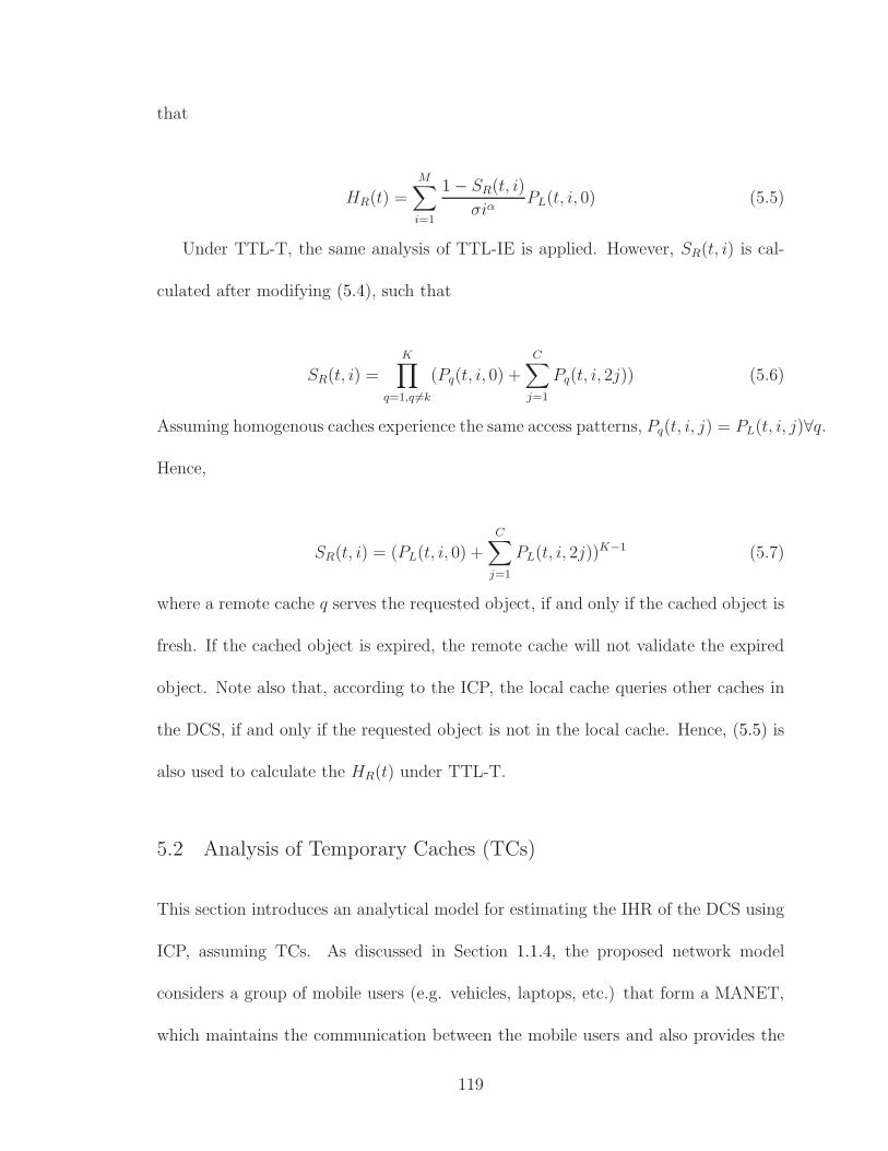
that
HR(t) =
M∑
i=1
1 − SR(t, i)
σiαPL(t, i, 0) (5.5)
Under TTL-T, the same analysis of TTL-IE is applied. However, SR(t, i) is cal-
culated after modifying (5.4), such that
SR(t, i) =
K∏
q=1,q 6=k
(Pq(t, i, 0) +
C∑
j=1
Pq(t, i, 2j)) (5.6)
Assuming homogenous caches experience the same access patterns, Pq(t, i, j) = PL(t, i, j)∀q.
Hence,
SR(t, i) = (PL(t, i, 0) +
C∑
j=1
PL(t, i, 2j))K−1 (5.7)
where a remote cache q serves the requested object, if and only if the cached object is
fresh. If the cached object is expired, the remote cache will not validate the expired
object. Note also that, according to the ICP, the local cache queries other caches in
the DCS, if and only if the requested object is not in the local cache. Hence, (5.5) is
also used to calculate the HR(t) under TTL-T.
5.2 Analysis of Temporary Caches (TCs)
This section introduces an analytical model for estimating the IHR of the DCS using
ICP, assuming TCs. As discussed in Section 1.1.4, the proposed network model
considers a group of mobile users (e.g. vehicles, laptops, etc.) that form a MANET,
which maintains the communication between the mobile users and also provides the
119

users with Internet connections. As illustrated in the VANET example in Fig. 1.7,
the proposed DCS assumes that there are some mobile users that have extra power
and cache storage to host TCs.
In the proposed DCS, the TCs cooperate with each other to serve mobile users
in the MANET, which improves the user’s perceived latency, reduces the load on
the infrastructure, and improves the network capacity. This is particularly useful in
periods of high load where a dense population is interested in accessing the same
objects. For example, during a sporting event or a concert where users are accessing
the same highlight footage at slightly different times, a small number of objects are
heavily requested by many users over a short time-span. In this scenario, the proposed
DCS prevents users from overwhelming the limited infrastructure bandwidth and
allows more users to simultaneously access the requested objects, as shown in Fig. 5.1.
The DCS with TCs follows the same network model and assumptions described in
Section 4.4.1. However, unlike the HCS, the proposed DCS consists of multiple TCs
in a single MANET. Fig. 5.2 shows the proposed DCS where each TC is associated
with a group of users who query that TC (local TC), rather than the access point.
Like the HCS, when a TC disconnects from the DCS, its users will be automatically
associated with the closest available TC in the MANET. When a new TC joins the
DCS, nearby users will automatically be associated with this new TC.
As discussed in Section 1.1.4, the user’s request is satisfied from the local TC,
if the TC has the requested object. Otherwise, the local TC will query the other
TCs (remote TCs) in the DCS for that object. If the object cannot be found in any
TC (remote TC) in the DCS, the TC downloads the requested object from the OS
120

Access Blocked
Access succeeded
Macrocell
Macrocell
Base station
MANET
User caches
the object
P2P Access
Access succeeded
Macrocell
Macrocell
Base station
User caches
the object Access succeeded
Figure 5.1: Network topology for temporary caches in the DCS.
via an infrastructure access point and forwards the object to the requesting user (or
the access point just forwards the object to the user and its TC). It is important to
note that the DCS adopts ICP where it is assumed that the remote TC serves a user
through the user’s local TC, which will store the requested object for future requests.
This constraint is relaxed in ICP-COCO, where the local TC does not cache objects
that are served by the remote TCs. Hence, the TC may only cache those objects
that are served by the OS, as shown in Fig 5.3. In Section 5.3, the steady state
performances of ICP and ICP-COCO will be evaluated.
For DCS using ICP, in order to estimate the local IHR of a TC, HL(t), the
121

Access
pointTC
online
TC
online
MANET
TC
offline
Access
pointTC
online
user served
by a TC
Figure 5.2: The proposed distributed TCs network model.
analysis introduced in Section 4.4 for the HCS with temporary leaf caches (TLCs)
can be used, under TTL-IE or TTL-T. Note that, similar to the analysis introduced in
Section 4.4, the TCs population is modeled as a birth-death process, with an arrival
rate that equals λu and a departure rate that equals µu.
However, in order to calculate the DCS remote IHR, HR(t), the analysis has to
account for the fact that the remote hit occurs when any remote TC in the DCS has
the requested object. Thus, the remote IHR, HR(t), is calculated using the analysis
122

(1) user
requests an
object
(3) Remote TC
forwards the object
to the user through
the local TC
(2) Local TC
does not have
the object
(4) ICP
Local TC caches the
object
Remote TC has
the object
(5) user receives the
requested object
(4) ICP-COCO
Local TC forwards the
object. The TC does not
cache the object
Access
point
Figure 5.3: The proposed DCS: ICP vs. ICP-COCO.
introduced in Section 5.1 for the DCS with FCs. Hence, under NEM and TTL-
IE, SR(t, i) is calculated using (5.4), whereas, under TTL-T, SR(t, i) is calculated
using (5.7), assuming homogenous TCs that experience the same access patterns.
5.3 Steady State Evaluation of the Proposed DCS
Similar to the evaluation for the HCS in Section 4.5, the workload generator is used to
generate 30 workload profiles that statistically conform with the mathematical models
adopted in this chapter. Each workload profile consists of a sequence of requests. Each
request in the generated workload includes requested object id, object expiry time,
requesting TC id, and the identities of the TCs that are currently connected to the
DCS. The simulator is used to calculate the local and remote SSHR for each cache
in the DCS. The final simulated SSHR is then determined by averaging the SSHR
for all the simulated profiles. The final simulated SSAHD is calculated using the
simulated SSHR values in (4.1). Note that only the steady state performance of the
DCS is evaluated in this section, while the robustness of the proposed DCS under a
non-stationary access pattern will be considered in future work.
123

For FCs and TCs, it is assumed that each cache has the same capacity, C, and the
same hop distances to the OS, DO = 10. The hop distance between any two caches
in the DCS is also constant and is equal DR = 2, and the hop distance to the local
cache is DL = 0.
The SSAHD is evaluated assuming that all the objects have the same expiry rate
µe (i.e. µe = µ(i) ∀i). Analysis and simulation factors and their levels are summarized
in Table 5.1. Note that the levels presented in Table 5.1 only aim at illustrating the
concepts introduced in this chapter and do not mimic any realistic workload.
Table 5.1: DCS: evaluation factors and levels.
Factor Symbol ValueNumber of objects M 1000Number of Caches K 10
Zipf Slope α 0.8 [14]Request Rate β 1000 request/hr
Cache Capacity C 10-50 ObjectsObject Expire Rate µe 1, 10 object/hr
Also, for the DCS with TCs, this section follows the TCs population model in
Section 4.5.4, where λu = 10 and µu = 11 and the total request rate in steady state
is β = 1000 requests/hour.
In the following, Section 5.3.1 presents the evaluation results for the DCS using
ICP, assuming FCs or TCs. Then, Section 5.3.2 discusses the evaluation results for
the DCS using ICP-COCO, assuming FCs or TCs. In all the plots in the follow-
ing sections, the data points are generated using simulation and the solid lines are
generated using analysis.
124

5.3.1 Evaluation of ICP
Figs. 5.4, 5.5, and 5.6 show the excellent match between analytical and simulation
results of ICP at different values of C, µe, η for FCs or TCs.
10 30 500
10
20
30
40
50
60
Cache Capacity
SS
HR
TTL−IE RemoteTTL−IE Localη=0.2 Remoteη=0.2 Localη=0.8 Remoteη=0.8 Local
10 30 502
3
4
5
6
7
8
9
10
Cache CapacityS
SA
HD
TTL−IETTL−T η=0.2TTL−T η=0.8
Figure 5.4: SSHR (in percent) and SSAHD of the DCS with FCs, using ICP underTTL-IE or TTL-T, where µe = 1.
10 30 500
10
20
30
40
50
Cache Capacity
SS
HR
TTL−IE RemoteTTL−IE Localη=0.2 Remoteη=0.2 Localη=0.8 Remoteη=0.8 Local
10 30 505
6
7
8
9
10
Cache Capacity
SS
AH
D
TTL−IETTL−T η=0.2TTL−T η=0.8
Figure 5.5: SSHR (in percent) and SSAHD of the DCS with TCs, using ICP underTTL-IE, where µe = 1.
Fig. 5.4 shows that when µe = 1, TTL-IE outperforms TTL-T in terms of the
SSAHD, assuming FCs. Fig. 5.4 shows that when η = 0.2, TTL-IE and TTL-T have
125

10 30 500
10
20
30
40
50
Cache Capacity
SS
HR
TTL−IE RemoteTTL−IE Localη=0.2 Remoteη=0.2 Localη=0.8 Remoteη=0.8 Local
10 30 505
6
7
8
9
10
Cache Capacity
SS
AH
D
TTL−IETTL−T η=0.2TTL−T η=0.8
Figure 5.6: SSHR (in percent) and SSAHD of the DCS with FCs, using ICP underTTL-IE or TTL-T, where µe = 10.
similar local SSHR. Under TTL-T, the SSHR of a local cache decreases as η increases.
This is consistent with the result for the SCS in Section 3.9. Also, Fig. 5.4 shows
that TTL-IE yields a better remote SSHR than TTL-T. This is because ICP does not
allow remote requests to validate the expired objects. Hence, since the remote hit
occurs only if the requested object is fresh, TTL-IE that allows only fresh object to
linger in remote caches yields more remote hits. These results for FCs are also true
for TCs, as shown in Fig. 5.5. However, for TCs, the SSAHD increases as a result of
TCs disconnections.
Fig. 5.6 shows that when µe = 10, assuming FCs, TTL-T outperforms TTL-IE in
terms of SSAHD if η is small (e.g. 0.2) and C is large (e.g. 50). Fig. 5.6 shows that
TTL-T achieves a better local SSHR than TTL-IE, regardless of the value of η. The
superiority of TTL-T in terms of local SSHR increases as C increases. Again, this
is consistent with the results in Section 3.9. However, Fig. 5.6 shows that TTL-IE
achieves a better remote SSHR than TTL-T. Since the objects in remote caches are
126

more likely to be expired as µe increases, TTL-T allows remote caches to be polluted
(from the local cache perspective) by more expired objects that cannot be validated.
Moreover, the remote SSHR under TTL-T greatly degrades as C increases. This is
because as C increases, the local cache keeps more expired objects that are validated
directly from the OS, which reduces the request rate for the remote caches. Moreover,
as C increases, the local cache hits increase, which also reduces the request rate for
the remote caches. Fig. 5.6 shows that when η = 0.8, as C increases, the local
SSHR increases slowly, while the remote SSHR decreases quickly. This results in
an interesting behavior for TTL-T with η = 0.8, where the lowest SSAHD of 7.7 is
achieved when C = 20, while the SSAHD increases as C increases (e.g. the SSAHD
is 8 when C = 50), as illustrated in Fig. 5.6.
5.3.2 Evaluation of ICP-COCO
Fig. 5.7 shows that when µe = 1, ICP-COCO under TTL-IE outperforms ICP-COCO
under TTL-T in terms of SSAHD, assuming FCs. However, unlike ICP, ICP-COCO
under TTL-T achieves a better local SSHR than ICP-COCO under TTL-IE. Since
the cache under TTL-T does not validate an expired object due to a remote request,
ICP-COCO under TTL-T allows multiple copies of the same object to be cached at
different locations in the DCS. This redundancy plays a key role in improving the
local SSHR, since it increases the average lifetime of an object within the DCS. On
the other hand, TTL-IE degrades the local SSHR, since it allows only one copy to be
cached at a time. To better explain this point, let N(i) denote the number of copies
of object i that are currently cached. Under TTL-T, the average lifetime of a cached
127

object i in the DCS, L(i), is a random variable that is equivalent to the maximum of
N(i) exponential random variables that have the same rate µe. In this case, L(i) can
be calculated using (5.8) [153].
L(i) =
N(i)∑
x=1
1/xµe (5.8)
According to (5.8), for TTL-IE (i.e. N(i) ≤ 1), the average lifetime of 1/µe is
obtained. Thus, TTL-T outperforms TTL-IE, since L(i) is proportional to the number
of object copies, N(i).
10 30 500
20
40
60
80
100
Cache Capacity
SS
HR
TTL−IE RemoteTTL−IE Localη=0.2 Remoteη=0.2 Localη=0.8 Remoteη=0.8 Local
10 30 502
3
4
5
6
7
8
9
10
Cache Capacity
SS
AH
D
TTL−IETTL−T η=0.2TTL−T η=0.8
Figure 5.7: SSHR (in percent) and SSAHD of the DCS with FCs, using ICP-COCOunder TTL-IE or TTL-T, where µe = 1.
Furthermore, Fig. 5.7 shows that, like ICP, ICP-COCO under TTL-IE achieves a
better remote SSHR than ICP-COCO under TTL-T, when µe = 1. The first reason is
that ICP-COCO under TTL-IE allows only a single copy of each object to be cached
at a time. Hence, TTL-IE uses the available cache capacities on the remote caches
more effectively than TTL-T. Second, ICP-COCO under TTL-T wastes the cache
capacity of remote caches by allowing expired objects to be stored, as discussed in
128

Section 5.3.2.
The results for FCs in Fig. 5.7 are also true for TCs, as shown in Fig. 5.8 where
TTL-IE achieves a better remote SSHR and a better SSAHD, while TTL-T achieves
a better local SSHR. However, for TCs, the local SSHR of TTL-T becomes closer to
the SSHR of TTL-IE, since the advantage of allowing multiple copies under TTL-
T vanishes due to TCs disconnections. Also, for TCs, TTL-IE and TTL-T achieve
similar remote SSHRs. This is because under TTL-IE, the DCS loses single copies
of popular objects quickly due to TCs disconnections, while allowing multiple copies
under TTL-T provides a backup for the loss of popular objects.
10 30 500
10
20
30
40
50
60
Cache Capacity
SS
HR
TTL−IE RemoteTTL−IE Localη=0.2 Remoteη=0.2 Localη=0.8 Remoteη=0.8 Local
10 30 505
6
7
8
9
10
Cache Capacity
SS
AH
D
TTL−IETTL−T η=0.2TTL−T η=0.8
Figure 5.8: SSHR (in percent) and SSAHD of the DCS with TCs, using ICP-COCOunder TTL-IE, where µe = 1.
Fig. 5.9 shows that when µe = 10, ICP-COCO under TTL-T outperforms ICP-
COCO under TTL-IE in terms of SSAHD if η is small (e.g. 0.2) and C is large,
assuming FCs. This is similar to the results obtained for ICP in Fig. 5.6. However,
note that the SSAHD of TTL-T when η = 0.8 becomes closer to the SSAHD of TTL-
IE when ICP-COCO is used. This is because of the rapid increase in the local SSHR
129

of ICP-COCO under TTL-T. Furthermore, like ICP, TTL-T with η = 0.8 achieves
the lowest SSAHD of 7.85 at C = 30. Then, the SSAHD increases as C increases
(e.g. at C = 50, the SSAHD is 8).
10 30 500
10
20
30
40
50
Cache Capacity
SS
HR
TTL−IE RemoteTTL−IE Localη=0.2 Remoteη=0.2 Localη=0.8 Remoteη=0.8 Local
10 30 505
6
7
8
9
10
Cache CapacityS
SA
HD
TTL−IETTL−T η=0.2TTL−T η=0.8
Figure 5.9: SSHR (in percent) and SSAHD of the DCS with FCs, using ICP-COCOunder TTL-IE or TTL-T, where µe = 10.
Note that, compared to ICP, ICP-COCO improves the SSAHD of the DCS with
FCs, if µe = 0 (i.e. under NEM). Under NEM, ICP-COCO uses the cache capacity
more efficiently by allowing at most one copy of an object to be stored in the DCS.
However, this is not true under TTL-IE, since the multiple copies allowed by ICP
increase the average object lifetime in the network, according to (5.8). Table 5.2
illustrates the SSAHD of ICP-COCO and ICP under NEM and TTL-IE, when µe = 1.
Furthermore, the multiple copies provide backup for the loss of the popular objects
in case of DCS with TCs. Hence, ICP achieves a better SSAHD than ICP-COCO
under NEM as well as TTL-IE, as shown in Table 5.3.
130

Table 5.2: SSAHD of ICP and ICP-COCO under NEM and TTL-IE, where µe = 1,assuming FCs.
C NEM TTL-IEICP ICP-COCO ICP ICP-COCO
30 5.37 5.2 5.42 5.4140 4.84 4.58 4.91 4.9850 4.40 3.98 4.48 4.86
Table 5.3: SSAHD of ICP and ICP-COCO under NEM and TTL-IE, where µe = 1,assuming TCs.
C NEM TTL-IEICP ICP-COCO ICP ICP-COCO
30 6.42 6.58 6.48 6.7940 6.06 6.33 6.18 6.6550 5.79 6.15 6.0 6.49
5.4 Summary
In this chapter, the steady state performance of the DCS using ICP and ICP-COCO
was evaluated. The results in this section were as follows:
• For both ICP and ICP-COCO, TTL-IE yields a better SSAHD than TTL-T,
when µe is moderate (e.g. 1 per hour). This is true for FCs as well as TCs. However,
for FCs, TTL-T yields a better SSAHD than TTL-IE when µe is high (e.g. 10 per
hour) and the validation factor, η, is small.
• For both ICP and ICP-COCO, TTL-IE yields a better remote SSHR than TTL-
T. This is because a remote hit only occurs if the requested object in the remote
cache is fresh. Hence, with respect to a local cache, TTL-T allows remote caches to
be polluted by expired objects that cannot be validated. This greatly degrades the
131
remote SSHR under TTL-T, especially when µe is high.
• For both ICP and ICP-COCO under TTL-T, when η = 0.8 and µe = 10, as C
increases, the local SSHR increases, while the remote SSHR decreases rapidly. This
results in an interesting behavior where the SSAHD increases as a function of C.
• For ICP-COCO, TTL-T improves the local SSHR assuming FCs or TCs. This
is true especially for FCs when µe is high (e.g. 10 per hour), which allows TTL-T to
achieve a better SSAHD than TTL-IE when η is small.
• For FCs under NEM, ICP-COCO outperforms ICP since ICP-COCO utilizes
the cache capacities more efficiently by allowing only one copy of each object to be
cached at a time. However, for TCs, or under TTL-IE, ICP outperforms ICP-COCO
since allowing multiple copies plays a crucial role either to backup the loss of popular
objects due to disconnections, in case of TCs, or due to expiry, in case of TTL-IE.
132

Chapter 6
Conclusions and Future Work
In this chapter, the conclusions of this dissertation are presented in Section 6.1. Then,
the future work is discussed in Section 6.2.
6.1 Conclusions
Caching Web objects close to end users allows users’ requests to be satisfied from
a nearby Web cache rather than a faraway origin server (OS). Cache hits improve
the user’s perceived latency, reduce the load on the OS, and achieve bandwidth sav-
ings over costly Internet links. In this dissertation, three Web cache systems are
considered: a single cache system (SCS), a hierarchical cache system (HCS), and a
distributed cache system (DCS).
In Chapter 3, an analytical model for estimating the instantaneous hit ratio (IHR)
of the SCS was introduced. Estimating the IHR is important for any application where
the number of objects, object popularity, and/or the caching resources themselves
are subject to change. Consider a scenario where objects experience only short-term
popularity, such as a group of users watching sports highlights or accessing vehicular
traffic information. Here, it is important for a cache to reach maximum performance
quickly before the popularity of the cached objects starts to drop. Moreover, a ve-
hicular or mobile network may store cached objects on mobile devices. In this case,
it is also important for the cache to reach a high hit ratio quickly before the mobile
133

device that is hosting the cache disconnects from the network.
Chapter 3 was focused on evaluating how the cache hit ratio evolves as a function
of time in two cases. The first case assumed a stationary access pattern where the
number of objects and the object popularity are fixed throughout the evaluation
interval. In this case, the IHR was evaluated in the transient period starting from an
empty cache. The second case adopted more realistic assumptions by assuming that
the number of objects increases periodically (i.e. non-stationary access pattern). It
was assumed that the most recently generated objects become the most popular ones
(news headlines, for example). Hence, the popularity of the formerly cached objects
decreases every time new objects are generated. In this case, the cache may not reach
the steady state and the only way to quantify the hit ratio experienced by users is to
calculate the IHR.
Moreover, the SCS analysis in Chapter 3 accommodates either an infinite or a
finite cache capacity. For the finite case, the cache applies a replacement policy to
decide which objects to keep. The proposed analysis introduced a solution for two
replacement policies: LRU and FIFO. Furthermore, the proposed analysis considered
a typical TTL mechanism (i.e. TTL-T), whereby the request for an expired cached
object results in sending a HTTP conditional GET request to the OS. In this case,
the replacement policy does not distinguish expired objects from the fresh ones. This
was compared to a second TTL implementation where cached objects are ejected
immediately once they expire (i.e. TTL-IE). In this second case, the replacement
policy is applied only to fresh objects, since expired objects do not exist in the cache.
Also, the case where objects do not expire is considered (i.e. NEM).
134

Furthermore, Chapter 3 introduced a new replacement policy, called frequency-
based-FIFO (FB-FIFO). FB-FIFO improves the IHR of FIFO by creating a variable-
sized protected cache segment for objects that are not effectively one-timers. The
results showed that the replacement policy using the two implementations for TTL
(i.e. TTL-T and TTL-IE) yields different IHRs, especially for large caches. Under
TTL-IE or TTL-T, the results showed that FB-FIFO outperforms the steady state
hit ratio (SSHR) of FIFO and LRU.
The results in Chapter 3 illustrated that the considered replacement policies have
very different transient performance, whether the popularity of cached objects is fixed
or not. This makes the proposed analysis valuable when considering scenarios like
changing popularity or mobile caching. Under TTL-IE, assuming a stationary access
pattern, the results showed that the hit ratio reaches a steady state within a period
that depends on cache capacity, object expiry rate, and request rate. In this case,
the results showed that FB-FIFO outperforms FIFO and LRU in the steady state,
especially for small cache capacities. On the other hand, these results change when the
OS periodically generates new popular objects. Furthermore, the results showed that
when the OS generates new popular objects periodically, the users may experience
different hit ratios when they initiate requests at different times. In this case, the hit
ratio experienced by these users can only be quantified by calculating the IHR.
In Chapter 4, an analytical model for estimating the instantaneous average hit
distance (IAHD) of a two-level HCS was proposed. The proposed analytical model
considers LCE sharing protocol under NEM, TTL-IE, and TTL-T. Also, the design
and analysis of a new hierarchical sharing protocol, called PCO, were introduced.
135

Simulations were used to validate the analytical results for LCE and PCO and to
compare them with LCD.
The results in Chapter 4 showed that the steady state performance of the con-
sidered sharing protocols depends on the object expiry rate and the adopted TTL
implementation. Assuming NEM, the results showed that PCO achieves the best
steady state average hit distance (SSAHD) followed by LCD then LCE. This is espe-
cially true when the root cache is large. The results showed that this is also true under
TTL-T. However, under TTL-IE, the SSAHDs of PCO and LCD degrade rapidly as
the object expiry rate increases. Also, under NEM, the results showed the superiority
of PCO for the HCS with temporary leaf caches (TLCs) that suffer from frequent
disconnects.
Moreover, in Chapter 4, the robustness of the considered sharing protocols was
evaluated assuming a non-stationary access pattern. Assuming NEM, the results
showed that PCO is more robust than LCD when new popular objects are generated,
especially when the root cache is small. However, when the root cache capacity is
large, and as the number of newly generated objects increases, LCD and LCE become
more robust than PCO, at the expense of the SSAHD.
In Chapter 5, an analytical model for estimating the IAHD of a DCS using ICP
was proposed. The proposed analysis for the DCS considered LRU caches under
NEM, TTL-IE, and TTL-T. Moreover, a modified version of the ICP, called ICP-
COCO, where the object that is served by a remote cache is not locally cached, was
evaluated using simulations. ICP-COCO under NEM or TTL-IE allows only one copy
of the same object to exist in the DCS at a time, while this is not true for ICP-COCO
136

under TTL-T.
The results in Chapter 5 showed that, for both ICP and ICP-COCO, TTL-IE
yields a better SSAHD than TTL-T, when the object expiry rate, µe, is moderate
(e.g. 1 per hour). This is true for a DCS with either fixed caches (FCs), or temporary
caches (TCs). However, for FCs, TTL-T yields a better SSAHD than TTL-IE when
µe is high (e.g. 10 per hour) and the validation factor, η, is small. Furthermore, the
results for FCs showed an interesting behavior where the SSAHD increases as the
cache capacity increases. This occurs for both ICP and ICP-COCO under TTL-T,
when the validation factor, η = 0.8, and the object expiry rate, µe = 10. Moreover,
the results also showed that, for FCs under NEM, ICP-COCO outperforms ICP.
However, this is not true for TCs, or under TTL-IE.
6.2 Future work
The findings in this dissertation are valid under the independent reference model
(IRM), which is widely used to develop tractable analytical cache models. However,
the IRM might not accurately model empirical traces that have varying degrees of
temporal correlation between object requests, as discussed in Section 2.3. Thus,
an interesting extension of the proposed model would be to incorporate short term
popularity [14,62,109]. For example, the LRU stack in [14] maintains an ordered list of
documents based on recency of access, which can be modeled using the proposed LRU
Markov chain. In a static LRU stack, the probability of referencing is associated with
the stack position, whereas in a dynamic LRU stack, the probability of referencing
137

depends on the object identity as well as the stack position [106].
Furthermore, in the proposed LRU Markov chain, the probability that an object
is requested depends entirely on the object identity. Therefore, the main difference
between the LRU stack models and the proposed LRU Markov chain is that in LRU
stack, the request rate of object i, λ(i), is a function of the current state j. For
example, let λ(i, j) denote the request rate of object i that is currently occupying
state j in the LRU stack. Then, λ(i, j) can be calculated as λ(i, j) = βf(i, j), where
f(i, j) is the probability that object i that is currently in state j will be requested.
Note that in the proposed LRU Markov chain f(i, j) = 1/(σiα), which is independent
of j, as discussed in Section 3.1.
For the HCS, four main issues will be considered in future work. First, it is
important to evaluate the considered sharing protocols using more than two cache
levels. This can be done based on the concepts proposed for two-level hierarchy in
Chapter 4. Second, individual caches at different levels may follow different consis-
tency models and it would be interesting to evaluate LCE, PCO, and LCD in this
case. Also, evaluating the HCS, with each level running a different replacement policy
can be done using the proposed analysis in Chapter 4. Third, the proposed analysis
in Chapter 4 for PCO under TTL-IE can also be extended for PCO under TTL-T.
Finally, incorporating more realistic connectivity model for TLCs into the proposed
simulation and analysis remains an interesting point. It will be interesting to eval-
uate the considered sharing protocols using more realistic mobility models, such as
Random Waypoint and Random Walk [154,155,156]. Also, comparing the analytical
results to trace-based simulations, which use real traces, will be considered.
138

For the DCS, the steady state evaluation was presented in Chapter 5, while evalu-
ating the robustness of the proposed DCS under a non-stationary access pattern will
be considered in future work. Also, comparing the IAHDs of the proposed HCS and
DCS will be considered. Moreover, the proposed analysis for the DCS and HCS will
be extended for a two-level hybrid cache system, where a root cache at the second
level resolves the misses of the DCS at the first level.
Furthermore, for the DCS, it is important to extend the proposed analysis for het-
erogenous caches that use different consistency mechanisms and replacement policies,
and experience different access patterns. Also, I believe that the proposed analytical
model can be extended for other DCS sharing protocols, such as cache array routing
protocol (CARP) [45].
Furthermore, evaluating the effect of relaxing some ICP assumptions will be in-
teresting, for example, relaxing the assumption that the local cache is not affected by
the remote hits. This is called dependent-LRU, as discussed in Section 2.6.2. Fig. 6.1
shows the Markov chain that can be used to calculate the local hit of cache k, Hzk(t),
under TTL-IE, assuming dependent-LRU. Unlike the Markov chain shown in Fig. 3.8
for SCS, the rate at which an object i moves from a cache-fresh state (CFS) to state
Ck in Fig. 6.1, ωk(t, i), depends on the remote access pattern, such that
ωk(t, i) = λk(i) +
K∑
q=1,q 6=k
λq(i)P∗q (t, i, 0) (6.1)
where a cache k, unlike the other caches in the DCS, works under dependent-LRU.
Note that P ∗q (t, i, 0)∀q has to be calculated first in order to find Hz
k(t). On the other
139
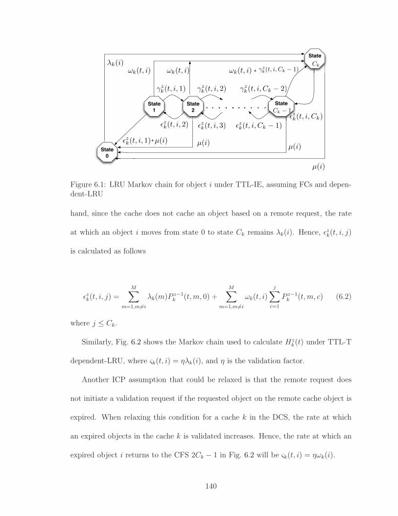
State
0
State
1
State
2
State
State
+
+
λk(i)
µ(i) µ(i)µ(i)
µ(i)
γz
k(t, i, 1) γ
z
k(t, i, 2) γ
z
k(t, i, Ck − 2)
γz
k(t, i, Ck − 1)
ǫz
k(t, i, 2)
ǫz
k(t, i, 1)
ǫz
k(t, i, 3) ǫ
z
k(t, i, Ck − 1)
ǫz
k(t, i, Ck)
Ck
Ck − 1
ωk(t, i) ωk(t, i) ωk(t, i)
Figure 6.1: LRU Markov chain for object i under TTL-IE, assuming FCs and depen-dent-LRU
hand, since the cache does not cache an object based on a remote request, the rate
at which an object i moves from state 0 to state Ck remains λk(i). Hence, ǫzk(t, i, j)
is calculated as follows
ǫzk(t, i, j) =
M∑
m=1,m6=i
λk(m)P z−1k (t, m, 0) +
M∑
m=1,m6=i
ωk(t, i)
j∑
c=1
P z−1k (t, m, c) (6.2)
where j ≤ Ck.
Similarly, Fig. 6.2 shows the Markov chain used to calculate Hzk(t) under TTL-T
dependent-LRU, where ςk(t, i) = ηλk(i), and η is the validation factor.
Another ICP assumption that could be relaxed is that the remote request does
not initiate a validation request if the requested object on the remote cache object is
expired. When relaxing this condition for a cache k in the DCS, the rate at which
an expired objects in the cache k is validated increases. Hence, the rate at which an
expired object i returns to the CFS 2Ck − 1 in Fig. 6.2 will be ςk(t, i) = ηωk(i).
140
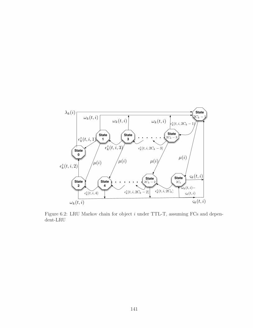
State
0
State
1
State
3
State
State
State
2
State
4
2Ck − 3
State
2Ck − 2
State
2Ck
λk(i)
ǫz
k(t, i, 2)
ǫz
k(t, i, 1)
µ(i) µ(i) µ(i)µ(i)
ǫz
k(t, i, 3)
ǫz
k(t, i, 2Ck − 1)
2Ck − 1
ǫz
k(t, i, 2Ck − 3)
ςk(t, i)
ςk(t, i)
ǫz
k(t, i, 2Ck)
ǫz
k(t, i, 2Ck − 2)
ǫz
k(t, i, 4)
ωk(t, i)ωk(t, i) ωk(t, i)
ωk(t, i)
ωk(t, i)−
ςk(t, i)
Figure 6.2: LRU Markov chain for object i under TTL-T, assuming FCs and depen-dent-LRU
141

Appendix A
Convergence of the Proposed Analysis
This appendix discusses the convergence of the proposed contraction mapping analysis
introduced in Chapter 3. First, a brief background for the contraction mapping theory
(CMT) is presented in Section A.1. Then, the convergence of FIFO analysis under
NEM is discussed in Section A.2. The convergence of FIFO analysis under TTL-IE
and TTL-T is discussed in Section A.3. Finally, the convergence of LRU analysis
under NEM is discussed in Section A.4.
A.1 Contraction Mapping Theory (CMT)
The principle of contraction mapping, and the corresponding contraction mapping
theorems (CMTs), have proved extremely useful in the analysis of nonlinear dynam-
ical systems [32, 33, 34]. The most basic CMT in ℜ, which was published by Banach
in 1922, states that
Theorem 1 (Banach’s CMT in ℜ) [32]: Consider f : ℜ → ℜ is a continues
scalar-valued function such that: (1) For every x from the interval [a, b], its image
f(x) also belongs to the same interval [a, b], and (2) There exists a positive constant
c < 1, where |f(x) − f(y)| ≤ c|x − y|, ∀x, y ∈ [a, b], or |f ′(x)| ≤ c, ∀x ∈ (a, b). Then
f is called a contraction mapping over [a, b] and the equation x = f(x) has a unique
solution x∗ ∈ [a, b], and the iteration xz+1 = f(xz) converges to x∗, starting from any
142

point x0 ∈ [a, b].
The first condition in Theorem 1 guarantees the existence of the solution x∗ ∈
[a, b]. This can be explained using the intermediate value theorem, as follows. Since
f(a) ≥ a and f(b) ≤ b, we have f(b) − b ≤ 0 ≤ f(a) − a. The difference f(x) − x is
continuous, so by the intermediate value theorem 0 is a value of f(x∗) − x∗ for some
x∗ ∈ [a, b], and that x∗ is a fixed point of f [33]. The second condition in Theorem 1
guarantees the uniqueness of the fixed point (i.e. x∗ is the only fixed point in [a, b]),
and the converges to x∗ starting from any point x0 ∈ [a, b].
For example, y = cos(x) and y = x intersect once, as shown in Fig. A.1, which
means the cosine function has a unique fixed point in ℜ. From Fig. A.1, this fixed
point lies in [0, 1] [33].
Figure A.1: cos(x) is a contraction mapping [33].
To proof that cos(x) is a contraction mapping on [0, 1], first lets check cos(x) maps
[0, 1] to [0, 1]. Since cosine is decreasing on [0, 1] and cos(1) ≈ 0.54, cos([0, 1]) → [0, 1].
Second, it is difficult to find c < 1 such that |cos(x)− cos(y)| ≤ c|x−y|, ∀x, y ∈ [0, 1].
However, calculating |cos(t)′| = |sin(t)| over [0, 1] will give us a contraction constant,
c. Since sin(t) is increasing (monotonic increase function) on [0, 1], ∀t ∈ [0, 1] we
have |sin(t)| = sin(t) ≤ sin(1) ≈ 0.84147. Therefore |cos(x) − cos(y)| ≤ .8415|x −
143

y|, ∀x, y ∈ [0, 1] [33]. Thus, from Theorem,1, there is a unique solution of cos(x) =
x ∈ [0, 1] and it can be found by iterating the function cos(x) starting from any initial
point in [0, 1]. Table A.1 shows the contraction mapping iterations of cos(x) starting
from x0 = 1:
Table A.1: The contraction mapping of cos(x) [33].
z xz
0 11 0.5403023...
...18 0.739303819 0.738937720 0.739184321 0.7390182
Furthermore, in some situations, a function is not a contraction but an iterate
of it is. This turns out to suffice to get the conclusion of the contraction mapping
theorem for the original function, according to the following theorem.
Theorem 2 (Generalizations of Theorem 1) [33]: Consider f : ℜ → ℜ is
a continues scalar-valued function, such that some iterate f z : [a, b] → [a, b] is a
contraction, then f has a unique fixed point, x∗, which can be obtained by iteration of
f starting from any x0 ∈ [a, b].
For example, Fig. A.2 shows that y = ex and y = x intersect once, so ea = a for a
unique real number a. The function f(x) = ex is not a contraction on ℜ (for instance,
|f(−2) − f(0)| ≈ 6.38 > | − 2 − 0|), but its second iterate g(x) = f 2(x) = e−e−x
is a
contraction on ℜ. For some t between x and y, where |g′(t)| = |e−e−t
e−t| = e−(t+e−t) ≤
144

Figure A.2: ex is a contraction mapping [33].
e−1 (since t + e−t ≥ 1, ∀t ∈ ℜ). Hence f 2 has contraction constant 1/e ≈ .367 < 1.
From Theorem 2, the solution to e−a = a can be approximated by iteration of f
starting with any real number like the example in Table A.1 [33].
Moreover, for a vector-valued function, the Theorem 1 can be extended to ℜN as
follows:
Theorem 3 (CMT in ℜN) [34]: A function f: ℜN → ℜN is a contraction mapping
on a domain π ∈ ℜN , if (1) it maps π to itself, so f(u) ∈ π whenever u ∈ π, and (2)
there exists a constant 0 ≤ c < 1 such that ||g(u)− g(v)|| ≤ c||u− v||, ∀u,v ∈ π, or
if the Jacobian matrix norm1||f ′(u)|| < 1, ∀u ∈ π.
The Jacobian matrix of f ′(u), where u = [u1, u2, . . . , uN ], can be calculated us-
ing (A.1), and the the infinity norm of the matrix v = f ′(u) is given by ||v||∞ =
1Both 1 or ∞ norms can be used [34]
145

max1≤i≤N(|vi|).
f ′(u) =
∂f1
∂u1
∂f1
∂u2. . . ∂f1
∂ui. . . ∂f1
∂uN
∂f2
∂u1
∂f2
∂u2. . . ∂f2
∂Pi. . . ∂f2
∂uN
......
......
......
∂fN−1
∂u1
∂fN−1
∂u2. . . ∂fN−1
∂ui. . . ∂fN−1
∂uN
∂fN
∂u1
∂fN
∂u2. . . ∂fN
∂ui. . . ∂fN
∂uN
(A.1)
A.2 FIFO under NEM
In this section, the convergence of FIFO analysis under NEM is discussed. First,
Section A.2.1 discusses the convergence of FIFO analysis in the steady state, as-
suming uniform object popularity. Then, Section A.2.2 discusses the convergence of
FIFO analysis in the steady state, assuming Zipf-like object popularity. Section A.2.3
discusses the convergence of the FIFO analysis in the transient state.
A.2.1 Convergence in Steady State, Assuming Uniform Object Popularity
Markov chain balance equations can be used to show convergence for a scalar function
under the following assumptions:
(S.1) The cache is in steady state (i.e. t → ∞). Thus, P z(i, 0) = limt→∞ P z(t, i, 0)
∀ i ∈ [1, M ].
(S.2) The objects are requested with equal probability (i.e. α = 0). Thus,
P z(0) = P z(i, 0) ∀ i ∈ [1, M ].
Also, in order to simplify the use of the balance equations, NEM is assumed, such
146

that:
(S.3) Objects do not expire (i.e. µ(i) = 0 ∀ i).
According to Theorem 1 in Section A.1, f : (0, 1] → (0, 1] is a contraction mapping
and converges to a unique fixed point, P ∗(0), starting from any initial point, P 0(0) ∈
(0, 1], if:
(C.1) f : (0, 1] → (0, 1] is a continuous function.
(C.2) | f ′(P (0)) | < 1 ∀P (0) ∈ (0, 1]. Also, (C.2) can be generalized to:
(C.2.1) | g′(P (0)) | < 1 ∀P (0) ∈ (0, 1], g(P (0)) = f(f(P (0))).
For FIFO, according to (3.15) and using (S.2), we have:
ǫz(i, j) = (β − λ)P z−1(0) (A.2)
Using (A.2) and (S.3) to solve the balance equations and calculate the limiting prob-
ability P z(0), we have:
P z(0) =(M − 1)P z−1(0)
(M − 1)P z−1(0) + C=
ρP z−1(0)
ρP z−1(0) + 1
where ρ ≈ M/C > 1, for large M , or equivalently
f(P (0)) =ρP (0)
ρP (0) + 1(A.3)
From (A.3), f(P (0)) satisfies (C.1). Also,
f ′(P (0)) =ρ
[ρP (0) + 1]2(A.4)
147

f ′(f(P (0))) =ρ2
[ρ2P (0) + ρP (0) + 1]2(A.5)
Note that the analysis in Section 3.4.1 calculates P 1(0) assuming that all objects
are not in cache (i.e., P 0(0) = 1). Hence, the analysis initializes P (0) = 1 then P (0)
decreases iteratively until reaching the fixed point P ∗(0) = ρ−1ρ
, according to (A.3).
Therefore, it is suffice to proof that the maximum slope of f(P0), which occurs at the
fixed point P ∗(0), is less than 1 (i.e., |f ′(P ∗(0))| < 1, or |f ′(f(P ∗(0)))| < 1). From
(A.4), f(P (0)) satisfies (C.2) ∀ P (0) ∈ [P ∗(0), 1] even for very small ρ. The example
in Fig. A.3 shows that when ρ = 2, the analysis converges to P ∗(0) = ρ−1ρ
= 0.5 and
f ′(P ∗(0)) = f ′(0.5) = 0.5 < 1. Note that in Fig. A.3 two functions are plotted:
• Y = P (0)
• Y = f1(P (0)), where the function f1 is calculated using the exact expressions
provided in Section 3.4.1
0 0.1 0.2 0.3 0.4 0.5 0.6 0.7 0.8 0.9 1.00
0.2
0.4
0.6
0.8
1
P0
Y = P0
Y=f1(P
0)
Figure A.3: FIFO iterative analysis, where M = 100 and C = 50.
Another example in Fig. A.4 shows that the analysis converges to P ∗(0) = ρ−1ρ
=
148

0.9 from the right, under the assumption that P (0) is initialized to 1. Thus, the
output steady state hit ratio is C/M = 10%, as illustrated in Table A.2.
0 0.1 0.2 0.3 0.4 0.5 0.6 0.7 0.8 0.9 1.00
0.2
0.4
0.6
0.8
1
P0
Y = P0
Y=f1(P
0)
Figure A.4: FIFO iterative analysis, where M = 1000 and C = 100.
Table A.2: FIFO iterative analysis, where M = 1000 and C = 100.
Iteration z P z(0) f1(Pz(0)) Hit ratio
1 1 0.90901 9.09918 %2 0.90901 0.90080 9.91965 %3 0.90080 0.89999 10.0009 %4 0.89999 0.89999 10.0009 %
Furthermore, according to (A.5), the analysis converges to P ∗(0) = ρ−1ρ
when ρ is
small, even when P (0) is initialized by a small value that is bigger than zero (e.g. for
ρ = 10 and P (0) = 0.1, f ′(f(0.1)) = 0.694 < 1).
A.2.2 Convergence in Steady State, Assuming Zipf-like Object Popularity
According to (3.15), we have
149

ǫz(i) =M
∑
m=1,m6=i
λ(m)P z−1(m, 0) (A.6)
Since the Markov chain is at equilibrium, we have
λ(i)P z(i, 0) = ǫz(i)P z(i, 1)
ǫz(i)P z(i, 1) = ǫz(i)P z(i, 2)
ǫz(i)P z(i, 2) = ǫz(i)P z(i, 3)
...
ǫz(i)P z(i, j) = ǫz(i)P z(i, j + 1)
...
ǫz(i)P z(i, C − 1) = λ(i)P z(i, C)
ǫz(i)P z(i, C) = λ(i)P z(i, 0)
Thus,
P z(i, C) = P z(i, C − 1) = . . . = P z(i, 1) =λ(i)
ǫz(i)P z(i, 0) (A.7)
From (A.7), and since∑C
c=0 P z(i, c) = 1, we have
150

1 = P z(i, 0) + CP z(i, C)
1 = P z(i, 0) +Cλ(i)
ǫzi
P z(i, 0)
1 = P z(i, 0)
[
1 +Cλ(i)
ǫz(i)
]
P z(i, 0) =ǫz(i)
Cλ(i) + ǫz(i)(A.8)
From (A.8), and using (A.6), we have
P z(i, 0) =
∑Mm=1,m6=i λ(m)P z−1(m, 0)
Cλ(i) +∑M
m=1,m6=i λ(m)P z−1(m, 0)(A.9)
Let vzi denote P z(i, 0) and v = [v1, v2, . . . , vM ]. Thus, f(v) = [f1, f2, . . . , fM ],
where fi =PM
m=1,m6=i λ(m)vz−1m
Cλ(i)+PM
m=1,m6=i λmvz−1m
, according to (A.9). Therefore,
f ′(v) =
0 ∂f1
∂v2. . . ∂f1
∂vi. . . ∂f1
∂vM
∂f2
∂v10 . . . ∂f2
∂vi. . . ∂f2
∂vM
......
......
......
∂fM−1
∂v1
∂fM−1
∂v2. . . ∂fM−1
∂vi. . . ∂fM−1
∂vM
∂fM
∂v1
∂fM
∂v2. . . ∂fM
∂vi. . . 0
where ∂fi
∂vi= 0. For x 6= i, we have
∂fi
∂vx=
∂
∂vx
∑
m λmvm
Cλ(i) +∑
m λmvm(A.10)
For w 6= x, we have
151

∂fi
∂vx=
∂
∂vx
λ(x)vx +∑
w λ(w)vw
Cλ(i) + λ(x)vx +∑
w λ(w)vw
=λ(x)(λ(x)vx + Cλ(i) +
∑
w λ(w)vw) − λ(x)(λ(x)vx +∑
w λ(w)vw)
(Cλ(i) + λ(x)vx +∑
w λ(w)vw)2
=Cλ(i)λ(x)
(Cλ(i) +∑
m λ(m)vm)2
=Cλ(i)λ(x)
(Cλ(i) + πi)2
where π(i) =∑M
m6=i λ(m)vm = β − λ(i). Thus, the sum of the ith row, yi, in f ′(v) is
yi =Cλ(i)
∑
m λ(m)
(Cλ(i) + π(i))2
=Cλ(i)(β − λ(i))
(Cλ(i) + π(i))2
=Cλ(i)β − Cλ(i)2
(Cλ(i) + π(i))2(A.11)
In order to calculate ||f ′(v)||∞ = max1≤i≤M (|yi|),∂yi
∂λ(i)has to be calculated first.
Since the miss rate of a single object is so small compared with the aggregate miss
rates of all M other objects, it’s reasonable to assume that π is constant ∀i. This will
allow us to calculate ∂yi
∂λ(i)by taking the derivative of (A.11) as follows
∂yi
∂λ(i)=
(Cλ(i) + π)2(Cβ − 2Cλ(i)) − (Cλ(i)β − Cλ(i)2)(2C)(Cλ(i) + π)
(Cλ(i) + π)4
=(Cλ(i) + π)(Cβ − 2Cλ(i)) − (Cλ(i)β − Cλ(i)2)(2C)
(Cλ(i) + π)3
=C2λ(i)β − 2C2λ2
i + Cπβ − 2Cπλ(i) − 2C2λ(i)β + 2C2λ(i)2
(Cλ(i) + π)3
=Cπβ − 2Cπλ(i) − C2βλ(i)
(Cλ(i) + π)3(A.12)
Then, λ(i)| ∂yi∂λi
=0is calculated as
152

λ(i)| ∂yi∂λ(i)
=0=
βπ
Cβ + 2π(A.13)
where ∂2yi
∂λ(i)2is negative for βπ
Cβ+2π. Thus, λ(i)| ∂yi
∂λ(i)=0
= βπCβ+2π
is a maximum point.
Therefore, (A.11) and (A.13) can be used to calculate ||f ′(V)||∞ as follows
||f ′(V)||∞ =C βπ
Cβ+2πβ − C( βπ
Cβ+2π)2
(C βπCβ+2π
+ π)2
=(Cβ2π)(Cβ + 2π) − (Cβ2π2)
(Cβ + 2π)2(C βπCβ+2π
+ π)2
=(Cβ2π)(Cβ + 2π) − (Cβ2π2)
(Cβπ + (Cβ + 2π)π)2
=(Cβ2π)(Cβ + 2π) − (Cβ2π2)
2Cβπ2(Cβ + 2π) + π2(Cβ + 2π)2 + (Cβπ)2
=(Cβ2)(Cβ + 2π) − (Cβ2π)
2Cβπ(Cβ + 2π) + π(Cβ + 2π)2 + π(Cβ)2
=C2β3 + Cβ2π
4C2β2π + 8Cβπ2 + 4π3
=β
π
C2β2 + Cβπ
4C2β2 + 8Cβπ + 4π2(A.14)
From (A.14), ||f ′(v)||∞ < 1, as long as π is bigger than π = β/4 (i.e as long as
the hit ratio is lower than 75%), regardless of the cache capacity, C.
A.2.3 Convergence in Transient State
Since f(P (0)) for FIFO is a bounded monotonic function, if f(P (0)) is a contraction
mapping, then I argue that any monotonic function g(P (0)) (that have the same shape
of f(P (0))) is also a contraction mapping on (0, 1], if it has the following properties:
(C.3) g : (0, 1] → (0, 1] is a continuous function.
(C.4) g(P (0)) ≥ f(P (0)) ∀P (0) ∈ (0, 1].
153

Hence, the following conjecture can be made: The proposed analysis is a contrac-
tion mapping in the transient state (i.e. small t), since f(P (0))|t<<∞ ≥ f(P (0))|t→∞
∀ P (0) ∈ (0, 1].
A.3 FIFO under TTL-IE and TTL-T
Similar to Section A.2.3, based on (C.3) and (C.4), the following conjecture can
be made: the proposed analysis is a contraction mapping for µ > 0 (assuming µ =
µ(i)∀i), since f(P (0))|µ>0 : (0, 1] → (0, 1] and f(P (0))|µ>0 > f(P (0))|µ=0 ∀ P (0) ∈
(0, 1].
However, convergence for the general case (i.e., µ > 0, t is small, and α > 0)
is very difficult to prove. In the remainder of this section, this issue is discussed,
assuming TTL-IE.
In the general case under TTL-IE, the goal is to show that the analysis converges
to a unique fixed point H∗(t), such that
H∗(t) = limz→∞
Hz(t) = limz→∞
M∑
i=1
[1 − P z(t, i, 0)]λ(i)
β
Let vz(t) denote the probability vector at iteration z
vz(t) = [P z(t, 1, 0), P z(t, 2, 0), . . . , P z(t, i, 0), . . . , P z(t, M, 0)]
The input vector vz(t) generates an output vector vz+1(t) = f(vz(t))
154

vz+1(t) = [P z+1(t, 1, 0), P z+1(t, 2, 0), . . . , P z+1(t, i, 0), . . . , P z+1(t, M, 0)]
= f([P z(t, 1, 0), P z(t, 2, 0), . . . , P z(t, i, 0), . . . , P z(t, M, 0)])
Thus, for the system to be convergent, we have to prove that the system converges
to a unique input vector v∗(t) that satisfies
limz→∞
vz(t) = v∗(t)
= [P ∗(t, 1, 0), P ∗(t, 2, 0), . . . , P ∗(t, i, 0), . . . , P ∗(t, M, 0)]
= f([P ∗(t, 1, 0), P ∗(t, 2, 0), . . . , P ∗(t, i, 0), . . . , P ∗(t, M, 0)])
So, we need to prove that the system converges to a unique set of transition rate
matrices Q∗(i) ∀i ∈ [1, M ], that satisfies
P ∗(t, 1, 0) = [exp(Q∗(1)t)]1,1
...
P ∗(t, i, 0) = [exp(Q∗(i)t)]1,1
...
P ∗(t, M, 0) = [exp(Q∗(M)t)]1,1
where Qz+1(i) is a function of a vector containing the values P z(t, m, 0) ∀m ∈ [1, M ],
m 6= i. According to Theorem 3 in Section A.1, the proposed system is a contraction
mapping when the Jacobian matrix ∞ norm ||f ′(V(t))||∞ < 1 [34]. Thus, we have to
155

calculate
f ′(V(t)) =
∂f1
∂v1
∂f1
∂v2. . . ∂f1
∂vi. . . ∂f1
∂vM
∂f2
∂v1
∂f2
∂v2. . . ∂f2
∂vi. . . ∂f2
∂vM
......
......
......
∂fM−1
∂v1
∂fM−1
∂v2. . . ∂fM−1
∂vi. . . ∂fM−1
∂vM
∂fM
∂v1
∂fM
∂v2. . . ∂fM
∂vi. . . ∂fM
∂vM
where vi denotes P (t, i, 0) and fi = [exp(Q(i)t)]1,1. After considerable effort, I was
unable to find a suitable technique for determining the derivative of ∂f(Pi)∂vm
, since I
could not calculate ∂[exp(Qit)]1,1
∂Pm, m 6= i.
A.4 Convergence of LRU under NEM
In this section, the convergence of the proposed analysis for LRU under NEM is
discussed assuming that the cache in steady state and objects are equally likely to be
requested. Note that, convergence in transient state and under TTL-T or TTL-IE is
not provided for the same reasons discussed in Section A.3.
According to (3.26) and using (S.2), we have:
ǫz(j) = λ(M − 1)xz−1(j) (A.15)
where xz(j) =∑j
c=0 P z(c). Using (A.15) and the balance equations to calculate the
limiting probabilities P z(C), P z(C − 1), and P z(0), we have:
156

P z(C) =1
(M − 1)
C−1∑
j=0
P z(j) =1
M(A.16)
P z(C − 1) =M − 1
(M − 1)xz−1(C − 1) + 1P z(C) (A.17)
P z(0) = (M − 1)xz−1(1)P z(1) (A.18)
For P z(j), where 0 < j < C − 1,
P z(j) =(M − 1)xz−1(j + 1)
[(M − 1)xz−1(j) + 1]P z(j + 1) (A.19)
Therefore, from (A.16), (A.17), (A.18), and (A.19) we have:
P z(0) = (M − 1)P z(C)
C−1∏
j=1
(M − 1)xz−1(j)
[(M − 1)xz−1(j) + 1]
≈
C−1∏
j=1
Mxz−1(j)
[Mxz−1(j) + 1]for large M ≈ M − 1
≈C−1∏
j=1
Mbz−1(j)P z−1(0)
[Mbz−1(j)P z−1(0) + 1](A.20)
where bz−1(j) = xz−1(j)P z−1(0)
is constant. According to (A.18) and (A.19), the summation
of the probabilities P z−1(w), where 0 < w < C, ultimately equals a scaled version of
P z−1(0), which is constant. From (A.20), f(P (0)) satisfies (C.1).
Note that the difference between the max(bz−1(j)) = bz−1(C−1) and min(bz−1(j)) =
bz−1(1) is small, especially when P z−1(0) is large (or when MC
is large). Therefore, the
157

product in (A.20) that uses the true values of bz−1(j) can be approximated by using
only one value, π ∈ [min(bz−1(j)), max(bz−1(j))], such that
P z(0) ≈[MπP z−1(0)]C−1
[MπP z−1(0) + 1]C−1, π is constant (A.21)
From (A.21), we have:
f ′(P (0)) =C − 1
P (0)
[MπP (0)]C−1
[MπP (0) + 1]C(A.22)
For large P (0) (i.e., P (0) >> 1M
), (A.22) can be rewritten as
f ′(P (0)) ≈C
MπP 2(0)(A.23)
Assuming π ≈ (1 + 1P (0)
)/2, f(P (0)) satisfies (C.2), where (A.23) guarantees
that |f ′(P (0))| < 1 even for small MC
at small P (0). For example, if MC
= 10 and
P (0) = 0.2, then f ′(P (0)) = 25/30 < 1.
158

Appendix B
Analysis of the HCS with Few Leaf Caches
The goal of this appendix is to develop a steady state hit ratio (SSHR) expression for
the root cache in the proposed HCS shown in Fig. 1.3. The proposed analysis in this
appendix considers LCE sharing protocol under NEM (i..e objects do not expire),
as discussed in Section 4.2. However, unlike the proposed expression in (4.2), the
SSHR expression proposed in this appendix considers a few leaf caches, such that
the content of the root cache and the leaf caches are correlated. To simplify the
discussion, a FIFO cache hierarchy is considered. Depending on the number of leaf
caches, K, the leaf cache capacity, CL, and the root cache capacity CR, the following
four cases are discussed separately:
• Case 1: K = 1 and CR = CL is discussed in Section B.1.
• Case 2: K = 1 and CR > CL is discussed in Section B.2.
• Case 3: K ≥ 1 and CR = CL is discussed in Section B.3.
• Case 4 (General Case): K ≥ 1 and CR ≥ CL is discussed in Section B.4.
In Section B.4, the SSHR expression introduced in the FIFO analysis is also
examined for a cache hierarchy using LRU. The results shows that the proposed
SSHR expression can be used to find the upper-bound SSHR and the lower-bound
SSHR for both FIFO and LRU.
The list of the new symbols that are used in this Appendix is shown in Table B.1.
159

Table B.1: List of new symbols used in Appendix B.
Symbol Meaning
Kg Number of tracking leaf caches, such that Kg ∈ [0, K]λ(i)|s=0 Request Rate of object i, given that object i is not cached in the Root Cacheλ(i)|s>0 Request Rate of object i, given that object i is cached in the Root CacheλR,g(i) Request rate of object i from a tracking leaf caches to the root cacheλR,n(i) Request rate of object i from an independent leaf caches to the root cache
λR,g(i)|s=0 Request rate of object i from a tracking leaf caches to the root cache,given that object i is not cached in the Root Cache
λR,g(i)|s>0 Request rate of object i from a tracking leaf caches to the root cache,given that object i is cached in the Root Cache
λR,n(i)|s=0 Request rate of object i from an independent leaf caches to the root cache,given that object i is not cached in the Root Cache
λR,n(i)|s>0 Request rate of object i from an independent leaf caches to the root cache,given that object i is cached in the Root Cache
B.1 Case 1: K = 1 and CR = CL
In this case, it is assumed that there is only one leaf cache (i.e. K = 1), with a capacity
equals the capacity of the root cache (i.e. CL = CR). Hence, the FIFO leaf cache and
the FIFO root cache store exactly the same objects, and thus, the probability that
an object i is not in the leaf cache, SL(i), is equal to the probability that object i is
not in the root cache, SR(i) (i.e. SR(i) = SL(i) ∀i ∈ [1, M ]). Consequently, the SSHR
of the root cache, HR is equal zero, since the root cache cannot satisfy any request
that was not satisfied from the leaf cache. To verify this, it is explained below why
the Markov chains of the leaf cache and the root cache are identical.
Let λ(i)R|s=0 denote the rate at which object i moves from state 0 to the top of
160

the FIFO queue (state CR) in the root cache Markov chain (This is the Markov chain
of a single FIFO cache under NEM, which is illustrated in Fig. 3.4), λ(i)R|s=0 is equal
λR(i)|s=0 = λL(i) (B.1)
Therefore,
ǫzR(i) =
M∑
m=1,m6=i
λR(m)|s=0Pz−1R (m, 0)
=
M∑
m=1,m6=i
λL(m)P z−1L (m, 0)
= ǫzL(i) (B.2)
From B.1 and B.2, and since CR = CL, both the leaf cache and the root cache are
modeled using the same Markov chain.
The overall SSHR at the root cache, HR, is the percentage of users’ requests that
can satisfied from the root cache. This is equal to the probability that the object is
requested given that the object in cache, λR(i)|s>0/βL, multiplied by the probability
of finding the object in cache, 1 − SR(i), such that
HR =
M∑
i=1
(1 − SR(i))λR(i)|s>0
βL
= 0 (B.3)
where λR(i)|s>0 = 0 is the request rate for object i, assuming that object i is in the
root cache. Note that the average request rate of object i at the root cache is
161

λR(i) = λR(i)|s=0SR(i) + λR(i)|s>0(1 − SR(i))
= λL(i)SL(i) (B.4)
The result in (B.3) mean that, if an object i in the root cache, then it must be
also in the leaf cache. Thus, all requests for object i will be satisfied from the leaf
cache. In this case, the SSHR expression in (4.2) overestimates HR, where K = 1
and CR = CL.
B.2 Case 2: K = 1 and CR > CL
For CR > CL, there is a probability that the object might be in the leaf cache but not
in the root cache, as shown in Fig. B.1. This probability increases as CL increases,
since the time that the object spends in the leaf cache, while it is not in the root
cache, increases.
Thus, if an object i is not in the root cache, its request rate from the root cache,
λR(i)|s=0, is less than λL(i) (i.e. λR(i)|s=0 < λL(i)). However, this fact is ignored and
λR(i)|s=0 is calculated using (B.1), and ǫzR(i) is calculated using (B.2). Also, B.3 will
be written as
HR =1
βL
M∑
i=1
(1 − SR(i))λR(i)|s>0
162

CR
-------------------------------------
Cd
(1) The object is copied from Cd to the leaf cache.
(3) The object is satisfied from the leaf cache.
(2) The object is ejected from the root cache
CL
CL
Figure B.1: Case 2: K = 1 and CR > CL, where there is a probability that the leafcache has an object that does not exist in the root cache.
From (B.4), we have
HR =1
βL
M∑
i=1
λL(i)SL(i) − λR(i)|s=0SR(i)
From (B.1), we have
HR =1
βL
M∑
i=1
(SL(i) − SR(i))λL(i) (B.5)
where SL(i) ≥ SR(i).
Fig. B.2 shows the analysis (solid line) and simulation (markers) results of FIFO
root cache, assuming K = 1 and CR > CL. Fig. B.2 shows that (B.5) accurately
estimates the SSHR of the FIFO root cache, especially when CR is large with respect
to CL. However, note that (B.5) may underestimate HR when CL is large with respect
to CR (e.g. CL=CR/2 in Fig. B.2. This is because (B.1) overestimates λR(i)|s=0.
163

40 60 80 100 150 2000
10
20
30
40
Root Cache Capacity
SS
HR
(a) CL = 20 and M = 1000
100 150 200 250 3000
5
10
15
20
Root Cache Capacity
SS
HR
(b) CL = 50 and M = 5000
Figure B.2: SSHR (in percent) of FIFO root cache, where K = 1 and α = 0.8.
B.3 Case 3: K > 1 and CR = CL
Since CR = CL, if an object is currently cached at root, it must be also cached at least
at one leaf cache. Therefore, with respect to a single leaf cache, (1/K) of the root
cache does not generate a cache hits (the K leaf caches are equiprobable to initiate
a request). This scenario is modeled by assuming that one leaf cache will perfectly
track the root cache. Hence, if an object is currently cached in the root, it must be
also cached in a certain leaf cache. This cache is called the tracking leaf cache, while
164

this object may or may not be cached on other leaf caches. These caches are called
the independent leaf caches.
The tracking leaf cache acts like the leaf cache in case of K = 1 in Section B.1.
Thus, assuming the object is not cached on the root cache, the tracking leaf cache
forwards the requests to the root cache with rate λR,g(i)|s=0 that equals
λR,g(i)|s=0 = λL(i) (B.6)
where g in λR,g(i)|s=0 indicates that the request rate is generated from the tracking
leaf. On the other hand, the independent leaf forwards the requests to the root cache
with rate λL(i)(1 − HL(i)), whether the object is cached in the root cache, or not.
Thus,
λR,n(i)|s=0 = λR,n(i)|s>0 = λL(i)SL(i) (B.7)
where λR,n(i)|s=0 is the request rate from an independent leaf, assuming that the
object is not cached in the root cache. Therefore, the aggregate request rate seen by
the root cache (requests from one tracking cache and (K − 1) independent caches),
assuming that the object i is not in the root cache, λR(i)|s=0, is
λR(i)|s=0 = λR,g(i)|s=0 + (K − 1)λR,n(i)|s=0 (B.8)
Also, the aggregate request rate seen by the root cache (requests from one tracking
cache and (K − 1) independent caches), assuming that the object i is in the root
165

cache, λR(i)|s>0, is
λR(i)|s>0 = (K − 1)λR,n(i)|s>0 + λR,g(i)|s>0 (B.9)
From, (B.3) and, (B.9), the SSHR of the root cache can be calculated as
HR =1
KβL
M∑
i=1
λR(i)|s>0(1 − SR(i))
=1
KβL
M∑
i=1
(K − 1)λR,n(i)|s>0(1 − SR(i)) + λR,g(i)|s>0(1 − SR(i))
From (B.7), we have
HR =1
KβL
M∑
i=1
(K − 1)λL(i)(1 − SR(i))SL(i) + λR,g(i)|s>0(1 − SR(i))
From (B.4), we have
HR =1
KβL
M∑
i=1
(K − 1)λL(i)(1 − SR(i))SL(i) + λR,g(i) − λR,g(i)|s=0SR(i)
From (B.6), we have
HR =1
KβL
M∑
i=1
(K − 1)λL(i)(1 − SR(i))SL(i) + λL(i)SL(i) − λL(i)SR(i)
=1
KβL
M∑
i=1
(K − 1)λL(i)(1 − SR(i))SL(i) +1
KβL
M∑
i=1
λL(i)(SL(i) − SR(i))
(B.10)
where the first term is the SSHR due to the requests from independent leaf caches,
while the second term is the SSHR due to the requests from the tracking leaf cache.
166

Table B.2: SSHR of FIFO root cache, where CR = CL, M = 1000, and α = 0.8.
K CR Simulations Analysis, Kg = 1 Analysis, Kg = 050 20 6.74 % 6.70 % 6.80 %50 100 13 % 13.19 % 13.37 %
4 20 5.5 % 5.41 % 6.80 %4 100 9.7 % 9.6 % 13.37 %
In (B.10), as K increases HR increases. Thus, the upper-bound SSHR of the
root cache, assuming large K, can be calculated by taking the limits of (B.10) when
K → ∞, such that
HR|K→∞ =1
βL
M∑
i=1
λL(i)(1 − SR(i))SL(i)
Which is the same expression in (4.2) where all leaf caches are assumed to be inde-
pendent caches (i.e. Kg = 0). The results in Table B.2 show that (B.10) accurately
estimate HR, while (4.2) overestimates HR, especially when K is small.
B.4 Case 4 (General Case): K ≥ 1 and CR ≥ CL
In general case, where K ≥ 1 and CR ≥ CL, the number of the tracking leaves, Kg,
increases as CR increases. Thus, (B.10) will be rewritten as
HR =1
KβL
M∑
i=1
(K − Kg)λL(i)(1 − SR(i))SL(i) +1
KβL
M∑
i=1
KgλL(i)(SL(i) − SR(i))
(B.11)
Also, (B.8) will be modified to
167

20 40 60 80 100 150 2000
10
20
30
40
Root Cache Capacity
SS
HR
SimulationsAnalysis: K
g=0
Analysis: Kg=1
Analysis: Kg=2
Analysis: Kg=3
Analysis: Kg=4
Figure B.3: SSHR (in percent) of FIFO root cache, where K = 4, CL = 20, M = 1000,and α = 0.8.
λR(i)|s=0 = KgλR,g(i)|s=0 + (K − Kg)λR,n(i)|s=0
= KgλL(i) + (K − Kg)λL(i)SL(i) (B.12)
where (B.11) are (B.12) the general SSHR expressions that are valid for any values of
K, CL, and CR. Note that (4.2) is a special case of (B.11), where Kg = 0 (This yields
the upper-bound SSHR). Also, (B.10) is a special case of (B.11), where Kg = 1.
The results in Fig. B.3 show that (B.11) accurately estimates HR, if Kg = 1 and
CR = CL = 20, as discussed in Section B.3. However, it is expected that the number
of tracking caches, Kg ∈ [0, K] increases, especially when CR increases with respect
to CL, Fig. B.3 shows that when Kg = 1 and CR is large, (B.11) overestimate HR.
Moreover, assuming all the leaf caches are tracking leaves (i.e. Kg = K = 4) yields
accurate HR for large CR, while it underestimates HR when CR is small.
Furthermore, the results in Fig. B.3 shows that Kg = CR/CL, 1 ≤ Kg ≤ K, yields
the closets lower-bound for HR, as shown in Fig. B.4 (the markers are simulation
168

20 40 60 80 100 150 2000
10
20
30
40
Root Cache Capacity
SS
HR
Figure B.4: SSHR (in percent) of FIFO root cache, assuming Kg = CR/CL, whereK = 4, CL = 20, M = 1000, and α = 0.8.
results, and the solid line is the analysis).
20 40 60 80 100 150 2000
10
20
30
40
Root Cache Capacity
SS
HR
SimulationsAnalysis: K
g=0
Analysis: Kg=1
Analysis: Kg=2
Analysis: Kg=3
Analysis: Kg=4
Figure B.5: SSHR (in percent) of LRU root cache, where K = 4, CL = 20, M = 1000,and α = 0.8.
Finally, Fig. B.5 shows the SSHR of LRU root cache, which is generated using
(B.11). Like FIFO, Fig. B.5 shows that (B.11) accurately estimates HR for LRU, if
Kg = 1 and CR = CL = 20, and overestimates HR when Kg = 1 and CR > CL.
However, unlike FIFO, Kg = 4 does not yield accurate HR when CR is large. In case
of LRU, the most recently requested objects in the root must exist also in leaf caches
169

(i.e. Kg ≥ 1). However, since the object state in the leaf cache changes every cache
hit, there is no guarantee that Kg > 1 since the contents of the root cache and the
leaf caches become more independent. Fig. B.5 shows that Kg = 1 and Kg = 2 yields
the closets upper-bound and lower-bound for HR. On the other hand, using Kg = 0
(i.e. using (4.2)) when K = 4 generates optimistic results, as discussed in Section 4.2.
However, note that, as CR increases, (4.2) becomes more accurate.
170

Bibliography
[1] R. Fielding, J. Gettys, J. Mogul, H. Frystyk, L. Masinter, P. Leach, and T.
Berners-Lee. June 1999. Hypertext Transfer Protocol, HTTP/1.1 [online]. Avail-
able: http://www.w3.org/Protocols/rfc2616/rfc2616.html
[2] P. Gill, M. Arlitt, N. Carlsson, A. Mahanti, and C. Williamson, “Characterizing
organizational use of web-based services: methodology, challenges, observations,
and insights,” ACM Trans. Web, vol. 5, no. 19, pp. 1-23, Oct. 2011.
[3] S. Nagaraj, “Web caching and its applications,” Kluwer Academic Publisher,
2004.
[4] R. P. Wooster, “Optimizing response time rather than hit rates of www proxy
caches,” M.S. thesis, Computer Science, Virginia Polytechnic Institute and State
University, Blacksburg, Virginia, Dec.1996.
[5] R. B. Miller, “Response time in man-computer conversational transactions,”
Proc. of the fall joint comput. conf. AFIPS ’68, New York, USA. pp. 267-277,
Dec. 9-11, 1968.
[6] L. Breslau, P. Cao, L. Fan, G. Phillips, and S. Shenker, “Web caching and zipf-
like distributions: evidence and implications,” INFOCOM 18th Annu. Joint
Conf. of the IEEE Comput. and Commun. Soc., vol 1, pp. 126 -134, Mar. 1999.
[7] P. Rodriguez, C. Spanner, and E. W. Biersack, “Analysis of web caching archi-
tectures: hierarchical and distributed caching,” IEEE/ACM Trans. Netw., vol. 9
171

no. 4, pp. 404-418, Aug. 2001.
[8] V. S. Mookerjee and Y. Tan, “Analysis of a Least Recently Used cache man-
agement policy for web browsers,” Operations Research, vol. 50, no. 2, pp. 345-
357, Aug. 2000.
[9] H. Gomaa, G. Messier, R. Davies, C. Williamson, “Peer-assisted caching for scal-
able media streaming in wireless backhaul networks,” IEEE Global Telecommun.
Conf., pp. 1-5, Dec. 2010.
[10] H. Gomaa, G. Messier, R. Davies, C. Williamson, “Media caching support for
mobile transit clients,” Proc. of IEEE Int. Conf. on Wireless and Mobile Com-
put. Netw. and Commun., Marrackesh, Morocco, pp. 79-84, Nov. 2009.
[11] A. Wolman, M. Voelker, N. Sharma, N. Cardwell, A. Karlin, and H. M. Levy,
“On the scale and performance of cooperative web proxy caching,” Proc. of
the 17th ACM Symp. on Operating Syst. Principles, vol. 33, no. 5, pp. 16-
31, Dec. 1999.
[12] H. Gomaa, G. Messier, R. Davies, C. Williamson, “Estimating the instantaneous
cache hit ratio using Markov chain analysis,” To appear, IEEE/ACM Trans.
Netw., 2013.
[13] H. Chen and Y. Xiao, “On-bound selection cache replacement policy for wireless
data access,” IEEE Trans. Comput., vol. 56, pp. 1597-1611, Dec. 2007.
[14] M. Busari, C. Williamson, “On the sensitivity of web proxy cache performance
172

to workload characteristics,” INFOCOM 20th Annu. Joint Conf. of the IEEE
Comput. and Commun. Soc., vol .3, pp. 1225-1234, Apr. 2001.
[15] M. F. Arlitt, R. Friedrich, and T. Jin, “Performance evaluation of web proxy
cache replacement policies,” Proc. of the 10th Int. Conf. on Comput. Perform.
Evaluation: Modelling Techniques and Tools, London, UK, pp. 193-206, 1998.
[16] T. J. Ashby, P. Diaz, and M. Cintra, “Software-based cache coherence with
hardware-assisted selective self-invalidations using bloom filters,” IEEE Trans.
Comput., vol. 60, no. 4, pp. 472-483, Apr. 2011.
[17] R. Ahmed and M. Dhodhi, “Directory-based cache coherence protocol for power-
aware chip-multiprocessors,” 24th Canadian Conf. Electrical and Computer Eng.
(CCECE), Niagara Falls, ON, pp. 1036 -1039, May 2011.
[18] B. A. Cuesta, A. Ros, M. E. Gomez, A. Robles, and J. F. Duato, “Increasing the
effectiveness of directory caches by deactivating coherence for private memory
blocks,” SIGARCH Comput. Archit. News, vol. 39, no. 3, pp. 93-104, June 2011.
[19] J. Reineke and D. Grund, “Relative competitive analysis of cache replacement
policies,” Proc. of ACM SIGPLAN-SIGBED Conf. on Languages, Compilers,
and Tools for Embedded Syst., vol. 43, pp. 51-60, July 2008.
[20] J. Reineke, D. Grund, C. Berg, and R. Wilhelm, “Timing predictability of cache
replacement policies,” Real-Time Syst., vol. 37, no. 2, pp. 99-122, Nov. 2007.
[21] F. Guo and Y. Solihin, “An analytical model for cache replacement policy
173

performance,” ACM SIGMETRICS Perform. Eval. Rev., vol. 34, pp. 228-
239, June 2006.
[22] A. V. Aho, P. J. Denning, and J. D. Ullman. “Principles of optimal page re-
placement,” J. ACM, vol. 18, no. 1, pp. 80-93, Jan. 1971.
[23] J.-K. Peir, W. Hsu, and A. Smith, “Functional implementation techniques for
CPU cache memories,” IEEE Trans. on Comput., vol. 48,no. 2, pp. 100-110,
Feb. 1999.
[24] N. Laoutaris, S. Syntila, and I. Stavrakakis. “Meta algorithms for hierarchical
web caches,” IEEE International Conf. on Perform., Computing, and Commun.,
pp. 445-452, 2004.
[25] H. Che, Y. Tung, and Z. Wang, “Hierarchical web caching systems: modeling,
design and experimental results,” IEEE J. on Sel. Areas in Commun., vol. 20,
no. 7, pp. 1305-1314, Sept. 2002.
[26] H. Che, Z. Wang, and Y. Tung, “Analysis and design of hierarchical web caching
systems,” INFOCOM 20th Annu. Joint Conf. of the IEEE Comput. and Com-
mun. Soc.. Proc. IEEE, vol. 3, pp. 1416-1424, Apr. 2001.
[27] M. Busari and C. Williamson, “Simulation evaluation of a heterogeneous web
proxy caching hierarchy,” Proc. of Modeling, Analysis and Simulation of Com-
put. and Telecommun. Syst., vol. 3, pp. 1225-1234, Apr. 2001.
[28] J. Shim, P. Scheuermann, and R. Vingralek, “Proxy cache algorithms: design,
174

implementation, and performance,” IEEE Trans. Knowledge and Data Eng.,
vol. 11, no. 4, pp. 549-562, Jul. 1999.
[29] D. Wessels and K. Claffy. “ICP and the Squid web cache,” IEEE J. on Sel.
Areas in Commun., vol. 16, no. 3, pp. 345-357, Apr 1998.
[30] M. Hefeeda and B. N. zadeh, “On the benefits of cooperative proxy caching for
p2p traffic,” IEEE Trans. Parallel Distrib. Syst., vol. 21, no. 7, pp. 998-1010,
2010.
[31] S. Dykes and K. Robbins, “Limitations and benefits of cooperative proxy
caching,” IEEE J. on Sel. Areas in Communications, vol. 20, no. 7, pp. 1290-
1304, Sept. 2002.
[32] D. P. Mandic and V. S. Goh, “Complex valued nonlinear adaptive filters: non-
circularity, widely linear and neural models,” John Wiley and Sons, 2009.
[33] Keith Conrad. The Contraction Mapping Theorem [online]. Available:
http://www.math.uconn.edu/ kconrad/blurbs/analysis/contraction.pdf.
[34] Peter J. Olver, “Applied mathematics lecture notes: Nonlinear systems,”
www.math.umn.edu/ olver/appl.html.
[35] K. Fawaz and H. Artail, “Dcim: distributed cache invalidation method for
maintaining cache consistency in wireless mobile networks,” To appear IEEE
Trans. Mobile Comput., 2013.
[36] S. Lim, C. Yu, and C. R. Das, “Cooperative cache invalidation strategies for
175

internet-based vehicular ad hoc networks,” Proc. of 18th Int. Conf. on Comput.
Commun. and Netw., pp.1-6, Aug. 2009.
[37] Y. Hou, J. Pan, B. Li, and S. Panwar, “On expiration-based hierarchical caching
systems,” , IEEE J. on Sel. Areas in Commun., vol. 22, no. 1, pp. 134-150, Jan.
2004.
[38] Y.-B. Lin, W.-R. Lai, and J.-J. Chen, “Effects of cache mechanism on wireless
data access,” IEEE Trans. on Wireless Commun., vol. 2, no. 6, pp. 1247-1258,
Nov. 2003.
[39] P. Cao and C. Liu, “Maintaining strong cache consistency in the world wide
web,” IEEE Trans. Comput., vol. 47 no. 4, pp. 445-457, Apr. 1998.
[40] N. Laoutaris, G. Smaragdakis, A. Bestavros, I. Matta, and I. Stavrakakis, “Dis-
tributed selfish caching,” IEEE Trans. Parallel Distrib. Syst., vol. 18, pp. 1361-
1376, Oct. 2007.
[41] N. Laoutaris, N. Laoutaris, H. Che, and I. Stavrakakis, “The LCD interconnec-
tion of LRU caches and its analysis,” Perform. Eval., vol.63, pp.609-634, 2006.
[42] M. Iqbal and S. Khan, “Content-based hierarchical web cache,” Int. Conf. on
Comput. Informatics (ICOCI), pp. 1-5, June 2006.
[43] J. Wang. “A survey of web caching schemes for the Internet,” ACM Comput.
Commun. Rev., vol 25, no. 9, pp. 36-46, 1999.
176

[44] L. Fan, P. Cao, J. Almeida, and A. Z. Broder. “Summary cache: a scalable wide-
area web cache sharing protocol,” IEEE/ACM Trans. Netw., vol. 8, no. 281-293,
Jan 2000.
[45] Vinod Valloppillil and Keith W. Ross. Feb. 1998. Cache Array Routing Protocol
version 1 [online]. Available: http://icp.ircache.net/carp.txt.
[46] M. Fathy, M. Soryani, A. Zonouz, A. Asad, and M. Seyrafi. “Some enhanced
cache replacement policies for reducing power in mobile devices,” Int. Symp. on
Telecommunications, pp. 230-234, Aug. 2008.
[47] C.-Y. Chow, H. V. Leong, and A. T. Chan, “GroCoca: Group-based peer-to-
peer cooperative caching in mobile environment,” IEEE J. on Sel. Areas in
Commun., vol. 25, no. 1, pp. 179-191, Jan 2007.
[48] F. Sailhan and V. Issarny. “Cooperative caching in ad hoc networks,” Proc. of
the 4th Int. Conf. on Mobile Data Management (MDM), pp. 13–28, 2003.
[49] J. Zhao, P. Zhang, G. Cao, and C. R. Das, “Cooperative caching in wireless p2p
networks: Design, implementation, and evaluation,” IEEE Trans. on Parallel
and Dist. Syst., vol. 21, no. 2, pp. 229-241, Feb. 2010.
[50] N. Loulloudes, G. Pallis, and M. D. Dikaiakos, “On the evaluation of caching in
vehicular information systems,” IEEE Int. Conf. on Mobile Data Management,
pp. 218-220, 2010.
[51] S. Yousefi, E. Altman, R. El-Azouzi, and M. Fathy, “Analytical model for con-
nectivity in vehicular ad hoc networks,” IEEE Trans. on Veh. Technol., vol. 57,
177

no. 6, pp. 3341-3356, Nov. 2008.
[52] F. Li and Y. Wang, “Routing in vehicular ad hoc networks: A survey,” IEEE
Veh. Technol. Magazine, vol. 2, no. 2, pp. 12-22, June 2007.
[53] S. Lim, S. H. Chae, C. Yu, and C. Das, “On cache invalidation for internet-based
vehicular ad hoc networks,” 5th IEEE Int. Conf. on Mobile Ad Hoc and Sensor
Syst. (MASS), pp. 712-717, Oct 2008.
[54] M. Fiore, J. Harri, F. Filali, and C. Bonnet, “Vehicular mobility simulation for
vanets,” Annu. Simulation Symp., pp. 301-309, Mar 2007.
[55] M. Fiore, J. Harri, F. Filali, and C. Bonnet, “Understanding vehicular mobility
in network simulation,” IEEE Int. Conf. on Mobile Adhoc and Sensor Syst.,
pp. 1-6, Oct. 2007.
[56] A. Daeinabi, A. G. Pour Rahbar, and A. Khademzadeh, “VWCA: an efficient
clustering algorithm in vehicular ad hoc networks,” J. Netw. Comput. Appl.,
vol. 34, no. 1, pp. 207-222, Jan. 2011.
[57] J. Zhao and G. Cao, “VADD: vehicle-assisted data delivery in vehicular ad hoc
networks,” IEEE Trans. on Veh. Technol., vol. 57, no. 3, pp. 1910-1922, May
2008.
[58] D. Lopez-Perez, I. Guvenc, G. de la Roche, M. Kountouris, T. Quek, and
J. Zhang, “Enhanced intercell interference coordination challenges in hetero-
geneous networks,” IEEE Wireless Commun., vol. 18, no. 3, pp. 22-30, June
2011.
178

[59] D. Lopez-Perez and X. Chu, “Inter-cell interference coordination for expanded
region picocells in heterogeneous networks,” Proc. of 20th Inter. Conf. on Com-
put. Commun. and Netw. (ICCCN), pp. 1-6, Aug. 2011.
[60] H.-Y. Hsieh and R. Sivakumar, “On using peer-to-peer communication in cellular
wireless data networks,” IEEE Trans. on Mobile Comput., vol. 3, no. 1, pp. 57-
72, Feb. 2004.
[61] S. Bakiras, S. Bakiras, and T. Loukopoulos, “Combining replica placement and
caching techniques in content fistribution networks,” Comput. Commun., vol. 28,
pp. 1062-1073, Mar. 2005.
[62] P. R. Jelenkovic and M. S. Squillante, “Critical sizing of LRU caches for depen-
dent requests,” J. of Applied Probability, vol. 43, No. 4, pp. 1013-1027, Aug. 2006.
[63] P. Jelenkovic and A. Radovanovic, “Asymptotic insensitivity of least-recently-
used caching to statistical dependency,” INFOCOM 22th Annu. Joint Conf. of
the IEEE Comput. and Commun. IEEE Soc, vol. 1, pp. 438-447, Mar. 2003.
[64] P. R. Jelenkovic, “Asymptotic approximation of the move-to-front search cost
distribution and least-recently-used caching fault probabilities,” The Ann. of
Applied Probability, vol. 9, no. 2, pp. 430-464, 1999.
[65] A. Dan and D. Towsley, “An approximate analysis of the LRU and FIFO
buffer replacement schemes,” SIGMETRICS Perform. Eval. Rev., vol.18, no. 1,
pp. 143-152, May 1990.
179

[66] E. Gelenbe, “A unified approach to the evaluation of a class of replacement
algorithms,” IEEE Trans. on Comput., vol. C-22, no. 6, pp. 611- 618, June 1973.
[67] M. Zink, K. Suh, Y. Gu, and J. Kurose, “Watch global, cache local: Youtube
network traffic at a campus network - measurements and implications,” Proc.
ACM Multimedia Comput. and Netw., vol. 6818, no. 681805, pp. 1-13, 2008.
[68] S. Ghandeharizadeh and S. Shayandeh, “An evaluation of two domical block
replacement techniques for streaming media in wireless home networks,” Multi-
media Int. Symp., vol. 0, pp. 372-377, Dec. 2008.
[69] X. Cao and C. Williamson, “Towards stadium-Scale wireless media streaming,”
Proc. of IEEE/ACM MASCOTS, Monterey, CA, pp. 33-42, Sept. 2006.
[70] X. Hu and A. Zincir-Heywood. “Understanding the performance of cooperative
web caching systems,” Proc. of the 3rd Annu. Commun. Netw. and Services
Research Conf., pp. 183-188, May 2005.
[71] H. Artail, H. Safa, K. Mershad, Z. Abou-Atme, and N. Sulieman. “Coacs: a
cooperative and adaptive caching system for MANETs,” IEEE Trans. on Mobile
Comput., vol. 7, no. 8, pp. 961-977, Aug. 2008.
[72] Athanasios Papoulis and S.Unnikrishna Pillai, “Probability, random variables
and stochastic processes”, 4th ed, McGraw Hill, 2002.
[73] K. Yokota, T. Takahashi, and T. Asaka, “Design and implementation of load
reduction system for mitigating flash crowds on web server,” World Telecommun.
Congr. (WTC), pp. 1-6, Mar. 2012.
180

[74] B. E. Brewington and G. Cybenko, “How dynamic is the web?,” Comput. Netw.,
vol. 33, no. 1-6, pp. 257-276, June 2000.
[75] F. Douglis, A. Feldmann, B. Krishnamurthy, and J. Mogul, “Rate of change
and other metrics: a live study of the world wide web,” Proc. of the USENIX
Symp. on Internet Technol. and Syst., USENIX Association, Berkeley, CA, USA,
pp. 14-14, 1997.
[76] R. P. Wooster and M. Abrams, “Proxy caching that estimates page load delays,”
Comput. Netw. ISDN Syst., vol. 29, no. 8-13, pp. 977-986, Sept. 1997.
[77] J. Jung, A. Berger, and H. Balakrishnan, “Modeling ttl-based Internet caches,”
INFOCOM 2003. 22nd Annu. Joint Conf. of the IEEE Comput. and Commun.,
vol. 1, pp. 417-426, Apr. 2003.
[78] http://public.web.cern.ch/public/en/about/web-en.html
[79] Mudashiru Busari, “Simulation evaluation for web caching hierarchy,” M.S.
thesis, Computer Science, University of Saskatchewan, Saskatoon, Saskatchewan,
June 2000.
[80] B. Davison, “A web caching primer,” IEEE Internet Comput., vol. 5, no. 4,
pp. 38-45, 2001.
[81] A. Kahol, S. Khurana, S. K. Gupta, and P. K. Srimani, “A strategy to manage
cache consistency in a disconnected distributed environment,” IEEE Trans.
Parallel Distrib. Syst., vol. 12, pp. 686-700, Jul 2001.
181

[82] M. Mikhailov, “Evaluating a new approach to strong web cache consistency with
snapshots of collected content,” Int. World Wide Web Conf., pp. 599-608, 2003.
[83] B. Krishnamurthy and C. E. Wills, “Study of piggyback cache validation for
proxy caches in the world wide web,” Proc. of the USENIX Symp. on Internet
Technol. and Syst., pp. 1-12, 1997.
[84] J. Sustersic, A. Hurson, and R. Nickel, “An analysis of internet data update
behaviors,” 20th Int. Conf. on Advanced Information Netw. and Applications,
vol. 1, pp. 773-778, Apr. 2006.
[85] J.-J. Lee, K.-Y. Whang, B. S. Lee, and J.-W. Chang. “An update-risk based
approach to ttl estimation in web caching,” Proc. of the 3rd. Int. Conf. on Web
Information Syst. Eng., pp. 21-29, Dec. 2002.
[86] K. Zhang, Z. Wang, Y. Chen, H. Zhu, and X.-H. Sun, “PAC-PLRU: a cache
replacement policy to salvage discarded predictions from hardware prefetchers,”
11th IEEE/ACM Int. Symp. on Cluster, Cloud and Grid Computing (CCGrid),
pp. 265-274, May 2011.
[87] D. Swain, B. Paikaray, and D. Swain, “Awrp: adaptive weight ranking policy
for improving cache performance,” J. of Comput., vol. 3, no. 2, Feb 2011.
[88] Brehob, M., Wagner, S., Torng, E., Enbody, R., “Optimal replacement is NP-
hard for nonstandard caches,” IEEE Trans. on Comput., vol: 53, no.1, pp. 73-76,
Jan 2004.
182

[89] S. Podlipnig and L. Boszormenyi, “A survey of web cache replacement strate-
gies,” ACM Comput. Surv., vol. 35, no. 4, pp. 374-398, Dec. 2003.
[90] B. R. Haverkort, R. E. A. Khayari, and R. Sadre, “A class-based least-recently
used caching algorithm for world-wide web proxies,” Comput. Perform. Evalua-
tion. Modelling Techniques and Tools, vol. 2794, pp. 273-290, 2003.
[91] N. Megiddo, N. Megiddo, and D. Modha, “ARC: a self-tuning, low overhead re-
placement cache,” Proc. of the 2003 Conf. on File and Storage Technol. (FAST),
pp. 115-130, 2003.
[92] D. Lee, J. Choi, J. H. Kim, S. H. Noh, S. L. Min, Y. Cho, and C. S. Kim, “LRFU:
A spectrum of policies that subsumes the least recently used and least frequently
used policies,” IEEE Trans. Comput., vol. 50, pp. 1352-1361, Dec. 2001.
[93] S. Jin, S. Jin, and A. Bestavros, “Greedydual web caching algorithm exploiting
the two sources of temporal locality in web request,” Proc. of the 5th Int. Web
Caching and Content Delivery Workshop, vol. 24, pp. 174-183, 2000.
[94] M. Arlitt, L. Cherkasova, J. Dilley, R. Friedrich, and T. Jin, “Evaluating content
management techniques for web proxy caches,” SIGMETRICS Perform. Eval.
Rev., vol. 27, no. 4, pp. 3-11, Mar. 2000.
[95] P. Cao and S. Irani, “Cost aware www proxy caching algorithms,” Proc. of
USITS, pp. 18, Dec. 1997.
[96] M. Arlitt, “A performance study of internet web servers,” M.S. thesis, Computer
Science, University of Saskatchewan, Saskatoon, Saskatchewan, Fall 1996.
183

[97] N. Young and N. Young, “The k-server dual and loose competitiveness for pag-
ing,” Algorithmica, vol. 11, no.6, pp. 525-541, 1994.
[98] E.J. O’Neil, P.E. O’Neil, and G. Weikum, “The LRU-K page replacement al-
gorithm for database disk buffering,” Proc. ACM SIGMOD Conf., pp. 297-306,
1993.
[99] W. F. King, “Analysis of paging algorithms,” Proc. IFIP Congr., pp. 697701,
1971.
[100] L. Rizzo and L. Vicisano, “Replacement policies for a proxy cache,”
IEEE/ACM Trans. Netw., vol. 8, no.2, pp. 158-170, Apr 2000.
[101] D. Lee, J. Choi, J.-H. Kim, S. H. Noh, S. L. Min, Y. Cho, and C. S. Kim,
“On the existence of a spectrum of policies that subsumes the least recently used
(LRU) and least frequently used (LFU) policies,” SIGMETRICS Perform. Eval.
Rev., vol. 27, no. 1, pp. 134-143, June 1999.
[102] M. Chrobak and J. Noga, “LRU is better than FIFO,” Proc. of the 9th annu.
ACM-SIAM Symp. on Discrete Algorithms, pp. 78-81, 1998.
[103] E. G. Coffman and P. Jelenkovic, “Performance of the move-to-front algorithm
with markov-modulated request sequences,” Operations Research Lett., vol. 25,
no. 3, pp. 109-118, Oct. 1999.
[104] V. N. Padmanabhan and L. Qiu, “The content and access dynamics of a busy
web site: findings and implications,” ACM. Proc. of the conf. on Applications,
184

Technol., Architectures, and Protocols for Comput. Commun.(SIGCOMM), New
York, USA, pp. 111-123, 2000.
[105] J. Pitkow, “Summary of www characterizations,” World Wide Web, vol. 2,
no. 1-2, pp. 3-13, 1999.
[106] K. Psounis, A. Zhu, B. Prabhakar, and R. Motwani, “Modeling correlations in
web traces and implications for designing replacement policies,” Comput. Netw.,
vol. 45, no. 4, pp. 379-398, 2004.
[107] R. Fagint and T. G. Price, “Efficient calculations of expected miss ratios in the
independent reference model,” SIAM J. on Comput., vol. 7, no. , pp. 288-297,
Aug. 1978.
[108] O. Aven, L. Boguslavsky, and Y. Kogan, “Some results on distribution-free
analysis of paging algorithms,” IEEE Trans. on Comput., vol. C-25, no. 7,
pp. 737-745, July 1976.
[109] A. Mahanti, D. Eager, and C. Williamson, “Temporal locality and its impact
on web proxy cache performance,” Perform. Eval., vol. 42, no. 2-3, pp. 187-203,
2000.
[110] B. Krishnamurthy and C. Wills, “Proxy cache coherency and replacement-
towards a more complete picture,” Proc. 19th IEEE Inter. Conf. on Distributed
Comput. Syst., pp. 332-339, 1999.
[111] National Laboratory for Applied Network Research, Assessing Av-
erage Hop Count of a Wide Area Internet Packet[online]. Available:
185

http://www.nlanr.net/NA/Learn/wingspan.html.
[112] P. Danzig, A. Chankhunthod, C. Neerdaels, M. F. Schwartz, and K. J. Worrell,
“A hierarchical internet object cache,” Proc. of the 1996 USENIX Technical
Conf., pp. 153-163, 1996.
[113] R. T. Hurley and B. Y. Li, “A performance investigation of web caching archi-
tectures,” Proc. of C3S2E Conf., New York, USA, pp. 205-213, 2008.
[114] J. Erman and A. Gerber, “to cache or not to cache 3g case,” IEEE Internet
Comput., vol. 15, pp. 27-34, Apr. 2011.
[115] K.-C. Yang, Y.-C. Yang, C.-L. Lin, and J.-S. Wang, “Hierarchical data man-
agement for spatial-temporal information in WSNs,” 4th Int. Conf. on Sensor
Technol. and Applications (SENSORCOMM), pp. 435-440, July 2010.
[116] R. E. Abdouni Khayari, A. Musovic, A. Lehmann, and M. Bohm, “A model
validation study of hierarchical and distributed web caching model,” Proc. of
the 2010 Spring Simulation Multiconference, no. 98, pp. 1-6, 2010.
[117] C. Williamson, “On filter effects in web caching hierarchies,” ACM Trans.
Internet Technol., vol. 2, no. 1, pp. 47-77, Feb. 2002.
[118] T.-L. Sheu and C.-H. Yang. “A novel hierarchical cache architecture for www
servers,” 15th Int. Conf. on Information Netw., pp. 863-868, 2001.
[119] T. M. Wong and J. Wilkes, “My cache or yours? making storage more exclu-
sive,” Proc. of the General Track of the Annu. Conf. on USENIX, Berkeley, CA,
186

USA, pp. 161-175, 2002.
[120] X. Tang, J. Xu, and W.-C. Lee, “Analysis of ttl-based consistency in unstruc-
tured peer-to-peer networks,” IEEE Trans. Parallel and Distrib. Syst., vol. 19,
no. 12, pp. 1683-1694, Dec. 2008.
[121] N. Laoutaris, G. Smaragdakis, A. Bestavros, and I. Stavrakakis, “Mistreatment
in distributed caching groups: causes and implications,” Proc. 25th IEEE Int.
Conf. on Comput. Commun. (INFOCOM), pp. 1-13, April 2006.
[122] C.-Y. Chow, H. V. Leong, and A. Chan, “Peer-to-peer cooperative caching
in mobile environments,” Dist. Comput. Syst. Workshops, Int. Conf., vol.4,
pp. 528-533, Aug. 2004.
[123] D. P. John and J. Harrison, “A distributed internet cache,” Proc. of the 20th
Australian Computer Science Conf., pp. 5–7, 1997.
[124] K. W. Ross, “Hash-routing for collections of shared web caches,” IEEE/ACM
trans. Netw., vol. 11, pp. 37-44, 1997.
[125] J. Z. Wang, Z. Du, and P. K. Srimani, “Cooperative proxy caching for wireless
base stations,” Mob. Inf. Syst., vol. 3, pp. 1-18, Jan 2007.
[126] R. Malpani, J. Lorch, and D. Berger, “Making world wide web caching servers
cooperate,” World Wide Web J., vol. 1, no. 1, 1996.
[127] J. Wang and Z. Du, “A novel p2p mobile proxy caching scheme,” 2nd Int.
Conf. on Mobile Technol., Applications and Syst., pp. 1-8, Nov. 2005.
187

[128] K. C. D. Wessels. Sept. 1997. Application of Internet Cache Protocol (ICP),
version 2” [online]. Available: http://www.ietf.org/rfc/rfc2187.txt
[129] A. Rousskov, A. Rousskov, and D. Wessels, “Cache digests,” Comput. Netw.
and ISDN Syst., vol. 30, pp. 22-23, 1998.
[130] E. Anderson, C. Hoover, and X. Li, “New algorithms for file system cooperative
caching,” IEEE Int. Symp. on Modeling, Analysis Simulation of Comput. and
Telecommun. Syst. (MASCOTS), pp. 437-440, Aug. 2010.
[131] A. Leff, J. L. Wolf, and P. S. Yu, “Efficient LRU-based buffering in a lan
remote caching architecture,” IEEE Trans. Parallel Distrib. Syst., vol. 7, no. 2,
pp. 191-206, Feb. 1996.
[132] A. Bestavros and S. Jin, “Osmosis: scalable delivery of real-time streaming
media in ad-hoc overlay networks,” Proc. of the 23rd Int. Conf. on Distrib.
Comput. Syst. (ICDCSW), Washington, DC, USA, pp. 214-219, 2003.
[133] M. Stemm, P. Gauthier, D. Harada, and R. H. Katz. “Reducing power con-
sumption of network interfaces in hand-held devices,” Proc. 3rd Int. Workshop
on Mobile Multimedia Commun., Princeton, NJ, Sept. 1996.
[134] O. Trullols-Cruces, M. Fiore, and J. Barcelo-Ordinas, “Cooperative download
in vehicular environments,” IEEE Trans. on Mobile Comput., vol. 11, no. 4,
pp. 663-678, Apr. 2012.
[135] L. Yin and G. Cao, “Supporting cooperative caching in ad hoc networks,”
IEEE Trans. on Mobile Comput., vol. 5, no. 1, pp. 77-89, Jan. 2006.
188

[136] S. Lim, W.-C. Lee, G. Cao, and C. R. Das, “A novel caching scheme for im-
proving internet-based mobile ad hoc networks performance,” Ad Hoc Networks,
vol. 4, no. 2, pp. 225-239, 2006.
[137] Q. Wei, T. Qin, and S. Fujita, “A two-level caching protocol for hierarchical
peer-to-peer file sharing systems,” IEEE 9th Int. Symp. on Parallel and Distrib.
Processing with Applications (ISPA), pp. 195-200, May 2011.
[138] Y.-W. Ting and Y.-K. Chang, “A novel cooperative caching scheme for wire-
less ad hoc networks: GroupCaching,” Int. Conf. on Netw., Architecture, and
Storage, pp. 62-68, July 2007.
[139] Y. Du and S. K. S. Gupta, “Coop - a cooperative caching service in MANETs,”
Joint Int. Conf. on Autonomic and Autonomous Syst. and Int. Conf. on Netw.
and Services, pp. 58-64, Oct. 2005.
[140] C.-Y. Chow, H. V. Leong, and A. T. S. Chan, “Group-based cooperative cache
management for mobile clients in a mobile environment,” Int. Conf. on Parallel
Processing, pp. 83-90, Aug. 2004.
[141] C.-Y. Chow, H. V. Leong, and A. Chan. “Peer-to-peer cooperative caching
in a hybrid data delivery environment,” Int. Symp. on Parallel Architectures,
Algorithms, and Netw., pp. 79-85, May. 2004.
[142] J. O. Oberender, F.-U. Andersen, H. de Meer, I. Dedinski, T. Hoßfeld,C. Kap-
pler, A. Mader, and K. Tutschku, “Enabling mobile peer-to-peer networking,”
189

Wireless Syst. and Mobility in Next Generation Internet, vol. 3427, pp. 219234,
2005.
[143] Z. Haas, “A new routing protocol for the reconfigurable wireless networks,”
IEEE 6th Int. Conf. on Universal Personal Commun. Record, vol. 2, pp. 562-
566, Oct 1997.
[144] J.-H. Chang and L. Tassiulas, “Energy conserving routing in wireless ad-hoc
networks,” INFOCOM, 19th. Annu. Joint Conf. of the IEEE Comput. and Com-
mun. Soc., vol. 1, pp. 22-3, 2000.
[145] C. Perkins and E. Royer, “Ad-hoc on-demand distance vector routing,” IEEE
Workshop on Mobile Comput. Syst. and Applications (WMCSA), pp. 90-100,
Feb. 1999.
[146] S. Ross, “Introduction to probability models,” 10th ed, Academic Press, an
Imprint of Elsevier, 2010.
[147] L. Kleinrock, “Queueing systems,” A Wiley-interscience Publication, 1975.
[148] A. S. Tanenbaum and A. S. Woodhull, “Operating systems: design and imple-
mentation,” Prentice Hall, 1997.
[149] N. Megiddo and D. Modha, “Outperforming LRU with an adaptive replacement
cache algorithm,” Comput., Vol. 37, No. 4, pp. 58-65, Apr. 2004.
[150] A. Dingle and T. Partl, “Web cache coherence,” Comput. Netw. ISDN Syst.,
Vol. 28, No. 7-11, pp. 907-920, May 1996.
190

[151] C. Fricker, P. Robert, J. Roberts, and N. Sbihi, “Impact of traffic mix on
caching performance in a content-centric network,” IEEE Conf. on Comput.
Commun. Workshops (INFOCOM WKSHPS), pp. 310-315, Mar. 2012.
[152] K.-H. Chi, J.-H. Jiang, and L.-H. Yen, “Cost-effective caching for mobility
support in ieee 802.1x frameworks,” IEEE Trans. on Mobile Comput., vol. 5,
no. 11, pp. 1547-1560, Nov 2006.
[153] A. H. Haddad, “Probabilistic systems and random signals,” Pearson Prentice
Hall, Pearson Education Inc., 2006.
[154] F. Bai, N. Sadagopan, and A. Helmy, “Important: a framework to systemati-
cally analyze the impact of mobility on performance of routing protocols for ad
hoc networks,” Proc. of IEEE Information Commun. Conf. (INFOCOM 2003),
San Francisco, USA, vol. 2, pp. 825-835, Apr. 2003.
[155] A. Jardosh, E. M. Belding-Royer, K. C. Almeroth, and S. Suri, “Towards
realistic mobility models for mobile ad hoc networks,” Proc. of the 9th annu.
inter. conf. on Mobile Comput. and Netw. (MobiCom ’03), New York, USA,
pp. 217-229, 2003.
[156] T. Camp, J. Boleng, and V. Davies, “A survey of mobility models for ad-hoc
network research,” Wireless Commun. and Mobile Comput. (WCMC): Special
Issue on Mobile Ad Hoc Netw.: Research, Trends and Applications, vol. 2, no. 5,
pp. 483- 502, 2002.
191