arX

iv:h

ep-p

h/02

0701

0v5

29

Jan

2003

UCD-2002-10

SCIPP-02/10

hep-ph/0207010

July 2002

The CP-conserving two-Higgs-doublet model: the approach to

the decoupling limit

John F. Gunion1 and Howard E. Haber2

1 Davis Institute for High Energy Physics

University of California, Davis, CA 95616, U.S.A.

2Santa Cruz Institute for Particle Physics

University of California, Santa Cruz, CA 95064, U.S.A.

Abstract

A CP-even neutral Higgs boson with Standard-Model-like couplings may be the lightest scalar

of a two-Higgs-doublet model. We study the decoupling limit of the most general CP-conserving

two-Higgs-doublet model, where the mass of the lightest Higgs scalar is significantly smaller than

the masses of the other Higgs bosons of the model. In this case, the properties of the lightest Higgs

boson are nearly indistinguishable from those of the Standard Model Higgs boson. The first non-

trivial corrections to Higgs couplings in the approach to the decoupling limit are also evaluated.

The importance of detecting such deviations in precision Higgs measurements at future colliders is

emphasized. We also clarify the case in which a neutral Higgs boson can possess Standard-Model-

like couplings in a regime where the decoupling limit does not apply. The two-Higgs-doublet sector

of the minimal supersymmetric model illustrates many of the above features.

1

I. INTRODUCTION

The minimal version of the Standard Model (SM) contains one complex Higgs doublet,

resulting in one physical neutral CP-even Higgs boson, hSM, after electroweak symmetry

breaking (EWSB). However, the Standard Model is not likely to be the ultimate theoretical

structure responsible for electroweak symmetry breaking. Moreover, the Standard Model

must be viewed as an effective field theory that is embedded in a more fundamental structure,

characterized by an energy scale, Λ, which is larger than the scale of EWSB, v = 246 GeV.

Although Λ may be as large as the Planck scale, there are strong theoretical arguments

that suggest that Λ is significantly lower, perhaps of order 1 TeV [1]. For example, Λ could

be the scale of supersymmetry breaking [2, 3, 4], the compositeness scale of new strong

dynamics [5], or associated with the inverse size of extra dimensions [6]. In many of these

approaches, there exists an effective low-energy theory with elementary scalars that comprise

a non-minimal Higgs sector [7]. For example, the minimal supersymmetric extension of the

Standard Model (MSSM) contains a scalar Higgs sector corresponding to that of a two-

Higgs-doublet model (2HDM) [8, 9]. Models with Higgs doublets (and singlets) possess the

important phenomenological property that ρ = mW/(mZ cos θW ) = 1 up to finite radiative

corrections.

In this paper we focus on a general 2HDM. There are two possible cases. In the first case,

there is never an energy range in which the effective low-energy theory contains only one

light Higgs boson. In the second case, one CP-even neutral Higgs boson, h, is significantly

lighter than a new scale, Λ2HDM , which characterizes the masses of all the remaining 2HDM

Higgs states. In this latter case, the scalar sector of the effective field theory below Λ2HDM

is that of the SM Higgs sector. In particular, if Λ2HDM ≫ v, and all dimensionless Higgs

self-coupling parameters λi <∼ O(1) [see eq. (1)], then the couplings of h to gauge bosons and

fermions and the h self-couplings approach the corresponding couplings of the hSM, with the

deviations vanishing as some power of v2/Λ22HDM [10]. This limit is called the decoupling

limit [11], and is one of the main subjects of this paper.

The purpose of this paper is to fully define and explore the decoupling limit of the 2HDM.1

We will explain the (often confusing) relations between different parameter sets (e.g., Higgs

1 Some of the topics of this paper have also been addressed recently in ref. [12].

2

masses and mixing angles vs. Lagrangian tree-level couplings) and give a complete trans-

lation table in Appendix A. We then make one simplifying assumption, namely that the

Higgs sector is CP-conserving. (The conditions that guarantee that there is no explicit or

spontaneous breaking of CP in the 2HDM are given in Appendix B.. The more general

CP-violating 2HDM is treated elsewhere [13, 14].) In the CP-conserving 2HDM, there is

still some freedom in the choice of Higgs-fermion couplings. A number of different choices

have been studied in the literature [7, 15]: type-I, in which only one Higgs doublet couples

to the fermions; and type-II, in which the neutral member of one Higgs doublet couples

only to up-type quarks and the neutral member of the other Higgs doublet couples only

to down-type quarks and leptons. For Higgs-fermion couplings of type-I or type-II, tree-

level flavor-changing neutral currents (FCNC) mediated by Higgs bosons are automatically

absent [16]. Type-I and type-II models can be implemented with an appropriately chosen

discrete symmetry (which may be softly broken without dire phenomenologically conse-

quences). The type-II model Higgs sector also arises in the MSSM. In this paper, we allow

for the most general Higgs-fermion Yukawa couplings (the so-called type-III model [17]). For

type-III Higgs-fermion Yukawa couplings, tree-level Higgs-mediated FCNCs are present, and

one must be careful to choose Higgs parameters which ensure that these FCNC effects are

numerically small. We will demonstrate in this paper that in the approach to the decoupling

limit, FCNC effects generated by tree-level Higgs exchanges are suppressed by a factor of

O(v2/Λ22HDM).

In Section 2, we define the most general CP-conserving 2HDM and provide a number of

useful relations among the parameters of the scalar Higgs potential and the Higgs masses

in Appendices C and D. In Appendix E, we note that certain combinations of the scalar

potential parameters are invariant with respect to the choice of basis for the two scalar

doublets. In particular, the Higgs masses and the physical Higgs interaction vertices can be

written in terms of these invariant coupling parameters. The decoupling limit of the 2HDM

is defined in Section 3 and its main properties are examined. In this limit, the properties of

the lightest CP-even Higgs boson, h, precisely coincide with those of the SM Higgs boson.

This is shown in Section 4, where we exhibit the tree-level Higgs couplings to vector bosons,

fermions and Higgs bosons, and evaluate them in the decoupling limit (cubic and quartic

Higgs self-couplings are written out explicitly in Appendices F and G, respectively). The

first non-trivial corrections to the Higgs couplings as one moves away from the decoupling

3

limit are also given. In Section 5, we note that certain parameter regimes exist outside the

decoupling regime in which one of the CP-even Higgs bosons exhibits tree-level couplings

that approximately coincide with those of the SM Higgs boson. We discuss the origin of this

behavior and show how one can distinguish this region of parameter space from that of true

decoupling. In Section 6, the two-Higgs-doublet sector of the MSSM is used to illustrate the

features of the decoupling limit when mA ≫ mZ . In addition, we briefly describe the impact

of radiative corrections, and show how these corrections satisfy the requirements of the

decoupling limit. We emphasize that the rate of approach to decoupling can be delayed at

large tanβ, and we discuss the possibility of a SM-like Higgs boson in a parameter regime in

which all Higgs masses are in a range <∼ O(v). Finally, our conclusions are give in Section 7.

II. THE CP-CONSERVING TWO-HIGGS DOUBLET MODEL

We first review the general (non-supersymmetric) two-Higgs doublet extension of the

Standard Model [7]. Let Φ1 and Φ2 denote two complex Y = 1, SU(2)L doublet scalar fields.

The most general gauge invariant scalar potential is given by2

V = m211Φ

†1Φ1 +m2

22Φ†2Φ2 − [m2

12Φ†1Φ2 + h.c.]

+12λ1(Φ

†1Φ1)

2 + 12λ2(Φ

†2Φ2)

2 + λ3(Φ†1Φ1)(Φ

†2Φ2) + λ4(Φ

†1Φ2)(Φ

†2Φ1)

+{

12λ5(Φ

†1Φ2)

2 + [λ6(Φ†1Φ1) + λ7(Φ

†2Φ2)]Φ

†1Φ2 + h.c.

}. (1)

In general, m212, λ5, λ6 and λ7 can be complex. In many discussions of two-Higgs-doublet

models, the terms proportional to λ6 and λ7 are absent. This can be achieved by imposing

a discrete symmetry Φ1 → −Φ1 on the model. Such a symmetry would also require m212 = 0

unless we allow a soft violation of this discrete symmetry by dimension-two terms.3 In this

paper, we refrain in general from setting any of the coefficients in eq. (1) to zero.

We next derive the constraints on the parameters λi such that the scalar potential V is

2 In refs. [7] and [9], the scalar potential is parameterized in terms of a different set of couplings, which are

less useful for the decoupling analysis. In Appendix A, we relate this alternative set of couplings to the

parameters appearing in eq. (1).3 This discrete symmetry is also employed to restrict the Higgs-fermion couplings so that no tree-level

Higgs-mediated FCNC’s are present. If λ6 = λ7 = 0, but m212 6= 0, the soft breaking of the discrete

symmetry generates finite Higgs-mediated FCNC’s at one loop.

4

bounded from below. It is sufficient to examine the quartic terms of the scalar potential

(which we denote by V4). We define a ≡ Φ†1Φ1, b ≡ Φ†

2Φ2, c ≡ Re Φ†1Φ2, d ≡ Im Φ†

1Φ2, and

note that ab ≥ c2 + d2. Then, one can rewrite the quartic terms of the scalar potential as

follows:

V4 = 12

[λ

1/21 a− λ

1/22 b

]2+[λ3 + (λ1λ2)

1/2](ab− c2 − d2)

+2[λ3 + λ4 + (λ1λ2)1/2] c2 + [Re λ5 − λ3 − λ4 − (λ1λ2)

1/2](c2 − d2)

−2cd Im λ5 + 2a [cRe λ6 − d Im λ6] + 2b [cRe λ7 − d Im λ7] . (2)

We demand that no directions exist in field space in which V → −∞. (We also require that

no flat directions exist for V4.) Three conditions on the λi are easily obtained by examining

asymptotically large values of a and/or b with c = d = 0:

λ1 > 0 , λ2 > 0 , λ3 > −(λ1λ2)1/2 . (3)

A fourth condition arises by examining the direction in field space where λ1/21 a = λ

1/22 b and

ab = c2 + d2. Setting c = ξd, and requiring that the potential is bounded from below for

all ξ leads to a condition on a quartic polynomial in ξ, which must be satisfied for all ξ.

There is no simple analytical constraint on the λi that can be derived from this condition.

If λ6 = λ7 = 0, the resulting polynomial is quadratic in ξ, and a constraint on the remaining

nonzero λi is easily derived [18]

λ3 + λ4 − |λ5| > −(λ1λ2)1/2 [assuming λ6 = λ7 = 0] . (4)

In this paper, we shall ignore the possibility of explicit CP-violating effects in the Higgs

potential by choosing all coefficients in eq. (1) to be real (see Appendix B).4 The scalar

fields will develop non-zero vacuum expectation values if the mass matrix m2ij has at least

one negative eigenvalue. We assume that the parameters of the scalar potential are chosen

such that the minimum of the scalar potential respects the U(1)EM gauge symmetry. Then,

the scalar field vacuum expectations values are of the form

〈Φ1〉 =1√2

0

v1

, 〈Φ2〉 =

1√2

0

v2

, (5)

4 The most general CP-violating 2HDM will be examined in ref. [14].

5

where the vi are taken to be real, i.e. we assume that spontaneous CP violation does not

occur.5 The corresponding potential minimum conditions are:

m211 = m2

12tβ − 12v2[λ1c

2β + λ345s

2β + 3λ6sβcβ + λ7s

2βtβ], (6)

m222 = m2

12t−1β − 1

2v2[λ2s

2β + λ345c

2β + λ6c

2βt

−1β + 3λ7sβcβ

], (7)

where we have defined:

λ345 ≡ λ3 + λ4 + λ5 , tβ ≡ tan β ≡ v2

v1, (8)

and

v2 ≡ v21 + v2

2 =4m2

W

g2= (246 GeV)2 . (9)

It is always possible to choose the phases of the scalar doublet Higgs fields such that both

v1 and v2 are positive; henceforth we take 0 ≤ β ≤ π/2.

Of the original eight scalar degrees of freedom, three Goldstone bosons (G± and G) are

absorbed (“eaten”) by the W± and Z. The remaining five physical Higgs particles are: two

CP-even scalars (h and H , with mh ≤ mH), one CP-odd scalar (A) and a charged Higgs

pair (H±). The squared-mass parameters m211 and m2

22 can be eliminated by minimizing

the scalar potential. The resulting squared-masses for the CP-odd and charged Higgs states

are6

m2A =

m212

sβcβ− 1

2v2(2λ5 + λ6t

−1β + λ7tβ) , (10)

m2H± = m2

A0 + 12v2(λ5 − λ4) . (11)

The two CP-even Higgs states mix according to the following squared-mass matrix:

M2 ≡ m2A0

s2β −sβcβ

−sβcβ c2β

+ B2 , (12)

where

B2 ≡ v2

λ1c2β + 2λ6sβcβ + λ5s

2β (λ3 + λ4)sβcβ + λ6c

2β + λ7s

2β

(λ3 + λ4)sβcβ + λ6c2β + λ7s

2β λ2s

2β + 2λ7sβcβ + λ5c

2β

. (13)

5 The conditions required for the absence of explicit and spontaneous CP-violation in the Higgs sector are

elucidated in Appendix B.6 Here and in the following, we use the shorthand notation cβ ≡ cosβ, sβ ≡ sin β, cα ≡ cosα, sα ≡ sin α,

c2α ≡ cos 2α, s2α ≡ cos 2α, cβ−α ≡ cos(β − α), sβ−α ≡ sin(β − α), etc.

6

Defining the physical mass eigenstates

H = (√

2ReΦ01 − v1)cα + (

√2Re Φ0

2 − v2)sα ,

h = −(√

2Re Φ01 − v1)sα + (

√2Re Φ0

2 − v2)cα , (14)

the masses and mixing angle α are found from the diagonalization process

m2

H 0

0 m2h

=

cα sα

−sα cα

M2

11 M212

M212 M2

22

cα −sα

sα cα

=

M211c

2α + 2M2

12cαsα + M222s

2α M2

12(c2α − s2

α) + (M222 −M2

11)sαcα

M212(c

2α − s2

α) + (M222 −M2

11)sαcα M211s

2α − 2M2

12cαsα + M222c

2α

. (15)

The mixing angle α is evaluated by setting the off-diagonal elements of the CP-even scalar

squared-mass matrix [eq. (15)] to zero, and demanding that mH ≥ mh. The end result is

m2H,h = 1

2

[M2

11 + M222 ±

√(M2

11 −M222)

2 + 4(M212)

2

]. (16)

and the corresponding CP-even scalar mixing angle is fixed by

s2α =2M2

12√(M2

11 −M222)

2 + 4(M212)

2,

c2α =M2

11 −M222√

(M211 −M2

22)2 + 4(M2

12)2. (17)

We shall take −π/2 ≤ α ≤ π/2.

It is convenient to define the following four combinations of parameters:

m4D

≡ B211B2

22 − [B212]

2 ,

m2L

≡ B211 cos2 β + B2

22 sin2 β + B212 sin 2β ,

m2T

≡ B211 + B2

22 ,

m2S

≡ m2A +m2

T, (18)

where the B2ij are the elements of the matrix defined in eq. (13). In terms of these quantities

we have the exact relations

m2H,h = 1

2

[m2

S±√m4

S− 4m2

Am2L− 4m4

D

], (19)

7

and

c2β−α =m2

L−m2

h

m2H −m2

h

. (20)

Eq. (20) is most easily derived by using c2β−α = 12(1 + c2βc2α + s2βs2α) and the results of

eq. (17). Note that the case of mh = mH is special and must be treated carefully. We do

this in Appendix C, where we explicitly verify that 0 ≤ c2β−α ≤ 1.

Finally, for completeness we record the expressions for the original hypercharge-one scalar

fields Φi in terms of the physical Higgs states and the Goldstone bosons:

Φ±1 = cβG

± − sβH± ,

Φ±2 = sβG

± + cβH± ,

Φ01 = 1√

2[v1 + cαH − sαh+ icβG− isβA] ,

Φ02 = 1√

2[v2 + sαH + cαh+ isβG+ icβA] . (21)

III. THE DECOUPLING LIMIT

In effective field theory, we may examine the behavior of the theory characterized by two

disparate mass scales, mL ≪ mS, by integrating out all particles with masses of order mS,

assuming that all the couplings of the “low-mass” effective theory comprising particles with

masses of order mL can be kept fixed. In the 2HDM, the low-mass effective theory, if it

exists, must correspond to the case where one of the Higgs doublets is integrated out. That

is, the resulting effective low-mass theory is precisely equivalent to the one-scalar-doublet

SM Higgs sector. These conclusions follow from electroweak gauge invariance. Namely,

there are two relevant scales—the electroweak scale characterized by the scale v = 246 GeV

and a second scale mS ≫ v. The underlying electroweak symmetry requires that scalar

mass splittings within doublets cannot be larger than O(v) [assuming that dimensionless

couplings of the theory are no larger than O(1)]. It follows that the H±, A and H masses

must be of O(mS), while mh ∼ O(v). Moreover, since the effective low-mass theory consists

of a one-doublet Higgs sector, the properties of h must be indistinguishable from those of

the SM Higgs boson.

We can illustrate these results more explicitly as follows. Suppose that all the Higgs

self-coupling constants λi are held fixed such that |λi| <∼ O(1), while taking m2A ≫ |λi|v2. In

particular, we constrain the αi ≡ λi/(4π) so that the Higgs sector does not become strongly

8

coupled, implying no violations of tree-unitarity [19, 20, 21, 22, 23]. Then, the B2ij ∼ O(v2),

and it follows that:

mh ≃ mL = O(v) , (22)

mH , mA, mH± = mS + O(v2/mS

), (23)

and

cos2(β − α) ≃ m2L(m2

T−m2

L) −m4

D

m4A

=

[12(B2

11 − B222)s2β − B2

12c2β

]2

m4A

= O(v4

m4S

). (24)

We shall establish the above results in more detail below.

The limit m2A ≫ |λi|v2 (subject to |αi| <∼ 1) is called the decoupling limit of the model.7

Note that eq. (24) implies that in the decoupling limit, cβ−α = O(v2/m2A). We will demon-

strate that this implies that the couplings of h in the decoupling limit approach values that

correspond precisely to those of the SM Higgs boson. We will also obtain explicit expressions

for the squared-mass differences between the heavy Higgs bosons (as a function of the λi

couplings in the Higgs potential) in the decoupling limit.

One can give an alternative condition for the decoupling limit. As above, we assume that

all |αi| <∼ 1. First consider the following special cases. If neither tan β nor cot β is close to 0,

then m212 ≫ |λi|v2 [see eq. (10)] in the decoupling limit. On the other hand, if m2

12 ∼ O(v2)

and tanβ ≫ 1 [cot β ≫ 1], then it follows from eqs. (6) and (7) that m211 ≫ O(v2) if

λ7 < 0 [m222 ≫ O(v2) if λ6 < 0] in the decoupling limit. All such conditions depend

on the original choice of scalar field basis Φ1 and Φ2. For example, we can diagonalize

the squared-mass terms of the scalar potential [eq. (1)] thereby setting m12 = 0. In the

decoupling limit in the new basis, one is simply driven to the second case above. A basis-

independent characterization of the decoupling limit is simple to formulate. Starting from

the scalar potential in an arbitrary basis, form the matrix m2ij [made up of the coefficients

of the quadratic terms in the potential, see eq. (1)]. Denote the eigenvalues of this matrix

by m2a and m2

b respectively; note that the eigenvalues are real but can be of either sign. By

7 In Section 4 [see eq. (51) and surrounding discussion], we shall refine this definition slightly, and also

require that m2A ≫ |λ6|v2 cotβ and m2

A ≫ |λ7|v2 tan β, in order to guarantee that at large cotβ [tanβ] the

couplings of h to up-type [down-type] fermions approach the corresponding SM Higgs-fermion couplings.

9

convention, we can take |m2a| ≤ |m2

b |. Then, the decoupling limit corresponds to m2a < 0,

m2b > 0 such that m2

b ≫ |m2a|, v2 (with |αi| <∼ 1).

For some choices of the scalar potential, no decoupling limit exists. Consider the case

of m212 = λ6 = λ7 = 0 (and all other |αi| <∼ 1). Then, the potential minimum conditions

[eqs. (6) and (7)] do not permit either m211 or m2

22 to become large; m211, m

222 ∼ O(v2), and

clearly all Higgs masses are of O(v). Thus, in this case no decoupling limit exists.8 The

case of m212 = λ6 = λ7 = 0 corresponds to the existence of a discrete symmetry in which the

potential is invariant under the change of sign of one of the Higgs doublet fields. Although

the latter statement is basis-dependent, one can check that the following stronger condition

holds: no decoupling limit exists if and only if λ6 = λ7 = 0 in the basis where m212 = 0.

Thus, the absence of a decoupling limit implies the existence of some discrete symmetry

under which the scalar potential is invariant (although the precise form of this symmetry is

most evident for the special choice of basis).

We now return to the results for the Higgs masses and the CP-even Higgs mixing angle in

the decoupling limit. For fixed values of λ6, λ7, α and β, there are two equivalent parameter

sets: (i) λ1, λ2, λ3, λ4 and λ5; (ii) m2h, m

2H , m2

12, m2H± and m2

A. The relations between these

two parameter sets are given in Appendix D. Using the results eqs. (D3)–(D7) we can give

explicit expressions in the decoupling limit for the Higgs masses in terms of the potential

parameters and the mixing angles. First, it is convenient to define the following four linear

combinations of the λi:9

λ ≡ λ1c4β + λ2s

4β + 1

2λ345s

22β + 2s2β(λ6c

2β + λ7s

2β) , (25)

λ ≡ 12s2β

[λ1c

2β − λ2s

2β − λ345c2β

]− λ6cβc3β − λ7sβs3β , (26)

λA ≡ c2β(λ1c2β − λ2s

2β) + λ345s

22β − λ5 + 2λ6cβs3β − 2λ7sβc3β , (27)

λF ≡ λ5 − λ4 , (28)

where λ345 is defined in eq. (8). The significance of these coupling combinations is discussed

in Appendix E. We consider the limit cβ−α → 0, corresponding to the decoupling limit,

m2A ≫ |λi|v2. In nearly all of the parameter space, M2

12 < 0 [see eq. (12)], and it follows

8 However, it may be difficult to distinguish between the non-decoupling effects of the SM with a heavy

Higgs boson and those of the 2HDM where all Higgs bosons are heavy [24].9 We make use of the triple-angle identities: c3β = cβ(c2

β − 3s2β) and s3β = sβ(3c2

β − s2β).

10

from eq. (17) that −π/2 ≤ α ≤ 0 (which implies that cβ−α → 0 is equivalent to β−α → π/2

given that 0 ≤ β ≤ π/2). However, in the small regions of parameter space in which β is

near zero [or π/2], roughly corresponding to m2A tanβ < λ6v

2 [or m2A cotβ < λ7v

2], one finds

M212 > 0 (and consequently 0 < α < π/2). In these last two cases, the decoupling limit is

achieved for α = π/2 − β and cotβ ≫ 1 [tan β ≫ 1]. That is, cos(β − α) = sin 2β ≪ 1

and sin(β − α) ≃ −1 [+1]. 10 In practice, since tan β is fixed and cannot be arbitrarily

large (or arbitrarily close to zero), one can always find a value of mA large enough such

that M212 < 0. This is equivalent to employing the refined version of the decoupling limit

mentioned in footnote 7. In this case, the decoupling limit simply corresponds to β−α → π/2

[i.e., sin(β − α) = 1] independently of the value of β.

In the approach to the decoupling limit where α ≃ β − π/2 (that is, |cβ−α| ≪ 1 and

sβ−α ≃ 1 − 12c2β−α), we may use eqs. (D9)–(D12) and eq. (11) to obtain:11

m2A ≃ v2

[λ

cβ−α

+ λA − 32λ cβ−α

], (29)

m2h ≃ v2(λ− λ cβ−α) , (30)

m2H ≃ v2

[λ

cβ−α

+ λ− 12λ cβ−α

]≃ m2

A + (λ− λA + λ cβ−α)v2 , (31)

m2H± ≃ v2

[λ

cβ−α+ λA + 1

2λF − 3

2λ cβ−α

]= m2

A + 12λFv

2 . (32)

The condition mH > mh implies the inequality (valid to first order in cβ−α):

m2A > v2(λA − 2λcβ−α) , (33)

[cf. eq. (D32)]. The positivity of m2h also imposes a useful constraint on the Higgs potential

parameters. For example, m2h > 0 requires that λ > 0.

In the decoupling limit (where m2A ≫ |λi|v2), eqs. (29)–(32) provide the first nontrivial

corrections to eqs. (22) and (23). Finally, we employ eq. (10) to obtain

m212 ≃ v2sβcβ

[λ

cβ−α

+ λA + λ5 + 12λ6t

−1β + 1

2λ7tβ − 3

2λcβ−α

]. (34)

10 We have chosen a convention in which −π/2 ≤ α ≤ π/2. An equally good alternative is to choose

sin(β − α) ≥ 0. If negative, one may simply change the sign of sin(β − α) by taking α → α ± π, which is

equivalent to the field redefinitions h → −h, H → −H .11 In obtaining eqs. (29), (31) and (32) we divided both sides of each equation by cβ−α, so these equations

need to be treated with care if cβ−α = 0 exactly. In this latter case, it suffices to note that λ/cβ−α has a

finite limit whose value depends on mA and λA [see eq. (36)].

11

This result confirms our previous observation that m212 ≫ |λi|v2 in the decoupling limit as

long as β is not close to 0 or π/2. However, m212 can be of O(v2) in the decoupling limit

[cβ−α → 0] if either tβ ≫ 1 [and cβ/cβ−α ∼ O(1)] or t−1β ≫ 1 [and sβ/cβ−α ∼ O(1)].

The significance of eq. (30) is easily understood by noting that the decoupling limit

corresponds to integrating out the second heavy Higgs doublet. The resulting low-mass

effective theory is simply the one-Higgs-doublet model with corresponding scalar potential

V = m2(Φ†Φ) + 12λ(Φ†Φ)2, where λ is given by eq. (25) and

m2 ≡ m211c

2β +m2

22s2β − 2m2

12sβcβ . (35)

Imposing the potential minimum conditions [eqs. (6) and (7)], we see that v2 = −2m2/λ

[where 〈Φ0〉 ≡ v/√

2] as expected. Moreover, the Higgs mass is given by m2h = λv2, in

agreement with the cβ−α → 0 limit of eq. (30).

We can rewrite eq. (29) in another form [or equivalently use eqs. (D30) and (D31) to

obtain]:

cos(β − α) ≃ λv2

m2A − λAv2

≃ λv2

m2H −m2

h

. (36)

This yields an O(v2/m2A) correction to eq. (24). Note that eq. (36) also implies that in the

approach to the decoupling limit, the sign of cos(β − α) is given by the sign of λ.

IV. TWO-HIGGS DOUBLET MODEL COUPLINGS IN THE DECOUPLING

LIMIT

The phenomenology of the two-Higgs doublet model depends in detail on the various

couplings of the Higgs bosons to gauge bosons, Higgs bosons and fermions [7]. The Higgs

couplings to gauge bosons follow from gauge invariance and are thus model independent:

ghV V = gVmV sβ−α , gHV V = gVmV cβ−α , (37)

where gV ≡ 2mV /v for V = W or Z. There are no tree-level couplings of A or H± to V V .

In the decoupling limit where cβ−α = 0, we see that ghV V = ghSMV V , whereas the HV V

coupling vanishes. Gauge invariance also determines the strength of the trilinear couplings

of one gauge boson to two Higgs bosons:

ghAZ =gcβ−α

2 cos θW, gHAZ =

−gsβ−α

2 cos θW. (38)

12

In the decoupling limit, the hAZ coupling vanishes, while the HAZ coupling attains its

maximal value. This pattern is repeated in all the three-point and four-point couplings of

h and H to V V , V φ, and V V φ final states (where V is a vector boson and φ is one of the

Higgs scalars). These results can be summarized as follows: the coupling of h and H to

vector boson pairs or vector–scalar boson final states is proportional to either sin(β − α) or

cos(β − α) as indicated below [7, 9].

cos(β − α) sin(β − α)

HW+W− hW+W−

HZZ hZZ

ZAh ZAH

W±H∓h W±H∓H

ZW±H∓h ZW±H∓H

γW±H∓h γW±H∓H

(39)

Note in particular that all vertices in the theory that contain at least one vector boson

and exactly one of the non-minimal Higgs boson states (H , A or H±) are proportional to

cos(β − α) and hence vanish in the decoupling limit.

The Higgs couplings to fermions are model dependent. The most general structure for

the Higgs-fermion Yukawa couplings, often referred to as the type-III model [17], is given

by:

− LY = Q0LΦ1η

U,01 U0

R +Q0LΦ1η

D,01 D0

R +Q0LΦ2η

U,02 U0

R +Q0LΦ2η

D,02 D0

R + h.c. , (40)

where Φ1,2 are the Higgs doublets, Φi ≡ iσ2Φ∗i , Q

0L is the weak isospin quark doublet, and

U0R, D0

R are weak isospin quark singlets. [The right and left-handed fermion fields are defined

as usual: ψR,L ≡ PR,Lψ, where PR,L ≡ 12(1 ± γ5).] Here, Q0

L, U0R, D0

R denote the interaction

basis states, which are vectors in flavor space, whereas ηU,01 , ηU,0

2 , ηD,01 , ηD,0

2 are matrices in

flavor space. We have omitted the leptonic couplings in eq. (40); these follow the same

pattern as the down-type quark couplings.

We next shift the scalar fields according to their vacuum expectation values, and then re-

express the scalars in terms of the physical Higgs states and Goldstone bosons [see eq. (21)].

In addition, we diagonalize the quark mass matrices and define the quark mass eigenstates.

The resulting Higgs-fermion Lagrangian can be written in several ways [25]. We choose

to display the form that makes the type-II model limit of the general type-III couplings

13

apparent. The type-II model (where ηU,01 = ηD,0

2 = 0) automatically has no tree-level flavor-

changing neutral Higgs couplings, whereas these are generally present for type-III couplings.

The fermion mass eigenstates are related to the interaction eigenstates by biunitary trans-

formations:

PLU = V UL PLU

0 , PRU = V UR PRU

0 ,

PLD = V DL PLD

0 , PRD = V DR PRD

0 , (41)

and the Cabibbo-Kobayashi-Maskawa matrix is defined asK ≡ V UL V

D †L . It is also convenient

to define “rotated” coupling matrices:

ηUi ≡ V U

L ηU,0i V U †

R , ηDi ≡ V D

L ηD,0i V D †

R . (42)

The diagonal quark mass matrices are obtained by replacing the scalar fields with their

vacuum expectation values:

MD =1√2(v1η

D1 + v2η

D2 ) , MU =

1√2(v1η

U1 + v2η

U2 ) . (43)

After eliminating ηU2 and ηD

1 , the resulting Yukawa couplings are:

LY =1

vDMDD

(sα

cβh− cα

cβH

)+i

vDMDγ5D(tβA−G)

− 1√2cβ

D(ηD2 PR + ηD

2

†PL)D(cβ−αh− sβ−αH) − i√

2cβD(ηD

2 PR − ηD2

†PL)DA

−1

vUMUU

(cαsβ

h +sα

sβ

H

)+i

vUMUγ5U(t−1

β A+G)

+1√2sβ

U(ηU1 PR + ηU

1

†PL)U(cβ−αh− sβ−αH) − i√

2sβ

U(ηU1 PR − ηU

1

†PL)U A

+

√2

v

[UKMDPRD(tβH

+ −G+) + UMUKPLD(t−1β H+ +G+) + h.c.

]

−[

1

sβ

UηU1

†KPLDH+ +

1

cβUKηD

2 PRDH+ + h.c.

]. (44)

In general, ηU1 and ηD

2 are complex non-diagonal matrices. Thus, the Yukawa Lagrangian

displayed in eq. (44) exhibits both flavor-nondiagonal and CP-violating couplings between

the neutral Higgs bosons and the quarks.

In the decoupling limit (where cβ−α → 0), the Yukawa Lagrangian displays a number of

interesting features. First, the flavor non-diagonal and the CP-violating couplings of h vanish

(although the corresponding couplings to H and A persist). Moreover, in this limit, the h

14

coupling to fermions reduces precisely to its Standard Model value, LSMY = −(mf/v)ffh.

To better see the behavior of couplings in the decoupling limit, the following trigonometric

identities are particularly useful:

hDD : − sinα

cos β= sin(β − α) − tanβ cos(β − α) , (45)

hUU :cosα

sin β= sin(β − α) + cotβ cos(β − α) , (46)

HDD :cosα

cosβ= cos(β − α) + tan β sin(β − α) , (47)

HUU :sinα

sin β= cos(β − α) − cot β sin(β − α) , (48)

where we have indicated the type of Higgs-fermion coupling with which a particular trigono-

metric expression arises. It is now easy to read off the corresponding Higgs-fermion couplings

in the decoupling limit and one verifies that the h-fermion couplings reduce to their Standard

Model values. Working to O(cβ−α), the Yukawa couplings of h are given by

LhQQ = −D[1

vMD − tanβ

[1

vMD − 1√

2sβ

(SD + iPDγ5)

]cβ−α

]Dh

−U[1

vMU + cot β

[1

vMU − 1√

2cβ(SU + iPUγ5)

]cβ−α

]U h , (49)

where

SD ≡ 12

(ηD

2 + ηD †2

), PD ≡ − i

2

(ηD

2 − ηD †2

), (50)

are 3×3 hermitian matrices and SU and PU are defined similarly by making the replacements

D → U and 2 → 1. Note that both h-mediated FCNC interactions (implicit in the off-

diagonal matrix elements of S and P ) and CP-violating interactions proportional to P are

suppressed by a factor of cβ−α in the decoupling limit. Moreover, FCNCs and CP-violating

effects mediated by A andH are suppressed by the square of the heavy Higgs masses (relative

to v), due to the propagator suppression. Since mh ≪ mH , mA and cβ−α ≃ O(v2/m2A) near

the decoupling limit, we see that the flavor-violating processes and CP-violating processes

mediated by h, H and A are all suppressed by the same factor. Thus, for mA >∼ O(1 TeV),

the decoupling limit provides a viable mechanism for suppressed Higgs-mediated FCNCs

and suppressed Higgs-mediated CP-violating effects in the most general 2HDM.

Note that the approach to decoupling can be delayed if either tan β ≫ 1 or cotβ ≫ 1,

as is evident from eq. (49). For example, decoupling at large tanβ or cot β occurs when

15

|cβ−α tanβ| ≪ 1 or |cβ−α cot β| ≪ 1, respectively. Using eqs. (36) and (26), these conditions

are respectively equivalent to

m2A ≫ |λ6|v2 cot β and m2

A ≫ |λ7|v2 tanβ , (51)

which supplement the usual requirement of m2A ≫ λiv

2. That is, there are two possible

ranges of the CP-odd Higgs squared-mass, λiv2 ≪ m2

A<∼ |λ7|v2 tan β [or λiv

2 ≪ m2A<∼

|λ6|v2 cot β] when tanβ ≫ 1 [or cot β ≫ 1], where the h couplings to V V , hh and hhh

are nearly indistinguishable from the corresponding hSM couplings, whereas one of the hff

couplings can deviate significantly from the corresponding hSMf f couplings.

The cubic and quartic Higgs self-couplings depend on the parameters of the 2HDM po-

tential [eq. (1)], and are listed in Appendices F and G, respectively. In the decoupling limit

(DL) of α → β − π/2, we denote the terms of the scalar potential corresponding to the

cubic Higgs couplings by V(3)DL and the terms corresponding to the quartic Higgs couplings

by V(4)DL. The coefficients of the quartic terms in the scalar Higgs potential can be written

more simply in terms of the linear combinations of couplings defined earlier [eqs. (25)–(28)]

and three additional combinations (see Appendix E for a discussion of the significance of

these combinations):

λT = 14s22β(λ1 + λ2) + λ345(s

4β + c4β) − 2λ5 − s2βc2β(λ6 − λ7) , (52)

λU = 12s2β(s2

βλ1 − c2βλ2 + c2βλ345) − λ6sβs3β − λ7cβc3β . (53)

λV = λ1s4β + λ2c

4β + 1

2λ345s

22β − 2s2β(λ6s

2β + λ7c

2β) . (54)

The resulting expressions for V(3)DL and V(4)

DL are

V(3)DL = 1

2λv(h3 + hG2 + 2hG+G−) + (λT + λF )vhH+H−

+12λv[3Hh2 +HG2 + 2HG+G− − 2h(AG+H+G− +H−G+)

]

+12λUv(H

3 +HA2 + 2HH+H−)

+[λA − λ+ 1

2λF

]vH(H+G− +H−G+)

+(λA − λ)vHAG+ 12λTvhA

2 + (λ− λA + 12λT )vhH2

+ i2λF vA(H+G− −H−G+) , (55)

16

and

V(4)DL = 1

8λ(G2 + 2G+G− + h2)2

+λ(h3H − h2AG− h2H+G− − h2H−G+ + hHG2 + 2hHG+G− −AG3

−2AGG+G− −G2H−G+ −G2H+G− − 2H+G−G+G− − 2H−G+G−G+)

+12(λT + λF )(h2H+H− +H2G+G− + A2G+G− +G2H+H−)

+λU(hH3 + hHA2 + 2hHH+H− −H2AG−H2H+G− −H2H−G+ − A3G

−A2H+G− − A2H−G+ − 2AGH+H− − 2H+H−H+G− − 2H−H+H−G+)

+ [2(λA − λ) + λF ] (hHH+G− + hHH−G+ −AGH+G− − AGH−G+)

+14λV (H4 + 2H2A2 + A4 + 4H2H+H− + 4A2H+H− + 4H+H−H+H−)

+12(λ− λA)(H+H+G−G− +H−H−G+G+ − 2hHAG) + 1

4λT (h2A2 +H2G2)

+14[2(λ− λA) + λT ] (h2H2 + A2G2) + (λ− λA + λT )H+H−G+G−

+ i2λF (hAH+G− − hAH−G+ +HGH+G− −HGH−G+) , (56)

where G and G± are the Goldstone bosons (eaten by the Z andW±, respectively). Moreover,

for cβ−α = 0, we have m2h = λv2 and m2

H −m2A = (λ− λA)v2, whereas m2

H± −m2A = 1

2λFv

2

is exact at tree-level. As expected, in the decoupling limit, the low-energy effective scalar

theory (which includes h and the three Goldstone bosons) is precisely the same as the

corresponding SM Higgs theory, with λ proportional to the Higgs quartic coupling.

One can use the results of Appendices F and G to compute the first non-trivial O(cβ−α)

corrections to eqs. (55) and (56) as one moves away from the decoupling limit. These results

are given in Tables I and II. For example, the hhh and hhhh couplings in the decoupling

limit are given by

ghhh ≃ −3v(λ− 3λcβ−α) ≃ −3m2h

v+ 6λcβ−αv , (57)

ghhhh ≃ −3(λ− 4λcβ−α) ≃ −3m2h

v2+ 9λcβ−α , (58)

where we have used eq. (30). Precision measurements of these couplings could in principle

(modulo radiative corrections, which are known within the SM [26]) provide evidence for a

departure from the corresponding SM relations.

17

Using the explicit forms for the quartic Higgs couplings given in Appendix G, it follows

that all quartic couplings are <∼ O(1) if we require that the λi <∼ O(1). Unitarity constraints

on Goldstone/Higgs scattering processes can be used to impose numerical limitations on the

contributing quartic couplings [19, 20, 21, 22, 23]. If we apply tree-level unitarity constraints

for√s larger than all Higgs masses, then λi/4π <∼ O(1) (the precise analytic upper bounds

are given in ref. [22]). One can also investigate a less stringent requirement if the Higgs

sector is close to the decoupling limit. Namely, assuming mh ≪ mH , mA, mH±, one can

simply impose unitarity constraints on the low-energy effective scalar theory. One must

check, for example, that all 2 → 2 scattering processes involving the W±, Z and h satisfy

partial-wave unitarity [20, 22, 23]. At tree-level, one simply obtains the well known SM

result, λ ≤ 8π/3, where λ is given by eq. (25).12 At one-loop, the heavier Higgs scalars

can contribute via virtual exchanges, and the restrictions on the self-couplings now involve

both the light and the heavier Higgs scalars. For example, in order to avoid large one-loop

corrections to the four-point interaction W+W− → hh via an intermediate loop of a heavy

Higgs pair, the quartic interactions among h2H2, h2A2 and h2H+H− must be perturbative.

In this case, eq. (56) implies that |λ− λA|, |λF | <∼ 1. It follows that there is a bound on the

squared-mass splittings among the heavy Higgs states of O(v2). Thus, to maintain unitarity

and perturbativity, the decoupling limit demands rather degenerate heavy Higgs bosons.

Using the explicit forms for the cubic Higgs couplings given in Appendix F, it follows

that all cubic couplings are <∼ O(v) if we require that the λi <∼ O(1). The cubic couplings

can also be rewritten in terms of the Higgs masses. For example, one possible form for the

hhh coupling is given in eq. (F6). Here, we shall consider two equivalent expressions for the

hH+H− coupling:

ghH+H− = −1

v

[(m2

h − m212

sβcβ

)cβ+α

sβcβ+(2m2

H± −m2h

)sβ−α + 1

2v2

(λ6

s2β

− λ7

c2β

)cβ−α

]

=1

v

[(2m2

A − 2m2H± −m2

h)sβ−α + 2(m2A −m2

h)c2βcβ−α

s2β+ v2

(λ5cβ+α

sβcβ− λ6sα

sβ+λ7cαcβ

)].

(59)

From the first line of eq. (59), it appears that ghH+H− grows quadratically with the heavy

12 Using m2h = λv2, this bound is a factor of 2 more stringent than that of ref. [20] based on the requirement

|Re a0| ≤ 1

2for the s-wave partial wave amplitude [27].

18

charged Higgs mass. However, this is an illusion, as can be seen in the subsequent expression

for ghH+H−. In particular, m2A −m2

H± ∼ O(v2) follows from eq. (11), while in the decoupling

limit, m2Acβ−α ∼ O(v2) follows from eq. (D3). Hence, ghH+H− ∼ O(v) as expected. One

can also check that the apparent singular behavior as sβ → 0 or cβ → 0 is in fact absent,

since the original form of ghH+H− was well behaved in this limit. Clearly, the most elegant

form for ghH+H− is given in eq. (F1). No matter which form is used, it is straightforward to

perform an expansion for small cβ−α to obtain

ghH+H− = −v(λF + λT ) + O(cβ−α) , (60)

which agrees with the corresponding result given in Table I of Appendix F.

One can also be misled by writing the cubic couplings in terms of Λi, which are employed

in an alternate parameterization of the 2HDM scalar potential given in Appendix A. In par-

ticular, in the CP-conserving case, m212 = 1

2v2sβcβΛ5, which becomes large in the approach

to the decoupling limit. Consequently, all the Λi (i = 1, . . . , 6) are large in the decoupling

limit [see eq. (A3)], even though the magnitudes of the λi are all <∼ O(1).

One important consequence of ghH+H− ∼ O(v) is that the one-loop amplitude for h→ γγ

reduces to the corresponding SM result in the decoupling limit (where mH± ≫ v). To prove

this, we observe that in the decoupling limit, all h couplings to SM particles that enter the

one-loop Feynman diagrams for h→ γγ are given by the corresponding SM values. However,

there is a new contribution to the one-loop amplitude that arises from a charged Higgs

loop. But, this contribution is suppressed by O(v2/m2H±) because ghH+H− ∼ O(v), and our

assertion is proved. In addition, the first non-trivial corrections to decoupling, of O(v2/m2A),

can easily be computed and arise from two sources. First, the contribution of the charged

Higgs loop yields a contribution to the h → γγ amplitude proportional to ghH+H−v/m2H±.

Second, the contribution of the fermion loops are altered due to the modified hff couplings

[see eq. (49)], which yield corrections of O(cβ−α) ∼ O(v2/m2A). Both corrections enter at the

same order. Note that the contribution of the W loop is also modified, but the corresponding

first order correction is of O(c2β−α) [since the hW+W− coupling is proportional to sβ−α] and

thus can be neglected.

The above considerations can be generalized to all loop-induced processes which involve

the h and SM particles as external states. As long as λi <∼ O(1), the Appelquist-Carazzone

decoupling theorem [28] guarantees that for mA → ∞, the amplitudes for such processes

19

approach the corresponding SM values. The same result also applies to radiatively-corrected

h decay rates and cross-sections.

V. A SM-LIKE HIGGS BOSON WITHOUT DECOUPLING

We have demonstrated above that the decoupling limit (where m2A ≫ |λi|v2) implies that

|cβ−α| ≪ 1. However, the |cβ−α| ≪ 1 limit is more general than the decoupling limit. From

eq. (36), one learns that |cβ−α| ≪ 1 implies that either (i) m2A ≫ λAv

2, and/or (ii) |λ| ≪ 1

subject to the condition specified by eq. (33). Case (i) is the decoupling limit described in

Section 3. Although case (ii) is compatible with m2A ≫ λiv

2, which is the true decoupling

limit, there is no requirement a priori that mA be particularly large [as long as eq. (33) is

satisfied]. It is even possible to have mA < mh, implying that all Higgs boson masses are

<∼ O(v), in contrast to the true decoupling limit. In this latter case, there does not exist an

effective low-energy scalar theory consisting of a single Higgs boson.

Although the tree-level couplings of h to vector bosons may appear to be SM-like, a

significant deviation of either the hDD or hUU coupling from the corresponding SM value

is possible. For example, for |cβ−α| ≪ 1, the h couplings to quark pairs normalized to their

SM values [see eqs. (36), (45) and (46)] are given by:

hDD : 1 − λv2 tan β

m2A − λAv2

, hUU : 1 +λv2 cotβ

m2A − λAv2

. (61)

If mA <∼ O(v) and tan β ≫ 1 [cotβ ≫ 1], then the deviation of the hDD [hUU ] coupling

from the corresponding SM value can be significant even though |λ| ≪ 1. A particularly

nasty case is one where the hDD [hUU ] coupling is equal in magnitude but opposite in sign

to the corresponding SM value [29].13 For example, the hDD coupling of eq. (61) is equal to

−1 when tan β ≃ 2[(m2A/v

2) − λA]/λ≫ 1. Of course, the latter corresponds to an isolated

point of the parameter space; it is far more likely that the hDD coupling will exhibit a

discernible deviation in magnitude from its SM value.

Even if the tree-level couplings of h to both vector bosons and fermions appear to be

SM-like, radiative corrections can introduce deviations from SM expectations [29] if mA is

13 Note that for |λ| ≪ 1 [i.e., for |cβ−α| ≪ 1 with mA arbitrary, where the hV V couplings are SM-like],

there is no choice of parameters for which both the hDD and hUU couplings are equal in magnitude but

opposite in sign relative to the corresponding SM couplings.

20

not significantly larger than v.14 For example, consider the amplitude for h → γγ (which

corresponds to a dimension-five effective operator). If mA <∼ O(v) [implying that mH± ∼O(v)] and |λ| ≪ 1 (implying that tree-level couplings of h approach their SM values), then

the charged Higgs boson loop contribution to the h→ γγ amplitude will not be suppressed.

Hence the resulting amplitude will be shifted from the SM result, thus revealing that true

decoupling has not been achieved, and the h is not the SM Higgs boson [29].

Radiative corrections can also introduce deviations from SM expectations if the Higgs

self-coupling parameters are large [30]. We can illustrate this in a model in which h is SM-

like and all other Higgs bosons are very heavy, and yet the decoupling limit does not apply.

Consider a model in which m212 = λ6 = λ7 = 0 and the Higgs potential parameters are

chosen to yield mH = mA = mH± and cβ−α = 0. This can be achieved by taking m211 = m2

22

and15

λ1 = λ3 +λ5c2β

c2βλ2 = λ3 −

λ5c2β

s2β

λ4 = λ5 , (62)

with λ5 < 0 and −(λ1λ2)1/2 < λ345 < 0 [thereby ensuring that m2

A > 0, mh < mH and

eq. (4) are satisfied]. These results are most easily obtained by using eqs. (D20)–(D23).

One immediately finds that m2h = (λ3 + λ5)v

2 and m2H = m2

A = m2H± = −λ5v

2. It is

easy to check that λ = 0 is exact, which yields cβ−α = 0 (since λ345 < 0 implies that

m2A > m2

L and m2h = m2

L [cf. eqs. (19) and (20)]), and λ = λA = λ3 + λ5. Note that

although λ = cβ−α = 0, eq. (36) implies that the ratio λ/cβ−α = −λ345 = (m2A − m2

h)/v2

can be taken to be an arbitrary positive parameter. This example exhibits a model in

which the properties of h are indistinguishable from those of the SM Higgs boson, but the

decoupling limit can never be achieved (since m212 = 0). One cannot take the masses of the

mass-degenerate H , A and H± arbitrarily large with mh ∼ O(mZ) without taking all the

|λi| (i = 1, . . . , 5) arbitrarily large (thereby violating unitarity). Nevertheless, if one takes

the |λi| close to their unitarity limits, one can find a region of parameter space in which

mH = mA = mH± ≫ mh ∼ O(mZ). If only h were observed, it would appear to be difficult

to distinguish this case from a Higgs sector close to the decoupling limit. However, when

14 Radiative corrections that contribute to shifts in the coefficients of operators of dimension ≤ 4 will simply

renormalize the parameters of the scalar potential. Hence the deviation from the SM of the properties of

h associated with dimension ≤ 4 operators will continue to be suppressed in the limit of the renormalized

parameter |λ| ≪ 1.15 In this case, eqs. (6) and (7) imply that tan2 β = (λ345 − λ1)/(λ345 − λ2).

21

the |λi| are large one expects large radiative corrections due to loops that depend on the

Higgs self-couplings. For example, the one-loop corrections to the hhh coupling (which at

tree-level is given by ghhh = −3m2h/v

2 when cβ−α = 0) can deviate by as much as 100% or

more from the corresponding corrections in the Standard Model in the above model where

cβ−α = 0 and mH = mA = mH± ≫ mh ∼ O(mZ) [30]. More generally, a model with a

light SM-like Higgs boson and all other Higgs bosons heavy could be distinguished from a

Higgs sector near the decoupling limit only by observing the effects of one-loop corrections

proportional to the (large) Higgs self-coupling parameters. Such radiative corrections could

deviate significantly from the corresponding loop corrections in the Standard Model.

Two additional examples in which the |λ| ≪ 1 limit is realized are given by:

1. tan β ≫ 1, λ6 = λ7 = 0, and m2A > (λ2 − λ5)v

2, and

2. λ1 = λ2 = λ345, λ6 = λ7 = 0, and m2A > (λ2 − λ5)v

2 [31].

The condition on m2A in the two cases is required by eq. (33). In case 1, λ = 0 when

β = π/2, whereas in case 2, λ = 0 independently of tanβ. In both these cases, it is

straightforward to use eqs. (12) and (16) to obtain

m2h,H =

λ2v2

m2A + λ5v

2(63)

Since m2L = λ2v

2, eq. (20) yields cos(β − α) = 0 as expected.

Two special limits of case 2 above are treated in ref. [31], where scalar potentials with

λ1 = λ2 = λ3 = ∓λ4 = ±λ5 > 0 (and λ6 = λ7 = 0) are considered. Assuming that

m2A > (λ2 − λ5)v

2, the resulting Higgs spectrum is given by m2H± = m2

H = m2A ±m2

h and

m2h = λ1v

2 (m2A is a free parameter that depends on m2

12). In the case of λ5 > 0, one has

m2A > 0 and it is possible to have a Higgs spectrum in which A is very light, while the

other Higgs bosons (including h) are heavy and approximately degenerate in mass. In the

case of λ5 < 0, one has m2A > 2m2

h, and a light A would imply that all the Higgs bosons of

the model are light. In both cases cβ−α = 0, and the tree-level couplings of h correspond

precisely to those of the SM Higgs boson [see Section IV]. These are clearly very special

cases, corresponding to a distinctive form of the quartic terms of the Higgs potential:

V4 = 12λ1

[(Φ†

1Φ1 + Φ†2Φ2)

2 ± (Φ†1Φ2 − Φ†

2Φ1)2], (64)

22

where the choice of sign corresponds to the sign of λ5. Note that V4 above exhibits a flat

direction if λ5 > 0, whereas the scalar potential possesses a globally stable minimum if

λ5 < 0 [see eq. (4)].

Next, we examine a region of Higgs parameter space where | sin(β − α)| ≪ 1, in which

the heavier CP-even Higgs boson, H is SM-like (also considered in refs. [29] and [31]). In

this case, the h couplings to vector boson pairs are highly suppressed. This is far from the

decoupling regime. Nevertheless, this region does merit a closer examination, which we now

perform.

When sβ−α → 0, we have β−α = 0 or π. We shall work to first nontrivial order in a sβ−α

expansion, with cβ−α ≃ ±(1 − 12s2

β−α). Using the results of eqs. (D9)–(D11) and eq. (11),

we obtain:16

m2A ≃ v2

[∓ λ

sβ−α

+ λA ± 32λsβ−α

], (65)

m2h ≃ v2

[∓ λ

sβ−α+ λ± 1

2λsβ−α

]≃ m2

A + (λ− λA ∓ λsβ−α)v2 , (66)

m2H ≃ v2(λ± λsβ−α) , (67)

m2H± ≃ v2

[∓ λ

sβ−α

+ λA + 12λF ± 3

2λsβ−α

]= m2

A + 12λFv

2 . (68)

The condition mH > mh imposes the inequality (valid to first order in sβ−α):

m2A < v2(λA ± 2λsβ−α) , (69)

[cf. eq. (D32)]. Note that eq. (69) implies that all Higgs squared-masses are of O(v2). We

may also use eq. (10) to obtain

m212 ≃ v2sβcβ

[∓ λ

sβ−α

+ λA + λ5 + 12λ6t

−1β + 1

2λ7tβ ± 3

2λsβ−α

]. (70)

We can rewrite eq. (65) in another form [or equivalently use eqs. (D30) and (D31) to

obtain]:

sin(β − α) ≃ ∓λv2

m2A − λAv2

≃ ±λv2

m2H −m2

h

. (71)

16 Note that eqs. (D4) and (D5) are interchanged under the transformation m2h ↔ m2

H and cβ−α ↔ −sβ−α.

Thus, applying these transformations to eqs. (29)–(32) yields the results given in eqs. (65)–(68) with

cβ−α = +1.

23

The |sβ−α| ≪ 1 limit is achieved when |λ| ≪ 1, subject to the condition given in eq. (69).

Clearly, H is SM-like, since if sβ−α ≃ 0, then the couplings of H to V V , HH and HHH

coincide with the corresponding SM Higgs boson couplings.17

The couplings of H to fermion pairs are obtained from eq. (44) by expanding the Yukawa

couplings of H to O(sβ−α)

LHQQ = −D[±1

vMD + tanβ

[1

vMD − 1√

2sβ

(SD + iPDγ5)

]sβ−α

]DH

−U[±1

vMU − cot β

[1

vMU − 1√

2cβ(SU + iPUγ5)

]sβ−α

]U H , (72)

where ± corresponds to cβ−α = ±1 and SD and PD are given by eq. (50). If |λ| tanβ ≪ 1

or |λ| cotβ ≪ 1, then the Hff couplings reduce to the corresponding hSMf f couplings.

However, if |λ| ≪ 1 <∼ |λ| tanβ [or |λ| ≪ 1 <∼ |λ| cotβ] when tan β ≫ 1 [or cotβ ≫ 1], then

the Hff couplings can deviate significantly from the corresponding hSMf f couplings. This

behavior is qualitatively different from the decoupling limit, where for fixed λi and large

tan β [or large cot β], one can always choose mA large enough such that the hff couplings

approach the corresponding SM values. In contrast, when |sβ−α| ≪ 1, the size of mA is

restricted by eq. (69), and so there is no guarantee of SM-like Hff couplings when either

tan β or cot β is large.

Although the tree-level properties of H are SM-like when |λ| ≪ 1, deviations can occur

for loop-induced processes as noted earlier. Again, the H → γγ amplitude will deviate from

the corresponding SM amplitude due to the contribution of the charged Higgs loop which is

not suppressed since mH± ∼ O(v). Thus, departures from true decoupling can in principle

be detected for |sβ−α| ≪ 1.

We now briefly examine some model examples in which |sβ−α| ≪ 1 is realized. These

examples are closely related to the ones previously considered in the case of cβ−α = 0. First,

consider the model in which m212 = λ6 = λ7 = 0 and the Higgs potential parameters are

chosen to yield mh = mA = mH± and sβ−α = 0. This can be achieved by taking m211 = m2

22

and the non-zero λi given by eq. (62) with λ5 < 0 and λ345 > 0. In this case, m2H = (λ3+λ5)v

2

and m2h = m2

A = m2H± = −λ5v

2. It is easy to check that λ = 0 is exact and yields sβ−α = 0

17 When λ = 0, the H couplings to V V , HH , and f f [see eq. (72)] all differ by an overall sign from the

corresponding hSM couplings if cβ−α = −1. However, this sign is unphysical, since one can eliminate it

with a redefinition h → −h and H → −H , which is equivalent to replacing α with α ± π.

24

(since λ345 > 0 implies that m2A < m2

L and m2H = m2

L [cf. eqs. (19) and (20)]). Thus, the

properties of H are indistinguishable from those of the SM Higgs boson. However, all the

other mass-degenerate Higgs bosons are lighter than the SM-like Higgs boson, H . Thus, one

expects that all Higgs bosons can be observed (once the SM-like Higgs boson is discovered).

That is, there is little chance of confusing H with the Higgs boson of the Standard Model.

Two additional examples in which the |sβ−α| ≪ 1 limit is realized are given by:

1. tan β ≫ 1, λ6 = λ7 = 0, and m2A < (λ2 − λ5)v

2, and

2. λ1 = λ2 = λ345, λ6 = λ7 = 0, and m2A < (λ2 − λ5)v

2 [31].

The condition on m2A in the two cases is required by eq. (69). In case 1, λ = 0 when β = π/2,

whereas in case 2, λ = 0 independently of tanβ. In both these cases, it is straightforward

to use eqs. (12) and (16) to obtain

m2h,H =

m2A + λ5v

2

λ2v2

(73)

Since m2L = λ2v

2, it follows from eq. (20) that c2β−α = 1. Hence, sin(β − α) = 0, which

implies that H is SM-like.18

Finally, we note that the SM-like Higgs bosons resulting from the limiting cases above

where λ = 0 can be easily understood in terms of the squared-mass matrix entries of eqs. (12)

and (13). In order to achieve cβ−α = 0 or sβ−α = 0, we demand that tan 2β = tan 2α. This

implies [see eq. (17)] that the entries in the B2 matrix be in the same ratio as the entries in

the term proportional to m2A in eq. (12):

2M212

M211 −M2

22

= tan 2β . (74)

It is easy to check that

λv2 = 12(B2

11 − B222) sin 2β − B2

12 cos 2β . (75)

Eqs. (12) and (74) immediately imply that λ = 0 is equivalent to tan 2β = tan 2α. Moreover,

to determine whether cβ−α = 0 or sβ−α = 0, simply note that if the sign of sin 2α/ sin 2β is

18 Since λ6 = λ7 = 0, if we additionally set m212 = 0, then we recover the discrete symmetry of the Higgs

potential previously noted in Section III. Thus, there is no true decoupling limit in this model. Moreover,

since m2A = −λ5v

2 (which implies that λ5 < 0), eq. (73) yields mh = 0, although this result would be

modified once radiative corrections are included.

25

negative [positive], then cβ−α = 0 [sβ−α = 0]. In the convention where tan β is positive, it

follows that sin 2β > 0. Using eqs. (12) and (13), if the sign of

M212 = sβcβ

[(λ345 − λ5)v

2 −m2A

]+ v2(λ6c

2β + λ7s

2β) (76)

is negative [positive], then cβ−α = 0 [sβ−α = 0]. One can check that the conditions given by

eqs. (33) and (69) correspond precisely to the negative [positive] sign of M212 [eq. (76)], after

imposing λ = 0.19 The condition λ = 0 can be achieved not only for appropriate choices of

the λi and tan β in the general 2HDM, but also can be fulfilled in the MSSM when radiative

corrections are incorporated (see Section 6).

VI. DECOUPLING EFFECTS IN THE MSSM HIGGS SECTOR

The Higgs sector of the MSSM is a CP-conserving two-Higgs-doublet model, with a

Higgs potential whose dimension-four terms respect supersymmetry and with type-II Higgs-

fermion couplings. The quartic couplings λi are given by [9]

λ1 = λ2 = −λ345 = 14(g2 + g′2) , λ4 = −1

2g2 , λ5 = λ6 = λ7 = 0 . (77)

The squared-mass parameters defined in eq. (18) simplify to: m2L = m2

Z cos2 2β, m2D = 0,

m2T = m2

Z and m2S = m2

A + m2Z . Using eq. (77), the invariant coupling parameters defined

in eqs. (25)–(28) and eqs. (52)–(54) reduce to

λ = −λT = λV = 14(g2 + g′2) cos2 2β ,

λ = −λU = 14(g2 + g′2) sin 2β cos 2β ,

λA = 14(g2 + g′2) cos 4β ,

λF = 12g2 . (78)

The results of Section 2 can then be used to obtain the well known tree-level results:

m2A = m2

12(tan β + cot β) , m2H± = m2

A +m2W , (79)

and a neutral CP-even squared-mass matrix given by

M20 =

m2

A sin2 β +m2Z cos2 β −(m2

A +m2Z) sin β cosβ

−(m2A +m2

Z) sin β cosβ m2A cos2 β +m2

Z sin2 β

, (80)

19 It is simplest to use λ = 0 to eliminate the quantity λ1c2β − λ2s

2β from λA in eqs. (33) and (69).

26

with eigenvalues

m2H0,h0 = 1

2

(m2

A +m2Z ±

√(m2

A +m2Z)2 − 4m2

Zm2A cos2 2β

), (81)

and the diagonalizing angle α given by

cos 2α = − cos 2β

(m2

A −m2Z

m2H0 −m2

h0

), sin 2α = − sin 2β

(m2

H0 +m2h0

m2H0 −m2

h0

). (82)

One can also write

cos2(β − α) =m2

h(m2Z −m2

h)

m2A(m2

H −m2h). (83)

In the decoupling limit where mA ≫ mZ , the above formulae yield

m2h ≃ m2

Z cos2 2β , m2H ≃ m2

A +m2Z sin2 2β ,

m2H± = m2

A +m2W , cos2(β − α) ≃ m4

Z sin2 4β

4m4A

. (84)

That is, mA ≃ mH ≃ mH± , up to corrections of O(m2Z/mA), and cos(β − α) = 0 up to

corrections of O(m2Z/m

2A).

It is straightforward to work out all the tree-level Higgs couplings, both in general and

in the decoupling limit. Since the Higgs-fermion couplings follow the type-II pattern, the

Higgs-fermion Yukawa couplings are given by eq. (44) with ηU1 = ηD

2 = 0. However, one-

loop radiative corrections can lead in some cases to significant shifts from the tree-level

couplings. It is of interest to examine how the approach to the decoupling limit is affected

by the inclusion of radiative corrections.

First, we note that in some cases, one-loop effects mediated by loops of supersymmetric

particles can generate a deviation from Standard Model expectations, even if mA ≫ mZ

where the corrections to the decoupling limit are negligible. As a simple example, if squarks

are relatively light, then squark loop contributions to the h → gg and h → γγ amplitudes

can be significant [32]. Of course, in the limit of large squark masses, the contributions

of the supersymmetric loops decouple as well [33]. Thus, in the MSSM, there are two

separate decoupling limits that must be analyzed. For simplicity, we assume henceforth

that supersymmetric particle masses are large (say of order 1 TeV), so that supersymmetric

loop effects of the type just mentioned are negligible.

The leading contributions to the radiatively-corrected Higgs couplings arise in two ways.

First, the radiative corrections to the CP-even Higgs squared-mass matrix results in a shift

27

of the CP-even Higgs mixing angle α from its tree-level value. That is, the dominant

Higgs propagator corrections can to a good approximation be absorbed into an effective

(“radiatively-corrected”) mixing angle α [34]. In this approximation, we can write:

M2 ≡

M2

11 M212

M212 M2

22

= M2

0 + δM2 , (85)

where the tree-level contribution M20 was given in eq. (80) and δM2 is the contribution from

the radiative corrections. Then, cos(β − α) is given by

cos(β − α) =(M2

11 −M222) sin 2β − 2M2

12 cos 2β

2(m2H −m2

h) sin(β − α)

=m2

Z sin 4β + (δM211 − δM2

22) sin 2β − 2δM212 cos 2β

2(m2H −m2

h) sin(β − α). (86)

Using tree-level Higgs couplings with α replaced by its renormalized value provides a useful

first approximation to the radiatively-corrected Higgs couplings.

Second, contributions from the one-loop vertex corrections to tree-level Higgs-fermion

couplings can modify these couplings in a significant way, especially in the limit of large tan β.

In particular, although the tree-level Higgs-fermion coupling follow the type-II pattern, when

radiative corrections are included, all possible dimension-four Higgs-fermion couplings are

generated. These results can be summarized by an effective Lagrangian that describes the

coupling of the neutral Higgs bosons to the third generation quarks:

− Leff =[(hb + δhb)bRbLΦ0∗

1 + (ht + δht)tRtLΦ02

]+ ∆httRtLΦ0

1 + ∆hbbRbLΦ0∗2 + h.c. , (87)

resulting in a modification of the tree-level relation between ht [hb] andmt [mb] as follows [35,

36, 37, 38]:

mb =hbv√

2cosβ

(1 +

δhb

hb+

∆hb tan β

hb

)≡ hbv√

2cosβ(1 + ∆b) , (88)

mt =htv√

2sin β

(1 +

δht

ht

+∆ht cot β

ht

)≡ htv√

2sin β(1 + ∆t) . (89)

The dominant contributions to ∆b are tanβ-enhanced, with ∆b ≃ (∆hb/hb) tanβ; for

tan β ≫ 1, δhb/hb provides a small correction to ∆b. [In the same limit, ∆t ≃ δht/ht,

with the additional contribution of (∆ht/ht) cotβ providing a small correction.]

28

From eq. (87) we can obtain the couplings of the physical neutral Higgs bosons to third

generation quarks. The resulting interaction Lagrangian is of the form:

Lint = −∑

q=t,b

[ghqqhqq + gHqqHqq − igAqqAqγ5q] . (90)

Using eqs. (88) and (89), one obtains [39, 40]:

ghbb = −mb

v

sinα

cosβ

[1 +

1

1 + ∆b

(δhb

hb− ∆b

)(1 + cotα cot β)

], (91)

gHbb =mb

v

cosα

cosβ

[1 +

1

1 + ∆b

(δhb

hb− ∆b

)(1 − tanα cot β)

], (92)

gAbb =mb

vtanβ

[1 +

1

(1 + ∆b) sin2 β

(δhb

hb− ∆b

)], (93)

ghtt =mt

v

cosα

sin β

[1 − 1

1 + ∆t

∆ht

ht

(cotβ + tanα)

], (94)

gHtt =mt

v

sinα

sin β

[1 − 1

1 + ∆t

∆ht

ht(cotβ − cotα)

], (95)

gAtt =mt

vcot β

[1 − 1

1 + ∆t

∆ht

ht(cotβ + tan β)

]. (96)

We now turn to the decoupling limit. First consider the implications for the radiatively-

corrected value of cos(β − α). Since δM2ij ∼ O(m2

Z), and m2H −m2

h = m2A + O(m2

Z), one

finds [39]

cos(β − α) = c

[m2

Z sin 4β

2m2A

+ O(m4

Z

m4A

)], (97)

in the limit of mA ≫ mZ , where

c ≡ 1 +δM2

11 − δM222

2m2Z cos 2β

− δM212

m2Z sin 2β

. (98)

The effect of the radiative corrections has been to modify the tree-level definition of λ:

λv2 = cm2Z sin 2β cos 2β . (99)

Eq. (97) exhibits the expected decoupling behavior for mA ≫ mZ . However, eqs. (86) and

(97) exhibit another way in which cos(β−α) = 0 can be achieved—simply choose the MSSM

parameters (that govern the Higgs mass radiative corrections) such that the numerator of

eq. (86) vanishes. That is,

2m2Z sin 2β = 2 δM2

12 − tan 2β(δM2

11 − δM222

). (100)

29

This condition is equivalent to c = 0, and thus corresponds precisely to the case of λ = 0

discussed at the beginning of Section 5. Although λ 6= 0 at tree-level, the above analy-

sis shows that |λ| ≪ 1 can arise due to the effects of one-loop radiative corrections that

approximately cancel the tree-level result.20 In particular, eq. (100) is independent of the

value of mA. Typically, eq. (100) yields a solution at large tanβ. That is, by approximating

tan 2β ≃ − sin 2β ≃ −2/ tan β, one can determine the value of β at which λ ≃ 0 [39]:

tan β ≃ 2m2Z − δM2

11 + δM222

δM212

. (101)

Hence, there exists a value of tan β (which depends on the choice of MSSM parameters)

where cos(β − α) ≃ 0 independently of the value of mA. If mA is not much larger than mZ ,

then h is a SM-like Higgs boson outside the decoupling regime.21 Of course, as explained

in Section 5, this SM-like Higgs boson can be distinguished in principle from the SM Higgs

boson by measuring its decay rate to two photons and looking for a deviation from SM

predictions.

Finally, we analyze the radiatively-corrected Higgs-fermion couplings [eqs. (91)–(96)] in

the decoupling limit. Here it is useful to note that for mA ≫ mZ ,

cotα = − tanβ − 2m2Z

m2A

tanβ cos 2β + O(m4

Z

m4A

). (102)

Applying this result to eqs. (91) and (94), it follows that in the decoupling limit, ghqq =

ghSMqq = mq/v. Away from the decoupling limit, the Higgs couplings to down-type fermions

can deviate significantly from their tree-level values due to enhanced radiative corrections

at large tan β [where ∆b ≃ O(1)]. In particular, because ∆b ∝ tanβ, the leading one-loop

radiative correction to ghbb is of O(m2Z tan β/m2

A), which formally decouples only whenm2A ≫

m2Z tanβ. This behavior is called delayed decoupling in ref. [41], although this phenomenon

can also occur in a more general 2HDM (with tree-level couplings), as noted previously in

Section 4 [below eq. (50)].

20 The one-loop corrections arise from the exchange of supersymmetric particles, whose contributions can

be enhanced for certain MSSM parameter choices. One can show that the two-loop corrections are

subdominant, so that the approximation scheme is under control.21 For large tanβ and mA <∼ O(mZ), one finds that sin(β − α) ≃ 0, implying that H is the SM-like Higgs

boson, as discussed in Section 5.

30

VII. DISCUSSION AND CONCLUSIONS

In this paper, we have studied the decoupling limit of a general CP-conserving two-Higgs-

doublet model. In this limit, the lightest Higgs boson of the model is a CP-even neutral Higgs

scalar (h) with couplings identical to those of the SM Higgs boson. Near the decoupling

limit, the first order corrections for the Higgs couplings to gauge and Higgs bosons, the

Higgs-fermion Yukawa couplings and the Higgs cubic and quartic self-couplings have also

been obtained. These results exhibit a definite pattern for the deviations of the h couplings

from those of the SM Higgs boson. In particular, the rate of the approach to decoupling

depends on the particular Higgs coupling as follows:

g2hV V

g2hSMV V

≃ 1 − λ2v4

m4A

, (103)

g2hhh

g2hSMhSMhSM

≃ 1 − 6λ2v2

λm2A

, (104)

g2htt

g2hSMtt

≃ 1 +2λv2 cotβ

m2A

(1 − ξt) , (105)

g2hbb

g2hSMbb

≃ 1 − 2λv2 tan β

m2A

(1 − ξb) , (106)

where ξt and ξb reflect the terms proportional to S and P in eq. (49). Thus, the approach

to decoupling is fastest for the h couplings to vector bosons and slowest for the couplings to

down-type (or up-type) quarks if tanβ > 1 (or tanβ < 1). We may apply the above results

to the MSSM (see Section 6). Including the leading tan β-enhanced radiative corrections,

ξb = v∆hb/(√

2sβmb) = ∆b/(s2β(1 + ∆b)) [whereas ξt ≪ 1 can be neglected] and λ is given

by eq. (99). Plugging into eqs. (103)–(106), one reproduces the results obtained in ref. [39].

Although the results of this paper were derived from a tree-level analysis of couplings,

these results can also be applied to the radiatively-corrected couplings that multiply op-

erators of dimension-four or less. An example of this was given in Section 6, where we

showed how the decoupling limit applies to the radiatively-corrected Higgs-fermion Yukawa

couplings. In particular, near the decoupling limit one can neglect radiative corrections that

are generated by the exchange of heavy Higgs bosons. These contributions are suppressed

by a loop factor in addition to the suppression factor of O(v2/m2A) and thus are smaller

than corrections to tree-level Higgs couplings that enter at first order in cβ−α. This should

be contrasted with loop-induced Higgs couplings (e.g., h → γγ which is generated by a

31

dimension-five effective operator), where the corrections of O(cβ−α) to tree-level Higgs cou-

plings that appear in the one-loop amplitude and the effects of a heavy Higgs boson loop

are both of O(v2/m2A) [in addition to the overall one-loop factor]. Consequently, both con-

tributions are equally important in determining the overall correction to the loop-induced

Higgs couplings due to the departure from the decoupling limit.

If a neutral Higgs boson, h, is discovered at a future collider, it may turn out that its

couplings are close to those expected of the SM Higgs boson. The challenge for future

experiments is then to determine whether the observed state is the SM Higgs boson, or

whether it is the lowest lying scalar state of a non-minimal Higgs sector [42]. If the latter,

then it is likely that the additional scalar states of the model are heavy, and the decoupling

limit applies. In this case, it is possible that the heavier scalars cannot be detected at the

LHC or at an e+e− linear collider (LC) with a center-of-mass energy in the range of 350—

800 GeV. Moreover, it may not be possible to distinguish between the h and the SM-Higgs

boson at the LHC. However, the measurements of Higgs observables at the LC can provide

sufficient precision to observe deviations from SM Higgs properties at the few percent level.

In this case, one can begin to probe deep into the decoupling regime [12].

In this paper, we also clarified a Higgs parameter regime in which h possesses SM-like

couplings to vector bosons but where m2A<∼ O(v2) and the decoupling limit does not apply

(see Section 5). In this case, the couplings of h to fermion pairs can deviate significantly from

the corresponding SM Higgs-fermion couplings if either tanβ or cot β is large. Moreover,

the masses of H , A and H± are not particularly large, and all scalars would be accessible

at the LHC and/or the LC.

The discovery of the Higgs boson will be a remarkable achievement. Nevertheless, the

lesson of the decoupling limit is that a SM-like Higgs boson provides very little information

about the nature of the underlying electroweak symmetry-breaking dynamics. It is essential

to find evidence for departures from SM Higgs predictions. Such departures can reveal

crucial information about the existence of a non-minimal Higgs sector. Precision Higgs

measurements can also provide critical tests of possible new physics beyond the Standard

Model. As an example, in the MSSM, deviations in Higgs couplings from the decoupling limit

can yield indirect information about the MSSM parameters. In particular, at large tanβ the

sensitivity to MSSM parameters may be increased due to enhanced radiative corrections.

The decoupling limit is both a curse and an opportunity. If nature chooses the Higgs sector

32

parameters to lie deep in the decoupling regime, then it may not be possible to distinguish

the observed h from the SM Higgs boson. On the other hand, given sufficient precision

of the measurements of h branching ratios and cross-sections [40], it may be possible to

observe a small but statistically significant deviation from SM expectations, and provide a

first glimpse of the physics responsible for electroweak symmetry breaking.

Acknowledgments

We are grateful to Scott Thomas and Chung Kao for their contributions at the initial

stages of this project. We also appreciate a number of useful conversations with Maria

Krawczyk. Finally, we would like to thank Marcela Carena, Heather Logan and Steve

Mrenna for various insights concerning the supersymmetric applications based on the results

of this paper. This work was supported in part by the U.S. Department of Energy.

APPENDIX A: AN ALTERNATIVE PARAMETERIZATION OF THE 2HDM

SCALAR POTENTIAL

In this Appendix, we give the translation of the parameters of eq. (1) employed in this

paper to the parameters employed in the Higgs Hunter’s Guide (HHG) [7]. While the

HHG parameterization was useful for some purposes (e.g., the scalar potential minimum is

explicitly exhibited), it obscures the decoupling limit.

In the HHG parameterization, the most general 2HDM scalar potential, subject to a

discrete symmetry Φ1 → −Φ1 that is only softly violated by dimension-two terms, is given

by22

V = Λ1

(Φ†

1Φ1 − V 21

)2+ Λ2

(Φ†

2Φ2 − V 22

)2+ Λ3

[(Φ†

1Φ1 − V 21

)+(Φ†

2Φ2 − V 22

)]2

+ Λ4

[(Φ†

1Φ1)(Φ†2Φ2) − (Φ†

1Φ2)(Φ†2Φ1)

]+ Λ5

[Re(Φ†

1Φ2) − V1V2 cos ξ]2

+ Λ6

[Im(Φ†

1Φ2) − V1V2 sin ξ]2

+ Λ7

[Re(Φ†

1Φ2) − V1V2 cos ξ] [

Im(Φ†1Φ2) − V1V2 sin ξ

], (A1)

22 In the HHG, the Vi and Λi are denoted by vi and λi, respectively. In eq. (A1), we employ the former

notation in order to distinguish between the HHG parameterization and the notation of eqs. (1) and (5).

33

where the Λi are real parameters.23 The V1,2 are related to the v1,2 of eq. (5) by V1,2 =

v1,2/√

2. The conversion from these Λi to the λi and m2ij of eq. (1) is:

λ1 = 2(Λ1 + Λ3) ,

λ2 = 2(Λ2 + Λ3) ,

λ3 = 2Λ3 + Λ4 ,

λ4 = −Λ4 + 12(Λ5 + Λ6) ,

λ5 = 12(Λ5 − Λ6 − iΛ7) ,

λ6 = λ7 = 0

m211 = −2V 2

1 Λ1 − 2(V 21 + V 2

2 )Λ3 ,

m222 = −2V 2

2 Λ2 − 2(V 21 + V 2

2 )Λ3 ,

m212 = V1V2(Λ5 cos ξ − iΛ6 sin ξ − i

2eiξΛ7) . (A2)

Excluding λ6 and λ7, the scalar potential [eqs. (1) and (A1)] are fixed by ten real parameters.

The CP-conserving limit of eq. (A1) is most easily obtained by setting ξ = 0 and Λ7 = 0.

In the CP-conserving limit, it is easy to invert eq. (A2) and solve for the Λi (i = 1, . . . , 6).

The result is:

Λ1 = 12

[λ1 − λ345 + 2m2

12/(v2sβcβ)

],

Λ2 = 12

[λ2 − λ345 + 2m2

12/(v2sβcβ)

],

Λ3 = 12

[λ345 − 2m2

12/(v2sβcβ)

],

Λ4 = 2m212/(v

2sβcβ) − λ4 − λ5 ,

Λ5 = 2m212/(v

2sβcβ) ,

Λ6 = 2m212/(v

2sβcβ) − 2λ5 , (A3)

where λ345 ≡ λ3 + λ4 + λ5 and v2sβcβ = 2V1V2.

23 In eq. (A1) we include the Λ7 term that was left out in the hardcover edition of the HHG. See the erratum

that has been included in the paperback edition of the HHG (Perseus Publishing, Cambridge, MA, 2000).

34

APPENDIX B: CONDITIONS FOR CP CONSERVATION IN THE TWO-HIGGS

DOUBLET MODEL

First, we derive the conditions such that the Higgs sector does not exhibit explicit CP

violation.24 It is convenient to adopt a convention in which one of the vacuum expectation

values, say v1 is real and positive.25 This still leaves one additional phase redefinition for

the Higgs doublet fields. If there is no explicit CP violation, it should be possible to choose

the phases of the Higgs fields so that there are no explicit phases in the Higgs potential

parameters of eq. (1). If we consider Φ†1Φ2 → e−iηΦ†

1Φ2, then the η-dependent terms in Vare given by

V ∋ −m212e

−iηΦ†1Φ2 + 1

2λ5e

−2iη(Φ†

1Φ2

)2

+λ6e−iη

(Φ†

1Φ1

) (Φ†

1Φ2

)+ λ7e

−iη(Φ†

2Φ2

) (Φ†

1Φ2

)+ h.c. (B1)

Let us write

m212 = |m2

12|eiθm , λ5,6,7 = |λ5,6,7|eiθ5,6,7 . (B2)

Then, all explicit parameter phases are removed if

θm − η = nmπ , θ5 − 2η = n5π , θ6,7 − η = n6,7π , (B3)

where nm,5,6,7 are integers. Writing η = θm − nmπ from the first condition of eq. (B3), and

substituting into the other conditions, gives

θ5 − 2θm = (n5 − 2nm)π ⇒ Im[(m212)

2λ∗5] = 0 , (B4)

θ6 − θm = (n6 − nm)π ⇒ Im[m212λ

∗6] = 0 , (B5)

θ7 − θm = (n7 − nm)π ⇒ Im[m212λ

∗7] = 0 . (B6)

Eqs. (B4)–(B6) constitute the conditions for the absence of explicit CP violation in the

(tree-level) Higgs sector. A useful convention is one in which m212 is real (by a suitable

choice of the phase η). It then follows that λ5, λ6 and λ7 are also real. Henceforth, we shall

assume that all parameters in the scalar potential are real.

24 For another approach, in which invariants are employed to identify basis-independent conditions for CP

violation in the Higgs sector, see refs. [43] and [44].25 Due to the U(1)-hypercharge symmetry of the theory, it is always possible to make a phase rotation on

the scalar fields such that v1 > 0.

35

Let us consider now the conditions for the absence of spontaneous CP violation.26 Let us

write 〈Φ†1Φ2〉 = 1

2v1v2e

iξ with v1 and v2 real and positive and 0 ≤ ξ ≤ π. The ξ-dependent

terms in V are given by

V ∋ −m212v1v2 cos ξ + 1

4λ5v

21v

22 cos 2ξ + 1

2λ6v

31v2 cos ξ + 1

2λ7v

32v1 cos ξ , (B7)

which yields∂V

∂ cos ξ= −m2

12v1v2 + λ5v21v

22 cos ξ + 1

2λ6v

31v2 + 1

2λ7v

32v1 (B8)

and∂2V

∂(cos ξ)2= λ5v

21v

22 . (B9)

Spontaneous CP violation occurs when ξ 6= 0, π/2 or π at the potential minimum. That is,

λ5 > 0 and there exists a CP-violating solution to

cos ξ =m2

12 − 12λ6v

21 − 1

2λ7v

22

λ5v1v2

. (B10)

Thus, we conclude that the criterion for spontaneous CP violation (in a convention where

all parameters of the scalar potential are real) is

0 6=∣∣∣m2

12 − 12λ6v

21 − 1

2λ7v

22

∣∣∣ < λ5v1v2 and λ5 > 0 . (B11)

Otherwise, the minimum of the potential occurs either at ξ = 0, π/2 or π and CP is

conserved.27 The case of ξ = π/2 is singular and arises when m212 = 1

2λ6v

21 + 1

2λ7v

22 and

λ5 > 0.28 It is convenient to choose a convention where 〈Φ01〉 is real and 〈Φ0

2〉 is pure

imaginary. One must then re-evaluate the Higgs mass eigenstates. As shown in ref. [47],

the neutral Goldstone boson is now a linear combination of Im Φ01 and Re Φ0

2, while the

physical CP-odd scalar, A corresponds to the orthogonal combination. The two CP-even

Higgs scalars are orthogonal linear combinations of Re Φ01 and Im Φ0

2. Most of the results of

26 Similar considerations can be found in refs. [44, 45, 46] and [13].27 The CP-conserving minimum corresponding to ξ = 0 or ξ = π does not in general correspond to an

extremum in V (cos ξ). Specifically, for λ5 < 0, the extremum corresponds to a maximum in V , while for

λ5 > 0, the extremum corresponding to a minimum of V(cos ξ) arises for | cos ξ| > 1. In both cases, when

restricted to the physical region corresponding to | cos ξ| ≤ 1, the minimum of V(cos ξ) is attained on the

boundary, | cos ξ| = 1.28 Note that the case of ξ = π/2 arises automatically in the case of the discrete symmetry discussed in

Section III, m212 = λ6 = λ7 = 0, when λ5 > 0.

36

this paper do not apply for this case without substantial revision. Nevertheless, it is clear

that the decoupling limit (m2A ≫ λiv

2) does not exist due to the condition on m212.

We shall not consider the ξ = π/2 model further in this paper. Then, if the parameters

of the scalar potential are real and if there is no spontaneous CP-violation, then it is always

possible to choose the phase η in eq. (B1) so that the potential minimum corresponds to

ξ = 0.29 In this convention,

m212 − 1

2λ6v

21 − 1

2λ7v

22 ≥ λ5v1v2 for λ5 > 0 , (B12)

m212 − 1

2λ6v

21 − 1

2λ7v

22 ≥ 0 for λ5 ≤ 0 , (B13)

where eq. (B12) follows from eq. (B11), and eq. (B13) is a consequence of the requirement

that V(ξ = 0) ≤ V(ξ = π). Since ξ = 0 and both v1 and v2 are real and positive, this

convention corresponds to the one chosen below eq. (9). Note that if we rewrite eq. (10)

as 30

m2A =

v2

v1v2

[m2

12 − λ5v1v2 − 12λ6v

21 − 1

2λ7v

22

], (B14)

it follows that if λ5 > 0, then the condition m2A ≥ 0 is equivalent to eq. (B12). However, if

λ5 ≤ 0, then eq. (B13) implies that m2A ≥ |λ5|v2.

APPENDIX C: A SINGULAR LIMIT: mh = mH

By definition, mh ≤ mH . The limiting case of mh = mH is special and requires careful

treatment in some cases. For example, despite the appearance ofm2H−m2

h in the denominator

of eq. (20), one can show that 0 ≤ c2β−α ≤ 1. To prove this, we first write

c2β−α =1

2

1 − m2

S − 2m2L√

m4S− 4m2

Am2L− 4m4

D

. (C1)

Next, we use eq. (18) to explicitly compute:

m4S−4m2

Am2L−4m4

D= m4

A−2m2A

[(B2

22 − B211)c2β + 2B2

12s2β

]+(B2

11−B222)

2 +4[B212]

2 , (C2)

29 In particular, if ξ = π, simply choose η = π, which corresponds to changing the overall sign of Φ†1Φ2. This

is equivalent to redefining the parameters m212 → −m2

12, λ6 → −λ6 and λ7 → −λ7.30 Under the assumption that v1 and v2 are positive, eq. (10) implicitly employs the convention in which

ξ = 0.

37

and

(m2S − 2m2

L)2 = m4S− 4m2

Am2L− 4m4

D−[(B2

11 − B222)s2β − 2B2

12c2β

]2. (C3)

Note that eq. (C2), viewed as a quadratic function of m2A (of the form Am4

A +Bm2A +C), is

non-negative if B2 − 4AC = [(B211 − B2

22)s2β − 2B212c2β]

2 ≥ 0. It then follows from eq. (C1)

that 0 ≤ c2β−α ≤ 1 if

(m2S − 2m2

L)2 ≤ m4S− 4m2

Am2L− 4m4

D, (C4)

a result which is manifestly true [see eq. (C3)].

We now turn to the case of mh = mH . This can arise if and only if the CP-even Higgs

squared-mass matrix (in any basis) is proportional to the unit matrix. From eq. (12), it

then follows that:

B211 − B2

22 = m2Ac2β , 2B2

12 = m2As2β . (C5)

where m2h = m2

H = B211 + m2

As2β = B2

22 + m2Ac

2β. Alternatively, from eq. (19), the condition

for mh = mH is given by m4S− 4m2

Am2L− 4m4

D≡ Am4

A +Bm2A +C = 0. However, one must

check that this quadratic equation possesses a positive (real) solution for m2A. Noting the

discussion above eq. (C4), such a solution can exist if and only if B2 − 4AC = 0, which is

indeed consistent with eq. (C5). Of course, the results of eq. (C5) are not compatible with

the decoupling limit, since it is not possible to have mh = mH and m2A ≫ |λi|v2.

If we take B2 − 4AC = 0 but keep mA arbitrary, then eq. (C1) yields

c2β−α =

0 , if m2L <

12m2

S ,

1 , if m2L >

12m2

S .(C6)

For m2L = 1

2m2

S, we have m2h = m2

H = 12m2

S , and the angle α is not well-defined. In this

case, one cannot distinguish between h and H in either production or decays, and the

corresponding squared-amplitudes should be (incoherently) added in all processes. It is easy

to check that the undetermined angle α that appears in the relevant Higgs couplings would

then drop out in any such sum of squared-amplitudes. The singular point of parameter

space corresponding to mh = mH will not be considered further in this paper.

38

APPENDIX D: RELATIONS AMONG HIGGS POTENTIAL PARAMETERS

AND MASSES

It is useful to express the physical Higgs masses in terms of the parameters of the scalar

potential [eq. (1)]. First, inserting eqs. (12) and (13) into eq. (15) and examining the diagonal

elements yields the CP-even Higgs boson squared-masses:

m2h = m2

Ac2β−α + v2[λ1c

2βs

2α + λ2s

2βc

2α − 2λ345cαcβsαsβ + λ5c

2β−α

− 2λ6cβsαcβ+α + 2λ7sβcαcβ+α] , (D1)

m2H = m2

As2β−α + v2[λ1c

2βc

2α + λ2s

2βs

2α + 2λ345cαcβsαsβ + λ5s

2β−α

+ 2λ6cβcαsβ+α + 2λ7sβsαsβ+α] , (D2)

while the requirement that the off-diagonal entries in eq. (15) are zero yields

m2A sβ−αcβ−α = 1

2v2[s2α(−λ1c

2β + λ2s

2β) + λ345s2βc2α − 2λ5sβ−αcβ−α

+ 2λ6cβcβ+2α + 2λ7sβsβ+2α] , (D3)

where λ345 ≡ λ3 +λ4 +λ5. We can now eliminate m2A from eqs. (D1) and (D2) and eqs. (10)

and (11) using the result of eq. (D3). This yields equations for the other three physical

Higgs boson squared-masses and the scalar potential mass parameter m212 in terms of the

Higgs scalar quartic couplings

m2h

v2sβ−α = −λ1c

3βsα + λ2s

3βcα + 1

2λ345cβ+αs2β

+λ6c2β(cβcα − 3sβsα) + λ7s

2β(3cβcα − sβsα) , (D4)

m2H

v2cβ−α = λ1c

3βcα + λ2s

3βsα + 1

2λ345sβ+αs2β

+λ6c2β(3sβcα + cβsα) + λ7s

2β(sβcα + 3cβsα) , (D5)

2m2H±

v2sβ−αcβ−α = −s2α(λ1c

2β − λ2s

2β) + λ345s2βc2α − (λ4 + λ5)sβ−αcβ−α

+2λ6cβcβ+2α + 2λ7sβsβ+2α , (D6)

2m212

v2sβ−αcβ−α = −1

2s2βs2α(λ1c

2β − λ2s

2β) + 1

2λ345s

22βc2α

+λ6c2β

[3cβsβc2α − cαsα(1 + 2s2

β)]+ λ7s

2β

[3sβcβc2α + cαsα(1 + 2c2β)

].

(D7)

39

Note that eq. (D6) is easily derived by inserting eq. (D3) into eq. (11). A related useful

result is easily derived from eqs. (D3) and (D5):

(m2A −m2

H)

v2sβ−α = 1

2s2β (−λ1cαcβ + λ2sαsβ + λ345cβ+α) − λ5sβ−α

+λ6cβ[cβcβ+α − 2s2

βcα]+ λ7sβ

[sβcβ+α + 2c2βsα

]. (D8)

It is remarkable that the left hand side of eq. (D8) is proportional only to sβ−α (i.e., the

factor of cβ−α has canceled). As a result, in the decoupling limit where cβ−α → 0, we see

that m2A −m2

H = O(v2).

The expressions given in eqs. (D3)–(D6) are quite complicated. These results simplify

considerably when expressed in terms of λ, λ and λA [eqs. (25)–(27)]:

m2A = v2

[λA + λ

(sβ−α

cβ−α

− cβ−α

sβ−α

)], (D9)

m2h = v2

[λ− λ cβ−α

sβ−α

], (D10)

m2H = v2

[λ+

λ sβ−α

cβ−α

]. (D11)

One can then rewrite eq. (D8) as

m2H −m2

A = v2

[λ− λA +

λcβ−α

sβ−α

]. (D12)

We can invert eqs. (D3)–(D7) and solve for any five of the scalar potential parameters in

terms of the physical Higgs masses and the remaining three undetermined variables [12, 48,

49]. It is convenient to solve for λ1, . . . , λ5 in terms of λ6, λ7, m212 and the Higgs masses.

We obtain:

λ1 =m2

Hc2α +m2

hs2α −m2

12tβv2c2β

− 32λ6tβ + 1

2λ7t

3β , (D13)

λ2 =m2

Hs2α +m2

hc2α −m2

12t−1β

v2s2β

+ 12λ6t

−3β − 3

2λ7t

−1β , (D14)

λ3 =(m2

H −m2h)cαsα + 2m2

H±sβcβ −m212

v2sβcβ− 1

2λ6t

−1β − 1

2λ7tβ (D15)

λ4 =(m2

A − 2m2H±)sβcβ +m2

12

v2sβcβ− 1

2λ6t

−1β − 1

2λ7tβ , (D16)

λ5 =m2

12 −m2Asβcβ

v2sβcβ− 1

2λ6t

−1β − 1

2λ7tβ . (D17)

40

In addition, the minimization conditions of eqs. (6) and (7) reduce to:

m211 = − 1

2cβ

(m2

Hcαcβ−α −m2hsαsβ−α

)+m2

12tβ , (D18)

m222 = − 1

2sβ

(m2

hcαsβ−α +m2Hsαcβ−α

)+m2

12t−1β . (D19)

Note that λ6 and λ7 do not appear when m211 and m2

22 are expressed entirely in terms of m212

and physical Higgs masses.

In some cases, it proves more convenient to eliminate m212 in favor of λ5 using eq. (D17).

The end result is:

λ1 =m2

Hc2α +m2

hs2α −m2

As2β

v2c2β− λ5t

2β − 2λ6tβ , (D20)

λ2 =m2

Hs2α +m2

hc2α −m2

Ac2β

v2s2β

− λ5t−2β − 2λ7t

−1β , (D21)

λ3 =(m2

H −m2h)sαcα + (2m2

H± −m2A)sβcβ

v2sβcβ− λ5 − λ6t

−1β − λ7tβ , (D22)

λ4 =2(m2

A −m2H±)

v2+ λ5 , (D23)

and

m211 = − 1

2cβ

(m2

Hcαcβ−α −m2hsαsβ−α

)+ (m2

A + λ5v2)s2

β + 12v2(λ6sβcβ + λ7s

2βtβ) ,

(D24)

m222 = − 1

2sβ

(m2

hcαsβ−α +m2Hsαcβ−α

)+ (m2

A + λ5v2)c2β + 1

2v2(λ6c

2βt

−1β + λ7sβcβ) .

(D25)

Using eqs. (D9)–(D11), one may obtain simple expressions for λ, λ and λA [eqs. (25)–(27)]

in terms of the neutral Higgs squared-masses:

λ v2 = m2h s

2β−α +m2

H c2β−α , (D26)

λ v2 = (m2H −m2

h) sβ−α cβ−α , (D27)

λA v2 = m2

A + (m2H −m2

h) (c2β−α − s2β−α) , (D28)

λF v2 = 2(m2

H± −m2A) , (D29)

where we have also included an expression for λF ≡ λ5 − λ4 in terms of the Higgs squared-

masses [see eq. (11)]. Thus, four of the the invariant coupling parameters can be expressed

41

in terms of the physical Higgs masses and the basis-independent quantity β − α (see Ap-

pendix E).

Finally, we note that eqs. (D27) and (D28) also yield a simple expression for β−α, which

plays such a central role in the decoupling limit. We find two forms that are noteworthy:

tan [2(β − α)] =−2λv2

m2A − λAv2

, (D30)

and

sin [2(β − α)] =2λv2

m2H −m2

h

. (D31)

Indeed, if λ = 0 then either cβ−α = 0 or sβ−α = 0 as discussed in Section 5. For λ 6= 0, the

condition mH > mh implies that λsβ−αcβ−α > 0. This inequality, when applied to eq. (D9),

imposes the following constraint on mA

v2

[λA − 2λ cβ−α

sβ−α

]< m2

A < v2

[λA +

2λ sβ−α

cβ−α

]. (D32)

In addition, we require that m2A ≥ 0.

The expressions for the Higgs masses [eqs. (D9)–(D11)] and β−α [eq. (D30) or (D31)] are

especially useful when considering the approach to the decoupling limit, where |cβ−α| ≪ 1.

For example, eqs. (D9)–(D11) reduce in this limit to the results of eqs. (29)–(31). Moreover,

sin[2(β−α)] ≃ − tan[2(β−α)] ≃ 2cβ−α, and eqs. (D30) and (D31) reduce to the results given

by eq. (36). The corresponding results in limiting case of |sβ−α| ≪ 1 treated in Section 5

are also similarly obtained.

APPENDIX E: INVARIANT COMBINATIONS OF THE HIGGS SCALAR PO-

TENTIAL PARAMETERS

In the most general 2HDM model, there is no distinction between the two Y = 1 complex

doublets, Φ1 and Φ2. In principle, one could choose any two orthogonal linear combinations

of Φ1 and Φ2 (i.e., choose a new basis for the scalar doublets), and construct the scalar

sector Lagrangian with respect to the new basis. Clearly, the parameters of eq. (1), m2ij and

the λi, would all be modified, along with α and β. However, there exists seven invariant

combinations of the λi that are independent of basis choice [50]. These are: λ, λ, λA, λF

defined in eqs. (25)–(28), and λT , λU and λV defined in eqs. (52)–(54). In addition, the

42

combination β − α is clearly basis independent. Thus, all physical Higgs masses and Higgs

self-couplings can be expressed in terms of the above invariant coupling parameters and

β − α. In Appendix D, we have already shown how to express the Higgs masses in terms

of the invariant parameters. In Appendices F and G we also exhibit the three-Higgs and

four-Higgs couplings in terms of the invariant parameters.31

To obtain expressions for the Higgs self-couplings in terms of invariant parameters, one

must invert the relations between the λi and the invariant coupling parameters. The end

result is:

λ1 = c2β(1 + 3s2β)λ+ 2s2β(c2β λ+ s2

β λU) − 12s22β(2λA − λT ) + s4

βλV ,

λ2 = s2β(1 + 3c2β)λ− 2s2β(s2

β λ+ c2β λU) − 12s22β(2λA − λT ) + c4βλV ,

λ345 = (2c22β − c2βs2β)λ− 3s2βc2β(λ− λU) − (c22β − 2c2βs

2β)(2λA − λT ) + 3

4s22βλV ,

λ5 = (c22β + c2βs2β)λ− s2βc2β(λ− λU) − c22βλA + 1

4s22β(λV − 2λT ) ,

λ6 = 12s2β(3s2

β − 1)λ− cβc3βλ− sβs3βλU + 12s2βc2β(2λA − λT ) − 1

2s2

βs2βλV ,

λ7 = 12s2β(3c2β − 1)λ− sβs3βλ− cβc3βλU − 1

2s2βc2β(2λA − λT ) − 1

2c2βs2βλV , (E1)

and λ4 = λ5 − λF .

The significance of the invariant coupling parameters is most evident in the so-called Higgs

basis of ref. [44], in which only the neutral component of one of the two Higgs doublets (say,

the first one) possesses a vacuum expectation value. Let us denote the two Higgs doublets

in this basis by Φa and Φb. Then, after a rotation from the Φ1–Φ2 basis by an angle β,

Φa = Φ1 cosβ + Φ2 sin β ,

Φb = −Φ1 sin β + Φ2 cosβ , (E2)

one obtains

Φa =

G+

1√2(v + ϕ0

a + iG0)

, Φb =

H+

1√2(ϕ0

b + iA)

, (E3)

31 The Higgs couplings to vector bosons depend only on β − α [see eqs. (37)–(39)]. The Higgs couplings to

fermions in the Type-III model (in which both up and down-type fermions couple to both Higgs doublets)

can also be written in terms of invariant parameters. However, one would then have to identify the

appropriate invariant combinations of the Higgs-fermion Yukawa coupling parameters [50], ηUi and ηD

i

[see eq. (42)].

43

where ϕ0a and ϕ0

b are related in the CP-conserving model to the CP-even neutral Higgs

bosons by:

H = ϕ0a cos(β − α) − ϕ0

b sin(β − α) , (E4)

h = ϕ0a sin(β − α) + ϕ0

b cos(β − α) . (E5)

Here, we see that β − α is the invariant angle that characterizes the direction of the CP-

even mass eigenstates (in the two-dimensional Higgs “flavor” space) relative to that of the

vacuum expectation value.

In the Higgs basis, the corresponding values of λ1, · · · , λ7 are easily evaluated by putting

β = 0 in eq. (E1). Thus, the scalar potential takes the following form:

V = m2aaΦ

†aΦa +m2

bbΦ†bΦb − [m2

abΦ†aΦb + h.c.]

+12λ(Φ†

aΦa)2 + 1

2λV (Φ†

bΦb)2 + (λT + λF )(Φ†

aΦa)(Φ†bΦb) + (λ− λA − λF )(Φ†

aΦb)(Φ†bΦa)

+{

12(λ− λA)(Φ†

aΦb)2 − [λ (Φ†

aΦa) + λU(Φ†bΦb)]Φ

†aΦb + h.c.

}, (E6)

where three new invariant quantities are revealed:

m2aa = m2

11c2β +m2

22s2β − [m2

12 + (m∗12)

2]sβcβ , (E7)

m2bb = m2

11s2β +m2

22c2β + [m2

12 + (m∗12)

2]sβcβ , (E8)

m2ab = (m2

11 −m222)sβcβ +m2

12c2β − (m∗

12)2s2

β . (E9)

In the CP-conserving theory where m212 is real, the corresponding potential minimum con-

ditions [eqs. (6)–(7)] simplify to:

m2aa = −1

2v2λ , m2

ab = −12v2λ , (E10)

with no constraint on m2bb. In fact, m2

bb is related to m2A:

m2A = Tr m2 + 1

2v2(λ+ λT )

= m2bb + 1

2v2λT , (E11)

after imposing the potential minimum condition [eq. (E10)]. It is convenient to trade the

free parameter m2bb for β − α. Using the results of eqs. (D30) and (D31), it follows that

tan[2(β − α)] =2λ

λA − 12λT −m2

bb/v2, (E12)

44

where the sign of sin[2(β − α)] is equal to the sign of λ.

It is now straightforward to obtain the three-Higgs and four-Higgs couplings in terms of

the invariant coupling parameters and β − α, by inserting eqs. (E3)–(E5) into eq. (E6).

APPENDIX F: THREE-HIGGS VERTICES IN THE TWO-HIGGS DOUBLET

MODEL

In this Appendix, we list the Feynman rules for the three-point Higgs interaction in the

most general CP-conserving two-Higgs doublet extension of the Standard Model. The Feyn-

man rule for the ABC vertex is denoted by igABC .32 For completeness, R-gauge Feynman

rules involving the Goldstone bosons (G± and G) are also listed.

The Feynman rules are obtained from the scalar potential by multiplying the correspond-

ing coefficients of V by −i times the appropriate symmetry factor. To obtain the three-Higgs

couplings in terms of β−α and the invariant coupling parameters, we insert eqs. (E3)–(E5)

into eq. (E6), and identify the terms that are cubic in the Higgs boson fields. The resulting

three-point Higgs couplings (which are proportional to v ≡ 2mW/g) are given by:

ghAA = −v[λT sβ−α − λUcβ−α] ,

gHAA = −v[λT cβ−α + λUsβ−α] ,

ghHH = 3v[λsβ−α

(−2

3+ c2β−α

)+ λcβ−α(1 − 3s2

β−α)

+(2λA − λT )sβ−α

(13− c2β−α

)+ λUs

2β−αcβ−α] ,

gHhh = 3v[λcβ−α

(−2

3+ s2

β−α

)− λsβ−α(1 − 3c2β−α)

+(2λA − λT )cβ−α

(13− s2

β−α

)− λUc

2β−αsβ−α] ,

ghhh = −3v[λsβ−α(1 + c2β−α) − 3λcβ−αs2β−α − (2λA − λT )sβ−αc

2β−α − λUc

3β−α] ,

gHHH = −3v[λcβ−α(1 + s2β−α) + 3λsβ−αc

2β−α − (2λA − λT )cβ−αs

2β−α + λUs

3β−α] ,

ghH+H− = −v[(λT + λF )sβ−α − λUcβ−α] ,

gHH+H− = −v[(λT + λF )cβ−α + λUsβ−α] . (F1)

32 To obtain gABC , multiply the coefficient of ABC that appears in the interaction Lagrangian by the

appropriate symmetry factor n!, where n is the number of identical particles at the vertex. Note that H+

and H− are not considered identical.

45

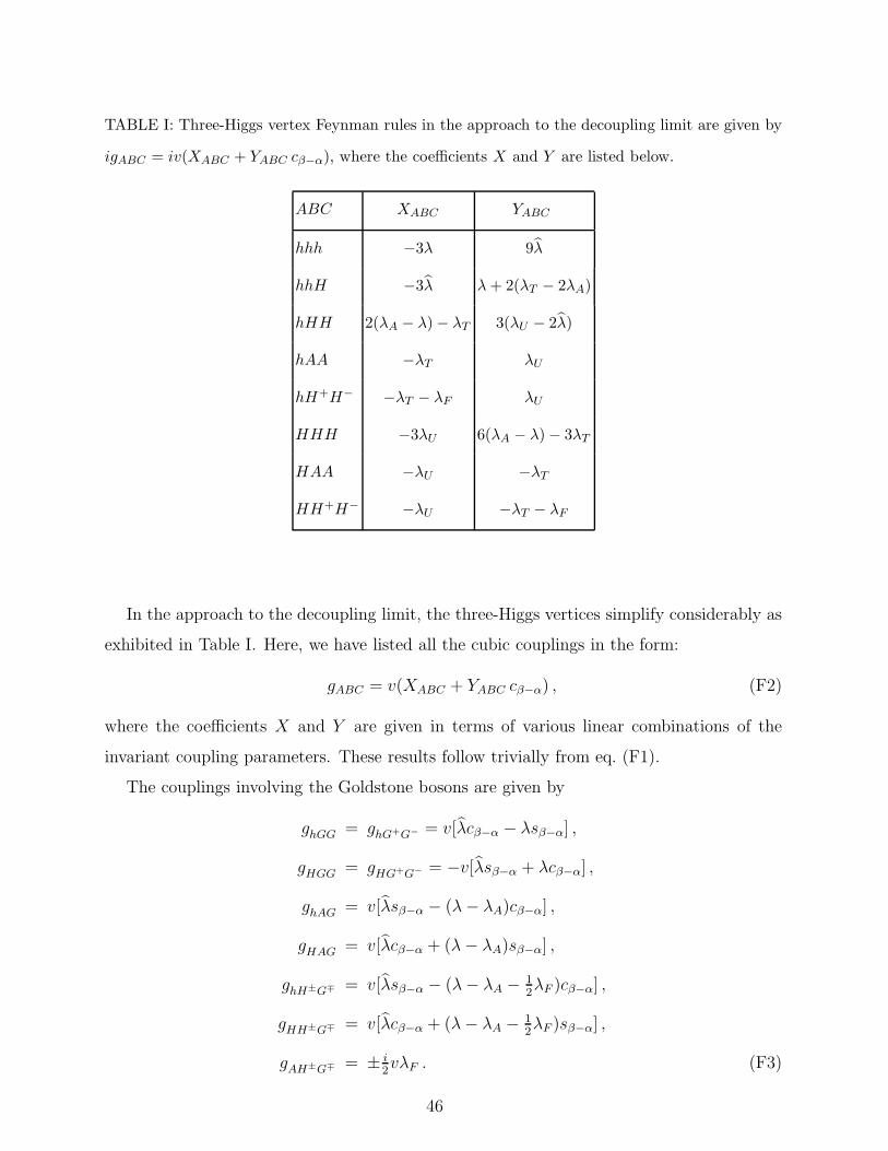
TABLE I: Three-Higgs vertex Feynman rules in the approach to the decoupling limit are given by

igABC = iv(XABC + YABC cβ−α), where the coefficients X and Y are listed below.

ABC XABC YABC

hhh −3λ 9λ

hhH −3λ λ + 2(λT − 2λA)

hHH 2(λA − λ) − λT 3(λU − 2λ)

hAA −λT λU

hH+H− −λT − λF λU

HHH −3λU 6(λA − λ) − 3λT

HAA −λU −λT

HH+H− −λU −λT − λF

In the approach to the decoupling limit, the three-Higgs vertices simplify considerably as

exhibited in Table I. Here, we have listed all the cubic couplings in the form:

gABC = v(XABC + YABC cβ−α) , (F2)

where the coefficients X and Y are given in terms of various linear combinations of the

invariant coupling parameters. These results follow trivially from eq. (F1).

The couplings involving the Goldstone bosons are given by

ghGG = ghG+G− = v[λcβ−α − λsβ−α] ,

gHGG = gHG+G− = −v[λsβ−α + λcβ−α] ,

ghAG = v[λsβ−α − (λ− λA)cβ−α] ,

gHAG = v[λcβ−α + (λ− λA)sβ−α] ,

ghH±G∓ = v[λsβ−α − (λ− λA − 12λF )cβ−α] ,

gHH±G∓ = v[λcβ−α + (λ− λA − 12λF )sβ−α] ,

gAH±G∓ = ± i2vλF . (F3)

46

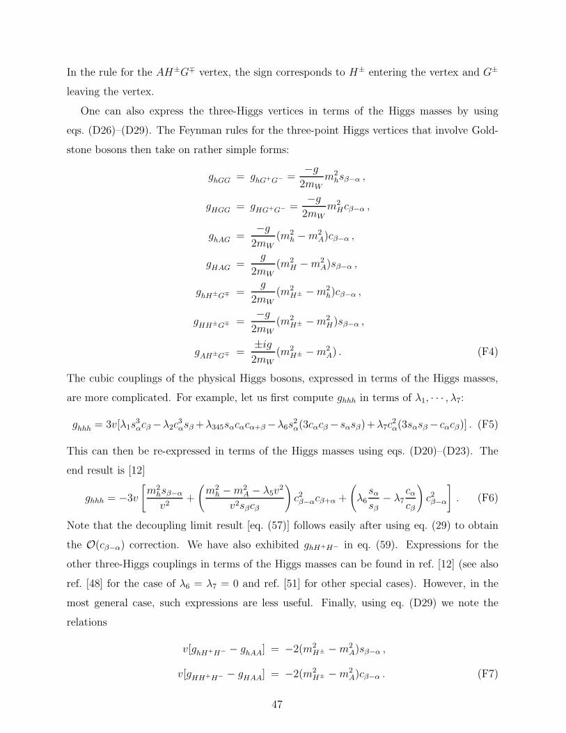
In the rule for the AH±G∓ vertex, the sign corresponds to H± entering the vertex and G±

leaving the vertex.

One can also express the three-Higgs vertices in terms of the Higgs masses by using

eqs. (D26)–(D29). The Feynman rules for the three-point Higgs vertices that involve Gold-

stone bosons then take on rather simple forms:

ghGG = ghG+G− =−g

2mWm2

hsβ−α ,

gHGG = gHG+G− =−g

2mWm2

Hcβ−α ,

ghAG =−g

2mW(m2

h −m2A)cβ−α ,

gHAG =g

2mW(m2

H −m2A)sβ−α ,

ghH±G∓ =g

2mW

(m2H± −m2

h)cβ−α ,

gHH±G∓ =−g

2mW(m2

H± −m2H)sβ−α ,

gAH±G∓ =±ig2mW

(m2H± −m2

A) . (F4)

The cubic couplings of the physical Higgs bosons, expressed in terms of the Higgs masses,

are more complicated. For example, let us first compute ghhh in terms of λ1, · · · , λ7:

ghhh = 3v[λ1s3αcβ −λ2c

3αsβ +λ345sαcαcα+β −λ6s

2α(3cαcβ −sαsβ)+λ7c

2α(3sαsβ − cαcβ)] . (F5)

This can then be re-expressed in terms of the Higgs masses using eqs. (D20)–(D23). The

end result is [12]

ghhh = −3v

[m2

hsβ−α

v2+

(m2

h −m2A − λ5v

2

v2sβcβ

)c2β−αcβ+α +

(λ6sα

sβ− λ7

cαcβ

)c2β−α

]. (F6)

Note that the decoupling limit result [eq. (57)] follows easily after using eq. (29) to obtain

the O(cβ−α) correction. We have also exhibited ghH+H− in eq. (59). Expressions for the

other three-Higgs couplings in terms of the Higgs masses can be found in ref. [12] (see also

ref. [48] for the case of λ6 = λ7 = 0 and ref. [51] for other special cases). However, in the

most general case, such expressions are less useful. Finally, using eq. (D29) we note the

relations

v[ghH+H− − ghAA] = −2(m2H± −m2

A)sβ−α ,

v[gHH+H− − gHAA] = −2(m2H± −m2

A)cβ−α . (F7)

47

APPENDIX G: FOUR-HIGGS VERTICES IN THE TWO-HIGGS DOUBLET

MODEL

In this Appendix, we list the Feynman rules for the four-point Higgs interaction in the

most general CP-conserving two-Higgs doublet extension of the Standard Model. Recalling

that Lint ∋ −V, the Feynman rules are obtained from the scalar potential33 by multiplying

the corresponding coefficients of V by −i times the appropriate symmetry factor. We find it

convenient to write the terms of the potential that are quartic in the Higgs fields as a sum

of two pieces: V ∋ VA + VB, where VA depends explicitly on β − α and VB is independent

of β − α. To obtain the four-Higgs couplings in terms of β − α and the invariant coupling

parameters, we insert eqs. (E3)–(E5) into eq. (E6), and identify the terms that are quartic

in the Higgs boson fields. For completeness, the quartic interaction terms involving the

Goldstone bosons (G± and G) are also listed. The end result is:

8VA =

h4[λs2

β−α(3c2β−α + 1) − 4λcβ−αs3β−α − 2(2λA − λT )c2β−αs

2β−α − 4λUc

3β−αsβ−α + λV c

4β−α

]

+4h3H[λsβ−αcβ−α(3c2β−α − 1) − λs2

β−α(4c2β−α − 1) − (2λA − λT )sβ−αcβ−α(c2β−α − s2β−α)

+λUc2β−α(4s2

β−α − 1) − λV sβ−αc3β−α

]

+2h2H2[λ(2 − 9s2

β−αc2β−α) − 6(λ− λU)sβ−αcβ−α(c2β−α − s2

β−α)

−(2λA − λT )(1 − 6s2β−αc

2β−α) + 3λV s

2β−αc

2β−α

]

+4hH3[λsβ−αcβ−α(3s2

β−α − 1) + λc2β−α(4s2β−α − 1) + (2λA − λT )sβ−αcβ−α(c2β−α − s2

β−α)

−λUs2β−α(4c2β−α − 1) − λV cβ−αs

3β−α

]

+H4[λc2β−α(3s2

β−α + 1) + 4λc3β−αsβ−α − 2(2λA − λT )c2β−αs2β−α + 4λUcβ−αs

3β−α + λV s

4β−α

]

+2h2A2[λT s

2β−α − 2λUsβ−αcβ−α + λV c

2β−α

]

+4h2AG[2(λ− λA)sβ−αcβ−α − λs2

β−α − λUc2β−α

]

+2h2G2[λs2

β−α − 2λsβ−αcβ−α + λT c2β−α

]

+4h2H+H−[(λT + λF )s2

β−α − 2λUsβ−αcβ−α + λV c2β−α

]

33 Note, e.g., that the term proportional to hAH+G− in V corresponds to H+ and G− directed into the

vertex, etc.

48

+4(h2H+G− + h2H−G+)[(2λ− 2λA − λF )sβ−αcβ−α − λs2

β−α − λUc2β−α

]

+4h2G+G−[λs2

β−α − 2λsβ−αcβ−α + (λT + λF )c2β−α

]

+4hHA2[(λT − λV )sβ−αcβ−α − λU(c2β−α − s2

β−α)]

+8hHAG[(λ− λA)(c2β−α − s2

β−α) − (λ− λU)sβ−αcβ−α)]

+4hHG2[(λ− λT )sβ−αcβ−α − λ(c2β−α − s2

β−α)]

+8hHH+H−[(λT − λV + λF )sβ−αcβ−α − λU(c2β−α − s2

β−α)]

+4(hHH+G− + hHH−G+)[(2λ− 2λA − λF )(c2β−α − s2

β−α) − 2(λ− λU)sβ−αcβ−α

]

+8hHG+G−[(λ− λT − λF )sβ−αcβ−α − λ(c2β−α − s2

β−α)]

+2H2A2[λT c

2β−α + 2λUsβ−αcβ−α + λV s

2β−α

]

+4H2AG[2(λA − λ)sβ−αcβ−α − λc2β−α − λUs

2β−α

]

+2H2G2[λc2β−α + 2λsβ−αcβ−α + λTs

2β−α

]

+4H2H+H−[(λT + λF )c2β−α + 2λUsβ−αcβ−α + λV s

2β−α

]

+4(H2H+G− +H2H−G+)[(2λA − 2λ+ λF )sβ−αcβ−α − λc2β−α − λUs

2β−α

]

+4H2G+G−[λc2β−α + 2λsβ−αcβ−α + (λT + λF )s2

β−α

]

+4i[hAH+G− − hAH−G+ +HGH+G− −HGH−G+

]λF sβ−α

−4i[hGH+G− − hGH−G+ −HAH+G− +HAH−G+

]λF cβ−α , (G1)

and

8VB = λV (A4 + 4A2H+H− + 4H+H−H+H−)

−4λU(A3G+ A2H+G− + A2H−G+ + 2AGH+H− + 2H+H−H+G− + 2H+H−H−G+)

+2 [2(λ− λA) + λT ]A2G2

+4(λT + λF )(A2G+G− +G2H+H−)

−4λ(AG3 + 2AGG+G− +G2H+G− +G2H−G+ + 2H+G+G−G− + 2H−G−G+G+)

+4 [2(λ− λA) − λF ] (AGH+G− + AGH−G+)

+λ(G4 + 4G2G+G− + 4G+G−G+G−)

+4(λ− λA)(H+H+G−G− +H−H−G+G+)

+8(λ− λA + λT )H+H−G+G− . (G2)

49

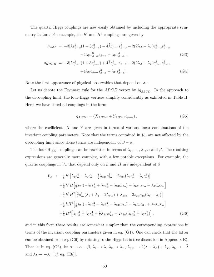
The quartic Higgs couplings are now easily obtained by including the appropriate sym-

metry factors. For example, the h4 and H4 couplings are given by

ghhhh = −3[λs2β−α(1 + 3c2β−α) − 4λcβ−αs

3β−α − 2(2λA − λT )c2β−αs

2β−α

−4λUc3β−αsβ−α + λV c

4β−α] , (G3)

gHHHH = −3[λc2β−α(1 + 3s2β−α) + 4λc3β−αsβ−α − 2(2λA − λT )c2β−αs

2β−α

+4λUcβ−αs3β−α + λV s

4β−α] . (G4)

Note the first appearance of physical observables that depend on λV .

Let us denote the Feynman rule for the ABCD vertex by igABCD. In the approach to

the decoupling limit, the four-Higgs vertices simplify considerably as exhibited in Table II.

Here, we have listed all couplings in the form:

gABCD = (XABCD + YABCD cβ−α) , (G5)

where the coefficients X and Y are given in terms of various linear combinations of the

invariant coupling parameters. Note that the terms contained in VB are not affected by the

decoupling limit since these terms are independent of β − α.

The four-Higgs couplings can be rewritten in terms of λ1, · · · , λ7, α and β. The resulting

expressions are generally more complex, with a few notable exceptions. For example, the

quartic couplings in VA that depend only on h and H are independent of β

VA ∋ 18h4[λ1s

4α + λ2c

4α + 1

2λ345s

22α − 2s2α(λ6s

2α + λ7c

2α)]

+12h3H

[12s2α(−λ1s

2α + λ2c

2α − λ345c2α) + λ6sαs3α + λ7cαc3α

]

+14h2H2

[34s22α(λ1 + λ2 − 2λ345) + λ345 − 3s2αc2α(λ6 − λ7)

]

+12hH3

[12s2α(−λ1c

2α + λ2s

2α + λ345c2α) + λ6cαc3α + λ7sαs3α

]

+18H4[λ1c

4α + λ2s

4α + 1

2λ345s

22α + 2s2α(λ6c

2α + λ7s

2α)], (G6)

and in this form these results are somewhat simpler than the corresponding expressions in

terms of the invariant coupling parameters given in eq. (G1). One can check that the latter

can be obtained from eq. (G6) by rotating to the Higgs basis (see discussion in Appendix E).

That is, in eq. (G6), let α → α − β, λ1 → λ, λ2 → λV , λ345 → 2(λ − λA) + λT , λ6 → −λand λ7 → −λU [cf. eq. (E6)].

50

TABLE II: Four-Higgs vertex Feynman rules in the approach to the decoupling limit are given by

igABCD = i(XABCD + YABCD cβ−α), where the coefficients X and Y are listed below. The rules

for AAAA, AAH+H−, and H+H−H+H− are exact (since they are independent of β − α).

ABCD XABCD YABCD

hhhh −3λ 12λ

hhhH −3λ 3(λ + λT − 2λA)

hhHH 2(λA − λ) − λT 6(λU − λ)

hhAA −λT 2λU

hhH+H− −λT − λF 2λU

hHHH −3λU 3(λV − λT ) + 6(λA − λ)

hHAA −λU −λT + λV

hHH+H− −λU λV − λT − λF

HHHH −3λV −12λU

HHAA −λV −2λU

HHH+H− −λV −2λU

AAAA −3λV 0

AAH+H− −λV 0

H+H−H+H− −2λV 0

One can also express the four-Higgs vertices in terms of the Higgs masses by using

eqs. (D20)–(D23). For example [12],

ghhhh = −3

m

2h

v2

(sβ−α − cβ+αc

2β−α

sβcβ

)2

+m2

H

v2

(sαcαcβ−α

sβcβ

)2

−m2A + λ5v

2

v2

(cβ+αcβ−α

sβcβ

)2

− 2(λ6s2α + λ7c

2α)c2β−α

sβcβ

. (G7)

Note that the decoupling limit result [eq. (58)] follows trivially, after using eqs. (29) and

(31) to obtain the O(cβ−α) correction. Expressions for other four-Higgs couplings in terms

51

of the Higgs masses can be found in ref. [12] (see also ref. [48] for the case of λ6 = λ7 = 0

and ref. [51] for other special cases). However, in the most general case, such expressions

are less useful.

[1] See, e.g., L. Susskind, Phys. Rept. 104 (1984) 181.

[2] E. Witten, Nucl. Phys. B188, 513 (1981); R.K. Kaul, Phys. Lett. 109B, 19 (1982); Pramana

19, 183 (1982).

[3] H.P. Nilles, Phys. Rept. 110, 1 (1984). H.E. Haber and G.L. Kane, Phys. Rept. 117, 75

(1985); S.P. Martin, hep-ph/9709356.

[4] S. Dimopoulos and H. Georgi, Nucl. Phys. B193, 150 (1981); K. Harada and N. Sakai, Prog.

Theor. Phys. 67, 1877 (1982); K. Inoue, A. Kakuto, H. Komatsu and S. Takeshita, Prog.

Theor. Phys. 67, 1889 (1982); L. Girardello and M.T. Grisaru, Nucl. Phys. B194, 65 (1982).

[5] E. Farhi and L. Susskind, Phys. Rept. 74, 277 (1981); R.K. Kaul, Rev. Mod. Phys. 55, 449

(1983); C.T. Hill and E.H. Simmons, FERMI-PUB-02/045-T [hep-ph/0203079].

[6] I. Antoniadis, Phys. Lett. B246, 377 (1990); N. Arkani-Hamed, S. Dimopoulos and G.R. Dvali,

Phys. Lett. B429, 263 (1998); L. Randall and R. Sundrum, Phys. Rev. Lett. 83, 3370 (1999).

For a review, see V.A. Rubakov, Phys. Usp. 44, 871 (2001) [Usp. Fiz. Nauk 171, 913 (2001)].

[7] J.F. Gunion, H.E. Haber, G. Kane and S. Dawson, The Higgs Hunter’s Guide (Perseus Pub-

lishing, Cambridge, MA, 1990).

[8] K. Inoue, A. Kakuto, H. Komatsu, and S. Takeshita, Prog. Theor. Phys. 68, 927 (1982) [E:

70, 330 (1983)]; R. Flores and M. Sher, Annals Phys. 148, 95 (1983).

[9] J.F. Gunion and H.E. Haber, Nucl. Phys. B 272, 1 (1986) [E: B402, 567 (1993)]; B278, 449

(1986).

[10] H.E. Haber and Y. Nir, Nucl. Phys. B335, 363 (1990).

[11] H.E. Haber, in Physics From the Planck Scale to the Electroweak Scale, Proceedings of the

US–Polish Workshop, Warsaw, Poland, September 21–24, 1994, edited by P. Nath, T. Taylor,

and S. Pokorski (World Scientific, Singapore, 1995) pp. 49–63.

[12] F. Boudjema and A. Semenov, Phys. Rev. D66, 095007 (2002).

[13] M.N. Dubinin and A.V. Semenov, hep-ph/0206205, Eur. J. Phys. C in press.

[14] J.F. Gunion, H.E. Haber and J. Kalinowski, in preparation.

52

[15] L.J. Hall and M.B. Wise, Nucl. Phys. B187, 397 (1981).

[16] S.L. Glashow and S. Weinberg, Phys. Rev. D15, 1958 (1977); E.A. Paschos, Phys. Rev. D15,

1966 (1977).

[17] W.S. Hou, Phys. Lett. B296, 179 (1992); D. Chang, W.S. Hou and W.Y. Keung, Phys. Rev.

D48, 217 (1993); D. Atwood, L. Reina and A. Soni, Phys. Rev. D55, 3156 (1997).

[18] N.G. Deshpande and E. Ma, Phys. Rev. D18, 2574 (1978); K.S. Babu and E. Ma, Phys. Rev.

D31, 2861 (1985) [E: D33, 3471 (1986)].

[19] J.M. Cornwall, D.N. Levin and G. Tiktopoulos, Phys. Rev. Lett. 30 (1973) 1268 [E: 31 (1973)

572]; Phys. Rev. D10, 1145 (1974) [E: D11, 972 (1975)]; C.H. Llewellyn Smith, Phys. Lett.

46B (1973) 233.

[20] B.W. Lee, C. Quigg and H.B. Thacker, Phys. Rev. D16, 1519 (1977).

[21] H.A. Weldon, Phys. Rev. D30, 1547 (1984).

[22] A.G. Akeroyd, A. Arhrib and E.M. Naimi, Phys. Lett. B490 (2000) 119; A. Arhrib,

hep-ph/0012353.

[23] S. Kanemura, T. Kubota and E. Takasugi, Phys. Lett. B313, 155 (1993).

[24] P. Ciafaloni and D. Espriu, Phys. Rev. D56, 1752 (1997)

[25] R.A. Diaz, R. Martinez and J.-Alexis Rodriguez, Phys. Rev. D63, 095007 (2001).

[26] A. Sirlin and R. Zucchini, Nucl. Phys. B266, 389 (1986).

[27] M. Luscher and P. Weisz, Phys. Lett. B212, 472 (1988).

[28] T. Appelquist and J. Carazzone, Phys. Rev. D11 (1975) 2856.

[29] I.F. Ginzburg, M. Krawczyk and P. Osland, Nucl. Instrum. Meth. A472, 149 (2001); and in

Physics and experiments with future linear e+e− colliders, Proceedings of the 5th International

Linear Collider Workshop, Batavia, IL, USA, 2000, edited by A. Para and H.E. Fisk (American

Institute of Physics, New York, 2001), pp. 304–311 [hep-ph/0101331]; contribution to the 2nd

ECFA/DESY Study, hep-ph/0101208.

[30] S. Kanemura, S. Kiyoura, Y. Okada, E. Senaha and C.P. Yuan, KEK-TH-856 and MSUHEP-

21119 [hep-ph/0211308].

[31] P. Chankowski, T. Farris, B. Grzadkowski, J.F. Gunion, J. Kalinowski and M. Krawczyk,

Phys. Lett. B496, 195 (2000).

[32] A. Djouadi, V. Driesen, W. Hollik and J.I. Illana, Eur. Phys. J. C1, 149 (1998); A. Djouadi,

Phys. Lett. B435, 101 (1998); C. S. Huang and X.H. Wu, Phys. Rev. D66, 075002 (2002).

53

[33] A. Dobado, M.J. Herrero and S. Penaranda, Eur. Phys. J. C7, 313 (1999).

[34] S. Heinemeyer, W. Hollik and G. Weiglein, Eur. Phys. J. C16, 139 (2000).

[35] L.J. Hall, R. Rattazzi and U. Sarid, Phys. Rev. D50, 7048 (1994); R. Hempfling, Phys. Rev.

D49, 6168 (1994).

[36] M. Carena, M. Olechowski, S. Pokorski and C.E.M. Wagner, Nucl. Phys. B426, 269 (1994).

[37] A. Bartl, H. Eberl, K. Hikasa, T. Kon, W. Majerotto and Y. Yamada, Phys. Lett. B378, 167

(1996); R.A. Jimenez and J. Sola, Phys. Lett. B389, 53 (1996); J.A. Coarasa, R.A. Jimenez

and J. Sola, Phys. Lett. B389, 312 (1996).

[38] D.M. Pierce, J.A. Bagger, K. Matchev, and R. Zhang, Nucl. Phys. B491, 3 (1997).

[39] M. Carena, H.E. Haber, H.E. Logan and S. Mrenna, Phys. Rev. D65, 055005 (2002) [E: D65,

099902 (2002)].

[40] M. Carena and H.E. Haber, FERMILAB-Pub-02/114-T and SCIPP 02/07 [hep-ph/0208209],

Prog. Part. Nucl. Phys., in press.

[41] H.E. Haber, M.J. Herrero, H.E. Logan, S. Penaranda, S. Rigolin and D. Temes, Phys. Rev.

D63, 055004 (2001).

[42] C.P. Burgess, J. Matias and M. Pospelov, Int. J. Mod. Phys. A17, 1841 (2002).

[43] L. Lavoura and J.P. Silva, Phys. Rev. D50, 4619 (1994); F.J. Botella and J.P. Silva, Phys.

Rev. D51, 3870 (1995).

[44] G.C. Branco, L. Lavoura and J.P. Silva, CP Violation (Oxford University Press, Oxford,

England, 1999), chapters 22 and 23.

[45] T.D. Lee, Phys. Rev. D8, 1226 (1973).

[46] J. Velhinho, R. Santos and A. Barroso, Phys. Lett. B322 (1994) 213.

[47] C. Lin, C. Lee and Y.-W. Yang, Phys. Rev. D50, 558 (1994).

[48] M.N. Dubinin and A.V. Semenov, hep-ph/9812246. This paper contains a number of sign

errors. For example, in the hhhh coupling, the relative sign between two terms in the coefficient

multiplying m2h is incorrect. The correct factor is c3

αcβ − s3αsβ = sβcβsβ−α + cβ+αc2

β−α. In

deriving this last result, one makes use of the remarkable identity: sβcβ − sαcα = cβ+αsβ−α.

[49] R. Santos, S.M. Oliveira and A. Barroso, hep-ph/0112202.

[50] J.F. Gunion and H.E. Haber, in preparation.

[51] R. Santos and A. Barroso, Phys. Rev. D56, 5366 (1997); L. Brucher and R. Santos, Eur.

Phys. J. C12, 87 (2000).

54