university of california, los angeles department of statistics introduction to...
TRANSCRIPT

University of California, Los AngelesDepartment of Statistics
Introduction to GRASS/R spatial data analysis
• What is Geographic Information Systems (GIS)?
- “A geographic information system (GIS) integrates hardware, software, and data for capturing,managing, analyzing, and displaying all forms of geographically referenced information.” (ESRI,http://www.gis.com).
- “GIS are tools that allow for the processing of spatial data into information and used to makedecisions about some portion of the earth.” (Fundamentals of Geographic Information Systems,DeMers. M., Third Edition, 2005)
- “GIS is often described as integration of data, hardware, and software designed for management,processing, analysis, and visualization of georeferenced data.” (OPEN SOURCE GIS, A GRASSGIS APPROACH, Neteler, M., Mitasova, H., Third Edition (2008).
• Why GIS?Needed for map analysis operations in areas such as
- Forestry
- Fire Departments
- Police Departments
- EMS
- Traffic
- Water resources
- Real estate
- Military
- Business
- Mining, geology
- Hydrology
- Wildlife management
- Epidemiology
- Agriculture
- Election results
- Etc.
Useful tool for statisticians that work with spatial data.
• Geographical Data: Four main components.
- Input
- Administration
- Analysis
- Presentation
1

• With GIS we can study
- Land
- Elevation
- Forests
- Population densities
- Energy consumption
- Mineral resources, etc.
• A GIS map has layers. Each layer represents geographic objects that are similar. For example, citiescan be one layer, rivers another one, roads, lakes, etc. With a click of a button, we can include allthese layers on our GIS map, or simply have as many layers as we want.
• GIS can help us understood our geographic data easily.
• 3D visualization and animation (see snapshot below from GRASS):
2
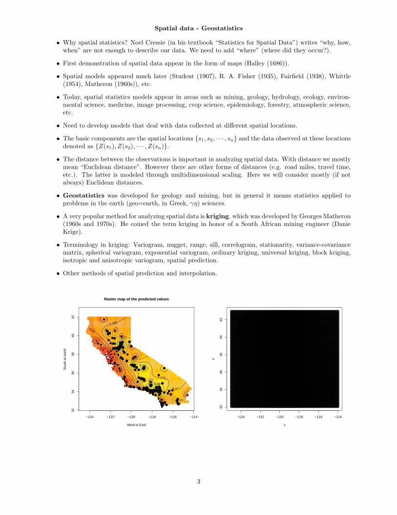
Spatial data - Geostatistics
• Why spatial statistics? Noel Cressie (in his textbook “Statistics for Spatial Data”) writes “why, how,when” are not enough to describe our data. We need to add “where” (where did they occur?).
• First demonstration of spatial data appear in the form of maps (Halley (1686)).
• Spatial models appeared much later (Student (1907), R. A. Fisher (1935), Fairfield (1938), Whittle(1954), Matheron (1960s)), etc.
• Today, spatial statistics models appear in areas such as mining, geology, hydrology, ecology, environ-mental science, medicine, image processing, crop science, epidemiology, forestry, atmospheric science,etc.
• Need to develop models that deal with data collected at different spatial locations.
• The basic components are the spatial locations {s1, s2, · · · , sn} and the data observed at these locationsdenoted as {Z(s1), Z(s2), · · · , Z(sn)}.
• The distance between the observations is important in analyzing spatial data. With distance we mostlymean “Euclidean distance”. However there are other forms of distances (e.g. road miles, travel time,etc.). The latter is modeled through multidimensional scaling. Here we will consider mostly (if notalways) Euclidean distances.
• Geostatistics was developed for geology and mining, but in general it means statistics applied toproblems in the earth (geo=earth, in Greek, γη) sciences.
• A very popular method for analyzing spatial data is kriging, which was developed by Georges Matheron(1960s and 1970s). He coined the term kriging in honor of a South African mining engineer (DanieKrige).
• Terminology in kriging: Variogram, nugget, range, sill, correlogram, stationarity, variance-covariancematrix, spherical variogram, exponential variogram, ordinary kriging, universal kriging, block kriging,isotropic and anisotropic variogram, spatial prediction.
• Other methods of spatial prediction and interpolation.
−124 −122 −120 −118 −116 −114
3234
3638
4042
Raster map of the predicted values
West to East
Sou
th to
Nor
th
0.05
0.05
0.055
0.06
0.06
0.065
0.07
0.07
0.07
0.07
0.075
0.08
0.08 0.08
●
●●
●
●
●●
●●
●
●
●
●
●
●
●●
●
●
●
●
●
●
●
●
●
●
●
●
●
●
●
●
●●
●
● ●●●●
●
●
●
●
●
●
●
●
●
●
●
●
●
●
●
●
●
●
●
●
●
●
●
●
●●
●
●
●
●●
●
●●
●
●
●
●
●
●
●
●
●
●
●
●
●
●
●
●
●
●
●
●
●
●
●
●
●
●
●
●
●●
●
●
●
●
●
●
●
●
●
●
●
●
●
●
●
●
●
●
●
●
●
●
●●
●
●
●
●
●
●
●
●
●●
●
●●
●
●
●
●
●
●
●●
●
●
●
●
●
●
●
●
●
●
●●●
●
●
●
●
●
●
●●
●
●
●
●
●●●●●●●●●●●●●●●●●●●●●●●●●●●●●●●●●●●●●●●●●●●●●●●●●●●●●●●●●●●●●●●●●●●●●●●●●●●●●●●●●●●●●●●●●●●●●●●●●●●●●●●●●●●●●●●●●●●●●●●●●●●●●●●●●●●●●●●●●●●●●●●●●●●●●●●●●●●●●●●●●●●●●●●●●●●●●●●●●●●●●●●●●●●●●●●●●●●●●●●●●●●●●●●●●●●●●●●●●●●●●●●●●●●●●●●●●●●●●●●●●●●●●●●●●●●●●●●●●●●●●●●●●●●●●●●●●●●●●●●●●●●●●●●●●●●●●●●●●●●●●●●●●●●●●●●●●●●●●●●●●●●●●●●●●●●●●●●●●●●●●●●●●●●●●●●●●●●●●●●●●●●●●●●●●●●●●●●●●●●●●●●●●●●●●●●●●●●●●●●●●●●●●●●●●●●●●●●●●●●●●●●●●●●●●●●●●●●●●●●●●●●●●●●●●●●●●●●●●●●●●●●●●●●●●●●●●●●●●●●●●●●●●●●●●●●●●●●●●●●●●●●●●●●●●●●●●●●●●●●●●●●●●●●●●●●●●●●●●●●●●●●●●●●●●●●●●●●●●●●●●●●●●●●●●●●●●●●●●●●●●●●●●●●●●●●●●●●●●●●●●●●●●●●●●●●●●●●●●●●●●●●●●●●●●●●●●●●●●●●●●●●●●●●●●●●●●●●●●●●●●●●●●●●●●●●●●●●●●●●●●●●●●●●●●●●●●●●●●●●●●●●●●●●●●●●●●●●●●●●●●●●●●●●●●●●●●●●●●●●●●●●●●●●●●●●●●●●●●●●●●●●●●●●●●●●●●●●●●●●●●●●●●●●●●●●●●●●●●●●●●●●●●●●●●●●●●●●●●●●●●●●●●●●●●●●●●●●●●●●●●●●●●●●●●●●●●●●●●●●●●●●●●●●●●●●●●●●●●●●●●●●●●●●●●●●●●●●●●●●●●●●●●●●●●●●●●●●●●●●●●●●●●●●●●●●●●●●●●●●●●●●●●●●●●●●●●●●●●●●●●●●●●●●●●●●●●●●●●●●●●●●●●●●●●●●●●●●●●●●●●●●●●●●●●●●●●●●●●●●●●●●●●●●●●●●●●●●●●●●●●●●●●●●●●●●●●●●●●●●●●●●●●●●●●●●●●●●●●●●●●●●●●●●●●●●●●●●●●●●●●●●●●●●●●●●●●●●●●●●●●●●●●●●●●●●●●●●●●●●●●●●●●●●●●●●●●●●●●●●●●●●●●●●●●●●●●●●●●●●●●●●●●●●●●●●●●●●●●●●●●●●●●●●●●●●●●●●●●●●●●●●●●●●●●●●●●●●●●●●●●●●●●●●●●●●●●●●●●●●●●●●●●●●●●●●●●●●●●●●●●●●●●●●●●●●●●●●●●●●●●●●●●●●●●●●●●●●●●●●●●●●●●●●●●●●●●●●●●●●●●●●●●●●●●●●●●●●●●●●●●●●●●●●●●●●●●●●●●●●●●●●●●●●●●●●●●●●●●●●●●●●●●●●●●●●●●●●●●●●●●●●●●●●●●●●●●●●●●●●●●●●●●●●●●●●●●●●●●●●●●●●●●●●●●●●●●●●●●●●●●●●●●●●●●●●●●●●●●●●●●●●●●●●●●●●●●●●●●●●●●●●●●●●●●●●●●●●●●●●●●●●●●●●●●●●●●●●●●●●●●●●●●●●●●●●●●●●●●●●●●●●●●●●●●●●●●●●●●●●●●●●●●●●●●●●●●●●●●●●●●●●●●●●●●●●●●●●●●●●●●●●●●●●●●●●●●●●●●●●●●●●●●●●●●●●●●●●●●●●●●●●●●●●●●●●●●●●●●●●●●●●●●●●●●●●●●●●●●●●●●●●●●●●●●●●●●●●●●●●●●●●●●●●●●●●●●●●●●●●●●●●●●●●●●●●●●●●●●●●●●●●●●●●●●●●●●●●●●●●●●●●●●●●●●●●●●●●●●●●●●●●●●●●●●●●●●●●●●●●●●●●●●●●●●●●●●●●●●●●●●●●●●●●●●●●●●●●●●●●●●●●●●●●●●●●●●●●●●●●●●●●●●●●●●●●●●●●●●●●●●●●●●●●●●●●●●●●●●●●●●●●●●●●●●●●●●●●●●●●●●●●●●●●●●●●●●●●●●●●●●●●●●●●●●●●●●●●●●●●●●●●●●●●●●●●●●●●●●●●●●●●●●●●●●●●●●●●●●●●●●●●●●●●●●●●●●●●●●●●●●●●●●●●●●●●●●●●●●●●●●●●●●●●●●●●●●●●●●●●●●●●●●●●●●●●●●●●●●●●●●●●●●●●●●●●●●●●●●●●●●●●●●●●●●●●●●●●●●●●●●●●●●●●●●●●●●●●●●●●●●●●●●●●●●●●●●●●●●●●●●●●●●●●●●●●●●●●●●●●●●●●●●●●●●●●●●●●●●●●●●●●●●●●●●●●●●●●●●●●●●●●●●●●●●●●●●●●●●●●●●●●●●●●●●●●●●●●●●●●●●●●●●●●●●●●●●●●●●●●●●●●●●●●●●●●●●●●●●●●●●●●●●●●●●●●●●●●●●●●●●●●●●●●●●●●●●●●●●●●●●●●●●●●●●●●●●●●●●●●●●●●●●●●●●●●●●●●●●●●●●●●●●●●●●●●●●●●●●●●●●●●●●●●●●●●●●●●●●●●●●●●●●●●●●●●●●●●●●●●●●●●●●●●●●●●●●●●●●●●●●●●●●●●●●●●●●●●●●●●●●●●●●●●●●●●●●●●●●●●●●●●●●●●●●●●●●●●●●●●●●●●●●●●●●●●●●●●●●●●●●●●●●●●●●●●●●●●●●●●●●●●●●●●●●●●●●●●●●●●●●●●●●●●●●●●●●●●●●●●●●●●●●●●●●●●●●●●●●●●●●●●●●●●●●●●●●●●●●●●●●●●●●●●●●●●●●●●●●●●●●●●●●●●●●●●●●●●●●●●●●●●●●●●●●●●●●●●●●●●●●●●●●●●●●●●●●●●●●●●●●●●●●●●●●●●●●●●●●●●●●●●●●●●●●●●●●●●●●●●●●●●●●●●●●●●●●●●●●●●●●●●●●●●●●●●●●●●●●●●●●●●●●●●●●●●●●●●●●●●●●●●●●●●●●●●●●●●●●●●●●●●●●●●●●●●●●●●●●●●●●●●●●●●●●●●●●●●●●●●●●●●●●●●●●●●●●●●●●●●●●●●●●●●●●●●●●●●●●●●●●●●●●●●●●●●●●●●●●●●●●●●●●●●●●●●●●●●●●●●●●●●●●●●●●●●●●●●●●●●●●●●●●●●●●●●●●●●●●●●●●●●●●●●●●●●●●●●●●●●●●●●●●●●●●●●●●●●●●●●●●●●●●●●●●●●●●●●●●●●●●●●●●●●●●●●●●●●●●●●●●●●●●●●●●●●●●●●●●●●●●●●●●●●●●●●●●●●●●●●●●●●●●●●●●●●●●●●●●●●●●●●●●●●●●●●●●●●●●●●●●●●●●●●●●●●●●●●●●●●●●●●●●●●●●●●●●●●●●●●●●●●●●●●●●●●●●●●●●●●●●●●●●●●●●●●●●●●●●●●●●●●●●●●●●●●●●●●●●●●●●●●●●●●●●●●●●●●●●●●●●●●●●●●●●●●●●●●●●●●●●●●●●●●●●●●●●●●●●●●●●●●●●●●●●●●●●●●●●●●●●●●●●●●●●●●●●●●●●●●●●●●●●●●●●●●●●●●●●●●●●●●●●●●●●●●●●●●●●●●●●●●●●●●●●●●●●●●●●●●●●●●●●●●●●●●●●●●●●●●●●●●●●●●●●●●●●●●●●●●●●●●●●●●●●●●●●●●●●●●●●●●●●●●●●●●●●●●●●●●●●●●●●●●●●●●●●●●●●●●●●●●●●●●●●●●●●●●●●●●●●●●●●●●●●●●●●●●●●●●●●●●●●●●●●●●●●●●●●●●●●●●●●●●●●●●●●●●●●●●●●●●●●●●●●●●●●●●●●●●●●●●●●●●●●●●●●●●●●●●●●●●●●●●●●●●●●●●●●●●●●●●●●●●●●●●●●●●●●●●●●●●●●●●●●●●●●●●●●●●●●●●●●●●●●●●●●●●●●●●●●●●●●●●●●●●●●●●●●●●●●●●●●●●●●●●●●●●●●●●●●●●●●●●●●●●●●●●●●●●●●●●●●●●●●●●●●●●●●●●●●●●●●●●●●●●●●●●●●●●●●●●●●●●●●●●●●●●●●●●●●●●●●●●●●●●●●●●●●●●●●●●●●●●●●●●●●●●●●●●●●●●●●●●●●●●●●●●●●●●●●●●●●●●●●●●●●●●●●●●●●●●●●●●●●●●●●●●●●●●●●●●●●●●●●●●●●●●●●●●●●●●●●●●●●●●●●●●●●●●●●●●●●●●●●●●●●●●●●●●●●●●●●●●●●●●●●●●●●●●●●●●●●●●●●●●●●●●●●●●●●●●●●●●●●●●●●●●●●●●●●●●●●●●●●●●●●●●●●●●●●●●●●●●●●●●●●●●●●●●●●●●●●●●●●●●●●●●●●●●●●●●●●●●●●●●●●●●●●●●●●●●●●●●●●●●●●●●●●●●●●●●●●●●●●●●●●●●●●●●●●●●●●●●●●●●●●●●●●●●●●●●●●●●●●●●●●●●●●●●●●●●●●●●●●●●●●●●●●●●●●●●●●●●●●●●●●●●●●●●●●●●●●●●●●●●●●●●●●●●●●●●●●●●●●●●●●●●●●●●●●●●●●●●●●●●●●●●●●●●●●●●●●●●●●●●●●●●●●●●●●●●●●●●●●●●●●●●●●●●●●●●●●●●●●●●●●●●●●●●●●●●●●●●●●●●●●●●●●●●●●●●●●●●●●●●●●●●●●●●●●●●●●●●●●●●●●●●●●●●●●●●●●●●●●●●●●●●●●●●●●●●●●●●●●●●●●●●●●●●●●●●●●●●●●●●●●●●●●●●●●●●●●●●●●●●●●●●●●●●●●●●●●●●●●●●●●●●●●●●●●●●●●●●●●●●●●●●●●●●●●●●●●●●●●●●●●●●●●●●●●●●●●●●●●●●●●●●●●●●●●●●●●●●●●●●●●●●●●●●●●●●●●●●●●●●●●●●●●●●●●●●●●●●●●●●●●●●●●●●●●●●●●●●●●●●●●●●●●●●●●●●●●●●●●●●●●●●●●●●●●●●●●●●●●●●●●●●●●●●●●●●●●●●●●●●●●●●●●●●●●●●●●●●●●●●●●●●●●●●●●●●●●●●●●●●●●●●●●●●●●●●●●●●●●●●●●●●●●●●●●●●●●●●●●●●●●●●●●●●●●●●●●●●●●●●●●●●●●●●●●●●●●●●●●●●●●●●●●●●●●●●●●●●●●●●●●●●●●●●●●●●●●●●●●●●●●●●●●●●●●●●●●●●●●●●●●●●●●●●●●●●●●●●●●●●●●●●●●●●●●●●●●●●●●●●●●●●●●●●●●●●●●●●●●●●●●●●●●●●●●●●●●●●●●●●●●●●●●●●●●●●●●●●●●●●●●●●●●●●●●●●●●●●●●●●●●●●●●●●●●●●●●●●●●●●●●●●●●●●●●●●●●●●●●●●●●●●●●●●●●●●●●●●●●●●●●●●●●●●●●●●●●●●●●●●●●●●●●●●●●●●●●●●●●●●●●●●●●●●●●●●●●●●●●●●●●●●●●●●●●●●●●●●●●●●●●●●●●●●●●●●●●●●●●●●●●●●●●●●●●●●●●●●●●●●●●●●●●●●●●●●●●●●●●●●●●●●●●●●●●●●●●●●●●●●●●●●●●●●●●●●●●●●●●●●●●●●●●●●●●●●●●●●●●●●●●●●●●●●●●●●●●●●●●●●●●●●●●●●●●●●●●●●●●●●●●●●●●●●●●●●●●●●●●●●●●●●●●●●●●●●●●●●●●●●●●●●●●●●●●●●●●●●●●●●●●●●●●●●●●●●●●●●●●●●●●●●●●●●●●●●●●●●●●●●●●●●●●●●●●●●●●●●●●●●●●●●●●●●●●●●●●●●●●●●●●●●●●●●●●●●●●●●●●●●●●●●●●●●●●●●●●●●●●●●●●●●●●●●●●●●●●●●●●●●●●●●●●●●●●●●●●●●●●●●●●●●●●●●●●●●●●●●●●●●●●●●●●●●●●●●●●●●●●●●●●●●●●●●●●●●●●●●●●●●●●●●●●●●●●●●●●●●●●●●●●●●●●●●●●●●●●●●●●●●●●●●●●●●●●●●●●●●●●●●●●●●●●●●●●●●●●●●●●●●●●●●●●●●●●●●●●●●●●●●●●●●●●●●●●●●●●●●●●●●●●●●●●●●●●●●●●●●●●●●●●●●●●●●●●●●●●●●●●●●●●●●●●●●●●●●●●●●●●●●●●●●●●●●●●●●●●●●●●●●●●●●●●●●●●●●●●●●●●●●●●●●●●●●●●●●●●●●●●●●●●●●●●●●●●●●●●●●●●●●●●●●●●●●●●●●●●●●●●●●●●●●●●●●●●●●●●●●●●●●●●●●●●●●●●●●●●●●●●●●●●●●●●●●●●●●●●●●●●●●●●●●●●●●●●●●●●●●●●●●●●●●●●●●●●●●●●●●●●●●●●●●●●●●●●●●●●●●●●●●●●●●●●●●●●●●●●●●●●●●●●●●●●●●●●●●●●●●●●●●●●●●●●●●●●●●●●●●●●●●●●●●●●●●●●●●●●●●●●●●●●●●●●●●●●●●●●●●●●●●●●●●●●●●●●●●●●●●●●●●●●●●●●●●●●●●●●●●●●●●●●●●●●●●●●●●●●●●●●●●●●●●●●●●●●●●●●●●●●●●●●●●●●●●●●●●●●●●●●●●●●●●●●●●●●●●●●●●●●●●●●●●●●●●●●●●●●●●●●●●●●●●●●●●●●●●●●●●●●●●●●●●●●●●●●●●●●●●●●●●●●●●●●●●●●●●●●●●●●●●●●●●●●●●●●●●●●●●●●●●●●●●●●●●●●●●●●●●●●●●●●●●●●●●●●●●●●●●●●●●●●●●●●●●●●●●●●●●●●●●●●●●●●●●●●●●●●●●●●●●●●●●●●●●●●●●●●●●●●●●●●●●●●●●●●●●●●●●●●●●●●●●●●●●●●●●●●●●●●●●●●●●●●●●●●●●●●●●●●●●●●●●●●●●●●●●●●●●●●●●●●●●●●●●●●●●●●●●●●●●●●●●●●●●●●●●●●●●●●●●●●●●●●●●●●●●●●●●●●●●●●●●●●●●●●●●●●●●●●●●●●●●●●●●●●●●●●●●●●●●●●●●●●●●●●●●●●●●●●●●●●●●●●●●●●●●●●●●●●●●●●●●●●●●●●●●●●●●●●●●●●●●●●●●●●●●●●●●●●●●●●●●●●●●●●●●●●●●●●●●●●●●●●●●●●●●●●●●●●●●●●●●●●●●●●●●●●●●●●●●●●●●●●●●●●●●●●●●●●●●●●●●●●●●●●●●●●●●●●●●●●●●●●●●●●●●●●●●●●●●●●●●●●●●●●●●●●●●●●●●●●●●●●●●●●●●●●●●●●●●●●●●●●●●●●●●●●●●●●●●●●●●●●●●●●●●●●●●●●●●●●●●●●●●●●●●●●●●●●●●●●●●●●●●●●●●●●●●●●●●●●●●●●●●●●●●●●●●●●●●●●●●●●●●●●●●●●●●●●●●●●●●●●●●●●●●●●●●●●●●●●●●●●●●●●●●●●●●●●●●●●●●●●●●●●●●●●●●●●●●●●●●●●●●●●●●●●●●●●●●●●●●●●●●●●●●●●●●●●●●●●●●●●●●●●●●●●●●●●●●●●●●●●●●●●●●●●●●●●●●●●●●●●●●●●●●●●●●●●●●●●●●●●●●●●●●●●●●●●●●●●●●●●●●●●●●●●●●●●●●●●●●●●●●●●●●●●●●●●●●●●●●●●●●●●●●●●●●●●●●●●●●●●●●●●●●●●●●●●●●●●●●●●●●●●●●●●●●●●●●●●●●●●●●●●●●●●●●●●●●●●●●●●●●●●●●●●●●●●●●●●●●●●●●●●●●●●●●●●●●●●●●●●●●●●●●●●●●●●●●●●●●●●●●●●●●●●●●●●●●●●●●●●●●●●●●●●●●●●●●●●●●●●●●●●●●●●●●●●●●●●●●●●●●●●●●●●●●●●●●●●●●●●●●●●●●●●●●●●●●●●●●●●●●●●●●●●●●●●●●●●●●●●●●●●●●●●●●●●●●●●●●●●●●●●●●●●●●●●●●●●●●●●●●●●●●●●●●●●●●●●●●●●●●●●●●●●●●●●●●●●●●●●●●●●●●●●●●●●●●●●●●●●●●●●●●●●●●●●●●●●●●●●●●●●●●●●●●●●●●●●●●●●●●●●●●●●●●●●●●●●●●●●●●●●●●●●●●●●●●●●●●●●●●●●●●●●●●●●●●●●●●●●●●●●●●●●●●●●●●●●●●●●●●●●●●●●●●●●●●●●●●●●●●●●●●●●●●●●●●●●●●●●●●●●●●●●●●●●●●●●●●●●●●●●●●●●●●●●●●●●●●●●●●●●●●●●●●●●●●●●●●●●●●●●●●●●●●●●●●●●●●●●●●●●●●●●●●●●●●●●●●●●●●●●●●●●●●●●●●●●●●●●●●●●●●●●●●●●●●●●●●●●●●●●●●●●●●●●●●●●●●●●●●●●●●●●●●●●●●●●●●●●●●●●●●●●●●●●●●●●●●●●●●●●●●●●●●●●●●●●●●●●●●●●●●●●●●●●●●●●●●●●●●●●●●●●●●●●●●●●●●●●●●●●●●●●●●●●●●●●●●●●●●●●●●●●●●●●●●●●●●●●●●●●●●●●●●●●●●●●●●●●●●●●●●●●●●●●●●●●●●●●●●●●●●●●●●●●●●●●●●●●●●●●●●●●●●●●●●●●●●●●●●●●●●●●●●●●●●●●●●●●●●●●●●●●●●●●●●●●●●●●●●●●●●●●●●●●●●●●●●●●●●●●●●●●●●●●●●●●●●●●●●●●●●●●●●●●●●●●●●●●●●●●●●●●●●●●●●●●●●●●●●●●●●●●●●●●●●●●●●●●●●●●●●●●●●●●●●●●●●●●●●●●●●●●●●●●●●●●●●●●●●●●●●●●●●●●●●●●●●●●●●●●●●●●●●●●●●●●●●●●●●●●●●●●●●●●●●●●●●●●●●●●●●●●●●●●●●●●●●●●●●●●●●●●●●●●●●●●●●●●●●●●●●●●●●●●●●●●●●●●●●●●●●●●●●●●●●●●●●●●●●●●●●●●●●●●●●●●●●●●●●●●●●●●●●●●●●●●●●●●●●●●●●●●●●●●●●●●●●●●●●●●●●●●●●●●●●●●●●●●●●●●●●●●●●●●●●●●●●●●●●●●●●●●●●●●●●●●●●●●●●●●●●●●●●●●●●●●●●●●●●●●●●●●●●●●●●●●●●●●●●●●●●●●●●●●●●●●●●●●●●●●●●●●●●●●●●●●●●●●●●●●●●●●●●●●●●●●●●●●●●●●●●●●●●●●●●●●●●●●●●●●●●●●●●●●●●●●●●●●●●●●●●●●●●●●●●●●●●●●●●●●●●●●●●●●●●●●●●●●●●●●●●●●●●●●●●●●●●●●●●●●●●●●●●●●●●●●●●●●●●●●●●●●●●●●●●●●●●●●●●●●●●●●●●●●●●●●●●●●●●●●●●●●●●●●●●●●●●●●●●●●●●●●●●●●●●●●●●●●●●●●●●●●●●●●●●●●●●●●●●●●●●●●●●●●●●●●●●●●●●●●●●●●●●●●●●●●●●●●●●●●●●●●●●●●●●●●●●●●●●●●●●●●●●●●●●●●●●●●●●●●●●●●●●●●●●●●●●●●●●●●●●●●●●●●●●●●●●●●●●●●●●●●●●●●●●●●●●●●●●●●●●●●●●●●●●●●●●●●●●●●●●●●●●●●●●●●●●●●●●●●●●●●●●●●●●●●●●●●●●●●●●●●●●●●●●●●●●●●●●●●●●●●●●●●●●●●●●●●●●●●●●●●●●●●●●●●●●●●●●●●●●●●●●●●●●●●●●●●●●●●●●●●●●●●●●●●●●●●●●●●●●●●●●●●●●●●●●●●●●●●●●●●●●●●●●●●●●●●●●●●●●●●●●●●●●●●●●●●●●●●●●●●●●●●●●●●●●●●●●●●●●●●●●●●●●●●●●●●●●●●●●●●●●●●●●●●●●●●●●●●●●●●●●●●●●●●●●●●●●●●●●●●●●●●●●●●●●●●●●●●●●●●●●●●●●●●●●●●●●●●●●●●●●●●●●●●●●●●●●●●●●●●●●●●●●●●●●●●●●●●●●●●●●●●●●●●●●●●●●●●●●●●●●●●●●●●●●●●●●●●●●●●●●●●●●●●●●●●●●●●●●●●●●●●●●●●●●●●●●●●●●●●●●●●●●●●●●●●●●●●●●●●●●●●●●●●●●●●●●●●●●●●●●●●●●●●●●●●●●●●●●●●●●●●●●●●●●●●●●●●●●●●●●●●●●●●●●●●●●●●●●●●●●●●●●●●●●●●●●●●●●●●●●●●●●●●●●●●●●●●●●●●●●●●●●●●●●●●●●●●●●●●●●●●●●●●●●●●●●●●●●●●●●●●●●●●●●●●●●●●●●●●●●●●●●●●●●●●●●●●●●●●●●●●●●●●●●●●●●●●●●●●●●●●●●●●●●●●●●●●●●●●●●●●●●●●●●●●●●●●●●●●●●●●●●●●●●●●●●●●●●●●●●●●●●●●●●●●●●●●●●●●●●●●●●●●●●●●●●●●●●●●●●●●●●●●●●●●●●●●●●●●●●●●●●●●●●●●●●●●●●●●●●●●●●●●●●●●●●●●●●●●●●●●●●●●●●●●●●●●●●●●●●●●●●●●●●●●●●●●●●●●●●●●●●●●●●●●●●●●●●●●●●●●●●●●●●●●●●●●●●●●●●●●●●●●●●●●●●●●●●●●●●●●●●●●●●●●●●●●●●●●●●●●●●●●●●●●●●●●●●●●●●●●●●●●●●●●●●●●●●●●●●●●●●●●●●●●●●●●●●●●●●●●●●●●●●●●●●●●●●●●●●●●●●●●●●●●●●●●●●●●●●●●●●●●●●●●●●●●●●●●●●●●●●●●●●●●●●●●●●●●●●●●●●●●●●●●●●●●●●●●●●●●●●●●●●●●●●●●●●●●●●●●●●●●●●●●●●●●●●●●●●●●●●●●●●●●●●●●●●●●●●●●●●●●●●●●●●●●●●●●●●●●●●●●●●●●●●●●●●●●●●●●●●●●●●●●●●●●●●●●●●●●●●●●●●●●●●●●●●●●●●●●●●●●●●●●●●●●●●●●●●●●●●●●●●●●●●●●●●●●●●●●●●●●●●●●●●●●●●●●●●●●●●●●●●●●●●●●●●●●●●●●●●●●●●●●●●●●●●●●●●●●●●●●●●●●●●●●●●●●●●●●●●●●●●●●●●●●●●●●●●●●●●●●●●●●●●●●●●●●●●●●●●●●●●●●●●●●●●●●●●●●●●●●●●●●●●●●●●●●●●●●●●●●●●●●●●●●●●●●●●●●●●●●●●●●●●●●●●●●●●●●●●●●●●●●●●●●●●●●●●●●●●●●●●●●●●●●●●●●●●●●●●●●●●●●●●●●●●●●●●●●●●●●●●●●●●●●●●●●●●●●●●●●●●●●●●●●●●●●●●●●●●●●●●●●●●●●●●●●●●●●●●●●●●●●●●●●●●●●●●●●●●●●●●●●●●●●●●●●●●●●●●●●●●●●●●●●●●●●●●●●●●●●●●●●●●●●●●●●●●●●●●●●●●●●●●●●●●●●●●●●●●●●●●●●●●●●●●●●●●●●●●●●●●●●●●●●●●●●●●●●●●●●●●●●●●●●●●●●●●●●●●●●●●●●●●●●●●●●●●●●●●●●●●●●●●●●●●●●●●●●●●●●●●●●●●●●●●●●●●●●●●●●●●●●●●●●●●●●●●●●●●●●●●●●●●●●●●●●●●●●●●●●●●●●●●●●●●●●●●●●●●●●●●●●●●●●●●●●●●●●●●●●●●●●●●●●●●●●●●●●●●●●●●●●●●●●●●●●●●●●●●●●●●●●●●●●●●●●●●●●●●●●●●●●●●●●●●●●●●●●●●●●●●●●●●●●●●●●●●●●●●●●●●●●●●●●●●●●●●●●●●●●●●●●●●●●●●●●●●●●●●●●●●●●●●●●●●●●●●●●●●●●●●●●●●●●●●●●●●●●●●●●●●●●●●●●●●●●●●●●●●●●●●●●●●●●●●●●●●●●●●●●●●●●●●●●●●●●●●●●●●●●●●●●●●●●●●●●●●●●●●●●●●●●●●●●●●●●●●●●●●●●●●●●●●●●●●●●●●●●●●●●●●●●●●●●●●●●●●●●●●●●●●●●●●●●●●●●●●●●●●●●●●●●●●●●●●●●●●●●●●●●●●●●●●●●●●●●●●●●●●●●●●●●●●●●●●●●●●●●●●●●●●●●●●●●●●●●●●●●●●●●●●●●●●●●●●●●●●●●●●●●●●●●●●●●●●●●●●●●●●●●●●●●●●●●●●●●●●●●●●●●●●●●●●●●●●●●●●●●●●●●●●●●●●●●●●●●●●●●●●●●●●●●●●●●●●●●●●●●●●●●●●●●●●●●●●●●●●●●●●●●●●●●●●●●●●●●●●●●●●●●●●●●●●●●●●●●●●●●●●●●●●●●●●●●●●●●●●●●●●●●●●●●●●●●●●●●●●●●●●●●●●●●●●●●●●●●●●●●●●●●●●●●●●●●●●●●●●●●●●●●●●●●●●●●●●●●●●●●●●●●●●●●●●●●●●●●●●●●●●●●●●●●●●●●●●●●●●●●●●●●●●●●●●●●●●●●●●●●●●●●●●●●●●●●●●●●●●●●●●●●●●●●●●●●●●●●●●●●●●●●●●●●●●●●●●●●●●●●●●●●●●●●●●●●●●●●●●●●●●●●●●●●●●●●●●●●●●●●●●●●●●●●●●●●●●●●●●●●●●●●●●●●●●●●●●●●●●●●●●●●●●●●●●●●●●●●●●●●●●●●●●●●●●●●●●●●●●●●●●●●●●●●●●●●●●●●●●●●●●●●●●●●●●●●●●●●●●●●●●●●●●●●●●●●●●●●●●●●●●●●●●●●●●●●●●●●●●●●●●●●●●●●●●●●●●●●●●●●●●●●●●●●●●●●●●●●●●●●●●●●●●●●●●●●●●●●●●●●●●●●●●●●●●●●●●●●●●●●●●●●●●●●●●●●●●●●●●●●●●●●●●●●●●●●●●●●●●●●●●●●●●●●●●●●●●●●●●●●●●●●●●●●●●●●●●●●●●●●●●●●●●●●●●●●●●●●●●●●●●●●●●●●●●●●●●●●●●●●●●●●●●●●●●●●●●●●●●●●●●●●●●●●●●●●●●●●●●●●●●●●●●●●●●●●●●●●●●●●●●●●●●●●●●●●●●●●●●●●●●●●●●●●●●●●●●●●●●●●●●●●●●●●●●●●
−124 −122 −120 −118 −116 −114
3234
3638
4042
x
y
●
●●
●
●
●●
●●
●
●
●
●
●
●
●
●
●
●
●
●
●
●
●
●
●
●
●
●
●
●
●
●
●
●
●
● ●●●
●
●
●
●
●
●
●
●
●
●
●
●
●●
●
●
●
●
●
●
●
●
●
●
●
●
●
●
●
●
●●
●
●●
●
●
●
●
●
●
●
●
●
●
●
●
●
●
●
●
●
●
●
●
●
●
●
●
●
●
●
●
●●
●
●
●
●
●
●
●
●
●●
●
●
●
●
●
●
●
●
●
●
●
●
●●
●
●
●
●
●
●
●
●
●●
●
●●
●
●
●
●
●
●
●●
●
●
●
●
●
●
●
●
●
●
●●●
●
●
●
●
●
●
●●
●
●
●
●
3

General GIS principles
• It is important to understand the basic terminology and functionality of GIS (certain principles arecommon to all systems). Some widely used GIS softwares (commercial or open source) can be foundat
http://en.wikipedia.org/wiki/List_of_GIS_softwarehttp://www.freegis.org/
• Georeferenced data include spatial component and attribute component.
• Spatial component: Two basic models.
– Field representation (raster data model): Things such as temperature, elevation, air pollution,vegetation, rain fall, wind speed do not have shapes. Instead they have measurable values forany particular location on the surface of earth. The most common surface is a raster. It is amatrix of equally sized square cells (pixels), where each cell represents a unit of surface area (forexample, 1 square meter). A raster map that represents elevation may cover an area of 100 squarekilometers. If there were 100 cells in this raster, each cell would represent one square kilometer ofequal width and height (that is, 1km × 1km). Each cell contains a measured or estimated valuefor that location. Here are two examples.Elevation:
Snow level:
Another type of raster maps are the so called thematic maps. Each cell gets a categorical value(for example, if we analyze vegetation data, 1, 2, 3, 4, 5 may represent different categories ofvegetation). Here is one example.
4

The resolution of the raster map controls the level of spatial detail. The smaller the cell size thesmoother the raster will be, however it takes longer to process it and requires larger storage space.On the other hand, if the cell size is too large, information may be lost.
– Geometrical objects representation (vector data model:): Geographic features are representedby lines (e.g. roads, rivers), points (e.g. cities, data points), polygons (e.g. county or stateboundaries). This representation is given by the coordinates. The vector data model is basedon arc-node representation, where an arc is a series of points given by (x, y) coordinates. Thetwo endpoints of an arc are called nodes, while points along a line are called vertices. Twoconsecutive points define an arc segment. Here is one example. Can you guess what this vectormap represents?
• Attributes: Attributes are descriptive data that provide information associated with raster or vectordata.
5

Introduction to Geographical Resources Analysis Support System (GRASS)
General information:
• GRASS Website: http://grass.fbk.eu/.GRASS logo:
• GRASS Team:
http://grass.ibiblio.org/community/team.php.
• GRASS Wiki site:
http://grass.osgeo.org/wiki/.
• GRASS manual:
http://grass.ibiblio.org/gdp/html_grass64/
• GRASS was originally developed for the U.S. Army Construction Engineering Research Laboratories(1982-1995) as a tool for land managing.
• GRASS is a free software used for data management, image processing, graphics production, spatialmodelling, and visualization of many types of data.
• It is currently used in Academia, Industry, and Government (NASA, USGS, U.S. Census Bureau, etc.).
• The GRASS database:All data and files are saved under the home directory or under a shared network, e.g.
~/Users/nicolas/grass
• Under this directory, the GRASS GIS data are organized by projects stored in subdirectories calledLOCATIONs. Each location is defined by its coordinates and map projection. Once a new locationis created, GRASS internally produces other directories for the handling of the data (not important atthis point).
• Further, LOCATIONs are subdivided into map subdirectories called MAPSETs. Note: When cre-ating a new location GRASS automatically creates a special mapset called PERMANENT. Each LO-CATION can have several MAPSETs.
We can represent the above as follows:
GRASS Database (Home directory)
LOCATION/A /B /C
MAPSET/PERMANENT /a1 /a2 /PERMANENT/ b1 /b2 /PERMANENT /c1 /c2
Under a mapset we can save our files that contain maps (either vector or raster with their attributes andother features).
6

GRASS modules (function classes):The modules in GRASS are organized by name (based on their function class). The first letter refers to thefunction class, then it follows by a dot and then by another word that describes the specific task describedby the module. For example d.rast will display a raster map. Here are the most important modules in GRASS:
First letter Function class Type of commandd.∗ display graphical displaydb.∗ database database managementg.∗ general general file operationsi.∗ imagery imagery processingm.∗ misc miscellaneous commandsps.∗ postscript creation of a Postscript mapr.∗ raster raster data processingr3.∗ 3D raster 3D raster data processingv.∗ vector vector data processing
The general syntax of a GRASS command is similar to UNIX commands.
To get help in GRASS type the module and then “help”. For example:
d.rast help
To open a monitor for map display we type:
d.mon x0
Note: GRASS can open up to 7 monitors. If more than one monitors are opened, we can select a particularmonitor as follows:
d.mon select=x0
“A major pleasure in working with spatial data is their visualiza-tion. Maps are amongst the most compelling graphics, because thespace they map is the space we think we live in, and maps can showthings we cannot see otherwise”. Roger Bivand, Edzer Pebesma, Vir-gilio Gomez-Rubio, Applied Spatial Data Analysis with R, Use R!, Springer2008.
7

Examples of raster and vector data:
Elevation map:
A vector map:
8

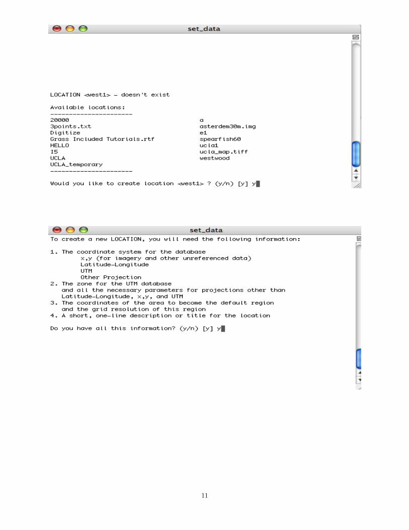
• Before we begin using the GRASS commnands we will first learn how to create a new LOCATION.There are three ways to create a new location (by clicking on Georeferenced file, or EPSG codes,or Projection values as shown on the screenshot below. We will begin using the last one (Projectionvalues).
9

To create a new LOCATION using the last option, click on “Projection values”. This will take you tothe next window:
Suppose we want to create the LOCATION “west1”. Simply enter the name west1 next to LOCATION(as shown above) and hit return. Give a name to mapset (say, aaaaa). Then press ESC and thenENTER and follow the steps below as described by the screenshots...
10
11

Note: Here we choose the option “A” because we do not have any coordinates available at the moment.We choose a general non-georeferenced coordinate system x, y.
12

Note: Set the WEST EDGE and SOUTH EDGE values to zero, and enter for NORTH EDGE thenumber of rows and for EAST EDGE the number of columns. The next page explains what the numberof columns and rows are. For the GRID RESOLUTION you can choose 1, because the units are pixels.See next page...
13

Note: To find the number of rows and columns: If you are using a MAC computer, click on Applekey+i. If you are using a PC computer, do right click and select properties. The example below showsthe map of South America and the corresponding number of rows and columns. The number of rowsand columns that we enter (see previous snapshots) should cover at least the size of the map thatwe want to import, It can be defined larger than needed. This will not use extra memory since thememory used depends only on the actual size of the file imported.
14

The map we want to import in GRASS for this tutorial is the following:
15

16

So far, we have created a new LOCATION (west1) and a new MAPSET (aaaaa). Also, GRASS hascreated automatically the PERMANENT mapset. See next snapshot of the GRASS startup screen.
17

We can now create new MAPSETs by first selecting the LOCATION we want (here, west1) and thenentering the MAPSET’s name in the box below “Create new mapset in selected location”. Say, wewant to create a new mapset named aa1. Here is the output:
18

To enter GRASS, we select the mapset “aaaaa” and click on “Enter GRASS”. This will take you tothe following:
Note: The upper left window as shown in this snapshot, is the terminal “GRASS Command Window”.This is the window where you type your commands (more will follow soon...). The upper right windowit is called the “GIS Manager” and the window on the lower right is the “Map Display” window. Thewindow on the lower left contains messages after we run a GRASS command. The last three windowsare linked together. The “GRASS Command Window” can also display maps, etc., but we will haveto open a monitor first. So, there are two ways to work with GRASS data: Either through the GRASSCommand Window and a monitor, or with the other three windows as shown in the snapshot above.
19

Import and display raster data
Suppose we want to import and display the map “snow.jpg”, which located under
~/grass/snow.jpg
On the terminal GRASS Window Command type the following commands (in the snapshots below,we can see the output of these commands):
GRASS 6.3.cvs (w1):~ > r.in.gdal in=~/grass/snow.jpg out=snowProjection of input dataset and current location appear to match.Proceeding with import...100%100%100%GRASS 6.3.cvs (w1):~ > g.list rast
----------------------------------------------<raster> files available in mapset <a3>:snow.blue snow.green snow.red
----------------------------------------------GRASS 6.3.cvs (w1):~ > d.mon x0using default visual which is TrueColorncolors: 16777216Graphics driver [x0] startedGRASS 6.3.cvs (w1):~ > d.rast snow.green100%GRASS 6.3.cvs (w1):~ > r.compositeGRASS 6.3.cvs (w1):~ > d.rast snow3100%
20

Here is what each one of the previous GRASS commands does:
> r.in.gdal in=~/grass/snow.jpg out=snowImports the map snow.jpg and gives it the name “snow”.
> g.list rastLists all the maps created by GRASS. Here we have snow.blue, snow.green, snow.red.
> d.mon x0Opens a new window in order to display the map.
> d.rast snow.greenDisplays the map snow.green (see screenshot below).
> r.compositeOpens a new window in order to combine the three maps (see screenshot below).
> d.rast snow3Displays the map with the three colors combined.
Map snow.green is displayed:
Note: GRASS uses the RGB color model. In this model the three colors (red, green, blue) are usedin varying intensities to produce other colors. The intensity of each of the three colors (red, blue,green) is measured on a scale from 0-255 (0 represents no color, 255 represents maximum intensity).For example, the black color can be obtained when R = 0, B = 0, G = 0, etc.
21

Combine snow.blue, snow.green, snow.red into a map named snow3:
22

The output:
23

The new map:
> d.rast snow3
24

Another way to display maps is through the GIS Manager and the Map Display window. This is shownbelow in the 4 snapshots. First click on the raster icon below “Config”.
Then click on “Base map:” below and select the raster map snow3.
25

And looks like this:
And you can display the map at the Map Display window (click on the upper left icon):
26

The g.region command: Managing map regions and resolutions
• To change the region, resolution, and boundaries of the map the g.region command is used with thefollowing flags and options: -d, -p, -l, -e, -c, -o, -dp, res, n, s, w, e, save.
-p Print region-d Gives Default region-l Gives Print lat/long-e Gives extent of the region-c Gives center coordinatessave Saves the current regionres= Changes resolutionnsres= Changes resolution n-sewres= Changes resolution e-wn= Changes the north extents= Changes the south extente= Changes the east extentw= Changes the west extent
Here are some examples:
• Here is how we can get the current region numbers:
GRASS 6.3.cvs (west1):~ > g.region -pec rast=snow3projection: 0 (x,y)zone: 0north: 1878south: 0west: 0east: 900nsres: 1ewres: 1rows: 1878cols: 900cells: 1690200north-south extent: 1878.000000east-west extent: 900.000000center easting: 450.000000center northing: 939.000000GRASS 6.3.cvs (west1):~ >
27
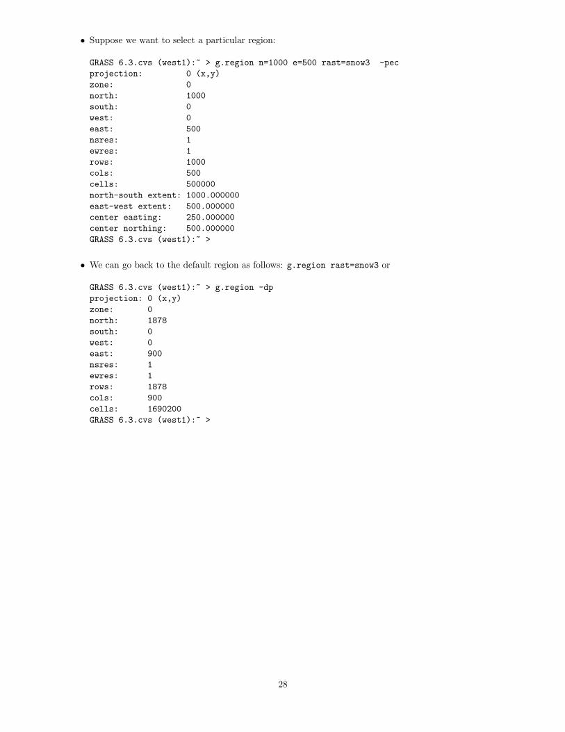
• Suppose we want to select a particular region:
GRASS 6.3.cvs (west1):~ > g.region n=1000 e=500 rast=snow3 -pecprojection: 0 (x,y)zone: 0north: 1000south: 0west: 0east: 500nsres: 1ewres: 1rows: 1000cols: 500cells: 500000north-south extent: 1000.000000east-west extent: 500.000000center easting: 250.000000center northing: 500.000000GRASS 6.3.cvs (west1):~ >
• We can go back to the default region as follows: g.region rast=snow3 or
GRASS 6.3.cvs (west1):~ > g.region -dpprojection: 0 (x,y)zone: 0north: 1878south: 0west: 0east: 900nsres: 1ewres: 1rows: 1878cols: 900cells: 1690200GRASS 6.3.cvs (west1):~ >
28

• We can change the resolution of the region:
GRASS 6.3.cvs (west1):~ > g.region nsres=2 ewres=2 rast=snow3 -pecprojection: 0 (x,y)zone: 0north: 1878south: 0west: 0east: 900nsres: 2ewres: 2rows: 939cols: 450cells: 422550north-south extent: 1878.000000east-west extent: 900.000000center easting: 450.000000center northing: 939.000000GRASS 6.3.cvs (west1):~ >
• There are many options to set the region. Here is another one: The north and east extent are given interms of the south and west. The result will be a region on the south-west corner of the current region.
GRASS 6.3.cvs (west1):~ > g.region n=s+500 e=w+500 rast=snow3 -pprojection: 0 (x,y)zone: 0north: 500south: 0west: 500east: 900nsres: 1ewres: 1rows: 500cols: 400cells: 200000north-south extent: 500.000000east-west extent: 400.000000center easting: 700.000000center northing: 250.000000GRASS 6.3.cvs (west1):~ >
• The changed region can be saved using g.region -s, but this must be done from the PERMANENTMAPSET.
In the next pages we will explore how GRASS and the package gstat of R can be used to analyze spatial data.The method of spatial prediction called kriging will be used. The installation of the R/GRASS interface canbe done by a single command:
install.packages("spgrass6", "gstat", type="source", dependencies=TRUE)
29

Spatial data analysis with GRASS and R - Exampe
We will use the data from the Walker Lake of Nevada (variable v - see figure below). The variable V is measured inparts per million (ppm) at the Walker Lake area in the state of Nevada (from An Introduction to Applied Geostatisticsby Issaks, E., and Srivastava, R. M. (1989)).
You can access the data at:
a1 <- read.table("http://www.stat.ucla.edu/~nchristo/statistics_c173_c273/
walker_lake_v.txt", header=TRUE)
First we need to create a new location that will hold these data. You can name it w13, and also create a mapseta1 . Read the data first in R to find the north-south and east-west extend of the tegion. To create the location inGRASS we use projection values and choose x, y coordinates. The minimum value of x is 8 and its maximum 251. Theminimum value of y is 8 and its maximum 291. Therefore define the location as follows:North: 252South: 7West: 7East: 292and give resolution 1 to both N to S and E to W.You are done!
Enter GRASS through the location w13 and mapset a1. Once you are at the GRASS prompt the data can be accessedand imported using the v.in.ascii command. Give an output name v in. See the snapshots of the v.in.ascii
module below:
30

Define the columns of the data set:
Once you have imported the file, display the points (first open a monitor window, and then type d.vect v in). Youcan customize the size and the type of the symbols as shown below. For more information type d.vect help. Herewe used:
GRASS 6.3.cvs (w13):~ > d.vect v_in size=5 icon=basic/circle
to get the following plot:
31
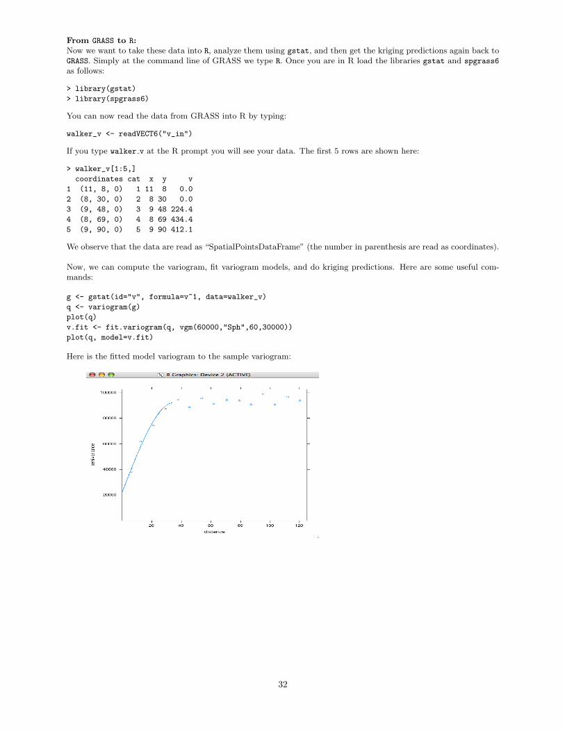
From GRASS to R:Now we want to take these data into R, analyze them using gstat, and then get the kriging predictions again back toGRASS. Simply at the command line of GRASS we type R. Once you are in R load the libraries gstat and spgrass6
as follows:
> library(gstat)
> library(spgrass6)
You can now read the data from GRASS into R by typing:
walker_v <- readVECT6("v_in")
If you type walker v at the R prompt you will see your data. The first 5 rows are shown here:
> walker_v[1:5,]
coordinates cat x y v
1 (11, 8, 0) 1 11 8 0.0
2 (8, 30, 0) 2 8 30 0.0
3 (9, 48, 0) 3 9 48 224.4
4 (8, 69, 0) 4 8 69 434.4
5 (9, 90, 0) 5 9 90 412.1
We observe that the data are read as “SpatialPointsDataFrame” (the number in parenthesis are read as coordinates).
Now, we can compute the variogram, fit variogram models, and do kriging predictions. Here are some useful com-mands:
g <- gstat(id="v", formula=v~1, data=walker_v)
q <- variogram(g)
plot(q)
v.fit <- fit.variogram(q, vgm(60000,"Sph",60,30000))
plot(q, model=v.fit)
Here is the fitted model variogram to the sample variogram:
32

We create now the grid for the kriging predictions:
x.range <- range(walker_v$x)
x.range
[1] 8 251
y.range <- range(walker_v$y)
y.range
[1] 8 291
grd <- expand.grid(x=seq(from=x.range[1], to=x.range[2], by=1),
y=seq(from=y.range[1], to=y.range[2], by=1) )
class(grd)
coordinates(grd) <- ~x+y
gridded(grd) <- TRUE
class(grd)
plot(grd, cex=0.5)
points(walker_v, pch=1, col="green", cex=0.7)
The grid with the data points:
Now we update the gstat object and perform ordinary kriging as follows:
g <- gstat(g, id="v", model=v.fit ) #Update object g.
v_ok <- predict.gstat(g, model=v.fit, newdata=grd)
#Or using the krige function:
v_ok <- krige(id="v", v~1, walker_v, grd, model = v.fit)
names(v_ok)
v_ok$v.pred
v_ok$v.var
33

From R back to GRASS:Now we can save the predicted values and their variances as follows:
> writeRAST6(v_ok, "v_pred", zcol="v.pred")
Projection of input dataset and current location appear to match.
Proceeding with import...
100%
> writeRAST6(v_ok, "v_var", zcol="v.var")
Projection of input dataset and current location appear to match.
Proceeding with import...
100%
Type q() to leave R and go back to GRASS.In GRASS open a new monitor to display the maps.
d.mon x0
d.rast v_pred
d.rast v_var
You can also create a vector map that displays the contours with the following command:
GRASS 6.3.cvs (w13):~ > r.contour v_pred out=v_pred_cont step=50
Reading data:
100%
Range of data: min = -78.295837 max = 1528.099976
Range of levels: min = 0.000000 max = 1500.000000
Displacing data:
100%
Total levels: 31
WARNING: 85 crossings founds
Building topology ...
652 primitives registered
Building areas: 100%
0 areas built
0 isles built
Attaching islands:
Attaching centroids: 100%
Topology was built.
Number of nodes : 680
Number of primitives: 652
Number of points : 0
Number of lines : 652
Number of boundaries: 0
Number of centroids : 0
Number of areas : 0
Number of isles : 0
r.contour complete.
Here is the raster map with the contours:
GRASS 6.3.cvs (w13):~ > d.vect v_pred_cont
34

A very interesting and useful tool for a 3D visualization in GRASS is the nviz tool. At the GRASS prompt you type
GRASS 6.3.cvs (w13):~ > nviz v_pred
This command will display the following:
If you want to display the data points click on “Visualize” and access the data points through “Vector Points”.
Using the available options you can control different parameters. You can also save this display by clicking on “File”and then on “Save image as” and you can save it as a TIFF file.
Exercise:Repeat the above using the data walker lake u.txt.
35

Spatial data analysis with GRASS and R - Exampe
We will use the Wolfcamp data from Texas (see Cressie (1993, pp. 212-214). The U.S. Department of Energyproposed (in the 1980s) a nuclear waste site to be in Deaf Smith County in Texas (bordering New Mexico). Thecontamination of the aquifer was a concern, and therefore the piezometric-head data were obtained at 85 locationsby drilling a narrow pipe through the aquifer. The measures are in feet above sea level. See figure below for thelocation (Texas panhandle):
First we need to create a new location that will hold these data. You can name it wf, and also create a mapset a1 .Read the data first in R to find the north-south and east-west extend of the region. To create the location in GRASS
we use projection values and choose x, y coordinates. The minimum value of x is -145.2 and its maximum 112.8. Theminimum value of y is 9.4 and its maximum 184.8. Therefore define the location as follows:North: 186South: 8West: -144East: 114and give resolution 1 to both N to S and E to W.You are done!
Enter GRASS through the location wf and mapset a1. Once you are at the GRASS prompt access the ascii filewolfcamp.txt using the v.in.ascii command. Give an output name wolfcamp in. See the snapshots of thev.in.ascii module below:
36

Define the columns of the data set:
Once you have imported the file, display the points (first open a monitor window, and then type d.vect wolfcamp in).You can customize the size and the type of the symbols as shown below. For more information type d.vect help.Here we used:
GRASS 6.3.cvs (wf):~ > d.vect wolfcamp_in size=5 icon=basic/circle
to get the following plot:
37

From GRASS to R:Now we want to take these data into R, analyze them using gstat, and then get the kriging predictions again back toGRASS. Simply at the command line of GRASS we type R. Once you are in R load the libraries gstat and spgrass6
as follows:
> library(gstat)
> library(spgrass6)
You can now read the data from GRASS into R by typing:
a <- readVECT6("wolfcamp_in")
If you type a at the R prompt you will see your data. The first 5 rows are shown here:
> a[1:5,]
coordinates cat x y level
1 (42.8, 127.6, 0) 1 42.8 127.6 1464
2 (-27.4, 90.8, 0) 2 -27.4 90.8 2553
3 (-1.2, 84.9, 0) 3 -1.2 84.9 2158
4 (-18.6, 76.5, 0) 4 -18.6 76.5 2455
5 (96.5, 64.6, 0) 5 96.5 64.6 1756
We observe that the data are read as “SpatialPointsDataFrame” (the number in parenthesis are read as coordinates).Now, we can compute variograms, fit variogram models, and do kriging predictions. For this example we use universalkriging (see handout on universal kriging). Here are some useful commands:
g <- gstat(id="level", formula = level~x+y, data = a)
q <- variogram(g)
plot(q)
v.fit <- fit.variogram(q, vgm(30000,"Sph",60,10000))
plot(q, model=v.fit)
> v.fit
model psill range
1 Nug 9959.434 0.00000
2 Sph 33852.314 66.08075
Here is the fitted model variogram to the sample variogram:
38

We create now the grid for the kriging predictions:
> x.range <- as.integer(range(a$x))
> x.range
[1] -145 112
> y.range <- as.integer(range(a$y))
> y.range
[1] 9 184
grd <- expand.grid(x=seq(from=x.range[1], to=x.range[2], by=1),
y=seq(from=y.range[1], to=y.range[2], by=1))
class(grd)
coordinates(grd) <- ~x+y
gridded(grd) <- TRUE
class(grd)
plot(grd, cex=0.5)
points(a, pch=1, col="green", cex=0.9)
The grid with the data points:
39
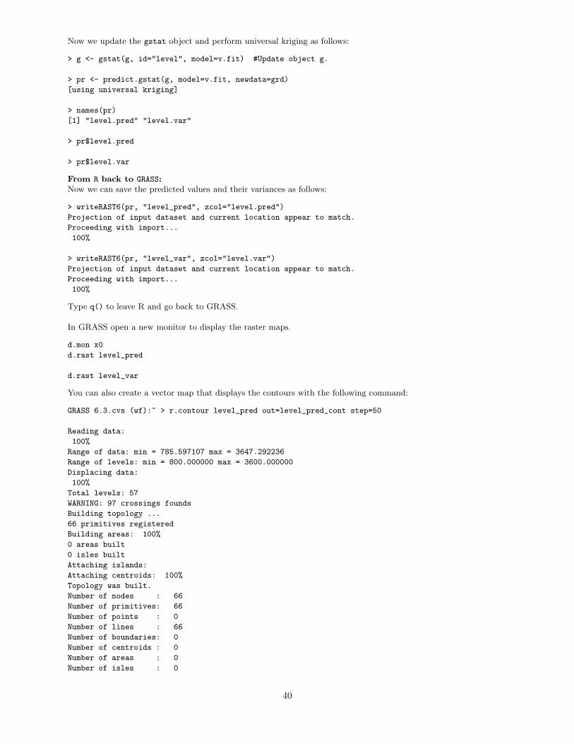
Now we update the gstat object and perform universal kriging as follows:
> g <- gstat(g, id="level", model=v.fit) #Update object g.
> pr <- predict.gstat(g, model=v.fit, newdata=grd)
[using universal kriging]
> names(pr)
[1] "level.pred" "level.var"
> pr$level.pred
> pr$level.var
From R back to GRASS:Now we can save the predicted values and their variances as follows:
> writeRAST6(pr, "level_pred", zcol="level.pred")
Projection of input dataset and current location appear to match.
Proceeding with import...
100%
> writeRAST6(pr, "level_var", zcol="level.var")
Projection of input dataset and current location appear to match.
Proceeding with import...
100%
Type q() to leave R and go back to GRASS.
In GRASS open a new monitor to display the raster maps.
d.mon x0
d.rast level_pred
d.rast level_var
You can also create a vector map that displays the contours with the following command:
GRASS 6.3.cvs (wf):~ > r.contour level_pred out=level_pred_cont step=50
Reading data:
100%
Range of data: min = 785.597107 max = 3647.292236
Range of levels: min = 800.000000 max = 3600.000000
Displacing data:
100%
Total levels: 57
WARNING: 97 crossings founds
Building topology ...
66 primitives registered
Building areas: 100%
0 areas built
0 isles built
Attaching islands:
Attaching centroids: 100%
Topology was built.
Number of nodes : 66
Number of primitives: 66
Number of points : 0
Number of lines : 66
Number of boundaries: 0
Number of centroids : 0
Number of areas : 0
Number of isles : 0
40

r.contour complete.
Here is the raster map with the contours and the data points:
GRASS 6.3.cvs (wf):~ > d.rast level_pred
100%
GRASS 6.3.cvs (wf):~ > d.vect level_pred_cont
GRASS 6.3.cvs (wf):~ > d.vect wolfcamp_in size=5 icon=basic/circle
41

A very interesting and useful tool for a 3D visualization in GRASS is the nviz tool. At the GRASS prompt you type
GRASS 6.3.cvs (wf):~ > nviz level_pred
This command will display the following:
If you want to display the data points click on “Visualize” and access the data points through “Vector Points”. Also,using the options “perspective”, “z-exag”, and “height” we get the following three-dimensional view plot from thenortheast corner.
Using the available options under “Appearance” we can change the colors, add text to the plot, add fringes, etc. Youcan also save this display by clicking on “File” and then on “Save image as” and you can save it as a TIFF file.
42
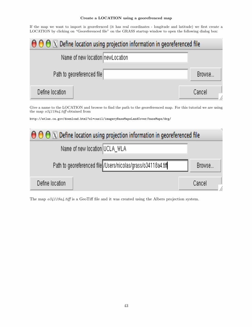
Create a LOCATION using a georefrenced map
If the map we want to import is georefernced (it has real coordinates - longitude and latitude) we first create aLOCATION by clicking on “Georeferenced file” on the GRASS startup window to open the following dialog box:
Give a name to the LOCATION and browse to find the path to the georeferenced map. For this tutorial we are usingthe map o34118a4.tiff obtained from
http://atlas.ca.gov/download.html?sl=casil/imageryBaseMapsLandCover/baseMaps/drg/
The map o34118a4.tiff is a GeoTiff file and it was created using the Albers projection system.
43

We have created a new LOCATION named UCLA WLA as shown on the GRASS startup screen below:
We observe that the PERMANENT mapset was created automatically by GRASS, but let’s create and enterGRASS through a mapset named ucla1:
44

At the command window we read the file, list the available raster maps (here there is only one - ucla), andopen a monitor to display the map:
GRASS 6.3.cvs (UCLA_WLA):~ > r.in.gdal in=~/grass/o34118a4.tiff out=uclaProjection of input dataset and current location appear to match.Proceeding with import...100%GRASS 6.3.cvs (UCLA_WLA):~ > g.list rast----------------------------------------------<raster> files available in mapset <ucla1>:ucla
----------------------------------------------GRASS 6.3.cvs (UCLA_WLA):~ > d.mon x0using default visual which is TrueColorncolors: 16777216Graphics driver [x0] startedGRASS 6.3.cvs (UCLA_WLA):~ > d.rast ucla100%GRASS 6.3.cvs (UCLA_WLA):~ >
Here is the map displayed through the monitor x0:
Another way of course to display the map is through the GIS Manager.
45

Let’s check the region for this map using the g.region command:
GRASS 6.3.cvs (UCLA_WLA):~ > g.region -pecprojection: 99 (Albers Equal Area)zone: 0datum: nad83ellipsoid: grs80north: -431016.92261189south: -445071.36291951west: 138267.95234148east: 150034.7091132nsres: 1.52715857ewres: 1.52715857rows: 9203cols: 7705cells: 70909115north-south extent: 14054.440308east-west extent: 11766.756772center easting: 144151.330727center northing: -438044.142766GRASS 6.3.cvs (UCLA_WLA):~ >
We have the following:The projection used for this map is Albers Equal Area, datum is nad83, and ellipsoid is grs80. The numbers
north: -431016.92261189south: -445071.36291951west: 138267.95234148east: 150034.7091132
define the extent of our region. The resolution is 1.52715857 on both n-s and e-s directions. From these wecan get the number of rows and columns using the following calculation:
Number of rows=(445071.36291951-431016.92261189)/1.52715857=9203andNumber of columns=(150034.7091132-138267.95234148)/1.52715857=7705
The resolution can be changed, as discussed in the previous handout using the command g.region with theoptions nsres and ewres. For example
GRASS 6.3.cvs (UCLA_WLA):~ > g.region nsres=2 ewres=2
46

If we want to see the longitude and latitude for this region we use the flag �-l:
GRASS 6.3.cvs (UCLA_WLA):~ > g.region -lpecprojection: 99 (Albers Equal Area)zone: 0datum: nad83ellipsoid: grs80north: -431016.92261189south: -445071.36291951west: 138267.95234148east: 150034.7091132nsres: 1.52715857ewres: 1.52715857rows: 9203cols: 7705cells: 70909115north-west corner: long: 118:30:03.164016W lat: 34:07:36.185959Nnorth-east corner: long: 118:22:23.973857W lat: 34:07:29.891711Nsouth-east corner: long: 118:22:33.369749W lat: 33:59:53.850963Nsouth-west corner: long: 118:30:11.8234W lat: 34:00:00.135983Ncenter longitude: 118:26:18.082755Wcenter latitude: 34:03:45.016154Nnorth-south extent: 14054.440308east-west extent: 11766.756772center easting: 144151.330727center northing: -438044.142766GRASS 6.3.cvs (UCLA_WLA):~ >
47

Connecting more than one quadrangles together (by Jan de Leeuw)
Again we obtained 6 quadrangles as shown on the map below from
http://atlas.ca.gov/casil/imageryBaseMapsLandCover/baseMaps/drg/7.5_minute_series_albers_nad83_untrimmed/
http://atlas.ca.gov/casil/imageryBaseMapsLandCover/baseMaps/drg/7.5_minute_series_albers_nad83_untrimmed/34118/
We want to import and connect the 6 quadrangles named:Beverly Hills, Van Nuys, Canoga Park, Calabasas, Malibu Beach, and Topanga. The file names of thesequadrangles are 034118a4, 034118b4, 034118b5, 034118b6, 034118a6, 034118a5.
48

First let’s exit GRASS and enter again through UCLA WLA and the PERMANENT mapset (we will seewhy...). We then use r.in.gdal to read these files. At the command window we type the following one at atime.
r.in.gdal in=~/grass/o34118a4.tiff out=Ar.in.gdal in=~/grass/o34118b4.tiff out=Br.in.gdal in=~/grass/o34118b5.tiff out=Cr.in.gdal in=~/grass/o34118b6.tiff out=Dr.in.gdal in=~/grass/o34118a6.tiff out=Er.in.gdal in=~/grass/o34118a5.tiff out=F
And here is what we have...
GRASS 6.3.cvs (UCLA_WLA):~ > g.list rast----------------------------------------------<raster> files available in mapset <PERMANENT>:A B C D E F
----------------------------------------------GRASS 6.3.cvs (UCLA_WLA):~ >
We will now create and save the new region that will hold all 6 maps:
GRASS 6.3.cvs (UCLA_WLA):~ > g.region -s rast=A,B,C,D,E,FGRASS 6.3.cvs (UCLA_WLA):~ > g.region -pprojection: 99 (Albers Equal Area)zone: 0datum: nad83ellipsoid: grs80north: -417152.28930665south: -445407.37680891west: 115026.92199555east: 150034.7091132nsres: 1.52713693ewres: 1.52719047rows: 18502cols: 22923cells: 424121346GRASS 6.3.cvs (UCLA_WLA):~ >
49

We then open a monitor to display the maps. We type the following commands one at a time, and we alsouse the flag -o which stands for overlay:
d.rast -o map=Ad.rast -o map=Bd.rast -o map=Cd.rast -o map=Dd.rast -o map=Ed.rast -o map=F
The 6 maps are displayed one by one in the monitor and finally we get the picture below:
We can improve the result by removing the spaces between the quadrangles. Also, we want to create a newmap that contains all these 6 quadrangles. This is done with the following commands:
50

GRASS 6.3.cvs (UCLA_WLA):~ > r.series in=A,B,C,D,E,F out=wla method=maximumPercent complete ...100%GRASS 6.3.cvs (UCLA_WLA):~ > g.list rast----------------------------------------------<raster> files available in mapset <PERMANENT>:A B C D E F wla
----------------------------------------------GRASS 6.3.cvs (UCLA_WLA):~ >
We have used the command r.series with the option method=maximum which takes the maximum of allpixels in the region over all rasters. The input maps are the 6 quadrangles and we named the output mapwla.
We also want to keep the original colors (from A, B, C, D, E, F). We can choose any one of the 6 maps tobe the base color for our newly created map wla. Here is the command:
GRASS 6.3.cvs (UCLA_WLA):~ > r.colors map=wla rast=AColor table for [wla] set to AGRASS 6.3.cvs (UCLA_WLA):~ >
Note: Other options for method=average: average valuecount: count of non-NULL cellsmedian: median valuemode: most frequently occuring valueminimum: lowest valuestddev: standard deviationsum: sum of valuesetc.
51
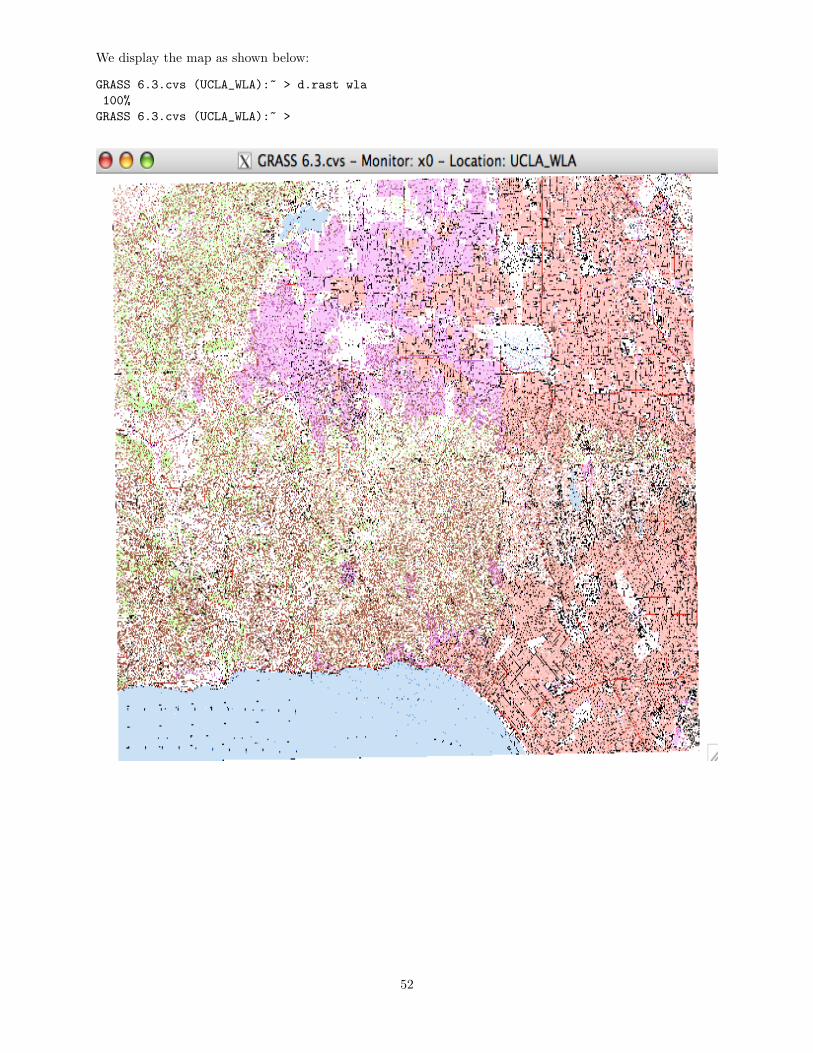
We display the map as shown below:
GRASS 6.3.cvs (UCLA_WLA):~ > d.rast wla100%GRASS 6.3.cvs (UCLA_WLA):~ >
52
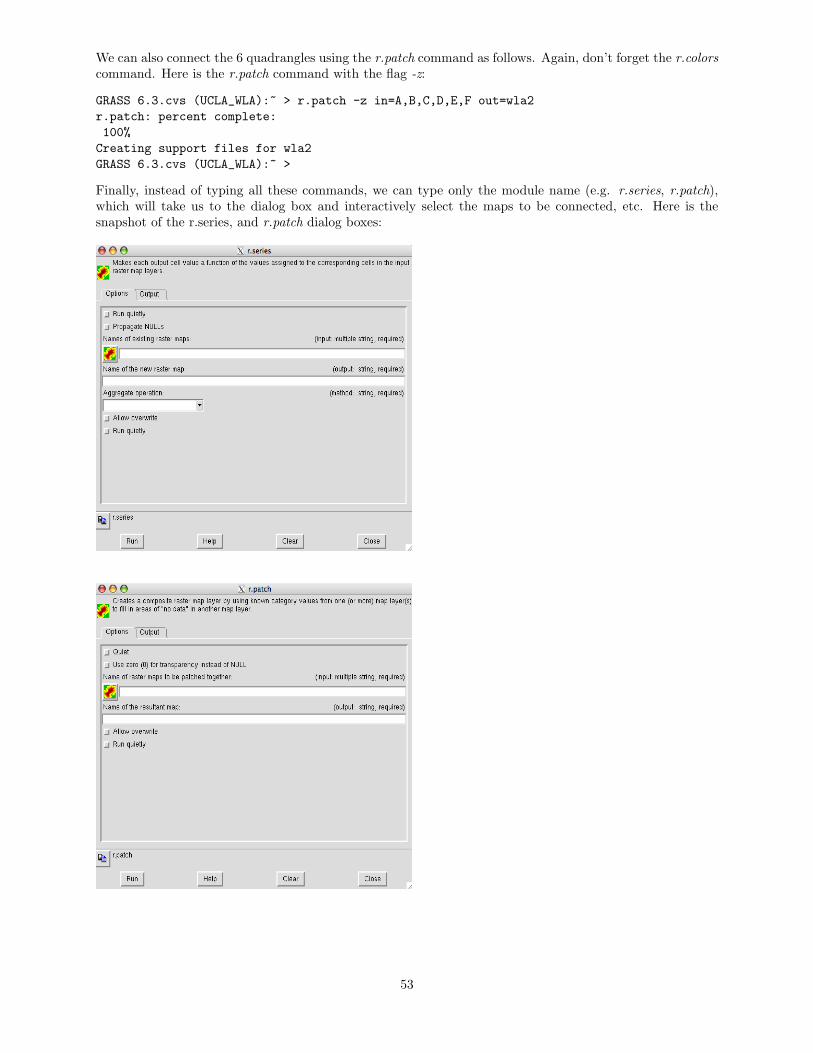
We can also connect the 6 quadrangles using the r.patch command as follows. Again, don’t forget the r.colorscommand. Here is the r.patch command with the flag -z:
GRASS 6.3.cvs (UCLA_WLA):~ > r.patch -z in=A,B,C,D,E,F out=wla2r.patch: percent complete:100%Creating support files for wla2GRASS 6.3.cvs (UCLA_WLA):~ >
Finally, instead of typing all these commands, we can type only the module name (e.g. r.series, r.patch),which will take us to the dialog box and interactively select the maps to be connected, etc. Here is thesnapshot of the r.series, and r.patch dialog boxes:
53

More commands...To rename a raster map we use g.rename rast=old mapname, new mapname.To remove a raster map we use g.remove rast=mapname.To access raster maps in other mapsets other than the current mapset: Suppose you are in mapset ucla1 ofthe location UCLA WLA but you want to display the map wla from the PERMANENT mapset. You cantype:
GRASS 6.3.cvs (UCLA_WLA):~ > d.rast wla@PERMANENT100%GRASS 6.3.cvs (UCLA_WLA):~ >
To export a map as a TIFF file you use:
GRASS 6.3.cvs (UCLA_WLA):~ > r.out.tiff in=ucla13out=/Users/nicolas/Desktop/ucla_area
100%r.out.tiff complete.GRASS 6.3.cvs (UCLA_WLA):~ >
You can also use the dialog box after you type the command r.out.tiff.
Note: GRASS can export raster data to more than 20 different formats using the r.out.gdal module. Someof them are GTiff, PNG, JPEG, GIF, BMP, etc.
54

More on raster maps
Creating a new LOCATION using the r.in.gdal command:The command r.in.gdal is another way to create a location. Suppose that LOCATION west1 already exists.We enter GRASS through west1 and mapset aaaaa. We are at the command window as follows:
Welcome to GRASS 6.3.cvs (2007)GRASS homepage: http://grass.itc.it/This version running thru: Bash Shell (/bin/bash)Help is available with the command: g.manual -iSee the licence terms with: g.version -cIf required, restart the graphical user interface with: gis.mWhen ready to quit enter: exitGRASS 6.3.cvs (west1):~ >
To create a new location at the command line we type:
GRASS 6.3.cvs (west1):~ > r.in.gdal ~/grass/snow.jpg location=west1a> out=snow100%100%100%GRASS 6.3.cvs (west1):~ >
What happened here? r.in.gdal reads the file snow.jpg from the home directory ∼/grass, gives the outputname snow and creates a new location names west1a. The coordinates of the new location west1a will be thesame as with the location west1. To check what we just did, exit from GRASS and go back to the startupscreen:
55
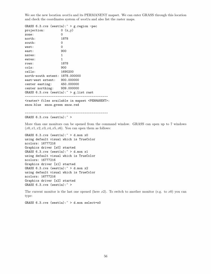
We see the new location west1a and its PERMANENT mapset. We can enter GRASS through this locationand check the coordinates system of west1a and also list the raster maps.
GRASS 6.3.cvs (west1a):~ > g.region -pecprojection: 0 (x,y)zone: 0north: 1878south: 0west: 0east: 900nsres: 1ewres: 1rows: 1878cols: 900cells: 1690200north-south extent: 1878.000000east-west extent: 900.000000center easting: 450.000000center northing: 939.000000GRASS 6.3.cvs (west1a):~ > g.list rast----------------------------------------------<raster> files available in mapset <PERMANENT>:snow.blue snow.green snow.red
----------------------------------------------GRASS 6.3.cvs (west1a):~ >
More than one monitors can be opened from the command window. GRASS can open up to 7 windows(x0, x1, x2, x3, x4, x5, x6). You can open them as follows:
GRASS 6.3.cvs (west1a):~ > d.mon x0using default visual which is TrueColorncolors: 16777216Graphics driver [x0] startedGRASS 6.3.cvs (west1a):~ > d.mon x1using default visual which is TrueColorncolors: 16777216Graphics driver [x1] startedGRASS 6.3.cvs (west1a):~ > d.mon x2using default visual which is TrueColorncolors: 16777216Graphics driver [x2] startedGRASS 6.3.cvs (west1a):~ >
The current monitor is the last one opened (here x2). To switch to another monitor (e.g. to x0) you cantype:
GRASS 6.3.cvs (west1a):~ > d.mon select=x0
56