university of castilla-la mancha vibration - ruidera
TRANSCRIPT
UNIVERSITY OF CASTILLA-LA MANCHA
Escuela Tecnica Superior de Ingenieros Industriales
Departamento de Ingenierıa Electrica, Electronica,
Automatica y de Comunicaciones
Vibration Control Strategies for a
Very Lightweight One Degree-Of-Freedom
Flexible Arm Built with Composite Material
Ph. D. Thesis
SupervisorVicente Feliu Batlle
AuthorFrancisco Ramos de la Flor
Ciudad Real, 2009


”If you are out to describe the truth, leave elegance to the tailor.”
Albert Einstein.

Acknowledgements/Agradecimientos
Ha sido un largo camino, sembrado con dificultades pero tambien con numerosas
alegrıas y experiencias de las que completan a una persona y hacen que se sienta
viva. He conocido mucha gente buena (de la mala por suerte no me acuerdo) que me
ha ayudado, apoyado, animado, escuchado, y tantos otros -ados, y a la que quiero
agradecer su tiempo, su esfuerzo y, en la mayor parte de casos, su amistad.
En primer lugar debo agradecer la posibilidad de haber realizado esta Tesis a mi
director, el Profesor Vicente Feliu Batlle, quien me enseno el camino de baldosas amar-
illas de la investigacion cientıfica y me ha guiado por el con una paciencia que roza
lo ilimitado. Del mismo modo, agradezco a la Junta de Comunidades de Castilla-La
Mancha la financiacion recibida en forma de beca predoctoral puesto que sin dicho
apoyo no hubiese podido terminar estos estudios.
Tambien tengo que dar las gracias a mis antes profesores, a los que ahora llamo
companeros e incluso amigos: Luis Sanchez, Pedro Roncero, Jose Andres Somolinos y,
especialmente, a Daniel Cortazar, quien ha intentado hacer de mı un buen docente,
ademas de regalarme valiosısimas ensenanzas acerca de la vida.
Y ahora viene la parte mas extensa, porque he tenido muchos y muy buenos
companeros durante esta etapa y se lo quiero agradecer aunque solo sea con una lınea.
A Rafa, porque fue el primero que recorrio el camino conmigo y despues de tantos
anos se que aun puedo confiar en el, y a Ismael, el hombre que siempre suma, quien
incluso me ha abierto las puertas de su casa cuando me ha hecho falta, no me olvido
de ello. A Fernando, quien me ha hecho sonreır en momentos muy difıciles y siempre
tiene la solucion para el problema, da igual cual sea el problema. A Virginia, que
ha compartido mil y un cafes conmigo aportando ideas, animandome y dandome la
calma cuando me he encontrado mal. A Juanra, quien ha escuchado pacientemente
5

todas mis historias y mis histerias y se ha reıdo con todos mis chistes malos: eso es
amistad. Y especialmente a Emiliano, el de Badaho, mi hermano pacense, que se ha
convertido en una parte muy importante de mı. Nunca antes haba encontrado una
persona tan dispuesta a ayudar y tan sacrificada por los demas salvo mi madre. Y
hay mucha gente mas que lleva tiempo por aquı: Jose Antonio, Elisa, Pedro, Gabi,
Johnny, Ivan, Andres... O que hace menos que llego: Raul, Vıctor Hugo, Xavi, Salva,
Juanmi, Carlos... Gracias a todos. Siento que parezca la guıa de telefonos, pero aun
ası se me olvidara gente. Como se me olvidaba Shigueo, el brasileno mas exotico que
nunca conocere y el peor jugador de futbol, muito obrigado por sua amizade.
I will not miss my stay at University College Dublin, and all the fantastic people
I met there. First of them, my tutor, Dr. William J. O’Connor, who received me
with open hands, a big smile and a handful of ideas to solve the problem I came up
with. He always had time to help me to absorb his wave control ideas: “Engage brain,
Fran”. Also the lads at the office: Johhny, John, Barry and James for the laughs and
for repeating three times each joke so I could laugh with them. I will not forget to
Tang-Wen Yang, good colleague and better person. And finally, to David Joseph, not
nice at all, not even polite some times, but one of my best friends so far. I still keep
the Santa’s hat (without ball). It was great luck to find you, buachaill beag, and yes,
I know: You finished first!
En el aspecto personal, quiero agradecer a mis amigos que hayan aguantado, mejor
o peor, mi mal humor durante algunos periodos, ellos me han ayudado a “desfruncir”
el ceno. A Quiteria quiero agradecerle de corazon que haya sacrificado tanto (quiza
demasiado) por darme fuerzas en los momentos mas delicados para que llegase este
dıa, y pedirle perdon porque le ha tocado vivir lo peor de mı. Y como no, a mi familia,
que me ha apoyado todo el tiempo en las decisiones difıciles o incluso en las erroneas.
Gracias a mis sobrinas por sonreırme tanto y hacerme sonreır tanto a mı.
Esta Tesis ha necesitado muchos agradecimientos y falta el mas importante. A mi
madre, que me dio la vida hace ya muchos anos y no pasa un dıa sin que me la vuelva
a dar. Si el mundo estuviese lleno de personas como ella, serıa infinitamente mejor.
Ciudad Real,
Diciembre de 2009
Contents
1 Introduction 1
1.1 Preamble . . . . . . . . . . . . . . . . . . . . . . . . . . . . . . . . . . 1
1.1.1 Framework of the Thesis . . . . . . . . . . . . . . . . . . . . . . 1
1.1.2 Origins of the research group . . . . . . . . . . . . . . . . . . . 2
1.2 A brief history on flexible robotics . . . . . . . . . . . . . . . . . . . . . 3
1.2.1 Dawn: what if we make lighter manipulators? . . . . . . . . . . 3
1.2.2 Golden age: First devices, first controls . . . . . . . . . . . . . . 5
1.2.3 Flexible boom: have your own flexible robot! . . . . . . . . . . . 7
1.2.4 Next generation: the search for new applications . . . . . . . . . 9
1.3 Motivation . . . . . . . . . . . . . . . . . . . . . . . . . . . . . . . . . . 10
1.4 Objectives of the Thesis . . . . . . . . . . . . . . . . . . . . . . . . . . 11
1.5 Organization of the manuscript . . . . . . . . . . . . . . . . . . . . . . 11
2 Dynamic Models for Single-Link Flexible Arms 13
2.1 Generic description . . . . . . . . . . . . . . . . . . . . . . . . . . . . . 13
2.2 Actuator model . . . . . . . . . . . . . . . . . . . . . . . . . . . . . . . 15
2.3 Distributed masses model . . . . . . . . . . . . . . . . . . . . . . . . . 18
2.3.1 Solution of the Euler-Bernouilli Equation . . . . . . . . . . . . . 19
2.3.2 System model in space-state form . . . . . . . . . . . . . . . . . 21
2.4 Concentrated masses model . . . . . . . . . . . . . . . . . . . . . . . . 22
2.4.1 General model for an arbitrary number of masses . . . . . . . . 23
2.4.2 Model with negligible link mass and negligible payload rotational
inertia . . . . . . . . . . . . . . . . . . . . . . . . . . . . . . . . 26
ii Contents
2.4.3 Model with beam mass concentrated in its middle point and non-
negligible inertia at the payload . . . . . . . . . . . . . . . . . . 28
2.5 Nonlinear model for a very flexible manipulator with geometric non lin-
earities . . . . . . . . . . . . . . . . . . . . . . . . . . . . . . . . . . . . 31
2.5.1 On the Euler-Bernouilli beam . . . . . . . . . . . . . . . . . . . 33
2.5.2 General model . . . . . . . . . . . . . . . . . . . . . . . . . . . . 35
2.5.3 Linear model . . . . . . . . . . . . . . . . . . . . . . . . . . . . 35
2.5.4 Non linear model . . . . . . . . . . . . . . . . . . . . . . . . . . 36
2.6 Experimental platforms used for testing . . . . . . . . . . . . . . . . . . 38
2.6.1 Flexible arm with duraluminium link . . . . . . . . . . . . . . . 38
2.6.2 Flexible arm with composites link . . . . . . . . . . . . . . . . . 40
2.7 Note on the software used in the Thesis . . . . . . . . . . . . . . . . . . 45
3 Open loop control based on system inversion 47
3.1 Problem description . . . . . . . . . . . . . . . . . . . . . . . . . . . . . 47
3.1.1 Open loop control approach . . . . . . . . . . . . . . . . . . . . 48
3.1.2 Influence of trajectories . . . . . . . . . . . . . . . . . . . . . . . 49
3.2 System inversion based control scheme . . . . . . . . . . . . . . . . . . 50
3.2.1 Actuator control scheme . . . . . . . . . . . . . . . . . . . . . . 50
3.2.2 Noncausal dynamic inversion . . . . . . . . . . . . . . . . . . . . 52
3.3 Constrained trajectory design . . . . . . . . . . . . . . . . . . . . . . . 53
3.3.1 Control signal saturation . . . . . . . . . . . . . . . . . . . . . . 53
3.3.2 Motor controller tuning . . . . . . . . . . . . . . . . . . . . . . . 55
3.3.3 Trajectory definition . . . . . . . . . . . . . . . . . . . . . . . . 56
3.3.4 Kinematic limits . . . . . . . . . . . . . . . . . . . . . . . . . . 59
3.3.5 Physical limits . . . . . . . . . . . . . . . . . . . . . . . . . . . 61
3.4 Simulation results . . . . . . . . . . . . . . . . . . . . . . . . . . . . . . 64
3.4.1 Reference trajectory . . . . . . . . . . . . . . . . . . . . . . . . 65
3.4.2 Trajectory inversion . . . . . . . . . . . . . . . . . . . . . . . . 71
3.5 Experimental validation . . . . . . . . . . . . . . . . . . . . . . . . . . 72
3.5.1 Nominal case . . . . . . . . . . . . . . . . . . . . . . . . . . . . 72
3.5.2 Changes of the payload . . . . . . . . . . . . . . . . . . . . . . . 76
3.6 Summary and conclusions . . . . . . . . . . . . . . . . . . . . . . . . . 79
Contents iii
4 Robust control 81
4.1 Introduction . . . . . . . . . . . . . . . . . . . . . . . . . . . . . . . . . 81
4.2 PID controllers and their drawbacks . . . . . . . . . . . . . . . . . . . . 82
4.3 Robust controller . . . . . . . . . . . . . . . . . . . . . . . . . . . . . . 85
4.3.1 Outer loop . . . . . . . . . . . . . . . . . . . . . . . . . . . . . . 85
4.4 Robustness to payload changes . . . . . . . . . . . . . . . . . . . . . . 87
4.5 Robustness to small changes in system parameters . . . . . . . . . . . . 88
4.5.1 Robustness to errors in tuning the controller parameters . . . . 89
4.5.2 Robustness to changes of the motor parameters . . . . . . . . . 92
4.6 Simulation . . . . . . . . . . . . . . . . . . . . . . . . . . . . . . . . . . 94
4.6.1 Errors in the estimation of the bar stiffness . . . . . . . . . . . . 96
4.6.2 Errors in viscous friction estimation . . . . . . . . . . . . . . . . 101
4.6.3 Effects of noise in the feedback signal . . . . . . . . . . . . . . . 102
4.6.4 Effects of using a more complex dynamic model . . . . . . . . . 103
4.7 Experimental results . . . . . . . . . . . . . . . . . . . . . . . . . . . . 107
4.8 Conclusions . . . . . . . . . . . . . . . . . . . . . . . . . . . . . . . . . 108
5 Adaptive control 111
5.1 Introduction . . . . . . . . . . . . . . . . . . . . . . . . . . . . . . . . . 111
5.2 Previous experiences in adaptive control of flexible systems . . . . . . . 112
5.3 Payload estimation algorithm . . . . . . . . . . . . . . . . . . . . . . . 114
5.3.1 General payload estimator expression . . . . . . . . . . . . . . . 114
5.3.2 General lumped masses model . . . . . . . . . . . . . . . . . . . 116
5.3.3 Obtaining the gij transfer functions . . . . . . . . . . . . . . . . 118
5.4 Particular cases . . . . . . . . . . . . . . . . . . . . . . . . . . . . . . . 121
5.4.1 Beam with negligible mass . . . . . . . . . . . . . . . . . . . . . 121
5.4.2 Beam with its mass concentrated in a single point . . . . . . . . 122
5.4.3 Filtering the estimator . . . . . . . . . . . . . . . . . . . . . . . 123
5.5 Simulation results . . . . . . . . . . . . . . . . . . . . . . . . . . . . . . 125
5.5.1 Estimation algorithm . . . . . . . . . . . . . . . . . . . . . . . . 125
5.5.2 Application to adaptive control . . . . . . . . . . . . . . . . . . 133
5.6 Experimental validation . . . . . . . . . . . . . . . . . . . . . . . . . . 138
5.7 Summary and Conclusions . . . . . . . . . . . . . . . . . . . . . . . . . 141
iv Contents
6 Wave-based control 143
6.1 Introduction . . . . . . . . . . . . . . . . . . . . . . . . . . . . . . . . . 143
6.2 Wave-absorb theory fundamentals . . . . . . . . . . . . . . . . . . . . . 144
6.2.1 Simulating the behavior of an infinite chain of masses . . . . . . 145
6.3 Wave-absorb control scheme . . . . . . . . . . . . . . . . . . . . . . . . 146
6.3.1 Performance and robustness . . . . . . . . . . . . . . . . . . . . 149
6.4 WBC applied to a non-linear system . . . . . . . . . . . . . . . . . . . 149
6.5 Correcting the steady-state error . . . . . . . . . . . . . . . . . . . . . 153
6.5.1 Addition of a linear element . . . . . . . . . . . . . . . . . . . . 154
6.5.2 Performing a second movement . . . . . . . . . . . . . . . . . . 154
6.5.3 Force based redefinition of waves . . . . . . . . . . . . . . . . . 155
6.6 Experimental verification . . . . . . . . . . . . . . . . . . . . . . . . . . 160
6.6.1 Linear system . . . . . . . . . . . . . . . . . . . . . . . . . . . . 160
6.6.2 Non linear system . . . . . . . . . . . . . . . . . . . . . . . . . . 163
6.7 Conclusions . . . . . . . . . . . . . . . . . . . . . . . . . . . . . . . . . 166
7 Conclusions, contributions and suggested future research 167
7.1 Summary and conclusions . . . . . . . . . . . . . . . . . . . . . . . . . 167
7.2 Original contributions . . . . . . . . . . . . . . . . . . . . . . . . . . . 168
7.3 List of publications . . . . . . . . . . . . . . . . . . . . . . . . . . . . . 169
7.4 Open topics for future research . . . . . . . . . . . . . . . . . . . . . . 171
Bibliography 172
List of Figures
2.1 Scheme of a single dof flexible robot arm. . . . . . . . . . . . . . . . . . 14
2.2 Model for DC motor actuator. . . . . . . . . . . . . . . . . . . . . . . . 17
2.3 Scheme of a single dof flexible arm with distributed link mass . . . . . 20
2.4 Outline of a link represented by a finite number of point masses. . . . . 23
2.5 Outline of the negligible link mass and negligible payload inertia model 27
2.6 Outline of the model taking into account link mass and payload inertia 29
2.7 Large deflection of a one side clamped beam . . . . . . . . . . . . . . . 34
2.8 Dynamic deflection model . . . . . . . . . . . . . . . . . . . . . . . . . 36
2.9 Photo of the flexible duraluminium arm . . . . . . . . . . . . . . . . . . 38
2.10 Environment of the composites arm experimental platform . . . . . . . 41
2.11 Parts of the sensorial system: a) strain gauges; b) Wheatstone bridge;
c) signal amplifier; and d) DAQ board . . . . . . . . . . . . . . . . . . 43
2.12 Detail of the bearing joining beam to payload . . . . . . . . . . . . . . 44
3.1 Block diagram of the dynamic inversion . . . . . . . . . . . . . . . . . . 50
3.2 Inner control loop . . . . . . . . . . . . . . . . . . . . . . . . . . . . . . 51
3.3 Perturbation types . . . . . . . . . . . . . . . . . . . . . . . . . . . . . 54
3.4 Generic trajectory outline . . . . . . . . . . . . . . . . . . . . . . . . . 56
3.5 Feasibility region of acceleration and snap after kinematic limitations . 66
3.6 Maximum values of snap due to the control signal limitation . . . . . . 67
3.7 Feasibility region for pairs acceleration-snap . . . . . . . . . . . . . . . 68
3.8 Trajectory with minimum acceleration in the feasibility region . . . . . 68
3.9 Trajectory with maximum acceleration in the feasibility region . . . . . 69
3.10 Trajectory with lowest maximum in the control signal demand . . . . . 69
3.11 Trajectory with (αM ,δM) in the center of the feasibility region . . . . . 70
vi List of Figures
3.12 Selected reference trajectory with αM = 9 rad/s2 and δM = 1600 rad/s4 71
3.13 Input references for the flexible arm . . . . . . . . . . . . . . . . . . . . 72
3.14 Top: Simulated response to different inputs. Bottom: Error of the
responses with respect to the reference . . . . . . . . . . . . . . . . . . 73
3.15 Experimental response to a linear trajectory input . . . . . . . . . . . . 74
3.16 Experimental response to a 4th order trajectory . . . . . . . . . . . . . 75
3.17 Experimental response to a reference that inverts the beam dynamics . 75
3.18 Experimental response to a reference inverts the system dynamics . . . 76
3.19 Experimental response to different inputs. Top: System tip angle per-
formed. Bottom: Error of the responses with respect to the reference . 77
3.20 System performance when payload changes or is not accurately mea-
sured. Top: System response. Middle: Zoom of response. Bottom:
Error with reference. . . . . . . . . . . . . . . . . . . . . . . . . . . . . 78
3.21 System response to trajectories defined for actual payloads. Top: System
response. Bottom: Error with respect to reference. . . . . . . . . . . . . 78
4.1 General robust controller scheme. . . . . . . . . . . . . . . . . . . . . . 86
4.2 Basic scheme of the robust controller outer loop. . . . . . . . . . . . . . 86
4.3 Outer loop scheme that keeps stability when parameters vary. . . . . . 89
4.4 Nyquist plot when having two different poles in the motor dynamics. . 93
4.5 System response to faster trajectories than the nominal one . . . . . . . 96
4.6 Effect of the Γcoup feedback term . . . . . . . . . . . . . . . . . . . . . . 97
4.7 System response of our robust control scheme designed to guarantee
stability in a margin of ±10% error in c estimation when payload changes. 98
4.8 System response with a PD controller when payload changes. . . . . . . 99
4.9 System response with a PID controller scheme when payload changes. . 100
4.10 System response of our robust control scheme with initial deflection dif-
ferent from zero. . . . . . . . . . . . . . . . . . . . . . . . . . . . . . . 100
4.11 System response of our robust control scheme designed to guarantee
stability in a margin of ±10% error in c estimation when c estimation is
not correct. . . . . . . . . . . . . . . . . . . . . . . . . . . . . . . . . . 101
List of Figures vii
4.12 System response of our robust control scheme designed to guarantee
stability in a margin of ±100% error in ν value when ν estimation is not
correct. . . . . . . . . . . . . . . . . . . . . . . . . . . . . . . . . . . . . 102
4.13 Noise effect of strain gauge signal in the system response. . . . . . . . . 103
4.14 Nyquist plot of the control scheme for the two lumped masses model. . 105
4.15 Response to payload variations for the two lumped masses model. . . . 106
4.16 Control scheme for experimentation. . . . . . . . . . . . . . . . . . . . 107
4.17 Experimental response for the range of masses available. . . . . . . . . 108
5.1 Black box MIMO for the flexible beam. . . . . . . . . . . . . . . . . . . 115
5.2 Scheme of the general lumped masses model. . . . . . . . . . . . . . . . 116
5.3 Block diagram of the open loop payload estimation. . . . . . . . . . . . 126
5.4 Standard deviations of the identification process for a single mass model
for the following masses: (a) 0.021 kg; (b) .061 kg; (c) 0.100 kg; (d) 0.150
kg; and (e) 0.200 kg. . . . . . . . . . . . . . . . . . . . . . . . . . . . . 128
5.5 Mass estimation in open loop for a single mass model. Tip masses:
(a) 0.021 kg; (b) 0.061 kg; (c) 0.100 kg; (d) 0.150 kg; and (e) 0.200 kg. 129
5.6 Simulated arm response in open loop (top) and tip acceleration evolution
(bottom) . . . . . . . . . . . . . . . . . . . . . . . . . . . . . . . . . . . 130
5.7 Standard deviations of the identification process for a distributed masses
model truncated in two vibration modes with a single mass estimator.
Tip masses: (a) 0.021 kg; (b) .061 kg; (c) 0.100 kg; (d) 0.150 kg; and
(e) 0.200 kg. . . . . . . . . . . . . . . . . . . . . . . . . . . . . . . . . . 132
5.8 Mass estimation for a distributed masses model truncated in two vi-
bration modes with single mass estimator. Tip masses: (a) 0.021 kg;
(b) .061 kg; (c) 0.100 kg; (d) 0.150 kg; and (e) 0.200 kg. . . . . . . . . . 132
5.9 Adaptive outer control loop based on payload identification. . . . . . . 133
5.10 Simulation of the tip mass position with a nominal PD controller for
different tip masses. . . . . . . . . . . . . . . . . . . . . . . . . . . . . . 135
5.11 Simulation of the control signal with nominal PD controller for different
tip masses. . . . . . . . . . . . . . . . . . . . . . . . . . . . . . . . . . . 136
5.12 Simulation of the tip mass position with adaptive PD controller for dif-
ferent tip masses. . . . . . . . . . . . . . . . . . . . . . . . . . . . . . . 136
viii List of Figures
5.13 Simulation of the control signal with adaptive PD controller for different
tip masses. . . . . . . . . . . . . . . . . . . . . . . . . . . . . . . . . . . 137
5.14 Simulation of the mass identification process when the system is gov-
erned by a PD controller with different payloads. Tip masses: (a) 0.021
kg; (b) .061 kg; (c) 0.100 kg; (d) 0.150 kg; and (e) 0.200 kg. . . . . . . 137
5.15 Experimentally measured tip angle for different masses when the system
is controlled with the nominal PD constants. . . . . . . . . . . . . . . . 139
5.16 Tip angle evolution during the maneuver when the beam is governed by
an adaptive PD controller. . . . . . . . . . . . . . . . . . . . . . . . . . 140
5.17 Evolution of mass identification during experiments. . . . . . . . . . . . 140
6.1 Conceptual scheme of an n degrees of freedom flexible system. . . . . . 144
6.2 Conceptual scheme of an infinity dof flexible system. . . . . . . . . . . 145
6.3 Single mass system with absorber actuator. . . . . . . . . . . . . . . . . 145
6.4 Block diagram of the waves . . . . . . . . . . . . . . . . . . . . . . . . 147
6.5 Control scheme of the wave-absorb control. . . . . . . . . . . . . . . . . 148
6.6 Wave absorb performance for different damper (controller) values. Top:
System response. Bottom: Zoom of the target position . . . . . . . . . 150
6.7 Effect of the actuator in the wave absorb control scheme. Dashed lines
represent system behavior using an ideal actuator (M(s) = 1) while
solid lines represent real actuator . . . . . . . . . . . . . . . . . . . . . 150
6.8 Wave absorb robustness to changes in the payload. Top: System re-
sponse. Bottom: Zoom of the target position . . . . . . . . . . . . . . . 151
6.9 Waves for the different input ramps . . . . . . . . . . . . . . . . . . . . 152
6.10 Wave absorb control of a nonlinear system with different references. Top:
System response. Bottom: Zoom at the target position . . . . . . . . . 153
6.11 Top: System response when a linear element is added between actuator
and nonlinear element. Bottom: Detail of the response in the steady-state155
6.12 Top: System response when performing a second manoeuver for accurate
approaching to the target. Bottom: Zoom of the response . . . . . . . . 156
6.13 Redefinition of waves control scheme . . . . . . . . . . . . . . . . . . . 157
6.14 Top: System response using a wave force definition control scheme with
different values of wave impedances. Bottom: Zoom of the response . . 157
List of Figures ix
6.15 Top: System response using a wave force definition control scheme with
different input references. Bottom: Zoom of the response . . . . . . . . 158
6.16 Waves of the system responses to different references . . . . . . . . . . 159
6.17 Top: System response using a wave force definition control scheme with
different payloads. Bottom: Zoom of the response . . . . . . . . . . . . 159
6.18 Top: Experimental responses of the linear system with the wave absorb
scheme using different damping values in the G1(s) controller. Bottom:
Detail of the steady-state . . . . . . . . . . . . . . . . . . . . . . . . . . 160
6.19 Top: Experimental responses of the linear system with the wave absorb
control and payloads different from nominal. Bottom: Detail of the
steady-state . . . . . . . . . . . . . . . . . . . . . . . . . . . . . . . . . 161
6.20 Top: Experimental responses of the linear system with the wave force
definition scheme using different impedance values. Bottom: Detail of
the steady-state . . . . . . . . . . . . . . . . . . . . . . . . . . . . . . . 162
6.21 Top: Experimental responses of the linear system with the wave absorb
control and payloads different from nominal. Bottom: Detail of the
steady-state . . . . . . . . . . . . . . . . . . . . . . . . . . . . . . . . . 162
6.22 Top: Experimental responses of the nonlinear system with the wave
absorb scheme using different references. Bottom: Detail of the steady-
state . . . . . . . . . . . . . . . . . . . . . . . . . . . . . . . . . . . . . 163
6.23 Top: Experimental responses of the nonlinear system with the wave
force definition controller using different references. Bottom: Detail of
the steady-state . . . . . . . . . . . . . . . . . . . . . . . . . . . . . . . 164
6.24 Top: Experimental responses of the nonlinear system with the wave force
definition controller using different wave impedances. Bottom: Detail of
the steady-state . . . . . . . . . . . . . . . . . . . . . . . . . . . . . . . 165
6.25 Top: Experimental responses of the nonlinear system with the wave
force definition controller when facing errors in the tip mass value of the
design Z. Bottom: Detail of the steady-state . . . . . . . . . . . . . . . 165

x List of Figures
List of Tables
2.1 Properties of the aluminium alloy 6063-T5 . . . . . . . . . . . . . . . . 39
2.2 Data of the duraluminium bar and its payload. . . . . . . . . . . . . . . 39
2.3 Data of the DC-Motor of the duraluminium rig. . . . . . . . . . . . . . 39
2.4 Data of the DC-Motor of the composites platform . . . . . . . . . . . . 42
2.5 Data of the carbon fiber composites link and its payload . . . . . . . . 45
2.6 Data of the glass fiber composites link and its payload . . . . . . . . . 45
4.1 Data of the dynamic model for the nominal values considered . . . . . 95
4.2 Data of the dynamic model with two lumped masses . . . . . . . . . . 105
5.1 Identification results for the single mass model with the single mass
estimator. . . . . . . . . . . . . . . . . . . . . . . . . . . . . . . . . . . 127
5.2 Identification results for the concentrated masses model with the single
mass estimator. . . . . . . . . . . . . . . . . . . . . . . . . . . . . . . . 129
5.3 Identification results for the concentrated masses model with the two
masses estimator. . . . . . . . . . . . . . . . . . . . . . . . . . . . . . . 130
5.4 Identification results for the distributed masses model with the single
mass estimator. . . . . . . . . . . . . . . . . . . . . . . . . . . . . . . . 131
5.5 Identification results for the distributed masses model with the two
masses estimator. . . . . . . . . . . . . . . . . . . . . . . . . . . . . . . 131
5.6 PD Controllers for different payloads. . . . . . . . . . . . . . . . . . . . 135
5.7 Identification results for the closed loop adaptive control application
(single mass model and single mass estimator). . . . . . . . . . . . . . . 138
5.8 Identification results of the experiments using a single mass estimator. . 139
6.1 Wave-absorb controllers parameters . . . . . . . . . . . . . . . . . . . . 152

xii List of Tables
y the

List of symbols
Uppercase letters
0n×m Matrix of zeros with n rows and m columns
A Space-state matrix relating state variables and state variables deriva-
tives
A Launching wave
Ai Component of Xi due to the launching wave
B Space-state matrix relating input and state variables derivatives
B Returning wave
Bi Component of Xi due to the returning wave
C Space-state matrix relating state variables and output
C(s) Transfer function between coupling torque and tip angle
D Space-state matrix relating input and output
D(s) Denominator of the mass estimator in the Laplace domain
E Young’s modulus of the beam material
Ft Force actuating at the end of the beam

xiv List of symbols
Fb(s) Transfer function of the inversion of the beam dynamics
Fb(s) Transfer function of the inversion of the system dynamics
Fn Normalized force acting at the end of the beam
F (s) Transfer function of the dynamic inversion of a system, Transfer func-
tion of the filter of the mass estimator
F (x) Force actuating at point x of the beam
G Shear modulus
G1(s) Transfer function between the first mass of the concentrated masses
model and the motor angle, Wave Transfer Function controller
Gg(s) Transfer function between pitch angle of the payload and motor angle
Ginf (s) Transfer function of each mass-spring subsystem of an infinite system
Gm(s) Transfer function of the simplified model for the motor
Gt(s) Transfer function between the arm tip angle and the motor angle
G(s) Matrix of transfer functions of a MIMO model defining a flexible beam
H(s) Transfer function of the controller placed in the feedback loop of the
robust scheme
In, In×n Identity matrix of dimension n× n
Iz Cross section inertia of the beam
Jm Rotational inertia of the motor
Jp Rotational inertia of the payload
Ki Constant of the integrative branch of a PID outer loop controller
Km Electromechanical constant of the motor

List of symbols xv
Kp Constant of the proportional branch of a PID outer loop controller
Kpe Constant of the proportional branch of a PD outer loop controller
Kpm Constant of the proportional branch of the PD motor controller
Kv Constant of the derivative branch of a PID outer loop controller
Kve Constant of the derivative branch of a PD outer loop controller
Kvm Constant of the derivative branch of the PD motor controller
Li Distance between motor shaft and mass mi
M Mass matrix of the concentrated masses model
M(s) Equivalent transfer function of the motor control loop
Mz Bending moment of a section of the beam
N(s) Numerator of the mass estimator in the Laplace domain
P (s) Perturbation of the system in the robust scheme
Pm Mechanical power delivered by the motor
Q1 Constants vector relating tip torque to system dynamics in concen-
trated masses model
Q2 Constants vector relating tip force to system dynamics in concentrated
masses model
Re(s) Outer loop controller of the robust scheme
Re2(s) Outer loop controller of the robust scheme placed in the feedback loop
Re1(s) Outer loop controller used for the generation of a modified reference
trajectory
Ri(s) Inner loop controller of the robust scheme

xvi List of symbols
Tm Duration of each of the trajectory segments in which there is a change
in the acceleration
Tma Duration of each of the trajectory segments with constant, non-zero,
acceleration
Tmb Duration of each of the trajectory segments with constant velocity
Vm Control motor signal excluding coupling and Coulomb effects
VCoul Equivalent control signal for compensation of the Coulomb friction
Vcoup Equivalent control signal for compensation of the coupling torque
Vm Voltage signal that drives the motor
Vmax Maximum control signal of the motor
Vp Maximum amount of control signal devoted to correct perturbations
Vt Maximum amount of control signal devoted to trajectory in absence of
perturbations
Wm Energy delivered by the motor
X X axis of the fixed coordinate frame
X0 Actuator position of a chain of mass-spring subsystems
X0 X axis of the rotational coordinate frame
Xi Position of the i-th mass-spring subsystem
Xs Vector of space-state variables
Xtrgt Target position of the last mass-spring subsystem
Y Y axis of the fixed coordinate frame
Y0 Y axis of the rotational coordinate frame
List of symbols xvii
Xs Vector of space-state outputs
Z Wave impedance
Lowercase letters
a Time constant of the motor
c Stiffness of the beam
ce Estimated value of the stiffness of the beam, Damping value of the
Wave Transfer Function controller
ci,j j-th order coefficient of the i-th segment of the reference trajectory
e Error signal of the regulation loop
f(t) Wave force of a point of a flexible system
fd(x, t) External distributed force acting in point x of a beam at time t
j Imaginary number (√−1)
k Force constant of a mass-spring subsystem
l Length of the beam
l1 Distance between motor shaft and first mass
li Distance between masses mi−1 and mi
m Mass of a mass-spring subsystem
mb Beam mass
mi Value of the i-th mass of the concentrated masses model
mp Mass of the payload

xviii List of symbols
mt Tip mass
n Number of masses
nr Reduction relation of the DC-motor gear box
p Slope of a ramp input
p ′ Vectorial coordinates of a point of the nonlinear beam
qi Generalized coordinates of modal expansion
s Laplace domain variable, arc length
sn Normalized arc length
t Time
tf Duration of the trajectory
ui,j Coefficients of the displacements equation of link i-th
v Medium velocity waveform
vc Wave propagation speed
w(x, t) Deflection of a point x of the beam at time instant t
yi(x) Displacements of i-th element of the link
y Distance between a point of the beam and its neutral axis
y(Lj) Arc of j-th mass with respect to X0
y(x) Distance between any point of the link and the fixed frame along the
Y-axis
Greek symbols

List of symbols xix
α Coefficient of the linear term of the non-linear model for tip angle
αM Maximum acceleration of the trajectory
β Coefficient of the non-linear term of the non-linear model for tip angle,
parameter of the robust scheme controller H(s)
δ Parameter of the robust scheme controller Re(s)
δM Maximum snap of the trajectory
∆θ Maximum displacement of tip mass
γ Constant of the non-linear model for the tip radius, constant value of
the two masses model of Chapter 4
ΓCoul Torque produced by Coulomb friction
Γcoup Coupling torque between the beam and the motor
Γm Motor torque
Γt Torque actuating at the end of the beam
Γ(x) Torque actuating at point x of the beam
µ Parameter of the robust scheme controller H(s)
ν Viscous friction coefficient of the motor
ω0 Natural frequency of the link
ωf Cut-off frequency of the low-pass filter used in mass estimation
Φ Generic function of the force applied at the tip of a beam
ϕi Modal function of the i-th mode of vibration of a distributed mass link
Φl Force applied at the tip of a linear beam
ρL Mass linear density of the beam

xx List of symbols
ρt Distance from the tip to the base of the link (tip radius)
ρL Mass volume density of the beam
σe Tensile yield strength
σm Acceptance limit of the standard deviation of the mass estimator
Θ Vector containing variable angles for every mass in concentrated masses
model
θ Angle of the mass center of the beam with respect to the fixed frame
θg Pitch angle of the payload
θi Angle rotated by the i-th mass with respect to the fixed frame
θm Motor angle measured in the fixed frame X0 − Y0
θp Orientation of the beam in a point p ′
θt Tip angle measured in the fixed frame X0 − Y0
θte Tip angle estimation
θtf Target tip angle
θt,i Fourth order polynomial of the i-th segment of the reference trajectory
χl Coefficient of the internal energy dissipation of a linear beam
χnl Coefficient of the internal energy dissipation of a non-linear beam
Chapter 1
Introduction
It is worth mentioning that the Thesis refers to the flexibility in the links of ma-
nipulators, while very little attention is paid to the elasticity in the joints. This is
a different, less complex, problem and has its own particular properties, cases and
solutions and could be (and has been in the past) the subject of a complete Thesis
itself.
1.1 Preamble
1.1.1 Framework of the Thesis
The Ph.D Thesis falls within the framework of two research projects granted to the
Group of Automation and Systems Engineering in University of Castilla-La Mancha,
led by Prof. Vicente Feliu.
The first of the project was funded by the Spanish Ministry of Science and Technol-
ogy under CICYT program, with reference DPI2003-03326. It is entitled ”Monitoring
and Control of Vibrations in Aerospace Flexible Structures”. Aerospace applications
are, without a doubt, the key driver of flexible robotics. This project investigated the
use of novel distributed sensorial systems (optic fiber based) for the monitoring and
control of beams, plates and truss-type structures which were light enough to be of in-
terest to the aerospace industry. Other research undertaken as part of this project has
been presented in previous Ph.D. Theses (Dıaz, 2007; Trapero, 2008; Pereira, 2009).
2 Introduction
The second project was funded by the Regional Council of Castilla-La Mancha
(JCCM), (reference PBI-05-057), and is titled ”Development of New Flexible Robots
and New Applications in Mobile Robotics and Rehabilitation Engineering”. This
project facilitated the construction of new composite flexible robots which are the
study subject of this Thesis. It has led to some very innovative applications of flexi-
ble robots in the area of self-recharging batteries on mobile robots. It also produced
advances in the area of rehabilitation engineering, specifically on assisting to disabled
persons which are still in an early stage of development. Some of the results on topics
related to this project have been presented in (Payo, 2008).
The author wishes to acknowledge the financial support provided by the JCCM in
the form of a scholarship granted to the Ph.D. candidate.
1.1.2 Origins of the research group
The origins of the group lies upon the shoulders of Prof. Vicente Feliu, who, in
the late 80’s, was granted with a Fullbright fellowship for working at Carnegie Mellon
University. There he worked on the modeling and control of flexible manipulators under
the supervision of Prof. Takeo Kanade. This research was being funded by the NASA.
In 1989, returned to his group in National University of Distance Learning (UNED)
in Spain. In 1994, he changed his affiliation to the University of Castilla-La Mancha
(UCLM) and started this research group on flexible robotics. The work developed since
has dealt with the control of two metallic robotic platforms with elastic links of one
degree of freedom (Feliu et al., 1999) and three degrees of freedom (Feliu et al., 2002;
Somolinos et al., 2002) and the modeling and control of the composites flexible arm
which is subject of this Thesis. The group has also researched force control (Garcıa
and Feliu, 2000) and hybrid position/force control (Garcıa, 1999) of these flexible
systems. The group has published 37 communications regarding flexible manipulators
in international journals and conference proceedings of high impact in the fields of
robotics and control systems and has produced 9 Ph.D. Theses to date.
1.2. A brief history on flexible robotics 3
1.2 A brief history on flexible robotics
Usually, reviews on the state-of-the-art of flexible robotics divide the previous work
according to some classification: number of degrees of freedom (Feliu, 2006), control
schemes (Benosman and LeVey, 2004), modeling (Dwivedy and Eberhard, 2006), etc.
They are usually a more or less comprehensive enumeration of the different approaches
and/or techniques used in the diverse fields involving flexible manipulators.
In our database, designed from extensive searches carried out in Scopus and ISI Web
of Knowledge internet databases and bibliography existent at UCLM library, more than
three thousand documents (conference proceedings and journal articles) dealing with
flexible robotics, since the pioneer works of Prof. Book in the seventies, have been
found. It is impossible to study all these works, and not very useful to cite all of them.
On the contrary, this section intends to give a chronological overview of how flexible
manipulators have evolved since visionaries such as Prof. Mark J. Balas and Prof.
Wayne J. Book sowed the seeds of this challenging field of robotics. Some attention is
given to main contributions in each stage of development reviewing the impact of the
work and the success of the ideas.
1.2.1 Dawn: what if we make lighter manipulators?
In the second half of the 70’s the necessity of building lighter manipulators able
to perform mechanical tasks arises as a part of USA Space Research. The excessive
transportation costs of putting a gram of material into orbit and the reduced room
and energy available inside an spacecraft creates a imperative need for reducing weight
and size of any device aboard. Unfortunately, as the manipulator is reduced in weight,
this also reduces the accuracy of its maneuvers due to the appearance of structural
flexibility (and hence, vibrations) in the device.
The interest of NASA in creating these manipulators for use in space applications
provided the required funding for the study of flexible robots. And thanks to this
funding, the first complete known work that explicitly deals with the control of flexible
manipulators came out in 1974. Prof. Wayne J. Book, who was then a Ph.D. candidate
under the supervision of Prof. Daniel E. Whitney, set the starting point for this prolific
field of robotics by writing his Ph.D. Thesis (Book, 1974), and gave some rules of
4 Introduction
thumb for modeling, designing and controlling flexible arms. Before that, manipulator
flexibility had been poorly accounted for (or completely overlooked) in its dynamic
modeling. Prior to these, few works dealing with control of vibrating beams had been
documented (Komkov, 1968; Koehne, 1971; Mirro, 1972). In the same laboratory as
Prof. Book, the same year, Dr. Maizza-Neto was also studying the control of flexible
manipulator arms but from a modal analysis approach (Maizza-Neto, 1974). Fruits of
their joint labor result in the first journal publication in the field of flexible robotics
appearing in 1975. It dealt with the feedback control of a two-link-two-joints flexible
robot (Book et al., 1975).
After this milestone, Dr. Maizza-Neto stopped his study of elastic arms but Prof.
Book continued with the theoretical analysis of flexible manipulators, e.g. taking fre-
quency domain and space-state approaches (Book and Majette, 1983), until he finally
came up with a recursive, lagrangian, assumed modes formulation for modeling a flex-
ible arm (Book, 1984) that incorporates an approach taken by Denavit and Harten-
berg (Denavit and Hartenberg, 1955), to describe in a efficient, complete and straight-
forward way of modeling the kinematics and dynamics of elastic manipulators. Due
to the generality and simplicity of this work, it has become one of the most cited and
well-known studies in flexible robotics.
Flexibility has also been intensively studied in satellites and other large space struc-
tures (again space applications and NASA behind the scenes) which generally use ma-
terials which exhibit low structural damping in the materials used and lack any other
forms of damping. Hence, vibrations in these structures have long decay times which
can lead to fatigue, instability or other problems with the operation of the structure.
Some solutions were being obtained on related topics such as, for example, attitude con-
trol of flexible spacecrafts (Harris and Miles, 1975; Larson and Likins, 1976; Meirovitch
et al., 1977). A special mention must be made of Prof. Mark J. Balas, whose generic
studies on the control of flexible structures, mainly in the late 70’s (Balas, 1978a; Balas,
1978b; Balas, 1979), defined some of the key concepts that would underlie some of the
main areas of flexible robotics, specially on the effect of the neglected higher modes
in the system controllability and performance, which is known as ”spillover” (Balas,
1978a). In addition, the numerical/analytical examples included in his work dealt with
controlling and modeling the elasticity of a pinned or cantilevered Euler-Bernoulli beam
1.2. A brief history on flexible robotics 5
with a single actuator and a sensor (Balas, 1978b), which is the typical configuration
for a one degree of freedom flexible robot, as will be discussed in later sections. (Balas,
1982) surveys all these ideas with beautiful and encouraging prose.
1.2.2 Golden age: First devices, first controls
The field had been adequately sowed with promising seeds. The theoretical chal-
lenge of controlling a flexible arm (while still very open) turned into the challenge of
building a real platform for testing those control techniques. The first known robot
exhibiting notorious flexibility to be controlled was built by Dr. Eric Schmitz (Cannon
and Schmitz, 1984) under the supervision of Prof. Robert H. Cannon Jr., founder of the
Aerospace Robotics Lab and Professor Emeritus at Stanford University. A single-link,
very flexible manipulator which is precisely positioned by sensing its tip position while
it is actuated on the other end of the link. This work made apparent another essential
concept in flexible robots: they are noncolocated systems and, hence, of nonminimum
phase nature. This is the most frequently referenced work produced (in the field of
flexible robotics) and it is considered unanimously as the breakthrough in this topic.
Prof. Cannon still continued his work with flexible robots and obtained some other
exciting results during late 80’s, applying adaptive control schemes based on self-tuning
regulators (STR) (Rovner and Cannon, 1987) and performing control of the first robot
with two flexible links (Oakley and Cannon, 1988b; Oakley and Cannon, 1988a; Oakley
and Cannon, 1990).
Meanwhile, Prof. Book also worked on the application of his control and modeling
techniques at Georgia Institute of Technolgy. As a result, Dr. Gordon G. Hastings
presented his Ph.D. Thesis (Hastings, 1986), whose main contributions were related to
verification of linear models for flexible arms (Hastings and Book, 1987). In parallel
with this, another big hit was on the road. In 1988, Prof. Bruno Siciliano, as a visitant
scholar to Georgia Tech, published jointly with Prof. Book an article on control of
flexible manipulator using a singular perturbation technique (Siciliano and Book, 1988).
It was proposed that, as the number of output variables is higher than control inputs,
a model reduction was advisable for adequate control of flexible arms. The feasibility
of this method was demonstrated by simulation and using a two-time-scale controller
on the flexible arm built by Dr. Hastings. This reduction in the number of variables to
6 Introduction
be controlled turned this into another of the most important studies on elastic robots.
Aforementioned works dealt with feedback control of flexible systems with different
techniques. In the second half of the 80’s, a different trend appeared on the scene.
Prof. Eduardo Bayo performed some of the first early-stage works on open-loop control
of elastic manipulators modeled using finite elements taking care of the shape of the
control signal (Bayo, 1987) or by generating smooth trajectories that minimize residual
vibration (Bayo and Paden, 1987). At the same time, Prof. Peter H. Meckl was carrying
out a series of studies on the residual vibration in systems after point-to-point motion
under the supervision of Prof. Warren P. Seering (Meckl and Seering, 1985; Meckl,
1988). These studies culminated in the Ph.D. Thesis of Prof. Neil C. Singer with a
new milestone on control of flexible manipulators: the input shaping techniques (Singer
and Seering, 1990). This scheme was applied to the Space Shuttle Remote Manipulator
System (SSRMS) simulator showing a reduction factor of 25 in the vibration of the
SSRMS after a typical maneuver.
Point-to-point motion of elastic manipulators had been studied with remarkable
success taking a number of different approaches, but it was not until 1989 that the
tracking control problem of the end-point of a flexible robot was properly addressed.
Previously mentioned Prof. Siciliano collaborated with Prof. Alessandro De Luca
to tackle the problem from a mixed open-closed loop control approach (DeLuca and
Siciliano, 1989) using the ideas proposed two years before by Prof. Bayo (Bayo, 1987).
Last but not least of this ”golden age” of the elastic manipulators, another very
important concept called passivity was used for the first time in this field. Prof. David
Wang finished his Ph.D Thesis (Wang, 1989) under the advisement of Prof. Mathuku-
malli Vidyasagar, studying this passivity property of flexible links when an appropriate
output of the system was chosen (Wang and Vidyasagar, 1990; Wang and Vidyasagar,
1991c).
Shuttle Remote Manipulator System
A long reach manipulator called Shuttle Remote Manipulator System (SRMS), or
Canadarm, was launched aboard Space Shuttle Columbia in November 1981. The pilot
Richard Truly deployed Canadarm out of the Shuttle Columbia’s cargo bay for the
first time and tested it in all the operating modes. During report to Mission Control,
1.2. A brief history on flexible robotics 7
Truly said: ”Its movements are much more flexible than they appeared during training
simulations”. Flexible robotics had reached the space from the hand of the not-formed-
yet Canadian Space Agency and an industrial team formed by Canadian firms Spar,
CAE and DSMA Atcon. The complete story can be consulted in the Canadian Space
Agency webpage: http://www.asc-csa.gc.ca/eng/canadarm/default.asp.
1.2.3 Flexible boom: have your own flexible robot!
The importance and convenience of studying the control of vibrations in flexible
manipulators maneuvers had been discussed and unquestionably demonstrated. The
pioneers of the 80’s had lead the way to construct lighter robots with high performance.
Some classic control techniques had been applied with success to this problem, theo-
retically first, and experimentally in one and two flexible link devices later. However,
the sensitivity to parameters variations was still too great for practical applications
and further work was required in improving the robustness of the regulation. Still, an
effective multi-link solution needed to be found (and, much more complex, to be built),
and many new, modern control schemes could still be implemented.
Since more than a thousand documents were published on these topics during the
90’s, attempting to document all these results is not practical. Hence, only the signi-
ficative advances, in the writer’s opinion, both in control theory and in flexible manip-
ulators will be simply mentioned here.
In (Book, 1993), a review on the elastic behavior of manipulators was meticulously
performed. In his conclusions, Prof. Book remarks that the exponential growth in the
number of publications and also the possibility of corroborating simulation results with
experiments is what turns a flexible arm into a ”...one test case for the evaluation of
control and dynamics algorithms.”. And so it was.
Control theory became one of the platinum clients of flexible robots. The con-
structive easiness and the relatively reduced price of the materials involved in the con-
struction of a real platform (at least a single-link one) caused that many researchers
developed his own manipulator or recreated any of the existent in literature, turn-
ing this equipment into a control theory test bench as foreseen by Prof. Book in his
survey. Thus, during the 90’s a huge number of control schemes were tested on a
flexible manipulator: PD-PID (DeLuca and Siciliano, 1993; Tokhi and Azad, 1996),
8 Introduction
feedforward (Tzes and Yurkovich, 1993; Singhose et al., 1994; Feliu and Rattan, 1999),
adaptive (Feliu et al., 1990; Damaren, 1996; Yang et al., 1997; Apkarian and Adams,
1998), intelligent (Moudgal et al., 1995; Gutierrez et al., 1998; Talebi et al., 1998),
robust (Banavar and Dominic, 1995), strain feedback (Luo, 1993; Ge et al., 1998),
energy-based (Ge et al., 1996), wave-based (O’Connor and Lang, 1998), etc.
But not only control theory advanced during this decade. A number of different
sensorial systems were also tried on experimental platforms: gauges (Luo, 1993), ac-
celerometers (Feliu et al., 1999), cameras (Feliu et al., 1990), piezoelectric (Choi et al.,
1994), optical fiber, etc. Also innovative materials in actuators and/or links were used:
shape memory alloys (Baz et al., 1990; Choi and Cheong, 1996), piezoelectric (Choi
et al., 1994), composites (Choi et al., 1995), electro-rheological fluids(Choi et al., 1996),
etc.
In addition, models for flexible robots were standardized and divided into two main
groups: lumped masses and distributed masses models. Obligatory reads are (Bellezza
et al., 1990), where the differential partial equation of a slewing link is solved in pseudo-
pinned and pseudo-clamped formulations to obtain the resonant frequencies from the
analytical expression, (Feliu et al., 1992) where a simple and efficient lumped masses
model which gives very good results in the case of small link mass (compared to pay-
load) is presented and (DeLuca and Siciliano, 1991) where the closed-form dynamics
equation of multi-link flexible robots are deducted using Lagrangian formulation.
Concerning robotics this period brought some very significative advances. While
most of the research had been performed on single flexible link manipulators, a few
two degrees of freedom flexible robots, double or simple leaned on an air table, had
been built in the past decade. Now the challenge was constructing a three-degrees-
of-freedom (3-dof) flexible robot. On this topic, (Wang and Vidyasagar, 1991a; Wang
and Vidyasagar, 1991b) discussed the dynamics and control of a 3-dof robot with the
last link flexible applying results to a 5-bar-linkage mechanism, while (Yoshikawa et al.,
1990) presented a 3-dof robot with two flexible links which later on would transform,
aiming for precise trajectory tracking control, into a new, interesting concept: the
macro(flexible)/micro(rigid) manipulator (Yoshikawa et al., 1993). Some time later,
a new development was reported in (Fattah et al., 1995) using a parallel manipulator
with flexible links, but results were only presented in simulation. Last but not least, at
1.2. A brief history on flexible robotics 9
the end of the 90’s, the first spanish design of a 3-dof robot with all links flexible was
built and controlled in the Ph.D. Thesis of Prof. Jose Andres Somolinos (Somolinos,
1999) under the supervision of Prof. Vicente Feliu. Modeling and control issues were
documented in subsequent publications (Somolinos et al., 2002; Feliu et al., 2003).
1.2.4 Next generation: the search for new applications
After the huge amount of literature published on this topic during the past century,
flexible robotics was at a stalemate. Some books had been already published on the
subject (Tokhi and Veres, 2002; Wang and Gao, 2003), what indicates that it was a
deeply studied field.
New control laws could still be studied (and they are, actually) due to simplicity
of the physical platform, but, as discussed in (Benosman and LeVey, 2004), most of
the topics on modeling or controllability had been satisfactorily addressed in previous
literature. It is remarkable, however, the appearance of some model-free controls based
in energy considerations (Sanz and Etxebarrıa, 2007) or neural networks (Su and Kho-
rasani, 2001), which lead to generic controls that need to know very little about the
system and still provide a good response in terms of vibration control. In this direction,
wave-based control (Hu, 2005; O’Connor, 2006; O’Connor, 2007; ?) has provided very
good performance since its recent development.
Benosman and LeVey considered some topics still open due to their complexity:
application of closed-loop control strategies to multi-link models; increasing robustness
of the feedforward control schemes; controllability problems on large 3D motions; and
large elastic displacements. Specifically, some effort has been devoted to the study
of geometrical nonlinearities (those due to large elastic displacements of the links) of
flexible robots. In (Belendez et al., 2002) the large displacement topic is investigated on
a very flexible beam, and this study was afterwards applied to the dynamic modeling
(Payo et al., 2005) which is part of the present Thesis. Another different model for
this phenomena is given in (Lee, 2005).
On the other hand, a search for new applications has also concerned researchers.
In (Feliu, 2006), flexibility is considered as a potential benefit instead of a disadvan-
tage, showing some examples of improvement in assembling (Whitney, 1982), collision
(Garcıa et al., 2003), sensors (Ueno et al., 1998) or mobile robots (Kitagawa et al.,
10 Introduction
2002).
1.3 Motivation
The Thesis attempts to solve one of the open topics proposed in (Benosman and
LeVey, 2004). The large elastic displacements that lead to geometrical nonlinearities
have been little studied in the field of flexible robotics. Before this Thesis, very few
works had dealt with this topic (Damaren and Sharf, 1995; Al-Bedoor and Hamdan,
2001; Rixen, 2002), and it has not been thoroughly researched since (Lee, 2005; Abe,
2009).
The obvious question is: are there any benefits in controlling robots undergoing
large displacements? Besides the philosophical, intrinsic joy of describing and solving
a physical phenomena, the problem of large displacements could give us a foundation for
advances in other topics such as human-robot safe (for the human at least) cooperation,
necessary in key engineering fields such as medical or service robotics. In (Zinn et al.,
2004) this topic is approached from a different point of view regarding the actuation
control, but the work also remarks the influence of the robot’s effective inertia (directly
related to its mass) and interface stiffness (material), in terms of an empirical index that
correlates head acceleration to injury severity known as the head injury criteria (HIC).
According to this criteria, the use of lighter materials diminish the harm caused by the
impact because of the smaller inertia, while the deflection of the link provides enough
time to detect this impact and control the manipulator before it causes more damage.
But not only this: the bigger the deflection, the more kinetic energy is transformed
into potential energy of deformation, making the hit less destructive. Apparently there
are only advantages! Obviously, the nonlinearity presents an enormous difficulty on
the control of the system, as usual control proves to be inefficient, and therefore an
innovative approach needs to be taken.
Other advantages of flexible manipulators are the reduction in the amount of energy
needed for driving them. This in addition to its low weight, might lead to the use of
these devices in autonomous mobile robots where power limitations are imposed by
battery autonomy.

1.4. Objectives of the Thesis 11
1.4 Objectives of the Thesis
Hence, the objective of the Thesis is the control of flexible beams constructed with
composite materials. Depending on the length and the section of the beam the behavior
will be linear or nonlinear. Control schemes for both cases are to be applied.
The main contribution of the Thesis will be the control of a long arm exhibiting
big deflections, but the following issues are also addressed:
• Creation of an appropriate non linear model for describing the phenomena.
• Design of smooth trajectories for a better performance.
• Robustness to changes in the parameters of the robot, focusing on changes in the
payload.
1.5 Organization of the manuscript
The manuscript will be divided in seven chapters:
• Chapter 1 presents the state-of-the-art from a chronological point of view and
explains the framework and objectives of the Thesis.
• Chapter 2 describes the lumped masses and distributed masses models used
throughout the Thesis. It also contains the description of an innovative non-
linear model for flexible arms undergoing large displacements.
• Chapter 3 details some concepts of smooth trajectory generation that will be
used throughout the Thesis and discusses the advantages of these references when
performing open-loop control based on dynamic inversion.
• Chapter 4 shows a robust control scheme with application to a conventional
metallic flexible robot.
• Chapter 5 introduces a new adaptive control based in the estimation of the ma-
nipulator payload with application to a composites flexible robot.

12 Introduction
• Chapter 6 presents an innovative control scheme based in wave motions through
lumped masses systems. The application of this method to the geometric nonlin-
ear problem brings to light some precision problems that can be solved applying a
modified scheme, hence achieving the control of the nonlinear single-link system.
• Chapter 7 discusses presented results and proposes some future works on this
topic.
Chapter 2
Dynamic Models for Single-Link
Flexible Arms
The robotic systems with flexible links are continuous dynamic systems character-
ized by an infinite number of vibration modes and are governed by nonlinear, cou-
pled, partial differential equations. The exact solution of such systems is not feasible
practically and infinite dimensional models impose severe constraints on the design of
controllers as well. Hence, they are discretized using assumed modes, finite elements
or lumped parameter methods.
This chapter presents a selection of different mathematical models which have been
applied to describing flexible arms in previous work. These have been chosen on the
basis of embracing all the models used throughout the Thesis. For the interested
reader, a comprehensive survey on the topic has been recently carried out (Dwivedy
and Eberhard, 2006), with an extensive bibliographic search including more than four
hundred papers discussing this subject.
2.1 Generic description
In general, there are three basic components of a single-link flexible arm:
• A payload/tool which is the target to be moved from one place to another.
• This is attached by a joint, articulated or not, to a light beam/bar/string/link
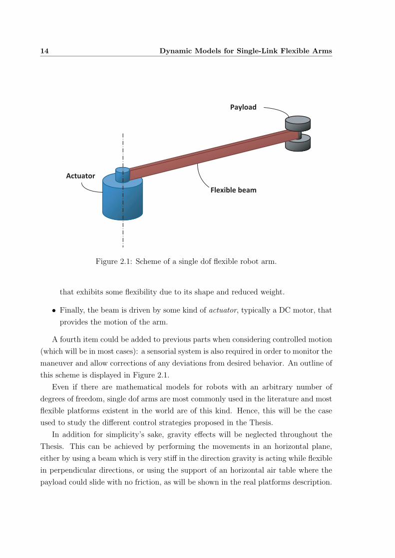
14 Dynamic Models for Single-Link Flexible Arms
Actuator
Flexible beam
Payload
Figure 2.1: Scheme of a single dof flexible robot arm.
that exhibits some flexibility due to its shape and reduced weight.
• Finally, the beam is driven by some kind of actuator, typically a DC motor, that
provides the motion of the arm.
A fourth item could be added to previous parts when considering controlled motion
(which will be in most cases): a sensorial system is also required in order to monitor the
maneuver and allow corrections of any deviations from desired behavior. An outline of
this scheme is displayed in Figure 2.1.
Even if there are mathematical models for robots with an arbitrary number of
degrees of freedom, single dof arms are most commonly used in the literature and most
flexible platforms existent in the world are of this kind. Hence, this will be the case
used to study the different control strategies proposed in the Thesis.
In addition for simplicity’s sake, gravity effects will be neglected throughout the
Thesis. This can be achieved by performing the movements in an horizontal plane,
either by using a beam which is very stiff in the direction gravity is acting while flexible
in perpendicular directions, or using the support of an horizontal air table where the
payload could slide with no friction, as will be shown in the real platforms description.
2.2. Actuator model 15
The physical drawback of using light beams for robotics is very simple: beam
flexibility produces a deflection in the link which causes a misalignment between motor
angle, θm, and tip angle, θt. However, the modeling and control of this kind of robotic
systems is not that easy, and therefore, a number of different mathematical templates
have been used to describe this phenomenon. Some of them have been chosen because
of their simplicity or completeness in idealizing the actual platforms. They will be
presented subsequently.
The model used for the actuator is presented in Section 2.2, as it is common to
all of the platforms described afterwards. Subsequently, some classical approaches for
modeling flexibility in beams are detailed. First, the distributed masses equivalent
model is presented in Section 2.3, jointly with the procedure to obtain the transfer
functions of the system truncated to a finite number of modes of vibration. Next,
Section 2.4 presents a concentrated masses model for describing the beam+payload
system, concentrating on two cases: negligible beam mass and beam mass concentrated
at its middle point. To finish, Section 2.5 introduces a novel model for flexible systems
subject to strong geometric non-linearities which is based on a duffing-like equation
(Thompson and Stewart, 2002) with the addition of variant coefficients.
These models lie beneath the real platforms that are to be detailed next. All used
platforms are listed and detailed in Section 2.6. Namely, an old-generation duralu-
minium arm, which is driven by a DC-motor and allows a payload of up to 5 kg,
and a much lighter and safer new-generation composites arm, also DC-motor driven
that allows movement up to 200g. In the same Section, the sensorial system used to
instrument the platforms is also described.
2.2 Actuator model
As mentioned in previous Section, a mathematical definition for the actuator must
be provided for any complete model of a flexible arm. It is and is common and necessary
for all models.
The actuator chosen to drive the links in all platforms is a DC motor which has a
reduction gear with a reduction relation nr. That increases the strength of the system
while diminishing its velocity. Taking into account that the maximum angular velocity
16 Dynamic Models for Single-Link Flexible Arms
of a DC motor is usually much higher than needed, this gear-box reduces the size of
the selected motor for driving a specific payload while keeping a sufficient maximum
output velocity. It also reduces the effect of the beam-payload coupled inertia in the
motor. Note that the magnitudes seen from the motor side of the gear will be written
with an upper hat, while the magnitudes seen from the link side will be denoted by
standard letters.
The dynamics of the motor with a closed loop current control system (where the
voltage Vm is assumed to be proportional to the current) is given by
Γm = KmVm = Jm¨θm + ν
˙θm + Γcoup + ΓCoul (2.1)
where · denotes differentiation with respect to time, Γm is the torque produced by the
motor, Km is a motor constant, Vm is the voltage signal that controls the motor, Jm
is the motor inertia, ν is the viscous friction coefficient, Γcoup is the coupling torque
between the motor and the link, and ΓCoul is the Coulomb friction. The conversion
equations between magnitudes, valid for any angle or torque involved in the actuator
model equations, are given by
θ = nrθ Γ =Γ
nr
(2.2)
The last term of equation (2.1) is assumed to be negligible or compensated, as
shown in (Feliu et al., 1993), with a compensation term of the form
VCoul =ΓCoul
Km
sign(˙θm
)(2.3)
where ΓCoul is an estimation of the Coulomb friction value. On the other hand, as-
suming that the coupling torque can be measured or estimated from measurements,
another compensation term of the form
Vcoup =Γcoup
Km
=Γcoup
Kmnr
(2.4)
that counteracts the effect of the arm inertia and decouples motor and link dynamics,
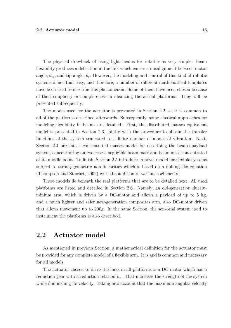
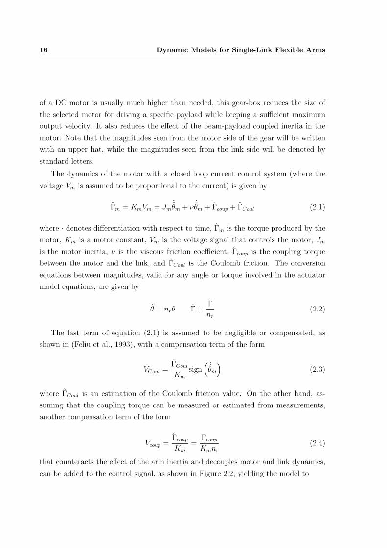
can be added to the control signal, as shown in Figure 2.2, yielding the model to
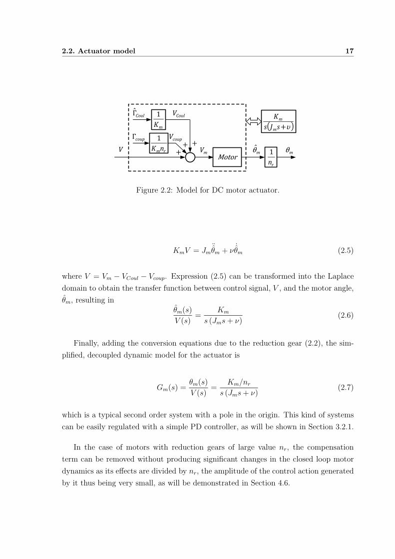
2.2. Actuator model 17
V
coup
Coul !
mV
" #$%sJsK
m
m
m&!
m&%
%%rmnK
'
rn
'
mK
' CoulV
coupV
Figure 2.2: Model for DC motor actuator.
KmV = Jm¨θm + ν
˙θm (2.5)
where V = Vm − VCoul − Vcoup. Expression (2.5) can be transformed into the Laplace
domain to obtain the transfer function between control signal, V , and the motor angle,
θm, resulting inθm(s)
V (s)=
Km
s (Jms+ ν)(2.6)
Finally, adding the conversion equations due to the reduction gear (2.2), the sim-
plified, decoupled dynamic model for the actuator is
Gm(s) =θm(s)
V (s)=
Km/nr
s (Jms+ ν)(2.7)
which is a typical second order system with a pole in the origin. This kind of systems
can be easily regulated with a simple PD controller, as will be shown in Section 3.2.1.
In the case of motors with reduction gears of large value nr, the compensation
term can be removed without producing significant changes in the closed loop motor
dynamics as its effects are divided by nr, the amplitude of the control action generated
by it thus being very small, as will be demonstrated in Section 4.6.
18 Dynamic Models for Single-Link Flexible Arms
2.3 Distributed masses model
These models consider flexible links as a continuum. They are calculated as the
solution of the partial differential equation that characterizes the system which can be
obtained e.g. applying variable separation and modal expansion.
Modal expansion method has been widely used in previous work (Nicosia et al.,
1986; Bellezza et al., 1990; Boyer and Coiffet, 1996) for modeling flexible manipula-
tors. Starting from the Euler-Bernouilli equation, and assuming the link possesses an
infinite number of natural frequencies, we obtain a truncated model with n modes of
vibration. These are usually the lowest frequency modes as they are the most signifi-
cant, (biggest amplitudes), to the system dynamics. Once the modes are known, the
link displacements are presented as the product of two terms, a spacial term (modal
functions, ϕi(x)), and a temporal term (generalized coordinates, qi(t)) as expressed in
following equation:
w(x, t) =∑i
ϕi(x)qi(t) (2.8)
The modal functions must fulfill three conditions:
• They must constitute a complete coordinate base, that is, this set of functions
must be able to express the displacement of any point of the link.
• The functions must satisfy the geometric boundary conditions.
• They must be differentiable over the defined domain, at least up to the degree of
the differential equation that rules the model.
In addition, modal functions fulfill some ortogonality conditions which lead to some
simplifications in the model (Clough and Penzien, 1993). On its part, generalized
coordinates compose a set of time-dependent parameters which are independent among
them.
Once modal functions are calculated, there exist two ways to address the dynamic
modeling of the system: by means of Lagrange Equations (Book, 1984; DeLuca and
Siciliano, 1991) or through Newton-Euler Equations (Rakhsha and Goldenberg, 1986;
Boyer and Coiffet, 1996). In this section, the first method is presented using the
2.3. Distributed masses model 19
example to obtain a model with three modes of vibration. We will assume that the
manipulator consists of a distributed mass link with a point mass attached to its end
and whose movement is restricted to an horizontal plane. In addition, the pseudo-
pinned formulation will be adopted for solving the Euler-Bernouilli equation, that is,
the x-axis of the rotary frame, X−Y, intersects the center of mass of the arm as shown
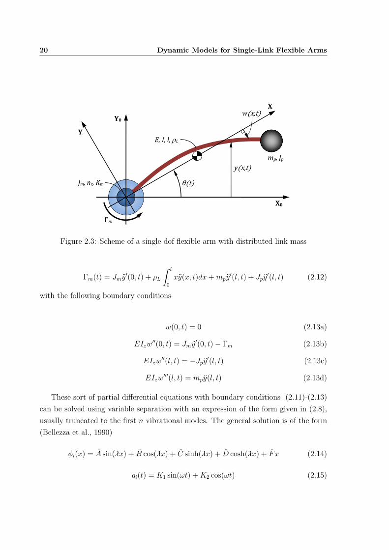
in Figure 2.3 (Bellezza et al., 1990). Following hypotheses are adopted:
• The material of the link is continuous, uniform, homogeneous and isotropic.
• Small transversal displacements.
• Navier hypothesis are assumed to be valid, that is, flat sections remain flat after
deformation.
• Torsional effects are negligible.
Next the dynamic model will be obtained.
2.3.1 Solution of the Euler-Bernouilli Equation
Taking into account the previously adopted hypothesis and the Hamilton’s princi-
ple (Meirovitch, 1997), the behavior of an Euler-Bernouilli beam is governed by the
following fourth order partial differential equation
EIz∂4w(x, t)
∂x4+ ρL
∂2w(x, t)
∂t2= fd(x, t) (2.9)
where w(x, t) is the deflection at point x of the beam, and fd(x, t) is the external
distributed force.
Defining the position of a point x of the link with respect to the fixed frame as
y(t, x) = θ(t)x+ w(x, t) (2.10)
and applying expression (2.9) to the case of a flexible arm under the effect of an
input torque, Γm, due to motor action, the following boundary value problem can be
formulated
EIzwiv(x, t) + ρLy(x, t) = 0 (2.11)
20 Dynamic Models for Single-Link Flexible Arms
Y0
X0
!"
E, I, l, !L
#$%
Jm, nr, Km
mp, Jp
Y
X
w &'!"
y &'!"
Figure 2.3: Scheme of a single dof flexible arm with distributed link mass
Γm(t) = Jmy′(0, t) + ρL
∫ l
0
xy(x, t)dx+mpy′(l, t) + Jpy
′(l, t) (2.12)
with the following boundary conditions
w(0, t) = 0 (2.13a)
EIzw′′(0, t) = Jmy
′(0, t)− Γm (2.13b)
EIzw′′(l, t) = −Jpy
′(l, t) (2.13c)
EIzw′′′(l, t) = mpy(l, t) (2.13d)
These sort of partial differential equations with boundary conditions (2.11)-(2.13)
can be solved using variable separation with an expression of the form given in (2.8),
usually truncated to the first n vibrational modes. The general solution is of the form
(Bellezza et al., 1990)
ϕi(x) = A sin(λx) + B cos(λx) + C sinh(λx) + D cosh(λx) + F x (2.14)
qi(t) = K1 sin(ωt) +K2 cos(ωt) (2.15)

2.3. Distributed masses model 21
being λ4 = ω2mEIz
. The values of K1 and K2 depend on the initial conditions of position
and velocity: K1 = q(0)/ω and K2 = q(0). On the other hand, A, B, C, D and F are
obtained from the boundary conditions of Eq. (2.14). They are
y(t, 0) = 0 (2.16a)
EIzy′′(t, 0) + Γm − Jmθ = 0 (2.16b)
EIzy′′(t, l) + Jey
′(t, l) = 0 (2.16c)
EIzy′′′(t, l)−my(t, l) = 0. (2.16d)
2.3.2 System model in space-state form
Rearranging previous expressions (Feliu, 1997), the solution to the Euler-Bernouilli
equation in a space-state form is
Xs = AXs +BΓm
Ys = CXs +DΓm
(2.17)
where the state variables are the generalized coordinates qi and the matrix dimensions
depend on the number of vibration modes considered. Taking n modes into account,
the state vector is Xs = [q0 . . . qn q0 . . . qn]T , T denoting matrix transpose, and the
space-state matrixes are
A =
[0(n+1)×(n+1) In+1
Ω(n+1)×(n+1) 0(n+1)×(n+1)
]B =
1
J
0(n+1)×1
1
ϕ′1(0)...
ϕ′n(0)
(2.18)
where 0p×n is a matrix of p rows and n columns of zeros, In is the identity matrix of
dimension n, and Ω(n+1)×(n+1) is a matrix defined as follows
22 Dynamic Models for Single-Link Flexible Arms
Ω(n+1)×(n+1) =
0 0 · · · 0
0 ω21 · · · 0
......
. . ....
0 0 · · · ω2n
(2.19)
Matrixes C and D depend on the desired output. Specifically, we will consider the
motor angular position, the payload angular position and the coupling torque of the
system, that is Ys = [θm θt Γcoup]T . To calculate this outputs, the values for C and D
are
C =
1 ϕ′1(0) · · · ϕ′
n(0) 0 · · · 0
1 ϕ′1(l) · · · ϕ′
n(l) 0 · · · 0
0 −EIϕ′′1(l) · · · −EIϕ′′
n(l) 0 · · · 0
D =
000
(2.20)
The dimensions of the matrixes are A ∈ ℜ(2n+2)×(2n+2), B ∈ ℜ(2n+2)×1, C ∈ℜp×(2n+2) and D ∈ ℜp×1, the state vector is Xs ∈ ℜ(2n+2)×1 and outputs vector is
Ys ∈ ℜp×1.
2.4 Concentrated masses model
In this case, the system we want to model consists of a flexible link whose mass
is assumed to be concentrated in a certain number of points along itself (Feliu et al.,
1991). The number of vibration modes in the structure match the number of point
masses along the beam. Advantages of this method are
• Dynamics are simpler to model in comparison with distributed mass arms.
• Payload changes are straightaway applied to the model.
• Since the distributed mass model of a flexible link is usually truncated to a finite
number of vibration modes, we can find a concentrated masses model with similar
characteristics.
These models are useful when the beam mass is not very significant but cannot be
neglected.
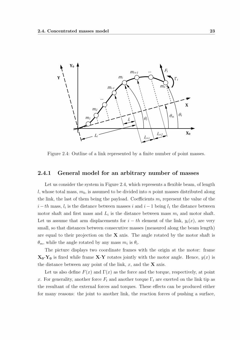
2.4. Concentrated masses model 23
m1
,-
./
.
Y
X
Y0
X0
0$
, 1
$
21/
31
31)!31)4
$
,15!/
,1
,1)!
m2
Figure 2.4: Outline of a link represented by a finite number of point masses.
2.4.1 General model for an arbitrary number of masses
Let us consider the system in Figure 2.4, which represents a flexible beam, of length
l, whose total mass, mb, is assumed to be divided into n point masses distributed along
the link, the last of them being the payload. Coefficients mi represent the value of the
i− th mass, li is the distance between masses i and i− 1 being l1 the distance between
motor shaft and first mass and Li is the distance between mass mi and motor shaft.
Let us assume that arm displacements for i − th element of the link, yi(x), are very
small, so that distances between consecutive masses (measured along the beam length)
are equal to their projection on the X axis. The angle rotated by the motor shaft is
θm, while the angle rotated by any mass mi is θi.
The picture displays two coordinate frames with the origin at the motor: frame
X0-Y0 is fixed while frame X-Y rotates jointly with the motor angle. Hence, y(x) is
the distance between any point of the link, x, and the X axis.
Let us also define F (x) and Γ(x) as the force and the torque, respectively, at point
x. For generality, another force Ft and another torque Γt are exerted on the link tip as
the resultant of the external forces and torques. These effects can be produced either
for many reasons: the joint to another link, the reaction forces of pushing a surface,
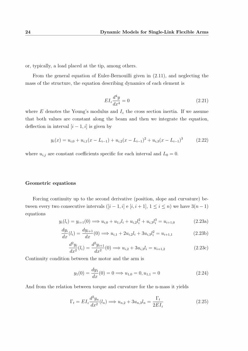
24 Dynamic Models for Single-Link Flexible Arms
or, typically, a load placed at the tip, among others.
From the general equation of Euler-Bernouilli given in (2.11), and neglecting the
mass of the structure, the equation describing dynamics of each element is
EIzd4y
dx4= 0 (2.21)
where E denotes the Young’s modulus and Iz the cross section inertia. If we assume
that both values are constant along the beam and then we integrate the equation,
deflection in interval [i− 1, i] is given by
yi(x) = ui,0 + ui,1(x− Li−1) + ui,2(x− Li−1)2 + ui,3(x− Li−1)
3 (2.22)
where ui,j are constant coefficients specific for each interval and L0 = 0.
Geometric equations
Forcing continuity up to the second derivative (position, slope and curvature) be-
tween every two consecutive intervals ([i− 1, i] e [i, i+ 1], 1 ≤ i ≤ n) we have 3(n− 1)
equations
yi(li) = yi+1(0) =⇒ ui,0 + u1,ili + ui,2l2i + ui,3l
3i = ui+1,0 (2.23a)
dyidx
(li) =dyi+1
dx(0) =⇒ ui,1 + 2ui,2li + 3ui,3l
2i = ui+1,1 (2.23b)
d2yidx2
(li) =d2yi+1
dx2(0) =⇒ ui,2 + 3ui,3li = ui+1,2 (2.23c)
Continuity condition between the motor and the arm is
y1(0) =dy1dx
(0) = 0 =⇒ u1,0 = 0, u1,1 = 0 (2.24)
And from the relation between torque and curvature for the n-mass it yields
Γt = EIzd2yndx2
(ln) =⇒ un,2 + 3un,3ln =Γt
2EIz(2.25)
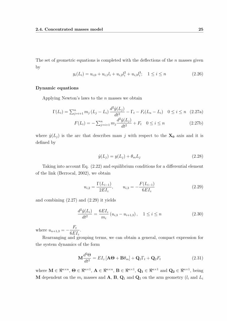
2.4. Concentrated masses model 25
The set of geometric equations is completed with the deflections of the n masses given
by
yi(Li) = ui,0 + ui,1li + ui,2l2i + ui,3l
3i ; 1 ≤ i ≤ n (2.26)
Dynamic equations
Applying Newton’s laws to the n masses we obtain
Γ(Li) =∑n
j=i+1 mj (Lj − Li)d2y(Lj)
dt2− Γt − Ft(Ln − Li) 0 ≤ i ≤ n (2.27a)
F (Li) = −∑n
j=i+1 mjd2y(Lj)
dt2+ Ft 0 ≤ i ≤ n (2.27b)
where y(Lj) is the arc that describes mass j with respect to the X0 axis and it is
defined by
y(Lj) = y(Lj) + θmLj (2.28)
Taking into account Eq. (2.22) and equilibrium conditions for a differential element
of the link (Berrocal, 2002), we obtain
ui,2 =Γ(Li−1)
2EIz, ui,3 = −F (Li−1)
6EIz(2.29)
and combining (2.27) and (2.29) it yields
d2y(Li)
dt2=
6EIzmi
(ui,3 − ui+1,3) , 1 ≤ i ≤ n (2.30)
where un+1,3 = − Ft
6EIz.
Rearranging and grouping terms, we can obtain a general, compact expression for
the system dynamics of the form
Md2Θ
dt2= EIz [AΘ+Bθm] +Q1Γt +Q2Ft (2.31)
where M ∈ ℜn×n, Θ ∈ ℜn×1, A ∈ ℜn×n, B ∈ ℜn×1, Q1 ∈ ℜn×1 and Q2 ∈ ℜn×1, being
M dependent on the mi masses and A, B, Q1 and Q2 on the arm geometry (li and Li
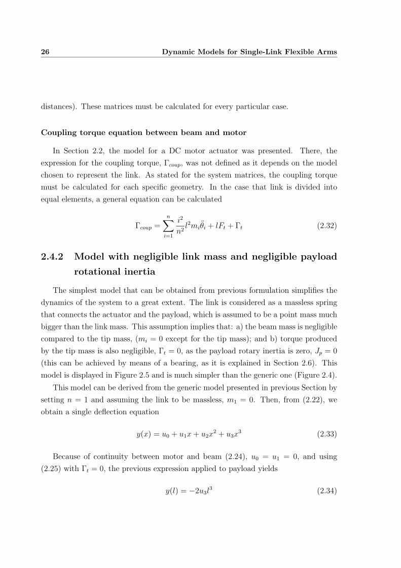
26 Dynamic Models for Single-Link Flexible Arms
distances). These matrices must be calculated for every particular case.
Coupling torque equation between beam and motor
In Section 2.2, the model for a DC motor actuator was presented. There, the
expression for the coupling torque, Γcoup, was not defined as it depends on the model
chosen to represent the link. As stated for the system matrices, the coupling torque
must be calculated for each specific geometry. In the case that link is divided into
equal elements, a general equation can be calculated
Γcoup =n∑
i=1
i2
n2l2miθi + lFt + Γt (2.32)
2.4.2 Model with negligible link mass and negligible payload
rotational inertia
The simplest model that can be obtained from previous formulation simplifies the
dynamics of the system to a great extent. The link is considered as a massless spring
that connects the actuator and the payload, which is assumed to be a point mass much
bigger than the link mass. This assumption implies that: a) the beam mass is negligible
compared to the tip mass, (mi = 0 except for the tip mass); and b) torque produced
by the tip mass is also negligible, Γt = 0, as the payload rotary inertia is zero, Jp = 0
(this can be achieved by means of a bearing, as it is explained in Section 2.6). This
model is displayed in Figure 2.5 and is much simpler than the generic one (Figure 2.4).
This model can be derived from the generic model presented in previous Section by
setting n = 1 and assuming the link to be massless, m1 = 0. Then, from (2.22), we
obtain a single deflection equation
y(x) = u0 + u1x+ u2x2 + u3x
3 (2.33)
Because of continuity between motor and beam (2.24), u0 = u1 = 0, and using
(2.25) with Γt = 0, the previous expression applied to payload yields
y(l) = −2u3l3 (2.34)
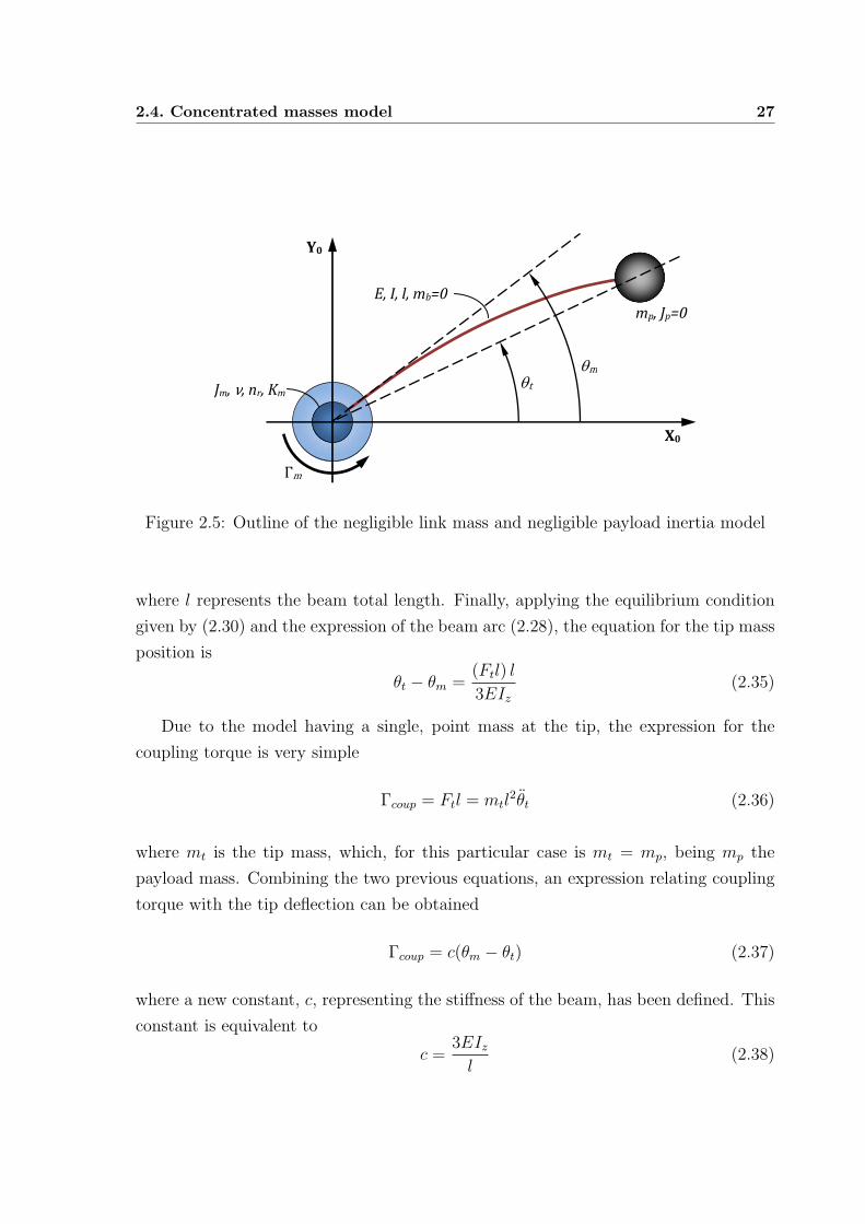
2.4. Concentrated masses model 27
Y0
X0
!
E, I, l, mb=0
" #
Jm, $, nr, Km
mp, Jp=0
!
J $
&
Figure 2.5: Outline of the negligible link mass and negligible payload inertia model
where l represents the beam total length. Finally, applying the equilibrium condition
given by (2.30) and the expression of the beam arc (2.28), the equation for the tip mass
position is
θt − θm =(Ftl) l
3EIz(2.35)
Due to the model having a single, point mass at the tip, the expression for the
coupling torque is very simple
Γcoup = Ftl = mtl2θt (2.36)
where mt is the tip mass, which, for this particular case is mt = mp, being mp the
payload mass. Combining the two previous equations, an expression relating coupling
torque with the tip deflection can be obtained
Γcoup = c(θm − θt) (2.37)
where a new constant, c, representing the stiffness of the beam, has been defined. This
constant is equivalent to
c =3EIzl
(2.38)
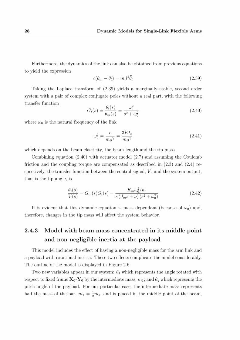
28 Dynamic Models for Single-Link Flexible Arms
Furthermore, the dynamics of the link can also be obtained from previous equations
to yield the expression
c(θm − θt) = mtl2θt (2.39)
Taking the Laplace transform of (2.39) yields a marginally stable, second order
system with a pair of complex conjugate poles without a real part, with the following
transfer function
Gt(s) =θt(s)
θm(s)=
ω20
s2 + ω20
(2.40)
where ω0 is the natural frequency of the link
ω20 =
c
mtl2=
3EIzmtl3
(2.41)
which depends on the beam elasticity, the beam length and the tip mass.
Combining equation (2.40) with actuator model (2.7) and assuming the Coulomb
friction and the coupling torque are compensated as described in (2.3) and (2.4) re-
spectively, the transfer function between the control signal, V , and the system output,
that is the tip angle, is
θt(s)
V (s)= Gm(s)Gt(s) =
Kmω20/nr
s (Jms+ ν) (s2 + ω20)
(2.42)
It is evident that this dynamic equation is mass dependant (because of ω0) and,
therefore, changes in the tip mass will affect the system behavior.
2.4.3 Model with beam mass concentrated in its middle point
and non-negligible inertia at the payload
This model includes the effect of having a non-negligible mass for the arm link and
a payload with rotational inertia. These two effects complicate the model considerably.
The outline of the model is displayed in Figure 2.6.
Two new variables appear in our system: θ1 which represents the angle rotated with
respect to fixed frameX0-Y0 by the intermediate mass, m1; and θg which represents the
pitch angle of the payload. For our particular case, the intermediate mass represents
half the mass of the bar, m1 = 12mb, and is placed in the middle point of the beam,
2.4. Concentrated masses model 29
Y0
X0
!
E, I, l
" #
Jm, $, nr, Km
mp, Jp
%#
&
m1
Figure 2.6: Outline of the model taking into account link mass and payload inertia
splitting the link into two equal length pieces with l1 = l2 = 12l. On the other hand,
the tip mass is determined by mt = mp +14mb. Again applying the generic equation of
a beam for each of the links, we obtain two expressions
y1(x) = u1,0 + u1,1x+ u1,2x2 + u1,3x
3 ∀x ∈ [0, l/2] (2.43a)
y2(x) = u2,0 + u2,1x+ u2,2x2 + u2,3x
3 ∀x ∈ [l/2, l] (2.43b)
Eight equations are necessary to determine ui,j constants. Five of them are obtained
from continuity conditions stated in (2.23). Applied to this particular case:
y1(0) = y′1(0) = 0 (2.44a)
y1(l/2) = y2(l/2) (2.44b)
y′1(l/2) = y′2(l/2) (2.44c)
y′′1(l/2) = y′′2(l/2) (2.44d)
where ′ represents the derivative with respect to x. The remaining equations are
obtained from dynamic conditions (2.30), yielding
30 Dynamic Models for Single-Link Flexible Arms
EIzy′′2(l) = −Jpθg (2.45a)
EIzy′′1(l/2) = −Jpθg +
1
2mtl
2θt (2.45b)
EIzy′′1(0) = −Jpθg +mtl
2θt −1
4m1l
2θ1 (2.45c)
Combining expressions (2.43), (2.44) and (2.45) and rearranging terms, so that the
input to the system is the motor angle, θm, and the outputs are the angles of the
masses, θ1 and θt and the payload pitch θg, the dynamic state equations of the system
can be obtained,
Xs =
A︷ ︸︸ ︷03×3 I3
−192δ 192δ −48δ
48ρ −60ρ 18ρ 03×3
−12δ 18δ −7δ
Xs +
B︷ ︸︸ ︷03×1
48δ
−6ρ
γ
θm
Ys =[I3×3 03×3
]︸ ︷︷ ︸
C
Xs + [03×1]︸ ︷︷ ︸D
θm
(2.46)
where the vector of states is X =[θ1 θt θg θ1 θt θg
]Tand the following con-
stants
γ =EI
Jpl, ρ =
EI
mtl3δ =
EI
m1l3(2.47)
have been defined for the sake of concision. From (2.46) it is quite straightforward to
obtain the transfer functions between the outputs and the input of the system, resulting
in
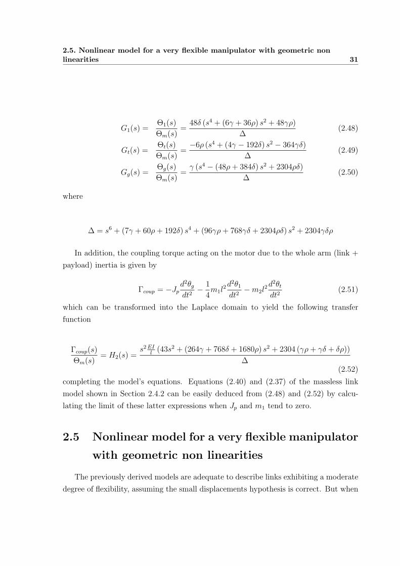
2.5. Nonlinear model for a very flexible manipulator with geometric nonlinearities 31
G1(s) =Θ1(s)
Θm(s)=
48δ (s4 + (6γ + 36ρ) s2 + 48γρ)
∆(2.48)
Gt(s) =Θt(s)
Θm(s)=
−6ρ (s4 + (4γ − 192δ) s2 − 364γδ)
∆(2.49)
Gg(s) =Θg(s)
Θm(s)=
γ (s4 − (48ρ+ 384δ) s2 + 2304ρδ)
∆(2.50)
where
∆ = s6 + (7γ + 60ρ+ 192δ) s4 + (96γρ+ 768γδ + 2304ρδ) s2 + 2304γδρ
In addition, the coupling torque acting on the motor due to the whole arm (link +
payload) inertia is given by
Γcoup = −Jpd2θgdt2
− 1
4m1l
2d2θ1dt2
−m2l2d
2θtdt2
(2.51)
which can be transformed into the Laplace domain to yield the following transfer
function
Γcoup(s)
Θm(s)= H2(s) =
s2EIl(43s2 + (264γ + 768δ + 1680ρ) s2 + 2304 (γρ+ γδ + δρ))
∆(2.52)
completing the model’s equations. Equations (2.40) and (2.37) of the massless link
model shown in Section 2.4.2 can be easily deduced from (2.48) and (2.52) by calcu-
lating the limit of these latter expressions when Jp and m1 tend to zero.
2.5 Nonlinear model for a very flexible manipulator
with geometric non linearities
The previously derived models are adequate to describe links exhibiting a moderate
degree of flexibility, assuming the small displacements hypothesis is correct. But when
32 Dynamic Models for Single-Link Flexible Arms
the link presents large tip displacements, some of assumptions adopted in the resolution
of the Euler-Bernouilli Equation are no longer valid.
In previous literature, some work has also been devoted to model large elastic dis-
placements. Based on the Euler-Bernouilli equation, numerical algorithms have been
proposed to estimate the curvature and tip deflection of a static elastic beam. These
methods rely on the solution of complicated integral equations by numerical meth-
ods (Wang, 1981; Belendez et al., 2002), numerical solution of nonlinear differential
equations ((Lee, 2002) for fixed cross sections and nonlinear elastic materials and (Lee
et al., 1993) for variable cross section), or the use of sensors (strain gauges) that mea-
sure the curvatures at certain points of the beam followed by a polynomial interpolation
(Gu and Piedboeuf, 2003).
Some of the modeling techniques mentioned above give precise descriptions of the
geometrical nonlinear dynamics of the flexible beam. These models are based on nu-
merical approximations of differential or integral equations that have to be solved at
every considered time, or they are represented by means of complicated analytical dif-
ferential equations. They are well suited for numerical simulations or for calculating
command profiles (usually motor torques) to be applied in an open loop fashion to the
arm in order to follow a desired tip trajectory. But these models can hardly be applied
to analyze and design nonlinear closed loop control systems for these arms. At most,
linearized models of local validity around the desired trajectory can be derived from
the previous models, which may lead to local linear controllers that need to be updated
in real time in response to the state of the arm.
However, we are interested in simple nonlinear dynamic models, that capture the
most important dynamics of the arm while remaining useful for the design of arm tip
position nonlinear controllers. That is, the desired nonlinear model should still remain
computationally light, allowing it to be applied to real platforms.
For these reasons, a new model with these features is presented (Payo et al., 2005).
A general model is attained from the Euler-Bernouilli beam equation and then the
equations are particularized for a concentrated masses model with a single point mass
at the tip which is subject to a force. These equations are applied to the linear sys-
tem, obtaining an equivalent expression to that of Section 2.4.2, and to the non-linear
system, which yields a non-linear expression computationally light and much more rep-
2.5. Nonlinear model for a very flexible manipulator with geometric nonlinearities 33
resentative of the actual behavior of the real platform, as is demonstrated latter by
means of latter experimentation.
2.5.1 On the Euler-Bernouilli beam
A flexible beam exhibits a nonlinear behavior when it is under the effects of large
forces (Landau and Lifshitz, 1969). Assuming that our composite material remains
linearly elastic and there is not a change of status, this nonlinear behavior is due to
a change in the geometric layout of the bar (geometric nonlinearities) due to bending
and/or torsional moments. Under the assumption that torsional effects are negligible,
the equation of Euler-Bernoulli for large deflections is
dθpds
=d2y′
dx′2
(1 + ( dy′
dx′ )2)32
=Mz
EIz(2.53)
where θp is the orientation of the beam at point p ′, and s is the arc length over the
beam, x′ and y′ are the coordinates of a point of the beam expressed in a cartesian
frame, X−Y, according to Figure 2.7, Mz is the bending moment on any section of
the beam and EIz is the stiffness of the bar. For small deflections s is equal to x′,
and the rotation angle θp can be approximated by dy′/dx′ yielding that dθp/ds can be
approximated by d2y′/dx′2. Then, equation of Euler-Bernoulli (2.9) simplifies to the
well-known small displacements equation used for previous models (2.21).
However, for large deflections these simplifications are not valid and it is necessary
to use the above equation (2.53) in its complete form. The solution of this equation
can be obtained by calculating some elliptic integrals, which can be evaluated using
numerical methods (Wang, 1981; Belendez et al., 2002). Equation (2.53) does not have
an analytical solution.
Let us consider Figure 2.7, where a force F is applied at the tip of the beam. This
force produces a torque along the beam which is equal to the bending moment Mz. Let
us denote the magnitude of this force as F and its orientation as φ. Then, the static
(kinematic) equation of the beam is obtained from (Landau and Lifshitz, 1969)
d2θpds2
=F
EIzsin(θp − φ) 0 ≤ s ≤ l (2.54)
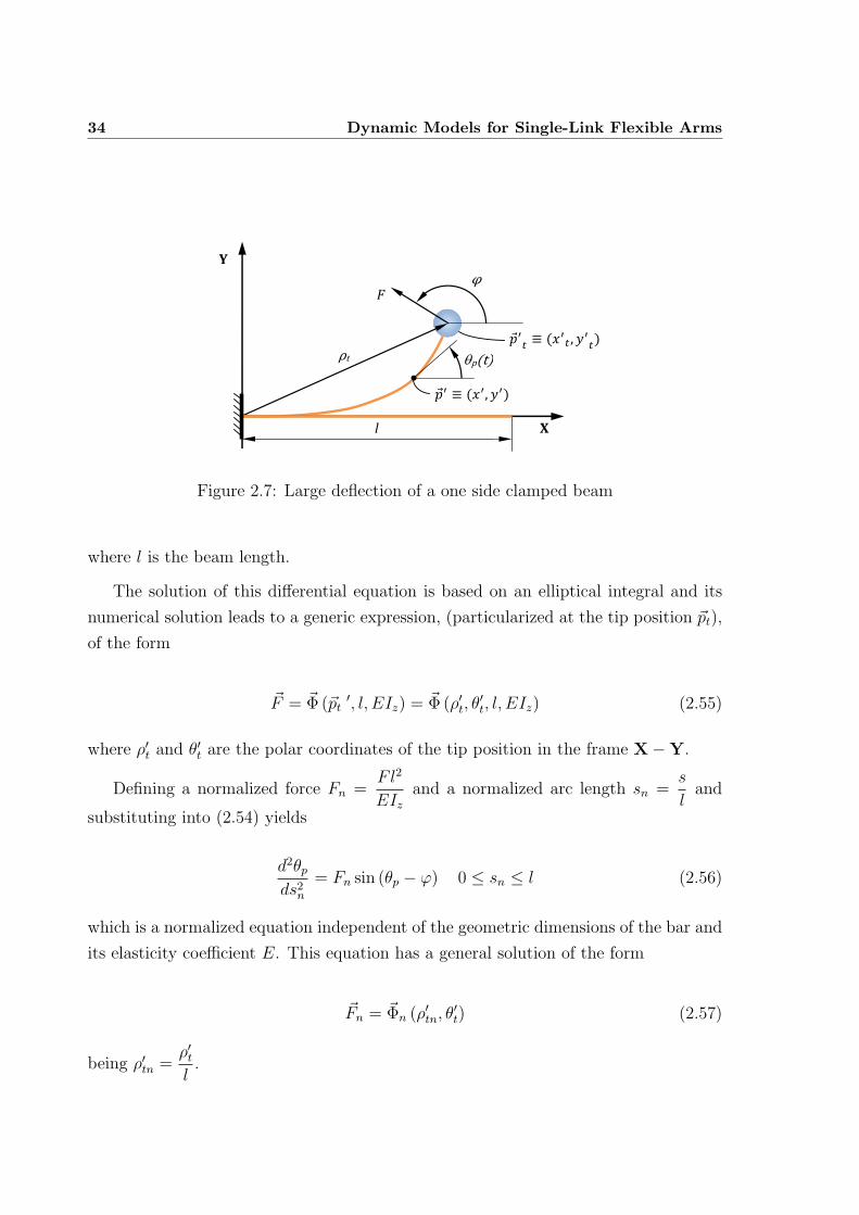
34 Dynamic Models for Single-Link Flexible Arms
Y
X
!"#
$%& ' !(&) *&#
F
+
,"
l
$%&-' !(&- ) *
&-#
Figure 2.7: Large deflection of a one side clamped beam
where l is the beam length.
The solution of this differential equation is based on an elliptical integral and its
numerical solution leads to a generic expression, (particularized at the tip position pt),
of the form
F = Φ (pt′, l, EIz) = Φ (ρ′t, θ
′t, l, EIz) (2.55)
where ρ′t and θ′t are the polar coordinates of the tip position in the frame X−Y.
Defining a normalized force Fn =Fl2
EIzand a normalized arc length sn =
s
land
substituting into (2.54) yields
d2θpds2n
= Fn sin (θp − φ) 0 ≤ sn ≤ l (2.56)
which is a normalized equation independent of the geometric dimensions of the bar and
its elasticity coefficient E. This equation has a general solution of the form
Fn = Φn (ρ′tn, θ
′t) (2.57)
being ρ′tn =ρ′tl.
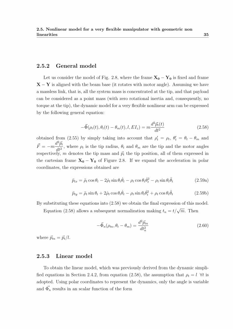
2.5. Nonlinear model for a very flexible manipulator with geometric nonlinearities 35
2.5.2 General model
Let us consider the model of Fig. 2.8, where the frame X0 −Y0 is fixed and frame
X−Y is aligned with the beam base (it rotates with motor angle). Assuming we have
a massless link, that is, all the system mass is concentrated at the tip, and that payload
can be considered as a point mass (with zero rotational inertia and, consequently, no
torque at the tip), the dynamic model for a very flexible nonlinear arm can be expressed
by the following general equation:
−Φ(ρt(t), θt(t)− θm(t), l, EIz) = md2pt(t)
dt2(2.58)
obtained from (2.55) by simply taking into account that ρ′t = ρt, θ′t = θt − θm and
F = −md2ptdt2
, where ρt is the tip radius, θt and θm are the tip and the motor angles
respectively, m denotes the tip mass and pt the tip position, all of them expressed in
the cartesian frame X0 −Y0 of Figure 2.8. If we expand the acceleration in polar
coordinates, the expressions obtained are
ptx = ρt cos θt − 2ρt sin θtθt − ρt cos θtθ2t − ρt sin θtθt (2.59a)
pty = ρt sin θt + 2ρt cos θtθt − ρt sin θtθ2t + ρt cos θtθt (2.59b)
By substituting these equations into (2.58) we obtain the final expression of this model.
Equation (2.58) allows a subsequent normalization making tn = t/√m. Then
−Φn(ρtn, θt − θm) =d2ptndt2n
(2.60)
where ptn = pt/l.
2.5.3 Linear model
To obtain the linear model, which was previously derived from the dynamic simpli-
fied equations in Section 2.4.2, from equation (2.58), the assumption that ρt = l ∀t isadopted. Using polar coordinates to represent the dynamics, only the angle is variable
and Φn results in an scalar function of the form
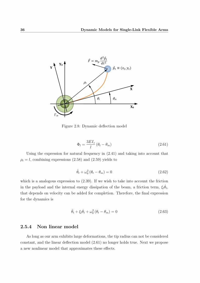
36 Dynamic Models for Single-Link Flexible Arms
Y
X
! " #$
%&'!(%)&
*+
'!( , -.( / 0(1Y0
X0
232+
435
Figure 2.8: Dynamic deflection model
Φl =3EIzl
(θt − θm) (2.61)
Using the expression for natural frequency in (2.41) and taking into account that
ρt = l, combining expressions (2.58) and (2.59) yields to
θt + ω20 (θt − θm) = 0 (2.62)
which is a analogous expression to (2.39). If we wish to take into account the friction
in the payload and the internal energy dissipation of the beam, a friction term, ξlθt,
that depends on velocity can be added for completion. Therefore, the final expression
for the dynamics is
θt + ξlθt + ω20 (θt − θm) = 0 (2.63)
2.5.4 Non linear model
As long as our arm exhibits large deformations, the tip radius can not be considered
constant, and the linear deflection model (2.61) no longer holds true. Next we propose
a new nonlinear model that approximates these effects.
2.5. Nonlinear model for a very flexible manipulator with geometric nonlinearities 37
Nonlinear model for the tip angle
We assume here the equation typically used to model the stiffness of nonlinear
springs
Φnl = αθ′t + βθ′3t (2.64)
In this case, the resulting dynamic equation of the beam is
θt + ξnlθt + α (θt − θm) + β (θt − θm)3 = 0 (2.65)
where α = α/ml2 and β = β/ml2, and again the term ξnlθt incorporates friction into
the model.
Nonlinear model for tip radius
From the equations of the general model, no analytical model for addressing ade-
quately this nonlinearity can be obtained and hence an ad-hoc model had to be adjusted
to represent the phenomena. Extensive numerical simulations of (2.56) for a large range
of values of F have been performed, demonstrating that a good approximation of the
tip radius variation is given by the function
ρt = l cos (γ (θt − θm)) (2.66)
where γ is a constant to be adjusted.
This model implies that changes in ρt basically depend on the component of the
force F which is tangential to the arc motion, being of second order the effects of the
radial component of F .
Complete nonlinear model
Joining both nonlinearities, the final expression for the nonlinear differential equa-
tion governing the system is
θt + ξnlθt +α
cos2 (γ (θt − θm))(θt − θm) +
β
cos2 (γ (θt − θm))(θt − θm)
3 = 0 (2.67)
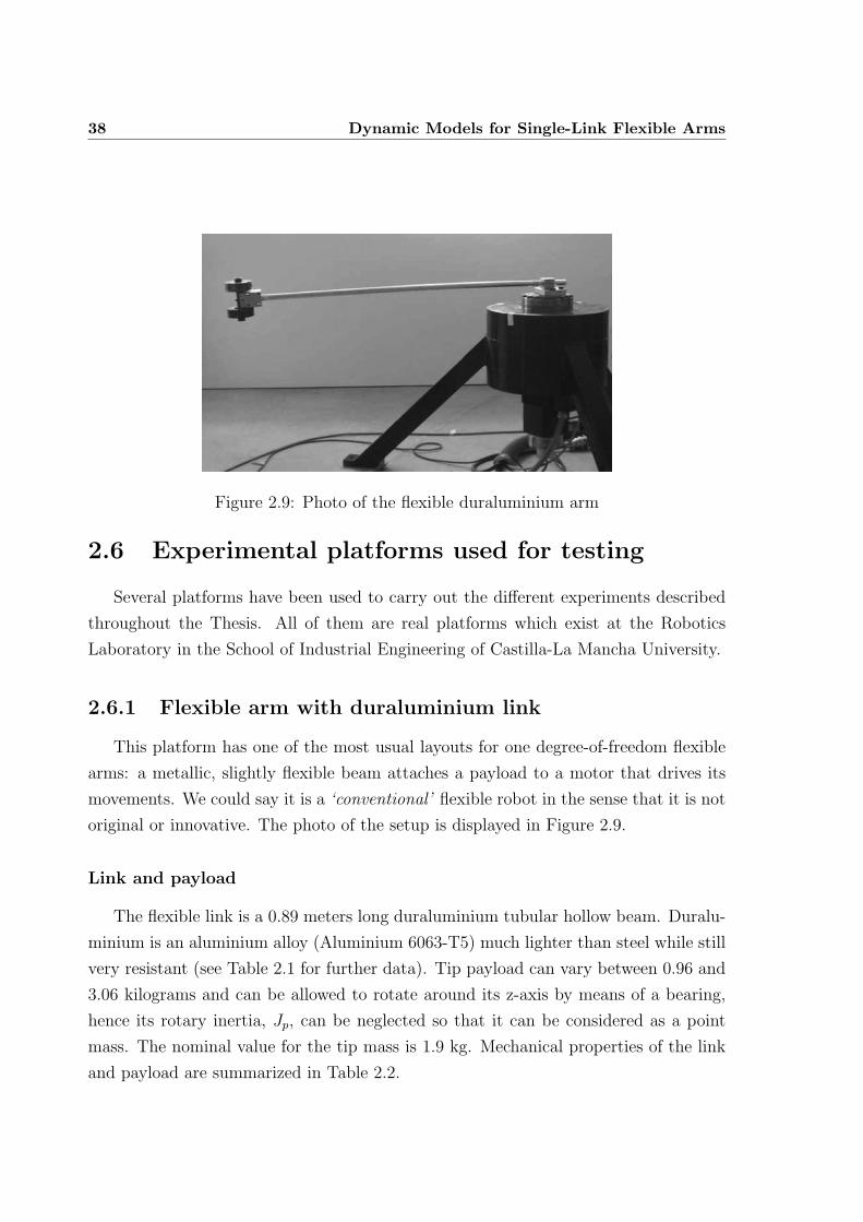
38 Dynamic Models for Single-Link Flexible Arms
Figure 2.9: Photo of the flexible duraluminium arm
2.6 Experimental platforms used for testing
Several platforms have been used to carry out the different experiments described
throughout the Thesis. All of them are real platforms which exist at the Robotics
Laboratory in the School of Industrial Engineering of Castilla-La Mancha University.
2.6.1 Flexible arm with duraluminium link
This platform has one of the most usual layouts for one degree-of-freedom flexible
arms: a metallic, slightly flexible beam attaches a payload to a motor that drives its
movements. We could say it is a ‘conventional’ flexible robot in the sense that it is not
original or innovative. The photo of the setup is displayed in Figure 2.9.
Link and payload
The flexible link is a 0.89 meters long duraluminium tubular hollow beam. Duralu-
minium is an aluminium alloy (Aluminium 6063-T5) much lighter than steel while still
very resistant (see Table 2.1 for further data). Tip payload can vary between 0.96 and
3.06 kilograms and can be allowed to rotate around its z-axis by means of a bearing,
hence its rotary inertia, Jp, can be neglected so that it can be considered as a point
mass. The nominal value for the tip mass is 1.9 kg. Mechanical properties of the link
and payload are summarized in Table 2.2.
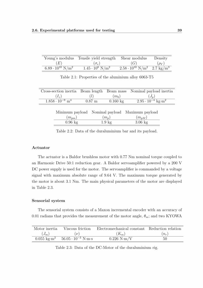
2.6. Experimental platforms used for testing 39
Young’s modulus Tensile yield strength Shear modulus Density(E) (σe) (G) (ρV )
6.89 · 1010 N/m2 1.45 · 108 N/m2 2.58 · 1010 N/m2 2.7 kg/m3
Table 2.1: Properties of the aluminium alloy 6063-T5
Cross-section inertia Beam length Beam mass Nominal payload inertia(Iz) (l) (mb) (Jp)
1.858 · 10−9 m4 0.87 m 0.160 kg 2.95 · 10−4 kg·m2
Minimum payload Nominal payload Maximum payload(mpm) (mp) (mpM)0.96 kg 1.9 kg 3.06 kg
Table 2.2: Data of the duraluminium bar and its payload.
Actuator
The actuator is a Baldor brushless motor with 0.77 Nm nominal torque coupled to
an Harmonic Drive 50:1 reduction gear. A Baldor servoamplifier powered by a 200 V
DC power supply is used for the motor. The servoamplifier is commanded by a voltage
signal with maximum absolute range of 9.64 V. The maximum torque generated by
the motor is about 3.1 Nm. The main physical parameters of the motor are displayed
in Table 2.3.
Sensorial system
The sensorial system consists of a Maxon incremental encoder with an accuracy of
0.01 radians that provides the measurement of the motor angle, θm; and two KYOWA
Motor inertia Viscous friction Electromechanical constant Reduction relation(Jm) (ν) (Km) (nr)
0.055 kg·m2 56.05 · 10−3 N·m·s 0.226 N·m/V 50
Table 2.3: Data of the DC-Motor of the duraluminium rig.
40 Dynamic Models for Single-Link Flexible Arms
strain gauges, arranged in a half-bridge configuration, that measures the motor-beam
coupling torque, Γcoup. This measurement is used to estimate the tip position by
rearranging (2.37) as
θte(t) = θm(t)− Γcoup(t)/c (2.68)
Computer and software
The computer used for control is a Dell Desktop with a Pentium IV processor and
2GB of RAM memory. The Data Acquisition Boards are PCI-NI and the software used
in the control implementation is LabviewTM
7.1.
2.6.2 Flexible arm with composites link
This experimental platform is clearly innovative with respect to the duraluminium
one. The idea is quite the same: a DC-motor drives a flexible link which is attached to
a payload at the far end. However, depending on the length of the link and its material,
the flexibility might be high enough to exhibit geometric nonlinear behavior, which,
for this kind of arms, occurs when there is 0.2 radians difference between the motor
and the tip angles (Belendez et al., 2002). That is, they fall into the categories of one
of the remaining open problems in flexible robotics, which up to now (Benosman and
LeVey, 2004), has not been solved: position control of a geometric nonlinear flexible
arm.
In present Thesis, two different setups have been used in experimentation using
a composites link. The benefits of using composites instead of metallic materials in
robotics are numerous. To mention only some of them:
• Low weight.
• Higher resistance to changes in temperature.
• Higher achievable deflection without permanent deformation.
A more detailed discussion regarding the use of composites in flexible robotics can
be found in (Payo, 2008).
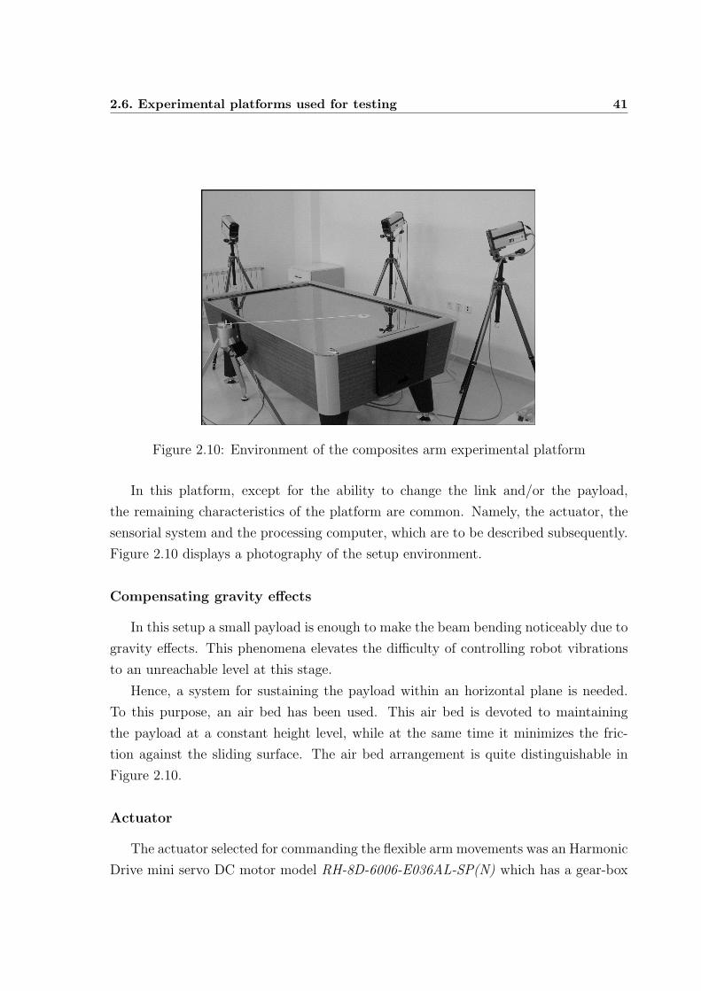
2.6. Experimental platforms used for testing 41
Figure 2.10: Environment of the composites arm experimental platform
In this platform, except for the ability to change the link and/or the payload,
the remaining characteristics of the platform are common. Namely, the actuator, the
sensorial system and the processing computer, which are to be described subsequently.
Figure 2.10 displays a photography of the setup environment.
Compensating gravity effects
In this setup a small payload is enough to make the beam bending noticeably due to
gravity effects. This phenomena elevates the difficulty of controlling robot vibrations
to an unreachable level at this stage.
Hence, a system for sustaining the payload within an horizontal plane is needed.
To this purpose, an air bed has been used. This air bed is devoted to maintaining
the payload at a constant height level, while at the same time it minimizes the fric-
tion against the sliding surface. The air bed arrangement is quite distinguishable in
Figure 2.10.
Actuator
The actuator selected for commanding the flexible arm movements was an Harmonic
Drive mini servo DC motor model RH-8D-6006-E036AL-SP(N) which has a gear-box
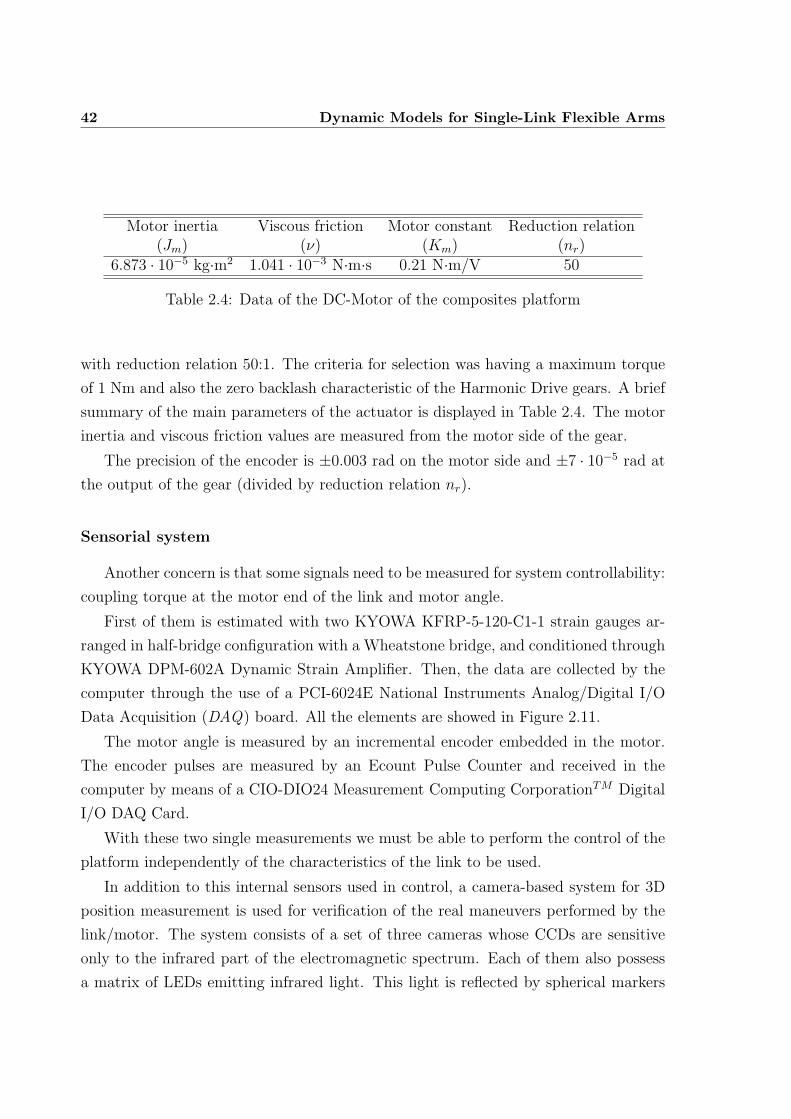
42 Dynamic Models for Single-Link Flexible Arms
Motor inertia Viscous friction Motor constant Reduction relation(Jm) (ν) (Km) (nr)
6.873 · 10−5 kg·m2 1.041 · 10−3 N·m·s 0.21 N·m/V 50
Table 2.4: Data of the DC-Motor of the composites platform
with reduction relation 50:1. The criteria for selection was having a maximum torque
of 1 Nm and also the zero backlash characteristic of the Harmonic Drive gears. A brief
summary of the main parameters of the actuator is displayed in Table 2.4. The motor
inertia and viscous friction values are measured from the motor side of the gear.
The precision of the encoder is ±0.003 rad on the motor side and ±7 · 10−5 rad at
the output of the gear (divided by reduction relation nr).
Sensorial system
Another concern is that some signals need to be measured for system controllability:
coupling torque at the motor end of the link and motor angle.
First of them is estimated with two KYOWA KFRP-5-120-C1-1 strain gauges ar-
ranged in half-bridge configuration with a Wheatstone bridge, and conditioned through
KYOWA DPM-602A Dynamic Strain Amplifier. Then, the data are collected by the
computer through the use of a PCI-6024E National Instruments Analog/Digital I/O
Data Acquisition (DAQ) board. All the elements are showed in Figure 2.11.
The motor angle is measured by an incremental encoder embedded in the motor.
The encoder pulses are measured by an Ecount Pulse Counter and received in the
computer by means of a CIO-DIO24 Measurement Computing CorporationTM Digital
I/O DAQ Card.
With these two single measurements we must be able to perform the control of the
platform independently of the characteristics of the link to be used.
In addition to this internal sensors used in control, a camera-based system for 3D
position measurement is used for verification of the real maneuvers performed by the
link/motor. The system consists of a set of three cameras whose CCDs are sensitive
only to the infrared part of the electromagnetic spectrum. Each of them also possess
a matrix of LEDs emitting infrared light. This light is reflected by spherical markers

2.6. Experimental platforms used for testing 43
Figure 2.11: Parts of the sensorial system: a) strain gauges; b) Wheatstone bridge; c)signal amplifier; and d) DAQ board
painted with a special material which intensely reflects the infrared light. The cameras
record the movement of the markers and, by means of triangulation, they are able
to obtain the spatial position of the markers in a previously calibrated environment.
Placing the markers at some strategic points of our system (typically the tip and the
base positions of the link) we can check the accuracy of our models and control systems.
The precision of this system for the volume of measurement (1.5× 2× 1 meters) is 0.3
mm.
Computer and software
The computer used for gathering the signal measurements and implementing the
different control schemes is a COMPAQ PC with Intel Processor Pentium III 650 MHz,
512MB of RAM and a 5GB hard disk.
Control schemes have been developed in MATLABTM 6.1 with the aid of Simulinkr
Toolbox 5.0. The models created have been compiled in MATLAB Real-Time Work-
shop (RTW) into a real-time environment running under Windows 2000.
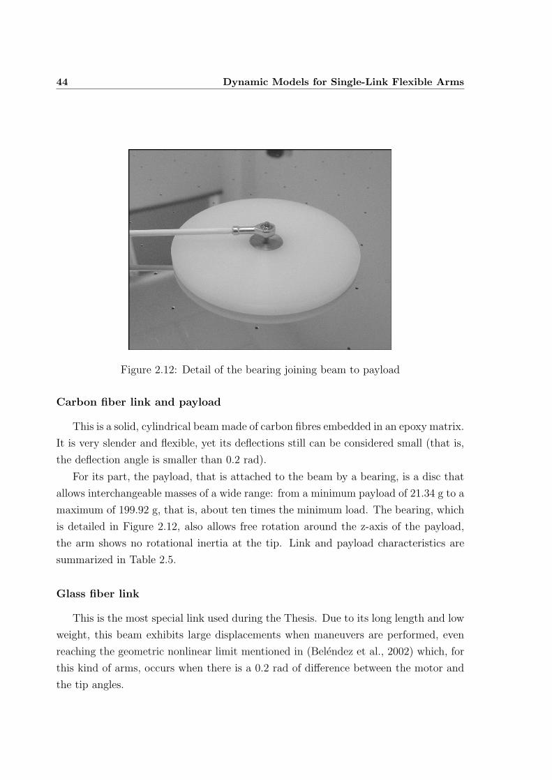
44 Dynamic Models for Single-Link Flexible Arms
Figure 2.12: Detail of the bearing joining beam to payload
Carbon fiber link and payload
This is a solid, cylindrical beam made of carbon fibres embedded in an epoxy matrix.
It is very slender and flexible, yet its deflections still can be considered small (that is,
the deflection angle is smaller than 0.2 rad).
For its part, the payload, that is attached to the beam by a bearing, is a disc that
allows interchangeable masses of a wide range: from a minimum payload of 21.34 g to a
maximum of 199.92 g, that is, about ten times the minimum load. The bearing, which
is detailed in Figure 2.12, also allows free rotation around the z-axis of the payload,
the arm shows no rotational inertia at the tip. Link and payload characteristics are
summarized in Table 2.5.
Glass fiber link
This is the most special link used during the Thesis. Due to its long length and low
weight, this beam exhibits large displacements when maneuvers are performed, even
reaching the geometric nonlinear limit mentioned in (Belendez et al., 2002) which, for
this kind of arms, occurs when there is a 0.2 rad of difference between the motor and
the tip angles.
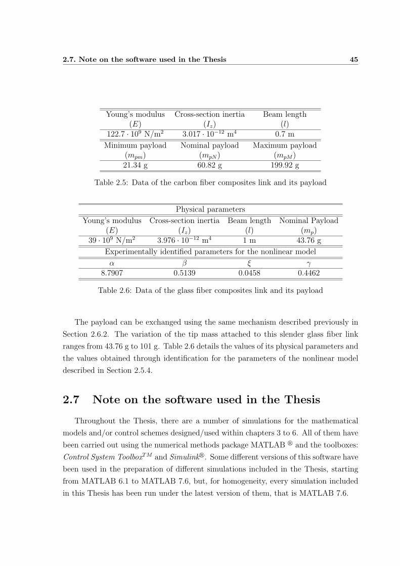
2.7. Note on the software used in the Thesis 45
Young’s modulus Cross-section inertia Beam length(E) (Iz) (l)
122.7 · 109 N/m2 3.017 · 10−12 m4 0.7 m
Minimum payload Nominal payload Maximum payload(mpm) (mpN) (mpM)21.34 g 60.82 g 199.92 g
Table 2.5: Data of the carbon fiber composites link and its payload
Physical parameters
Young’s modulus Cross-section inertia Beam length Nominal Payload(E) (Iz) (l) (mp)
39 · 109 N/m2 3.976 · 10−12 m4 1 m 43.76 g
Experimentally identified parameters for the nonlinear model
α β ξ γ8.7907 0.5139 0.0458 0.4462
Table 2.6: Data of the glass fiber composites link and its payload
The payload can be exchanged using the same mechanism described previously in
Section 2.6.2. The variation of the tip mass attached to this slender glass fiber link
ranges from 43.76 g to 101 g. Table 2.6 details the values of its physical parameters and
the values obtained through identification for the parameters of the nonlinear model
described in Section 2.5.4.
2.7 Note on the software used in the Thesis
Throughout the Thesis, there are a number of simulations for the mathematical
models and/or control schemes designed/used within chapters 3 to 6. All of them have
been carried out using the numerical methods package MATLAB r and the toolboxes:
Control System ToolboxTM and Simulinkr. Some different versions of this software have
been used in the preparation of different simulations included in the Thesis, starting
from MATLAB 6.1 to MATLAB 7.6, but, for homogeneity, every simulation included
in this Thesis has been run under the latest version of them, that is MATLAB 7.6.

46 Dynamic Models for Single-Link Flexible Arms
Chapter 3
Open loop control based on system
inversion
This Chapter presents a simple, low computational cost scheme for open-loop tra-
jectory tracking control of single link flexible manipulators. The control is performed
by direct dynamic inversion of the mathematical model of the system. This inversion is
non-causal, therefore it is necessary to calculate the trajectory beforehand in an off-line
stage. In addition, the trajectory needs to be differentiable the same number of times
as the order of the differential equation utilized for modeling.
Due to the particular characteristics of the trajectory needed for inversion, a family
of polynomial trajectories is defined in this Chapter. They depend on a small number of
parameters which are particular to the specifications (maneuver time, angle described)
or dependent on the physical limitations of the platform (acceleration and snap). They
also provide objective criteria for determining the parameters of the motor controller.
3.1 Problem description
The vibrations of flexible systems when they are performing movements are tightly
related with the reference signals that we provide to these structures. That is, if we
set a reference that is extremely demanding (e.g. a linear reference requiring a high
speed in a very short time or even a step input) for a mechanical system it results in
a motion exhibiting, almost surely, high overshoot and, most probably, some vibration
48 Open loop control based on system inversion
until we reach the target position of the system. Why does it happen?
Any text book in basic mechanics teaches that any real mechanical structure has,
as was exposed in the modeling Chapter, infinite vibration modes and, equally, infinite
vibration frequencies. Whenever a reference maneuver excites any of these frequencies,
a vibration appears in our system compromising its steadiness. Fortunately, we do
not need to take care about an infinite number of frequencies, as most of the high fre-
quencies vibrations are either negligible in amplitude or quickly damped by structural
properties. We just need to cancel/control/eliminate those frequencies too stubborn to
disappear naturally, that is, the lowest natural frequencies of the structure. Typically,
and depending on its nature, a flexible link (of the kind used in flexible robotics) can
exhibit from one up to three significant modes of vibration. Actually, the platforms
presented in this Thesis can be rigourously modeled with a single natural frequency,
and the target model for which the inputs are to be designed is the single mass lumped
model presented in Section 2.4.2.
3.1.1 Open loop control approach
Between the number of different control schemes that have been previously applied
to cancel the vibrations in flexible robotic arms, considerable attention has been de-
voted to the open loop control of this kind of systems. There exist two main approaches:
based on the inversion of the flexible arm dynamics (Bayo, 1988; Feliu and Rattan,
1999; Piazzi and Visioli, 2000) or on the adjustment of the input reference (Singer and
Seering, 1990; Pao, 1999; Zanasi and Morselli, 2002; Mohamed et al., 2006).
The first consists on passing the desired reference through a inverted system model
and obtaining and equivalent reference that, when is applied to the system, reverts (in
the output) to the initial desired reference. While conceptually simple, this scheme
needs a complete model of the system to be inverted and usually has any or various
of the following undesirable effects: it takes a considerable amount of resources if the
model is complex; or must be performed previously if the inversion is non causal (Piazzi
and Visioli, 2000); or needs of an undetermined time of computation if it follows an
iterative process (Bayo, 1988). The latter control strategy, often called input shaping,
is a technique based on generating adequate input references that inherently reduce
the oscillation of a flexible structure without needing a feedback control or needing it
3.1. Problem description 49
only for refinement. The main drawback of this method is that the command signal is
lengthened by an amount of time equal to the duration of the input shaper. Actually,
both apparently different methods are two sides of the same theory as shown in (Feliu
and Rattan, 1999).
Lately, a new, different approach, which follows an intuitive, simple, but unconven-
tional idea, called wave-echo control, has also been developed (O’Connor, 2006). This
strategy sets the first half of the maneuver to a predefined trajectory and measures
the actual motion performed by the manipulator. Then, the controller adjusts the
input reference for the second half to describe an ”echo” of that movement, which, to
some extent, includes the dynamics of the manipulator. While this method is model
free, inherently robust and achieves vibrationless point-to-point motion, the reference
tracking problem has not been addressed yet.
In present Chapter, a non-causal, dynamic inversion approach has been adopted.
The stability of a system inversion has been investigated since the 60’s, mainly in linear
multi-input multi-output (MIMO) systems (Silverman, 1969), or, in recent years, in
nonlinear systems also (Devasia and Paden, 1994; Marro and Piazzi, 1996). A relevant
concept that appears when dealing with invertibility of a system is the functional
reproducibility, meaning the capacity of reproducing an output from a suitable input
function, introduced in (Brockett and Mesarovic, 1965). This property has been the
subject to many studies when the construction of noncausal inverse is carried out in
presence of unstable zero dynamics (Marro and Piazzi, 1996). For the model adopted in
this Chapter, functional reproducibility is guaranteed because the model of the system
dynamics is scalar and minimum phase.
3.1.2 Influence of trajectories
The selection of an appropriate reference is crucial and has been studied in literature
a long time since (Bayo and Paden, 1987). The more demanding a trajectory is, the
wider is the range of frequencies that are excited when it is introduced to the system.
As an example, the step reference excites all vibration frequencies from zero to infinite.
Therefore, if a smooth (high continuity and differentiability) reference is provided to
the manipulator, the necessary control effort to canceling vibrations diminishes, as the
residual vibration remaining in the system is smaller.
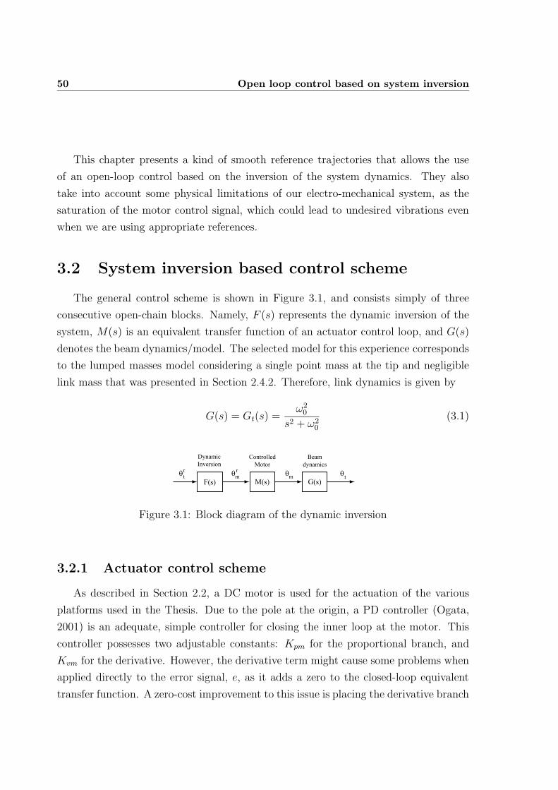
50 Open loop control based on system inversion
This chapter presents a kind of smooth reference trajectories that allows the use
of an open-loop control based on the inversion of the system dynamics. They also
take into account some physical limitations of our electro-mechanical system, as the
saturation of the motor control signal, which could lead to undesired vibrations even
when we are using appropriate references.
3.2 System inversion based control scheme
The general control scheme is shown in Figure 3.1, and consists simply of three
consecutive open-chain blocks. Namely, F (s) represents the dynamic inversion of the
system, M(s) is an equivalent transfer function of an actuator control loop, and G(s)
denotes the beam dynamics/model. The selected model for this experience corresponds
to the lumped masses model considering a single point mass at the tip and negligible
link mass that was presented in Section 2.4.2. Therefore, link dynamics is given by
G(s) = Gt(s) =ω20
s2 + ω20
(3.1)
M(s)t m m t
G(s)F(s)
Dynamic
Inversion
Controlled
Motor
Beam
dynamicsr rθ θ θ θ
Figure 3.1: Block diagram of the dynamic inversion
3.2.1 Actuator control scheme
As described in Section 2.2, a DC motor is used for the actuation of the various
platforms used in the Thesis. Due to the pole at the origin, a PD controller (Ogata,
2001) is an adequate, simple controller for closing the inner loop at the motor. This
controller possesses two adjustable constants: Kpm for the proportional branch, and
Kvm for the derivative. However, the derivative term might cause some problems when
applied directly to the error signal, e, as it adds a zero to the closed-loop equivalent
transfer function. A zero-cost improvement to this issue is placing the derivative branch
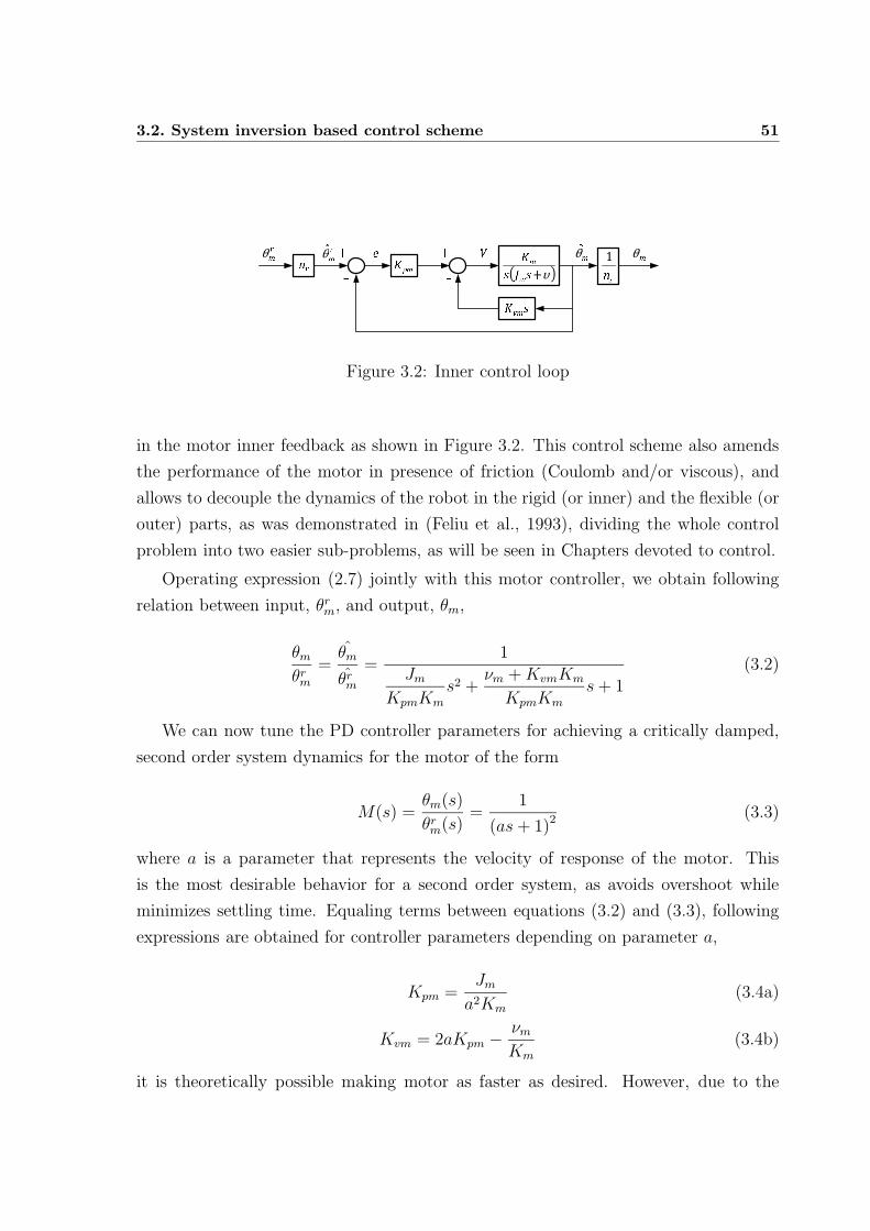
3.2. System inversion based control scheme 51V m m sJs Km m rnsK v mK p m rmn rrm eFigure 3.2: Inner control loop
in the motor inner feedback as shown in Figure 3.2. This control scheme also amends
the performance of the motor in presence of friction (Coulomb and/or viscous), and
allows to decouple the dynamics of the robot in the rigid (or inner) and the flexible (or
outer) parts, as was demonstrated in (Feliu et al., 1993), dividing the whole control
problem into two easier sub-problems, as will be seen in Chapters devoted to control.
Operating expression (2.7) jointly with this motor controller, we obtain following
relation between input, θrm, and output, θm,
θmθrm
=θm
θrm=
1
Jm
KpmKm
s2 +νm +KvmKm
KpmKm
s+ 1(3.2)
We can now tune the PD controller parameters for achieving a critically damped,
second order system dynamics for the motor of the form
M(s) =θm(s)
θrm(s)=
1
(as+ 1)2(3.3)
where a is a parameter that represents the velocity of response of the motor. This
is the most desirable behavior for a second order system, as avoids overshoot while
minimizes settling time. Equaling terms between equations (3.2) and (3.3), following
expressions are obtained for controller parameters depending on parameter a,
Kpm =Jm
a2Km
(3.4a)
Kvm = 2aKpm − νmKm
(3.4b)
it is theoretically possible making motor as faster as desired. However, due to the
52 Open loop control based on system inversion
physical limitations of the actuator that is a very unrealistic hypothesis.
Basing upon previous equations, it is theoretically possible to obtain a motor dy-
namics as fast as desired by simply making a → 0. However, that is a very unrealistic
hypothesis as it leads to very large controller gain Kpm, hence the controller demanding
high values of the control signal of the motor with the consequences of saturation and
malfunction of the motor. In Section 3.3.1 these physical constraints are incorporated
to the motor control design to obtain a realistic and reachable value a. Therefore, al-
though the motor dynamics can be made quite fast compared to that of the mechanical
part of the arm, in general, we cannot consider it negligible.
3.2.2 Noncausal dynamic inversion
The system inversion is performed easily by inverting the model transfer function
of the manipulator dynamics. Considering only the link dynamics, the inversion block
yields
Fb(s) = G−1t (s) =
s2 + ω20
ω20
(3.5)
Applying the inverse Laplace transform to Fb, the modified reference that must be
provided to the motor to cancel the vibration of the link can be calculated as
θrm(t) =1
ω20
θrt (t) + θrt (t) (3.6)
Equation (3.6) implies that θrt must be, at least, two times differentiable to obtain
a finite reference that achieves the desired vibrationless tracking of the reference.
However, even if this inversion cancels the beam vibration, still a perfect tracking is
not achieved, as the equivalent motor control loop dynamics introduces a (small) delay
in the response. This can be corrected if we include the equivalent transfer function
for the actuator control loop (3.3) in equation (3.5), resulting
Fs(s) = M−1(s)G−1t (s) = (1 + as)2
s2 + ω20
ω20
(3.7)
and, applying again the inverse Laplace
3.3. Constrained trajectory design 53
θrm(t) =a2
ω20
....θ
rt (t) +
2a
ω20
...θrt (t) +
(
a2 +1
ω20
)
θrt (t) + 2aθrt (t) + θrt (3.8)
Hence, achieving a perfect tracking of a desired trajectory is restricted to those
references that are four times differentiable.
3.3 Constrained trajectory design
We have finally defined the scenario which the trajectories must be defined for: a
flexible arm modeled as a second order system with two poles in the imaginary axis, as
given by equation (2.40), attached to a DC motor with an internal control loop con-
sisting of a PD controller which has two degrees of freedom for design (constants Kpm
and Kvm). The coupling between both attached systems has proven to be removable
by means of the compensation term shown in Figure 2.2.
These features determine the definitive form and coefficients of the trajectory equa-
tions as stated in following subsections.
3.3.1 Control signal saturation
A previous step to the definition of the trajectories, the possible saturation of the
control signal must be studied from a high-level point-of-view. Depending on the ref-
erence shape, the controller might demand to the motor very high control signals (that
is, unrealistic, high motor torques). However, due to the electromechanical limitations
of DC motors, the maximum torque that can be delivered, and, hence the input control
signal that can be provided to the motor has an upper limit. This constraint provides
us with a criterion for choosing appropriately the PD controller constants in order to
avoid saturations that cause the apparition of non-linearities. Thus, we divide the
capacity of the signal between the two main tasks we must consider to perform the
manoeuvre: firstly, the manoeuvre itself, as if the tracking were perfect; and secondly,
the correction of position errors due to perturbations. Therefore, we split our prob-
lem in other two which are simpler. From now on we will denote Vt as the maximum
amount of control signal dedicated to the trajectories, and Vp to the maximum amount
dedicated to correct errors such that Vmax = Vt + Vp.
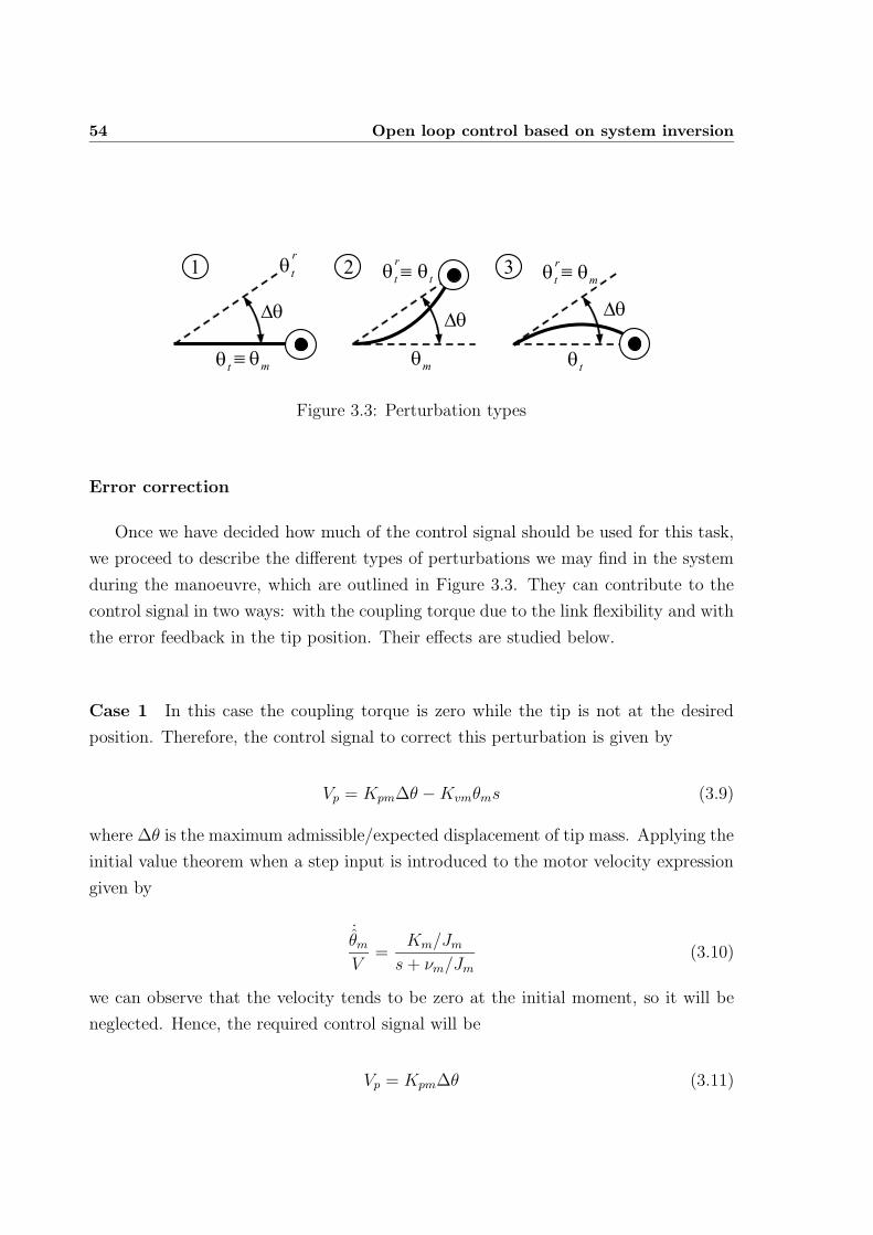
54 Open loop control based on system inversion
tθ
≡
θ∆
1 ≡2 ≡3
tθ
tθ
mθ
θ∆θ∆
tθ
tθ
mθ
mθ
tθ
rr
r
Figure 3.3: Perturbation types
Error correction
Once we have decided how much of the control signal should be used for this task,
we proceed to describe the different types of perturbations we may find in the system
during the manoeuvre, which are outlined in Figure 3.3. They can contribute to the
control signal in two ways: with the coupling torque due to the link flexibility and with
the error feedback in the tip position. Their effects are studied below.
Case 1 In this case the coupling torque is zero while the tip is not at the desired
position. Therefore, the control signal to correct this perturbation is given by
Vp = Kpm∆θ −Kvmθms (3.9)
where ∆θ is the maximum admissible/expected displacement of tip mass. Applying the
initial value theorem when a step input is introduced to the motor velocity expression
given by
˙θmV
=Km/Jm
s+ νm/Jm
(3.10)
we can observe that the velocity tends to be zero at the initial moment, so it will be
neglected. Hence, the required control signal will be
Vp = Kpm∆θ (3.11)
3.3. Constrained trajectory design 55
Case 2 The second kind of perturbation considered occurs when the bar is deflected
but the tip position is at the right place. In this case, the error e will be zero, and the
only contribution for correcting the perturbation will be given by the coupling torque
according to
Vp =c
Kmnr
∆θ (3.12)
Case 3 The last considered perturbation includes both effects: tip position error and
link deflection. Combining them, the expression for the control signal will be
Vp =
(
Kpm +c
Kmnr
)
∆θ (3.13)
where the velocity term has been again canceled for the aforementioned reason. It
seems quite obvious that it represents the worst case and, therefore, it is the only one
we need to consider.
3.3.2 Motor controller tuning
In equation (3.13), we have found objective criteria for calculating Kpm from the
control signal limitations. In addition, from the restriction proposed in Section 3.2.1,
equation (3.3), of adapting the motor to a critically damped system, a new restriction
for determining Kvm is introduced. Combining this requirement with equations (3.13)
and (3.4), we obtain the following equations for determining the controller parameters
Kpm =Vp
∆θ− c
Kmnr
(3.14a)
Kvm = 2
√JmKpm
Km
− ν
Km
(3.14b)
With these equations we have completed the design of our motor control system
guaranteeing that there will be no saturation in our control signal, and, therefore,
linearity in motor operation.
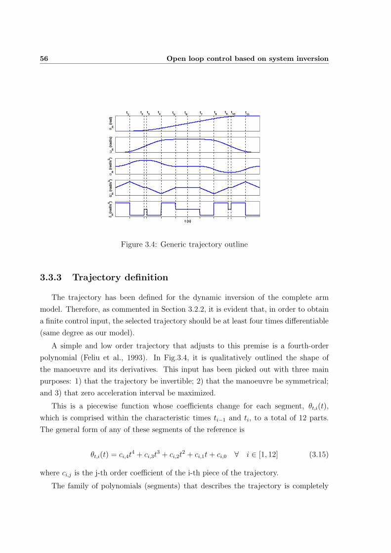
56 Open loop control based on system inversion
θ m (
rad)
ωm
(ra
d/s)
α m (
rad/
s2 )
α m (
rad/
s3 )
t (s)
δ m(r
ad/s
4 )t4 t
6t10
t8t
1t3 t
5t7
t9 t
11t2
⋅
Figure 3.4: Generic trajectory outline
3.3.3 Trajectory definition
The trajectory has been defined for the dynamic inversion of the complete arm
model. Therefore, as commented in Section 3.2.2, it is evident that, in order to obtain
a finite control input, the selected trajectory should be at least four times differentiable
(same degree as our model).
A simple and low order trajectory that adjusts to this premise is a fourth-order
polynomial (Feliu et al., 1993). In Fig.3.4, it is qualitatively outlined the shape of
the manoeuvre and its derivatives. This input has been picked out with three main
purposes: 1) that the trajectory be invertible; 2) that the manoeuvre be symmetrical;
and 3) that zero acceleration interval be maximized.
This is a piecewise function whose coefficients change for each segment, θt,i(t),
which is comprised within the characteristic times ti−1 and ti, to a total of 12 parts.
The general form of any of these segments of the reference is
θt,i(t) = ci,4t4 + ci,3t
3 + ci,2t2 + ci,1t+ ci,0 ∀ i ∈ [1, 12] (3.15)
where ci,j is the j-th order coefficient of the i-th piece of the trajectory.
The family of polynomials (segments) that describes the trajectory is completely
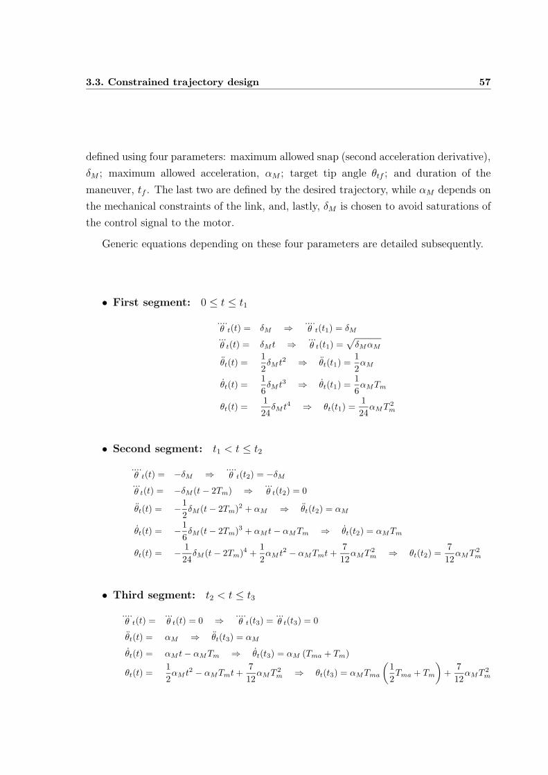
3.3. Constrained trajectory design 57
defined using four parameters: maximum allowed snap (second acceleration derivative),
δM ; maximum allowed acceleration, αM ; target tip angle θtf ; and duration of the
maneuver, tf . The last two are defined by the desired trajectory, while αM depends on
the mechanical constraints of the link, and, lastly, δM is chosen to avoid saturations of
the control signal to the motor.
Generic equations depending on these four parameters are detailed subsequently.
• First segment: 0 ≤ t ≤ t1
....θ t(t) = δM ⇒
....θ t(t1) = δM
...θ t(t) = δM t ⇒
...θ t(t1) =
√
δMαM
θt(t) =1
2δM t2 ⇒ θt(t1) =
1
2αM
θt(t) =1
6δM t3 ⇒ θt(t1) =
1
6αMTm
θt(t) =1
24δM t4 ⇒ θt(t1) =
1
24αMT 2
m
• Second segment: t1 < t ≤ t2
....θ t(t) = −δM ⇒
....θ t(t2) = −δM
...θ t(t) = −δM (t− 2Tm) ⇒
...θ t(t2) = 0
θt(t) = −1
2δM (t− 2Tm)2 + αM ⇒ θt(t2) = αM
θt(t) = −1
6δM (t− 2Tm)3 + αM t− αMTm ⇒ θt(t2) = αMTm
θt(t) = − 1
24δM (t− 2Tm)4 +
1
2αM t2 − αMTmt+
7
12αMT 2
m ⇒ θt(t2) =7
12αMT 2
m
• Third segment: t2 < t ≤ t3
....θ t(t) =
...θ t(t) = 0 ⇒
....θ t(t3) =
...θ t(t3) = 0
θt(t) = αM ⇒ θt(t3) = αM
θt(t) = αM t− αMTm ⇒ θt(t3) = αM (Tma + Tm)
θt(t) =1
2αM t2 − αMTmt+
7
12αMT 2
m ⇒ θt(t3) = αMTma
(1
2Tma + Tm
)
+7
12αMT 2
m
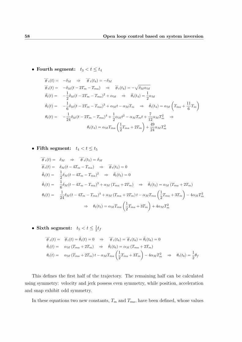
58 Open loop control based on system inversion
• Fourth segment: t3 < t ≤ t4
....θ t(t) = −δM ⇒
....θ t(t4) = −δM
...θ t(t) = −δM (t− 2Tm − Tma) ⇒
...θ t(t4) = −
√
δMαM
θt(t) = −1
2δM (t− 2Tm − Tma)
2 + αM ⇒ θt(t4) =1
2αM
θt(t) = −1
6δM (t− 2Tm − Tma)
3 + αM t− αMTm ⇒ θt(t4) = αM
(
Tma +11
6Tm
)
θt(t) = − 1
24δM (t− 2Tm − Tma)
4 +1
2αM t2 − αMTmt+
7
12αMT 2
m ⇒
θt(t4) = αMTma
(1
2Tma + 2Tm
)
+49
24αMT 2
m
• Fifth segment: t4 < t ≤ t5
....θ t(t) = δM ⇒
....θ t(t5) = δM
...θ t(t) = δM (t− 4Tm − Tma) ⇒
...θ t(t5) = 0
θt(t) =1
2δM (t− 4Tm − Tma)
2 ⇒ θt(t5) = 0
θt(t) =1
6δM (t− 4Tm − Tma)
3 + αM (Tma + 2Tm) ⇒ θt(t5) = αM (Tma + 2Tm)
θt(t) =1
24δM (t− 4Tm − Tma)
4 + αM (Tma + 2Tm) t− αMTma
(1
2Tma + 3Tm
)
− 4αMT 2
m
⇒ θt(t5) = αMTma
(1
2Tma + 3Tm
)
+ 4αMT 2
m
• Sixth segment: t5 < t ≤ 12tf
....θ t(t) =
...θ t(t) = θt(t) = 0 ⇒
....θ t(t6) =
...θ t(t6) = θt(t6) = 0
θt(t) = αM (Tma + 2Tm) ⇒ θt(t6) = αM (Tma + 2Tm)
θt(t) = αM (Tma + 2Tm) t− αMTma
(1
2Tma + 3Tm
)
− 4αMT 2
m ⇒ θt(t6) =1
2θf
This defines the first half of the trajectory. The remaining half can be calculated
using symmetry: velocity and jerk possess even symmetry, while position, acceleration
and snap exhibit odd symmetry.
In these equations two new constants, Tm and Tma, have been defined, whose values
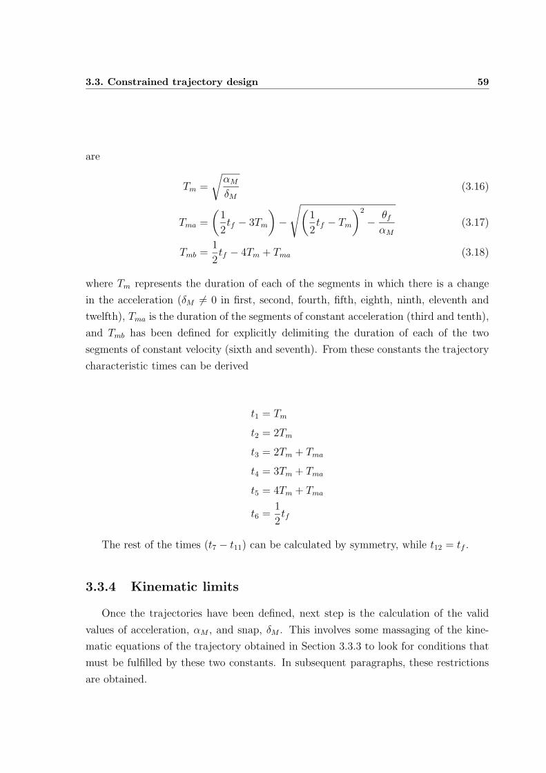
3.3. Constrained trajectory design 59
are
Tm =
√αM
δM(3.16)
Tma =
(1
2tf − 3Tm
)
−
√(1
2tf − Tm
)2
− θfαM
(3.17)
Tmb =1
2tf − 4Tm + Tma (3.18)
where Tm represents the duration of each of the segments in which there is a change
in the acceleration (δM 6= 0 in first, second, fourth, fifth, eighth, ninth, eleventh and
twelfth), Tma is the duration of the segments of constant acceleration (third and tenth),
and Tmb has been defined for explicitly delimiting the duration of each of the two
segments of constant velocity (sixth and seventh). From these constants the trajectory
characteristic times can be derived
t1 = Tm
t2 = 2Tm
t3 = 2Tm + Tma
t4 = 3Tm + Tma
t5 = 4Tm + Tma
t6 =1
2tf
The rest of the times (t7 − t11) can be calculated by symmetry, while t12 = tf .
3.3.4 Kinematic limits
Once the trajectories have been defined, next step is the calculation of the valid
values of acceleration, αM , and snap, δM . This involves some massaging of the kine-
matic equations of the trajectory obtained in Section 3.3.3 to look for conditions that
must be fulfilled by these two constants. In subsequent paragraphs, these restrictions
are obtained.
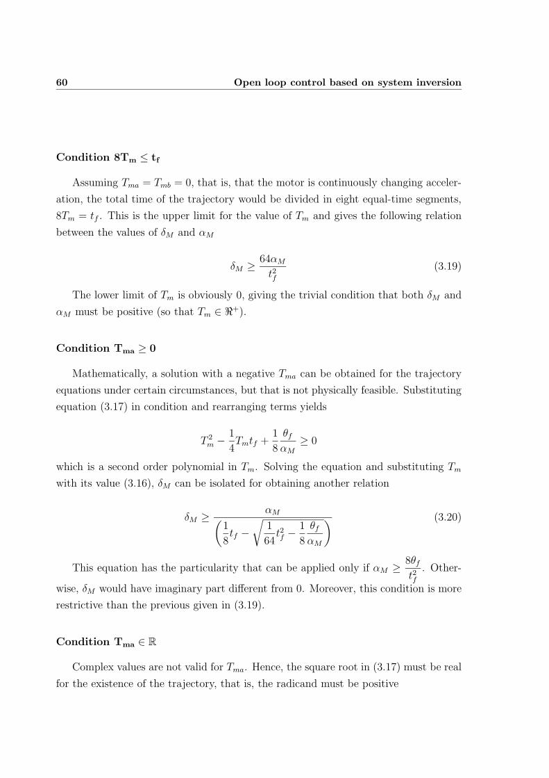
60 Open loop control based on system inversion
Condition 8Tm ≤ tf
Assuming Tma = Tmb = 0, that is, that the motor is continuously changing acceler-
ation, the total time of the trajectory would be divided in eight equal-time segments,
8Tm = tf . This is the upper limit for the value of Tm and gives the following relation
between the values of δM and αM
δM ≥ 64αM
t2f(3.19)
The lower limit of Tm is obviously 0, giving the trivial condition that both δM and
αM must be positive (so that Tm ∈ ℜ+).
Condition Tma ≥ 0
Mathematically, a solution with a negative Tma can be obtained for the trajectory
equations under certain circumstances, but that is not physically feasible. Substituting
equation (3.17) in condition and rearranging terms yields
T 2m − 1
4Tmtf +
1
8
θfαM
≥ 0
which is a second order polynomial in Tm. Solving the equation and substituting Tm
with its value (3.16), δM can be isolated for obtaining another relation
δM ≥ αM(1
8tf −
√1
64t2f −
1
8
θfαM
) (3.20)
This equation has the particularity that can be applied only if αM ≥ 8θft2f
. Other-
wise, δM would have imaginary part different from 0. Moreover, this condition is more
restrictive than the previous given in (3.19).
Condition Tma ∈ R
Complex values are not valid for Tma. Hence, the square root in (3.17) must be real
for the existence of the trajectory, that is, the radicand must be positive
3.3. Constrained trajectory design 61
(1
2tf − 3Tm
)2
− θfαM
≥ 0
Rearranging terms and clearing δM we obtain the following new restriction between
the values of acceleration and snap
δM ≥ αM(1
2tf −
√θfαM
)2 (3.21)
Under this limit, Tma is a complex number and the trajectory cannot be described.
Condition Tma ≤ 1
2tf − 4Tm
Tma is obviously limited by the total maneuver time and the time devoted to change
the acceleration. Again, substituting (3.16) and (3.17) and isolating the snap, the last
inequality is obtained, being
δM ≥ αM
t2f
(1
4t2f −
θfαM
) (3.22)
It can be proven that this equation is a stronger restriction than previous condition
Tma ∈ ℜ. It also has a vertical asymptote in
αM =4θft2f
(3.23)
that corresponds to the acceleration of a bang-bang profile that covers θf radians in tf
seconds. Below that acceleration limit, the trajectory cannot be performed.
3.3.5 Physical limits
These restrictions apply because of the physical limitations of the elements that
the manipulator consists of. Namely, the motor has an internal dynamics that, even
if can be noticeably quickened, cannot be neglected, and its signal control is bounded
depending on the speed and/or output torque that can supply; and the material of
62 Open loop control based on system inversion
the link, when subjected to bending moments surpassing its elastic limit, might suffer
permanent deformation.
Link material limit
This factor throws a limit for the maximum acceleration a material can experiment
without showing plastic deformation or excessive displacements at the tip. Depending
on if the material is metallic or composite, the calculations are different.
Metallic material In this case, the maximum acceleration allowed to the payload
is determined by the bending moment that we may reach in the bar before it exceeds
the elastic limit, which yields from the following expression (Berrocal, 2002)
σe =Mz
Izy (3.24)
being σe the elastic limit, Mz the bending moment, Iz the cross sectional inertia of the
beam, and y the distance between a point of the beam and its neutral axis.
On the other hand, the bending moment will be equal to the coupling torque in
equation (2.36). Then, if we substitute the maximum value admissible for Mz in the
equation and reorder terms, the following relation for the acceleration limit is obtained
αM =σeIz
ml2yM(3.25)
where yM represents the maximum distance to the neutral axis. In the case of a
cylindric beam, it corresponds to its radius.
Composite material When dealing with composites such as carbon or glass fibers,
the elastic limit has no meaning, as these materials remain elastic until they break.
Instead, these materials might enter in the large deflections zone, meaning that their ge-
ometry would be nonlinear (small deflections hypothesis being no longer valid). There-
fore, our acceleration limit will depend on this boundary. Directly from equation (2.36),
it yields
αM =c∆θMml2
(3.26)
3.3. Constrained trajectory design 63
where ∆θM is typically assumed to be 0.2 radians, as explained in (Belendez et al.,
2002).
Control signal limit
This value is slightly more difficult to obtain. First of all, we need to find where is
the maximum value reached by the control signal during the trajectory, which should
be smaller than the upper limit of the voltage supplied to the motor for avoiding
saturations in the control (which complicate the transfer function inversion). Because
of the fragmented nature of our expression for the reference we have, a priori, more than
one candidate. As a first approach, we calculate voltage reference at all the changes of
segment in the first half of the trajectory t1, t2, t3, t4 and t5. In the second half the
absolute value of the control signal demanded is smaller, as the viscous friction “helps”
the robot to decelerate.
The equation for the voltage, in terms of the desired trajectory, is obtained by apply-
ing the inverse Laplace transform to whole open loop model given by equation (2.42).
This operation yields
V (t) =nr
Kω20
(
Jm
....θ t(t) + ν
...θ t(t) + Jmω
20θt(t) + νω2
0 θt(t))
(3.27)
From here, and applying the correspondent values of θt and its derivatives as stated
in trajectory equations defined in Section 3.3.3, we obtain the equations for each value
of the voltage reference
V (t1) =nr
Km
(Jm
ω20
δM +ν
ω20
√
αMδM + Jm
1
2αM + ν
1
6αMTm
)
(3.28a)
V (t2) =nr
Km
(JmαM + ναMTm) (3.28b)
V (t3) =nr
Km
(JmαM + ναM (Tm + Tma)) (3.28c)
V (t4) =nr
Km
(Jm
ω20
δM − ν
ω20
√
αMδM + Jm
1
2αM + ν
1
6αM
(11
6Tm + Tma
))
(3.28d)
V (t5) =nr
Km
(Jm
ω20
δM + ναM (2Tm + Tma)
)
(3.28e)
64 Open loop control based on system inversion
The procedure is the following:
1. The smallest value of αM such that max V = Vt and the trajectory be feasible
is searched between the boundary couples (αM ,δM) obtained with the kinematic
restrictions (3.19) to (3.23).
2. A new value, greater than the previous by a desired step, is assigned to αM while
the reference voltage is set to Vt for each equation.
3. The resultant functions f(δM) are solved numerically (δM cannot be isolated in
some of the above expressions).
4. The minimum value among the five δM ’s is chosen as the maximum value of δM
that does not saturate the motor for the specified αM .
5. The process is repeated from step 2 until we calculate the desired interval of
accelerations, which can range from the smallest value obtained in step 1 to the
maximum admissible acceleration calculated in (3.25) or (3.26).
This procedure yields a numerical function δM (αM) that bounds the upper limit
of the feasibility region of pairs of values (δM , αM) that can be used for defining a
trajectory of the family previously described. This manner, any of the pairs within the
defined feasibility region avoids the undesirable effects listed in this Section: torques
and control signal are bounded within the limits and the trajectory equations fulfill
the required specifications.
3.4 Simulation results
The dynamic inversion scheme is here designed and studied in simulation for the
experimental platform defined in Section 2.6.2, (Flexible arm with composites link),
with the choice of a short carbon fiber link, in order to remain in the small displacements
(linear) zone, whose parameters can be found in Tables 2.4 and 2.5. Specifically, the
nominal payload used for simulations and experiments is mp = 60.82 · 10−3 kg.
In Section 3.3 we have described an objective method for determining both the
trajectories and the inner control loop of a flexible manipulator. To achieve this we
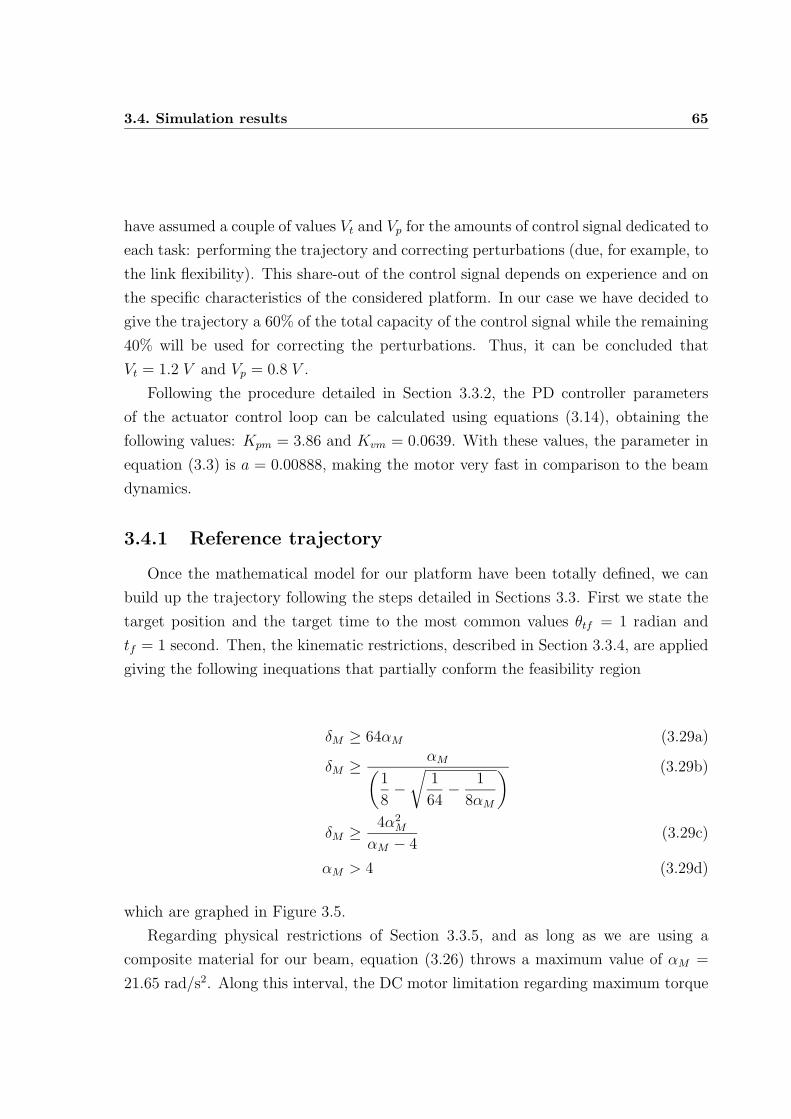
3.4. Simulation results 65
have assumed a couple of values Vt and Vp for the amounts of control signal dedicated to
each task: performing the trajectory and correcting perturbations (due, for example, to
the link flexibility). This share-out of the control signal depends on experience and on
the specific characteristics of the considered platform. In our case we have decided to
give the trajectory a 60% of the total capacity of the control signal while the remaining
40% will be used for correcting the perturbations. Thus, it can be concluded that
Vt = 1.2 V and Vp = 0.8 V .
Following the procedure detailed in Section 3.3.2, the PD controller parameters
of the actuator control loop can be calculated using equations (3.14), obtaining the
following values: Kpm = 3.86 and Kvm = 0.0639. With these values, the parameter in
equation (3.3) is a = 0.00888, making the motor very fast in comparison to the beam
dynamics.
3.4.1 Reference trajectory
Once the mathematical model for our platform have been totally defined, we can
build up the trajectory following the steps detailed in Sections 3.3. First we state the
target position and the target time to the most common values θtf = 1 radian and
tf = 1 second. Then, the kinematic restrictions, described in Section 3.3.4, are applied
giving the following inequations that partially conform the feasibility region
δM ≥ 64αM (3.29a)
δM ≥ αM(1
8−√
1
64− 1
8αM
) (3.29b)
δM ≥ 4α2M
αM − 4(3.29c)
αM > 4 (3.29d)
which are graphed in Figure 3.5.
Regarding physical restrictions of Section 3.3.5, and as long as we are using a
composite material for our beam, equation (3.26) throws a maximum value of αM =
21.65 rad/s2. Along this interval, the DC motor limitation regarding maximum torque
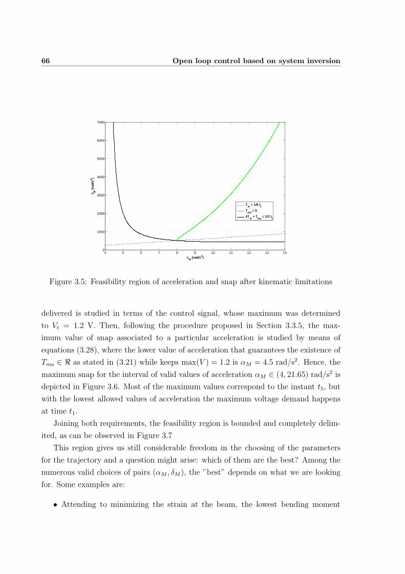
66 Open loop control based on system inversion
4 5 6 7 8 9 10 11 12 13 140
1000
2000
3000
4000
5000
6000
7000
αM
(rad/s 2)
δ M (
rad/
s4 )
Tm
≤ 1/8 tf
Tma
≥ 0
4Tm
+ Tma
≤ 1/2 tf
Figure 3.5: Feasibility region of acceleration and snap after kinematic limitations
delivered is studied in terms of the control signal, whose maximum was determined
to Vt = 1.2 V. Then, following the procedure proposed in Section 3.3.5, the max-
imum value of snap associated to a particular acceleration is studied by means of
equations (3.28), where the lower value of acceleration that guarantees the existence of
Tma ∈ ℜ as stated in (3.21) while keeps max(V ) = 1.2 is αM = 4.5 rad/s2. Hence, the
maximum snap for the interval of valid values of acceleration αM ∈ (4, 21.65) rad/s2 is
depicted in Figure 3.6. Most of the maximum values correspond to the instant t5, but
with the lowest allowed values of acceleration the maximum voltage demand happens
at time t1.
Joining both requirements, the feasibility region is bounded and completely delim-
ited, as can be observed in Figure 3.7
This region gives us still considerable freedom in the choosing of the parameters
for the trajectory and a question might arise: which of them are the best? Among the
numerous valid choices of pairs (αM , δM), the ”best” depends on what we are looking
for. Some examples are:
• Attending to minimizing the strain at the beam, the lowest bending moment
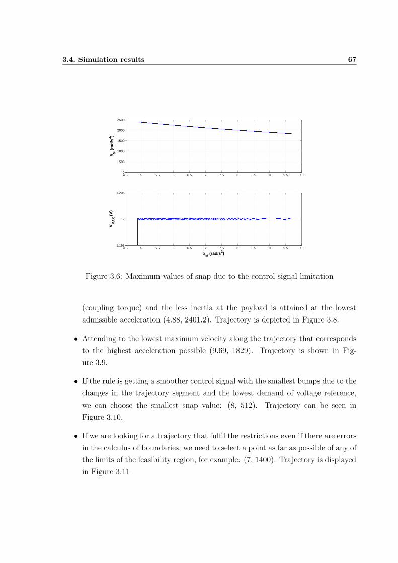
3.4. Simulation results 67
4.5 5 5.5 6 6.5 7 7.5 8 8.5 9 9.5 100
500
1000
1500
2000
2500
δ M (
rad/
s4 )
4.5 5 5.5 6 6.5 7 7.5 8 8.5 9 9.5 101.195
1.2
1.205
αM
(rad/s 2)
VM
AX
(V
)
Figure 3.6: Maximum values of snap due to the control signal limitation
(coupling torque) and the less inertia at the payload is attained at the lowest
admissible acceleration (4.88, 2401.2). Trajectory is depicted in Figure 3.8.
• Attending to the lowest maximum velocity along the trajectory that corresponds
to the highest acceleration possible (9.69, 1829). Trajectory is shown in Fig-
ure 3.9.
• If the rule is getting a smoother control signal with the smallest bumps due to the
changes in the trajectory segment and the lowest demand of voltage reference,
we can choose the smallest snap value: (8, 512). Trajectory can be seen in
Figure 3.10.
• If we are looking for a trajectory that fulfil the restrictions even if there are errors
in the calculus of boundaries, we need to select a point as far as possible of any of
the limits of the feasibility region, for example: (7, 1400). Trajectory is displayed
in Figure 3.11
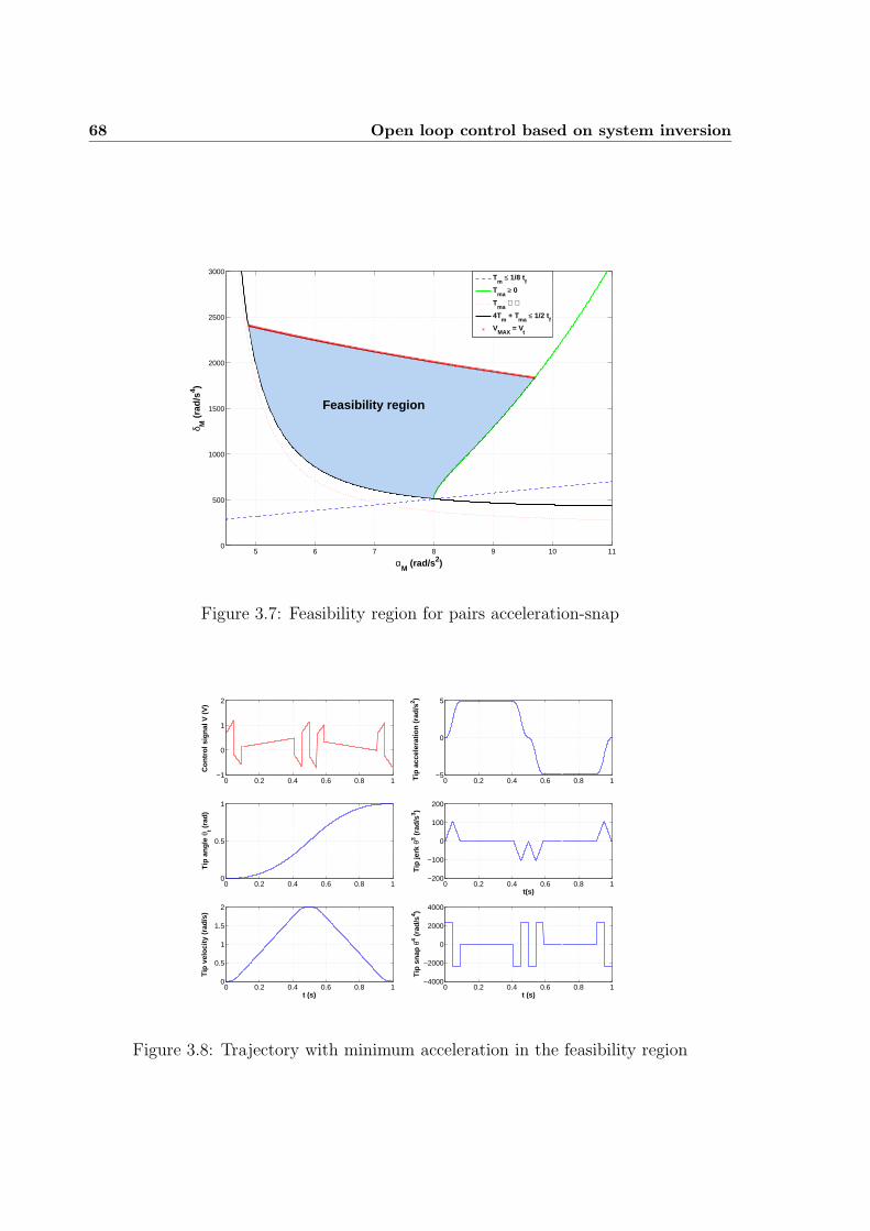
68 Open loop control based on system inversion
5 6 7 8 9 10 110
500
1000
1500
2000
2500
3000
αM
(rad/s 2)
δ M (
rad/
s4 )
T
m ≤ 1/8 t
f
Tma
≥ 0
Tma
∈ ℜ
4Tm
+ Tma
≤ 1/2 tf
VMAX
= Vt
Feasibility region
Figure 3.7: Feasibility region for pairs acceleration-snap
0 0.2 0.4 0.6 0.8 10
0.5
1
Tip
ang
le θ
t (ra
d)
0 0.2 0.4 0.6 0.8 10
0.5
1
1.5
2
Tip
vel
ocity
(ra
d/s)
t (s)
0 0.2 0.4 0.6 0.8 1−5
0
5
Tip
acc
eler
atio
n (r
ad/s
2 )
0 0.2 0.4 0.6 0.8 1−200
−100
0
100
200
t(s)
Tip
jerk
θ3 (
rad/
s3 )
0 0.2 0.4 0.6 0.8 1−4000
−2000
0
2000
4000
t (s)
Tip
sna
p θ4 (
rad/
s4 )
0 0.2 0.4 0.6 0.8 1−1
0
1
2
Con
trol
sig
nal V
(V
)
Figure 3.8: Trajectory with minimum acceleration in the feasibility region
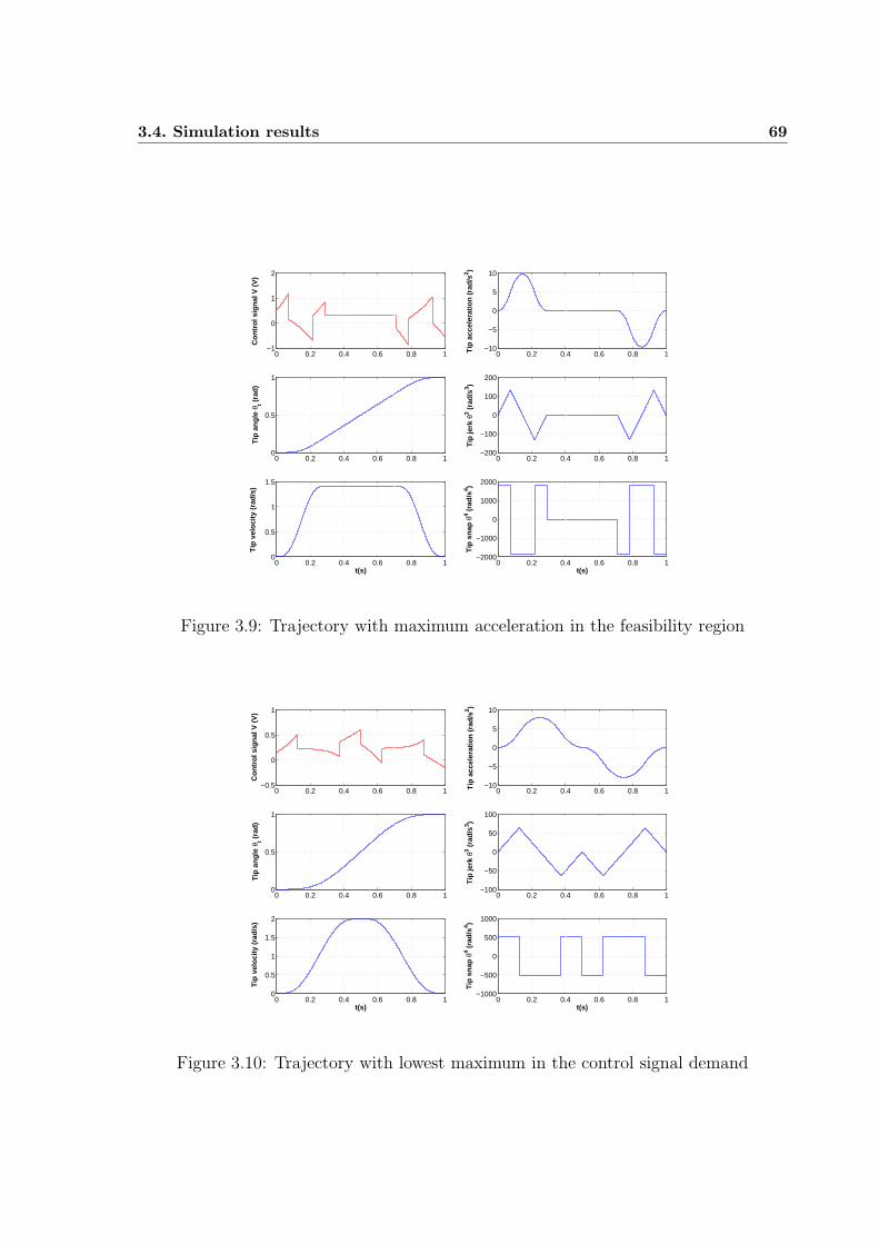
3.4. Simulation results 69
0 0.2 0.4 0.6 0.8 10
0.5
1
Tip
ang
le θ
t (ra
d)
0 0.2 0.4 0.6 0.8 10
0.5
1
1.5
t(s)
Tip
vel
ocity
(ra
d/s)
0 0.2 0.4 0.6 0.8 1−10
−5
0
5
10
Tip
acc
eler
atio
n (r
ad/s
2 )0 0.2 0.4 0.6 0.8 1
−200
−100
0
100
200
Tip
jerk
θ3 (
rad/
s3 )
0 0.2 0.4 0.6 0.8 1−2000
−1000
0
1000
2000
t(s)
Tip
sna
p θ4 (
rad/
s4 )
0 0.2 0.4 0.6 0.8 1−1
0
1
2
Con
trol
sig
nal V
(V
)
Figure 3.9: Trajectory with maximum acceleration in the feasibility region
0 0.2 0.4 0.6 0.8 10
0.5
1
Tip
ang
le θ
t (ra
d)
0 0.2 0.4 0.6 0.8 10
0.5
1
1.5
2
t(s)
Tip
vel
ocity
(ra
d/s)
0 0.2 0.4 0.6 0.8 1−10
−5
0
5
10
Tip
acc
eler
atio
n (r
ad/s
2 )
0 0.2 0.4 0.6 0.8 1−100
−50
0
50
100
Tip
jerk
θ3 (
rad/
s3 )
0 0.2 0.4 0.6 0.8 1−1000
−500
0
500
1000
t(s)
Tip
sna
p θ4 (
rad/
s4 )
0 0.2 0.4 0.6 0.8 1−0.5
0
0.5
1
Con
trol
sig
nal V
(V
)
Figure 3.10: Trajectory with lowest maximum in the control signal demand
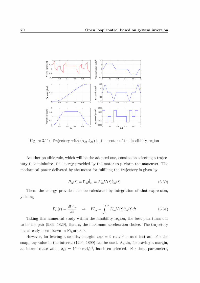
70 Open loop control based on system inversion
0 0.2 0.4 0.6 0.8 10
0.5
1
Tip
ang
le θ
t (ra
d)
0 0.2 0.4 0.6 0.8 10
0.5
1
1.5
2
t(s)
Tip
vel
ocity
(ra
d/s)
0 0.2 0.4 0.6 0.8 1−10
−5
0
5
10
Tip
acc
eler
atio
n (r
ad/s
2 )
0 0.2 0.4 0.6 0.8 1−100
−50
0
50
100
Tip
jerk
θ3 (
rad/
s3 )
0 0.2 0.4 0.6 0.8 1−2000
−1000
0
1000
2000
t(s)
Tip
sna
p θ4 (
rad/
s4 )
0 0.2 0.4 0.6 0.8 1−1
−0.5
0
0.5
1
Con
trol
sig
nal V
(V
)
Figure 3.11: Trajectory with (αM ,δM) in the center of the feasibility region
Another possible rule, which will be the adopted one, consists on selecting a trajec-
tory that minimizes the energy provided by the motor to perform the maneuver. The
mechanical power delivered by the motor for fulfilling the trajectory is given by
Pm(t) = Γmθm = KmV (t)θm(t) (3.30)
Then, the energy provided can be calculated by integration of that expression,
yielding
Pm(t) =dWm
dt⇒ Wm =
∫ tf
0
KmV (t)θm(t)dt (3.31)
Taking this numerical study within the feasibility region, the best pick turns out
to be the pair (9.69, 1829), that is, the maximum acceleration choice. The trajectory
has already been drawn in Figure 3.9.
However, for leaving a security margin, αM = 9 rad/s2 is used instead. For the
snap, any value in the interval (1296, 1899) can be used. Again, for leaving a margin,
an intermediate value, δM = 1600 rad/s4, has been selected. For these parameters,
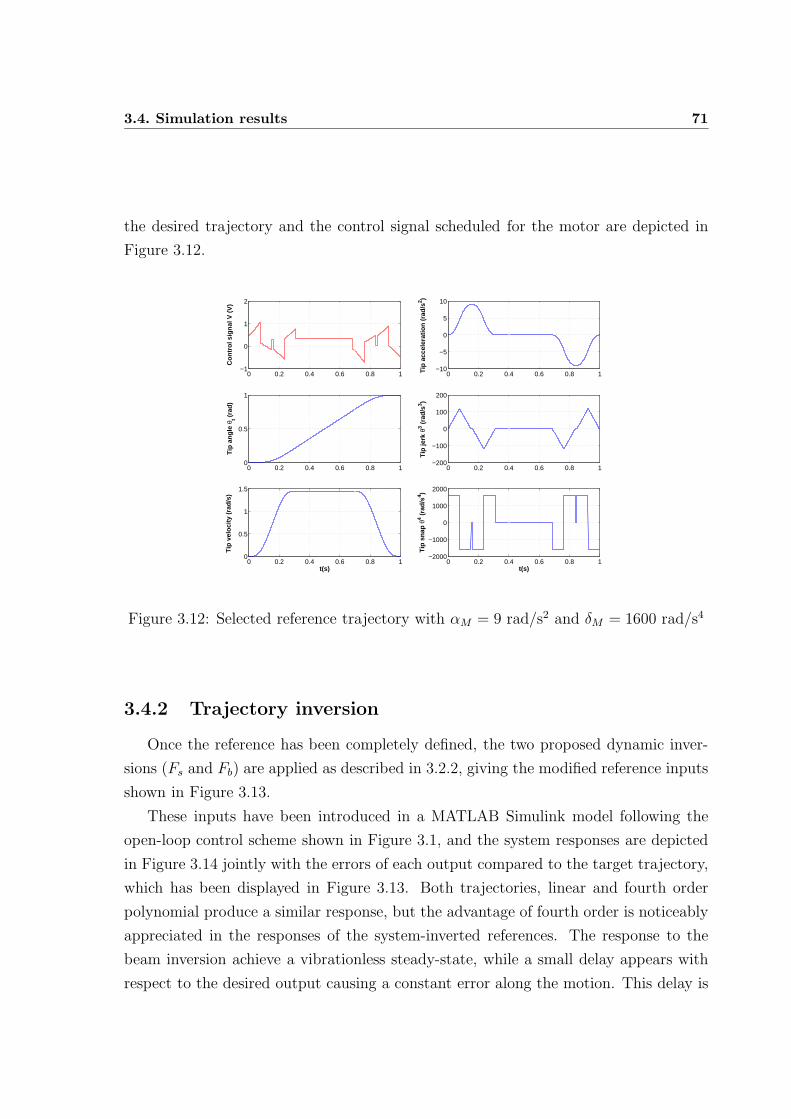
3.4. Simulation results 71
the desired trajectory and the control signal scheduled for the motor are depicted in
Figure 3.12.
0 0.2 0.4 0.6 0.8 10
0.5
1
Tip
ang
le θ
t (ra
d)
0 0.2 0.4 0.6 0.8 10
0.5
1
1.5
t(s)
Tip
vel
ocity
(ra
d/s)
0 0.2 0.4 0.6 0.8 1−10
−5
0
5
10
Tip
acc
eler
atio
n (r
ad/s
2 )
0 0.2 0.4 0.6 0.8 1−200
−100
0
100
200
Tip
jerk
θ3 (
rad/
s3 )
0 0.2 0.4 0.6 0.8 1−2000
−1000
0
1000
2000
t(s)
Tip
sna
p θ4 (
rad/
s4 )
0 0.2 0.4 0.6 0.8 1−1
0
1
2
Con
trol
sig
nal V
(V
)
Figure 3.12: Selected reference trajectory with αM = 9 rad/s2 and δM = 1600 rad/s4
3.4.2 Trajectory inversion
Once the reference has been completely defined, the two proposed dynamic inver-
sions (Fs and Fb) are applied as described in 3.2.2, giving the modified reference inputs
shown in Figure 3.13.
These inputs have been introduced in a MATLAB Simulink model following the
open-loop control scheme shown in Figure 3.1, and the system responses are depicted
in Figure 3.14 jointly with the errors of each output compared to the target trajectory,
which has been displayed in Figure 3.13. Both trajectories, linear and fourth order
polynomial produce a similar response, but the advantage of fourth order is noticeably
appreciated in the responses of the system-inverted references. The response to the
beam inversion achieve a vibrationless steady-state, while a small delay appears with
respect to the desired output causing a constant error along the motion. This delay is
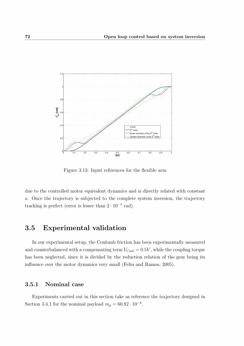
72 Open loop control based on system inversion
0 0.1 0.2 0.3 0.4 0.5 0.6 0.7 0.8 0.9 10
0.2
0.4
0.6
0.8
1
1.2
t(s)
θ mr (
rad)
Linear
4th order
Beam inversion of the 4th order
System inversion of the 4th order
Figure 3.13: Input references for the flexible arm
due to the controlled motor equivalent dynamics and is directly related with constant
a. Once the trajectory is subjected to the complete system inversion, the trajectory
tracking is perfect (error is lesser than 2 · 10−5 rad).
3.5 Experimental validation
In our experimental setup, the Coulomb friction has been experimentally measured
and counterbalanced with a compensating term VCoul = 0.5V , while the coupling torque
has been neglected, since it is divided by the reduction relation of the gear being its
influence over the motor dynamics very small (Feliu and Ramos, 2005).
3.5.1 Nominal case
Experiments carried out in this section take as reference the trajectory designed in
Section 3.4.1 for the nominal payload mp = 60.82 · 10−3.
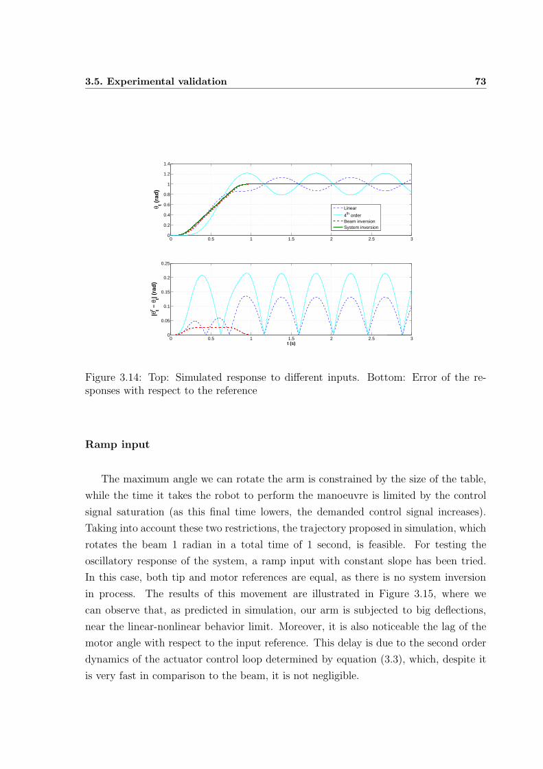
3.5. Experimental validation 73
0 0.5 1 1.5 2 2.5 30
0.2
0.4
0.6
0.8
1
1.2
1.4
θ t (ra
d)
0 0.5 1 1.5 2 2.5 30
0.05
0.1
0.15
0.2
0.25
t (s)
|θtr −
θt| (
rad)
Linear
4th orderBeam inversionSystem inversion
Figure 3.14: Top: Simulated response to different inputs. Bottom: Error of the re-sponses with respect to the reference
Ramp input
The maximum angle we can rotate the arm is constrained by the size of the table,
while the time it takes the robot to perform the manoeuvre is limited by the control
signal saturation (as this final time lowers, the demanded control signal increases).
Taking into account these two restrictions, the trajectory proposed in simulation, which
rotates the beam 1 radian in a total time of 1 second, is feasible. For testing the
oscillatory response of the system, a ramp input with constant slope has been tried.
In this case, both tip and motor references are equal, as there is no system inversion
in process. The results of this movement are illustrated in Figure 3.15, where we
can observe that, as predicted in simulation, our arm is subjected to big deflections,
near the linear-nonlinear behavior limit. Moreover, it is also noticeable the lag of the
motor angle with respect to the input reference. This delay is due to the second order
dynamics of the actuator control loop determined by equation (3.3), which, despite it
is very fast in comparison to the beam, it is not negligible.
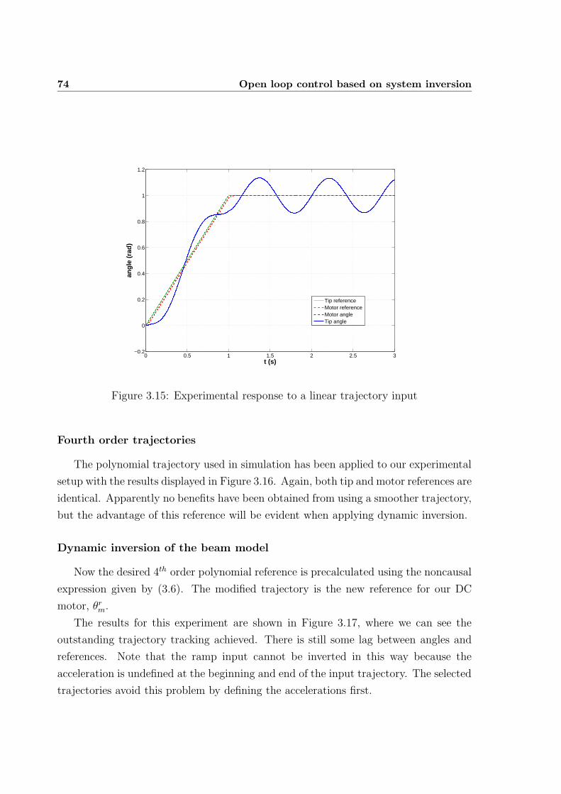
74 Open loop control based on system inversion
0 0.5 1 1.5 2 2.5 3−0.2
0
0.2
0.4
0.6
0.8
1
1.2
angl
e (r
ad)
t (s)
Tip referenceMotor referenceMotor angleTip angle
Figure 3.15: Experimental response to a linear trajectory input
Fourth order trajectories
The polynomial trajectory used in simulation has been applied to our experimental
setup with the results displayed in Figure 3.16. Again, both tip and motor references are
identical. Apparently no benefits have been obtained from using a smoother trajectory,
but the advantage of this reference will be evident when applying dynamic inversion.
Dynamic inversion of the beam model
Now the desired 4th order polynomial reference is precalculated using the noncausal
expression given by (3.6). The modified trajectory is the new reference for our DC
motor, θrm.
The results for this experiment are shown in Figure 3.17, where we can see the
outstanding trajectory tracking achieved. There is still some lag between angles and
references. Note that the ramp input cannot be inverted in this way because the
acceleration is undefined at the beginning and end of the input trajectory. The selected
trajectories avoid this problem by defining the accelerations first.
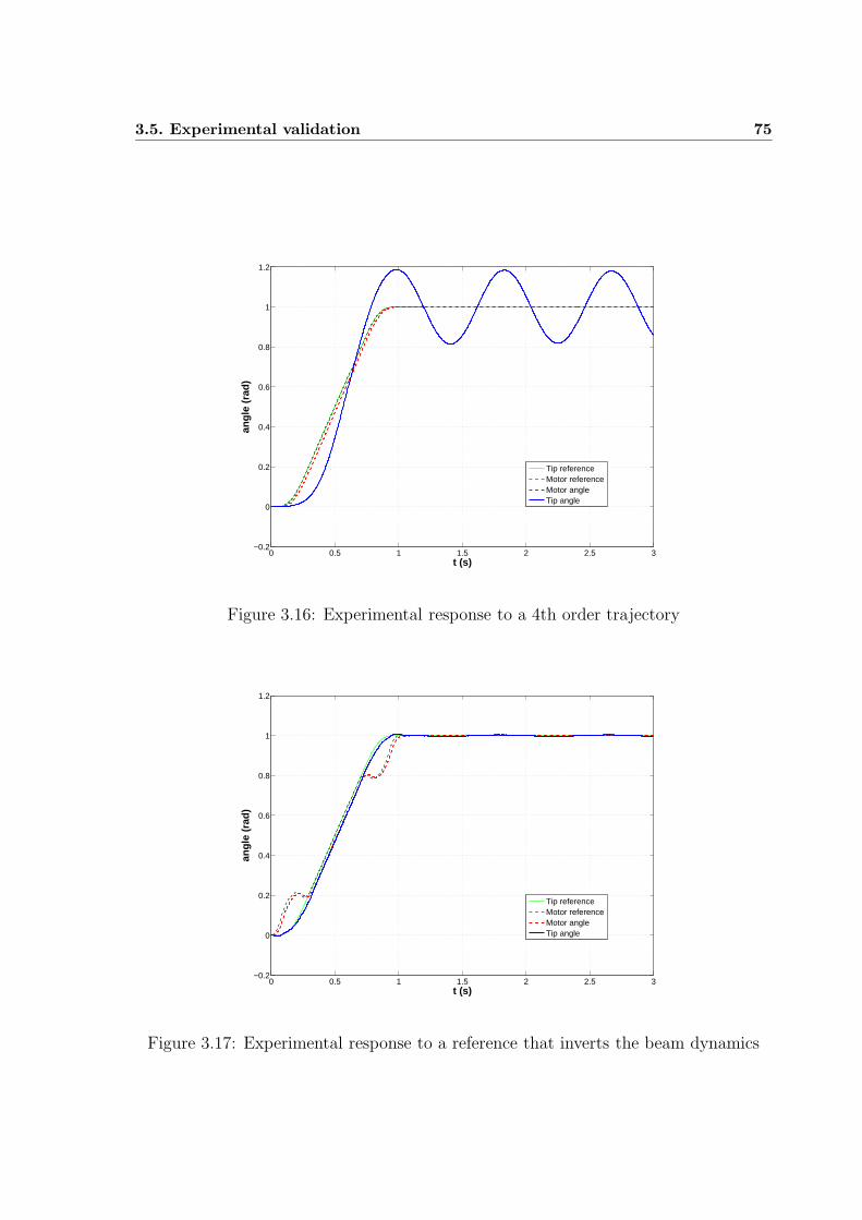
3.5. Experimental validation 75
0 0.5 1 1.5 2 2.5 3−0.2
0
0.2
0.4
0.6
0.8
1
1.2
angl
e (r
ad)
t (s)
Tip referenceMotor referenceMotor angleTip angle
Figure 3.16: Experimental response to a 4th order trajectory
0 0.5 1 1.5 2 2.5 3−0.2
0
0.2
0.4
0.6
0.8
1
1.2
angl
e (r
ad)
t (s)
Tip referenceMotor referenceMotor angleTip angle
Figure 3.17: Experimental response to a reference that inverts the beam dynamics
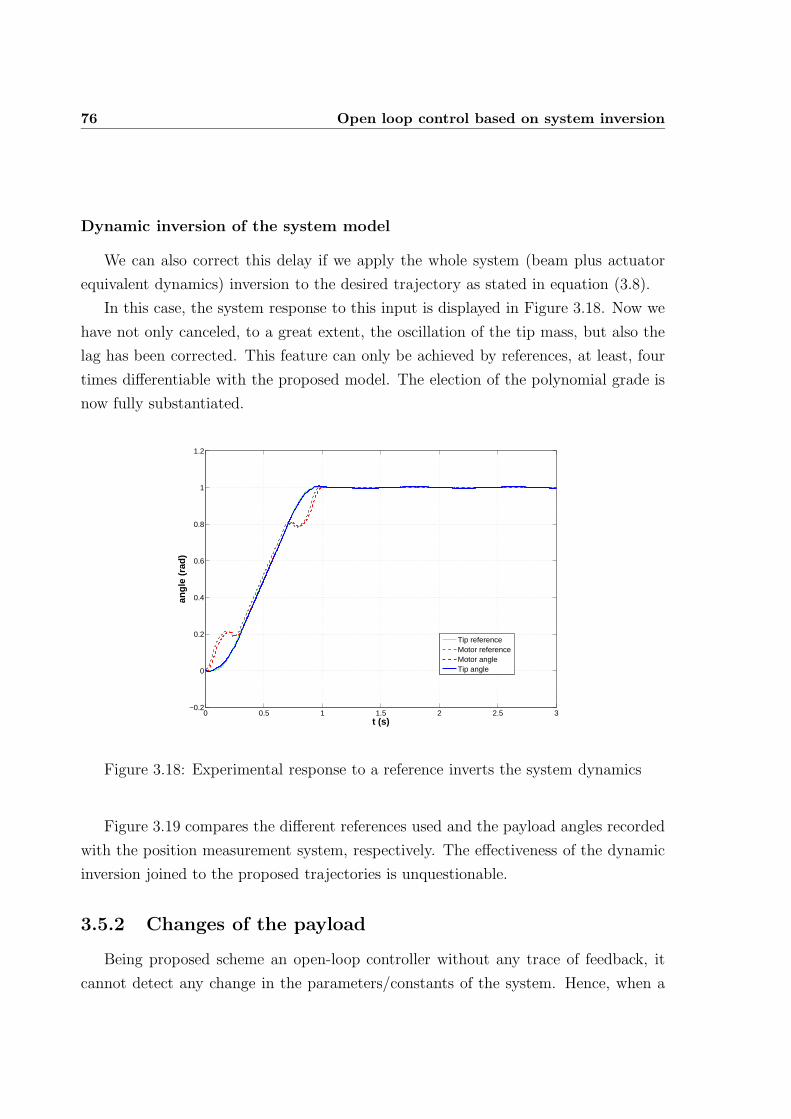
76 Open loop control based on system inversion
Dynamic inversion of the system model
We can also correct this delay if we apply the whole system (beam plus actuator
equivalent dynamics) inversion to the desired trajectory as stated in equation (3.8).
In this case, the system response to this input is displayed in Figure 3.18. Now we
have not only canceled, to a great extent, the oscillation of the tip mass, but also the
lag has been corrected. This feature can only be achieved by references, at least, four
times differentiable with the proposed model. The election of the polynomial grade is
now fully substantiated.
0 0.5 1 1.5 2 2.5 3−0.2
0
0.2
0.4
0.6
0.8
1
1.2
angl
e (r
ad)
t (s)
Tip referenceMotor referenceMotor angleTip angle
Figure 3.18: Experimental response to a reference inverts the system dynamics
Figure 3.19 compares the different references used and the payload angles recorded
with the position measurement system, respectively. The effectiveness of the dynamic
inversion joined to the proposed trajectories is unquestionable.
3.5.2 Changes of the payload
Being proposed scheme an open-loop controller without any trace of feedback, it
cannot detect any change in the parameters/constants of the system. Hence, when a
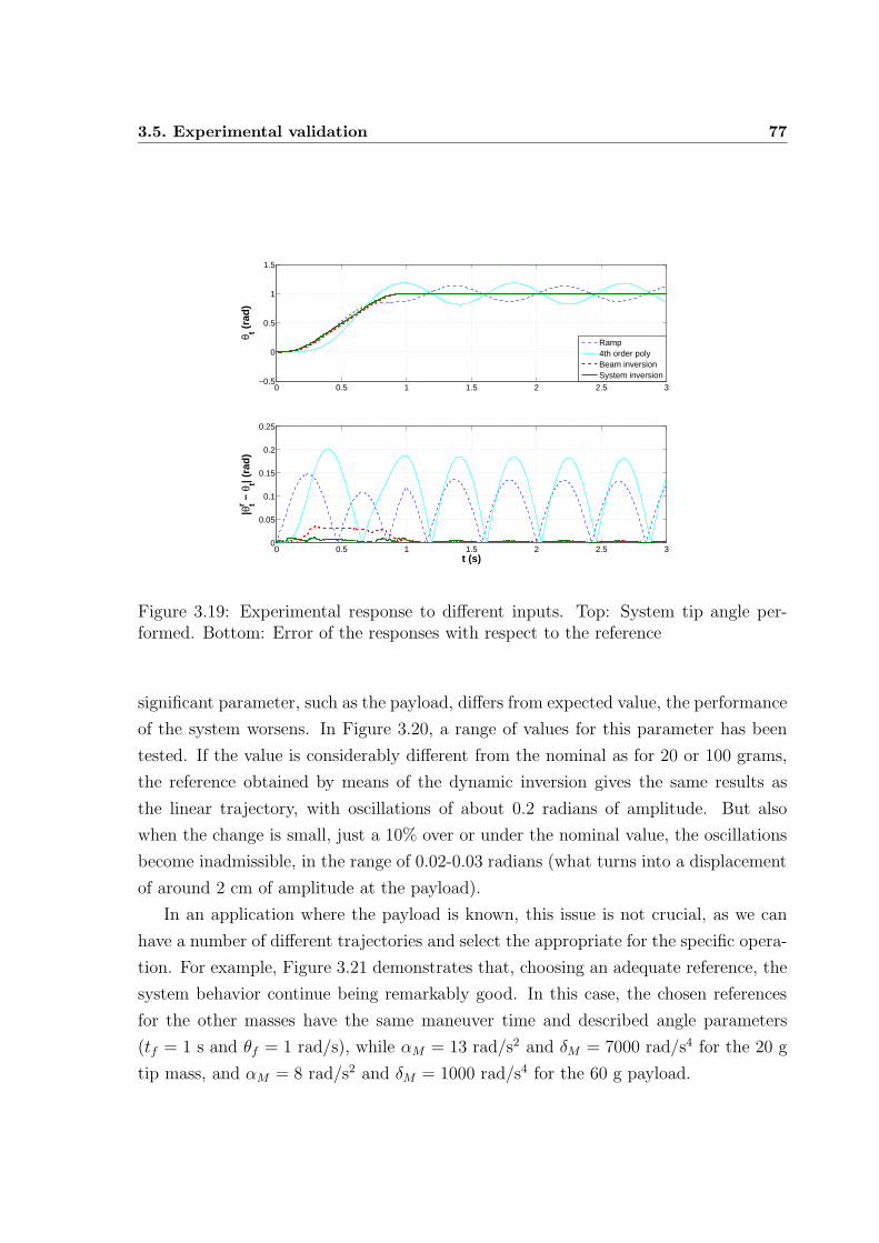
3.5. Experimental validation 77
0 0.5 1 1.5 2 2.5 3−0.5
0
0.5
1
1.5
θ t (ra
d)
0 0.5 1 1.5 2 2.5 30
0.05
0.1
0.15
0.2
0.25
t (s)
|θtr −
θt| (
rad)
Ramp4th order polyBeam inversionSystem inversion
Figure 3.19: Experimental response to different inputs. Top: System tip angle per-formed. Bottom: Error of the responses with respect to the reference
significant parameter, such as the payload, differs from expected value, the performance
of the system worsens. In Figure 3.20, a range of values for this parameter has been
tested. If the value is considerably different from the nominal as for 20 or 100 grams,
the reference obtained by means of the dynamic inversion gives the same results as
the linear trajectory, with oscillations of about 0.2 radians of amplitude. But also
when the change is small, just a 10% over or under the nominal value, the oscillations
become inadmissible, in the range of 0.02-0.03 radians (what turns into a displacement
of around 2 cm of amplitude at the payload).
In an application where the payload is known, this issue is not crucial, as we can
have a number of different trajectories and select the appropriate for the specific opera-
tion. For example, Figure 3.21 demonstrates that, choosing an adequate reference, the
system behavior continue being remarkably good. In this case, the chosen references
for the other masses have the same maneuver time and described angle parameters
(tf = 1 s and θf = 1 rad/s), while αM = 13 rad/s2 and δM = 7000 rad/s4 for the 20 g
tip mass, and αM = 8 rad/s2 and δM = 1000 rad/s4 for the 60 g payload.
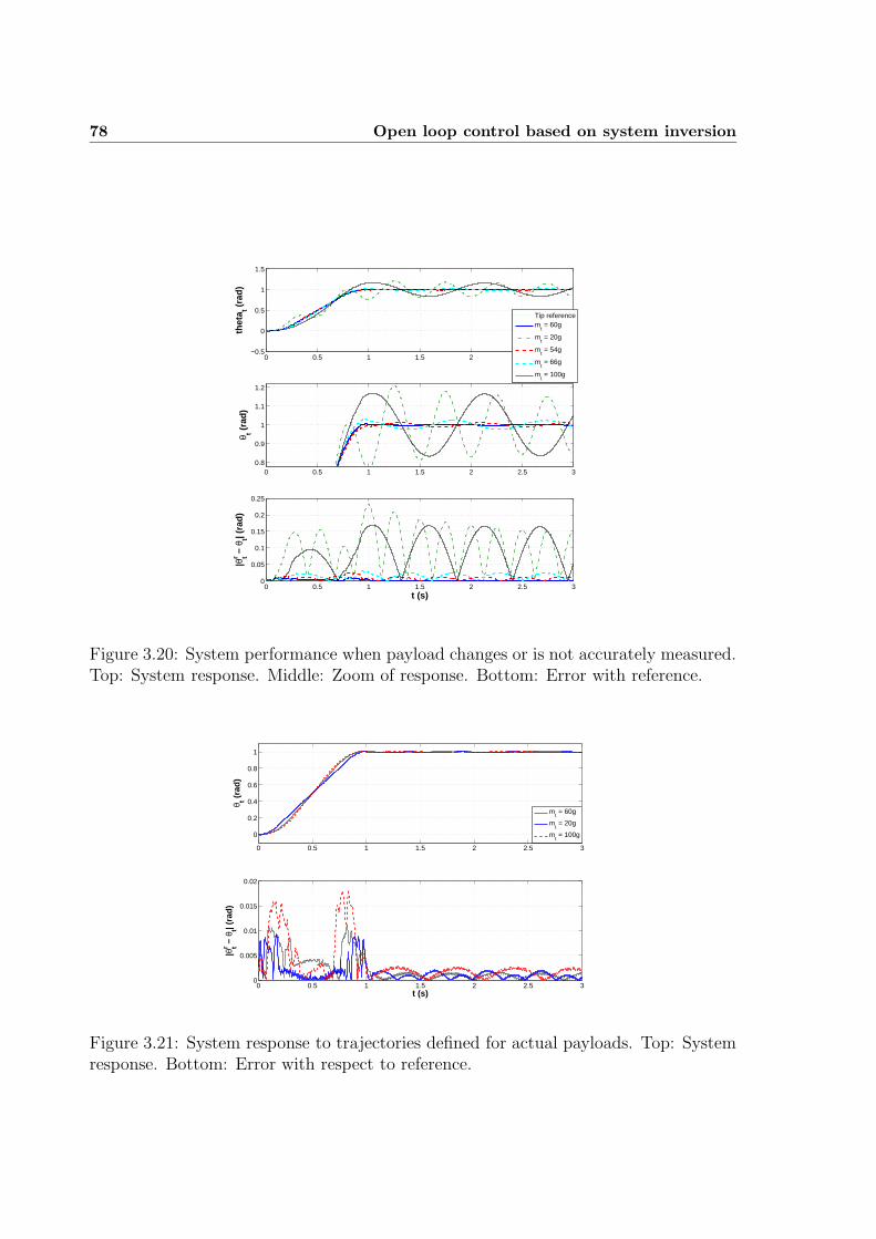
78 Open loop control based on system inversion
0 0.5 1 1.5 2 2.5 3−0.5
0
0.5
1
1.5
thet
at (
rad)
Tip referencem
t = 60g
mt = 20g
mt = 54g
mt = 66g
mt = 100g
0 0.5 1 1.5 2 2.5 30.8
0.9
1
1.1
1.2
θ t (ra
d)
0 0.5 1 1.5 2 2.5 30
0.05
0.1
0.15
0.2
0.25
|θtr −
θt| (
rad)
t (s)
Figure 3.20: System performance when payload changes or is not accurately measured.Top: System response. Middle: Zoom of response. Bottom: Error with reference.
0 0.5 1 1.5 2 2.5 3
0
0.2
0.4
0.6
0.8
1
θ t (ra
d)
mt = 60g
mt = 20g
mt = 100g
0 0.5 1 1.5 2 2.5 30
0.005
0.01
0.015
0.02
|θtr −
θt| (
rad)
t (s)
Figure 3.21: System response to trajectories defined for actual payloads. Top: Systemresponse. Bottom: Error with respect to reference.
3.6. Summary and conclusions 79
3.6 Summary and conclusions
This chapter presented an open-loop, noncausal dynamic inversion control scheme
based on the precalculation of a modified input that, when applied to the system,
provides the desired trajectory in the output. This direct, easy inversion has been
feasible because of the simplicity of the model used for describing the robot, which is
scalar and minimum phase.
In addition, a family of piecewise, 4th order polynomial trajectories that are suit-
able for dynamic inversion in simple, lumped masses models of flexible arms has been
developed. The order of the polynomial is in concordance with the relative order of the
manipulator model. Only four parameters need to be specified for defining the maneu-
ver during the design, namely, time, angle, maximum acceleration and maximum snap.
An objective process has been provided for calculating those maximums depending on
the physical constraints of the system, and also the actuator controller constants.
The open-loop dynamic inversion has been tested on a flexible arm with a carbon
fiber link. Despite its simplicity, the control scheme has provided superb experimental
results with very little computation effort. Simply by using a previously calculated off-
line stage to produce a modified input which provides perfect tracking of the desired
trajectory.
However, these open-loop schemes prove to be very sensitive to uncertainties in the
system parameters, degrading the performance abruptly when a change is introduced
in the system. An experimental example has been performed with different payloads
where the system has behaved as expected. To maintain the optimal performance, we
would need to know in advance the mass so we could switch to the adequate reference
for tracking the original reference.
Evidently, in the pursuit of controllers whose performance is not affected by changes
in the parameters of the system, we need to know how good is the system output dur-
ing maneuvers. Therefore, the necessity of closed-loop schemes that intelligently take
advantage of the sensorial system in a feedback loop is unquestionable, and motivates
the development of the robust/adaptive controllers described in following Chapters.

80 Open loop control based on system inversion
Chapter 4
Robust control
4.1 Introduction
In the previous Chapter, the vibrationless motion of a flexible manipulator was
achieved by a dynamic inversion based open-loop controller. While simple, this scheme
is very sensitive to any changes in the plant, such as the variation of the tip mass,
and depends strongly on the exact modeling of the mechanical system. Any change
in the plant parameters reduces the controller performance, making the system lose
the desired specifications. Actually, the payload, which is one of the most determinant
parameters in robot dynamics, may change very often in a robotic system under normal
operation, either when changing the tip tool being used, or when grasping an object
with non negligible weight.
A number of different strategies, which can be grouped into three big categories of
control theory, have been applied to overcome this drawback. Namely, intelligent con-
trol, based on techniques with the ability to learn, such as neural networks or genetic
algorithms, which are usually very demanding computationally due to its nonlinear
intrinsic nature; robust control, e.g. H∞ control, which provides schemes that perform
correctly under a range of parameter uncertainties; and adaptive control, which pro-
vides controllers that are capable of adjusting their values depending on some criteria,
e.g. the estimation of the uncertain parameters or a cost function representing the
system performance.
This chapter presents a closed-loop robust control scheme for governing single-link
82 Robust control
flexible very lightweight robots maneuvers. First, a discussion on the inappropriateness
of the general purpose PID controllers is carried out in Section 4.2. Because of the
lack of robustness of these classical controllers, which also loose performance rapidly as
the system drifts away from the design point, the scheme has been evolved to a more
robust version.
Then, subsequent sections present a scheme for controlling rest-to-rest manoeuvres
of single-link flexible arms with varying payload. It uses the measurement of the link
deflection provided by two strain gauges placed at the base of the link. It is shown
that this control scheme is more robust to payload changes than control schemes based
on accelerometer measurements, as was demonstrated in (Feliu et al., 2002), whereas
strain gauges are simpler to instrument. The robustness of this control scheme will
also be studied when other robot parameters such as motor friction or bar stiffness are
modified.
Along the chapter we illustrate theoretical conclusions with sets of simulations in
which we compare the results of our schemes with those of classical controllers. Then,
the control is put into practice and some experiments validate the numerical results.
Finally, some conclusions are drawn in light of the experiences.
4.2 PID controllers and their drawbacks
Despite the advent of many sophisticated control theories and techniques, proportional-
integral-derivative (PID) control is still one of the widely used control structures in
industrial applications. The popularity of PID control is mainly due to its structural
simplicity, demonstrated reliability, and broad applicability. The most usual control
law for these controllers is the following:
y(t) = Kpx(t) +Kv
dx(t)
dt+Ki
∫ t
0
x(t)dt, (4.1)
which, transformed into the Laplace domain, results
Y (s) =
(
Kp +Kvs +Ki
s
)
X(s). (4.2)
They consist of three different blocks comprising three different effects on the system
4.2. PID controllers and their drawbacks 83
plant. TheP stands for the proportional effect which is the product of the error between
input (or reference) and actual output and a constant, Kp. Hence, it corrects the error
in the output by setting the input signal of the plant system to a value proportional
to the error. However, it does not take into account the dynamics of the error, i.e.
its variation ratio, and it can only control very stable and well-behaved systems by
itself. To improve the regulation properties, a derivative effect, denoted by the D, is
added to a proportional controller, with derivative constant Kv, adding some sort of
sensibility to the controller. On the one hand, this action responses to the velocity
of change in the error signal, and corrects it quicker, the bigger is the error variation
ratio (error velocity), providing a more reliable manner to control a wide range of
physical systems. On the other hand, this effect is very sensitive to noises in the error
signal (coming from sensing, for example) and may lead to an steady-state error in the
target output. Finally, the integrative effect, denoted by I, and with constant Ki, adds
steady-state accuracy for those systems that exhibit difficulties for exactly matching the
input reference. In exchange, this integrative term slows down the transitory response
of the system. Hence, no one of these three terms or even the joint action of them
guarantees that the physical plant performs a perfect behavior, as we always have to
find a not-so-optimal trade-off between stability, rapidness and steady-state error.
Differently from dynamic inversion technique, which is open-loop, PIDs close a
control loop what confers them some capacity of reacting to perturbations and/or
deviations from desired trajectory. Nevertheless, one of the most serious drawbacks
of the PID controllers is the small ability to cope with changes in the plant. Any
change that occurs in the system usually causes the lost of the design specifications,
e.g. settling time, for which the controller was tuned. This is serious if we take into
account that many robotic applications are based on manipulating objects and, hence,
the payload of the arm might often change even during normal operation. This change
in the payload, as was seen in Chapter 2, changes dramatically the arm dynamics,
producing a bad behavior or even instability in the PID controlled system.
Therefore, smarter techniques must be applied if we pursue the robustness of the
system to these changes in their parameters (specially changes in the mass). The use
of robust controllers for active suppression of vibrations has been deeply studied and
developed for vibration control of flexible manipulators, attaining noticeable robustness
84 Robust control
properties.
Spatially robust H∞ (Halim and Moheimani, 2002a; Karimi et al., 2006) vibration
controllers have been tested experimentally. In these studies, vibration is eliminated by
selecting an appropriate cost functional indicating the vibration energy of the structure
and designing an optimal controller considering the limits on the actuator signals.
However, the use of H∞ norm in the design of robust controllers leads to conservative
control systems, whose behavior for the nominal case is usually far from optimal, and
the performance of such controllers is not often satisfactory. A more suitable criterion
for minimization is the H2 norm of performance index (Halim and Moheimani, 2002b).
However, design of robust H2 controllers is computationally intractable, and there is
no analytic solution for them (Paganini and Feron, 1999). To alleviate this problem
and obtain a controller with robust performance and stability properties, µ-synthesis
technique was investigated in (Karkoub and Tamma, 2001).
The intelligent control have also paid contributions to the robust control of flexible
robots. Specifically, neural networks have been studied in order to obtain model-free
controllers (Su and Khorasani, 2001), which, attending to their no-needed-model con-
dition, give out nice robustness properties but with high computational requirements.
Fuzzy logic has also given some contributions to this field (Lin and Lee, 1993; Lin and
Lewis, 2002), but tuning schemes involved are tedious, time consuming and usually
parameters are determined off-line and, hence, they might not provide optimal con-
troller performance during actual operation of the robot. Lately, fuzzy controllers have
been used jointly with another techniques such as sliding control or neural networks
again, introducing advanced concepts of intelligent control as the fuzzy-sliding mode
controller presented in (Chalhoub et al., 2006) or the hybrid fuzzy neural control dis-
cussed in (Subudhi and Morris, 2003; Wai and Lee, 2004), improving their performance
at the cost of complicated schemes.
All these robust controllers guarantee the stability of the system under payload
changes for a bounded, determined range of variation of the payload. The present
Chapter proposes a much easier to implement, new control idea which proves to be
robust independently of the tip mass transported by the link. The behavior of the
system is optimal for the nominal case and degrades very little when there are changes
even if these are significant. The robust controller has been developed ‘ad hoc’ for a
4.3. Robust controller 85
one degree-of-freedom flexible robot which can be modeled by a single vibration mode
(high payload/link mass ratio). It is based on a very simple, astute feedback of both the
strain measurements obtained from a couple of gauges and the motor angle provided
by the motor encoder, and presents inherent robustness to variations in the value of
the payload. In addition, the controller also exhibits robustness to uncertainties in the
estimated values of the parameters of the link, the motor or the motor controller.
4.3 Robust controller
This control scheme attempts to decouple motor and link dynamics in order to sim-
plify the whole problem. This is achieved making use of the motor controller described
in Section 3.2.1. Applying said scheme, the actuator (inner) loop can be assumed to
have a second order critically damped dynamics, M(s), given by (3.3), which is com-
pletely isolated from the vibration and displacements of the flexible link and, hence,
of the vibration (outer) controller. This manner, the inner loop rules the solid rigid
motion, while the outer controller deals with the deviations due to flexibility. The
general block diagram is displayed in Figure 4.1, where Ri(s) and Re(s) represent the
inner and outer loops controllers respectively, and its features were described in (Feliu
et al., 1990; Feliu et al., 1997). To mention the most important: a) the controller de-
sign is simplified to a great extent since it allows us to design the inner loop separately
from the outer one, thus dividing the control design process in two other much simpler
design processes, b) this scheme minimizes the effects on the motor angle of Coulomb
friction and unexpected changes in the dynamic friction (as demonstrated in (Feliu
et al., 1993)).
4.3.1 Outer loop
As was mentioned in the Section preamble, we will use measurements of the stress
provided by a couple of strain gauges placed at the base of the beam. These measure-
ments are used to estimate the coupling torque, Γcoup, between the arm and the motor,
which is used to implement:
a. the compensation term Vcoup in the motor control system, which decouples motor
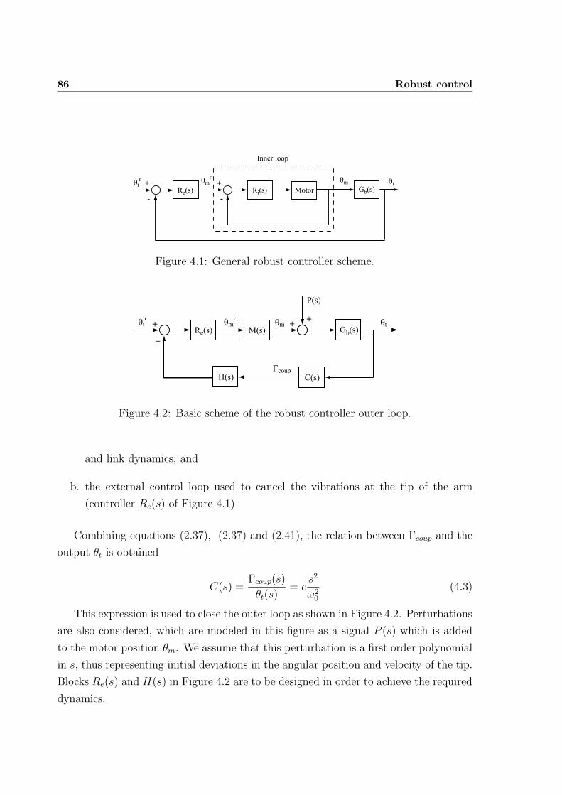
86 Robust control
Re(s) Ri(s) Motor Gb(s)θtr θm
rθm θt+
-
+
-
Inner loop
Figure 4.1: General robust controller scheme.
M(s)θtr
_
+ θmr
θm θt
Γcoup
Re(s)+
+
P(s)
Gb(s)
H(s) C(s)
Figure 4.2: Basic scheme of the robust controller outer loop.
and link dynamics; and
b. the external control loop used to cancel the vibrations at the tip of the arm
(controller Re(s) of Figure 4.1)
Combining equations (2.37), (2.37) and (2.41), the relation between Γcoup and the
output θt is obtained
C(s) =Γcoup(s)
θt(s)= c
s2
ω20
(4.3)
This expression is used to close the outer loop as shown in Figure 4.2. Perturbations
are also considered, which are modeled in this figure as a signal P (s) which is added
to the motor position θm. We assume that this perturbation is a first order polynomial
in s, thus representing initial deviations in the angular position and velocity of the tip.
Blocks Re(s) and H(s) in Figure 4.2 are to be designed in order to achieve the required
dynamics.
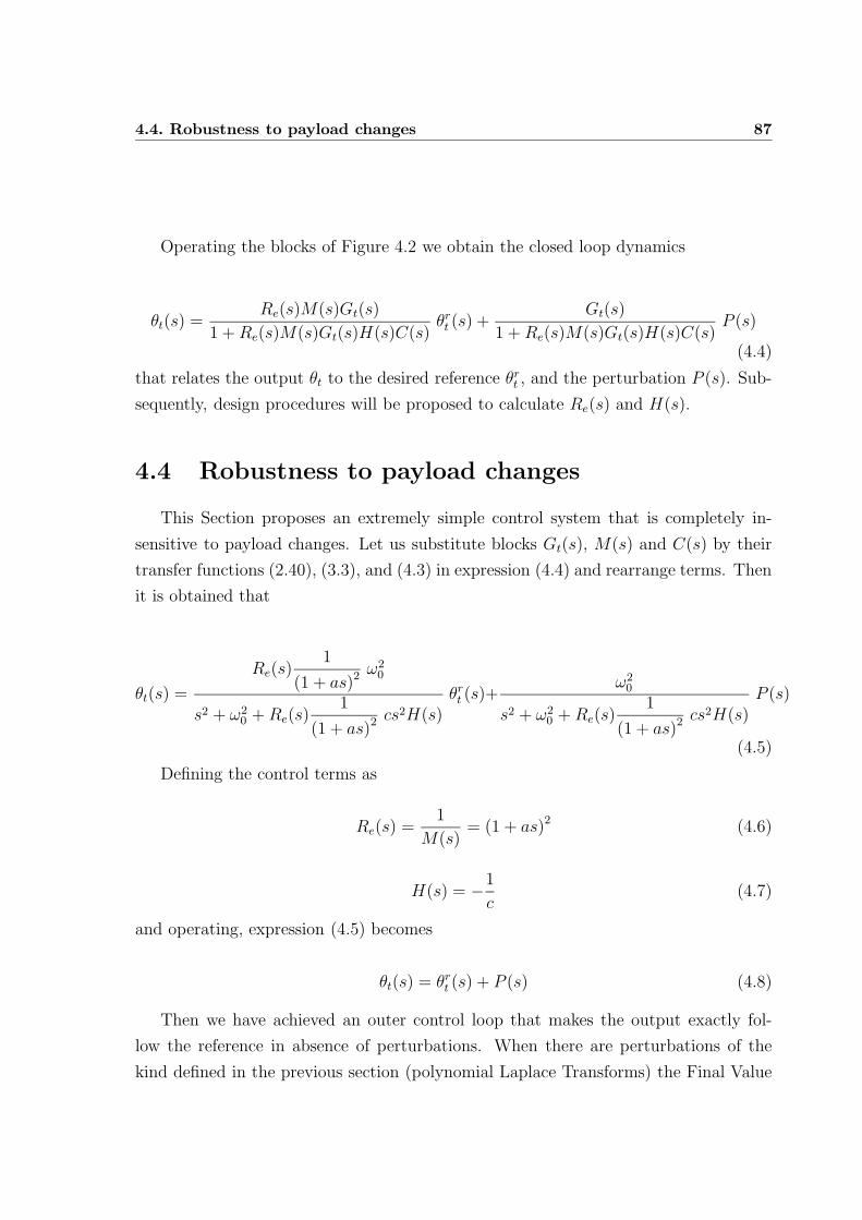
4.4. Robustness to payload changes 87
Operating the blocks of Figure 4.2 we obtain the closed loop dynamics
θt(s) =Re(s)M(s)Gt(s)
1 +Re(s)M(s)Gt(s)H(s)C(s)θrt (s) +
Gt(s)
1 +Re(s)M(s)Gt(s)H(s)C(s)P (s)
(4.4)
that relates the output θt to the desired reference θrt , and the perturbation P (s). Sub-
sequently, design procedures will be proposed to calculate Re(s) and H(s).
4.4 Robustness to payload changes
This Section proposes an extremely simple control system that is completely in-
sensitive to payload changes. Let us substitute blocks Gt(s), M(s) and C(s) by their
transfer functions (2.40), (3.3), and (4.3) in expression (4.4) and rearrange terms. Then
it is obtained that
θt(s) =
Re(s)1
(1 + as)2ω20
s2 + ω20 +Re(s)
1
(1 + as)2cs2H(s)
θrt (s)+ω20
s2 + ω20 +Re(s)
1
(1 + as)2cs2H(s)
P (s)
(4.5)
Defining the control terms as
Re(s) =1
M(s)= (1 + as)2 (4.6)
H(s) = −1
c(4.7)
and operating, expression (4.5) becomes
θt(s) = θrt (s) + P (s) (4.8)
Then we have achieved an outer control loop that makes the output exactly fol-
low the reference in absence of perturbations. When there are perturbations of the
kind defined in the previous section (polynomial Laplace Transforms) the Final Value
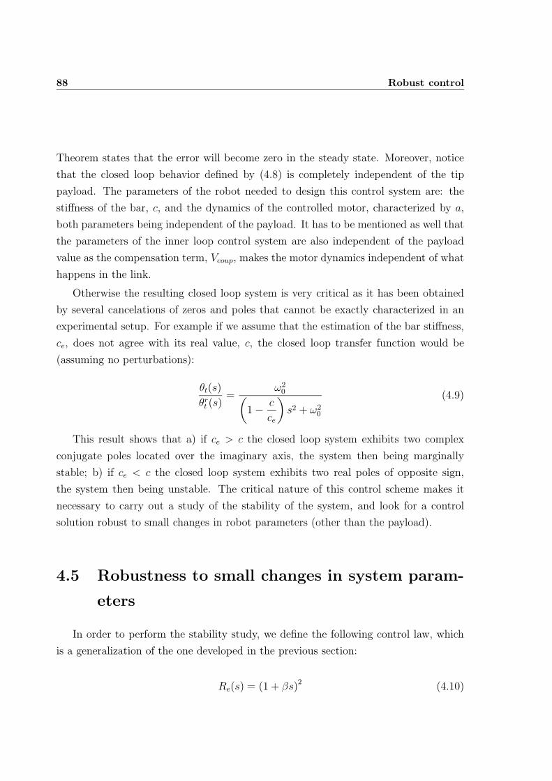
88 Robust control
Theorem states that the error will become zero in the steady state. Moreover, notice
that the closed loop behavior defined by (4.8) is completely independent of the tip
payload. The parameters of the robot needed to design this control system are: the
stiffness of the bar, c, and the dynamics of the controlled motor, characterized by a,
both parameters being independent of the payload. It has to be mentioned as well that
the parameters of the inner loop control system are also independent of the payload
value as the compensation term, Vcoup, makes the motor dynamics independent of what
happens in the link.
Otherwise the resulting closed loop system is very critical as it has been obtained
by several cancelations of zeros and poles that cannot be exactly characterized in an
experimental setup. For example if we assume that the estimation of the bar stiffness,
ce, does not agree with its real value, c, the closed loop transfer function would be
(assuming no perturbations):
θt(s)
θrt (s)=
ω20
(
1− c
ce
)
s2 + ω20
(4.9)
This result shows that a) if ce > c the closed loop system exhibits two complex
conjugate poles located over the imaginary axis, the system then being marginally
stable; b) if ce < c the closed loop system exhibits two real poles of opposite sign,
the system then being unstable. The critical nature of this control scheme makes it
necessary to carry out a study of the stability of the system, and look for a control
solution robust to small changes in robot parameters (other than the payload).
4.5 Robustness to small changes in system param-
eters
In order to perform the stability study, we define the following control law, which
is a generalization of the one developed in the previous section:
Re(s) = (1 + βs)2 (4.10)
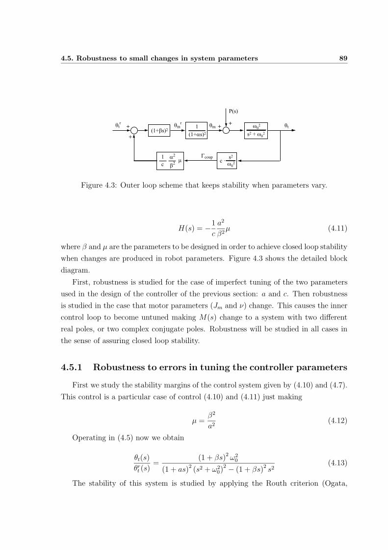
4.5. Robustness to small changes in system parameters 89
ω02
s2 + ω02
ω02
s2c ·
θtr
+
+ θmr
θm θt
Γcoup
++
P(s)
(1+βs)21
(1+αs)2
c
1 α2
β2µ
Figure 4.3: Outer loop scheme that keeps stability when parameters vary.
H(s) = −1
c
a2
β2µ (4.11)
where β and µ are the parameters to be designed in order to achieve closed loop stability
when changes are produced in robot parameters. Figure 4.3 shows the detailed block
diagram.
First, robustness is studied for the case of imperfect tuning of the two parameters
used in the design of the controller of the previous section: a and c. Then robustness
is studied in the case that motor parameters (Jm and ν) change. This causes the inner
control loop to become untuned making M(s) change to a system with two different
real poles, or two complex conjugate poles. Robustness will be studied in all cases in
the sense of assuring closed loop stability.
4.5.1 Robustness to errors in tuning the controller parameters
First we study the stability margins of the control system given by (4.10) and (4.7).
This control is a particular case of control (4.10) and (4.11) just making
µ =β2
a2(4.12)
Operating in (4.5) now we obtain
θt(s)
θrt (s)=
(1 + βs)2 ω20
(1 + as)2 (s2 + ω20)
2 − (1 + βs)2 s2(4.13)
The stability of this system is studied by applying the Routh criterion (Ogata,
90 Robust control
2001) to its characteristic polynomial:
Pc(s) =(a2 − β2
)s4 + 2 (a− β) s3 + a2ω2
0s2 + 2ω2
0as+ ω20 (4.14)
The obtained stability conditions are
a > 0 (4.15a)
−a < β <−a
ω20a
2 − 1(4.15b)
ω0a >√2 (4.15c)
which raise a serious problem. Section 4.4 proved that the proposed control works
correctly when the phase advance network is perfectly tuned with the motor dynamics
(β = a). Nevertheless condition (4.15b) states that β has to be of the opposite sign of
a in order to guarantee stability. In order to obtain good dynamic behavior robust to
payload changes, we can afford small deviations in the tuning of Re(s): β ≃ a, but not
a strong deviation as condition (4.15b) demands.
This fact justifies the inclusion of parameter µ as a new degree of freedom of the
control system. Controller H(s) in (4.11) also includes a normalization factor a2/β2.
If H(s) is of the form (4.11) the closed loop transfer function is
θt(s)
θrt (s)=
(1 + βs)2 ω20
(1 + as)2 (s2 + ω20)− (1 + βs)2 s2
a2
β2µ
(4.16)
and the characteristic polynomial is
P (s) = a2 (1− µ) s4 + 2a
(
1− µa
β
)
s3 +
(
1 + a2ω20 − µ
a2
β2
)
s2 + 2aω20s+ ω2
0 (4.17)
Routh criterion is applied again giving the following stability conditions:
1 > µ (4.18a)
4.5. Robustness to small changes in system parameters 91
β
a> µ (4.18b)
β2
a2+ β2ω2
0 > µ (4.18c)
a2ω20µ
(
1− a
β
)
+
(
1− µa
β
)(
1− µa2
β2
)
> 0 (4.18d)
(
β2ω20 +
β
a− µ
)(a
β
)2(
1− a
β
)
> 0 (4.18e)
which yield to
Case a < β. In this case conditions (4.18b), (4.18c) and (4.18d), are included
in (4.18a). Condition (4.18e) is also verified if (4.18a) is fulfilled, since it can be
simplified to
β2ω20 +
β
a> µ
In summary, in this case there is a single stability condition given by
µ ∈ (0, 1) (4.19)
Case a > β. In this other case, condition (4.18d) becomes
β2ω20 +
β
a< µ
which contradicts (4.18b). Then the closed loop system is always unstable in this case.
From this analysis we can conclude that choosing β ≥ a and µ as stated in (4.19)
makes the closed loop system stable. These two parameters can be tuned in such a way
that the system remains stable in the cases of: a) lack of precision in the knowledge of
parameter a, which describes the controlled motor dynamics; and b) lack of precision
in the estimation of parameter c. The cost to be paid is that closed loop dynamics
will become a bit worse than in (4.8), and we no longer get the perfect tracking of
92 Robust control
Section 4. But this ideal behavior can be approximated by choosing values of β close
to a and µ close to 1.
4.5.2 Robustness to changes of the motor parameters
Next the case in which motor parameters Jm and ν change will be considered.
Variation of these parameters produce changes in the inner loop transfer function in
the sense that now
M1(s) =1
(1 + a1s) (1 + a2s)(4.20)
where a1 and a2 are two different parameters that can be real or complex conjugate.
We mention that - in particular - friction coefficient ν often experiences large variations
through time.
The closed loop transfer function is now
θt(s)
θrt (s)=
(1 + βs)2 ω20
(1 + a1s) (1 + a2s) (s2 + ω20)
2 − (1 + βs)2 s2a2
β2µ
(4.21)
Application of the Routh criterion now leads to complicate stability conditions
that cannot be easily used for control design. Then we will use the Nyquist criterion in
order to derive sufficient conditions for stability. The characteristic equation of (4.21)
expressed in the frequency domain (s = jω) is
1 +ω2
ω20 − ω2
(1 + jβω)2
(1 + ja1ω) (1 + ja2ω)
a2
β2µ = 0 (4.22)
The resulting Nyquist plot is shown in Figure 4.4. This plot shows that the closed
loop system is stable if the following sufficient conditions are verified:
a. Denoting
L1(ω) =(1 + jβω)2
(1 + ja1ω) (1 + ja2ω), (4.23)
and ∠ the phase of a complex number:
∠L1(ω) ≥ 0, ∀ω. (4.24)
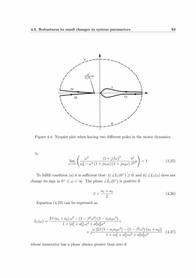
4.5. Robustness to small changes in system parameters 93
I
II
III
IV
V
VI
α2
α1α2µ
Figure 4.4: Nyquist plot when having two different poles in the motor dynamics.
b.
limω→∞
(
ω2
ω20 − ω2
(1 + jβω)2
(1 + ja1ω) (1 + ja2ω)
a2
β2µ
)
< 1 (4.25)
To fulfill condition (a) it is sufficient that: i) ∠L1(0+) ≥ 0; and ii) ∠L1(ω) does not
change its sign in 0+ ≤ ω < ∞. The phase ∠L1(0+) is positive if
β >a1 + a2
2(4.26)
Equation (4.23) can be expressed as
L1(ω) =2β (a1 + a2)ω
2 − (1− β2ω2) (1− a1a2ω2)
1 + (a21 + a22)ω2 + a21a
22ω
4+
+ jω [2β (1− a1a2ω
2)− (1− β2ω2) (a1 + a2)]
1 + (a21 + a22)ω2 + a21a
22ω
4(4.27)
whose numerator has a phase always greater than zero if
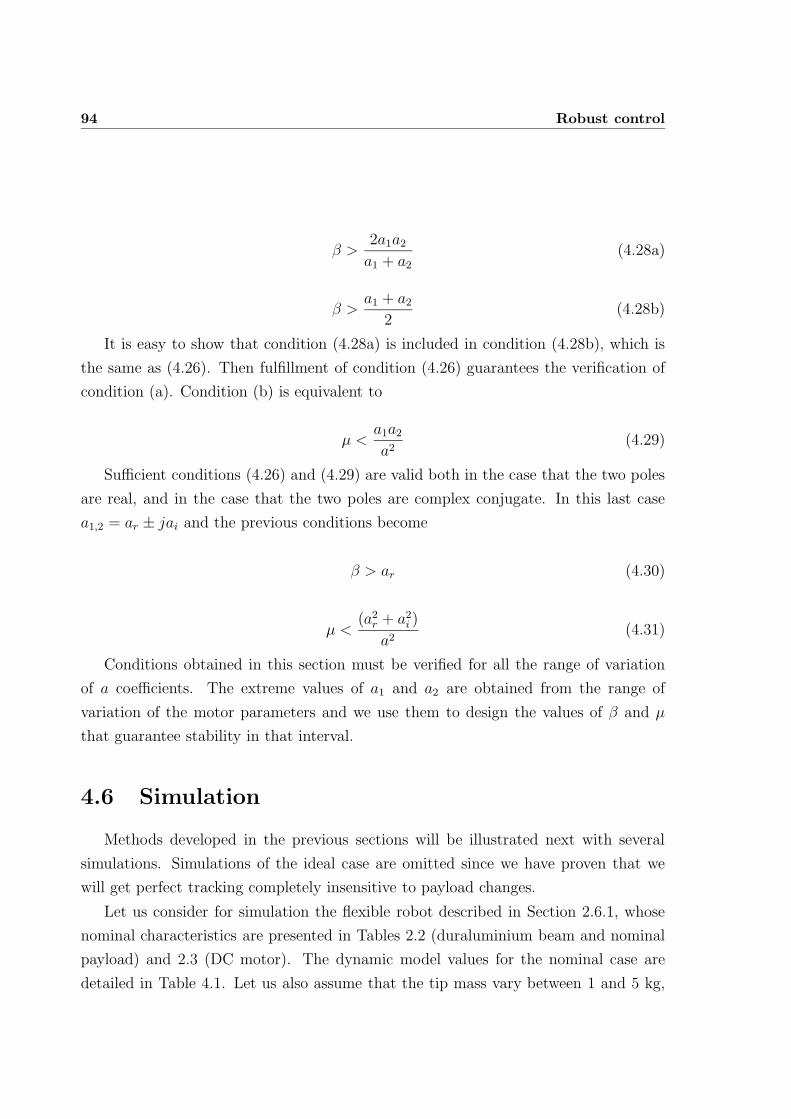
94 Robust control
β >2a1a2a1 + a2
(4.28a)
β >a1 + a2
2(4.28b)
It is easy to show that condition (4.28a) is included in condition (4.28b), which is
the same as (4.26). Then fulfillment of condition (4.26) guarantees the verification of
condition (a). Condition (b) is equivalent to
µ <a1a2a2
(4.29)
Sufficient conditions (4.26) and (4.29) are valid both in the case that the two poles
are real, and in the case that the two poles are complex conjugate. In this last case
a1,2 = ar ± jai and the previous conditions become
β > ar (4.30)
µ <(a2r + a2i )
a2(4.31)
Conditions obtained in this section must be verified for all the range of variation
of a coefficients. The extreme values of a1 and a2 are obtained from the range of
variation of the motor parameters and we use them to design the values of β and µ
that guarantee stability in that interval.
4.6 Simulation
Methods developed in the previous sections will be illustrated next with several
simulations. Simulations of the ideal case are omitted since we have proven that we
will get perfect tracking completely insensitive to payload changes.
Let us consider for simulation the flexible robot described in Section 2.6.1, whose
nominal characteristics are presented in Tables 2.2 (duraluminium beam and nominal
payload) and 2.3 (DC motor). The dynamic model values for the nominal case are
detailed in Table 4.1. Let us also assume that the tip mass vary between 1 and 5 kg,
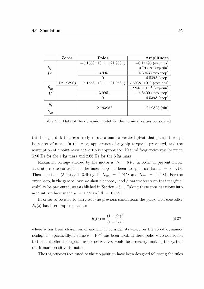
4.6. Simulation 95
Zeros Poles Amplitudes
θtV
−5.1568 · 10−3 ± 21.9681j −0.14496 (exp·cos)−0.79919 (exp·sin)
−3.9951 −4.3943 (exp·step)0 4.5393 (step)
θmV
±21.9398j −5.1568 · 10−3 ± 21.9681j 7.5038 · 10−4 (exp·cos)1.9948 · 10−3 (exp·sin)
−3.9951 −4.5400 (exp·step)0 4.5393 (step)
θtθm
±21.9398j 21.9398 (sin)
Table 4.1: Data of the dynamic model for the nominal values considered
this being a disk that can freely rotate around a vertical pivot that passes through
its center of mass. In this case, appearance of any tip torque is prevented, and the
assumption of a point mass at the tip is appropriate. Natural frequencies vary between
5.96 Hz for the 1 kg mass and 2.66 Hz for the 5 kg mass.
Maximum voltage allowed by the motor is VM = 6 V . In order to prevent motor
saturations the controller of the inner loop has been designed so that a = 0.0278.
Then equations (3.4a) and (3.4b) yield Kpm = 0.9158 and Kvm = 0.0481. For the
outer loop, in the general case we should choose µ and β parameters such that marginal
stability be prevented, as established in Section 4.5.1. Taking these considerations into
account, we have made µ = 0.99 and β = 0.029.
In order to be able to carry out the previous simulations the phase lead controller
Re(s) has been implemented as
Re(s) =(1 + βs)2
(1 + δs)2(4.32)
where δ has been chosen small enough to consider its effect on the robot dynamics
negligible. Specifically, a value δ = 10−4 has been used. If these poles were not added
to the controller the explicit use of derivatives would be necessary, making the system
much more sensitive to noise.
The trajectories requested to the tip position have been designed following the rules
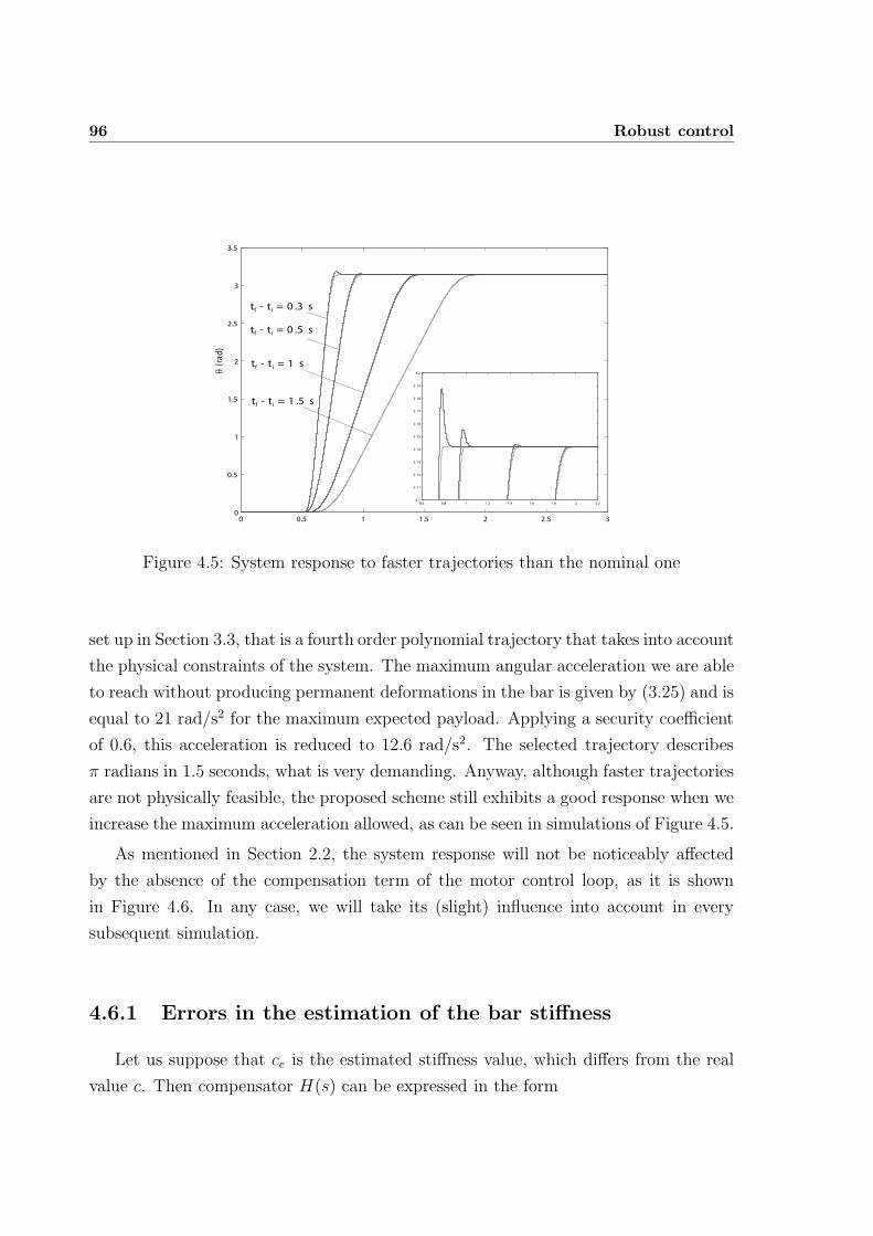
96 Robust control
0 0.5 1 1.5 2 2.5 30
0.5
1
1.5
2
2.5
3
3.5
tf - t i = 0 .3 s
tf - t i = 0 .5 s
tf - t i = 1 s
tf - t i = 1 .5 s
0.6 0.8 1 1.2 1.4 1.6 1.8 2 2.23.1
3.11
3.12
3.13
3.14
3.15
3.16
3.17
3.18
3.19
3.2θ(r
ad
)
Figure 4.5: System response to faster trajectories than the nominal one
set up in Section 3.3, that is a fourth order polynomial trajectory that takes into account
the physical constraints of the system. The maximum angular acceleration we are able
to reach without producing permanent deformations in the bar is given by (3.25) and is
equal to 21 rad/s2 for the maximum expected payload. Applying a security coefficient
of 0.6, this acceleration is reduced to 12.6 rad/s2. The selected trajectory describes
π radians in 1.5 seconds, what is very demanding. Anyway, although faster trajectories
are not physically feasible, the proposed scheme still exhibits a good response when we
increase the maximum acceleration allowed, as can be seen in simulations of Figure 4.5.
As mentioned in Section 2.2, the system response will not be noticeably affected
by the absence of the compensation term of the motor control loop, as it is shown
in Figure 4.6. In any case, we will take its (slight) influence into account in every
subsequent simulation.
4.6.1 Errors in the estimation of the bar stiffness
Let us suppose that ce is the estimated stiffness value, which differs from the real
value c. Then compensator H(s) can be expressed in the form
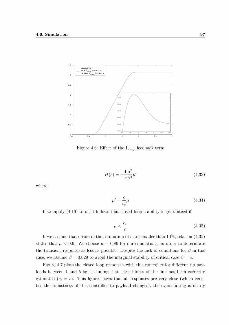
4.6. Simulation 97
0 0.5 1 1.5 2 2.5 30
0.5
1
1.5
2
2.5
3
3.5
referencewith Γ
coupfeedback
without Γcoup
feedback
1.92 1.94 1.96 1.98 2 2.02 2.04
3.1415
3.1416
3.1417
3.1418
3.1419
3.142
Figure 4.6: Effect of the Γcoup feedback term
H(s) = −1
c
α2
β2µ′ (4.33)
where
µ′ =c
ceµ (4.34)
If we apply (4.19) to µ′, it follows that closed loop stability is guaranteed if
µ <cec
(4.35)
If we assume that errors in the estimation of c are smaller than 10%, relation (4.35)
states that µ < 0.9. We choose µ = 0.89 for our simulations, in order to deteriorate
the transient response as less as possible. Despite the lack of conditions for β in this
case, we assume β = 0.029 to avoid the marginal stability of critical case β = a.
Figure 4.7 plots the closed loop responses with this controller for different tip pay-
loads between 1 and 5 kg, assuming that the stiffness of the link has been correctly
estimated (ce = c). This figure shows that all responses are very close (which certi-
fies the robustness of this controller to payload changes), the overshooting is nearly
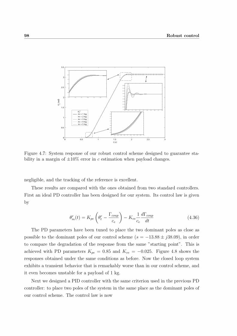
98 Robust control
0 0.5 1 1.5 2 2.5 30
0.5
1
1.5
2
2.5
3
3.5
θrt
m = 1 kg
m = 2 kg
m = 3 kg
m = 4 kg
m = 5 kg
0.6 0.62 0.64 0.66 0.68 0.7 0.72 0.74 0.76 0.78 0.80
0.02
0.04
0.06
0.08
0.1
0.12
0.14
0.16
0.18
0.2
1.7 1.75 1.8 1.85 1.9 1.95 22.9
2.95
3
3.05
3.1
3.15
3.2
1.8 1.9 2 2.1 2.2 2.3 2.4 2.5 2.6 2.7 2.83.13
3.132
3.134
3.136
3.138
3.14
3.142
3.144
3.146
3.148
t (s )
θt
(ra
d)
Figure 4.7: System response of our robust control scheme designed to guarantee sta-bility in a margin of ±10% error in c estimation when payload changes.
negligible, and the tracking of the reference is excellent.
These results are compared with the ones obtained from two standard controllers.
First an ideal PD controller has been designed for our system. Its control law is given
by
θrm(t) = Kpe
(
θrt −Γcoup
ce
)
−Kve
1
ce
dΓcoup
dt(4.36)
The PD parameters have been tuned to place the two dominant poles as close as
possible to the dominant poles of our control scheme (s = −13.88 ± j38.09), in order
to compare the degradation of the response from the same ”starting point”. This is
achieved with PD parameters Kpe = 0.85 and Kve = −0.025. Figure 4.8 shows the
responses obtained under the same conditions as before. Now the closed loop system
exhibits a transient behavior that is remarkably worse than in our control scheme, and
it even becomes unstable for a payload of 1 kg.
Next we designed a PID controller with the same criterion used in the previous PD
controller: to place two poles of the system in the same place as the dominant poles of
our control scheme. The control law is now
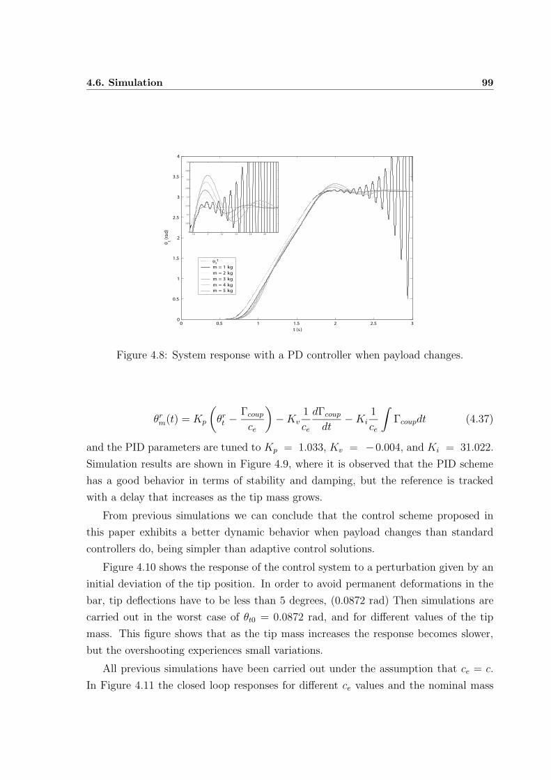
4.6. Simulation 99
0 0.5 1 1.5 2 2.5 30
0.5
1
1.5
2
2.5
3
3.5
4
1.8 2 2.2 2.4 2.6 2.83
3.05
3.1
3.15
3.2
3.25
3.3
3.35
3.4
t (s )
θt
(ra
d)
θrt
m = 1 kg
m = 2 kg
m = 3 kg
m = 4 kg
m = 5 kg
Figure 4.8: System response with a PD controller when payload changes.
θrm(t) = Kp
(
θrt −Γcoup
ce
)
−Kv
1
ce
dΓcoup
dt−Ki
1
ce
∫
Γcoupdt (4.37)
and the PID parameters are tuned to Kp = 1.033, Kv = −0.004, and Ki = 31.022.
Simulation results are shown in Figure 4.9, where it is observed that the PID scheme
has a good behavior in terms of stability and damping, but the reference is tracked
with a delay that increases as the tip mass grows.
From previous simulations we can conclude that the control scheme proposed in
this paper exhibits a better dynamic behavior when payload changes than standard
controllers do, being simpler than adaptive control solutions.
Figure 4.10 shows the response of the control system to a perturbation given by an
initial deviation of the tip position. In order to avoid permanent deformations in the
bar, tip deflections have to be less than 5 degrees, (0.0872 rad) Then simulations are
carried out in the worst case of θt0 = 0.0872 rad, and for different values of the tip
mass. This figure shows that as the tip mass increases the response becomes slower,
but the overshooting experiences small variations.
All previous simulations have been carried out under the assumption that ce = c.
In Figure 4.11 the closed loop responses for different ce values and the nominal mass
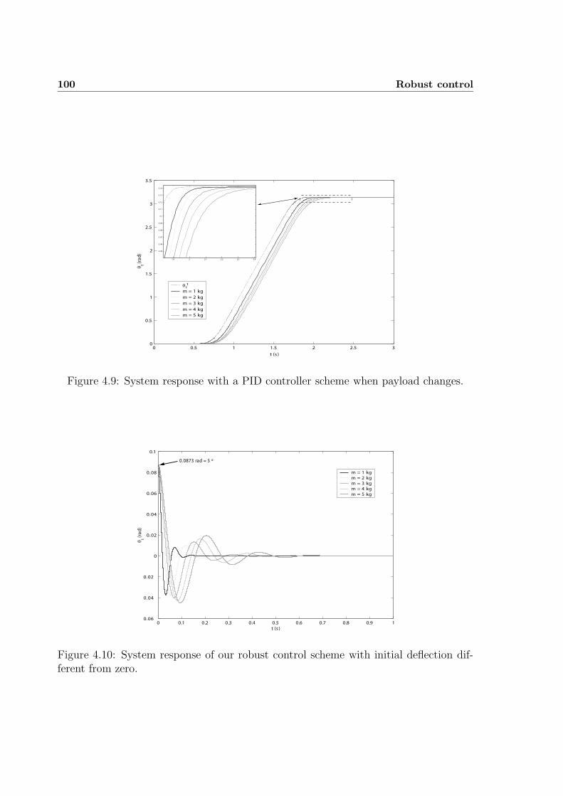
100 Robust control
0 0.5 1 1.5 2 2.5 30
0.5
1
1.5
2
2.5
3
3.5
1.9 2 2.1 2.2 2.3 2.4
3.05
3.06
3.07
3.08
3.09
3.1
3.11
3.12
3.13
3.14
t (s )
θt
(ra
d)
θrt
m = 1 kg
m = 2 kg
m = 3 kg
m = 4 kg
m = 5 kg
Figure 4.9: System response with a PID controller scheme when payload changes.
0 0.1 0.2 0.3 0.4 0.5 0.6 0.7 0.8 0.9 10.06
0.04
0.02
0
0.02
0.04
0.06
0.08
0.1
t (s )
θt
(ra
d)
m = 1 kg
m = 2 kg
m = 3 kg
m = 4 kg
m = 5 kg
0.0873 rad = 5 º
Figure 4.10: System response of our robust control scheme with initial deflection dif-ferent from zero.
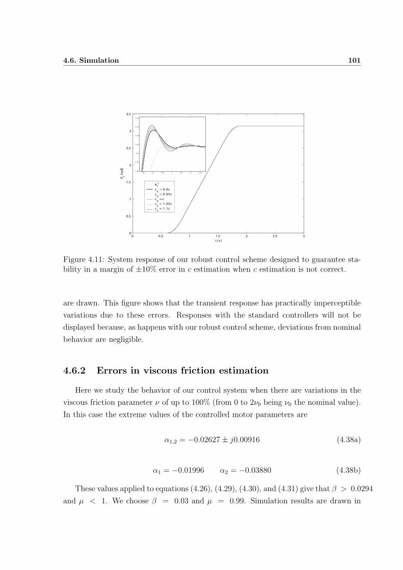
4.6. Simulation 101
0 0.5 1 1.5 2 2.5 30
0.5
1
1.5
2
2.5
3
3.5
θrt
ce
= 0.9c
ce
= 0.95c
ce
= c
ce
= 1.05c
ce
= 1.1c
1.85 1.9 1.95 2 2.05 2.1 2.15
3.136
3.138
3.14
3.142
3.144
3.146
3.148
t (s )
θt
(ra
d)
Figure 4.11: System response of our robust control scheme designed to guarantee sta-bility in a margin of ±10% error in c estimation when c estimation is not correct.
are drawn. This figure shows that the transient response has practically imperceptible
variations due to these errors. Responses with the standard controllers will not be
displayed because, as happens with our robust control scheme, deviations from nominal
behavior are negligible.
4.6.2 Errors in viscous friction estimation
Here we study the behavior of our control system when there are variations in the
viscous friction parameter ν of up to 100% (from 0 to 2ν0 being ν0 the nominal value).
In this case the extreme values of the controlled motor parameters are
α1,2 = −0.02627± j0.00916 (4.38a)
α1 = −0.01996 α2 = −0.03880 (4.38b)
These values applied to equations (4.26), (4.29), (4.30), and (4.31) give that β > 0.0294
and µ < 1. We choose β = 0.03 and µ = 0.99. Simulation results are drawn in
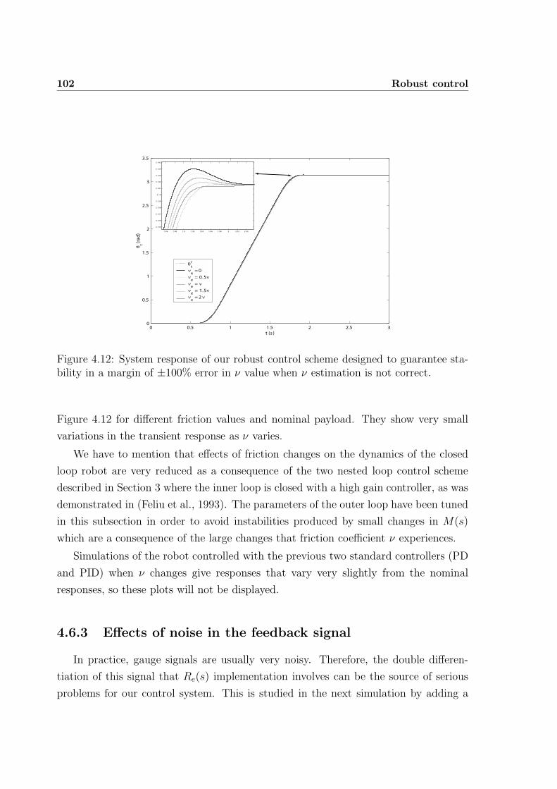
102 Robust control
0 0.5 1 1.5 2 2.5 30
0.5
1
1.5
2
2.5
3
3.5
t (s )
θt
(ra
d)
θt
r
νe
= 0
νe
= 0.5ν
νe
= ν
νe
= 1.5ν
νe
= 2 ν
1.86 1.88 1.9 1.92 1.94 1.96 1.98 2 2.02 2.04
3.135
3.136
3.137
3.138
3.139
3.14
3.141
3.142
3.143
3.144
3.145
Figure 4.12: System response of our robust control scheme designed to guarantee sta-bility in a margin of ±100% error in ν value when ν estimation is not correct.
Figure 4.12 for different friction values and nominal payload. They show very small
variations in the transient response as ν varies.
We have to mention that effects of friction changes on the dynamics of the closed
loop robot are very reduced as a consequence of the two nested loop control scheme
described in Section 3 where the inner loop is closed with a high gain controller, as was
demonstrated in (Feliu et al., 1993). The parameters of the outer loop have been tuned
in this subsection in order to avoid instabilities produced by small changes in M(s)
which are a consequence of the large changes that friction coefficient ν experiences.
Simulations of the robot controlled with the previous two standard controllers (PD
and PID) when ν changes give responses that vary very slightly from the nominal
responses, so these plots will not be displayed.
4.6.3 Effects of noise in the feedback signal
In practice, gauge signals are usually very noisy. Therefore, the double differen-
tiation of this signal that Re(s) implementation involves can be the source of serious
problems for our control system. This is studied in the next simulation by adding a
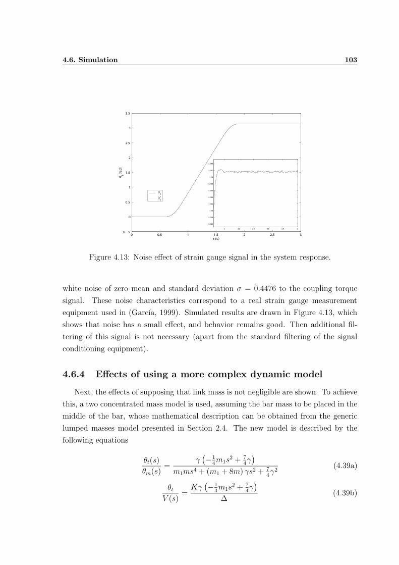
4.6. Simulation 103
0 0.5 1 1.5 2 2.5 30. 5
0
0.5
1
1.5
2
2.5
3
3.5
t (s )
θt
(ra
d)
θt
θt
r
2 2.2 2.4 2.6 2.8 3
3.126
3.128
3.13
3.132
3.134
3.136
3.138
3.14
3.142
3.144
Figure 4.13: Noise effect of strain gauge signal in the system response.
white noise of zero mean and standard deviation σ = 0.4476 to the coupling torque
signal. These noise characteristics correspond to a real strain gauge measurement
equipment used in (Garcıa, 1999). Simulated results are drawn in Figure 4.13, which
shows that noise has a small effect, and behavior remains good. Then additional fil-
tering of this signal is not necessary (apart from the standard filtering of the signal
conditioning equipment).
4.6.4 Effects of using a more complex dynamic model
Next, the effects of supposing that link mass is not negligible are shown. To achieve
this, a two concentrated mass model is used, assuming the bar mass to be placed in the
middle of the bar, whose mathematical description can be obtained from the generic
lumped masses model presented in Section 2.4. The new model is described by the
following equations
θt(s)
θm(s)=
γ(−1
4m1s
2 + 74γ)
m1ms4 + (m1 + 8m) γs2 + 74γ2
(4.39a)
θtV (s)
=Kγ
(−1
4m1s
2 + 74γ)
∆(4.39b)
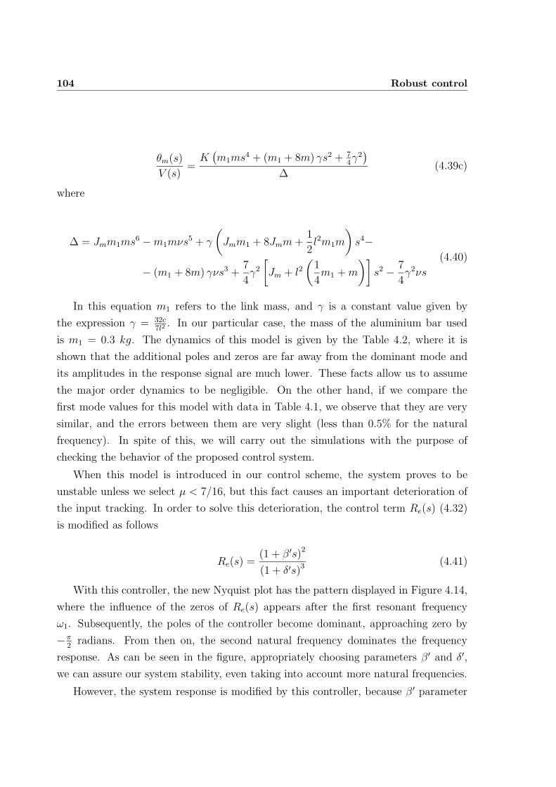
104 Robust control
θm(s)
V (s)=
K(m1ms4 + (m1 + 8m) γs2 + 7
4γ2)
∆(4.39c)
where
∆ = Jmm1ms6 −m1mνs5 + γ
(
Jmm1 + 8Jmm+1
2l2m1m
)
s4−
− (m1 + 8m) γνs3 +7
4γ2
[
Jm + l2(1
4m1 +m
)]
s2 − 7
4γ2νs
(4.40)
In this equation m1 refers to the link mass, and γ is a constant value given by
the expression γ = 32c7l2
. In our particular case, the mass of the aluminium bar used
is m1 = 0.3 kg. The dynamics of this model is given by the Table 4.2, where it is
shown that the additional poles and zeros are far away from the dominant mode and
its amplitudes in the response signal are much lower. These facts allow us to assume
the major order dynamics to be negligible. On the other hand, if we compare the
first mode values for this model with data in Table 4.1, we observe that they are very
similar, and the errors between them are very slight (less than 0.5% for the natural
frequency). In spite of this, we will carry out the simulations with the purpose of
checking the behavior of the proposed control system.
When this model is introduced in our control scheme, the system proves to be
unstable unless we select µ < 7/16, but this fact causes an important deterioration of
the input tracking. In order to solve this deterioration, the control term Re(s) (4.32)
is modified as follows
Re(s) =(1 + β ′s)2
(1 + δ′s)3(4.41)
With this controller, the new Nyquist plot has the pattern displayed in Figure 4.14,
where the influence of the zeros of Re(s) appears after the first resonant frequency
ω1. Subsequently, the poles of the controller become dominant, approaching zero by
−π2radians. From then on, the second natural frequency dominates the frequency
response. As can be seen in the figure, appropriately choosing parameters β ′ and δ′,
we can assure our system stability, even taking into account more natural frequencies.
However, the system response is modified by this controller, because β ′ parameter
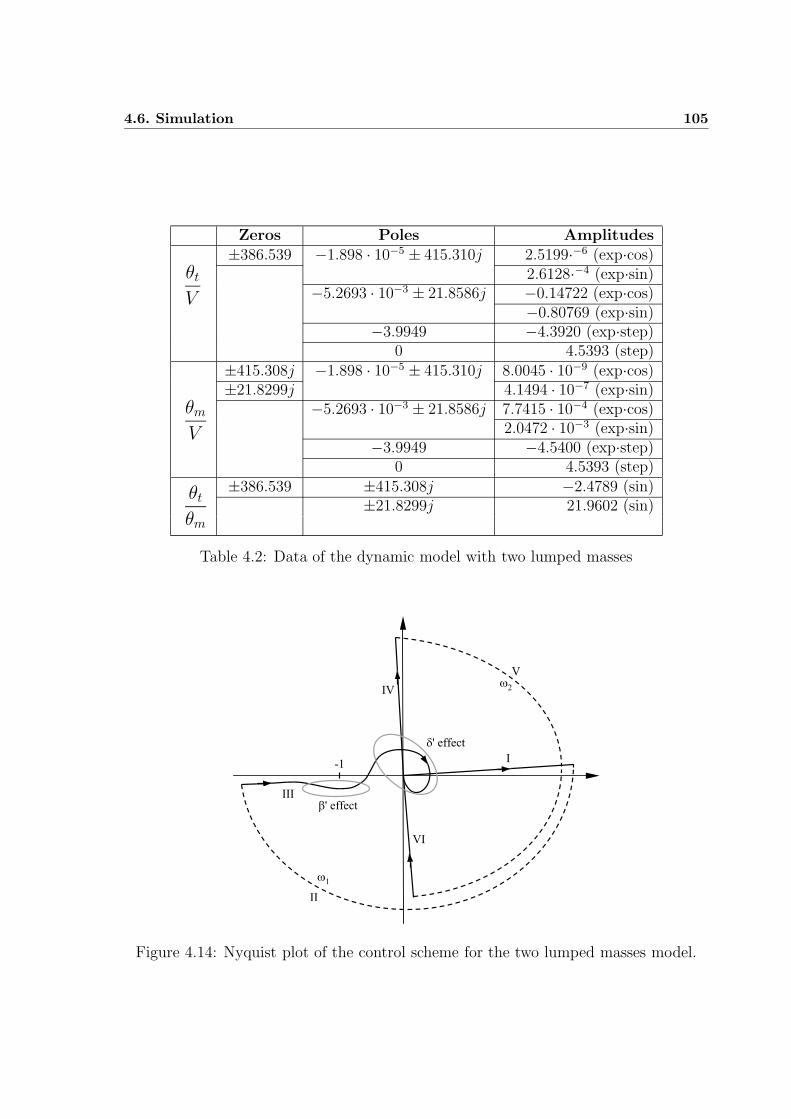
4.6. Simulation 105
Zeros Poles Amplitudes
θtV
±386.539 −1.898 · 10−5 ± 415.310j 2.5199·−6 (exp·cos)2.6128·−4 (exp·sin)
−5.2693 · 10−3 ± 21.8586j −0.14722 (exp·cos)−0.80769 (exp·sin)
−3.9949 −4.3920 (exp·step)0 4.5393 (step)
θmV
±415.308j −1.898 · 10−5 ± 415.310j 8.0045 · 10−9 (exp·cos)±21.8299j 4.1494 · 10−7 (exp·sin)
−5.2693 · 10−3 ± 21.8586j 7.7415 · 10−4 (exp·cos)2.0472 · 10−3 (exp·sin)
−3.9949 −4.5400 (exp·step)0 4.5393 (step)
θtθm
±386.539 ±415.308j −2.4789 (sin)±21.8299j 21.9602 (sin)
Table 4.2: Data of the dynamic model with two lumped masses
II
I
III
IV
V
VI
β' effect
δ' effect
-1
ω1
ω2
Figure 4.14: Nyquist plot of the control scheme for the two lumped masses model.
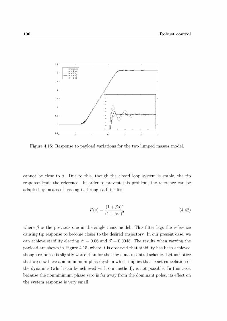
106 Robust control
00.5
0
0.5
1
1.5
2
2.5
3
3.5
referencem = 2 kgm = 3 kgm = 4 kgm = 5 kg
0.5 1 1.5 2 2.5 3
1.8 2 2.2 2.4 2.6 2.83.1
3.11
3.12
3.13
3.14
3.15
3.16
3.17
3.18
3.19
3.2
Figure 4.15: Response to payload variations for the two lumped masses model.
cannot be close to a. Due to this, though the closed loop system is stable, the tip
response leads the reference. In order to prevent this problem, the reference can be
adapted by means of passing it through a filter like
F (s) =(1 + βs)2
(1 + β ′s)2(4.42)
where β is the previous one in the single mass model. This filter lags the reference
causing tip response to become closer to the desired trajectory. In our present case, we
can achieve stability electing β ′ = 0.06 and δ′ = 0.0048. The results when varying the
payload are shown in Figure 4.15, where it is observed that stability has been achieved
though response is slightly worse than for the single mass control scheme. Let us notice
that we now have a nonminimum phase system which implies that exact cancelation of
the dynamics (which can be achieved with our method), is not possible. In this case,
because the nonminimum phase zero is far away from the dominant poles, its effect on
the system response is very small.
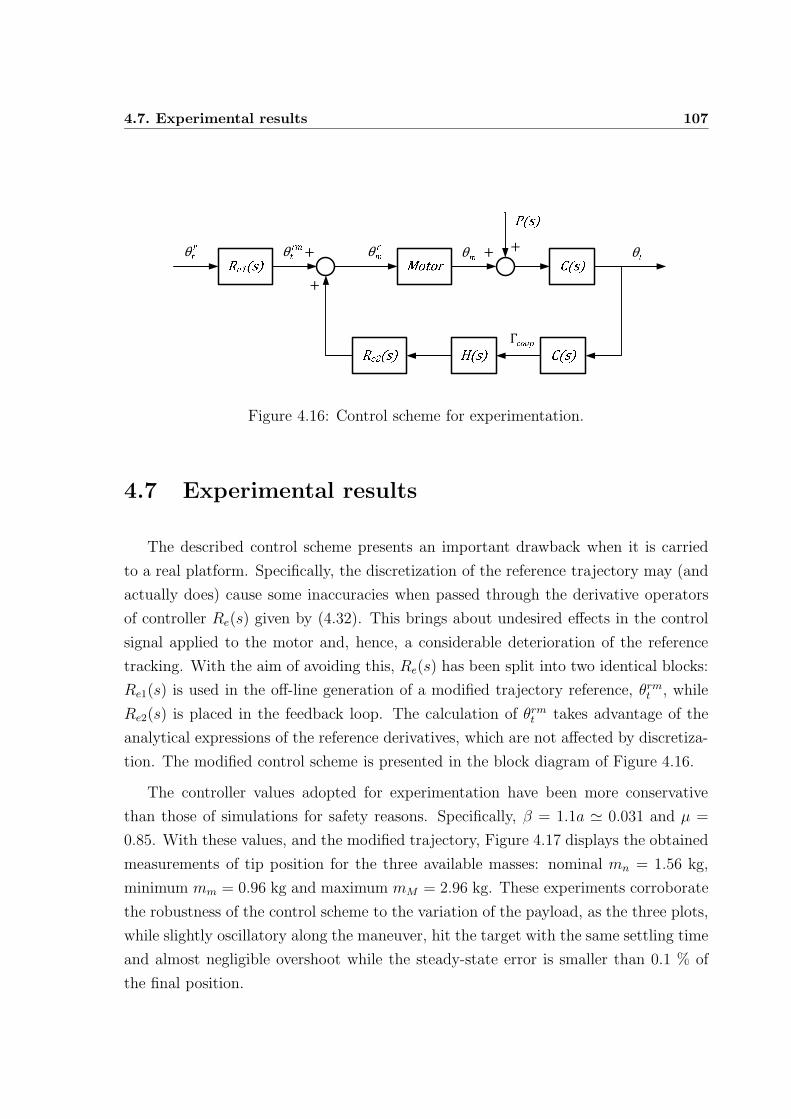
4.7. Experimental results 107
Figure 4.16: Control scheme for experimentation.
4.7 Experimental results
The described control scheme presents an important drawback when it is carried
to a real platform. Specifically, the discretization of the reference trajectory may (and
actually does) cause some inaccuracies when passed through the derivative operators
of controller Re(s) given by (4.32). This brings about undesired effects in the control
signal applied to the motor and, hence, a considerable deterioration of the reference
tracking. With the aim of avoiding this, Re(s) has been split into two identical blocks:
Re1(s) is used in the off-line generation of a modified trajectory reference, θrmt , while
Re2(s) is placed in the feedback loop. The calculation of θrmt takes advantage of the
analytical expressions of the reference derivatives, which are not affected by discretiza-
tion. The modified control scheme is presented in the block diagram of Figure 4.16.
The controller values adopted for experimentation have been more conservative
than those of simulations for safety reasons. Specifically, β = 1.1a ≃ 0.031 and µ =
0.85. With these values, and the modified trajectory, Figure 4.17 displays the obtained
measurements of tip position for the three available masses: nominal mn = 1.56 kg,
minimum mm = 0.96 kg and maximum mM = 2.96 kg. These experiments corroborate
the robustness of the control scheme to the variation of the payload, as the three plots,
while slightly oscillatory along the maneuver, hit the target with the same settling time
and almost negligible overshoot while the steady-state error is smaller than 0.1 % of
the final position.
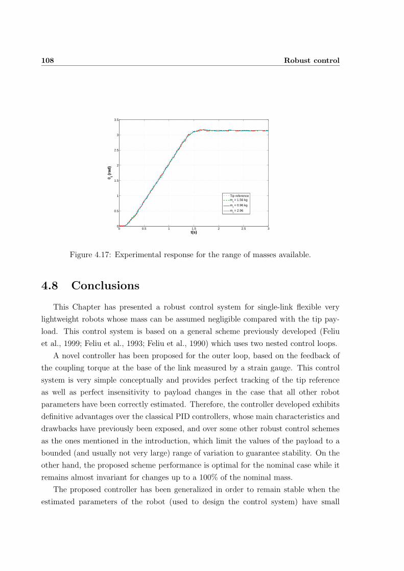
108 Robust control
0 0.5 1 1.5 2 2.5 30
0.5
1
1.5
2
2.5
3
3.5
t(s)
θ t (ra
d)
Tip referencem
t = 1.56 kg
mt = 0.96 kg
mt = 2.96
Figure 4.17: Experimental response for the range of masses available.
4.8 Conclusions
This Chapter has presented a robust control system for single-link flexible very
lightweight robots whose mass can be assumed negligible compared with the tip pay-
load. This control system is based on a general scheme previously developed (Feliu
et al., 1999; Feliu et al., 1993; Feliu et al., 1990) which uses two nested control loops.
A novel controller has been proposed for the outer loop, based on the feedback of
the coupling torque at the base of the link measured by a strain gauge. This control
system is very simple conceptually and provides perfect tracking of the tip reference
as well as perfect insensitivity to payload changes in the case that all other robot
parameters have been correctly estimated. Therefore, the controller developed exhibits
definitive advantages over the classical PID controllers, whose main characteristics and
drawbacks have previously been exposed, and over some other robust control schemes
as the ones mentioned in the introduction, which limit the values of the payload to a
bounded (and usually not very large) range of variation to guarantee stability. On the
other hand, the proposed scheme performance is optimal for the nominal case while it
remains almost invariant for changes up to a 100% of the nominal mass.
The proposed controller has been generalized in order to remain stable when the
estimated parameters of the robot (used to design the control system) have small
4.8. Conclusions 109
errors, or vary through time. Simulations of this control system prove the correctness
of the theoretical results, showing that this new controller remains almost insensitive to
payload changes and performs an excellent tracking of the reference, while exhibiting
quite a robust behavior to changes in the link parameters, motor parameters, and
measurement noises.
Finally, after a final consideration on the modification of the trajectory for practical
purposes, some experiments have been carried out and the excellent performance of
the control strategy has been verified.

110 Robust control
Chapter 5
Adaptive control
5.1 Introduction
Taking up again arguments commented in the previous Chapter, the controllers
developed for regulation of robotic systems must be, as insensitive as possible to changes
or uncertainties in the system parameters, as they might (or even must) change along
operation. This has been achieved by means of the robust controller presented there.
That control strategy reacts automatically to any change in the dynamics to carry
out the desired trajectory. This property has two sides. The bright side is that we man-
age to perform the maneuver under any (or, at least, a wide range of) circumstances or
system parameters. However, this robust controller is completely “blind” in the sense
that it demands as much control effort as it needs without having into account the
physical limits of the actuator, and the control scheme neither modifies the controller
nor the maneuver when the system is not operating under nominal conditions. This
might lead to the saturation of the actuator, and the consequent malfunction of the
system. In order to deal with these issues, we need more information from the sys-
tem. This can be obtained using a more complete sensorial system or some estimation
techniques that, with the actual sensors, provide that information.
This Chapter presents an adaptive control approach, also mentioned in the in-
troduction of previous Chapter, that takes advantage of a new, simple identification
technique based on the sensorial system proposed in the previous Chapter. A few smart
calculations identify the actual value of the payload (as it is the most frequently varied
112 Adaptive control
parameter of a robot) in a very short time, making it possible to tune the controller
depending on these values. The controller selection is based on attaining the same
specifications as would be used for the nominal values. A number of simulations have
been carried out regarding the estimation process and the adaptive controller, and
some experiments performed corroborate with the good results obtained numerically.
5.2 Previous experiences in adaptive control of flex-
ible systems
Adaptive control is a nonlinear control strategy that varies the values of the con-
troller parameters, depending on some criteria based upon the data collected from
the previous movements, to achieve an optimal performance even when the changes in
the plant are significant. A classification of the different adaptive schemes is detailed
in (Astrom and Wittenmark, 1995), where four types are described: gain scheduling,
which adjusts controller parameters on the basis of the operating conditions which
change during the process; model-reference adaptive systems (MRAS) which compare
the actual system output and the model output and modify the controller so that the
error between them is small; self-tuning regulators (STR), which update the system
parameters from the estimation process and obtain the controller constants from the
solution of a design problem using the estimated parameters; and dual control schemes,
where nonlinear stochastic control theory is used for achieving the abstract problem
formulation.
In his survey on flexible robots (Book, 1993), Prof. Book already predicted that this
field of control would contribute significatively to the, by then, open topics in flexible
robotics. Indeed, a major effort has been devoted in literature to the development of
adaptive control schemes for controlling flexible robots, usually based on a two-stage
process in which the adaptation of the controller is preceded by a system identification
stage (Rovner and Cannon, 1987; Koivo and Lee, 1989). Some of these controllers
need to recalculate the whole model, e.g. the MRAS proposed in (Siciliano et al.,
1986) for a single-link flexible arm, or the passivity-based control approach of the
MRAS presented in (Damaren, 1996; Christoforou and Damaren, 2000) for the multi-
link case. (Damaren, 1996) presents a numerical example based on a model of the
5.2. Previous experiences in adaptive control of flexible systems 113
Shuttle Remote Manipulator System (SRMS), where all the payload mass properties
are identified, while (Christoforou and Damaren, 2000) the previous adaptive scheme
is extended with an identification stage that also determines the arm mass properties
and presents experimental results on a planar 3-link flexible manipulator. However,
this solution may become considerably inefficient, as most of the parameters do not
change its value for long periods of time, and other authors have proposed different
STRs, focusing this identification stage in a specific, representative parameter of the
system, which serves to redesign the set of controller constants to keep the desired
system specifications. Lately, a new current of adaptive control involving intelligent
techniques such as the neural networks and/or sliding control has emerged. An example
can be found in (Tian and Collins, 2004), where a fuzzy logic controller is used to
update the parameters of a dynamic recurrent neural network which approximates the
inverse dynamics of the robotic manipulator. However, adaptiveness is not limited
to aforementioned schemes, but can be applied to any control strategy that makes
use of a controller with some adjustable parameters (that is, any sort of control). In
previous literature, adaptive schemes have been built upon the base of the most diverse
controllers, e.g. energy-based (Lee et al., 2001) or command shapers (Rhim and Book,
2004), with the benefits and drawbacks of these, but with an improvement in the
performance under uncertainties.
Obviously, an adaptive scheme is as good as its identification stage is. And good-
ness can be measured in terms of estimation time. Hence, those controllers based on
fuzzy logic or neural networks, which are usually slower, operate more time under un-
certainty, losing performance along the way. In (Feliu et al., 1999), the identification
process focuses in identifying the payload which, as aforementioned, is the most variable
parameter in the usual operation of a robotic arm. The proposed estimator is based on
the measurements from an accelerometer placed at the payload and the control signal.
That work has, however, some inaccuracies because it includes the motor dynamics in
the estimation process, which involves the parameters of the motor, rotor inertia and
viscous friction, and the Coulomb friction. While the rotor inertia remains unchanged,
the viscous friction is strongly dependant with temperature, and varies even along a
single maneuver. On the other hand, the Coulomb friction inserts a strong nonlinearity
in the identification process which is difficult to pre-compensate accurately and may
114 Adaptive control
cause an inexact estimation. A different approach is taken by (Trapero et al., 2007)
for the identification stage. They propose a frequency estimator based on an algebraic
method which has the drawback that it can only be applied to sinusoid-like signals,
and hence, it can only be applied to the identification of the system frequencies while
the robot actuator is stopped and the link is vibrating steadily.
In the present Chapter, a different payload estimator is proposed. This estimator
solves aforementioned drawbacks, needs small computational effort and gives good
accuracy, while can be applied during the robot maneuver. Similarly to the algebraic
estimator proposed by (Trapero et al., 2007), the identification process is carried out
using a continuous-time frame instead of a discrete-time model for a number of reasons
(details can be consulted at (Unbehauen and Rao, 1998; Young, 1981)): it preserves
the a priori knowledge of the system and gives a better understanding of the physical
behavior of the system and the estimation is less sensitive to sampling frequencies and
initial conditions. The sensorial system used is different from the one used by (Feliu
et al., 1999), and consists of a couple of strain gauges, which measure the coupling
torque at the motor end of the beam due to inertial forces, and an incremental encoder,
which senses the motor angle. The use of these two sensors prevents motor dynamics
from affecting the estimator calculations and, hence, makes the identification process
more robust. The estimator is finally simulated within an adaptive algorithm based on
a PD controller whose constants are actualized upon the knowledge of the estimated
tip mass, and experimented in the carbon fiber beam platform with remarkable results.
5.3 Payload estimation algorithm
In the first place, an estimator for the tip mass which is totally independent of the
robot model is developed. Subsequently, a general lumped-masses model for a flexible
beam is presented and finally the estimator is specifically obtained for that model.
5.3.1 General payload estimator expression
Taking into account external forces applied at the tip of the link, Ft, a flexible beam
is a Multi-Input Multi-Output (MIMO) system that can be outlined with the black
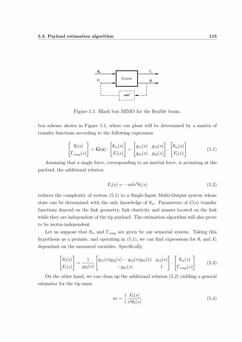
5.3. Payload estimation algorithm 115
-mls2
System
m
Ft t
!c
Figure 5.1: Black box MIMO for the flexible beam.
box scheme shown in Figure 5.1, where our plant will be determined by a matrix of
transfer functions according to the following expression
[
θt(s)
Γcoup(s)
]
= G(s) ·[
θm(s)
Ft(s)
]
=
[
g11(s) g12(s)
g21(s) g22(s)
]
·[
θm(s)
Ft(s)
]
(5.1)
Assuming that a single force, corresponding to an inertial force, is actuating at the
payload, the additional relation
Ft(s) = −mls2θt(s) (5.2)
reduces the complexity of system (5.1) to a Single-Input Multi-Output system whose
state can be determined with the only knowledge of θm. Parameters of G(s) transfer
functions depend on the link geometry, link elasticity and masses located on the link
while they are independent of the tip payload. The estimation algorithm will also prove
to be motor-independent.
Let us suppose that θm and Γcoup are given by our sensorial system. Taking this
hypothesis as a premise, and operating in (5.1), we can find expressions for θt and Ft
dependant on the measured variables. Specifically,
[
θt(s)
Ft(s)
]
=1
g22(s)
[
g11(s)g22(s)− g12(s)g21(s) g12(s)
−g21(s) 1
]
·[
θm(s)
Γcoup(s)
]
(5.3)
On the other hand, we can clean up the additional relation (5.2) yielding a general
estimator for the tip mass
m =1
l
Ft(s)
s2θt(s)(5.4)
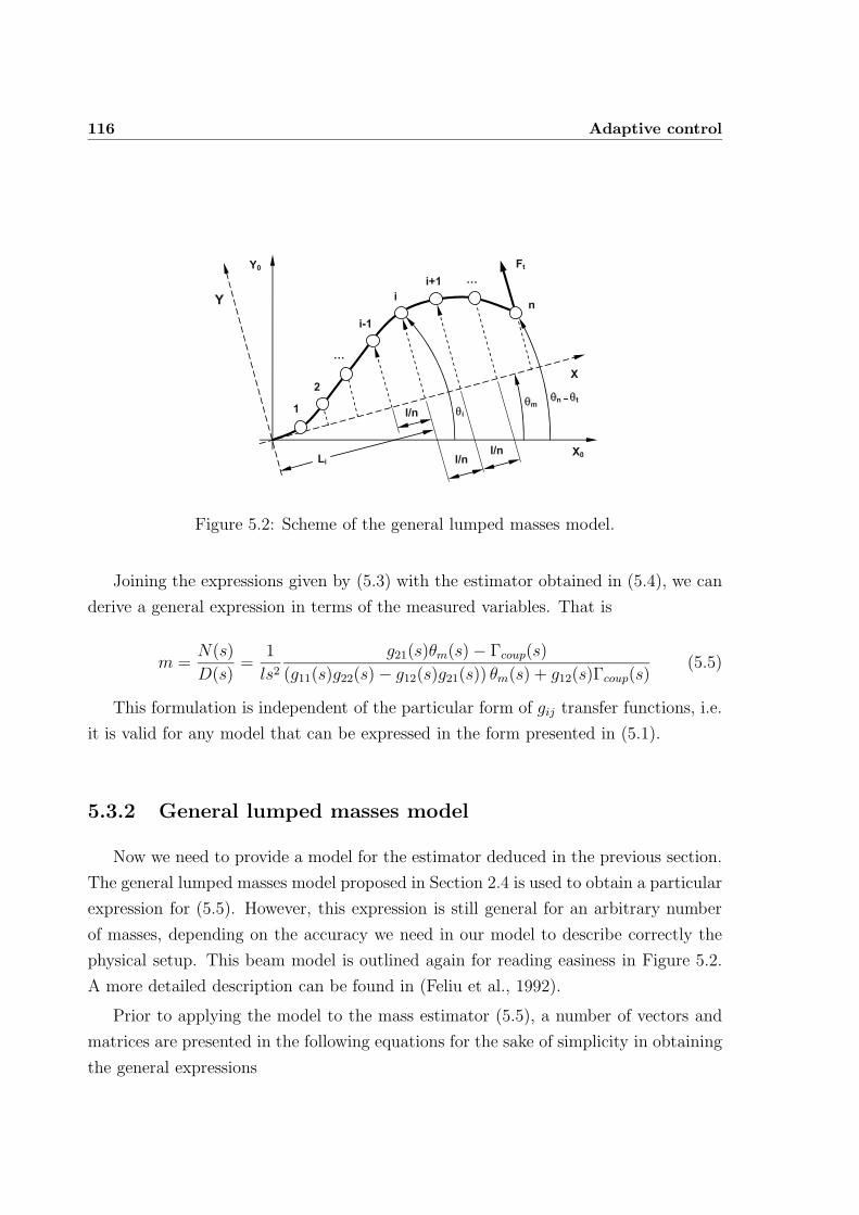
116 Adaptive control
2
i
i-1
i+1
1
n
…
…
Y
X
Y0
X0
Ft
m i
n
t
Li
l/n
l/n l/n
Figure 5.2: Scheme of the general lumped masses model.
Joining the expressions given by (5.3) with the estimator obtained in (5.4), we can
derive a general expression in terms of the measured variables. That is
m =N(s)
D(s)=
1
ls2g21(s)θm(s)− Γcoup(s)
(g11(s)g22(s)− g12(s)g21(s)) θm(s) + g12(s)Γcoup(s)(5.5)
This formulation is independent of the particular form of gij transfer functions, i.e.
it is valid for any model that can be expressed in the form presented in (5.1).
5.3.2 General lumped masses model
Now we need to provide a model for the estimator deduced in the previous section.
The general lumped masses model proposed in Section 2.4 is used to obtain a particular
expression for (5.5). However, this expression is still general for an arbitrary number
of masses, depending on the accuracy we need in our model to describe correctly the
physical setup. This beam model is outlined again for reading easiness in Figure 5.2.
A more detailed description can be found in (Feliu et al., 1992).
Prior to applying the model to the mass estimator (5.5), a number of vectors and
matrices are presented in the following equations for the sake of simplicity in obtaining
the general expressions
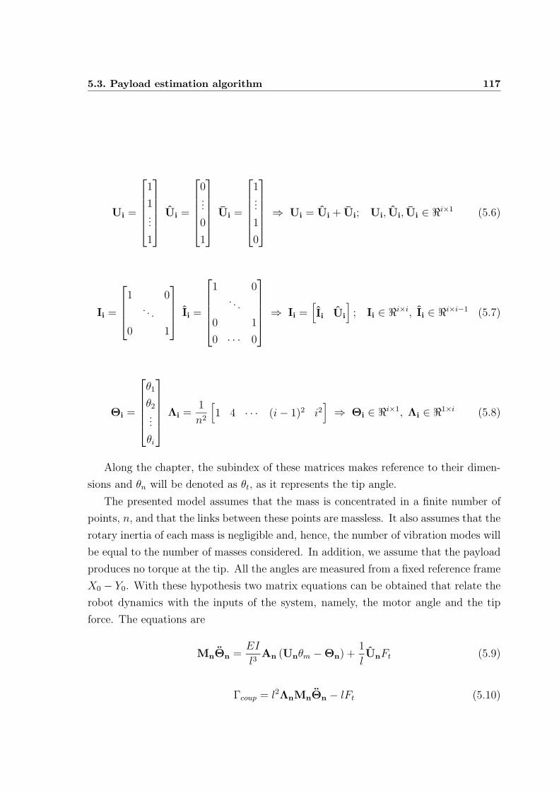
5.3. Payload estimation algorithm 117
Ui =
1
1...
1
Ui =
0...
0
1
Ui =
1...
1
0
⇒ Ui = Ui + Ui; Ui, Ui, Ui ∈ ℜi×1 (5.6)
Ii =
1 0. . .
0 1
Ii =
1 0. . .
0 1
0 · · · 0
⇒ Ii =[
Ii Ui
]
; Ii ∈ ℜi×i, Ii ∈ ℜi×i−1 (5.7)
Θi =
θ1
θ2...
θi
Λi =1
n2
[
1 4 · · · (i− 1)2 i2]
⇒ Θi ∈ ℜi×1, Λi ∈ ℜ1×i (5.8)
Along the chapter, the subindex of these matrices makes reference to their dimen-
sions and θn will be denoted as θt, as it represents the tip angle.
The presented model assumes that the mass is concentrated in a finite number of
points, n, and that the links between these points are massless. It also assumes that the
rotary inertia of each mass is negligible and, hence, the number of vibration modes will
be equal to the number of masses considered. In addition, we assume that the payload
produces no torque at the tip. All the angles are measured from a fixed reference frame
X0 − Y0. With these hypothesis two matrix equations can be obtained that relate the
robot dynamics with the inputs of the system, namely, the motor angle and the tip
force. The equations are
MnΘn =EI
l3An (Unθm −Θn) +
1
lUnFt (5.9)
Γcoup = l2ΛnMnΘn − lFt (5.10)
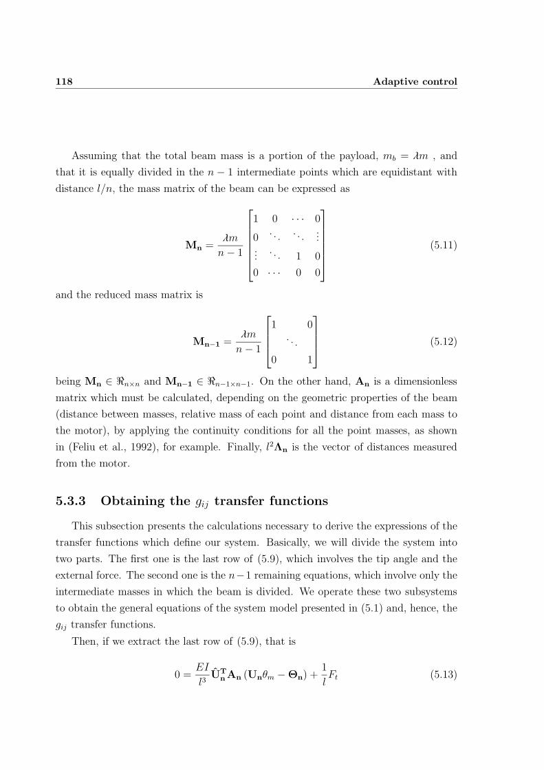
118 Adaptive control
Assuming that the total beam mass is a portion of the payload, mb = λm , and
that it is equally divided in the n − 1 intermediate points which are equidistant with
distance l/n, the mass matrix of the beam can be expressed as
Mn =λm
n− 1
1 0 · · · 0
0. . .
. . ....
.... . . 1 0
0 · · · 0 0
(5.11)
and the reduced mass matrix is
Mn−1 =λm
n− 1
1 0. . .
0 1
(5.12)
being Mn ∈ ℜn×n and Mn−1 ∈ ℜn−1×n−1. On the other hand, An is a dimensionless
matrix which must be calculated, depending on the geometric properties of the beam
(distance between masses, relative mass of each point and distance from each mass to
the motor), by applying the continuity conditions for all the point masses, as shown
in (Feliu et al., 1992), for example. Finally, l2Λn is the vector of distances measured
from the motor.
5.3.3 Obtaining the gij transfer functions
This subsection presents the calculations necessary to derive the expressions of the
transfer functions which define our system. Basically, we will divide the system into
two parts. The first one is the last row of (5.9), which involves the tip angle and the
external force. The second one is the n−1 remaining equations, which involve only the
intermediate masses in which the beam is divided. We operate these two subsystems
to obtain the general equations of the system model presented in (5.1) and, hence, the
gij transfer functions.
Then, if we extract the last row of (5.9), that is
0 =EI
l3UT
nAn (Unθm −Θn) +
1
lFt (5.13)
5.3. Payload estimation algorithm 119
and then we rearrange the equation making use of the definitions given in (5.6), (5.7)
and (5.8), we obtain the following expression for the tip angle
θt = θm +UT
nAnIn
UTnAnUn
(Un−1θm −Θn−1) +1
UTnAnUn
l2
EIFt (5.14)
where UT
nrepresents the transpose of Un.
Taking into consideration only the first n− 1 equations, expression (5.9) yields
Mn−1Θn−1 =EI
l3ITnAn (Unθm −Θn) =
EI
l3ITnAn
(
Unθm − InΘn−1 − Unθt
)
(5.15)
Substituting the value of θt given by (5.14) into the previous equation, and rear-
ranging terms, we obtain
Θn−1 =n− 1
λm
EI
l3ITnAn
(
In − Un
UT
nAn
UTnAnUn
)
In (Unθm −Θn)−n− 1
λm
ITnAnUn
UTnAnUn
Ft
(5.16)
which can be shortened to
Θn−1 =n− 1
λm
EI
l3An−1 (Unθm −Θn)−
n− 1
λmPn−1Ft (5.17)
where two new matrixes are defined
An−1 = ITnAn
(
In − Un
UT
nAn
UTnAnUn
)
In, An−1 ∈ ℜn−1×n−1 (5.18a)
Pn−1 =ITnAnUn
UTnAnUn
, Pn−1 ∈ ℜn−1×1 (5.18b)
Transforming (5.17) into the Laplace domain, we have
Θn−1(s) =
(
In−1
s2
ω2+An−1
)−1
An−1Un−1θm(s)−l2
EI
(
In−1
s2
ω2+An−1
)−1
Pn−1Ft(s)
(5.19)
120 Adaptive control
where
ω2 =n− 1
λm
EI
l3=
(n− 1)EI
mbl3(5.20)
Finally, substituting (5.19) in (5.14) and reordering the resultant equation, we
achieve an expression which relates the tip angle with measured variables, coupling
torque and motor angle, i.e. the first equation of the general model presented
θt(s) =UT
nAn
UTnAnUn
(
Un − In
(
In−1
s2
ω2+An−1
)−1
An−1Un−1
)
θm(s)+
+l2
EI
1
UTnAnUn
(
UT
nAnIn
(
In−1
s2
ω2+An−1
)−1
Pn−1 + 1
)
Ft(s) (5.21)
On the other hand, we can rewrite (5.10) in the Laplace domain as
Γcoup(s) = l2Λn−1Mn−1s2Θn−1(s)− lFt(s) (5.22)
and, substituting (5.12) and (5.19) in the previous relation, we obtain the expression
for Γcoup(s) in terms of θm(s) and Ft(s), completing the model proposed in (5.1)
Γcoup(s) =
(
EI
l
s2
ω2Λn−1
(
In−1
s2
ω2+An−1
)−1
An−1Un−1
)
θm(s)−
−(
s2
ω2Λn−1
(
In−1
s2
ω2+An−1
)−1
Pn−1 + 1
)
lFt(s) (5.23)
Therefore, it is immediate to deduce the values of the transfer functions in G(s),
which are
5.4. Particular cases 121
G(s) =
[
g11(s) g12(s)
g21(s) g22(s)
]
⇒
⇒
g11(s) =UT
nAn
UTnAnUn
(
Un − In
(
In−1
s2
ω2+An−1
)−1
An−1Un−1
)
g12(s) =l2
EI
1
UTnAnUn
(
UT
nAnIn
(
In−1
s2
ω2+An−1
)−1
Pn−1 + 1
)
g21(s) =
(
EI
l
s2
ω2Λn−1
(
In−1
s2
ω2+An−1
)−1
An−1Un−1
)
g22(s) = −l
(
s2
ω2Λn−1
(
In−1
s2
ω2+An−1
)−1
Pn−1 + 1
)
(5.24)
5.4 Particular cases
To illustrate the previous mathematical results, this section presents two particular
cases: a beam whose mass can be neglected; and a beam with its mass concentrated
at its middle point.
5.4.1 Beam with negligible mass
In this case, the matrix form of the dynamic model of the system presented in (5.5)
and (5.9) collapses into the two following scalar equations
0 =3EI
l3(θm − θt) +
1
lFt (5.25)
Γcoup = −lFt (5.26)
The matrices of the system are
Mn = 0; An = 3; Un = 1; Un = 0; In = ∅;
Mn−1 = ∅; An−1 = ∅; Un−1 = ∅; Un = 0; Pn−1 = ∅;
(5.27)
122 Adaptive control
where ∅ indicates that a matrix has dimension zero. These matrixes yield the following
transfer functions
G(s) =
1
l2
3EI0 −l
(5.28)
Substituting in (5.5), the mass estimator for a very lightweight beam yields
m =1
l2s2Γcoup(s)
θm(s)−l
3EIΓcoup(s)
(5.29)
and, applying the inverse Laplace transformation, we obtain an expression in the time
domain
m =1
l2Γcoup(t)
θm(t)−Γcoup(t)
c
(5.30)
where c = 3EIl
is the stiffness of the beam, which is supposed massless.
5.4.2 Beam with its mass concentrated in a single point
Now we particularize the estimator for a beam model assuming the mass to be
concentrated in its middle point. For this particular case the matrices of the model are
Mn = λm
[
1 0
0 0
]
; An =24
7
[
32 −20
−5 4
]
; Un =
[
1
1
]
; Un =
[
0
1
]
; In =
[
1
0
]
;
Mn−1 = λm; An−1 = 24; Un−1 = 1; ; Un =
[
1
0
]
; Pn−1 = −5;
(5.31)
Therefore, the transfer functions yield
5.4. Particular cases 123
G(s) =
−14s2 + 24ω2
s2 + 24ω2
l2
EI
796s2 + 8ω2
s2 + 24ω2
2cs2
s2 + 24ω2l14s2 + 24ω2
s2 + 24ω2
(5.32)
Then, substituting in (5.5), we obtain the expression of the mass estimator for this
particular beam model, resulting
m =1
l2s2
2cs2
s2 + 24ω2θm(s)− Γcoup(s)
−l12s2 + 24ω2
s2 + 24ω2θm(s) +
l2
3EI
796s2 + 8ω2
s2 + 24ω2Γcoup(s)
=
=1
l2
Γcoup(s)−2cs2
s2 + 24ω2θm(s)
12s2 + 24ω2
s2 + 24ω2θm(s)−
732s2 + 24ω2
s2 + 24ω2
Γcoup(s)
c
(5.33)
Comparing (5.30) and (5.33), it is evident that the use of a more complete model
increases the complexity of the estimator to a large extent, involving more demand-
ing calculations. However, both expressions are related and it is demonstrable that
(5.30) is a particular case of (5.33), by calculating the limit for this last expression
when mb tends to zero, and therefore ω tends to infinity, as can be deducted from
expression (5.20).
5.4.3 Filtering the estimator
In any of the estimators derived from (5.5) we need the second derivative of motor
angle and coupling torque, and it is well known that differentiating noisy signals, as the
measurements obtained from a strain gauge, does not give a good result. Accordingly,
it is not advisable to use expressions (5.30) and (5.33) in that raw form, because the
gauge signal could lead us to an erroneous identification.
It is convenient to filter that signal in order to obtain correct results. Hence, we
modify the general expression of the estimation (5.5) by multiplying its numerator and
denominator by the same transfer function F (s), corresponding to a low-pass filter,
124 Adaptive control
to secure a smoother signal for the mass estimation. This manner of filtering the
signal does not alter the speed of convergence of the estimator while makes the output
smoother. The pass-band filter has been discarded due to the low oscillation frequencies
of our mechanical system, as the response would become very slow.
The filtered signals will be denoted with a tilde. Their transfer functions, trans-
formed into the Laplace domain, yield
N(s) = F (s) ·N(s) =
(ωf
s+ ωf
)2
(g21(s)θm(s)− Γcoup(s)) (5.34)
D(s) = F (s)·D(s) = l2s2(
ωf
s+ ωf
)2
((g11(s)g22(s)− g12(s)g21(s)) θm(s) + g12(s)Γcoup(s))
(5.35)
where ωf represents the cut-off frequency (in rad/sec) of the filter. The ωf selection
will rely on the knowledge of the physical system, that is, on the range of variation
of the system natural frequencies. Specifically, it will be set to half decade over the
highest of these frequencies. The order of the filter has been inferred from numerical
simulations as a trade-off between attenuation of noise and small interference on the
original signals.
In the denominator of (5.35), the second derivative has been included into the filter
solving the problems with the noisy signals. Then, we can calculate the equivalent
expression in the Z-domain (Ogata, 2001) for the parenthesis in (5.34), (first order
filter), and then raise to square, thereby obtaining the following discretized expression
for the second order filter
F1(z) = Z
(ωf
s+ ωf
)
=∑
at poles of G(p)
Residues of
(ωf
p + ωf
1
1− epT z−1
)
⇒
⇒ F (z) = F 21 (z) =
(1− e−ωfT
)2
z2 − 2e−ωfT z + e−2ωfT(5.36)
where Z [·] represents the Z-transform of an expression.
In the denominator, making use of the properties of the Z-transform, the filter yields
5.5. Simulation results 125
Z(s2F (s)
) ∼=(1− z−1
T
)2
F (z) ⇒ Z(s2F (s)
) ∼=
1
T 2
(1− e−ωfT
)2(z2 − 2z − 1)
z2 − 2e−ωfT z + e−2ωfT
(5.37)
This filter also limits the bandwidth of the measured signals used in the estimation
of the mass. Therefore, if we adjust appropriately the cut-off frequency, ωf , we can
attenuate the measurement of the high frequency modes so that only the first mode
passes the filter, the single mass estimator becoming then valid for any model. This is
a nice property which is illustrated in the simulations section.
5.5 Simulation results
This section verifies the properties of the proposed identification scheme: low esti-
mation time and good accuracy. First the goodness of the estimation is corroborated
and, once the estimation is approved, the adaptive algorithm, based on simple PD
controllers whose constants are updated depending on payload values, is also tested
numerically. The data used for these latter simulations, correspond to the carbon fiber
link platform defined in Section 2.6.2.
5.5.1 Estimation algorithm
This section studies the performance of the identification process using three differ-
ent models for the flexible link (all of them presented in Chapter 2) and two different
estimators (presented in Section 5.4).
Simulation block diagram is displayed in Figure 5.3, where the M(s) represents
the equivalent transfer function of the actuator control loop. As described in Chapter
2, the DC motor rotates the beam to the desired position and it is driven by means
of an amplifier acting as a current controller, whose control signal, V , varies between
+2V and -2V. Motor dynamics and inner control loop were previously discussed in
Section 3.2.1.
The parameters of the PD controller in the inner control loop have been calculated
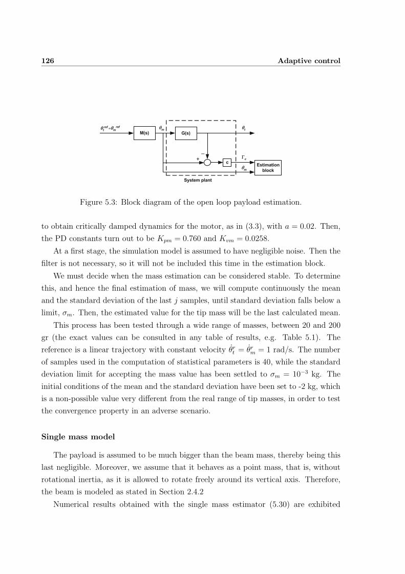
126 Adaptive control
M(s) G(s)
m
t
c
t
ref
+
!m
ref
_
System plant
Estimation
block
c
m
Figure 5.3: Block diagram of the open loop payload estimation.
to obtain critically damped dynamics for the motor, as in (3.3), with a = 0.02. Then,
the PD constants turn out to be Kpm = 0.760 and Kvm = 0.0258.
At a first stage, the simulation model is assumed to have negligible noise. Then the
filter is not necessary, so it will not be included this time in the estimation block.
We must decide when the mass estimation can be considered stable. To determine
this, and hence the final estimation of mass, we will compute continuously the mean
and the standard deviation of the last j samples, until standard deviation falls below a
limit, σm. Then, the estimated value for the tip mass will be the last calculated mean.
This process has been tested through a wide range of masses, between 20 and 200
gr (the exact values can be consulted in any table of results, e.g. Table 5.1). The
reference is a linear trajectory with constant velocity θrt = θrm = 1 rad/s. The number
of samples used in the computation of statistical parameters is 40, while the standard
deviation limit for accepting the mass value has been settled to σm = 10−3 kg. The
initial conditions of the mean and the standard deviation have been set to -2 kg, which
is a non-possible value very different from the real range of tip masses, in order to test
the convergence property in an adverse scenario.
Single mass model
The payload is assumed to be much bigger than the beam mass, thereby being this
last negligible. Moreover, we assume that it behaves as a point mass, that is, without
rotational inertia, as it is allowed to rotate freely around its vertical axis. Therefore,
the beam is modeled as stated in Section 2.4.2
Numerical results obtained with the single mass estimator (5.30) are exhibited
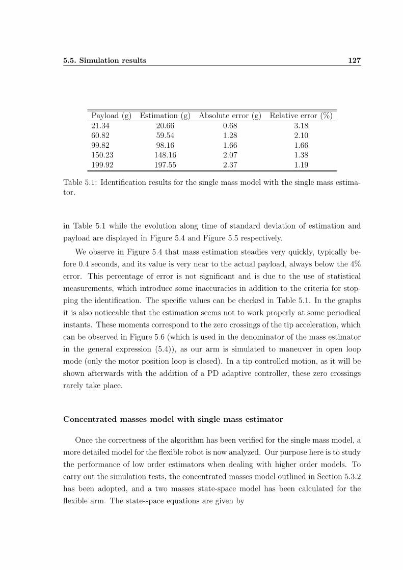
5.5. Simulation results 127
Payload (g) Estimation (g) Absolute error (g) Relative error (%)21.34 20.66 0.68 3.1860.82 59.54 1.28 2.1099.82 98.16 1.66 1.66150.23 148.16 2.07 1.38199.92 197.55 2.37 1.19
Table 5.1: Identification results for the single mass model with the single mass estima-tor.
in Table 5.1 while the evolution along time of standard deviation of estimation and
payload are displayed in Figure 5.4 and Figure 5.5 respectively.
We observe in Figure 5.4 that mass estimation steadies very quickly, typically be-
fore 0.4 seconds, and its value is very near to the actual payload, always below the 4%
error. This percentage of error is not significant and is due to the use of statistical
measurements, which introduce some inaccuracies in addition to the criteria for stop-
ping the identification. The specific values can be checked in Table 5.1. In the graphs
it is also noticeable that the estimation seems not to work properly at some periodical
instants. These moments correspond to the zero crossings of the tip acceleration, which
can be observed in Figure 5.6 (which is used in the denominator of the mass estimator
in the general expression (5.4)), as our arm is simulated to maneuver in open loop
mode (only the motor position loop is closed). In a tip controlled motion, as it will be
shown afterwards with the addition of a PD adaptive controller, these zero crossings
rarely take place.
Concentrated masses model with single mass estimator
Once the correctness of the algorithm has been verified for the single mass model, a
more detailed model for the flexible robot is now analyzed. Our purpose here is to study
the performance of low order estimators when dealing with higher order models. To
carry out the simulation tests, the concentrated masses model outlined in Section 5.3.2
has been adopted, and a two masses state-space model has been calculated for the
flexible arm. The state-space equations are given by
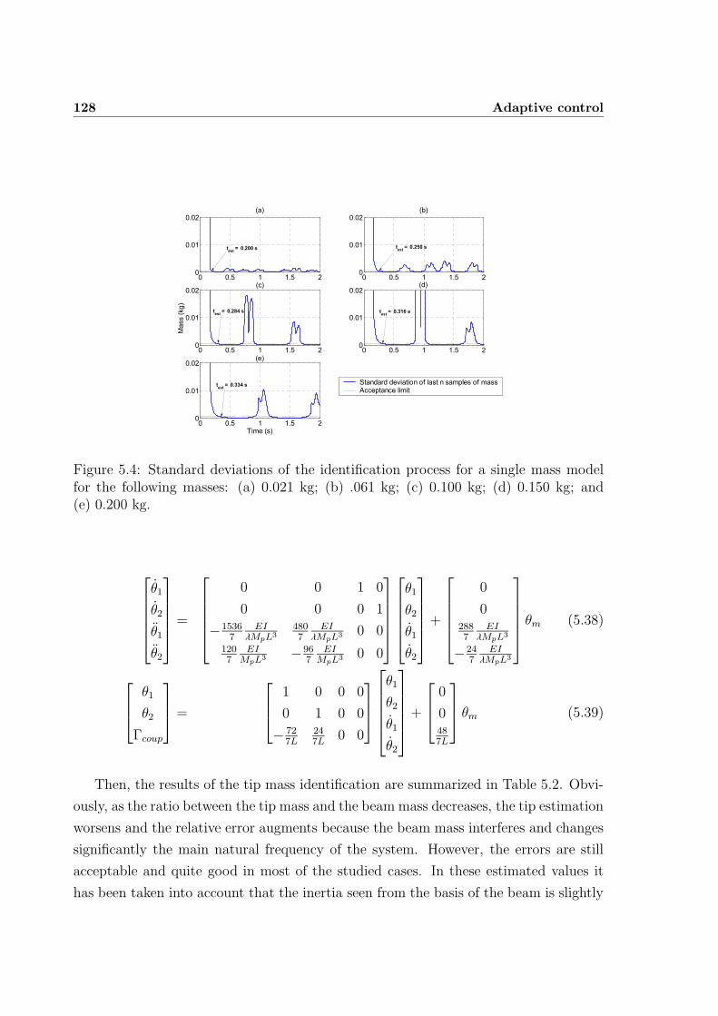
128 Adaptive control
0 0.5 1 1.5 20
0.01
0.02(a)
0 0.5 1 1.5 20
0.01
0.02(b)
0 0.5 1 1.5 20
0.01
0.02(c)
Mass (
kg)
0 0.5 1 1.5 20
0.01
0.02(d)
0 0.5 1 1.5 20
0.01
0.02(e)
Time (s)
Standard deviation of last n samples of massAcceptance limit
test
= 0.200 s test
= 0.250 s
test
= 0.284 s test
= 0.316 s
test
= 0.334 s
Figure 5.4: Standard deviations of the identification process for a single mass modelfor the following masses: (a) 0.021 kg; (b) .061 kg; (c) 0.100 kg; (d) 0.150 kg; and(e) 0.200 kg.
θ1
θ2
θ1
θ2
=
0 0 1 0
0 0 0 1
−15367
EIλMpL3
4807
EIλMpL3 0 0
1207
EIMpL3 −96
7EI
MpL3 0 0
θ1
θ2
θ1
θ2
+
0
02887
EIλMpL3
−247
EIλMpL3
θm (5.38)
θ1
θ2
Γcoup
=
1 0 0 0
0 1 0 0
− 727L
247L
0 0
θ1
θ2
θ1
θ2
+
0
0487L
θm (5.39)
Then, the results of the tip mass identification are summarized in Table 5.2. Obvi-
ously, as the ratio between the tip mass and the beam mass decreases, the tip estimation
worsens and the relative error augments because the beam mass interferes and changes
significantly the main natural frequency of the system. However, the errors are still
acceptable and quite good in most of the studied cases. In these estimated values it
has been taken into account that the inertia seen from the basis of the beam is slightly
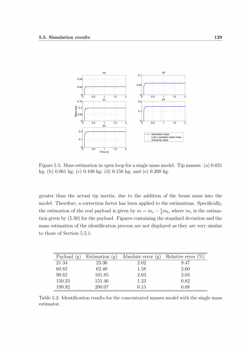
5.5. Simulation results 129
0 0.5 1 1.5 20
0.02
0.04
(a)
0 0.5 1 1.5 20
0.05
0.1(b)
0 0.5 1 1.5 20
0.05
0.1
0.15(c)
Mass (
kg)
0 0.5 1 1.5 20
0.1
0.2(d)
0 0.5 1 1.5 20
0.1
0.2
(e)
Time (s)
Estimated massLast n samples mean massActual tip mass
Figure 5.5: Mass estimation in open loop for a single mass model. Tip masses: (a) 0.021kg; (b) 0.061 kg; (c) 0.100 kg; (d) 0.150 kg; and (e) 0.200 kg.
greater than the actual tip inertia, due to the addition of the beam mass into the
model. Therefore, a correction factor has been applied to the estimations. Specifically,
the estimation of the real payload is given by m = me − 14mb, where me is the estima-
tion given by (5.30) for the payload. Figures containing the standard deviation and the
mass estimation of the identification process are not displayed as they are very similar
to those of Section 5.5.1.
Payload (g) Estimation (g) Absolute error (g) Relative error (%)21.34 23.36 2.02 9.4760.82 62.40 1.58 2.6099.82 101.85 2.03 2.03150.23 151.46 1.23 0.82199.92 200.07 0.15 0.08
Table 5.2: Identification results for the concentrated masses model with the single massestimator.
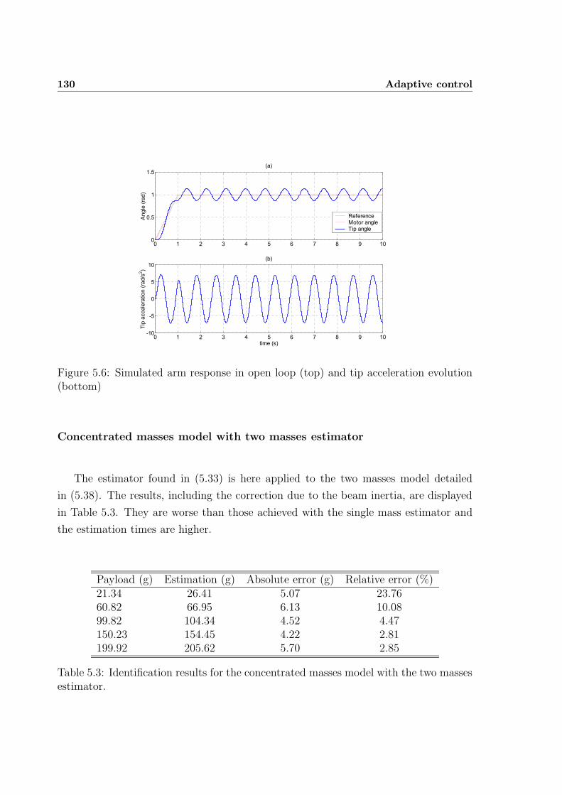
130 Adaptive control
0 1 2 3 4 5 6 7 8 9 100
0.5
1
1.5
Angle
(ra
d)
ReferenceMotor angleTip angle
0 1 2 3 4 5 6 7 8 9 10-10
-5
0
5
10
Tip
accele
ration (
rad/s
2)
time (s)
(a)
(b)
Figure 5.6: Simulated arm response in open loop (top) and tip acceleration evolution(bottom)
Concentrated masses model with two masses estimator
The estimator found in (5.33) is here applied to the two masses model detailed
in (5.38). The results, including the correction due to the beam inertia, are displayed
in Table 5.3. They are worse than those achieved with the single mass estimator and
the estimation times are higher.
Payload (g) Estimation (g) Absolute error (g) Relative error (%)21.34 26.41 5.07 23.7660.82 66.95 6.13 10.0899.82 104.34 4.52 4.47150.23 154.45 4.22 2.81199.92 205.62 5.70 2.85
Table 5.3: Identification results for the concentrated masses model with the two massesestimator.
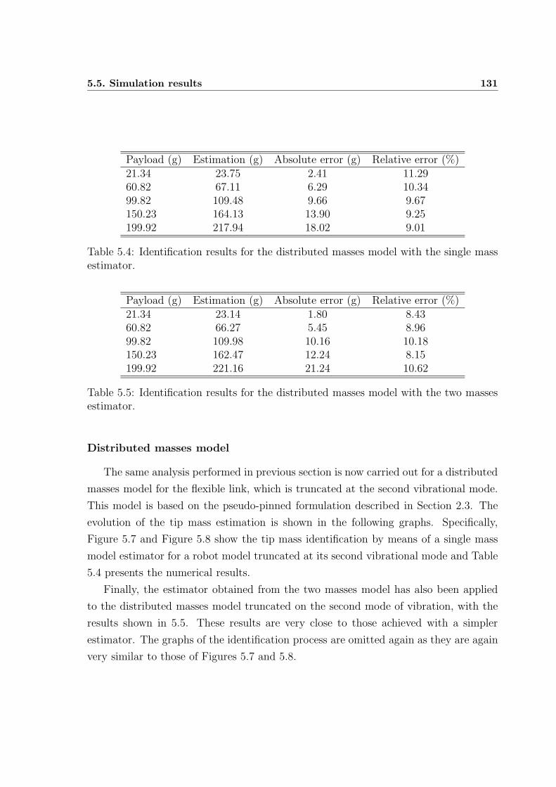
5.5. Simulation results 131
Payload (g) Estimation (g) Absolute error (g) Relative error (%)21.34 23.75 2.41 11.2960.82 67.11 6.29 10.3499.82 109.48 9.66 9.67150.23 164.13 13.90 9.25199.92 217.94 18.02 9.01
Table 5.4: Identification results for the distributed masses model with the single massestimator.
Payload (g) Estimation (g) Absolute error (g) Relative error (%)21.34 23.14 1.80 8.4360.82 66.27 5.45 8.9699.82 109.98 10.16 10.18150.23 162.47 12.24 8.15199.92 221.16 21.24 10.62
Table 5.5: Identification results for the distributed masses model with the two massesestimator.
Distributed masses model
The same analysis performed in previous section is now carried out for a distributed
masses model for the flexible link, which is truncated at the second vibrational mode.
This model is based on the pseudo-pinned formulation described in Section 2.3. The
evolution of the tip mass estimation is shown in the following graphs. Specifically,
Figure 5.7 and Figure 5.8 show the tip mass identification by means of a single mass
model estimator for a robot model truncated at its second vibrational mode and Table
5.4 presents the numerical results.
Finally, the estimator obtained from the two masses model has also been applied
to the distributed masses model truncated on the second mode of vibration, with the
results shown in 5.5. These results are very close to those achieved with a simpler
estimator. The graphs of the identification process are omitted again as they are again
very similar to those of Figures 5.7 and 5.8.
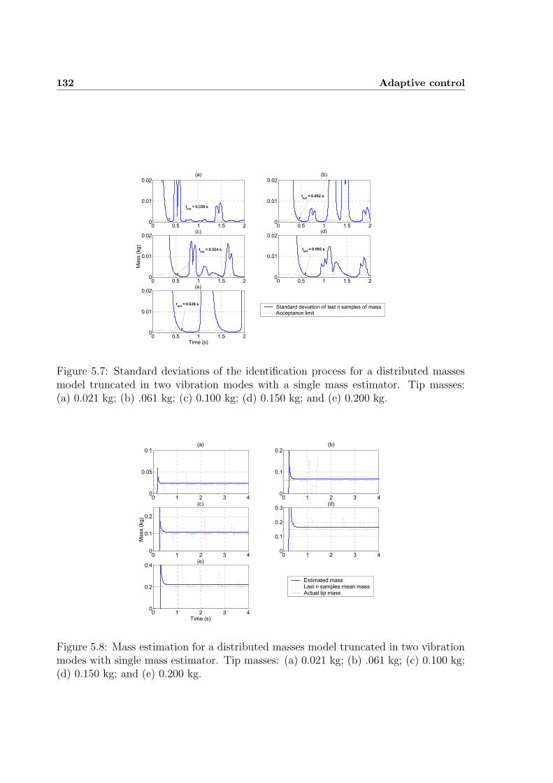
132 Adaptive control
0 0.5 1 1.5 20
0.01
0.02(a)
0 0.5 1 1.5 20
0.01
0.02(b)
0 0.5 1 1.5 20
0.01
0.02(c)
Mass (
kg)
0 0.5 1 1.5 20
0.01
0.02(d)
0 0.5 1 1.5 20
0.01
0.02(e)
Time (s)
Standard deviation of last n samples of massAcceptance limit
test
= 0.330 s
test
= 0.452 s
test
= 0.524 s test
= 0.592 s
test
= 0.638 s
Figure 5.7: Standard deviations of the identification process for a distributed massesmodel truncated in two vibration modes with a single mass estimator. Tip masses:(a) 0.021 kg; (b) .061 kg; (c) 0.100 kg; (d) 0.150 kg; and (e) 0.200 kg.
0 1 2 3 40
0.05
0.1(a)
0 1 2 3 40
0.1
0.2(b)
0 1 2 3 40
0.1
0.2
(c)
Mass (
kg)
0 1 2 3 40
0.1
0.2
0.3(d)
0 1 2 3 40
0.2
0.4(e)
Time (s)
Estimated massLast n samples mean massActual tip mass
Figure 5.8: Mass estimation for a distributed masses model truncated in two vibrationmodes with single mass estimator. Tip masses: (a) 0.021 kg; (b) .061 kg; (c) 0.100 kg;(d) 0.150 kg; and (e) 0.200 kg.
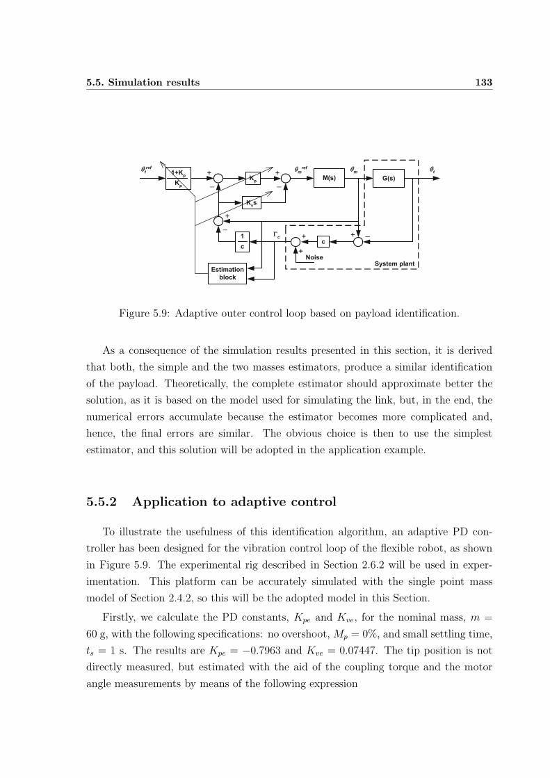
5.5. Simulation results 133
M(s) G(s)
m
t
Kvs
Kp
c1
c
1+Kp
Kp
t
ref
+ +
+
+
+
+
m
ref
Noise
_
_
_
_
System plant
c
Estimation
block
Figure 5.9: Adaptive outer control loop based on payload identification.
As a consequence of the simulation results presented in this section, it is derived
that both, the simple and the two masses estimators, produce a similar identification
of the payload. Theoretically, the complete estimator should approximate better the
solution, as it is based on the model used for simulating the link, but, in the end, the
numerical errors accumulate because the estimator becomes more complicated and,
hence, the final errors are similar. The obvious choice is then to use the simplest
estimator, and this solution will be adopted in the application example.
5.5.2 Application to adaptive control
To illustrate the usefulness of this identification algorithm, an adaptive PD con-
troller has been designed for the vibration control loop of the flexible robot, as shown
in Figure 5.9. The experimental rig described in Section 2.6.2 will be used in exper-
imentation. This platform can be accurately simulated with the single point mass
model of Section 2.4.2, so this will be the adopted model in this Section.
Firstly, we calculate the PD constants, Kpe and Kve, for the nominal mass, m =
60 g, with the following specifications: no overshoot, Mp = 0%, and small settling time,
ts = 1 s. The results are Kpe = −0.7963 and Kve = 0.07447. The tip position is not
directly measured, but estimated with the aid of the coupling torque and the motor
angle measurements by means of the following expression
134 Adaptive control
θte = θm − Γcoup
c(5.40)
which is obtained from (2.37).
A noise term is added to the coupling torque to simulate the experimental measures
of the strain gauges, which are very noisy. From the experimental measurement of our
sensing system, the variance of this noise have been set to 10−5 Nm. Therefore, we now
need to filter the mass estimation as explained in Section 5.4.3. The selected cut-off
frequency for the estimator filter is ωf = 10 rad/s, what, applied to (5.36) and (5.37),
and particularized for the a sample time T = 0.002 s, yields
F (s) =
(10
s+ 10
)2
⇒ Z (F (s))T=0.002∼=
0.01982z2
z2 − 1.961z + 0.961(5.41)
Z(s2F (s)
)
T=0.002∼=
98.0232z2 − 196.046z + 98.023
z2 − 1.961z + 0.961(5.42)
Now we will perform the maneuvers for each of the masses considered for the system,
that is, from three times lighter than nominal, mm = 20 g, to more than three times
heavier, mM = 202 g. In Figure 5.10 the tip mass position during the maneuver when
using the PD controller for the nominal case is displayed. It is noticeable the high
overshoot that appears for payloads bigger than nominal, reaching the 14% for the
200 g mass. On the other side, the lightest mass performs slightly slower than the
nominal one. These results advise the use of a control scheme insensitive to payload
variations, such as adaptive control, to fulfill the requirements imposed to the system
for the whole range of masses. Figure 5.11 shows the control signal applied for each
simulation. Due to the noisy nature of these signals, it is very difficult to discriminate
any differences between the different masses. This voltage control is actually very
similar for all of them, but slightly delayed in time for the bigger masses.
Taking advantage of the identification algorithm (5.30), we will determine the ap-
propriate controller for each experiment. The simulation begins with the nominal PD
parameters and, whenever the estimation process finishes, these parameters are tuned
according to the actual payload, as shown in Table 5.6. In case the estimated mass
were not one of the those values, it would be obtained by linear interpolation. The
results are displayed from Figure 5.12 to Figure 5.14. From comparing the system re-
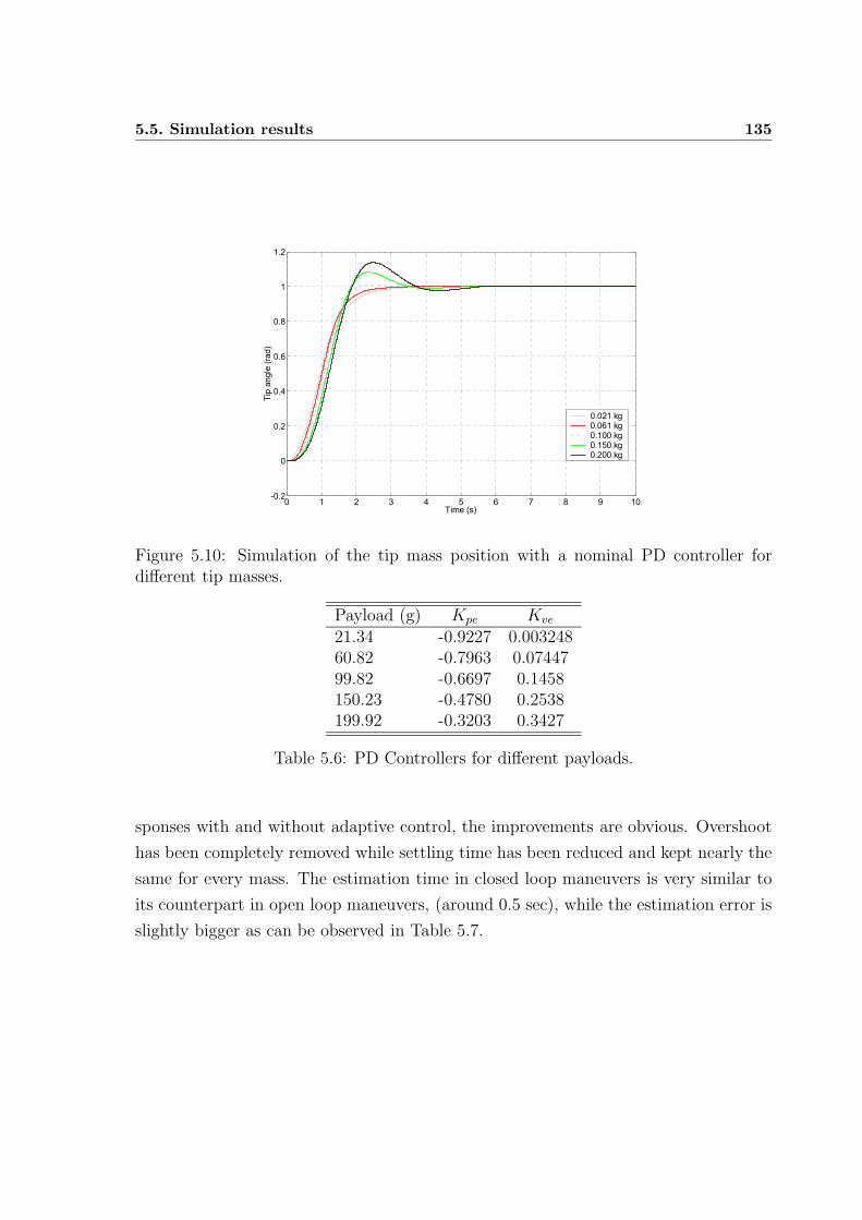
5.5. Simulation results 135
0 1 2 3 4 5 6 7 8 9 10-0.2
0
0.2
0.4
0.6
0.8
1
1.2
Time (s)
Tip
angle
(ra
d)
0.021 kg0.061 kg0.100 kg0.150 kg0.200 kg
Figure 5.10: Simulation of the tip mass position with a nominal PD controller fordifferent tip masses.
Payload (g) Kpe Kve
21.34 -0.9227 0.00324860.82 -0.7963 0.0744799.82 -0.6697 0.1458150.23 -0.4780 0.2538199.92 -0.3203 0.3427
Table 5.6: PD Controllers for different payloads.
sponses with and without adaptive control, the improvements are obvious. Overshoot
has been completely removed while settling time has been reduced and kept nearly the
same for every mass. The estimation time in closed loop maneuvers is very similar to
its counterpart in open loop maneuvers, (around 0.5 sec), while the estimation error is
slightly bigger as can be observed in Table 5.7.
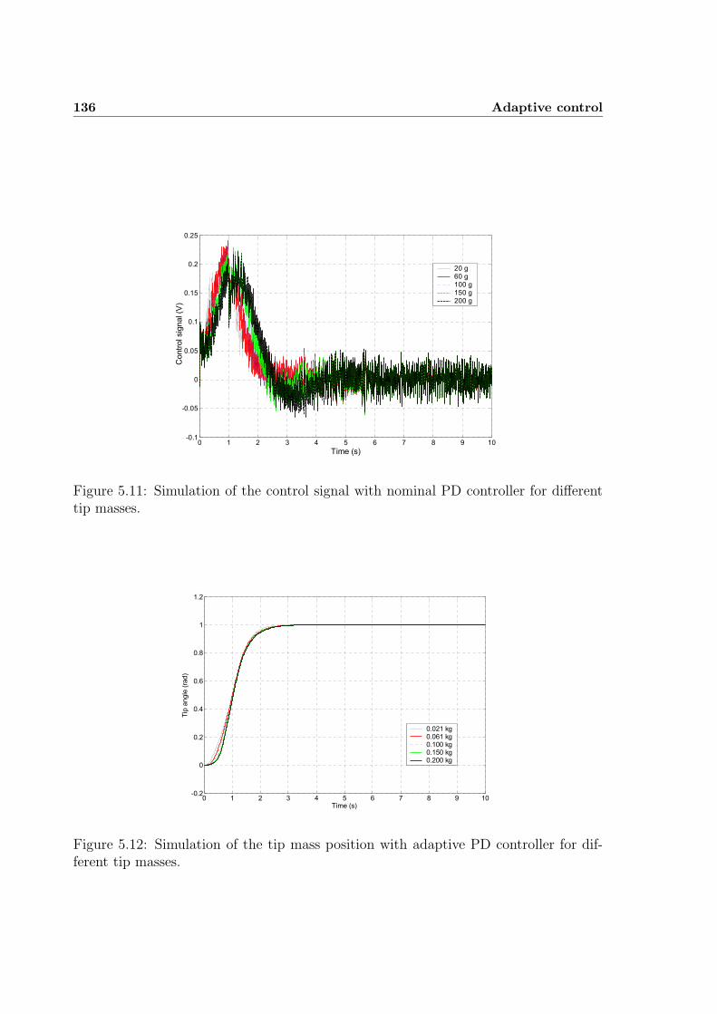
136 Adaptive control
0 1 2 3 4 5 6 7 8 9 10-0.1
-0.05
0
0.05
0.1
0.15
0.2
0.25
Time (s)
Contr
ol sig
nal (V
)
20 g60 g100 g150 g200 g
Figure 5.11: Simulation of the control signal with nominal PD controller for differenttip masses.
0 1 2 3 4 5 6 7 8 9 10-0.2
0
0.2
0.4
0.6
0.8
1
1.2
Time (s)
Tip
angle
(ra
d)
0.021 kg0.061 kg0.100 kg0.150 kg0.200 kg
Figure 5.12: Simulation of the tip mass position with adaptive PD controller for dif-ferent tip masses.
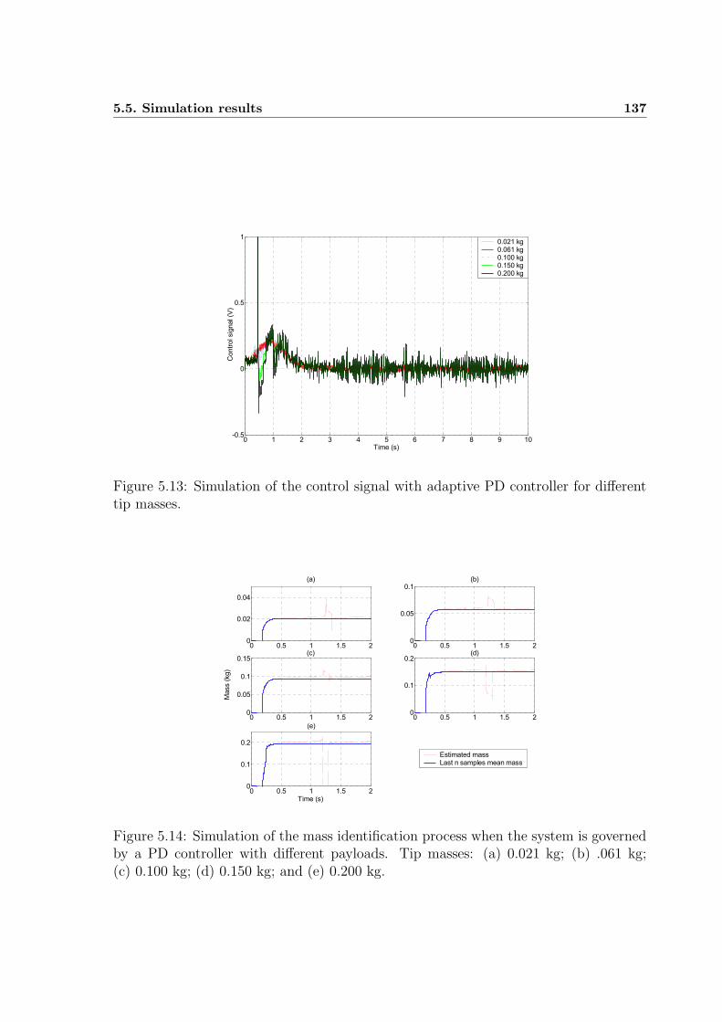
5.5. Simulation results 137
0 1 2 3 4 5 6 7 8 9 10-0.5
0
0.5
1
Time (s)
Contr
ol sig
nal (V
)
0.021 kg0.061 kg0.100 kg0.150 kg0.200 kg
Figure 5.13: Simulation of the control signal with adaptive PD controller for differenttip masses.
0 0.5 1 1.5 20
0.02
0.04
(a)
0 0.5 1 1.5 20
0.05
0.1(b)
0 0.5 1 1.5 20
0.05
0.1
0.15
Mass (
kg)
(c)
0 0.5 1 1.5 20
0.1
0.2(d)
0 0.5 1 1.5 20
0.1
0.2
Time (s)
(e)
Estimated massLast n samples mean mass
Figure 5.14: Simulation of the mass identification process when the system is governedby a PD controller with different payloads. Tip masses: (a) 0.021 kg; (b) .061 kg;(c) 0.100 kg; (d) 0.150 kg; and (e) 0.200 kg.
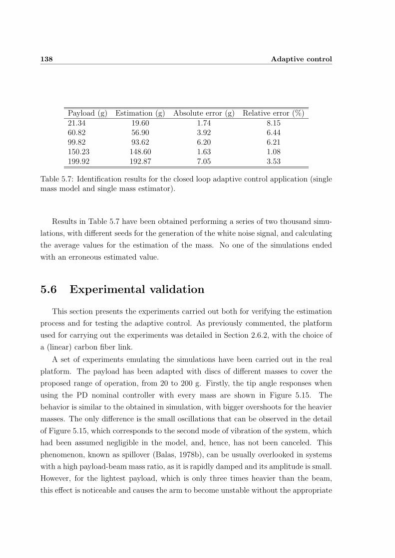
138 Adaptive control
Payload (g) Estimation (g) Absolute error (g) Relative error (%)21.34 19.60 1.74 8.1560.82 56.90 3.92 6.4499.82 93.62 6.20 6.21150.23 148.60 1.63 1.08199.92 192.87 7.05 3.53
Table 5.7: Identification results for the closed loop adaptive control application (singlemass model and single mass estimator).
Results in Table 5.7 have been obtained performing a series of two thousand simu-
lations, with different seeds for the generation of the white noise signal, and calculating
the average values for the estimation of the mass. No one of the simulations ended
with an erroneous estimated value.
5.6 Experimental validation
This section presents the experiments carried out both for verifying the estimation
process and for testing the adaptive control. As previously commented, the platform
used for carrying out the experiments was detailed in Section 2.6.2, with the choice of
a (linear) carbon fiber link.
A set of experiments emulating the simulations have been carried out in the real
platform. The payload has been adapted with discs of different masses to cover the
proposed range of operation, from 20 to 200 g. Firstly, the tip angle responses when
using the PD nominal controller with every mass are shown in Figure 5.15. The
behavior is similar to the obtained in simulation, with bigger overshoots for the heavier
masses. The only difference is the small oscillations that can be observed in the detail
of Figure 5.15, which corresponds to the second mode of vibration of the system, which
had been assumed negligible in the model, and, hence, has not been canceled. This
phenomenon, known as spillover (Balas, 1978b), can be usually overlooked in systems
with a high payload-beam mass ratio, as it is rapidly damped and its amplitude is small.
However, for the lightest payload, which is only three times heavier than the beam,
this effect is noticeable and causes the arm to become unstable without the appropriate
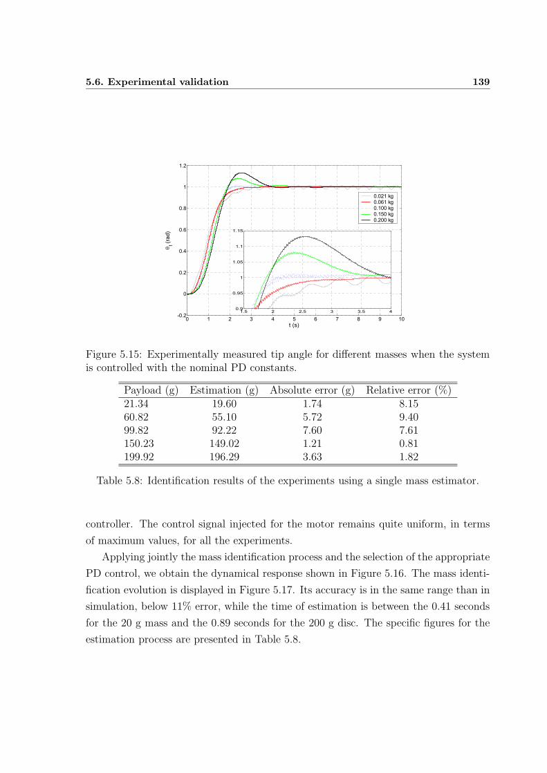
5.6. Experimental validation 139
0 1 2 3 4 5 6 7 8 9 10-0.2
0
0.2
0.4
0.6
0.8
1
1.2
t (s)
t (
rad)
0.021 kg0.061 kg0.100 kg0.150 kg0.200 kg
1.5 2 2.5 3 3.5 40.9
0.95
1
1.05
1.1
1.15
Figure 5.15: Experimentally measured tip angle for different masses when the systemis controlled with the nominal PD constants.
Payload (g) Estimation (g) Absolute error (g) Relative error (%)21.34 19.60 1.74 8.1560.82 55.10 5.72 9.4099.82 92.22 7.60 7.61150.23 149.02 1.21 0.81199.92 196.29 3.63 1.82
Table 5.8: Identification results of the experiments using a single mass estimator.
controller. The control signal injected for the motor remains quite uniform, in terms
of maximum values, for all the experiments.
Applying jointly the mass identification process and the selection of the appropriate
PD control, we obtain the dynamical response shown in Figure 5.16. The mass identi-
fication evolution is displayed in Figure 5.17. Its accuracy is in the same range than in
simulation, below 11% error, while the time of estimation is between the 0.41 seconds
for the 20 g mass and the 0.89 seconds for the 200 g disc. The specific figures for the
estimation process are presented in Table 5.8.
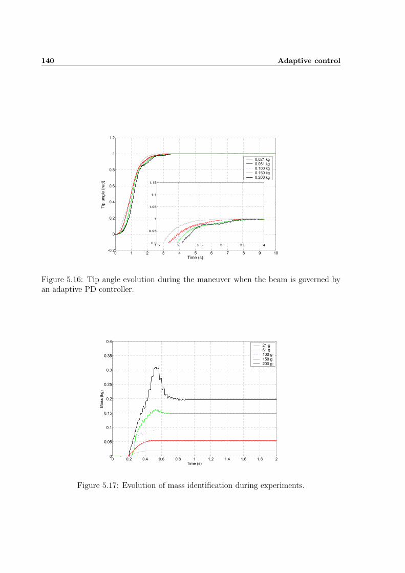
140 Adaptive control
0 1 2 3 4 5 6 7 8 9 10-0.2
0
0.2
0.4
0.6
0.8
1
1.2
Time (s)
Tip
angle
(ra
d)
0.021 kg0.061 kg0.100 kg0.150 kg0.200 kg
1.5 2 2.5 3 3.5 40.9
0.95
1
1.05
1.1
1.15
Figure 5.16: Tip angle evolution during the maneuver when the beam is governed byan adaptive PD controller.
0 0.2 0.4 0.6 0.8 1 1.2 1.4 1.6 1.8 20
0.05
0.1
0.15
0.2
0.25
0.3
0.35
0.4
Time (s)
Mass (
kg)
21 g61 g100 g150 g200 g
Figure 5.17: Evolution of mass identification during experiments.
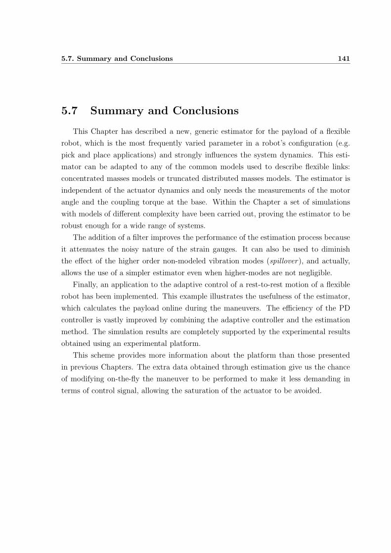
5.7. Summary and Conclusions 141
5.7 Summary and Conclusions
This Chapter has described a new, generic estimator for the payload of a flexible
robot, which is the most frequently varied parameter in a robot’s configuration (e.g.
pick and place applications) and strongly influences the system dynamics. This esti-
mator can be adapted to any of the common models used to describe flexible links:
concentrated masses models or truncated distributed masses models. The estimator is
independent of the actuator dynamics and only needs the measurements of the motor
angle and the coupling torque at the base. Within the Chapter a set of simulations
with models of different complexity have been carried out, proving the estimator to be
robust enough for a wide range of systems.
The addition of a filter improves the performance of the estimation process because
it attenuates the noisy nature of the strain gauges. It can also be used to diminish
the effect of the higher order non-modeled vibration modes (spillover), and actually,
allows the use of a simpler estimator even when higher-modes are not negligible.
Finally, an application to the adaptive control of a rest-to-rest motion of a flexible
robot has been implemented. This example illustrates the usefulness of the estimator,
which calculates the payload online during the maneuvers. The efficiency of the PD
controller is vastly improved by combining the adaptive controller and the estimation
method. The simulation results are completely supported by the experimental results
obtained using an experimental platform.
This scheme provides more information about the platform than those presented
in previous Chapters. The extra data obtained through estimation give us the chance
of modifying on-the-fly the maneuver to be performed to make it less demanding in
terms of control signal, allowing the saturation of the actuator to be avoided.

142 Adaptive control
Chapter 6
Wave-based control
6.1 Introduction
While the controllers presented in Chapters 4 and 5 achieve remarkable perfor-
mance when dealing with flexible systems, they are based on the assumption of small
displacements for the flexibility of the link. This hypothesis leads to a linear model
based on the simplification of the Euler-Bernouilli equation presented in (2.9). How-
ever, some emergent applications of flexible manipulators such as sensing devices (Ueno
et al., 1998) reject the linearity hypothesis, needing mathematical models that are able
to cope with large displacements appearing at the tip and the associated geometric
nonlinearities that this produces.
A model for this sort of extremely flexible manipulators (Payo et al., 2005) was
presented in Section 2.5, based on the non-linear spring behavior (duffing-like non-
linear differential equation). This topic has been briefly addressed in existing literature,
where, to the author’s knowledge only one other model (Lee, 2005) has been previously
defined (in fact, in the very same year).
Since the modeling has not yet been deeply studied yet, control of this kind of
structures is one of the topics still open in the field of flexible robotics, as mentioned
in Dr. Benosman’s survey (Benosman and LeVey, 2004). The present Chapter applies
one of the recent, innovative control strategies applied to control of elastic systems,
Wave-Based Control (WBC), to the control of manipulators that exhibit geometrical
non-linearities. Some drawbacks are found during application, but they can easily be
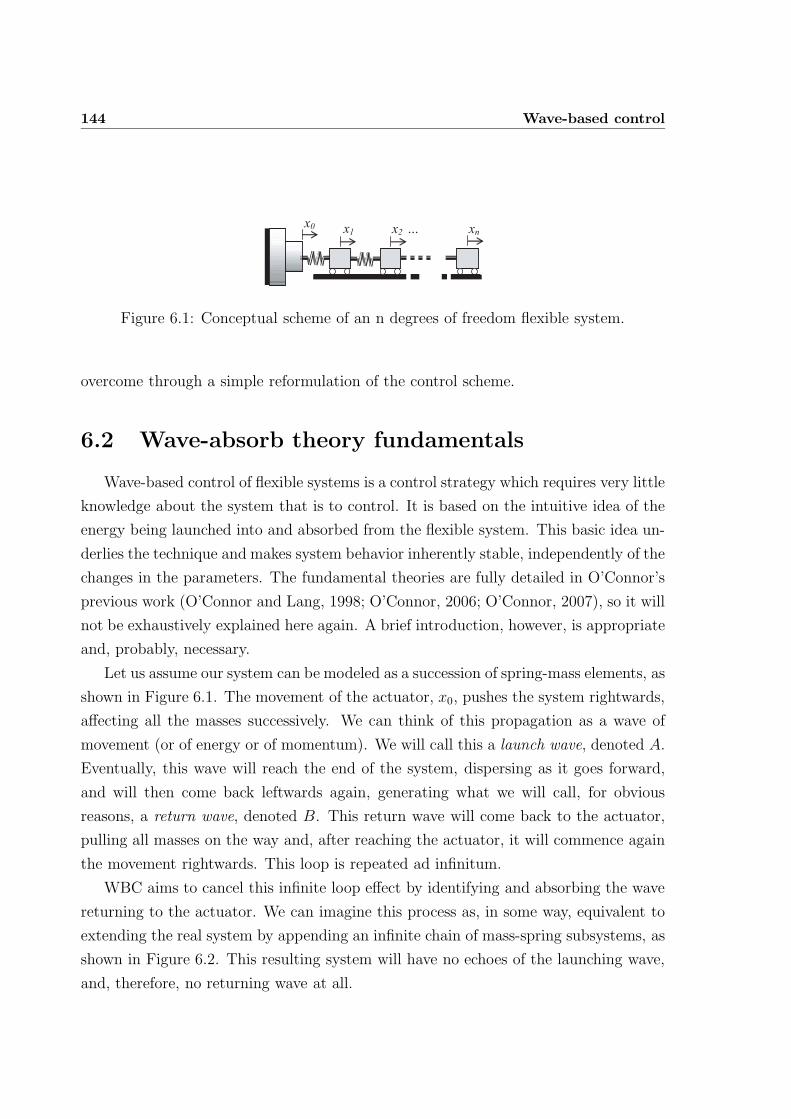
144 Wave-based control
x0 x1 xnx2 …
Figure 6.1: Conceptual scheme of an n degrees of freedom flexible system.
overcome through a simple reformulation of the control scheme.
6.2 Wave-absorb theory fundamentals
Wave-based control of flexible systems is a control strategy which requires very little
knowledge about the system that is to control. It is based on the intuitive idea of the
energy being launched into and absorbed from the flexible system. This basic idea un-
derlies the technique and makes system behavior inherently stable, independently of the
changes in the parameters. The fundamental theories are fully detailed in O’Connor’s
previous work (O’Connor and Lang, 1998; O’Connor, 2006; O’Connor, 2007), so it will
not be exhaustively explained here again. A brief introduction, however, is appropriate
and, probably, necessary.
Let us assume our system can be modeled as a succession of spring-mass elements, as
shown in Figure 6.1. The movement of the actuator, x0, pushes the system rightwards,
affecting all the masses successively. We can think of this propagation as a wave of
movement (or of energy or of momentum). We will call this a launch wave, denoted A.
Eventually, this wave will reach the end of the system, dispersing as it goes forward,
and will then come back leftwards again, generating what we will call, for obvious
reasons, a return wave, denoted B. This return wave will come back to the actuator,
pulling all masses on the way and, after reaching the actuator, it will commence again
the movement rightwards. This loop is repeated ad infinitum.
WBC aims to cancel this infinite loop effect by identifying and absorbing the wave
returning to the actuator. We can imagine this process as, in some way, equivalent to
extending the real system by appending an infinite chain of mass-spring subsystems, as
shown in Figure 6.2. This resulting system will have no echoes of the launching wave,
and, therefore, no returning wave at all.
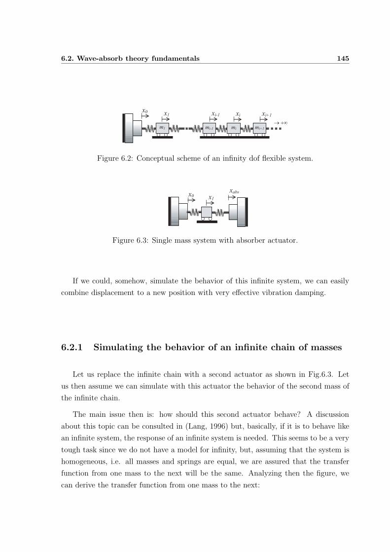
6.2. Wave-absorb theory fundamentals 145
x0 x1
m1 mi-1 mi mi+1
xi-1 xi xi+1
→ +∞
Figure 6.2: Conceptual scheme of an infinity dof flexible system.
x0 x1
xabs
Figure 6.3: Single mass system with absorber actuator.
If we could, somehow, simulate the behavior of this infinite system, we can easily
combine displacement to a new position with very effective vibration damping.
6.2.1 Simulating the behavior of an infinite chain of masses
Let us replace the infinite chain with a second actuator as shown in Fig.6.3. Let
us then assume we can simulate with this actuator the behavior of the second mass of
the infinite chain.
The main issue then is: how should this second actuator behave? A discussion
about this topic can be consulted in (Lang, 1996) but, basically, if it is to behave like
an infinite system, the response of an infinite system is needed. This seems to be a very
tough task since we do not have a model for infinity, but, assuming that the system is
homogeneous, i.e. all masses and springs are equal, we are assured that the transfer
function from one mass to the next will be the same. Analyzing then the figure, we
can derive the transfer function from one mass to the next:
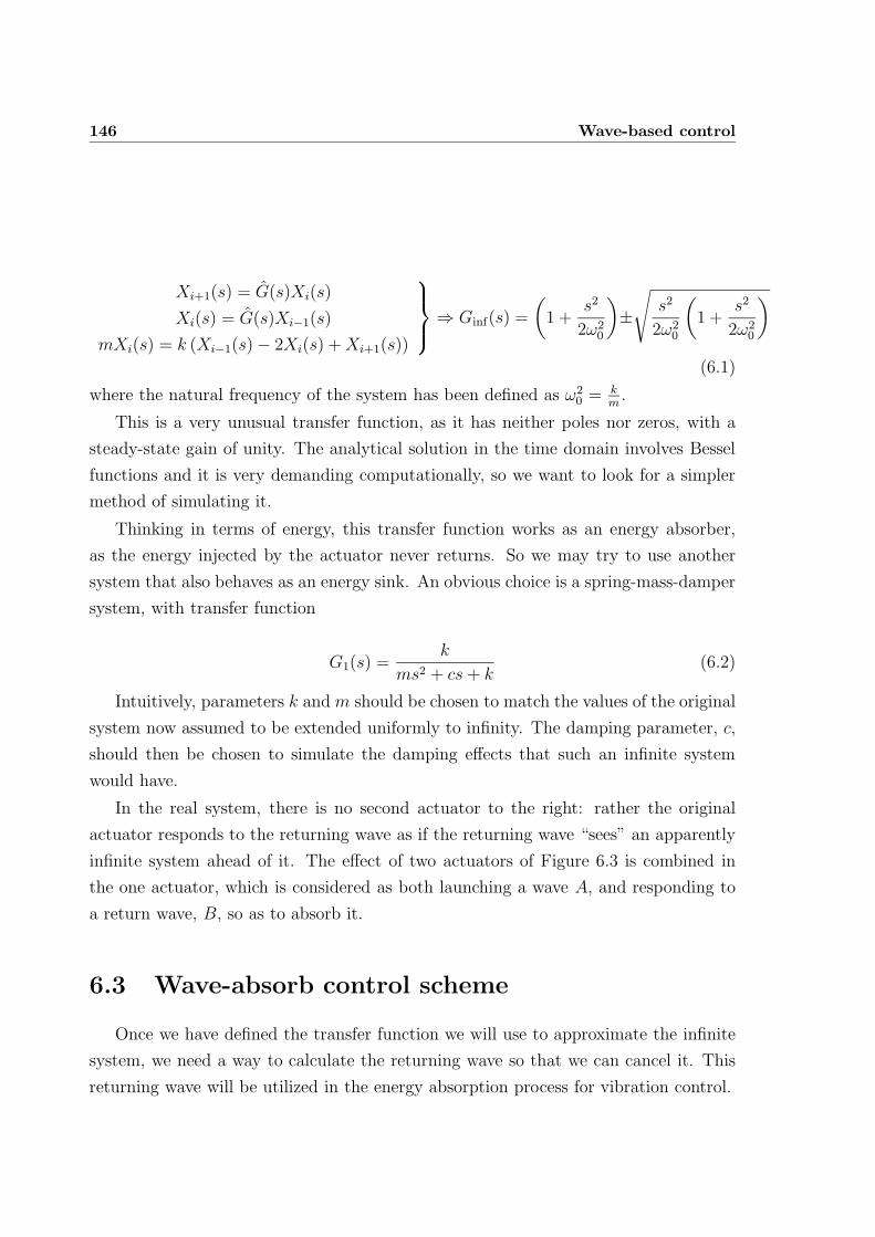
146 Wave-based control
Xi+1(s) = G(s)Xi(s)
Xi(s) = G(s)Xi−1(s)
mXi(s) = k (Xi−1(s)− 2Xi(s) +Xi+1(s))
⇒ Ginf(s) =
(
1 +s2
2ω20
)
±
√
s2
2ω20
(
1 +s2
2ω20
)
(6.1)
where the natural frequency of the system has been defined as ω20 = k
m.
This is a very unusual transfer function, as it has neither poles nor zeros, with a
steady-state gain of unity. The analytical solution in the time domain involves Bessel
functions and it is very demanding computationally, so we want to look for a simpler
method of simulating it.
Thinking in terms of energy, this transfer function works as an energy absorber,
as the energy injected by the actuator never returns. So we may try to use another
system that also behaves as an energy sink. An obvious choice is a spring-mass-damper
system, with transfer function
G1(s) =k
ms2 + cs+ k(6.2)
Intuitively, parameters k andm should be chosen to match the values of the original
system now assumed to be extended uniformly to infinity. The damping parameter, c,
should then be chosen to simulate the damping effects that such an infinite system
would have.
In the real system, there is no second actuator to the right: rather the original
actuator responds to the returning wave as if the returning wave “sees” an apparently
infinite system ahead of it. The effect of two actuators of Figure 6.3 is combined in
the one actuator, which is considered as both launching a wave A, and responding to
a return wave, B, so as to absorb it.
6.3 Wave-absorb control scheme
Once we have defined the transfer function we will use to approximate the infinite
system, we need a way to calculate the returning wave so that we can cancel it. This
returning wave will be utilized in the energy absorption process for vibration control.
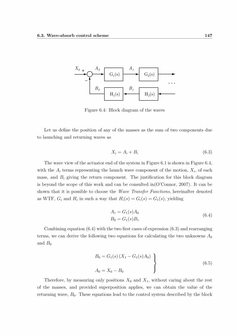
6.3. Wave-absorb control scheme 147
_
+G1(s)
H1(s) H2(s)
G2(s)
· · ·
X0
A0
A1
B0
B1
Figure 6.4: Block diagram of the waves
Let us define the position of any of the masses as the sum of two components due
to launching and returning waves as
Xi = Ai +Bi (6.3)
The wave view of the actuator end of the system in Figure 6.1 is shown in Figure 6.4,
with the Ai terms representing the launch wave component of the motion, Xi, of each
mass, and Bi giving the return component. The justification for this block diagram
is beyond the scope of this work and can be consulted in(O’Connor, 2007). It can be
shown that it is possible to choose the Wave Transfer Functions, hereinafter denoted
as WTF, Gi and Hi in such a way that Hi(s) = Gi(s) = G1(s), yielding
A1 = G1(s)A0
B0 = G1(s)B1
(6.4)
Combining equation (6.4) with the two first cases of expression (6.3) and rearranging
terms, we can derive the following two equations for calculating the two unknowns A0
and B0
B0 = G1(s) (X1 −G1(s)A0)
A0 = X0 −B0
(6.5)
Therefore, by measuring only positions X0 and X1, without caring about the rest
of the masses, and provided superposition applies, we can obtain the value of the
returning wave, B0. These equations lead to the control system described by the block
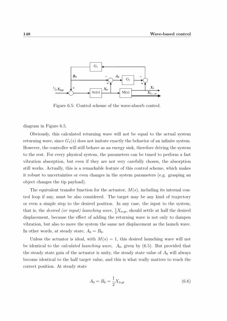
148 Wave-based control
Ac(s) M(s)
G1
G1
+ +
+1/2Xtrgt
_ _
X0X1
A0B0
X2,…,n
Figure 6.5: Control scheme of the wave-absorb control.
diagram in Figure 6.5.
Obviously, this calculated returning wave will not be equal to the actual system
returning wave, since G1(s) does not imitate exactly the behavior of an infinite system.
However, the controller will still behave as an energy sink, therefore driving the system
to the rest. For every physical system, the parameters can be tuned to perform a fast
vibration absorption, but even if they are not very carefully chosen, the absorption
still works. Actually, this is a remarkable feature of this control scheme, which makes
it robust to uncertainties or even changes in the system parameters (e.g. grasping an
object changes the tip payload).
The equivalent transfer function for the actuator, M(s), including its internal con-
trol loop if any, must be also considered. The target may be any kind of trajectory
or even a simple step to the desired position. In any case, the input to the system,
that is, the desired (or input) launching wave, 12Xtrgt, should settle at half the desired
displacement, because the effect of adding the returning wave is not only to dampen
vibration, but also to move the system the same net displacement as the launch wave.
In other words, at steady state, A0 = B0.
Unless the actuator is ideal, with M(s) = 1, this desired launching wave will not
be identical to the calculated launching wave, A0, given by (6.5). But provided that
the steady state gain of the actuator is unity, the steady state value of A0 will always
become identical to the half target value, and this is what really matters to reach the
correct position. At steady state
A0 = B0 =1
2Xtrgt (6.6)
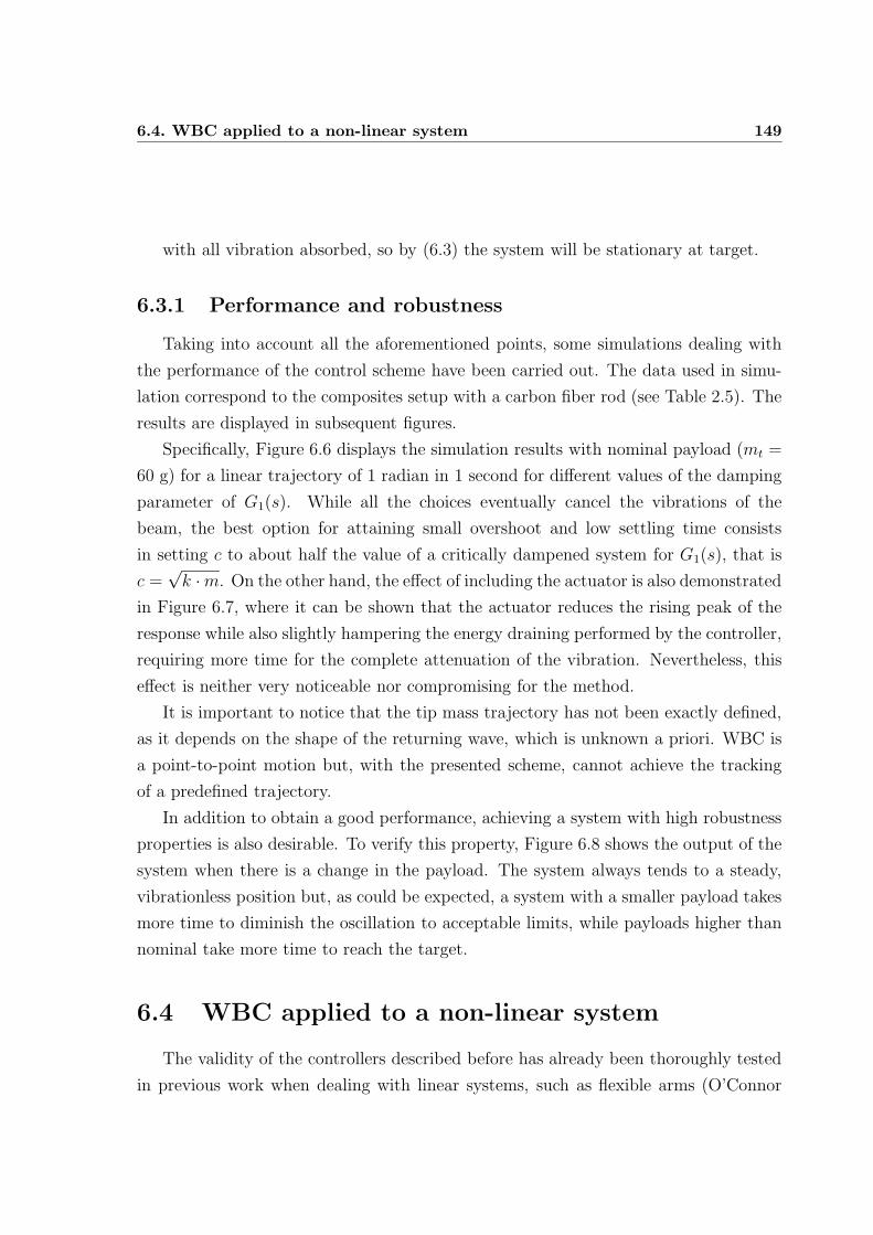
6.4. WBC applied to a non-linear system 149
with all vibration absorbed, so by (6.3) the system will be stationary at target.
6.3.1 Performance and robustness
Taking into account all the aforementioned points, some simulations dealing with
the performance of the control scheme have been carried out. The data used in simu-
lation correspond to the composites setup with a carbon fiber rod (see Table 2.5). The
results are displayed in subsequent figures.
Specifically, Figure 6.6 displays the simulation results with nominal payload (mt =
60 g) for a linear trajectory of 1 radian in 1 second for different values of the damping
parameter of G1(s). While all the choices eventually cancel the vibrations of the
beam, the best option for attaining small overshoot and low settling time consists
in setting c to about half the value of a critically dampened system for G1(s), that is
c =√k ·m. On the other hand, the effect of including the actuator is also demonstrated
in Figure 6.7, where it can be shown that the actuator reduces the rising peak of the
response while also slightly hampering the energy draining performed by the controller,
requiring more time for the complete attenuation of the vibration. Nevertheless, this
effect is neither very noticeable nor compromising for the method.
It is important to notice that the tip mass trajectory has not been exactly defined,
as it depends on the shape of the returning wave, which is unknown a priori. WBC is
a point-to-point motion but, with the presented scheme, cannot achieve the tracking
of a predefined trajectory.
In addition to obtain a good performance, achieving a system with high robustness
properties is also desirable. To verify this property, Figure 6.8 shows the output of the
system when there is a change in the payload. The system always tends to a steady,
vibrationless position but, as could be expected, a system with a smaller payload takes
more time to diminish the oscillation to acceptable limits, while payloads higher than
nominal take more time to reach the target.
6.4 WBC applied to a non-linear system
The validity of the controllers described before has already been thoroughly tested
in previous work when dealing with linear systems, such as flexible arms (O’Connor
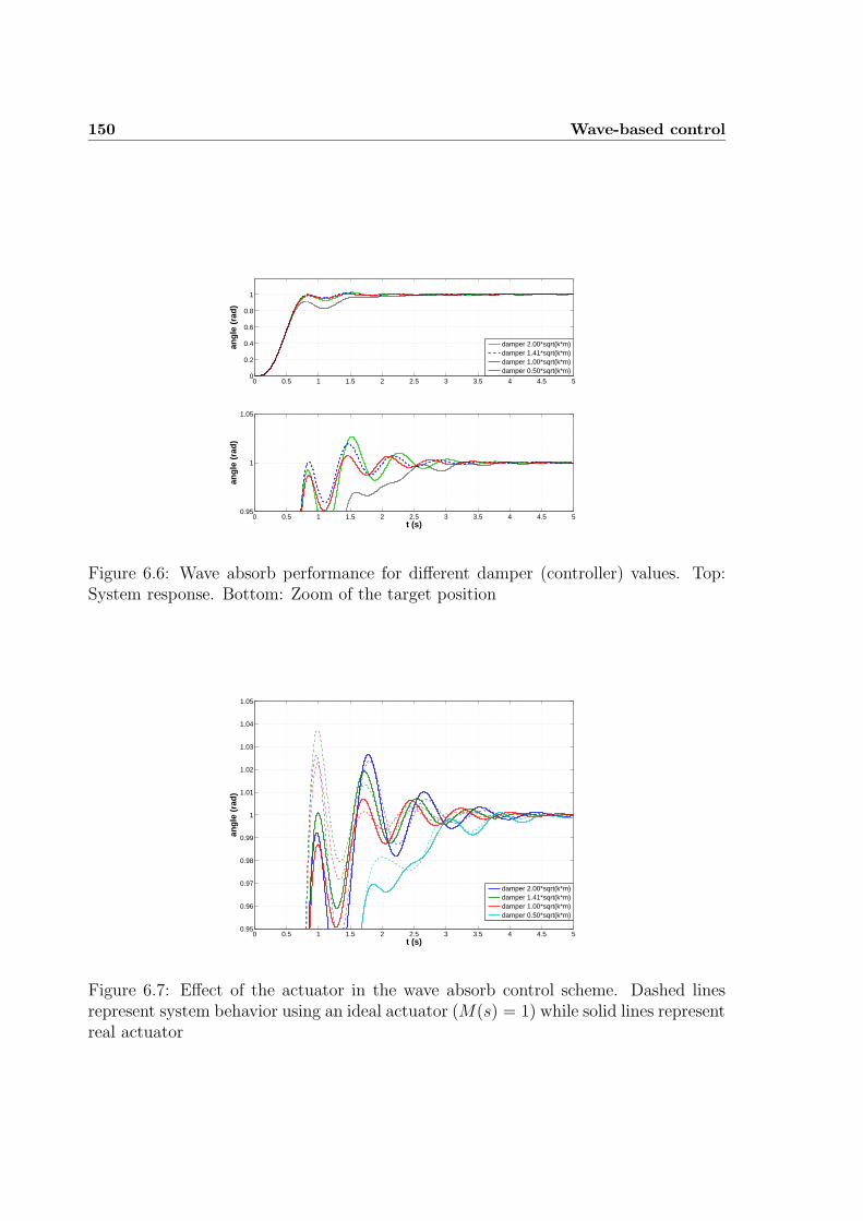
150 Wave-based control
0 0.5 1 1.5 2 2.5 3 3.5 4 4.5 50
0.2
0.4
0.6
0.8
1
angl
e (r
ad)
damper 2.00*sqrt(k*m)damper 1.41*sqrt(k*m)damper 1.00*sqrt(k*m)damper 0.50*sqrt(k*m)
0 0.5 1 1.5 2 2.5 3 3.5 4 4.5 50.95
1
1.05
angl
e (r
ad)
t (s)
Figure 6.6: Wave absorb performance for different damper (controller) values. Top:System response. Bottom: Zoom of the target position
0 0.5 1 1.5 2 2.5 3 3.5 4 4.5 50.95
0.96
0.97
0.98
0.99
1
1.01
1.02
1.03
1.04
1.05
angl
e (r
ad)
t (s)
damper 2.00*sqrt(k*m)damper 1.41*sqrt(k*m)damper 1.00*sqrt(k*m)damper 0.50*sqrt(k*m)
Figure 6.7: Effect of the actuator in the wave absorb control scheme. Dashed linesrepresent system behavior using an ideal actuator (M(s) = 1) while solid lines representreal actuator
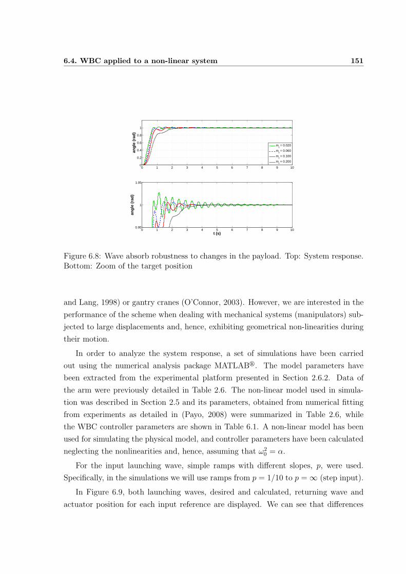
6.4. WBC applied to a non-linear system 151
0 1 2 3 4 5 6 7 8 9 100
0.2
0.4
0.6
0.8
1
angl
e (r
ad)
0 1 2 3 4 5 6 7 8 9 100.95
1
1.05
t (s)
angl
e (r
ad)
mt = 0.020
mt = 0.060
mt = 0.100
mt = 0.200
Figure 6.8: Wave absorb robustness to changes in the payload. Top: System response.Bottom: Zoom of the target position
and Lang, 1998) or gantry cranes (O’Connor, 2003). However, we are interested in the
performance of the scheme when dealing with mechanical systems (manipulators) sub-
jected to large displacements and, hence, exhibiting geometrical non-linearities during
their motion.
In order to analyze the system response, a set of simulations have been carried
out using the numerical analysis package MATLABr. The model parameters have
been extracted from the experimental platform presented in Section 2.6.2. Data of
the arm were previously detailed in Table 2.6. The non-linear model used in simula-
tion was described in Section 2.5 and its parameters, obtained from numerical fitting
from experiments as detailed in (Payo, 2008) were summarized in Table 2.6, while
the WBC controller parameters are shown in Table 6.1. A non-linear model has been
used for simulating the physical model, and controller parameters have been calculated
neglecting the nonlinearities and, hence, assuming that ω20 = α.
For the input launching wave, simple ramps with different slopes, p, were used.
Specifically, in the simulations we will use ramps from p = 1/10 to p = ∞ (step input).
In Figure 6.9, both launching waves, desired and calculated, returning wave and
actuator position for each input reference are displayed. We can see that differences
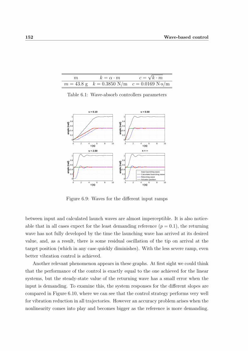
152 Wave-based control
m k = α ·m c =√k ·m
m = 43.8 g k = 0.3850 N/m c = 0.0169 N·s/m
Table 6.1: Wave-absorb controllers parameters
0 2 4 6 8 10
0
0.2
0.4
0.6
0.8
1
t (s)
angl
e (r
ad)
s = 0.10
0 2 4 6 8 10
0
0.2
0.4
0.6
0.8
1
t (s)
angl
e (r
ad)
s = 0.50
0 2 4 6 8 10
0
0.2
0.4
0.6
0.8
1
t (s)
angl
e (r
ad)
s = 2.50
0 2 4 6 8 10
0
0.2
0.4
0.6
0.8
1
t (s)
angl
e (r
ad)
s = ∞
Input launching waveCalculated launching waveReturning waveActuator position
Figure 6.9: Waves for the different input ramps
between input and calculated launch waves are almost imperceptible. It is also notice-
able that in all cases expect for the least demanding reference (p = 0.1), the returning
wave has not fully developed by the time the launching wave has arrived at its desired
value, and, as a result, there is some residual oscillation of the tip on arrival at the
target position (which in any case quickly diminishes). With the less severe ramp, even
better vibration control is achieved.
Another relevant phenomenon appears in these graphs. At first sight we could think
that the performance of the control is exactly equal to the one achieved for the linear
systems, but the steady-state value of the returning wave has a small error when the
input is demanding. To examine this, the system responses for the different slopes are
compared in Figure 6.10, where we can see that the control strategy performs very well
for vibration reduction in all trajectories. However an accuracy problem arises when the
nonlinearity comes into play and becomes bigger as the reference is more demanding.
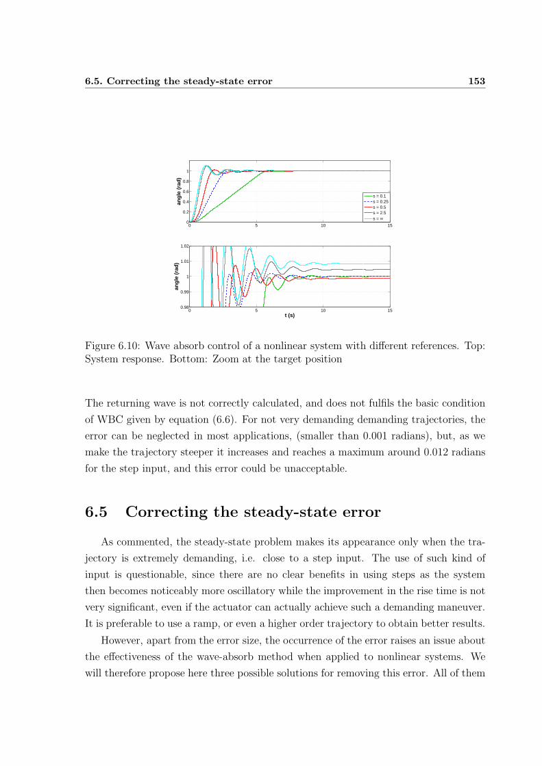
6.5. Correcting the steady-state error 153
0 5 10 150
0.2
0.4
0.6
0.8
1
angl
e (r
ad)
s = 0.1s = 0.25s = 0.5s = 2.5s = ∞
0 5 10 150.98
0.99
1
1.01
1.02
angl
e (r
ad)
t (s)
Figure 6.10: Wave absorb control of a nonlinear system with different references. Top:System response. Bottom: Zoom at the target position
The returning wave is not correctly calculated, and does not fulfils the basic condition
of WBC given by equation (6.6). For not very demanding demanding trajectories, the
error can be neglected in most applications, (smaller than 0.001 radians), but, as we
make the trajectory steeper it increases and reaches a maximum around 0.012 radians
for the step input, and this error could be unacceptable.
6.5 Correcting the steady-state error
As commented, the steady-state problem makes its appearance only when the tra-
jectory is extremely demanding, i.e. close to a step input. The use of such kind of
input is questionable, since there are no clear benefits in using steps as the system
then becomes noticeably more oscillatory while the improvement in the rise time is not
very significant, even if the actuator can actually achieve such a demanding maneuver.
It is preferable to use a ramp, or even a higher order trajectory to obtain better results.
However, apart from the error size, the occurrence of the error raises an issue about
the effectiveness of the wave-absorb method when applied to nonlinear systems. We
will therefore propose here three possible solutions for removing this error. All of them
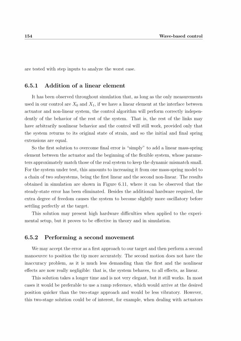
154 Wave-based control
are tested with step inputs to analyze the worst case.
6.5.1 Addition of a linear element
It has been observed throughout simulation that, as long as the only measurements
used in our control are X0 and X1, if we have a linear element at the interface between
actuator and non-linear system, the control algorithm will perform correctly indepen-
dently of the behavior of the rest of the system. That is, the rest of the links may
have arbitrarily nonlinear behavior and the control will still work, provided only that
the system returns to its original state of strain, and so the initial and final spring
extensions are equal.
So the first solution to overcome final error is “simply” to add a linear mass-spring
element between the actuator and the beginning of the flexible system, whose parame-
ters approximately match those of the real system to keep the dynamic mismatch small.
For the system under test, this amounts to increasing it from one mass-spring model to
a chain of two subsystems, being the first linear and the second non-linear. The results
obtained in simulation are shown in Figure 6.11, where it can be observed that the
steady-state error has been eliminated. Besides the additional hardware required, the
extra degree of freedom causes the system to become slightly more oscillatory before
settling perfectly at the target.
This solution may present high hardware difficulties when applied to the experi-
mental setup, but it proves to be effective in theory and in simulation.
6.5.2 Performing a second movement
We may accept the error as a first approach to our target and then perform a second
manoeuvre to position the tip more accurately. The second motion does not have the
inaccuracy problem, as it is much less demanding than the first and the nonlinear
effects are now really negligible: that is, the system behaves, to all effects, as linear.
This solution takes a longer time and is not very elegant, but it still works. In most
cases it would be preferable to use a ramp reference, which would arrive at the desired
position quicker than the two-stage approach and would be less vibratory. However,
this two-stage solution could be of interest, for example, when dealing with actuators
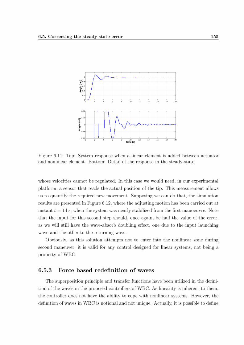
6.5. Correcting the steady-state error 155
0 2 4 6 8 10 12 14 16 18 200
0.2
0.4
0.6
0.8
1
Ang
le (
rad)
0 2 4 6 8 10 12 14 16 18 200.98
0.99
1
1.01
1.02
Time (s)
Ang
le (
rad)
Figure 6.11: Top: System response when a linear element is added between actuatorand nonlinear element. Bottom: Detail of the response in the steady-state
whose velocities cannot be regulated. In this case we would need, in our experimental
platform, a sensor that reads the actual position of the tip. This measurement allows
us to quantify the required new movement. Supposing we can do that, the simulation
results are presented in Figure 6.12, where the adjusting motion has been carried out at
instant t = 14 s, when the system was nearly stabilized from the first manoeuvre. Note
that the input for this second step should, once again, be half the value of the error,
as we will still have the wave-absorb doubling effect, one due to the input launching
wave and the other to the returning wave.
Obviously, as this solution attempts not to enter into the nonlinear zone during
second maneuver, it is valid for any control designed for linear systems, not being a
property of WBC.
6.5.3 Force based redefinition of waves
The superposition principle and transfer functions have been utilized in the defini-
tion of the waves in the proposed controllers of WBC. As linearity is inherent to them,
the controller does not have the ability to cope with nonlinear systems. However, the
definition of waves in WBC is notional and not unique. Actually, it is possible to define
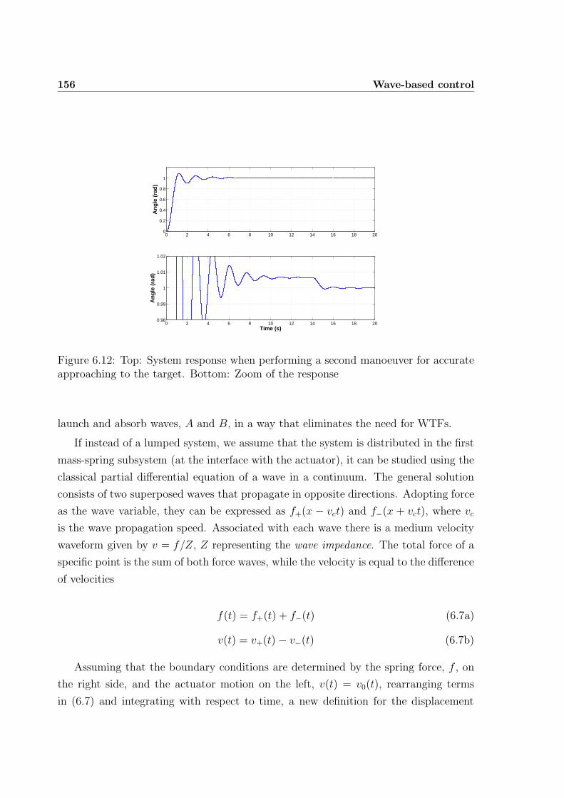
156 Wave-based control
0 2 4 6 8 10 12 14 16 18 200
0.2
0.4
0.6
0.8
1
Ang
le (
rad)
0 2 4 6 8 10 12 14 16 18 200.98
0.99
1
1.01
1.02
Time (s)
Ang
le (
rad)
Figure 6.12: Top: System response when performing a second manoeuver for accurateapproaching to the target. Bottom: Zoom of the response
launch and absorb waves, A and B, in a way that eliminates the need for WTFs.
If instead of a lumped system, we assume that the system is distributed in the first
mass-spring subsystem (at the interface with the actuator), it can be studied using the
classical partial differential equation of a wave in a continuum. The general solution
consists of two superposed waves that propagate in opposite directions. Adopting force
as the wave variable, they can be expressed as f+(x − vct) and f−(x + vct), where vc
is the wave propagation speed. Associated with each wave there is a medium velocity
waveform given by v = f/Z, Z representing the wave impedance. The total force of a
specific point is the sum of both force waves, while the velocity is equal to the difference
of velocities
f(t) = f+(t) + f−(t) (6.7a)
v(t) = v+(t)− v−(t) (6.7b)
Assuming that the boundary conditions are determined by the spring force, f , on
the right side, and the actuator motion on the left, v(t) = v0(t), rearranging terms
in (6.7) and integrating with respect to time, a new definition for the displacement
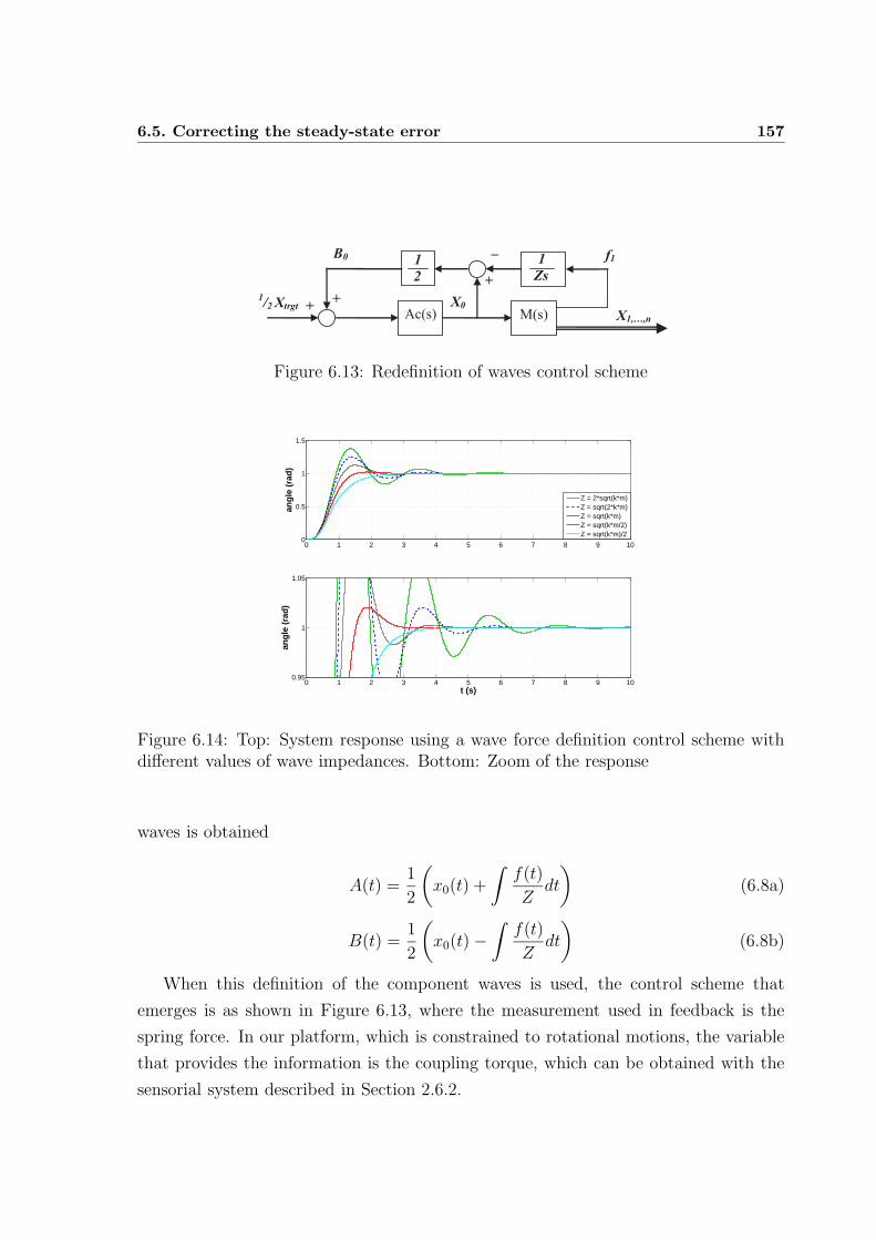
6.5. Correcting the steady-state error 157
Ac(s) M(s)
+
+1/2Xtrgt
_
X0
f1B0
X1,…,n
1
Zs
+
1
2
Figure 6.13: Redefinition of waves control scheme
0 1 2 3 4 5 6 7 8 9 100
0.5
1
1.5
angl
e (r
ad)
Z = 2*sqrt(k*m)Z = sqrt(2*k*m)Z = sqrt(k*m)Z = sqrt(k*m/2)Z = sqrt(k*m)/2
0 1 2 3 4 5 6 7 8 9 100.95
1
1.05
angl
e (r
ad)
t (s)
Figure 6.14: Top: System response using a wave force definition control scheme withdifferent values of wave impedances. Bottom: Zoom of the response
waves is obtained
A(t) =1
2
(
x0(t) +
∫f(t)
Zdt
)
(6.8a)
B(t) =1
2
(
x0(t)−∫
f(t)
Zdt
)
(6.8b)
When this definition of the component waves is used, the control scheme that
emerges is as shown in Figure 6.13, where the measurement used in feedback is the
spring force. In our platform, which is constrained to rotational motions, the variable
that provides the information is the coupling torque, which can be obtained with the
sensorial system described in Section 2.6.2.
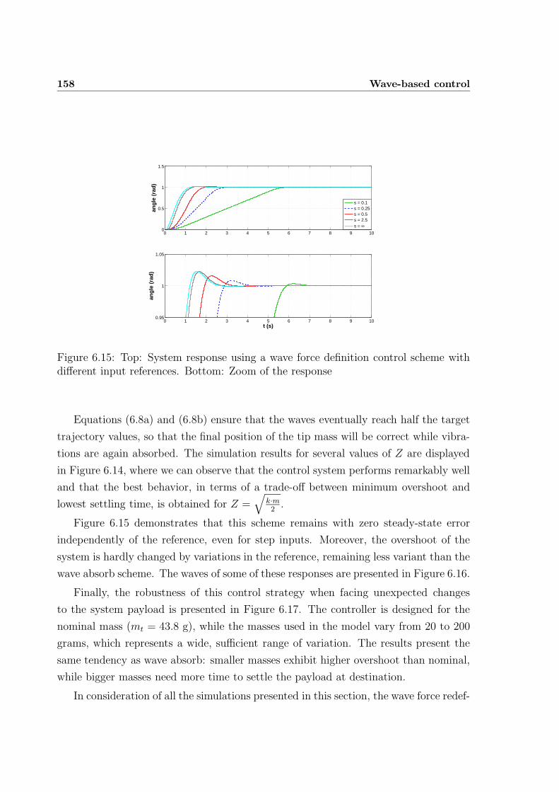
158 Wave-based control
0 1 2 3 4 5 6 7 8 9 100
0.5
1
1.5
angl
e (r
ad)
s = 0.1s = 0.25s = 0.5s = 2.5s = ∞
0 1 2 3 4 5 6 7 8 9 100.95
1
1.05
angl
e (r
ad)
t (s)
Figure 6.15: Top: System response using a wave force definition control scheme withdifferent input references. Bottom: Zoom of the response
Equations (6.8a) and (6.8b) ensure that the waves eventually reach half the target
trajectory values, so that the final position of the tip mass will be correct while vibra-
tions are again absorbed. The simulation results for several values of Z are displayed
in Figure 6.14, where we can observe that the control system performs remarkably well
and that the best behavior, in terms of a trade-off between minimum overshoot and
lowest settling time, is obtained for Z =√
k·m2.
Figure 6.15 demonstrates that this scheme remains with zero steady-state error
independently of the reference, even for step inputs. Moreover, the overshoot of the
system is hardly changed by variations in the reference, remaining less variant than the
wave absorb scheme. The waves of some of these responses are presented in Figure 6.16.
Finally, the robustness of this control strategy when facing unexpected changes
to the system payload is presented in Figure 6.17. The controller is designed for the
nominal mass (mt = 43.8 g), while the masses used in the model vary from 20 to 200
grams, which represents a wide, sufficient range of variation. The results present the
same tendency as wave absorb: smaller masses exhibit higher overshoot than nominal,
while bigger masses need more time to settle the payload at destination.
In consideration of all the simulations presented in this section, the wave force redef-
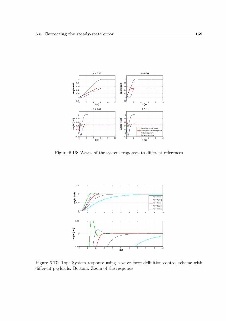
6.5. Correcting the steady-state error 159
0 2 4 6 8 10−0.2
0
0.2
0.4
0.6
0.8
1
t (s)
angl
e (r
ad)
s = 0.10
0 2 4 6 8 10−0.2
0
0.2
0.4
0.6
0.8
1
t (s)
angl
e (r
ad)
s = 0.50
0 2 4 6 8 10−0.2
0
0.2
0.4
0.6
0.8
1
t (s)
angl
e (r
ad)
s = 2.50
0 2 4 6 8 10−0.2
0
0.2
0.4
0.6
0.8
1
t (s)
angl
e (r
ad)
s = ∞
Input launching waveCalculated launching waveReturning waveActuator position
Figure 6.16: Waves of the system responses to different references
0 1 2 3 4 5 6 7 8 9 100
0.5
1
1.5
angl
e (r
ad)
mt = 20 g
mt = 43.8 g
mt = 60 g
mt = 100 g
mt = 200 g
0 1 2 3 4 5 6 7 8 9 100.95
1
1.05
angl
e (r
ad)
t (s)
Figure 6.17: Top: System response using a wave force definition control scheme withdifferent payloads. Bottom: Zoom of the response
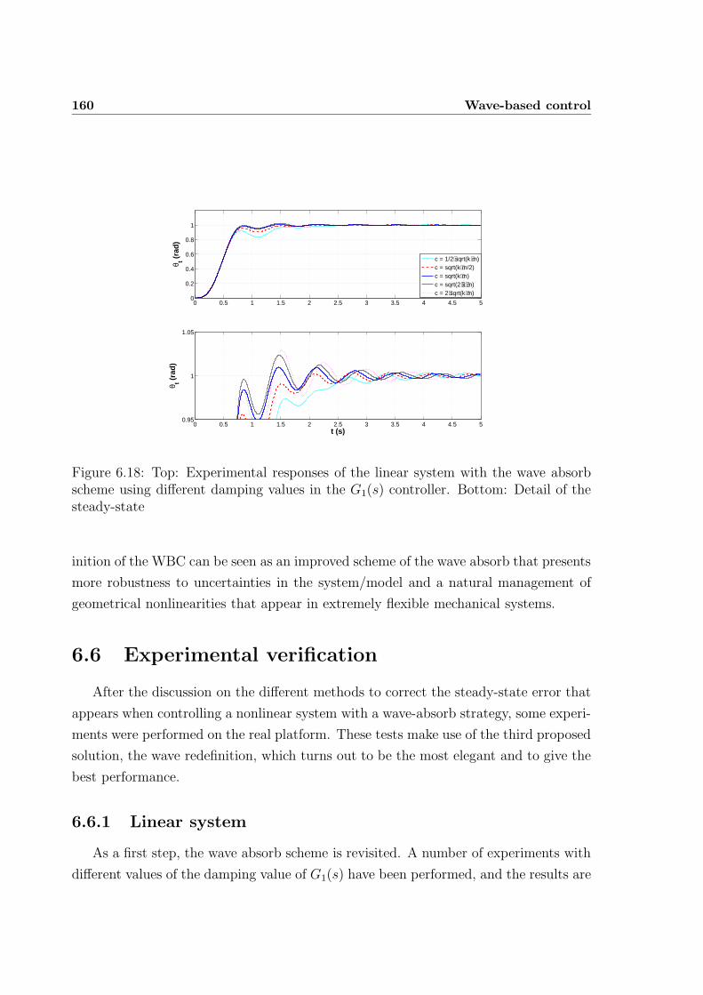
160 Wave-based control
0 0.5 1 1.5 2 2.5 3 3.5 4 4.5 50
0.2
0.4
0.6
0.8
1
θ t (ra
d)
0 0.5 1 1.5 2 2.5 3 3.5 4 4.5 50.95
1
1.05
θ t (ra
d)
t (s)
c = 1/2⋅sqrt(k⋅m)c = sqrt(k⋅m/2)c = sqrt(k⋅m)c = sqrt(2⋅k⋅m)c = 2⋅sqrt(k⋅m)
Figure 6.18: Top: Experimental responses of the linear system with the wave absorbscheme using different damping values in the G1(s) controller. Bottom: Detail of thesteady-state
inition of the WBC can be seen as an improved scheme of the wave absorb that presents
more robustness to uncertainties in the system/model and a natural management of
geometrical nonlinearities that appear in extremely flexible mechanical systems.
6.6 Experimental verification
After the discussion on the different methods to correct the steady-state error that
appears when controlling a nonlinear system with a wave-absorb strategy, some experi-
ments were performed on the real platform. These tests make use of the third proposed
solution, the wave redefinition, which turns out to be the most elegant and to give the
best performance.
6.6.1 Linear system
As a first step, the wave absorb scheme is revisited. A number of experiments with
different values of the damping value of G1(s) have been performed, and the results are
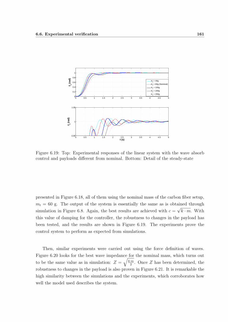
6.6. Experimental verification 161
0 0.5 1 1.5 2 2.5 3 3.5 4 4.5 50
0.2
0.4
0.6
0.8
1
θ t (ra
d)
0 0.5 1 1.5 2 2.5 3 3.5 4 4.5 50.95
1
1.05
θ t (ra
d)
t (s)
mt = 44g
mt = 60g (Nominal)
mt = 100g
mt = 150g
mt = 200g
Figure 6.19: Top: Experimental responses of the linear system with the wave absorbcontrol and payloads different from nominal. Bottom: Detail of the steady-state
presented in Figure 6.18, all of them using the nominal mass of the carbon fiber setup,
mt = 60 g. The output of the system is essentially the same as is obtained through
simulation in Figure 6.8. Again, the best results are achieved with c =√k ·m. With
this value of damping for the controller, the robustness to changes in the payload has
been tested, and the results are shown in Figure 6.19. The experiments prove the
control system to perform as expected from simulations.
Then, similar experiments were carried out using the force definition of waves.
Figure 6.20 looks for the best wave impedance for the nominal mass, which turns out
to be the same value as in simulation: Z =√
k·m2. Once Z has been determined, the
robustness to changes in the payload is also proven in Figure 6.21. It is remarkable the
high similarity between the simulations and the experiments, which corroborates how
well the model used describes the system.
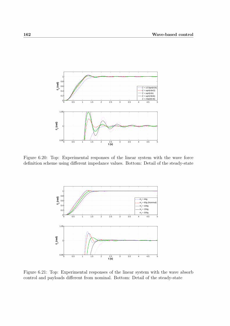
162 Wave-based control
0 0.5 1 1.5 2 2.5 3 3.5 4 4.5 50
0.2
0.4
0.6
0.8
1
θ t (ra
d)
0 0.5 1 1.5 2 2.5 3 3.5 4 4.5 50.95
1
1.05
θ t (ra
d)
t (s)
Z = 1/2⋅sqrt(k⋅m)Z = sqrt(k⋅m/2)Z = sqrt(k⋅m)Z = sqrt(2⋅k⋅m)Z = 2⋅sqrt(k⋅m)
Figure 6.20: Top: Experimental responses of the linear system with the wave forcedefinition scheme using different impedance values. Bottom: Detail of the steady-state
0 0.5 1 1.5 2 2.5 3 3.5 4 4.5 50
0.2
0.4
0.6
0.8
1
θ t (ra
d)
0 0.5 1 1.5 2 2.5 3 3.5 4 4.5 50.95
1
1.05
θ t (ra
d)
t (s)
mt = 44g
mt = 60g (Nominal)
mt = 100g
mt = 150g
mt = 200g
Figure 6.21: Top: Experimental responses of the linear system with the wave absorbcontrol and payloads different from nominal. Bottom: Detail of the steady-state
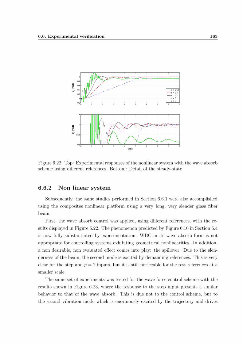
6.6. Experimental verification 163
0 1 2 3 4 5 6 7 8 9−0.2
0
0.2
0.4
0.6
0.8
1
θ t (ra
d)
0 1 2 3 4 5 6 7 8 90.9
0.95
1
1.05
θ t (ra
d)
t (s)
s = 1/10s = 1/4s = 1/2s = 2s = ∞
Figure 6.22: Top: Experimental responses of the nonlinear system with the wave absorbscheme using different references. Bottom: Detail of the steady-state
6.6.2 Non linear system
Subsequently, the same studies performed in Section 6.6.1 were also accomplished
using the composites nonlinear platform using a very long, very slender glass fiber
beam.
First, the wave absorb control was applied, using different references, with the re-
sults displayed in Figure 6.22. The phenomenon predicted by Figure 6.10 in Section 6.4
is now fully substantiated by experimentation: WBC in its wave absorb form is not
appropriate for controlling systems exhibiting geometrical nonlinearities. In addition,
a non desirable, non evaluated effect comes into play: the spillover. Due to the slen-
derness of the beam, the second mode is excited by demanding references. This is very
clear for the step and p = 2 inputs, but it is still noticeable for the rest references at a
smaller scale.
The same set of experiments was tested for the wave force control scheme with the
results shown in Figure 6.23, where the response to the step input presents a similar
behavior to that of the wave absorb. This is due not to the control scheme, but to
the second vibration mode which is enormously excited by the trajectory and drives
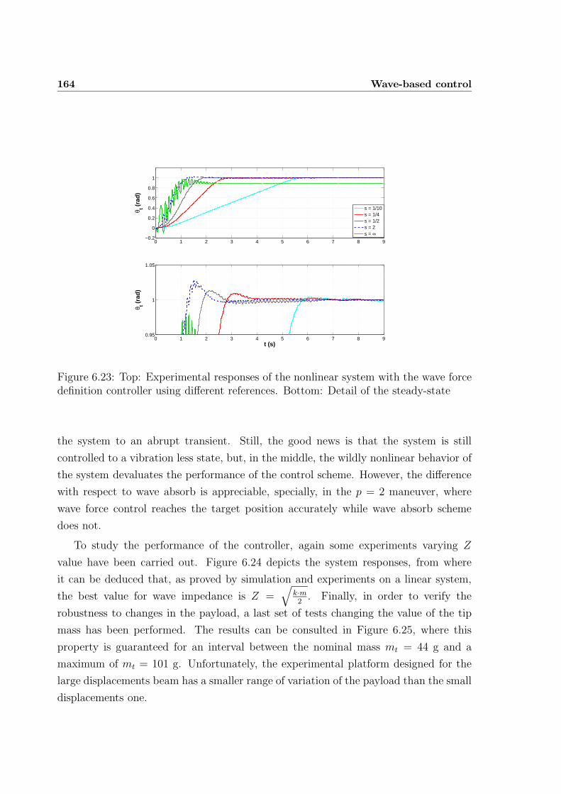
164 Wave-based control
0 1 2 3 4 5 6 7 8 9−0.2
0
0.2
0.4
0.6
0.8
1
θ t (ra
d)
0 1 2 3 4 5 6 7 8 90.95
1
1.05
θ t (ra
d)
t (s)
s = 1/10s = 1/4s = 1/2s = 2s = ∞
Figure 6.23: Top: Experimental responses of the nonlinear system with the wave forcedefinition controller using different references. Bottom: Detail of the steady-state
the system to an abrupt transient. Still, the good news is that the system is still
controlled to a vibration less state, but, in the middle, the wildly nonlinear behavior of
the system devaluates the performance of the control scheme. However, the difference
with respect to wave absorb is appreciable, specially, in the p = 2 maneuver, where
wave force control reaches the target position accurately while wave absorb scheme
does not.
To study the performance of the controller, again some experiments varying Z
value have been carried out. Figure 6.24 depicts the system responses, from where
it can be deduced that, as proved by simulation and experiments on a linear system,
the best value for wave impedance is Z =√
k·m2. Finally, in order to verify the
robustness to changes in the payload, a last set of tests changing the value of the tip
mass has been performed. The results can be consulted in Figure 6.25, where this
property is guaranteed for an interval between the nominal mass mt = 44 g and a
maximum of mt = 101 g. Unfortunately, the experimental platform designed for the
large displacements beam has a smaller range of variation of the payload than the small
displacements one.
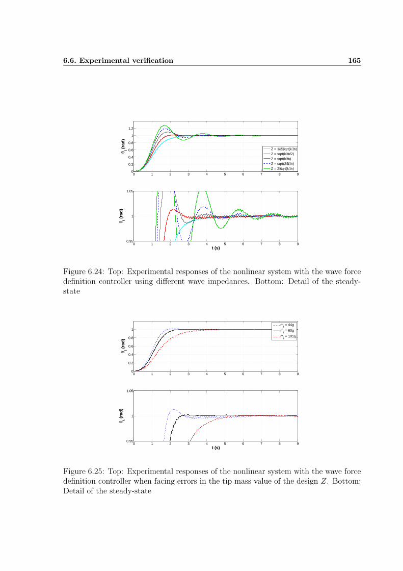
6.6. Experimental verification 165
0 1 2 3 4 5 6 7 8 90
0.2
0.4
0.6
0.8
1
1.2
θ t (ra
d)
0 1 2 3 4 5 6 7 8 90.95
1
1.05
θ t (ra
d)
t (s)
Z = 1/2⋅sqrt(k⋅m)Z = sqrt(k⋅m/2)Z = sqrt(k⋅m)Z = sqrt(2⋅k⋅m)Z = 2⋅sqrt(k⋅m)
Figure 6.24: Top: Experimental responses of the nonlinear system with the wave forcedefinition controller using different wave impedances. Bottom: Detail of the steady-state
0 1 2 3 4 5 6 7 8 90
0.2
0.4
0.6
0.8
1
θ t (ra
d)
0 1 2 3 4 5 6 7 8 90.95
1
1.05
θ t (ra
d)
t (s)
mt = 44g
mt = 60g
mt = 101g
Figure 6.25: Top: Experimental responses of the nonlinear system with the wave forcedefinition controller when facing errors in the tip mass value of the design Z. Bottom:Detail of the steady-state
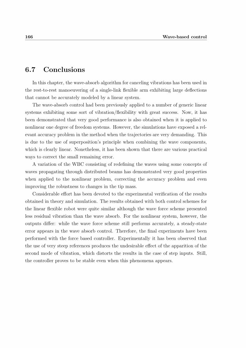
166 Wave-based control
6.7 Conclusions
In this chapter, the wave-absorb algorithm for canceling vibrations has been used in
the rest-to-rest manoeuvering of a single-link flexible arm exhibiting large deflections
that cannot be accurately modeled by a linear system.
The wave-absorb control had been previously applied to a number of generic linear
systems exhibiting some sort of vibration/flexibility with great success. Now, it has
been demonstrated that very good performance is also obtained when it is applied to
nonlinear one degree of freedom systems. However, the simulations have exposed a rel-
evant accuracy problem in the method when the trajectories are very demanding. This
is due to the use of superposition’s principle when combining the wave components,
which is clearly linear. Nonetheless, it has been shown that there are various practical
ways to correct the small remaining error.
A variation of the WBC consisting of redefining the waves using some concepts of
waves propagating through distributed beams has demonstrated very good properties
when applied to the nonlinear problem, correcting the accuracy problem and even
improving the robustness to changes in the tip mass.
Considerable effort has been devoted to the experimental verification of the results
obtained in theory and simulation. The results obtained with both control schemes for
the linear flexible robot were quite similar although the wave force scheme presented
less residual vibration than the wave absorb. For the nonlinear system, however, the
outputs differ: while the wave force scheme still performs accurately, a steady-state
error appears in the wave absorb control. Therefore, the final experiments have been
performed with the force based controller. Experimentally it has been observed that
the use of very steep references produces the undesirable effect of the apparition of the
second mode of vibration, which distorts the results in the case of step inputs. Still,
the controller proves to be stable even when this phenomena appears.
Chapter 7
Conclusions, contributions and
suggested future research
7.1 Summary and conclusions
Flexible robotics still has not reached its limit. While the modeling and position
control of these devices has been widely studied over the past three decades, the con-
tributions are in crescendo every year and new fields of application are continuously
reported and studied in literature. Recent advances in materials science, control theory,
sensors and actuators promote this sustained interest.
As commented in the Introduction, flexible robots provide a wonderful and motivat-
ing platform for corroborating the performance of innovative control techniques in a
simple, yet efficient, way. The present document deals with some of these schemes
(namely, dynamic inversion, robust and adaptive controls) and demonstrates their
properties with experimental results obtained from these arms.
Besides the study of novel control schemes for conventional flexible manipulators,
this Thesis raises the topic of controlling flexible links which are so slender that large
displacements can appear during maneuvers. The vibrationless point-to-point motion
of a flexible arm with these characteristics made of fiber glass has been properly ad-
dressed by means of a modification to the original wave-based control reported by Prof.
O’Connor. The models used for simulations purposes proved to be computationally
light while significantly more accurate than linear ones. The experimental results are
168 Conclusions, contributions and suggested future research
promising and there is scope for future developments. Some suggestions are enumerated
in Section 7.4were remarkably good.
7.2 Original contributions
Main contributions of the Thesis are listed below. Regarding control of robot links
subject to small displacements:
• Family of fourth-order, smooth polynomial trajectories that take into account
the physical limitations of the platform at the design stage.
• Direct dynamic inversion of the lumped masses model of a flexible link considered
in the Thesis.
• Control scheme robust to changes in the parameters of the plant (with stress on
payload changes) and to external perturbation for flexible robots.
• Adaptive control based in a novel payload estimation technique with application
to lumped and distributed masses models.
On the other hand, when dealing with extremely flexible robot arms (presenting
large displacements and geometrical non-linearities), the following topics have been
addressed:
• Application of wave-based control theory to control of manipulators whose links
are subject to large displacements, hence exhibiting geometrical nonlinear behav-
ior.
• Redefinition of the mechanical waves in a force-based manner to solve the preci-
sion issues of the wave-absorb schemes.
• Robustness to changes in the carried payload is inherent to the wave-based control
strategy, and it is a feature of both wave-absorb and force-based schemes.
7.3. List of publications 169
7.3 List of publications
The contents of this Thesis has given rise to the following articles published in
international journals with peer-reviewed selection processes:
• V. Feliu and F. Ramos, “Strain gauge based control of single-link very lightweight
flexible robots robust to payload changes”, Mechatronics, Volume 15, Issue 5,
June 2005, Pages 547-571. Impact factor: 1.434.
• F. Ramos, V. Feliu and I. Payo, “Design of trajectories with physical constraints
for very lightweight single-link flexible arms”, Journal of Vibration and Con-
trol, Volume 14, Issue 8, August 2008, Pages 1091-1110. Impact factor: 0.656.
• F. Ramos and V. Feliu, “New online payload identification for flexible robots.
Application to adaptive control”, Journal of Sound and Vibration, Volume
315, Issue 1-2, 5 August 2008, Pages 34-57. Impact factor: 1.364.
• W.J. O’Connor, F. Ramos, D.J. McKeown and V. Feliu, “Wave-based control
of non-linear flexible mechanical systems”, Nonlinear Dynamics, Volume 57,
Issue 1-2, July 2009, Pages 113-123. Impact factor: 1.295.
Also, the following communications were presented at international conferences with
peer-reviewed selection processes:
• I. Payo, F. Ramos, O.D. Cortazar and V. Feliu, Experimental validation of nonlin-
ear dynamic models for single-link very flexible arms, 44th IEEE Conference
on Decision and Control, published in Proceedings of the 44th IEEE
Conference on Decision and Control, and the European Control Con-
ference, CDC-ECC’05, Seville (Spain), December 2005.
• F. Ramos, V. Feliu and I. Payo, Design of trajectories with physical constraints for
very lightweight single link flexible arms, 8th Biennial ASME Conference
on Engineering Systems Design and Analysis, published in Proceedings
of 8th Biennial ASME Conference on Engineering Systems Design and
Analysis, ESDA2006, Torino (Italy), July 2006.
170 Conclusions, contributions and suggested future research
• W.J. OConnor, F. Ramos and V. Feliu, Wave-based control of a nonlinear flex-
ible system, 8th Biennial ASME Conference on Engineering Systems
Design and Analysis, published in Proceedings of 8th Biennial ASME
Conference on Engineering Systems Design and Analysis, ESDA2006,
Torino (Italy), July 2006.
• F. Ramos and W.J. O’Connor, Non-linear behavior in wave-based control, Amer-
ican Control Conference 2007, published in Proceedings of the Ameri-
can Control Conference 2007, ACC’07, New York (NY), July 2007.
Lastly, during the development of this Thesis some other works, related to the
control of flexible structures but non included in the contents of the Thesis, have
produced these further publications:
• F. Ramos, F.J. Castillo, J.A. Somolinos and V. Feliu, Control of a one degree-
of-freedom flexible arm with non neglected inertia at the payload, World Au-
tomation Congress 2004, published in Robotics: Trends, Principles,
and Applications - Proceedings of the 6th Biannual World Automation
Congress, Seville (Spain), June 2004.
• F. Ramos, I. Payo and V. Feliu, Comparativa entre dos esquemas de control
robusto de un robot flexible de un grado de libertad, XXV Jornadas de Au-
tomtica, Ciudad Real (Spain), September 2004.
• C.A. Monje, F. Ramos, V. Feliu and B.M. Vinagre, Tip position control of a
lightweight flexible manipulator using a fractional order controller, IET Control
Theory and Applications, Volume 1, Issue 5, September 2007, Pages 1451-
1460. Impact factor: 1.070.
• T.W. Yang, W.J. O’Connor and F. Ramos “Wave based slewing and vibration
control of a flexible arm”, International Journal of Intelligent Systems
Technologies and Applications, Volume 7, Issue 2, 2009, Pages 157-170. Im-
pact factor: Not Indexed.
7.4. Open topics for future research 171
7.4 Open topics for future research
This work presented a solution for the control of a single-link, very flexible robotic
manipulator. However, the study of these devices is at a very early stage for links
exhibiting geometric nonlinearities. Therefore, it is still necessary a great research
effort on the topic to find more generic solutions. Some of these future (not very far,
hopefully) contributions might be:
• Trajectory tracking of the very flexible manipulator.
• Modeling a two degrees-of-freedom manipulator made of composite materials.
Look for an extension to the multi-link case.
• Design and construction of this manipulator. To this end, a great effort should be
made in search of suitable actuators for driving the second very flexible link, as
they should be either as light as the composite links, if placed at the joint, or able
to transmit torque to the second link by means of a transmission mechanism such
as composites chains or a parallel kinematics mechanism in the line of (Somolinos
et al., 2002), if placed at the base. It is also highly convenient that sensorial
system be extremely light, for example a distributed optic fiber system (Payo
et al., 2009) could be appropriate.
• Design and construction of end-effector tools of adequate weight and dimensions
for the very flexible arm, e.g. a micro-gripper for grasping applications.
• More-in-depth study of the wave-based control applied to nonlinear systems con-
cerning issues such as the loss of performance when plant parameters vary.
• Dynamic inversion of the flexible link nonlinear model and design of a family of
trajectories specifically developed for the cancelation (or at least, reduction) of
vibration before control.
• Force control of flexible arms which exhibit large displacements of the link.
• Behavior when gravity is not compensated by an air table. This problem has
been addressed in the static case (Payo et al., 2004), while the dynamic has been
172 Conclusions, contributions and suggested future research
abandoned due to apparent randomness of the link movement when it has no
restrictions. A feasible approach might consist of providing some stiffness on
gravity axis preventing link bending in steady state. Might be with tendons-like
devices?
Bibliography
Abe, A. (2009). Trajectory planning for residual vibration suppression of a two-link
rigid-flexible manipulator considering large deformation. Mechanism and Machine
Theory, 44(9):1627–1639.
Al-Bedoor, B. O. and Hamdan, M. N. (2001). Geometrically non-linear dynamic model
of a rotating flexible arm. Journal of Sound and Vibration, 240(1):59–72.
Apkarian, P. and Adams, R. J. (1998). Advanced gain-scheduling techniques for un-
certain systems. IEEE Transactions on Control Systems Technology, 6(1):21–32.
Astrom, K. J. and Wittenmark, B. (1995). Adaptive Control. Addison Wesley, second
edition edition.
Balas, M. J. (1978a). Active control of flexible systems. Journal of Optimization,
Theory and Applications, 25(3):415–436.
Balas, M. J. (1978b). Feedback control of flexible systems. IEEE Transactions on
Automatic Control, 23(4):673–679.
Balas, M. J. (1979). Direct velocity feedback control of large space structures. Journal
of Guidance, Control, and Dynamics, 2(3):252–253.
Balas, M. J. (1982). Trends in large space structure control theory: fondest hopes,
wildest dreams. Journal of Guidance, Control, and Dynamics, 27(3):522–535.
Banavar, R. N. and Dominic, P. (1995). Lqg hinf controller for a flexible manipulator.
IEEE Transactions on Control Systems Technology, 3(4):409–416.
173
174 BIBLIOGRAPHY
Bayo, E. (1987). A finite-element approach to control the end-point motion of a single-
link flexible robot. Journal of Robotic Systems, 4(1):63–75.
Bayo, E. (1988). Computed torque for the position control of open-loop flexible robots.
In Proceedings of IEEE International Conference on Robotics and Automation,
pages 316–321.
Bayo, E. and Paden, B. (1987). On trajectory generation for flexible systems. Journal
of Robotic Systems, 4(2):229–235.
Baz, A., Imam, K., and McCoy, J. (1990). Active vibration control of flexible beams
using shape memory actuators. Journal of Sound and Vibration, 140(3):437–456.
Belendez, T., Neipp, C., and Belendez, A. (2002). Large and small deflections of a
cantilever beam. European Journal of Physics, 23(3):371–379.
Bellezza, F., Lanari, L., and Ulivi, G. (1990). Exact modeling of the flexible slewing
link. In Proceedings of the 1990 IEEE International Conference on Robotics and
Automation, volume 1, pages 734–739.
Benosman, A. and LeVey, G. (2004). Control of flexible manipulators: A survey.
Robotica, 22(5):533–545.
Berrocal, L. O. (2002). Resistencia de materiales. McGraw Hill, 2 edition.
Book, W. J. (1974). Modeling, design and control of flexible manipulator arms. PhD
thesis, Massachusetts Institute of Technology, Dept. of Mechanical Engineering.
Book, W. J. (1984). Recursive lagrangian dynamics for flexible manipulator arms.
International Journal of Robotics Research, 3(3):87–101.
Book, W. J. (1993). Controlled motion in an elastic world. Journal of Dynamic
Systems, Measurement and Control, Transactions of the ASME, 115(2 B):252–
261.
Book, W. J., Maizza-Neto., O., and Whitney, D. E. (1975). Feedback control of two
beam, two joint systems with distributed flexibility. Journal of Dynamic Systems,
Measurement and Control, Transactions of the ASME, 97 Ser G(4):424–431.
BIBLIOGRAPHY 175
Book, W. J. and Majette, M. (1983). Controller design for flexible, distributed pa-
rameter mechanical arms via combined state space and frequency domain tech-
niques. Journal of Dynamic Systems, Measurement and Control, Transactions of
the ASME, 105(4):245–254.
Boyer, F. and Coiffet, P. (1996). Generalization of newton-euler model for flexible
manipulators. Journal of Robotic Systems, 13(1):11–24.
Brockett, R. W. and Mesarovic, M. D. (1965). The reproducibility of multivariable
control systems. Journal of Mathematical Analysis and Applications, pages 548–
563.
Cannon, R. H. and Schmitz, E. (1984). Initial experiments on the end-point control of
a flexible one-link robot. The International Journal of Robotics Research, 3(3):62–
75.
Chalhoub, N. G., Kfoury, G. A., and Bazzi, B. A. (2006). Design of robust controllers
and a nonlinear observer for the control of a single-link flexible robotic manipula-
tor. Journal of Sound and Vibration, 291(1-2):437–461.
Choi, S. B. and Cheong, C. (1996). Vibration control of a flexible beam using shape
memory alloy actuators. Journal of Guidance, Control, and Dynamics, 19(5):1178–
1180.
Choi, S. B., Cheong, C. C., Thompson, B. S., and Gandhi, M. V. (1994). Vibration
control of flexible linkage mechanisms using piezoelectric films. Mechanism and
Machine Theory, 29(4):535–546.
Choi, S. B., Park, Y. K., and Cheong, C. C. (1996). Active vibration control of
intelligent composite laminate structures incorporating an electro-rheological fluid.
Journal of Intelligent Material Systems and Structures, 7(4):411–419.
Choi, S. B., Thompson, B. S., and Gandhi, M. V. (1995). Control of a single-link flexible
manipulator fabricated from composite laminates. Journal of Robotic Systems,
12(1):45–54.
176 BIBLIOGRAPHY
Christoforou, E. G. and Damaren, C. J. (2000). The control of flexible-link robots ma-
nipulating large payloads: Theory and experiments. Journal of Robotic Systems,
17(5):255–271.
Clough, R. and Penzien, J. (1993). Dynamics of structures. Mc Graw-Hill.
Damaren, C. and Sharf, I. (1995). Simulation of flexible-link manipulators with inertial
and geometric nonlinearities. Journal of Dynamic Systems, Measurement and
Control, Transactions of the ASME, 117(1):74–87.
Damaren, C. J. (1996). Adaptive control of flexible manipulators carrying large uncer-
tain payloads. Journal of Robotic Systems, 13(4):219–228.
DeLuca, A. and Siciliano, B. (1989). Trajectory control of a non-linear one-link flexible
arm. International Journal of Control, 50(5):1699–1715.
DeLuca, A. and Siciliano, B. (1991). Closed-form dynamic-model of planar multi-
link lightweight robots. IEEE Transactions on Systems, Man and Cybernetics,
21(4):826–839.
DeLuca, A. and Siciliano, B. (1993). Regulation of flexible arms under gravity. IEEE
Transactions on Robotics and Automation, 9(4):463–467.
Denavit, J. and Hartenberg, R. (1955). A kinematic notation for lower-pair mechanisms
based on matrices. ASME Journal of Applied Mechanics, pages 215–221.
Devasia, S. and Paden, B. (1994). Exact output tracking for nonlinear time-varying
systems. pages 2346–2355, Lake Buena Vista, CA.
Dıaz, I. M. (2007). Desarrollo, modelado e instrumentacion de estructuras flexibles
para la cancelacion activa de vibraciones. PhD thesis, Escuela Tecnica Superior de
Ingenieros Industriales, Universidad de Castilla-La Mancha, Ciudad Real, Spain.
Dwivedy, S. K. and Eberhard, P. (2006). Dynamic analysis of flexible manipulators, a
literature review. Mechanism and Machine Theory, 41(7):749–777.
Fattah, A., Angeles, J., and Misra, A. K. (1995). Dynamics of a 3-dof spatial parallel
manipulator with flexible links. volume 1, pages 627–632.
BIBLIOGRAPHY 177
Feliu, J. J. (1997). Desarrollo de Modelos Dinamicos Computacionalmente Eficientes
para Robots Flexibles de Un Grado de Libertad. Aplicacion al Control Adaptativo.
PhD thesis, National University of University Distance Learning.
Feliu, J. J., Feliu, V., and Cerrada, C. (1999). Load adaptive control of single-link
flexible arms based on a new modeling technique. IEEE Transactions on Robotics
and Automation, 15(5):793–804.
Feliu, V. (2006). Robots flexibles: hacia una generacin de robots con nuevas presta-
ciones. Revista Iberoamericana de Automtica e Informtica Industrial, 3(3):24–41.
Feliu, V. and Ramos, F. (2005). Strain gauge based control of single-link very
lightweight flexible robots robust to payload changes. Mechatronics, 15(5):547–
571.
Feliu, V., Rattan, K., and Jr., H. B. (1991). Modelling and control of single-link flexible
arms with lumped masses. ASME Journal of Dynamic Systems, Measurements
and Control, 114:59–69.
Feliu, V. and Rattan, K. S. (1999). Feedforward control of single-link flexible manipu-
lators by discrete model inversion. Journal of Dynamic Systems Measurement and
Control-Transactions of the ASME, 121(4):713–721.
Feliu, V., Rattan, K. S., and Brown, H. B. (1990). Adaptative control of a single-link
flexible manipulator. IEEE Control Systems Magazine, 10(2):29–33.
Feliu, V., Rattan, K. S., and Brown, H. B. (1992). Modeling and control of single-link
flexible arms with lumped masses. Journal of Dynamic Systems, Measurement
and Control, 114(3):59–69.
Feliu, V., Rattan, K. S., and Brown, H. B. (1993). Control of flexible arms with friction
in the joints. IEEE Transactions on Robotics and Automation, 9(4):467–475.
Feliu, V., Somolinos, J. A., Cerrada, C., and Cerrada, J. A. (1997). A new control
scheme of single-link flexible manipulators robust to payload changes. Journal of
Intelligent and Robotic Systems, 20(2-4):349–373.
178 BIBLIOGRAPHY
Feliu, V., Somolinos, J. A., and Garcıa, A. (2003). Inverse dynamics based control
system for a three-degree-of-freedom flexible arm. IEEE Transactions on Robotics
and Automation, 19(6):1007–1014.
Feliu, V., Somolinos, J. A., Garcıa, A., and Sanchez, L. (2002). Robustness comparative
study of two control schemes for 3-dof flexible manipulators. Journal of Intelligent
and Robotic Systems, 34(4):467–488.
Garcıa, A. (1999). Control combinado posicion/fuerza de un robot con dos eslabones
flexibles y tres grados de libertad. PhD thesis, Universidad Politecnica de Madrid.
Garcıa, A. and Feliu, V. (2000). Force control of a single-link flexible robot based on a
collision detection mechanism. IEE Proceedings: Control Theory and Applications,
147(6):588–595.
Garcıa, A., Feliu, V., and Somolinos, J. A. (2003). Experimental testing of a gauge
based collision detection mechanism for a new three-degree-of-freedom flexible
robot. Journal of Robotic Systems, 20(6):271–284.
Ge, S. S., Lee, T. H., and Zhu, G. (1996). Energy-based robust controller design for
multi-link flexible robots. Mechatronics, 6(7):779–798.
Ge, S. S., Lee, T. H., and Zhu, G. (1998). Improving regulation of a single-link flexible
manipulator with strain feedback. IEEE Transactions on Robotics and Automa-
tion, 14(1):179–185.
Gu, M. and Piedboeuf, J.-C. (2003). A flexible-arm as manipulator position and force
detection unit. Control Engineering Practice, 11:1433–1448.
Gutierrez, L. B., Lewis, F. L., and Lowe, J. A. (1998). Implementation of a neural
network tracking controller for a single flexible link: Comparison with pd and pid
controllers. IEEE Transactions on Industrial Electronics, 45(2):307–318.
Halim, D. and Moheimani, S. O. R. (2002a). Experimental implementation of spatial
hinf control on a piezoelectric laminated beam. IEEE/ASME Transactions on
Mechatronics, 7(3):346–356.
BIBLIOGRAPHY 179
Halim, D. and Moheimani, S. O. R. (2002b). Spatial h2 control of a piezoelectric
laminate beam: experimental implementation. IEEE Transactions on Control
Systems Technology, 10(4):533–546.
Harris, C. and Miles, J. (1975). Adaptive control of nonlinear flexible spacecraft. In
Proceedings of the IFAC 6th World Conference, Boston, MA.
Hastings, G. G. (1986). Controlling flexible manipulators, an experimental investiga-
tion. PhD thesis, Georgia Institute of Technology.
Hastings, G. G. and Book, W. J. (1987). Linear dynamic model for flexible robotic
manipulators. IEEE Control Systems Magazine, 7(1):61–64.
Hu, C. M. (2005). Wave-Based Control of Elastic Mechanical Systems. PhD thesis,
UCD, National University of Ireland.
Karimi, H. R., Yazdanpanah, M. J., Patel, R. V., and Khorasani, K. (2006). Modeling
and control of linear two-time scale systems: Applied to single-link flexible ma-
nipulator. Journal of Intelligent and Robotic Systems: Theory and Applications,
45(3):235–265.
Karkoub, M. and Tamma, K. (2001). Modelling and µ-synthesis control of flexible
manipulators. Computers and Structures, 79(5):543–551.
Kitagawa, H., Beppu, T., Kobayashi, T., and Terashima, K. (2002). Motion control
of omnidirectional wheelchair considering patient comfort. In Proceedings of the
IFAC World Congress, Barcelona, Spain.
Koehne, M. (1971). Optimal feedback control of flexible mechanical systems. In Pro-
ceedings of the IFAC Symposium on the Optimal Control of Distributed Parameter
Systems, Banff, Canada.
Koivo, A. and Lee, K. (1989). Self-tuning control of planar two-link manipulator
with nonrigid arms. In Proceedings of the 1989 IEEE International Conference on
Robotics and Automation, page 10301035, Scottdale.
180 BIBLIOGRAPHY
Komkov, V. (1968). Optimal control of a transverse vibration of a beam. SIAM Journal
on Control, 6(3):401.
Landau, L. and Lifshitz, E. (1969). Theory of Elasticity. Editorial Reverte S.A.
Lang, D. (1996). Development of an Adaptive Control Strategy for Elastic Mechanical
Systems. PhD thesis, UCD, National University of Ireland.
Larson, V. and Likins, P. (1976). An application of modern control theory to an elastic
spacecraft. In ESA Symposium on Dynamics and Control of Non-Rigid Space
Vehicles, Frascati, Italy.
Lee, H. H. (2005). New dynamic modeling of flexible-link robots. Journal of Dynamic
Systems Measurement and Control-Transactions of the ASME, 127(2):307–309.
Lee, K. (2002). Large deflections of cantilever beams of non-linear elastic material under
a combined loading. International Journal of Non-Linear Mechanics, 37:439–443.
Lee, K., Wilson, J., and Oh, S. (1993). Elastica of cantilevered beams with variable
cross section. International Journal of Non-Linear Mechanics, 28(5):579–589.
Lee, T. H., Ge, S. S., and Wang, Z. P. (2001). Adaptive robust controller design for
multi-link flexible robots. Mechatronics, 11(8):951–967.
Lin, J. and Lewis, F. L. (2002). Fuzzy controller for flexible-link robot arm by reduced-
order techniques. IEE Proceedings: Control Theory and Applications, 149(3):177–
187.
Lin, Y. J. and Lee, T. S. (1993). An investigation of fuzzy-logic control of flexible
robots. Robotica, 11(4):363–371.
Luo, Z.-H. (1993). Direct strain feedback control of flexible robot arms: new theoretical
and experimental results. IEEE Transactions on Automatic Control, 38(11):1610–
1622.
Maizza-Neto, O. (1974). Modal analysis and control of flexible manipulator arms. PhD
thesis, Massachusetts Institute of Technology, Dept. of Mechanical Engineering.
BIBLIOGRAPHY 181
Marro, G. and Piazzi, A. (1996). A geometric approach to multivariable perfect track-
ing. In Proceedings of the IFAC 13th World Conference, pages 241–246, San Fran-
cisco, CA.
Meckl, P. H. (1988). Control of Vibration in Mechanical Systems Using Shaped Ref-
erence Inputs. PhD thesis, The Artifical Intelligence Laboratory, Massachusetts
Institute of Technology.
Meckl, P. H. and Seering, W. P. (1985). Minimizing residual vibration for point-to-
point motion. Journal of vibration, acoustics, stress, and reliability in design,
107(4):378–382.
Meirovitch, L. (1997). Principles and Techniques of Vibrations. Prentice-Hall, New
Jersey.
Meirovitch, L., VanLandingham, H., and Oz, H. (1977). Control of spinning flexible
spacecraft by modal synthesis. Acta Astronautica, 4(9-10):985–1010.
Mirro, J. (1972). Automatic feedback control of a vibrating flexible beam. Master’s
thesis, Massachusetts Institute of Technology, Dept. of Mechanical Engineering.
Mohamed, Z., Chee, A. K., Hashim, A. W. I. M., Tokhi, M. O., Amin, S. H. M., and
Mamat, R. (2006). Techniques for vibration control of a flexible robot. Robotica,
24(4):499–511.
Moudgal, V. G., Kwong, W. A., Passino, K. M., and Yurkovich, S. (1995). Fuzzy
learning control for a flexible-link robot. IEEE Transactions on Fuzzy Systems,
3(2):199–210.
Nicosia, S., Tomei, P., and Tornambe, A. (1986). Dynamic modelling of flexible
robot manipulators. In Proceedings of the 1986 IEEE International Conference
on Robotics and Automation, volume 3, pages 365–372.
Oakley, C. M. and Cannon, R. H. (1988a). End-point control of a two-link manipu-
lator with a very flexible forearm: issues and experiments. In Proceedings of the
American Control Conference, pages 1381–1388.
182 BIBLIOGRAPHY
Oakley, C. M. and Cannon, R. H. (1988b). Initial experiments on the control of a
two-link flexible manipulator with a very flexible forearm. In Proceedings of the
American Control Conference, pages 996–1002.
Oakley, C. M. and Cannon, R. H. (1990). Anatomy of an experimental two-link flexible
manipulator under end-point control. In Proceedings of the IEEE Conference on
Decision and Control, volume 2, pages 507–513.
O’Connor, W. (2003). A gantry crane problem solved. Journal of Dynamic Systems
Measurement and Control-Transactions of the ASME, 125(4):569–576.
O’Connor, W. J. (2006). Wave-echo control of lumped flexible systems. Journal of
Sound and Vibration, 298(4-5):1001–1018.
O’Connor, W. J. (2007). Wave-based analysis and control of lump-modeled flexible
robots. IEEE Transactions on Robotics, 23(2):342–352.
O’Connor, W. J. and Lang, D. (1998). Position control of flexible robot arms us-
ing mechanical waves. Journal of Dynamic Systems Measurement and Control-
Transactions of the Asme, 120(3):334–339.
Ogata, K. (2001). Modern Control Engineering. Prentice Hall, 4th edition.
Paganini, F. and Feron, E. (1999). Recent advances on LMI methods in control, chapter
LMI methods for robust H2 analysis: A survey with comparisons. SIAM.
Pao, L. Y. (1999). Multi-input shaping design for vibration reduction. Automatica,
35(1):81–89.
Payo, I. (2008). Aportaciones al control de robots flexibles ligeros de un grado de libertad
fabricados con material compuesto mediante sensores extensometricos. PhD thesis,
Escuela Tecnica Superior de Ingenieros Industriales, Universidad de Castilla-La
Mancha, Ciudad Real, Spain.
Payo, I., Cortazar, O. D., and Feliu, V. (2004). Design of an efficient estimator of the
tip position and orientation for non-linear very flexible robotic arms. pages 81–87.
BIBLIOGRAPHY 183
Payo, I., Feliu, V., and Cortazar, O. D. (2009). Fibre bragg grating (fbg) sensor
system for highly flexible single-link robots. Sensors and Actuators, A: Physical,
150(1):24–39.
Payo, I., Ramos, F., Feliu, V., and Cortazar, O. (2005). Experimental validation
of nonlinear dynamic models for single-link very flexible arms. In 44th IEEE
Conference on Decision and Control and European Control Conference, Seville.
Pereira, E. (2009). Mejora del control de vibraciones en estructuras flexibles tipo viga
mediante la utilizacion de propiedades mecanicas. PhD thesis, Escuela Tecnica
Superior de Ingenieros Industriales, Universidad de Castilla-La Mancha, Ciudad
Real, Spain.
Piazzi, A. and Visioli, A. (2000). Minimum-time system-inversion-based motion plan-
ning for residual vibration reduction. IEEE-ASME Transactions on Mechatronics,
5(1):12–22.
Rakhsha, F. and Goldenberg, A. (1986). Dynamics modelling of a single-link flexible
robot. In Proceedings of the 1985 IEEE International Conference on Robotics and
Automation, volume 2, pages 984–989.
Rhim, S. and Book, W. J. (2004). Adaptive time-delay command shaping filter for flex-
ible manipulator control. IEEE/ASME Transactions on Mechatronics, 9(4):619–
626.
Rixen, D. J. (2002). Flexible multibody dynamics based on a non-linear euler-
bernoulli kinematics. International Journal for Numerical Methods in Engineering,
54(1):27–59.
Rovner, D. M. and Cannon, R. H. (1987). Experiments toward on-line identification and
control of a very flexible one-link manipulator. International Journal of Robotics
Research, 6(4):3–19.
Sanz, A. and Etxebarrıa, V. (2007). Experimental control of a single-link flexible robot
arm using energy shaping. International Journal of Systems Science, 38(1):61–71.
184 BIBLIOGRAPHY
Siciliano, B. and Book, W. J. (1988). Singular perturbation approach to control of
lightweight flexible manipulators. International Journal of Robotics Research,
7(4):79–90.
Siciliano, B., Yuan, B.-S., and Book, W. J. (1986). Model reference adaptive control of
a one link flexible arm. In Proceedings of the 25th IEEE Conference on Decision
and Control, page 9195, Athina.
Silverman, L. M. (1969). Inversion of multivariable linear systems. IEEE Transactions
on Automatic Control, 14:270–276.
Singer, N. and Seering, W. P. (1990). Preshaping command inputs to reduce system
vibration. Journal of Dynamic Systems, Measurement and Control-Transactions
of the ASME, 112(1):76–82.
Singhose, W., Seering, W., and Singer, N. (1994). Residual vibration reduction us-
ing vector diagrams to generate shaped inputs. Journal of Mechanical Design,
116(2):654–659.
Somolinos, J. A. (1999). Modelado dinamico y control de un robot flexible de tres grados
de libertad. PhD thesis, Universidad Nacional de Educacin a Distancia, Madrid,
Spain.
Somolinos, J. A., Feliu, V., and Sanchez, L. (2002). Design, dynamic modelling and ex-
perimental validation of a new three-degree-of-freedom flexible arm. Mechatronics,
12(7):919–948.
Su, Z. and Khorasani, K. (2001). A neural-network-based controller for a single-link
flexible manipulator using the inverse dynamics approach. IEEE Transactions on
Industrial Electronics, 48(6):1074–1086.
Subudhi, B. and Morris, A. S. (2003). Fuzzy and neuro-fuzzy approaches to control
a flexible single-link manipulator. Proceedings of the Institution of Mechanical
Engineers. Part I: Journal of Systems and Control Engineering, 217(5):387–400.
BIBLIOGRAPHY 185
Talebi, H. A., Khorasani, K., and Patel, R. V. (1998). Neural network based con-
trol schemes for flexible-link manipulators: simulations and experiments. Neural
Networks, 11(7-8):1357–1377.
Thompson, J. M. T. and Stewart, H. B. (2002). Nonlinear Dynamics and Chaos. John
Wiley & Sons.
Tian, L. and Collins, C. (2004). A dynamic recurrent neural network-based controller
for a rigid-flexible manipulator system. Mechatronics, 14(5):471–490.
Tokhi, M. O. and Azad, A. K. (1996). Control of flexible manipulator systems. Pro-
ceedings of the Institution of Mechanical Engineers.Part I, Journal of systems and
control engineering, 210(2):113–130.
Tokhi, M. O. and Veres, S. (2002). Active sound and vibration control. Theory and
applications. Number 62 in IEE Control Engineering Series. The Institution of
Electrical Engineers, London, England.
Trapero, J. R. (2008). Tecnicas de identificacion algebraicas y espectrales de seales
armonicas. Aplicaciones en macatronica y economıa. PhD thesis, Escuela Tecnica
Superior de Ingenieros Industriales, Universidad de Castilla-La Mancha, Ciudad
Real, Spain.
Trapero, J. R., Sira-Ramırez, H., and Batlle, V. F. (2007). A fast on-line frequency
estimator of lightly damped vibrations in flexible structures. Journal of Sound
and Vibration, 307(1-2):365378.
Tzes, A. and Yurkovich, S. (1993). Adaptive input shaping control scheme for vibration
suppression in slewing flexible structures. IEEE Transactions on Control Systems
Technology, 1(2):114–121.
Ueno, N., Svinin, M. M., and Kaneko, M. (1998). Dynamic contact sensing by flexible
beam. IEEE/ASME Transactions on Mechatronics, 3(4):254–264.
Unbehauen, H. and Rao, G. P. (1998). A review of identification in continuous-time
systems. Annual Reviews in Control, 22:145–171.
186 BIBLIOGRAPHY
Wai, R. J. and Lee, M. C. (2004). Intelligent optimal control of single-link flexible
robot arm. IEEE Transactions on Industrial Electronics, 51(1):201–220.
Wang, C. (1981). Large deflections of an inclined cantilever with an end load. Inter-
national Journal of Non-Linear Mechanics, 16(2):155–164.
Wang, D. (1989). Modelling and control of multi-link manipulators with one flexible
link. PhD thesis, Department of Electrical Engineering, University of Waterloo.
Wang, D. and Vidyasagar, M. (1990). Passive control of a single flexible link. volume 2,
pages 1432–1437.
Wang, D. and Vidyasagar, M. (1991a). Control of a class of manipulators with a
single flexible link. part i. feedback linearization. Journal of Dynamic Systems,
Measurement and Control, Transactions of the ASME, 113(4):655–661.
Wang, D. and Vidyasagar, M. (1991b). Control of a class of manipulators with a single
flexible link. part ii. observer-controller stabilization. Journal of Dynamic Systems,
Measurement and Control, Transactions of the ASME, 113(4):662–668.
Wang, D. and Vidyasagar, M. (1991c). Transfer functions for a single flexible link.
International Journal of Robotics Research, 10(5):540–549.
Wang, F. Y. and Gao, Y. (2003). Advanced studies of flexible robotic manipulators,
modeling, design, control and applications. World Scientific, New Jersey, NJ.
Whitney, D. (1982). Quasi-static assembly of compliantly supported rigid parts. Jour-
nal of Dynamic Systems, Measurement and Control, Transactions of the ASME,
104(1):65–77.
Yang, J. H., Lian, F. L., and Fu, L. C. (1997). Nonlinear adaptive control for flexible-
link manipulators. IEEE Transactions on Robotics and Automation, 13(1):140–
148.
Yoshikawa, T., Hosoda, K., Doi, T., and Murakami, H. (1993). Quasi-static trajec-
tory tracking control of flexible manipulator by macro-micro manipulator system.
volume 3, pages 210–215.
BIBLIOGRAPHY 187
Yoshikawa, T., Murakami, H., and Hosoda, K. (1990). Modeling and control of a three
degree of freedom manipulator with two flexible links. volume 4, pages 2532–2537.
Young, P. (1981). Parameter estimation for continuous-time models - a survey. Auto-
matica, 17(1):23–39.
Zanasi, R. and Morselli, R. (2002). Third order trajectory generator satisfying velocity,
acceleration and jerk constraints. In IEEE International Conference on Control
Applications, volume 2, pages 1165–1170.
Zinn, M., Khatib, O., Roth, B., and Salisbury, J. K. (2004). Playing it safe [human-
friendly robots]. IEEE Robotics & Automation Magazine, 11(2):12–21.