university of dundee regularized semiclassical limits
TRANSCRIPT
University of Dundee
Regularized semiclassical limits
Athanassoulis, Agis; Katsaounis, Theodoros ; Kyza, Irene
Published in:Communications in Mathematical Sciences
DOI:10.4310/CMS.2016.v14.n7.a3
Publication date:2016
Document VersionPeer reviewed version
Link to publication in Discovery Research Portal
Citation for published version (APA):Athanassoulis, A., Katsaounis, T., & Kyza, I. (2016). Regularized semiclassical limits: linear flows with infiniteLyapunov exponents. Communications in Mathematical Sciences, 14(7), 1821-1858.https://doi.org/10.4310/CMS.2016.v14.n7.a3
General rightsCopyright and moral rights for the publications made accessible in Discovery Research Portal are retained by the authors and/or othercopyright owners and it is a condition of accessing publications that users recognise and abide by the legal requirements associated withthese rights.
• Users may download and print one copy of any publication from Discovery Research Portal for the purpose of private study or research. • You may not further distribute the material or use it for any profit-making activity or commercial gain. • You may freely distribute the URL identifying the publication in the public portal.
Take down policyIf you believe that this document breaches copyright please contact us providing details, and we will remove access to the work immediatelyand investigate your claim.
Download date: 02. Apr. 2022
REGULARIZED SEMICLASSICAL LIMITS:
LINEAR FLOWS WITH INFINITE LYAPUNOV EXPONENTS∗
AGISSILAOS ATHANASSOULIS† , THEODOROS KATSAOUNIS‡ , AND IRENE KYZA§
Abstract. Semiclassical asymptotics for Schrodinger equations with non-smooth potentials giverise to ill-posed formal semiclassical limits. These problems have attracted a lot of attention in the lastfew years, as a proxy for the treatment of eigenvalue crossings, i.e. general systems. It has recently beenshown that the semiclassical limit for conical singularities is in fact well-posed, as long as the Wignermeasure (WM) stays away from singular saddle points. In this work we develop a family of refinedsemiclassical estimates, and use them to derive regularized transport equations for saddle points withinfinite Lyapunov exponents, extending the aforementioned recent results. In the process we answera related question posed by P. L. Lions and T. Paul in 1993. If we consider more singular potentials,our rigorous estimates break down. To investigate whether conical saddle points, such as −|x|, admita regularized transport asymptotic approximation, we employ a numerical solver based on posteriorierror control. Thus rigorous upper bounds for the asymptotic error in concrete problems are generated.In particular, specific phenomena which render invalid any regularized transport for −|x| are identifiedand quantified. In that sense our rigorous results are sharp. Finally, we use our findings to formulatea precise conjecture for the condition under which conical saddle points admit a regularized transportsolution for the WM.
Key words. semiclassical limit for rough potential, Wigner transform, multivalued flow, selectionprinciple, a posteriori error control
AMS subject classifications. 81S30, 35Q41, 35Q83, 35B60, 65M12, 65M15
1. Introduction
The study of the Schrodinger equation in the semiclassical regime
iεuεt +
ε2
2∆uε−V uε=0, uε(t=0)=uε
0,
‖uε0‖L2(Rd)=1, ε≪1
(1.1)
arises naturally in many problems of engineering and mathematical physics, see e.g.[21, 37] and the references therein. A standard physical interpretation is that of thedynamics for a quantum particle, the behavior of which is expected to resemble classicalmechanics as ε→0, hence the term “semiclassical”.
Semiclassical problems appear in many applications; these include long distancepropagation for parabolic and hyperbolic wave equations [21, 37], or long-distance parax-ial propagation [9, 28, 33, 29]. Certain mean-field limits of statistical mechanics giverise to semiclassical limits [20] as well. Molecular dynamics and modeling of chemicalreactions is another source of semiclassical limit problems [38, 39]; it is there that sin-gular saddle points arise as particularly important problems. Singular saddle points are
∗I.K. was partially supported by the ESF-EU and National Resources of the Greek State within theframework of the Action “Supporting Postdoctoral Researchers” of the EdLL Operational Programme.Th.K. and A.A were partially supported by European Union FP7 program Capacities (Regpot 2009-1),through ACMAC (http://www.acmac.uoc.gr).
† Dept. of Mathematics, University of Leicester, UK ([email protected])‡ Computer Electrical and Mathematical Sciences & Engineering, King Abdullah Univ. of Science
and Technology (KAUST), Thuwal, KINGDOM of SAUDI ARABIA, & IACM–FORTH, Heraklion,GREECE ([email protected])
§Division of Mathematics, University of Dundee, Dundee, DD1 4HN, Scotland, UK & Institute ofApplied and Computational Mathematics–FORTH, Nikolaou Plastira 100, Vassilika Vouton, Heraklion-Crete, GREECE ([email protected])
1
2 Regularized semiclassical limits
also related to eigenvalue crossings, which develop even in smooth systems. This hasbeen an important motivation for their focused study [16, 17].
Since the direct solution of (1.1) becomes intractable for ε≪1, several asymptotictechniques have been developed for its approximation. Semiclassical asymptotics canbe said to be completely understood for problems with V ∈C1,1(Rd); difficulties arisefor less regular potentials, which will henceforth be called “non-smooth”. In particular,W 1,∞(Rd) non-smooth potentials may arise as effective potentials in smooth systems[16, 17, 27], or from first principles modeling [3, 22, 34, 13]. For the relation of this typeof non-smooth potentials and semiclassical limits of non-linear Schrodinger equationssee, e.g., [36, 20]. Recent breakthroughs in the semiclassical limits of problem (1.1) overnon-smooth potentials are [4, 17].
As has been highlighted in [17], the regularity of the potential is not as importantas the overall behavior of the underlying classical flow, φt : (x,k) 7→ (X(t),K(t)), where
X(t)=2πK(t), K(t)=− 1
2π∂xV (X(t)),
X(0)=x, K(0)=k.(1.2)
It is well known that the flow φt defined by (1.2) is well-defined for all (x,k)∈R2d aslong as V ∈C1,1(Rd), and that the problem (1.2) has weak solutions (possibly many)for all (x,k)∈R2d as long as V ∈C1(Rd). This basic observation puts nicely in contextwhy any V /∈C1,1(Rd) is called non-smooth.
Once we enter the regime of non-smooth potentials, the regularity of the flow ismuch more relevant than the smoothness of V . For example, in [17] there are resultsapplicable, essentially, to any V ∈W 1,∞(Rd), under the assumption that the wavefunc-tion does not fully interact with a singular saddle point. One way to explain why singularsaddle points are so different, is that the flow around one has an infinite Lyapunov expo-nent. (See also section 3 for a more detailed discussion of singular saddle points.) Thus,out of the possible isolated non-smooth points, local maxima are the most challengingmathematically, since they give rise to singular saddle points. They are also particularlyinteresting physically, since they model chemical reactions [39].
Finally, we note that despite the great progress of the last 30 years, the semiclassicallimits for the non-smooth saddle point problem described in Remarque IV.3 of [30], havenot been computed before this work. We state a generalized version of this problem asProblem 4.11, in Section 4.4, and solve it in Theorem 4.4.
1.1. Statement of the Main Results: Semiclassical Estimates for
V∈C1,a(Rd). One of the main results of this paper is the computation of semi-classical limits for problems of the form (1.1) with potentials V ∈C1,a(Rd), a∈ (0,1).For these results, a family of test functions (related to the widely used Banach algebraA) will be used; namely
Definition 1.1 (BM). We will denote by BM the Banach space of functions f :R2d→R defined in terms of the norm
|||f |||M :=
∞∑
m=0
M−m‖|K|mf(X,K)‖L1(R2d).
The dual space, denoted by B−M has norm
|||f |||−M := sup|||φ|||M=1
〈f,φ〉.
Athanassoulis, Katsaounis & Kyza 3
Remark 1.2. Some key observations for BM :(i) (Non-triviality of BM .) One easily sees the following: take a Schwarz test-
function φ(x,k)∈S(R2d), which in addition has the property that its Fourier
transform, φ(X,K), is supported on |K|<L. Then φ∈BM for all M>L.(ii) (Relation to A.) It is straightforward to observe that
‖φ(x,k)‖A= ‖[Fk→Kφ](x,K)‖L1KL∞
x6 ‖φ(X,K)‖L1
KL1
X6 ‖φ‖BM
, ∀M> 0.
All the notations used here are precisely defined in section 4.1. The definition of thealgebra A is given in appendix A. The main result is stated in the following theoremand its proof can be found in section 4.3.Theorem 1.1. Consider the semiclassical IVP (1.1), with a potential V ∈C1,a(Rd) for
some a∈ (0,1], satisfying also∫S
V (S)|S|dS<∞. Denote by W ε(t) the Wigner transform
(introduced in detail in section 2.1) of the wavefunction uε,
W ε(t)=
∫
y
e−2πikyuε(x+εy
2,t)uε(x− εy
2,t)dy,
and by ρε(t) the solution of
∂tρε(t)+2πk ·∂xρε(t)−
1
2π∂xV ·∂kρε(t)=0, ρε(t=0)=ρε0. (1.3)
Then there exists a constant C> 0 so that
|||W ε(t)−ρε(t)|||−M 6CeCt(|||W ε(0)−ρε(0)|||−M +εa
)(1.4)
In particular, if ρε0=W ε[uε0], |||W ε(t)−ρε(t)|||−M 6CeCtεa.
Remark 1.3. One should note that:(i) In particular the assumptions allow for V with localized singularities of the
form C|x|1+a; see lemma 4.3 for more details.(ii) Using Theorem 1.1, a selection principle for the multivalued flow (1.2) can be
constructed, see Theorem 4.4.(iii) This result contains the semiclassical limit in the sense that, as long as
|||W ε(0)−ρε(0)|||−M = o(1),
limε→0
|||W ε(t)−ρε(t)|||−M =0. (1.5)
The selection of ρε0 so that the solution of classical problem (1.3) gives rise to apractical method is discussed in section 6.
Also, the estimates we develop have a substantial impact on the treatment of non-linear problems, where e.g. a priori bounds on ‖u(t)‖H1 can be used through Sobolevembeddings to get regularity for the effective potential, V = b|u|p. An adaptation ofLemma 4.2 for the nonlinear Schrodinger equation can be found in [8].
1.2. Statement of the Main Results: Numerical Investigation for
V(x)=−|x|. Lemma 4.2 illustrates very clearly why the proof of Theorem 1.1cannot be extended for V /∈C1,a. Moreover, the numerical results discussed below in-dicate that there is one more assumption required to prove any version of Theorem 1.1when a=0. In that sense it seems that Theorem 1.1 is sharp.
4 Regularized semiclassical limits
On the other hand, the saddle point generated by V (x)=−|x| is similar to thatof V (x)=−|x|1+a, a∈ (0,1) in many ways. If an estimate of the form (1.4) was true,then a regularization similar to that described in Theorem 4.4 would be possible. Soa natural question arises: is it possible to outline the regime of validity of eq. (1.5) forsaddle points of the form V (x)=−C|x|?
This question is answered positively, with the help of a numerical solver based ona posteriori error control. More specifically, for the numerical solution uε(tn)∈L2 (tn
being a discrete time level), it can be shown rigorously that we have an upper bound ofthe form
‖uε(tn)− uε(tn)‖L2 6En,
where En is a computable quantity. The development of a practical solver with a poste-riori error control for the semiclassical Schrodinger equation with non-smooth potentialsis a challenging task on its own; to the best of our knowledge the only available suchsolvers in the literature are [26, 14]. More details about the numerical method we usecan be found in section 5. Using this solver, it is possible to investigate reliably thebehavior of uε, even though there is no a priori information for the behavior of the exactsolution.Remark 1.4. Clearly one cannot investigate numerically the limit ε→0 by solvingfor particular small values of ε. However very often ε→0 is merely an approxima-tion for concrete problems of the form (1.1) with ε not smaller than 10−4 [38]. Thus,investigating the validity of our asymptotics for ε≈ 10−2 to ε≈ 10−4 is interesting initself – in some cases more so than investigating the limit ε→0. Here we work forε∈ [5 ·10−3,10−1], having put the emphasis into ensuring stability and small error tol-erance in the problems that we solve, rather than pushing computations for very smallvalues of ε. In any case the qualitative behavior we observe seems to be quite robustfor ε≪1; apparently it stabilizes for ε≈ 10−2.
The numerical results we obtain are described in some detail is section 6. Sum-marizing, we note that the selection principle of Theorem 4.4 appears to hold for awavefunction interacting with the saddle point of V (x)=−|x|, under a non-interferencecondition; for details see definition 6.1. (The idea is that energy arriving to the saddlepoint in phase-space from many directions at the same time constitutes interference.)Singular wavepacket splitting cases can be successfully approximated; see Section 6.1and Appendix C. On the other hand, when interference takes place, we observe dif-ferent behavior, with the semiclassical limit affected by quantum phase information.Examples and quantitative aspects of this dependence on the phase are presented insection 6.2.
These numerical results allow the formulation of a precise conjecture for the validityof our semiclassical selection principle: Using the notations of Theorem 1.1, we proposethatConjecture 1.5. For potentials V with localized singularities of the form ±C|x|,
limε→0
〈W ε[uε(t)]−ρε(t),φ〉=0 ∀φ∈BM ,
as long as there is no interference.Remark 1.6. This can be seen as a refinement of the conditions derived by C.Fermanian-Kammerer, P. Gerard and C. Lasser. More specifically, the assumptionthat “the Wigner measure does not reach the set S \S∗”, which appears in Theorem 2of [17], can be refined to admit problems where the Wigner measure does interact withthe singular saddle point (i.e. reaches S \S∗) – as long as there is no interference.
Athanassoulis, Katsaounis & Kyza 5
Remark 1.7. A similar non-interference condition arises in [35]. It is possible that theconjecture can be proved with methods similar to those used therein.Remark 1.8. The question of conical singularities in higher dimensions is also relevant– perhaps more so. For d> 1, there are several kinds of “conical singularities”, such asV (x,y)= c1
√x2+y2+c2|x|+c3|y|. What can we say about such potentials, which no
longer contain just isolated singularities?
Both Theorem 1.1 and Theorem 2 of [17] still apply, and still do not cover fullinteraction with such singularities. Moreover the numerical analysis of [26], Section5 applies for any d∈N, so numerical investigation is still possible and interesting – ifmuch more demanding. The intuition behind the Conjecture is also still applicable, soit makes sense to ask whether it applies to “conical singularities in general”, e.g. in thesense of equation (1.2) of [17].
In this connection it must be noted that in [6] a two dimensional version of Theorem1.1 (i.e. |||W ε−ρε|||= o(1)) for a potential similar to V (x,y)=−|x| and special initialdata was already proved.
However, it must be mentioned that when considering general conical singularitiesin high dimensions, significant geometric complications come into play. For example,the notion of interference is more complicated, as now it may take place over points,lines, or higher-dimensional subspaces of phase-space. (In other words the set S0⊆R2d,introduced in equation (3.6), can have a range of dimensions up to d−1.)
The paper is organized as follows: in sections 2 and 3 we introduce preliminarymaterial and some of the characteristics of the flow (1.2) are presented. Section 4 isdevoted entirely in proving Theorem 1.1 and stating the selection principle in Theorem4.4. In section 5 we describe the numerical method and some of its main characteristics.In Section 6 we present numerical results obtained in the case of non-smooth potentialsand special attention is given to the interference and non-interference cases. Auxiliaryand background material is presented in Appendices A, B and C.
2. Phase-space methods for semiclassical asymptotics
2.1. The Wigner transform and Wigner measures. To study the semiclas-sical behavior of (1.1), we use the Wigner transform. For a comprehensive introduction,as well as the state of the art for smooth potentials, one should consult the references[30, 21]. Here the aim is to present a brief but self-contained introduction. For anyf ∈L2(Rd), its Wigner transform (WT) is defined as
W ε[f ](x,k)=
∫
y
e−2πikyf(x+εy
2)f(x− εy
2)dy ∈ L2(R2d). (2.1)
This transform will be applied to the wavefunction uε(t); we will use the shorthand no-tations W ε(x,k,t)=W ε[uε(t)](x,k), W ε
0 =W ε[uε0] when there is no danger of confusion.
In principle, the WT contains the same information as the original wavefunction, butunfolded in phase space, i.e. position-momentum space (x,k)=R2d. This physical in-formation can be accessed through quadratic observables : an operator valued observableA can be measured by [21]
A[uε](t)= 〈Auε(t),uε(t)〉x= 〈AW ,W ε[uε(t)]〉x,k, (2.2)
where AW is the (semiclassically scaled) Weyl symbol of A. More details on quadraticobservables can be found in section 5.4. Applying the WT to (1.1) we see thatW ε(x,k,t)
6 Regularized semiclassical limits
satisfies a well-posed equation in phase-space [32], namely
∂tWε(x,k,t)+2πk ·∂xW ε(x,k,t)+
+ i
∫e−2πiSy V (x+ ε
2y)−V (x− ε2y)
εdyW ε(x,k−S,t)dS=0,
W ε(t=0)=W ε0 .
(2.3)
The merit of the WT lies in its behavior as ε→0. The idea is that given a sequenceof solutions of (1.1), uεn(t) with lim
n→0εn=0, then (up to extraction of a subsequence)
its Wigner measure (WM) W 0(t) is defined as an appropriate weak-∗ limit of
W ε(t)W 0(t)∈M1+(R
2d), (2.4)
where M1+(R
2d) are the probability measures on phase-space. Moreover, the WM sat-isfies a Liouville equation,
∂tW0(t)+2πk ·∂xW 0(t)− 1
2π∂xV ·∂kW 0(t)=0, W 0(t=0)=W 0
0 , (2.5)
i.e. a formulation as in classical statistical mechanics. (See e.g. Theoreme IV.1 of[30], Section 7.1 of [21], and Theorem A.1 in Appendix A of this paper.) For smoothpotentials, problem (2.5) can be efficiently solved, and its solution can be used to recoverthe macroscopic observables of the particle (and sometimes their probability densities;e.g., position and momentum densities). The Liouville equation (2.5) can be solvedwith the method of characteristics [15]: consider the ODE for the characteristics (theclassical trajectories),
XX0,K0(t)=2πKX0,K0(t), KX0,K0(t)=− 12π∂xV (XX0,K0(t)),
XX0,K0(0)=X0, KX0,K0(0)=K0.(2.6)
Then a classical flow φt is defined in terms of
φt(x,k)= (Xx,k(t),Kx,k(t)). (2.7)
It is straightforward to see that the solution of (2.5) is given by
W 0(t)=W 00 φ−t.
It is evident from (2.6) why the regularity of V ∈C1,1(Rd) is a natural threshold forthe validity of these types of results. For V ∈C1,1(Rd), the characteristics (2.6) arewell-defined for all (X0,K0)∈R2d, and thus the WM is unconditionally well defined atall times. If V /∈C1,1(Rd), then in general the Cauchy problem (2.5) is not well-posedover probability measures.
In [30] it was further shown that for V ∈C1(Rd), and under appropriate additionaltechnical assumptions, the WM does indeed satisfy (2.5), which in general has multiplesolutions. Thus, the WM is one of the possible classical evolutions, but it is not knownwhich one. In Remarque IV.3 of [30] a concrete example of V ∈C1 \C1,1, giving rise to amultivalued flow, is given – namely the singular saddle point V (x)=−|x|1+a, a∈ (0,1).This ill-posedness is resolved in Theorem 4.4.
The class of potentials with conical singularities, V ∈W 1,∞(Rd), e.g., V (x)=−|x| /∈C1, arise as another natural threshold with respect to the regularity of flows. In partic-ular, it is shown that for potentials in W 1,∞(Rd), the trajectories (2.6) are well definedfor almost all initial data (X0,K0)∈R2d. On the level of the Liouville equation, thiscan be seen as well-posedness with initial data in L1∩L∞, [2, 11].
Athanassoulis, Katsaounis & Kyza 7
2.2. The smoothed Wigner transform. It is well known that if uε(x) exhibitsoscillations at length-scales of ε, then W ε[uε](x,k) will exhibit oscillations at length-scales ε, and sometimes at smaller scales as well. Therefore simply representing W ε
numerically is prohibitively expensive; and solving numerically (2.3) even more so. Very
often a smoothed version of W ε, W ε=W ε ∗G, is used instead [7, 30]; the motivation isthat, if AW is smooth enough,
〈Auε(t),uε(t)〉= 〈AW ,W ε(t)〉≈ 〈AW ,W ε(t)〉.
This can be made precise, i.e. in the limit the two transforms are equivalent [30],
limε→0
〈W ε(t)−W ε(t),φ〉=0 ∀φ∈A.
(For the algebra of test functions in A, see Appendix A.)
In the remaining part of this paper, we will denote W ε(t)= W ε[uε(t)] the smoothedWigner transform (SWT), defined as
W ε(x,k)=
(2
εσxσk
)d ∫
x,k
e− 2π
ε
[
|x−x′|2σ2x
+ |k−k′|2σ2k
]
W ε(x′,k′)dx′dk′. (2.8)
Sometimes we will use the notation W σx,σk;ε(x,k) when we want to denote explicitlythe smoothing constants used.
For σx ·σk > 1 it can be shown that W ε(x,k)> 0 [18]. Often it is useful to usesmaller values for the smoothing constants, σx,σk < 1. In any case we will assume thatthe smoothing constants do not depend on ε, and are allowed to be in σx,σk ∈ (0,1]. Formore context on the SWT, including on the calibration of the smoothing parameters,see Appendix B.
3. Flows with infinite Lyapunov exponents and loss of uniqueness
We investigate now, in some detail, the consequences of V /∈C1,1. We consider theone-dimensional potentials
V ±(x)=±|x|1+a, a∈ [0,1), x∈R. (3.1)
For V += |x|1+a, the problem physically amounts to an oscillator. Although there is nostrong solution of (2.6) once the trajectory reaches x=0, by accepting weak solutionsthe flow is in fact well defined. Indeed, it is easy to check that the problem
X(t)=2πK(t), K(t)=− 12π∂xV (X(t)),
X(0)=0, K(0)=K0,(3.2)
has a unique weak solution for all values of K0∈R. (See also Figure 3.1.) So the impactof the conical singularity here is less smoothness of the trajectories, but there is no lossof uniqueness.
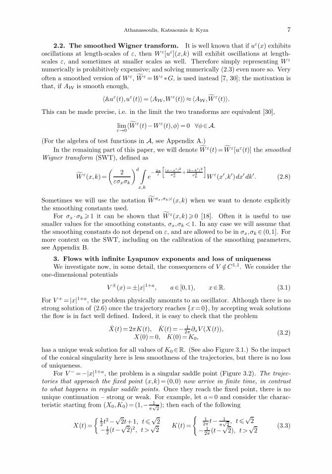
For V −=−|x|1+a, the problem is a singular saddle point (Figure 3.2). The trajec-tories that approach the fixed point (x,k)= (0,0) now arrive in finite time, in contrastto what happens in regular saddle points. Once they reach the fixed point, there is nounique continuation – strong or weak. For example, let a=0 and consider the charac-teristic starting from (X0,K0)= (1,− 1
π√2); then each of the following
X(t)=
12 t
2−√2t+1, t6
√2
− 12 (t−
√2)2, t>
√2
K(t)=
12π t− 1
π√2, t6
√2
− 12π (t−
√2), t>
√2
(3.3)
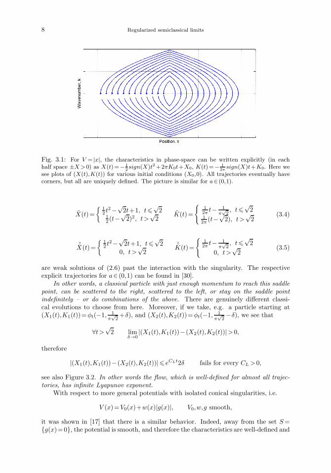
8 Regularized semiclassical limits
Fig. 3.1: For V = |x|, the characteristics in phase-space can be written explicitly (in eachhalf space ±X>0) as X(t)=− 1
2sign(X)t2+2πK0t+X0, K(t)=− 1
2πsign(X)t+K0. Here we
see plots of (X(t),K(t)) for various initial conditions (X0,0). All trajectories eventually havecorners, but all are uniquely defined. The picture is similar for a∈ (0,1).
X(t)=
12 t
2−√2t+1, t6
√2
12 (t−
√2)2, t>
√2
K(t)=
12π t− 1
π√2, t6
√2
12π (t−
√2), t>
√2
(3.4)
˜X(t)=
12 t
2−√2t+1, t6
√2
0, t>√2
˜K(t)=
12π t− 1
π√2, t6
√2
0, t>√2
(3.5)
are weak solutions of (2.6) past the interaction with the singularity. The respectiveexplicit trajectories for a∈ (0,1) can be found in [30].
In other words, a classical particle with just enough momentum to reach this saddlepoint, can be scattered to the right, scattered to the left, or stay on the saddle pointindefinitely – or do combinations of the above. There are genuinely different classi-cal evolutions to choose from here. Moreover, if we take, e.g. a particle starting at(X1(t),K1(t))=φt(−1, 1
π√2+δ), and (X2(t),K2(t))=φt(−1, 1
π√2−δ), we see that
∀t>√2 lim
δ→0|(X1(t),K1(t))−(X2(t),K2(t))|> 0,
therefore
|(X1(t),K1(t))−(X2(t),K2(t))|6 eCLt2δ fails for every CL> 0,
see also Figure 3.2. In other words the flow, which is well-defined for almost all trajec-tories, has infinite Lyapunov exponent.
With respect to more general potentials with isolated conical singularities, i.e.
V (x)=V0(x)+w(x)|g(x)|, V0,w,g smooth,
it was shown in [17] that there is a similar behavior. Indeed, away from the set S=g(x)=0, the potential is smooth, and therefore the characteristics are well-defined and
Athanassoulis, Katsaounis & Kyza 9
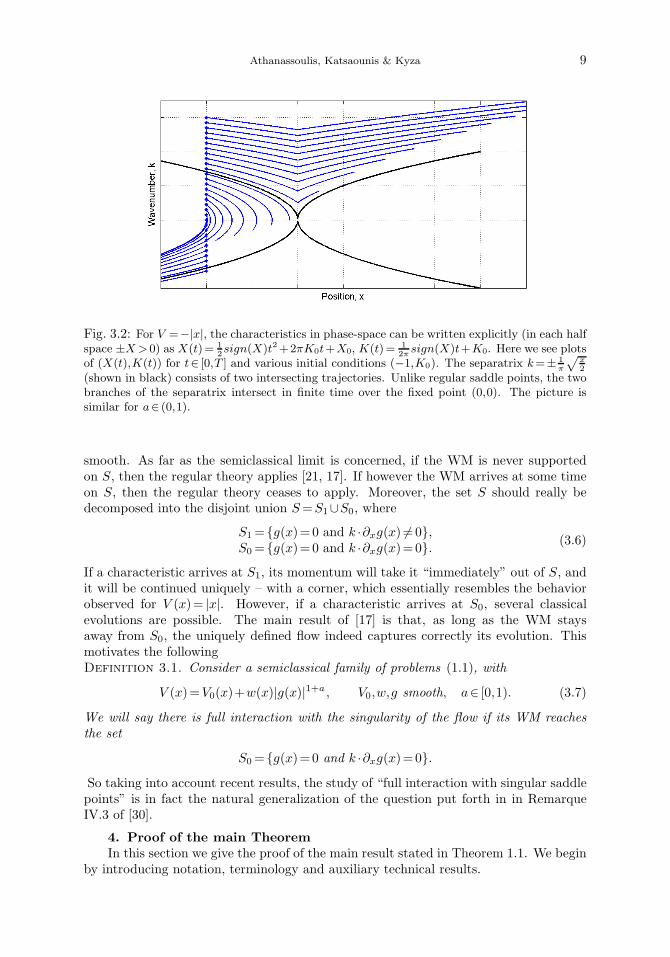
Fig. 3.2: For V =−|x|, the characteristics in phase-space can be written explicitly (in each halfspace ±X>0) as X(t)= 1
2sign(X)t2+2πK0t+X0, K(t)= 1
2πsign(X)t+K0. Here we see plots
of (X(t),K(t)) for t∈ [0,T ] and various initial conditions (−1,K0). The separatrix k=± 1
π
√x2
(shown in black) consists of two intersecting trajectories. Unlike regular saddle points, the twobranches of the separatrix intersect in finite time over the fixed point (0,0). The picture issimilar for a∈ (0,1).
smooth. As far as the semiclassical limit is concerned, if the WM is never supportedon S, then the regular theory applies [21, 17]. If however the WM arrives at some timeon S, then the regular theory ceases to apply. Moreover, the set S should really bedecomposed into the disjoint union S=S1∪S0, where
S1= g(x)=0 and k ·∂xg(x) 6=0,S0= g(x)=0 and k ·∂xg(x)=0. (3.6)
If a characteristic arrives at S1, its momentum will take it “immediately” out of S, andit will be continued uniquely – with a corner, which essentially resembles the behaviorobserved for V (x)= |x|. However, if a characteristic arrives at S0, several classicalevolutions are possible. The main result of [17] is that, as long as the WM staysaway from S0, the uniquely defined flow indeed captures correctly its evolution. Thismotivates the followingDefinition 3.1. Consider a semiclassical family of problems (1.1), with
V (x)=V0(x)+w(x)|g(x)|1+a , V0,w,g smooth, a∈ [0,1). (3.7)
We will say there is full interaction with the singularity of the flow if its WM reachesthe set
S0= g(x)=0 and k ·∂xg(x)=0.So taking into account recent results, the study of “full interaction with singular saddlepoints” is in fact the natural generalization of the question put forth in in RemarqueIV.3 of [30].
4. Proof of the main Theorem
In this section we give the proof of the main result stated in Theorem 1.1. We beginby introducing notation, terminology and auxiliary technical results.
10 Regularized semiclassical limits
4.1. Notations.
Definition 4.1 (Fourier transform). Given f(x) its Fourier transform is definedas
f(k) :=Fx→k[f ]=
∫e−2πix·kf(x)dx.
For functions on phase-space f(x,k), we will also use the Fourier transform in thesecond set of variables,
f2(x,K) :=Fk→K [f ]=F2f =
∫e−2πik·Kf(x,k)dk.
For the Fourier transform of functions of phase-space we will typically use the variables
f(X,K) :=Fx,k→X,K [f ]=Ff=
∫e−2πi[x·X+k·K]f(x,k)dxdk.
Definition 4.2 (Schwarz test functions). We will denote by S(Rd) the class offunctions φ :Rd→C for which
∀ multi-indices a,b ∃ Ca,b so that |xa∂bxφ(x)|6Ca,b.
As is well known, φ∈S(Rd)⇔φ∈S(Rd).Definition 4.3. For f ∈C1,a we define its norm by
‖f‖C1,a = supx1 6=x2
|∂xf(x1)−∂xf(x2)||x1−x2|a
+supx
|f(x)|+supx
|∂xf(x)|
Definition 4.4. For a,b∈C, we will use the notation a4 b with the understanding
a4 b ⇔|a|=O(|b|).
Definition 4.5. Denote by T (t) the free-space propagator on phase-space,
T (t) :f(x,k) 7→f(x−2πtk,k). (4.1)
Given any function f(x,k) on phase-space we denote for further reference
T Vε f :=
2
εRe
[i
∫e2πiSxV (S)f(x,k− εS
2)dS
], (4.2)
T V0 f := − 1
2π∂xV ·∂kf, (4.3)
T Vε f :=FT V
ε f =2
∫V (S)f(X−S,K)
sin(πεS ·K)
εdS, (4.4)
T (t)f(X,K) := F [T (t)f ]= f(X,K+2πXt), (4.5)
‖f‖FjLp := ‖Fjf‖Lp , for j∈1,2,∅. (4.6)
Athanassoulis, Katsaounis & Kyza 11
4.2. Auxiliary technical lemmata.
Observation 4.6. For any f,g functions on phase-space, t∈R we have
〈T (t)f,g〉= 〈f,T (−t)g〉, 〈T (t)f,g〉= 〈f, T (−t)g〉,
whenever the integrals exist. Moreover,
‖T (t)f‖FLp = ‖f‖FLp, ‖T (t)f‖FLp = ‖f‖FLp
for all p∈ [1,∞].Observation 4.7. If W =W ε[u](x,k) for some u with ‖u‖L2 =1, then
W2(x,K)=u(x− εK
2)u(x+
εK
2), ‖W2‖L∞
KL1
x=1
In particular, it follows that
〈W,φ〉4 ‖φ2‖L1KL∞
x6 ‖φ‖FL1 ⇒ W ∈B−M .
Lemma 4.1 (A specialized Liouville regularity estimate). Denote by E(t) the prop-agator for the Liouville equation (1.3), and assume that the potential V satisfies
V (S)|S| ∈L1.
Then there exists a constant CL> 0, depending on V and M , so that
|||ρ(t)|||M = |||E(t)ρ0|||M 6 eCL|t||||ρ0|||M .
Remark 4.8. The point of this result is that smoothness in k is in fact preserved bythe flow. In that sense, this lemma can be seen as a counterpart of Proposition 1 of[17].
Before we proceed to the proof , observe that the assumption V (S)|S| ∈L1 is alittle stronger than V ∈W 1,∞, but less strong than V ∈C1,1. For example if a∈ (0,1),V (x)=C|x|1+ab(x) (where b(x) is a smooth cutoff function of compact support, see,
e.g., the statement of Problem 4.11 in section 4.4) then V (S)|S| ∈L1 while V /∈C1,1.Such potentials in particular are the ones that appear in the example of Remarque IV.3of [30].
Proof : Without loss of generality, we prove the result for t> 0. We work in the Fourierdomain,
∂tρ−2πX ·∂K ρ+2π
∫
S
V (S)ρ(X−S,K)S ·KdS=0,
for some ρ0∈S∩BM . Now using T (t) and integrating in time, we can recast the Fourier-transformed Liouville equation in mild form, namely
ρ(t)= T (t)ρ0+2π
∫
τ=0
T (t−τ)
∫
S
S ·KV (S)ρ(X−S,K,τ)dS dτ.
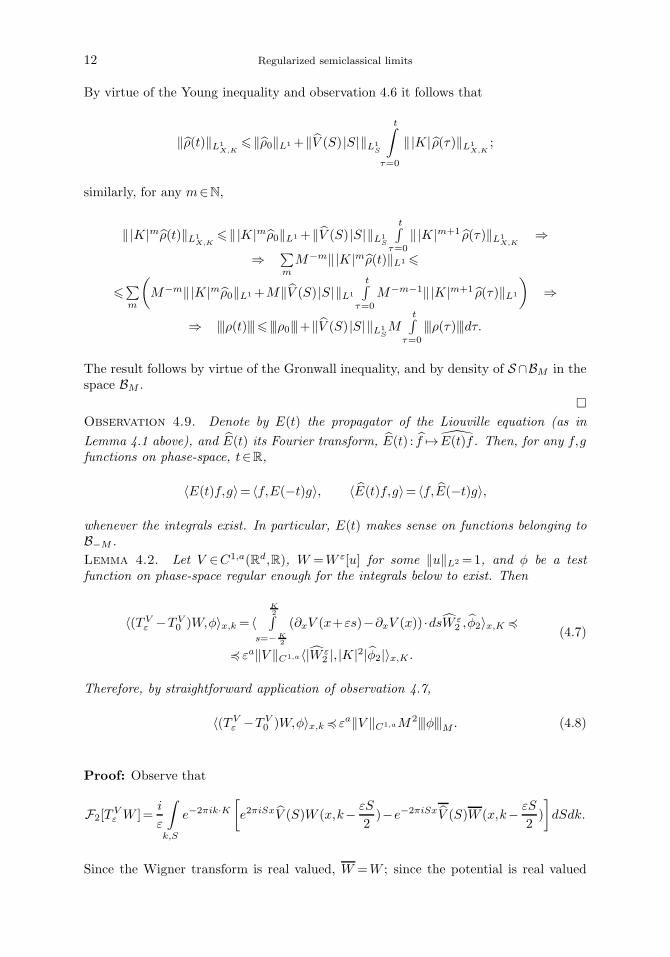
12 Regularized semiclassical limits
By virtue of the Young inequality and observation 4.6 it follows that
‖ρ(t)‖L1X,K
6 ‖ρ0‖L1 +‖V (S)|S|‖L1S
t∫
τ=0
‖|K| ρ(τ)‖L1X,K
;
similarly, for any m∈N,
‖|K|mρ(t)‖L1X,K
6 ‖|K|mρ0‖L1 +‖V (S)|S|‖L1S
t∫τ=0
‖|K|m+1 ρ(τ)‖L1X,K
⇒⇒ ∑
m
M−m‖|K|mρ(t)‖L1 6
6∑m
(M−m‖|K|mρ0‖L1 +M‖V (S)|S|‖L1
t∫τ=0
M−m−1‖|K|m+1 ρ(τ)‖L1
)⇒
⇒ |||ρ(t)|||6 |||ρ0|||+‖V (S)|S|‖L1SM
t∫τ=0
|||ρ(τ)|||dτ.
The result follows by virtue of the Gronwall inequality, and by density of S∩BM in thespace BM .
Observation 4.9. Denote by E(t) the propagator of the Liouville equation (as in
Lemma 4.1 above), and E(t) its Fourier transform, E(t) : f 7→ E(t)f . Then, for any f,gfunctions on phase-space, t∈R,
〈E(t)f,g〉= 〈f,E(−t)g〉, 〈E(t)f,g〉= 〈f,E(−t)g〉,
whenever the integrals exist. In particular, E(t) makes sense on functions belonging toB−M .
Lemma 4.2. Let V ∈C1,a(Rd,R), W =W ε[u] for some ‖u‖L2 =1, and φ be a testfunction on phase-space regular enough for the integrals below to exist. Then
〈(T Vε −T V
0 )W,φ〉x,k = 〈K2∫
s=−K2
(∂xV (x+εs)−∂xV (x)) ·dsW ε2 ,φ2〉x,K 4
4 εa‖V ‖C1,a〈|W ε2 |, |K|2|φ2|〉x,K .
(4.7)
Therefore, by straightforward application of observation 4.7,
〈(T Vε −T V
0 )W,φ〉x,k4 εa‖V ‖C1,aM2|||φ|||M . (4.8)
Proof: Observe that
F2[TVε W ]=
i
ε
∫
k,S
e−2πik·K[e2πiSxV (S)W (x,k− εS
2)−e−2πiSxV (S)W (x,k− εS
2)
]dSdk.
Since the Wigner transform is real valued, W =W ; since the potential is real valued
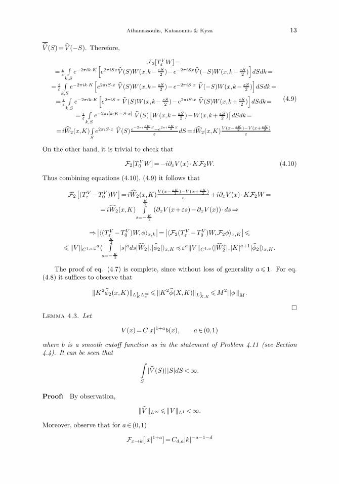
Athanassoulis, Katsaounis & Kyza 13
V (S)= V (−S). Therefore,
F2[TVε W ]=
= iε
∫k,S
e−2πik·K[e2πiSxV (S)W (x,k− εS
2 )−e−2πiSxV (−S)W (x,k− εS2 )]dSdk=
= iε
∫k,S
e−2πik·K[e2πiS·x V (S)W (x,k− εS
2 )−e−2πiS·x V (−S)W (x,k− εS2 )]dSdk=
= iε
∫k,S
e−2πik·K[e2πiS·x V (S)W (x,k− εS
2 )−e2πiS·x V (S)W (x,k+ εS2 )]dSdk=
= iε
∫k,S
e−2πi[k·K−S·x] V (S)[W (x,k− εS
2 )−W (x,k+ εS2 )]dSdk=
= iW2(x,K)∫S
e2πiS·x V (S) e−2πi εK
2S−e
2πi εK2
S
εdS= iW2(x,K)
V (x− εK2 )−V (x+ εK
2 )
ε
(4.9)
On the other hand, it is trivial to check that
F2[TV0 W ]=−i∂xV (x) ·KF2W. (4.10)
Thus combining equations (4.10), (4.9) it follows that
F2
[(T V
ε −T V0 )W
]= iW2(x,K)
V (x− εK2 )−V (x+ εK
2 )
ε+ i∂xV (x) ·KF2W =
= iW2(x,K)
K2∫
s=−K2
(∂xV (x+εs)−∂xV (x)) ·ds⇒
⇒∣∣〈(T V
ε −T V0 )W,φ〉x,k
∣∣=∣∣〈F2(T
Vε −T V
0 )W,F2φ〉x,K∣∣6
6 ‖V ‖C1,aεa〈K2∫
s=−K2
|s|ads|W2|, |φ2|〉x,K 4 εa‖V ‖C1,a〈|W ε2 |, |K|a+1|φ2|〉x,K .
The proof of eq. (4.7) is complete, since without loss of generality a6 1. For eq.(4.8) it suffices to observe that
‖K2φ2(x,K)‖L1KL∞
x6 ‖K2φ(X,K)‖L1
X,K6M2|||φ|||M .
Lemma 4.3. Let
V (x)=C|x|1+ab(x), a∈ (0,1)
where b is a smooth cutoff function as in the statement of Problem 4.11 (see Section4.4). It can be seen that
∫
S
|V (S)| |S|dS<∞.
Proof: By observation,
‖V ‖L∞ 6 ‖V ‖L1 <∞.
Moreover, observe that for a∈ (0,1)
Fx→k[|x|1+a]=Cd,a|k|−a−1−d
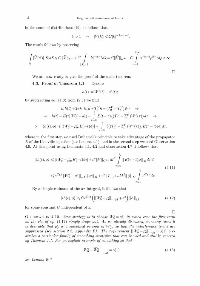
14 Regularized semiclassical limits
in the sense of distributions [19]. It follows that
|k|> 1 ⇒ |V (k)|6C|k|−1−a−d.
The result follows by observing
∫
S
|V (S)| |S|dS6C‖V ‖L∞ +C
∫
|S|>1
|k|−a−ddk=C‖V ‖L∞ +C
+∞∫
ρ=1
ρ−a−dρd−1dρ<∞.
We are now ready to give the proof of the main theorem.
4.3. Proof of Theorem 1.1. Denote
h(t) :=W ε(t)−ρε(t);
by subtracting eq. (1.3) from (2.3) we find
∂th(t)+2πk ·∂xh+T V0 h=(T V
0 −T Vε )W ε ⇒
⇒ h(t)=E(t)(W ε0 −ρε0)+
t∫τ=0
E(t−τ)((T V
0 −T Vε )W ε(τ)
)dτ ⇒
⇒ |〈h(t),φ〉|6 |〈W ε0 −ρε0,E(−t)φ〉|+
t∫τ=0
∣∣〈((T V
0 −T Vε )W ε(τ)
),E(τ − t)φ〉
∣∣dτ,
where in the first step we used Duhamel’s principle to take advantage of the propagatorE of the Liouville equation (see Lemma 4.1), and in the second step we used Observation4.9. At this point using Lemmata 4.1, 4.2 and observation 4.7 it follows that
|〈h(t),φ〉|6 |〈W ε0 −ρε0,E(−t)φ〉|+εa‖V ‖C1,aM2
t∫
τ=0
|||E(τ− t)φ|||Mdτ 6
6 eCLt|||W ε0 −ρε0|||−M |||φ|||M +εa‖V ‖C1,aM2|||φ|||M
t∫
τ=0
eCLτdτ.
(4.11)
By a simple estimate of the dτ integral, it follows that
|〈h(t),φ〉|6CeCLt(|||W ε
0 −ρε0|||−M +εa)|||φ|||M (4.12)
for some constant C independent of ε.
Observation 4.10. One strategy is to choose W ε0 =ρε0, in which case the first term
on the rhs of eq. (4.12) simply drops out. As we already discussed, in many cases itis desirable that ρε0 is a smoothed version of W ε
0 , so that the interference terms aresuppressed (see section 2.2, Appendix B). The requirement |||W ε
0 −ρε0|||−M = o(1) pre-scribes a particular family of smoothing strategies that can be used and still be coveredby Theorem 1.1. For an explicit example of smoothing so that
∣∣∣∣∣∣∣∣∣W ε
0 −W ε0
∣∣∣∣∣∣∣∣∣−M
= o(1) (4.13)
see Lemma B.3.
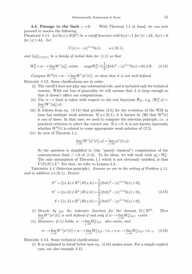
Athanassoulis, Katsaounis & Kyza 15
4.4. Passage to the limit ε→0. With Theorem 1.1 at hand, we can nowproceed to resolve the followingProblem 4.11. Let b(x)∈S(Rd) be a cutoff function with b(x)=1 for |x|< 2L, b(x)=0for |x|> 4L. Let
V (x)=−|x|1+ab(x), a∈ [0,1),
and uε0ε∈(0,1) be a family of initial data for (1.1) so that
W 00 =w−∗ lim
ε→0W ε[uε
0] exists, suppW 00 ∩1
2(2πk)2−|x|1+ab(x)=0 6= ∅. (4.14)
Compute W 0(t)=w−∗ limε→0
W ε[uε(t)], or show that it is not well-defined.
Remark 4.12. Some clarifications are in order:(i) The cutoff b does not play any substantial role, and is included only for technical
reasons. With out loss of generality we will assume that L is large enough sothat it doesn’t affect our computations.
(ii) The w−∗ limit is taken with respect to the test functions BM , e.g, 〈W 00 ,φ〉=
limε→0
〈W ε[uε0],φ〉.
(iii) It follows from eq. (4.14) that problem (2.5) for the evolution of the WM intime has multiple weak solutions. If a∈ (0,1), it is known by [30] that W 0(t)is one of these. In that case, we need to compute the selection principle, i.e. apractical criterion to select the correct one. If a=0, it is not known rigorouslywhether W 0(t) is related to some appropriate weak solution of (2.5).
(iv) In view of Theorem 1.1,
limε→0
〈W ε[uε(t)],φ〉= limε→0
〈ρε(t),φ〉.
So the question is simplified to (the “purely classical”) computation of theconcentration limit ε→0 of (1.3). To fix ideas, we will work with ρε0=W ε
0 .The only assumption of Theorem 1.1 which is not obviously satisfied, is thatV (S)|S| ∈L1. For that, we refer to Lemma 4.3.
Theorem 4.4 (Selection principle). Assume we are in the setting of Problem 4.11,and in addition a∈ (0,1). Denote
S+= (x,k)∈R2 |H(x,k)=1
2(2πk)2−|x|1+ab(x)> 0,
S−= (x,k)∈R2 |H(x,k)=1
2(2πk)2−|x|1+ab(x)< 0,
S= (x,k)∈R2 |H(x,k)=1
2(2πk)2−|x|1+ab(x)=0.
(4.15)
(i) Denote by χΩ the indicator function for the domain Ω⊆R2d. Thenlimε→0
W ε[uε(t)] is well defined if and only if w−∗ limε→0
W ε0χS+ exists.
(ii) Moreover, if (i) holds, w−∗ limε→0
W ε0χS− also exists, and
w−∗ limε→0
W ε[uε(t)]=w−∗ limε→0
W ε0χS− φ−t+w−∗ lim
ε→0W ε
0χS+ φ−t. (4.16)
Remark 4.13. Some technical clarifications:(i) It is explained in detail below how eq. (4.16) makes sense. For a simple explicit
case, see also example 4.15.
16 Regularized semiclassical limits
(ii) In [30] it is discussed in some detail how w−∗ limε→0
W ε0χS+ may fail to exist.
(iii) We will make some standard additional regularity assumptions on the initialdata, namely
∀ε, max|a|,|b|6d+1
‖xa∂bxu
ε0(x)‖L2 <∞.
This is sufficient to assure that ρε0=W ε0 ∈L1(R2d)∩L∞(R2d); see Theorem A.3.
Although this is not strictly necessary, it simplifies considerably some technicalpoints in the proof below.
Proof of Theorem 4.4: Phase space was partitioned into the disjoint union R2=S+∪S∪S− in eq. (4.15), accordingly
ρε0=ρε++ρε−+ρεz, where ρε±=ρε0χS± , ρεz =ρε0χS .
Since ρε0∈L1∩L∞ and S is of measure zero, it follows automatically that ρεz =0. There-fore ρε0=ρε++ρε−, and it suffices to solve each of the problems
∂tρε+(t)+2πk ·∂xρε+(t)−
1
2π∂xV ·∂kρε+(t)=0, ρε(t=0)=ρε+, (4.17)
∂tρε−(t)+2πk ·∂xρε−(t)−
1
2π∂xV ·∂kρε−(t)=0, ρε(t=0)=ρε−, (4.18)
separately. The point, of course, is that by construction, ρε± φ−t stays supported insideS±, ∀t∈R, ε∈ (0,1). The restriction of the flow φt on each of the sets S+, S−, will bedenoted by φ+
t , φ−t respectively.
Claim 4.14. The flow φ±t is well-defined and continuous, i.e.
φ±t ∈C(S±,S±) ∀t> 0.
Proof of the claim: It follows in exactly the same way as Proposition 1 of [17].
Therefore each of φ±t can be extended to the closure of its domain. By abuse of
notation (but without real danger of confusion) we will denote this extension as φ±t
φ±t ∈C(S±,S±) ∀t> 0.
So in solving each of (4.17), (4.18) we will work exclusively on the respective domainsS±. Thus, for f ∈S(S±)
〈ρε± φ±t ,f〉= 〈ρε±,f φ±
t 〉 (4.19)
To conclude we observe that since ρε=ρε++ρε−, and we know that w−∗ limερε exists,
then necessarily w−∗ limερε− exists if and only if w−∗ lim
ερε+ exists. In that case, and
observing that f φ±t stays continuous for all times,
limε→0
〈ρε±(t),f〉= 〈 limε→0
ρε±,f φ±t 〉
For the same reason, if w−∗ limερε+ doesn’t exist, we cannot pass to the ε→0 limit
of eq. (4.19).
Athanassoulis, Katsaounis & Kyza 17
The proof of Theorem 4.4 is now complete.
It is clear that if Theorem 1.1 was valid for a=0, then Theorem 4.4 would follow,with the same proof. This is the motivation behind the numerical investigation of itsvalidity for a=0 which follows in the next sections.
Now, let us look at a concrete example:Example 4.15. Assume we are in the setting of Theorem 4.4, we take d=1 and let
uε0= ε−
14 e
−π2
(
x−x0√ε
)2+im(ε)
√|x0|1+a(x−x0)
ε
for some x0< 0. If limε→0
m(ε)=1, then the WM is
W 00 =w−∗ lim
ε→0W ε[uε
0]= δ(x−x0,k−√2|x0|1+a
2π)
is supported on the separatrix S. Since W ε0 is a Gaussian in phase space with an
effective support of O(ε12 ), it follows that if e.g., m(h)=1+ε
16 sin(1
ε), then w−∗ lim
ερε±
doesn’t exist, since the mass of W ε0 oscillates between S+ and S−. If, on the other
hand, m(h)=1+ε6sin(1ε), then the oscillations would be negligible in the limit, and
w−∗ limερε± exists.
Related examples can also be found in [5, 6].
5. The numerical method
5.1. Solving the semiclassical Schrodinger equation with conical singu-
larities. The numerical solution of (1.1) is complicated from the theoretical as well asfrom the practical point of view. The main difficulty is that the solution of (1.1) oscil-lates with wavelength O(ε) thus standard numerical methods require very fine meshes(space and time) to resolve adequately this high oscillatory behavior. Further the so-lution might exhibit caustics, making its numerical approximation even more difficult.Finally the relatively low smoothness of the potential V means that several tools widelyused in the numerical analysis and simulation of such problems are now not available.
Popular methods for the numerical solution of (1.1) are time-splitting spectral meth-ods and Crank-Nicolson finite element / finite difference methods. The standard Crank-Nicolson finite element / finite difference methods suffer from a very restrictive dispersiverelation, cf. [25], connecting the space and time mesh sizes with the parameter ε thus re-quiring considerable computational resources in order to produce accurate solutions forε≪1. In an attempt to relax this restrictive dispersive relation Bao, Jin and Markowichin [10] proposed time-splitting spectral methods for the numerical solution of (1.1). Thisis widely considered to be the preferred approach for semiclassical problems; however itrequires V ∈C2 at least for any kind of rigorous convergence result.
A different approach to overcome this difficulty is based on adaptivity. Adaptivemethods are widely used in recent years to construct accurate numerical approximationsto a broad class of problems with substantially reduced computational cost by creatingappropriately nonuniform meshes in space and time. There are several ways to proposean adaptive strategy. One such approach is based on rigorous a posteriori error control.The idea is to estimate the error in some natural norm by
‖u−U‖≤E(U) (5.1)
18 Regularized semiclassical limits
where E(U) a computable quantity depending on the approximate solution U and thedata of the problem. A crucial property that the estimator E(U) must satisfy, is to con-verge with the same order as the numerical method. It is then said that E(U) decreaseswith optimal order with respect to the mesh discretization parameters. The existingliterature on adaptive methods based on a posteriori error bounds for the numericalapproximation of (1.1) is very limited. Very recently the authors presented in [26], anadaptive algorithm for the numerical approximation of (1.1), based on a posteriori errorestimates of optimal order. The proposed adaptive method proved to be competitivewith the best available methods in the literature not only for the approximation of thesolution of (1.1) but as well as for its observables, c.f. [26].
Here we want to investigate the behavior of a quantum problem, for which we don’thave even any qualitative a priori information. (E.g. the percentage of mass scatteredin different directions after the interaction with the singularity.) Hence a posteriorierror control is particularly useful, as it provides a rigorous, quantitative grasp on thequantum interaction – making meaningful the subsequent comparison to the classicalasymptotics.
5.2. The CNFE method. In [26] the authors consider the initial-and-boundaryvalue problem
iεuεt +
ε2
2∆uε−V uε= f in Ω×(0,T ],
uε=0 on ∂Ω× [0,T ],
uε(t=0)=uε0 in Ω,
(5.2)
where Ω⊂Rd is a bounded domain and f ∈L∞([0,T ];L2(Ω))is a forcing term. They
discretize (5.2) by a Crank-Nicolson finite element (CNFE) scheme and prove a poste-riori error estimates of optimal order. One of the main features of the considered finiteelement spaces is that they are allowed to change in time. The optimal order a posteriorierror bounds are derived in the L∞
t L2x norm and the analysis includes time-dependent
potentials. Furthermore the derived a posteriori estimates are valid for L∞t L∞
x -type po-tentials as well, in contrast to the existing results in the literature which require smoothC1
t C2x-type potentials.The analysis in [26] is based on the reconstruction technique, proposed by Akrivis,
Makridakis & Nochetto, for the heat equation, cf. [1, 31]. In [26] the authors, follow-ing this technique, introduce a novel time-space reconstruction for the CNFE scheme,appropriate for the Schrodinger equation (5.2). A posteriori estimates for (5.2) and theCNFE method were also proven by Dofler in [14], but the estimator was not of optimalorder in time.
The main results of [26] can be summarized as follows: The approximations Un(x) ofuε(x,tn), 0≤n≤N, are computed for a non-uniform time grid 0=: t0<t1< · · ·<tN =:T of [0,T ]. For each n, Un belongs to a finite element space (which depends on n)consisting of piecewise polynomials of degree r. By U(x,t) we denote the piecewiselinear interpolant between the nodal values Un. More specifically, for t∈ [tn−1,tn],
U(x,t) :=t− tn−1
tn− tn−1Un(x)+
tn− t
tn− tn−1Un−1(x). Then
‖(uε−U)(t)‖L2(Ω)≤E0N +ES
N +ETN , ∀t∈ [0,T ], (5.3)
where E0N , ES
N , ETN are all computable quantities. More precisely, E0
N accounts forthe initial error, while ES
N , ETN are the space and time estimators respectively. These
Athanassoulis, Katsaounis & Kyza 19
estimators are used to refine appropriately the time and space mesh sizes, thus creatingan adaptive algorithm. The algorithm is said to converge up to a preset tolerance Tolif, after appropriate refinements, we obtain an approximate solution U of u with
E0N +ES
N +ETN <Tol.
In particular, in view of (5.3), we will then have that
‖(uε−U)(t)‖L2(Ω)≤Tol, ∀t∈ [0,T ]. (5.4)
The adaptive algorithm of [26] provides efficient error control for the solution andits observables for small values of Planck’s constant ε, and in particular reduces sub-stantially the computational cost as compared to uniform meshes. It is very difficultto obtain such results via standard techniques and without adaptivity, especially whennon-smooth potentials are considered. In addition, it is to be emphasized that as longas the adaptive algorithm converges, we can guarantee rigorously, based on the a pos-teriori error analysis, that the total L∞
t L2x error remains below a given tolerance, Tol.
For more details, see [26].
5.3. Validation of the CNFE scheme. We consider the one-dimensionalspatial case of (5.2), Ω=(a,b), and we proceed to a series of numerical experimentswhich (a) validate the method and the estimators in (5.3) in terms of accuracy and(b) highlight the advantages of adaptivity. We consider the numerical solution of (5.2),obtained by the CNFE scheme, with initial condition
uε0(x)=a0(x)e
iS0(x)
ε ,
where a0 may or may not depend on ε. For the spatial discretization we use finite elementspaces consisting of B-splines of degree r, r∈N. The theoretical order of convergence forthe CNFE scheme is 2 in time and r+1 in space; thus the expected order of convergenceof the estimator ES
N is r+1 and of ETN is 2.
Next, our purpose is to verify numerically the aforementioned order of convergencefor the estimators, for smooth and non-smooth potentials V . To this end, let ℓ∈N countthe different realizations (runs) of the experiments. We consider uniform partitions inboth time and space, and let M(ℓ)+1 and N(ℓ)+1 denote the number of nodes in space
(of [a,b]) and in time (of [0,T ]), respectively. Then ∆x(ℓ) :=b−a
M(ℓ)and ∆t(ℓ) :=
T
N(ℓ)denote the space and time discretization parameters (of the ℓth realization), respectively.The experimental order of convergence (EOC) s computed for the space estimator ES
N
as follows:
EOCS :=log(ESN (ℓ)/ES
N(ℓ+1))
log(M(ℓ+1)/M(ℓ)
) , (5.5)
where ESN (ℓ) and ES
N (ℓ+1) denote the values of the space estimators in two consecutiveimplementations with mesh sizes ∆x(ℓ) and ∆x(ℓ+1), respectively. Similarly, for thetime estimator ET
N the EOC is computed as
EOCT :=log(ETN (ℓ)/ET
N(ℓ+1))
log(N(ℓ+1)/N(ℓ)
) . (5.6)
20 Regularized semiclassical limits
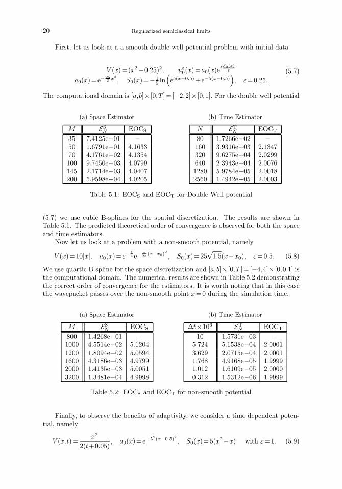
First, let us look at a a smooth double well potential problem with initial data
V (x)= (x2−0.25)2, uε0(x)=a0(x)e
iS0(x)
ε
a0(x)=e−252 x2
, S0(x)=− 15 ln(e5(x−0.5)+e−5(x−0.5)
), ε=0.25.
(5.7)
The computational domain is [a,b]× [0,T ]= [−2,2]× [0,1]. For the double well potential
(a) Space Estimator
M ESN EOCS
35 7.4125e−01 –50 1.6791e−01 4.163370 4.1761e−02 4.1354100 9.7450e−03 4.0799145 2.1714e−03 4.0407200 5.9598e−04 4.0205
(b) Time Estimator
N ETN EOCT
80 1.7266e−02 –160 3.9316e−03 2.1347320 9.6275e−04 2.0299640 2.3943e−04 2.00761280 5.9784e−05 2.00182560 1.4942e−05 2.0003
Table 5.1: EOCS and EOCT for Double Well potential
(5.7) we use cubic B-splines for the spatial discretization. The results are shown inTable 5.1. The predicted theoretical order of convergence is observed for both the spaceand time estimators.
Now let us look at a problem with a non-smooth potential, namely
V (x)=10|x|, a0(x)= ε−14 e−
π2ε (x−x0)
2
, S0(x)=25√1.5(x−x0), ε=0.5. (5.8)
We use quartic B-spline for the space discretization and [a,b]× [0,T ]= [−4,4]× [0,0.1] isthe computational domain. The numerical results are shown in Table 5.2 demonstratingthe correct order of convergence for the estimators. It is worth noting that in this casethe wavepacket passes over the non-smooth point x=0 during the simulation time.
(a) Space Estimator
M ESN EOCS
800 1.4268e−01 –1000 4.5514e−02 5.12041200 1.8094e−02 5.05941600 4.3186e−03 4.97992000 1.4135e−03 5.00513200 1.3481e−04 4.9998
(b) Time Estimator
∆t×106 ETN EOCT
10 1.5731e−03 –5.724 5.1538e−04 2.00013.629 2.0715e−04 2.00011.768 4.9168e−05 1.99991.012 1.6109e−05 2.00000.312 1.5312e−06 1.9999
Table 5.2: EOCS and EOCT for non-smooth potential
Finally, to observe the benefits of adaptivity, we consider a time dependent poten-tial, namely
V (x,t)=x2
2(t+0.05), a0(x)=e−λ2(x−0.5)2 , S0(x)=5(x2−x) with ε=1. (5.9)
Athanassoulis, Katsaounis & Kyza 21
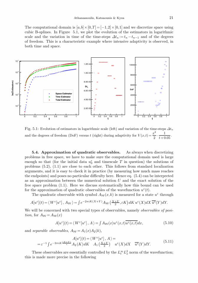
The computational domain is [a,b]× [0,T ]= [−1,2]× [0,1] and we discretize space usingcubic B-splines. In Figure 5.1, we plot the evolution of the estimators in logarithmicscale and the variation in time of the time-steps ∆tn := tn− tn−1 and of the degreesof freedom. This is a characteristic example where intensive adaptivity is observed, inboth time and space.
t
ln(Estimators)
0 0.2 0.4 0.6 0.8 1
10-5
10-4
10-3
10-2
10-1
Space Estimator
Time Estimator
Total Estimator
t0 0.2 0.4 0.6 0.8 1
2.0E-05
4.0E-05
6.0E-05
8.0E-05
1.0E-04
1.2E-04
Dtn
t0 0.2 0.4 0.6 0.8 1
0
2000
4000
6000
8000
10000
DoF
Fig. 5.1: Evolution of estimators in logarithmic scale (left) and variation of the time-steps ∆tn
and the degrees of freedom (DoF) versus t (right) during adaptivity for V (x,t)=x2
2·
1
t+0.05.
5.4. Approximation of quadratic observables. As always when discretizingproblems in free space, we have to make sure the computational domain used is largeenough so that (for the initial data uε
0 and timescale T in question) the solutions ofproblems (5.2), (1.1) are close to each other. This follows from standard localizationarguments, and it is easy to check it in practice (by measuring how much mass reachesthe endpoints) and poses no particular difficulty here. Hence eq. (5.4) can be interpretedas an approximation between the numerical solution U and the exact solution of thefree space problem (1.1). Here we discuss systematically how this bound can be usedfor the approximation of quadratic observables of the wavefunction uε(t).
The quadratic observable with symbol AW (x,k) is measured for a state uε through
A[uε](t)= 〈W ε[uε] , AW 〉=∫e−2πiK(X+Y )AW
(X+Y
2 ,εK)dK uε(X)dX uε(Y )dY.
We will be concerned with two special types of observables, namely observables of posi-tion, for AW =AW(x)
A[uε](t)= 〈W ε[uε] , A 〉=∫AW(x)uε(x,t)uε(x,t)dx, (5.10)
and separable observables, AW =A1(x)A2(k),
A[uε](t)= 〈W ε[uε] , A 〉== ε−1
∫e−2πiK (X+Y )
ε A2 (K)dK A1
(X+Y
2
)uε(X)dX uε(Y )dY.
(5.11)
These observables are essentially controlled by the L∞t L2
x norm of the wavefunction;this is made more precise in the following
22 Regularized semiclassical limits
Lemma 5.1 (Approximation of observables). If ‖uε−U‖L2 6Tol as in (5.4), thenfor every observable of position
|A[uε](t)−A[U ](t)|6Tol(‖U‖L2 +‖uε‖L2)‖AW‖L∞ =O(Tol), (5.12)
while for any separable observable
|A[uε](t)−A[U ](t)|6 ε−12Tol(‖U‖L2 +‖uε‖L2)‖AW‖L2 =O(ε−
12Tol). (5.13)
The proof follows by inspection of equations (5.10), (5.11).
Remark 5.1. The estimate (5.13) is far from sharp; in fact for regular, localized ob-
servables the ε−12 is very pessimistic. Still, carrying out rigorously a sharper microlocal
estimate for a non-smooth problem is outside the scope of this work. We note that, evenin an imperfect way, it is seen rigorously that the L2 approximation of the wavefunctiondoes indeed control the observables.
5.5. Particles for the Liouville equation. To approximate numerically thesolution of (1.3), we use a particle method; decompose the initial condition
ρε0≈N∑
j=1
Mjδ(x−Xj ,k−Kj);
then the center of each particle moves along its respective trajectory, in accordance to(2.6). (See also the caption of Figure 3.2 for an explicit form of the trajectories.) Thus
ρε(t)≈P ε(t)=
N∑
j=1
Mjδ(x−Xj(t),k−Kj(t)).
The advantage in this case is that we know explicitly the trajectories, and therefore
〈ρε(t)−P ε(t),φ〉= 〈ρε0−P ε(0),φ〉.
This makes it easy to generate approximations of observables of ρε(t), i.e.
∫ρε(x,k,t)AW (x,k)dxdk≈
∑
j
MjAW (Xj(t),Kj(t))
with predetermined accuracy.
6. Numerical results
In this section we present a series of one-dimensional numerical experiments, inves-tigating whether an appropriate version of Theorem 1.1 can be seen to hold for a=0,i.e. if
〈W ε[uε(t)]−ρε(t),φ〉= o(1) (6.1)
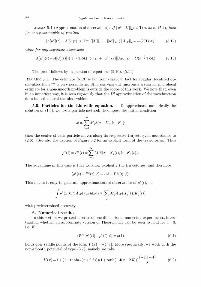
holds over saddle points of the form V (x)=−C|x|. More specifically, we work with thenon-smooth potential of type (3.7), namely we take
V (x)=1+(1+tanh(4(x+2.5)))(1+tanh(−4(x−2.5)))(−|x|+4)
8. (6.2)
Athanassoulis, Katsaounis & Kyza 23
-6 -4 -2 0 2 4 6
x
-1
0
1
2
3
4
V(x
)
Fig. 6.1: The non-smooth potential V of eq. (6.2).
This potential incorporates the non-smoothness at x=0 with a smooth transition to aconstant value away from it. Note that in a neighborhood of x=0, V is exponentially
close to − |x|2 +3, see Figure 6.1.
We compute the numerical solution of problem (5.2), which is known to approxi-mate well problem (1.1) as long as the effective support of the solution doesn’t reach theboundary of the computational domain. It will be referred to as the “exact wavefunc-tion”, and denoted by uε in the sequel. (“Exact” in the sense that the full, quantumdynamics are used.) The wavefunction uε is computed with a prescribed error toleranceof Tol≈ 0.01 (more specifically Tol∈ [0.005,0.02]).
We also compute the numerical solution to (1.3) with initial data ρε0= W ε0 , i.e. a
smoothing of W ε0 . We write for future reference
∂tρε(t)+2πk ·∂xρε(t)−
1
2π∂xV ·∂kρε(t)=0, ρε(t=0)= W ε
0 . (6.3)
This will be referred to as the “classical SWT”, and denoted by ρε(t) in the sequel. Aswas discussed in section 5.5, (almost all) the trajectories can be computed explicitly.The initial data uε
0 are chosen so that there is full interaction with the singularity ofthe flow, in the sense of definition 3.1.
So we have two reliable computations; one for the full quantum dynamics of theproblem, and one for a semiclassical model inspired by Theorem 1.1. We proceed tomeasure a number of observables against uε(t), ρε(t) before, during, and after interactionwith the saddle point. This is equivalent to checking whether eq. (6.1) holds for anumber of test functions (the Weyl symbols of the observables).
In the process of setting up the numerical experiments and interpreting the results, aclear dichotomy arises between problems with and without interference. A brief, precisedefinition can be given as follows:Definition 6.1. Given uε
0, V consider the problem
∂tfε(t)+2πk ·∂xf ε(t)− 1
2π∂xV ·∂kf ε(t)=0, f ε(t=0)=W ε[uε
0]. (6.4)
We say that interference is observed on a point (x∗,k∗) of phase-space if (non-negligiblefor ε= o(1)) amounts of mass of f arrive to (x∗,k∗) at the same time from differentdirections.
Clearly, interference is only possible where two trajectories intersect in finite time.For our potential V as in eq. (6.2), this is only the point (0,0). If one wavepacket
24 Regularized semiclassical limits
approaches (0,0) from one side, there is no interference going on. Interference would betaking place if two wavepackets arrive on (0,0), one from the right and one from theleft, at the same time.
6.1. Non-interference problems. For values of ε ranging from 5 ·10−1 to5 ·10−3, we simulate the evolution in time of wavepackets of the form
u0(x)=a0(x)eim
S0(x)
ε , a0(x)= ε−14 e
−π2 (
x−x0√ε
)2, S0(x)=
√|x0|(x−x0), (6.5)
for x0=−1.5, m∈ [0.8165,1.4289].
When m=1, the SWT W ε[uε] of this problem is centered on (−1.5,√
32 ); this point
reaches zero in t=√6, and roughly half the mass of the quantum particle – should (6.1)
hold – is expected to pass to x> 0, while the other half should reach close to x=0and then be reflected back to x< 0. By perturbing the value of m in the initial data,the amount of mass expected to cross over to x> 0 changes (from no mass crossingover, to all the mass crossing over in the extreme cases). In all of these case studies theinteraction with the singularity starts around t=1.3 and is over around t=2.45. Thuse.g. before the interaction with x=0 the classical and quantum solutions should agreevery well, which provides one more opportunity to validate and check our computations.We look at ρε(t) and W ε[uε(t)] in phase space, and we measure the observables withsymbols
Aα,β,j(x,k)=xα kβ χ[0,4]((−1)jx)χ[−1,1](k), α,β∈N0, α+β6 2, j∈1,2. (6.6)
The precise measurement of these observables corresponds to
〈W ε , xαkβ χ[0,4]((−1)jx)χ[−1,1](k) 〉=
=
∫e−2πiK(X+Y )
[χ[0,4]((−1)j
X+Y
2)χ[−1,1](εK)(
X+Y
2)α(εK)β
]dK uε(X)dX uε(Y )dY.
For β=0 these are observables of position only, so by the estimate (5.12) we have avery good approximation. For β> 0 we do not attempt to saturate the estimate (5.13),since it is quite clear from the numerical results that it is not necessary. Our findingsare fully consistent for both types of observables, as we will see below.
The agreement we find between the quantum dynamics and the proposed semiclas-sical asymptotics is striking already from relatively large values of ε. This is not entirelyunexpected, as away from x=0 the Liouville equation (2.5) is in fact identical with thefull quantum dynamics (2.3). The finding is that “nothing non-classical happens” onx=0 either, as can be clearly seen in Figures 6.2, 6.3 and 6.5.
Qualitatively this behavior also appeared in investigating problems with differentenvelopes and other values of ε. This creates a compelling sense that in non-interferenceproblems, eq. (6.1) is valid. In Appendix C an even more singular example can be seento be correctly captured by the regularized semiclassical asymptotics.
6.2. Collision of two wave packets. Since this is an one-dimensional problem,the only way to have interference is by one wavepacket arriving to x=0 from the left,and one from the right at the same time. So we consider the collision of two wavepackets, symmetrically located around x=0, traveling with same velocities and oppositedirections. The two wavepackets have a phase difference of an angle 2πθ, 0≤ θ≤ 1.They meet over the corner point of the potential, they interact and continue to travelin opposite directions until they are completely separated.
Athanassoulis, Katsaounis & Kyza 25
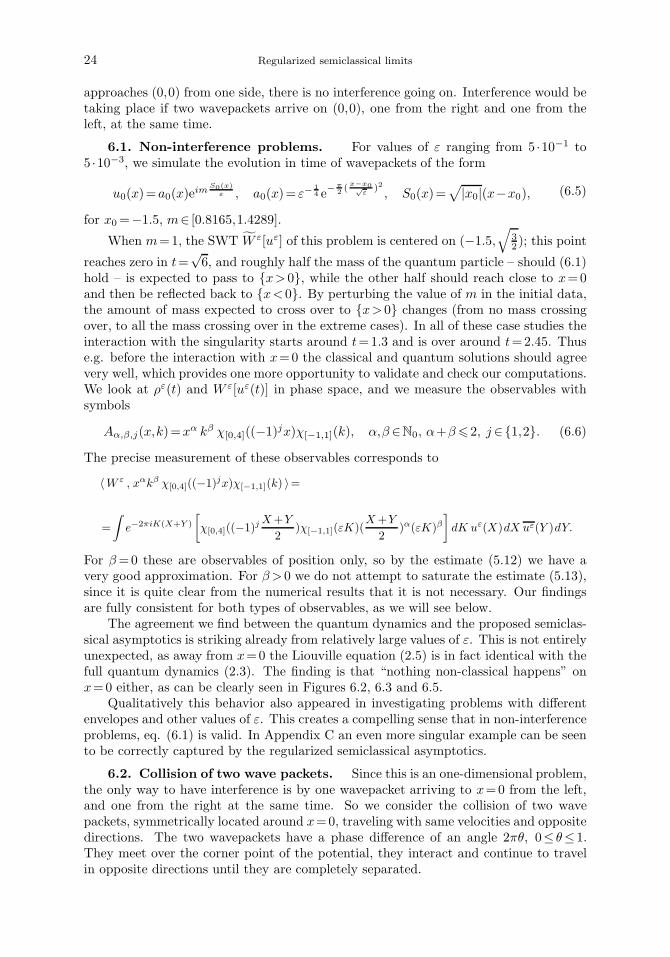
Fig. 6.2: Numerical result for ε=10−2, m=0.9186. Top right: Exact SWT. Top left: momen-tum density (dx integral of SWT). Bottom right: position density (dk integral of the SWT).Bottom left: ρε(t). (Note that in the SWT plots the wavenumber is scaled with 1
2π.)
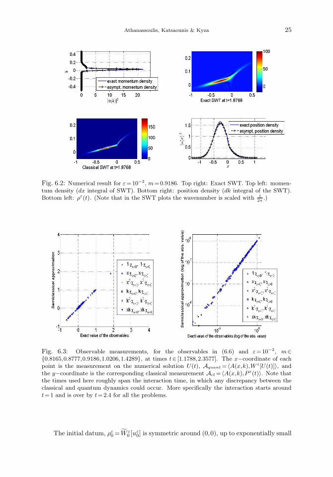
Fig. 6.3: Observable measurements, for the observables in (6.6) and ε=10−2, m∈0.8165,0.8777,0.9186,1.0206,1.4289, at times t∈ [1.1788,2.3577]. The x−coordinate of eachpoint is the measurement on the numerical solution U(t), Aquant= 〈A(x,k),W ε[U(t)]〉, andthe y−coordinate is the corresponding classical measurement Acl= 〈A(x,k),P ε(t)〉. Note thatthe times used here roughly span the interaction time, in which any discrepancy between theclassical and quantum dynamics could occur. More specifically the interaction starts aroundt=1 and is over by t=2.4 for all the problems.
The initial datum, ρε0= W ε0 [u
ε0] is symmetric around (0,0), up to exponentially small
26 Regularized semiclassical limits
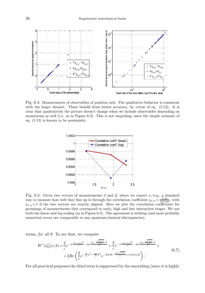
Fig. 6.4: Measurements of observables of position only. The qualitative behavior is consistentwith the larger dataset. These benefit from better accuracy, by virtue of eq. (5.12). It isclear that qualitatively the picture doesn’t change when we include observables depending onmomentum as well (i.e. as in Figure 6.3). This is not surprising, since the simple estimate ofeq. (5.13) is known to be pessimistic.
Fig. 6.5: Given two vectors of measurements ~x and ~y, where we expect xi≈yi, a standardway to measure how well they line up is through the correlation coefficient ρx,y =
〈~x,~y〉‖~x‖‖~y‖
, withρx,y=1 if the two vectors are exactly aligned. Here we plot the correlation coefficients forgroupings of measurements that correspond to early, high and late interaction stages. We useboth the linear and log scaling (as in Figure 6.3). The agreement is striking (and most probablynumerical errors are comparable to any quantum-classical discrepancies).
terms, for all θ. To see that, we compute
W ε[uε0](x,k)=
2
εe−π
(x−x0)2
ε−4π
(k−√
|x0|2π
)2
ε +2
εe−π
(x+x0)2
ε−4π
(k+
√|x0|2π
)2
ε +
+2Re
(2
εe−
πεx2− 4π
εk2
e−2πiθ− 2i√
|x0|ε
x+4πix0k
);
(6.7)
For all practical purposes the third term is suppressed by the smoothing (since it is highly
Athanassoulis, Katsaounis & Kyza 27
oscillatory), and with it all trace of θ in W ε[uε0]. The flow is also symmetric around
(0,0), hence one quickly observes that ρε(t) in this problem predicts a distribution ofmass symmetric around zero.
A crucial observable we study closely for this problem, is the amount of mass locatedto each side of x=0 after the crossing is completed,
∫±x>0
|uε0(x,t∗)|dx for t∗ sufficiently
large. An eventual mass imbalance means that there are interactions going on notincluded in the classical dynamics of (1.3).
The computational domain is taken sufficiently large to avoid possible interactionswith the boundary and we discretize in space using quintic B-splines. The initial con-dition is of the form
u0(x)=a0,1(x)eiS0,1(x)
ε +a0,2(x)eiS0,2(x)
ε ei2πθ, 0≤ θ≤ 1,
a0,1(x)= ε−14 e
−π2 (
x−x0√ε
)2, a0,2= ε−
14 e
−π2 (
x+x0√ε
)2,
S0,1(x)=√|x0|(x−x0), S0,2(x)=−
√|x0|(x+x0).
(6.8)
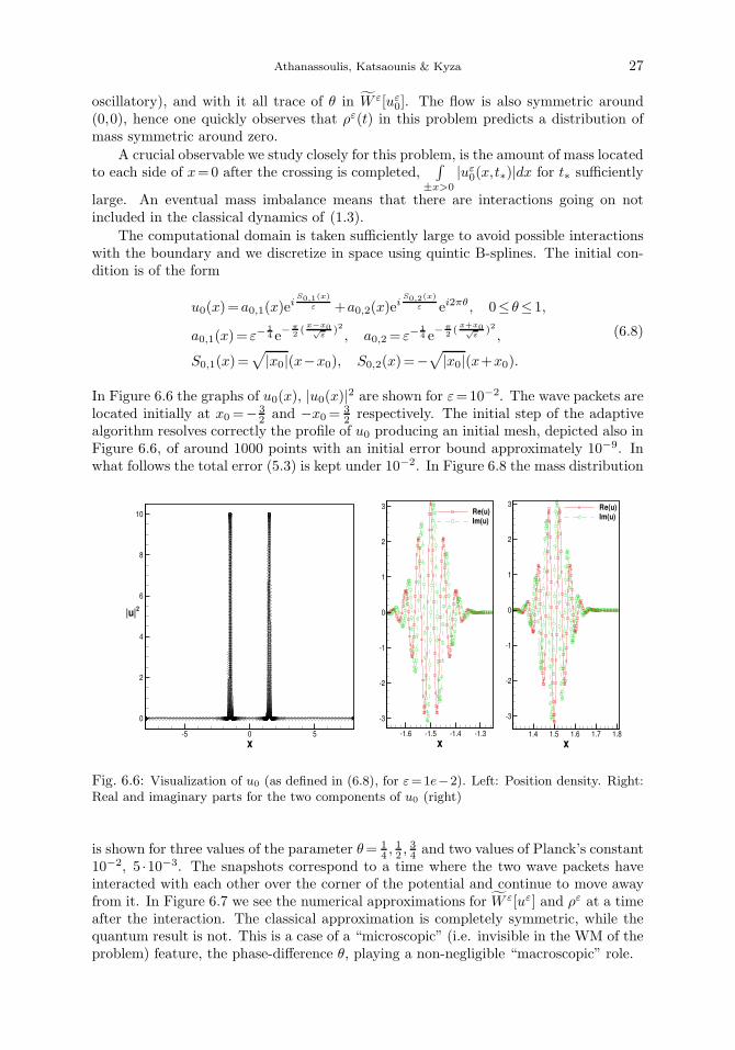
In Figure 6.6 the graphs of u0(x), |u0(x)|2 are shown for ε=10−2. The wave packets arelocated initially at x0=− 3
2 and −x0=32 respectively. The initial step of the adaptive
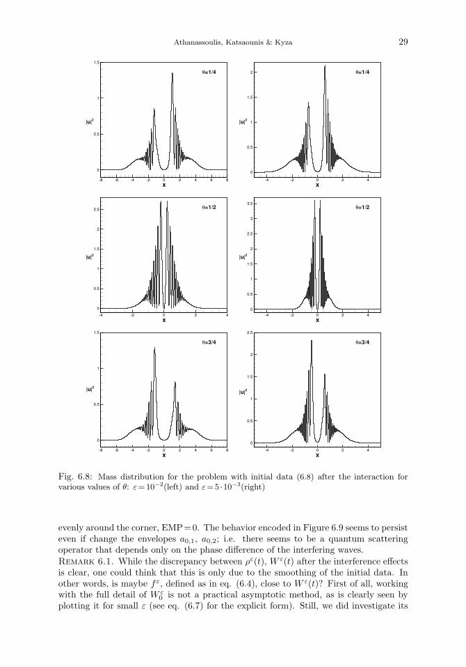
algorithm resolves correctly the profile of u0 producing an initial mesh, depicted also inFigure 6.6, of around 1000 points with an initial error bound approximately 10−9. Inwhat follows the total error (5.3) is kept under 10−2. In Figure 6.8 the mass distribution
x-5 0 5
0
2
4
6
8
10
|u|2
x1.4 1.5 1.6 1.7 1.8
-3
-2
-1
0
1
2
3 Re(u)
Im(u)
x-1.6 -1.5 -1.4 -1.3
-3
-2
-1
0
1
2
3Re(u)
Im(u)
Fig. 6.6: Visualization of u0 (as defined in (6.8), for ε=1e−2). Left: Position density. Right:Real and imaginary parts for the two components of u0 (right)
is shown for three values of the parameter θ= 14 ,
12 ,
34 and two values of Planck’s constant
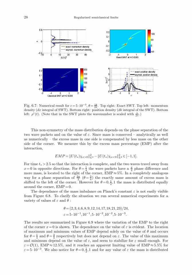
10−2, 5 ·10−3. The snapshots correspond to a time where the two wave packets haveinteracted with each other over the corner of the potential and continue to move awayfrom it. In Figure 6.7 we see the numerical approximations for W ε[uε] and ρε at a timeafter the interaction. The classical approximation is completely symmetric, while thequantum result is not. This is a case of a “microscopic” (i.e. invisible in the WM of theproblem) feature, the phase-difference θ, playing a non-negligible “macroscopic” role.
28 Regularized semiclassical limits
Fig. 6.7: Numerical result for ε=5 ·10−3, θ= 18
24. Top right: Exact SWT. Top left: momentum
density (dx integral of SWT). Bottom right: position density (dk integral of the SWT). Bottomleft: ρε(t). (Note that in the SWT plots the wavenumber is scaled with 1
2π.)
This non-symmetry of the mass distribution depends on the phase separation of thetwo wave packets and on the value of ε. Since mass is conserved – analytically as wellas numerically – the excess mass in one side is compensated by less mass on the otherside of the corner. We measure this by the excess mass percentage (EMP) after theinteraction,
EMP = ‖U(t∗)χx>0‖2L2 −‖U(t∗)χx<0‖2L2 ∈ [−1,1].
For time t∗> 2.5 so that the interaction is complete, and the two waves travel away fromx=0 in opposite directions. For θ= 1
4 the wave packets have a π2 phase difference and
more mass, is located to the right of the corner, EMP≈ 5%. In a completely analogousway for a phase separation of 3π
2 (θ= 34 ) the exactly same amount of excess mass is
shifted to the left of the corner. However for θ=0, 12 ,1 the mass is distributed equallyaround the corner, EMP=0.
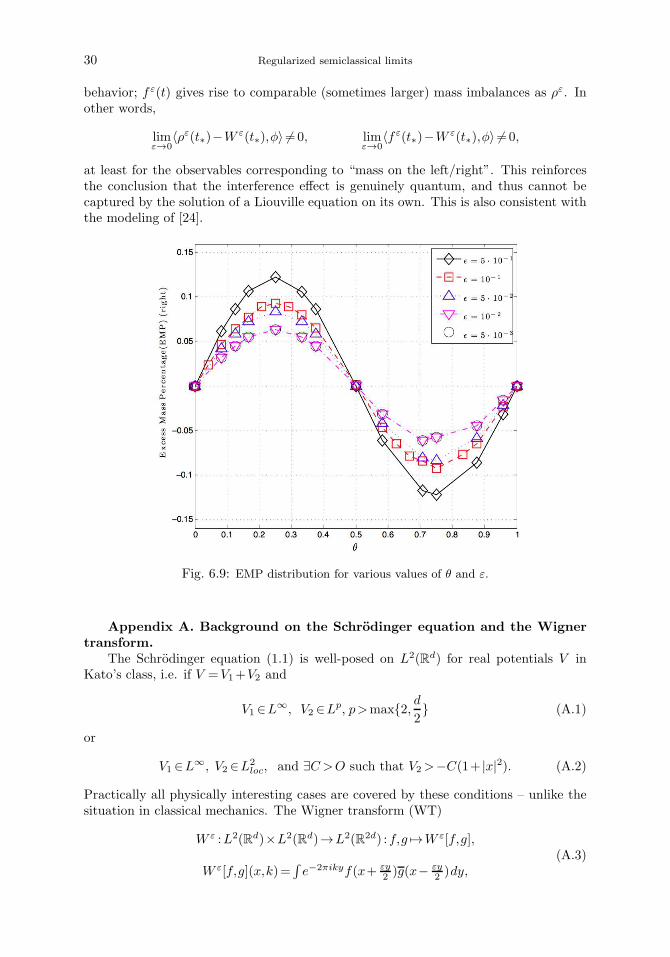
The dependance of the mass imbalance on Planck’s constant ε is not easily visiblefrom Figure 6.8. To clarify the situation we run several numerical experiments for avariety of values of ε and θ :
θ=(2,3,4,6,8,9,12,14,17,18,21,23)/24,
ε=5 ·10−1,10−1,5 ·10−2,10−2,5 ·10−3.
The results are summarized in Figure 6.9 where the variation of the EMP to the rightof the corner x=0 is shown. The dependence on the value of ε is evident. The locationof maximum and minimum values of EMP depend solely on the value of θ and occursfor θ= 1
4 and θ= 34 respectively but does not depend on ε. The value of this maximum
and minimum depend on the value of ε, and seem to stabilize for ε small enough. Forε=O(1), EMP≈ 12.5%, and it reaches an apparent limiting value of EMP≈ 5.5% forε=5 ·10−3. We also notice for θ=0, 12 ,1 and for any value of ε the mass is distributed
Athanassoulis, Katsaounis & Kyza 29
x-8 -6 -4 -2 0 2 4 6 8
0
0.5
1
1.5
θ=1/4
|u|2
x-4 -2 0 2 4
0
0.5
1
1.5
2 θ=1/4
|u|2
x-4 -2 0 2 4
0
0.5
1
1.5
2
2.5θ=1/2
|u|2
x-4 -2 0 2 4
0
0.5
1
1.5
2
2.5
3
3.5
θ=1/2
|u|2
x-8 -6 -4 -2 0 2 4 6 8
0
0.5
1
1.5
θ=3/4
|u|2
x-4 -2 0 2 4
0
0.5
1
1.5
2
2.5
θ=3/4
|u|2
Fig. 6.8: Mass distribution for the problem with initial data (6.8) after the interaction forvarious values of θ: ε=10−2(left) and ε=5 ·10−3(right)
evenly around the corner, EMP=0. The behavior encoded in Figure 6.9 seems to persisteven if change the envelopes a0,1, a0,2; i.e. there seems to be a quantum scatteringoperator that depends only on the phase difference of the interfering waves.
Remark 6.1. While the discrepancy between ρε(t), W ε(t) after the interference effectsis clear, one could think that this is only due to the smoothing of the initial data. Inother words, is maybe f ε, defined as in eq. (6.4), close to W ε(t)? First of all, workingwith the full detail of W ε
0 is not a practical asymptotic method, as is clearly seen byplotting it for small ε (see eq. (6.7) for the explicit form). Still, we did investigate its
30 Regularized semiclassical limits
behavior; f ε(t) gives rise to comparable (sometimes larger) mass imbalances as ρε. Inother words,
limε→0
〈ρε(t∗)−W ε(t∗),φ〉 6=0, limε→0
〈f ε(t∗)−W ε(t∗),φ〉 6=0,
at least for the observables corresponding to “mass on the left/right”. This reinforcesthe conclusion that the interference effect is genuinely quantum, and thus cannot becaptured by the solution of a Liouville equation on its own. This is also consistent withthe modeling of [24].
Fig. 6.9: EMP distribution for various values of θ and ε.
Appendix A. Background on the Schrodinger equation and the Wigner
transform.
The Schrodinger equation (1.1) is well-posed on L2(Rd) for real potentials V inKato’s class, i.e. if V =V1+V2 and
V1∈L∞, V2 ∈Lp, p>max2, d2 (A.1)
or
V1∈L∞, V2∈L2loc, and ∃C>O such that V2>−C(1+ |x|2). (A.2)
Practically all physically interesting cases are covered by these conditions – unlike thesituation in classical mechanics. The Wigner transform (WT)
W ε :L2(Rd)×L2(Rd)→L2(R2d) :f,g 7→W ε[f,g],
W ε[f,g](x,k)=∫e−2πikyf(x+ εy
2 )g(x− εy2 )dy,
(A.3)
Athanassoulis, Katsaounis & Kyza 31
seen as a bilinear mapping is essentially unitary in L2, in the sense that
‖W ε[f,g]‖L2(R2d)= ε−d2 ‖f‖L2(Rd)‖g‖L2(Rd). (A.4)
This allows the construction of an L2 propagator for the Wigner equation out of theSchrodinger propagator [32]. We would like to interpret the WT as a phase-spaceprobability density in the sense of classical statistical mechanics; it has e.g. the correctmarginals as position and momentum density
∫W ε[f ](x,k)dk= |f(x)|2,
∫W ε[f ](x,k)dx= |f(x)|2. (A.5)
However this picture cannot be taken too literally, since the WT has negative values ingeneral [12, 23]. In fact, it has been realized that when smoothed with an appropriatelylarge kernel, the WT becomes non-negative. Skipping over some details, this can beseen as an equivalent reformulation of the Heisenberg uncertainty principle: one canget a valid (i.e. a priori non-negative) probability that a particle occupies a regionin phase-space only if that region is large enough. This leads to the definition of theHusimi transform,
Hε[f ](x,k)=
(2
ε
)d
e−2πε [|x|
2+|k|2] ∗W ε[f ]> 0 ∀f ∈L2. (A.6)
The Husimi transform is used to prove the positivity of the WM, since, as can be readilychecked, W ε[uε] and Hε[uε] are close in weak sense as ε0 [30].
The particular topology used for weak-∗ convergence W ε[uε],Hε[uε]W 0 is builton the algebra of test functions A, introduced in [30] and defined as
A= φ∈C(R2d)|∫
supx
|FkK [φ(x,k)]|dK <∞. (A.7)
The main result for Wigner measures in smooth problems, precisely stated, is the fol-lowing
Theorem A.1 (Wigner Measures for the linear Schrodinger equation [30, 21]). Letthe real valued potential V be in Kato’s class, and assume there exists a C> 0 suchthat V (x)>−C(1+ |x|2). Assume moreover that the family of initial data uεn
0 , for asequence lim
n→∞εn=0, has the following properties
• (ε-oscillation) If Fφ(R) is defined as
Fφ(R)= limsupn→∞
∫
|k|> Rεn
|φuεn0 |2dk,
then, for all continuous, compactly supported φ
limR→∞
Fφ(R)=0.
• (compactness) If G(R) is defined by
G(R)= limsupn→∞
∫
|x|>R
|uεn0 |2dx,
then
limR→∞
G(R)=0.
32 Regularized semiclassical limits
Then, for a semiclassical family of problems of the form (1.1), and any timescaleT > 0, the following hold:
• There exists a subsequence of the initial data, uεmn
0 , so that their Wigner trans-form converges in A′ weak-∗ sense to a probability measure,
∀φ∈A limn→∞
〈W εmn
0 −W 00 ,φ〉=0, W 0
0 ∈M1+(R
2d)
• For t∈ [0,T ], define W 0(t) as the propagation of the initial Wigner measure W 00
under the Liouville equation (2.5). Then
W ε[uεn(t)]=W εn(t)W 0(t)
in A′ weak-∗ sense.
Finally, one should note that if f,g are “nice enough”, then their WT W ε[f,g] willalso be “nice”:Definition A.2. Σm We will say that f ∈L2(Rd) belongs to Σm if
‖f‖Σm = max|a|,|b|6m
‖xa∂bxf‖L2 <+∞.
Remark: It is clear that f ∈Σm⇒ f ∈Σm.Theorem A.3. If f,g∈Σm(Rd) (see Definition A.2 above), then
W ε[f,g]∈Σm(R2d). (A.8)
Moreover,
if m> 2d, then W ε[f,g]∈L1∩L∞. (A.9)
Proof: Observe that if
R :F (x,y) 7→F (x+Cy,x−Cy),
the Wigner transform can be seen just as a composition of
W ε[f,g]=Fy→kR ε2f(x)g(y).
So the strategy for the proof of (A.8) is clear; show that f(x)g(y)∈Σm(R2d), andthen show that each of the operators RC , Fy→k are bounded on Σm(R2d).
So, if f,g∈Σm(Rd), it readily follows that
‖f(x)g(y)‖Σm(R2d)= max|a1|+|a2|,|b1|+|b2|6m
‖xa1ya2∂b1x ∂b2
y f(x)g(y)‖L2 6
6 max|a1|,|b1|6m
‖xa1∂b1x f(x)‖L2 max
|a2|,|b2|6m‖ya2∂b2
y g(y)‖L2 6 ‖f‖Σm(Rd)‖g‖Σm(Rd).
Now assume F (x,y)∈Σm(R2d);
‖RCF‖Σm(R2d)6 max|a1|+|a2|,|b1|+|b2|6m
‖xa1ya2∂b1x ∂b2
y F (x+Cy,x−Cy)‖L2 =
= max|a1|+|a2|,|b1|+|b2|6m
‖(
x+Cy+ (x−Cy)2
)a1(
x+Cy− (x−Cy)C
)a2
∂b1x ∂b2
y F (x+Cy,x−Cy)‖L2 6
6C′‖F‖Σm(R2d).
Athanassoulis, Katsaounis & Kyza 33
Finally
‖Fy→kF‖Σm(R2d)6 max|a1|+|a2|,|b1|+|b2|6m
‖xa1ka2∂b1x ∂b2
k F2(x,k)‖L2 =
6 max|a1|+|a2|,|b1|+|b2|6m
(2π)b2−a2‖xa1∂b1x ∂a2
y
(yb2F (x,y)
)‖L2 6C′′‖F‖Σm(R2d).
Now to prove (A.9); by virtue of the Sobolev embedding Theorem [15]
‖F‖L∞(R2d)6 ‖F‖Hd+1(R2d)6 ‖F‖Σd+1(R2d);
moreover
‖F‖L1(R2d)=∫x,y
|F (x,y)|dxdy=∫x,y
|F (x,y)| (1+|x|2+|y|2)r(1+|x|2+|y|2)r dxdy6
6 ‖(1+ |x|2+ |y|2)rF (x,y)‖L2(R2d)‖ 1(1+|x|2+|y|2)r ‖L2(R2d)6 ‖F‖Σ4r(R2d)
√∞∫
ρ=0
ρ2d−1dρ(1+ρ2)2r
which is finite for r> d2 .
Appendix B. The Smoothed Wigner Transform.
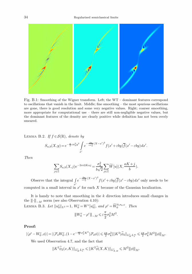
As was mentioned, sometimes flexibility in the calibration of the smoothing is re-quired. Several approaches for the smoothing of the Wigner transform have been studied[12, 23], and there exist trade offs for the different choices and scalings of smoothingkernels. We use a Gaussian smoothing in what we call the Smoothed Wigner transform(SWT). This has the advantage that it leads to entire analytic functions of known orderand type, thus making available a great toolbox of results for their asymptotic study[7].
The SWT was introduced in (2.8). Observe that
W ε[u](x,k)=
(2
εσxσk
)d ∫
x,k
e− 2π
ε
[
|x−x′|2σ2x
+ |k−k′|2σ2k
]
W ε(x′,k′)dx′dk′=
=
( √2√
εσx
)d∫
y
e−2πiky− επ2 σ2
ky2
∫
x′
e− 2π
ε
|x−x′|2σ2x u(x′+
yε
2)u(x′− yε
2)dx′dy,
(B.1)therefore only d convolutions are needed (i.e. in x), as the smoothing in k can beperformed as part of the FFT.
To implement this transform numerically, we will use the FFT. First of all recallthatLemma B.1. For any function f ∈S(R),
∑
j∈Z
f(jh)e−2πiknh=1
h
∑
j∈Z
f(k+j
h).
This is a direct corollary of the Poisson summation formula, and the starting pointof any use of the FFT to approximate the Fourier transform of a continuous function.(The requirement f ∈S(R) can be relaxed; the details along this direction are outsidethe scope of this work.)
Similarly, we can create an appropriate version of the Poisson summation formulafor the evaluation of the dy integral in (B.1) as an FFT:
34 Regularized semiclassical limits
Fig. B.1: Smoothing of the Wigner transform. Left; the WT – dominant features correspondto oscillations that vanish in the limit. Middle; fine smoothing – the most spurious oscillationsare gone, there is good resolution and some very negative values. Right; coarser smoothing,more appropriate for computational use – there are still non-negligible negative values, butthe dominant features of the density are clearly positive while definition has not been overlysmeared.
Lemma B.2. If f ∈S(R), denote by
Sa,b(X,y)= e−π2 εσ2
ky2
∫
x′
e− 2π
εσ2x(X−x′)2
f(x′+εby)f(x′−εby)dx′.
Then
∑
j∈Z
Sa,b(X,j)e−2πi2Kaj =σ2k
b√2
∑
j∈Z
W [u](X,aK+j
b).
Observe that the integral∫x′e− 2π
εσ2x(X−x′)2
f(x′+εby)f(x′−εby)dx′ only needs to be
computed in a small interval in x′ for each X because of the Gaussian localization.
It is handy to note that smoothing in the k direction introduces small changes inthe |||·|||−M norm (see also Observation 4.10):
Lemma B.3. Let ‖uε0‖L2 =1, W ε
0 =W ε[uε0], and ρε= W 0,σk;ε
0 . Then
|||W ε0 −ρε|||−M 6 ε
π
2σ2kM
2.
Proof:
|〈ρε−W ε0 ,φ〉|= |〈F2W
ε0 ,(1−e−
επ2 σ2
kK2
)F2φ〉|6 επ2 σ2
k‖|K2|φ2‖L1KL∞
x6 επ
2 σ2kM
2|||φ|||M .
We used Observation 4.7, and the fact that
‖K2φ2(x,K)‖L1KL∞
x6 ‖K2φ(X,K)‖L1
X,K6M2|||φ|||M .
Athanassoulis, Katsaounis & Kyza 35
squareRemark: Observe that in practice
limε→0
〈W ε0 −W ε
0 ,φ〉=0
(which is significantly weaker than (4.13) or lemma B.3 above) is often sufficient inpractice. In particular, the use of some smoothing in the x direction as well, does notseem to hurt the quality of approximation in our numerical examples. In any case, wehave an explicit, uniform upper bound for the effect of smoothing in the k variablesonly.
Appendix C. Slicing in two of a WKB wavefunction.
A more singular non-interference problem example is given by the initial data
u0(x)=a0(x)eiS0(x)
ε ,
a0(x)= (1+ tanh(7(x+3))) ·(1+ tanh(7(−x+1))), S0(x)=−23 |x| 32
(C.1)
and
V (x)=1+(1+tanh(4(x+4)))(1+tanh(−4(x−4)))(−|x|+4)
8. (C.2)
The initial WM of this problem is a line supported measure. The concentrationlimit of ρε predicts that this measure would be “sliced” into two lines. We see clearqualitative agreement between ρε and W ε, see Figure C.1. The quantum observables(6.6) (including mass scattered to the left / right) are within around 4% of their semi-classical prediction. Overall it seems that quantitative convergence as ε→0 is takingplace, albeit somewhat more slowly for this type of initial data than for the data of eq.(6.5).
REFERENCES
[1] G. Akrivis, Ch. Makridakis, & R. H. Nochetto, A posteriori error estimates for the Crank-Nicolson
method for parabolic equations, Math. Comp., 75, pp. 511–531, 2006.[2] L. Ambrosio & A. Figalli, Almost everywhere well-posedness of continuity equations with measure
initial data, C. R. Math. Acad. Sci. Paris, 348, pp. 249–252, 2010.[3] L. Ambrosio, G. Friesecke & J. Giannoulis, Passage from Quantum to Classical Molecular Dy-
namics in the Presence of Coulomb Interactions, Comm. Part. Diff. Eq., 35, pp. 1490–1515,2010.
[4] L. Ambrosio, A. Figalli, G. Friesecke, J. Giannoulis & T. Paul, Semiclassical limit of quantum
dynamics with rough potentials and well posedness of transport equations with measure initial
data, Comm. Pure Appl. Math., 64-9, pp. 1199–1242, 2011.[5] A. Athanassoulis & T. Paul, Strong and weak semiclassical limits for some rough Hamiltonians,
Math. Mod. Meth. Appl. S., 12-22, p. 1250038, 2012.[6] A. Athanassoulis & T. Paul, On the selection of the classical limit for potentials with BV deriva-
tives, J. Dyn. Diff. Equat., 25-1, pp. 33–47, 2013.[7] A. Athanassoulis, N.J. Mauser & T. Paul, Coarse-scale representations and smoothed Wigner
transforms, J. Math. Pures Appl., 91-3, pp. 296–338, 2009.[8] A. Athanassoulis, Wigner measures for Schrodinger equations with weak power nonlinearities,
arXiv:1505.04707.[9] A. Bamberger, B. Engquist, L. Halpern & P. Joly, Higher order paraxial wave equation approxi-
mations in heterogeneous media, SIAM J. Appl. Math., 48-1, pp. 129 – 154, 1988.[10] W. Bao, S. Jin, & P.A. Markowich, Numerical study of time-splitting spectral discretizations of
nonlinear Schrodinger equations in the semiclassical regimes, SIAM J. Sci. Comput., 25-1,pp. 27–64, 2003.
[11] F. Bouchut, Renormalized solutions to the Vlasov equation with coefficients of bounded variation,Arch. Ration. Mech. Anal., 157-1, pp. 75–90, 2001.
36 Regularized semiclassical limits
[12] L. Cohen, Time frequency distributions - a review, Proc. IEEE, 77-7, pp. 941–981, 1989.[13] M. de Hoop, G. Hormann & M. Oberguggenberger, Evolution systems for paraxial wave equations
of Schrodinger-type with non-smooth coefficients, J. Diff. Eq., 245-6, pp. 1413–1432, 2008.[14] W. Dorfler, A time-and space-adaptive algorithm for the linear time-dependent Schrodinger equa-
tion, Numer. Math., 73, pp. 419–448, 1996.[15] L. C. Evans, Partial Differential Equations, 2nd edition, American Mathematical Society, 2010.[16] C. Fermanian Kammerer, P. Gerard A Landau-Zener formula for non-degenerated involutive
codimension 3 crossings, Ann. Henri Poincare, 4-3, pp. 513–552, 2003.[17] C. Fermanian-Kammerer, P. Gerard & C. Lasser, Wigner measure propagation and conical sin-
gularity for general initial data, Arch. Ration. Mech. Anal., 209-1, pp. 209–236, 2013.[18] G. Folland, Harmonic analysis in phase space, Princeton University Press, 1989.[19] I. M. Gelfand & G.E. Shilov, Generalized functions, vol. I Academic Press, 1964.[20] F. Golse, The mean-field limit for the dynamics of large particle systems, Journees equations aux
derivees partielles, pp. 1 – 47, 2003.[21] P. Gerard, P. Markowich, N. J. Mauser & F. Poupaud, Homogenization limits and Wigner trans-
forms, Comm. Pure Appl. Math., 50-4, pp. 323–379, 1997.[22] L. Harris, J. Lukkarinen, S. Teufel & F. Theil, Energy Transport by Acoustic Modes of Harmonic
Lattices, SIAM J. Math. Anal., 40-4, pp. 1392–1418, 2008.[23] F. Hlawatsch & G. F. Boudreaux-Bartels, Linear and quadratic time-frequency signal represen-
tations, IEEE Signal Proc. Mag., 9-2, pp. 21–67, 1992.[24] S. Jin & K. Novak, A coherent semiclassical transport model for pure-state quantum scattering,
Comm. Math. Sci., 8 pp. 253-275, 2010.[25] S. Jin P.A. Markowich & C. Sparber, Mathematical and Computational methods for semiclassical
Schrodinger equations, Acta Numer., 20, pp. 121–209, 2011.[26] Th. Katsaounis & I. Kyza, A posteriori error control and adaptivity for Crank-Nicolson finite
element approximations for the linear Schrdinger equation, Numer. Math. 129-1, pp. 55–90,2015.
[27] C. Lasser & S. Teufel, Propagation through conical crossings: An asymptotic semigroup, Comm.Pure Appl. Math., 58-9, pp. 1188–1230, 2005.
[28] M. Lax, W. H. Louisell & W. B. McKnight, From Maxwell to paraxial wave optics, Phys. Rev.A, 11-4, pp. 1365–1370, 1975.
[29] S. Leung, J. Qian & S. Osher, A level set method for three-dimensional paraxial geometrical optics
with multiple point sources, Commun. Math. Sci., 2-4, pp. 643–672, 2004.[30] P.L. Lions & T. Paul, Sur les mesures de Wigner, Rev. Mat. Iberoam., 9-3, pp. 553–618, 1993.[31] Ch. Makridakis, R.H. Nochetto, Elliptic reconstruction and a posteriori error estimates for
parabolic problems, SIAM J. Numer. Anal. 41, pp. 1585–1594, 2003.[32] P.A. Markowich & H.Neunzert, On the equivalence of the Schrodinger and the quantum Liouville
equations, Math. Methods Appl. Sci., 11-4, pp. 459–469, 1989.[33] A.A.M. Marte & S. Stenholm, Paraxial light and atom optics: the optical Schrodinger equation
and beyond, Phys. Rev. A, 56-4, pp. 2940–2953, 1997.[34] A. Mielke, Macroscopic behavior of microscopic oscillations in harmonic lattices via Wigner-
Husimi transforms, Arch. Ration. Mech. Anal., 181, pp. 401–448, 2006.[35] L. Miller, Refraction of high-frequency waves density by sharp interfaces and semiclassical mea-
sures at the boundary, J. Math. Pures Appl., 79-3, pp. 227–269, 2000.[36] O. Pinaud, Classical limit for a system of random non-linear Schrodinger equations Arch. Ration.
Mech. Anal., 209-1, pp. 321-364, 2013.[37] L. Ryzhik , G. Papanicolaou & J. B. Keller, Transport equations for elastic and other waves in
random media, Wave Motion, 24, p. 327–370, 1996.[38] S. Teufel, Adiabatic Perturbation Theory in Quantum Dynamics, Springer, 2003.[39] H. Waalkens, R. Schubert & S. Wiggins, Wigner’s dynamical transition state theory in phase
space: classical and quantum, Nonlinearity, 21-1, 2008.
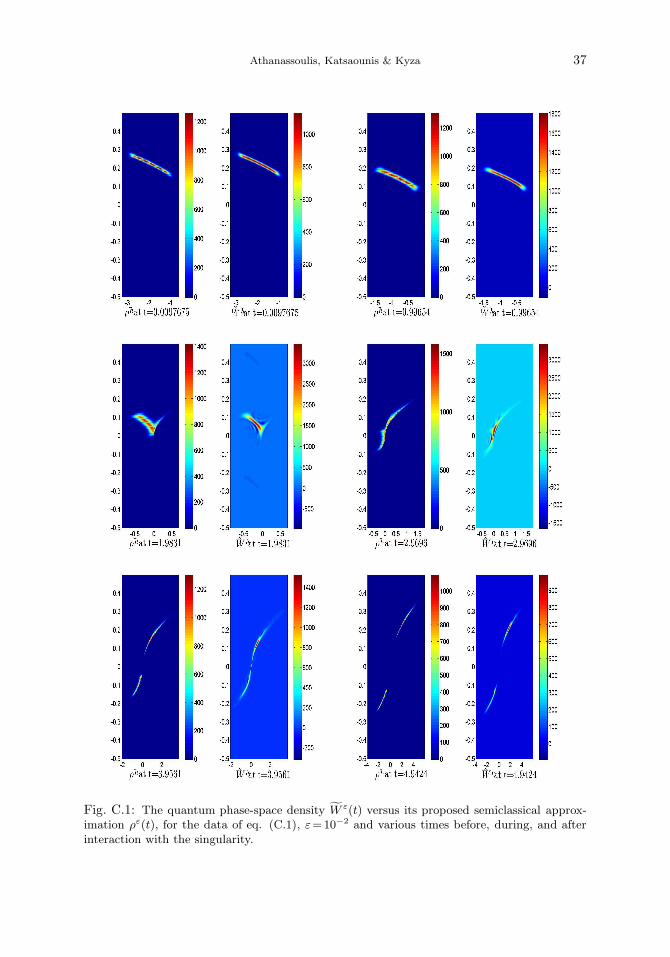
Athanassoulis, Katsaounis & Kyza 37
Fig. C.1: The quantum phase-space density W ε(t) versus its proposed semiclassical approx-imation ρε(t), for the data of eq. (C.1), ε=10−2 and various times before, during, and afterinteraction with the singularity.