university of reginastat.math.uregina.ca/~kozdron/teaching/regina/851winter08/handouts/... ·...
TRANSCRIPT

University of Regina
Statistics 851 – Probability
Lecture Notes
Winter 2008
Michael Kozdron
http://stat.math.uregina.ca/∼kozdron
References
[1] Jean Jacod and Philip Protter. Probability Essentials, second edition. Springer, Heidel-berg, Germany, 2004.
[2] Jeffrey S. Rosenthal. A First Look at Rigorous Probability Theory. World Scientific,Singapore, 2000.

Preface
Statistics 851 is the first graduate course in measure-theoretic probability at the Universityof Regina. There are no formal prerequisites other than graduate student status, althoughit is expected that students encountered basic probability concepts such as discrete andcontinuous random variables at some point in their undergraduate careers. It is also expectedthat students are familiar with some basic ideas of set theory including proof by inductionand countability.
The primary textbook for the course is [1] and references to chapter, theorem, and exercisenumbers are for that book. Lectures #1 and #9, however, are based on [2] which is one ofthe supplemental course books.
These notes are for the exclusive use of students attending the Statistics 851 lectures andmay not be reproduced or retransmitted in any form.
Michael KozdronRegina, SKJanuary 2008
List of Lectures and Handouts
Lecture #1: The Need for Measure Theory
Lecture #2: Introduction
Lecture #3: Axioms of Probability
Lecture #4: Definition of Probability Measure
Lecture #5: Conditional Probability
Lecture #6: Probability on a Countable Space
Lecture #7: Random Variables on a Countable Space
Lecture #8: Expectation of Random Variables on a Countable Space
Lecture #9: A Non-Measurable Set
Lecture #10: Construction of a Probability Measure
Lecture #11: Null Sets
Lecture #12: Random Variables
Lecture #13: Random Variables
Lecture #14: Some General Function Theory
Lecture #15: Expectation of a Simple Random Variable
Lecture #16: Integration and Expectation
Handout: Interchanging Limits and Integration
Lecture #17: Comparison of Lebesgue and Riemann Integrals
Lecture #18: An Example of a Random Variable with a Non-Borel Range
Lecture #19: Construction of Expectation
Lecture #20: Independence
Lecture #21: Product Spaces
Handout: Exercises on Independence
Handout: Exercises on Independence (Solutions)
Lecture #22: Product Spaces
Lecture #23: The Fubini-Tonelli Theorem
Lecture #24: The Borel-Cantelli Lemma
Lecture #25: Midterm Review
Lecture #26: Convergence Almost Surely and Convergence in Probability
Lecture #27: Convergence of Random Variables
Lecture #28: Convergence of Random Variables
Lecture #29: Weak Convergence

Lecture #30: Weak Convergence
Lecture #31: Characteristic Functions
Lecture #32: The Primary Limit Theorems
Lecture #33: Further Results on Characteristic Functions
Lecture #34: Conditional Expectation
Lecture #35: Conditional Expectation
Lecture #36: Introduction to Martingales

Statistics 851 (Winter 2008) January 7, 2008Prof. Michael Kozdron
Lecture #1: The Need for Measure Theory
Reference. Today’s notes and §1.1 of [2]
In order to study probability theory in a mathematically rigorous way, it is necessary tolearn the appropriate language which is “measure theory.”
Theoretical probability is used in a variety of diverse fields such as
• statistics,
• economics,
• management,
• finance,
• computer science,
• engineering,
• operations research.
More will be said about the applications as the course progresses.
For now, however, we will begin with some “easy” examples from undergraduate probability(STAT 251/STAT 351).
Example. Let X be a Poisson(5) random variable. What does this mean?
Solution. It means that X takes on a “random” non-negative integer k (k ≥ 0) accordingto the probability mass fuction
fX(k) := PX = k =e−55k
k!, k ≥ 0.
We can then compute things like the expected value of X2, i.e.,
E(X2) =∞∑
k=0
k2PX = k =∞∑
k=0
k2e−55k
k!.
Note that X is an example of a discrete random variable.
Example. Let Y be a Normal(0, 1) random variable. What does this mean?
1–1
Solution. It means that the probability that Y lies between two real numbers a and b (witha ≤ b) is given by
Pa ≤ Y ≤ b =
∫ b
a
1√2π
e−y2/2 dy.
Of course, for any real number y, we have PY = y = 0. (How come?) We say that theprobability density function for Y is
fY (y) =1√2π
e−y2/2, −∞ < y < ∞.
We can then compute things like the expected value of Y 2, i.e.,
E(Y 2) =
∫ ∞
−∞y2 1√
2πe−y2/2 dy.
Note that Y is an example of a (absolutely) continuous random variable.
Example. Introduce a new random variable Z as follows. Flip a fair coin (independently),and set Z = X if it comes up heads and set Z = Y if it comes up tails. That is,
PZ = X = PZ = Y = 1/2.
What kind of random variable is Z?
Solution. We can formally define Z to be the random variable
Z = XW + Y (1−W )
where the random variable W satisfies
PW = 1 = PW = 0 = 1/2
and is independent of X and Y . Clearly Z is not discrete since it can take on uncountablymany values, and it is not absolutely continuous since PZ = z > 0 for certain values of z(namely when z is a non-negative integer).
Question. How do we study Z? How could you compute things like E(Z2)? (Hint: If youtried to compute E(Z2) using undergraduate probability then you would be conditioning onan event of probability 0. That is not allowed.)
Answer. The distinction between discrete and absolutely continuous is artificial. Measuretheory gives a common definition to expected value which applies equally well to discreterandom variables (like X), absolutely continuous random variables (like Y ), combinations(like Z), and ones not yet imagined.
1–2

Statistics 851 (Winter 2008) January 9, 2008Prof. Michael Kozdron
Lecture #2: Introduction
Reference. Chapter 1 pages 1–5
Intuitively, a probability is a measure of the likelihood of an event.
Example. There is a 60% chance of snow tomorrow:
Psnow tomorrow = 0.60.
Example. There is a probability of 1/2 that this coin will land heads:
Pheads = 0.50.
The method of assigning probabilities to events is a philosophical question.
• What does it mean for there to be a 60% chance of snow tomorrow?
• What does it mean for a fair coin to have a 50% chance of landing heads?
There are roughly two paradigms for assigning probabilities. One is the frequentist approachand the other is the Bayesian approach.
The frequentist approach is based on repeated experimentation and long-run averages. If weflip a coin many, many times, we expect to see a head about half the time. Therefore, weconclude that the probability of heads on a single toss is 0.50.
In contrast, we cannot repeat “tomorrow.” There will only be one January 10, 2008. Eitherit will snow or it will not. The weather forecaster can predict snow with probability 0.60based on weather patterns, historical data, and intuition. This is a Bayesian, or subjectivist,approach to assigning probabilities.
Instead of entering into a philosophical discussion, we will assume that we have a reasonableway of assigning probabilities to events—either frequentist, Bayesian, or a combination ofthe two.
Question. What are some properties that a probability must have?
Answer. Assign a number between 0 and 1 to each event.
• The impossible event will have probability 0.
• The certain event will have probability 1.
• All events will have probability between 0 and 1. That is, if A is an event, then0 ≤ PA ≤ 1.
2–1

However, an event is not the most basic outcome of an experiment. An event may be acollection of outcomes.
Example. Roll a fair die. Let A be the event that an even number is rolled; that is,A = even number = 2 or 4 or 6. Intuitively, PA = 3/6.
Notation. Let Ω denote the set of all possible outcomes of an experiment. We call Ω thesample space which is composed of all individual outcomes. These are labelled by ω so thatΩ = ω ∈ Ω.
Example. Model the experiment of rolling a fair die.
Solution. The sample space is Ω = 1, 2, 3, 4, 5, 6. The individual outcomes ωi = i, i =1, 2, . . . , 6, are all equally likely so that
Pωi =1
6.
Definition. An event is a collection of outcomes. Formally, an event A is a subset of thesample space; that is, A ⊆ Ω.
Technical Matter. It will not be as easy as declaring all events as simply all possiblysubsets of Ω. (The set of all subsets of Ω is called the power set of Ω and denoted by 2Ω.) IfΩ is uncountable, then the power set will be too big!
Example. Model the experiment of flipping a fair coin. Include a list of all possible events.
Solution. The sample space is Ω = H, T. The list of all possible events is
∅, Ω, H, T.
Note that if we write A to denote the set of all possible events, then
A = ∅, Ω, H, T
satisfies |A| = 2|Ω| = 22 = 4. Since the individual outcomes are each equally likely we canassign probabilities to events as
P∅ = 0, PΩ = 1, PH = PT =1
2.
Instead of worrying about this technical matter right now, we will first study countablespaces. The collection A in the previous example has a special name.
Definition. A collection A of subsets Ai ⊆ Ω is called a σ-algebra if
(i) ∅ ∈ A,
(ii) Ω ∈ A,
(iii) A ∈ A implies Ac ∈ A, and
2–2
(iv) A1, A2, A3, . . . ∈ A implies∞⋃i=1
Ai ∈ A.
Remark. Condition (iv) is called countable additivity.
Example. A = ∅, Ω is a σ-algebra (called the trivial σ-algebra).
Example. For any subset A ⊂ Ω,
A = ∅, A,Ac, Ω
is a σ-algebra.
Example. If Ω is any space (whether countable or uncountable), then the power set of Ω isa σ-algebra.
Proposition. Suppose that A is a σ-algebra. If A1, A2, A3, . . . ∈ A, then
(v) A1 ∪ A2 ∪ · · · ∪ An ∈ A for every n < ∞, and
(vi)∞⋂i=1
Ai ∈ A.
Remark. Condition (v) is called finite additivity.
Proof. To show that finite additivity (v) follows from countable additivity simply take Ai,i > n, to be ∅. That is,
A1 ∪ A2 ∪ · · · ∪ An ∪ ∅ ∪ ∅ ∪ · · · =n⋃
i=1
Ai ∈ A
since A1, A2, . . . , An, ∅ ∈ A. Condition (vi) follows from De Morgan’s law (Exercise 2.3).Suppose that A1, A2, . . . ∈ A so that Ac
1, Ac2, . . . ∈ A by (iii). By countably additivity, we
have∞⋃i=1
Aci ∈ A.
Thus, by (iii) again we have [∞⋃i=1
Aci
]c
∈ A.
However, [∞⋃i=1
Aci
]c
=∞⋂i=1
[Aci ]
c =∞⋂i=1
Ai
which establishes (vi).
2–3
Definition. A collection A of events satisfying (i), (ii), (iii), (v) (but not (iv)) is called analgebra.
Remark. Some people say σ-field/field instead of σ-algebra/algebra.
Proposition. Suppose that A is a σ-algebra. If A1, A2, A3, . . . ∈ A, then
(vii) A1 ∩ A2 ∩ · · · ∩ An ∈ A for every n < ∞.
Proof. To show that this result follows from (vi) simply simply take Ai, i > n, to be Ω. Thatis,
A1 ∩ A2 ∩ · · · ∩ An ∩ Ω ∩ Ω ∩ · · · =n⋂
i=1
Ai ∈ A
since A1, A2, . . . , An, Ω ∈ A.
Definition. A probability (measure) is a set function P : A → [0, 1] satisfying
(i) P∅ = 0, PΩ = 1, and 0 ≤ PA ≤ 1 for every A ∈ A, and
(ii) if A1, A2, . . . ∈ A are disjoint, then
P
∞⋃i=1
Ai
=
∞∑i=1
PAi.
Definition. A probability space is a triple (Ω,A, P ) where Ω is a sample space, A is aσ-algebra of subsets of Ω, and P is a probability measure.
Example. Consider the experiment of tossing a fair coin twice. In this case,
Ω = HH,HT, TH, TT
and A consists of the |A| = 2|Ω| = 24 = 16 elements
A =
∅, Ω, HH, HT, TH, TT, HH,HT, HH,TH, HH,TT, HT, TH, HT, TT,
TH, TT, HH,HT, TH, HH,HT, TT, HH,TH, TT, HT, TH, TT
.
Example. Consider the experiment of rolling a fair die so that Ω = 1, 2, 3, 4, 5, 6. In thiscase, A consists of the 26 = 64 events
A = ∅, Ω, 1, 2, 3, 4, 5, 6, 12, 13, 14, 15, 16, 21, etc. .
We can then define
PA =|A|6
for every A ∈ A. (∗)
2–4

For instance, if A is the event roll even number = 2, 4, 6 and if B is the event roll oddnumber less than 4 = 1, 3, then
PA =3
6and PB =
2
6.
Furthermore, since A and B are disjoint (that is, A ∩B = ∅) we can use finite additivity toconclude
PA ∪B = PA+ PB =5
6. (∗∗)
Since A ∪B = 1, 2, 3, 4, 6 ∈ A has cardinality |A ∪B| = 5, we see that from (∗) that
PA ∪B =|A ∪B|
6=
5
6
which is consistent with (∗∗).
2–5

Statistics 851 (Winter 2008) January 11, 2008Prof. Michael Kozdron
Lecture #3: Axioms of Probability
Reference. Chapter 2 pages 7–11
Example. Construct a probability space to model the experiment of tossing a fair cointwice.
Solution. We must carefully define (Ω,A, P ). Thus, we take our sample space to be
Ω = HH,HT, TH, TT
and our σ-algebra A consists of the |A| = 2|Ω| = 24 = 16 elements
A =
∅, Ω, HH, HT, TH, TT, HH,HT, HH,TH, HH,TT, HT, TH, HT, TT,
TH, TT, HH,HT, TH, HH,HT, TT, HH,TH, TT, HT, TH, TT
.
In general, if Ω is finite, then the power set A = 2Ω (i.e., the set of all subsets of Ω) is aσ-algebra with |A| = 2|Ω|. We take as our probability a set function P : A → [0, 1] satisfyingcertain conditions. Thus,
P∅ = 0, PΩ = 1,
PHH = PTT = PHT = PTH =1
4,
PHH,HT = PHH,TH = PHH,TT = PHT, TH = PHT, TT = PTH, TT =1
2,
PHH,HT, TH = PHH,HT, TT = PHH,TH, TT = PHT, TH, TT =3
4.
That is, if A ∈ A, let
PA =|A|4
.
Random Variables
Definition. A function X : Ω → R given by ω 7→ X(ω) is called a random variable.
Remark. A random variable is NOT a variable in the algebraic sense. It is a function inthe calculus sense.
Remark. When Ω is more complicated than just a finite sample space we will need to bemore careful with this definition. For now, however, it will be fine.
3–1

Example. Consider the experiment of tossing a fair coin twice. Let the random variableX denote the number of heads. In order to define the function X : Ω → R we must defineX(ω) for every ω ∈ Ω. Thus,
X(HH) = 2, X(HT ) = 1, X(TH) = 1, X(TT ) = 0.
Note. Every random variable X on a probability space (Ω,A, P ) induces a probabilitymeasure on R which is denoted PX and called the law (or distribution) of X. It is definedfor every B ∈ B by
PX(B) := Pω ∈ Ω : X(ω) ∈ B = PX ∈ B = PX−1(B).
In other words, the random variable X transforms the probability space (Ω,A, P ) into theprobability space (R,B, PX):
(Ω,A, P )X−→ (R,B, PX).
The σ-algebra B is called the Borel σ-algebra on R. We will discuss this in detail shortly.
Example. Toss a coin twice and let X denote the number of heads observed. The law of Xis defined by
PX(B) =#(i, j) such that 1i = H+ 1j = H ∈ B
4
where 1 denotes the indicator function (defined below). For instance,
PX(2) = Pω ∈ Ω : X(ω) = 2 = PX = 2 = PHH =1
4,
PX(1) = PX = 1 = PHT, TH =1
2,
PX(0) = PX = 0 = PTT =1
4,
and
PX
([−1
2,3
2
])= P
ω ∈ Ω : X(ω) ∈
[−1
2,3
2
]= P
−1
2≤ X ≤ 3
2
= PX = 0 or X = 1
= PTT, HT, TH =3
4.
Later we will see how PX will be related to FX , the distribution function of X.
Notation. The indicator function of the event A is defined by
1A(x) = 1x ∈ A =
1, if x ∈ A,
0, if x 6∈ A.
Note. On page 5, it should read: “(for example, PX(2) = P (1, 1) = 136
. . .”
3–2
Definition. If C ⊆ 2Ω, then the σ-algebra generated by C is the smallest σ-algebra containingC. It is denoted by σ(C).
Note. By Exercise 2.1, the power set 2Ω is a σ-algebra. By Exercise 2.2, the intersection ofσ-algebras is itself a σ-algebra. Therefore, σ(C) always exists and
C ⊆ σ(C) ⊆ 2Ω.
Definition. The Borel σ-algebra on R, written B, is the σ-algebra generated by the opensets. (Equivalently, B is generated by the closed sets.) That is, if C denotes the collection ofall open sets in R, then B = σ(C).
In fact, to understand B it is enough to consider intervals of the form (−∞, a] as the nexttheorem shows.
Theorem. The Borel σ-algebra B is generated by intervals of the form (−∞, a] where a ∈ Qis a rational number.
Proof. Let C denote the collection of all open intervals. Since every open set in R is acountable union of open intervals, we must have σ(C) = B. Let D denote the collection ofall intervals of the form (−∞, a], a ∈ Q. Let (a, b) ∈ C for some b > a with b ∈ Q. Let
an = a +1
n
so that an ↓ a as n →∞, and let
bn = b +1
nso that bn ↑ b as n →∞. Thus,
(a, b) =∞⋃
n=1
(an, bn] =∞⋃
n=1
(−∞, bn] ∩ (−∞, an]c
which implies that (a, b) ∈ σ(D). That is, C ⊆ σ(D) so that σ(C) ⊆ σ(D). However, everyelement of D is a closed set which implies that
σ(D) ⊆ B.
This gives the chain of containments
B = σ(C) ⊆ σ(D) ⊆ B
and so σ(D) = B proving the theorem.
Remark. Exercises 2.9, 2.10, 2.11, 2.12 can be proved using Definition 2.3. For instance,since A∪Ac = Ω and A∩Ac = ∅, we can use use countable additivity (axiom 2) to conclude
PΩ = PA ∪ Ac = PA+ PAc.
We now use axiom 1, the fact that PΩ = 1, to find
1 = PA+ PAc and so PAc = 1− PA.
3–3
Proposition. If A ⊆ B, then PA ≤ PB.
Proof. We writeB = (A ∩B) ∪ (Ac ∩B) = A ∪ (Ac ∩B)
and note that(A ∩B) ∩ (Ac ∩B) = ∅.
Thus, by countable additivity (axiom 2) we conclude
PB = PA+ PAc ∩B ≥ PA
using the fact that 0 ≤ PA ≤ 1 for every event A.
3–4
Statistics 851 (Winter 2008) January 14, 2008Prof. Michael Kozdron
Lecture #4: Definition of Probability Measure
Reference. Chapter 2 pages 7–11
We begin with the axiomatic definition of a probability measure.
Definition. Let Ω be a sample space and let A be a σ-algebra of subsets of Ω. A set functionP : A → [0, 1] is called a probability measure on A if
(1) PΩ = 1, and
(2) if A1, A2, . . . ∈ A are pairwise disjoint, then
P
∞⋃i=1
Ai
=
∞∑i=1
PAi.
Note that this definition is slightly different than the one given in Lecture #2. The axiomsgiven in the definition are actually the minimal axioms one needs to assume about P . Everyother fact about P can (and must) be proved from these two.
Theorem. If P : A → [0, 1] is a probability measure, then P∅ = 0.
Proof. Let A1 = Ω, A2 = ∅, A3 = ∅, . . . and note that this sequence is pairwise disjoint.Thus, we have
P
∞⋃
n=1
An
= PΩ ∪ ∅ ∪ ∅ ∪ · · · = PΩ = 1
where the last equality follows from axiom 1. However, by axiom 2 we have
P
∞⋃
n=1
An
=
∞∑n=1
PAn = PΩ+ P∅+ P∅+ P∅+ · · · = PΩ+∞∑
n=2
P∅.
This implies that
1 = 1 +∞∑
n=2
P∅ or∞∑
n=2
P∅ = 0.
However, since PA ≥ 0 for every A ∈ A, we see that the only way for a countable sum ofconstants to equal 0 is if each of them equals zero. Thus, P∅ = 0 as required.
In general, countable additivity implies finite additivity as the next theorem shows. Exer-cise 2.17 shows the converse is not true; this is discussed in more detail below.
4–1

Theorem. If A1, A2, . . . , An is a finite collection of pairwise disjoint elements of A, then
P
n⋃
i=1
Ai
=
n∑i=1
PAi.
Proof. For m > n, let Am = ∅. Therefore, we find
P
∞⋃
m=1
Am
= PA1 ∪ A2 ∪ · · · ∪ An ∪ ∅ ∪ ∅ ∪ · · ·
=∞∑
m=1
PAm by axiom 2
= PA1+ PA2+ · · ·+ PAn+ P∅+ P∅ · · ·
=n∑
m=1
PAm since P∅ = 0.
That is, we’ve shown that
P
n⋃
m=1
Am
=
n∑m=1
PAm
as required.
Remark. Exercise 2.9 asks you to show that PA∪B = PA+PB if A∩B = ∅. Thisfact follows immediately from this theorem.
Remark. For Exercises 2.10 and 2.12, it might be easier to do Exercise 2.12 first and showthis implies Exercise 2.10.
Remark. Venn diagrams are useful for intuition. However, they are not a substitute for acareful proof. For instance, to show that (A∪B)c = Ac ∩Bc we show the two containments
(i) (A ∪B)c ⊆ Ac ∩Bc, and
(ii) Ac ∩Bc ⊆ (A ∪B)c.
The way to show (i) is to let x ∈ (A∪B)c be arbitrary. Use facts about unions, complements,and intersections to deduce that x must then be in Ac ∩Bc.
Remark. Exercise 2.17 shows that finite additivity does not imply countable additivity. Usethe algebra defined in Exercise 2.17, but give an example of a sample space Ω for which thealgebra of finite sets or sets with finite complement is not a σ-algebra.
4–2
Conditional Probability and Independence
Reference. Chapter 3 pages 15–16
Definition. Events A and B are said to be independent if
PA and B = PA · PB.
A collection (Ai)i∈I is an independent collection if every finite subset J of I satisfies
P
⋂i∈J
Ai
=∏i∈J
PAi.
We often say that (Ai) are mutually independent.
Example. Let Ω = 1, 2, 3, 4 and let A = 2Ω. Define the probability P : A → [0, 1] by
PA =|A|4
, A ∈ A.
In particular,
P1 = P2 = P3 = P4 =1
4.
Let A = 1, 2, B = 1, 3, and C = 2, 3.
• Since
PA ∩B = P1 =1
4=
1
2· 1
2= PA · PB
we conclude that A and B are independent.
• Since
PA ∩ C = P2 =1
4=
1
2· 1
2= PA · PC
we conclude that A and C are independent.
• Since
PB ∩ C = P3 =1
4=
1
2· 1
2= PB · PC
we conclude that B and C are independent.
However,PA ∩B ∩ C = P∅ = 0 6= PA · PB · PC
so that A, B, C are NOT independent. Thus, we see that the events A, B, C are pairwiseindependent but not mutually independent.
Notation. We often use independent as synonymous with mutually independent.
4–3

Definition. Let A and B be events with PB > 0. The conditional probability of A givenB is defined by
PA|B =PA ∩B
PB.
Theorem. Let P : A → [0, 1] be a probability and let A, B ∈ A be events.
(a) If PB > 0, then A and B are independent if and only if PA|B = PA.
(b) If PB > 0, then the operation A 7→ PA|B from A to [0, 1] defines a new probabilitymeasure on A called the conditional probability measure given B.
Proof. To prove (a) we must show both containments. Assume first that A and B areindependent. Then by definition,
PA ∩B = PA · PB.
But also by definition we have
PA|B =PA ∩B
PB.
Thus, substituting the first expression into the second gives
PA|B =PA · PB
PB= PA
as required. Conversely, suppose that PA|B = PA. By definition,
PA|B =PA ∩B
PB
which implies that
PA =PA ∩B
PBand so PA ∩B = PA · PB. Thus, A and B are independent.
To show (b), define the set function Q : A → [0, 1] by setting QA = PA|B. In order toshow that Q is a probability measure, we must check both axioms. Since Ω ∈ A, we have
QΩ = PΩ|B =PΩ ∩B
PB=
PBPB
= 1.
If A1, A2, . . . ∈ A are pairwise disjoint, then
Q
∞⋃i=1
Ai
= P
∞⋃i=1
Ai
∣∣∣∣B
=P (
⋃∞i=1 Ai) ∩BPB
=P ⋃∞
i=1(Ai ∩B)PB
.
4–4

However, since the (Ai) are pairwise disjoint, so too are the (Ai ∩B). Thus, by axiom 2,
P
∞⋃i=1
(Ai ∩B)
=
∞∑i=1
PAi ∩B =∞∑i=1
PAi|BPB
which implies that
Q
∞⋃i=1
Ai
=
∞∑i=1
PAi|B =∞∑i=1
QAi
as required.
As noted earlier, finite additivity of P does not, in general, imply countable additivity of P(axiom 2). However, the following theorem gives us some conditions under which they areequivalent.
Theorem. Let A be a σ-algebra and suppose that P : A → [0, 1] is a set function satisfying
(1) PΩ = 1, and
(2) if A1, A2, . . . , An ∈ A are pairwise disjoint, then
P
n⋃
i=1
Ai
=
n∑i=1
PAi.
Then, the following are equivalent.
(i) countable additivity: If A1, A2, . . . ∈ A are pairwise disjoint, then
P
∞⋃i=1
Ai
=
∞∑i=1
PAi.
(ii) If An ∈ A with An ↓ ∅, then PAn ↓ 0.
(iii) If An ∈ A with An ↓ A, then PAn ↓ PA.
(iv) If An ∈ A with An ↑ Ω, then PAn ↑ 1.
(v) If An ∈ A with An ↑ A, then PAn ↑ PA.
Notation. The notation An ↑ A means
An ⊆ An+1 for all n and∞⋃
n=1
An = A
(i.e., grow out and stop at A), and the notation An ↓ A means
An ⊇ An+1 for all n and∞⋂
n=1
An = A
(i.e., shrink in and stop at A).
4–5
Statistics 851 (Winter 2008) January 16, 2008Prof. Michael Kozdron
Lecture #5: Conditional Probability
Reference. Chapter 3 pages 15–18
Definition. A collection of events (En) is called a partition (of Ω) if En ∈ A with PEn > 0for all n, the events (En) are pairwise disjoint, and⋃
n
En = Ω.
Remark. Banach and Tarski showed that if one assumes the Axiom of Choice (as it isthroughout conventional mathematics), then given any two bounded subsets A and B of R3
(each with non-empty interior) it is possible to partition A into n pieces and B into n pieces,i.e.,
A =n⋃
i=1
Ai and B =n⋃
i=1
Bi,
in such a way that Ai is Euclid-congruent to Bi for each i. That is, we can disassemble Aand rebuild it as B!
Theorem (Partition Theorem). If (En) partition Ω and A ∈ A, then
PA =∑
n
PA|EnPEn.
Proof. Notice that
A = A ∩ Ω = A ∩
(⋃n
En
)=⋃n
(A ∩ En)
since (En) partition Ω. Since the (En) are disjoint, so too are the (A ∩ En). Therefore, byaxiom 2 of the definition of probability, we find
PA = P
⋃n
(A ∩ En)
=∑
n
PA ∩ En.
By the definition of conditional probability, PA ∩ En = PA|EnPEn and so
PA =∑
n
PA|EnPEn
as required.
5–1
“Easy” Bayes’ Theorem
Since A ∩ B = B ∩ A we see that PA ∩ B = PB ∩ A and so by the definition ofconditional probability
PA|BPB = PB|APA.
Solving gives
PB|A =PA|BPB
PA.
“Medium” Bayes’ Theorem
If PB ∈ (0, 1), then since (B, Bc) partition Ω, we can use the partition theorem to conclude
PA = PA|BPB+ PA|BcPBc
and so
PB|A =PA|BPB
PA|BPB+ PA|BcPBc.
“Hard” Bayes’ Theorem
Theorem (Bayes’ Theorem). If (En) partition Ω and A ∈ A with PA > 0, then
PEj|A =PA|EjPEj∑
n
PA|EnPEn.
Proof. As in the “easy” Bayes’ theorem, we have
PEj|A =PA|EjPEj
PA.
By the partition equation, we have
PA =∑
n
PA|EnPEn
and so combining these two equations proves the theorem.
The following exercise illustrates the use of Bayes’ theorem.
Exercise. Approximately 1/125 of all births are fraternal twins and 1/300 of births areidentical twins. Elvis Presley had a twin brother (who died at birth). What is the probabilitythat Elvis was an identical twin? (You may approximate the probability of a boy or a girlas 1/2.)
5–2

Theorem. If A1, A2, . . . , An ∈ A and PA1 ∩ A2 ∩ · · · ∩ An−1 > 0, then
PA1 ∩ · · · ∩ An = PA1PA2|A1PA3|A1 ∩ A2 · · ·PAn|A1 ∩ · · · ∩ An−1. (∗)
Proof. This result follows by induction on n. For n = 1 it is a tautology and for n = 2 wehave
PA1 ∩ A2 = PA1PA2|A1
by the definition of conditional probability. For general k suppose that (∗) holds. We willshow that it must hold for k + 1. Let B = A1 ∩ A2 ∩ · · · ∩ Ak so that
PAk+1 ∩B = PBPAk+1|B.
By the inductive hypothesis, we have assumed that
PB = PA1PA2|A1PA3|A1 ∩ A2 · · ·PAk|A1 ∩ · · · ∩ Ak−1.
Substituting in for B and PB gives the result.
Remark. We have finished with Chapters 1, 2, 3. Read through these chapters, especiallythe proof of Theorem 2.3.
Probability on a Countable Space
Reference. Chapter 4 pages 21–25
Definition. A space Ω is finite if for some natural number N < ∞, the elements of Ω canbe written
Ω = ω1, ω2, . . . , ωN.
We write |Ω| = #(Ω) = N for the cardinality of Ω.
Fact. If Ω is finite, then the power set of Ω, written 2Ω, is a finite σ-algebra with cardinality2|Ω|.
Definition. A space Ω is countable if its elements can be put into a one-to-one correspon-dence with N, the set of natural numbers.
Example. The following sets are all countable:
• the natural numbers, N = 1, 2, 3, . . .,
• the non-negative integers, Z+ = 0, 1, 2, 3, . . .,
• the integers, Z = . . . ,−3,−2,−1, 0, 1, 2, 3, . . ., and
• the rational numbers, Q = p/q : p, q ∈ Z, q 6= 0.
The cardinality of a countable set is defined as ℵ0 and pronounced aleph-nought.
5–3

With countable sets “funny things” can happen such as the following example shows.
Example. Although the even numbers are a strict subset of the natural numbers, there arethe “same” number of evens as naturals! That is, they both have cardinality ℵ0 since theset of even numbers can be put into a one-to-one correspondence with the natural numbers:
1 2 3 4 etc.l l l l2 4 6 8
Definition. A space which is neither countable nor finite is called uncountable.
Example. The space R is uncountable, the interval [0, 1] is uncountable, and the irrationalnumbers are uncountable.
Fact. Exercise 2.1 can be modified to show that the power set of any space (whether finite,countable, or uncountable) is a σ-algebra.
Our goal now is to define probability measures on countable spaces Ω. That is, we haveΩ = ω1, ω2, . . . and the σ-algebra 2Ω.
To define P we need to define PA for all A ∈ A. It is enough to specify Pω for allω ∈ Ω instead. (We will prove this.) We must also ensure that
∑ω∈Ω
Pω =∞∑i=1
Pωi = 1.
Definition. We often say that P is supported on Ω′ ⊆ Ω is Pω > 0 for every ω ∈ Ω′, andwe call these elements of Ω′ the atoms of P .
Example. Let Ω = 1, 2, 3, . . . and let
P2 =1
3, P17 =
5
9, P851 =
1
9,
and Pω = 0 for all other ω. The support of P is Ω′ = 2, 17, 851 and the atoms of P are2, 17, 851.
Example. The Poisson distribution with parameter λ > 0 is the probability defined on Z+
by
Pn =e−λλn
n!, n = 0, 1, 2, . . . .
Note that Pn > 0 for all n ∈ Z+ so that the support of P is Z+. Furthermore,
∞∑n=0
Pn =∞∑
n=0
e−λλn
n!= e−λ
∞∑n=0
λn
n!= e−λeλ = 1.
5–4
Example. The geometric distribution with parameter α, 0 ≤ α < 1, is the probabilitydefined on Z+ by
Pn = (1− α)αn, n = 0, 1, 2, . . . .
By convention, we take 00 = 1. Note that if α = 0, then P0 = 1 and Pn = 0 for alln = 1, 2, . . .. Furthermore,
∞∑n=0
Pn = P0 = 1.
If α 6= 0, then Pn > 0 for all n ∈ Z+. We also have
∞∑n=0
Pn =∞∑
n=0
(1− α)αn = (1− α)∞∑
n=0
αn = (1− α) · 1
1− α= 1.
Theorem. (a) A probability P on a finite or countable set Ω is characterized by Pω, itsvalue on the atoms.
(b) Let (pω), ω ∈ Ω, be a family of real numbers indexed by Ω (either finite or countable).There exists a unique probability P such that Pω = pω if and only if pω ≥ 0 and∑
ω∈Ω
pω = 1.
5–5
Statistics 851 (Winter 2008) January 18, 2008Prof. Michael Kozdron
Lecture #6: Probability on a Countable Space
Reference. Chapter 4 pages 21–24
We begin with the proof of the theorem given at the end of last lecture.
Theorem. (a) A probability P on a finite or countable set Ω is characterized by Pω, itsvalue on the atoms.
(b) Let (pω), ω ∈ Ω, be a family of real numbers indexed by Ω (either finite or countable).There exists a unique probability P such that Pω = pω if and only if pω ≥ 0 and∑
ω∈Ω
pω = 1.
Proof. (a) Let A ∈ A. We can then write
A =⋃ω∈A
ω
which is a disjoint union of at most countably many elements. Therefore, by axiom 2 wehave
PA = P
⋃ω∈A
ω
=∑ω∈A
Pω.
Hence, to compute the probability of any event A ∈ A it is sufficient to know Pω for everyatom ω.
(b) Suppose that Pω = pω. Since P is a probability, we have by definition that pω ≥ 0and
1 = PΩ = P
⋃ω∈Ω
ω
=∑ω∈Ω
Pω =∑ω∈Ω
pω.
Conversely, suppose that (pω), ω ∈ Ω, are given, and that pω ≥ 0 and∑ω∈Ω
pω = 1.
Define the function Pω = pω for every ω ∈ Ω and define
PA =∑ω∈A
pω
for every A ∈ A. By convention, the “empty” sum equals zero; that is,∑ω∈∅
pω = 0.
6–1
Now all we need to do is check that P : A → [0, 1] satisfies the definition of probability.Since
PΩ =∑ω∈Ω
pω = 1
by assumption, and since countable additivity follows from∑i∈I
∑ω∈Ai
pω =∑
ω∈S
i∈I Ai
pω
if (Ai) are pairwise disjoint, the proof is complete.
Example. Since∞∑
n=1
1
n2=
π2
6
we can define a probability measure on N by setting
Pk =6
π2k2
for k = 1, 2, 3, . . ..
Example. A probability P on a finite set Ω is called uniform if Pω = pω does not dependon ω. That is, if
Pω =1
|Ω|=
1
#(Ω).
For A ∈ A, let
PA =|A||Ω|
=#(A)
#(Ω).
Example. Fix a natural number N and let Ω = 0, 1, 2, . . . , N. Let p be a real numberwith 0 < p < 1. The binomial distribution with parameter p is the probability P defined on(the power set of) Ω by
Pk =
(N
k
)pk(1− p)N−k, k = 0, 1, . . . , N
where (N
k
)=
N !
k!(N − k)!= NCk.
Remark. Jacod and Protter choose to introduce the hypergeometric and binomial distribu-tions in Chapter 4 via random variables. We will wait until Chapter 5 for this approach.
6–2

Random Variables on a Countable Space
Reference. Chapter 5 pages 27–32
Let (Ω,A, P ) be a probability space. Recall that this means that Ω is a space of outcomes(also called the sample space), A is a σ-algebra of subsets of Ω (see Definition 2.1), andP : A → [0, 1] is a probability measure on A (see Definition 2.3).
As we have already seen, care needs to be shown when dealing with “infinities.” In particular,A must be closed under countable unions and P is countably additive.
Assume for the rest of this lecture that Ω is either finite or countable. As such, unlessotherwise noted, we can consider A = 2Ω as our underlying σ-algebra.
Definition. A random variable is a function X : Ω → R given by ω 7→ X(ω).
Note. A random variable is not a variable in the high-school or calculus sense. It is afunction.
• In calculus, we study the function f : R → R given by x 7→ f(x)
• In probability, we study the function X : Ω → R given by ω → X(ω).
Note. Since Ω is countable, every function X : Ω → R is a random variable. There will beproblems with this definition when Ω is uncountable.
Note. Since Ω is countable, the range of X, denoted X(Ω) = T ′, is also countable. Thisnotation might lead to a bit of confusion. A random variable defined on a countable spaceΩ is a real-valued function although its range is a countable subset of R. The term that isoften used is codomain to describe the role of the target space (in this case R).
Definition. The law (or distribution) of X is the probability measure on (T ′, 2T ′) given by
PXB = Pω : X(ω) ∈ B, B ∈ 2T ′ .
Note that X transforms the probability space (Ω,A, P ) into the probability space (T ′, 2T ′ , PX).
Notation.PXB = Pω : X(ω) ∈ B = PX ∈ B = PX−1(B).
Notation. We writePω = pω and PXj = pX
j .
Since T ′ is countable, PX , the law of X, can be characterized by pXj . That is,
PXB =∑j∈B
PXj =∑j∈B
pXj .
However, we also have
pXj =
∑ω∈Ω:X(ω)=j
pω.
6–3

That is,
PX = j =∑
ω:X(ω)=j
Pω.
In undergraduate probability, we would say that the random variable X is discrete if T ′ iseither finite or countable, and we would call PX = j, j ∈ T ′, the probability mass functionof X.
Definition. We say that X is a NAME random variable if the law of X has the NAMEdistribution.
Example. X is a Poisson random variable if PX is the Poisson distribution. Recall thatPX has a Poisson distribution if
PXj =e−λλj
j!, j = 0, 1, 2, . . . .
That is,
PX = j = PXj =e−λλj
j!.
6–4

Statistics 851 (Winter 2008) January 21, 2008Prof. Michael Kozdron
Lecture #7: Random Variables on a Countable Space
Reference. Chapter 5 pages 27–32
Suppose that Ω is a countable (or finite) space, and let (Ω,A, P ) be a probability space.
Let X : Ω → T be a random variable which means that X is a T -valued function on Ω. Wecall T the state space (or range space or co-domain) and usually take T = R or T = Rn.The range of X is defined to be
T ′ = X(Ω) = t ∈ T : X(ω) = t for some ω ∈ Ω.
In particular, since Ω is countable, so too is T ′.
As we saw last lecture, the random variable X transforms the probability space (Ω,A, P )into a new probability space (T ′, 2T ′ , PX) where
PX(A) = Pω ∈ Ω : X(ω) ∈ A = PX ∈ A = PX−1(A)
is the law of X and characterized by
pXj = PX = j =
∑ω:X(ω)=j
Pω.
We often write Pω = pω.
One useful way to summarize a random variable is through its expected value.
Definition. Suppose that X is a random variable on a countable space Ω. The expectedvalue, or expectation, of X is defined to be
E(X) =∑ω∈Ω
X(ω)Pω =∑ω∈Ω
X(w)pω
provided the sum makes sense.
• If Ω is finite, then E(X) makes sense.
• If Ω is countable, then E(X) makes sense only if∑
X(ω)pω is absolutely convergent.
• If Ω is countable and X ≥ 0, then E(X) makes sense but E(X) = +∞ is allowed.
Remark. This definition is given in the “modern” language. We prefer to use it in antici-pation of later developments.
7–1

In undergraduate probability classes, you were told: If X is a discrete random variable, then
E(X) =∑
j
jPX = j.
We will now show that these definitions are equivalent. Begin by writing
Ω =⋃j
ω : X(ω) = j
which represents the sample space Ω as a disjoint, countable union. This is a very, veryuseful decomposition. Notice that we are really partitioning Ω according to range of X. Aless-useful decomposition is to partition Ω according to the domain of X, namely Ω itself.That is, if we enumerate Ω as Ω = ω1, ω2, . . ., then
Ω =⋃j
ωj
is also a disjoint, countable union. We now find
E(X) =∑ω∈Ω
X(ω)pω =∑
ω∈S
jω:X(ω)=j
X(ω)pω =∑
j
∑ω∈X(ω)=j
X(ω)pω =∑
j
∑ω∈X(ω)=j
jpω
=∑
j
j∑
ω∈X(ω)=j
pω
=∑
j
jpXj
=∑
j
jPX = j
which shows that our modern usage agrees with our undergraduate usage.
Definition. Write L1 to denote the set of all real-valued random variables on (Ω,A, P ) withfinite expectation. That is,
L1 = L1(Ω,A, P ) = X : (Ω,A, P ) → R : E(X) < ∞.
Proposition. E is a linear operator on L1. That is, if X, Y ∈ L1 and α, β ∈ R, then
E(αX + βY ) = αE(X) + βE(Y ).
Proof. Using properties of summations, we find
E(αX + βY ) =∑ω∈Ω
(αX(ω) + βY (ω))pω = α∑ω∈Ω
X(ω)pω + β∑ω∈Ω
Y (ω)pω = αE(X) + βE(Y )
as required.
Remark. It follows from this result that if X, Y ∈ L1 and α, β ∈ R, then αX + βY ∈ L1.
7–2
Proposition. If X, Y ∈ L1 with X ≤ Y , then E(X) ≤ E(Y ).
Proof. Using properties of summations, we find
E(X) =∑ω∈Ω
X(ω)pω ≤∑ω∈Ω
Y (ω)pω = E(Y )
as required.
Proposition. If A ∈ A and X(ω) = 1A(ω), then E(X) = PA.
Proof. Recall that
1A(ω) =
1, if ω ∈ A,
0, if ω 6∈ A.
Therefore,
E(X) =∑ω∈Ω
X(ω)pω =∑ω∈Ω
1A(ω)pω =∑ω∈A
1A(ω)pω +∑ω∈Ac
1A(ω)pω =∑ω∈A
pω = PA
as required.
Fact. Other facts about L1 include:
• L1 is a vector space,
• L1 is an inner product space with
(X,Y ) = 〈X, Y 〉 = E(XY ),
• L1 contains all bounded random variables (that is, X ≤ c implies E(X) ≤ c), and
• if X2 ∈ L1, then X ∈ L1.
7–3

Statistics 851 (Winter 2008) January 23, 2008Prof. Michael Kozdron
Lecture #8: Expectation of Random Variables on a CountableSpace
Reference. Chapter 5 pages 27–32
Recall that last lecture we defined the concept of expectation, or expected value, of a randomvariable on a countable space.
Throughout this lecture, we will assume that Ω is a countable space and we will let (Ω,A, P )be a probability space.
Definition. Suppose that X : Ω → R is a random variable. The expected value, or expecta-tion, of X is defined to be
E(X) =∑ω∈Ω
X(ω)Pω =∑ω∈Ω
X(w)pω
provided the sum makes sense.
An important inequality involving expectation is given by the following theorem.
Theorem. Suppose that X : Ω → R is a random variable and h : R → [0,∞) is a non-negative function. Then,
Pω : h(X(ω)) ≥ a ≤ E(h(X))
a
for any a > 0.
Proof. Let Y = h(X) and note that Y is also a random variable. Let a > 0 and define theset A to be
A = Y −1([a,∞)) = ω : h(X(ω)) ≥ a = h(X) ≥ a.
Notice that h(X) ≥ a1A where
1A(ω) =
1, if h(X(ω)) ≥ a,
0, if h(X(ω)) < a.
Thus,E(h(X)) ≥ E(a1A) = aE(1A) = aPA,
or, in other words,
Ph(X) ≥ a ≤ E(h(X))
a
as required.
8–1
Corollary (Markov’s Inequality). If a > 0, then
P|X| ≥ a ≤ E(|X|)a
.
Proof. Take h(x) = |x| in the previous theorem.
Corollary (Chebychev’s Inequality). If X2 is a random variable with finite expectation, then
(i) P|X| ≥ a ≤ E(X2)
a2, and
(ii) P|X − E(X)| ≥ a ≤ σ2X
a2
for any a > 0 where σ2X = E(X − E(X))2 denotes the variance of X.
Proof. For (i), take h(x) = x2 and note that
P|X| ≥ a = PX2 ≥ a2.
For (ii), take Y = |X − E(X)| and note that
P|X − E(X)| ≥ a = PY ≥ a = PY 2 ≥ a2.
The results now follow from the previous theorem.
Also recall that if X is a discrete random variable, then we can express the expected valueof X as
E(X) =∑
j
jPX = j.
This formula is often useful for calculations as the following examples show.
Example. Recall that X is a Poisson random variable with parameter λ > 0 if
PX = j = PXj =e−λλj
j!.
Compute E(X).
Solution. We find
E(X) =∞∑
j=0
j · e−λλj
j!= e−λ
∞∑j=1
λj
(j − 1)!= λe−λ
∞∑j=1
λj−1
(j − 1)!= λe−λ
∞∑k=0
λk
k!= λ.
Exercise. If X is a Poisson random variable with parameter λ > 0, compute E(X(X − 1)).Use this result to determine E(X2).
8–2
Example. The random variable X is Bernoulli with parameter α if
PX = 1 = α and PX = 0 = 1− α
for some 0 < α < 1. Compute E(X).
Solution. We find
E(X) =1∑
j=0
jPX = j = 0 · PX = 0+ 1 · PX = 1 = α.
Example. Fix a natural number N and let Ω = 0, 1, 2, . . . , N. Let p be a real numberwith 0 < p < 1. Recall that X is a Binomial random variable with parameter p if
PX = k =
(N
k
)pk(1− p)N−k, k = 0, 1, . . . , N
where (N
k
)=
N !
k!(N − k)!.
Compute E(X).
Solution. It is a fact that X can be represented as X = Y1 + · · ·+ YN where Y1, Y2, . . . , YN
are independent Bernoulli random variables with parameter p. (We will prove this fact laterin the course.) Since E is a linear operator, we conclude
E(X) = E(Y1 + · · ·+ YN) = E(Y1) + · · ·+ E(YN) = p + · · ·+ p = Np.
(We will also need to be careful about the precise probability spaces on which each randomvariable is defined in order to justify the calculation E(X) = Np.) Note that, once justified,this calculation is much easier than attempting to compute
E(X) =N∑
k=0
k ·(
N
k
)pk(1− p)N−k.
Example. Recall that X is a Geometric random variable if
PX = j = (1− α)αj, j = 0, 1, 2, . . .
for some 0 ≤ α < 1. Compute E(X).
Solution. Note that if α = 0, then PX = 0 = 1 in which case E(X) = 0. Therefore,assume that 0 < α < 1. We find
E(X) =∞∑
j=0
j(1− α)αj = (1− α)∞∑
j=0
jαj = (1− α)∞∑
j=1
jαj = α(1− α)∞∑
j=1
jαj−1.
Notice that
jαj−1 =d
dααj
8–3
and so∞∑
j=1
jαj−1 =∞∑
j=1
d
dααj =
d
dα
∞∑j=1
αj.
The last equality relies on the assumption that the sum and derivative can be interchanged.(They can be, although we will not address this point here.) Also notice that
∞∑j=1
αj =∞∑
j=0
αj − 1 =1
1− α− 1 =
α
1− α
since it is a geometric series. Thus, we conclude
E(X) = α(1− α) · d
dα
α
1− α= α(1− α) · 1
(1− α)2=
α
1− α.
Exercise. If X is a Geometric random variable, compute E(X2).
Remark. Note that Jacod and Protter also use
PX = j = α(1− α)j, j = 0, 1, 2, . . .
for some 0 ≤ α < 1 as the parametrization of a Geometric random variable. In this case, wewould find
E(X) =1− α
α.
8–4

Statistics 851 (Winter 2008) January 25, 2008Prof. Michael Kozdron
Lecture #9: A Non-Measurable Set
Reference. Today’s notes and §1.2 of [2]
We will begin our discussion of probability measures and random variables on uncountablespaces with the construction of a non-measurable set. What does this mean?
Consider the uncountable sample space Ω = [0, 1]. Our goal is to construct the uniformprobability measure P : A → [0, 1] defined for all events A in some appropriate σ-algebra Aof subsets of Ω.
As we discussed earlier, 2Ω, the power set of Ω, is always a σ-algebra. The problem thatwe will encounter is that this σ-algebra will be too big! In particular, we will be able toconstruct sets A ∈ 2Ω such that PA cannot be defined in a consistent way.
We begin by recalling the definition of probability as given in Lecture #4.
Definition. Let Ω be a sample space and let A be a σ-algebra of subsets of Ω. A set functionP : A → [0, 1] is called a probability measure on A if
(1) PΩ = 1, and
(2) if A1, A2, . . . ∈ A are pairwise disjoint, then
P
∞⋃i=1
Ai
=
∞∑i=1
PAi.
Suppose that P is (our candidate for) the uniform probability measure on ([0, 1], 2[0,1]). Thismeans that if a < b then
P[a, b] = P(a, b) = P[a, b) = P(a, b] = b− a.
In other words, the probability of any interval is just its length. In particular,
Pa = 0 for every 0 ≤ a ≤ 1.
Furthermore, if 0 ≤ a1 < b1 < a2 < b2 < · · · < an < bn ≤ 1, then
P
n⋃
i=1
|ai, bi|
=
∞∑i=1
P|ai, bi| =∞∑i=1
(bi − ai)
where |a, b| means that either end could be open or closed. Although this is the statementof countable additivity it should make sense to you intuitively. For instance, the probabilitythat you fall in the interval [0, 1/4] is 1/4, the probability that you fall in the interval[1/3, 1/2] is 1/6, and the probability that you fall in either the interval [0, 1/4] or [1/3, 1/2]should be 1/4 + 1/6 = 5/12. That is,
P[0, 1/4] ∪ [1/3, 1/2] = P[0, 1/4]+ P[1/3, 1/2] =1
4+
1
6=
5
12.
9–1
Remark. The reason that we don’t allow uncountable additivity is the following. Begin bywriting
[0, 1] =⋃
ω∈[0,1]
ω.
We therefore have
1 = P[0, 1] = P
⋃ω∈[0,1]
ω
.
If uncountable additivity were allowed, we would have
P
⋃ω∈[0,1]
ω
=∑
ω∈[0,1]
Pω =∑
ω∈[0,1]
0.
This would force1 =
∑ω∈[0,1]
0
and we really don’t want an uncountable sum of 0s to be 1!
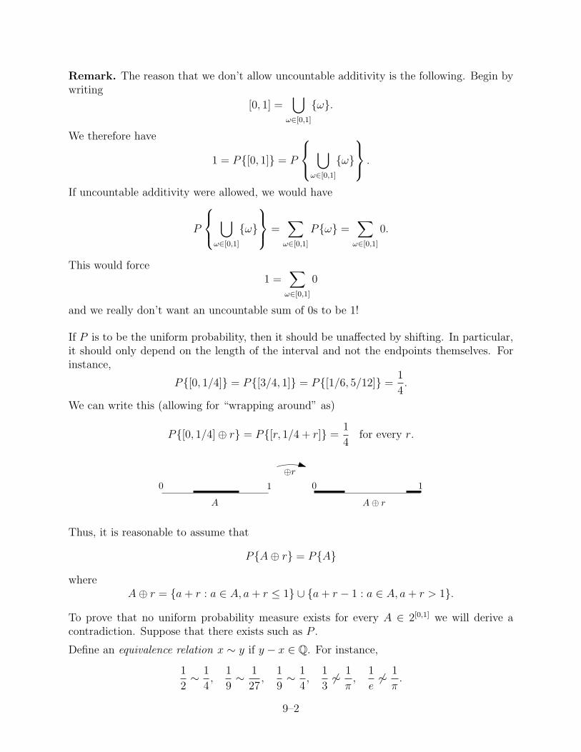
If P is to be the uniform probability, then it should be unaffected by shifting. In particular,it should only depend on the length of the interval and not the endpoints themselves. Forinstance,
P[0, 1/4] = P[3/4, 1] = P[1/6, 5/12] =1
4.
We can write this (allowing for “wrapping around” as)
P[0, 1/4]⊕ r = P[r, 1/4 + r] =1
4for every r.
A A⊕ r
0 1 0 1⊕r
Thus, it is reasonable to assume that
PA⊕ r = PA
whereA⊕ r = a + r : a ∈ A, a + r ≤ 1 ∪ a + r − 1 : a ∈ A, a + r > 1.
To prove that no uniform probability measure exists for every A ∈ 2[0,1] we will derive acontradiction. Suppose that there exists such as P .
Define an equivalence relation x ∼ y if y − x ∈ Q. For instance,
1
2∼ 1
4,
1
9∼ 1
27,
1
9∼ 1
4,
1
36∼ 1
π,
1
e6∼ 1
π.
9–2
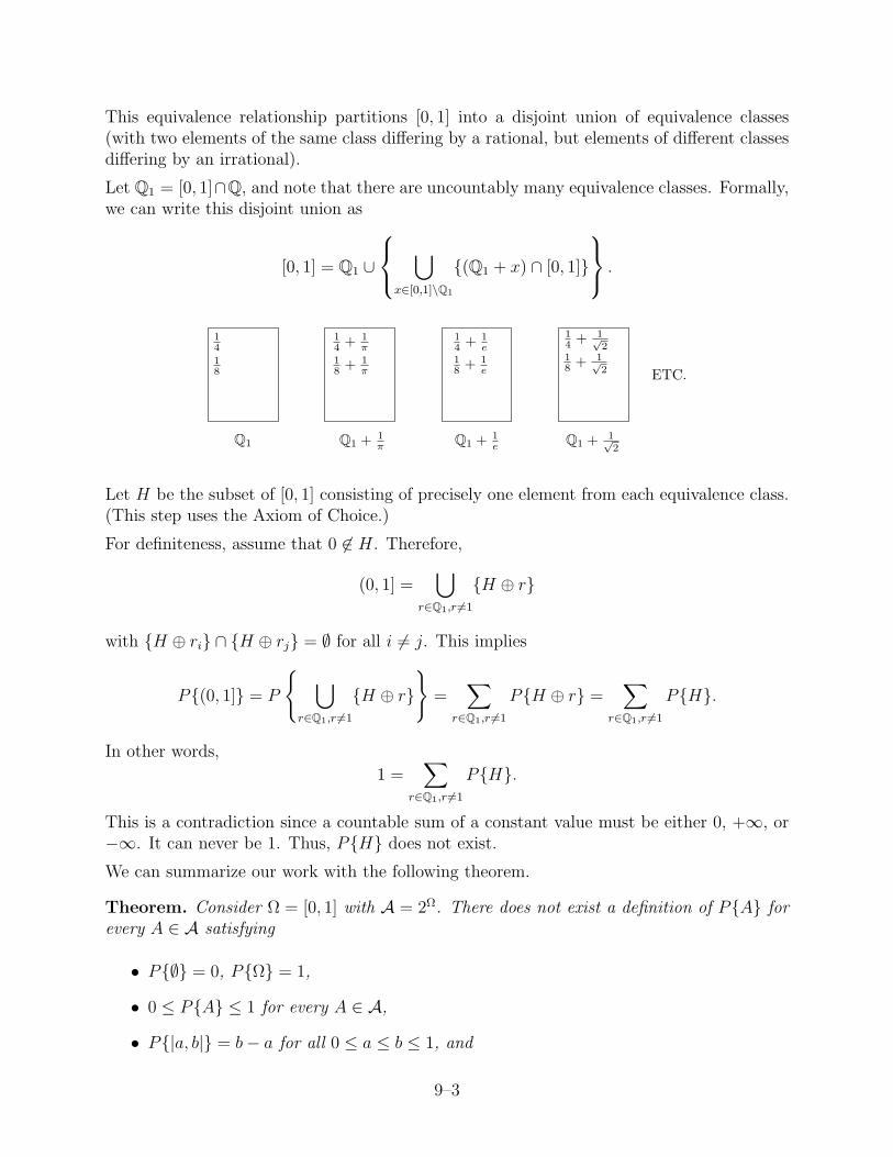
This equivalence relationship partitions [0, 1] into a disjoint union of equivalence classes(with two elements of the same class differing by a rational, but elements of different classesdiffering by an irrational).
Let Q1 = [0, 1]∩Q, and note that there are uncountably many equivalence classes. Formally,we can write this disjoint union as
[0, 1] = Q1 ∪
⋃x∈[0,1]\Q1
(Q1 + x) ∩ [0, 1]
.
Q1 Q1 + 1π Q1 + 1
e Q1 + 1√2
14
14 + 1√
214 + 1
e14 + 1
π
18
18 + 1
π18 + 1
e
18 + 1√
2 ETC.
Let H be the subset of [0, 1] consisting of precisely one element from each equivalence class.(This step uses the Axiom of Choice.)
For definiteness, assume that 0 6∈ H. Therefore,
(0, 1] =⋃
r∈Q1,r 6=1
H ⊕ r
with H ⊕ ri ∩ H ⊕ rj = ∅ for all i 6= j. This implies
P(0, 1] = P
⋃r∈Q1,r 6=1
H ⊕ r
=
∑r∈Q1,r 6=1
PH ⊕ r =∑
r∈Q1,r 6=1
PH.
In other words,
1 =∑
r∈Q1,r 6=1
PH.
This is a contradiction since a countable sum of a constant value must be either 0, +∞, or−∞. It can never be 1. Thus, PH does not exist.
We can summarize our work with the following theorem.
Theorem. Consider Ω = [0, 1] with A = 2Ω. There does not exist a definition of PA forevery A ∈ A satisfying
• P∅ = 0, PΩ = 1,
• 0 ≤ PA ≤ 1 for every A ∈ A,
• P|a, b| = b− a for all 0 ≤ a ≤ b ≤ 1, and
9–3

• if A1, A2, . . . ∈ A are pairwise disjoint, then
P
∞⋃i=1
Ai
=
∞∑i=1
PAi.
Remark. The fact that there exists a A ∈ 2[0,1] such that PA does not exist means thatthe σ-algebra 2[0,1] is simply too big! Instead, the “correct” σ-algebra to use is B1, the Borelsets of [0, 1]. Later we will construct the uniform probability space ([0, 1],B1, P ).
9–4

Statistics 851 (Winter 2008) January 28, 2008Prof. Michael Kozdron
Lecture #10: Construction of a Probability Measure
Reference. Chapter 6 pages 35–38
Suppose that Ω is a sample space. It Ω is finite or countable, then we can construct theprobability space (Ω, 2Ω, P ) without much trouble. However, it is not so easy if Ω is un-countable.
Problem. A “typical” probability on Ω will have
Pω = pω = 0
for all ω ∈ Ω. Hence, pω will NOT characterize P .
Problem. If Ω is uncountable, then, even though 2Ω is a σ-algebra, it will often be toolarge. Thus, we will not be able to define PA for every A ∈ 2Ω.
Solution. Our solution to both these problems is the following. We will consider an algebraA0 with σ(A0) = A.
We will define a function P : A0 → [0, 1] (although P will not necessarily be a probability)and extend P : A → [0, 1] in a unique way (so that P is now a probability).
Remark. When Ω = R, then the structure of R can simplify some things. We will seeexamples of this in Chaper 7.
Definition. A class C of subsets of Ω is closed under finite intersections if for every n < ∞and for every A1, . . . , An ∈ C,
n⋂i=1
Ai ∈ C.
Example. If Ω = a, b, c, d and
C = ∅, a, b, c, a, b, a, c, b, c, a, b, c ,
then C is not a σ-algebra (or even an algebra), but it is closed under finite intersections.
Definition. A class C of subsets of Ω is closed under increasing limits if for every collectionA1, A2, . . . ∈ C with A1 ⊂ A2 ⊂ · · · , then
∞⋃i=1
Ai ∈ C.
A1A2A3∞⋃
i=1
Ai
10–1
Definition. A class C of subsets of Ω is closed under finite differences if for every A, B ∈ Cwith A ⊂ B, then B \ A ∈ C.
A
B
Theorem (Monotone Class Theorem). Let C be a class of subsets of Ω. Suppose that Ccontains Ω (that is, Ω ∈ C) and is closed under finite intersections. Let D be the smallestclass containing C which is closed under increasing limits and finite differences. Then,
D = σ(C).
Example. As in the previous example, suppose that Ω = a, b, c, d and let
C = ∅, a, b, c, a, b, a, c, b, c, a, b, c
so that C is closed under finite intersections. Furthermore, C is also closed under increasinglimits and finite differences as a simple calculation shows. Therefore, ifD denotes the smallestclass containing C which is closed under increasing limits and finite differences, then clearlyD = C itself. However, C is not a σ-algebra; the conclusion of the Monotone Class Theoremsuggests that D = σ(C) which would force C to be a σ-algebra. This is not a contradictionsince the hypothesis that Ω ∈ C is not met. Suppose that
C ′ = C ∪ Ω.
Then C ′ is still closed under finite intersections. However, it is no longer closed under finitedifferences. As a calculation shows, the smallest σ-algebra containing C ′ is now σ(C ′) = 2Ω.
Proof. We begin by noting that the intersection of classes of sets closed under increasinglimits and finite differences is again a class of that type. Hence, if we take the intersectionof all such classes, then there will be a smallest class containing C which is closed underincreasing limits and by finite differences. Denote this class by D. Also note that a σ-algebrais necessarily closed under increasing limits and by finite differences. Thus, we conclude thatD ⊆ σ(C). To complete the proof we will show the reverse containment, namely σ(C) ⊆ D.
For every set B ⊆ Ω, let
DB = A ⊆ Ω : A ∈ D and A ∩B ∈ D.
Since D is closed under increasing limits and finite differences, a calculation shows that DB
must also closed under increasing limits and finite differences.
Since C is closed under finite intersections, C ⊆ DB for every B ∈ C. That is, suppose thatB ∈ C is fixed and let C ∈ C be arbitrary. Since C is closed under finite intersections, wemust have B ∩ C ∈ C. Since C ⊆ D, we conclude that B ∩ C ∈ D verifying that C ∈ DB
10–2
for every B ∈ C. Note that by definition we have DB ⊆ D for every B ∈ C and so we haveshown
C ⊆ DB ⊆ D
for every B ∈ C. Since DB is closed under increasing limits and finite differences, we concludethat D, the smallest class containing C closed under increasing limits and finite differences,must be contained in DB for every B ∈ C. That is, D ⊆ DB for every B ∈ C. Taken together,we are forced to conclude that D = DB for every B ∈ C.
Now suppose that A ∈ D is arbitrary. We will show that C ⊆ DA. If B ∈ C is arbitrary,then the previous paragraph implies that D = DB. Thus, we conclude that A ∈ DB whichimplies that A ∩ B ∈ D. It now follows that B ∈ DA. This shows that C ⊆ DA for everyA ∈ D as required. Since DA ⊆ D for every A ∈ D by definition, we have shown
C ⊆ DA ⊆ D
for every A ∈ D. The fact that D is the smallest class containing C which is closed underincreasing limits and finite differences forces us, using the same argument as above, toconclude that D = DA for every A ∈ D.
Since D = DA for all A ∈ D, we conclude that D is closed under finite intersections.Furthermore, Ω ∈ D and D is closed by finite differences which implies that D is closedunder complementation. Since D is also closed by increasing limits, we conclude that D isa σ-algebra, and it is clearly the smallest σ-algebra containing C. Thus, σ(C) ⊆ D and theproof that D = σ(C) is complete.
Corollary. Let A be a σ-algebra, and let P , Q be two probabilities on (Ω,A). Suppose thatP , Q agree on a class C ⊆ A which is closed under finite intersections. If σ(C) = A, thenP = Q.
Proof. Since A is a σ-algebra we know that Ω ∈ A. Since PΩ = QΩ = 1 we can assumewithout loss of generality that Ω ⊆ C. Define
D = A ∈ A : PA = QA
to be the class on which P and Q agree (and note that ∅ ∈ D and Ω ∈ D so that D isnon-empty). By the definition of probability and Theorem 2.3, we see that D is closed bydifferences and increasing limits. By assumption, we also have C ⊆ D. Therefore, sinceσ(C) = A, we have D = A by the Monotone Class Theorem.
10–3

Statistics 851 (Winter 2008) January 30, 2008Prof. Michael Kozdron
Lecture #11: Null Sets
Reference. Chapter 6 pages 35–38
Definition. Let P be a probability on A. A null set (or a negligible set) for P is a subsetA ⊆ Ω such that there exists a B ∈ A with A ⊆ B and PB = 0.
Note. Suppose that B ∈ A with PB = 0. Let A ⊆ B as shown below.
A
B
If A ∈ A, then we can conclude that PA = 0. However, if A 6∈ A, then PA does notmake sense.
In either case, A is a null set. Thus, it is natural to define PA = 0 for all null sets.
Theorem. Suppose that (Ω,A, P ) is a probability space so that P is a probability on theσ-algebra A. Let N denote the set of all null sets for P . Let
A′ = A ∪N = A ∪N : A ∈ A, N ∈ N.
Then A′ is a σ-algebra, called the P -completion of A, and is the smallest σ-algebra containingA and N . Furthermore, P extends uniquely to a probability on A′ (also called P ) by setting
PA ∪N = PA
for A ∈ A, N ∈ N .
Notation. We say that “Property B” holds almost surely if
Pω : Property B does not hold = 0,
i.e., if ω : Property B does not hold is a null set.
Construction of Probabilities on R
Reference. Chapter 7 pages 39–44
Recall that by a probability space (Ω,A, P ) we mean a triple where Ω is the sample space,A is a σ-algebra of subsets of Ω, and P : A → [0, 1] is a probability measure.
11–1
A random variable is a special kind of function from Ω to R. Schematically, we write
X : Ω → Rω 7→ X(ω)
If Ω is finite or countable, then ANY function X : Ω → R is a random variable.
However, if Ω is uncountable, then there are functions which are NOT random variables.
Example. Suppose that Ω = [0, 1] and H ⊂ Ω is the non-measurable set constructed inLecture #9. The function X : Ω → R defined by
X(ω) = 1Hω
is not a random variable. (This fact will be proved later.)
Also recall that if Ω is finite or countable, then we take A = 2Ω as our σ-algebra.
However, if Ω is uncountable, then the σ-algebra 2Ω is too big. Thus, we must use a σ-algebraB ( 2Ω.
If Ω ⊆ R and is uncountable, say Ω = [0, 1] or Ω = R, then the “correct” σ-algebra to use isthe Borel σ-algebra B. To emphasize the Borel sets of Ω we write B(Ω).
Recall that the Borel σ-algebra is generated by the open sets so that B = σ(O). For instance,B([0, 1]) = σ(O) where O denotes the set of open subsets of [0, 1].
Fact. By Theorem 2.1, we know that B is generated by intervals of the form (−∞, a] fora ∈ Q.
Suppose that X : Ω → R is a random variable. (This is not yet defined.) We have alreadyseen that X induces a probability measure on (R,B) denoted by PX where
PXB = Pω : X(ω) ∈ B = PX ∈ B = PX−1(B) for every B ∈ B
is called the law of X. Hence, we see that X transforms the probability space (Ω,A, P ) intothe probability space (R,B, PX):
X : (Ω,A, P ) → (R,B, PX).
Since the law of a random variable is always a probability measure on (R,B) (not yet proved)we have good reason to study probabilities on R. This motivates Chapter 7.
Definition. Suppose that P is a probability measure on (R,B). The distribution functioninduced by P is the function F : R → [0, 1] defined by
F (x) = P(−∞, x] for all x ∈ R.
Note. Since
(−∞, x] =∞⋂
n=1
(−∞, x + 1
n
)is the countable intersection of open sets, we see that (−∞, x] ∈ B for every x ∈ R. Thus,P(−∞, x] makes sense.
11–2

Question. We see that each different probability P gives rise to a distribution function F(i.e., P F ). Is the converse true? That is, does P uniquely characterize F and vice-versa?
The answer is yes—knowledge of F uniquely determines P as the following theorem shows.
Theorem. The distribution function F induced by P characterizes P .
Proof. (Sketch) Suppose that we know F (x) for every x ∈ R. We then know
P(−∞, x]
for every x ∈ R. In particular, we know
P(−∞, a]
for every a ∈ Q. Since(−∞, a] : a ∈ Q
generates B(R), we know PB for every B ∈ B.
Question. Can we tell which functions F : R → [0, 1] are distribution functions?
Theorem. A function F : R → [0, 1] is the distribution function of a unique probabilitymeasure P on (R,B) if and only if
(i) F is non-decreasing, i.e., x < y implies F (x) ≤ F (y),
(ii) F is right-continuous, i.e., F (y) → F (x) as y → x+,
limy→x+
F (y) = limy↓x
F (y) = F (x),
(iii) F (x) → 1 as x →∞, i.e.,lim
x→∞F (x) = 1,
(iv) F (x) → 0 as x → −∞, i.e.,lim
x→−∞F (x) = 0.
Example. Suppose that α ∈ R and let
F (x) =
1, if x ≥ α,
0, if x < α.
Since F satisfies all the conditions of the theorem, F must be a distribution function. Thecorresponding probability measure is
PB =
1, if α ∈ B,
0, if α 6∈ B,
for every B ∈ B. We call P the Dirac point mass at α.
11–3

Statistics 851 (Winter 2008) February 1, 2008Prof. Michael Kozdron
Lecture #12: Random Variables
Reference. Chapter 8 pages 47–50
Suppose that (Ω,A, P ) is a probability space and let X : Ω → R given by ω 7→ X(ω) be afunction.
Definition. We say that the function X : Ω → R is a random variable (or a measurablefunction) if X−1(B) ∈ A for every B ∈ B where B denotes the Borel sets of R.
Remark. We use the phrases random variable and measurable function synonymously.“Random variable” is preferred by probabilists while “measurable function” is preferredby analysts.
Note. The motivation for the definition of random variable is the following. We want to beable to compute
Pω : X(ω) ∈ B = PX ∈ B = PX−1(B)
for every B ∈ B. Therefore, we must have X−1(B) ∈ A in order for PX−1(B) to makesense.
Remark. If Ω is either finite or countable, then every function X : (Ω, 2Ω) → (R,B) ismeasurable. If Ω is uncountable, then the trouble begins!
Example. Suppose that (Ω,A, P ) is a probability space and let H 6∈ A so that H is not anevent. We saw an example of such a non-measurable H in Lecture #9. Define the functionX : Ω → R by setting
X(ω) = 1Hω =
1, if ω ∈ H,
0, if ω 6∈ H.
To prove that the function X is not a random variable, we must show that there exists aBorel set B ∈ B for which X−1(B) 6∈ A. Let B = 1 which is clearly a closed set andtherefore Borel. We find
X−1(1) = ω : X(ω) = 1 = ω : ω ∈ H = H.
However, by assumption, H 6∈ A so that X−1(1) 6∈ A. Thus, X is not a random variable.
Remark. Note that in order for the previous example to work we must have A ( 2Ω. Inthe case of a discrete or countable Ω our standard choice of A = 2Ω makes such an exampleimpossible. It is, however, possible to construct a probability space on a discrete space Ω insuch a way that A 6= 2Ω. For instance, let Ω = a, b, c, d and take A = ∅, a, b, c, d, Ω.Set Pa, b = Pc, d = 1/2. If H = a, then H is not an event and X(ω) = 1Hω is nota random variable. However, this example is both silly and contrived!
12–1

Definition. If X : Ω → R is a random variable, then the law (or distribution) of X is theprobability measure on (R,B) given by
PXB = Pω : X(ω) ∈ B = PX ∈ B = PX−1(B)
for every B ∈ B.
Although we have referred to the fact that PX is a probability on (R,B), we have not yetproved it!
Theorem. The law of a random variable X : (Ω,A, P ) → (R,B) is a probability measureon (R,B).
Proof. In order to prove this result, we must verify the conditions of Definition 2.3 are met.We begin by noting that B is, by definition, a σ-algebra on R. Since ∅ ∈ B, we have
PX∅ = Pω : X(ω) ∈ ∅ = P∅ = 0
using the fact that ∅ ∈ A and P is a probability on (Ω,A). Suppose that B1, B2, . . . ∈ B isa sequence of pairwise, disjoint sets. Therefore,
PX
∞⋃i=1
Bi
= P
ω : X(ω) ∈
∞⋃i=1
Bi
= P
ω : ω ∈
∞⋃i=1
X−1(Bi)
= P
ω : ω ∈
∞⋃i=1
Ai
where Ai = X−1(Bi). Since X is a random variable, we know that Ai ∈ A for each i =1, 2, . . .. Moreover, A1, A2, . . . are pairwise disjoint. Thus, using the fact that A1, A2, . . . ∈ Aare pairwise disjoint and P is a probability on (Ω,A) gives
PX
∞⋃i=1
Bi
= P
∞⋃i=1
Ai
=
∞∑i=1
PAi =∞∑i=1
PX−1(Bi) =∞∑i=1
PXBi
as required.
Since PX is a probability measure on (R,B) we can discuss the corresponding distributionfunction.
Definition. If X : Ω → R is a random variable, then the distribution function of X, writtenFX : R → [0, 1], is defined by
FX(x) = PX(−∞, x] = Pω : X(ω) ≤ x = PX ≤ x
for every x ∈ R.
Remark. By Theorem 7.1, distribution functions characterize probabilities on R. That is,knowledge of one gives knowledge of the other:
X (random variable)! PX (law of X)! FX (distribution function of X)
Remark. In Jacod and Protter, things are proved in a bit more generality. A functionX : (E, E) → (F,F) is called measurable if X−1(B) ∈ E for every B ∈ F . A space E anda σ-algebra E of subsets of E together are often called a measurable space. Technically, it isonly when we introduce probability measures onto (E, E) do measurable functions becomerandom variables.
12–2

Summary of Important Objects
At this point, we have introduced all of the objects that are most important to modernprobability. It is worth memorizing each of the definitions.
• Ω, the sample space of outcomes ω ∈ Ω,
• A, a σ-algebra of subsets of Ω (Definition 2.1),
• P , a set function from A to [0, 1] (Definition 2.3),
• (Ω,A) is called a measurable space and (Ω,A, P ) is called a probability space,
• the real numbers R together with the Borel sets B is a measurable space (Theorem 2.1),
• X : Ω → R is a random variable (Definition 8.1),
• PX is the law of X (page 50),
• FX is the distribution function of X (Definition 7.1),
• (R,B, PX) is a probability space (Theorem 8.5).
It is important to know when a function of a random variable is again a random variable.The following theorem gives the answer.
Theorem. Let X : Ω → R be a random variable and let f : R → R be measurable. If thefunction f X : Ω → R is defined by
f X(ω) = f(X(ω)),
then f X is a random variable.
Proof. To show that f X is a random variable, we must show that
(f X)−1(B) ∈ A
for every B ∈ B. Since f : R → R is measurable, we know that
f−1(B) ∈ B
for every B ∈ B. Since X : (Ω,A) → (R,B) is a random variable, we know that
X−1(B) ∈ A
for every B ∈ B. Since f−1(B) ∈ B, it must be the case that X−1(f−1(B)) ∈ A. Since
(f X)−1(B) = X−1(f−1(B))
the proof is complete.
12–3
The next theorem extends the example we considered at the beginning of this lecture.
Theorem. Suppose that (Ω,A, P ) is a probability space and A ⊆ Ω. The function 1A : Ω →R given by
1Aω =
1, if ω ∈ A,
0, if ω 6∈ A,
is a random variable if and only if A ∈ A.
Proof. For B ⊆ R, we find
(1A)−1(B) =
∅, if 0 6∈ B, 1 6∈ B,
A, if 0 6∈ B, 1 ∈ B,
Ac, if 0 ∈ B, 1 6∈ B,
Ω, if 0 ∈ B, 1 ∈ B.
Thus, (1A)−1(B) ∈ A if and only if B ∈ B.
12–4
Statistics 851 (Winter 2008) February 4, 2008Prof. Michael Kozdron
Lecture #13: Random Variables
Reference. Chapter 8 pages 47–50
Theorem. Suppose that X : Ω → R is a function. X is a random variable if and only ifX−1(O) ∈ A for every open set O ∈ O.
Proof. We being by recalling that the Borel sets are the σ-algebra generated by the opensets. That is, B = σ(O) where O = open sets. If X is a random variable, then since anopen set is necessarily a Borel set we have the forward implication X−1(O) ∈ A for everyopen set O ∈ O. To show that converse, suppose that X−1(O) ∈ A for every open setO ∈ O. We must now show that X−1(B) ∈ A for every Borel set B ∈ B. We leave it as anexercise to verify that that the following set relations hold:
X−1
(⋃n
Bn
)=⋃n
X−1(Bn), X−1
(⋂n
Bn
)=⋂n
X−1(Bn), and X−1(Bc) =[X−1(B)
]c.
Our strategy for the proof is the following. Let F = B ∈ B : X−1(B) ∈ A. We willshow that F = B. On the one hand, F ⊆ B by definition. On the other hand, since X−1
commutes with unions, intersections, and complements, we see that F is a σ-algebra. Byassumption O ⊆ F which implies that σ(O) ⊆ F since F is a σ-algebra. Since σ(O) = Bwe conclude B ⊆ F . Thus, we have shown
B ⊆ F ⊆ B
which implies that B = F . In other words,
X−1(B) ⊆ σ(X−1(O)) ⊆ A
meaning that X−1(B) ∈ A for every B ∈ B.
Theorem. Suppose that X : Ω → R and Xn : Ω → R, n = 1, 2, . . . are functions.
(a) X is a random variable if and only if X ≤ a = X−1((−∞, a]) ∈ A for every a ∈ Rif and only if X < a ∈ A for every a ∈ R.
(b) If Xn, n = 1, 2, . . ., are each random variables, then
supn
Xn, infn
Xn, lim supn→∞
Xn, lim infn→∞
Xn
are also random variables.
(c) If Xn, n = 1, 2, . . ., are each random variables and Xn → X pointwise, then X is arandom variable.
13–1
Proof. (a) By Theorem 2.1, we know that
σ((−∞, a] : a ∈ R) = B
and so the result follows from the previous theorem. Recall that we write
(−∞, a) =∞⋃
n=1
(−∞, a− 1
n
].
(b) Since Xn is a random variable, we see that Xn ≤ a = Xn(ω) ∈ (−∞, a] ∈ A foreach n. By definition,
supn
Xn ≤ a
=⋂n
Xn ≤ a ∈ A
and infn
Xn < a
=⋃n
Xn < a ∈ A
so that both of these are random variables by (a). Since
lim supn→∞
Xn = infn
supm≥n
Xm,
if we defineYn = sup
m≥nXm,
then Yn is a random variable so thatinfn
Yn
is also a random variable. The proof that
lim infn→∞
Xn = supn
infm≥n
Xm
is a random variable is similar.
(c) If Xn → X pointwise, then
X = limn→∞
Xn = lim infn→∞
Xn = lim supn→∞
Xn
is a random variable by (b).
13–2
Density Functions
Reference. Chapter 7 pages 42–44
Suppose that f : R → [0,∞) is non-negative and Riemann-integrable with∫ ∞
−∞f(x) dx = 1.
Define the function F : R → [0, 1] by setting
F (x) =
∫ x
−∞f(y) dy.
It then follows that F is non-decreasing, F is right-continuous, F (x) → 1 as x → ∞, andF (x) → 0 as x → −∞. In other words, F is a distribution function. (Check these facts!)We call f the density (function) associated to F .
Remark. It is not true that every distribution admits a density. For instance, there is nodensity associated with the Dirac point mass at α. However, many “famous” distributionsadmit densities.
Example. The uniform distribution on (a, b) has density
f(x) =
1
b−a, if a < x < b,
0, otherwise.
Example. The exponential distribution with parameter β > 0 has density
f(x) =
βe−βx, if x > 0,
0, otherwise.
Example. The normal distribution with parameters σ > 0, µ ∈ R, has density
f(x) =1
σ√
2πexp
−(x− µ)2
2σ2
, x ∈ R.
Note. See pages 43–44 for other examples of densities.
Remark. Suppose X : Ω → R is a random variable. As we have already seen, PX , the lawof X, is a probability measure on (R,B). Hence, we say that X has density function fX iffX is the density associated with FX , the distribution function of X.
Example. Consider the probability space (Ω,A, P ) where Ω = [0, 1], A = B([0, 1]), and Pis the uniform probability on [0, 1]. Let X : Ω → R be defined by
X(ω) =
1, if ω ∈ Q ∩ [0, 1],
0, otherwise.
13–3
Note that X is the indicator function of the rational numbers in [0, 1]. As we have alreadyseen, X is a random variable if and only if Q ∩ [0.1] ∈ A. Is it? We write Q1 = Q ∩ [0, 1] sothat
Q1 =⋂
ω∈Q1
ω
expresses Q1 as a countable union of disjoint closed sets. Thus, Q1 is a Borel set so thatQ1 ∈ A is measurable and X = 1Q1 is a random variable. Let the function Y : Ω → R bedefined by Y (ω) = ωX(ω). Is Y a random variable?
Here are some other questions to keep us thinking.
• What “type” of random variable is X? What about Y ?
• What is PX? What is P Y ?
• Does PX have a distribution function FX? What about P Y ?
• Do either FX or FY admit a density?
• What is E(X), E(X2), E(Y ), or E(Y 2)?
13–4

Statistics 851 (Winter 2008) February 6, 2008Prof. Michael Kozdron
Lecture #14: Some General Function Theory
Suppose that f : X → Y is a function. We are implicitly assuming that f is defined for allx ∈ X. We call X the domain of f and call Y the codomain of f .
The range of f is the set
f(X) = y ∈ Y : f(x) = y for some x ∈ X.
Note that f(X) ⊆ Y. If f(X) = Y, then we say that f is onto Y.
Let B ⊆ Y. We define f−1(B) by
f−1(B) = x ∈ X : f(x) = y for some y ∈ B = f ∈ B = x : f(x) ∈ B.
We call X a topological space if there is a notion of open subsets of X. The Borel σ-algebraon X, written B(X), is the σ-algebra generated by the open sets of X.
Let X and Y be topological spaces. A function f : X → Y is called continuous if for everyopen set V ⊆ Y, the set U = f−1(V ) ⊆ X is open.
A function f : X → Y is called measurable if for every measurable set B ∈ B(Y), the setf−1(B) ∈ B(X) is a measurable set.
The proof of the first theorem proved in Lecture #13 can be generalized without any difficultyto yield the following result.
Theorem. Suppose that (X,B(X)) and (Y,B(Y)) are topological measure spaces. The func-tion f : X → Y is measurable if and only if f−1(O) ∈ B(X) for every open set O ∈ B(Y).
The next theorem tells us that continuous functions are necessarily measurable functions.
Theorem. Suppose that (X,B(X)) and (Y,B(Y)) are topological measure spaces. If f :X → Y is continuous, then f is measurable.
Proof. By definition, f : X → Y is continuous if and only if f−1(O) ⊆ X is an open setfor every open set O ⊆ Y. Since an open set is necessarily a Borel set, we conclude thatf−1(O) ∈ B(X) for every open set O ∈ B(Y). However, it now follows immediately fromthe previous theorem that f : X → Y is measurable.
The following theorem is a generalization of a theorem proved in Lecture #12 and showsthat the composition of measurable functions is measurable.
Theorem. Suppose that (W,F), (X,G), and (Y,H) are measurable spaces, and let f :(W,F) → (X,G) and g : (X,G) → (Y,H) be measurable. Then the function h = g f is ameasurable function from (W,F) to (Y,H).
14–1
Proof. Suppose that H ∈ H. Since g is measurable, we have g−1(H) ∈ G. Since f ismeasurable, we have f−1(g−1(H)) ∈ F . Since
h−1(H) = (g f)−1(H) = f−1(g−1(H)) ∈ F
the proof is complete.
Recall that from Theorem 2.1 the Borel sets of R are generated by intervals of the form(−∞, a] for a ∈ Q. Exactly the same proof shows that the Borel sets of Rn, written Bn =B(Rn) are generated by quadrants of the form
n∏i=1
(−∞, ai], a1, . . . , an ∈ Q.
Theorem. Let (Ω,A, P ) be a probability space and suppose that Xi : Ω → R is a randomvariable for each i = 1, . . . , n. Suppose further that f : (Rn,Bn) → (R,B) is measurable.Then the function f(X1, . . . , Xn) : Ω → R is measurable.
Proof. Define the (vector-valued) function X : Ω → Rn by setting X(ω) = (X1(ω), . . . , Xn(ω)).Since
X−1
(n∏
i=1
(−∞, ai]
)=
n⋂i=1
X−1i ((−∞, ai]) =
n⋂i=1
Xi ≤ ai ∈ A
we conclude that X : Ω → Rn is measurable. We often call X a random vector. SinceX : Ω → Rn is measurable and f : Rn → R is measurable, we immediately conclude fromthe previous theorem f X = f(X1, . . . , Xn) : Ω → R is measurable.
Corollary. If X and Y are random variables, then so too are X +Y , XY , X/Y for Y 6= 0,X ∧ Y , and X ∨ Y .
Expectation
Reference. Chapter 9 pages 51–60
Suppose that (Ω,A, P ) is a probability space and let X : (Ω,A) → (R,B) be a randomvariable. Recall that this means that X−1(B) ∈ A for every B ∈ B. Our goal in this lectureis the following.
Goal. To define E(X) for every random variable X.
Definition. A random variable X : Ω → R is called simple if it can be written as
X =n∑
i=1
ai1Ai
where ai ∈ R, Ai ∈ A for i = 1, 2, . . . , n.
14–2
Note that if a random variable is simple, then it takes on a finite number of values. As thenext proposition shows, the converse is also true.
Proposition. If X : Ω → R is a random variable that takes on finitely many values, thenX is simple.
Proof. Suppose X is a random variable and takes on finitely many values labelled a1, . . . , an.Let
Ai = X = ai = ω : X(ω) = ai, i = 1, . . . , n.
Since X is a random variable, Ai = X−1(ai), and ai is a Borel set, we conclude thatAi ∈ A for each i = 1, . . . , n. Furthermore, we can represent X as
X =n∑
i=1
ai1Ai
which proves that X is simple.
Thus, saying that X is a simple random variable means that the range of X is finite.
Remark. Recall that the function X = 1A is measurable if and only if A ∈ A. Also recallthat the composition and sum of measurable functions is again measurable. Therefore, wesee that
X =n∑
i=1
ai1Ai
is measurable if and only if Ai ∈ A for each i = 1, . . . , n.
Definition. If X is a simple random variable, then the expectation (or expected value) of Xis defined to be
E(X) =n∑
i=1
aiPAi.
Remark. By definition, a simple random variable is necessarily discrete. However, theconverse is not true. For instance, if Y is a Poisson(λ) random variable, then
PY = k > 0 for every k = 0, 1, 2, . . .
so that Y is a discrete random variable which is not simple.
Example. Consider the probability space (Ω,A, P ) where Ω = [0, 1], A = B(Ω) are theBorel sets in [0, 1], and P is the uniform probability measure on [0, 1]. Let Q1 = [0, 1] ∩ Qand consider the random variable X = 1Q1 which is given by
X(ω) =
1, if ω ∈ [0, 1] ∩Q,
0, if ω 6∈ [0, 1] ∩Q.
Since the only two possible values of X are 0 and 1, we conclude that X is simple. Therefore,if we let a1 = 1 and a2 = 0 so that A1 = Q1 and A2 = [0, 1] \Q1, then
E(X) = a1PA1+ a2PA2 = PQ1 = 0
since PQ1 = 0.
14–3
A slight extension of this example is given by the following exercise.
Exercise. Suppose that (Ω,A, P ) is the same probability space as in the previous example.Let A ⊂ Ω be countable and define the function X : Ω → R by setting X(ω) = 1A(ω). Provethat A ∈ A with PA = 0 so that X is a random variable with E(X) = 0.
Example. Suppose that (Ω,A, P ) is the same probability space and X is the same randomvariable as in the previous example. Define the function Y : Ω → R by setting Y (ω) = 0 forall ω ∈ Ω. Therefore, Y is a simple random variable with E(Y ) = 0. Notice that both E(X)and E(Y ) equal 0. However, X 6= Y since, for instance, X(1/2) = 1 but Y (1/2) = 0. Theset where X and Y differ is
X 6= Y = ω : X(ω) 6= Y (ω) = ω : X(ω) = 1, Y (ω) = 0 = ω : ω ∈ [0, 1] ∩Q.
However, Pω : ω ∈ [0, 1] ∩Q = 0 so that
PX 6= Y = 0.
In other words, X 6= Y is a null set so that X = Y almost surely. If we now define thefunction Z : Ω → R by setting
Z(ω) =
1, if ω ∈ [0, 1/2],
−1, if ω 6∈ [0, 1/2],
then Z is a simple random variable with E(Z) = 0. However, PZ 6= Y = 1 sinceZ 6= Y = Ω and PZ 6= X = 1 since PZ = X = P[0, 1/2] ∩Q ≤ P[0, 1] ∩Q = 0.Therefore, neither X 6= Z nor Y 6= Z is a null set.
14–4

Statistics 851 (Winter 2008) February 8, 2008Prof. Michael Kozdron
Lecture #15: Expectation of a Simple Random Variable
Reference. Chapter 9 pages 51–60
Recall that a simple random variable is one that takes on finitely many values.
Definition. A random variable X : Ω → R is called simple if it can be written as
X =n∑
i=1
ai1Ai
where ai ∈ R, Ai ∈ A for i = 1, 2, . . . , n.
Example. Consider the probability space (Ω,A, P ) where Ω = [0, 1], A = B(Ω), and P isthe uniform probability on Ω. Suppose that the random variable X : Ω → R is defined by
X(ω) =4∑
i=1
ai1Ai(ω)
where a1 = 4, a2 = 2, a3 = 1, a4 = −1, and
A1 = [0, 12), A2 = [1
4, 3
4), A3 = (1
2, 7
8], A4 = (7
8, 1].
Show that there exist finitely many real constants c1, . . . , cn and disjoint sets C1, . . . , Cn ∈ Asuch that
X =n∑
i=1
ci1Ci.
Solution. We find
X(ω) =
4, if 0 ≤ ω < 1/4,
6, if 1/4 ≤ ω < 1/2,
2, if ω = 1/2,
3, if 1/2 < ω < 3/4,
1, if 3/4 ≤ ω < 7/8,
0, if ω = 7/8,
−1, if 7/8 < ω ≤ 1,
so that
X =7∑
i=1
ci1Ci
where c1 = 4, c2 = 6, c3 = 2, c4 = 3, c5 = 1, c6 = 0, c7 = −1 and
C1 = [0, 14), C2 = [1
4, 1
2), C3 = 1
2, C4 = (1
2, 3
4), C5 = [3
4, 7
8), C6 = 7
8, C7 = (7
8, 1].
15–1
Proposition. If X and Y are simple random variables, then
E(αX + βY ) = αE(X) + βE(Y )
for every α, β ∈ R.
Proof. Suppose that X and Y are simple random variables with
X =n∑
i=1
ai1Aiand Y =
m∑j=1
bj1Bj
where A1, . . . , An ∈ A and B1, . . . , Bm ∈ A each partition Ω. Since
αX = α
n∑i=1
ai1Ai=
n∑i=1
(αai)1Ai
we conclude by definition that
E(αX) =n∑
i=1
(αai)PAi = αn∑
i=1
aiPAi = αE(X).
The proof of the theorem will be completed by showing E(X + Y ) = E(X) + E(Y ). Noticethat
Ai ∩Bj : 1 ≤ i ≤ n, 1 ≤ j ≤ m
consists of pairwise disjoint events whose union is Ω and
X + Y =n∑
i=1
m∑j=1
(ai + bj)1Ai∩Bj.
Therefore, by definition,
E(X + Y ) =n∑
i=1
m∑j=1
(ai + bj)PAi ∩Bj
=n∑
i=1
m∑j=1
aiPAi ∩Bj+n∑
i=1
m∑j=1
bjPAi ∩Bj
=n∑
i=1
aiPAi+m∑
j=1
bjPBj
and the proof is complete.
Fact. If X and Y are simple random variables with X ≤ Y , then
E(X) ≤ E(Y ).
Exercise. Prove the previous fact.
15–2
Goal. To construct E(X) for any random variable.
We have already defined E(X) for simple random variables.
Suppose that X is a positive random variable. That is, X(ω) ≥ 0 for all ω ∈ Ω. (We willneed to allow X(ω) ∈ [0, +∞] for some consistency.)
Definition. If X is a positive random variable, define the expectation of X to be
E(X) = supE(Y ) : Y is simple and 0 ≤ Y ≤ X.
That is, we approximate positive random variables by simple random variables. Of course,this leads to the question of whether or not this is possible.
Fact. For every random variable X ≥ 0, there exists a sequence (Xn) of positive, simplerandom variables with Xn ↑ X (that is, Xn increases to X).
An example of such a sequence is given by
Xn(ω) =
k2n , if k
2n ≤ X(ω) < k+12n and 0 ≤ k ≤ n2n − 1,
n, if X(ω) ≥ n.
(Draw a picture.)
Fact. If X ≥ 0 and (Xn) is a sequence of simple random variables with Xn ↑ X, thenE(Xn) ↑ E(X).
Now suppose that X is any random variable. Write
X+ = maxX, 0 and X− = −minX, 0
for the positive part and the negative part of X, respectively.
Note that X+ ≥ 0 and X− ≥ 0 so that the positive part and negative part of X are bothpositive random variables and
X = X+ −X− and |X| = X+ + X−.
Definition. A random variable X is called integrable (or has finite expectation) if bothE(X+) and E(X−) are finite. In this case we define E(X) to be
E(X) = E(X+)− E(X−).
Definition. If one of E(X+) or E(X−) is infinite, then we can still define E(X) by setting
E(X) =
+∞, if E(X+) = +∞ and E(X−) < ∞,
−∞, if E(X+) < ∞ and E(X−) = +∞.
However, X is not integrable in this case.
Definition. If both E(X+) = +∞ and E(X−) = +∞, then E(X) does not exist.
15–3

Summary of Constructing E(X) for General Random Variables
The outline of how to construct E(X) is sometimes called the “standard machine” and followsthese steps.
(1) Step 1: define E(X) for simple random variables,
(2) Step 2: define E(X) for positive random variables,
(3) Step 3: define E(X) for general random variables.
Of course, we still have to prove that all of the facts given above are true.
15–4

Statistics 851 (Winter 2008) February 11, 2008Prof. Michael Kozdron
Lecture #16: Integration and Expectation
Reference. Chapter 9 pages 51–60
Definition. If X is a positive random variable, then we define
E(X) = supE(Y ) : Y is simple and 0 ≤ Y ≤ X.
If X is any random variable, then we can write X = X+ −X− where both X+ and X− arepositive random variables. Provided that both E(X+) and E(X−) are finite, we define E(X)to be
E(X) = E(X+)− E(X−)
and we say that X is integrable (or has finite expectation).
Remark. If X : (Ω,A, P ) → (R,B, PX) is a random variable, then we sometimes write
E(X) =
∫Ω
X dP =
∫Ω
X(ω) dP (ω) =
∫Ω
X(ω) P (dω).
That is, the expectation of a random variable is the Lebesgue integral of X. We will saymore about this later.
Definition. Let L1(Ω,A, P ) be the set of real-valued random variables on (Ω,A, P ) withfinite expectation. That is,
L1(Ω,A, P ) = X : (Ω,A, P ) → (R,B) : X is a random variable with E(X) < ∞.
We will often write L1 for L1(Ω,A, P ) and suppress the dependence on the underlyingprobability space.
Theorem. Suppose that (Ω,A, P ) is a probability space, and let X1, X2, . . ., X, and Y allbe real-valued random variables on (Ω,A, P ).
(a) L1 is a vector space and expectation is a linear map on L1. Furthermore, expectationis positive. That is, if X, Y ∈ L1 with 0 ≤ X ≤ Y , then 0 ≤ E(X) ≤ E(Y ).
(b) X ∈ L1 if and only if |X| ∈ L1, in which case we have
|E(X)| ≤ E(|X|).
(c) If X = Y almost surely (i.e., if Pω : X(ω) = Y (ω) = 1), then E(X) = E(Y ).
(d) (Monotone Convergence Theorem) If the random variables Xn ≥ 0 for all n and Xn ↑X (i.e., Xn → X and Xn ≤ Xn+1), then
limn→∞
E(Xn) = E(
limn→∞
Xn
)= E(X).
(We allow E(X) = +∞ if necessary.)
16–1

(e) (Fatou’s Lemma) If the random variables Xn all satisfy Xn ≥ Y almost surely for someY ∈ L1 and for all n, then
E(lim infn→∞
Xn
)≤ lim inf
n→∞E(Xn). (∗)
In particular, (∗) holds if Xn ≥ 0 for all n.
(f) (Lebesgue’s Dominated Convergence Theorem) If the random variables Xn → X, andif for some Y ∈ L1 we have |Xn| ≤ Y almost surely for all n, then Xn ∈ L1, X ∈ L1,and
limn→∞
E(Xn) = E(X).
Remark. This theorem contains ALL of the central results of Lebesgue integration theory.
Theorem. Let Xn be a sequence of random variables.
(a) If Xn ≥ 0 for all n, then
E
(∞∑
n=1
Xn
)=
∞∑n=1
E(Xn) (∗)
with both sides simultaneously being either finite or infinite.
(b) If∞∑
n=1
E(Xn) < ∞,
then∞∑
n=1
Xn
converges almost surely to some random variable Y ∈ L1. In other words,
∞∑n=1
Xn
is integrable with
E
(∞∑
n=1
Xn
)=
∞∑n=1
E(Xn).
Thus, (∗) holds with both sides being finite.
Notation. Since X = Y almost surely implies E(X) = E(Y ), we can consider “almost sureequality” as an equivalence relation; that is,
X ∼ Y if X = Y almost surely.
Let L1 denote L1 modulo almost sure equality.
16–2
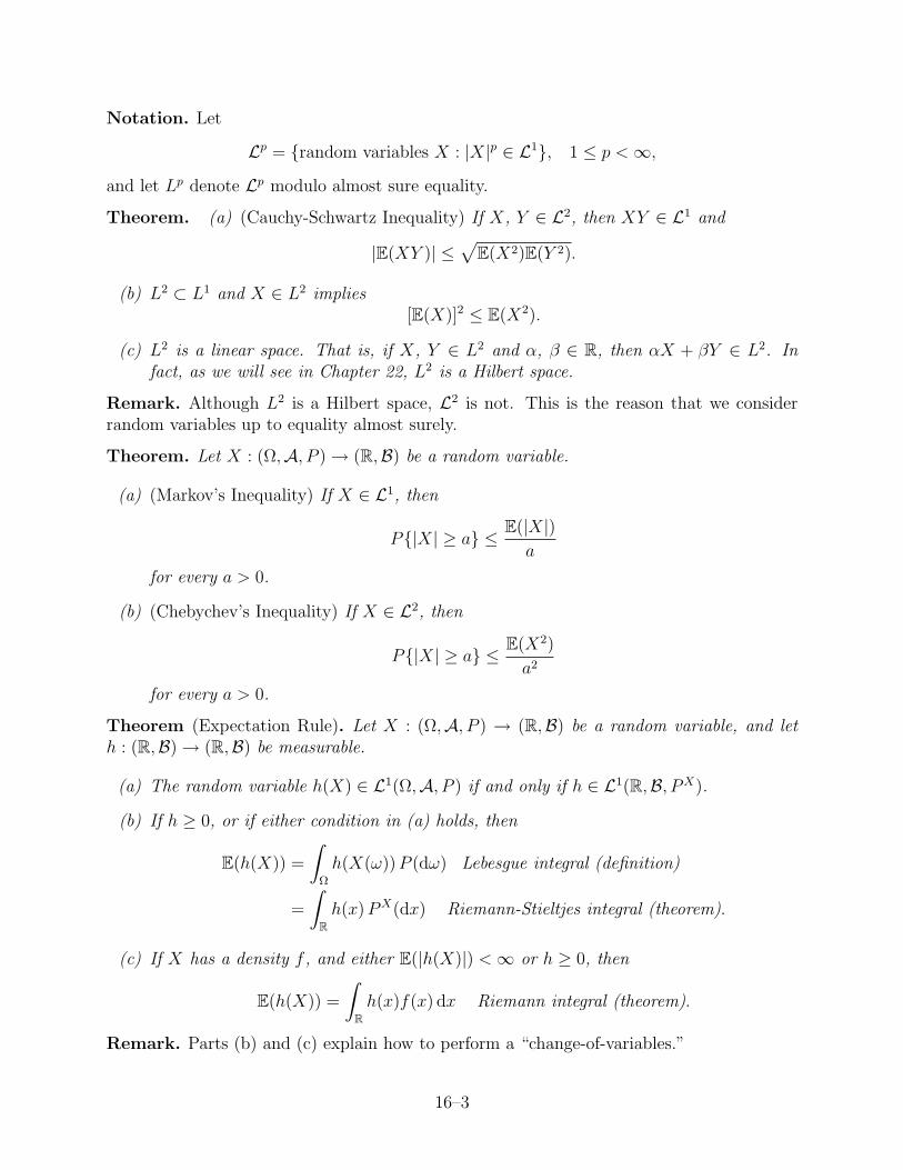
Notation. Let
Lp = random variables X : |X|p ∈ L1, 1 ≤ p < ∞,
and let Lp denote Lp modulo almost sure equality.
Theorem. (a) (Cauchy-Schwartz Inequality) If X, Y ∈ L2, then XY ∈ L1 and
|E(XY )| ≤√
E(X2)E(Y 2).
(b) L2 ⊂ L1 and X ∈ L2 implies[E(X)]2 ≤ E(X2).
(c) L2 is a linear space. That is, if X, Y ∈ L2 and α, β ∈ R, then αX + βY ∈ L2. Infact, as we will see in Chapter 22, L2 is a Hilbert space.
Remark. Although L2 is a Hilbert space, L2 is not. This is the reason that we considerrandom variables up to equality almost surely.
Theorem. Let X : (Ω,A, P ) → (R,B) be a random variable.
(a) (Markov’s Inequality) If X ∈ L1, then
P|X| ≥ a ≤ E(|X|)a
for every a > 0.
(b) (Chebychev’s Inequality) If X ∈ L2, then
P|X| ≥ a ≤ E(X2)
a2
for every a > 0.
Theorem (Expectation Rule). Let X : (Ω,A, P ) → (R,B) be a random variable, and leth : (R,B) → (R,B) be measurable.
(a) The random variable h(X) ∈ L1(Ω,A, P ) if and only if h ∈ L1(R,B, PX).
(b) If h ≥ 0, or if either condition in (a) holds, then
E(h(X)) =
∫Ω
h(X(ω)) P (dω) Lebesgue integral (definition)
=
∫R
h(x) PX(dx) Riemann-Stieltjes integral (theorem).
(c) If X has a density f , and either E(|h(X)|) < ∞ or h ≥ 0, then
E(h(X)) =
∫R
h(x)f(x) dx Riemann integral (theorem).
Remark. Parts (b) and (c) explain how to perform a “change-of-variables.”
16–3
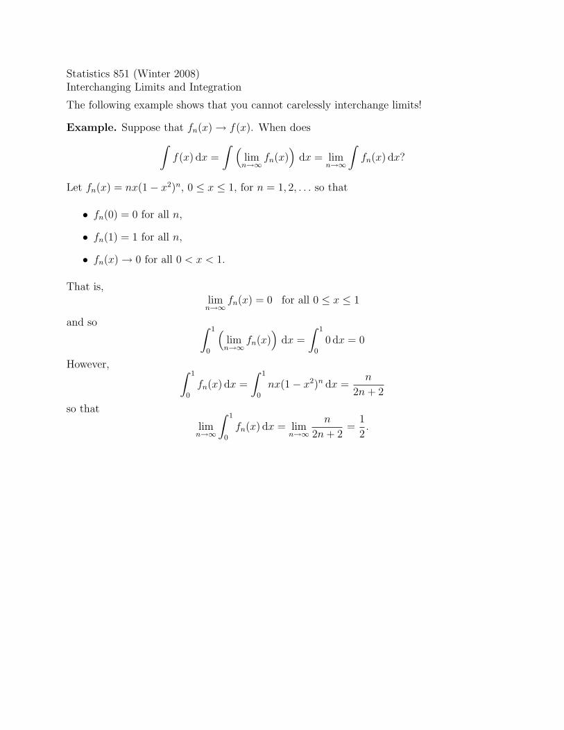
Statistics 851 (Winter 2008)Interchanging Limits and Integration
The following example shows that you cannot carelessly interchange limits!
Example. Suppose that fn(x) → f(x). When does∫f(x) dx =
∫ (lim
n→∞fn(x)
)dx = lim
n→∞
∫fn(x) dx?
Let fn(x) = nx(1− x2)n, 0 ≤ x ≤ 1, for n = 1, 2, . . . so that
• fn(0) = 0 for all n,
• fn(1) = 1 for all n,
• fn(x) → 0 for all 0 < x < 1.
That is,lim
n→∞fn(x) = 0 for all 0 ≤ x ≤ 1
and so ∫ 1
0
(lim
n→∞fn(x)
)dx =
∫ 1
0
0 dx = 0
However, ∫ 1
0
fn(x) dx =
∫ 1
0
nx(1− x2)n dx =n
2n + 2
so that
limn→∞
∫ 1
0
fn(x) dx = limn→∞
n
2n + 2=
1
2.

Statistics 851 (Winter 2008) February 13, 2008Prof. Michael Kozdron
Lecture #17: Comparison of Lebesgue and Riemann Integrals
Reference. Today’s notes!
The purpose of today’s lecture is to compare the Lebesgue integral with the Riemann integral.
In order to illustrate the differences between the two, we will not use probability notation,but instead use calculus notation.
Consider the probability space (Ω,A, P ) where Ω = [0, 1], A denotes the Borel sets of [0, 1],and P denotes the uniform probability on [0, 1]. Let X : Ω → R be a random variable andconsider the expectation of X given by∫
Ω
X(ω) P (dω). (∗)
The uniform probability measure on [0, 1] is sometimes called Lebesgue measure and is de-noted by µ. Instead of using ω ∈ [0, 1] we will use x ∈ [0, 1], and instead of writingX : [0, 1] → R for a random variable we will write h : [0, 1] → R for a measurable function.Therefore, in our new language, (∗) is equivalent to∫
[0,1]
h(x) µ(dx) =
∫ 1
0
h(x) µ(dx)
which we call the Lebesgue integral of h.
By using this notation, we immediately see the analogy with∫ 1
0
h(x) dx,
the Riemann integral of h.
If we translate back to the language of probability, the Riemann integral of the randomvariable X would be written as ∫
Ω
X(ω) dω.
Example. Suppose that h(x) = 1Q1(x) is the indicator function of the rational numbers in[0, 1]. That is,
h(x) =
1, if x ∈ [0, 1] ∩Q,
0, if x 6∈ [0, 1] ∩Q.
Note that h is a simple function; that is, we can write
h(x) =2∑
i=1
ai1Ai(x)
17–1

where a1 = 1, a2 = 0, A1 = [0, 1] ∩ Q, and A2 = [0, 1] ∩ Qc. By definition, the Lebesgueintegral of h is∫ 1
0
h(x) µ(dx) =2∑
i=1
aiµ(Ai) = 1 · µ(A1) + 0 · µ(A2) = µ(A1) = 0
since A1 is a countable set.
Suppose that we now try to compute the Riemann integral∫ 1
0
h(x) dx.
If h has an antiderivative, then we can use the Fundamental Theorem of Calculus. Thetrouble is that h is discontinuous everywhere and so h cannot possibly have an antiderivative.Therefore, in order to compute the Riemann integral we must resort to using the definition.
Definition. Suppose that P = 0 = x0 < x1 < x2 < · · · < xN−1 < xN = 1 is a partition of[0, 1], and let ∆xi = xi+1−xi for i = 0, 1, . . . , N − 1. The function h : [0, 1] → R is Riemannintegrable if
limN→∞
N−1∑i=0
h(x∗i )∆xi
exists for all choices of partitions P and x∗i ∈ [xi, xi+1]. If so, we write∫ 1
0
h(x) dx = limN→∞
N−1∑i=0
h(x∗i )∆xi
for the common value of this limit.
Example (continued). We will make our first attempt to compute∫ 1
0
h(x) dx.
Let
P =
0,
1
N,
2
N, . . . ,
N − 1
N, 1
so that
∆xi =1
N.
For i = 0, 1, . . . , N − 1, let
x∗i =i
N+
1
2N
and note that x∗i is always rational. Therefore, by the definition of h we have
h(x∗i ) = 1
17–2
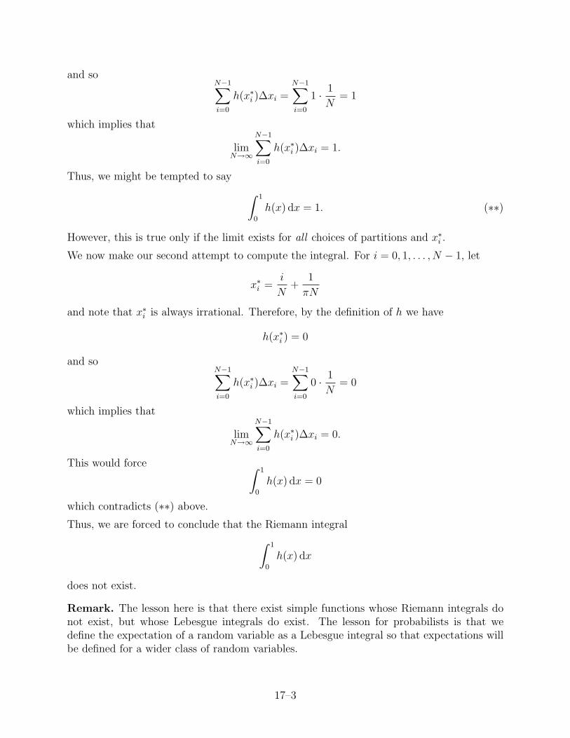
and soN−1∑i=0
h(x∗i )∆xi =N−1∑i=0
1 · 1
N= 1
which implies that
limN→∞
N−1∑i=0
h(x∗i )∆xi = 1.
Thus, we might be tempted to say ∫ 1
0
h(x) dx = 1. (∗∗)
However, this is true only if the limit exists for all choices of partitions and x∗i .
We now make our second attempt to compute the integral. For i = 0, 1, . . . , N − 1, let
x∗i =i
N+
1
πN
and note that x∗i is always irrational. Therefore, by the definition of h we have
h(x∗i ) = 0
and soN−1∑i=0
h(x∗i )∆xi =N−1∑i=0
0 · 1
N= 0
which implies that
limN→∞
N−1∑i=0
h(x∗i )∆xi = 0.
This would force ∫ 1
0
h(x) dx = 0
which contradicts (∗∗) above.
Thus, we are forced to conclude that the Riemann integral∫ 1
0
h(x) dx
does not exist.
Remark. The lesson here is that there exist simple functions whose Riemann integrals donot exist, but whose Lebesgue integrals do exist. The lesson for probabilists is that wedefine the expectation of a random variable as a Lebesgue integral so that expectations willbe defined for a wider class of random variables.
17–3

Statistics 851 (Winter 2008) February 15, 2008Prof. Michael Kozdron
Lecture #18: An Example of a Random Variable with aNon-Borel Range
Suppose that (Ω,A, P ) is a probability space and let X : Ω → R be a random variable.
Recall that the notation X : Ω → R means that the domain of X is Ω and the co-domainof X is R. The function X is necessarily defined for every ω ∈ Ω. However, there is norequirement that X be onto R. We write X(Ω) for the range of R so that X(Ω) ⊆ R.
Also recall that the condition for the function X : Ω → R to be a random variable is thatthe inverse image of a Borel set be an event. That is, we must have X−1(B) ∈ A for everyB ∈ B.
The question might now be asked why we need to consider “inverse images” of Borel sets.Why is not enough to consider “images” of events in A under X?
Notice that we necessarily must have X−1(R) = Ω for every real-valued function X : Ω → R.In particular, this is true whether or not X is measurable.
However, it need not be the case that X(Ω) = R. Again, it is the case that the range of Xis all of R if and only if X is onto R.
Example. For instance, suppose that Ω = [0, 1] and consider the two functions X : Ω → Rand Y : Ω → R given by
X(ω) = ω
and
Y (ω) =
0, if ω = 0,
− 14ω
, if 0 < ω < 14,
12−4ω
, if 14≤ ω < 1
2,
4ω − 3, if 12≤ ω ≤ 1.
It is not hard to show that both X and Y are random variables with respect to the uniformprobability measure on (Ω,B(Ω)). However, X(Ω) = [0, 1] ( R while Y (Ω) = R.
As we have already noted, it is necessarily the case that the range of X satisfies X(Ω) ⊆ R.Hence, it is natural to ask whether or not X(Ω) ∈ B.
However, as the following example shows, it need not be the case that X(Ω) ∈ B even if Xis a random variable.
Example. Suppose that H ⊂ [0, 1] is a non-measurable set and let q ∈ H be a given point.Recall from Lecture #9 that the construction of H and the identification of q requires theAxiom of Choice.
Let Ω = H and let A = 2Ω be the power set of Ω. For A ∈ A, let
PA =
1, if q ∈ A,
0, if q 6∈ A,
18–1

so that P is, in fact, a probability measure on A. Define the function X : Ω → R bysetting X(ω) = ω. If B ∈ B is a Borel set, then X−1(B) ⊂ Ω so that we necessarily haveX−1(B) ∈ A. In other words, X is a random variable. However, it is clearly the case thatX(Ω) = H so that X(Ω) 6∈ B.
We end by proving a related result; namely, the fact that if X : (Ω,A) → (R,B) is a randomvariable, then X−1(B) is a σ-algebra.
Proposition. If F = X−1(B) = X−1(B) : for some B ∈ B, then F is a σ-algebra.
Proof. In order to prove that F is a σ-algebra, we need to verify that the three conditionsin the definition are met.
(i) Since B is a σ-algebra, we know that ∅ ∈ B. However, it then follows that ∅ = X−1(∅) ∈ F .
(ii) Suppose that A ∈ F so that A = X−1(B) for some B ∈ B. However, Ac = [X−1(B)]c =X−1(Bc). Since B is a σ-algebra, we know that Bc ∈ B and so Ac ∈ F . In particular,combining this with (i) implies that Ω = ∅c ∈ F .
(iii) Suppose that A1, A2, . . . ∈ F so that Ai = X−1(Bi), i = 1, 2, . . ., for some B1, B2, . . . ∈ B.However,
∞⋃i=1
Ai =∞⋃i=1
X−1(Bi) = X−1
(∞⋃i=1
Bi
).
Since B is a σ-algebra, we know that
∞⋃i=1
Bi ∈ B
and so∞⋃i=1
Ai ∈ F .
Thus, F is, in fact, a σ-algebra.
The σ-algebra given in the previous proposition is important enough to have its own name.
Definition. Suppose that X : (Ω,A) → (R,B) is a random variable. The σ-algebra gener-ated by X is defined to be σ(X) = X−1(B).
Remark. Notice that the previous proposition never actually used the fact that X is arandom variable. This result is true for any function X : Ω → (R,B).
Remark. In Exercise 9.1 you are asked to show that if X : (Ω,A) → (R,B) is a randomvariable, then it is also measurable as a function from (Ω, σ(X)) → (R,B). In this case, wehave σ(X) ⊆ A.
However, if X : Ω → R is any function, then, although X is necessarily measurable as afunction from (Ω, σ(X)) → (R,B), it is no longer true that σ(X) ⊆ A.
18–2
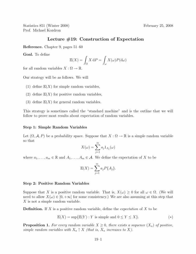
Statistics 851 (Winter 2008) February 25, 2008Prof. Michael Kozdron
Lecture #19: Construction of Expectation
Reference. Chapter 9, pages 51–60
Goal. To define
E(X) =
∫Ω
X dP =
∫ω
X(ω)P (dω)
for all random variables X : Ω → R.
Our strategy will be as follows. We will
(1) define E(X) for simple random variables,
(2) define E(X) for positive random variables,
(3) define E(X) for general random variables.
This strategy is sometimes called the “standard machine” and is the outline that we willfollow to prove most results about expectation of random variables.
Step 1: Simple Random Variables
Let (Ω,A, P ) be a probability space. Suppose that X : Ω → R is a simple random variableso that
X(ω) =m∑
j=1
aj1Aj(ω)
where a1, . . . , am ∈ R and A1, . . . , Am ∈ A. We define the expectation of X to be
E(X) =m∑
j=1
ajPAj.
Step 2: Positive Random Variables
Suppose that X is a positive random variable. That is, X(ω) ≥ 0 for all ω ∈ Ω. (We willneed to allow X(ω) ∈ [0, +∞] for some consistency.) We are also assuming at this step thatX is not a simple random variable.
Definition. If X is a positive random variable, define the expectation of X to be
E(X) = supE(Y ) : Y is simple and 0 ≤ Y ≤ X. (∗)
Proposition 1. For every random variable X ≥ 0, there exists a sequence (Xn) of positive,simple random variables with Xn ↑ X (that is, Xn increases to X).
19–1

Proof. Let X ≥ 0 be given and define the sequence
Xn(ω) =
k2n , if k
2n ≤ X(ω) < k+12n and 0 ≤ k ≤ n2n − 1,
n, if X(ω) ≥ n.
Then it follows that Xn ≤ Xn+1 for every n = 1, 2, 3, . . . and Xn → X which completes theproof.
Proposition 2. If X ≥ 0 and (Xn) is a sequence of simple random variables with Xn ↑ X,then E(Xn) ↑ E(X). That is, if Xn ≤ Xn+1 and
limn→∞
Xn = X,
then
limn→∞
∫Xn dP ↑
∫ (lim
n→∞Xn
)dP =
∫X dP.
Proof. Suppose that X ≥ 0 is a random variable and let (Xn) be a sequence of simplerandom variables with Xn ≥ 0 and Xn ↑ X. Observe that since the Xn are increasing, wehave E(Xn) ≤ E(Xn+1). Therefore, E(Xn) increases to some limit a ∈ [0,∞]; that is,
E(Xn) ↑ a
for some 0 ≤ a ≤ ∞. (If E(Xn) is an unbounded sequence, then a = ∞. However, if E(Xn)is a bounded sequence, then a < ∞ follows from the fact that increasing, bounded sequenceshave unique limits.) Therefore, it follows from (∗), the definition of E(X), that a ≤ E(X).
We will now show a ≥ E(X). As a result of (∗), we only need to show that if Y is a simplerandom variable with 0 ≤ Y ≤ X, then E(Y ) ≤ a. To this end, let Y be simple and write
Y =m∑
k=1
ak1Y = ak.
That is, take Ak = ω : Y (ω) = ak. Let 0 < ε ≤ 1 and define
Yn,ε = (1− ε)Y 1(1−ε)Y≤Xn.
Note that Yn,ε = (1− ε)ak on the set
(1− ε)Y ≤ Xn ∩ Ak = Ak,n,ε
and that Yn,ε = 0 on the set (1− ε)Y > Xn. Clearly Yn,ε ≤ Xn and so
E(Yn,ε) = (1− ε)m∑
k=1
akPAk,n,ε ≤ E(Xn).
Therefore, sinceY ≤ X = lim
n→∞Xn
19–2

we see that(1− ε)Y < lim
n→∞Xn
as soon as Y > 0. (This requires that X is not identically 0.) Hence,
Ak,n,ε → Ak
as n →∞. By Theorem 2.4 we conclude that
PAk,n,ε → PAkso that
E(Yn,ε) = (1− ε)m∑
k=1
akPAk,n,ε → (1− ε)m∑
k=1
akPAk = (1− ε)E(Y ) ≤ a.
That is,E(Yn,ε) ≤ E(Xn)
andE(Yn,ε) → (1− ε)E(Y ) and E(Xn) → a
so that(1− ε)E(Y ) ≤ a
(which follows since everything is increasing). Let ε > 0 so that
E(Y ) ≤ a.
By (∗),supE(Y ) ≤ a
which implies thatE(X) ≤ a.
Combined with our earlier result that a ≤ E(X) we conclude E(X) = a and the proof iscomplete.
Step 3: General Random Variables
Now suppose that X is any random variable. Write
X+ = maxX, 0 and X− = −minX, 0for the positive part and the negative part of X, respectively. Note that X+ ≥ 0 andX− ≥ 0 so that the positive part and negative part of X are both positive random variablesand X = X+ −X−.
Definition. A random variable X is called integrable (or has finite expectation) if bothE(X+) and E(X−) are finite. In this case we define E(X) to be
E(X) = E(X+)− E(X−).
Remark. Having proved this result, we see that the standard machine is really not that hardto implement. In fact, it is usually enough to prove a result for simple random variables andthen extend that result to positive random variables using the result of Step 2. Step 3 forgeneral random variables usually follows by definition.
19–3
Statistics 851 (Winter 2008) February 27, 2008Prof. Michael Kozdron
Lecture #20: Independence
Reference. Chapter 10, pages 65–67
Let (Ω,A, P ) be a probability space. Recall that events A ∈ A and B ∈ A are independentif
PA ∩B = PA · PB.
We can extend this idea to collections of events as follows.
Definition. Two sub-σ-algebras A1 ⊆ A and A2 ⊆ A are independent if
PA1 ∩ A2 = PA1 · PA2
for every A1 ∈ A1 and A2 ∈ A2.
Furthermore, a collection (Ai), i ∈ I, of sub-σ-algebras of A is independent if for every finitesubset J of I, we have
P
⋂i∈J
Ai
=∏i∈J
PAi
for all Ai ∈ Ai.
We can now discuss independent random variables.
Recall. Suppose that (E, E) is a measurable space. The function X : (Ω,A) → (E, E) iscalled measurable if X−1(B) ∈ A for every B ∈ E . Usually we take (E, E) = (R,B) and callX a random variable.
Now, as shown in Lecture #18,
X−1(E) = A ∈ A : X(A) = B for some B ∈ E
is a σ-algebra with X−1(E) ⊆ A.
This sub-σ-algebra is so important that it gets its own name and notation.
Notation. We write σ(X) to denote the σ-algebra generated by X. In other words, σ(X) =X−1(E).
Definition. Suppose that (E, E) and (F,F) are measurable spaces, and let X : (Ω,A) →(E, E) and Y : (Ω,A) → (F,F) be random variables. We say that X and Y are indpendentif σ(X) and σ(Y ) are independent σ-algebras.
Notice that both σ(X) and σ(Y ) are sub-σ-algebras of A even though X and Y might havedifferent target spaces.
20–1
Theorem. The random variables X and Y are independent if and only if
PX ∈ A, Y ∈ B = PX ∈ A · PY ∈ B
for all A ∈ E and B ∈ F .
Proof. This follows from the definition of σ(X) since X−1(E) is exactly the σ-algebra gener-ated by events of the form X ∈ A for A ∈ E . That is,
σ(X) = σ(X ∈ A, A ∈ E) and σ(Y ) = σ(Y ∈ B, B ∈ F)
and so the theorem follows.
Corollary. The random variables X and Y are independent if and only if
PX,Y A, B = PXA · P Y B
where PX,Y denotes the joint law of X and Y .
Corollary. The random variables X and Y are independent if and only if
FX,Y (x, y) = FX(x) · FY (y)
where FX,Y denotes the joint distribution function of X and Y .
Corollary. If the random variables X and Y have densities fX and fY , respectively, andjoint density fX,Y , then X and Y are independent if and only if
fX,Y (x, y) = fX(x) · fY (y).
Remark. We still need to define the terms joint law, joint distribution function, and jointdensity function. This will require the notion of product spaces.
Theorem. If X and Y are independent random variables, and if f and g are measurablefunctions, then f X and g Y are independent random variables.
Proof. Given f and g we have
(f X)−1(E) = X−1(f−1(E)) ⊆ X−1(E)
and(g Y )−1(F) = Y −1(g−1(F)) ⊆ Y −1(F).
If X and Y are independent, then X−1(E) and Y −1(F) are independent so that X−1(f−1(E))and Y −1(g−1(F)) are independent. That is,
σ(f X) and σ(g Y )
are independent and the proof is complete.
20–2
Theorem. If X and Y are independent random variables, then
E(f(X)g(Y )) = E(f(X)) · E(g(Y )) (∗)
for every pair of bounded, measurable functions f , g, or positive, measurable functions f , g.
Remark. If X and Y are jointly continuous random variables, then this result is easilyproved as in STAT 351:∫ ∞
−∞
∫ ∞
−∞f(x)g(y)fX,Y (x, y) dx dy =
∫ ∞
−∞
∫ ∞
−∞f(x)g(y)fX(x)fY (y) dx dy
=
∫ ∞
−∞f(x)fX(x) dx ·
∫ ∞
−∞g(y)fY (y) dy.
Proof. In order to prove this result, we follow that standard machine. Suppose that X andY are random variables and that f and g are measurable functions. The first step is to showthat the result holds when f and g are simple functions. Suppose that f(x) = 1A(x) andg(y) = 1B(y). Then,
E(f(X)g(Y )) = E(1A(X)1B(Y )) = E(1X ∈ A, Y ∈ B)= PX ∈ A, Y ∈ B= PX ∈ A · PY ∈ B= E(1A(X)) · E(1B(Y ))
= E(f(X)) · E(g(Y )).
If
f(x) =n∑
i=1
ai1Ai(x) and g(y) =
m∑j=1
bj1Bj(y),
then the result (∗) holds by linearity.
The second step is to show that the result holds for positive functions. Thus, let f , g bepositive functions and assume that fn and gn are sequences of positive, simple functions withfn ↑ f and gn ↑ g. Note that
fn(x) · gn(y) ↑ f(x) · g(y).
Therefore,
E(f(X) · g(Y )) = E(
limn→∞
fn(X) · gn(Y ))
= limn→∞
E(fn(X) · gn(Y )) by the Monotone Convergence Theorem
= limn→∞
[E(fn(X)) · E(gn(Y ))] by Step 1
= limn→∞
E(fn(X)) · limn→∞
E(gn(Y ))
= E(
limn→∞
fn(X))· E(
limn→∞
gn(Y ))
by the Monotone Convergence Theorem
= E(f(X)) · E(g(Y )).
20–3

The third step is to conclude that if f , g are both bounded, then the result follows by writing
f = f+ − f− and g = g+ − g−
and using linearity.
20–4

Statistics 851 (Winter 2008) February 29, 2008Prof. Michael Kozdron
Lecture #21: Product Spaces
Reference. Chapter 10, pages 67–71
We begin with the following result which gives a characterization of independent σ-algebrasin terms of the probabilities of the events.
Theorem. Suppose that (Ω,A, P ) is a probability space. The σ-algebra A is independent ofitself if and only if PA ∈ 0, 1 for all A ∈ A.
Proof. Suppose that A is independent of itself. This implies that PA∩B = PA ·PBfor every A, B ∈ A. In particular, let A ∈ A so that Ac ∈ A. Therefore,
0 = P∅ = PA ∩ Ac = PA · PAc
which can only be satisfied if either PA = 0 or PAc = 0. That is, we must havePA ∈ 0, 1.Conversely, suppose that PA ∈ 0, 1 for all A ∈ A. If A, B ∈ A, then there are threecases that need to be considered.
(i) Suppose that PA = PB = 0. Therefore, since
0 ≤ PA ∩B ≤ PA = 0
we conclude thatPA ∩B = PA · PB (= 0).
(ii) Suppose that PA = 0 and PB = 1. Therefore, since
0 ≤ PA ∩B ≤ PA = 0
we again conclude thatPA ∩B = PA · PB (= 0).
(Similarly, we reach the same conclusion if PA = 1 and PB = 0.)
(iii) Suppose that PA = PB = 1. Therefore,
0 ≤ P(A ∩B)c = PAc ∪Bc ≤ PAc+ PBc = 0
which implies that PA ∩B = 1 and so
PA ∩B = PA · PB (= 1).
Thus we have demonstrated both implications, the theorem is proved.
21–1
An equivalent formulation of the theorem is given by the contrapositive.
Theorem. The σ-algebra A is not independent of itself if and only if there exists an A ∈ Awith PA ∈ (0, 1).
Remark. Therefore, suppose that (Ω,A, P ) is a probability space and suppose that A1
and A2 are two sub-σ-algebras of A. It is possible to discuss the independence (or non-independence) of A1 and A2 even if A1 = A2.
As indicated last class, it is necessary to talk about joint distributions. In order to do so,however, we must define product spaces.
Let X : (Ω,A) → (E, E) be a random variable and let Y : (Ω,A) → (F,F) be a randomvariable.
Definition. If E and F are sets, then we write
E × F = (x, y) : x ∈ E, y ∈ F
for their Cartesian product.
Consider the function Z : Ω → E × F given by
ω 7→ Z(ω) = (X(ω), Y (ω)).
It should seem “obvious” that Z is a random variable. However, in order to prove thatZ : Ω → E × F is, in fact, measurable, we need to have a σ-algebra on E × F .
If E and F are σ-algebras, then
E × F = A ⊂ E × F : A = Λ× Γ, Λ ∈ E , Γ ∈ F
is well-defined although it need not be a σ-algebra. Let
σ(E ,F) = E ⊗ F
denote the smallest σ-algebra containing both E and F .
Hence, (E×F, E⊗F) is also a measurable space, and this leads us to the following definition.
Definition. A function f : (E × F, E ⊗ F) → (R,B) is measurable if f−1(B) ∈ E ⊗ F forevery B ∈ B.
Suppose further that P1 is a probability on (E, E) and that P2 is a probability on (F,F). Isit possible to define a probability P on (E × F, E ⊗ F) in a natural way?
Answer. YES!
Intuition. Let C ∈ E × F so that C = A × B. We should define the probability PC =P1A · P2B. That is, we should define the probability of the product as the product ofthe probabilities. The problem, however, is that E ×F need not equal E ⊗F . That is, thereare events C ∈ E ⊗F which are NOT of the form C = A×B for some A ∈ E , B ∈ F . Howshould we define P for these sets? The answer will be given by the Fubini-Tonelli Theorem.
21–2

Statistics 851 (Winter 2008)Exercises on Independence
Suppose that (Ω,A, P ) is a probability space with Ω = a, b, c, d, e and A = 2Ω. Let X andY be the real-valued random variables defined by
X(ω) =
1, if ω ∈ a, b,0, if ω 6∈ a, b,
Y (ω) =
2, if ω ∈ a, c,0, if ω 6∈ a, c.
(a) Give explicitly (by listing all the elements) the σ-algebras σ(X) and σ(Y ) generatedby X and Y , respectively.
(b) Find the σ-algebra σ(X, Y ) generated (jointly) by X and Y .
(c) If Z = X + Y , does σ(Z) = σ(X, Y )?
For real numbers α, β ≥ 0 with α + β ≤ 1/2, let P be the probability measure on Adetermined by the relations
P (a) = P (b) = α, P (c) = P (d) = β, P (e) = 1− 2(α + β).
(d) Find all α, β for which σ(X) and σ(Y ) are independent. Simplify!
(e) Find all α, β for which X and Z = X + Y are independent.

Statistics 851 (Winter 2008)Exercises on Independence (Solutions)
Suppose that (Ω,A, P ) is a probability space with Ω = a, b, c, d, e and A = 2Ω. Let X andY be the real-valued random variables defined by
X(ω) =
1, if ω ∈ a, b,0, if ω 6∈ a, b,
Y (ω) =
2, if ω ∈ a, c,0, if ω 6∈ a, c.
(a) Give explicitly (by listing all the elements) the σ-algebras σ(X) and σ(Y ) generatedby X and Y , respectively.
Suppose that B ∈ B so that
X−1(B) =
Ω, if 1 ∈ B, 0 ∈ B,
a, b, if 1 ∈ B, 0 6∈ B,
c, d, e, if 1 6∈ B, 0 ∈ B,
∅, if 1 6∈ B, 0 6∈ B.
Thus, the σ-algebra generated by X is σ(X) = ∅, Ω, a, b, c, d, e. Similarly,
Y −1(B) =
Ω, if 2 ∈ B, 0 ∈ B,
a, c, if 2 ∈ B, 0 6∈ B,
b, d, e, if 2 6∈ B, 0 ∈ B,
∅, if 2 6∈ B, 0 6∈ B.
so that σ(Y ) = ∅, Ω, a, c, b, d, e.
(b) Find the σ-algebra σ(X, Y ) generated (jointly) by X and Y .
By definition,
σ(X,Y ) = σ(σ(X), σ(Y )) = σ(a, b, c, d, e)= ∅, Ω, a, b, c, d, e, a, b, a, c, a, d, e, b, c, b, d, ec, d, e, a, b, c,
a, b, d, e, a, c, d, e, b, c, d, e .
(c) If Z = X + Y , does σ(Z) = σ(X, Y )?
If Z = X + Y then
Z(ω) =
3, if ω = a
2, if ω = c
1, if ω = b
0, if ω ∈ d, eso that
σ(Z) = σ(a, b, c, d, e) = σ(X, Y ).
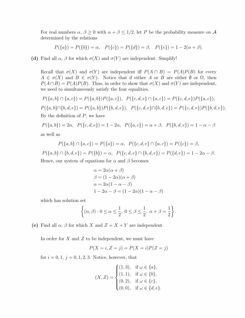
For real numbers α, β ≥ 0 with α + β ≤ 1/2, let P be the probability measure on Adetermined by the relations
P (a) = P (b) = α, P (c) = P (d) = β, P (e) = 1− 2(α + β).
(d) Find all α, β for which σ(X) and σ(Y ) are independent. Simplify!
Recall that σ(X) and σ(Y ) are independent iff P (A ∩ B) = P (A)P (B) for everyA ∈ σ(X) and B ∈ σ(Y ). Notice that if either A or B are either ∅ or Ω, thenP (A∩B) = P (A)P (B). Thus, in order to show that σ(X) and σ(Y ) are independent,we need to simultaneously satisfy the four equalities.
P (a, b ∩ a, c) = P (a, b)P (a, c), P (c, d, e ∩ a, c) = P (c, d, e)P (a, c),
P (a, b∩b, d, e) = P (a, b)P (b, d, e), P (c, d, e∩b, d, e) = P (c, d, e)P (b, d, e).By the definition of P , we have
P (a, b) = 2α, P (c, d, e) = 1− 2α, P (a, c) = α + β, P (b, d, e) = 1− α− β
as well as
P (a, b ∩ a, c) = P (a) = α, P (c, d, e ∩ a, c) = P (c) = β,
P (a, b ∩ b, d, e) = P (b) = α, P (c, d, e ∩ b, d, e) = P (d, e) = 1− 2α− β.
Hence, our system of equations for α and β becomes
α = 2α(α + β)
β = (1− 2α)(α + β)
α = 2α(1− α− β)
1− 2α− β = (1− 2α)(1− α− β)
which has solution set(α, β) : 0 ≤ α ≤ 1
2, 0 ≤ β ≤ 1
2, α + β =
1
2
.
(e) Find all α, β for which X and Z = X + Y are independent.
In order for X and Z to be independent, we must have
P (X = i, Z = j) = P (X = i)P (Z = j)
for i = 0, 1, j = 0, 1, 2, 3. Notice, however, that
(X, Z) =
(1, 3), if ω ∈ a,(1, 1), if ω ∈ b,(0, 2), if ω ∈ c,(0, 0), if ω ∈ d, e.
These imply that
P (a) = P (a, b)P (a), P (b) = P (a, b)P (b),
P (c) = P (c, d, e)P (c), P (d, e) = P (c, d, eP (d, e)
which are simultaneously satisfied by either (α = 1/2, β = 0) or (α = 0, β = 0).
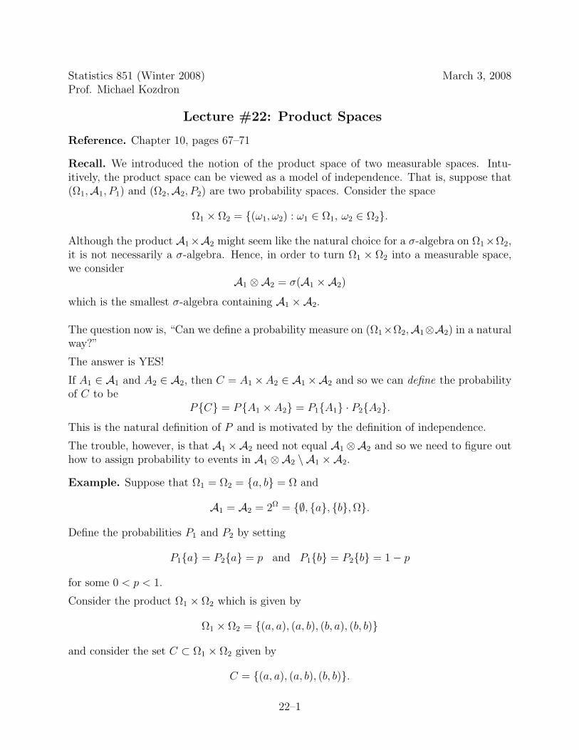
Statistics 851 (Winter 2008) March 3, 2008Prof. Michael Kozdron
Lecture #22: Product Spaces
Reference. Chapter 10, pages 67–71
Recall. We introduced the notion of the product space of two measurable spaces. Intu-itively, the product space can be viewed as a model of independence. That is, suppose that(Ω1,A1, P1) and (Ω2,A2, P2) are two probability spaces. Consider the space
Ω1 × Ω2 = (ω1, ω2) : ω1 ∈ Ω1, ω2 ∈ Ω2.
Although the product A1×A2 might seem like the natural choice for a σ-algebra on Ω1×Ω2,it is not necessarily a σ-algebra. Hence, in order to turn Ω1 × Ω2 into a measurable space,we consider
A1 ⊗A2 = σ(A1 ×A2)
which is the smallest σ-algebra containing A1 ×A2.
The question now is, “Can we define a probability measure on (Ω1×Ω2,A1⊗A2) in a naturalway?”
The answer is YES!
If A1 ∈ A1 and A2 ∈ A2, then C = A1 ×A2 ∈ A1 ×A2 and so we can define the probabilityof C to be
PC = PA1 × A2 = P1A1 · P2A2.
This is the natural definition of P and is motivated by the definition of independence.
The trouble, however, is that A1 ×A2 need not equal A1 ⊗A2 and so we need to figure outhow to assign probability to events in A1 ⊗A2 \ A1 ×A2.
Example. Suppose that Ω1 = Ω2 = a, b = Ω and
A1 = A2 = 2Ω = ∅, a, b, Ω.
Define the probabilities P1 and P2 by setting
P1a = P2a = p and P1b = P2b = 1− p
for some 0 < p < 1.
Consider the product Ω1 × Ω2 which is given by
Ω1 × Ω2 = (a, a), (a, b), (b, a), (b, b)
and consider the set C ⊂ Ω1 × Ω2 given by
C = (a, a), (a, b), (b, b).
22–1

Note that C is NOT of the form C = A1 ×A2. Therefore, we cannot assign a probability toC by simply defining
PC = P1A1 · P2A2
and so we need to be able to extend P1 × P2 to be a probability on all of A1 ⊗A2.
Finally, note that in this example, which models two independent tosses of a coin, we wouldlike to assign
PC = p2 + p(1− p) + (1− p)2 = 1− p + p2.
Exercise. Explicitly list all of the elements of A1 ×A2 and A1 ⊗A2. Give the probabilityP1 × P2C for all C ∈ A1 ×A2. Define PC (in a consistent way) for all C ∈ A1 ⊗A2 \A1 ×A2.
Random Vectors
We begin with the following result given in Exercise 10.1 which shows that (X1, X2) is arandom vector if and only if X1 and X2 are both random variables.
Theorem. Let (Ω,A, P ) be a probability space and suppose that X = (X1, X2) : Ω → E×F .The function X : (Ω,A) → (E×F, E ⊗F) is measurable if and only if X1 : (Ω,A) → (E, E)and X2 : (Ω,A) → (F,F) are measurable.
Proof. Suppose that both X1 : (Ω,A) → (E, E) and X2 : (Ω,A) → (F,F) are measurable.Let A ∈ E , B ∈ F , so that X−1
1 (A) ∈ A and X−12 (B) ∈ A by the measurability of X1, X2,
respectively. Therefore,
X−1(A×B) = X−11 (A) ∩X−1
2 (B) ∈ A
so that X is measurable by the definition of the product σ-algebra E ⊗ F and Theorem 8.1(since E ⊗ F is generated by E × F = A×B : A ∈ E , B ∈ F).Conversely, suppose that X = (X1, X2) : Ω → E × F is measurable so that X−1(C) ∈ A forevery C ∈ E ⊗ F . In particular, X−1(C) ∈ A for every C ∈ E × F . If C ∈ E × F , then it isnecessarily of the form A×B for some A ∈ E and some B ∈ F , and so
X−1(C) = X−1(A×B) = X−11 (A) ∩X−1
2 (B) ∈ A. (∗)
In order to show that X1 : (Ω,A) → (E, E) is measurable, we must show X−11 (A) ∈ A for
all A ∈ E . To do this, we simply make a judicious choice of B in (∗). Choosing B = F gives
A 3 X−11 (A) ∩X−1
2 (F ) = X−11 (A) ∩ Ω = X−1
1 (A).
Similarly, to show X2 : (Ω,A) → (F,F) is measurable we choose A = E in (∗). This gives
A 3 X−11 (E) ∩X−1
2 (B) = Ω ∩X−12 (B) = X−1
2 (B).
Taken together, the proof is complete.
22–2

Sections of a measurable function
Suppose that f : (E × F, E ⊗ F) → (R,B) given by
(x, y) 7→ f(x, y) = z
is measurable.
Fix x ∈ E and let fx : F → R be given by
fx(y) = f(x, y).
In other words, we start with a measurable function of two variables, say f(x, y), and viewit as a function of y only for fixed x. Sometimes we will also write
fx(·) = f(x, ·) or y 7→ f(x, y).
Similarly, fix y ∈ F and let fy : E → R be given by
fy(x) = f(x, y).
That is, fy(·) = f(·, y) or x 7→ f(x, y).
We call fx and fy the sections of f .
Remark. There is a similarity between the sections of a measurable function and themarginal densities of a random vector. Suppose that (X, Y ) is a random vector with jointdensity function f(x, y). The sections of f are the functions fx(y) and fy(x) obtained simplyby viewing f(x, y) as a function of a single variable. The marginal densities, however, areobtained by “integrating out” the other variable. That is,
fX(x) =
∫ ∞
−∞f(x, y) dy
is the marginal density function of X and
fY (y) =
∫ ∞
−∞f(x, y) dx
is the marginal density function of Y .
Theorem. If f : (E × F, E ⊗ F) → (R,B) is measurable, then the section fx : F → R isF-measurable and the section fy : E → R is E-measurable.
Remark. The converse is false in general.
Proof. We will apply the standard machine and show that fx is F -measurable. (The proofthat fy is E-measurable is identical.)
Let f(x, y) = 1C(x, y) for C ∈ E ⊗ F and let
H = C ∈ E ⊗ F : y 7→ 1C(x, y) is F -measurable for each fixed x ∈ E.
22–3
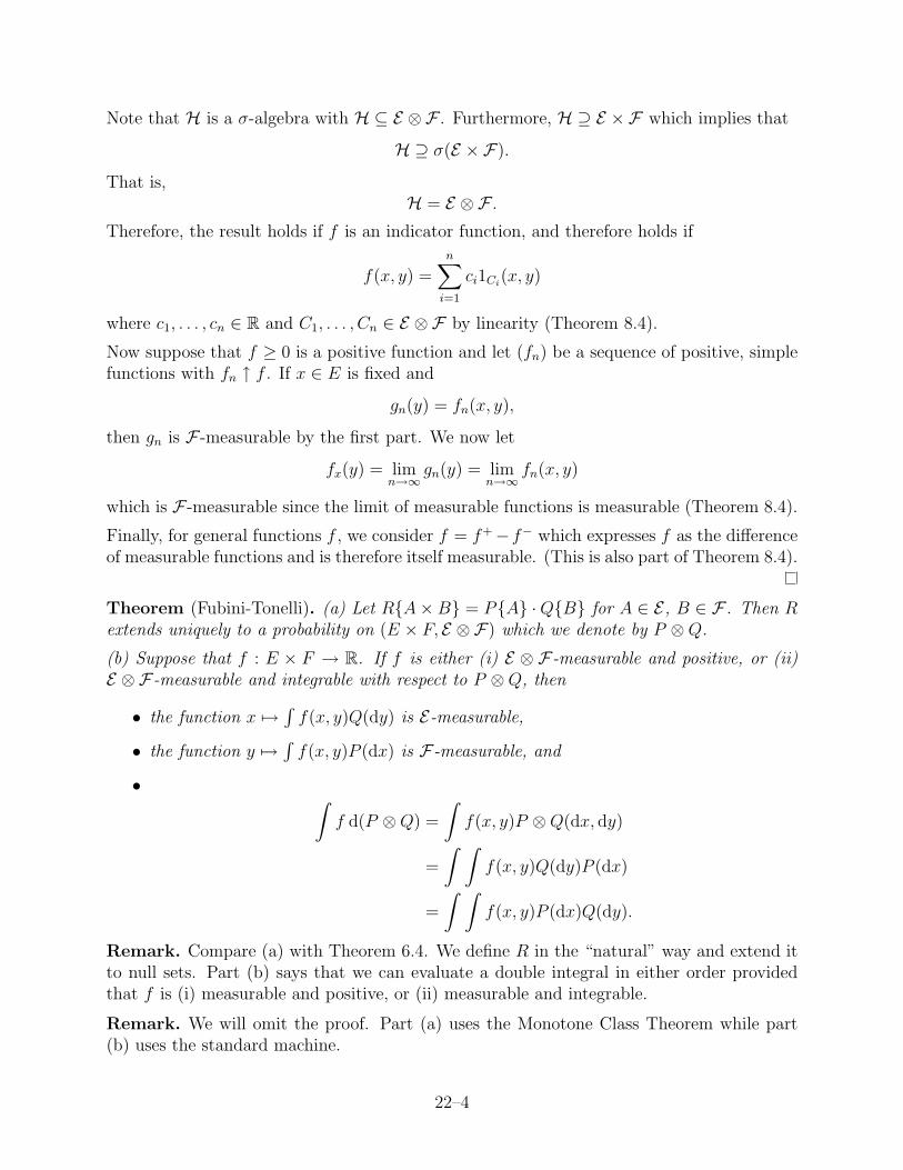
Note that H is a σ-algebra with H ⊆ E ⊗ F . Furthermore, H ⊇ E × F which implies that
H ⊇ σ(E × F).
That is,H = E ⊗ F .
Therefore, the result holds if f is an indicator function, and therefore holds if
f(x, y) =n∑
i=1
ci1Ci(x, y)
where c1, . . . , cn ∈ R and C1, . . . , Cn ∈ E ⊗ F by linearity (Theorem 8.4).
Now suppose that f ≥ 0 is a positive function and let (fn) be a sequence of positive, simplefunctions with fn ↑ f . If x ∈ E is fixed and
gn(y) = fn(x, y),
then gn is F -measurable by the first part. We now let
fx(y) = limn→∞
gn(y) = limn→∞
fn(x, y)
which is F -measurable since the limit of measurable functions is measurable (Theorem 8.4).
Finally, for general functions f , we consider f = f+− f− which expresses f as the differenceof measurable functions and is therefore itself measurable. (This is also part of Theorem 8.4).
Theorem (Fubini-Tonelli). (a) Let RA×B = PA ·QB for A ∈ E, B ∈ F . Then Rextends uniquely to a probability on (E × F, E ⊗ F) which we denote by P ⊗Q.
(b) Suppose that f : E × F → R. If f is either (i) E ⊗ F-measurable and positive, or (ii)E ⊗ F-measurable and integrable with respect to P ⊗Q, then
• the function x 7→∫
f(x, y)Q(dy) is E-measurable,
• the function y 7→∫
f(x, y)P (dx) is F-measurable, and
• ∫f d(P ⊗Q) =
∫f(x, y)P ⊗Q(dx, dy)
=
∫ ∫f(x, y)Q(dy)P (dx)
=
∫ ∫f(x, y)P (dx)Q(dy).
Remark. Compare (a) with Theorem 6.4. We define R in the “natural” way and extend itto null sets. Part (b) says that we can evaluate a double integral in either order providedthat f is (i) measurable and positive, or (ii) measurable and integrable.
Remark. We will omit the proof. Part (a) uses the Monotone Class Theorem while part(b) uses the standard machine.
22–4

Statistics 851 (Winter 2008) March 5, 2008Prof. Michael Kozdron
Lecture #23: The Fubini-Tonelli Theorem
Reference. Chapter 10, pages 67–71
We begin by recalling the Fubini-Tonelli Theorem which gives us conditions under which wecan interchange the order of Lebesgue integration:∫ ∫
f(x, y)Q(dy)P (dx) =
∫ ∫f(x, y)P (dx)Q(dy). (∗)
Formally, suppose that (E, E , P ) and (F,F , Q) are measure spaces and consider the productspace (E × F, E ⊗ F , P ⊗Q). Let f : E × F → R be a function.
The theorem states that equality holds in (∗) if f is either (i) E⊗F -measurable and positive,or (ii) E ⊗ F -measurable and integrable with respect to P ⊗Q.
We also recall the following theorem which tells us that joint measurability of f(x, y) impliesmeasurability of the sections fx(y) and fy(x).
Theorem. If f : (E × F, E ⊗ F) → (R,B) is measurable, then for fixed x ∈ E the sectionfx : F → R given by fx(y) = f(x, y) is F-measurable, and for fixed y ∈ F the sectionfy : E → R given by fx(y) = f(x, y) is E-measurable.
Recall. If f is continuous, then f is measurable. (In fact, if f is continuous almost surely,then f is measurable.)
Example. Suppose that E = [0, 2], E = B(E), P is the uniform probability on E, andsuppose further than F = [0, 1], F = B(F ), Q is the uniform probability on F .
Consider the function
f(x, y) =
xy(x2−y2)(x2+y2)3
, if (x, y) 6= (0, 0),
0, if (x, y) = (0, 0).
It is clear that f is E ⊗ F -measurable since the only possible point of discontinuity is at(0, 0).
Fix x ∈ [0, 2] and consider the section fx(y). For instance, if x = 1, then
fx=1(y) =y(1− y2)
(1 + y2)3for y ∈ [0, 1].
Clearly fx=1(y) is continuous (and hence measurable) for y ∈ [0, 1] = F . Or, for instance,suppose that x = 0. Then fx=0(y) = 0 for y ∈ [0, 1]. In general, for fixed x ∈ (0, 2],
fx(y) =xy(x2 − y2)
(x2 + y2)3, y ∈ [0, 1],
23–1

is continuous for y ∈ F and hence is F -measurable.
Fix y ∈ [0, 1] and consider the section fy(x). For instance, if y = 1/2, then
fy=1/2(x) =x(x2 − 1/4)
2(x2 + 1/4)3for x ∈ [0, 2]
is continuous in x and so fy=1/2(x) is E-measurable. Or, for instance, suppose that y = 0.Then fy=0(x) = 0 for x ∈ [0, 2]. In general, for fixed y ∈ (0, 1],
fy(x) =xy(x2 − y2)
(x2 + y2)3, x ∈ [0, 2],
is continuous for x ∈ E and hence is E-measurable.
We now calculate∫F
f(x, y)Q(dy) =
∫ 1
0
f(x, y)Q(dy) =
∫ 1
0
f(x, y) dy =x
2(x2 + 1)2
which follows since Q is the uniform probability on [0, 1]. Hence,∫E
∫F
f(x, y)Q(dy)P (dx) =
∫E
x
2(x2 + 1)2P (dx) =
∫ 2
0
x
2(x2 + 1)2· 1
2dx = −1
8
(1
x2 + 1
) ∣∣∣∣20
=1
10
which follows since P is the uniform probability on [0, 2].
On the other hand, ∫E
f(x, y)P (dx) =
∫ 2
0
f(x, y) · 1
2dx = − y
2(4 + y2)2
and so∫F
∫E
f(x, y)P (dx)Q(dy) =
∫F
− y
2(4 + y2)2Q(dy) = −
∫ 1
0
y
2(4 + y2)2dy =
1
2
(1
4 + y2
) ∣∣∣∣10
= − 1
40.
The reason that ∫ ∫f(x, y)Q(dy)P (dx) 6=
∫ ∫f(x, y)P (dx)Q(dy)
has to do with f itself. Notice that
f(2t, t) =6
125t2and f(t, 2t) = − 6
125t2.
In order for Fubini-Tonelli to work, it must be the case that f is either
23–2
(i) E ⊗ F -measurable and positive, or
(ii) E ⊗ F -measurable and P ⊗Q-integrable.
Since we have shown that the order of integration does matter for f(x, y), we can concludethat f violates both (i) and (ii). In particular, f is neither positive nor P ⊗Q-integrable. Aswe noted above f is E⊗F -measurable and so this example also shows that joint measurabilityalone is not sufficient for integrability.
Tail Events
Reference. Chapter 10, pages 71–72
Let (Ω,A, P ) be a probability space and let An be a sequence of events in A. Define
lim supn→∞
An =∞⋂
n=1
⋃m≥n
Am = limn→∞
∞⋃m=n
Am
which can be interpreted probabilistically as
An occur infinitely often = An i.o..
Theorem (Borel-Cantelli). Let An be a sequence of events in (Ω,A, P ).
(a) If∞∑
n=1
PAn < ∞,
then PAn i.o. = 0.
(b) If PAn i.o. = 0 and An are mutually independent, then
∞∑n=1
PAn < ∞.
Remark. An equivalent formulation of (b) is: “If An are mutually independent and if
∞∑n=1
PAn = ∞,
then PAn i.o. = 1.”
Suppose that Xn are all random variables defined on (Ω,A, P ). Define the σ-algebras Bn =σ(Xn) and
Cn = σ(Xn, Xn+1, Xn+2, . . .) = σ
(⋃p≥n
Bp
).
Let
C∞ =∞⋂
n=1
Cn.
23–3
Definition. By Exercise 2.2, we have that C∞ is a σ-algebra which we call the tail σ-algebra(associated to the sequence X1, X2, . . .).
Theorem (Kolmogorov’s Zero-One Law). If Xn are independent random variables and C ∈C∞, then either PC = 0 or PC = 1.
23–4
Statistics 851 (Winter 2008) March 7, 2008Prof. Michael Kozdron
Lecture #24: The Borel-Cantelli Lemma
Reference. Chapter 10, pages 71–72
Let (Ω,A, P ) be a probability space and let An be a sequence of events in A. Define
lim supn→∞
An =∞⋂
n=1
⋃m≥n
Am = limn→∞
∞⋃m=n
Am
which can be interpreted probabilistically as
An occur infinitely often = An i.o..
Theorem (Borel-Cantelli). Let An be a sequence of events in (Ω,A, P ).
(a) If∞∑
n=1
PAn < ∞,
then PAn i.o. = 0.
(b) If PAn i.o. = 0 and An are mutually independent, then
∞∑n=1
PAn < ∞.
Proof. (a) Suppose that an = PAn = E(1An). By Theorem 9.2,
∞∑n=1
PAn =∞∑
n=1
an < ∞
implies∞∑
n=1
1An < ∞ a.s.
However,∞∑
n=1
1An(ω) = ∞
if and only if
ω ∈∞⋂
n=1
⋃m≥n
Am = lim supn→∞
An.
24–1

Together these give∞∑
n=1
PAn < ∞ ⇒ PAn i.o. = 0.
(b) Suppose that An are mutually independent. Then
Plim supn→∞
An = P
∞⋂
n=1
⋃m≥n
Am
= limn→∞
limk→∞
P
k⋃
m=n
Am
by Theorem 2.4
= limn→∞
limk→∞
[1− P
k⋂
m=n
Acm
]by DeMorgan’s law
= 1− limn→∞
limk→∞
k∏m=n
[1− P Am] by independence
= 1− limn→∞
limk→∞
k∏m=n
(1− am).
By hypothesis,Plim sup
n→∞An = 0
so that
limn→∞
limk→∞
k∏m=n
(1− am) = 1.
Taking logarithms gives
limn→∞
limk→∞
k∑m=n
log(1− am) = 0
which implies that
limn→∞
∞∑m=n
log(1− am) = 0
and so we conclude that∞∑
m=1
log(1− am)
converges. However,| log(1− x)| ≥ x for 0 < x < 1
and so∞∑
m=1
| log(1− am)| ≥∞∑
m=1
am
24–2
which implies that∞∑
m=1
am =∞∑
m=1
PAm < ∞
as required.
Remark. An equivalent formulation of (b) is: “If An are mutually independent and if
∞∑n=1
PAn = ∞,
then PAn i.o. = 1.”
Example. Suppose that Ω = [0, 1] and P is the uniform probability measure on [0, 1]. Forn = 1, 2, . . ., let
An =[0, 1
n
]and note that ⋃
m≥n
Am =⋃
m≥n
[0, 1
m
]=[0, 1
n
].
Therefore,
An i.o. =∞⋂
n=1
⋃m≥n
Am =∞⋂
n=1
[0, 1
n
]= 0
which implies thatPAn i.o. = P0 = 0.
We will now show that the An are not independent. Note that
PAn = P[
0, 1n
]=
1
n.
Consider A2 and A3. We find
PA2 ∩ A3 = P[
0, 12
]∩[0, 1
3
]= P
[0, 1
3
]=
1
3
although
PA2 · PA3 =1
2· 1
3=
1
6.
In general, if k < j, then Ak∩Aj = Ak. It is curious to note, however, that A1 is independentof Aj, j > 1, since
PA1 ∩ Aj = PAj =1
j
and
PA1 · PAj = 1 · 1
j=
1
j.
24–3

Nonetheless, An, n = 1, 2, . . . is not an independent sequence of events. Finally, we notethat
∞∑n=1
PAn =∞∑
n=1
1
n= ∞
and so this gives a “counter-example” to part (b) of the Borel-Cantelli Lemma. In otherwords,
PAn i.o. = 0 and An NOT independent does NOT imply∞∑
n=1
PAn < ∞.
Example. Let Ω and P be as in the previous example and for n = 1, 2, . . ., let
An =[0, 1
n2
].
As before, PAn i.o. = 0 and An are not independent. However, in this example we have
∞∑n=1
PAn =∞∑
n=1
1
n2< ∞.
Thus, we conclude that PAn i.o. = 0 gives no information about
∞∑n=1
PAn
in general.
Theorem (Kolmogorov’s Zero-One Law). Suppose that Xn, n = 1, 2, 3, . . . are independentrandom variables and C∞ is the tail σ-algebra generated by X1, X2, . . .. If C ∈ C∞, then eitherPC = 0 or PC = 1.
Proof. Let Bn = σ(Xn) and Cn = σ(Xn, Xn+1, Xn+2, . . .) so that C∞ = ∩nCn. Define Dn =σ(X1, . . . , Xn−1) so that Cn and Dn are independent σ-algebras (since the Xn are independentrandom variables). Thus, if A ∈ Cn and B ∈ Dn, then
PA ∩B = PA · PB. (∗)
If A ∈ C∞, then (∗) holds for all B ∈ ∪nDn.
Hence, by the Monotone Class Theorem, (∗) holds for all A ∈ C∞ and B ∈ σ (∪nDn). But
C∞ ( σ
(∞⋃
n=1
Dn
)so that (∗) holds for A = B ∈ C∞. Therefore,
PA = PA ∩ A = PA · PA
which implies that PA = PA2. This can be satisfied only if PA = 0 or PA = 1.
24–4

Statistics 851 (Winter 2008) March 10, 2008Prof. Michael Kozdron
Lecture #25: Midterm Review
In preparation for the midterm next class, we will consider the following exercises.
Exercise. Suppose that X and Y are random variables with X = Y almost surely. ProveE(X) = E(Y ).
Exercise. Suppose that Ω = 1, 2, 3, . . .. Let A denote the collection of subsets A ⊆ Ωsuch that the limit
limn→∞
#(A ∩ 1, . . . , n)n
exists. For A ∈ A, define
P (A) = limn→∞
#(A ∩ 1, . . . , n)n
.
Prove that (Ω,A, P ) is not a probability space.
25–1
Statistics 851 (Winter 2008) March 14, 2008Prof. Michael Kozdron
Lecture #26: Convergence Almost Surely and Convergence inProbability
Reference. Chapter 17, pages 141–147
Suppose that Xn, n = 1, 2, 3, . . ., and X are random variables defined on a common proba-bility space (Ω,A, P ).
We say that the sequence Xn converges pointwise to X if
limn→∞
Xn(ω) = X(ω) for every ω ∈ Ω.
In other words, Xn converges pointwise to X if
ω : Xn(ω) → X(ω) = Ω.
It turns out that convergence pointwise is useless for probability because there are often“impossible events” for which Xn(ω) 6→ X(ω).
A much more useful notion is that of almost sure convergence. We say that Xn convergesalmost surely to X if
limn→∞
Xn(ω) = X(ω) for almost every ω ∈ Ω.
In other words, Xn converges almost surely to X if
Pω : Xn(ω) → X(ω) = 1.
Note that almost sure convergence allows for there to exist some ω for which Xn(ω) 6→ X(ω).However, these ω belong to a null set and so they are “impossible.”
Example. Flip a fair coin repeatedly. Let Xn = 1 if the nth flip is heads and 0 otherwiseso that
PXn = 1 = PXn = 0 =1
2.
We would like to say that the long run average of heads approaches 1/2. That is,ω : lim
n→∞
X1(ω) + · · ·+ Xn(ω)
n=
1
2
= Ω.
But, if we let ω0 = (T, T, T, T, . . .), then Xj(ω0) = 0 for all j so that
X1(ω0) + · · ·+ Xn(ω0)
n=
0 + · · ·+ 0
n= 0
which implies
limn→∞
X1(ω0) + · · ·+ Xn(ω0)
n= 0 6= 1
2.
26–1
This shows that ω : lim
n→∞
X1(ω) + · · ·+ Xn(ω)
n=
1
2
6= Ω.
However, we will prove as a consequence of the Strong Law of Large Numbers that
P
ω : lim
n→∞
X1(ω) + · · ·+ Xn(ω)
n=
1
2
= 1.
In other words, the long run average of heads approaches 1/2 almost surely.
Example. Suppose that X1, X2, . . . are independent random variables with
PXn = 1 =1
nand PXn = 0 = 1− 1
n.
If we imagine Xn as the indicator of the event that heads is flipped on the nth toss of a coin,then we see that as n increases, the probability of heads goes to 0. Thus, we are tempted tosay that
limn→∞
Xn = 0 or, in other words, Xn → 0 a.s.
However, this is not true. To see this, let An be the event that the nth flip is heads so thatPAn = 1/n and let Xn = 1An . Since the An are independent with
∞∑n=1
PAn =∞∑
n=1
1
n= ∞,
we conclude from part (b) of the Borel-Cantelli Lemma that
PAn i.o. = 1.
In other words, “we will see heads appear infinitely often” and so
P
ω : lim sup
n→∞Xn(ω) = 1
= 1. (∗)
Since Acn is the event that the nth flip is tails, and since the Ac
n are also independent andsatisfy
∞∑n=1
PAcn =
∞∑n=1
n− 1
n= ∞,
we conclude from part (b) of the Borel-Cantelli Lemma that
PAcn i.o. = 1.
In other words, “we will see tails appear infinitely often” and so
P
ω : lim infn→∞
Xn(ω) = 0
= 1. (∗∗)
In particular, (∗) and (∗∗) show that
P
ω : limn→∞
Xn(ω) does not exist
= 1
which implies that Xn does not converge almost surely to 0 (or to anything else).
26–2

This example seems troublesome since Xn should really go to zero! Fortunately, there isanother notion of convergence that can help us out here.
Definition. Suppose that Xn, n = 1, 2, . . ., and X are random variables defined on a com-mon probability space (Ω,A, P ). We say that Xn converges in probability to X if
limn→∞
P ω : |Xn(ω)−X(ω)| > ε = 0 for every ε > 0.
Remark. One of the standard ways to show convergence in probability is to use Markov’sinequality which states that
P|Y | > a ≤ E|Y |a
for every a > 0 (assuming Y ∈ L1).
Example (continued). We see that
E|Xn| = E(Xn) = 1 · PXn = 1+ 0 · PXn = 0 =1
n.
Therefore, if ε > 0, then
P|Xn − 0| > ε ≤ E|Xn|ε
=1
nε
and so
limn→∞
P|Xn − 0| > ε ≤ limn→∞
1
nε= 0.
Thus, Xn → 0 in probability.
Example. Consider the probability space (Ω,A, P ) where Ω = [0, 1] with the σ-algebraA equal to the Borel sets in [0, 1] and P is the uniform probability measure on [0, 1]. Forn = 1, 2, . . ., define the random variable
Xn(ω) = n1/21(0, 1n
](ω).
Show that Xn converges in probability.
Solution. Note that if Xn converges in probability, then it must be to 0. We find
E|Xn| = E(Xn) = n1/2P(
0, 1n
]= n1/2 · 1
n=
1√n
.
Therefore, if ε > 0, then
P|Xn − 0| > ε ≤ E|Xn|ε
=1
ε√
n
and so
limn→∞
P|Xn − 0| > ε ≤ limn→∞
1
ε√
n= 0.
Thus, Xn → 0 in probability.
26–3

Statistics 851 (Winter 2008) March 17, 2008Prof. Michael Kozdron
Lecture #27: Convergence of Random Variables
Reference. Chapter 17, pages 141–147
Suppose that Xn, n = 1, 2, 3, . . ., and X are random variables defined on a common proba-bility space (Ω,A, P ).
Definition. We say that Xn converges almost surely to X if
Pω : Xn(ω) → X(ω) = 1.
In other words, Xn → X a.s. if
N = ω : Xn(ω) 6→ X(ω)
is a null set. Note that
ω : Xn(ω) → X(ω) =
ω :⋂ε>0
∞⋃n=1
∞⋂m=n
|Xm(ω)−X(ω)| ≤ ε
which says that Xn → X almost surely iff “for every ε > 0 there exists an n such that|Xm(ω)−X(ω)| ≤ ε for all m ≥ n.” Taking complements gives
N = ω : Xn(ω) 6→ X(ω) =
ω :⋃ε>0
∞⋂n=1
∞⋃m=n
|Xm(ω)−X(ω)| > ε
.
Definition. We say that Xn converges in probability to X if
limn→∞
P ω : |Xn(ω)−X(ω)| > ε = 0 for every ε > 0.
Recall. We saw an example last lecture of a sequence of random variables Xn which con-verged to 0 in probability but not almost surely. The following theorem shows that conver-gence almost surely always implies convergence in probability.
Theorem. If Xn → X almost surely, then Xn → X in probability.
Proof. Suppose that Xn → X almost surely so that
P
ω :⋃ε>0
∞⋂n=1
∞⋃m=n
|Xm(ω)−X(ω)| > ε
= 0
which is equivalent to saying that Xn → X almost surely if for every ε > 0,
P
ω :
∞⋂n=1
∞⋃m=n
|Xm(ω)−X(ω)| > ε
= 0.
27–1
Let Am = |Xm −X| > ε and let
Bn =⋃
m≥n
Am
so that Xn → X almost surely iff for every ε > 0,
P
∞⋂
n=1
∞⋃m=n
|Xm −X| > ε
= P
∞⋂
n=1
∞⋃m=n
Am
= P
∞⋂
n=1
Bn
= 0.
Note that Bn is a decreasing sequence (Bn ⊇ Bn+1) so that by Theorem 2.3,
P
∞⋂
n=1
Bn
= lim
n→∞PBn = lim
n→∞P
⋃m≥n
Am
= 0.
In other words, we see that Xn → X almost surely iff for every ε > 0,
limn→∞
P|Xm −X| > ε for some m ≥ n = 0.
Thus, it is now clear that almost sure convergence is stronger than convergence in probability.That is,
limn→∞
P ω : |Xn(ω)−X(ω)| > ε ≤ limn→∞
P|Xm −X| > ε for some m ≥ n
which shows that if Xn → X almost surely, then Xn → X in probability.
Another useful convergence concept is that of convergence in Lp.
Definition. Let 1 ≤ p < ∞. We say that Xn converges in Lp to X if |Xn| ∈ Lp, |X| ∈ Lp,and
limn→∞
E(|Xn −X|p) = 0.
Theorem. If Xn → X in Lp for any p ∈ [1,∞), then Xn → X in probability.
Proof. Assume that |Xn| ∈ Lp, |X| ∈ Lp, and E(|Xn −X|p) → 0. For any ε > 0, notice that
|Xn −X|p ≥ εp1|Xn−X|>ε.
Taking expectations (i.e., Markov’s inequality) gives
E(|Xn −X|p) ≥ εpP|Xn −X| > ε.
Therefore, for every ε > 0.
limn→∞
P|Xn −X| > ε ≤ 1
εplim
n→∞E(|Xn −X|p) = 0
so that Xn → X in probability.
27–2
Example. Consider the probability space (Ω,A, P ) where Ω = [0, 1] with the σ-algebraA equal to the Borel sets in [0, 1] and P is the uniform probability measure on [0, 1]. Forn = 1, 2, . . ., define the random variable
Xn(ω) = n1/21(0, 1n
](ω).
Last class we showed that Xn → 0 in probability. We now show that Xn does not convergein Lp for p ≥ 2.
Solution. For fixed n, we see that
E(|Xn|p) = E(Xpn) = np/2 · 1
n= np/2−1 < ∞,
and so we conclude that |Xn| ∈ Lp for all p ≥ 1. However,
limn→∞
E(|Xn − 0|p) = 0 if and only ifp
2− 1 < 0
which implies that Xn 6→ 0 in Lp for p ≥ 2.
Remark. You will see an example on the homework which shows that Xn → 0 in probabilitydoes not imply Xn → 0 in Lp for any p ≥ 1.
Definition. We say that Xn converges completely to X if for every ε > 0,
∞∑n=1
P|Xn −X| > ε < ∞.
Theorem. If Xn → X completely, then Xn → X almost surely.
Proof. Suppose that Xn → X completely so that
∞∑n=1
P|Xn −X| > ε < ∞.
If we let An = |Xn −X| > ε, then part (a) of the Borel-Cantelli lemma implies that
PAn i.o. = 0
which means that Xn → X almost surely.
Summary of Modes of Convergence
Suppose that Xn, n = 1, 2, . . ., X are random variables defined on a common probabilityspace (Ω,A, P ). The facts about convergence are:
Xn → X completely ⇒ Xn → X almost surely⇓
Xn → X in probability⇑
Xn → X in Lp
with no other implications holding in general.
27–3
Remark. We have proved all of the implications. Furthermore, we have shown that all of theimplications are strict except for complete and almost sure convergence. Since Exercise 10.13on page 73 shows that if X1, X2, . . . are independent, then Xn → X completely is equivalentto Xn → X almost surely, we see that it will be a little involved to construct a sequence ofrandom variables which converge almost surely but not completely.
27–4
Statistics 851 (Winter 2008) March 19, 2008Prof. Michael Kozdron
Lecture #28: Convergence of Random Variables
Reference. Chapter 17, pages 141–147
Recall. Suppose that Xn, n = 1, 2, . . ., and X are random variables defined on a commonprobability space (Ω,A, P ). The facts about convergence are:
Xn → X completely ⇒ Xn → X almost surely⇓
Xn → X in probability⇑
Xn → X in Lp
with no other implications holding in general.
We have already proved the three implications and have given examples to show that twoof the converse implications do not hold. All that remains is to provide an example to showthat convergence almost surely does not imply complete convergence. The following exampleaccomplishes this and is a slight modification of an example considered in Lecture #24.
Example. Suppose that Ω = [0, 1] and P is the uniform probability measure on [0, 1]. Forn = 1, 2, . . ., let
An =[0, 1
n
]and note that ⋃
m≥n
Am =⋃
m≥n
[0, 1
m
]=[0, 1
n
].
Therefore,
PAn i.o. = P
∞⋂
n=1
⋃m≥n
Am
= P
∞⋂
n=1
[0, 1
n
]= P0 = 0.
We now define the random variable Xn by setting
Xn(ω) = n · 1An(ω).
Suppose that ε > 0 is arbitrary (and also suppose that ε < 1 to make things clearer). It thenfollows that
|Xn(ω)| > ε iff Xn(ω) = n iff ω ∈ An.
That is,|Xn| > ε i.o. = An i.o.
and soP|Xn| > ε i.o. = 0
28–1
which implies that Xn → 0 almost surely. However, we see that
∞∑n=1
P|Xn| > ε =∞∑
n=1
PAn =∞∑
n=1
1
n= ∞
so that Xn does not converge completely to 0.
Remark. If you are uncomfortable with assuming 0 < ε < 1 (although you should not be),just note that if ε > 0 is fixed, say ε = K, then we only need to consider Xn, n > K,since An, n ≥ 1, i.o. = An, n > K, i.o.. That is, a finite number of the An do not affectwhether or not An happens infinitely often.
Example. If we consider the random variable Xn = n1An as in the previous example, thenfor each n = 1, 2, . . ., we have |Xn| ∈ Lp for every 1 ≤ p < ∞ since
E|Xn|p = npPAn = np−1 < ∞.
However, if p = 1, thenlim
n→∞E|Xn − 0| = lim
n→∞1 = 1
which shows that Xn does not converge to 0 in L1. If p > 1, then
limn→∞
E|Xn − 0|p = limn→∞
np−1 = ∞
which shows that Xn does not converge to 0 in Lp, 1 < p < ∞. In particular, this exampleshows that convergence almost surely does not necessarily imply convergence in Lp for any1 ≤ p < ∞.
Theorem. Suppose f is continuous.
(a) If Xn → X almost surely, then f(Xn) → f(X) almost surely.
(b) If Xn → X in probability, then f(Xn) → f(X) in probability.
Proof. To prove (a), suppose that N is the null set on which Xn(ω) 6→ X(ω). For ω 6∈ N ,we have
limn→∞
f(Xn(ω)) = f(
limn→∞
Xn(ω))
= f(X(ω))
where the first equality follows from the fact that f is continuous. Since this is true for anyω 6∈ N and PN = 0, it follows that f(Xn) → f(X) almost surely.
For the proof of (b), see page 147.
Converses to the Implications
We have already shown the “facts about convergence” by demonstrating that three implica-tions hold with no others holding in general. We now prove a number of “almost”-converses;that is, converse implications which hold under additional hypotheses.
28–2
Theorem. If Xn → X almost surely and the Xn are independent, then Xn → X completely.
Proof. Assume that Xn → X almost surely and the Xn are independent. Let ε > 0 and letAn = |Xn| > ε so that the An are independent and
PAn i.o. = 0.
Part (b) of the Borel-Cantelli lemma now applies and we conclude
∞∑n=1
PAn =∞∑
n=1
P|Xn| > ε < ∞.
In other words, Xn → X completely.
Theorem. If Xn → X in probability, then there exists some subsequence nk such thatXnk
→ X almost surely.
Proof. Let n0 = 0 and for every integer k ≥ 1 let
nk = inf
n > nk−1 : P
ω : |Xn(ω)−X(ω)| > 1
k
≤ 1
2k
.
For every ε > 0, we have 1k
< ε eventually (i.e., for k > k0 where k0 = d1/εe). Hence, form > k0,
P
∞⋃
k=m
ω : |Xnk(ω)−X(ω)| > ε
≤ P
∞⋃
k=m
ω : |Xnk
(ω)−X(ω)| > 1
k
≤∞∑
k=m
P
ω : |Xnk
(ω)−X(ω)| > 1
k
≤
∞∑k=m
2−k
= 21−m → 0 as m →∞.
In other words, Xnk→ X almost surely.
Theorem. If Xn → X in probability and there exists some Y ∈ Lp such that |Xn| ≤ Y forall n, then |X| ∈ Lp and Xn → X in Lp.
Proof. If Y ∈ Lp and |Xn| ≤ Y , then E|Xn|p ≤ E(Y p) < ∞ so that |Xn| ∈ Lp as well. Letε > 0. Notice that for each n
P|X| > Y + ε ≤ P|X| > |Xn|+ ε = P|X| − |Xn| > ε ≤ P|X −Xn| > ε
and soP|X| > Y + ε ≤ lim
n→∞P|X −Xn| > ε = 0
28–3
by the assumption that Xn → X in probability. Since ε > 0 is arbitrary, it follows that(taking ε = 1/m)
P|X| > Y ≤ limm→∞
P
|X| > Y +
1
m
= 0
which implies that |X| ≤ Y almost surely. Hence, |X| ∈ Lp.
To show that Xn → X in Lp we will derive a contradiction. Suppose not. There must thenexist a subsequence nk with
E(|Xnk−X|p) ≥ ε
for all k and for some ε > 0. Since Xn → X in probability, it trivially holds that Xnk→ X
in probability. By the previous theorem, there exists a further subsequence nkjsuch that
Xnkj→ X almost surely as j → ∞. Since Xnkj
− X → 0 almost surely as j → ∞ and
|Xnkj−X| ≤ 2Y we can apply the Dominated Convergence Theorem to conclude
E(|Xnkj−X|p) → 0 as j →∞.
This contradicts the assumption that E(|Xnk−X|p) ≥ ε.
Alternate proof that almost sure convergence implies convergence in probability
Lemma. Xn → X in probability if and only if
limn→∞
E(
|Xn −X|1 + |Xn −X|
)= 0.
Proof. Suppose that Xn → X in probability so that for any ε > 0,
limn→∞
P|Xn −X| > ε = 0.
We now note that|Xn −X| ≤ 1 + |Xn −X|
which implies that|Xn −X|
1 + |Xn −X|≤ 1
and so
|Xn −X|1 + |Xn −X|
≤ |Xn −X|1 + |Xn −X|
1|Xn−X|>ε + ε1|Xn−X|≤ε ≤ 1|Xn−X|>ε + ε.
Taking expectations gives
E(
|Xn −X|1 + |Xn −X|
)≤ P|Xn −X| > ε+ ε
and so
limn→∞
E(
|Xn −X|1 + |Xn −X|
)≤ lim
n→∞P|Xn −X| > ε+ ε = 0 + ε = ε.
28–4

Since ε > 0 was arbitrary, we have
limn→∞
E(
|Xn −X|1 + |Xn −X|
)= 0.
Conversely, suppose that
limn→∞
E(
|Xn −X|1 + |Xn −X|
)= 0
and let ε > 0 be given. We now note that
ε
1 + ε1|Xn−X|>ε ≤
|Xn −X|1 + |Xn −X|
1|Xn−X|>ε ≤|Xn −X|
1 + |Xn −X|
which relied on the fact that x/(1 + x) is strictly increasing. Taking expectations and limitsyields
ε
1 + εlim
n→∞P|Xn −X| > ε ≤ lim
n→∞E(
|Xn −X|1 + |Xn −X|
)= 0.
Since ε > 0 is given, we have
limn→∞
P|Xn −X| > ε = 0
and so Xn → X in probability.
Theorem. If Xn → X almost surely, then Xn → X in probability.
Proof. As noted in the proof of the lemma,
|Xn −X|1 + |Xn −X|
≤ 1.
Since Xn → X almost surely, we see that
|Xn −X|1 + |Xn −X|
→ 0
almost surely. We can now apply the Dominated Convergence Theorem to conclude
limn→∞
E(
|Xn −X|1 + |Xn −X|
)= E
(lim
n→∞
|Xn −X|1 + |Xn −X|
)= E(0) = 0.
By the lemma, Xn → X in probability.
28–5

Statistics 851 (Winter 2008) March 24, 2008Prof. Michael Kozdron
Lecture #29: Weak Convergence
Reference. Chapter 18, pages 151–163
There is a fifth mode of convergence of random variables which is radically different fromthe four we studied previously. It is convergence in distribution which is also known as weakconvergence or convergence in law.
As the name suggests, it is the weakest of all modes of convergence. Whereas the other fourmodes require that the random variables are all defined on the same probability space, weakconvergence concerns the laws of the random variables.
Recall that if X : (Ω,A, P ) → (R,B) is a random variable, then PX , the law of X, is givenby
PX(B) = PX ∈ B for every B ∈ Band defines a probability measure on (R,B). That is, if X is a random variable, then(R,B, PX) is a probability space.
Now suppose that X1, X2, X3, . . ., and X are all random variables. Except we now no longerneed to assume that they are all defined on a common probability space. Suppose that foreach n, the random variable Xn : (Ωn,An, Pn) → (R,B) and X : (Ω,A, P ) → (R,B).
The laws of each of these random variables induce a probability measure on (R,B), say PXn ,n = 1, 2, 3, . . ., and PX .
Definition. We say that Xn converges weakly to X (or that Xn converges in distribution toX or that Xn converges in law to X) if
limn→∞
∫R
f(x)PXn(dx) =
∫R
f(x)PX(dx)
for every bounded, continuous function f : R → R.
Remark. This definition is rather unintuitive; it is not very easy to understand what con-vergence in distribution means. Fortunately, we will prove a number of characterizations ofweak convergence which will be, in general, much easier to handle.
Remark. The reason that this is called convergence in law should be clear. We are discussingconvergence of the laws of random variables. The reason that it is also called convergencein distribution is the following. Since the law of a random variable is characterized byits distribution function, it should seem clear that convergence of the laws of the randomvariables is equivalent to convergence of the corresponding distribution functions. This isindeed the case, although there is a technical matter that needs to be addressed. For nowwe will be content with the following incorrect definition.
We say that Xn → X in distribution if
FXn(x) → FX(x) for every x ∈ R.
29–1

Although this definition is not quite correct, it does explain why weak convergence is alsocalled convergence in distribution.
Remark. As we have already seen, there are differences in terminology between analysisand probability for the same concept. The term weak convergence comes from two closelyrelated concepts in functional analysis known as weak-∗ convergence and vague convergence.
The first result shows that weak convergence is equivalently phrased in terms of expectations.
Theorem. Let Xn, n = 1, 2, 3, . . ., be random variables with laws PXn and let X be a randomvariable with law PX . The random variables Xn → X weakly if and only if
limn→∞
E(f(Xn)) = E(f(X))
for every bounded, continuous function f : R → R.
Proof. By Theorem 9.5, if Xn has distribution PXn and X has distribution PX , then∫R
f(x)PXn(dx) = E(f(Xn)) and
∫R
f(x)PX(dx) = E(f(X)).
This equivalence establishes the theorem.
The contrapositive of this statement is sometimes useful for showing when random variablesdo not converge weakly.
Corollary. If there exists some bounded, continuous function f : R → R such that
E(f(Xn)) 6→ E(f(X)),
then Xn 6→ X weakly.
Note. Since f(x) = x is NOT bounded, we cannot infer whether or not Xn → X weaklyfrom the convergence/non-convergence of E(Xn) to E(X).
Although the random variables Xn and X need not be defined on the same probability spacein order for weak convergence to make sense, if they are defined on a common probabilityspace, then convergence in probability implies convergence in distribution.
Fact. Suppose that Xn, n = 1, 2, . . ., and X are random variables defined on a commonprobability space (Ω,A, P ). The facts about convergence are:
Xn → X completely ⇒ Xn → X almost surely⇓
Xn → X in probability ⇒ Xn → X weakly⇑
Xn → X in Lp
with no other implications holding in general.
29–2
The following example shows just how weak convergence in distribution really is.
Example. Suppose that Ω = a, b, A = 2Ω, and Pa = Pb = 1/2. Define the randomvariables Y and Z by setting
Y (a) = 1, Y (b) = 0, and Z = 1− Y
so that Z(a) = 0, Z(b) = 1. It is clear that PY = Z = 0; that is, Y and Z are almostsurely unequal. However, Y and Z have the same distribution since
PY = 1 = PZ = 0 = Pa =1
2and PY = 0 = PZ = 1 = Pb =
1
2.
In other words,Y 6= Z (surely and almost surely) but P Y = PZ .
We can now extend this example to construct a sequence of random variables which convergesin distribution but does not converge in probability.
Example (continued). Suppose that the random variable X is defined by X(a) = 1,X(b) = 0 independently of Y and Z so that PX = P Y = PZ . If n is odd, let Xn = Y ,and if n is even, let Xn = Z. Since P Y = PZ = PX , it is clear that PXn → PX meaningthat Xn → X in distribution. (In fact, PXn = PX meaning that Xn = X in distribution.)However, if ε > 0 and n is even, then
P|Xn −X| > ε = P|Z −X| > ε = PZ = 1, X = 0+ PZ = 0, X = 1 =1
2.
Thus, it is not possible for Xn to converge in probability to X. Of course, this exampleshould make sense. By construction, since Z = 1 − Y , the observed sequence of Xn willalternate between 1 and 0 or 0 and 1 (depending on whether a or b is first observed).
Example. One of the key theorems of probability and statistics is the Central Limit The-orem. This theorem states that if Xn, n = 1, 2, 3, . . ., are independent and identicallydistributed L2 random variables with common mean µ and common variance σ2, and Sn =X1 + · · ·+ Xn, then
Sn − nµ
σ√
n→ Z as n →∞
weakly where Z is normally distributed with mean 0 and variance 1. In other words, theCentral Limit Theorem is a statement about convergence in distribution. As the previousexample shows, sometimes we can only achieve results about weak convergence and we mustbe content in doing so.
Theorem. If Xn, n = 1, 2, 3, . . ., and X are all defined on a common probability space andif Xn → X in probability, then Xn → X weakly.
Proof. Suppose that Xn → X in probability and let f be bounded and continuous. Since fis continuous, Theorem 17.5 implies
f(Xn) → f(X) in probability
29–3

and Theorem 17.4 impliesf(Xn) → f(X) in L1.
This means thatE(f(Xn)) → E(f(X))
which, by the previous theorem, is equivalent to Xn → X weakly.
Example. Let Ω = [0, 1] and let P be the uniform probability measure on Ω. Define therandom variables Xn by
Xn(ω) = n · 1[0, 1n
](ω).
We showed last lecture that Xn → 0 in probability. Thus, Xn → 0 in distribution.
Example. Suppose that Xn, n = 1, 2, 3, . . ., has density function
fn(x) =n
π(1 + n2x2), −∞ < x < ∞.
If Xn are all defined on the same probability space and ε > 0, then
P|Xn| > ε = 1−∫ ε
−ε
fn(x) dx
= 1−∫ ε
−ε
n
π(1 + n2x2)dx
= 1− 2
πarctan(nε)
→ 1− 2
π· π
2as n →∞.
In other words,lim
n→∞P|Xn| > ε = 0
so that Xn → 0 in probability. Thus, Xn → 0 in distribution. Note that this example doesnot work if Xn are NOT defined on a common probability space.
Remark. Note that in the previous example, each of the random variables Xn had a density.However, the limiting random variable X = 0 does not have a density. If x 6= 0, then
limn→∞
fn(x) = limn→∞
n
π(1 + n2x2)= lim
n→∞
1
π/n + nπx2= 0.
But, if x = 0, then
limn→∞
fn(x) = limn→∞
n
π= ∞.
That is, the limiting “density function” satisfies
f(x) =
0, if x 6= 0,
∞, if x = 0.
which is not really a function at all. In fact, f is known as a generalized function or aδ-function.
29–4

The following theorem gives a sufficient condition for weak convergence in terms of densityfunctions, but as the previous example shows, it is not a necessary condition.
Theorem. Suppose that Xn, n = 1, 2, 3, . . ., and X are real-valued random variables andhave density functions fn, f , respectively. If fn → f pointwise, then Xn → X in distribution.
Proof. Since there might be some confusion about the use of f in the statement of weakconvergence, assume that g is bounded and continuous. In order to show that Xn → Xweakly, we must show that
limn→∞
∫R
g(x)PXn(dx) =
∫R
g(x)PX(dx).
Since Xn has density function fn(x), we can write∫R
g(x)PXn(dx) =
∫R
g(x)fn(x) dx.
Since fn → f pointwise, we would like to say that∫R
g(x)fn(x) dx →∫
Rg(x)f(x) dx. (∗)
Assuming (∗) is true, we use the fact that f(x) is the density function for X to concludethat ∫
Rg(x)f(x) dx =
∫R
g(x)PX(dx).
In other words, assuming (∗) holds,∫R
g(x)PXn(dx) →∫
Rg(x)PX(dx)
as required.
The problem now is to establish (∗). This is not as obvious as it may seem since pointwiseconvergence does not necessarily allow us to interchange limits and integrals. We saw acounterexample on a handout from February 11, 2008. However, this time the difference isthat fn, f are density functions and not arbitrary functions. To begin, note that if g : R → Ris bounded and continuous, then
g(x)fn(x) → g(x)f(x)
pointwise since fn(x) → f(x) pointwise. Let K = sup |g(x)| and define
h1(x) = g(x) + K and h2(x) = K − g(x).
Notice that both h1 and h2 are positive functions, and so h1fn and h2fn are also necessarilypositive functions. Furthermore, hi(x)fn(x) → hi(x)f(x), i = 1, 2, pointwise. We can nowapply Fatou’s lemma to conclude that
E(hi(X)) =
∫R
hi(x)f(x) dx ≤ lim infn→∞
∫R
hi(x)fn(x) dx = lim infn→∞
E(hi(Xn)). (∗∗)
29–5

Now observe that
E(h1(Xn)) = E(g(Xn)) + K and E(h2(Xn)) = K − E(g(Xn))
as well asE(h1(X)) = E(g(X)) + K and E(h2(X)) = K − E(g(X)).
From (∗∗) we see that
E(g(X)) + K = E(h1(X)) ≤ lim infn→∞
E(h1(Xn)) = lim infn→∞
[E(g(Xn)) + K]
and soE(g(X)) ≤ lim inf
n→∞E(g(Xn))
andK − E(g(X)) = E(h2(X)) ≤ lim inf
n→∞E(h2(Xn)) = lim inf
n→∞[K − E(g(Xn))]
and so−E(g(X)) ≤ lim inf
n→∞[−E(g(Xn))].
Using the fact that lim inf[−an] = − lim sup an gives
E(g(X)) ≥ lim supn→∞
E(g(Xn)).
Combined we have shown that
lim supn→∞
E(g(Xn)) ≤ E(g(X)) ≤ lim infn→∞
E(g(Xn))
which implies thatlim
n→∞E(g(Xn)) = E(g(X)).
This is exactly what is needed to establish (∗).
We end this lecture with an “almost”-converse.
Theorem. Suppose that Xn, n = 1, 2, 3, . . ., and X are all defined on a common probabilityspace. If Xn → X weakly and X is almost surely constant, then Xn → X in probability.
Proof. Suppose that X is almost surely equal to the constant a. The function
f(x) =|x− a|
1 + |x− a|
is bounded and continuous. Since Xn → X weakly, we can use Theorem 18.1 to concludethat E(f(Xn)) → E(f(X)) as n →∞. That is,
limn→∞
E(f(Xn)) = limn→∞
E(
|Xn − a|1 + |Xn − a|
)= E(f(X)) = E(f(a)) = 0.
By Theorem 17.1, this implies that Xn → a in probability.
29–6

Statistics 851 (Winter 2008) March 26, 2008Prof. Michael Kozdron
Lecture #30: Weak Convergence
Reference. Chapter 18, pages 151–163
Last lecture we introduced the fifth mode of convergence, namely weak convergence or con-vergence in distribution. As the name suggests, it is the weakest of the five modes. It hasthe advantage, however, that unlike the other modes, random variables can converge in dis-tribution even if those random variables are not defined on a common probability space. Ifthey happen to be defined on a common probability space, then we proved that convergencein probability implies convergence in distribution.
Formally, suppose that X1, X2, X3, . . ., and X are all random variables. For each n, therandom variable Xn : (Ωn,An, Pn) → (R,B) and X : (Ω,A, P ) → (R,B).
Definition. We say that Xn converges weakly to X (or that Xn converges in distribution toX or that Xn converges in law to X) if
limn→∞
∫R
f(x)PXn(dx) =
∫R
f(x)PX(dx)
for every bounded, continuous function f : R → R.
We also indicated last lecture that this definition is difficult to work with. Since the dis-tribution function characterizes the law of a random variable, it seems reasonable that weshould be able to deduce weak convergence from convergence of distribution functions.
Theorem. The random variables Xn → X in distribution if and only if
limn→∞
FXn(x) = FX(x)
for all x ∈ D whereD = x : FX(x−) = FX(x)
denotes the continuity set of FX .
Proof. See pages 153–155 for a complete proof.
This theorem says that in order for random variables Xn to converge in distribution to Xit is necessary and sufficient for their distribution functions to converge for all those x atwhich FX is continuous.
Example. Suppose that Xn, n = 1, 2, 3, . . ., has density function
fn(x) =n
π(1 + n2x2), −∞ < x < ∞.
30–1
We showed last lecture that if Xn are all defined on a common probability space, thenXn → 0 in distribution. Notice that the distribution function of Xn is given by
FXn(x) = PXn ≤ x =
∫ x
−∞fn(u) du =
∫ x
−∞
n
π(1 + n2u2)du =
1
2+
1
πarctan(nx)
while the distribution function of X = 0 is given by
FX(x) =
0, if x < 0,
1, if x ≥ 0.
Notice that if x = 0 is fixed, then
limn→∞
FXn(0) = limn→∞
[1
2+
1
πarctan(0)
]=
1
2
which does not equal FX(0). This does not contradict the convergence in distribution resultobtained last lecture since x = 0 is not in D, the continuity set of FX .
We do note that if x < 0 is fixed, then
limn→∞
FXn(x) = limn→∞
[1
2+
1
πarctan(nx)
]=
1
2− 1
2= 0
while if x > 0 is fixed, then
limn→∞
FXn(x) = limn→∞
[1
2+
1
πarctan(nx)
]=
1
2+
1
2= 1.
That is, FXn(x) → FX(x) for all x ∈ D and so we can conclude directly from the previoustheorem that Xn → 0 in distribution. (Recall that last class we showed that Xn → 0 inprobability which allowed us to conclude that Xn → 0 in distribution.)
Example. Suppose that Xn, n = 1, 2, 3, . . ., are defined by
PXn = n = PXn = −n =1
2.
The distribution function of Xn is given by
FXn(x) = PXn ≤ x =
0, if x < −n,12, if −n ≤ x < n,
1, if x ≥ n.
Hence, if x ∈ R is fixed, then as n →∞, we have
limn→∞
FXn(x) =1
2.
Since F (x) = 1/2, −∞ < x < ∞, does not define a legitimate distribution function, we seefrom the previous theorem that it is not possible for Xn to converge in distribution.
30–2
Example. Suppose that Ωn = [−n, n], An = B(Ωn), and Pn is the uniform probabilitymeasure on Ωn so that Pn has density function
fn(x) =1
2n· 1[−n,n](x).
Notice that as n gets larger, the height 1/2n gets smaller. In other words, as n increases, theuniform distribution needs to spread itself thinner and thinner in order to remain legitimate.Also notice that as n →∞, we have fn(x) → 0. If we now define the random variables Xn,n = 1, 2, 3, . . ., by setting
Xn(ω) = ω for ω ∈ Ωn,
then it should be clear that Xn does not converge in distribution. Indeed, since Xn is theuniform distribution on [−n, n], the “limiting distribution” should be uniform on (−∞,∞).Since (−∞,∞) cannot support a uniform distribution, it makes sense that Xn does notconverge in distribution. Formally, we can use the previous theorem to prove that this is thecase. Notice that the distribution function of Xn is given by
FXn(x) = PnXn ≤ x =
0, if x < −n,x+n2n
, if −n ≤ x ≤ n,
1, if x > n.
Hence, if x ∈ R is fixed, then we find
limn→∞
FXn(x) = limn→∞
x + n
2n=
1
2.
Thus, the only possible limit is F (x) = 1/2 which is not a legitimate distribution functionand so we conclude that Xn does not converge in distribution.
Remark. Even though the random variables Xn in the previous examples do not convergeweakly, we see that the distribution functions still converge (albeit not to a distributionfunction). As such, some authors say that Xn converges vaguely to the pseudo-distributionfunction F (x) = 1/2. (And such authors then define vague convergence to be weaker thanweak convergence.)
Remark. There are two other technical theorems proved in Chapter 18. Theorem 18.6 isa form of the Helly Selection Principle and Theorem 18.8 is a form of Slutsky’s Theoremwhich is sometimes useful in statistics.
We end this lecture with a characterization of convergence in distribution for discrete randomvariables.
Theorem. Suppose that Xn, n = 1, 2, 3, . . ., and X are random variables with at mostcountably many values. It then follows that Xn → X in distribution if and only if
limn→∞
PXn = j = PX = j
for every j in the state space of Xn, n = 1, 2, 3, . . ., and X.
Proof. See pages 161–162.
30–3

Example. Suppose that λn, n = 1, 2, 3, . . ., is a sequence of positive real numbers convergingto λ > 0. If Xn has a Poisson(λn) distribution so that
PXn = j =λj
ne−λn
j!, j = 0, 1, 2, 3, . . . ,
then Xn → X in distribution where X has a Poisson(λ) distribution
PX = j =λje−λ
j!, j = 0, 1, 2, 3, . . . .
Example. Suppose that pn, n = 1, 2, 3, . . ., is a sequence of real numbers with 0 ≤ pn ≤ 1converging to p ∈ [0, 1]. If N is fixed and Xn has a Binomial(N, pn) distribution so that
PXn = j =
(N
j
)pj
n(1− pn)N−j, j = 0, 1, . . . , N,
then Xn → X in distribution where X has a Binomial(N, p) distribution
PX = j =
(N
j
)pj(1− p)N−j, j = 0, 1, . . . , N.
30–4

Statistics 851 (Winter 2008) March 28, 2008Prof. Michael Kozdron
Lecture #31: Characteristic Functions
Reference. Chapter 13, pages 103–109
In Chapter 13, things are proved for Rn-valued random variables. We only consider R-valuedrandom variables.
Notation. If x = (x1, . . . , xn) and y = (y1, . . . , yn) are vectors in Rn, then
x · y = 〈x, y〉 =n∑
i=1
xiyi
denotes the dot product (or scalar product) of x and y. In the special case of R1, the dotproduct
x · y = 〈x, y〉 = xy
reduces to usual multiplication.
Definition. If X is a random variable, then the characteristic function of X is given by
ϕX(u) = E(eiuX), u ∈ R.
Note that ϕX : R → C is given by u 7→ E(eiuX).
Recall. The imaginary unit i satisfies i2 = −1 and the complex numbers are the set
C = z = x + iy : x ∈ R, y ∈ R.
Thus, if z = x + iy ∈ C, we can identify z with the ordered pair (x, y) ∈ R2, and so wesometimes say that C ∼= R2, i.e., that C and R2 are isomorphic.
If z = x+ iy ∈ C, then the imaginary part of z is =(z) = y and the real part of z is <(z) = x.The complex conjugate of z is
z = x− iy
and the complex modulus (or absolute value) of z satisfies
|z|2 = zz = (x + iy)(x− iy) = x2 − i2y2 = x2 + y2.
The complex exponential is defined by
eiθ = cos(θ) + i sin(θ), θ ∈ R,
and satisfies|eiθ|2 = | cos(θ) + i sin(θ)|2 = cos2(θ) + sin2(θ) = 1.
This previous result leads to the most important fact about characteristic functions, namelythat they always exist.
31–1

Fact. If X is a random variable, then ϕX(u) exists for all u ∈ R.
Proof. Let u ∈ R so that
|ϕX(u)| = |E(eiuX)| ≤ E|eiuX | = E(1) = 1.
This proves the claim.
Fact. If X is a random variable, then ϕX(0) = 1.
Proof. By definition,ϕX(0) = E(ei·0·X) = E(1) = 1
as required.
Remark. If you remember moment generating functions from undergraduate probability,then you will see the similarity between characteristic functions and moment generatingfunctions. In fact, the moment generating function of X is given by
mX(t) = E(etX), t ∈ R.
Note that mX : R → R. The problem, however, is that moment generating functions do notalways exist.
Example. Suppose that X is exponentially distributed with parameter λ > 0 so that thedensity of X is
f(x) = λe−λx, x > 0.
The moment generating function of X is
mX(t) = E(etX) =
∫ ∞
0
etx · λe−λx dx = λ
∫ ∞
0
exp −x(λ− t) dx =λ
λ− t.
Note that mX(t) is well-defined only if t < λ.
Remark. In undergraduate probability you were probably told the facts that
dk
dtkmX(t)
∣∣∣∣t=0
= E(Xk)
(i.e., the moment generating function generates moments) and that “the moment generatingfunction characterizes the random variable.” While the first fact is true provided the momentgenerating function is well-defined, the second fact is not quite true. It is unfortunate thatmoment generating functions are taught at all since the characteristic function is better ataccomplishing the tasks that the moment generating functions was designed for!
Theorem. If X : (Ω,A, P ) → (R,B) is a random variable with E(|X|k) < ∞ for somek ∈ N, then ϕX has derivatives up to order k which are continuous and satisfy
dk
dukϕX(u) = ikE(XkeiuX).
In particular,dk
dukϕX(u)
∣∣∣∣u=0
= ikE(Xk).
31–2

Theorem. The characteristic function characterizes the random variable. That is, if ϕX(u) =ϕY (u) for all u ∈ R, then PX = P Y . (In other words, X and Y are equal in distribution.)
We will prove these important results later. For now, we mention a couple of examples wherewe can explicitly calculate the characteristic function. In general, computing characteristicfunctions is not as easy as computing moment generating functions since care needs to beshown with complex integrals. The usual technique is to write the real and imaginary partsseparately.
Theorem. If X is a random variable with characteristic function ϕ(u) and Y = aX + bwith a, b ∈ R, then ϕY (u) = eiubϕX(au).
Proof. By definition,
ϕY (u) = E(eiuY ) = E(eiu(aX+b)) = eiubE(eiuaX) = eiubϕX(au)
and the result is proved.
Theorem. If X1, X2, . . . , Xn are independent random variables and
Sn = X1 + X2 + · · ·+ Xn,
then
ϕSn(u) =n∏
i=1
ϕXi(u).
Furthermore, if X1, X2, . . . , Xn are identically distributed, then
ϕSn(u) = [ϕX1(u)]n .
Proof. By definition,
ϕSn(u) = E(eiuSn) = E(eiu(X1+···+Xn)) = E(eiuX1 · · · eiuXn) = E(eiuX1) · · ·E(eiuXn) =n∏
i=1
ϕXi(u)
where the second-to-last equality follows from the fact that Xi are independent. If Xi arealso identically distributed, then ϕXi
(u) = ϕX1(u) for all i and so
ϕSn(u) = [ϕX1(u)]n
as required.
Example. Suppose that X is exponentially distributed with parameter λ > 0 so that thedensity of X is
f(x) = λe−λx, x > 0.
The characteristic function of X is given by
ϕX(u) = E(eiuX) =
∫ ∞
0
eiux · λe−λx dx = λ
∫ ∞
0
exp −λx + iux dx.
31–3

In order to evaluate this integral, we write
exp −λx + iux = e−λx cos(ux) + ie−λx sin(ux)
so that ∫ ∞
0
exp −λx + iux dx =
∫ ∞
0
e−λx cos(ux) dx + i
∫ ∞
0
e−λx sin(ux) dx.
Integration by parts shows that∫ ∞
0
e−λx cos(ux) dx =1
λ2 + u2e−λx [−λ cos(ux) + u sin(ux)]
∣∣∣∣∞0
and ∫ ∞
0
e−λx sin(ux) dx =1
λ2 + u2e−λx [−λ sin(ux)− u cos(ux)]
∣∣∣∣∞0
which combined give
ϕX(u) =λ2
λ2 + u2− i
λu
λ2 + u2=
λ
λ− iu.
Note that ϕX(u) exists for all u ∈ R.
Example. If X has a Bernoulli(p) distribution, then
ϕX(u) = E(eiuX) = eiu·1PX = 1+ eiu·0PX = 0 = peiu + 1− p.
Example. If X has a Binomial(n, p) distribution, then
ϕX(u) = [peiu + 1− p]n.
Example. If X has a Uniform[−a, a] distribution, then
ϕX(u) =sin(au)
au.
Note that ϕX(0) = 1 as expected.
31–4

Statistics 851 (Winter 2008) March 31, 2008Prof. Michael Kozdron
Lecture #32: The Primary Limit Theorems
The Central Limit Theorem, along with the weak and strong laws of large numbers, areprimary results in the theory of probability and statistics. In fact, the Central Limit Theoremhas been called the Fundamental Theorem of Statistics.
The Weak and Strong Laws of Large Numbers
Reference. Chapter 20, pages 173–177
Suppose that X1, X2, . . . are independent and identically distributed random variables. Therandom variable Xn defined by
Xn =1
n
n∑j=1
Xj =X1 + · · ·+ Xn
n
is sometimes called the sample mean, and much of the theory of statistical inference isconcerned with the behaviour of the sample mean. In particular, confidence intervals andhypothesis tests are often based on approximate and asymptotic results for the sample mean.The mathematical basis for such results is the law of large numbers which asserts that thesample mean Xn converges to the population mean. As we know, there are several modesof convergence that one can consider. The weak law of large numbers provides convergencein probability and the strong law of large numbers provides convergence almost surely.
Of course, convergence almost surely implies convergence in probability, and so the weak lawof large numbers follows immediately from the strong law of large numbers. However, theproof serves as a nice warm-up example.
Theorem (Weak Law of Large Numbers). Suppose that X1, X2, . . . are independent andidentically distributed L2 random variables with common mean E(X1) = µ. If Xn denotesthe sample mean as above, then
Xn =X1 + · · ·+ Xn
n→ µ in probability
as n →∞.
Proof. Write σ2 for the common variance of X1, X2, . . ., and let Sn = X1 + · · · + Xn − nµ.In order to prove that Xn → µ in probability, it suffices to show that
Sn
n→ 0 in probability
as n →∞. Note that E(Sn) = 0 and since X1, X2, . . . are independent, we see that
E(S2n) = Var(Sn) =
n∑j=1
Var(Xj) = nσ2.
32–1
Therefore, if ε > 0 is fixed, then Chebyshev’s inequality implies that
P|Sn| > εn ≤ E(S2n)
n2ε2=
σ2
nε2
and so we conclude that
limn→∞
P
∣∣∣∣Sn
n
∣∣∣∣ > ε
≤ lim
n→∞
σ2
nε2= 0.
That is, Xn → µ in probability as n →∞ and the proof is complete.
Note that in our proof of the weak law we derived
P|Sn| > εn ≤ σ2
nε2.
Since complete convergence implies convergence almost surely, we see that we could establishalmost sure convergence if the previous expression were summable in n. Unfortunately, it isnot. However, if we relax the hypotheses slightly then we can derive the strong law of largenumbers via this technique.
Theorem (Strong Law of Large Numbers). Suppose that X1, X2, . . . are independent andidentically distributed L4 random variables with common mean E(X1) = µ. If Xn denotesthe sample mean as above, then
Xn =X1 + · · ·+ Xn
n→ µ almost surely
as n →∞.
Proof. As above, write σ2 for the common variance of the Xj and let
Sn = X1 + · · ·+ Xn − nµ.
It then follows from Markov’s inequality that
P|Sn| > εn ≤ E(S4n)
n4ε4.
Our goal now is to estimate E(S4n) and show that the previous expression is summable in n.
Therefore, if we write Yi = Xi − µ, then
S4n = (Y1 + Y2 + · · ·+ Yn)4
=n∑
j=1
Y 4j +
∑i6=j
Y 3i Yj +
∑i6=j
Y 2i Y 2
j +∑
i6=j 6=k
Y 2i YjYk +
∑i6=j 6=k 6=`
YiYjYkY`.
Since Y1, Y2, . . . are independent with E(Y1) = 0, we see that
E
(∑i6=j
Y 3i Yj
)=∑i6=j
E(Y 3i Yj) =
∑i6=j
E(Y 3i )E(Yj) = 0
32–2

as well as
E
(∑i6=j 6=k
Y 2i YjYk
)=∑
i6=j 6=k
E(Y 2i )E(Yj)E(Yk) = 0
and
E
( ∑i6=j 6=k 6=`
YiYjYkY`
)=
∑i6=j 6=k 6=`
E(Yi)E(Yj)E(Yk)E(Y`) = 0.
This gives
E(S4n) =
n∑j=1
E(Y 4j ) +
∑i6=j
E(Y 2i )E(Y 2
j ).
Since Xj ∈ L4, we see that Yj ∈ L4 and Sn ∈ L4. Thus, if we write E(Y 4j ) = M , then since
E(Y 2j ) = σ2, we see that there exists some constant C such that
E(S4n) = nM +
(4
2
)n(n− 1)
2σ4 ≤ Cn2.
Note that we can take C = M + 3σ4 since
nM +
(4
2
)n(n− 1)
2σ4 = nM + 3n2σ4 − 3nσ4 ≤ nM + 3n2σ4 ≤ n2(M + 3σ4).
Combined with the above, we see that
P|Sn| > εn ≤ E(S4n)
n4ε4≤ Cn2
n4ε4=
C
ε4· 1
n2
and so∞∑
n=1
P|Sn| > εn ≤ C
ε4
∞∑n=1
1
n2< ∞.
In other words, Xn → µ completely as n →∞ and so we see that Xn → µ almost surely asn →∞.
Remark. The weakest possible hypothesis for the strong law of the large numbers is to justassume that X1, X2, . . . are independent and identically distributed with E|X1| < ∞. Thatis, to assume that Xj ∈ L1. It turns out that the theorem is true under this hypothesis, butthe proof is much more detailed. We will return to this point later.
The Central Limit Theorem
Reference. Chapter 21, pages 181–185
Last lecture we defined characteristic functions and stated their most important properties.If X : (Ω,A, P ) → (R,B) is a random variable, then the characteristic function of X is thefunction ϕX : R → C given by
ϕX(u) = E(eiuX), u ∈ R.
32–3
As shown last lecture, |ϕX(u)| ≤ 1 and so characteristic functions always exist. The twomost important facts about characteristic functions are the following.
• If E|X|k < ∞, then ϕX(u) has derivatives up to order k and
dk
dukϕX(u) = ikE(XkeiuX).
• If X and Y are random variables with ϕX(u) = ϕY (u) for all u, then PX = P Y so thatX and Y are equal in distribution.
There is one more extremely useful result which tells us when we can deduce convergence indistribution from convergence of characteristic functions. This result is a special case of amore general result due to Levy.
Theorem (Levy’s Continuity Theorem). Suppose that Xn, n = 1, 2, 3, . . ., is a sequence ofrandom variables with corresponding characteristic functions ϕn. Suppose further that
g(u) = limn→∞
ϕn(u) for all u ∈ R.
If g is continuous at 0, then g is the characteristic function of some random variables X(that is, g = ϕX) and Xn → X weakly.
Having discussed convergence in distribution and characteristic functions, we are now in aposition to state and prove the Central Limit Theorem. We will defer the proofs of the twoprevious facts to a later lecture in order to first prove the Central Limit Theorem since theproof serves as a nice illustration of the ideas we have recently discussed.
Theorem. Suppose that X1, X2, . . . are independent and identically distributed L2 randomvariables. If we write E(X1) = µ and Var(X1) = σ2 for their common mean and variance,respectively, then as n →∞,
X1 + · · ·+ Xn − nµ
σ√
n→ Z
in distribution where Z is normally distributed with mean 0 and variance 1.
In order to prove this result, we need to use Exercise 14.4 which we state as a Lemma.
Lemma. If X is an L2 random variable with E(X) = 0 and Var(X) = σ2, then
ϕX(u) = 1− 1
2σ2u2 + o(u2) as u → 0.
Recall. A function h(t) is said to be little-o of g(t), written h(t) = o(g(t)), if
limt→0+
h(t)
g(t)= 0.
32–4
Proof of the Central Limit Theorem. For each n = 1, 2, 3, . . ., let
Yn =Xn − µ
σ
so that Y1, Y2, . . . , are independent and identically distributed with E(Y1) = 0 and Var(Y1) =1. Furthermore, if we define Sn by
Sn =Y1 + · · ·+ Yn√
n,
then
Sn =X1 + · · ·+ Xn − nµ
σ√
n
and so the theorem will be proved if we can show Sn → Z in distribution. Using our resultsfrom last lecture on the characteristic functions of linear transformations, we find
ϕSn(u) = E(eiuSn) = E(ei u√
n(Y1+···+Yn)
) = ϕY1(u/√
n) · · ·ϕYn(u/√
n) =[ϕY1(u/
√n)]n
.
Using the previous lemma, we find
ϕSn(u) =[ϕY1(u/
√n)]n
=
[1− u2
2n+ o(u2/n)
]n
and so taking the limit as n →∞ gives
limn→∞
ϕSn(u) = limn→∞
[1− u2
2n+ o(u2/n)
]n
= limn→∞
[1− u2
2n
]n
= exp
−u2
2
by the definition of e as a limit. Thus, if g(u) = exp−u2/2, then g is clearly continuous at0 and so g must be the characteristic function of some random variable. We now note that ifZ is a normal random variable with mean 0 and variance 1, then the characteristic functionof Z is ϕZ(u) = exp−u2/2. Thus, by Levy’s continuity theorem, we see that Sn → Z indistribution. In other words,
X1 + · · ·+ Xn − nµ
σ√
n→ Z
in distribution as n →∞ and the theorem is proved.
32–5

Statistics 851 (Winter 2008) April 7, 2008Prof. Michael Kozdron
Lecture #33: Further Results on Characteristic Functions
Reference. Chapter 13 pages 103–109; Chapter 14 pages 111–113
Last lecture we proved the Central Limit Theorem whose proof required an analysis ofcharacteristic functions. The purpose of this lecture is to prove several of the facts aboutcharacteristic functions that we have been using.
The first result tells us that characteristic functions can be used to calculate moments. Recallthat if X is a random variable, then its characteristic function ϕX : R → C is defined by
ϕX(u) = E(eiuX).
Theorem. If X ∈ L1, thend
duϕX(u) = iE(XeiuX).
Proof. Using the definition of derivative, we find
d
duϕX(u) =
d
duE(eiuX) =
d
du
∫R
eiuxPX(dx)
= limh→0
1
h
[∫R
ei(u+h)xPX(dx)−∫
ReiuxPX(dx)
]= lim
h→0
1
h
∫R
eiux(eixh − 1)PX(dx)
= limh→0
∫R
eiux
(eixh − 1
h
)PX(dx).
We would now like to interchange the integral and the limit. In order to do so, we will usethe Dominated Convergence Theorem. To begin, note that∣∣∣∣eiux
(eixh − 1
h
)∣∣∣∣ ≤ ∣∣∣∣eixh − 1
h
∣∣∣∣ ≤ 2|ixh|h
= 2|x|
using Taylor’s Theorem; that is, |eθ − 1| ≤ 2|θ|. (You are asked to prove this in Exer-cise 15.14.) Also note that ∫
R|x|PX(dx) = E(|X|) < ∞
by the assumption that X ∈ L1. We can now apply the Dominated Convergence Theoremto conclude that
limh→0
∫R
eiux
(eixh − 1
h
)PX(dx) =
∫R
eiux limh→0
(eixh − 1
h
)PX(dx) = i
∫R
xeiuxPX(dx)
and the proof is complete.
33–1
It now follows immediately that if X ∈ Lk, then ϕX has derivatives up to order k whichsatisfy
dk
dukϕX(u) = ikE(XkeiuX).
Theorem. If Xn → X in distribution, then ϕXn(u) → ϕX(u).
Proof. Since Xn → X in distribution, we know that∫R
g(x)PXn(dx) →∫
Rg(x)PX(dx)
for every bounded, continuous function g. In other words,
limn→∞
E(g(Xn)) = E(g(X))
for every such g. If we choose g(x) = eiux, then we see that g is continuous and satisfies|g(x)| ≤ 1, and so
limn→∞
E(eiuXn) = E(eiuX).
Since ϕXn(u) = E(eiuXn) and ϕX(u) = E(eiuX), the result follows.
Remark. The object that we call the characteristic function, namely
ϕX(u) = E(eiuX) =
∫R
eiuxPX(dx),
is known in functional analysis as the Fourier transform of the measure PX . It is sometimeswritten as
PX(u) =
∫R
eiuxPX(dx).
In particular, theorems about uniqueness of characteristic functions can be phrased in termsof Fourier transforms and proved using results from functional analysis.
Theorem. If X, Y are random variables with ϕX(u) = ϕY (u) for all u, then PX = P Y .That is, X and Y are equal in distribution.
Proof. The proof of this theorem requires the Stone-Weierstrass theorem and is given byTheorem 14.1 on pages 111–112.
Example. Suppose that X1 ∼ N (µ1, σ21) and X2 ∼ N (µ2, σ
22) are independent. Determine
the distribution of X1 + X2.
Solution. This problem can be solved using characteristic functions. We know that thecharacteristic function of a N (µ, σ2) random variable is given by
ϕ(u) = exp
iµu− σ2u2
2
.
33–2

We also know thatϕX1+X2(u) = ϕX1(u)ϕX2(u)
since X1 and X2 are independent. Therefore,
ϕX1+X2(u) = exp
iµ1u−
σ21u
2
2
exp
iµ2u−
σ22u
2
2
= exp
i(µ1 + µ2)u−
(σ21 + σ2
2)u2
2
which implies that X1 + X2 ∼ N (µ1 + µ2, σ
21 + σ2
2).
33–3

Statistics 851 (Winter 2008) April 9, 2008Prof. Michael Kozdron
Lecture #34: Conditional Expectation
Reference. Chapter 23 pages 197–207
In order to motivate the definition and construction of conditional expectation, we will recallthe definition from undergraduate probability. Suppose that (X, Y ) are jointly distributedcontinuous random variables with joint density function f(x, y). We define the conditionaldensity of Y given X = x by setting
fY |X=x(y) =f(x, y)
fX(x)
where
fX(x) =
∫ ∞
−∞f(x, y) dy
is the marginal density for X. The conditional expectation of Y given X = x is then definedto be
E(Y |X = x) =
∫ ∞
−∞yfY |X=x(y) dy =
∫∞−∞ yf(x, y) dy
fX(x)=
∫∞−∞ yf(x, y) dy∫∞−∞ f(x, y) dy
.
Example. Suppose that (X, Y ) are continuous random variables with joint density function
f(x, y) =
12xy, if 0 < y < 1 and 0 < x < y2 < 1,
0, otherwise.
We find
fX(x) =
∫ 1
√x
12xy dy = 6x(1− x), 0 < x < 1,
so that
fY |X=x(y) =f(x, y)
fX(x)=
2y
1− x,√
x < y < 1.
Thus, if 0 < x < 1 is fixed, then the conditional expectation of Y given X = x is
E(Y |X = x) =
∫ 1
√x
y · 2y
1− xdy =
2− 2x3/2
3(1− x).
In general (and as seen in the previous example), the conditional expectation depends onthe value of X observed so that E(Y |X = x) can be regarded as a function of x. That is,we will write
E(Y |X = x) = ϕ(x)
for some function ϕ. Furthermore, we see that if we view the conditional expectation not asa function of the observed x but rather as a function of the random X, we have
E(Y |X) = ϕ(X).
Thus, the conditional expectation is really a random variable.
34–1

Example (continued). We have
ϕ(x) =2− 2x3/2
3(1− x)
and so
E(Y |X) = ϕ(X) =2− 2X3/2
3(1−X).
And so motivated by our experience from undergraduate probability, we assert that theconditional expectation has the following properties.
Claim. The conditional expectation E(Y |X) is a function of the random variable X and soit too is a random variable. That is, E(Y |X) = ϕ(X) for some function of X.
Claim. The random variable E(Y |X) is measurable with respect to (the σ-algebra generatedby) X.
We now return to undergraduate probability to develop our next properties of conditionalexpectation.
Example. Suppose that (X, Y ) are continuous random variables with joint density functionf(x, y). Consider the conditional expectation E(Y |X) = ϕ(X) defined by ϕ(x) = E(Y |X =x). Since E(Y |X) is a random variable, we can calculate its expectation. That is,
E(E(Y |X)) = E(ϕ(X)) =
∫ ∞
−∞ϕ(x)fX(x) dx =
∫ ∞
−∞E(Y |X = x)fX(x) dx
=
∫ ∞
−∞
∫ ∞
−∞y fY |X=x(y) dyfX(x) dx =
∫ ∞
−∞
∫ ∞
−∞y
f(x, y)
fX(x)· fX(x) dy dx
=
∫ ∞
−∞
∫ ∞
−∞y f(x, y) dy dx =
∫ ∞
−∞
∫ ∞
−∞y f(x, y) dx dy
=
∫ ∞
−∞y
[∫ ∞
−∞f(x, y) dx
]dy =
∫ ∞
−∞yfY (y) dy = E(Y ).
We will now show that
• if g : R → R is a function, then E(g(X) Y |X) = g(X)E(Y |X) (taking out what isknown), and
• E(Y |X) = E(Y ) if X and Y are independent.
By definition, to verify the equality E(g(X) Y |X) = g(X)E(Y |X) means that we must verifythat E(g(X) Y |X = x) = g(x)E(Y |X = x). Therefore, we find
E(g(X) Y |X = x) =
∫ ∞
−∞g(x)yfY |X=x(y) dy = g(x)
∫ ∞
−∞yfY |X=x(y) dy = g(x)E(Y |X = x).
34–2

If X and Y are independent, then
E(Y |X = x) =
∫ ∞
−∞yfY |X=x(y) dy =
∫ ∞
−∞yf(x, y)
fX(x)dy =
∫ ∞
−∞yfX(x)fY (y)
fX(x)dy
=
∫ ∞
−∞yfY (y) dy
= E(Y ).
Thus, we are led to two more assertions.
Claim. The conditional expectation E(Y |X) has expected value
E(E(Y |X)) = E(Y ).
Claim. If g : R → R is a measurable function, then
E(g(X) Y |X) = g(X)E(Y |X).
Hence, we are now ready to define the conditional expectation, and we state the fundamentalresult which is originally due to Kolmogorov in 1933.
Theorem. Suppose that (Ω,A, P ) is a probability space, and let Y be a real-valued L1 randomvariable. Let F be a sub-σ-algebra of A. There exists a random variable Z such that
(i) Z is F-measurable, i.e., Z : (Ω,F , P ) → (R,B),
(ii) E(|Z|) < ∞, i.e.,∫
Ω|Z| dP < ∞, and
(iii) for every set A ∈ F , we have
E(Z1A) = E(Y 1A).
Moreover, Z is almost surely unique. That is, if Z is another random variable with theseproperties, then PZ = Z = 1. We call Z (a version of) the conditional expectation of Ygiven F and write
Z = E(Y |F).
Remark. This definition is given for any sub-σ-algebra of A. In particular, if X is anotherrandom variable on (Ω,A, P ), then σ(X) ⊆ A and so it makes sense to discuss
E(Y |σ(X)) =: E(Y |X).
Thus, our notation is consistent with undergraduate usage.
We end with one more result from undergraduate probability.
Example. Suppose that (X, Y ) are continuous random variables with joint density f(x, y).If A is an event of the form A = a ≤ X ≤ b, then E(E(Y |X)1A) = E(Y 1A).
34–3
Solution. Since E(Y |X) is σ(X)-measurable, we can write E(Y |X) = ϕ(X) for some func-tion ϕ. Thus, by the definition of expectation,
E(E(Y |X)1A) = E(ϕ(X)1A) =
∫ ∞
−∞ϕ(x)1A(x) fX(x) dx =
∫ b
a
ϕ(x) fX(x) dx.
However, by the definition of conditional expectation as above,
ϕ(x) = E(Y |X = x) =
∫∞−∞ yf(x, y) dy
fX(x).
Substituting in gives
E(E(Y |X)1A) =
∫ b
a
ϕ(x) fX(x) dx =
∫ b
a
(∫∞−∞ yf(x, y) dy
fX(x)
)fX(x) dx
=
∫ b
a
∫ ∞
−∞yf(x, y) dy dx (∗)
On the other hand,
E(Y 1A) =
∫ ∞
−∞y1A(x)fY (y) dy =
∫ ∞
−∞
∫ ∞
−∞y1A(x)f(x, y) dx dy
=
∫ ∞
−∞
∫ ∞
−∞y1A(x)f(x, y) dy dx
=
∫ ∞
−∞1A(x)
∫ ∞
−∞yf(x, y) dy dx
=
∫ b
a
∫ ∞
−∞yf(x, y) dy dx. (∗∗)
Thus, comparing (∗) and (∗∗) we conclude that
E(E(Y |X)1A) = E(Y 1A)
as required.
34–4
Statistics 851 (Winter 2008) April 11, 2008Prof. Michael Kozdron
Lecture #35: Conditional Expectation
Reference. Chapter 23 pages 197–207
Recall that last lecture we introduced the concept of conditional expectation and stated thefundamental result originally due to Kolmogorov in 1933.
Theorem (Definition of Conditional Expectation). Suppose that (Ω,A, P ) is a probabilityspace, and let Y be a real-valued L1 random variable. Let F be a sub-σ-algebra of A. Thereexists a random variable Z such that
(i) Z is F-measurable, i.e., Z : (Ω,F , P ) → (R,B),
(ii) E(|Z|) < ∞, i.e.,∫
Ω|Z| dP < ∞, and
(iii) for every set A ∈ F , we have
E(Z1A) = E(Y 1A).
Moreover, Z is almost surely unique. That is, if Z is another random variable with theseproperties, then PZ = Z = 1. We call Z (a version of) the conditional expectation of Ygiven F and write
Z = E(Y |F).
The proof that the conditional expectation is almost surely unique is relatively straightfor-ward.
Theorem. Suppose that (Ω,A, P ) is a probability space and Y : (Ω,A, P ) → (R,B) is an L1
random variable. Let F be a sub-σ-algebra of A. If Z and Z are versions of the conditionalexpectation E(Y |F), then P (Z = Z) = 1. That is, the conditional expectation E(Y |F) isalmost surely unique.
Proof. Let Z and Z be versions of E(Y |F). Therefore, Z, Z ∈ L1(Ω,F , P ) and
E((Z − Z)1A) = 0 for every A ∈ F .
Suppose that Z and Z are not almost surely equal and assume (without loss of generality)that we have
PZ > Z > 0.
SinceZ > Z + n−1 ↑ Z > Z
we see that there exists an n such that
PZ > Z + n−1 > 0.
35–1

However, Z and Z are both F measurable and so it follows that Z > Z + n−1 ∈ F .However, if we choose A = Z > Z + n−1 then
E((Z − Z)1A) = E((Z − Z)1Z>Z+n−1) ≥ n−1PZ > Z + n−1 > 0.
This contradicts the fact that E((Z − Z)1A) = 0 for every A ∈ F , and so we are forced toconclude that Z = Z almost surely.
The proof that the conditional expectation exists is a little more involved and requires theresults from Chapter 22 on L2 and Hilbert spaces. We will not discuss this material inSTAT 851 but rather assume it as given and accept that the conditional expectation exists.
We will now prove a number of results which give the most important properties of condi-tional expectation. In particular, these show that conditional expectations often behave likeusual expectations.
Theorem. If Z = E(Y |F), then E(Z) = E(Y ).
Proof. This follows from (iii) by noting that Ω ∈ F since F is a σ-algebra. That is,
E(Z) = E(Z1Ω) = E(Y 1Ω) = E(Y )
and the proof is complete.
Theorem. If the random variable Y is F-measurable, then E(Y |F) = Y almost surely.
Proof. This follows immediately from the definition of conditional expectation.
Theorem (Linearity of Conditional Expectation). If Z1 is a version of E(Y1|F) and Z2 isa version of E(Y2|F), then αZ1 + βZ2 is a version of E(αY1 + βY2|F). Informally, this saysthat if Z1 = E(Y1|F) and Z2 = E(Y2|F), then
αZ1 + βZ2 = E(αY1 + βY2|F)
almost surely.
Proof. This result is also immediate from the definition of conditional expectation.
The proof of the next theorem is similar to the proof above of the almost sure uniqueness ofconditional expectation.
Theorem (Monotonicity of Conditional Expecation). If Y ≥ 0 almost surely, then E(Y |F) ≥0 almost surely.
Proof. Let Z be a version of E(Y |F). Assume that Z is not almost surely greater than orequal to 0 so that PZ < 0 > 0. Thus, there exists some n such that
PZ < −n−1 > 0.
If we set A = Z < −n−1, then A ∈ F so that
0 ≤ E(Y 1A) = E(Z1A) < −n−1PA < 0.
This is a contradiction and so we are forced to conclude that Z ≥ 0 almost surely.
35–2

Corollary. If Y ≥ X almost surely, then E(Y |F) ≥ E(X|F) almost surely.
Theorem (Tower Property of Conditional Expectation). If G is a sub-σ-algebra of F , then
E( E(Y |F) | G) = E(Y |G)
almost surely.
Proof. This result, too, is essentially immediate from the definition of conditional expecta-tion.
Theorem (“Taking out what is known”). If X is F-measurable and bounded, then
E(XY |F) = XE(Y |F)
almost surely.
Proof. This can be proved using the standard machine applied to X. It is left as an exercise.
Finally, we state without proof the analogues of the main results about interchanging limitsand expectations. Since conditional expectations are random variables, these are statementsabout almost sure limits.
Theorem (Monotone Convergence). If Yn ≥ 0 for all n and Yn ↑ Y , then
limn→∞
E(Yn|F) = E(Y |F)
almost surely.
Theorem (Fatou’s Lemma). If Yn ≥ 0 for all n, then
E(lim infn→∞
Yn | F)≤ lim inf
n→∞E(Yn|F)
almost surely.
Theorem (Dominated Convergence). Suppose X ∈ L1 and |Yn(ω)| ≤ X(ω) for all n. IfYn → Y almost surely, then
limn→∞
E(Yn|F) = E(Y |F)
almost surely.
Example. Suppose that the random variable Y has a binomial distribution with parametersp ∈ (0, 1) and n ∈ N. It is well-known that E(Y ) = pn. On the other hand, suppose that theparameter N is a random integer. For instance, assume that N has a Poisson distributionwith parameter λ > 0. We now find that the conditional expectation E(Y |N) = pN . SinceN has mean E(N) = λ, we conclude that
E(Y ) = E(E(Y |N)) = E(pN) = pE(N) = pλ.
35–3
We leave it as an exercise to show that
E(N |Y ) = Y + (1− p)λ.
Note that
E(N) = E(E(N |Y )) = E(Y + (1− p)λ) = E(Y ) + (1− p)λ = pλ + (1− p)λ = λ
as expected.
35–4
Statistics 851 (Winter 2008) April 14, 2008Prof. Michael Kozdron
Lecture #36: Introduction to Martingales
Reference. Chapter 24 pages 211–216
Suppose that (Ω,A, P ) is a probability space. An increasing sequence of sub-σ-algebrasF0 ⊆ F1 ⊆ F2 ⊆ · · · ⊆ A is often called a filtration.
Example. If X0, X1, X2, . . . is a sequence of random variables on (Ω,A, P ) and we let Fj =σ(X0, X1, . . . , Xj), then Fn, n = 0, 1, 2, . . . is a filtration often called the natural filtration.
Definition. A sequence X0, X1, X2, . . . of random variables is said to be a martingale withrespect to the filtration Fn if for every n = 0, 1, 2, . . .,
(i) E|Xn| < ∞,
(ii) Xn is Fn-measurable, and
(iii) E(Xn+1|Fn) = Xn.
Remark. If the filtration used is the natural one, then we sometimes write the third condi-tion as
E(Xn+1|X0, X1, . . . , Xn) = Xn
instead.
Remark. The first two conditions in the definition of martingale are technically important.However, it is really the third condition which “defines” a martingale.
Theorem. If Xn, n = 1, 2, . . . is a martingale, then E(Xn) = E(X0) for every n =0, 1, 2, . . ..
Proof. SinceE(Xn+1) = E(E(Xn+1|Fn)) = E(Xn),
we can use induction to conclude that
E(Xn+1) = E(Xn) = E(Xn−1) = · · · = E(X0)
as required.
Example. Suppose that Y1, Y2, . . . are independent, identically distributed random variableswith PY1 = 1 = PY = −1 = 1/2. Let X0 = 0, and for n = 1, 2, . . ., define Xn =Y1 + Y2 + · · · + Yn. The sequence Xn, n = 0, 1, 2, . . . is called a (simple, symmetric)random walk (starting at 0). Random walks are the quintessential example of a discrete timestochastic process, and are the subject of much current research. We begin by computingE(Xn) and Var(Xn). Note that
(Y1 + Y2 + · · ·+ Yn)2 = Y 21 + Y 2
2 + · · ·+ Y 2n +
∑i6=j
YiYj.
36–1
Since E(Y1) = 0 and Var(Y1) = E(Y 21 ) = 1, we find
E(Xn) = E(Y1 + Y2 + · · ·+ Yn) = E(Y1) + E(Y2) + · · ·+ E(Yn) = 0
and
Var(Xn) = E(X2n) = E(Y1 + Y2 + · · ·+ Yn)2 = E(Y 2
1 ) + E(Y 22 ) + · · ·+ E(Y 2
n ) +∑i6=j
E(YiYj)
= 1 + 1 + · · ·+ 1 + 0
= n
since E(YiYj) = E(Yi)E(Yj) when i 6= j because of the assumed independence of Y1, Y2, . . ..
We now show that the random walk Xn, n = 0, 1, 2, . . . is a martingale with respect to thenatural filtration. To see that Xn satisfies the first two conditions, note that Xn ∈ L2 andso we necessarily have Xn ∈ L1 for each n. Furthermore, Xn is by definition measurablewith respect to Fn = σ(X0, X1, . . . , Xn). As for the third condition, notice that
E(Xn+1|Fn) = E(Yn+1 + Xn|Fn)
= E(Yn+1|Fn) + E(Xn|Fn).
Since Yn+1 is independent of X1, X2, . . . , Xn we conclude that
E(Yn+1|Fn) = E(Yn+1) = 0.
If we condition on X1, X2, . . . , Xn then Xn is known and so
E(Xn|Fn) = Xn.
Combined we conclude
E(Xn+1|Fn) = E(Yn+1|Fn) + E(Xn|Fn) = 0 + Xn = Xn
which proves that Xn, n = 0, 1, 2, . . . is a martingale.
Next we show that X2n − n, n = 0, 1, 2, . . . is also a martingale with respect to the natural
filtration. In other words, if we let Mn = X2n−n, then we must show that E(Mn+1|Fn) = Mn.
Clearly Mn is Fn-measurable and satisfies
E|Mn| ≤ E(X2n) + n = 2n < ∞.
As for the third condition, notice that
E(X2n+1|Fn) = E((Yn+1 + Xn)2|Fn)
= E(Y 2n+1|Fn) + 2E(Yn+1Xn|Fn) + E(X2
n|Fn).
However,
• E(Y 2n+1|Fn) = E(Y 2
n+1) = 1,
36–2
• E(Yn+1Xn|Fn) = XnE(Yn+1|Fn) = XnE(Yn+1) = 0, and
• E(X2n|Fn) = X2
n
from which we conclude thatE(X2
n+1|Fn) = X2n + 1.
Therefore,
E(Mn+1|Fn) = E(X2n+1 − (n + 1)|Fn)
= E(X2n+1|Fn)− (n + 1)
= X2n + 1− (n + 1)
= X2n − n
= Mn
and so we conclude that Mn, n = 0, 1, 2, . . . = X2n − n, n = 0, 1, 2, . . . is a martingale.
Gambler’s Ruin for Random Walk
Suppose that Xn, n = 0, 1, 2, . . . is a martingale. As shown above,
E(Xn) = E(Xn−1) = · · · = E(X1) = E(X0)
which, in other words, says that a martingale has stable expectation. The fact that
E(Xn) = E(X0) (∗)
is extremely useful as the following example shows.
Example. Suppose that Sn, n = 0, 1, 2, . . . is a simple random walk starting from 0. As wehave already shown, both Sn, n = 0, 1, 2, . . . and S2
n − n, n = 0, 1, 2, . . . are martingales.Hence,
E(S2n − n) = E(S2
0 − 0) = 0 and so E(S2n) = n.
Suppose now that T is a stopping time. The question of whether or not we obtain anexpression like (∗) by replacing n with T is very deep.
Example. Suppose that Sn, n = 0, 1, 2, . . . is a simple random walk starting from 0. LetT denote the first time that the simple random walk reaches 1. Since Sn is a martingale, weknow that
E(Sn) = E(S0) = 0.
However, by definition, ST = 1 and so
E(ST ) = 1 6= E(S0).
In order to obtain E(XT ) = E(X0), we need more structure on T . The following resultprovides such a structure.
36–3

Theorem (Doob’s Optional Stopping Theorem). Suppose that Xn, n = 0, 1, 2, . . . is amartingale with the property that there exists a K < ∞ with |Xn| < K for all n. (Thatis, suppose that Xn, n = 0, 1, . . . is uniformly bounded.) If T is a stopping time withPT < ∞ = 1, then
E(XT ) = E(X0).
Example. Suppose that Sn, n = 0, 1, 2, . . . is a simple random walk except that it startsat S0 = x. Let T denote the first time that the SRW reaches level N or 0. Note that|Sn| ≤ N for all n and that this stopping time T satisfies PT < ∞ = 1. Therefore, by theoptional stopping theorem,
E(ST ) = E(S0) = x.
However, we can calculate
E(ST ) = 0 · PST = 0+ N · PST = N.
This implies
N · PST = N = x or PST = N =x
Nand so
PST = 0 = 1− x
N=
N − x
N.
Suppose that Y1, Y2, . . . are independent and identically distributed random variables withPY1 = 1 = p, PY1 = −1 = 1− p for some 0 < p < 1/2.
Define the biased random walk Sn, n = 0, 1, 2, . . . by setting S0 = 0 and
Sn = Y1 + · · ·+ Yn =n∑
j=1
Yj
for n = 1, 2, 3, . . ..
Unlike the simple random walk, the biased random walk is NOT a martingale. Notice that
E(Sn+1|Fn) = E(Sn + Yn+1|Fn) = E(Sn|Fn) + E(Yn+1|Fn) = Sn + E(Yn+1)
where the last equality follows by “taking out what is known” and using the fact that Yn+1
is independent of Sn. However,
E(Yn+1) = 1 · PYn+1 = 1+ (−1) · PY1 = −1 = p− (1− p) = 2p− 1
so thatE(Sn+1|Fn) = Sn + (2p− 1).
However, if we define Xn, n = 0, 1, 2, . . . by setting Xn = Sn − n(2p − 1), then Xn, n =0, 1, 2, . . . is a martingale.
Exercise. Show that Zn, n = 0, 1, 2, . . . defined by setting
Zn =
(1− p
p
)Sn
is a martingale.
36–4
Now, suppose that we are playing a casino game. Obviously, the game is designed to be inthe house’s favour, and so we can assume that the probability you win on a given play of thegame is p where 0 < p < 1/2. Furthermore, if we assume that the game pays even moneyon each play and that the plays are independent, then we can model our “fortune” after nplays by Sn, n = 0, 1, 2, . . . where S0 represents our initial fortune.
Example. Consider the standard North American roulette game that has 38 numbers ofwhich 18 are black, 18 are red, and 2 are green. A bet on “black” pays even money. Thatis, a bet of $1 on black pays $1 plus your original $1 if black does, in fact, appear. However,the probability that you win on a bet of “black” is p = 18/38 ≈ 0.4737.
Example. The casino game of craps includes a number of sophisticated bets. One simplebet that pays even money is the “pass line bet.” The probability that you win on a “passline bet” is p = 244/495 ≈ 0.4899.
Let’s suppose that we enter the casino with $x and that we decide to stop playing eitherwhen we go broke or when we win $N (whichever happens first).
Hence, our “fortune process” is Sn, n = 0, 1, 2, . . . where S0 = x.
If we define the stopping time T = minn : Sn = 0 or N, then since both the martingalesXn, n = 0, 1, 2, . . . and Zn, n = 0, 1, 2, . . . are uniformly bounded, we can apply theoptional sampling theorem.
Thus, E(X0) = E(XT ) implies x = E(XT ) = E(ST − T (2p− 1)) and so
E(T ) =E(ST )− x
2p− 1
since E(X0) = E(S0) = x. However, we cannot calculate E(ST ) directly. That is, although
E(ST ) = 0 · PST = 0+ N · PST = N,
we do not have any information about ST .
Fortunately, we can use the martingale Zn, n = 0, 1, 2, . . . to figure out E(ST ). Applyingthe optional stopping theorem implies E(Z0) = E(ZT ) and so(
1− p
p
)x
= E
((1− p
p
)ST
).
Now,
E
((1− p
p
)ST
)=
(1− p
p
)0
PST = 0+
(1− p
p
)N
PST = N
= PST = 0+
(1− p
p
)N
(1− PST = 0)
36–5
implying that (1− p
p
)x
= PST = 0+
(1− p
p
)N
(1− PST = 0).
Solving for PST = 0 gives
PST = 0 =
(1−p
p
)x
−(
1−pp
)N
1−(
1−pp
)N.
We therefore find that
PST = N = 1−
(1−p
p
)x
−(
1−pp
)N
1−(
1−pp
)N=
1−(
1−pp
)x
1−(
1−pp
)N
which implies that
E(T ) =NPST = N − x
2p− 1=
1
2p− 1
N −N(
1−pp
)x
1−(
1−pp
)N− x
.
Example. Suppose that p = 18/38, x = 10 and N = 20. Substituting into the aboveformulæ gives
PST = 0 =10 000 000 000
13 486 784 401≈ 0.7415
and
E(T ) =1 237 510 963 810
13 486 784 401≈ 91.76.
36–6