university of rochester microfinance and corruption: micro
TRANSCRIPT

University of Rochester
Microfinance and Corruption: Micro-effects
4/27/2018 Marta Belli
Abstract
Past research on the relationship between microfinance and corruption has focused on the ways corruption influences microfinance institutions but is limited in its examination of how microfinance affects corruption. In this paper, I incorporate microfinance characteristics into a general model of corruption in order to examine if microfinance institutions impact corruption. Specifically, I use gross loan portfolio, number of microfinance institutions, and borrowers as a percentage of the working population at the country level. The results are not consistent across estimations and significance levels of independent variables vary. Out of the microfinance institution characteristics, borrowers have the most consistent significance and although the influence on corruption is small, I suggest that more borrowers contribute to an increase in corruption. More research is necessary to draw conclusions.

2
1 Introduction
Microfinance provides financial services to poor and low income individuals typically excluded from the formal financial sector. First introduced in 1976 with Grameen Bank, microfinance has evolved since its humble beginnings. A $27 loan to 42 families kicked off the microfinance movement that would lead to increased attention on poor borrowers and a Nobel Peace Prize for the founder of microfinance (Giridharadas & Bradsher, 2006). Today microfinance institutions also offer savings, insurance, and courses on successful business practices and money management. In the United States, the average loan size in 2012 for Accion, a microfinance institution, was $14,213; a significantly larger amount than microfinance’s $27 original loan. Some microfinance institutions, hereafter MFIs, such as two experimental organizations in Ghana, operate as graduation programs that offer loans, savings, and training (Banerjee, Karlan, Osei, Trachtman, & Udry, 2018). Microfinance has also targeted poor people following a crisis, such as a tsunami, and in response to climate change (The Economist, 2018). Despite the extensive research on microfinance’s influence on health outcomes, educational attainment, and poverty alleviation, there has been little information on its impact on the government and institutions in which it operates. This paper aims to fill some of this information gap. My research focuses on the relationship between microfinance and corruption, specifically the impact of microfinance on corruption. The effects of corruption, defined in this paper as the abuse of public power for private benefit, have been debated (Bank, 1997). There are many ways to define corruption, but for this paper we will maintain this broad definition used by the World Bank (Bank, 1997). Some researchers believe corruption is an obstacle to development and other researchers believe it, paradoxically, can foster development (Aidt, 2009). Despite the debates, this paper seeks to determine a relationship between corruption and microfinance institutions with the hypothesis that MFIs decrease the corruption in the regions in which they operate. Research papers on corruption often conclude with a plea for more research on the role economic, political, and legal institutions play in corruption (Aidt, 2009). This paper researches the role of microfinance institutions, classifying them as economic institutions. 2 Literature Review 2. 1 Microfinance
In 2015, 1,033 institutions reported to MIX Market, a platform that collects data on
microfinance institutions. These institutions reached 117 million borrowers and had a gross loan portfolio of $92 billion. Savings products reached more than 98 million depositors. Globally, in 2015, the annual growth rate reported was 8.6% in loan portfolio and 13.5% in borrowers. 949 MFIs reported as NGOs or private organizations. To provide an idea of how microfinance has transformed over time, between 2000 and 2015, Grameen Bank’s gross loan portfolio grew 500% from 200 million to 1 billion (MIX Market, 2015). The success of microfinance is heavily debated and controversial. Some research has found success in health and nutritional outcomes for children (USAID, 2015) and positive reductions in violence against women (Cepeda, Lacalle-Calderon, & Torralbe, 2017). Other research has found zero or minimal improvements in long-term poverty alleviation (Duflo, Banerjee, Glennerster, & Kinnan, 2013). Some research has even found negative effects on violence against women and has

3
instead suggested that MFIs increase the occurrence of interpersonal relationship violence (Dalal, Dahlstrom, & Timpka, 2013).
Even if microfinance has not had the success previously hoped for, facets have been impressive. Microfinance has become an important mechanism to reach the poor and provide credit to entrepreneurs. While microfinance has been criticized for not reaching the poorest of the poor, it has reached many working poor and is estimated that in 2013, 114 million people effected by microfinance lived in extreme poverty (less than $1.90 a day) (Field, Holland, & Pande, 2014). This means, in 2013, MFIs reached almost 15% of the people living in extreme poverty across the world (The World Bank, n.d.). Another success of microfinance is its low reported default rates. Although it is difficult to assess global default numbers because of differences in reporting, most MFIs report default rates around 2% (Field, Holland, & Pande, 2014). We can compare this to the 5% default rates for American mortgages and 2% default rates for American credit cards in 2015 (Federal Financial Institutions Examination Council , 2018). Regardless of the success and failures, Rohini Pande in Microfinance: Points of Promise, suggests that the failures serve as lessons for redesigning microfinance. She also suggests that many of the outcomes of microfinance may be longer term than what has been studied so far. Pande et al. (2014) reminds readers of an important point; effects of microfinance can be difficult to measure. Data collection can be costly, especially for the impoverished environments where MFIs operate. Also, effects from eating healthier or attending school may not be realized until decades later, long after researchers have left an area. Data may also not be thoroughly collected on these measures (Field, Holland, & Pande, 2014). The general mechanism through which MFIs influence outcomes is by providing people access to credit, savings, and insurance who would otherwise not have the opportunity. This access gives people greater freedom on how to spend money and opportunities to smooth consumption and invest in a business (Zeller, 1999). Microfinance also influences outcomes by increasing spending on education and health. The hope is that as more is spent on education and health, such as food and emergencies, people will work their way out of poverty over time. Corruption is also influenced by education and health spending. More highly educated people could be less susceptible to corruption because they gain better opportunities and alternatives. While a higher income makes people more likely to be asked for a bribe, people can also gain bargaining power (Mocan, 2004). The net effect depends on which factor is stronger. 2.2 Corruption
Corruption is researched in many different contexts and from many perspectives. One
perspective is that bribery and corruption is conducive to economic growth (Lui, 1985). According to Lui (1985), corruption decreases the deadweight cost of government intervention, reduces transaction costs, and lowers the cost of capital (Arnone & Borlini, 2014). In other words, government rules can impede investment, create unnecessary “red tape”, and prevent economic transactions from taking place but corruption facilitates these interactions.
Other research suggests corruption has an opposite influence of Lui’s proposition. Mauro (1995) demonstrated that corruption lowers private investment. Although Lui (1985) hypothesizes that corruption circumvents the rigidities of government positively, corruption can also add extra rules and cause efficiency problems. Officials may reduce the speed at which they accomplish tasks in order to charge a bribe for tasks to be completed faster.
Frey (2017) finds that cash transfers reduce the incumbency advantage, increase political competition, and improve the quality of candidates. He also concludes that incumbents spend more

4
on pro-poor public goods. This happens through an increase in bargaining power for the voter. The cash transfer generates an income boost and voters are less likely to be persuaded by vote-buying. When incumbents cannot buy votes, they are forced to invest in services oriented for the poor in order to get their votes (Frey, 2017).
Microfinance institutions, which offer an increase in income, may constrain the influence of bribery in communities and consequently, corruption. As citizens become more economically independent and are better able to smooth consumption, they increase their bargaining power, and become less influenced by the corruption that plagues their communities. The contrary is that corruption increases as people are more able to rent-seek with increased income. As mentioned previously, people with higher incomes are also more likely to be asked for bribes.
Mauro (1995) researches whether corrupt politicians distort the composition of government expenditure. Mauro finds that corruption does affect government expenditure, particularly education spending. Education spending is adversely affected by corruption. 2.3 Microfinance and Corruption
Although there is not much research on the relationship between microfinance and corruption,
some papers stand out. Dechenaux et al. (2014) find that microfinance eligibility reduces the incidence of bribery but not the magnitude of bribery. They use data on 2,599 randomly chosen households in 96 villages in rural Bangladesh from 1998 to 1999 for their study. The researchers use a measure of bribe amounts for their dependent variable. They control for red tape, personal characteristics such as age, MFI characteristics such as distance from banks, and MFI eligibility. The results show that MFIs reduce the incidence of bribes but not the magnitude of the bribe. These researchers hypothesize that the mechanism by which MFI reduces the incidence of bribes is by reducing the control rights of loan officials at corrupt lending institutions in the area. With access to MFI loans, the cost to the borrower of refusing to pay a bribe to a commercial bank is lower (Dechenaux, Lowen, & Samuel, 2014).
In 2016, IMF released research suggesting effective strategies to combat corruption (IMF, 2016). IMF acknowledges that fighting corruption requires a multifaceted approach and suggests social values and effective institutions. My theory is that microfinance influences both social values and effective institutions. MFIs help people to become more independent and help with consumption smoothing. The newfound independence could decrease reliance on government officials and the need to accept and pay bribes. Microfinance institutions can also serve as model institutions and promote anti-corruption where they operate. This idea is an optimistic one but MFIs may not always function without corrupt practices. Al-Azzam (2016) suggests ways in which corrupt environments corrupt MFIs. It is suggested that in corrupt locations, staff members may not prioritize productivity or efficiency. Fraudulent loans, bribery for loans, and offering loans to unqualified borrowers may be more prominent. The corrupt environment therefore has a negative impact on the social goals of the MFIs.
Other research on MFIs and corruption have suggested that MFIs returns are affected by corruption. This relationship may reduce the probability that MFIs will invest in a country (Muriu, 2016). This suggestion is contrary to the idea that MFIs are attracted to corrupt areas because of the need for the financial opportunity. There are several ways in which reverse causality is possible between microfinance and corruption. One idea is that MFIs are attracted to areas with higher corruption because of greater demand for services (people need alternatives to corrupt lending markets). Chaudhuri (1993) showed that 57% of farmers had to pay bribes in order to get formal credit and Basu (2006) found that more than one quarter of households paid a bribe for loans from

5
rural commercial banks. In contrast to this theory, corruption may deter MFIs from a location. MFIs in corrupt environments experience higher costs and lower efficiency (Pellegrini, 2014). Ahlin et al. (2010) finds that lower corruption is related to faster extensive growth in number of borrowers. The faster the growth in borrowers, the more successful an MFI likely is. MFIs may therefore be deterred from areas with high corruption. Whether corruption pushes MFIs away from an area or pulls them to an area depends on the net influence of these factors. We assume in this paper that MFIs are attracted to more corrupt areas. We also observe a positive correlation between number of MFIs and our measure of corruption (.1). Although small, the relationship is positive. 3 Theory
The theory for this paper begins with several other papers. Frey (2017) outlines how an income
boost makes people less susceptible to bribes, specifically vote-buying. My assumption is that microfinance, which gives access to credit for the poor, provides an income boost, although temporary, that would not be present otherwise. The income boost is temporary because borrowers must repay the loan but the income effects may be long-term as borrowers also generate savings. This increase in income could make people less influenced by corruption because of a stronger bargaining power. Although the data used in this paper is at the country-level, the effects, if there are any, could persist. The contrary is that a temporary income boost makes people more susceptible to bribes (Mocan, 2004).
Mocan’s (2004) work on determinants of corruption helped form a framework for the independent control variables in my model. Mocan demonstrates that gender, wealth, education, marital status, the city size, the legal origin of the country, the existence of uninterrupted democracy, war, and the strength of the institutions in the country affect the likelihood of corruption. Using Treisman (2002), she models corruption using personal, legal, cultural, economic, human capital measures, and institutional characteristics. For the model in this paper, microfinance characteristics replace personal characteristics. The microfinance characteristics incorporated are gross loan portfolio, number of active borrowers, and number of MFIs. The assumption is that larger gross loan portfolios, more borrowers, and more MFIs will be associated with lower corruption. My model becomes the following;
𝐶𝑜𝑟𝑟𝑢𝑝𝑡𝑖𝑜𝑛)* = 𝐵- + 𝐵/𝑀𝐹𝐼)* + 𝐵3𝐶𝑜𝑢𝑛𝑡𝑟𝑦𝐶ℎ𝑎𝑟𝑎𝑐𝑡𝑒𝑟𝑖𝑠𝑡𝑖𝑐𝑠)* + 𝜀 where MFIit represents gross loan portfolio, MFIs, and borrowers in country i in year t. CountryCharacteristicsit represents GDP per capita, violence, extent of democracy, regulation, freedom to trade, Christians, British legal origin, oil rents, FDI net out, government expenditure on education, and domestic credit provided by the financial sector. The reasoning for incorporating these control is included in the next section.
Gross loan portfolio represents the size of outreach in dollar amount. Gross loan portfolio serves as a measure for the size of the MFI financial outreach in a country. The larger the outreach, the less susceptible people become to corruption. Along the same intuition, as more borrowers are reached, there are more people with increased flexibility in their spending, leading to better bargaining positions and stronger resistance to corruption. The number of MFIs may have a slightly different mechanism of impact. If an MFI is present, people have an alternative to corrupt financial institutions. Borrowers could see MFIs as bribe-free sources of credit and therefore corrupt
6
institutions will likely experience a decrease in demand (Mosley, Hudson, & Verschoor, 2004). These non-MFI corrupt institutions could become motivated to be less corrupt as people are attracted to MFIs instead. More MFIs also means more competition. If competition is high, if there are more MFIs in an area, I expect corruption to be lower. The reasoning is two-fold: more competition among MFIs, the better the services offered, the better off the borrowers are and the more MFIs, the less need for corrupt commercial banks. Corruption can also influence MFI efficiency. Pellegrini (2014) determines some influences on MFI efficiency using data from MIX Market for 2007. The main influential finding is that corruption effects the efficiency of microfinance institutions depending on the region. He did not discuss the method to how control of corruption improves efficiency but he proposes control of corruption is associated with quality regulations, policies, and business environments which may influence the efficiency of MFIs. Operating costs, a variable provided by MIX Market, serves as a proxy for MFI efficiency. Control of corruption, the same measure used in this paper, is significant in Asia and Latin America. In these regions, an increase in the control of corruption (less corruption), reduces costs and increases the level of efficiency of MFIs. The same significance is not found for Africa. Pellegrini (2014) suggests that Africa operates in a less favorable environment and therefore other factors have a more significant influence on MFI success. These regional differences influence the decision to include region dummies for the estimations in this paper. Globally, Pellegrini (2014) finds control of corruption is insignificant to the success of MFIs.
To adjust for the possible endogeneity concerns instrumental variables are implemented. Population density (people per square kilometer) and land area (square kilometers) are used as instruments (Allaine, Ashta, Attuel-Mendes, & Krishnaswamy, 2009). Microfinance institutions tend to be more successful in more highly populated areas and in smaller countries. Unfortunately, the instrumental variable is weak and is limited in its ability to mitigate endogeneity concerns. Exogeneity of the proposed endogenous variables, number of MFIs and borrowers as a percent of the population, can only be rejected at the 10% level. The instrumental relevance is weak likely because population density and land area are not strongly correlated with MFIs and borrowers (MFIs and population density is .31, MFIs and land area is .27, borrowers and population is .27 and borrowers and land area is -.07). The idea for these instrumental variables is derived from a paper focusing on Africa. Therefore, we estimate the model limiting the region to Africa after estimating the model globally. For Africa, we can reject the null that the variables are exogenous at the 5% level but the instruments remain weakly relevant. Although the instrumental variables are weak, Pellegrini’s (2014) findings suggest that endogeneity may not be an important concern for a worldwide estimation. He found that control of corruption does not influence MFI efficiency at the global level.
Allaine et al. (2009) found that poverty, international donor funds, and oil exports are also related to the success of MFIs. These were not chosen as instrumental variables because of their relationship with corruption. 4 Country-Specific Characteristics Extent of Democracy and Regulation:
Mocan (2004) includes a measure of the extent of democracy and strength of institutions in
her paper. She finds that uninterrupted democracy and quality institutions reduces corruption. The better the institutions, the increased probability of punishment for corruption, and the decreased utility of committing corruption. The turmoil and destabilization from interrupted democracy
7
increases the opportunity for corruption. While Mocan (2004) uses risk of expropriation as her measure of quality of institutions, we use the regulation index measure from the Economic Freedom of the World. Here we assume that better regulatory quality is associated with better institutions. As a measure of the extent of democracy, the Polity2 score from the Center for Systemic Peace is used to generate country specific democracy measures. The Polity2 is a score based on the level of autocracy or democracy in a country. Explanations for derivations of this variable are in the data section. Religion:
Religion is thought to influence corruption through a few channels (Treisman, 2000). Religions such as Catholicism, Islam, and Eastern Orthodoxy are characterized by social hierarchy. People who practice these religions may be less likely to challenge office holders and corruption may persist. Another pathway is through the interaction of church and state. Historically, religions such as Catholicism and Islam have been intertwined with the state. The church, therefore, may be less likely to monitor corruption, especially if the costs are significant or the Church contributes to corruption. To capture the effects of religion, the percentage of Christians at the country level is incorporated into the model. Data is captured from the year 2010. The measure is constant throughout the time period (2000-2015) as yearly data is limited and there is likely not much variation in religion over a 15-year period (Treisman, 2000). British Legal Origin: LaPorta (1998) argue that the British law in the 17th century limited the power of the government. Consequently, property rights and the power of the people over the state were emphasized. This focus on property rights influenced Mocan’s (2004) decision to incorporate British Legal Origin into her model. The greater protection of property rights, the lower the corruption. In my model, British Legal Origin is a binary variable that is 1 if a country has British legal origin and 0 if not. Oil Rents: Arezki and Bruckner (2009) find that an increase in oil rents increases corruption. The authors suggest that, after an increase in oil, the political elite reduce political rights in order to avoid redistribution. For a measure of oil rents, I use World Bank’s oil rents as a percentage of GDP measure. A correlation between Oil Rents and Corruption of .35 is observed. FDI. Freedom to Trade, GDP, Violence:
Cieslik et al. (2018) studies the effects of corruption on growth. Foreign direct investment, GDP, violence, and a proxy for openness are used in their model. For this paper, FDI and GDP measures are from the World Bank and the measure of openness is the Freedom to Trade index measure from the Economic Freedom of the World indicators. Acts of violence totals released by the Center for Systemic Peace are used as a measure of violence. This is the same measure used by Cieslik et al (2018). Education Expenditure:
Mauro (1998) finds that governments that spend less on education have higher levels of corruption. He suggests that there are limited opportunities to extract bribes in the education sector, decreasing the investment in education. It is also possible that levels of education are influenced differently by corruption. For example, primary, secondary, or tertiary levels of education may be affected differently by corruption. When checking correlations, expenditure on primary education as

8
a percent of government expenditure on education has the strongest correlation with the dependent variable for corruption (-.23) out of all levels of education. Despite this, because of Mauro’s research, government expenditure as a percent of GDP is used in the model instead. The World Bank data on government expenditure on education as a percentage of GDP is used. 5 Data Data on MFIs is from MIX Market, a platform that collects and distributes data on financial service providers that focus on low-income populations. MIX Market then categorizes MFIs by their charter type: bank, credit union, NBFI, NGO, and rural bank. Definitions of these can be found in the Appendix 1. The data covers 5 regions: Africa, South Asia and East Asia and Pacific (Asia), Eastern Europe and Central Asia (ECA), Latin America and the Caribbean (LAC), and Middle East and North Africa (MENA). Country names are provided too. There is not data on every country though, for example there is no data on America. Data is also self-reported. The reader should note that countries may have MFIs but do not report to MIX Market. Any conclusions from this paper can only be applied to countries included in this research. Despite its limitations, this is the most detailed data available and therefore the best option for analysis at the country level at this time. MIX Market does not define MFIs but considers itself a “platform for delivering information on financial services of the poor (MIX Market , 2018).” For my research, I collected data from MIX Market from the years 2000-2015 on country, region, gross loan portfolio, assets, borrowers, and depositors. The original dataset had data on 2,708 MFIs from 122 countries. Of these MFIs, the median gross loan portfolio is $7.2 million. I report median because of significant outliers. For example, the maximum gross loan portfolio is $775 million. The median number of borrowers as a percent of the population is .09% with a maximum of 16% for Mongolia in 2009. Of the 2,708 MFIs, 448 are in Africa, 892 in Asia, 433 in ECA, 661 in LAC, and 274 in MENA. There are 1,179 small scale MFIs, 630 medium-scale, and 806 large-scale. 1,684 are regulated and 926 are not regulated.
In my analysis assets and depositors are not included as determinants of MFI success because assets are highly correlated with gross loan portfolio (.89) and depositors are highly correlated with borrowers (.69). Gross loan portfolio gives a better view of the outreach of the MFI and there are more borrowers than depositors in the data and therefore more observables to analyze.
Correlations between corruption and the independent variables have expected signs. Gross loan portfolio, MFIs, and borrowers are all positively correlated with corruption. The strongest correlation is between Ln(GDP per capita) and corruption with a correlation of 0.4. Correlations can be found in Table 1 of Appendix 3.
Figures in Appendix 4 illustrate changes over time in corruption, gross loan portfolio, MFIs, and borrowers. Figure 1 shows that average corruption score has not changed over time (60.7 to 60.8) from 2002-2013. Figure 2 shows that the average corruption score for low corruption countries is approximately 40, 60 for medium level corruption countries, and 75 for high-level corruption countries. Overall, the corruption score did not change by much for each level over time. Figure 3 demonstrates growth in borrowers over time. In this time period, borrowers (as a percentage of the population age 15-64) increased from approximately 1.5% to almost 4%. Around the recession we see less growth. Next in Figure 4, we see average MFIs increasing until the recession and then decreasing since 2009. Average gross loan portfolio, in Figure 5, increases over the time period but we observe less growth in more recent years.

9
Figures 6,7, and 8 compare corruption score to MFIs, borrowers, and gross loan portfolio. For each we see data clustered in the top right, suggesting that MFIs are more likely to operate in high corruption countries, as expected.
Next we can determine differences based on level of corruption in Table 2, Appendix 3. We see that low corruption countries have the smallest MFI outreach as measured by gross loan portfolio, MFIs, and borrowers. This is consistent with expectations. Low corruption countries also have the largest GDP per capita, lowest acts of violence, more democracy, and score better on regulation and freedom to trade. We observe that countries with a medium amount of corruption have the highest average gross loan portfolio. This is driven by three of the four countries with the largest gross loan portfolio having a medium level of corruption. These countries are Indonesia, Peru, and Colombia. Countries with a medium level of corruption also have the highest average number of MFIs at 15. This is driven by India, a country with the largest number of MFIs, having a medium level of corruption. The countries with the highest amount of corruption have the most violence, are more autocratic, and have the largest oil rents as a percentage of GDP. It is interesting that the percentage of Christians increases, as corruption decreases. This is opposite to the theory suggest in section 4. This could be driven by countries such as the United States and Costa Rica which have a high percentage of Christians, but low corruption.
Table 3 in Appendix 3 shows differences across regions. Asia has the highest gross loan portfolio and MFIs, driven by China and India. Africa has the highest corruption score. LAC has the highest number of borrowers.
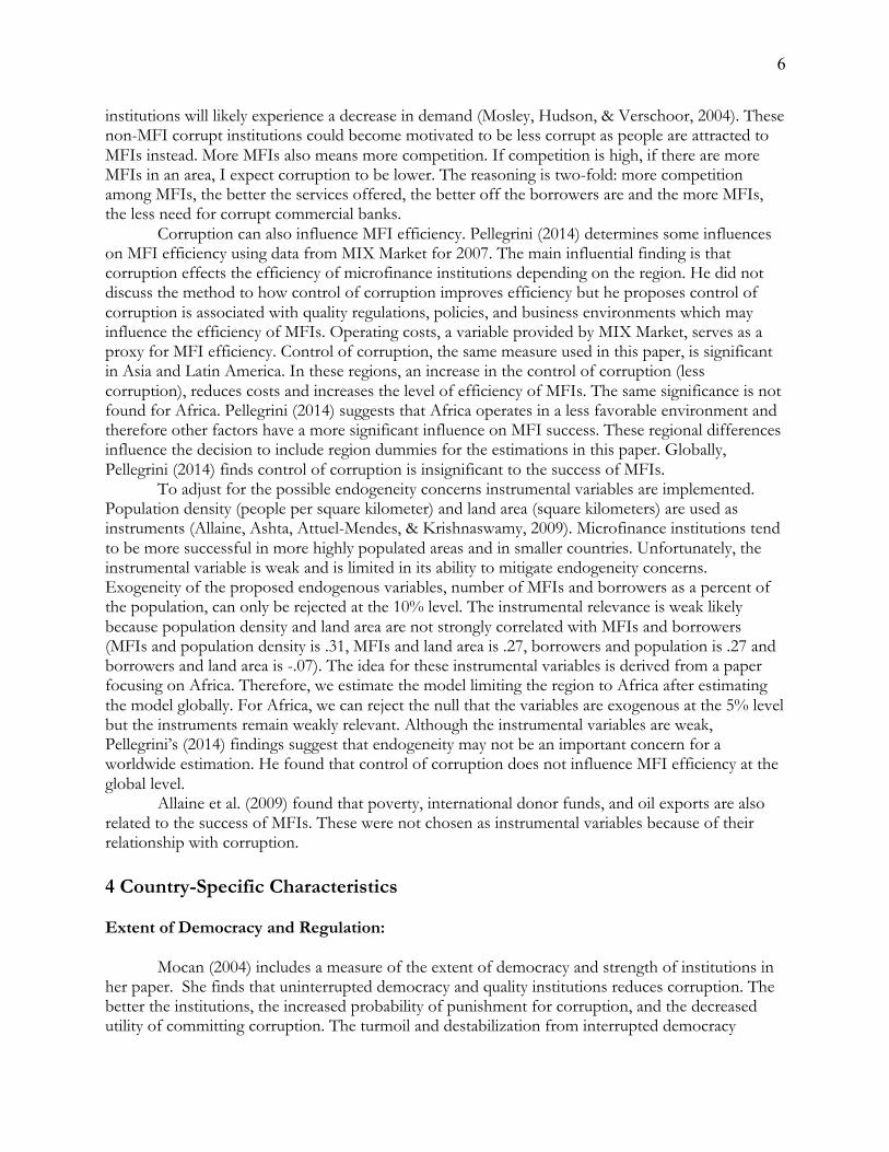
Figures for mean number of borrowers, gross loan portfolio, and MFIs are below. Bangladesh, where microfinance began, reaches the highest number of borrowers relative to the population. Figure 9: Mean borrowers (% population ages 15-64), by country 2000-2015. Source: MIX Market
Country:Bangladesh
19.58%
Country:Zimbabwe
0.12%
0.00 19.58
Borrowers(%ofPop.)
10
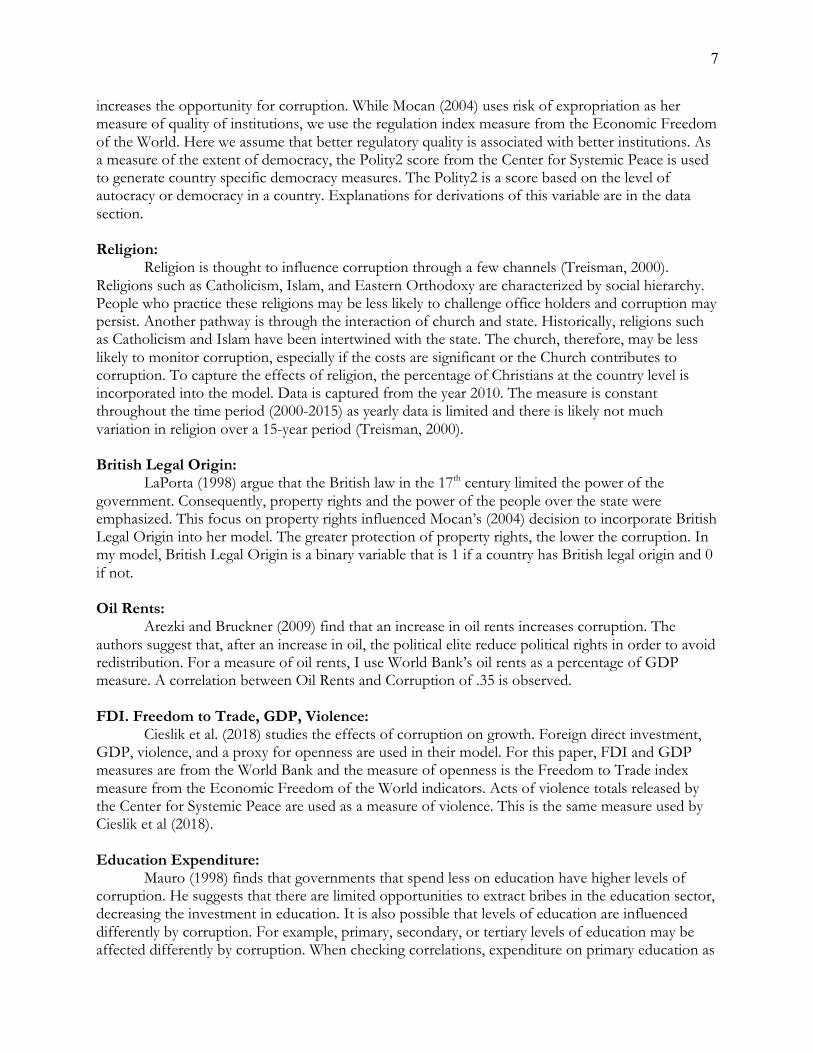
Figure 10: Mean gross loan portfolio, by country 2000-2015 Source: MIX Market
Figure 11: Mean MFIs, by country from 2000-2015 Source: MIX Market
To capture corruption, I use data from the Worldwide Governance Indicators project, referred to as WGI hereafter. WGI provides a control of corruption variable that is used as the dependent variable. Data on macroeconomic indicators (GDP per capita, foreign direct investment net out), financial indicators (domestic credit provided by the financial sector as percent of GDP), and cultural indicators (government expenditure on education as percent of GDP, oil rents as percent of GDP) are from the World Bank. Religious data was collected from the Pew Research Center. A variable describing the extent of democracy was generated from the Polity Project of the Center for Systemic Peace. Legal origin of countries data is from the paper “The Quality of Government” (Shleifer, 2013).
Country:Zimbabwe
GLP:6million
Country:China,People's
Republicof
GLP:6Billion
0 6B
GrossLoanPortfolio
Country:India
MFIs:84
1.00 83.50
MFIs

11
Worldwide Governance Indicators: The WGI project reports indicators for over 200 countries on six dimensions of governance: voice and accountability, political stability and absence of violence/terrorism, government effectiveness, regulatory quality, rule of law, and control of corruption (World Bank, 2018). The reported indicators are based on over 30 data sources (World Bank, 2018). The aggregate indicators are then reported in two ways. The first way is in standard normal units ranging from -2.5 to 2.5 and the second way is in percentile rank terms from 0 to 100 (World Bank, 2018). The higher the value, the better the outcome. The World Bank suggests that year-to-year periods are difficult to interpret which is why 5 year moving averages are calculated for the years 2000 to 2015 (World Bank, 2018). This leaves data for the years 2002-2013. For easier interpretation Al-Azzam’s (2016) method is used to convert control of corruption estimates to a 100-point scale with higher numbers meaning less control of corruption. To transform into a scale of 100, we add 2.5 to the original estimate, multiply by 20, and subtract that number from 100. For example, in 2004, the WGI control of corruption estimate is -1.4. The conversion to a 100-point index is as follows:
100-(-1.4+2.5)20=78 WGI states their measure of control of corruption “captures perceptions of the extent to
which public power is exercised for private gain (The World Bank Group, 2018).” This is similar to the definition provided in the introduction. Data sources for their measure ask questions such as “How common is it for firms to have to pay irregular additional payments to get things done?” and other data sources provide information on frequency of household bribery and corruption amongst public officials (The World Bank Group, 2018).
Corruption is intuitively difficult to measure as there are varied definitions and it typically is not reported or committed in the open. Since direct corruption is difficult to measure, perception of corruption is often used. Mocan (2004) shows that actual corruption and perception of corruption are often different. Throughout the paper we assume that corruption and perception of corruption are the same but the reader should note that this is not likely realistic. While perceptions of corruption are not the most ideal measure, the WGI project uses information from many sources and incorporates the experiences of citizens, entrepreneurs, and experts in the public, private and NGO sectors. This approach may achieve a measure of corruption perception more aligned with actual corruption.
Figures below demonstrate what corruption looks like globally for our data. We observe that the United States has the lowest average corruption score of 19 and Afghanistan has the highest average corruption score of 80. Countries and their corresponding average corruption score can be found in the Appendix 3, Table 5.

12
Figure 12: Mean corruption score, by country 2000-2015 Source: World Bank
Economic Freedom of the World Indicators:
The Economic Freedom of the World index provided measures on freedom to trade internationally and regulation. A higher score, from 0 to 10, means that a country ranks well in that category. For example, a score of 8, Fiji, in regulation means that the regulatory quality in that country is better than the regulatory quality of a country with a score of 7, Uganda. The magnitude of the difference is difficult to interpret. Credit market regulations, labor market regulations, and business regulations are used to calculate the index for regulation. Tariffs, quotas, hidden administrative restraints, controls on exchange rates and controls on the movement of capital are used to determine the level of freedom to trade internationally (Fraser Institute, n.d.).
Major Episodes of Political Violence-Systemic Peace Polity: Violence data were gathered from the Center for Systemic Peace. The dataset accounts for information on international violence, international war, civil violence, civil war, ethnic violence, and ethnic war. The original dataset recognizes that it is difficult to distinguish between civil and ethnic violence because of the overlap in political and social identity attributes. To avoid any confusion, the total acts of violence are used which is the sum of international violence, international, civil violence, civil warfare, ethnic violence, and ethnic warfare (Marshall, 2017). Mocan (2004) finds that uninterrupted democracy influences the corruption a country experiences. For a measure of democracy, we use Polity2 from The Center for Systemic Peace (Marshall, Gurr, & Jaggers, 2017). The Polity2 score measures the degree of democracy or autocracy in a country from a score of -10 to +10 (Marshall M. G., 2017). A score of +10 is strongly democratic and a score of -10 is strongly autocratic. The average Polity2 score for the past 50 years (1965-2015) is generated for each country. This reveals the extent of democracy or autocracy a country has experienced. 6 Model
We are trying to determine the influence of microfinance institutions on corruption using borrowers as a percent of population ages 15-64, number of MFIs, and gross loan portfolio. Our baseline model is the following:
Country:
Afghanistan
80
Country:United
States
19
19.12 79.94
CorruptionScore

13
𝐶𝑜𝑟𝑟𝑢𝑝𝑡𝑖𝑜𝑛)* = 𝐵- + 𝐵/ ln 𝐺𝑟𝑜𝑠𝑠𝐿𝑜𝑎𝑛𝑃𝑜𝑟𝑡𝑓𝑜𝑙𝑖𝑜 )* + 𝐵3Borrowers)* + 𝐵IMFIs)*
+ 𝐵M ln GDPpercapita )* + 𝐵VViolence)* + 𝐵XPolity2)* + 𝐵[Regulation)*+ 𝐵_FreedomtoTrade)* + 𝐵cChristians)* + 𝐵/-BritishLegalOrigin)* + 𝐵//OilRents)* + 𝐵/3FDINetOut)*+ 𝐵/IGovernmentExpenditureonEducation)*+ 𝐵/MDomesticCreditProvidedbytheFinancialSector)*
While this may seem like too many regressors, theory suggests these controls should be
included in the model. By not including these controls, the influence of MFIs could be overestimated. Oil Rents, FDI Net Out, Government Expenditure on Education, and Domestic Credit Provided by the Financial Sector are all provided as a percentage of GDP.
The reader should note that there are missing factors from this model. Cieslik et al. (2018) uses a measure of political stability and Mocan (2004) uses a measurement for the size of government. The author feels that the measure of violence captures enough of the effect of political stability and that regulatory quality combined with the freedom to trade captures enough of the effects of size of government.
Alternate measures of MFI outreach could have been used as well. MIX Market provides a breadth of data. Some measures could have been profit margin or assets.
Robust and median estimations are incorporated because of heteroskedastic concerns and outliers. Testing for heteroskedastic errors shows we can reject the null that the estimates are homoskedastic. This could be driven by errors being correlated with the measures of MFIs. The results of a scatter plot of the predicted value of our dependent variable and the square of the residuals highlight the concerns (Figure 13, Appendix 4). Outlier concerns have been addressed previously in this paper.
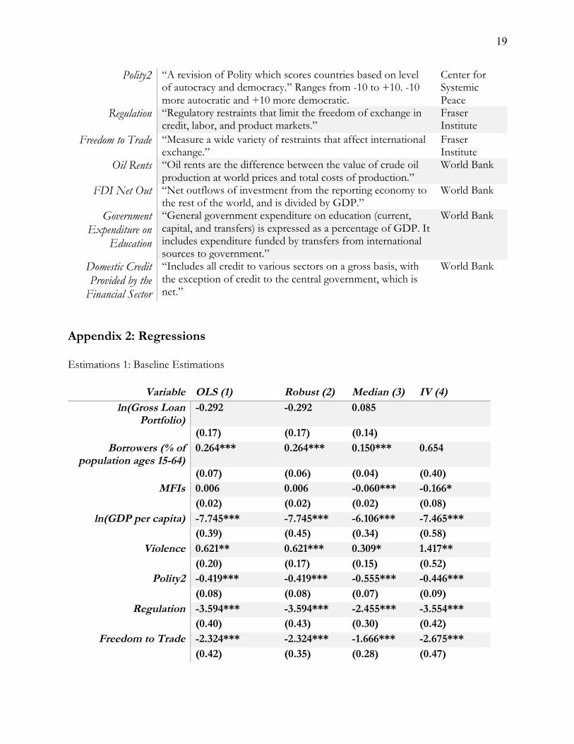
To determine consistency in the model, outliers in gross loan portfolio, number of MFIs, and number of borrowers are excluded in robustness checks. To check for differences across regions, the baseline model is applied to each region. Institutional differences, such as regulation and openness, vary across regions. These differences are addressed in robustness checks. Instrumental variables are implemented to address endogeneity concerns. 7 Results Tables for regressions are included in the Appendix 2. In the following section, when referring to number of borrowers we mean number of borrowers as a percentage of the population ages 15 to 64. All estimates included region and year dummies to control for year and dummy effects. LnGLP refers to the natural log of the gross loan portfolio.
We report data at the country-year level which leaves us with 914 observations. Results include data from 104 distinct countries. The original data on MFIs includes 122 countries but after merging data with WGI, 104 remained. For these countries and over this time period, the median gross loan portfolio is $103 million, the median number of MFIs is 8, the median number of borrowers is 1.6%, and the median corruption score is 62. Of the 104 countries, 34 are in Africa, 20 in Asia, 20 in ECA, 24 in LAC, and 6 in MENA.
The baseline model (1) shows significance of borrowers but no significance of gross loan portfolio or MFIs. The controls all show significance and have the expected sign on their coefficients. For example, the coefficient on violence is positive, suggesting that as violence increases, so does corruption. This makes sense intuitively. The positive coefficient on borrowers (.264) suggests that as borrowers increase, there is more corruption. This is surprising. The theory

14
presented previously in this paper suggests that more borrowers would lead to lower corruption. While the number of borrowers is significant, the coefficient is small (.264). This means that a one-unit increase corresponds to a .264 increase in corruption. Over the time period studied, for all countries, the mean number of borrowers increased 2 percentage points, from 2% to 4%. The robust estimation (2) has similar results to model 1 while median estimation (3) shows different results. In model 3, MFIs and borrowers are significant but LnGLP is not. This is likely being driven by outliers in the data. The sign of the coefficient (-.06) on MFIs matches the original theory; the more MFIs, the less corruption. Number of borrowers remains positive but the coefficient is smaller than the coefficients in model 1 and 2. Mean number of MFIs across all countries increased from 10 to 12 in this time period. This corresponds to a .12 decrease in corruption. The model (4) for the instrumental variable estimation is different from models 1,2, and 3. LnGLP is removed because it does not show significance in the previous models and we use only two instrumental variables. We need at least as many instrumental variables as endogenous variables and so one MFI characteristic had to be removed. Additionally, but not reported, when estimating results using instrumental variables and LnGLP, the instrumental variables remain weak. The instrumental variable estimation (4) shows MFIs as significant but borrowers as insignificant. The coefficient on MFIs is -.166. This has remained consistent throughout the various estimations, continuing the idea that more MFIs has a negative effect on corruption (lowers corruption). Tests for endogeneity show that we can reject the null that the instruments are exogenous at the 10% level for the Durbin and Wu-Hausman test. Although it may not be necessary to include the instrumental variable estimates because they may not be endogenous as previous research suggests (Pellegrini, 2014), it could be useful to observe the results. First-stage results show small R2
statistics for Shea’s partial R-squared. MFIs have a R2 of .06 and borrowers a R2 of .03. This suggests the instruments are weak. The minimum eigenvalue statistic is 11.9 which is larger than 7.0, the 2SLS size of the nominal 5% Wald Test at the 10% level. The reader should note that the F-test for the residuals could not reject the null that the coefficient is 0. This means the errors are heteroscedastic and potentially make results unreliable. When comparing the OLS (1) and instrumental variable model (4), we see that borrowers is insignificant and MFIs is significant in the instrumental variable model. The coefficient sign on borrowers remains the same but the coefficient on MFI changes to -.166. This could be because in the standard OLS model, the reverse causality of corruption and microfinance is not accounted for.
Even if we assume MFIs do lower corruption, these results are not very influential. Over the time period measured, mean MFIs for all countries increased from 10 to 12. According to the instrumental regression (4), corruption would decrease by .33, not even a point and likely not noticeable. These estimations (OLS, Robust, Median, and IV) have mixed results. In models 1,2, and 3, Borrowers is significant while in models 3 and 4, MFIs is significant. In model 3, both are significant. The relatively small coefficients suggest the influence is minimal. Of most interest is the sign of the coefficients which is positive for Borrowers and negative for MFIs. This will be discussed in more detail in the discussion section.
7 Robustness Checks This section will help us determine the robustness of the OLS model. We drop outlier countries for LnGLP, MFIs, and Borrowers. We then run the model controlling for different levels of corruption, democracy, regulation, and for different regions.

15
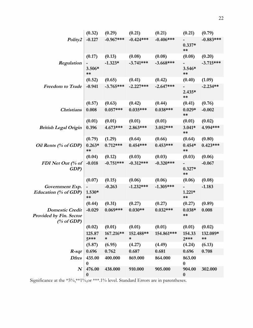
We consider low corruption countries to be those with a corruption score below 50. Countries with medium corruption have a score from 50 up to 70 and low corruption countries have scores above 70. The divisions were based on percentiles. Scores up to 50 include the 25 percentile, 50 to 70 includes the 25-75 percentile, and so forth. For low corruption countries (5), borrowers and MFIs are significant. The coefficient is -.671 for Borrowers and .341 for MFIs. The sign on the coefficients are reversed from model 1. For medium corruption estimates (6), Borrowers is significant and MFIs is not. The coefficient is .147. For high levels of corruption (7), neither MFIs or Borrowers are significant. LnGLP remains insignificant throughout. The switch from significant in the low and medium corrupt countries to insignificant in the high corruption countries could be attributed to other factors contributing to corruption in highly corrupt areas that are too massive to be influenced by microfinance, even minimally. Contrarily, in less corrupt areas, with better regulatory quality for example, microfinance institutions may be able to make more of an impact. China, Peru, Indonesia, and Colombia have the largest gross loan portfolios. All three have mean gross loan portfolio’s above 3 billion. This is in the 95 percentile for gross loan portfolio. After running model 1 again but excluding these countries, gross loan portfolio becomes significant. Similar to model 1, number of borrowers is significant while MFIs are not. The coefficient on gross loan portfolio is -.553. A 1% increase in gross loan portfolio is associated with a .00553 decrease in corruption. This coincides with the original theory. We then estimate OLS models depending on the level of autocracy (9) and democracy (10) a country experiences. Democracies have lower levels of corruption. In our sample, for example, the average corruption score for more democratic countries (those with a Polity2 score above 0) is 56 while the average level of corruption for more autocratic countries is 66 (those with a Polity2 score below 0). We find that for autocracies, MFIs, LnGLP, and Borrowers are insignificant. For democracies, LnGLP and MFIs are significant. This finding is consistent with the idea that autocracies, with higher corruption levels, have other more influential factors contributing to corruption that is difficult to overcome with MFIs. It is interesting that for democracies, the sign on MFIs becomes +.8. This is in opposition to previous results. Outliers in regulatory quality may be affecting our estimations. Fiji, with the highest mean regulation score of 8.2, is excluded and Zimbabwe, with the lowest mean regulation score of 4.2, is excluded in separate estimations. We observe similar results to the original OLS (1) model. Next, we estimate the original OLS model without India. India, over the time period studied, had an average of 92 MFIs. The next closest average MFIs is 54 from Philippines. After excluding India, LnGLP, Borrowers, and MFIs become significant. The coefficient on LnGLP is -.355, is .177 on Borrowers, and is .081 on MFIs. Finally, we separate regression results based on region. While there is not much difference in corruption level across regions (Africa=64, Asia=62, ECA=60, LAC=56, MENA=58), there could be differences in other measures. We find that for Africa and ECA, results are similar to OLS (1). For Asia, MFI is significant but MFIs only increased by 1 over this period (for countries with data from 2000-2015). For LAC, LnGLP and MFIs are significant. For MENA, borrowers and MFIs are significant. Over the time period, active borrowers increased from 2.4 to 6.4 and MFIs from 11 to 20. The final estimation uses instrumental variables for the region Africa. We estimate Africa because Ahlin et al. (2010), after researching MFIs in Africa, suggest that small countries and high population density influences the success of MFIs. We see that Borrowers is significant and has a coefficient of 3.59. This is relatively larger than model 1 where the coefficient is .264. The Wu-Hausman and Durbin test suggest that we can reject the null at the 5% level that the variables are

16
exogenous. According to the minimum eigenvalue statistic, 3.87, the instruments remain weak. 3.87 is less than 7.03, the value of the 2SLS size of nominal 5% Wald test at the 10% level. 8 Discussion An interesting result are the positive coefficients on Borrowers but negative coefficients on LnGLP and MFIs when we observe significance. The original theory suggests that the coefficients would be negative for all three MFI characteristics. This means that as borrowers increase, there would be less corruption. However, this is not what we find. Perhaps with more borrowers, more people have the income to participate in corruption. Microfinance institutions, separate from their services, may lower corruption by their presence. The institutions may pull people away from corrupt financial institutions but loans may allow them to participate in other types of corruption such as bribery. We may also observe MFIs to lower corruption because of competition. The more MFIs, the greater the competition, and the less corruption. Overall, the effects are small, as the coefficients are relatively small. The coefficient on Borrowers in model 1 is .264. Using a corruption score from 0 to 100, this effect is minimal. The mean number of borrowers reached, over the time period studied, increased from 2% to 4% of the population. This would be associated with a .5 increase in corruption (.264*2), which would not be noticed. Another critical observation is the possible reverse causality. Microfinance institutions may be attracted to areas with high corruption. While we attempted to use an instrumental variable, the variables are limited in their effectiveness to mitigate concerns about endogeneity. Assuming that MFIs are more likely to operate in more corrupt areas because of the need, this would bias our results upwards, overestimating the influence of microfinance characteristics. Regional differences are interesting as well. In Africa, a region with a less favorable environment for MFIs, an increase in borrowers has a larger effect on corruption than the effect seen at the global level. Perhaps, MFIs in this area are corrupt, mirroring the environment. Asia, which experiences more efficiency in MFI operations, is positively influenced by MFIs. It is interesting that according to Pellegrini (2014), control of corruption is only significant in Asia and LAC. According to the estimations, these countries experience lower corruption with more MFIs. Reverse causality may be biasing results upward in these areas. LAC and Asia also have the largest gross loan portfolio and larger gross loan portfolios are associated with a decrease in cost due to economies of scale. MFIs in these areas may be better performing and less corrupt, impacting the area more than MFIs in less favorable environments.
An interesting idea relates to Dechenaux et al’s (2014) findings. They find that the frequency of bribery is influenced by MFIs but not the magnitude. With MFIs present, the frequency of bribery may go down so areas with more MFIs have less perceived corruption. Borrowers, instead, are associated with an increase in corruption because the magnitude of bribery remains the same and therefore perceptions remain the same or are worse because people can be asked for larger bribes.
Overall, results vary and are inconclusive. In most regressions where we observe significant of Borrowers, the effect on corruption is to increase corruption. In results where LnGLP is significant, the coefficient is negative, suggesting LnGLP reduces corruption. The sign of the coefficient on MFIs varies depending on corruption level, outliers, and the region. 9 Conclusion This paper has reviewed and assessed the interaction of microfinance institutions and corruption. We find that the effects are minimal and inconsistent across various models and
17
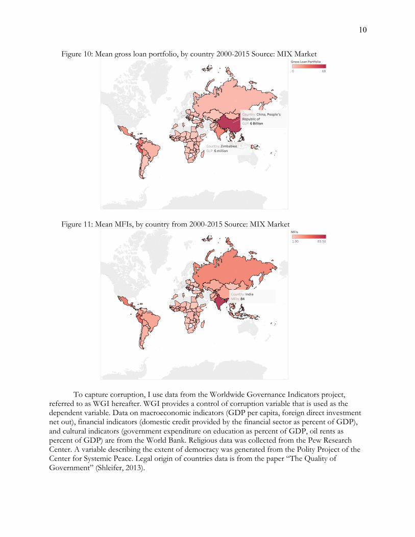
depending on the MFI characteristic, corruption can decrease or increase. More borrowers are associated with an increase in corruption while more MFIs are associated with less corruption, depending on regional effects, levels of corruption, and outliers.
It could be of interest to see what the effects would be if MFIs and borrowers were calculated as a percentage of the poor population instead of the population as a whole, especially since MFIs typically target lower-income populations. It would be also useful to have a stronger instrumental variable. Interaction effects are also not addressed in this paper. For example, GDP and violence could be related in such a way that countries with high and low GDP per capita do not experience as much violence as countries with medium levels of GDP per capita.
A possible next step is to focus research on the relationship between MFIs and corruption on a particular region. Global effects are difficult to determine due to variation in the economic, political, and culture environments across regions.

18
Appendix 1: Definitions Term Definition Source Bank “A licensed financial intermediary regulated by a state
banking supervisory agency. Provides any of a number of financial services, including: deposit taking, lending, payment services, and money transfers.”
MIX Market
Cooperative/Credit Union
“A non-profit, member-based financial intermediary. Offers a range of financial services, including lending and deposit taking, for the benefit of its members. Not regulated by a state banking supervisory agency.”
MIX Market
NGO “An organization registered as a non-profit for tax purposes or some other legal charter. Its financial services are usually more restricted, usually not including deposit taking. These institutions are typically not regulated by a banking supervisory agency.”
MIX Market
Non-bank Financial
Institution
“An institution that provides similar services to those of a Bank, but is licensed under a separate category. The separate license may be due to lower capital requirements, to limitations on financial service offerings, or to supervision under a different state agency.”
MIX Market
Rural Bank “Banking institution that targets clients who live and work in non-urban areas and who are generally involved in agricultural-related activities.”
MIX Market
Control of Corruption
“Captures perceptions of the extent to which public power is exercised for private gain, including both petty and grand forms of corruption, as well as "capture" of the state by elites and private interests.”
WGI
Gross Loan Portfolio
“All outstanding principals due for all outstanding client loans. This includes current, delinquent, and renegotiated loans, but not loans that have been written off. It also includes off balance sheet portfolio.”
MIX Market
Number of active borrowers
“The number of individuals or entities who currently have an outstanding loan balance or are primarily responsible for repaying any portion of the gross loan portfolio. Individuals who have multiple loans are counted as a single borrower.”
MIX Market
Scale “Large: Africa, Asia, ECA, MENA: > 8 million GLP; LAC > 15 million GLP Medium: Africa, Asia, ECA, MENA: 2 million - 8 million GLP; LAC: 4 million - 15 million GLP Small: Africa, Asia, ECA, MENA: < 2 million GLP; LAC: < 4 million GLP”
MIX Market
GDP per capita “Gross domestic product divided by midyear population.” World Bank Violence “Total summed magnitudes of all (societal and interstate)
Major Episodes of Political Violence.” Center for Systemic Peace
19
Polity2 “A revision of Polity which scores countries based on level of autocracy and democracy.” Ranges from -10 to +10. -10 more autocratic and +10 more democratic.
Center for Systemic Peace
Regulation “Regulatory restraints that limit the freedom of exchange in credit, labor, and product markets.”
Fraser Institute
Freedom to Trade “Measure a wide variety of restraints that affect international exchange.”
Fraser Institute
Oil Rents “Oil rents are the difference between the value of crude oil production at world prices and total costs of production.”
World Bank
FDI Net Out “Net outflows of investment from the reporting economy to the rest of the world, and is divided by GDP.”
World Bank
Government Expenditure on
Education
“General government expenditure on education (current, capital, and transfers) is expressed as a percentage of GDP. It includes expenditure funded by transfers from international sources to government.”
World Bank
Domestic Credit Provided by the
Financial Sector
“Includes all credit to various sectors on a gross basis, with the exception of credit to the central government, which is net.”
World Bank
Appendix 2: Regressions Estimations 1: Baseline Estimations
Variable OLS (1) Robust (2) Median (3) IV (4) ln(Gross Loan
Portfolio) -0.292 -0.292 0.085
(0.17) (0.17) (0.14) Borrowers (% of
population ages 15-64) 0.264*** 0.264*** 0.150*** 0.654
(0.07) (0.06) (0.04) (0.40) MFIs 0.006 0.006 -0.060*** -0.166*
(0.02) (0.02) (0.02) (0.08) ln(GDP per capita) -7.745*** -7.745*** -6.106*** -7.465***
(0.39) (0.45) (0.34) (0.58) Violence 0.621** 0.621*** 0.309* 1.417**
(0.20) (0.17) (0.15) (0.52) Polity2 -0.419*** -0.419*** -0.555*** -0.446***
(0.08) (0.08) (0.07) (0.09) Regulation -3.594*** -3.594*** -2.455*** -3.554***
(0.40) (0.43) (0.30) (0.42) Freedom to Trade -2.324*** -2.324*** -1.666*** -2.675***
(0.42) (0.35) (0.28) (0.47)

20
Christians 0.036*** 0.036*** 0.013* 0.042*** (0.01) (0.01) (0.01) (0.01)
British Legal Origin 2.847*** 2.847*** 2.081** 2.496*** (0.64) (0.67) (0.70) (0.72)
Oil Rents (% of GDP) 0.459*** 0.459*** 0.421*** 0.451*** (0.03) (0.03) (0.02) (0.04)
FDI Net Out (% of GDP)
-0.321*** -0.321*** -0.277*** -0.284***
(0.06) (0.05) (0.06) (0.06) Government Exp.
Education (% of GDP) -1.252*** -1.252*** -0.879*** -1.223***
(0.27) (0.27) (0.23) (0.29) Domestic Credit
Provided by Fin. Sector (% of GDP)
0.033*** 0.033*** 0.003 0.033**
(0.01) (0.01) (0.01) (0.01) Constant 152.460*** 152.460*** 125.281*** 154.249***
(4.27) (5.35) (3.90) (4.69) R-squared 0.687 0.687 0.657
Dfres 873.000 873.000 873.000 N 914.000 914.000 914.000 914.000
Significance at the *5%,**1%,or ***.1% level. Standard Errors are in parentheses. Estimations 2: Robustness Checks
LowCorrupt (5)
MedCorrupt (6)
HighCorrupt (7)
GLPOutliers (8)
ln(Gross Loan Portfolio)
-0.546 -0.157 0.056 -0.553**
(0.30) (0.15) (0.23) (0.19) Borrowers (% of
population ages 15-64) -0.671** 0.147** 0.095 0.333***
(0.23) (0.06) (0.08) (0.08) MFIs 0.341** -0.019 -0.010 -0.006
(0.12) (0.02) (0.03) (0.02) ln(GDP per capita) -11.922*** -4.523*** -0.856* -8.185***
(2.00) (0.36) (0.43) (0.40) Violence -6.760*** 0.189 0.680*** 0.906***
(1.97) (0.19) (0.17) (0.22) Polity2 1.184*** -0.253*** -0.321** -0.450***
(0.28) (0.07) (0.11) (0.08) Regulation -5.710*** -1.907*** -2.072*** -3.474***
(1.20) (0.36) (0.43) (0.41)

21
Freedom to Trade -7.913*** -0.981* -0.753* -2.538*** (1.94) (0.39) (0.37) (0.43)
Christians -0.050 0.025*** 0.029* 0.040*** (0.04) (0.01) (0.01) (0.01)
British Legal Origin 14.516*** 1.161* 0.585 3.218*** (3.67) (0.55) (0.78) (0.65)
Oil Rents (% of GDP) -0.054 0.428*** 0.078** 0.463*** (0.98) (0.06) (0.03) (0.04)
FDI Net Out (% of GDP)
0.146 -0.122* -0.026 -0.357***
(0.09) (0.05) (0.05) (0.06) Government Exp.
Education (% of GDP) -1.754 -1.027*** 0.306 -1.112***
(0.98) (0.21) (0.32) (0.28) Domestic Credit
Provided by Fin. Sector (% of GDP)
0.093*** 0.030*** -0.018 0.043***
(0.02) (0.01) (0.02) (0.01) Constant 225.111*** 110.117*** 87.199*** 158.953***
(20.52) (4.02) (3.91) (4.57) R-squared 0.963 0.421 0.671 0.698
Dfres 87.000 568.000 145.000 833.000 N 123.000 608.000 183.000 874.000
Significance at the *5%,**1%,or ***.1% level. Standard Errors are in parentheses. Estimations 3: Robustness Checks Continued
Autoc (9)
Democ (10)
Fiji (11)
Zimbabwe(12)
India (13)
IVAfrica (14)
ln(Gross Loan Portfolio)
0.063 -1.127*** -0.265 -0.285 -0.355*
(0.26) (0.24) (0.17) (0.17) (0.17) Borrowers (% of
population ages 15-64) 0.200 0.146 0.260*** 0.268*** 0.177* 3.590***
(0.15) (0.09) (0.07) (0.07) (0.07) (1.07) MFIs -0.005 0.084** 0.006 0.005 0.081*
* -0.531
(0.05) (0.03) (0.02) (0.02) (0.03) (0.33) ln(GDP per capita) -
4.517***
-9.987*** -7.756*** -7.710*** -7.919***
-4.399***
(0.60) (0.60) (0.39) (0.39) (0.38) (0.93) Violence 2.209*
** 0.087 0.645** 0.581** 0.788*
** 2.903***
22
(0.32) (0.29) (0.21) (0.21) (0.21) (0.79) Polity2 -0.127 -0.967*** -0.424*** -0.406*** -
0.337***
-0.883***
(0.17) (0.13) (0.08) (0.08) (0.08) (0.20) Regulation -
3.506***
-1.323* -3.741*** -3.668*** -3.546***
-3.715***
(0.52) (0.65) (0.41) (0.42) (0.40) (1.09) Freedom to Trade -0.941 -3.765*** -2.227*** -2.647*** -
2.435***
-2.234**
(0.57) (0.63) (0.42) (0.44) (0.41) (0.76) Christians 0.008 0.057*** 0.035*** 0.038*** 0.029*
** -0.002
(0.01) (0.01) (0.01) (0.01) (0.01) (0.02) British Legal Origin 0.396 4.673*** 2.863*** 3.052*** 3.041*
** 4.994***
(0.79) (1.29) (0.64) (0.66) (0.64) (0.80) Oil Rents (% of GDP) 0.263*
** 0.712*** 0.454*** 0.453*** 0.454*
** 0.423***
(0.04) (0.12) (0.03) (0.03) (0.03) (0.06) FDI Net Out (% of
GDP) -0.018 -0.751*** -0.312*** -0.320*** -
0.327***
-0.067
(0.07) (0.15) (0.06) (0.06) (0.06) (0.08) Government Exp.
Education (% of GDP) -1.530***
-0.263 -1.232*** -1.305*** -1.221***
-1.183
(0.44) (0.31) (0.27) (0.27) (0.27) (0.89) Domestic Credit
Provided by Fin. Sector (% of GDP)
-0.029 0.069*** 0.030** 0.032*** 0.038***
0.008
(0.02) (0.01) (0.01) (0.01) (0.01) (0.02) 125.87
5*** 167.216***
152.488***
154.861*** 154.332***
132.089***
(5.87) (6.95) (4.27) (4.49) (4.24) (6.13) R-sqr 0.696 0.762 0.687 0.681 0.696 0.708 Dfres 435.00
0 400.000 869.000 864.000 863.00
0
N 476.000
438.000 910.000 905.000 904.000
302.000
Significance at the *5%,**1%,or ***.1% level. Standard Errors are in parentheses.

23
Estimations 4: Estimations by Region Africa (15) Asia (16) ECA (17) LAC (18) MENA (19)
ln(Gross Loan Portfolio)
-0.407 -0.437 0.093 -1.692** 1.102
(0.28) (0.39) (0.32) (0.52) (0.60) Borrowers (% of
population ages 15-64) 1.767*** 0.046 0.381*** 0.026 -0.827**
(0.36) (0.13) (0.11) (0.14) (0.26) MFIs -0.110 -0.177*** 0.103 0.095* -0.906***
(0.06) (0.05) (0.07) (0.04) (0.20) ln(GDP per capita) -4.485*** -9.658*** -8.851*** -6.551*** -4.427*
(0.60) (1.41) (0.73) (0.72) (1.95) Violence 2.024*** -0.596 3.193* 1.421** 0.242
(0.41) (0.35) (1.47) (0.45) (0.70) Polity2 -1.037*** 1.283*** -0.964*** -1.080*** -3.869***
(0.16) (0.32) (0.19) (0.15) (0.67) Regulation -4.061*** -4.493* -6.839*** 0.666 -3.039*
(0.52) (2.01) (0.82) (0.96) (1.28) Freedom to Trade -2.229*** -7.572*** -4.579*** -4.063*** -0.624
(0.65) (2.15) (0.60) (0.91) (1.26) Christians -0.015 0.041 0.088*** 0.553*** 1.526***
(0.01) (0.02) (0.02) (0.07) (0.18) British Legal Origin 4.931*** -10.168*** 0.000 12.057*** 0.000
(0.76) (2.45) (.) (2.16) (.) Oil Rents (% of GDP) 0.400*** 0.358 0.386*** 0.566*** 0.204*
(0.04) (0.30) (0.07) (0.16) (0.09) FDI Net Out (% of
GDP) -0.163* 1.418 -0.191* -4.601*** 1.284*
(0.07) (0.78) (0.09) (0.57) (0.60) Government Exp.
Education (% of GDP)
-1.709*** 0.783 -1.073** -0.941 1.159***
(0.48) (1.04) (0.32) (0.55) (0.26) Domestic Credit Provided by Fin.
Sector (% of GDP)
0.045** -0.048 0.055** 0.034 -0.115***
(0.02) (0.04) (0.02) (0.02) (0.03) 136.665*** 226.009***
1 98.334*** 119.256**
* 72.482***
(6.33) (21.79) (9.41) (13.42) (18.37) R-sqr 0.762 0.860 0.926 0.893 0.999 Dfres 267.000 128.000
1 56.000 176.000 25.000

24
N 302.000 161.000 1
89.000 208.000 54.000
Significance at the *5%,**1%,or ***.1% level. Standard Errors are in parentheses. Appendix 3: Tables
Table 1: Correlations Variable Corruption
Corruption 1.00 Ln(Gross Loan Portfolio) 0.07 Borrowers (% of adult population ages 15-64) 0.09 MFIs 0.11 ln(GDP) -0.40 Violence 0.17 Polity2 -0.38 Regulation -0.29 Freedom to Trade -0.30 Christians (% of population) -0.20 British Legal Origin -0.04 Oil Rents (% of GDP) 0.31 FDI Net Out (% of GDP) -0.03 Government Expenditure Education (% of GDP) -0.23 Domestic Credit Provided by the Financial Sector (% of GDP)
-0.42
Year -0.01
Table 2: Mean characteristics by level of corruption Variable High Corruption
(>=70) Medium Corruption (<70<=50)
Low Corruption (<50)
Number of Countries 27 75 20 Gross Loan Portfolio $350 million $762 million $297 million Borrowers (% of adult population ages 15-64)
3 3.6 1.8
MFIs 13 15 6 GDP per capita $1,474 $3,202 $7,376 Violence 1.1 0.5 0.22 Polity2 -3 1.2 2.7 Regulation 5.7 6.2 7 Freedom to Trade 6 6.8 7.6 Christians (% of population)
41.2 59.5 66.6

25
British Legal Origin 0.25 0.32 0.35 Oil Rents (% of GDP) 11.3 2 0.41 FDI Net Out (% of GDP) 1.4 1.1 1.9 Government Expenditure Education (% of GDP)
3 4.1 5.14
Domestic Credit Provided by the Financial Sector (% of GDP)
20.9 44.6 73
The following countries change corruption level depending on the year: Rwanda, Pakistan, Papua New Guinea, Paraguay, Togo, Kenya, Kazakhstan, Guinea, Tunisia, Burundi, Brazil, Bangladesh, Central Africa Republic, Georgia, South Africa, Ukraine, Turkey, Uganda.
Table 3: Mean characteristics by region Variable Africa Asia ECA LAC MENA Corruption 63.75 61.84 59.61 56.29 57.70 Gross Loan Portfolio $136 million $1.2
billion $319 million
$957 million
$91 million
Borrowers (% of adult population ages 15-64)
1.45 4.17 3.18 4.67 1.58
MFIs 8.55 22.05 9.73 17.62 5.03 GDP per capita 1150.99 1857.20 4499.46 5208.49 5535.75 Violence 0.42 1.79 0.22 0.35 1.11 Polity2 -1.93 0.66 2.36 3.75 -4.06 Regulation 5.94 6.22 6.68 6.07 6.08 Freedom to Trade 6.17 6.51 7.17 7.34 6.69 Christians (% of population)
59.64 27.43 52.95 87.92 6.99
British Legal Origin 0.48 0.60 0.00 0.09 0.06 Oil Rents (% of GDP) 6.90 1.75 3.02 2.15 7.00 FDI Net Out (% of GDP) 1.43 0.62 2.16 0.56 1.00 Government Expenditure Education (% of GDP)
4.07 3.33 4.10 4.44 4.85
Domestic Credit Provided by the Financial Sector (% of GDP)
27.00 54.55 40.57 48.66 93.04

26
Table 4: Summary statistics for all data Source Variable Description Obs Mean Std.
Dev. Min Max
WGI Corruption Corruption converted to a scale of 100 using WGI estimates
916 60.4 11.1 18.5 81.9
MIX Market
ln(Gross Loan Portfolio)
Natural log of Gross Loan Portfolio
1,052 18.3 2.1 11.4 23.4
MIX Market
Borrowers Borrowers as a % of total population ages 15-64
909 3.0 4.0 0.0 23.1
MIX Market
MFIs Number of MFIs in a country
1,059 12.6 14.2 1.0 103
World Bank
ln(GDP per capita)
Natural log of GDP per capita
1,051 7.5 1.1 4.8 10.7
Center for Systemic Peace
Violence Total acts of violence 1,284 0.6 1.5 0.0 8.0
Center for Systemic Peace
Polity2 From -10 to +10, a higher score means more democratic and a lower score means more autocratic
1,432 0.5 4.7 -9.0 10.0
Economic Freedom of the World
Regulation 0-10, A higher number, the better the regulatory quality
863 6.2 0.8 3.9 8.5
Economic Freedom of the World
Freedom to Trade
0-10, A higher number, the better the freedom to trade
863 6.8 0.9 2.5 8.6

27
Table 4: Summary statistics for all data used in estimations Variable Obs Mean Std.
Dev.
Min Max
Corruption 914 60.5 10.9 19.4 81.9
ln(Gross Loan Portfolio) 914 16.4 6.3 0.0 23.4
Borrowers 914 2.8 4.0 0.0 23.1
MFIs 914 12.0 14.9 0.0 103.0
Pew Research Center
Christians Christians as a % of total population
1,435 54.8 39.2 1.0 100.0
LaPort et al. (1999)
British Legal Origin
1 if country is of British legal origin, 0 if not
1,224 0.3 0.5 0.0 1.0
World Bank
Oil Rents Oil rents a % of GDP 830 3.7 8.9 0.0 58.2
World Bank
Foreign Direct Investment
FDI out as a % of GDP 855 1.2 4.4 -3.7 58.3
World Bank
Government Expenditure on Education
Expenditure on education as a % of GDP
367 4.1 1.4 1.2 8.8
World Bank
Domestic Credit Provided by the Financial Sector
Domestic credit provided by the financial sector as a % of GDP
1,013 43.8 35.6 -8.4 221.7
Year Year 1,575 2008 4.4 2000 2015

28
ln(GDP per capita) 914 7.4 1.6 0.0 10.1
Violence 914 0.6 1.4 0.0 7.4
Polity2 914 0.5 4.5 -9.0 10.0
Regulation 914 4.8 2.7 0.0 8.2
Freedom to Trade 914 5.2 3.0 0.0 8.6
Christians 914 54.9 39.7 0.0 100.0
British Legal Origin 914 0.3 0.4 0.0 1.0
Oil Rents 914 2.9 8.1 0.0 58.2
Foreign Direct Investment 914 1.0 -4.2 1.9 58.3
Government Expenditure on
Education
914 1.4 2.1 0.0 8.8
Domestic Credit Provided by
Financial Sector
914 42.1 -35.5 8.4 194.5
Year 914 2009 2.837005 2004 2013
Table 5: Countries and corresponding average corruption score, 2000-2015 Country Corruption
Score >61 Country Corruption Score
<=61 Afghanistan 80 Kosovo 61 Chad 78 Malawi 61 South Sudan 78 Mozambique 61
Zimbabwe 77 Tanzania 61
Iraq 77 China 60 Angola 76 Zambia 59 Sudan 76 Tonga 58 Haiti 75 India 58 Uzbekistan 74 Argentina 58 Tajikistan 74 Madagascar 57 Cambodia 73 El Salvador 57

29
Guinea-Bissau 73 Solomon Islands 57 Burundi 73 Mexico 57 Bangladesh 73 Serbia 57 Nigeria 73 Senegal 57 Azerbaijan 72 Bosnia and Herzegovina 57 Central African Republic
72 Morocco 57
Cameroon 72 Thailand 56 Guinea 72 Swaziland 56 Papua New Guinea 71 Burkina Faso 56 Paraguay 70 Panama 56 Kenya 70 Peru 56 Kazakhstan 70 Sri Lanka 56 Togo 69 Suriname 55 Pakistan 69 Jamaica 55 Gabon 69 Colombia 55 Ukraine 69 Montenegro 55 Sierra Leone 68 Romania 54 Uganda 68 Belize 54 Honduras 67 Bulgaria 53 Lebanon 67 Fiji 53 Dominican Republic 65 Tunisia 53 Indonesia 65 Ghana 52 Nepal 65 Trinidad and Tobago 52 Ecuador 64 Brazil 51 Niger 64 Georgia 50 Liberia 64 Turkey 50 Moldova 64 Malaysia 48 Nicaragua 64 Rwanda 48 Albania 63 Croatia 47 Philippines 63 Samoa 47 Armenia 63 Jordan 46 Ethiopia 63 South Africa 46 Guatemala 63 Vanuatu 45 Gambia, The 63 Namibia 44 Benin 62 Grenada 42 Vietnam 62 Poland 41 Mali 62 Costa Rica 38 Guyana 62 Hungary 38 Bolivia 62 Bhutan 32 Mongolia 62 Israel 31 Uruguay 24

30
Chile 21 United States 19
Appendix 4: Figures Figure 1: Mean corruption score, all countries 2003-2013, using moving averages Source: World Bank
We find that the mean corruption score has not changed significantly over the time period studied.
Figure 2: Mean corruption score, by level of corruption, 2003-2013, using moving averages Source: World Bank
Even by separating by level of corruption, there is not much variation over time.
Figure 3: Mean borrowers, 2003-2013, using moving averages Source: MIX Market
6060.2
60.4
60.6
60.8
Corruption
2000 2005 2010 2015Year
Corruption
4050
6070
80C
orru
ptio
n Sc
ore
2000 2005 2010 2015Year
High Corruption Medium CorruptionLow Corruption
Corruption Score by Level of Corruption

31
Figure 4: Mean MFIs, 2003-2013, using moving averages Source: MIX Market
Around the financial crisis number of MFIs decreases. Figure 5: Mean gross loan portfolio, 2003-2013, using moving averages Source: MIX Market
1.5
22.
53
3.5
4Bo
rrow
ers(
% o
f Pop
ulat
ion)
2000 2005 2010 2015Year
Average Borrowers (% of Population)
810
1214
16M
FIs
2000 2005 2010 2015Year
Average MFIs

32
Figure 6: Corruption and MFIs by country, 2003-2013, using moving averages Source: World Bank and MIX Market
MFIs clustered at the top suggesting MFIs are more likely to be in corrupt areas. Outliers to the right driven by India.
Figure 7: Corruption and borrowers by country, 2003-2013, using moving averages Source: World Bank and MIX Market
020
040
060
080
010
00G
ross
Loa
n Po
rtfol
io (m
illion
s)
2000 2005 2010 2015Year
Average Gross Loan Portfolio
2040
6080
Cor
rupt
ion
0 20 40 60 80 100MFIs
Corruption and MFIs

33
Outliers to the right driven by Bangladesh. Figure 8: Corruption and gross loan portfolio by country, 2003-2013, using moving averages Source: World Bank and MIX Market
Outliers to the right driven by Indonesia. Figure 13: Predicted value of corruption and square of residuals
2040
6080
Cor
rupt
ion
0 5 10 15 20 25Borrowers(% of Population)
Corruption and Borrowers(% of Population)
2040
6080
Cor
rupt
ion
0 500 1000 1500Gross Loan Portfolio(millions)
Corruption and Gross Loan Portfolio

34
020
040
060
080
0s1
s
20 40 60 80Linear prediction

35
References DATA Center for Systemic Peace. (2016). INSCR Data Page. Retrieved from Systemic Peace:
http://www.systemicpeace.org/inscrdata.html Fraser Institute. (2018). Economic Freedom. Retrieved from fraser institute:
https://www.fraserinstitute.org/economic-freedom/dataset MIX Market . (2018). Cross Market Analysis. Retrieved from themix:
https://reports.themix.org/crossmarket Pew Research Center. (2015, April 2). Religious Composition by Country, 2010-2050. Retrieved from Pew
Forum: http://www.pewforum.org/2015/04/02/religious-projection-table/ Shleifer, A. (2013, March 7). The Quality of Government. Retrieved from scholar.harvard.edu:
https://scholar.harvard.edu/shleifer/publications/quality-government World Bank. (2018). World Bank Open Data. Retrieved from worldbank: https://data.worldbank.org/ World Bank. (2018). Worldwide Governance Indicatorrs . Retrieved from World Bank: http://info.worldbank.org/governance/wgi/#home LITERATURE Ahlin, C., Lin, J., & Maio, M. (2010). Where does microfinance flourish? Microfinance
institution performance in macroeconomic context. Journal of Development Economics. Aidt, T. S. (2009). Corruption, institutions, and economic development. Oxford Review of
Economic Policy, 25(2), 271-291. Al-Azzam, M. (2016). CORRUPTION AND MICROCREDIT INTEREST RATES: DOES
REGULATION HELP? Bulletin of Economic Research. Allaine, V., Ashta, A., Attuel-Mendes, L., & Krishnaswamy, K. (2009). Institutional Analysis to
Explain the Success of Moroccan Microfinance Institutions. Cahier du CEREN, 29, 6-26. Arezki , R., & Brückner , M. (2009, December). Oil Rents, Corruption, and State Stability:
Evidence From Panel Data Regressions. IMF. Arnone, M., & Borlini, L. S. (2014). Opening Remarks: corruption and economic analysis. In M.
Arnone, & L. S. Borlini, Corruption: Economic Analysis and International Law (pp. 13-18). Northampton, Massachusetts, USA: Edward Elgar Publishing, Inc. .
Banerjee, A., Karlan, D., Osei, R. D., Trachtman, H., & Udry, C. (2018). UNPACKING A MULTI-FACETED PROGRAM TO BUILD SUSTAINABLE INCOME FOR THE VERY POOR. NATIONAL BUREAU OF ECONOMIC RESEARCH.
Bank, T. W. (1997). The State in a Changing World. New York: Oxford University Press. Basu, K. (2006). GENDER AND SAY:A MODEL OF HOUSEHOLD BEHAVIOUR
WITHENDOGENOUSLY DETERMINED BALANCE OF POWER. The Economic Journal, 558-580.
Center for Systemic Peace. (2016). INSCR Data Page. Retrieved from Systemic Peace: http://www.systemicpeace.org/inscrdata.html
Cepeda, I., Lacalle-Calderon, M., & Torralbe, M. (2017, November 16). Microfinance and Violence Against Women in Rural Guatemala. Journal of Interpersonal Violence, 1-23.
Chaudhuri, S., & Gupta, M. R. (1996). Delayed formal credit, bribing and the informal credit market in agriculture: A theoretical analysis. Journal of Development Economics, 51(2), 433-449.
Cieślik, A., & Goczek, Ł. (2018, March). Control of corruption, international investment, and economic growth – Evidence from panel data. World Development, 323-335.
36
Dalal, K., Dahlstrom, O., & Timpka, T. (2013). Interactions between microfinance programmes and non-economic empowerment of women associated with intimate partner violence in Bangladesh: a cross-sectional study. BMJ Open.
Dechenaux, E., Lowen, A., & Samuel, A. (2014). Bribery in subsidized credit markets: evidence from Bangladesh. Indian Growth and Development Review; Bingley, 7(1), 61-72.
Duflo, E., Banerjee, A., Glennerster, R., & Kinnan, C. G. (2013, May). The Miracle of Microfinance? Evidence from a Randomized Evaluation.
Federal Financial Institutions Examination Council . (2018, February 21). Consolidated Reports of Condition and Income. Retrieved from Federal Reserve: https://www.federalreserve.gov/Releases/chargeoff/delallsa.htm
Field, E., Holland, A., & Pande, R. (2014, September 29). Microfinance: Points of Promise. Journal of Policy Analysis.
Fraser Institute. (2018). Economic Freedom. Retrieved from fraser institute: https://www.fraserinstitute.org/economic-freedom/dataset
Fraser Institute. (n.d.). Approach. Retrieved March 2018, from Fraser Institute: https://www.fraserinstitute.org/economic-freedom/approach
Frey, A. (2017, Juney). CASH TRANSFERS, CLIENTELISM, AND POLITICAL ENFRANCHISEMENT: EVIDENCE FROM BRAZIL∗.
Giridharadas, A., & Bradsher, K. (2006, October 13). Microloan Pioneer and His Bank Win Nobel Peace Prize. Retrieved from The New York Times : https://www.nytimes.com/2006/10/13/business/14nobelcnd.html
IMF. (2016, May). Corruption: Costs and Mitigating Strategies. Retrieved from IMF: https://www.imf.org/external/pubs/ft/sdn/2016/sdn1605.pdf
La Porta, R., Lopez-de-Silanes, F., & Shleifer, A. (1998, December). Law and Finance. Journal of Poltical Economy.
Lui, F. (1985). An Equilibrium Queuing Model of Bribery. Journal of Political Economy, 760-781.
Marshall, M. G. (2017, July 25). MEPVcodebook2016. Retrieved from Systemic Peace: http://www.systemicpeace.org/inscr/MEPVcodebook2016.pdf
Marshall, M. G., Gurr, T. R., & Jaggers, K. (2017, July 25). p4manualv2016. Retrieved from Systemic Peace: http://www.systemicpeace.org/inscr/p4manualv2016.pdf
Mauro, P. (1995, August). Corruption and Growth. The Quarterly Journal of Economics,, 110(3).
MIX Market . (2018). Cross Market Analysis. Retrieved from themix: https://reports.themix.org/crossmarket
MIX Market. (2015). Global Outreach & Financial Performance Benchmark Report - 2015. Retrieved from https://www.themix.org/sites/default/files/publications/global_benchmark_report_fy2015_0.pdf
Mocan, N. (2004, April). WHAT DETERMINES CORRUPTION? INTERNATIONAL EVIDENCE FROM MICRO DATA. NBER.
Mosley, P., Hudson, J., & Verschoor, A. (2004). AID, POVERTY REDUCTION AND THE ‘NEW CONDITIONALITY’. The Economic Journal, 217-243.
Muriu, P. W. (2016). Do Microfinance Profits Converge? Pan-African Evidence. Journal of Economics and Sustainable Development.

37
Pellegrini, C. B. (2014). Operational efficiency, corruption, and political stability in microfinance. In M. Arnone, & L. S. Borlini, Corruption: Economic Analysis and International Law (pp. 129-149). Northampton, MA, USA: Edward Elgar Publishing, Inc.
Pew Research Center. (2015, April 2). Religious Composition by Country, 2010-2050. Retrieved from Pew Forum: http://www.pewforum.org/2015/04/02/religious-projection-table/
Shleifer, A. (2013, March 7). The Quality of Government. Retrieved from scholar.harvard.edu: https://scholar.harvard.edu/shleifer/publications/quality-government
The Economist. (2018, January 27). Bucks after the bang. The World Bank Group. (2018). WGI. Retrieved from worldbank:
http://info.worldbank.org/governance/wgi/#doc The World Bank. (n.d.). SDG Atlas 2017. Retrieved from worldbank:
http://datatopics.worldbank.org/sdgatlas/SDG-01-no-poverty.html Treisman, D. (2000). The causes of corruption: a cross-national study. Journal of Public
Economics, 399-457. Treisman, D. (2003). Postcommunist Corruption. Political Economy of Transition and
Development: Institutions, Politics, and Policies, 201-226. USAID. (2015, May). The Impact of Microcredit Loans on Child Outcomes: A Review of the
Literature. Retrieved from marketlinks: https://www.marketlinks.org/sites/default/files/resource/files/STRIVE_microcreditLitReview-Final2015.pdf
World Bank. (2018). World Bank Open Data. Retrieved from worldbank: https://data.worldbank.org/
World Bank. (2018). Worldwide Governance Indicatorrs . Retrieved from World Bank: http://info.worldbank.org/governance/wgi/#home
World Bank. (2018). Worldwide Governance Indicators . Retrieved from World Bank: http://info.worldbank.org/governance/wgi/#home
Zeller, M. (1999). The Role of Micro-Finance for Income and Consumption Smoothing. Inter-American Development Bank.