UNIVERSITY OF TARTUInstitute of Computer ScienceComputer Science Curriculum

Salijona Dyrmishi

Creating a novel approach for mobilepositioning based on CDR data

Master’s Thesis (30 ECTS)

Supervisor: Amnir Hadachi, PhD.

Tartu 2019-2020

Creating a novel approach for mobile positioning based on CDR data

Abstract:

User geographical positioning is important for many fields that rely on passive geo-location analytics, like targeted marketing, urban and rural transportation planning,public health, etc. A new popular type of data that is commonly used for passive mobilityanalysis is mobile data or the so-called Call Detail Records (CDR). The CDR eventsare stored by mobile operators for the primary purpose of billing. They are generatedevery time we use SMS, call, or internet services. CDR data events are becoming morefrequent due to the lower costs of using mobile services and smartphones becoming anecessary tool in our daily life. However, CDR data has two major drawbacks: temporaland spatial uncertainties. Although the first problem is widely covered by trajectoryreconstruction techniques, the second problem still remains challenging. Hence, in thisthesis, we propose the usage of a new method based on the Sequential Monte Carloalgorithms called particle filtering. The particle filtering application implemented in thisthesis models the trajectory movement to predict the user’s position in a given area. Thismethod uses CDR data and solely the information related to the area of the coveragefrom mobile towers. Our goal is to evaluate if this nonlinear method can out-perform theexistent linear methods like Switching Kalman Filter. Therefore, the model performanceand the effects of the parameters on accuracy were evaluated in controlled experimentalsettings. Additionally, experiments were performed on a dataset from a real case studyand compared with the results achieved by existing methods. Finally, the usability of themethod and future work is discussed.

Keywords: mobile data, particle filtering, location prediction, trajectory prediction

CERCS: P170 (Computer science, numerical analysis, systems, control)

2

Uue lähenemisviisi loomine mobiilse positsioneerimise jaoks CDR-andmete põhjal

Lühikokkuvõte:

Kasutaja geograafiline positsioneerimine on oluline paljudes valdkondades, kus kasu-tatakse inimeste asukohapõhiseid andmeid, näiteks turunduses, linna- ja maatranspordikavadamisel, rahvatervise uurimisel jne. Uut tüüpi andmed, mida kasutatakse passiivseliikuvuse analüüsimisel, on mobiilse andmeside kasutamisel salvestunud kirjed (CDR -Call Data Records). Tavaliselt salvestavad mobiilioperaatorid CDR-sissekandeid arvel-duse eesmärgil. Neid genereeritakse iga kord, kui kasutame SMS-, kõne- või Interneti-teenuseid. Logitud CDR-andmete maht on järjest kasvanud, kuna mobiilsed teenusedon läinud odavamaks ja nutitelefonide kasutamine on muutunud vajalikuks tööriistaksmeie igapäevaelus. CDR-andmetel on siiski kaks suurt puudust: ajaline ja ruumilineebatäpsus. Ehkki esimest probleemi käsitlevad trajektoori rekonstrueerimise tehnikadlaialdaselt, on teine probleem endiselt väljakutsuv. Seetõttu teeme käesolevas lõputöösettepaneku kasutada uut meetodit, mis põhineb järjestikuste Monte Carlo algoritmidel jamida nimetatakse osakeste filtreerimiseks. Selles lõputöös rakendatud osakeste filtreeri-mise rakendus modelleerib trajektoori liikumist, et ennustada kasutaja asukohta antudpiirkonnas. See meetod kasutab CDR-andmeid ja ainult mobiilside tornide levialagaseotud teavet. Meie eesmärk on hinnata, kas see mittelineaarne meetod suudab ületadaolemasolevaid lineaarseid meetodeid nagu näiteks Kalmani filtri kasutamine. Seetõttuhindasime kontrollitud katseseadistustes mudeli jõudlust ja parameetrite mõju täpsusele.Lisaks tehti katseid reaalajas uuringu andmestikuga ja võrreldi olemasolevate meetoditeabil saadud tulemustega. Lõpuks arutasime meetodi kasutatavuse ja edasise töö üle.

Võtmesõnad: mobiilne andmeside, osakeste filtreerimine, asukoha ennustamine, trajek-toori ennustamine

CERCS: P170: Arvutiteadus, arvutusmeetodid, süsteemid, juhtimine (automaatjuhtimis-teooria)

3

Acknowledgement

First, I would like to express my gratitude to my supervisor Dr. Amnir Hadachi forproposing such an interesting topic, always having a positive attitude and for encouragingme to continue further even when I felt like it was not worth it. I would like to thankArtjom Lind for providing the necessary technical help and always being available forsome extra explanations and questions. Additionally, I would like to acknowledge thework of Dr. Amnir Hadachi and Oleg Batrashev on providing a starting point for thecode implementation.

Many thanks to my friends whose physical or virtual presence and support has kept mesane during this intensive period. Additionally, I could not finish the writing processin time without daily encouragement from Sri. Thank you for always believing in myacademic abilities, proofreading this document, and your love. Most importantly I wouldlike to thank my family, my brother Ledio, and my parents Eqerem and Alime, foralways considering my education a priority. I always have felt their genuine interestthrough questions related to my university and work projects. They have supported meunconditionally in every decision and without their sacrifices I would not have achievedthis milestone.

4

Contents

1 Introduction 7

1.1 Problem statement . . . . . . . . . . . . . . . . . . . . . . . . . . . . 7

1.2 Contributions . . . . . . . . . . . . . . . . . . . . . . . . . . . . . . . 8

1.3 Road-map . . . . . . . . . . . . . . . . . . . . . . . . . . . . . . . . . 9

2 Background 10

2.1 Global System for Mobile communication . . . . . . . . . . . . . . . . 10

2.1.1 GSM network components . . . . . . . . . . . . . . . . . . . . 10

2.1.2 GSM cell localization . . . . . . . . . . . . . . . . . . . . . . 12

2.2 Call Detail Records (CDR) . . . . . . . . . . . . . . . . . . . . . . . . 13

2.3 CDR based localization and human mobility analytics: A literature review 14

3 Methodology 17

3.1 Particle filtering . . . . . . . . . . . . . . . . . . . . . . . . . . . . . . 18

3.2 Particle filtering for mobile user localization . . . . . . . . . . . . . . 20

4 Experiments 25

4.1 Evaluation metrics . . . . . . . . . . . . . . . . . . . . . . . . . . . . 26

4.2 Model evaluation in synthetic data . . . . . . . . . . . . . . . . . . . . 27

4.2.1 Dataset description . . . . . . . . . . . . . . . . . . . . . . . . 27

4.2.2 Results . . . . . . . . . . . . . . . . . . . . . . . . . . . . . . 29

4.3 Case study: Real CDR data . . . . . . . . . . . . . . . . . . . . . . . . 32

4.3.1 Dataset description . . . . . . . . . . . . . . . . . . . . . . . . 32

4.3.2 Results . . . . . . . . . . . . . . . . . . . . . . . . . . . . . . 34

5 Discussions 38

5.1 Insights from the implementation and the results of the experiments . . 38

5

5.2 Future work . . . . . . . . . . . . . . . . . . . . . . . . . . . . . . . . 40

6 Summary 41

7 Conclusion 43

References 46

II. Licence . . . . . . . . . . . . . . . . . . . . . . . . . . . . . . . . . . . . 47

6

1 Introduction

Geo-localization as a service is the base of many applications in today’s digital world.Active mobile positioning is important in order to serve customers in a timely mannerbut as well in critical cases like emergency calls. The source of localization data isdifferent mainly to different technologies used (GSM, CDMA). Often the choice of thetechnologies is a trade-off between the costs and the information gain from the data.Today, most of the geo-localization services base their estimations on GPS data whichhas high accuracy especially when the line of sight is clear. Additionally, the sample ratestarting as low as one event per second makes GPS data really dense.

On the other hand, passive mobile positioning gives access to understanding the spatio-temporal behavior of the users. Lately, this type of data is used in a vast pool of fieldslike mining human mobility patterns, urban planning, tourism estimation, vaccinationplanning, public transport rescheduling, etc. The reason for the popularity in so manyfields is mainly because passive mobile positioning serves as a great replacement fortraditional methods that build models upon samples rather than data. The commonpassive mobile positioning data are the logs from Mobile Network Operators (MNO).Every time we use the mobile phone to make a phone call, send an SMS, or use 4G/5Ginternet packages they store what is called Call Detail Records (CDR) for the primarypurpose of billing. Nowadays, there is no doubt that the mobile penetration rate isincreasing even in the most rural/ unreachable places. Additionally, the cost reduction oftelecom services has contributed to a wider geographical spread of the CDR data, as wellas an increase in its frequency. This situation is promising for an increase in importancefor CDR data and probably an expansion to other fields.

1.1 Problem statement

GPS data is highly desirable but it is not the most appropriate choice for passive analysesmainly due to the limitations related to its availability. It is not possible to have GPSrecords for every mobile phone user, simply because many are concerned about privacyand they are not comfortable sharing their location. Additionally, the GPS-enabledreceiver performs complex calculations, and their processing power requirements drainsthe battery of mobile devices really fast. On the contrary, CDR data is easily availableconsidering the fact that the Mobile Network Operators (MNO) always store them andcan be retrieved for all users of a network. This feature makes CDR highly desirable forpassive spatio-temporal analysis, however, they have some disadvantages.

The first disadvantage comes from the fact that the radius of the tower coverage introduces

7

difficulties for the exact user positioning. Every CDR record is coupled with the coveragearea of the tower where the user is connected. These areas, called cells, do not haveunique shapes. They vary from the height of the tower location, the urban environmentaround the tower, population density, the obstacles, etc. The radius of the cell rangesfrom several meters in urban areas to tens of kilometers in rural areas. Within this radius,the location of the mobile phone user is actually unknown. The second disadvantageis related to temporal uncertainties. Being that CDR data is not collected in constantpredefined intervals, the gaps between two consecutive events can be really considerable.They might start from one minute to several hours. Unfortunately, the last one is acommon case. The high level of spatial and temporal uncertainties can have a negativeeffect on the reliability of the studies related to human mobility patterns.

In order to reduce the uncertainties, it is necessary to apply models that will firstly pre-process CDR data like eliminating undesirable effects related to network functionalities.Secondly, it is necessary to reduce temporal uncertainties by building models that willfill in the gaps between consecutive events. Thirdly, estimating the user location withinthe cell in order to reduce spatial uncertainties. From the study of related literature, wehave noticed that the majority of studies apply the first technique before performingaggregated analysis in fields like tourism, healthcare, transport planning, etc. Fewerstudies deal with trajectory reconstruction for the gaps. Lastly, only a couple of studiestries to localize the users within the coverage areas of the towers.

1.2 Contributions

This thesis aims to introduce a new non-linear technique, based on Sequential MonteCarlo Methods named Particle Filtering, to predict the position of the mobile user withina given area. It is in this research’s interest to evaluate if mobile positioning can occurwith decent accuracy using only the minimum required CDR information which includesthe timestamp of the generated event and the coverage area of the tower. The maincontribution of this thesis will be exploring if it is possible by using a nonlinear approachto enhance the mobile positing compared to the existing linear approaches.

We will try to answer this question following the steps as below:

• Propose an application of Particle Filtering to estimate the mobile user positionusing CDR data.

• Systematically evaluate the proposed model in experimental settings and real-worlddata.

8

• Compare the non-linear Particle Filtering method with existing linear methods.

This is a challenging task and not a largely explored area. This work is among the few thatstudy the problem of the user positioning using only the minimum required informationfrom CDR data. Additionally, previous studies consider only linear approaches. Werecognize that human mobility does not follow a linear model, therefore, we are proposingParticle Filtering. Improvements in user positioning will reduce CDR uncertainties andcan bring CDR data closer to GPS data regarding accuracy.

1.3 Road-map

The rest of this thesis is organized as follows:

Chapter 2 (Background): This chapter introduces the user with all the necessarybackground terms, history, and context to understand the source of the problem. Inaddition, it gives an overview of already present mobile data-related research.

Chapter 3 (Methodology): This chapter presents the basic concepts of the particlefiltering as an introduction to the work done for this thesis. Afterward, it demonstratesstep by step the adaption of the particle filter for user positioning based on CDR data.

Chapter 4 (Experiments): This chapter describes the experimental setup and thedatasets used to evaluate the model. It is followed by a short description of the evaluationmetrics. At the end of every experiment done, it displays the outcomes and results in theform of tables and graphs.

Chapter 4: (Discussions) In this chapter we will discuss the outcomes of the experimentand the main lessons we have derived. Based on these discussions a road-map for futurework will be provided.

9

2 Background

This chapter will provide the necessary information for understanding the scope and theterminologies of this project. The first section will describe how the mobile network isfunctioning. It is necessary to understand its components and interaction with mobileterminals in order to understand the challenges and opportunities that arise while usingmobile data for user localization. The second part describes the structure of the logscollected by mobile operators. And lastly, the third section gives an overview of thecurrent research that uses CDR data.

2.1 Global System for Mobile communication

Almost all Mobile Network Operators (MNO) in the world use two main mobile technolo-gies: Global System for Mobiles(GSM) and Code Division Multiple Access (CDMA).GSM technology was first launched in Finland in 1991. It was developed by EuropeanTelecommunications Standards Institute (ETSI) to describe the protocols for 2G mobilecommunications. Presently, GSM comprises approximately 90% of mobile connectionsworldwide, being the most widely used digital mobile telephony system nowadays [1].Therefore, in our study, we will concentrate only on understanding the functionality ofGSM networks.

Definition 1. The global system for mobile communication (GSM) is a globally acceptedstandard for digital cellular communication. GSM is the name of a standardization groupestablished in 1982 to create a common European mobile telephone standard that wouldformulate specifications for a pan-European mobile cellular radio system operating at900 MHz [2].

2.1.1 GSM network components

The GSM network is based on four separate components: the mobile device itself, thebase station subsystem (BSS), the network switching subsystem (NSS), and the supportsubsystem (OSS) [2]. The Subscriber Identity Module (SIM) card is tied to a specificnetwork within GSM network. Every part of the infrastructure of this sub-network makessure to serve to the device where the SIM card is integrated. The functionalities of eachcomponent are described below:

10

• Mobile device

The mobile device connects to the network via hardware. The SIM card providesthe network with identifying information about the mobile user.

• Base station subsystem (BSS)

The BSS handles traffic between the cell phone and the NSS. It consists of two maincomponents: the base transceiver station (BTS) and the base station controller(BSC). The BTS contains the equipment that communicates with the mobilephones, largely the radio transmitter-receivers and antennas, while the BSC, is theintelligence behind it. The BSC communicates with and controls a group of BTSs.

• Network switching subsystem (NSS)

The NSS portion of the GSM network architecture, often called the core network,tracks the location of callers to enable the delivery of cellular services. The NSS isowned by mobile carriers.

• Support subsystem (OSS)

The OSS is the functional entity from which the network operator monitors andcontrols the system. An important function of OSS is to provide a network overviewand support the maintenance activities of different operation and maintenanceorganizations.

The GSM network is made up of geographic areas. As shown in Figure 1, every BTShas a radius of coverage represented by the hexagons. In the MNO terminology, they areidentified as cells. Several cells together are part of a Local Area Connector (LACs).

Definition 2. A cell is the area given radio coverage by one BTS.

The GSM network identifies each cell via a unique assigned number named cell globalidentity (CGI). The cell size can vary from less than 1 km2 to several km2. In areas withdense population, the cell size tends to be smaller compared to rural areas. There are fourdifferent types of cells: pico, micro, macro, and umbrella. The coverage area for eachtype depends on their location environment and the height where they are positioned.Typically, pico cells are used mostly indoor with a radius of 4 - 200 meters. Micro cellsare usually used in urban areas with coverage between 200 m and 2 km. They serve tomalls or other important hubs. Macro cells make about 90% of GSM networks and theirradius varies somewhere from 1 km to 30 km. Umbrella cells cover the gaps betweenseveral micro cells and serve often as a solution for network overloading. In reality, theshape of the cells does not follow the regular hexagon pattern that we illustrated in Figure1. Additionally, there are often overlaps between two cells and sometimes there are gaps.[3][4]

11

Figure 1. Overview of the mobile network

2.1.2 GSM cell localization

At an initial stage when a terminal (mobile device) is switched on, it goes into IDLE mode.When the terminal is in IDLE mode it will connect to the BTS with the strongest signal.Due to noise, this is not necessary the nearest base station. After the initial connectionis established, the connection switches to the Dedicated mode where everything issynchronized and information can be exchanged. When the terminal is in Dedicatedmode the GSM network algorithm decides about handover between cells. The decision isbased on the load of the cells and the motion pattern of the terminal. The goal is to servethe terminal with high quality but as well to equally distribute the load of the BTSs. Dueto this algorithm, the selected cell might not always be the nearest. When the handoverhappens frequently in a couple of seconds, we are dealing with the ping pong effect. Inreality, the user has not moved but due to the ping pong effect, the CDR data reflectsback and forth movements. When moving between different cells, a terminal sends alocation update only when it enters a cell that is not in the previous LAC. [3]

12

2.2 Call Detail Records (CDR)

Today 66.77% of the world’s population has a mobile device, which equals to 5.17 billionpeople. In 2017, the percentage of people owning at least one mobile device was 53%.And by 2023, the prediction is that the number of mobile device users will increaseto 7.33 billion [5]. The percentage is considerably high considering that a part of thepopulation by default can not have a mobile device i.e. underage children or people inremote areas with no access to electricity. With the increasing number of mobile usersand the time we spend using our devices, there is an expected increase on the scale andfrequency of mobile data as well. Mobile data is considered as an interchangeable termwith CDR which are logs generated by the activity of using mobile devices.

Fiadino et al. [6] have taken under study CDR datasets describing the activity ofcustomers from all mobile operators in Spain, from 2014 and 2016. Their comparison ofthe data quality showed that the number of daily data connection has increased in 2016from 10.9 to 50.1 and overall the daily action count grew by 4 times. The data connectioncustomer share had the largest growth from 50% to 85%. Several factors were consideredlike Days of Visibility, Hourly Action Rate, Average Lag Time, Total Inactive Time, andEntropy on this study. The authors revealed that all of them had marked improvementsfrom 2014 to 2016. This study is a good indicator that the user patterns have changedand the CDR data is becoming more fine-grained for mobility studies.

Telecommunication companies store mobile data logs or CDR mainly for billing purposes.The term might be misleading because it dates from the time when the only serviceyou could use were mobile calls but nowadays they are triggered on the event of calls,sending/receiving SMS, and using Internet services. In particular cases, the configurationallows the generation of mobile logs additionally every time the user switches cells orLAC.

Typically, a CDR record has the following fields[7]:

– Unique sequence number: The Sequence number identifying the record– Calling party: The phone number of the caller– Called party: The phone number of the receiver– Billed number: The billing phone number that is charged for the call– Call duration: The duration of the call in minutes– Stat time: The starting time of the call(date and time)– Call type: The type of call that was made(VoIP (Voice over Internet Protocol),

voice, or raw data)– Cell global identity (CGI): Unique identifier for each cell

13

The minimum required information for geo-spatial analysis are the timestamp and theCGI paired with the cell coverage area. For mobile positioning, the geographical shape ofeach cell plays an important role. The shape depends on factors such as antenna radiationpattern and height, network load, signal attenuation on the landscape and indoors, signalreflections, radio interference and noise, network configuration parameters etc [8].

2.3 CDR based localization and human mobility analytics: A liter-ature review

CDR data does not seem to be an unknown source for researchers. With the increaseof its availability, the CDR is becoming complementary data for many passive mobilityanalyses, especially in humanities studies. And lately, the application fields are expanding.However, we have found really few studies which focus on actual user positioning andpath reconstruction.

We can separate the research focusing on CDR in two major groups:

– Context aware analysis

– Trajectory reconstruction and localisation

The largest volume of studies uses methods from the first group. The range of applicationsincludes tourism statistics, urban planning, human mobility patterns, disaster recovery,invective disease epidemics, commuting patterns, etc. For example authors in [9] userule-based filters into the database of CDR records to detect tourists from non-touristsbased on the last five user locations. Similarly, Saluveer et al. [10] filtered CDR datain order to separate tourist and non-tourists, producing country-wise tourism statistics.Another study from Qin et al. [11] modeled tourist flows only in scenic touristic areas.The authors in [12] built an approach on estimating static population densities based onaggregated mobile network traffic metadata. Another important application is buildingOrigin-Destination (OD) matrices which try to quantify the movements between anorigin and destination zone in different aggregation levels. Traditionally travel surveyshave been used for this purpose. However, they require high cost and do not generalizeenough due to the low sample size. Other methods include using cameras in the entranceand exit points of road segments but this is not a scalable solution. Friedrich et al.[13]proposed a new method of generating OD matrices based on floating mobile data (CDR).This method is more efficient compared to the traditional method of generating OD usinga travel demand model. They apply counting to each link compromised of origin and

14

destination point and afterward perform clustering in order to build OD matrices. [14]Pourmoradnasseri et al. uses a similar technique but apply a trajectory reconstructionstep before generating OD matrix.

In the second group, there is research done to deal with the uncertainty of mobile phonedata. Firstly, the researchers have tried to deal with sparsity. The most common techniqueto do so is to fill the gaps with new cell IDs based on trajectory reconstruction. Trajectoryreconstruction aims to infer information from aggregated user movements and then fillthe missing values for unknown individual user position. [15] Hoteit et al. categorizedmobile phone users in 4 categories: sedentary people, urban mobile people, peri-urbanmobile people, and commuters by analyzing the cumulative distribution of the radius ofgyration. They select users with more than 1000 data points during a given day and sub-sample from those trajectories to produce normal user behaviors. On the sub-sampleddata, they use three classical interpolation techniques to do trajectory reconstruction.Finally, they evaluate their methods by comparing them with data before sub-sampling.In their study, the authors are not considering the cell surface but rather the BTS longitudeand latitude.

Another tool to complete individual CDR-based trajectories is proposed by Chen et al. in[16] based on tensor factorization. On the first iteration, the authors consider the userswhose home locations are known with 80% confidence. For these users, they fill in thenight gaps depending on time granularity. In a second step, the data is organized in 3Dtensors which represent the daily, weekly, and instantaneous mobility of the user. Theyuse the tensor factorization method, which has been useful in other contexts, to fill in thetensors which on average were only 0.63% complete. Tensor factorization decomposesthe tensor in hyperparameters and then uses them to generate new data to fill the voids.Lastly, the positions generated are mapped back to the coordinates of the closest BTS.Their results show that they can locate users with a median displacement between 1 and2 network cells, meaning the user location is predicted on the exact cell or in the cellnext to it. In another study[17], the authors worked on trajectory reconstruction based onthe path edge level. They select for every two consecutive events in the CDR trajectory arandom point from the uniform distribution and map it to the closest road segment. Thefastest path between two points is considered as a possible trajectory. We can considerthe random points as a location estimation within the cell.

The last domain of the second group, the least explored one, is the reduction of spatialuncertainties by estimating the position of the user within the cell-plan. The only studywe have found in this area is from Lind et al. [18] firstly published in 2017 and laterextended in a second version in Hadachi et Lind [19] where the authors use a versionof Kalman Filter called the Switching Kalman filter with smoothing. The model triesto extract the movement patterns from the data-driven exploration phase and label each

15

record as a Stay or Jump position. Simultaneously the authors estimated the user positionwithin the cell and mapped it to the closest road segment or building. The results werequite promising especially for the stay model with an RMSE of 2106.8 meters. However,the Switching Kalman Filter falls into the category of linear models.

Regarding the usage of non-linear Monte Carlo Sequential models for positioning, likeparticle filtering, the research dates as early as the 2000s but applied to other domains.For example in [20] the authors proposed to use particle filtering for car positioning.The measurement is taken from wheel speed sensors in the car and the velocity vectoris considered as the input signal. The authors argued that it is possible to use mobilephone measurement data as an input vector. In another study by Hu et al. [21], theauthors are using a modified version of particle filtering to localize moving nodes in arange-free wireless network. Their search space is divided into equal rectangles. As partof their work, they analyze the effects of sample size and motion control into accuracy,but they do not compare different sizes of the coverage. The technique was tested on asimulated environment and resulted to improve the accuracy of localization compared tothe case where the mobility information is not taken under consideration. Later Dil et al.[22] used the same model, as the previous authors, for range-based wireless networks.Similarly, they used fixed-size areas and evaluated the effects of the sample size andspeed. The reported localization improvement ranged from 12% to 49%.

16

3 Methodology

This section will give an overview of the Particle Filtering method. Additionally, we willdescribe step by step the proposed adaptation for the task of user localization.

It is common for us to try to quantify and model certain phenomena in the world.However, we need to take into account the noise level related to measurements thatintroduce uncertainties to our model. User positioning can be considered as one of theseproblems. The signal is the Cell ID plus the timestamp and the noise is related to effectslike ping-pong or spatial uncertainty. On Bayesian modeling, we estimate how likelyis each observation given knowledge of prior distribution. And as more data flows in,we have to update our posterior distributions. The literature describes three methods ofmodeling natural phenomena according to Bayesian statistical inference. Firstly, whenthe data is modeled according to a linear model in a state-space environment and has aGaussian noise then it is possible to use Kalman Filters. Kalman filters try to estimate thestate via posterior distribution and update their beliefs after receiving new measurements.The main steps in a Kalman Filter are performed via matrix multiplication. In othercases when the data is modeled as discrete states it is possible to build estimations usingHidden Markov Models. When none of these restrictions apply i.e. the noise is notnormally distributed or the measurements are not linear then the above solutions do notgeneralize well.

To solve this issue in 1993 Gordon et al.[23] introduced what they called a bootstrapfilter, extended today to Particle Filter. Particle Filters fall into the category of MonteCarlo algorithms and provide approximate solutions. They are used for dynamic systemsmodeled by a Bayesian network where the states are observed only partially. It can beused as well into linear models with normally distributed noise but the Kalman filteris most preferred on these cases due to its simplicity compared to Particle Filter. Themost common applications of Particle Filtering are tracking, SLAM, localization, etc.In this thesis, we recognize the fact that humans do not move linearly and the noise inCDR trajectories is not normally distributed. Therefore, we are taking understudy theapplication of Particle Filtering for user positioning using CDR data. Before presentingthe adapted application we are going to present in the next session the theory behindparticle filters.

17

3.1 Particle filtering

The idea behind this method is to approximate the posterior density or the belief stateusing a weighted set of particles sampled from the entire space of the state trajectories:

p(z1:t|y1:t) ≈S∑

s=1

wst δzs1:t(z1:t) (1)

In the formula above y1:t represents the signal during t timestamps and z1:t are the drawnsamples from our proposal distribution. Meanwhile, ws

t is the normalized weight ofsample s at time t and δzs1:t is the Dirac function [24].

You will find below in Figure 2, a visual representation of the main steps of the algorithmdescribed in the rest of this section.

Figure 2. Particle filter schematic view

To achieve the approximation in equation (1) we can ignore the previous parts of thetrajectory and compute the marginal distribution over the most recent state p(zt|y1:t).From the proposal distribution q(zs1:t|y1:t) = q(zt|z1:t−1, y1:t)q(z1:t−1|y1:t−1) we draw Ssamples at timestamp t. This is the first step or prediction phase of the particle filteringrepresented in Figure 2. Each of this samples get an importance weight equal to:

18

wst = ws

t−1

p(yt|zst )p(zst |zst−1)

q(zst |zs1:t−1, y1:t)(2)

The weights need to be normalized as follows:

wst =

wst∑

s′ ws′t

(3)

If we make the assumption that q(zst |zs1:t−1, y1:t) = q(zt|zt−1, yt), then we do not needthe history of the trajectory in our calculations. We can only consider the previous stepobservation to compute the new distribution. Now, the weight for each sampled particleis calculated as:

wst ∝

p(yt|zst )p(zst |zst−1)

q(zst |zst−1, yt)(4)

From there we can approximate the posterior filtered density using the formula:

p(zt|y1:t) ≈S∑

s=1

wst δzst (zt) (5)

This is represented in Figure 2 as step number 2, the update.

Until this step, the algorithm has been named Sequential Importance Sampling (SIS).Unfortunately, it suffers from the degeneracy problem as after some steps only a few ofthe particles will have a considerable weight. For the rest of them, the weight decreaseswith a tendency to go towards zero. When the variance of the weights is large weare updating weights that do not actually contribute to our posterior distribution. Onesolution to the degeneracy problem is to introduce a re-sampling step.

The idea behind the resampling step is to eliminate the particles with low weight andreplace them with duplicates of particles that have higher importance. We generate anew set of particles zs∗t

Ss=1 by sampling with replacement S times from the weighted

distribution in 5. The probability of choosing particle j for replication is wjt . The new

samples are unweighted, so we need to set their weights to wst = 1

S. This is step number

3, called in Figure 2 as resample.

19

3.2 Particle filtering for mobile user localization

The problem of the user localization has been solved until now using linear Bayesianmethods like Switching Kalman Filter. Considering that the users do not move linearlywe adapted a nonlinear method like particle filtering to solve the same problem. Thissection will give an overview of our adaptation of the particle filter. The main steps ofthe workflow are represented in the flowchart in the Figure 3.

Figure 3. Mobile positioning flow chart

Preparing the data

The algorithm starts by receiving mobile data events as input. Every record in the traceshould have at least the timestamp and the Cell ID. The Cell ID is coupled with theinformation about the coverage area of the specific cell. This information is expressedas a list of coordinates (latitude and longitude) that represent the corner points of thecell polygon. Any desired preprocessing on the trajectory should happen at this stage.For example, it is beneficial to detect ping-pong effects, to detect long gaps betweenconsecutive events, etc. We will speak on more details about this step in Chapter 4.

As the second parameter for the input serves the geographic area where the CDR recordsare spread. We are using the OpenStreetMap (OSM) API to download the data in XMLformat. On a second step, the data is read from the file and converted to a graph structure

20

where each building is represented as a node. If two nodes are connected to each otherin any way, then an edge e(u, v) is added to the graph where u marks the starting pointexpressed in geo-coordinates and v the endpoint. OpenStreetMap is an open-sourceproject and relies on the contribution of its members for the completeness of its data. Theedge element in OSM output has a tag for maximum speed allowed but that is not thecase for every edge. When this tag does exist, we add the maximum speed as a propertyto the edges of our newly created graph. The rest of the time, when the maximum speedlimit is missing we add a constant value. This value is calculated based on the averagetraffic characteristics of the geographical area where the movements of our users arespread.

The third parameter that the algorithm receives is the necessary number of particles S, tomodel the distribution of the user location. After we have specified all these three inputswe are ready to start with the next phase which is initialization.

Initialization

At the initialization stage the algorithm randomly selects S edges in the complete graphfrom the uniform distribution, Each edge endpoint is assigned a weight of 1

Sas a possible

location of the user. At this step, we do not have any prior knowledge on the user locationtherefore there are no restrictions on the graph. The user is equally probable to havestarted his journey at any point. The time parameter at the initialization phase is set aswell to 0. In Figure 4 we are going to visually demonstrate the stages of the algorithmwith an example which uses three particles. As discussed previously the hexagonsrepresent a cell and the grid with squares represents the road network. Until now, wehave presented only Step 1: Initialization. The red segments show the randomly selectededges. Notice that the line width is proportional to the probability of every edge, 1

S.

Figure 4. User positioning using mobile data

21

The initialization process is the first step of the algorithm and happens only once in thebeginning. The next steps we will present below, from update to resampling, are iterativeand happen for every record in the CDR trajectory.

Update

The algorithm selects all the edges which have both endpoints in the given cell. Assuminga uniform distribution of the user location within the cell, we select randomly S edgesfrom this group. In Figure 4, this process is represented as Step 2: Prediction. Theroad segments marked with red are the predictions based on the belief and the roadsegments are the previous state. Until this point the weights are equal. From the selectedS edges, the endpoints are taken into consideration. The weighted shortest paths betweenevery edge endpoint from the previous step and the new proposed edges endpoints arecalculated. The results have the form of a matrix with a size SxS. The complexity ofthis step increases the time requirements, therefore it should be computed in parallel. Asthe weight for the edges, while calculating the shortest path, serves the estimated traveltime which is calculated as the ratio between the endpoints distance and the maximumspeed limit. For every path, we need to estimate how likely the user has traversed themgiven the actual traversal time. The actual traversal time, we note it with TT, is calculatedas the difference between the current CDR record timestamp and the previous recordtimestamp. The probabilities of traversal for every path are estimated using the formulabelow:

probs =abs(TT − TD)

TT(6)

In this formula, TT stands for the actual time difference between the CDR records,and TD stands for the estimated travel time using the shortest path algorithm. Theprobabilities are then scaled to a range from 0 to 1. Given the SxS matrix with all theprobabilities, we select the highest one. The associated path that produced this probabilityis assumed to be the trajectory of the user. The selected path with the highest probabilityis shown in Figure 4 Step 3: Update with yellow color. The line size and the size ofthe circles which represent the road segment end are proportional to the updated. Theendpoint of this path is the estimated location of the user within the cell.

Now we need to update the weights related to the possible user locations. We considerfor that purpose the edge endpoints. There are two components that decide the weights.Firstly, we take into account the transition probabilities. For every new proposed vertex,its maximum probability from the matrix of probabilities SxS is retrieved. As a result,we have a vector with S probabilities, each one assigned to one edge endpoint or vertex.

22

The second factor that defines the weights is what we call the evidence probabilities. Ina GSM network, it is more probable that you will trigger an event if you are closer tothe cell center due to signal strength. To take into account this effect we calculate theevidence probabilities which are the probabilities of triggering an event and depend onthe distance of the proposed vertex towards the cell centroid. The evidence probabilitiesand the transition probabilities are then multiplied together. The weights from previoussteps that are all 1

Sare multiplied to these probabilities and the result is normalized.

Resampling

A resampling step happens right after where the vertices with the strongest weight arechosen to be duplicated and their weights are assigned to 1/S. In Figure 4 this step isrepresented by Step 4: Resample & reweigh.

23

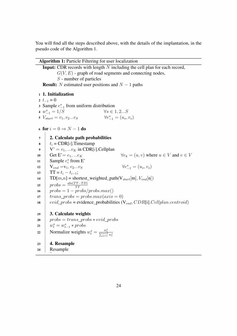
You will find all the steps described above, with the details of the implantation, in thepseudo code of the Algorithm 1.

Algorithm 1: Particle Filtering for user localizationInput: CDR records with length N including the cell plan for each record,

G(V,E) - graph of road segments and connecting nodes,S - number of particles

Result: N estimated user positions and N − 1 paths

1 1. Initialization2 t−1 = 03 Sample es−1 from uniform distribution4 ws

−1 = 1/S ∀s ∈ 1, 2...S5 Vstart = v1, v2...vS ∀es−1 = (us, vs)

6 for i = 0 −→ N − 1 do

7 2. Calculate path probabilities8 ti = CDR[i].Timestamp9 V’ = v1, ...vK in CDR[i].Cellplan

10 Get E’= e1, ...eK ∀ek = (u, v) where u ∈ V and v ∈ V11 Sample esi from E’12 Vend =v1, v2...vS ∀es−1 = (us, vs)13 TT = ti − ti−1;14 TD[m,n] = shortest_weighted_path(Vstart[m], Vend[n])

15 probs = abs(TT−TD)TT

16 probs = 1− probs/probs.max()17 trans_probs = probs.max(axis = 0)18 evid_probs = evidence_probabilities (Vend, CDR[i].Cellplan.centroid)

19 3. Calculate weights20 probs = trans_probs ∗ evid_probs21 ws

t = wst−1 ∗ probs

22 Normalize weights wst =

wst∑s=S

s=1 wst

23 4. Resample24 Resample

24

4 Experiments

This chapter will describe all the experiments done within the scope of this thesis andreport the results in the form of tables, figures, or graphs.

Acquiring real CDR data requires great effort and collaboration with MNO-s. Generally,it is possible for an individual to retrieve his personal record. However, in this case, wehave not removed all constraints as the general requests do not give the individuals theright to access information related to the cell borders. Only the MNO-s can provide thiskind of information. For this thesis, we received access to only a couple of hundreds ofrecords together with the cell shapes from one operator in Estonia. In order to overcomethe limitations of a small dataset we firstly decided to evaluate the method in syntheticdata. Additionally, by creating an experimental set up we will have almost full controlover the parameters of the system. We can evaluate the effect that each parameter has onthe outcome of the experiments. At the same time, during this process, we could see ifsome changes are necessary to help improve performance. The synthetic CDR data aregenerated taking into consideration public GPS trajectories. The prediction error afterrunning the algorithm is evaluated as in subsection "User positioning evaluation". Therewere three parameters that we explored the most. Firstly, we tried to estimate the effectof the particles on accuracy improvement. Later on, we analyzed the effect of the cellsurface and time granularity.

The second set of experiments is performed over real data. Here we keep constant thenumber of particles, meanwhile, the cell surface and time granularity are determinedby the dataset itself. Being that for this dataset we have the full GPS trace we add oneextra step on the evaluation, path accuracy. You will find the description of the metricused in this case in the subsection "Path evaluation". For the real data, it is necessarythat the trajectories are checked for any inconsistency that would affect the particle filter.We had such a case with long gaps between two records. The particle filtering bases itsprobability calculation in the traversal time TT and estimated time TD. In cases whenthe TT is considerably large compared to all TD-s, the algorithm will always define thelongest path as the most probable. In order to avoid this bias, we take two measures.Firstly, if the time difference between two consecutive records is more than three hourswe consider the trip to be finished. At this moment we interrupt the particle filteringalgorithm and restart it from the beginning using the new trajectory that starts from thesecond record. The second step we perform is calculating the time that is needed totraverse the most distant points between two cells. If this time is lower than the differencebetween two timestamps it means the user has stayed for a long time in one of the cellswithout any activity. In this case, we calculate TT as the time to traverse the path betweentwo centroids of the cells to avoid the bias towards the longest path.

25

4.1 Evaluation metrics

For our system, the GPS locations serve as the ground truth. Our main intention is to po-sition the user as close to the GPS position as possible. As an output from our algorithm,for every CDR record, we get a possible trajectory comprised of the most probable roadsegment that the user has followed from the previous to the present timestamp. The endnode of this path is our predicted user location. In order to evaluate the accuracy of ouralgorithm, we have to compare this location with the given GPS position. Additionally,as an extra step, we can evaluate if the predicted path is similar to the actual traversedpath. Below we are going to show the evaluation metrics for both cases.

User positioning evaluation

To evaluate our model we calculate the haversine distance [25] between our predicteduser location for the timestamp and the actual GPS location.

a = sin2(∆Φ

2) + cos(Φ1) · cos(Φ2) · sin2(

∆Λ

2) (7)

d = R · 2 · atan2(√a,√

1− a) (8)

Where Φ is the latitude, Λ is longitude, R is earth’s radius (mean radius = 6,371 km).d in our use case represents the error that the algorithm has made towards the ground truth.

Path evaluation

Given that we are provided with a full GPS trajectory in the time-span between thecapture of two CDR records, we can evaluate the accuracy of the proposed path from ouralgorithm for the user movement. Every GPS point in the trajectory is mapped to theclosest edge on the graph. The result is a list of edges that serve as the ground truth. Wefind the intersection between this list and the list proposed by the algorithm 1. Afterward,the accuracy is calculated as a ratio between the common elements of the list and totalelements in the GPS trajectory, expressed as a percentage.

Egps = e1, e2, ...ek

Epf = e1, e2, ...ej

26

Acc =len(Egps ∩ Epf )

len(Egps)· 100 (9)

4.2 Model evaluation in synthetic data

The first set of experiments were performed in a controlled setting. This section willdescribe how we generated the dataset, different parameters taken under observation, andthe outcomes for each.

4.2.1 Dataset description

The data used in this section belongs to the T-drive [26][27] dataset that contains aone-week GPS trajectory of 10,357 taxis in the city of Beijing. Due to time complexityrestrictions of the Particle Filter algorithm we have selected the trajectories of only twotaxis. In Figure 5 we can see the distribution of the taxis’ locations on top of Beijing citycenter map. The total 1972 data points are represented with two different colors, whichdistinguish the two taxis. For the rest of the thesis we are referring to this data as T-Drivedataset, nevertheless, this is only a small sample from the original data.

Figure 5. GPS data from T-drive dataset

In Figure 6 we can see the distribution of frequencies for the GPS records. Most of therecords are retrieved within less than five minutes from each other. In those 5 minutes,most of the time the taxis have traveled between 0 and 2 km.

27

Figure 6. Time and distance relation in T-drive dataset

After the visualization of the dataset, we have to construct our own CDR data. In orderto represent the cell coverage from MNOs we have split the geographical area into equalhexagons with diameter 1800 meters. The diameter is representative of most of the cellsin urban areas like Beijing city. A unique ID is given to each hexagon. In a second step,every GPS record is assigned to one of these hexagons. The data now has the featuresTimestamp, Longitude, Latitude, CGI, Cellplan and it is ready to be retrieved by thealgorithm 1. We are making the assumption that when a GPS event is triggered, a CDRevent is triggered automatically at the same time. Figure 7 visualizes the spread of thecells in the map together with the GPS points assigned to them.

Figure 7. CDR generated events from T-drive dataset

28

4.2.2 Results

We have selected to initialize the Particle Filter algorithm with 50 particles as a reasonablenumber considering the small size of the cells. The dataset corresponding to the twotaxis locations from T-drive project was fed to the algorithm together with the mapextracted from Open Street Map of the Beijing city. The results received are displayedin the histogram in Figure 8. The distribution is a positively skewed distribution witha mean 678 m and a standard deviation of 360 m. There are 81 records or 4.2% of thecases where the error is less than 100 m. Out of this, the minimum error is only 4.8 m.However, we have a maximum error of 1735.7 m as well.

Figure 8. Error distribution using 50 particles in generated CDR events

Sample sizeIn many particle filter applications, the number of particles used is set in an arbitraryway and kept constant throughout the application. Theoretically, when the number ofparticles increases near the infinity we are able to model the desired phenomena in aperfect way. Hence, we wanted to study the effect that the number of particles will havein the error for the user positioning. Due to the high time requirements for the executionof the algorithm, we have considered these levels: 3 particles, 20 particles, 50 particles,100 particles. The results are presented in Figure 9. When looking at the results we didnot notice a considerable difference when the number of particles changes. In 9 (a) wehave shown the cumulative distribution of the errors. Both axes are in logarithmic scaleto help with the comparison in the visualization. In 9 (b) we are showing the boxplotrepresentation of the errors.

29

(a) CDF (b) Boxplot

Figure 9. The effect of sample size

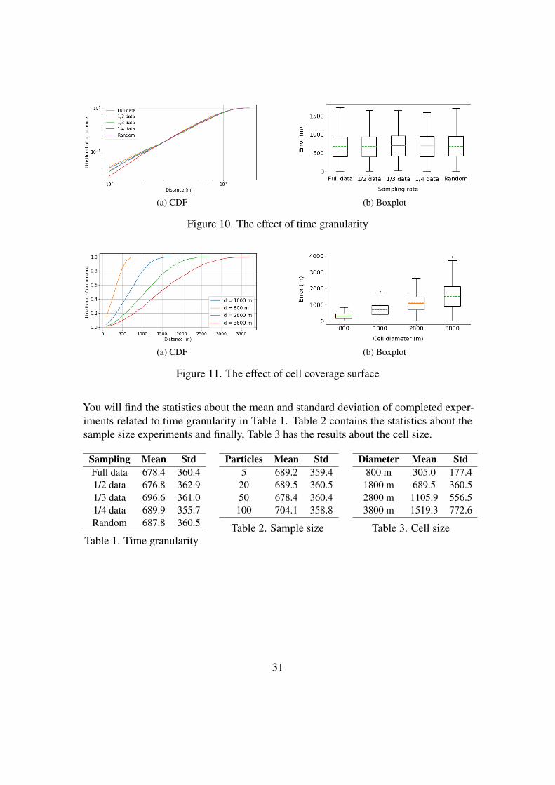
Time granularityAnother factor to consider when dealing with user positioning is the temporal uncer-tainties which are closely related to the time gaps between the generated CDR data. Inthis dataset, the time granularity of the CDR data, based on the applied assumption togenerate the synthetic data, is the same as with the GPS traces. We already presented itvisually in Figure 6. Most of the CDR events in this dataset are generated in less than5 minutes away from each other. However, nowadays the CDRs are not that frequentyet. Based on the increased usage of mobile devices, maybe in the future, this will bethe case. It was in our interest to understand what is the effect that the time granularityhas over the resulting errors. To quantify this effect we have used different levels of datasampling. The first sample was generated keeping every second record from the originaldataset, resulting in 963 records. As you can imagine most of the data now have a timedistance of fewer than 10 minutes. The second sample was generated taking every thirdrecord and the later one by keeping every fourth record. In addition to these regulatedsamples, we generated a random one. A random number (keep probability) between 0and 1 was drawn from the uniform distribution for every record in the CDR trajectory.If the number is higher than 0.5 we keep the record, otherwise we drop it. The resultsfrom our experiments using the newly created datasets with different sampling rates aredisplayed in Figure 10.

Cell sizesThe third factor we have to take into consideration is the spatial uncertainties. The errordistribution for user positioning is limited within the range of the longest diameter of thehexagon. However, these limits vary when it comes to MNO cell towers coverage. Wepreviously mentioned that the diameter ranges from some meters in the urban areas upto 30-40 km in rural areas. Hence, our next will be to study how the change in cell sizeaffects the distribution of our errors. We have tried four different levels of the diametersizes: 800 m, 1800 m, 2800 m and 3800 m that are suitable for an urban area like Beijingcenter. The results of the experiments are shown in Figure 11.

30

(a) CDF (b) Boxplot

Figure 10. The effect of time granularity

(a) CDF (b) Boxplot

Figure 11. The effect of cell coverage surface

You will find the statistics about the mean and standard deviation of completed exper-iments related to time granularity in Table 1. Table 2 contains the statistics about thesample size experiments and finally, Table 3 has the results about the cell size.

Sampling Mean StdFull data 678.4 360.41/2 data 676.8 362.91/3 data 696.6 361.01/4 data 689.9 355.7Random 687.8 360.5

Table 1. Time granularity

Particles Mean Std5 689.2 359.420 689.5 360.550 678.4 360.4100 704.1 358.8

Table 2. Sample size

Diameter Mean Std800 m 305.0 177.4

1800 m 689.5 360.52800 m 1105.9 556.53800 m 1519.3 772.6

Table 3. Cell size

31

4.3 Case study: Real CDR data

When it comes to similar applications we already mentioned that there is not enoughrelated work. However, the authors in [19][18], have taken the same problem underthe consideration and used the Switching Kalman Filter approach to solve it. We havereceived access to the dataset they used in their study and the results acquired.

4.3.1 Dataset description

The dataset consists of CDR data of five mobile owners in Estonia, accompanied by thefile with their GPS data locations. The period of data extraction is between April andAugust 2015. This dataset corresponds to a more realistic scenario from the previousdataset, and we can clearly detect that from Figure 12.

Figure 12. Time and distance relation in real CDR events

Most of the data are captured between every 0 and 500 minutes and the users have movedwithin that period from 0 to 20 km. It is easy to notice here the lack of information andthe challenges with real data we introduced at the beginning of the experiment section.For example, a user who traveled 0 km between two events that have a gap of 2500minutes can represent two cases. The first one would be that the user has not moved at allfrom his location i.e. the events are triggered in the evening and later in the morning. Inthis case, the user has been in his home location for the whole time. However, the secondcase is more complicated. The user might have traveled from the initial point A to pointB and came back to point A. During this period the two events are generated only whenstarting from point A and after returning to point A. However, we do not have any trace

32

for the intermediate event. Another challenging point is the users that traveled around 20km or more in almost 0 minutes. This happens in cases where there are problems withCDR data receiver and the timestamp is corrupted. The newly generated CDR recordwill be assigned to the last seen timestamp. This figure gives a good overview of thenature of real data. Moreover, some outliers were removed and not shown in the figure inorder to have better visualization.

In contrary to our previous example the level of uncertainty related to user positioning inthis dataset is significantly increased. In addition, the cell surfaces in real scenarios donot have a perfect hexagonal shape. Their shape resembles more of a distorted polygon orhexagon. One of the geographic information systems, called QGIS, was used to visualizethe coverage areas. In many cases, we could notice parts of them overlap with eachother. In Figure 13 we can see the distribution of the diameter of the cells in this dataset.Notice here, the diameter calculation is an approximation as the cells do not have regularhexagon or circular shape. We have calculated the surface of each cell and estimatedthe diameter of the largest circle we could create within this surface. The majority ofthe cells have a diameter of less than 1 000 m. This is expected as the majority of themovements of these users happen in the city. The rural cells vary from 5 000 to around25 000 in diameter which makes the user positioning task really challenging in thesecases.

Figure 13. Cell diameter distribution in real CDR events

In total the dataset had 699 records. We have run our algorithm using 20 particles throughthe complete chain of provided CDR traces. However, we noticed that some GPS recordsdid not fall into the cell area given for the same timestamp. This is normal in the caseswhere the GPS receiver was not always turned on or it was impossible to collect allthe GPS trajectories for the users. In this case, the closest GPS location in time with

33

the triggered CDR record is selected. This gap can be from several seconds to severalminutes and the user might have moved in a considerable distance. Due to the design ofthe particle filtering for mobile user localization a proper evaluation can be done onlywhen the GPS information matches the CDR. Hence, we have decided to exclude theother cases from the report and show the result only for 359 records.

In addition, for two out of five user IDs we had been provided with complete GPStrajectories of user movements. For these users, we performed the step of path evaluation.You can see the results of these experiments in the next section.

4.3.2 Results

Comparison with Switching Kalman FilterIn Figure 14 we have shown a comparison between the distribution of the results achievedby our particle filter application on user positioning and the results achieved by theproposed Switching Kalman Filter in [19]. The histogram represents bins of size 500meters. As we can see it seems the Switching Kalman Filter is performing better in thefirst bin. There are 220 elements grouped in contrary to 200 for Particle Filter. In thesecond bin, it seems there are more elements from Particle Filter and in the third, thesituation is the same. In general, Switching Kalman has a mean of 988 m and a standarddeviation of 1631 m. The Particle Filter has a mean of 1571 m and a standard deviationof 2586 m. We can see the particle filtering has more outliers with 5 present bins between10000 m and 17000 m while Kalman has only one bin.

Figure 14. Distribution of errors for Particle Filter and Switching Kalman Filter in realCDR data

34

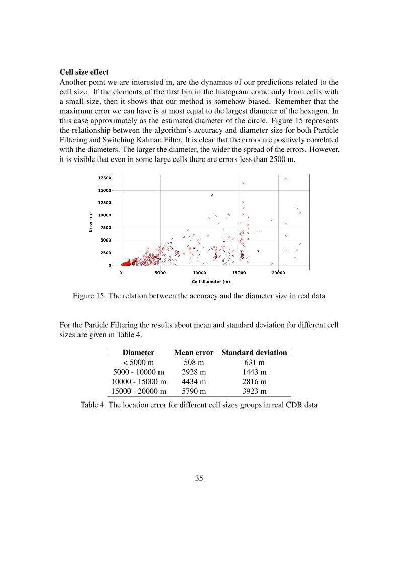
Cell size effectAnother point we are interested in, are the dynamics of our predictions related to thecell size. If the elements of the first bin in the histogram come only from cells witha small size, then it shows that our method is somehow biased. Remember that themaximum error we can have is at most equal to the largest diameter of the hexagon. Inthis case approximately as the estimated diameter of the circle. Figure 15 representsthe relationship between the algorithm’s accuracy and diameter size for both ParticleFiltering and Switching Kalman Filter. It is clear that the errors are positively correlatedwith the diameters. The larger the diameter, the wider the spread of the errors. However,it is visible that even in some large cells there are errors less than 2500 m.

Figure 15. The relation between the accuracy and the diameter size in real data

For the Particle Filtering the results about mean and standard deviation for different cellsizes are given in Table 4.

Diameter Mean error Standard deviation< 5000 m 508 m 631 m

5000 - 10000 m 2928 m 1443 m10000 - 15000 m 4434 m 2816 m15000 - 20000 m 5790 m 3923 m

Table 4. The location error for different cell sizes groups in real CDR data

35

Path evaluationFor almost half of the data, we were provided with full GPS trajectories. This allowedus to evaluate our predicted paths using the method presented in the section "PathEvaluation". The mapping of GPS location to the edges was really time-consumingbecause the GPS data were extracted every 1 second, and the road network graph ofEstonia had a hundred thousand of edges. Hence, we decided to use a sampling strategydepending on the size of GPS trajectories. I.E every 10th record in cases where there aremore than 500 GPS points in one trajectory. The loss of information is not a concern asthe GPS data was already really dense and the path accuracy formula considers GPS asground truth.

For Switching Kalman Filter the path predictions were not given. However, we estimatedthem to be the shortest path between every two consecutive user locations predictedby the model. The edges in the generated shortest path are then compared with theedges in the GPS trajectory. The results for both methods are shown in Figure 16. Mostof the accuracy values fall within the first bin of 10%. The rest of them seems to bealmost uniformly distributed. There are elements even in the last bin with 90 - 100%accuracy. The Switching Kalman filter has more elements in the first bin and less in thelast compared to Particle Filtering. The average accuracy for our method is 17% and forthe Switching Kalman Filter the average is 14%.

Figure 16. Path accuracy in real data

The two images in Figure 17 are extracted from the generated user trajectories by theparticle filter. In Figure 17 (a) the path accuracy is only 19%. The user, in this case,has moved within the same cell, which has a very large size. You can notice how itoverlaps with the smaller cells. Despite the wide coverage area, our algorithm has beenable to locate the user in the south of the cell, really close to the actual position. In

36

the second example, Figure 17 (b), the path is matching almost completely. It can benoticed that the GPS records, marked with red in this image, do not start exactly withinthe cell. We mentioned previously that one of the reasons might be that there are notenough GPS data during the time frame between two CDR events. A second reasonwas introduced in section 2.1 Global System for Mobile communication. Due to mobilenetwork functionalities, the mobile devices are not always connected to the closest basestation. Therefore, the GPS location is not within the cell.

(a) Path with accuracy 19% (b) Path with accuracy 87%

Figure 17. Examples of predicted trajectories from Particle Filtering compared to realGPS locations

In Figure 18 are displayed two random samples from path predictions of SwitchingKalman Filter. In the first subfigure (a) the path has an accuracy of only 15% and theprediction is far away from the real position. In subfigure (b) the method has achievedto depict almost perfectly the trajectory followed by the user. Both methods seem toperform better in cases where there is some movement episode with non-overlappingcells.

(a) Path with accuracy 15% (b) Path with accuracy 85%

Figure 18. Examples of predicted trajectories from Switching Kalman Filter comparedto real GPS locations

37

5 Discussions

This chapter will discuss the challenges and opportunities of the non-linear ParticleFiltering method. Furthermore, the insights that we derived from the experiments andthe future work will be described.

It was Gustafsson et al. [20] who first said that the mobile data could potentially beused for positioning, in particular with particle filtering. The paper dates from 19 yearsago and since then it seems that the researchers have been more interested in usingaggregated mobile data for fields like urban planning, transport mode detection, publichealth, crisis management similar to COVID-19 scenarios, etc. Today, it exists only onestudy which considers individual user positioning with CDR data. However, instead ofparticle filtering, this study uses the Switching Kalman Filter. In our knowledge, thisthesis is the first work that considers the implementation and evaluation of a non-linearSequential Monte Carlo Method like Particle Filtering for the task of user positioning,using only minimal information. The main drive behind this work was to understand ifit is possible to improve the positioning accuracy using a non-linear method comparedto existing linear methods. Any improvements in findings will lead to improved dataquality for passive human mobility analyses that use CDR information.

5.1 Insights from the implementation and the results of the experi-ments

During the implementation phase, it was clear that one important factor that influencesthe accuracy of this application is the correct prediction of the travel time between twonodes. Currently, we are calculating this metric using the road segment length and themaximum speed attribute attached to each edge in the data extracted from Open StreetMap. Nevertheless, a high percentage of edges are missing this attribute. For these cases,we have to consider a single default maximum speed that is not differentiated for thecity roads or highways. The selection of the default speed limit is arbitrary and tries totake into account the general knowledge about the transport legislation in the area ofinterest. This approach introduces a second approximation step in top of the particlefiltering which in itself provides approximate solutions. This is an important factor thataffects the path accuracy results that we received in Figure 16. It was our expectationthat the majority of predicted paths would not match the paths given by the GPS trace.First due to the approximate nature of Particle Filtering and secondly due to travel timeestimations.

38

Another important factor that should be taken into consideration is the nature of coverageareas. From the study case on CDR data collected in Estonia, we could see that theywere far from perfect. The coverage areas overlap with each other in a large portion andthe umbrella cells were present. Moreover, they were not always optimal. Many mobilephones were connected to some nearby cells that were not foreseen. This means that thecoverage areas provided by MNOs are not totally precise. One way to deal with themis by applying coverage optimization based on data-driven models like authors in [18],[19]. This approach has shown on average an improvement of 312 meters on error.

We have evaluated the effect of particle size on the results. In contrary to what the generaltheory of particle filtering describes and our expectations, a larger number of particles isnot producing considerable improvements. However, it seems that 50 particles work bestand the improvement stops when we increase the number to 100 particles. Nevertheless,from the CDF plot, we noticed that 100 particles have a higher likelihood in the firstbins compared to the other sampling levels. It means the higher number of particles, thehigher the probability that more elements will be in the first bins. There is a considerabledifference in execution time when using 100, 50, or 20 particles. Hence, a decision on thetrade-off between the improvements and the execution time is necessary. One interestingconfirmation that we received from the experiments was the fact that the time granularityof generated CDR records is related to the accuracy of the particle filtering. The worstperforming scenario was when only every fourth record was used in prediction. The lastinsight we had from this set of experiments was related to the cell sizes. There was anincrease of almost 400 meters in mean every time that we increased the cell diameterwith 1 000 m. When the cell was minimal (d = 800 m) we could see that the error wasconsiderably small.

The second set of experiments was performed in real data. From the comparison betweenour method and the non-linear Switching Kalman Filter we noticed that although theyproduce similar results, particle filtering in this dataset was not able to outperform theSwitching Kalman Filter. One characteristic that might impact positively the accuracy ofthe Kalman Filter is that it can depict the episode of Movement or Stay. Particle Filteringhas a lower chance to predict the same location twice, in case the user is not movingthroughout a series of records. First, because the newly sampled particles are selectedrandomly and the probability that some of them are similar to the last location dependshighly on cell sizes. And second, even if the previous stay location is duplicated in thenew set of particles, the probability that is selected again is high when the time gapbetween two events is small. The probability lowers when the time gap increases, whichmight be the case if the user is staying at home or office and does not use the mobile fora long time. Although we evaluated both methods in only 359 data points, it might benecessary to use a larger data-set to compare both methods for the results to be moregeneralizing.

39

Particle Filtering, in general, it is known to be a complex algorithm with high timerequirements. This is the main reason why the other methods are preferred in linearmodels with a normal noise, even though it would be totally possible to use particlefiltering as well. In this particular application, when we combine particle filtering methodswith the shortest path calculations in a large graph the time complexity increases. Evenafter parallel processing performed on the shortest paths calculations, Particle Filteringcontinues to be slow, especially compared to the Switching Kalman Filter.

5.2 Future work

Based on the discussion above we have identified the areas that can be improved in thismethodology.

First, there is a necessity to be able to better model the travel time, not depending onthe maximum speed limit only. The sophistication in the method we use for travel timeestimation can take into consideration the traffic situation, most common paths, trafficrules, etc. Therefore, we can model the spatial and temporal variations in speed. However,these models require access to large scale data of vehicle locations.

Second, in this thesis, we do not consider the separation between the pedestrian move-ments and the movements via different transportation modes. This is mainly due to thefact the data was coming only from moving vehicles. In future applications, it would bebeneficial to add one step that detects the mode of transportation and the output serves asan input for the travel time estimation.

Additionally, in order to reduce the temporal uncertainties before applying the particlefiltering model we can perform the step of trajectory reconstruction using one of the meth-ods introduced in the works of [15], [17] or [16]. For the spatial uncertainties encounteredwith not accurate cell shapes, it might be necessary to apply some preprocessing likecoverage area optimization or overlap detection.

Lastly, it will be interesting to see the results of applying the algorithm to real data withhigher quantity and quality.

40

6 Summary

Geo-localization is becoming an important feature of many applications and data analysisprojects and in many cases, it provides competitive advantages. Today the data extractedfrom Global Positioning System (GPS) are highly reliable, have high time precision(almost every second), and the first choice for real-time applications. On the otherhand domains like urban planning, tourism, public health etc. on have the need to havelarge scale mobility data, with low acquiring and processing costs. Unfortunately, thisis not possible with GPS data. Not all users are willing to share their GPS location.Furthermore, the data extraction and processing requires high power consumption. Thatis the reason why these domains are looking towards mobile data from Mobile NetworkOperators. Mobile data are retrieved from MNOs for billing purposes every time thatwe use our mobiles for calls, SMS, or 4/5G internet service. If we look at the datafrom all MNOs operating in a country we can extract the mobility patterns of all thecitizens within a given period. According to the studies and statistics the mobile usersare increasing in number as well as the CDR data frequency.

The quality of CDR data received from MNOs is closely related to the functionality ofthe mobile network. In Chapter 2 we gave an overview of the main standard for mobilenetworks, called GSM, and described its main components: Base station subsystem(BSS), Network switching subsystem (NSS), and Support subsystem (OSS). We describedhow the CDR event is triggered and its contents. Later on, we discussed the context inwhich the CDR can be used for user positioning and the spatial and temporal challengesthat come with it. In section 2.3 we saw that different research areas have embraced CDRdifferently. They are serving mostly as support data for other research topics like tourism,transportation, etc. Meanwhile, there were studies that were dealing with two mainchallenges of CDR: temporal and spatial uncertainties. The first group uses trajectoryreconstruction techniques and the second group deals with user positioning. We did takea look at the adaption of the particle filtering in localization and tracking problems andnoticed that nobody so far has used it for user positioning with CDR data. This thesiswill be the first method to use a nonlinear modeling technique like particle filtering foruser positioning.

Particle filtering concepts have their beginnings in a publication by Gordon et al.[23] in1993. Later on, the technique was improved and adopted in many fields. It falls underSequential Monte Carlo methods and is used to model nonlinear phenomena with notnormally distributed noise. The technique involves a set of particles that are drawn fromthe prior belief distribution. The main steps of the algorithm can be described as Predict,Update, and Reweigh. Our application follows the same phases to predict the locationand movements of a mobile user. The first step required CDR data and a map of edges

41

and nodes representing the road segment. The user position is predicted to be normallydistributed on the set of edges within the cell edges. A metric that correlates the actualtime between CDR records and the predicted traversal time of the path is used to decideon the weights of each particle. In the end, a resampling step is applied were the moreimportant particles are duplicated and the others are dropped.

We first tested our algorithm in an experimental setting using GPS data from taxis drivingin Beijing center. After applying the steps described in section 4.2 the CDR events weregenerated. There were three main parameters that we kept in control and evaluated theireffect on the algorithm accuracy: particle size, cell surface size, and time granularity. Theresults showed that in experimental settings the particle size did not have a significantimpact on the accuracy of the model. On the other hand, the time granularity and cellsize had a noticeable effect. Additionally, we evaluated the algorithm in a real case withdata from [19]. We compared our results with the results that authors of the same paperhave received. The results showed that our algorithm was performing at quite a similarscale but was not able to overcome their accuracy. Additionally, we have evaluated thepath accuracy in a portion of the data.

42

7 Conclusion

This thesis aimed to evaluate if it is possible to improve the accuracy of the user po-sitioning with mobile CDR data by introducing the adaptation of a non-linear particlefilter algorithm to the problem. Our proposed model was evaluated in synthetic andreal-case data. Based on the analysis we could conclude our approach was achievingsimilar results but not better compared to the previous linear techniques like SwitchingKalman Filter. Although, our method had a 3% higher accuracy in the path evaluation.The major factor affecting the accuracy of our method is the travel time estimation. Inthe future, it is necessary to sophisticate the travel time estimation approach by modelingspatial and temporal fluctuations in speed. In addition, it would be in the interest ofthis research to compare both methods in a larger data sample. Our proposed methodis completely new in a field that remains important for many areas and could be usefulin different scenarios, especially particular cases like public health. The main benefit isthe fact that it leverages mobile data, that have low extraction cost and are available forevery mobile user, with only basic features required.

43

References

[1] K. Boyini, “Global system for mobile communications,” 2018. [Online]. Available:https://www.tutorialspoint.com/global-system-for-mobile-communications

[2] The International Engineering Consortium, “Global system for mobilecommunication (GSM).” [Online]. Available: http://www.uky.edu/~jclark/mas355/GSM.PDF

[3] N. Deblauwe, GSM-based Positioning: Techniques and Applications, year = 2008.Asp / Vubpress / Upa.

[4] “Cell sizes.” [Online]. Available: http://www.wirelesscommunication.nl/reference/chaptr04/cellplan/cellsize.htm

[5] A. Turner, “1 billion more phones than people in the world,” 2018. [Online].Available: https://www.bankmycell.com/blog/how-many-phones-are-in-the-world

[6] P. Fiadino, V. Ponce-Lopez, J. Antonio, M. Torrent-Moreno, and A. D’Alconzo,“Call detail records for human mobility studies: Taking stock of the situation in the“always connected era”,” in Proceedings of the Workshop on Big Data Analyticsand Machine Learning for Data Communication Networks, ser. Big-DAMA ’17.New York, NY, USA: Association for Computing Machinery, 2017, p. 43–48.[Online]. Available: https://doi.org/10.1145/3098593.3098601

[7] M. Lebdi, “What happens to your data when you make acall ?” 2019. [Online]. Available: https://medium.com/sfu-cspmp/what-happens-to-your-data-when-you-make-a-call-f05812da4f8d

[8] T. Vajakas and J. Rõõmusaare, “On optimal spatial probability density estimationof passive mobile positioning events,” in 2016 15th Biennial Baltic ElectronicsConference (BEC), 2016, pp. 127–130.

[9] R. Sikder, M. Uddin, and S. Halder, “An Efficient Approach of Identifying Touristby Call Detail Record Analysis,” 2016.

[10] E. Saluveer, J. Raun, M. Tiru, L. Altin, J. Kroon, T. Snitsarenko, A. Aasa,and S. Silm, “Methodological framework for producing national tourismstatistics from mobile positioning data,” Annals of Tourism Research, vol. 81, p.102895, 2020. [Online]. Available: http://www.sciencedirect.com/science/article/pii/S0160738320300396

44

[11] S. Qin, J. Man, X. Wang, C. Li, H. Dong, and X. Ge, “Applying Big Data Analyticsto Monitor Tourist Flow for the Scenic Area Operation Management,” DiscreteDynamics in Nature and Society, vol. 2019, pp. 1–11, 2019.

[12] G. Khodabandelou, V. Gauthier, M. El-Yacoubi, and M. Fiore, “Population esti-mation from mobile network traffic metadata,” in 2016 IEEE 17th InternationalSymposium on A World of Wireless, Mobile and Multimedia Networks (WoWMoM),June 2016, pp. 1–9.

[13] M. Friedrich, K. Immisch, P. Jehlicka, T. Otterstätter, and J. Schlaich, “GeneratingOrigin-Destination Matrices from Mobile Phone Trajectories,” TransportationResearch Record: Journal of the Transportation Research Board, vol. 2196, pp.93–101, 2010.

[14] M. Pourmoradnasseri, K. Khoshkhah, A. Lind, and A. Hadachi, “OD-MatrixExtraction based on Trajectory Reconstruction from Mobile Data,” 2019.

[15] S. Hoteit, S. Secci, S. Sobolevsky, C. Ratti, and G. Pujolle, “Estimating humantrajectories and hotspots through mobile phone data,” Computer Networks, vol. 64,pp. 296–307, 2014. [Online]. Available: http://www.sciencedirect.com/science/article/pii/S1389128614000656

[16] G. Chen, A. Viana, M. Fiore, and C. Sarraute, “Complete Trajectory Reconstructionfrom Sparse Mobile Phone Data,” EPJ Data Science, vol. 8, 2019.

[17] T. Vajakas, J. Vajakas, and R. Lillemets, “Trajectory reconstruction from mobilepositioning data using cell-to-cell travel time information,” International Journal ofGeographical Information Science, vol. 29, no. 11, pp. 1941–1954, 2015. [Online].Available: https://doi.org/10.1080/13658816.2015.1049540

[18] A. Lind, A. Hadachi, and O. Batrashev, “A new approach for mobile positioningusing the cdr data of cellular networks,” in 2017 5th IEEE International Confer-ence on Models and Technologies for Intelligent Transportation Systems (MT-ITS).IEEE, 2017, pp. 315–320.

[19] A. Hadachi and A. Lind, “Exploring a New Model for Mobile Positioning Basedon CDR Data of The Cellular Networks,” 2019.

[20] F. Gustafsson, F. Gunnarsson, N. Bergman, U. Forssell, J. Jansson, P. . Nordlund,and R. Karlsson, “A framework for particle filtering in positioning, navigation andtracking problems,” in Proceedings of the 11th IEEE Signal Processing Workshopon Statistical Signal Processing (Cat. No.01TH8563), Aug 2001, pp. 34–37.

45

[21] L. Hu and D. Evans, “Localization for mobile sensor networks,” in Proceedings ofthe 10th Annual International Conference on Mobile Computing and Networking,ser. MobiCom ’04. New York, NY, USA: Association for Computing Machinery,2004, p. 45–57. [Online]. Available: https://doi.org/10.1145/1023720.1023726

[22] B. Dil, S. Dulman, and P. Havinga, “Range-Based Localization in Mobile SensorNetworks,” in European Conference on Wireless Sensor Networks, 2006, pp. 164–179.

[23] A. F. M. Smith, “Novel approach to nonlinear/non-Gaussian Bayesianstate estimation,” IEE Proceedings F (Radar and Signal Processing),vol. 140, no. 2, pp. 107–113(6), apr 1993. [Online]. Available: https://digital-library.theiet.org/content/journals/10.1049/ip-f-2.1993.0015

[24] K. P. Murphy, Machine learning: a probabilistic perspective, ser. Adaptive compu-tation and machine learning series. Cambridge, MA: MIT Press, 2012.

[25] D. Neff, “Deriving the Haversine Formula,” apr 1999. [Online]. Available:http://mathforum.org/library/drmath/view/51879.html

[26] Y. Zheng, “T-Drive trajectory data sample,” aug 2011. [Online]. Available: https://www.microsoft.com/en-us/research/publication/t-drive-trajectory-data-sample/

[27] J. Yuan, Y. Zheng, X. Xie, and G. Sun, “Driving with knowledge from the physicalworld,” in Proceedings of the 17th ACM SIGKDD International Conference onKnowledge Discovery and Data Mining, ser. KDD ’11. New York, NY, USA:Association for Computing Machinery, 2011, p. 316–324. [Online]. Available:https://doi.org/10.1145/2020408.2020462

46

II. Licence

Non-exclusive licence to reproduce thesis and make thesis public

I, Salijona Dyrmishi,

1. herewith grant the University of Tartu a free permit (non-exclusive licence) to

reproduce, for the purpose of preservation, including for adding to the DSpacedigital archives until the expiry of the term of copyright,

Creating a novel approach for mobile positioning based on CDR data,

supervised by Amnir Hadachi, PhD.

2. I grant the University of Tartu a permit to make the work specified in p. 1 availableto the public via the web environment of the University of Tartu, including viathe DSpace digital archives, under the Creative Commons licence CC BY NCND 3.0, which allows, by giving appropriate credit to the author, to reproduce,distribute the work and communicate it to the public, and prohibits the creation ofderivative works and any commercial use of the work until the expiry of the termof copyright.

3. I am aware of the fact that the author retains the rights specified in p. 1 and 2.

4. I certify that granting the non-exclusive licence does not infringe other persons’intellectual property rights or rights arising from the personal data protectionlegislation.

Salijona Dyrmishi13/05/2020

47