university of trieste - international centre for ... · 1. de nition of the rankine vortex. the...

PhD - Environmental Fluid Mechanics - Physics of the Atmosphere

University of Trieste - International Centre for Theoretical Physics

1

The Rankine Vortex Model

By DARIO B. GIAIOTTI1† AND FULVIO STEL1

1Regional Meteorological Observatory, via Oberdan, 16/A I-33040 Visco (UD), ITALY

(4 October 2006)

The Rankine vortex model is a circular flow in which an inner circular region about

the origin is in solid rotation, while the outer region is free of vorticity, the speed being

inversely proportional to the distance from the origin. This flow model has occasionally

been used for the wind distribution in a hurricane and in a tornado.

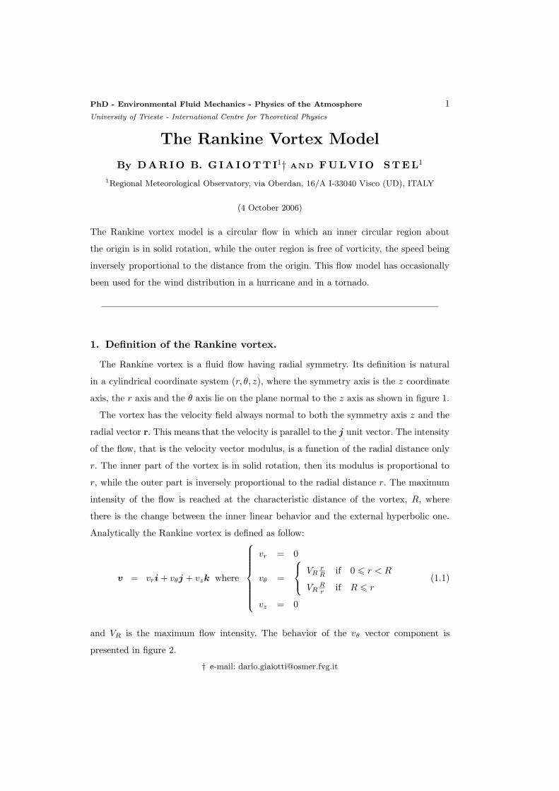
1. Definition of the Rankine vortex.

The Rankine vortex is a fluid flow having radial symmetry. Its definition is natural

in a cylindrical coordinate system (r, θ, z), where the symmetry axis is the z coordinate

axis, the r axis and the θ axis lie on the plane normal to the z axis as shown in figure 1.

The vortex has the velocity field always normal to both the symmetry axis z and the

radial vector r. This means that the velocity is parallel to the j unit vector. The intensity

of the flow, that is the velocity vector modulus, is a function of the radial distance only

r. The inner part of the vortex is in solid rotation, then its modulus is proportional to

r, while the outer part is inversely proportional to the radial distance r. The maximum

intensity of the flow is reached at the characteristic distance of the vortex, R, where

there is the change between the inner linear behavior and the external hyperbolic one.

Analytically the Rankine vortex is defined as follow:

v = vri + vθj + vzk where

vr = 0

vθ =

VRrR

if 0 6 r < R

VRRr

if R 6 r

vz = 0

(1.1)

and VR is the maximum flow intensity. The behavior of the vθ vector component is

presented in figure 2.

† e-mail: [email protected]

2 D. B. Giaiotti and F. Stel

Figure 1. The cylindrical coordinate system adopted for the description of the Rankine vortex

model. The unit normal vectors set (i, j,k) is reported in the point identified by coordinates

(r, θ, z).

2. The vorticity field

One of the main features of the Rankine vortex is its vorticity field. In fact according to

the definition of the vortex velocity field (1.1) and the the application of the curl operator

in cylindrical coordinates (A 4), it is evident that the vortex presents vertical vorticity

component only. Furthermore the vorticity field modulus is constant in the inner part of

the vortex, it is positive and it is a function of the maximum flow velocity and the vortex

characteristic distance only. In the outer region of the vortex, the flow has no vorticity

at all.

∇× v = k1

r

∂(rvθ)

∂r= k (

vθ

r+

∂vθ

∂r) = k

2VR

Rif 0 6 r < R

0 if R 6 r(2.1)

It is worth to note that the Rankine vortex is characterized by a continuous velocity

field, but with a discontinuity in vorticity at the characteristic distance. This has relevant

consequences on the turbulence in that region of the domain Batchelor (1993).

3. Applications of the model to atmospheric systems

The Rankine vortex is a simple model, but it can be considered suitable for the descrip-

tion of some typical atmospheric phenomena. Nowadays, thanks to the Doppler radar

measurements, several cases of well organized convective cell, named mesocyclones, have

been observed and the corresponding velocity fields have been measured. Mesocyclones

can be approximated to cylindrical rotating convective structures having a inner core of

The Rankine Vortex Model 3

0

0.2

0.4

0.6

0.8

1

1.2

0 1 2 3 4 5 6 7

v/V

R

r/R

v(r)

Figure 2. The Rankine vortex model is characterized by a flow that is always and everywhere

parallel to the j unit vector, so the only non null vector component is the vθ which is also the

total velocity vector modulus. In this figure the normalized velocity vector modulus (v/VR) is

plotted against the normalized radial distance (r/R). Note that at the characteristic distance R

there flow is continuous, but the flow regime changes, form a solid rotation for 0 6 r < R to a

hyperbolic decrease at distances greater or equal than R.

about 5 km diameter that is in solid rotation and an outer rotating region in which the

velocity drops with a law very close to the inverse of the distance. The peak velocity of

the mesocyclone is reached at its characteristic distance, the external border of the inner

core, and accounts of several meters per second, generally speeds larger than 10ms−1

have been measured and very often more than 20ms−1, see Bertato et al. (2003) and

Brown et al. (2005) as examples.

In figure 3 is reported the comparison between Doppler radar measurements, of a meso-

cyclone observed by means of the WSR-88D Doppler radar network, which is operating

in the United States, and a Rankine model of the mesocyclone Brown et al. (2005).

Tornadoes, see figure 4, present the Rankine vortex structure, even if the vortex struc-

ture has a quick dynamics, evolving form the early no vortex stage to its end in a few

minutes. The radial profile of the tangential, (vθ) (azimuthal), wind component has been

measured in several cases of tornado, by means of mobile Doppler radars and it shows

the typical Rankine vortex model, see figure 5 Brown et al. (2005). Of course the tor-

nado is characterized by a non null radial component of the wind (vr), especially at the


Figure 3. Doppler radar measurements, of a mesocyclone observed by means of the WSR-88D

Doppler radar network operating in the United States, and a Rankine model of the mesocyclone.

Velocities in ms−1 are reported along the ordinate, while in abscissa there is the distance from

the mesocyclone axis in km. Positive speeds represents radial velocities measured outward the

radar, negative speeds are velocities toward the radar. Figure thaken from the paper Brown

et al. (2005). Measurements of Doppler mesocyclone velocity across the mesocyclonic structure

are marked by solid black dots, while Rankine model profile is the solid curve with pointed

peaks. The smoother curve passing through the measurement points represents a model of wind

profile if the radar were able to measure in a continuous manner across the mesocyclone.

ground boundary. The radial component is usually an order of magnitude smaller than

the tangential one, as shown in the sequence of measurements presented in the figure 6,

where six snapshots of a tornado radial and azimuthal velocities have been taken about


Figure 4. Picture of the tornado whose measures are reported in figures 5 and 6. The tornado

occurred in Bassett, Nebraska, on June 1999. Figure taken form the Bluestein et al. (2003)

paper.

every 20 seconds. Positive radial wind values mean radial outflow, while negative ones

correspond to radial inflow.

From those figures it is possible to note the increase of the azimuthal wind speed

from the tornado center, qualitatively similar to the solid rotation part of the Rankine

vortex, and the wind speed decrease after the characteristic distance. For this tornado, the

characteristic distance (R) is about 0.2 km, as one can guess from figures 5 and 6 looking

at the radial distance where the tangential velocity gets its maximum value. It is worth to

note that the maximum tangential velocity is close to 30ms−1. Information concerning

the central part of the vortex, that is for r < 0.1 km, are not available because the were

no enough scatterers allowing the radar signal to be significantly reflected backward to

the receiver.

Even if qualitatively the Rankine vortex model fits the radial behavior of the tornado

azimuthal velocity, quantitatively the deviation from the Rankine model is evident in the

vorticity field as computed from the data, see figure 9. The time evolution of the vorticity

vertical component, computed according to the third term of the right hand side of the

formula A 4, does not characterize the tornado by a simply two regions constant field, that

is the constant vorticity inner core and an outer null vorticity environment, separated by

a discontinuity. As shown in the sequence of figure 9, the transition from the inner high


Figure 5. Averaged azimuthal and radial wind speeds over the most intense 40 seconds of

the tornado existence. Azimuthal wind component measurements are plotted as filled triangles,

connected with a solid line. Their scale, in ms−1 is reported on the left. Open circles connected

with a dashed line report the radial component of the tornado velocity. The corresponding scale

in ms−1 is on the right of the plot. Figure taken form the Bluestein et al. (2003) paper.

vorticity region, |∇ × v| ' 0.3 s−1, to the close to zero vorticity outer region is revealed

by several measurement points and covers a space comparable with the inner vortex core

R.

The smallest structures showing a Rankine vortex signature are the dust devils. These

vortexes take place in clear sky and fair weather conditions and usually they do not


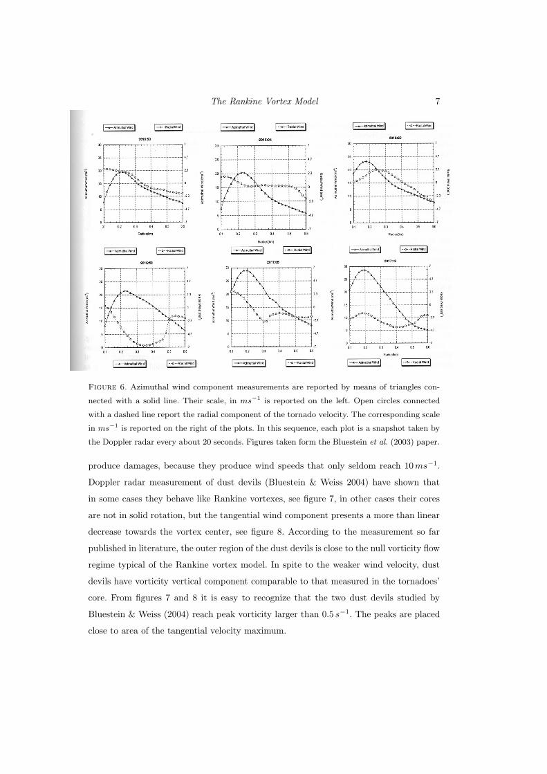
Figure 6. Azimuthal wind component measurements are reported by means of triangles con-

nected with a solid line. Their scale, in ms−1 is reported on the left. Open circles connected

with a dashed line report the radial component of the tornado velocity. The corresponding scale

in ms−1 is reported on the right of the plots. In this sequence, each plot is a snapshot taken by

the Doppler radar every about 20 seconds. Figures taken form the Bluestein et al. (2003) paper.

produce damages, because they produce wind speeds that only seldom reach 10ms−1.

Doppler radar measurement of dust devils (Bluestein & Weiss 2004) have shown that

in some cases they behave like Rankine vortexes, see figure 7, in other cases their cores

are not in solid rotation, but the tangential wind component presents a more than linear

decrease towards the vortex center, see figure 8. According to the measurement so far

published in literature, the outer region of the dust devils is close to the null vorticity flow

regime typical of the Rankine vortex model. In spite to the weaker wind velocity, dust

devils have vorticity vertical component comparable to that measured in the tornadoes’

core. From figures 7 and 8 it is easy to recognize that the two dust devils studied by

Bluestein & Weiss (2004) reach peak vorticity larger than 0.5 s−1. The peaks are placed

close to area of the tangential velocity maximum.


Figure 7. Radial profiles for a dust devil occurred in Texsas on May 1999 and observed by means

of a mobile Doppler radar. The solid black line reports the tangential velocity of the vortex in

ms−1. The vertical component of the vorticity is plotted in dashed line and it is expressed in

units of ×10 s−1. The dotted line represents the relative radar reflectivity; this variable is not

relevant in the context of this lecture so it is not describe in this caption. Picture taken from

the Bluestein & Weiss (2004) paper.

Take your notes here below


Figure 8. As in figure 7, but for another dust devil, which was observed in the same day of

that presented in figure 7, but more intense. Picture taken from the Bluestein & Weiss (2004)

paper.



Figure 9. Time series of the vorticity vertical component for the June 1999 Bassett, Nebraska,

tornado. The figures show the radial behavior of the vorticity, that was computed from the

Doppler radar data according to the third term of the right hand side of the formula A 4,

Vorticity is reported along the ordinate axis in 10−3 s−1 units, while the abscissa axis gives the

distance from the tornado center in km.



Figure 10. The general orthogonal curvilinear coordinate system. Unit vectors tangent to

the coordinate lines (i, j, k) are normal to each other in every point of the space. The el-

ementary displacements along coordinate lines are functions of the elementary coordinate

displacements (dx, dy, dz) and of the point where they are computed through the functions

α(x, y, z), β(x, y, z), γ(x, y, z).

Appendix A. The curl operator in cylindrical coordinates

Following the general expression for the curl operator in three-dimensional orthogonal

curvilinear coordinates (x, y, z), see figure 10, defined by means of the Euclidean metric

as follow:

ds2 = (α dx)2 + (β dy)2 + (γ dz)2 (A 1)

the operator is defined by means of the determinant notation (Batchelor 1994, see Ap-

pendix 2):

∇× F =1

αβγ

∣

∣

∣

∣

∣

∣

∣

∣

∣

αi βj γk

∂∂x

∂∂y

∂∂z

αFx βFy γFz

∣

∣

∣

∣

∣

∣

∣

∣

∣

(A 2)

Applying this general result to the cylindrical coordinate system, see figure 1, which is

characterized by (Batchelor 1994, see Appendix 2) and (Fogiel 2001, see Chalper 9)

α = 1 β = r γ = 1 (A 3)

then the curl components are as follow:

∇× F = i

[

1

r(∂Fz

∂θ−

∂(rFθ)

∂z)

]

+ j

[

∂Fr

∂z−

∂Fz

∂r

]

+ k

[

1

r(∂(rFθ)

∂r−

∂Fr

∂θ)

]

(A 4)


Appendix B. Exercises

B.1. Exercise 1

Consider the Rankine vortex model (1.1) and add to it a constant flow, then compute

the vorticity field. Is the vorticity changed? The consider a mesocyclone or a tornado at

the mid latitudes which is described by a Rankine vortex model, add to it a synoptic

flow and compute its potential vorticity. What about the vorticity of a tropical cyclone

described by a Rankine vortex model and moving from the tropics to the mid latitudes?

See (Crisciani 2005, cap. 7), Dutton (1995), Gill (1982), Holton (1972a), Pedlosky (1987).

B.2. Exercise 2

Consider the Rankine vortex model (1.1), compute and plot the trajectories for a set

three fluid parcels having initial conditions: (0, 0, 0), (R/2, 0, 0) and (2R, 0, 0). Then add

to the Rankine vortex model a constant flow a recompute and plot the trajectories for

the same three parcels.

B.3. Exercise 3

With reference to the figure 5, in particular using the maximum azimuthal velocity VR

and the corresponding characteristic vortex radius R, assume that the tornado is in

cyclostrophic balance, Giaiotti & Stel (2005), Holton (1972b), at r = R, then compute

the radial component of the pressure gradient in that point. Furthermore, assuming the

Rankine vortex model, compute the overall pressure difference between the characteristic

distance region and the center of the tornado. Use the VR value deduced by figure 5 and

assume that at r = R the atmospheric pressure is 1013.0hPa.


Appendix C. Historical notes

C.1. William John Macquorn Rankine

Born: 1820 in Edinburgh, Great Britain.

Died: 1872 in Edinburgh, Great Britain.

William John Macquorn Rankine, a Scottish engineer and physicist, contributed signif-

icantly to the thermodynamics. Rankine developed a fully complete theory of the steam

engine furthermore his interests were varied and in many branches of mathematics and

engineering.

Rankine interpreted the results of his molecular theories in terms of energy and its

transformation. That lead him to the energetics which gave an account of dynamics in

terms of energy and transformation rather than force. Energetics offered Rankine an

alternative approach, to his thermodynamics studies reducing the use of the molecular

vortexes method he developed earlier. He considered inadequate the theories of heat

proposed by Clausius and James Clark Maxwell, that are based on linear atomic motion.

It was only in 1869 that Rankine admitted the success of these rival theories. He used

his own theories to develop a number of practical results and to elucidate their physical

principles. Interesting is his contribution on the study of shock waves are important


REFERENCES

Batchelor, G. K. 1993 The theory of homogeneous turbulence. Cambridge University Press,

London.

Batchelor, G. K. 1994 An Introduction to Fluid Dynamics. Cambridge University Press,

London, New York, Melbourbne.

Bertato, M., Giaiotti, D. B., Manzato, A. & Stel, F. 2003 An interesting case of tornado

in friuli-northeastern italy. Atmospheric Research 7–68, 3–21.

Bluestein, H. B., Lee, W., Bell, M., Weiss, C. C. & Pazmany, A. L. 2003 Mobile doppler

radar observations of a tornado in a supercell near bassett, nebraska, on 5 june 1999. part

ii: Tornado-vortex structure. Mon. Wea. Rew. 131, 2968–2984.

Bluestein, H. B. & Weiss, C. C. 2004 Doppler radar observations of dust devils in texas.

Mon. Wea. Rew. 132, 209–224.

Brown, R. A., Flikinger, B. A., Forren, E., Schultz, D. M., Sirmans, D., Spencer,

P. L., Wood, V. T. & Ziegler, C. L. 2005 Improved detection of severe storms using

experimental fine-resolution wrs-88d measurements. Wea. Forecasting 20, 3–14.

Crisciani, F. 2005 Lecture notes on Geophysical Fluid Dynamics - PhD course on Environ-

mental Fluid Mechanics - ICTP/University od Trieste.

Dutton, J. A. 1995 Dynamics of the Atmosphere motion, chap. 7. Meteorological equations of

motion. Dover Publication Inc., New York.

Fogiel, M. 2001 Handbook of Mathematical, Scientific and Engineering formulas, tables, func-

tions, graphs, transforms. Reesearch & Education Association.

Giaiotti, D. B. & Stel, F. 2005 The natural coordinate system and its applications in at-

mospheric physics - PhD course on Environmental Fluid Mechanics - ICTP/University od

Trieste.

Gill, A. E. 1982 Atmosphere - Ocean Dynamics, chap. 4.10, p. 84. Academic Press, London.

Holton, J. R. 1972a An Introduction to Dynamic Meteorology , 3rd edn., chap. 2.2 The vectorial

form of the momentum equation in rotating coordinates. Academic Press, San Diego, CA.

Holton, J. R. 1972b An Introduction to Dynamic Meteorology , 3rd edn. Academic Press, San

Diego, CA.

Pedlosky, J. 1987 Geophysical Fluid Dynamics. Springer-Verlag, New York.

university of trieste - international centre for ... · 1. de nition of the rankine vortex. the...

Documents