University of Wisconsin-Madison \ i - 7.4

Institute for Research on Poverty Discussion Papers

G o r d o n H. L e w i s R i c h a r d J. M o r r i s o n

INTERACTIONS AMONG SOCIAL WELFARE PROGRAMS

I n s t i t u t e f o r Research on Poverty Discussion Paper no. 866-88

Interac tionr among Socia 1 Welfare Programs

Gordon H. Lewis Carnegie Me1 lon University

Richard J. Morrison Health and Welfare, Canada

September 1988

This research was supported i n pa r t by a grant t o the I n s t i t u t e f o r Research on Poverty, University of Wisconsin, from the U.S. Department of Health and Human Services. he opinions and conclusions expressed i n t h i s paper a r e those of the authors and do not necessari ly r e f l e c t the opinions o r policy of Carnegie Mellon University, the Department of Health and Welfare, Canada, the I n s t i t u t e f o r Research on Poverty, or the U.S. Department of Health and Human Services. The authors appreciate the comments by Michael Wiseman and Daniel Weinberg on an e a r l i e r version of t h i s paper.

The ~ n s t i t u t e ' s Discussion Papers s e r i e s is designed to describe, and to e l i c i t comments on, work i n progress. I ts papers should be considered working d r a f t s .

Abstract

Social welfare is affected not only by individual programs such as AFDC, food stamps, and Medicaid but by the interactions among such programs and the interactions between these benefit programs and the taxation system, including not only federal income tax, but FICA, the dependent care tax credit, the earned income tax credit, and state and local income taxes. As a prelude to understanding how the welfare system works, this paper explores several specific ways in which such programs interact. It illustrates four different types of interactions: the effect of one program on another; the effect of one program on the whole set of additional programs; the system of interacting tax and benefit reduction rates that jointly determine the cumulative marginal tax rate on income; and finally the effects of interacting programs on the governments that create and maintain those programs.

There are at least three benefits in analyzing such interactions. First, such analysis draws attention to the complex ways in which programs affect one another; second, it illustrates that the analysis of complex interactions such as this can be done; and third, it provides some substantive knowledge about the nature of the present system that should be useful as issues of welfare reform are pursued.

Interactions among Social Welfare Programs

1. Introduction The "welfare system" has once again become the focus of proposals for change. At least eight

different groups, ranging from the President's Domestic Policy Council, the Congressional Budget Office, and the General Accounting Office to the Ford Foundation and the Urban League have issued analyses of, or plans for, welfare reform. It is also clear that for the most part the present system, as a system, is not well understood. There are several reasons why this is so. First, there is not one system but many systems, depending on the part of the population that one is interested in. Second, the regulations controlling individual programs are often extensive. And third, the programs that make up any given "system" interact in complex ways.

In "Up from Dependency: A New National Public Assistance Strategy," the President's Domestic Policy Council (1 986) states:

Thinking about these programs (AFDC, food stamps, and Medicaid, for example) as separate entities, however. does not help us understand how they work in the real world. In that world, and especially from the viewpoint of the welfare recipient, all of these programs combine to operate as a single complex and bewildering system. Even though each program was designed to meet some specific need, together they interact to produce a system of conflicting rules and benefits. (p. 27)

Although that report ignores the fact that the set of programs changes as one considers different portions of the population, still the point made is valid: it is sets of programs not individual programs that affect recipients. Yet the individual programs within any given set are seldom analyzed or understood in a coordinated way.

If appropriate changes are to be made to the welfare system it would be good to have a thorough understanding of how the system works, what the interactions are, and what the overall effects on the system are. This paper focuses on some of the basic types of interactions among the major programs that determine the effective social welfare system for low-income families with children.

1.1. Complexlty and Unlntended Consequences The nature of the complexity of the present system for low-income families with children is illustrated in

Figure 1-1, which shows the major programs and factors that determine disposable income for such a family.' The circles represent income components and the principal taxitransfer programs with which the family interacts. The lines indicate that relationships exist between the elements. The negative sign on the line from earned income to AFDC, for example, indicates that as earned income increases AFDC benefits decrease. The negative sign on the line between earned income and food stamps indicates that as earned income increases food stamp benefits decrease, and the negative sign on the line between AFDC and food stamps means that as AFDC decreases, cetens paribus, food stamps increase. Thus, in ascertaining the effect of an increase in earned income on food stamps, one has to consider both the

'"~isposable income" as we shall use it in this paper refers to the sum of earned and unearned income, transfers from benefit programs including AFDC. the earned income tax credit, food stamps, and Medicaid, with both of these last two treated as if they were cash benefits. and minus the amounts paid in taxes: federal income tax after the dependent care expense tax credit, state income tax, and FICA. Since we include the insurance value of Medicaid as if it were a cash benefit, it might be more appropriate to think of the total as "effective income" rather than "disposable income," but we shall use the two terms interchangeably.

direct effect of the decrease in food stamps from the increase in earnings and the indirect effect of the increase in food stamps from the decrease in AFDC benefits, which in turn was caused by the increase in earned income and the earned income tax credit.*

Figure 1-1: Relationships among Transfer Components

- FIT Federal Injome Tax

AFDC Aid to Families wi th Dependent Children FS Food Stamps

CRDT Dependent Care Tax Credi t MED Medicaid

DYCR Day Care Expenses NET Net Income

EARN ~a rned Income OTHR Other Income

ElTC Earned lncome Tax Credi t SHLT Excess Shelter Costs

FICA Social Secur i ty Contribution SIT State Income Tax

In reality, however, the situation is more complex than shown in Figure 1-1 because programs are influenced by a variety of elements, limits, and specific regulations that affect programs in specific ways, not in a general or overall way. In the food stamp program, for example, the benefit is affected by dependent care expenses and the maximum allowable dependent care expense; it is affected by the portion of the total income that is based on earnings; it is affected by whether there are elderly in the household; and it is affected by the amount spent for shelter expenses, to the extent that such expenses exceed 5O0I0 of the net household income.

The result is a system that is sufficiently complex that, other than some of the microsimulation work that

'Figure 1-1 also shows that AFDC is affected by the earned income tax credit, and the earned income tax credit is affected by AFDC. The nature of this joint dependency is explained in the appendix, which discusses the modeling of the various programs.

has been done, most analyses focus on either a single program or a small number of program^.^ Most stop short of attempting to present comprehensive views of the interactions. In work done for the Joint

Economic Committee in 1972, one of the analysts suggested that to really understand the welfare system would require that one understand not only the interactions among various welfare programs but the interactions between the welfare system and the taxation system (Storey, 1972). In those analyses, however, that goal was considered beyond what could reasonably be accomplished. In 1987 when the Domestic Policy Council stressed the interactive nature of the welfare system, they too failed to include in their analyses the effects of tax programs.

In the current paper we shall present examples of four types of interaction that occur among programs within the system that affects low-income families with children. Before presenting these four examples, however, we provide a brief description of the methodology that was used and some general information about the models that were built. More detail about the operation of the welfare and taxation programs as we have modeled them is contained in the appendix.

1.2. Methodology The work presented in this paper utilizes MAPSIT, a computer package designed for the analysis of

systems consisting of interdependent, piecewise-linear functions. Like various microsimulation models (for example, TRIM and DYNASIM), MAPSIT operates on a microanalytic basis. Unlike the standard microsimulation models, however, MAPSIT allows the analyst to model many different types of systems, is not dependent on a data base, and might be thought of as a microaccounting package rather than a behaviorally oriented modeL4

One of the characteristics of MAPSIT is that it does its calculations using the turning points of the piecewise-linear mappings. As a consequence it is possible to find the exact turning points (and true marginal rates of change) for all mappings that are expressed as functions of the independent variable(s). A brief example illustrating the type of information produced by this methodology is provided in Table 1-1.

Table 1-1 shows the values of various transfer programs as functions of earned income. These are shown here for a family consisting of one parent and one child, where the child does not require day care in order for the parent to work.= The column labeled "Earningsn in Table 1-1 contains values of the independent variable; the other columns contain values for the various dependent variables. The values within the table are the values of each variable at the value of the independent variable. Thus, if a family had no earnings it would have been eligible for $3612 in AFDC and $1782 in food stamps, and it would

3 ~ v e n in the case of microsimulation, most of the work involves fairly restricted sets of programs and the emphasis is typically on the aggregate costs of a set of programs together with assumptions about the behavioral response to the programs. As such, microsimulation has so far seen little use in ferreting out the nature of the interactions that occur among programs.

4 ~ h e authors wish to express appreciation to the Department of Health and Welfare, Canada, for making MAPSIT available. A fairly extensive description of MAPSIT and the ways in which it facilitates research on systems of transfer programs can be found in Lewis and Morrison (1 983, 1987) and Morrison. Bradley, et al. (1985).

51n this and subsequent illustrations, the details concerning the modeling of the programs are contained in the appendix. In each case only the details that vary from those in the appendix will be cited. In the example in Table 1-1 we have assumed that the family is not eligible for the earned income deduction in AFDC.

Table 1-1 : Transfer Values as a Function of Earnings for a Family of One Parent and One Child (1 988)

EARNINGS AFOC FOODSTAMPS MA-CAT a MA-MNO EITC FICA STATEIFJCTX FEDItJCTAX DISPOSABLE b

--. 0 . 0 0 3612.00* 1782.00' 1531 .OO 0 . 0 0 0 . 0 0 0 . 0 0 ' 0 . 0 0 ' 0 . 0 0 6925.00 '

1930.67 1930.70+ 1823.03 1531 .OO 0.00 O.OO+ 144.99 40 .54 0 . 0 0 7029.86 1930.68 1660.38, 1823.03 1531 .OO 0 . 0 0 270 .11- 144 .99 40 .54 0 . 0 0 7029.86 3454.54 120.00' 1855.41' 1531.00 0 . 0 0 483 .66 259.44 7 2 . 5 5 9 . 0 0 7112.63 ' 3454 .57 O.OO* 1891.40' 1531 .OO 0 . 0 0 483 .66 259.44 72 .55 0 . 0 0 7028.65 ' 3573 .24 0.00 1357.94 1531 .OO' O.OOt 500 .78 268.35 75 .04 9 . 0 0 71 19 .07 3573.28 0.00 1857.93 0 .00 ' 1531 .OO* 500 .28 268 .35 75 .94 0 . 0 0 71 19. 10 a 4774.43 0.00 1519.20' 0 . 0 0 668 .45 358 .56 100.26 0.00 8034.26 ' 1531 .OO 6149.96 0.00 937.35 0 . 0 0 1531 .OO* 861 .03 461.86 129. 15 0.00 8888 .33 * 6214.00 0.00 910.26* 0.00 1477.90 870 .00 * 466 .67 130.49 0 . 9 0 8874 .99 * 6968.00 0 . 0 3 638 .82 0.00 852.62 f 8 7 0 . 0 0 523 .30 145 .33 0 . 0 0 8659.82+ 7911.27 0.00 299.24 0.00 0 . 0 0 ' 594. 14 166. 14 0 . 0 0 8 3 2 0 . 2 4 * 8 7 0 . 0 0 8300.00 0.00 0 . 0 0 0.00 8 7 0 . 0 0 623 .33 1 7 4 . 3 0 0.00* 853 1 . 6 7 * 159.30 8409. 17 0.00 120.00' 0.00 0 . 0 0 8 7 0 . 0 0 631 .53 176.59 16 .38 8574.67, 8753 .9 1 0 . 0 0 0.00 0 . 0 0 8 7 0 . 0 0 657 .42 183.83 6 8 . 0 9 8834 .57 * 120.00' 8754 .00 0 . 0 0 0.00, 0.00 0.00 8 7 0 . 0 0 657.43 183 .83 68 . 10 8714.64* 9840.00 0 . 0 0 0.00 0.00 0 . 0 0 870 .00 * 538.98 206 .64 231 . 9 0 9533.38 '

18540.00 0.00 0.00 0.00 0 . 0 0 0.00' 1392.35 389 .34 1536.00 15222.31* 32200.00 0.00 0.00 0 . 0 0 0.00 0.00 2418.22 6 7 6 . 2 0 3585 .00+ 25520.58f 45000 .00 ' 0.00 0 . 0 0 0.00 0 . 0 0 0.00 3379.50 ' 9 4 5 . 0 0 7169.00 33506. 50' 69950. UO 0.00 0 . 0 0 0.00 0.00 0.00 3379.50 1468.95 14155.00" 50946 .55 *

100ooo.00 0.00 0 .00 0 . 0 0 0 . 0 0 0.00 3379.50 2 i n n . nn 2407 I . 5 0 70449.00 - - -

N o t e : The a s t e r i s k s denote the p o i n t a t which a change occurs i n the r e l a t i o n s h i p between a proqram and the independent v a r i a b l e ( i n t h i s case e a r n i n g s ) .

a ~ e d l c a i d f o r those w i t h ca tegor ica l e l i g i b i l i t y

Med ica id for. those who a r e medical l y needy on1 y

have been covered by Medicaid which had an insurance value of $1531 .6 The disposable income for this family with no earnings would have been $6925. If the parent had earned $3454.57, the family would have lost eligibility for AFDC, but it would have received $1 891.40 worth of food stamps and $483.66 from the earned income tax credit. It would also continue to receive medical assistance worth $1531. Here,

with earnings of $3454.57, the disposable income for the family would be $7028.65.'

The asterisks in the table note the point at which an increase in the independent variable causes a change in the relationship between the independent and the dependent variables.' In the row where earnings are $1930.67, for example, there is an asterisk in the column of values for the earned income tax credit (EITC). The value $1930.67 is the value of earned income where eamings equal the amount received from AFDC (within the limits of discrimination of the software system), thus satisfying the condition within ElTC that in order for a filing unit to claim the earned income credit there has to be a dependent, defined as a child for whom the parent provides at least 5O0lO of the support. Thus, the next row in Table 1-1, $1930.68, shows that ElTC now has a value of $270.31.

Figure 1-2 shows graphically the information contained in the last column of Table 1-1, disposable income as a function of earnings. From zero to earnings of $3454.54 the reductions in AFDC are offset by actual increases in food stamps and the earned income tax credit. From $3454.54 of eamings disposable income rises more rapidly until at earnings of $6149.96 it reaches a local peak of $8888.33. Then it falls until at earnings of $791 1.27 it reaches a value of only $8320.24. Beyond that point, however, it resumes its upward trend, interrupted only by the small notch at $8754 where this two-person household reaches the gross income limit for food stamp eligibility.

Since the purpose of this illustration is simply to acquaint the reader with the type of results produced by MAPSIT, we shall not go into further explanation of the specific values contained in Table 1-1 at this point. What has already been said about Table 1-1 and Figure 1-2 is probably sufficient to alert the reader to the fact that the interactions among programs are complex and require more than back-of-the- envelope calculations if one is to understand the nature of the interactions among an entire set of income transfer programs.

1.3. Some Baslc Models As a methodology for modeling the interactions among income transfer programs, MAPSIT allows one

to build models of diverse systems, using various time periods and different types of independent variables. To keep the amount of detail that the reader must consider to a minimum, however, the four

a able 1-1 shows two separate Medicaid variables: MA-CAT and MA-MNO. The first of these refers to Medicaid provided under the categorical eligibility provisions; the second refers to Medicaid for those who are "medically needy only." The manner of modeling these two programs is discussed in the appendix

'observant readers will have noticed that even though the family loses eligibility for AFDC at earnings of $3454.54. Table 1-1 shows the family continuing to receive medical assistance under the categorical eligibility program (MA-CAT) until the family has reached earnings of $3573.24. Federal regulations for AFDC require that if families are eligible for less than $10 per month no check is sent but such families continue to retain their (categorical) eligibility for medical assistance. The reason that the difference between the termination point for AFDC and the termination point for MA-CAT is not exactly $1 20 is due to the fact that the income base for AFDC includes both earnings and the earned income tax credit minus a work expense deduction.

' ~ o t e that the change is a change in relationship not just a change in the value. Between any two adjacent rows in this table one could interpolate to find intermediate values. Clearly the values of a dependent program can and do change across the extended sections of the domain of the independent variable.

Figure 1-2: Disposable Income as a Function of Earnings, for a Family with One Parent and One Child: Data from Table 1-1

20000

0 I I I

o 5000 AOOOO isoorl ZOOC~C'

Annual Earnings

examples that we have picked all deal with low-income families consisting of a single parent with one or more children. The specific models that are used for these examples permit variation in a wide variety of factors: day care costs, shelter costs, transportation costs, hourly wages, unearned income, local income taxes, work-related expenses, and other factors. To keep the illustrations simple, however, we shall hold most of these factors constant and vary only two: the use of day care and eligibility for the earned income disregard in AFDC. These two factors are sufficient to illustrate a variety of interactions among programs.

Basically, the parameters that are used are those that pertain to 1988. The values for ElTC are from Steuerle and Wilson (1987). AFDC is based on the 1988 needs standards and benefit schedule for Section 2 of ~ e n n s ~ l v a n i a . ~ The values for the 1988 federal income tax come from the Joint Committee on Taxation (1987). The food stamp benefits are based on the schedules released by the Food and Nutrition Service of the U.S. Department of Agriculture, October 1987.

2. A Simple Interaction The benefit that one derives from most welfare programs (the earned income tax credit being the

notable exception) decreases as one's income increases. But most programs have idiosyncratic definitions of "income," and what is included affects the level of the relevant transfer.

The first illustration involves the simplest level of interaction: the interaction between two programs when some or all of the benefit from one program is treated as available income in the second program. The case in point is the interaction between AFDC and food stamps. Table 2-1 shows the levels of AFDC and food stamps as a function of earned income for a family consisting of a single parent with one child,

'In 1985, the guarantee values in Section 2 of Pennsylvania were essentially identical to the median benefit guarantees for the U.S. as a whole (see Committee on Ways and Means, 1985).

where the child requires day care in order for the parent to work, and where the family is not eligible for the earned income deduction within AFDC.

Table 2-1 : Effect of AFDC on Food Stamp Benefits for a Family of One Parent and One Child

EARNINGS AFDC FOODSTAMPS EITC

0.00 3612.00- 1782.00- 0.00 259 1 . 72 259 1.75 ' 1837.08 O.OO* 2591.74 2228.88- 1837.08 762.86* 4023.63 1464.74* 1867.51 563 .33 5353.94 120.00* 1895.78* 749.59 5353.99 0.00' 1908.00* 749 .59 5438.26 0.00 1908.00* 761.39 6214 .00 0 . 0 0 1689.24* 870.00- 6922.50 0 . 0 0 1519.20' 870 .00 6968.00 0.00 1502.82 8 7 0 . 0 0 8753.91 0.00 859.89* 870 .00 8754.00 0.00 O.OO* 870 .00 9000.00 0.00 0.00 870.00

Note : For exp lana t ion of a s t e r i s k s , see Table 1 -1 .

As eamed income (shown in column 1) rises from 0 to $5353.99, food stamps rise, from $1782 to $1908, the maximum that a household of size two can receive currently. Table 2-1 shows part of the reason for this. As earnings increase, AFDC is decreasing, and because AFDC is a component of the income base for food stamps, as AFDC is being reduced the "available incomen as counted in the food stamp program is actually decreasing, causing the food stamp benefit to rise.

The effect shown in Table 2-1 is not mysterious; the inclusion of AFDC in the income base for food stamps is a matter of federal regulation and undoubtedly well known by state welfare policy directors. It would be interesting to know, however, whether knowledge of this interaction has played a role in the state-determined declines of AFDC benefits in real terms. Informal evidence suggests that in at least some states AFDC benefits were raised less than the rate of inflation, since raising them to keep pace with the rate of inflation would (in part) result in reductions of food stamp benefits.1° Since food stamp benefits are indexed, allowing AFDC benefits to rise less than the rate of inflation shifts some of the burden onto the food stamp program.

To say that the food stamp benefit depends on AFDC is to come close to stating the obvious. But how the food stamp benefit changes depends on a variety of factors affecting AFDC." For example, consider the effect on food stamps of the earned income deduction in AFDC. Currently if an AFDC parent starts work and has not received the earned income deduction within the last twelve months, then for purposes of calculating the AFDC benefit, the assistance unit's earned income is reduced by $30 per month and the net income (income after the $30 deduction and the deductions for child care and work expenses) is further reduced by 33% of earnings. After the assistance unit has received the eamed income deduction for four months it is no longer allowed to take the 33% reduction, but for the next eight months it is allowed to take the $30 per month reduction. After twelve months of work it is no longer allowed to take

''one policy director who discussed this issue mentioned spontaneously that the federal government pays all of the food stamp costs and only part of the AFDC costs. Example four provides an analysis of the differential impact of welfare on state and federal government.

h he information in Table 2-1 is a function of the specific assumptions made about the size of the family, the benefit schedule for AFDC, the work expense deduction, shelter costs. and so forth. A thorough study-of the interaction between AFDC and food stamps would require an extensive analysis, which is not beyond the capacity of MAPSIT but is beyond the scope of this paper.

either of these two deductions in calculating the AFDC benefit. Figures 2-1, 2-2, and 2-3 show the effects of these rules on food stamps.

Figure 2-1 : Food Stamp Benefits per Month, after Month 12 for AFDC Recipients

200 40C 600

Monthly Earnings

Figure 2-2: Food Stamp Benefits per Month, Months 5 through 12 for AFDC Recipients

2 O C 4@@ 600

Monthly Earnings

Figure 2-1 shows the food stamp benefit after twelve months, without either of the two earned income deductions. Figure 2-2 shows the effect of including the $30 per month deduction. Figure 2-3 shows the effect of including both the $30 per month and the 33% deductions.12

The initial diagram of relationships among programs, Figure 1-1, suggests that there are both direct

l2The assumptions on which Figures 2-1, 2-2, and 2-3 are based are identical except for the inclusion of the earned income deduction. The data on which Figure 2-1 is based are the same as those in Table 2-1, except that the model was used to scale all values to monthly amounts.

Figure 2-3: Food Stamp Benefits per Month, Months 1 through 4 for AFDC Recipients

20C. 40C 600

Monthly Earnings

and indirect effects between income (earned and unearned) and food stamps. It could not tell us what those effects are or how they would manifest themselves. As we have seen, however, one of the effects arises through the fact that the benefit from AFDC is included as unearned income in the income base of food stamps. This makes the food stamp benefit dependent on the amount of the AFDC benefit and consequently dependent on the various rules within AFDC that affect the magnitude of the AFDC benefit.

3. When One Program Affects Several Programs This second example considers a slightly more complicated case: the effect of a program on all of the

programs that are affected by it. The specific program that we consider is EITC, the earned income tax credit, which is not simply a tax offset but a fully refundable credit. In their analysis of the earned income tax credit, Steuerle and Wilson (1987) consider the combined marginal tax rates from "all direct taxes." They suggest that "(a)ny future welfare reform should consider how these direct marginal tax rates integrate with the implicit rates in the phase-out ranges of welfare programsn(1987, p. 5).

The population that EITC serves is low-income, working families with children: the total income (earned and unearned) has to be within certain limits, there has to be earned income, and there has to be one or more children who are dependent on the head of the household. Figure 3-1 shows EITC as a function of earnings in the case where the only income is from earnings, the context in which EITC is usually discussed.

In 1988 the tax credit has a marginal tax rate of -14% of earnings up to a maximum credit of $870, which occurs when earnings reach $621 4. From $621 4 to $9840 of earnings the credit remains at $870, and beyond $9840 there is a marginal tax rate of 10% of the increased earnings, until a breakeven point is reached at $18,540.

EITC is counted as unearned income in AFDC, whether it is received monthly or in a lump sum. It is counted as unearned income for food stamp purposes if it is received on a monthly basis, but as a

resource (or asset) if it is received as a lump sum. While differences can arise in AFDC in the monthly versus annual treatment of EITC, in the present case the distinction is of little importance, since the

Flgure 3-1 : ElTC as a Function of Earnings, 1988

5000 10000 1500':

Annual Earnings

analysis is being done on an annual basis and income is assumed to be generated at a constant rate throughout the year. For food stamps, however, the distinction is more important, but modeling the treatment of ElTC as an asset would require that one include assumptions about other assets as well. To keep the focus of the paper on the interactions among transfer programs we have opted to assume that the receipt of EITC is on a monthly basis even though most recipients receive it in a lump sum.13

One way to understand the overall effect of ElTC is to consider the system of welfare and taxation programs with ElTC present and then again with it absent. For such an illustration we examine a household consisting of one parent and one child, where the parent has been working for more than 12 months and is thus ineligible for the earned income deduction in AFDC, and where the child is old enough not to need day care.

Figure 3-2 shows the difference in disposable income for the family when ElTC is present rather than absent. The far right-hand portion of the graph, that is at higher levels of earned income, is the same as the right-hand side of the graph in Figure 3-1. The left-hand side, however, illustrates the combined effect of EITC on AFDC and food stamps.

For this one-parent, one-child family there is no benefit from the ElTC program if income is less than $1931 because the child does not qualify as a dependent until the parent earns half the cost of the child's maintenance. For incomes between $1931 and $3455 there is also no differential benefit because the receipt of ElTC is taxed back dollar for dollar within the AFDC program. At $3455 of earnings, however, the family loses AFDC because of EITC. That is, i f there were no ElTC program they would continue to be eligible for AFDC until their income reached $401 0. This effect shows up as a small notch that results in the family actually being slightly worse off because of the existence of EITC. This changes quickly for

I 3 ~ n annual accounting period was chosen to simplify the analysis of ways in which transfer programs interact. One could, indeed, construct more complicated examples involving fluctuation in the receipt of income and the inclusion of various asset amounts, but we chose not to do so in this analysis.

Flgure 3-2: Effect of EITC: One Parent with One Child Eligible for AFDC and Food Stamps

slightly higher incomes and at income of $401 0, where the family would have lost AFDC benefits anyway, the family is $393 better off with ElTC than they would have been without EITC. This is 70% ($393/$561) of the nominal value of EITC at that earnings level.

\ \

\

At increasing levels of earnings the difference in disposable earnings rises and falls as a function of the earnings' levels at which various events are triggered: at earnings of $4774 the shelter allowance begins to be reduced when ElTC is included; at earnings of $5610 the shelter allowance begins to be reduced even when ElTC is not included. At $6214, where ElTC reaches its maximum value of $870, the difference in disposable incomes becomes constant-valued with the difference equal to $478.50, 55% of the nominal ElTC value.14 At earnings of $8409, food stamp benefits reach their minimum payable value of $10 per month if ElTC is present, and the difference function rises steeply; at earnings of $8754 food stamps are eliminated if EITC is present, and the difference function experiences a downward notch.

F

From earnings of $8754 to $9497, the upward slope of the difference in disposable incomes reflects the fact that after food stamp benefits have been eliminated if ElTC is present, the declining food stamp benefits when EITC is absent bring the two conditions closer and closer together, save for the value of ElTC itself. There is a flat portion to the difference function at earnings of $9497 when the food stamp program without ElTC reaches the $10 per month minimum payment, and an upward notch at earnings of $9624 when food stamps are eliminated even though ElTC is not present. From this point on, the difference in disposable incomes reflects simply the presence of EITC. At $9840 the earned income tax credit begins to be taxed back, and at $1 8540 the difference in disposable incomes is once again zero.

P

I4The explanation for why the difference in disposable incomes remains at 55% of the nominal value of ElTC for incomes between $5610 and $8409 is related not only to the inclusion of ElTC in the gross income for food stamps but the use of gross income minus specified deductions in the calculation of the shelter expenses deduction, thus causing ElTC to affect the computation of the food stamp benefit in two conceptually dinerent ways, although the combined effects can be expressed as a single algebraic difference.

-200 I I I L

o SOQC lnnoc 15000 ZOFO?

Annual Earnings

In this analysis the only programs that were mentioned were AFDC and food stamps. Since AFDC

affects Medicaid it might be surprising that there were not effects produced by that program as well. If we had included only the categorically eligible Medicaid program there would have been a significant effect due to Medicaid: because the family is eliminated from AFDC at a lower earnings level when ElTC is present, it will mean that they are eliminated from the categorically eligible Medicaid program at a lower earnings level as well. Because we have also included the "medically needy only" program, however, the effect on Medicaid receipt is simply that the family is shifted from the categorical program to the medically needy program at a lower earnings level if ElTC is present than if ElTC is not present. Because the termination point for the medically needy program is substantially above the termination point for AFDC (with or without EITC), there is no apparent financial consequence to the family. The lack of a direct financial impact does not mean that there is no impact at all. Most observers would agree that the medically needy only program requires much more effort by the recipient to make arrangements for payments, but these consequences are not represented in the present analysis.

%

As Steuerle and Wilson point out, ElTC is predicated on there being at least one (dependent) child in the family, but it ignores the number of children. The impact of EITC, however, depends upon the number of children, as is shown in Figures 3-3 and 3-4. Here the analysis is exactly the same as that in Figure 3-2 except that the number of children has been increased to 2 and to 3. (In each case it is assumed that the children are not receiving day care.)

Figure 3-3: Effect of EITC: One Parent with Two Children Eligible for AFDC and Food Stamps

I I

0 SOOO lOOOC U O O O 2000C

Annual Earnings

In Figure 3-3 the small. initial notch, where AFDC is lost earlier than it would have been if ElTC were

not present, is at a higher value of earnings ($4440) than when there was only one child. This is due to the fact that the breakeven level for AFDC is higher because of the higher benefit level for a family of three than for a family of two. For higher values of earnings there are again the upward and downward turns of the difference in disposable income, and there is the same plateau where the difference equals $478.50, 55% of the nominal value of EITC. The most striking differences between Figures 3-2 and 3-3 are the fact that in the case of two children the difference in disposable incomes is never greater than

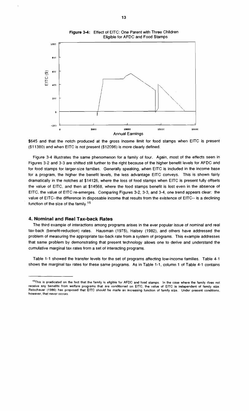
Flgure 3-4: Effect of EITC: One Parent with Three Children Eligible for AFDC and Food Stamps

I I -200

I d 0 so00 10000 lS000 20000

Annual Earnings

$645 and that the notch produced at the gross income limit for food stamps when ElTC is present ($1 1380) and when ElTC is not present ($12096) is more clearly defined.

Figure 3-4 illustrates the same phenomenon for a family of four. Again, most of the effects seen in Figures 3-2 and 3-3 are shifted still further to the right because of the higher benefit levels for AFDC and for food stamps for larger-size families. Generally speaking, when EITC is included in the income base for a program, the higher the benefit levels, the less advantage ElTC conveys. This is shown fairly dramatically in the notches at $14126, where the loss of food stamps when ElTC is present fully offsets the value of EITC, and then at $14568, where the food stamps benefit is lost even in the absence of EITC, the value of ElTC re-emerges. Comparing Figures 3-2, 3-3, and 3-4, one trend appears clear: the value of EITC--the difference in disposable income that results from the existence of EITC-- is a declining function of the size of the family.15

4. Nominal and Real Tax-back Rates The third example of interactions among programs arises in the ever popular issue of nominal and real

tax-back (benefit-reduction) rates. Hausman (1975), Halsey (1982), and others have addressed the problem of measuring the appropriate tax-back rate from a system of programs. This example addresses that same problem by demonstrating that present technology allows one to derive and understand the cumulative marginal tax rates from a set of interacting programs.

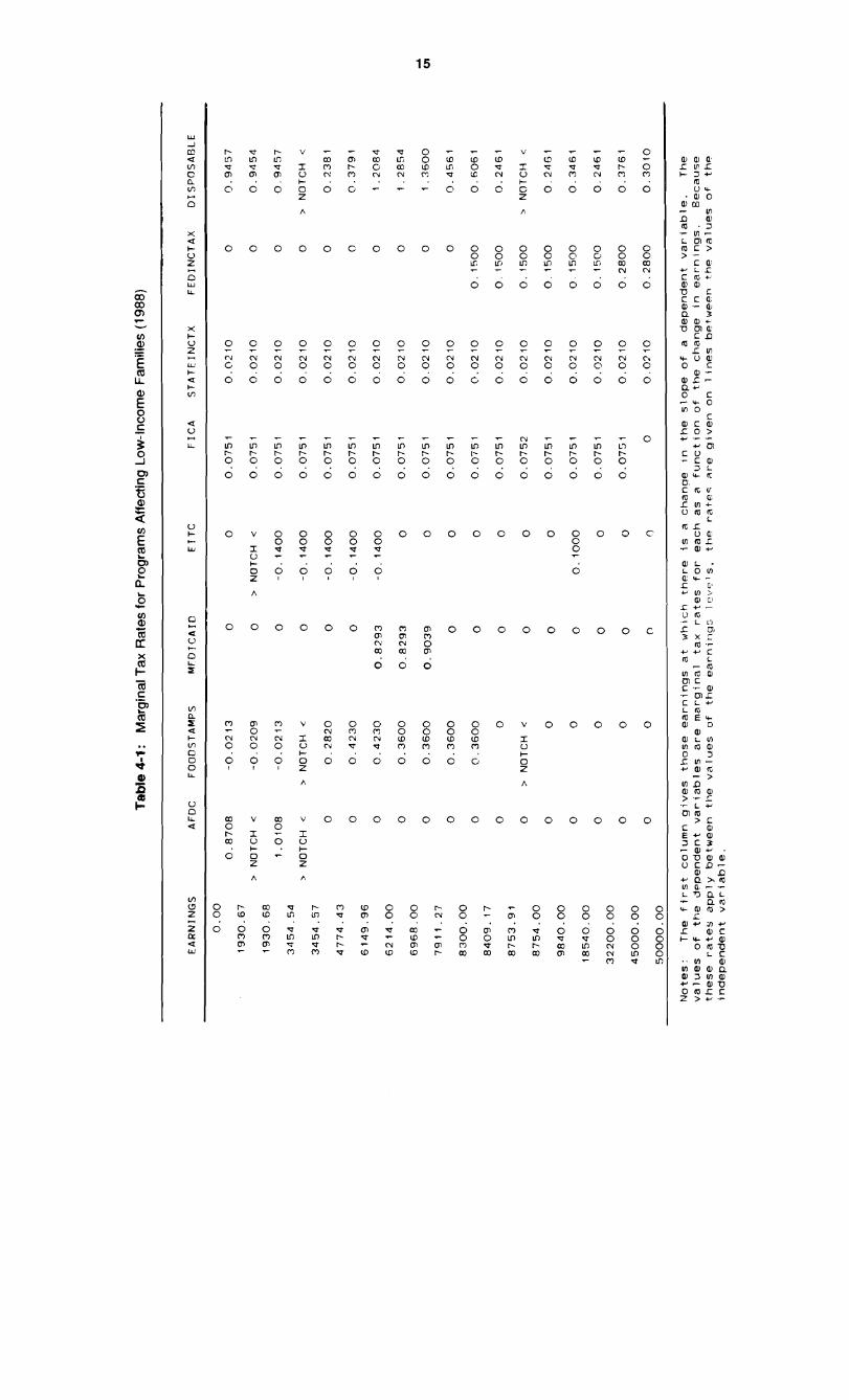
Table 1-1 showed the transfer levels for the set of programs affecting low-income families. Table 4-1 shows the marginal tax rates for these same programs. As in Table 1-1, column 1 of Table 4-1 contains

his is predicated on the fact that the family is eligible for AFDC and focd stamps. In the case where the family does not receive any benefits from welfare programs that are conditioned on EITC, the value of ElTC is independent of family size. Reischauer (1986) has proposed that ElTC should be made an increasing function of family size. Under present conditions, however, that never occurs.

values of the independent variable at which there is a change in the slope of a dependent variable. The values within the body of the table are the true marginal tax rates for each of the dependent variables as a function of the increase in the independent variable.

Between earnings of $0 and $1930.67, the marginal tax rate on AFDC is .8708, on food stamps -.0213, on Medicaid 0 (because in this range Medicaid is constant-valued at $1531), on ElTC 0 (because the family is not eligible for EITC), on FICA .0751, and on the state tax .021. Except for rounding error, the sum of these marginal tax rates equals the marginal tax rate for disposable income, .9457. When

earnings are $1930.67, they equal the amount from AFDC, the family then becomes eligible for EITC, and the AFDC benefit is accordingly adjusted. Between $1930.68 and $3454.54 the marginal tax rate remains the same for food stamps, FICA, and the state income tax, but for AFDC it increases by .14 to 1.0108, and the marginal tax rate for ElTC becomes -.14. At $6149 the medically needy Medicaid benefits begin to be reduced, with a marginal tax rate of .8293 in Medicaid, and a total marginal tax rate of 1.2084. When ElTC becomes constant at earnings of $6214, the marginal tax rate for food stamps declines to .36, and the total marginal tax rate is 1.2854. Between $6214 and $18540, the marginal tax rate on disposable income increases and decreases as benefits end and federal taxes begin. The marginal tax rate on disposable income also changes as a result of provisions and events within the welfare and taxation programs.16 At $18540, EITC, the last of the benefit programs included in this analysis, terminates, and the marginal tax rate on disposable income is .2461, a function solely of the various taxes.

Thus, at one level the goal of producing the decomposition of the total marginal tax rate into the individual components has been achieved. But the analyst may well want to pursue the matter further. What, for example, determines the specific marginal tax rates within AFDC?

The marginal tax-back rate in AFDC arises from the marginal tax rates for EITC, marginal changes in day care expenses (to the extent allowed in AFDC), marginal changes in work expenses (to the extent allowed in AFDC). and the marginal changes due to the earned income deduction in AFDC. As can be seen in Table 4-2, for income less than $1930.68, the marginal tax rate for ElTC is 0, since ElTC is not available. But the marginal tax rate for AFDC is also affected by day care expenses and work expenses. Because of the nature of our assumptions about work expenses, the work expense deduction has a marginal rate of change of ,1292 in this range of earnings. Therefore the marginal tax rate for AFDC is 1 minus .1292, or .8708. From $1930.68 to $3454.54, earnings together with ElTC would induce a marginal tax rate of 1 14O/0 in AFDC. Subtracting the .I292 marginal rate for the work expense deduction results in an AFDC marginal tax rate of 1.0108.

For each of the dependent variables one could examine the features of the programs and the programs on which the dependent variable is based that cause changes in the marginal tax rate. The previous example is probably sufficient, however, to demonstrate the point that it is fairly easy to obtain the true marginal tax rate for a program or a set of programs and also to decompose the marginal tax rate into the

'"he word "notch" occurs within Table 4-1 where there are discontinuities in the marginal tax rates. At earnings of $1930.67, for example, this one-parent, one-child family becomes eligible for EITC. This vertical shifl in ElTC creates a corresponding notch in AFDC, but since the two changes are completely offsetting no notch is created for disposable income. On the other hand, at earnings of $3454.54, the family loses its eligibility for AFDC which creates a notch not only in AFDC but also in food stamps and in disposable income. The notch in the marginal tax rate for food stamps at $8753.91 is caused by termination of food stamps because the family's income reaches the maximum. Just prior to that notch, the food stamp benefit has a marginal tax rate of 0 since the family is receiving a constant-valued benefit, $10 per month.

N N r. 2 g g E g ; g g E z g E z z g o O o . . . . . . . . . . . . . . . . . . O O O O O O O O O O G O O O O O O O

~ - .- n - L m a m c > > .-

c (I' 4- L C c a + (U a u !z c c a a .- aJ n 3 a a + v m c

c n m a

L m + U ( U 0 c

Y m C U - c a

3 L a '+ IT 0. C C U a (I' r n + u m a

OIL - L 0 m a ! + - K a' - 0 ;

a D C W - u m - L L? s 0 1

3 X T a .-

Y Y C m L - m m F j a m C C .- a .- m L C L Y L IO m E + a 0

a a L m I n m a 0 3 s m - r a a - > 1 : % a > .- c .r L 4-

m m > c ' E 4 - :

3 c 3 - a + . O D a a U S D -

I a n v a x m m a - . - L D ~ L .- n m - $ a >

Table 4-2: Components of AFDC Marginal Tax Rate

E A R N I N G S E I T C WORKEXPDEO A F D C

1930.67 > N O T C H < 0. 1292 > N O T C H <

1930.68 - 0 .1400 0 .1292 I .O f08

3454.54 -0. 1400 0 .1292 > N O T C H <

components on which it in turn depends. While we could do this for additional variables it would take us beyond the goals of this paper. We turn instead to a final example of program interaction.

5. Effects of Interactions by Level of Government So far in this series of analyses we have looked at the effect of a given program and characteristics of

that program on the operation of another single program (example one), we have looked at the effect of a program on the rest of the entire system (example two), and we have looked at the marginal tax rates created throughout the system (example three). This final example addresses a different type of interaction: the impact of interactions among programs on federal and state expenditures. In addition to looking at the impacts on the different parties (that is, families, the state government, and the federal government), the analysis illustrates simultaneous modeling of two different systems and the variation of significant parameters that affect both systems.

The problem involves the choice of private versus subsidized day care for a low-income family. One of the reasons that this is an interesting problem is that while day care expenses affect the family's disposable income directly, they also affect disposable income indirectly; they enter into the computation of AFDC, food stamps, and the federal tax credit for dependent care expenses, as can be seen in Figure 1-1 . As a consequence of these interactions, it is far from clear what the net effect of a given level of day care expenses will be.

In many states low-income families are eligible for subsidized day care, and under some circumstances free day care. While it might seem obvious that free day care would be financially preferred by the family, that is not always the case. Lewis (1983) showed that before 1981 families could be substantially better off by purchasing private (nonsubsidized) day care, even fairly expensive day care, than by accepting free day care: the fact that the day care expenses entered into each of the programs previously mentioned meant that under certain circumstances the family would receive all of its expenses back and would extend the range of earnings over which it was eligible for Medicaid. That analysis also showed that following the changes to AFDC introduced in the Omnibus Budget Reconciliation Act of 1981, the financial incentives for families, for the state, and for the federal government changed markedly. Here we return briefly to the impact of day care expenses, but in the context of 1988. Once again we use the same family type that we have been examining in the previous examples: the single parent with one child.

The subsidized day care program in Pennsylvania provides reduced-cost day care to families as a function of the income of the parent and the number of children in the family. Families with income less than $300 per year receive free day care; those with income greater than this pay from $260 per year to

$1040 per year depending on their income and the size of the family.17 For the first child in day care, the family pays a "full fee." Families with more than one child in day care pay reduced rates for additional children. Families that are receiving AFDC "must pay an amount equal to the maximum amount for which the parent ... may be reimbursed through hislher personal expense deduction for child care ..." (Pennsylvania DPW, 1988). Since AFDC allows expenses that are "reasonable and necessary" up to the limit of $160 per month per child, we assume that that is what is charged in the subsidized day care program. Further, if the family is also eligible for the earned income deduction within AFDC, the family is charged only the previously specified fee schedule. Finally, if the family income exceeds 9O0/0 of the intermediate standard of the Bureau of Labor Statistics, the family is not eligible for subsidized day care, in which case we assume that the family necessarily reverts to the private day care system.

Given the various interactions among these programs, what are the financial incentives for the family to use subsidized or private day care, and what are the financial consequences to the state and the federal government that result from the family's choice? To answer this we model the situation under the assumption that the family uses private day care and under the assumption that the family uses subsidized day care. Since most of these programs use earnings as a controlling variable, it is natural to select that as the independent variable for this analysis. le

Flgure 5-1 : Effect on the Family of Using Private Rather Than Subsidized Day Care

0 2000 4000 6000 oooo 10000 12000 14000 ~bnnr !

Annual Earnings

Figure 5-1 shows the difference in the financial outcomes to the family. The horizontal axis in Figure 5-1 is annual earnings for the family; the vertical axis is the difference in disposable income if the child is in a private day care center rather than a subsidized day care center. Positive values would mean that the family is better off financially with the child in private day care, and negative values mean that the family is better off financially with the child in subsidized day care.

Unlike the situation before 1981, the family is currently never better off financially if the child is in

he program defines fee schedules as a given amount per week depending on the gross income per month. We have translated all amounts into their annual equivalents.

"All four of the examples that we have introduced have used earned income as the independent variable, but that is not the only independent variable that one can use when building a MAPSIT-type model. Lewis and Morrison (1987) provide several examples of other types of independent variables, including "hours worked per week" and "proportion of income produced by the second earner in a two-earner household."

private day care, at least under the assumptions of this analysis. If the family's income is less than

$4749, there is no difference in financial outcome because the subsidized day care program charges the maximum that can be reimbursed through A F D C . ~ ~ Thus, whether the child is in the subsidized or the nonsubsidized day care program, the day care expense deduction that the family will be able to claim will be the same, and consequently the breakeven point for AFDC will be the same: $4749. For incomes

beyond this amount, however, there is a difference between the two outcomes. The principal difference is the cost of day care itself. At an income of $6968 (full time at the minimum wage) private day care for this family would cost $3325 and public day care $260. Because of its greater day care costs, the family choosing private day care would receive $1 503 in food stamps, and the family in public day care $756.20 The family using private day care would still be eligible for $1531 in medical coverage but the greater "available income" of the family in public day care would reduce the expected Medicaid benefit to $1 11 3, a difference of $418. Neither family would be eligible for the dependent care tax credit because neither family would be subject to any federal income tax. The total difference between the disposable incomes of these two families then is $1900. When the income for the family reaches $14,160 the family is no longer eligible for subsidized day care, and so there is once again no difference.

Between incomes of $4749 and $14,160 the advantage of subsidized day care varies from as little as $730 (for incomes between $831 4 and $8754) to as much as $2279 (at income of $1 1590). Some of the events that affect the magnitude of the advantage to public day care are the differential marginal tax rates in food stamps (as a function of the differential day care expenses), the differential magnitude of the tax credit (as a function of the day care expenses), the differential marginal tax rates in the MNO medical assistance program (as a result of differential day care expenses), and the differences in the day care expenses themselves. The notch at earnings of $8754 occurs because of the loss of food stamps at that level both for the family in private day care and for the family in subsidized day care. The food stamp benefit is terminated at this point because of the restriction on gross income.

In Figure 5-1 there are notches at $7872, $9444, $1 1016, and $12588 that are due to the fee schedule for subsidized day care. The one at $7872, before the food stamp benefit is terminated, has a minor but interesting effect. Since the full cost of day care is deductible in the medically needy Medicaid program, the increase of $104 is fully offset in Medicaid for the family in public day care. In addition, the family using public day care receives $47 more in food stamps because of the fee increase, leaving the family $47 better off because of the $104 increase in day care costs.21 The notches at $9444, $1 1016, and $12588 are more easily discerned and have effects that are intuitively more obvious: the notch produced by the increase in the day care fee in public day care increases the attractiveness of private day care, but the overall incentive is still to stay in the public day care system.

The choice of this problem, however, was driven by an interest in the effects on federal and state expenditures. Since the federal and state governments bear the costs of different portions of these programs, the impact of the choice of private or subsidized day care is borne differently by these two

'"here would be a difference, however, if AFDC terminated after the point at which the private day care expenses exceed the maximum allowable day care expense in AFDC.

"AS in the previous examples, we assume that ElTC is included as available income in the calculation of food stamp benefits.

"~edicaid has real value only if the family needs it. When medical expenses exist. the family is better off by virtue of its Medicaid eligibility: in the present case, if there were no medical expenses, the family would not be better off because of the increase in day care expenses.

levels of government. In this analysis we have assumed that the federal government bears 50% of the costs of AFDC and Medicaid, 75% of the costs of Title XX day care, and 100% of the costs of food stamps and the dependent care tax credit.

Figures 5-2 and 5-3 show the differential costs to the federal and state governments as a result of the family's choice. Again the results are a function of the income level of the family because the programs are individually (and jointly) conditioned on family income. Figure 5-2 shows that the federal government is as much as $1924 better off (at family earnings of $1 1590) i f the family were to pick private day care. This "benefit" to the federal government reflects a decrease in costs that would be incurred if the family uses private day care, even though the costs to the federal government from food stamps and dependent care tax expenditure would be greater i f the family were to choose private day care rather than subsidized day care. The low sloping portion bemeen earnings of $0 and $4749, where AFDC is eliminated, reflects the fact that when the family is in subsidized day care, even though it pays a fee equal to the private rate ($3325 for full-time day care), this is still less than the maximum rate at which subsidized day care providers can be reimbursed by the government. As a result, the federal and state governments share the portion of these day care costs that are not recaptured through the charge to families.

Figure 5-2: Effects on the Federal Level of Family Choice of Private Day Care over Subsidized Care

0 2000 4000 60t10 8000 10000 12000 14000 lC000

Annual Earnings

0 2000 400@ 600n 8000 10000 12000 14000 160~r!

Annual Earnings

Flgure 5-3: Effects on the State Level of Family Choice of Private Day Care over Subsidized Care

2000 C

C Q,

E

-

The magnitude of the differential in total costs is driven by the difference in the fee schedule for subsidized day care versus private day care, minus the reductions experienced from smaller outlays for food stamps, smaller reimbursements in MNO medical assistance, and smaller tax expenditures through the dependent care tax credit. The effects on the state are somewhat similar, though much reduced in magnitude, as is shown in Figure 5-3.

Since we have already introduced the fact that the subsidized day care program in the state takes into account whether or not the family is eligible for the earned income deduction within AFDC, we shall take advantage of the opportunity to show how relatively minor changes within programs can produce rather striking effects.

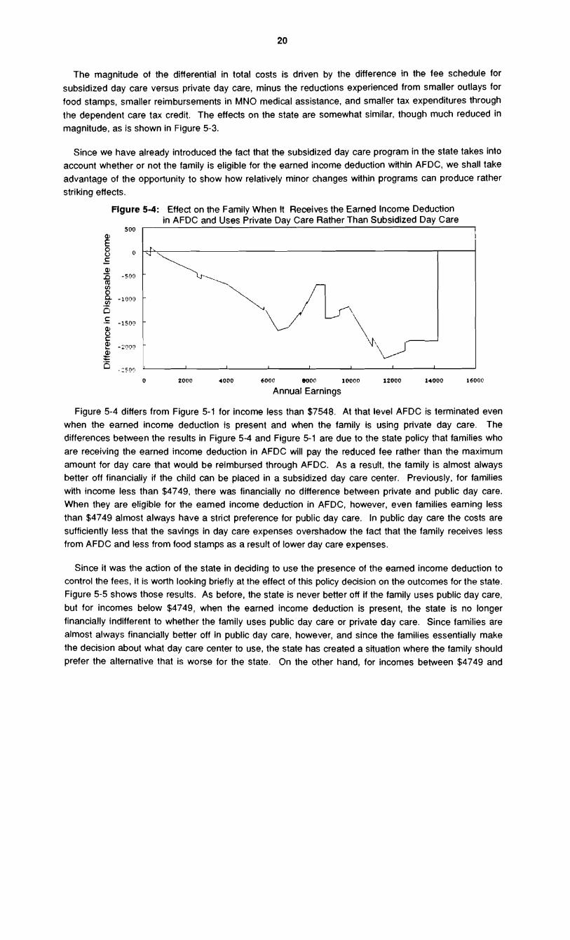
Flgure 5-4: Effect on the Family When It Receives the Earned Income Deduction in AFDC and Uses Private Day Care Rather Than Subsidized Day Care

0 2000 4000 6000 0000 10000 12000 14000 16000

Annual Earnings

Figure 5-4 differs from Figure 5-1 for income less than $7548. At that level AFDC is terminated even when the earned income deduction is present and when the family is using private day care. The differences between the results in Figure 5-4 and Figure 5-1 are due to the state policy that families who are receiving the earned income deduction in AFDC will pay the reduced fee rather than the maximum amount for day care that would be reimbursed through AFDC. As a result, the family is almost always better off financially if the child can be placed in a subsidized day care center. Previously, for families with income less than $4749, there was financially no difference between private and public day care. When they are eligible for the eamed income deduction in AFDC, however, even families earning less than $4749 almost always have a strict preference for public day care. In public day care the costs are sufficiently less that the savings in day care expenses overshadow the fact that the family receives less from AFDC and less from food stamps as a result of lower day care expenses.

Since it was the action of the state in deciding to use the presence of the eamed income deduction to control the fees, it is worth looking briefly at the effect of this policy decision on the outcomes for the state. Figure 5-5 shows those results. As before, the state is never better off if the family uses public day care, but for incomes below $4749, when the earned income deduction is present, the state is no longer

financially indifferent to whether the family uses public day care or private day care. Since families are almost always financially better off in public day care, however, and since the families essentially make the decision about what day care center to use, the state has created a situation where the family should prefer the alternative that is worse for the state. On the other hand, for incomes between $4749 and

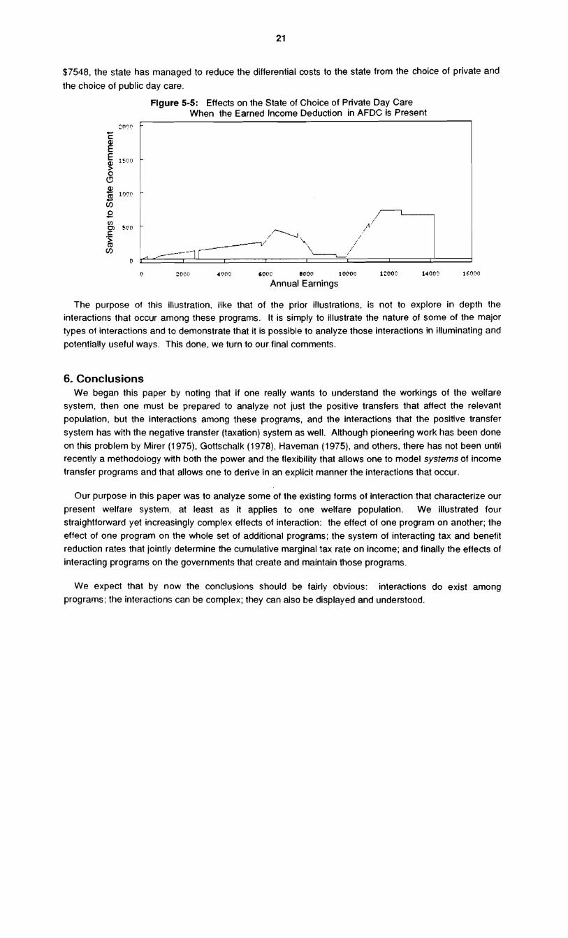
$7548, the state has managed to reduce the differential costs to the state from the choice of private and the choice of public day care.

Flgure 5-5: Effects on the State of Choice of Private Day Care When the Earned Income Deduction in AFDC is Present

r? *oc)c; 4000 6000 ~ 0 0 0 10000 1:oor 14r)oq l ~ n o n Annual Earnings

The purpose of this illustration, like that of the prior illustrations, is not to explore in depth the interactions that occur among these programs. It is simply to illustrate the nature of some of the major types of interactions and to demonstrate that it is possible to analyze those interactions in illuminating and potentially useful ways. This done, we turn to our final comments.

6. Conclusions We began this paper by noting that if one really wants to understand the workings of the welfare

system, then one must be prepared to analyze not just the positive transfers that affect the relevant population, but the interactions among these programs, and the interactions that the positive transfer system has with the negative transfer (taxation) system as well. Although pioneering work has been done on this problem by Mirer (1975), Gottschalk (1978), Haveman (1975), and others, there has not been until recently a methodology with both the power and the flexibility that allows one to model systems of income transfer programs and that allows one to derive in an explicit manner the interactions that occur.

Our purpose in this paper was to analyze some of the existing forms of interaction that characterize our present welfare system, at least as it applies to one welfare population. We illustrated four straightforward yet increasingly complex effects of interaction: the effect of one program on another; the effect of one program on the whole set of additional programs; the system of interacting tax and benefit reduction rates that jointly determine the cumulative marginal tax rate on income; and finally the effects of interacting programs on the governments that create and maintain those programs.

We expect that by now the conclusions should be fairly obvious: interactions do exist among programs; the interactions can be complex; they can also be displayed and understood.

Appendix: Assumptions and Program Representation The model includes three different welfare/social assistance programs (AFDC, food stamps, and

Medicaid), three taxes (FICA, federal income tax, and a state income tax), the dependent care tax credit, and the earned income tax credit. In calculating these transfers the model also generates a number of intervening variables, e.g., presumed child care expenses and shelter costs.

There are a number of special assumptions and characteristics in the model: The calculations apply to a single-parent family, but the model permits the analyst to specify any number of children.

The simulation employs a time period of one year. Programs administered on a shorter period are thus "scaled upn to annual equivalents.

The model assumes that the working parent receives wage and salary income at a constant rate throughout the year.

The analysis is limited for most purposes to families with gross earnings (wages and salaries) less than $20,000.

When a single parent is working, the family may be eligible for a tax credit for child care expenses. Section 8 of this appendix contains the specific assumptions about that credit.

The model asks whether the parent has been employed for more than 4 months and more than 12. The latter determines whether $30 is deducted from earnings each month; the former determines whether the 33% earnings' exemption applies.

The model assumes that all children are (a) under age 18 or (b) under age 19 and a full time student in secondary school or an equivalent level of a vocational or technical school.

The value of food stamps is treated as a cash benefit.

The value of the medical expenses reimbursed by Medicaid is treated as a cash benefit (see section 6).

The fixed parameters in the model employ numerical values appropriate for 1988.

1. Calculation of Transfers for Programs That Have No Other Programs as Inputs FICA contributions are calculated using 1988 parameters as 7.51% of earnings up to a maximum contribution of $3379.50, occurring at an earnings level of $45,000.

State income taxes are calculated as a fixed proportion (.021) times the quantity "total income (earnings plus other taxable income) less the allowable exemption."

2. Calculation of the Earned Income Tax Credit After defining the earned income tax credit schedule, the model computes the credit on two bases: (1)

using earnings as the income base, and (2) using adjusted gross income as the income base. It then selects (1) or (2) respectively as adjusted gross income is less than or greater than $9840. Finally, the credit is disallowed if there are no children in the family or if the child does not qualify as a dependent. The test for dependency is conducted by comparing income from AFDC with earnings and other taxable income. If more income is provided by AFDC than by earnings and other taxable income, the child is deemed not to be a dependent of the parent.

3. Child Care Expenses Since several programs (AFDC, food stamps, and the dependent care tax credit) use information about

child care expenses, a special section makes the initial calculations. The following assumptions are

relevant:

Day care use is proportional to work effort and that at $3.35/hr (minimum wage in January 1988) earnings of $6968 correspond to full-time employment. Income above $6968 is assumed to be the result of full-time employment at a higher wage rate.

Full-time day care expenses are assumed to be $3325 per child per year, based on a survey of day care centers in Pittsburgh in May 1980 and updated by an average of 5% per year for assumed increases in day care costs from 1980 to 1988.

The model assumes that day care is needed only i f the child is preschool age (age five or younger).

4. Calculation of AFDC Benefits The schedule of monthly maxima (as a function of family size) for Section 2 of Pennsylvania, January 1988, is converted to an annual basis. (Section 2 includes a majority of the counties in Pennsylvania and most of the metropolitan areas.)

Available income for calculating AFDC is equal to earnings plus ElTC and other taxable income, less deductions for work expenses, child care expenses, and the earned income exclusion, i f applicable. Since ElTC is not available to the family unless the nontransfer income is greater than the transfer income, AFDC is calculated separately without ElTC and "with" EITC. The appropriate value of AFDC is then chosen depending on the relation between AFDC and nontransfer income.

The work expense deduction is $75 per month, prorated for less than full-time work. (This method of operationalizing work expenses has a direct effect on marginal tax rates for incomes below full-time employment.)

Child care expenses are deductible if necessary to work, with a maximum deduction per child per month of $160. We shall assume that day care is allowed proportional to hours worked up to a maximum of 40 hours per week. (This method of operationalizing day care expenses has a direct effect on marginal tax rates for incomes below full-time employment.)

The earned income exclusion is $30 per month if it has been received for less than 12 months; the earned income exemption is one-third of the net earned income (net earned income is earned income minus the deductions for work expenses, child care expenses and the first $30 per month), but this exclusion is not allowed after the first four months.

Benefits payable to the family are equal to the guarantee less available income, subject of course to the condition that the benefit not be negative.

Finally, if the available income (earnings, EITC, and other income) is greater than 185% of the need standard, the family is ineligible for any AFDC benefit.

5. Calculation of Food Stamp Benefits This calculation is divided into two parts. Section 5.1 derives the income base as a function of

earnings; section 5.2 derives the nominal benefit schedule and actual food stamp benefits as a function of the food stamp income base.

5.1. Derlvatlon of the Income Base for Food Stamps "Net food stamp income" is calculated as the sum of earned income, unearned income (including in the latter category aid from federal or federally aided public assistance programs, e.g., SSI and AFDC), and the earned income tax credit (EITC), and less a series of deductions:

a standard deduction, $1224 per year ($102 per mo.)

an earned income deduction, 20% of earned income

a dependent care deduction

a deduction for medical costs in excess of $35 a month (for persons age 60 or over)

an excess shelter costs deduction.

The maximum dependent care deduction is $1920 per year ($160 per month) or actual expenses whichever is less. We assume that the actual expenses are equal to the child care expenses previously defined in this model and that there are no other dependent care expenses. *

Excess shelter costs are defined as shelter costs in excess of 50% of the net income (income after the standard deduction, the earned income deduction, the dependent care deduction, and the medical expense deduction). These excess expenses are deductible up to a maximum of $1 968 per year ($164 per month).

5.2. Derlvatlon of Food Stamp Benefit The maximum monthly bonus value by family size is selected and converted to an annual amount.

We derive the preliminary nominal schedule for food stamp benefits by applying a 30% reduction rate (with respect to the food stamp income base) on the maximum bonus for the family and by imposing a $10 per month ($120/year) minimum on benefits payable.

We obtain the maximum net and gross incomes per year and use these to control the termination of food stamp benefits.

Current rules require that the unit meet both net and gross income limits unless the unit is categorically eligible (e.g., by being AFDC or SSI eligible).

If the unit is categorically eligible the benefit is still calculated using the food stamp income base, but the unit continues to receive at least $10 per month as long as it is categorically eligible.

6. Calculation of Medicaid Benefits For earnings levels at which the family receives a positive benefit from AFDC, Medicaid is assumed to reimburse the family's medical expenses; otherwise the family is assumed to pay the medical expenses itself.

To determine the value of medical benefits we use the Census Bureau's per person nationwide dollar estimates for noninstitutionalized persons: $851 per adult recipient and $417 per child (both per year). (Bureau of the Census, 1985)

These values for 1984 are updated to 1988 by the average rate of increase in Medicaid outlays between 1981 and 1986: 3.6% per year for adults and 7.2% per year for children. The 1988 values are thus $980 per adult and $551 per child.

Families are categorically eligible for Medicaid if they receive a payment from AFDC or if they would have received a payment except for the $1 0 minimum payment regulation in AFDC.

Families not categorically eligible for Medicaid may still be eligible for the "medically needy only" program. The first step in determining eligibility is to compute net available income. In Pennsylvania at present this includes earnings, minus deductions, plus unearned income. The deductions include "personal expenses" (transportation to and from work, and day care expenses necessary for work) and "work expenses" (federal income tax withholding, state income tax withholding, FICA, local wage tax withholding, and union dues). The net income is then compared to the medically needy income limitation, which is a function of family size. If the net income is less than the income limitation, the medical expenses will be covered, provided that the family also meets the resource limitations test. If the net income is more than the medically needy income limitation, the difference is deemed available to pay medical expenses and the medically needy program will pay only the remainder. This produces essentially a dollar for dollar reduction of the net income in excess of the income limitation.

7. Calculation of Federal Income Tax The tax calculation uses Schedule Z, even though low-income filers would normally use the tax tables.

Schedule Z is used because there is a single-parent family.

Taxable income is calculated as total income less $1950 per person (which in 1988 is reduced for higher incomes) and less the standard deduction of $4400 for head of household filers.

8. Tax Credit for Child Care Expenses The dependent care tax credit is computed under the following assumptions:

Since there is only a single parent the conditions related to two-parent families can be ignored.

We assume there are no disabled dependents and limit relevant expenses to those for preschool children in a day care facility.

Although the child care credit is available when a parent is not working but is looking for a job, we have ignored this provision and assumed that the parent receives credit only for the portion of time that child care was required for actual employment.

The test of whether the parent has supplied more than 50% of the cost of running a home is approximated by testing whether the parent's total income (before transfers) is equal to or greater than the transfers, in this case AFDC.

Maximum allowable dependent care expenses are $2400 if there is only one dependent and $4800 if there are two or more dependents, but the maximum allowable expenses can never be greater than the actual expenses or greater than earned income.

The credit is derived as a variable percentage (30% if earnings are less than $1 0000, to 20% if earnings are greater than $28000) of the maximum allowable dependent care expenses, but never more than the federal taxes to be paid. Rather than use the entire set of step functions employed by the IRS, we have modeled the reduction in the percentage as a "half-step" step function at $10000 and a "half-step" step function at $28000, with a linear decrease between these two points.

The maximum credit, then, is $720 for one dependent and $1440 for two or more dependents.

9. Disposable Income Different analysts use different definitions of disposable income. The one we employ includes all

income sources for the family (earnings, other taxable income, and all program benefits) and then deducts involuntary outflows (FICA premiums, state income taxes, and federal income taxes). In addition, it treats food stamps and Medicaid as if they were cash benefits.

References

Bureau of the Census. (1985) Estimates of Poverty including the Value of Noncash Benefits--1984, Technical Paper 55. (Washington, D.C.: U.S. Government Printing Office), pp. 53-66.

Committee on Ways and Means, U.S. House of Representatives. (1985) "Background Material and Data on Programs within the Jurisdiction of the Committee on Ways and Means." (Washington, D.C.: U.S. Government Printing Office, February 22).

Domestic Policy Council: Low lncome Opportunity Working Group. (1 986) Up From Dependency: A New National Public Assistance Strategy. December.

Gottschalk, Peter. (1 978) "Principles of Tax Transfer Integration and Carter's Welfare Reform Proposal," Journal of Human Resources, 1 3(3):332-348.

Halsey, Harlan. (1 982) "The Taxation of Transfer Income," Journal of Human Resources, 17(4):558-580.

Hausman, Leonard. (1975) "Cumulative Tax Rates in Alternative lncome Maintenance Systems," in I. Lurie (ed.), lntegrating lncome Maintenance Programs, (New York: Academic Press).

Haveman, Robert. (1 975) "Earnings Supplementation as an lncome Maintenance Strategy: Issues of Program Structure and Integration," in I. Lurie (ed.), lntegrating lncome Maintenance Programs, (New York: Academic Press).

Joint Committee on Taxation. (1987) General Explanation of the Tax Reform Act of 1986: H.R. 3838, 99th Congress; Public Law 99-514 (Washington, D.C.: U. S. Government Printing Office, May 4).

Lewis, Gordon H. (1983) "The Daycare Tangle: Unexpected Outcomes When Programs Interact," Journal of Policy Analysis and Management, 2(4):531-547.

Lewis, Gordon H., and Richard J. Morrison. (1983) "Coordinating lncome Transfer Programs," Policy and Information, 7(1):93-124.

Lewis, Gordon H., and Richard J. Morrison. (1987) lncome Transfer Analysis (New York: lmmergut & Siolek).

Mirer, Thad. (1975) "Alternative Approaches to lntegrating lncome Transfer Programs," in I. Lurie (ed.), lntegrating lncome Maintenance Programs (New York: Academic Press).

Morrison, Richard J., William Bradley, et al. (1985) MAPSIT: Modular Analysis Package for Systems of lncome Transfer, Version 5 (Ottawa, Canada: Department of National Health and Welfare, Policy, Planning, and Information Branch, Technical Report).

Pennsylvania Department of Public Welfare. (1988) Title 55: Public Welfare; Part V.: Children, Youth and Families Manual; Chapter 3040: Subsidized Child Day Care (Harrisburg, Pa.: PDPW)

Reischauer, Robert D. (1986) "It Can Help the Poor Even More," Washington Post, June 1, p. C8.

Steuerle, Eugene, and Paul Wilson. (1987) "The Earned lncome Tax Credit," Focus, 10(1):1-8 (Newsletter of the Institute for Research on Poverty, University of Wisconsin, Madison).

Storey, James R. (1972) "Public lncome Transfer Programs: The Incidence of Multiple Benefits and the Issues Raised by Their Receipt," In Subcommittee on Fiscal Policy, Joint Economic Committee, U.S. Congress, Studies in Public Welfare (Washington, D.C.: U.S. Government Printing Office).