unsaturated soils and foundation design: theoretical
TRANSCRIPT

Unsaturated Soils and Foundation
Design: Theoretical Considerations
for an Effective Stress Framework
AN ABSTRACT OF THE THESIS OF
Josiah D. Baker for the degree of Master of Science in Civil Engineering presented on
June 2, 2016.
Title: Unsaturated Soils and Foundation Design: Theoretical Considerations for an Ef-
fective Stress Framework
Abstract approved:
T. Matthew Evans
This study presents the theoretical background necessary to model the bearing capacity
of shallow and deep foundations in partially saturated soils. The conventional bearing
capacity equations for shallow and deep foundations and the 𝛽-method for deep foun-
dation side resistance have been modified to include the effects of matric suction and
varying water contents according to the effective stress framework. A closed-form so-
lution has been proposed for the bearing capacity equation that modifies the overbur-
den, unit weight, and cohesion terms in the conventional equation. The 𝛽-method has
been modified to consider suction stresses along the deep foundation and a reduction
in K0 due to tension cracking near the surface. The modified bearing capacity equation
for shallow foundations shows good agreement to load-tests performed in partially sat-
urated soils. Monte Carlo simulations were performed on silt loams, sands, and clays
to characterize variance and distribution of bearing capacity. The results show that silts
have the largest variance while clays have the smallest variance in predicted bearing
capacity.

© Copyright by Josiah D. Baker
June 2, 2016
All Rights Reserved

Unsaturated Soils and Foundation Design: Theoretical Considerations for an
Effective Stress Framework
by
Josiah D. Baker
A THESIS
submitted to
Oregon State University
in partial fulfillment of
the requirements for the
degree of
Master of Science
Presented June 2, 2016
Commencement June 2017
Master of Science thesis of Josiah D. Baker presented on June 2, 2016.
APPROVED:
Major Professor, representing Civil Engineering
Head of the School of Civil and Construction Engineering
Dean of the Graduate School
I understand that my thesis will become part of the permanent collection of Oregon
State University libraries. My signature below authorizes release of my thesis to any
reader upon request.
Josiah D. Baker, Author

ACKNOWLEDGEMENTS
First, I would like to thank my advisor, Professor Matt Evans, for his dedication, support, and
insight in writing this thesis. During my undergraduate, his passion for geotechnical engineer-
ing spurred within me an interest to pursue this discipline. Since then, he has been instrumental
in the completion of my education and research both during my undergraduate and graduate
studies at Oregon State University.
I would also like to give my sincerest appreciation to my friends at Grant Avenue Baptist
Church for their continual love, making my time at Oregon State University a memorable ex-
perience. They have encouraged me to grow in my faith as a Christian.
I am grateful to my parents and siblings for their patience and love throughout college. They
helped me through all my life decisions. I could not find a more supportive family than this.
Finally, I would like to thank my fiancé Rebecca. She has been a wonderful friend, challenging
me each day to pursue excellence while still encouraging me to enjoy life’s important moments.

TABLE OF CONTENTS
Page
1. Introduction ............................................................................................................1
1.1. Statement of Problem ......................................................................................1
1.2. Purpose and Scope ..........................................................................................1
1.3. Outline .............................................................................................................1
1.4. Qualifications and Limitations ........................................................................2
2. Background ............................................................................................................3
2.1. Shallow Foundations .......................................................................................3
2.1.1. General Bearing Capacity Theory for Shallow Foundations ...................3
2.1.2. Various Improvements on Bearing Capacity Equation ...........................8
2.1.3. Recent Developments ............................................................................11
2.2. Deep Foundations .........................................................................................13
2.2.1. Analytical Theory ..................................................................................13
2.2.2. Recent Developments ............................................................................18
2.3. Mechanics of Unsaturated Soils ....................................................................19
2.3.1. Soil Water Characteristic Curve ............................................................19
2.3.2. Particle Level Principles ........................................................................20
2.3.3. Bishop’s Effective Stress Framework ...................................................23
2.3.4. Solutions for Bishop’s Effective Stress Parameter ................................24
2.3.5. Extended Mohr-Coulomb Failure Criterion ..........................................26
2.3.6. Matric Suction Profiles ..........................................................................27
2.3.7. At-Rest Earth Pressure Coefficient ........................................................29
2.3.8. Discussion of Unsaturated Soil Properties ............................................30
2.4. Summary .......................................................................................................32
3. Research Objectives and Methodology ...............................................................35

TABLE OF CONTENTS (CONTINUED)
Page
3.1. Objectives ......................................................................................................35
3.2. Shallow Foundations in Unsaturated Soils ...................................................37
3.2.1. Theoretical Development .......................................................................37
3.2.2. Considerations for Apparent Cohesion ..................................................42
3.2.3. Considerations for Unit Weight .............................................................44
3.2.4. Considerations for Overburden ..............................................................46
3.3. Deep Foundations in Unsaturated Soils ........................................................47
3.3.1. Theoretical Development .......................................................................47
3.3.2. Tension Cracking and K0 .......................................................................50
3.3.3. Unit Weight ...........................................................................................52
3.3.4. Suction Stresses .....................................................................................52
3.4. Summary .......................................................................................................53
4. Comparison to Measured Response of Shallow Foundations..............................54
4.1. Introduction ...................................................................................................54
4.2. Method for the Selection of Load Test Data .................................................54
4.3. Comparison of Predicted Bearing Capacity to Database ..............................56
4.3.1. Steensen-Bach et al. (1987) ...................................................................56
4.3.2. Briaud and Gibbens (1997) ....................................................................60
4.3.3. Larsson (1997) .......................................................................................65
4.3.4. Viana da Fonseca and Sousa (2002) ......................................................69
4.3.5. Rojas et al. (2007) ..................................................................................71
4.3.6. Vanapalli and Mohamed (2007) / Oh and Vanapalli (2008) .................75
4.3.7. Vanapalli and Mohamed (2013) ............................................................80
4.3.8. Wuttke et al. (2013) ...............................................................................84

TABLE OF CONTENTS (CONTINUED)
Page
4.4. Summary and Discussion ..............................................................................88
5. Parametric Studies ...............................................................................................90
5.1. Outline of Parametric Studies .......................................................................90
5.2. Soils Parameters Used in Parametric Study ..................................................90
5.3. Parametric Studies on Shallow Foundations .................................................93
5.3.1. Shallow Foundation Bearing Capacity Profiles .....................................93
5.3.2. Evaluation of van Genuchten’s 𝛼 and 𝑛 ..............................................103
5.3.3. Other Considerations for Shallow Foundation Bearing Capacity .......108
5.3.4. Vahedifard and Robinson (2015) .........................................................116
5.4. Parametric Study on the Modified 𝛽-method .............................................124
5.4.1. Development of Side Resistance Profiles ............................................124
5.4.2. Evaluation of Side Resistance Profiles ................................................129
5.5. Monte Carlo Simulations for Partially Saturated Soils ...............................145
5.5.1. Silt Loam Analysis ..............................................................................146
5.5.2. Sand Analysis ......................................................................................151
5.5.3. Clay Analysis .......................................................................................154
5.6. Discussion ...................................................................................................157
6. Conclusions and Future Work ...........................................................................160
6.1. Conclusions .................................................................................................160
6.2. Implications for Geotechnical Engineering Practice ..................................161
6.3. Future Work ................................................................................................162
References ..................................................................................................................165
LIST OF FIGURES
Figure Page
Figure 2-1. Definitions of ultimate bearing capacity (from Terzaghi 1943) .................4
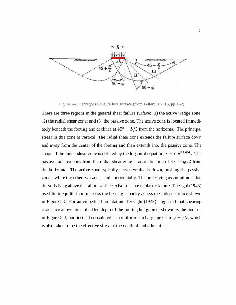
Figure 2-2. Terzaghi (1943) failure surface (from Fellenius 2015, pp. 6-2) .................5
Figure 2-3. General shear failure for embedded shallow foundation (from Vesić
1973) ...........................................................................................................................6
Figure 2-4. (a) General, (b) local, and (c) punching shear failure (Vesić 1973) ...........6
Figure 2-5. Comparison of different Nγ factors. (Left: lin-lin ordinate, Right:
lin-log ordinate) ........................................................................................................10
Figure 2-6. (a) Water content vs. matric suction. (b) two grains in contact with
water between contacts. ............................................................................................21
Figure 2-7. Forces acting on an individual particle (after Lu and Likos 2004). ..........22
Figure 2-8. (a) SWCC for sand, silt and clays, (b) corresponding suction stress
profile (Lu et al. 2010) ..............................................................................................26
Figure 2-9. Matric suction profiles at various surface flux boundary conditions
for clay (Lu and Griffiths 2004). ...............................................................................28
Figure 3-1. Soil water characteristic curve for this example soil. ..............................40
Figure 3-2. Suction stress profile for this example soil. ..............................................41
Figure 3-3. Failure surface corresponding to ϕ' = 20°, B = 2 m, and D = 0.5 m. ........42
Figure 3-4. Saturation of the soil profile for the example. ...........................................43
Figure 3-5. Failure surface of the shallow foundation, colored by the saturation
profile. .......................................................................................................................43
Figure 3-6. Sketch of the conceptual deep foundation considered in this work. .........48
Figure 3-7. Variation of At-Rest earth pressure coefficient in partially saturated
soils. ..........................................................................................................................51
Figure 4-1. SWCC for Sollerod sand (Steensen-Bach et al. 1987). .............................56
Figure 4-2. Load displacement curves for Sollerod sand with varying
groundwater tables ....................................................................................................58
LIST OF FIGURES (CONTINUED)
Figure Page
Figure 4-3. Measured bearing capacity vs. calculated bearing capacity for
Steensen-Bach et al. (1987) ......................................................................................59
Figure 4-4. Calculated bearing capacity vs. GWT depth for Steensen-Bach et
al. (1987) ...................................................................................................................60
Figure 4-5. Load displacement curve from Briaud and Gibbens (1997) .....................62
Figure 4-6. Comparison of measured bearing capacity to the conventional and
modified approach for Briaud and Gibbens (1997) ..................................................63
Figure 4-7. Comparison of measured bearing capacity with respect to footing
width (B) plus embedded depth (D) for Briaud and Gibbens (1997) .......................64
Figure 4-8. Predicted bearing capacity with respect to footing with using the
modified approach for the soil data provided by Briaud and Gibbens (1997)..........65
Figure 4-9. Hyperbolic fits to load displacement curve at Vatthammar site
(Larsson 1997) ..........................................................................................................67
Figure 4-10. Fitted hyperbolic load displacement curve for Viana da Fonseca
and Sousa (2002) data ...............................................................................................70
Figure 4-11. Fitted SWCC for the Rojas et al. (2007) data. ........................................73
Figure 4-12. Linearly interpolated matric suction profile for Rojas et al. (2007)
data ............................................................................................................................74
Figure 4-13. Comparison of calculated qult for the Rojas et al. (2007) data using
the modified and unmodified bearing capacity equation. .........................................74
Figure 4-14. Fitted SWCC using van Genuchten (1980) (after Vanapalli and
Mohamed 2007) ........................................................................................................77
Figure 4-15. Comparison of actual bearing capacity to predictions from this
work and Vanapalli and Mohamed (2007) ...............................................................78
Figure 4-16. Bearing capacity vs. variation in average matric suction from this
work and Vanapalli and Mohamed (2007) ...............................................................79
Figure 4-17. Comparison of measured and predicted bearing capacity for 150
mm surface plate for Vanapalli and Mohamed (2013) .............................................80
LIST OF FIGURES (CONTINUED)
Figure Page
Figure 4-18. Bearing capacity vs. variation in average matric suction from this
work and Vanapalli and Mohamed (2013) for a 150×150 mm plate loaded on
the surface. ................................................................................................................81
Figure 4-19. SWCC and suction stress profile for Vanapalli and Mohamed
(2013) soil. ................................................................................................................82
Figure 4-20. Comparison of measured and calculated bearing capacity for 150
mm embedded plate for Vanapalli and Mohamed (2013) ........................................83
Figure 4-21. Bearing capacity vs. variation in average matric suction from this
work and Vanapalli and Mohamed (2013) for a 150×150 mm plate embedded
150 mm. ....................................................................................................................84
Figure 4-22. Soil water characteristic curve for Hostun sand (after Wuttke et al.
2013) .........................................................................................................................86
Figure 4-23. Calculated and measured bearing capacities compared to the
average matric suction at D and D + B. ....................................................................87
Figure 4-24. Comparison of actual bearing capacity to predictions from the
conventional and modified approach for Wuttke et al. (2013) .................................88
Figure 4-25. Measured bearing capacity vs. predicted bearing capacity for
database of load tests in Chapter 4. ...........................................................................89
Figure 5-1. (a) Soil water characteristic curves for the 12 USDA Textural
Classes using van Genuchten parameters from Carsel and Parrish (1988).
Curves for sand, clay and silt loam are highlighted. (b) USDA Textural
Triangle (USDA 2016). ............................................................................................92
Figure 5-2. Shallow foundation bearing capacity profile of clay, silt, and sand
at varying friction angles. Note changing ordinate across figures. ...........................94
Figure 5-3. Shallow foundation bearing capacity vs. zgwt - D for clay, silt, and
sand at varying depths of embedment. Note changing ordinate across figures.
...................................................................................................................................95
Figure 5-4. Shallow foundation bearing capacity vs. groundwater table depth
for clay, silt, and sand at varying depths of embedment. Note changing
ordinate across figures. .............................................................................................96
Figure 5-5. Shallow foundation bearing capacity profile of clay, silt, and sand
with varying rates of flux. Note changing ordinate across figures. ..........................97
LIST OF FIGURES (CONTINUED)
Figure Page
Figure 5-6. Shallow foundation bearing capacity profile of clay, silt, and sand
with varying θs. Note changing ordinate across figures............................................99
Figure 5-7. Shallow foundation bearing capacity profile of clay, silt, and sand
with varying θr. Note changing ordinate across figures..........................................100
Figure 5-8. Shallow foundation bearing capacity profile with varying α. .................101
Figure 5-9. Shallow foundation bearing capacity profile with varying n. Note
changing ordinate across figures. ............................................................................102
Figure 5-10. Varying van Genuchten’s α at various ground table depths for n =
1.1............................................................................................................................104
Figure 5-11. Varying van Genuchten’s α at various ground table depths for n =
1.5............................................................................................................................104
Figure 5-12. Varying van Genuchten’s α at various ground table depths for n =
3.0............................................................................................................................105
Figure 5-13. Varying van Genuchten’s n at various ground table depths for 𝛼 =
0.01 kPa-1. ...............................................................................................................106
Figure 5-14. Varying van Genuchten’s n at various ground table depths for 𝛼 =
0.1 kPa-1. .................................................................................................................106
Figure 5-15. Varying van Genuchten’s n at various ground table depths for 𝛼 =
1 kPa-1. ....................................................................................................................107
Figure 5-16. Comparison of the predicted bearing capacity for a sand using the
modified and conventional approach at various friction angles, D = 0 m. .............109
Figure 5-17. Comparison of the predicted bearing capacity for a sand using the
modified and conventional approach at various friction angles, D = 1.5 m. ..........110
Figure 5-18. Comparison of the predicted bearing capacity between the
modified and conventional approach at various friction angles for a material
with D = 0 m, n = 3, and α = 0.1 kPa-1. ...................................................................111
Figure 5-19. Comparison of the predicted bearing capacity between the
modified and conventional approach at various friction angles for a material
with D = 1.5 m, n = 3, and α = 0.1 kPa-1. ................................................................111

LIST OF FIGURES (CONTINUED)
Figure Page
Figure 5-20. Comparison of the predicted bearing capacity for silt while varying
the footing width. This soil has zw = 4 m, 𝜙′ = 30˚ and D = 0.5 m. .......................112
Figure 5-21. Table of figures for qmod/qunmod. The x and y axis of the table
correspond to various ϕ' and zw/B ratios respectively. For each individual
figure, x and y axes are αzwγw and n, respectively. ..................................................114
Figure 5-22. Normailzation of the soil water characteristic curve.............................115
Figure 5-23. Calculated bearing capacity for hypothetical clay with D = 0 m
from Vahedifard and Robinson (2015) compared to modified approach in this
current work (left 𝜙′ = 25°, right 𝜙′ = 20°). .........................................................119
Figure 5-24. Calculated bearing capacity for hypothetical clay with D = 1.5 m
from Vahedifard and Robinson 2015 compared to modified approach in this
current work (left 𝜙′ = 25°, right 𝜙′ = 20°). Note changing ordinate across
figures. ....................................................................................................................119
Figure 5-25. Calculated bearing capacity for hypothetical sand with D = 0 from
Vahedifard and Robinson 2015 compared to modified approach in this current
work. .......................................................................................................................121
Figure 5-26. Calculated bearing capacity for hypothetical sand with D = 1.5 m
from Vahedifard and Robinson (2015) compared to modified approach in this
current work. ...........................................................................................................121
Figure 5-27. Comparison of calculated bearing capacity profiles using the
proposed approach, the Vesić solution, and Vahedifard and Robinson (2015)
for a surface foundation (left: 𝜙′ = 35° × 1.1, right: 𝜙′ = 30° × 1.1). .................122
Figure 5-28. Comparison of calculated bearing capacity profiles using the
proposed approach, the Vesić solution, and Vahedifard and Robinson (2015)
for an embedded foundation (left: 𝜙′ = 35°, right: 𝜙′ = 30°). ..............................123
Figure 5-29. Suction stress profile above the groundwater table for theoretical
sand, silt, and clay (θs = 0.4, θr = 0.06, q = 0 m/s for each figure). Note
changing abscissa across figures. ............................................................................125
Figure 5-30. Vertical effective stress as a function of depth from soil surface for
theoretical sand, silt, and clay (θs = 0.4, θr = 0.06, q = 0 m/s, Gs = 2.65 for
each figure). ............................................................................................................126
LIST OF FIGURES (CONTINUED)
Figure Page
Figure 5-31. Modified β’ as a function of depth from soil surface for theoretical
sand, silt, and clay (θs = 0.4, θr = 0.06, q = 0 m/s, Gs = 2.65, ν = 0.3, δ = 30˚
for each figure). .......................................................................................................127
Figure 5-32. Side resistance as a function of depth from soil surface for
theoretical sand, silt, and clay (θs = 0.4, θr = 0.06, q = 0 m/s for each figure). ......128
Figure 5-33. Side resistance profiles for theoretical sand, silt and clay (𝜈 = 0.3,
𝐺𝑠 = 2.65, 𝜃𝑟 = 0.06, and 𝜃𝑠 = 0.4) (unit side resistance given in force/unit
perimeter) ................................................................................................................130
Figure 5-34. Side resistance profiles for theoretical silt with varying specific
gravity (𝑛 = 1.5, 𝛼 = 0.1 kPa-1, 𝜈 = 0.3, 𝜃𝑟 = 0.06, and 𝜃𝑠 = 0.4) (unit side
resistance given in force/unit perimeter) .................................................................131
Figure 5-35. Side resistance profiles for theoretical silt with varying residual
water content (𝑛 = 1.5, 𝛼 = 0.1 kPa-1, 𝜈 = 0.3, 𝐺𝑠 = 2.65, and 𝜃𝑠 = 0.4) (unit
side resistance given in force/unit perimeter) .........................................................132
Figure 5-36. Side resistance profiles for theoretical silt with varying saturated
water content (𝑛 = 1.5, 𝛼 = 0.1 kPa-1, 𝜈 = 0.3, 𝐺𝑠 = 2.65, and 𝜃𝑟 = 0.06) (unit
side resistance given in force/unit perimeter) .........................................................133
Figure 5-37. Suction stress profiles of theoretical clay for flowrates of q = -
0.2ks, 0, and 0.2ks. ...................................................................................................134
Figure 5-38. Side resistance profiles of theoretical clay for flowrates of q = -
0.2ks, 0, and 0.2ks (𝑛 = 1.5, 𝛼 = 0.1 kPa-1, 𝜈 = 0.3, 𝐺𝑠 = 2.65, and 𝜃𝑟 = 0.06)
(unit side resistance given in force/unit perimeter) .................................................135
Figure 5-39. Suction stress profiles of theoretical silt for flowrates of q = -0.2ks,
0, and 0.2ks. .............................................................................................................136
Figure 5-40. Side resistance profiles of theoretical silt for flowrates of q = -
0.2ks, 0, and 0.2ks (𝑛 = 1.5, 𝛼 = 0.1 kPa-1, 𝜈 = 0.3, 𝐺𝑠 = 2.65, and 𝜃𝑟 = 0.06)
(unit side resistance given in force/ unit perimeter) ................................................137
Figure 5-41. Side resistance profiles for 𝜈 = 0.2 at various 𝑛 and 𝛼 values. ............138
Figure 5-42. Side resistance profiles for 𝜈 = 0.3 at various 𝑛 and 𝛼 values. ............139
Figure 5-43. Side resistance profiles for 𝜈 = 0.4 at various 𝑛 and 𝛼 values. ............140
LIST OF FIGURES (CONTINUED)
Figure Page
Figure 5-44. K0 as a function of depth from soil surface for α = 0.01 kPa-1, and
n = 3.0 for fixed groundwater table depths (θs = 0.4, θr = 0.06, q = 0 m/s, Gs
= 2.65, ν = 0.2, δ = 30˚) ..........................................................................................141
Figure 5-45. Unit weight profile for theoretical clay (θs = 0.4, θr = 0.06, q = 0
m/s, Gs = 2.65, α = 0.01 kPa-1, n = 1.1) ..................................................................143
Figure 5-46. Side resistance profiles of theoretical clay for 𝜈 = 0.2, 0.3, and 0.4
(𝑛 = 1.1, 𝛼 = 0.01 kPa-1, 𝐺𝑠 = 2.65, 𝜃𝑠 = 0.4 and 𝜃𝑟 = 0.06). Note changing
abscissa across figures. ...........................................................................................144
Figure 5-47. Probability histogram of silt loam properties from Carsel and
Parrish (1988)..........................................................................................................147
Figure 5-48. Probability histogram of silt loam properties used in this work
(after Carsel and Parrish 1988) ...............................................................................147
Figure 5-49. Cumulative distribution function of silt loam (after Carsel and
Parrish 1988) ...........................................................................................................148
Figure 5-50. 50,000 Monte Carlo realizations of silt loam, calculating bearing
capacity. From left to right (1) cumulative distribution of calculated bearing
capacities, (2) distribution of 𝛼 and 𝑛 input parameters, (3) probability
histogram of bearing capacities, and (4) summary of the plotted percentiles
and other data. .........................................................................................................149
Figure 5-51. Gamma, Weibull, and lognormal distribution functions fitted to
the CDF for silt loam. .............................................................................................150
Figure 5-52. Probability histogram of sand properties used in this work (after
Carsel and Parrish 1988) .........................................................................................151
Figure 5-53. 50,000 Monte Carlo realizations of sand, calculating bearing
capacity. From left to right (1) cumulative distribution of calculated bearing
capacities, (2) distribution of 𝛼 and 𝑛 input parameters, (3) probability
histogram of bearing capacities, and (4) summary of the plotted percentiles
and other data. .........................................................................................................152
Figure 5-54. Gamma, Weibull, and lognormal distribution functions fitted to
the CDF for sand. ....................................................................................................153
Figure 5-55. Probability histogram of clay properties used in this work (after
Carsel and Parrish 1988) .........................................................................................154
LIST OF FIGURES (CONTINUED)
Figure Page
Figure 5-56. 50,000 Monte Carlo realizations of clay, calculating bearing
capacity. From left to right (1) cumulative distribution of calculated bearing
capacities, (2) distribution of 𝛼 and 𝑛 input parameters, (3) probability
histogram of bearing capacities, and (4) summary of the plotted percentiles
and other data. .........................................................................................................155
Figure 5-57. Gamma, Weibull, and lognormal distribution functions fitted to
the CDF for clay......................................................................................................156
LIST OF TABLES
Table Page
Table 2-1. Typical unsaturated soil properties by USDA textural class (Carsel
and Parrish 1988) ......................................................................................................31
Table 3-1. Soil properties for theoretical example of shallow foundation bearing
capacity in an unsaturated soil. .................................................................................39
Table 3-2. Foundation and groundwater properties for theoretical example in
Chapter 3. ..................................................................................................................41
Table 4-1. Properties of Sollerod sand and plate (Steensen-Bach et al. 1987) ............57
Table 4-2. Actual and Predicted results for the Sollerod load tests (Steensen-
Bach et al. 1987) .......................................................................................................59
Table 4-3. Soil properties at 3.0 m using hand auger (Briaud and Gibbens 1997)
..................................................................................................................................61
Table 4-4. Bearing capacity comparison for Briaud and Gibbens (1997) ...................62
Table 4-5. Soil properties from Larson (1997) ............................................................66
Table 4-6. Results from static load tests at Vatthammar (Larson 1997) .....................67
Table 4-7. Calculated bearing capacities at various GWT levels, for
Vatthammar (Larsson 1997) .....................................................................................68
Table 4-8. Calculated bearing capacities by varying q, for Vatthammar (Larsson
1997) .........................................................................................................................68
Table 4-9. Soil properties used for Viana da Fonseca and Sousa (2002) ....................70
Table 4-10. Soil properties used for Rojas et al. (2007) ..............................................72
Table 4-11. Matric suction from tests and maximum bearing capacity from
hyperbolic fit for Rojas et al. data (2007). ................................................................73
Table 4-12. Soil properties used in Vanapalli and Mohamed (2007) ..........................76
Table 4-13. Soil properties for Hostun sand (Wuttke et al. 2007) ...............................85
Table 5-1. Soil properties used in this parametric study ..............................................91
Table 5-2. Input parameters for clay used in Vahedifard and Robinson (2015). .......118
Table 5-3. Input parameters for sand used in Vahedifard and Robinson (2015). ......120

LIST OF TABLES (CONTINUED)
Table Page
Table 5-4. Soil properties used in this parametric study ............................................129
Table 5-5. R2, mean, standard deviation, and coefficient of variation predicted
from the Gamma, Weibull, and lognormal distribution functions fitted to silt
loam data. ................................................................................................................151
Table 5-6. R2, mean, standard deviation, and coefficient of variation predicted
from the Gamma, Weibull, and lognormal distribution functions fitted to sand
data. .........................................................................................................................153
Table 5-7. R2, mean, standard deviation, and coefficient of variation predicted
from the Gamma, Weibull, and lognormal distribution functions fitted to clay
data. .........................................................................................................................156

1
1. Introduction
1.1. Statement of Problem
Geotechnical engineering has long been established as a discipline that studies the in-
teraction of structures with soil. Soils inherently are complex material, being composed
of a solid phase (individual grains), a liquid phase (water), and a gaseous phase (air).
Analysis of foundation performance, by means of bearing capacity or settlement cal-
culations, requires many assumptions. These assumptions often include that soils either
exist in a dry state or a completely saturated state. Present studies, however, show that
suction stresses above the ground water table will have an impact on the performance
of a foundation. Thus, it is important, above the water table, to consider the effects of
partial saturation.
1.2. Purpose and Scope
This work seeks to incorporate the results of recent studies on partially saturated soils
– including soil water characteristic curves, matric suction profiles, assumed at-rest
earth pressure coefficients, and empirical/theoretical Bishop’s 𝜒 relationships (which
correlates matric suction to suction stress) – into the current framework for calculating
the bearing capacity for shallow and deep foundations. Currently, engineers often em-
ploy some form of Terzaghi’s bearing capacity equation for shallow foundations and
the 𝛽-method for an effective stress analysis of deep foundations (among many other
methods). These are the approaches that are considered herein.
1.3. Outline
This thesis first discusses the current state of shallow foundation design (Section 2.1)
and deep foundation design (Section 2.2) – equations and approaches that are used to
calculate and predict an ultimate bearing capacity. Then recent literature covering un-
saturated soil mechanics is discussed in Section 2.3. Section 3.1 presents research ob-
jectives. After these basic considerations are made, an explanation of the theoretical
development employed in this work is discussed in Section 3.2 and 3.3. These sections
will discuss how the current methods for calculating shallow and deep bearing capacity

2
can be modified to include the effects of partial saturation and suction. Chapter 4 covers
a comparative study between shallow foundation load tests from the literature and the
bearing capacity calculated by the modified approach discussed in Chapter 3. Chapter
5 is composed of two parts, a parametric study for both shallow and deep foundations,
and simple Monte Carlo simulations for shallow foundations in partially saturated soils
using the procedures proposed by Carsel and Parrish (1988) to vary unsaturated soil
parameters. This chapter will provide some insight on how variation in parameter space
affects bearing capacity. Finally, this thesis will be concluded in Chapter 6 with a sum-
mary of the results presented in this work, a discussion on the results, conclusions, and
a discussion on future work.
1.4. Qualifications and Limitations
The work presented in this thesis is based on well-recognized theories for effective
stress, suction stress, the water-content suction relationship for porous media, and bear-
ing capacity. These theories have been generally verified in the archival literature and
are broadly accepted in research and practice, but they have not previously been com-
bined in the manner presented herein. To the best of the author’s knowledge, the deri-
vations presented in this thesis are correct and consistent with the underlying theories.
However, no attempt has been made to verify or validate many of the presented results.
As such, some of the boundary cases considered (i.e., those at the extremes of possible
ranges of applicability) may result in predictions that are demonstrably outside of the
range of commonly accepted values.
This thesis seeks to lay the groundwork for the incorporation of the effects of partial
saturation in the practice of foundation design. The hope is that this seminal effort will
spur others to perform laboratory tests, develop physical models, and execute numeri-
cal simulations to further advance the understanding of the role that partial saturation
plays on the bearing capacity of foundations and how it should be considered in prac-
tice.
3
2. Background
2.1. Shallow Foundations
2.1.1. General Bearing Capacity Theory for Shallow Foundations
The calculation of shallow foundation bearing capacity has been a topic of research for
the past century and is still a topic of modern research. Prandtl (1920) studied the
punching resistance of metals, developing bearing capacity factors to assess the
strength of metals, which is still used today. Reissner (1924) subsequently developed
an addition bearing capacity factor, 𝑁𝑞. Terzaghi (1943) refined these works, creating
the foundation of modern geotechnical engineering and specifically a framework for
calculating the settlement and bearing capacity of shallow foundations. His work set
the precedence for future research in geotechnical engineering and many subsequent
researchers have modified his work, modifying bearing capacity equations, and bearing
capacity factors (Meyerhof 1951; 1963; De Beer 1970; Hansen 1970; Vesić 1973;
Kumbhojkar 1993).
The ultimate bearing capacity and failure of a shallow foundation has been defined in
a variety of ways. Terzaghi (1943) provided two ways bearing capacity can be deter-
mined from load settlement curves. The first method is the identification of a peak
strength value, which is indicated by the expression 𝑞𝐷 in Figure 2-1. This is defined
as the critical state at which the soil will deform plastically with no additional increase
in stress. Defining ultimate bearing capacity with this critical state seems the most rea-
sonable, however, this state is not often achieved as many soils will continue to increase
capacity while loading (strain hardening), or when the soil strength/foundation size is
large enough such that the critical state cannot be reached. In this case, a criterion for
peak strength must be set. In Figure 2-1, the method for calculating bearing 𝑞𝐷′ is the
intercept of two tangent lines, lines extending from the plastic and elastic region. Other
researchers have defined the ultimate state by defining a limiting settlement criterion

4
or by fitting a hyperbolic function (Kondner 1963). In this work, ultimate bearing ca-
pacity will be defined by either a peak strength, or the asymptote of a fitted hyperbolic
curve as proposed by Kondner (1963).
Figure 2-1. Definitions of ultimate bearing capacity (from Terzaghi 1943)
Terzaghi (1943) states that the ultimate bearing capacity is the load (applied over the
bearing area) that causes the failure above to occur. A shallow footing is a foundations
for which the width B is greater than or equal to the embedded depth of the footing D.
The length of the footing L is greater than the width B. General shear failure is the
assumed mode of failure used by Terzaghi (1943) in his ultimate bearing capacity equa-
tion and in subsequent bearing capacity solutions (Meyerhof 1951; De Beer 1970; Han-
sen 1970; Vesić 1973). General shear failure (Figure 2-4 (a)) describes failure where
soil slides across a failure surface that extends in one of two outward directions from
the edge of the foundation to the surface of the soil. This failure mode corresponds to
the critical state described previously.
5
Figure 2-2. Terzaghi (1943) failure surface (from Fellenius 2015, pp. 6-2)
There are three regions in the general shear failure surface: (1) the active wedge zone;
(2) the radial shear zone; and (3) the passive zone. The active zone is located immedi-
ately beneath the footing and declines at 45° + 𝜙/2 from the horizontal. The principal
stress in this zone is vertical. The radial shear zone extends the failure surface down
and away from the center of the footing and then extends into the passive zone. The
shape of the radial shear zone is defined by the logspiral equation, 𝑟 = 𝑟0𝑒θ tan𝜙. The
passive zone extends from the radial shear zone at an inclination of 45° − 𝜙/2 from
the horizontal. The active zone typically moves vertically down, pushing the passive
zones, while the other two zones slide horizontally. The underlying assumption is that
the soils lying above the failure surface exist in a state of plastic failure. Terzaghi (1943)
used limit equilibrium to assess the bearing capacity across the failure surface shown
in Figure 2-2. For an embedded foundation, Terzaghi (1943) suggested that shearing
resistance above the embedded depth of the footing be ignored, shown by the line b-c
in Figure 2-3, and instead considered as a uniform surcharge pressure 𝑞 = 𝛾𝐷, which
is also taken to be the effective stress at the depth of embedment.
6
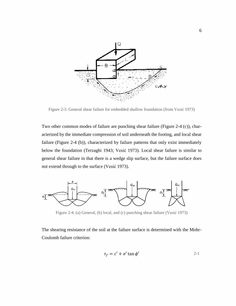
Figure 2-3. General shear failure for embedded shallow foundation (from Vesić 1973)
Two other common modes of failure are punching shear failure (Figure 2-4 (c)), char-
acterized by the immediate compression of soil underneath the footing, and local shear
failure (Figure 2-4 (b)), characterized by failure patterns that only exist immediately
below the foundation (Terzaghi 1943; Vesić 1973). Local shear failure is similar to
general shear failure in that there is a wedge slip surface, but the failure surface does
not extend through to the surface (Vesić 1973).
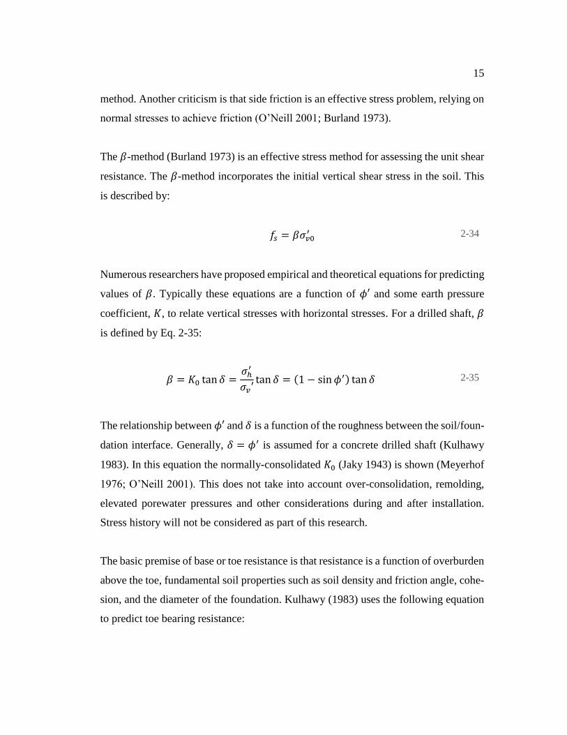
Figure 2-4. (a) General, (b) local, and (c) punching shear failure (Vesić 1973)
The shearing resistance of the soil at the failure surface is determined with the Mohr-
Coulomb failure criterion:
𝜏𝑓 = 𝑐′ + 𝜎′ tan 𝜙′ 2-1

7
where 𝜏𝑓 is the shear stress at failure, c’ is the cohesion in the soil, 𝜎′ is the effective
stress and 𝜙′ is the friction angle. With the Mohr-Coloumb failure criterion, Terzaghi
(1943) proposed a bearing capacity for plane-strain failure of a strip (continuous) foot-
ing, and modified equations for square and circular footings. The ultimate bearing ca-
pacity equation is described in the equations below:
𝑞𝑢𝑙𝑡 = 𝑐′𝑁𝑐 + 𝜎𝑧𝐷′ 𝑁𝑞 + 0.5𝛾′𝐵𝑁𝛾 for continuous footings 2-2
𝑞𝑢𝑙𝑡 = 1.3𝑐′𝑁𝑐 + 𝜎𝑧𝐷′ 𝑁𝑞 + 0.4𝛾′𝐵𝑁𝛾 for square footings 2-3
𝑞𝑢𝑙𝑡 = 1.3𝑐′𝑁𝑐 + 𝜎𝑧𝐷′ 𝑁𝑞 + 0.3𝛾′𝐵𝑁𝛾 for circular footings 2-4
where 𝑐′ is the cohesion of a soil, 𝜎𝑧𝐷′ is the vertical effective stress at the depth of
footing embedment, 𝛾′ is the effective unit weight, 𝐵 is the footing width, and
𝑁𝑐, 𝑁𝑞 , and 𝑁𝛾 are bearing capacity factors. Theses equations were derived from limit
equilibrium, satisfying force and moment equilibrium. The active zone is loaded, push-
ing the logspiral and passive zone, which resist movement by passive and shear forces.
The bearing capacity factors from his derivation are in Eqs. 2-5, 2-7, and 2-8. Equations
for 𝑁𝑐 and 𝑁𝑞 had already been established by Prandtl (1920) and Reissner (1924) in
Eqs. 2-5 and 2-6, respectively. Note that as 𝜙′ → 0° 𝑁𝑐 = 5.14 for Terzaghi (1943)
and = 5.7 for Prandtl (1920).
Prandtl (1920)
𝑁𝑐 = (𝑁𝑞 − 1) cot 𝜙′ 2-5
Reissner (1924)
𝑁𝑞 = 𝑒𝜋 tan 𝜙′tan2(45° + 𝜙′/2) 2-6
Terzaghi (1943)
𝑁𝑞 =
𝑒(270°−𝜙′) tan 𝜙′
2 cos2 (45° +𝜙′2 )
2-7

8
𝑁𝛾 =
1
2tan 𝜙′ (
𝐾𝑃𝛾
cos2 𝜙′− 1) 2-8
where 𝐾𝑝𝛾 is the passive earth pressure coefficients and all other variables are as pre-
viously defined.
2.1.2. Various Improvements on Bearing Capacity Equation
Many researchers have modified the expressions within the general bearing capacity
equation proposed by Terzaghi in 1943. Some works have modified the bearing capac-
ity factors, 𝑁𝛾, 𝑁𝑐, and, 𝑁𝑞, while others have added additional terms, modifying the
equation for shape, inclination, and depth factors (Meyerhof 1961; Hansen 1970; De
Beer 1970; Vesić 1973; Kumbhojkar 1993). This section will only cover a few modi-
fications that have been proposed. Factors concerning inclination and slope inclination
will not be included in this literature review.
In 1961, Meyerhof introduced a revised 𝑁𝛾. The equation for this factor is:
𝑁𝛾 = (𝑁𝑞 − 1) tan(1.4𝜙) 2-9
His later work (1963) also included shape factors and depth factors, accounting for the
different shapes of rectangular footings and embedment depths.
Meyerhof Shape Factors:
𝑠𝑐 = 1 + 0.2𝑁𝜙𝐵/𝐿 2-10
𝑠𝑞 = 𝑠𝛾 = 1 if 𝜙 = 0° 2-11
𝑠𝑞 = 𝑠𝛾 = 1 + 0.1𝑁𝜙𝐵/𝐿 if 𝜙 > 10° 2-12
Meyerhof Depth Factors:
𝑑𝑐 = 1 + 0.2√𝑁𝜙𝐷/𝐵 2-13

9
𝑑𝑞 = 𝑑𝛾 = 1 if 𝜙 = 0° 2-14
𝑑𝑞 = 𝑑𝛾 = 1 + 0.1√𝑁𝜙𝐷/𝐵 if 𝜙 > 10° 2-15
where 𝑁𝜙 = tan2 (1
4𝜋 +
1
2𝜙), which is the friction angle bearing capacity factor. As
mentioned, the framework Terzaghi (1943) proposed neglecting shearing resistance
from soil above the depth of embedment (shown in Figure 2-3). The depth factors from
Eqs. 2-13, 2-14, and 2-15 allow for the consideration of additional shear strength from
the previously neglected soil. For these shape and depth factors, linear interpolation
must be used if the friction angle is between 0 and 10 degrees.
Eqs. 2-10 – 2-15 are intended to modify Terzaghi’s equation for continuous (strip)
footings, Eq. 2-2. Considering these additional factors, the predicted ultimate bearing
capacity for a rectangular shallow foundation becomes:
𝑞𝑢𝑙𝑡 = 𝑐′𝑁𝑐𝑠𝑐𝑑𝑐 + 𝜎𝑧𝐷′ 𝑁𝑞𝑠𝑞𝑑𝑞 + 0.5𝛾′𝐵𝑁𝛾𝑠𝛾𝑑𝛾 2-16
In 1970, Hansen proposed different factors to be used in Eq. 2-16. His work includes
modified shape and depth factors, and another expression for 𝑁𝛾 based entirely on em-
pirical data from previous researchers.
Hansen Shape Factors:
𝑠𝑐 = 1 + 0.2𝐵/𝐿 2-17
𝑠𝑞 = 1 + sin(𝜙) 𝐵/𝐿 2-18
𝑠𝛾 = 1 − 0.4𝐵/𝐿 2-19
Hansen Depth Factors:
𝑑𝑐 = 1 + 0.4𝑘 2-20
𝑑𝛾 = 1 2-21
𝑑𝑞 = 1 + 2 tan 𝜙(1 − sin 𝜙)2𝑘 2-22

10
𝑘 = [
𝐷
𝐵 if
𝐷
𝐵≤ 1
tan−1 (𝐷
𝐵) if
𝐷
𝐵> 1
2-23
Hansen 𝑵𝜸
𝑁𝛾 = 1.5(𝑁𝑞 − 1) tan 𝜙 2-24
Vesić (1973) also established new bearing capacity factors to be used in Terzaghi’s
bearing capacity equation. His considerations were made on the basis of experimental
load tests:
Vesić Shape Factors:
𝑠𝑐 = 1 + (𝐵/𝐿)(𝑁𝑞/𝑁𝑐) 2-25
𝑠𝑞 = 1 + tan(𝜙) 𝐵/𝐿 2-26
𝑠𝛾 = 1 − 0.4𝐵/𝐿 2-27
Vesić 𝑵𝜸
𝑁𝛾 = 2(𝑁𝑞 + 1) tan 𝜙 2-28
Figure 2-5. Comparison of different Nγ factors. (Left: lin-lin ordinate, Right: lin-log ordinate)
0 10 20 30 40
50
100
150
200
Meyerhof (1961)
Vesic (1973)
Hansen (1970)
Kumbhojkar (1993)
Friction Angle [deg]
Be
arin
g C
apac
ity F
acto
r
0 10 20 30 400.1
1
10
100
1 103
Meyerhof (1961)
Vesic (1973)
Hansen (1970)
Kumbhojkar (1993)
Friction Angle [deg]

11
Figure 2-1 compares the above three mentioned 𝑁𝛾 factors and the 𝑁𝛾 from Kumbho-
jkar (1993). Each method shows agreement for small friction angles (on a linear scale),
but the methods diverge for larger friction angles. Plotting on a logarithmic scale indi-
cates that the magnitude of difference between values at small friction angles is greater
than for large friction angles.
Meyerhof (1955) was the first to propose a solution for effective unit weight when the
groundwater table exists close to the base of the foundation. He proposed that soil unit
weight vary linearly between 𝛾𝑏 and 𝛾𝑚 for groundwater table depths of D (depth of
embedment) and D + B (footing width) respectively. This is summarized by Equation
2-29. Here 𝛾𝑏 is the buoyant unit weight of the soil and 𝛾𝑚 is the material unit weight
of the soil. This assumption is often still made in practice (Salgado 2008).
𝛾′ = [
𝛾𝑏 = 𝛾𝑠𝑎𝑡 − 𝛾𝑤 if 𝑧𝑤 < 𝐷
𝛾𝑏 +𝑧𝑤−𝐷
𝐵(𝛾𝑚 − 𝛾𝑏) if 𝐷 ≤ 𝑧𝑤 ≤ 𝐷 + 𝐵
𝛾𝑚 if 𝑧𝑤 > 𝐷 + 𝐵
2-29
2.1.3. Recent Developments
Recently, researchers have begun studying the effects of partial saturation and suction
stress in foundation performance through foundation load tests in partially saturated
soils (Steensen-Bach et al. 1987; Oloo 1997; Costa et al. 2003; Mohamed and Vanapalli
2006; Vanapalli and Mohamed 2013; Wuttke et al. 2013) and by continued modifica-
tion of the conventional bearing capacity equation (Vanapalli and Mohamed 2007; Oh
and Vanapalli 2008; Vahedifard and Robinson 2015) discussed in the previous section.
These researchers have shown that partially saturated soils, especially silts and clays,
often have bearing capacities greater than the predicted bearing capacity for a com-
pletely dry or completely saturated soil.

12
To account for partial saturation, the cohesion term is typically modified within the
bearing capacity equation to account for apparent cohesion caused by suction stresses
(Fredlund et al. 2012; Vanapalli and Mohamed 2007; Vahedifard and Robinson 2015).
Thus, unsaturated soil mechanics can be easily integrated into the convention bearing
capacity framework. With this consideration, Fredlund et al. (2012) suggest a stress
state variable approach, which uses a constant, 𝜙𝑏, (Fredlund 1978), which is a friction
angle that describes the contribution of strength due to partial saturation for the soil.
This contribution to strength is discussed more closely in Section 2.3.5.
Vanapalli and Mohamed (2007) derived a closed-form solution based on the Fredlund
(1978) 𝜙𝑏 expression. The final closed-form solution for the ultimate bearing capacity
of a shallow foundation in unsaturated soils is:
𝑞𝑢𝑙𝑡 = [𝑐′ + (𝑢𝑎 − 𝑢𝑤)𝑏(1 − 𝑆𝜓) tan 𝜙′ + (𝑢𝑎 −
𝑢𝑤)𝐴𝑉𝑅𝑆𝜓 tan 𝜙′] 𝑁𝑐 [1 + (𝑁𝑞
𝑁𝑐) (
𝐵
𝐿)] + 0.5𝐵𝛾𝑁𝛾 [1 − 0.4
𝐵
𝐿]
2-30
In this work, 𝑢𝑎 and 𝑢𝑤 are the air and water pressures within soil pores (the difference
is known as matric suction), (𝑢𝑎 − 𝑢𝑤)𝑏 is the air entry value (or the pressure differ-
ence at which air enters the soil pores at a significant rate), (𝑢𝑎 − 𝑢𝑤)𝐴𝑉𝑅 is the average
matric suction at the bottom of the foundation and stress bulb, 𝑆 is the average degree
of saturation, and finally 𝜓 is a bearing capacity fitting parameter. There are two things
to note about Equation 2-30: (1) two additional terms have been added to the cohesion
term c', (𝑢𝑎 − 𝑢𝑤)𝑏(1 − 𝑆𝜓) tan 𝜙′ captures the contribution of strength due to matric
suctions less than the air-entry value, while (𝑢𝑎 − 𝑢𝑤)𝐴𝑉𝑅𝑆𝜓 tan 𝜙′ captures the con-
tribution of strength due from matric suctions that are greater than the air-entry value;
and (2) additional strength due to matric suction is nonlinear, thus, tan 𝜙𝑏 is replaced
by 𝑆𝜓 and tan 𝜙′. In general, this equation agrees well with the laboratory results pre-
sented in the original paper.

13
Vanapalli and Mohamed (2013) and Vahedifard and Robinson (2015) have modified
Equation 2-30 to account for embedment depth and hydrostatic (steady) flow, which
manifests in the (𝑢𝑎 − 𝑢𝑤) expressions. This modified equation is:
𝑞𝑢𝑙𝑡 = {𝑐′ + (𝑢𝑎 − 𝑢𝑤)𝑏(1 − 𝑆𝑒,𝐴𝑉𝑅) tan 𝜙′ + [(𝑢𝑎 − 𝑢𝑤)𝑆𝑒]𝐴𝑉𝑅 tan 𝜙′}𝑁𝑐𝜉𝑐
+ 𝑞0𝑁𝑞𝜉𝑞 + 0.5𝛾𝐵𝑁𝛾𝜉𝛾 2-31
𝑆𝜓 has been replaced with 𝑆𝑒, the effective saturation, which is 𝑆𝑒 = (𝑆 − 𝑆𝑟)/(1 − 𝑆𝑟).
𝑆𝑟 is the residual saturation of the soil, which is the minimum amount of water the soil
pores will retain. Here, matric suction 𝑢𝑎 − 𝑢𝑤 and effective saturation 𝑆𝑒 are averaged
across a foundation stress bulb, which is considered to be from a depth D to D + 1.5B.
2.2. Deep Foundations
2.2.1. Analytical Theory
The strength and settlement of a deep foundation is a function of multiple factors, rang-
ing from the method of installation to the properties of the soil (Meyerhof 1976). The
ultimate bearing load is difficult to determine because it can only be achieved when the
foundation is in a plunging failure (Salgado 2008). While ultimate bearing load is used
in the literature, it is difficult to attain in practice as it requires very large loads and may
also not be possible due to soil hardening at the toe. Often, deep foundations capacities
are determined against serviceability requirements (limitations on total or differential
settlement or deflection). Ultimate resistance of a pile may be expressed in terms of the
toe bearing resistance, Qt, and the side resistance (skin friction or shaft), Qs. The ulti-
mate resistance of a pile is:
𝑄𝑢 = 𝑄𝑡 + 𝑄𝑠 = 𝑞𝑡𝐴𝑡 + ∑ 𝑓𝑠𝐴𝑠 2-32
where 𝑞𝑡 is the average unit bearing resistance across the area 𝐴𝑡 and 𝑓𝑠 is the unit side
resistance for a layer of soil with a surface area 𝐴𝑠 (Meyerhof 1976). Conceptually, this

14
equation implies that the deep foundation distributes the applied load 𝑄 first through
friction on the side of the foundation, with continual dissipation of load with depth
(O’Neill 1987). Eventually, the remaining force within the pile is applied at the toe.
Before toe bearing resistance can be fully mobilized, the limit of shaft resistance must
be achieved.
Side shear resistance requires horizontal stresses (or the stresses normal to the pile sur-
face) to develop friction (Burland 1973). While effective vertical stresses are relatively
easy to estimate and calculate, effective horizontal stresses are significantly more dif-
ficult, requiring the assumption of earth pressure coefficients. The earth pressure coef-
ficient 𝐾 is not simply just a function of soil type, but also time after installation, depth,
stress history, porewater conditions any many other conditions (O’Neill 2001). It is
difficult to characterize the effective stresses in partially saturated soils due to suction
stresses. Suction stresses may exist in partially saturated soil (clays and silts) causing
tension cracking to occur and lateral earth pressure coefficients to decrease (Lu and
Likos 2004). Once an estimation of 𝐾 is made, the maximum unit side resistance 𝑓𝑚𝑎𝑥
can be determined.
There are two popular method for calculating shaft friction of drilled shafts and piles,
the 𝛼 and 𝛽 method (Skempton 1959; Burland 1973). The 𝛼 method (Skempton 1959)
is a total stress solution used to evaluate the undrained shear strength in saturated clays.
This method is described by:
𝑓𝑠 = 𝛼𝑠𝑢 2-33
Although this is a popular method for calculating shaft resistance, there is little funda-
mental justification in its favor. Values for 𝛼 should not be extrapolated between pile
types and varying ground conditions (Burland 1973). The 𝛼 method has been criticized
because undrained shear strength is not a unique property, but is a function of loading
15
method. Another criticism is that side friction is an effective stress problem, relying on
normal stresses to achieve friction (O’Neill 2001; Burland 1973).
The 𝛽-method (Burland 1973) is an effective stress method for assessing the unit shear
resistance. The 𝛽-method incorporates the initial vertical shear stress in the soil. This
is described by:
𝑓𝑠 = 𝛽𝜎𝑣0′ 2-34
Numerous researchers have proposed empirical and theoretical equations for predicting
values of 𝛽. Typically these equations are a function of 𝜙′ and some earth pressure
coefficient, 𝐾, to relate vertical stresses with horizontal stresses. For a drilled shaft, 𝛽
is defined by Eq. 2-35:
𝛽 = 𝐾0 tan 𝛿 =𝜎ℎ
′
𝜎𝑣′tan 𝛿 = (1 − sin 𝜙′) tan 𝛿 2-35
The relationship between 𝜙′ and 𝛿 is a function of the roughness between the soil/foun-
dation interface. Generally, 𝛿 = 𝜙′ is assumed for a concrete drilled shaft (Kulhawy
1983). In this equation the normally-consolidated 𝐾0 (Jaky 1943) is shown (Meyerhof
1976; O’Neill 2001). This does not take into account over-consolidation, remolding,
elevated porewater pressures and other considerations during and after installation.
Stress history will not be considered as part of this research.
The basic premise of base or toe resistance is that resistance is a function of overburden
above the toe, fundamental soil properties such as soil density and friction angle, cohe-
sion, and the diameter of the foundation. Kulhawy (1983) uses the following equation
to predict toe bearing resistance:

16
𝑞𝑢𝑙𝑡 = 𝑐′𝑁𝑐𝜁𝑐𝑠𝜁𝑐𝑟𝜁𝑐𝑑 +
1
2𝐵𝛾𝑁𝛾𝜁𝛾𝑠 𝜁𝛾𝑟𝜁𝛾𝑑 + 𝑞𝑁𝑞𝜁𝑞𝑠𝜁𝑞𝑟𝜁𝑞𝑑 2-36
where 𝑐′ is cohesion, 𝛾 is the average soil unit weight, and 𝑞 is the effective vertical
stress at the toe. The bearing capacity factors for Eq. 2-36 are:
𝑁𝑞 = 𝑒𝜋 tan 𝜙 tan2(45° + 𝜙/2) 2-37
𝑁𝑐 = (𝑁𝑞 − 1) cot 𝜙 2-38
𝑁𝛾 = 2(𝑁𝑞 + 1) tan 𝜙 2-39
As with shallow foundation bearing capacity theory, as 𝜙 → 0°, 𝑁𝑐 → 5.14. For un-
drained loading in most clays, the bearing capacity equation reduces to approximately
𝑞𝑢𝑙𝑡 = 9𝑠𝑢. Correction factors used in Eq. 2-36 were originally proposed by Vesić
(1975) and Hansen (1970). The shape, depth, and rigidity factors are as follows:
Shape Factors:
𝜁𝑐𝑠 = 1 + 𝑁𝑞/𝑁𝑐 2-40
𝜁𝛾𝑠 = 0.6 2-41
𝜁𝑞𝑠 = 1 + tan 𝜙 2-42
Depth Factors:
𝜁𝑐𝑑 = 𝜁𝑞𝑑 − [
1 − 𝜁𝑞𝑑
𝑁𝑐 tan 𝜙] 2-43
𝜁𝛾𝑑 = 1 2-44
𝜁𝑞𝑑 = 1 + 2 tan 𝜙 (1 − sin 𝜙)2 [(𝜋
180) tan−1(𝐷/𝐵)] 2-45
Rigidity Factors:
𝜁𝑐𝑟 = 𝜁𝑞𝑟 − [
1 − 𝜁𝑞𝑟
𝑁𝑐 tan 𝜙] ≤ 1 2-46
𝜁𝛾𝑟 = 𝜁𝑞𝑟 2-47

17
𝜁𝑞𝑟 = exp{[−3.8 tan 𝜙]
+ [(3.07 sin 𝜙)(log10 2 𝐼𝑟𝑟)/(1 + sin 𝜙) ]} ≤ 1 2-48
The rigidity factors, originally proposed by Vesić (1975), require a solution for Irr, the
reduced rigidity index, Ir, the rigidity index, and Irc, the critical rigidity index:
𝐼𝑟𝑟 =
𝐼𝑟
1 + 𝐼𝑟Δ 2-49
𝐼𝑟 =
𝐸
2(1 + 𝜈𝑑)𝑞𝑎 tan 𝜙 2-50
𝐼𝑟𝑐 = 0.5 exp[2.85 cot(45° − 𝜙/2)] 2-51
In these equations, 𝑞𝑎 is the average stress between 𝐷 and 𝐷 + 𝐵, 𝐸 is the approximate
modulus of elasticity for the soil, 𝜈 is Poisson’s ratio, and Δ is the volumetric strain. Δ
and 𝜈𝑑 have been estimated by Trautmann and Kulhawy (1987) as:
Δ ≅ 0.005(1 − 𝜙𝑟𝑒𝑙) (𝑞𝑎
𝑝𝑎) 2-52
𝜈𝑑 = 0.1 + 0.3𝜙𝑟𝑒𝑙 2-53
𝜙𝑟𝑒𝑙 =
𝜙′ − 25°
45° − 25° 2-54
𝜙𝑟𝑒𝑙 is limited to the values of 0 and 1. Δ is limited to 10. One last check is required
for this method and that is to compare 𝐼𝑟𝑟 to the critical rigidity index, 𝐼𝑟𝑐. If 𝐼𝑟𝑟 > 𝐼𝑟𝑐
then 𝜁𝑐𝑟 = 𝜁𝛾𝑟 = 𝜁𝑞𝑟 = 1. Otherwise, 𝜁𝑐𝑟 = 𝜁𝛾𝑟 = 𝜁𝑞𝑟 < 1 as calculated, reducing the
toe resistance.

18
2.2.2. Recent Developments
Conventional foundation design typically considers the case where soil is completely
saturated beneath the groundwater table and either partially saturated (or wet), for fine-
grained soils, or dry, for coarse-grained soils, above the groundwater table (Vanapalli
and Taylan 2012). Suction stress is neglected in the calculation of effective stress. This
approach is conservative, as it does not consider the effects of partial saturation and
suction stress.
Vanapalli and Taylan (2011) proposed modifications to the 𝛼 and 𝛽 method such that
the effects of partial saturation and suction stresses were included. For a shaft embed-
ded in fine-grained soils, they proposed that:
𝑓𝑠 = 𝛼𝑠𝑢,𝑠𝑎𝑡 [1 +(𝑢𝑎 − 𝑢𝑤)
(𝑃𝑎
101.3 kPa)
𝑆𝜈
𝜇 ] 2-55
(𝑢𝑎 − 𝑢𝑤) is the matric suction, 𝑆 is the degree of saturation, 𝜈 and 𝜇 are fitting pa-
rameters, and 𝑃𝑎 is atmospheric pressure. The above equation implies that if either ma-
tric suction is zero (which occurs near the groundwater table) or saturation is zero
(which occurs at some distance above the groundwater table), there is no additional
frictional resistance in the unsaturated zone.
Vanapalli and Taylan (2011) proposed a modification to the 𝛽-method, capturing the
effects of unsaturated soil mechanics. The researchers suggested that the shaft re-
sistance be captured into two components: (1) frictional resistance due to horizontal
effective stress; and (2) apparent cohesion due to suction. That equation is:
𝑓𝑠 = 𝛽𝜎𝑧′ + (𝑢𝑎 − 𝑢𝑤)(𝑆𝜅)(tan 𝛿′) 2-56

19
where 𝜅 is a fitting parameter used for shear strength and the other terms are as previ-
ously described. In this equation, additional frictional resistance from suction stresses
are considered separately from the effective stress term. To avoid considering suction
stress twice it is important to note that the effective stress term does not include suction
stress.
2.3. Mechanics of Unsaturated Soils
2.3.1. Soil Water Characteristic Curve
Many phenomena present in soil can be explained through the lenses of unsaturated
soil mechanics. Unsaturated soil mechanics integrates the presence of an air phase, wa-
ter phase, and solid phase into one coherent framework. This section will begin with a
discussion on equations that describe the amount of water in soil pores, which also
indicates the amount of air in the pores.
Soil water characteristic curves (also known as soil water retention curves) describe the
relationship between soil suction and water content (Lu and Likos 2004). Several mod-
els have been proposed to fit discrete laboratory data and to continuously describe the
soil water characteristic curve. (Brooks and Corey 1964; van Genuchten 1980; Fred-
lund and Xing 1994). van Genuchten (1980) proposed Eq. 2-57 as a model for the soil
water characteristic curve (SWCC). His work allows for the prediction of effective sat-
uration and normalized water content as a function of matric suction. The equation is
as follows:
Θ = 𝑆𝑒 = [
1
1 + (𝛼𝜓)𝑛]
𝑚
2-57
In this equation, 𝛼, m and n are fitting parameters, however 𝛼 is often considered to be
(or related to) the inverse of the air entry value, or the pressure at which the air-phase
begins to fill the pores at a greater rate. To simplify the expression (which is useful

20
when fitting curves to data) van Genuchten defined 𝑚 = 1 −1
𝑛 to satisfy the Mualem
(1976) hydraulic conductivity model or 𝑚 = 1 −2
𝑛 to satisfy the Burdine (1953) hy-
draulic conductivity model. The units of 𝛼 are kPa-1, or m-1 when considering pressure
heads. Matric suction 𝜓 is defined as the difference between the pressure of a gas phase
and liquid phase, or 𝑢𝑎 − 𝑢𝑤. The normalized water content Θ and effective saturation
𝑆𝑒 are defined by Eq. 2-58.
Θ =
𝜃 − 𝜃𝑟
𝜃𝑠 − 𝜃𝑟= 𝑆𝑒 =
𝑆 − 𝑆𝑟
1 − 𝑆𝑟 2-58
where 𝜃 is the volumetric water content, 𝜃𝑠 is the saturated water content, 𝜃𝑟 is the
residual water content, 𝑆 is the soil saturation, and 𝑆𝑟 is the residual saturation. The
saturated water content is the maximum water content that the soil pores can contain
while the residual water content is the minimum water content that the pores retain.
The soil water characteristic curve, as defined by Eq. 2-57, is useful in defining the
quantity of water that exist in soil pores as a function of the matric suction. Further, if
the quantity of water contained in the pores are known, then suction stress (which dif-
fers from matric suction) can be predicted.
2.3.2. Particle Level Principles
Unsaturated soil mechanics is best understood when explained at a granular scale. Fig-
ure 2-6 below shows a soil water characteristic curve, as described in Section 2.3.1,
and a diagram for two particles in contact with water between contacts.
21
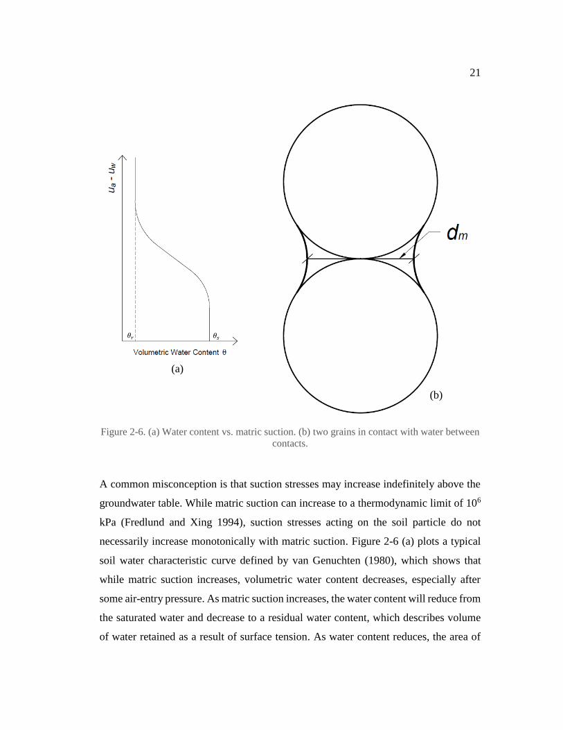
Figure 2-6. (a) Water content vs. matric suction. (b) two grains in contact with water between
contacts.
A common misconception is that suction stresses may increase indefinitely above the
groundwater table. While matric suction can increase to a thermodynamic limit of 106
kPa (Fredlund and Xing 1994), suction stresses acting on the soil particle do not
necessarily increase monotonically with matric suction. Figure 2-6 (a) plots a typical
soil water characteristic curve defined by van Genuchten (1980), which shows that
while matric suction increases, volumetric water content decreases, especially after
some air-entry pressure. As matric suction increases, the water content will reduce from
the saturated water and decrease to a residual water content, which describes volume
of water retained as a result of surface tension. As water content reduces, the area of
𝜃𝑟 𝜃𝑠
(a)
(b)

22
water contact between particles, 𝐴𝑠 =𝜋
4𝑑𝑚
2 , decreases. Consequently, while matric
suctions may be large, the water contact area is small, resulting in limited (or zero)
suction stresses (Lu and Likos 2006; Lu et al. 2009).
Figure 2-7. Forces acting on an individual particle (after Lu and Likos 2004).
Figure 2-7 above summarizes the forces that act on a particle in unsaturated conditions.
Generally, the air pressures acting on a particle are very small. On the contrary, the
water pressure acting on the particle can be very large. As mentioned, matric suction
𝑢𝑎 − 𝑢𝑤 can increase almost indefinitely, however, the suction stresses 𝜎𝑠 cannot. This
is directly related to the water contact area As. This can be summarized as:
𝜎𝑠 = (𝑢𝑎 − 𝑢𝑤)𝑓(𝐴𝑠) = 𝜓 𝑓(𝐴𝑠) = 𝜓𝜒 2-59

23
where 𝑢𝑎 − 𝑢𝑤 and 𝜓 are the matric suction (or the pressure difference between the air
and water phase), and 𝜒 is Bishop’s effective stress parameter – which is a function of
water contact area, and 𝜎𝑠 is the suction stress, or the net interparticle force generated
between of negative pore water pressure and surface tension (Bishop 1959; Lu and
Likos 2004; Lu and Likos 2006). A positive suction will result in a force that tends to
pull particles together, while a negative suction will tend to push particles away (this is
also positive porewater pressure). For fine-grained soil such as clays, suction stress is
also influenced by van der Waal attractions, electric double-layer repulsion, and chem-
ical cementation effects (Lu and Likos 2006). 𝜒 is considered over a range of zero (dry
conditions) to unity (saturated conditions).
Eq. 2-59 introduces the concept of Bishop’s effective stress parameter. This parameter
is intended to capture the variation in suction stress as a function of gradation, soil type,
particle packing – considerations that affect the water contact area, ultimately decreas-
ing suction stress. For sandy soils, the rate at which 𝜒 approaches zero is greater than
the rate at which 𝜓 increases, thus 𝜎𝑠 is generally small for high values of matric suc-
tion. For clayey soils, this is not always the case, causing 𝜎𝑠 to asymptotically approach
a residual value of suction stress (Lu and Likos 2004).
2.3.3. Bishop’s Effective Stress Framework
In 1959, Bishop began the work of characterizing the way partial saturation affects the
state of stress within soil. Conventionally, the effective stress is defined as (Terzaghi
1943):
𝜎′ = 𝜎 − 𝑢𝑤 2-60
where 𝜎′ is the effective stress within the soil, 𝜎 is the net normal stress, and 𝑢𝑤 is the
porewater pressure. This definition works well beneath the groundwater table, where
positive pore water pressures increase linearly with depth. This, however, is not the
case above the ground water table. Soils above the groundwater table are in a state of

24
partial saturation, where nonlinearity arises due to the existence of both a gas and liquid
phase in the pores. To consolidate these two ideas, Bishop introduced an effective stress
parameter 𝜒, which is a function of suction and soil physical properties, capturing non-
linearity in partially saturated soil behavior. Bishop proposed the following equation,
Eq. 2-61.
𝜎′ = 𝜎 − 𝑢𝑎 + 𝜒(𝑢𝑎 − 𝑢𝑤) 2-61
As explained earlier, 𝜒 is unity when saturated and zero when dry. When 𝜒 is equal to
one, the equation is equal to the Terzaghi (1943) definition of effective stress, which is
𝜎′ = 𝜎 − 𝑢𝑎 + 𝑢𝑎 − 𝑢𝑤 = 𝜎 − 𝑢𝑤.
2.3.4. Solutions for Bishop’s Effective Stress Parameter
Since the introduction of this effective stress method, several researchers have sought
to develop solutions/equations for the effective stress parameter 𝜒. Khalili and Khabbaz
(1998) proposed a form based entirely on empirical data. Their results have good cor-
relation to data. The form proposed uses the suction ratio, which is the ratio between
matric suction and the suction at air-entry. Air-entry suction 𝑢𝑒, which is also termed
expulsion pressure, is the suction at which water begins to drain significantly from the
pores, transitioning the soil from a saturated to unsaturated state. The equation for the
Khalili and Khabbaz (1998) effective stress parameter is:
𝜒 = {(
𝑢𝑎 − 𝑢𝑤
𝑢𝑒)
−0.55
for 𝑢𝑎 − 𝑢𝑤 > 𝑢𝑒
1 for 𝑢𝑎 − 𝑢𝑤 ≤ 𝑢𝑒
2-62
This equations implies that before the pore fluid is drained and while the matric suction
is small, the soil behaves as if under conventional soil mechanics principles. Above the
air-entry value, 𝜒 asymptotically approach zero as matric suction increases.
25
Lu and Likos (2004) suggested that 𝜒 is equal to effective saturation, 𝑆𝑒, and the nor-
malized water content, Θ. If this assumption is made, it can be used in conjunction with
the van Genucthen (1980) equation for predicting water content with respect to matric
suction. This theory has been validated experimentally through shear testing on par-
tially saturated soils (Lu and Likos 2006; Lu et al. 2009; Lu et al. 2010). Bishop’s
proposed form was:
𝜒 =
𝑆 − 𝑆𝑟
1 − 𝑆𝑟=
𝜃 − 𝜃𝑟
𝜃𝑠 − 𝜃𝑟 2-63
With the van Genuchten (1980) soil water characteristic curve (SWCC), this equation
becomes:
χ = [
1
1 + (𝛼𝜓)𝑛]
𝑚
2-64
This definition of Bishop’s 𝜒 allows suction stresses, 𝜎𝑠 = 𝜒𝜓, to be related to the soil
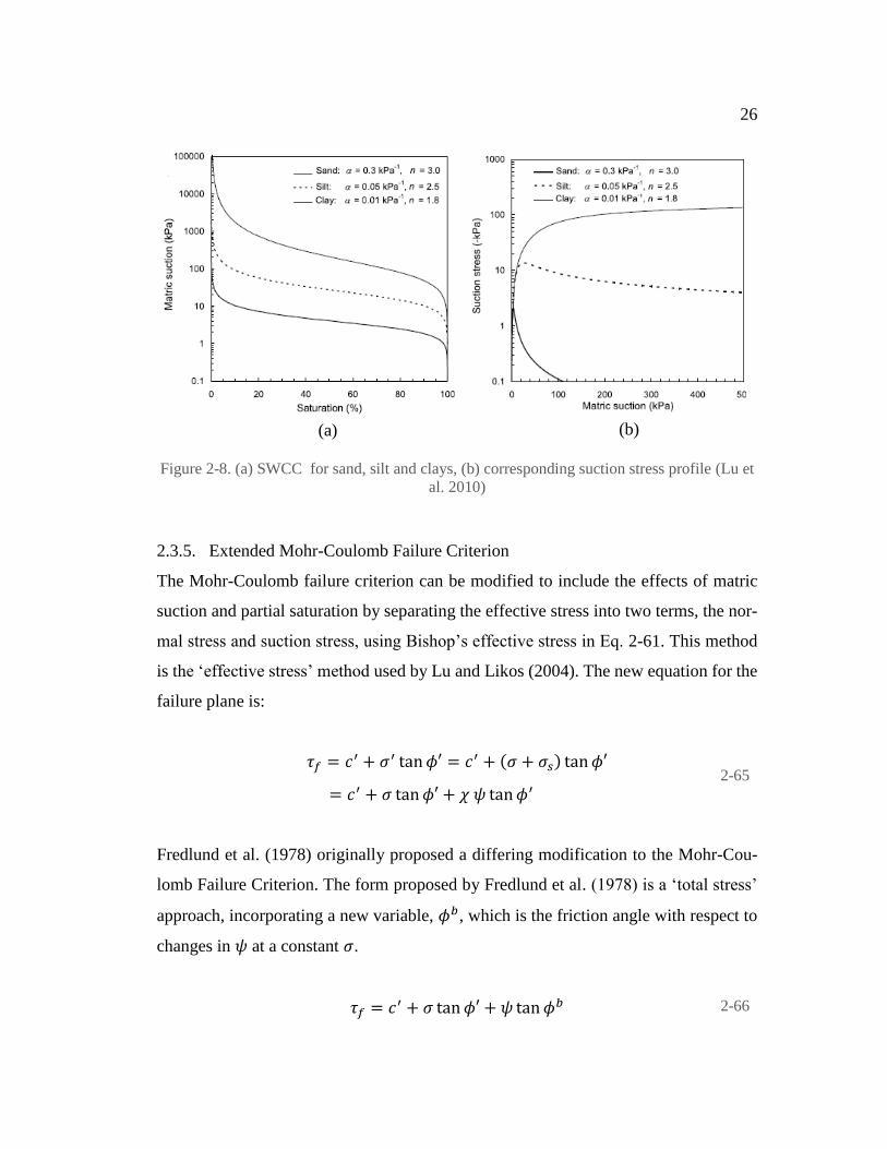
water characteristic curve and corresponding fitting parameters. Figure 2-8 summarizes
the concepts discussed to this point: (a) plot of the soil water characteristic curves ac-
cording to the van Genuchten (1980) model and (b) plot of the suction stress calculated
from Bishop’s 𝜒 defined in Equation 2-64. This figure shows typical behavior for
sands, silts, and clays. Suction stresses in sands typically peak at small matric suction
values and then decrease to zero. Silts may also have a peak suction stress value, but
will either approach an asymptotic value or decrease to zero. Clays will not have a peak
suction stress, but will increase to an asymptotic value of suction (Lu and Likos 2006;
Lu et al. 2010).
26
Figure 2-8. (a) SWCC for sand, silt and clays, (b) corresponding suction stress profile (Lu et
al. 2010)
2.3.5. Extended Mohr-Coulomb Failure Criterion
The Mohr-Coulomb failure criterion can be modified to include the effects of matric
suction and partial saturation by separating the effective stress into two terms, the nor-
mal stress and suction stress, using Bishop’s effective stress in Eq. 2-61. This method
is the ‘effective stress’ method used by Lu and Likos (2004). The new equation for the
failure plane is:
𝜏𝑓 = 𝑐′ + 𝜎′ tan 𝜙′ = 𝑐′ + (𝜎 + 𝜎𝑠) tan 𝜙′
= 𝑐′ + 𝜎 tan 𝜙′ + 𝜒 𝜓 tan 𝜙′ 2-65
Fredlund et al. (1978) originally proposed a differing modification to the Mohr-Cou-
lomb Failure Criterion. The form proposed by Fredlund et al. (1978) is a ‘total stress’
approach, incorporating a new variable, 𝜙𝑏, which is the friction angle with respect to
changes in 𝜓 at a constant 𝜎.
𝜏𝑓 = 𝑐′ + 𝜎 tan 𝜙′ + 𝜓 tan 𝜙𝑏 2-66
(a) (b)

27
Both equations may be recast as:
𝜏𝑓 = 𝑐′ + 𝑐′′ + 𝜎 tan 𝜙′ 2-67
This indicates that the additional strength associated with an increase in suction stresses
can be incorporated into a cohesion parameter, c’’, that is a function of suction. The
Fredlund et al. (1978) form fails to consider the non-linear suction stresses evident in
unsaturated soils. Generally, the form proposed by Lu and Likos (2004; 2006) is more
powerful as it considers non-linearity in the effective stress parameter, 𝜒, while adjust-
ing the effective stress to account for partial saturation. These two approaches, how-
ever, can be consolidated:
𝑐′′ = 𝜓 tan 𝜙𝑏 = 𝜒𝜓 tan 𝜙′ 2-68
where all terms are as previously defined.
2.3.6. Matric Suction Profiles
A matric suction profile must be assumed to implement the effects of unsaturated soils.
Generally, it is assumed that matric suction increases linearly with distance above the
groundwater table. That is, 𝜓 = 𝛾𝑤ℎ, where h is the distance above the groundwater
table. Effects from infiltration and evaporation can also be considered. Using Darcy’s
Law, Lu and Likos (2004) and Lu and Griffiths (2004) provide a derivation for matric
suction as a function of permeability, infiltration/evaporation rates, and height above
the groundwater table which is in Eq. 2-69.
𝜓 = −
1
𝛼[(1 +
𝑞
𝑘𝑠) 𝑒−𝛼𝛾𝑤𝑧 −
𝑞
𝑘𝑠] 2-69
where 𝑞 is the flux rate – evaporation is positive and infiltration negative, 𝑘𝑠 is the
saturated hydraulic conductivity, 𝑧 is the distance above the ground water table, and 𝛼

28
is the inverse of the air-entry pressure (kPa-1), which is related to (or can be assumed
as) the fitting parameter used in the van Genuchten equation.
Eq. 2-69 was derived using the Gardner (1958) one-parameter, exponential model for
hydraulic conductivity:
𝑘 = 𝑘𝑠𝑒−𝛼(𝑢𝑎−𝑢𝑤) 2-70
Figure 2-9. Matric suction profiles at various surface flux boundary conditions for clay (Lu
and Griffiths 2004).
Figure 2-9 shows how a matric suction profile varies with seasonal changes to the flux
conditions. This figure plots water pressure, 𝑢𝑤, which when negative, results in a pos-
itive matric suction 𝜓. It is generally assumed that the matric suction profile with a net
zero flux will behave linearly defined by Eq. 2-71.
𝜓 = 𝛾𝑤𝑧 2-71
where 𝛾𝑤 is the unit weight of water, and 𝑧 is distance above the groundwater table. In
Figure 2-9, when a soil profile is subjected to a positive flux, or evaporation, the matric
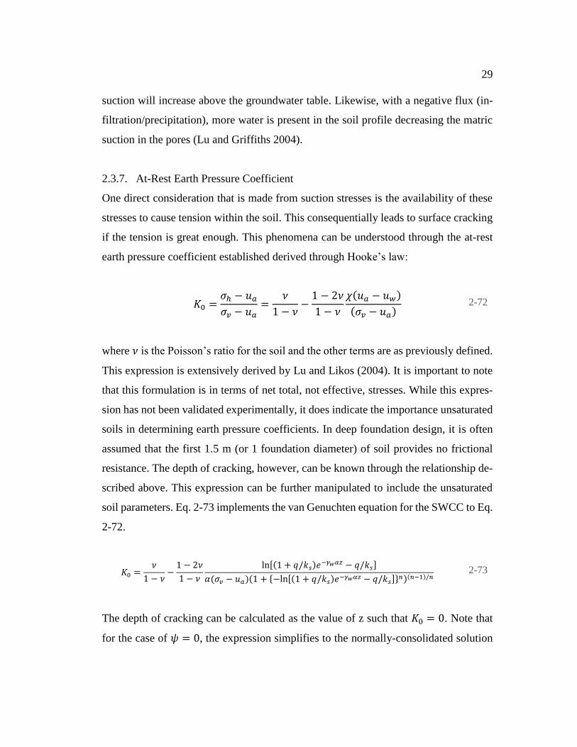
29
suction will increase above the groundwater table. Likewise, with a negative flux (in-
filtration/precipitation), more water is present in the soil profile decreasing the matric
suction in the pores (Lu and Griffiths 2004).
2.3.7. At-Rest Earth Pressure Coefficient
One direct consideration that is made from suction stresses is the availability of these
stresses to cause tension within the soil. This consequentially leads to surface cracking
if the tension is great enough. This phenomena can be understood through the at-rest
earth pressure coefficient established derived through Hooke’s law:
𝐾0 =
𝜎ℎ − 𝑢𝑎
𝜎𝑣 − 𝑢𝑎=
𝜈
1 − 𝜈−
1 − 2𝜈
1 − 𝜈
𝜒(𝑢𝑎 − 𝑢𝑤)
(𝜎𝑣 − 𝑢𝑎) 2-72
where 𝜈 is the Poisson’s ratio for the soil and the other terms are as previously defined.
This expression is extensively derived by Lu and Likos (2004). It is important to note
that this formulation is in terms of net total, not effective, stresses. While this expres-
sion has not been validated experimentally, it does indicate the importance unsaturated
soils in determining earth pressure coefficients. In deep foundation design, it is often
assumed that the first 1.5 m (or 1 foundation diameter) of soil provides no frictional
resistance. The depth of cracking, however, can be known through the relationship de-
scribed above. This expression can be further manipulated to include the unsaturated
soil parameters. Eq. 2-73 implements the van Genuchten equation for the SWCC to Eq.
2-72.
𝐾0 =𝜈
1 − 𝜈−
1 − 2𝜈
1 − 𝜈
ln[(1 + 𝑞/𝑘𝑠)𝑒−𝛾𝑤𝛼𝑧 − 𝑞/𝑘𝑠]
𝛼(𝜎𝑣 − 𝑢𝑎)(1 + {−ln[(1 + 𝑞/𝑘𝑠)𝑒−𝛾𝑤𝛼𝑧 − 𝑞/𝑘𝑠]}𝑛)(𝑛−1)/𝑛 2-73
The depth of cracking can be calculated as the value of z such that 𝐾0 = 0. Note that
for the case of 𝜓 = 0, the expression simplifies to the normally-consolidated solution

30
for 𝐾0 = 𝜈/(1 − 𝜈). If 𝜈𝑢 = 0.5 is used, the expression simplifies to 𝐾0 = 1, which is
expected in undrained, elastic loading conditions.
2.3.8. Discussion of Unsaturated Soil Properties
The van Genuchten (1980) equation describes the soil water characteristic curve, or a
soil’s water retention with respect to matric suction, as a function of five variables. The
first is 𝛼, which has the units of either m-1 or kPa-1. 𝛼 is related inversely to the air entry
pressure or head of a given soil. The second and third variables are 𝜃𝑠 and 𝜃𝑟, which
are the saturated and residual water contents. 𝜃𝑠 is limited to the porosity of a soil. The
last two variables are n and m, which are fitting parameters used to fit Eq. 2-57 to
laboratory data. Another important variable is the saturated hydraulic conductivity ks,
which has units of m/s.
Carsel and Parrish (1988) performed an extensive study on the variation of these un-
saturated soil parameters between the 12 different soil types identified in the USDA
Soil Classification System. This classification system simply describes soil as a func-
tion of percent clay, silts, and sands. Carsel and Parrish (1988) performed many statis-
tical analysis on over 15,000 soils including simple calculations of the mean and stand-
ard deviation of a soil type, and a thorough framework for performing Monte Carlo
simulations. Note, that the Mualem (1976) solution for m = 1 – 1/n was used by these
authors. Table 2-1 presents the average mean and standard deviations for unsaturated
soil parameters by soil texture according to Carsel and Parrish (1988).

31
Table 2-1. Typical unsaturated soil properties by USDA textural class (Carsel and Parrish
1988)
𝜽𝒔 𝜽𝒓 𝜶 (𝐜𝐦−𝟏) 𝑲𝒔 (𝐜𝐦/𝐡𝐫) 𝒏
�̅� 𝑠 �̅� 𝑠 �̅� 𝑠 �̅� 𝑠 �̅� 𝑠
Clay 0.38 0.09 0.068 0.034 0.008 0.012 0.20 0.42 1.09 0.09
Clay Loam 0.41 0.09 0.095 0.010 0.019 0.015 0.26 0.70 1.31 0.09
Loam 0.43 0.10 0.078 0.013 0.036 0.021 1.04 1.82 1.56 0.11
Loamy
Sand 0.41 0.09 0.057 0.015 0.124 0.043 14.59 11.36 2.28 0.27
Silt 0.46 0.11 0.034 0.010 0.016 0.007 0.25 0.33 1.37 0.05
Silt Loam 0.45 0.08 0.067 0.015 0.020 0.012 0.45 1.23 1.41 0.12
Silty Clay 0.36 0.07 0.070 0.023 0.005 0.005 0.02 0.11 1.09 0.06
Silty Clay
Loam 0.43 0.07 0.089 0.009 0.010 0.006 0.07 0.19 1.23 0.06
Sand 0.43 0.06 0.045 0.010 0.145 0.029 29.70 15.60 2.68 0.29
Sandy
Clay 0.38 0.05 0.100 0.013 0.027 0.017 0.12 0.28 1.23 0.10
Sandy
Clay Loam 0.39 0.07 0.100 0.006 0.059 0.038 1.31 2.74 1.48 0.13
Sandy
Loam 0.41 0.09 0.065 0.017 0.075 0.037 4.42 5.63 1.89 0.17
As mentioned, Carsel and Parrish (1988) developed framework for determining appro-
priate unsaturated parameters to be used in Monte Carlo simulations. It is important to
appropriately characterize these properties for several reasons: (1) most of these prop-
erties do not have a normal distribution, but may have lognormal, log ratio, or hyper-
bolic arcsine distributions (Carsel and Parrish 1988); and (2) many of the properties are
interrelated including n, 𝜃𝑟, 𝛼, and 𝑘𝑠. If any of these four variables change, it is more
than likely that one or more of the other three variables would change as a result. The
exception to this is the saturated water content, which is assumed to vary independently

32
from the other variables. This assumption is valid since typical variations in 𝜃𝑠 are
small (generally less than 25%).The procedures developed by Carsel and Parrish (1988)
produce suitable Monte Carlo realizations that considers relationships between each
property while still matching known distributions.
2.4. Summary
Section 2.1 and 2.2 covered the current practice of calculating bearing capacity for
shallow foundations and drilled shafts. Section 2.3 covered the current state of unsatu-
rated soil mechanics in the literature. For shallow foundations, bearing capacity is typ-
ically calculated through closed form equations that are based on some form of the
Terzaghi (1943) bearing capacity equation. Subsequent research have introduced vari-
ous shape and depth factors. For drilled shafts, the 𝛽-method is frequently used to cal-
culate side friction and total side resistance while toe bearing may be calculated through
bearing capacity equations that have a similar form to the shallow foundation bearing
capacity equations.
More recently, researchers have developed solutions to the shallow foundation bearing
capacity equation with respect to matric suctions that are present in a body of partially
saturated soils (Vanapalli and Mohamed 2007; Oh and Vanapalli 2008; Vahedifard and
Robinson 2015). These solutions are based on the Fredlund et al (1978) total stress
approach, but an effective stress approach (Lu and Likos 2004) may be more appropri-
ate. Another issue with these solutions is that average matric suction values are calcu-
lated across the stress bulb. Instead, average apparent cohesion should be calculated
across the failure surface since soils on this plane are being sheared. These solutions
also require an assumption for the air-entry value as well as bearing capacity fitting
parameters. It would be more appropriate to calculate bearing capacity (or apparent
cohesion) directly from the soil water characteristic curve. Vahedifard and Robinson
(2015) introduced a procedure for calculating bearing capacity for steady state flow.
This approach will be used and assessed in this current work for shallow and deep

33
foundations. Variation in overburden, or the effective stress at the depth of embedment,
and average soil unit weight within the failure surface are not considered in the litera-
ture.
Vanapalli and Taylan (2011) have proposed solutions for side resistance for both the
𝛼-method and 𝛽-method. For the 𝛽-method, Vanapalli and Taylan (2011) did not spe-
cifically vary the 𝛽 term in the expression, but instead introduced a separate term to
account for suction stresses. While this is a good assumption for the state of suction
stresses within a body of soil, the net normal horizontal stresses should also be affected
since suction will decrease the at-rest earth pressure coefficient, as discussed in Section
2.3.7. This means that 𝐾0 will decrease (or become zero when cracking), which implies
that 𝛽 should also be reduced.
The state of unsaturated soil mechanics, discussed in Section 2.3, is rapidly changing,
with many publications written within the last decade. Currently, there are two methods
for calculating shear strength with respect to suction: the total stress approach (Fred-
lund et al. 1978), and the effective stress approach (Lu and Likos 2004). For both these
methods, suction is calculated from the soil water characteristic curve (SWCC). These
methods have been validated through laboratory testing (Fredlund et al. 1978; Lu and
Likos 2006; Lu et al. 2009). Expressions for the earth pressure coefficients and steady-
state flow (or flux) in unsaturated soils have not yet been validated experimentally. The
solution for the steady-state flow (Lu and Griffith 2005) is based on the simple Gardner
(1958) solution to hydraulic conductivity, which has been replaced by more numeri-
cally complex solutions. New steady-state flow equations in unsaturated soils should
be developed for newer permeability models to improve the accuracy of assumed ma-
tric suction profiles.
There is a need in both shallow and deep foundations design for simple solutions that
account for the suction in partially saturated soils. This work will develop a simple

34
framework for modifying the conventional shallow foundation bearing capacity and
deep foundation side resistance to account for matric suction and partial saturation.

35
3. Research Objectives and Methodology
3.1. Objectives
The purpose of this study is to explore the theoretical implications of calculating the
bearing capacity of shallow and deep foundations in the presence of unsaturated soils.
This includes using the considerations listed in the Chapter 2: matric suction, infiltra-
tion/evaporation, effective stress parameters to produce suction stresses, surface ten-
sion/cracking, at-rest earth pressure (EP) coefficients, and the unsaturated failure crite-
rion.
For typical shallow foundation design, resistance is derived from three primary com-
ponents: cohesion, unit weight, and surcharge loads. These three components are di-
rectly influenced by the value of the friction angle through bearing capacity factors.
The shape of the failure surface is understood to be a function of friction angle. The
assumption in this work is that the shape of the failure surface does not change as a
function of varying suction stresses and water contents. It would be difficult to assume
changes in the failure surface according the variation in saturation and suction stresses.
To consolidate both unsaturated soil mechanics and shallow foundation design, it is
assumed that an apparent cohesion term from Eq. 2-68 can be directly implemented
into the bearing capacity equation. This is appropriate since the shallow foundation
framework was described according to the Mohr-Coulomb failure criterion. Apparent
cohesion is simply an extension of MC failure surface in the third dimension, with
matric suction as a third stress state variable. Furthermore, the unit weight can be ap-
proximated by finding the average unit weight within the failure surface. The saturation
profile (calculated from the SWCC) can be used to define the unit weight of water as a
function of distance above the groundwater table. The third term, the effective stress at
the depth of embedment, will be calculated by summing the suction stress 𝜎𝑠 and
weight of soil above the base of the shallow foundation when the groundwater table is
beneath the depth of embedment.

36
Considerations for the side resistance of deep foundations are simple in that deep foun-
dations fail vertically across the length of the deep foundation. Toe bearing resistance
is more difficult to approximate and is often near or below the groundwater table in a
dense soil layer. Contribution to strength from partial saturation will be calculated sep-
arately for shaft resistance and toe bearing.
Partial saturation will be considered in shaft resistance by integrating the suction stress
profile for implementation in the 𝛽-method. Furthermore, variation in vertical stresses
can be calculated from the unit weight profiles, which are a function of the saturation
profile derived from the van Genuchten soil water characteristic curve (Eq. 2-57). The
last consideration in shaft resistance is in the variation of earth pressure coefficients.
Suction stresses present in unsaturated soils will engender a decrease in soil contacts,
especially for near-surface soils. This phenomena will decrease horizontal earth pres-
sures and ultimately produce surface cracking. Eq. 2-73 will be used for K in the 𝛽-
method, allowing a single integrand across the surface of the shaft.
Many equations exist in an effort to predict toe bearing resistance. Toe bearing re-
sistance is usually defined based on settlement requirements since ultimate states are
difficult to achieve. Typically, toe bearing resistance is predicted from either CPT data
(or some similar field test), pile driving data, or bearing capacity equations. For the
consideration of partial saturation in toe bearing (which is only relevant if the toe is
above the groundwater table), bearing capacity equations must be used. In this work
the Vesić toe bearing capacity equations described in Kulhawy et al. (1983) will be
used. The same approach for considering partial saturation in shallow foundations will
be used for the deep foundation bearing capacity equation.
The remainder of this chapter is dedicated to the theoretical development of shallow
foundation bearing capacity and deep foundation side resistance in partially saturated
soils. A modified shallow foundation bearing capacity equation is developed in Section

37
3.2 and a modified 𝛽-method for deep foundation is developed in Section 3.3. Follow-
ing this chapter, the validity of the modified shallow foundation equation is assessed
by comparing measured load tests in Chapter 4. Parametric studies on both the modified
shallow foundation and 𝛽 equations are discussed in Chapter 5. Sensitivity to soil input
parameters, including van Genuchten fitting parameters, for these modified approaches
are discussed in this chapter. Design charts are developed and discussed in Chapter 5.
For consistency throughout this thesis, the Vesić bearing capacity equations will be
used. The modifications proposed to account for partially saturated soil can be applied
to any bearing capacity framework. Further, any definition of 𝜒, the SWCC, and matric
suction profile can be used as well. The Lu et al. (2006) definition of 𝜒, van Genuchten
(1980) SWCC, and Lu and Griffiths (2004) 𝜓-profile are used in this section and in the
remainder of this thesis.
3.2. Shallow Foundations in Unsaturated Soils
3.2.1. Theoretical Development
The general bearing capacity equation for shallow foundations can be modified to ac-
count for partial saturation in three ways: (1) modifying the effective stress at the depth
of embedment (or overburden) term; (2) modifying the soil unit weight term; and (3)
modifying the cohesion term. Overburden can be modified to account for the suction
stresses that exist at the depth of embedment for partially saturated soils. Soil unit
weight in partially saturated soils will vary above the groundwater table due to capil-
larity. An average unit weight can be calculated across the failure surface if the water
content throughout the soil profile is known. Water content is a function of distance
above the groundwater table and can be predicted from the soil water characteristic
curve discussed in Section 2.3.1. Cohesion can be modified to account for apparent
cohesion due to suction stresses across the failure surface. This is a valid assumption
because stresses along the failure surface can be expressed Mohr-Coulomb failure cri-
terion.

38
An assumption made in this work is that the shape of the failure surface is not affected
by suction stresses and variations in soil unit weight due to partial saturation above the
ground water table. Current solutions to the bearing capacity factors are based on the
friction angle and are not a function of variables such as cohesion and unit weight.
Therefore, it is assumed apparent cohesion and suction stresses play no role in varying
the shape of the failure surface. The general bearing capacity equation is in Eq. 3-1.
𝑞𝑢𝑙𝑡 = 𝑐′𝑁𝑐𝑠𝑐𝑑𝑐 + 𝜎𝑧𝐷′ 𝑁𝑞𝑠𝑞𝑑𝑞 + 0.5𝛾′𝐵𝑁𝛾𝑠𝛾𝑑𝛾 3-1
Any of the discussed bearing capacity factors could be selected, but for the sake of
using one framework the Vesić 𝑁𝛾 equation will be used. In the Vesić framework, the
Prandtl (1920) 𝑁𝑐 and Reissner (1924) 𝑁𝑞 equations are used in addition to the Vesić
(1973) 𝑁𝛾 and shape factors, and the Hansen (1970) shape factors. The Vesić depth
factor allows for the consideration of cohesion at the toe of a failure surface in embed-
ded foundations. Cohesion (and apparent cohesion) at the toe is considered in this work.
To account for partial saturation, the general bearing capacity equation is modified in
Eq. 3-2. From here, this equation will be called the modified bearing capacity equation
or the modified approach.
𝑞𝑢𝑙𝑡 = (𝑐′ + 𝑐′′̅̅ ̅)𝑁𝑐𝑠𝑐𝑑𝑐 + 𝑞𝑠𝑁𝑞𝑠𝑞𝑑𝑞 + 0.5𝛾′̅ 𝐵𝑁𝛾𝑠𝛾𝑑𝛾 3-2
where 𝑐′ is the soil cohesion, 𝑐′′̅̅ ̅ is the average apparent cohesion due to suction stresses
across the length of the failure surface, 𝑞𝑠 is the overburden (including the suction
stress), and 𝛾′̅ is the average effective soil unit weight across the area of the failure
surface. The other expressions are as defined in Section 2.1.1. Apparent cohesion, over-
burden, and average effective soil unit weight are defined by Eq. 3-3, 3-4, and 3-5.

39
𝑐′′̅̅ ̅ =
∫ 𝑐′′𝑑𝑙
𝑙
𝑙=
∫ 𝜎𝑠 tan 𝜙′ 𝑑𝑙
𝑙
𝑙=
∫ 𝜓𝜒 tan 𝜙′ 𝑑𝑙
𝑙
𝑙 3-3
𝑞𝑠 = 𝜎𝑧𝐷 + 𝜎𝑠,𝑧𝐷 = 𝜎𝑧𝐷 + (𝜓𝜒)𝑧𝐷 if 𝐷 < 𝑧𝑤
𝑞𝑠 = 𝜎𝑧𝐷 − 𝑢 if 𝐷 ≥ 𝑧𝑤 3-4
𝛾′̅ =
∫ 𝛾′(𝜓)𝑑𝐴
𝐴
𝐴 3-5
where 𝜎𝑠 is suction stress (Section 2.3.2 and 2.3.3), 𝜓 is matric suction (Section 2.3.6),
𝜒 is Bishop’s Chi (Section 2.3.4), 𝑙 is the length of the failure surface, 𝑞𝑠 is the net
normal stress at the depth of embedment, 𝜎𝑠,𝑧𝐷 is the suction stress at the depth of
embedment, 𝐷 is the depth of embedment, 𝑧𝑤 is the depth of the groundwater table, 𝑢
is porewater pressure, 𝐴 is the area contained by the failure surface, and 𝛾′ is the effec-
tive (or buoyant below the groundwater table) unit weight of the soil, which is a func-
tion of matric suction. Apparent cohesion is zero below the groundwater table and pos-
itive above. If the foundation is embedded beneath the groundwater table, pore water
pressure will be used instead of suction stress in Eq. 3-3. Likewise, if the failure surface
extends below the groundwater table, the moist unit weight is used above the ground-
water table and the buoyant unit weight below.
To demonstrate how this approach is implemented, a thorough example of a shallow
foundation failure in partially saturated soil will be considered. The following example
includes soil with the properties listed in Table 3-1.
Table 3-1. Soil properties for theoretical example of shallow foundation bearing capacity in
an unsaturated soil.
Variable 𝑮𝒔 𝜽𝒔 𝜽𝒓 𝜶 𝒏 𝝓′
Value 2.65 0.385 0.0385 0.175 kPa-1 2.5 20°
where 𝐺𝑠 is the specific gravity of the soil, 𝜃𝑠 is the saturated volumetric water content,
𝜃𝑟 is the residual water content, 𝛼 and 𝑛 are van Genuchten fitting parameters and 𝜙′
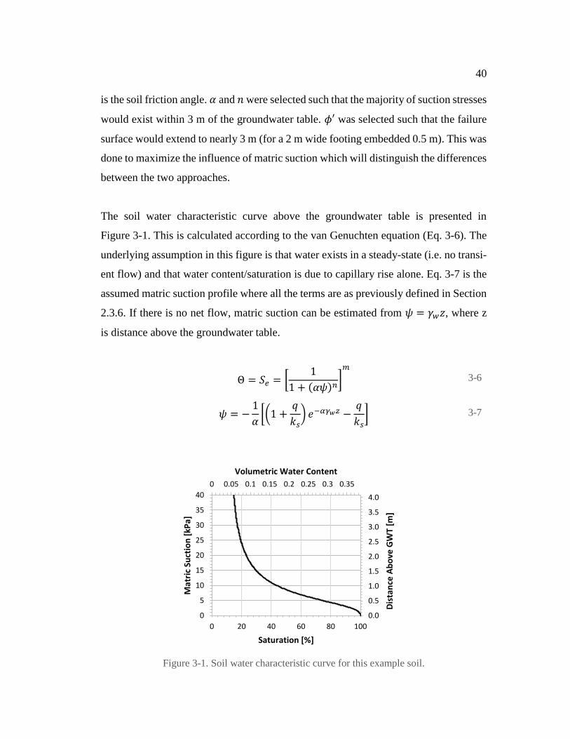
40
is the soil friction angle. 𝛼 and 𝑛 were selected such that the majority of suction stresses
would exist within 3 m of the groundwater table. 𝜙′ was selected such that the failure
surface would extend to nearly 3 m (for a 2 m wide footing embedded 0.5 m). This was
done to maximize the influence of matric suction which will distinguish the differences
between the two approaches.
The soil water characteristic curve above the groundwater table is presented in
Figure 3-1. This is calculated according to the van Genuchten equation (Eq. 3-6). The
underlying assumption in this figure is that water exists in a steady-state (i.e. no transi-
ent flow) and that water content/saturation is due to capillary rise alone. Eq. 3-7 is the
assumed matric suction profile where all the terms are as previously defined in Section
2.3.6. If there is no net flow, matric suction can be estimated from 𝜓 = 𝛾𝑤𝑧, where z
is distance above the groundwater table.
Θ = 𝑆𝑒 = [
1
1 + (𝛼𝜓)𝑛]
𝑚
3-6
𝜓 = −
1
𝛼[(1 +
𝑞
𝑘𝑠) 𝑒−𝛼𝛾𝑤𝑧 −
𝑞
𝑘𝑠] 3-7
Figure 3-1. Soil water characteristic curve for this example soil.
0 0.05 0.1 0.15 0.2 0.25 0.3 0.35
0.0
0.5
1.0
1.5
2.0
2.5
3.0
3.5
4.0
0
5
10
15
20
25
30
35
40
0 20 40 60 80 100
Volumetric Water Content
Dis
tan
ce A
bo
ve G
WT
[m]
Mat
ric
Suct
ion
[kP
a]
Saturation [%]

41
The suction stress profile can also be calculated for the soil in Table 3-1. In the effective
stress approach, suction stress is defined by 𝜎𝑠 = 𝜓𝜒. Using Eq. 3-8 (Lu et al. 2006;
Lu et al. 2009; Lu et al. 2010) to define Bishop’s 𝜒 leads to the suction stress profile in
Figure 3-2.
𝜒 =
𝑆 − 𝑆𝑟
1 − 𝑆𝑟=
𝜃 − 𝜃𝑟
𝜃𝑠 − 𝜃𝑟 3-8
Figure 3-2. Suction stress profile for this example soil.
The groundwater and foundation dimensions are described in Table 3-2. The founda-
tion in this example is a strip footing.
Table 3-2. Foundation and groundwater properties for theoretical example in Chapter 3.
Variable 𝒛𝒘 𝑩 𝑫
Value 3 m 2 m 0.5 m
0.0
0.5
1.0
1.5
2.0
2.5
3.0
3.5
4.0
0
5
10
15
20
25
30
35
40
0 1 2 3 4 5
Dis
tan
ce A
bo
ve G
WT
[m]
Mat
ric
Suct
ion
[kP
a]
Suction Stress [kPa]

42
The Terzaghi failure surface with a friction angle of 20° would extend just above the
groundwater table, as shown in Figure 3-3. In this example, the failure surface extends
to a depth of 2.85 m. The groundwater table was set to a depth of 3 m such that it would
have maximum influence on the foundation performance. This foundation will be
loaded to the ultimate limit state, where continuous plastic flow occurs.
Figure 3-3. Failure surface corresponding to ϕ' = 20°, B = 2 m, and D = 0.5 m.
3.2.2. Considerations for Apparent Cohesion
From Figure 3-2, we can define the saturation of the soil based on the proximity of the
layer to the depth of the groundwater table. Figure 3-4 presents the assumed saturation
profile, colored based on saturation at a depth and superimposed on the failure surface.
This figure shows that while matric suction is assumed to increase linearly above the
groundwater table, saturation, and ultimately suction stress, vary nonlinearly.

43
Figure 3-4. Saturation of the soil profile for the example.
Using this approach, the saturation of the soil can be determined at any point along the
failure surface. This ultimately enables the calculation of average suction stress acting
along the failure surface. Figure 3-5 shows the saturation, as well as its corresponding
apparent cohesion 𝑐′′ = 𝜎𝑠 tan 𝜙′, across the failure surface according to its proximity
from the groundwater table.
Figure 3-5. Failure surface of the shallow foundation, colored by the saturation profile.
100
80
60
40
20
0.91 kPa
1.12 kPa
1.29 kPa
1.38 kPa 1.40 kPa
1.37 kPa 1.27 kPa
1.11 kPa
0.79 kPa

44
From Figure 3-5, suction stress and apparent cohesion can be calculated along the value
surface. Average apparent cohesion can be calculated along the failure surface by mul-
tiplying representative apparent cohesions by the length over which they act, summing
those values, and dividing by the total length (l). This process can be performed for
infinitesimally small increments using Eq. 3-3. Using this equation, 𝑐’’ ̅̅̅̅ is calculated
to be 1.11 kPa. Thus, the entire cohesion term (𝑐′ + 𝑐′′̅̅ ̅) is (0 kPa + 1.11 kPa).
The issue with simply calculating apparent cohesion from the average depth is that 𝜒
behaves extremely nonlinearly (Section 2.3.4), even while 𝜓 behaves linearly above
the groundwater table for 𝑞 = 0 m/s (Section 2.3.6). Other issues are that the ground-
water table may exist within the failure surface, and 𝜒 may be limited due to cavitation
in pores. Consider this: for the previous example, the failure surface extended to a depth
of 2.85 m. Assuming the average failure surface depth is, say, 1.4 m, would the average
apparent cohesion be 0 kPa if the groundwater table was at this depth? No, while there
is no apparent cohesion below the groundwater table, apparent cohesion still exist at
the beginning and end of the failure surface, which will contribute to strength. There-
fore, the apparent cohesion must be averaged across the entire failure surface length,
and cannot be assumed from the average failure surface depth. If the groundwater table
depth was 1.4 m, the average apparent cohesion would be 0.41 kPa.
3.2.3. Considerations for Unit Weight
Similar assumptions can be made for this example in regards to the saturation profile.
Using this profile, the unit weight of water can be estimated throughout the entire fail-
ure surface. The averaged unit weight can be used directly within the bearing capacity
framework.

45
Figure 3-5. Variation in saturation within the failure surface for this example.
The average unit weight can be calculated in a similar way to the average apparent
cohesion. Using the saturation profile in Figure 3-5 (or the SWCC in
Figure 3-1), the moist unit weight profile can be calculated according from Eq. 3-9.
𝛾𝑚 = (𝐺𝑠(1 − 𝜃𝑠) + 𝜃)𝛾𝑤 = (𝐺𝑠(1 − 𝜃𝑠) + 𝜃𝑠𝑆)𝛾𝑤 3-9
where 𝛾𝑚 is the moist unit weight, 𝐺𝑠 is the specific gravity, 𝜃𝑠 is the saturated volu-
metric water content (equal to porosity), 𝜃 is the volumetric water content, 𝑆 is the
saturation, and 𝛾𝑤 is the unit weight of water. Once the unit weight profile is known,
the average unit weight can be calculated by taking a surface integral of unit weight
across the area of the failure surface then dividing by the total area.
𝛾′̅ =
∫ 𝛾′(𝜓)𝑑𝐴
𝐴
𝐴 3-10
𝛾′ is the moist unit weight, defined by Eq. 3-9, above the groundwater table, and the
buoyant unit weight below the groundwater table (which is the saturated unit weight
minus the unit weight of water). From Eq. 3-10, the average unit weight was calculated
80
60
80
40
80
100
80
20
80

46
as 𝛾 = 17.3 kN/m3. It is important to note that the soils above the base of the footing
are not included in this average, but are considered in the overburden term. The Vesić
equation accounts for shearing resistance above the base of the footing, which is con-
sidered in the apparent cohesion expression and implemented through depth factors.
The conventional approach assumes that the average unit weight varies between the
buoyant unit weight when the groundwater table is above the depth of embedment and
a dry/moist unit weight when the groundwater table is greater than the depth of embed-
ment plus the footing width (D + B). For this particular soil, the unit weight using the
conventional approach is estimated to be 16.4 kN/m3, which is a 0.9 kN/m3 difference.
3.2.4. Considerations for Overburden
The third term in Vesić’s bearing capacity equation is overburden. Overburden is the
effective stress at the base of the footing. In the presence of unsaturated soils, this ef-
fective stress will include the effects of suction stress. Overburden is the simplest con-
sideration in the Vesić equation, requiring only knowledge of the soil unit weight above
the footing and the suction stress at the embedment depth. From Figure 3-2, the suction
stress at the depth of embedment is 2.7 kPa. The net normal (total) stress can be calcu-
lated as the integral of the soil unit weight from the surface to the depth of embedment.
This is shown by Eq. 3-11.
𝑞𝑠 = 𝜒𝜓 + ∫ 𝛾(𝑧)𝑑𝑧
𝐷
0
= 𝜎𝑠 + 𝜎𝑡 3-11
The calculated surcharge in this example is 𝑞𝑠 = 11.1 kPa. The conventional approach
would use the estimate 16.4 kN/m3 from the previous section, multiplied by the depth
of embedment (0.5 m), resulting in an 8.2 kPa overburden.
Putting all these considerations together, the modified inputs can be used with the Vesić
equation:

47
𝑞𝑢𝑙𝑡 = (𝑐′ + 𝑐′′̅̅ ̅)𝑁𝑐𝑠𝑐𝑑𝑐 + 𝑞𝑠𝑁𝑞𝑠𝑞𝑑𝑞 + 0.5𝛾′̅ 𝐵𝑁𝛾𝑠𝛾𝑑𝛾
𝑞𝑢𝑙𝑡 = ( 1.12 kPa)𝑁𝑐𝑠𝑐𝑑𝑐 + (11.1 kPa)𝑁𝑞𝑠𝑞𝑑𝑞 + 0.5(17.3 kN/m3)𝐵𝑁𝛾𝑠𝛾𝑑𝛾
The bearing capacity is calculated to be 187 kPa. If the unmodified approach was used,
the bearing capacity would be calculated as 144 kPa. Thus, the modified approach pre-
dicts a 30% increase in bearing capacity relative to the conventional approach.
3.3. Deep Foundations in Unsaturated Soils
3.3.1. Theoretical Development
As discussed in Section 3.1, the effects of partial saturation on side resistance and toe
bearing are different, requiring two separate calculations. For side resistance, suction
stresses will increase strength along the length of the deep foundation since failure oc-
curs across this surface. This failure, described by the 𝛽-method, can simply be reduced
to the extended Mohr-Coulomb failure criterion (Section 2.3.5). Suction stresses, how-
ever, can work detrimentally against the performance of side resistance since the at-
rest earth pressure coefficient will decrease due to suction above the groundwater table
(Section 2.3.7). Considerations for toe bearing in partially saturated soils can be treated
like shallow foundations, requiring an assumption for apparent cohesion, surcharge and
unit weight. Figure 3-6 visualizes the different modes of resistance – side resistance
and toe bearing resistance – used in this work.

48
Figure 3-6. Sketch of the conceptual deep foundation considered in this work.
As mentioned, resistance for deep foundations accumulates along the length of the shaft
and at the toe. The shear resistance at failure in partially saturated soils can be described
by the extended Mohr-Coulomb failure criterion in Eq. 3-12.
𝜏𝑓 = 𝑐′ + 𝜎ℎ′ tan 𝛿 = 𝑐′ + 𝜎ℎ tan 𝛿 + 𝜎𝑠 tan 𝛿 3-12
where 𝜏𝑓 is the shear stress at failure, 𝑐′ is the cohesion, 𝜎ℎ is the horizontal stress, 𝛿′
is the foundation-soil interface friction angle, and 𝜎𝑠 is the suction stress. For the pur-
poses of the work presented herein, 𝛿 = 𝜙′ is assumed. This assumption is typical for
drilled shafts, however, changing 𝛿 to some fraction of 𝜙′ would serve only to scale
the results slightly, but would not change the conclusions. Suction stress is omnidirec-
tional, and thus 𝜎𝑠 = 𝜒𝜓 is not multiplied by 𝐾0. As described in Section 2.3.7, the

49
horizontal stress can be calculated as a function of matric suction according to Eq. 3-13
(Lu and Likos 2004).
𝐾0 =
𝜎ℎ
𝜎𝑣=
𝜈
1 − 𝜈−
1 − 2𝜈
1 − 𝜈
𝜎𝑠
𝜎𝑣 3-13
where 𝜈 is Poisson’s ratio, 𝐾0 is the at-rest earth pressure coefficient, and 𝜎𝑣 is the
vertical total stress. Implementing 𝐾0 into Eq. 3-23 leads to the development of the
modified 𝛽-method which is presented in Eqs. 3-14 through 3-17.
𝜏𝑓 = 𝑓𝑠 = 𝐾0𝜎𝑣 tan 𝛿 + 𝜎𝑠 tan 𝛿 3-14
𝑓𝑠 = 𝛽𝜎𝑣 + 𝜎𝑠 tan 𝛿 3-15
𝑓𝑠 = (𝛽 +𝜎𝑠
𝜎𝑣tan 𝛿) 𝜎𝑣 = 𝛽′𝜎𝑣 3-16
𝛽′ = 𝐾0 tan 𝛿 +𝜎𝑠
𝜎𝑣tan 𝛿 3-17
In this series of equations, 𝛽′ is similar to the unmodified 𝛽, except that the 𝐾0 derived
by Lu and Likos (2004) is used for partially saturated soils. In saturated, normally con-
solidated soils, the 𝐾0 in Eq. 3-18 is used. The purpose of developing 𝛽′ is to compare
conventional 𝛽 solutions in the literature that only consider vertical total stress in par-
tially saturated soils.
𝐾0 =𝜈
1 − 𝜈 3-18
For simplicity, this modified 𝛽-method can be summarized to the expression 𝛽′𝜎𝑣′,
where 𝛽′ is defined by 3-17 above the groundwater table and conventionally below the
groundwater table, and 𝜎𝑣′ is the total stress (not including suction stress) above the
groundwater table and the effective stress below the groundwater table.

50
Toe bearing resistance in unsaturated soils can be calculated from Eq. 3-19. Similar to
shallow foundations, cohesion, soil unit weight, and overburden will be modified to
account for partially saturated soils. Unlike shallow foundations, the failure surface is
more difficult to characterize, thus the averaged values for 𝛾′ ̅̅ ̅ and 𝑐′′̅̅ ̅ will be calculated
from D (depth to toe) to D + B (plus foundation diameter).
𝑞𝑢𝑙𝑡 = (𝑐′ + 𝑐′′̅̅ ̅)𝑁𝑐𝜁𝑐𝑠𝜁𝑐𝑟𝜁𝑐𝑑 +
1
2𝐵𝛾′ ̅̅ ̅𝑁𝛾𝜁𝛾𝑠 𝜁𝛾𝑟𝜁𝛾𝑑
+ 𝑞𝑠𝑁𝑞𝜁𝑞𝑠𝜁𝑞𝑟𝜁𝑞𝑑
3-19
Equations for the modified 𝑐′′̅̅ ̅, 𝛾′ ̅̅ ̅, and 𝑞𝑠 are presented in Eqs. 3-20 to 3-22. The deri-
vation and significance of Eqs. 3-20 through 3-22 will not be discussed here as it is
similar to the modifications used in the shallow bearing capacity equation.
𝑐′′̅̅ ̅ = tan 𝜙′ ∫ 𝜎𝑠(𝑧)𝑑𝑧
𝐷+𝐵
𝐷
3-20
𝑞𝑠 = 𝜒𝜓 + 𝜎𝑡 = 𝜎𝑠 + 𝜎𝑡 if 𝐷 < 𝑧𝑤
𝑞𝑠 = 𝜎𝑡 − 𝑢 if 𝐷 ≥ 𝑧𝑤 3-21
𝛾′ ̅̅ ̅ = ∫ 𝛾′(𝑧)𝑑𝑧
𝐷+𝐵
𝐷
3-22
where all terms are as previous defined. Here 𝛾′ is the moist unit weight above the
groundwater table and the buoyant unit weight below the groundwater table.
3.3.2. Tension Cracking and K0
Eq. 3-13 indicates that the at-rest earth pressure coefficient above the ground water
table is a function of both the total vertical stress and the suction stress above the
groundwater table.

51
Figure 3-7. Variation of At-Rest earth pressure coefficient in partially saturated soils.
Variation in suction stresses and surcharge loading will affect the profile of K0 in un-
saturated soils above the ground water table. Figure 3-7 presents an example profile,
comparing the suction profile with the K0 profile. Below the groundwater table, the at-
rest earth pressure remains constant. For fine-grained soils, suction stress will readily
increase above the groundwater table, resulting in tension cracks (K0 = 0). Above crack-
ing, K0 is set equal to 0 since no frictional strength is present when cracking occurs.
Further, although suction stress increases above the depth of cracking, these suctions
are ignored since there is a loss of contact between the soil and foundation. For coarse-
grained materials, decreases in K0 are small since suction stresses are generally smaller;
tension cracking does not typically occur in coarse-grained soils. The K0 and 𝜎𝑠 pre-
sented are implemented directly into the modified 𝛽-method. This modified approach
will also include the effects of tension cracking.

52
3.3.3. Unit Weight
The saturation for any matric suction can be defined above the groundwater table, thus
soil total unit weight is understood with assumptions of a few material parameters such
as Gs, 𝜃𝑟, and 𝜃𝑠. The total stress profile above the groundwater table can be defined
by the following equations:
𝜎𝑡 = ∫ 𝛾𝑡𝑑𝑧
𝑧
0
= ∫ 𝛾𝑑(1 + 𝑤)𝑑𝑧𝑧
0
= ∫ 𝛾𝑑 (1 + 𝜃(𝜓)𝛾𝑤
𝛾𝑑) 𝑑𝑧
𝑧
0
3-23
𝜃(𝜓) = 𝜃𝑟 + (𝜃𝑠 − 𝜃𝑟)[1 + (𝛼𝜓)𝑛]−𝑚 3-24
𝛾𝑑 = 𝐺𝑠(1 − 𝜃𝑠)𝛾𝑤 3-25
where all variables are as previously defined. Note that 𝜃𝑠 = 𝑉𝑉/𝑉𝑇 is the same as the
porosity of the soil. Integrating 𝜎𝑡 to the depth of embedment, yields the total stress at
the depth of embedment which can be implemented into Eq. 3-21. This expression for
𝜎𝑡 can also be used to calculate the vertical total stress for the modified 𝛽-method in
Eq. 3-17.
3.3.4. Suction Stresses
Suction stress, which is shown in Figure 3-7, is defined by Eq. 3-26. 𝜓 is the matric
suction, and 𝜒 is Bishop’s effective stress parameter. These two variables have been
defined in section 2.3.6 and 2.3.4. To reiterate, in this work 𝜓 and 𝜒 will be defined by
Eqs. 3-27 and 3-28. In the case of zero flux, 𝜓 will reduce to 𝜓 = 𝛾𝑤𝑧.
𝜎𝑠 = 𝜓𝜒 3-26
𝜓 = −
1
𝛼[(1 +
𝑞
𝑘𝑠) 𝑒−𝛼𝛾𝑤𝑧 −
𝑞
𝑘𝑠] 3-27
χ =
𝜃 − 𝜃𝑟
𝜃𝑠 − 𝜃𝑟=
𝑆 − 𝑆𝑟
1 − 𝑆𝑟= [
1
1 + (𝛼𝜓)𝑛]
𝑚
3-28

53
Above the groundwater table, 𝜎𝑠 can be used to calculate 𝛽′ in Eq. 3-17 and to calculate
suction stresses at the toe in Eq. 3-21 if the toe of the drilled shaft is above the ground-
water table.
3.4. Summary
In this section the conventional foundation bearing capacity equations and the 𝛽-
method for side resistance in drilled shafts have been modified to account for matric
suction and suction stresses. In Section 3.2, an apparent cohesion term has been added
to the shallow foundation bearing capacity equation to account for suction stresses
along the failure surface. The unit weight term has been modified to vary as a function
of the average moisture content within the failure surface as defined by the soil water
characteristic curve. The surcharge term has been modified to include suction stress at
the depth of footing embedment. These same changes have also been considered for
the toe resistance in deep foundations.
In Section 3.3, the 𝛽-method has been modified to account for suction stresses applied
to the soil-foundation interface. A modified normally-consolidated 𝐾0 will be used in
this work as it accounts for suction stresses pulling soil grains apart, decreasing contacts
and ultimately decreasing 𝐾0.
Implementation of these procedures as outlined in Chapter 3 allows for the considera-
tion of partially saturated soils in shallow and deep foundation design. The validity of
this approach is assessed for shallow foundations in Chapter 4. Parametric studies on
both modified shallow bearing capacity equation and 𝛽-method are performed in Chap-
ter 5.

54
4. Comparison to Measured Response of Shallow Foundations
4.1. Introduction
Chapter 4 is a comparative study between the measured responses of shallow founda-
tion load tests from the literature and the calculated bearing capacity from the modified
approach proposed in this work. This section is important in assessing the ability of the
proposed approach to reasonably predict bearing capacity for shallow foundations in
partially saturated soils.
Section 4.2 describes the method by which eight different sets of load tests were se-
lected from the literature for use in this analysis. Section 4.3 is composed of several
parts: (1) description of soil properties given in the literature or assumed in this work;
(2) description of the load-displacement curve and method of calculating ultimate bear-
ing capacity from the literature; (3) calculation of the ultimate bearing capacity using
the modified equation proposed in this work; and (4) a comparison between the meas-
ured and calculated bearing capacity. This analysis is done for eight sets of load tests,
which comprise the entire Section 4.3. Finally, a summary of the results are in Section
4.4. This section will also include a discussion outlining the significance of the work
and results of Chapter 4.
4.2. Method for the Selection of Load Test Data
There are many works in the literature concerning the bearing capacity of shallow foun-
dation, but there are very few that include soil water characteristic curves (SWCC) and
permeability. This information is crucial for this work so the soil water characteristic
curve must be predicted or provided.
An understanding of the grain size distribution/soil classification is required to predict
unsaturated soil properties as the distribution will control the behavior of the pore fluid.
In this work, soil water characteristic curves will be selected in one of two ways: (1)

55
from the Carsel and Parrish (1988) USDA soil classifications; and (2) by use of an
unsaturated soil database, SoilVision (Fredlund 2011), if the grain size distribution
curve is provided. Carsel and Parrish (1988) collected unsaturated properties for over
15,000 soil samples and calculated expected values of van Genuchten (1980) parame-
ters according to the USDA textural classification. Average values were reported for
each classification, organizing 𝛼, 𝑛, 𝜃𝑠, 𝜃𝑟, and 𝑘𝑠 based on percent clays, silts, and
sands. The SoilVision database software (Fredlund 2011) can also categorize unsatu-
rated soil based on soil type, and more specifically by the grain size distribution. By
supplying a grain size distribution curve and mass/volume information, SoilVision is
able to calculate a corresponding SWCC either by pedotransfer functions or by com-
parison to its 6,000+ soil database. Through this process, unsaturated parameters can
be predicted for implementation in this work.
In summary, average values from Carsel and Parrish (1988) will be selected when a
grain size distribution curve is not provided but soil classification is. If, however, a
grain size distribution is provided with the load test, the SoilVision software (Fredlund
2011) will be used instead to find a suitable SWCC.
Another requirement for the literature used in this comparative study is that either an
ultimate bearing capacity was achieved in the load test (i.e. the soil settles without any
additional load) or the bearing capacity can be calculated from the load displacement
curve. If the ultimate state was not achieved, the Kondner (1963) hyperbolic equation
will be fitted to the load displacement curve and 𝑞𝑢𝑙𝑡 will be taken as the hyperbolic
asymptote.
Some shallow foundation load test literature that meets these requirements are:
Steensen-Bach et al. (1987) – complete SWCC
Briaud and Gibbens (1997/1999) – grain size distribution
Larsson (1997) – soil classification
Viana da Fonseca and Sousa (2002) – soil classification

56
Rojas et al. (2007) – complete SWCC
Vanapalli and Mohamed (2007) – complete SWCC
Vanapalli and Mohamed (2013) – complete SWCC
Wuttke et al. (2013) – complete SWCC
Analysis of these manuscripts will reported by publication year.
4.3. Comparison of Predicted Bearing Capacity to Database
4.3.1. Steensen-Bach et al. (1987)
Steensen-Bach et al. (1987) performed scaled plate load tests on Sollerod sand, varying
the groundwater table for each test. Wetting and drying curves were provided for the
Sollerod sand. For this work, both wetting (imbibition) and drying (drained) curves will
be used to predict bearing capacity. The measured wetting and drying data were fitted
to the van Genuchten (1980) Equation in Figure 4-1.
Figure 4-1. SWCC for Sollerod sand (Steensen-Bach et al. 1987).
Table 4-1 presents properties of Sollerod sand, soil water characteristic curve proper-
ties, and the dimensions of the plate.

57
Table 4-1. Properties of Sollerod sand and plate (Steensen-Bach et al. 1987)
van Genuchten Drying SWCC Parameters‡
Value van Genuchten Wetting SWCC Parameters‡
Value Foundation Parameters
Value
van Genuchten’s 𝛼 (kPa-1)
0.136 van Genuchten’s
𝛼 (kPa-1) 0.292
Embedment Depth, 𝐷 (m)
0
van Genuchten’s 𝑛
7.173 van Genuchten’s
𝑛 3.826
Footing Width, 𝐵 (m)
0.022
van Genuchten’s 𝑚
0.861 van Genuchten’s
𝑚 0.739
Footing Length, 𝐿 (m)
0.022
Residual Water Content, 𝜃𝑟
0.012 Residual Water
Content, 𝜃𝑟 0.00
Groundwater Table Depth, 𝑧𝑤 (m)
-
Saturated Water Content, 𝜃𝑠
0.358 Saturated Water
Content, 𝜃𝑠 0.340
Volume/Mass Parameters
Value Strength
Parameters† Value
Specific Gravity, 𝐺𝑠
2.704 Friction Angle,
𝜙′ (˚) 36
Porosity, 𝑛 0.365 Cohesion,
𝑐′ (kPa) 4.4
† Determined from drained triaxial compression tests.
‡ Fitted to the wetting and drying data from Steensen-Bach et al. (1987) using the van Genuchten (1980)
equation.
One issue that can occur with model tests is a scale effect wherein the size of the footing
is not sufficiently large compared to the particle size and it affects the results of the
load test. Sollerod sand has a 𝐷50 = 0.14 mm. Kusakabe (1995) and Herle and Tejch-
man (1997) recommend 𝐵/𝐷50 > 100 to minimize scaling effects. For this soil and a
foundation width of 22 mm, 𝐵/𝐷50 = 157, thus, the recommendation suggests that there
is little influence due to scale.
Steensen-Bach et al. (1987) performed load tests on Sollerod sand with five different
groundwater depths, 0 mm, 100 mm (×2), 200 mm, 400 mm, and 820 mm. The 820
mm, 200 mm, and one of the two 100 mm tests were loaded to failure, which is indi-
cated by the dashed black line in Figure 4-2. For the other load tests, the hyperbolic
Kondner equation was used to fit the load-displacement data and determine the bearing

58
capacity. Figure 4-2 presents the load displacement curves from Steensen-Bach et al.
(1987) for each load test.
Figure 4-2. Load displacement curves for Sollerod sand with varying groundwater tables
Table 4-2 below compares the results of the load tests in Figure 4-2 with the analytical
solution determined from the modified bearing capacity equation (for both the wetting
and drying curves) developed in this work and also the unmodified bearing capacity
equation.
0 2 4 6 8 10
250
500
750
1000
Displacement [mm]
Str
ess
[kP
a]
h = 820 mm
h = 100 mm
h = 0 mm

59
Table 4-2. Actual and Predicted results for the Sollerod load tests (Steensen-Bach et al. 1987)
Depth of GWT (mm)
𝒒𝒖𝒍𝒕 (kPa)
Measured Bearing Capacity
Calculated from Wetting
Curve
Calculated from Drying
Curve
Calculated from Conventional
Approach
0 110 393 393 393 100 679 507 507 395
100† 222 507 507 395 200† 549 618 634 395 400 1051 646 884 395
820† 770 489 832 395
† These tests were loaded to failure
The unmodified equation is unable to capture the effects of suction stress that are pre-
sent in unsaturated soils. To compare the data in Table 4-2, the actual bearing capacity
is plotted against the calculated bearing capacity in Figure 4-3 and the bearing capacity
vs. depth of the ground water table is plotted in Figure 4-4.
Figure 4-3. Measured bearing capacity vs. calculated bearing capacity for Steensen-Bach et
al. (1987)
0
500
1000
1500
0 500 1000 1500
Cal
cula
ted
Bea
rin
g C
apac
ity
[kP
a]
Measured Bearing Capacity [kPa]
Wetting SWCC
Drying SWCC
Conventional Approach

60
Figure 4-4. Calculated bearing capacity vs. GWT depth for Steensen-Bach et al. (1987)
Figure 4-3 and Figure 4-4 show that the drying soil water characteristic curve per-
formed the best in predicting the bearing capacity, but wetting curves are notoriously
difficult to measure due to air entrapped in the measuring system. Results for bearing
capacity could vary dramatically depending on if the water phase in the soil has drained
to equilibrium or has imbibed via capillary rise. Steensen-Bach et al. (1987) have indi-
cated that the sands were fully saturated and then drained to a desired groundwater table
height. This implies that the drying SWCC is more appropriate to use, which is con-
firmed by the results.
4.3.2. Briaud and Gibbens (1997)
Briaud and Gibbens (1997) performed five full scale load tests on shallow foundations
on medium dense, uniform, silty silica sand. Footing dimensions ranged from
1 m × 1 m to 3 m × 3 m. Two soil samples were taken for examination at 0.6 m and 3.0
m. Since the theoretical failure surface extends far below 0.6 m, the sample from 3.0 m
is used for analysis. This sample is described in Table 4-3.
0
500
1000
1500
0 200 400 600 800 1000
Bea
rin
g C
apac
ity
[kP
a]
GWT Depth [mm]
Wetting SWCCDrying SWCCConventional ApproachOriginal Data

61
Table 4-3. Soil properties at 3.0 m using hand auger (Briaud and Gibbens 1997)
van Genuchten SWCC
Parameters‡ Value
Foundation Parameters
Value
Van Genuchten’s 𝛼 (kPa-1)
1.08 Embedment Depth,
𝐷 (m) 0.711– 0.889
Van Genuchten’s 𝑛
3 Footing Width, 𝐵
(m) 1.0 – 3.0
Van Genuchten’s 𝑚
0.125 Footing Length, 𝐿
(m) 1.0 – 3.0
Residual Water Content, 𝜃𝑟
0.0286 Groundwater Table
Depth, 𝑧𝑤 (m) 4.9
Hydraulic Conductivity,
𝑘𝑠 (m/s) -
Volume/Mass Parameters
Value Strength
Parameters† Value
Specific Gravity, 𝐺𝑠
2.66 Friction Angle,
𝜙′ (˚) 32
Porosity, 𝑛 0.429 Cohesion,
𝑐′ (kPa) -
† Determined from mean borehole shear tests, provided by original authors
‡ Determined using the Fredlund and Wilson PTF in SoilVision to fit grain size distribution
The load displacement curves for the five different load tests and the corresponding
hyperbolic fits are shown in Figure 4-5. The bearing capacity calculated from the curve
fits are reported in Table 4-4. Predicted bearing capacities using both the conventional
and modified approaches were calculated using the information given on Table 4-3.

62
Table 4-4. Bearing capacity comparison for Briaud and Gibbens (1997)
Load Test Depth
[m] Measured Qult [MN]
Measure qult [kPa]
Conventional Approach
[kPa]
Modified Approach
[kPa]
3 m x 3 m (N) 0.762 12.0 1327 878 1504 3 m x 3 m (S) 0.889 9.7 1061 962 1585 2.5 m x 2.5 m 0.762 8.0 1284 816 1494 1.5 m x 1.5 m 0.762 3.9 1720 703 1510
1 m x 1 m 0.711 2.0 2046 623 1517
Figure 4-5. Load displacement curve from Briaud and Gibbens (1997)
Comparing the measured and calculated bearing capacities on Figure 4-6 clearly indi-
cates that the modified approach captures the general behavior better than the conven-
tional approach. Interestingly, the measured data presented in Table 4-4 suggests that
the bearing capacity actually increases for smaller footings. The conventional approach
to calculating bearing capacity predicts a linear increase in bearing capacity as footing
width increases; however, the modified unsaturated approach takes into account the
predicted failure surface. To reiterate, for small footings, like the 1 m footing, the fail-
ure surface is not expected to extend past the groundwater table (at 4.9 m). Also, suction
0 50 100 150 200
3
6
9
12
Displacement [mm]
Lo
ad [
MN
] 3m × 3m (S)
3m × 3m (N)
1m × 1m
1.5m × 1.5m
2.5m × 2.5m

63
stresses in this region are prevalent. The failure surface of larger footings, like the 3 m
footings, are more likely to extend into groundwater table and into regimes where suc-
tion stresses are small. Thus, average apparent cohesion is smaller for such footings. A
comparison is made in Figure 4-7, showing that this modified approach can indeed
account for the extension of the failure surface above and below the groundwater table
and large suction stress regimes.
Figure 4-6. Comparison of measured bearing capacity to the conventional and modified
approach for Briaud and Gibbens (1997)
0
500
1000
1500
2000
2500
0 500 1000 1500 2000 2500
Cal
cula
ted
Be
arin
g C
apac
ity
[kP
a]
Measured Bearing Capacity [kPa]
ModifiedApproach
ConventionalApproach

64
Figure 4-7. Comparison of measured bearing capacity with respect to footing width (B) plus
embedded depth (D) for Briaud and Gibbens (1997)
The modified approach was used to calculate the bearing capacity using a range of
footing widths as in Figure 4-8. For the unsaturated parameters selected in Table 4-3,
the minimum bearing capacity predicted to be around 1,494 kPa with a footing width
of 2.5 m. This lines up with the results of the full scale load tests, which indicated that
the largest footings had the smallest bearing capacity. Figure 4-8 below also suggests
that as footing width increases after 2.5 m, the bearing capacity would then increase at
an approximately linear rate, which then corresponds to the behavior expected from the
bearing capacity equation.
0
500
1000
1500
2000
2500
0 1 2 3 4 5
Bea
rin
g C
apac
ity
[MP
a]
D + B [m]
Modified ApproachConventional ApproachField Results

65
Figure 4-8. Predicted bearing capacity with respect to footing with using the modified
approach for the soil data provided by Briaud and Gibbens (1997).
4.3.3. Larsson (1997)
Three load tests at the Vatthammar site were reported by Larsson (1997): 0.5 m, 1.0 m,
and 2.0 m square footings. In the upper 5 m, the soil was composed of 13% clay. Below
6m, there was approximately 10% clay. Table 4-5 summarizes soil and foundation
properties for the Vatthammar site.
0 2 4 6 81400
1600
1800
2000
2200
Footing Width [m]
Be
arin
g C
apa
city
[k
Pa]

66
Table 4-5. Soil properties from Larson (1997)
van Genuchten SWCC
Parameters‡ Value
Foundation Parameters
Value
van Genuchten’s 𝛼 (kPa-1)
0.163 Embedment Depth,
𝐷 (m) 0
van Genuchten’s 𝑛
1.37 Footing Width, 𝐵
(m) 0.5 – 2
van Genuchten’s 𝑚
0.27 Footing Length, 𝐿
(m) 0.5 – 2
Residual Water Content, 𝜃𝑟
0.034 Groundwater Table
Depth, 𝑧𝑤 (m) -
Hydraulic Conductivity,
𝑘𝑠 (m/s) 7×10⁻⁷
Volume/Mass Parameters
Value Strength
Parameters† Value
Specific Gravity, 𝐺𝑠
2.65 Friction Angle,
𝜙′ (˚) 35
Porosity, 𝑛 0.46 Cohesion,
𝑐′ (kPa) 0
† Determined from drained triaxial compression tests
‡ Assumed from the average silt values from Carsel and Parrish (1988)
The groundwater table was not reported in this work, however at Vatthammar the
groundwater table location varies dramatically with evaporation and precipitation. Lar-
son (1997) suggests that 30 mm (1.2 in) of rainfall could raise the groundwater table
by 1 m. Larson reported that a significant amount of rainfall occurred between the test-
ing of the 0.5 m footing and the 1.0 m footing, which for the analysis in this work is
assumed to be 15 mm (infiltration), raising the groundwater table by 0.5 m.
The load displacement curves for the three load tests are presented in Figure 4-9. The
resulting bearing capacities are shown in Table 4-6.

67
Table 4-6. Results from static load tests at Vatthammar (Larson 1997)
Field Test Fitted Pult (kN) Fitted qult (kPa)
0.5×0.5 476 1900 1.0×1.0 920 920 2.0×2.0 1670 417
Figure 4-9. Hyperbolic fits to load displacement curve at Vatthammar site (Larsson 1997)
From these load tests, bearing capacity decreased for the larger footing sizes. This can
be explained either by the rainfall or changes in the failure surface shape that would be
detrimental to strength (like extending the failure surface into the saturated region of
the soil). Again, heavy rainfall was reported to occur between the 0.5 m footing and the
1.0 m and 2.0 m footings.
Larsson describes the soil at this site to be silty; thus, we can use Carsel and Parrish
(1988) to selected typical van Genuchten parameters as listed in Table 4-5. Table 4-7
presents calculated bearing capacities for various groundwater table locations since this
information was not given. The bolded values are the values that most accurately match
the bearing capacity in Table 4-6.
0 50 100 150 200
250
500
750
1 103
Displacement [mm]
Lo
ad [
kN
]
0 1 2 3 4
250
500
750
1 103
Displacement [mm]
Lo
ad [
kN
]
1.0 m

68
Table 4-7. Calculated bearing capacities at various GWT levels, for Vatthammar (Larsson
1997)
zgwt
Calculated qult (kPa)
B = 0.5 m, D = 0 m, qult = 1900 kPa
B = 1.0 m, D = 0 m, qult = 920 kPa
B = 2.0 m, D = 0 m, qult = 417 kPa
Modified Conventional Modified Conventional Modified Unmodified
0.5 m 402 103 450 166 573 292
1.0 m 745 103 730 207 829 333
2.0 m 1342 103 1284 207 1280 414
3.0 m 1797 103 1786 207 1711 414
3.25 m 1899 103 1894 207 1819 414
Table 4-7 clearly shows that the conventional bearing capacity equation cannot fully
capture the effects of suction stress, severely under-predicting the true capacity. The
values in this table do not account for the influence of rainfall, as previously discussed.
The assumptions made in the next paragraphs are theoretical, but are included to
demonstrate the value of including flux into the bearing capacity equation. Since no
rainfall occurred during the testing of the 0.5 m footing, a groundwater table depth of
3.25 m is the most probable. If it rained approximately at a rate of 15 mm/day for the
1 m and 2 m footings with and without moving the groundwater table, two more pre-
dictions for bearing capacity can be made. The next analysis follows the same assump-
tions used to calculate Table 4-7, but with varying flux and groundwater table depths.
Table 4-8. Calculated bearing capacities by varying q, for Vatthammar (Larsson 1997)
qult (kPa)
B = 0.5 m, D = 0 m B = 1.0 m, D = 0 m B = 2.0 m, D = 0m
q = 0 mm/day, z = 3.25 m q = 0 mm/day, z = 3.25 m q = 0 mm/day, z = 3.25 m
1899 1894 1819
q = 0 mm/day, z = 3.25 m q = 15 mm/day, z = 3.25 m q = 15 mm/day, z = 3.25 m
1899 966 1071
q = 0 mm/day, z = 3.25 m q = 15 mm/day, z = 2.75 m q = 15 mm/day, z = 2.75 m
1899 933 1006
The influence of q has a significant impact on the bearing capacity of shallow founda-
tions (more than varying the value for zw). The inclusion of infiltration decreased the

69
total bearing capacity by 928 kPa and 748 kPa for the 1 m and 2 m foundations. This
example shows the importance of considering rainfall (or evaporation) as it affects
bearing capacity. In this example, rainfall potentially decreased the bearing capacity by
50%.
4.3.4. Viana da Fonseca and Sousa (2002)
To validate a hyperbolic model, Viana da Fonseca and Sousa performed a load test
using a circular foundation on Portuguese residual soil. This soil was classified as either
a silty sand (SM) or a silty-clayey sand (SM-SC). These materials generally have
greater than 12% fines (silt and clay), thus we could predict the soil to be a sandy loam,
sandy clay loam, or loam in the USDA textural classification scheme. Table 4-9 sum-
marizes the given soil properties and the inferred soil water characteristic curve param-
eters from average values presented by Carsel and Parrish (1988) for sandy loam and
loam.

70
Table 4-9. Soil properties used for Viana da Fonseca and Sousa (2002)
Inferred SWCC Properties‡
Sandy Loam
Sandy Clay Loam
Loam Foundation Parameters
Value
van Genuchten’s 𝛼 (kPa-1)
0.765 0.602 0.367 Embedment Depth,
𝐷 (m) 0
van Genuchten’s 𝑛
1.89 1.48 1.56 Footing Width, 𝐵
(m) 1.2
van Genuchten’s 𝑚
0.471 0.324 0.359 Footing Length, 𝐿
(m) -
Residual Water Content, 𝜃𝑟
0.065 0.1 0.078 Groundwater Table
Depth, 𝑧𝑤 (m) 1.0
Hydraulic Conductivity,
𝑘𝑠 (m/s) - - -
Volume/Mass Parameters
Value Strength
Parameters† Value
Specific Gravity, 𝐺𝑠
2.65 Friction Angle,
𝜙′ (˚) 37-38
Porosity, 𝑛 0.375-0.459
Cohesion, 𝑐′ (kPa)
9-12
† Determined from triaxial compression tests
‡ Inferred from the average sandy loam, sandy clay loam, and loam values from Carsel and Parrish
Figure 4-10. Fitted hyperbolic load displacement curve for Viana da Fonseca and Sousa
(2002) data
0 20 40 60 80 100
300
600
900
1200
Displacement [mm]
Aver
age
Fo
oti
ng P
ress
ure
[k
Pa]

71
To determine the bearing capacity for this loading condition, the Kondner (1963) hy-
perbolic equation was fitted to the results. From Figure 4-10, the predicted bearing
capacity was determined to be 𝑞𝑢𝑙𝑡 = 1865 kPa.
For the three different soil types described in Table 4-9, the predicted bearing capacities
are 1573 kPa for the sandy loam, 1824 kPa for the sandy clay loam, and 1875 kPa for
the loam. The unmodified Vesić bearing capacity equation calculates 1427 kPa. All
three inferred soil types calculate greater bearing capacities than the unmodified Vesić
solution. The loam (1875 kPa) is most similar to the bearing capacity from the fitted
hyperbolic equation (1865 kPa).
4.3.5. Rojas et al. (2007)
Rojas et al. (2007) performed full-scale plate load tests on circular foundations in un-
saturated lean clay. Seven tests were performed on variably saturated clay, including at
full saturation. Table 4-10 below describes the in-situ soil conditions and van Genuch-
ten parameters fitted to measured data in Figure 4-11.
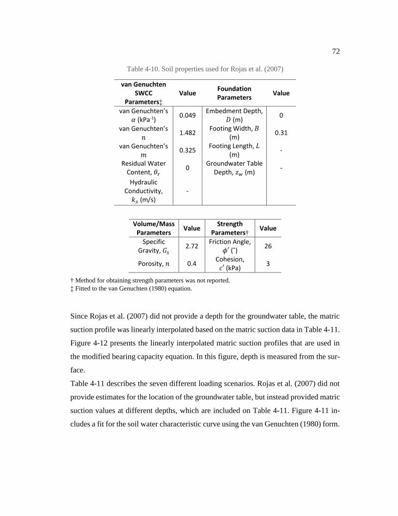
72
Table 4-10. Soil properties used for Rojas et al. (2007)
van Genuchten SWCC
Parameters‡ Value
Foundation Parameters
Value
van Genuchten’s 𝛼 (kPa-1)
0.049 Embedment Depth,
𝐷 (m) 0
van Genuchten’s 𝑛
1.482 Footing Width, 𝐵
(m) 0.31
van Genuchten’s 𝑚
0.325 Footing Length, 𝐿
(m) -
Residual Water Content, 𝜃𝑟
0 Groundwater Table
Depth, 𝑧𝑤 (m) -
Hydraulic Conductivity,
𝑘𝑠 (m/s) -
Volume/Mass Parameters
Value Strength
Parameters† Value
Specific Gravity, 𝐺𝑠
2.72 Friction Angle,
𝜙′ (˚) 26
Porosity, 𝑛 0.4 Cohesion,
𝑐′ (kPa) 3
† Method for obtaining strength parameters was not reported.
‡ Fitted to the van Genuchten (1980) equation.
Since Rojas et al. (2007) did not provide a depth for the groundwater table, the matric
suction profile was linearly interpolated based on the matric suction data in Table 4-11.
Figure 4-12 presents the linearly interpolated matric suction profiles that are used in
the modified bearing capacity equation. In this figure, depth is measured from the sur-
face.
Table 4-11 describes the seven different loading scenarios. Rojas et al. (2007) did not
provide estimates for the location of the groundwater table, but instead provided matric
suction values at different depths, which are included on Table 4-11. Figure 4-11 in-
cludes a fit for the soil water characteristic curve using the van Genuchten (1980) form.

73
Figure 4-11. Fitted SWCC for the Rojas et al. (2007) data.
Table 4-11. Matric suction from tests and maximum bearing capacity from hyperbolic fit for
Rojas et al. data (2007).
Test No.
Matric Suction 𝝍 [kPa] at Depth [m] 𝒒𝒖𝒍𝒕
[kPa] 0.1 0.3 0.6 0.9
S1 0 0 0 0 450
S2 0 3 0 0 376
U1 10 4 13 0 552
U2 48 38 15 0 671
U3 56 46 4 0 961
U4 60 53 6 4 980
U5 63 57 11 0 1112
0.01 0.1 1 10 100 1 103
1 104
0
0.1
0.2
0.3
0.4
Data from Pressure Plates
Data from Tensionmeter
Fitted VG Equation
Suction [kPa]
Vo
lum
etri
c W
ate
r C
on
ten
t [%
]

74
Figure 4-12. Linearly interpolated matric suction profile for Rojas et al. (2007) data
The modified bearing capacity calculations accounting for partial saturation through
these matric suction profiles results in the values presented in Figure 4-13.
Figure 4-13. Comparison of calculated qult for the Rojas et al. (2007) data using the modified
and unmodified bearing capacity equation.
0 0.2 0.4 0.6 0.8 1
20
40
60
80
Depth [m]
Mat
ric
Su
ctio
n [
kP
a]
0
300
600
900
1200
1500
0 300 600 900 1200 1500
Cal
cula
ted
Bea
rin
g C
apac
ity
[kP
a]
Measured Bearing Capacity [kPa]
ModifiedApproach
ConventionalApproach
S1
U1
S2
U2
U1
U3
U1
U4
U1
U5
U1
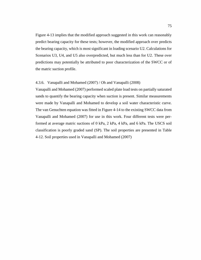
75
Figure 4-13 implies that the modified approach suggested in this work can reasonably
predict bearing capacity for these tests; however, the modified approach over predicts
the bearing capacity, which is most significant in loading scenario U2. Calculations for
Scenarios U3, U4, and U5 also overpredicted, but much less than for U2. These over
predictions may potentially be attributed to poor characterization of the SWCC or of
the matric suction profile.
4.3.6. Vanapalli and Mohamed (2007) / Oh and Vanapalli (2008)
Vanapalli and Mohamed (2007) performed scaled plate load tests on partially saturated
sands to quantify the bearing capacity when suction is present. Similar measurements
were made by Vanapalli and Mohamed to develop a soil water characteristic curve.
The van Genuchten equation was fitted in Figure 4-14 to the existing SWCC data from
Vanapalli and Mohamed (2007) for use in this work. Four different tests were per-
formed at average matric suctions of 0 kPa, 2 kPa, 4 kPa, and 6 kPa. The USCS soil
classification is poorly graded sand (SP). The soil properties are presented in Table
4-12. Soil properties used in Vanapalli and Mohamed (2007)
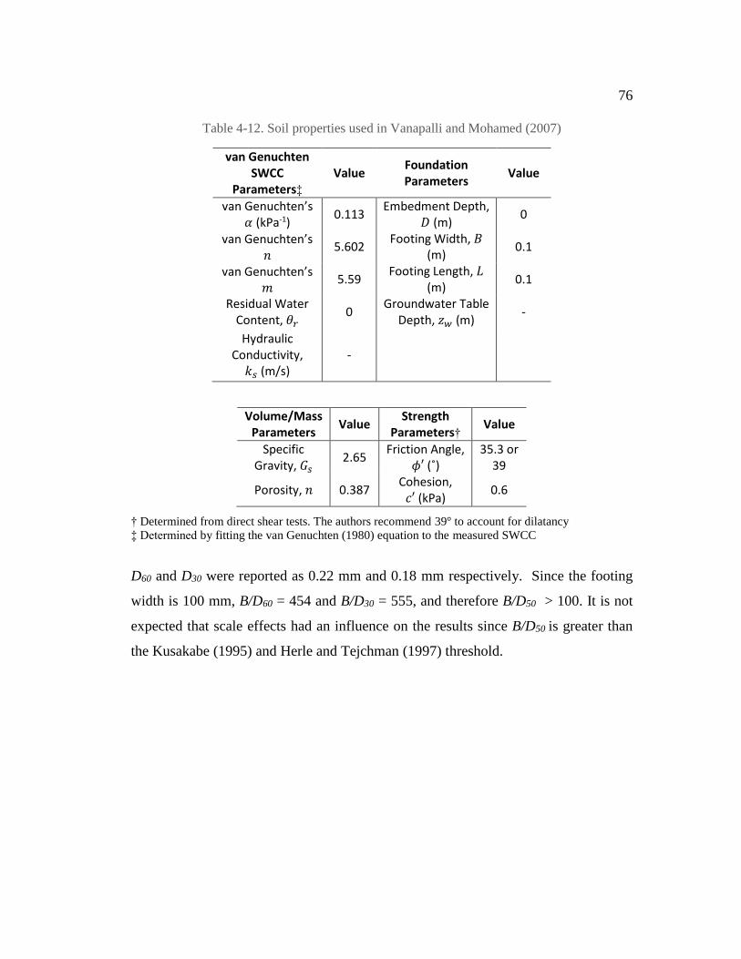
76
Table 4-12. Soil properties used in Vanapalli and Mohamed (2007)
van Genuchten SWCC
Parameters‡ Value
Foundation Parameters
Value
van Genuchten’s 𝛼 (kPa-1)
0.113 Embedment Depth,
𝐷 (m) 0
van Genuchten’s 𝑛
5.602 Footing Width, 𝐵
(m) 0.1
van Genuchten’s 𝑚
5.59 Footing Length, 𝐿
(m) 0.1
Residual Water Content, 𝜃𝑟
0 Groundwater Table
Depth, 𝑧𝑤 (m) -
Hydraulic Conductivity,
𝑘𝑠 (m/s) -
Volume/Mass Parameters
Value Strength
Parameters† Value
Specific Gravity, 𝐺𝑠
2.65 Friction Angle,
𝜙′ (˚) 35.3 or
39
Porosity, 𝑛 0.387 Cohesion,
𝑐′ (kPa) 0.6
† Determined from direct shear tests. The authors recommend 39° to account for dilatancy
‡ Determined by fitting the van Genuchten (1980) equation to the measured SWCC
D60 and D30 were reported as 0.22 mm and 0.18 mm respectively. Since the footing
width is 100 mm, B/D60 = 454 and B/D30 = 555, and therefore B/D50 > 100. It is not
expected that scale effects had an influence on the results since B/D50 is greater than
the Kusakabe (1995) and Herle and Tejchman (1997) threshold.

77
Figure 4-14. Fitted SWCC using van Genuchten (1980) (after Vanapalli and Mohamed 2007)
In this work, measurements of matric suction were made at the bottom of the foundation
and at a depth of 1.5B from the bottom of the foundation. The reported suction was
then the average of these two values. An equivalent ground water could be determined
from Eq. 4-1 assuming matric suction increases linearly above the groundwater table.
This equation was developed to match the provided average matric suctions since the
framework presented in this work uses groundwater table depths instead.
𝜓 =
1
2(𝑧𝑤𝛾𝑤 + (𝑧𝑤 − 1.5𝐵)𝛾𝑤) 4-1
where 𝜓 is the matric suction, 𝑧𝑤 is the depth of the groundwater table, 𝐵 is the footing
width, and 𝛾𝑤 is the unit weight of water. Solving for depth of the ground water table:
𝑧𝑤 =𝜓
𝛾𝑤+ 0.75𝐵 if 𝜓 > 0.75𝐵𝛾𝑤 4-2
𝑧𝑤 =2𝜓
𝛾𝑤 if 𝜓 < 0.75𝐵𝛾𝑤 4-3
For average matric suctions of 0 kPa, 2 kPa, 4 kPa, and 6 kPa the equivalent ground-
water table depth is 0 m, 0.279 m, 0.483 m, and 0.687 m.
0 2 4 6 8 10
20
40
60
80
100
Suction [kPa]
Satu
rati
on
[%
]

78
Figure 4-15 compares the predicted bearing capacity to the measured bearing capacity
using a friction angle of 𝜙′ = 39° and the groundwater table depths described previ-
ously. The bearing capacity was calculated using both the modified approach presented
in this work and the conventional approach. Vanapalli and Mohamed (2007) proposed
a closed-formed solution to the bearing capacity of shallow foundations in Eq. 4-4
which is also compared in this figure. This equation is discussed in Section 2.1.3.
𝑞𝑢𝑙𝑡 = [𝑐′ + (𝑢𝑎 − 𝑢𝑤)𝑏(1 − 𝑆𝜓) tan 𝜙′ + (𝑢𝑎 −
𝑢𝑤)𝐴𝑉𝑅𝑆𝜓 tan 𝜙′] 𝑁𝑐 [1 + (𝑁𝑞
𝑁𝑐) (
𝐵
𝐿)] + 0.5𝐵𝛾𝑁𝛾 [1 − 0.4
𝐵
𝐿]
4-4
The modified approach and the equation proposed by Vanapalli and Mohamed (2007)
show good agreement with the measured bearing capacity.
Figure 4-15. Comparison of actual bearing capacity to predictions from this work and
Vanapalli and Mohamed (2007)
Figure 4-16 compares the bearing capacity of the model shallow foundation to the av-
erage suction applied at D and D + B. Interestingly, the peak bearing capacity calcu-
lated using the modified approach proposed herein and the measured bearing capacities
0
200
400
600
800
1000
0 200 400 600 800 1000
Cal
cula
ted
Be
arin
g C
apac
ity
[kP
a]
Measured Bearing Capacity [kPa]
This Work
Vanapalli andMohamed (2007)ConventionalApproach

79
from Vanapalli and Mohamed (2007) are essentially the same. The bearing capacity
predicted in this work quickly reduces after 5 kPa. This is quite different to the work
of Vanapalli and Mohamed, who predict a slower decline in strength with an increase
in suction.
Figure 4-16. Bearing capacity vs. variation in average matric suction from this work and
Vanapalli and Mohamed (2007)
The bearing capacity profile calculated from the proposed modified approach shows a
peak at approximately 5 kPa followed by a dramatic decrease in bearing capacity after
6 kPa, converging to the conventional approach at higher suctions. The bearing capac-
ity profile calculated from the Vanapalli and Mohamed (2007) equation shows an in-
crease in bearing capacity until 6 kPa followed by a shallow decrease in bearing capac-
ity at higher suctions. The SWCC in Figure 4-14 shows an air-entry suction of approx-
imately 4 kPa followed by rapid desaturation, therefore the profile predicted by this
current work is more consistent with the SWCC than that predicted by Vanapalli and
Mohamed (2007).
0
300
600
900
1200
1500
0 2 4 6 8 10
Be
arin
g C
apac
ity
[kP
a]
Matric Suction [kPa]
This Work
Vanapalli and Mohamed (2007)
Conventional Approach
Measured Bearing Capacity

80
4.3.7. Vanapalli and Mohamed (2013)
Vanapalli and Mohamed (2013) used the same soil as in Vanapalli and Mohamed
(2007); refer to Table 4-12 for the soil properties. The difference between this and the
previous work was the use of a larger 150 mm plate embedded at depths of 0 mm and
150 mm. The surface plate was loaded at average suction stresses of 0 kPa, 2 kPa, 4
kPa, and 6 kPa, which can be represented with groundwater table depths of 0 m, 0.317
m, 0.521 m, and 0.725 m as calculated with Eqs. 4-1, 4-2 and 4-3. The embedded plate
was tested at 0 kPa, 2 kPa, and 6 kPa, which can be represented with groundwater table
depths of 0 m, 0.317 m, and 0.725 m. The authors recommend that when the footing is
embedded, a friction angle of 35.3° should be used instead of 39° to account for a re-
duction in dilation.
Figure 4-17. Comparison of measured and predicted bearing capacity for 150 mm surface
plate for Vanapalli and Mohamed (2013)
Figure 4-17 compares measured bearing capacity to the bearing capacity calculated by
the modified approach, the Vanapalli and Mohamed approach, and the conventional
approach. Both the modified and the Vanapalli and Mohamed approach show close
0
200
400
600
800
1000
0 200 400 600 800 1000
Cal
cula
ted
Be
arin
g C
apac
ity
[kP
a]
Measured Capacity [kPa]
This Work
Vanapalli andMohamed (2013)ConventionalApproach
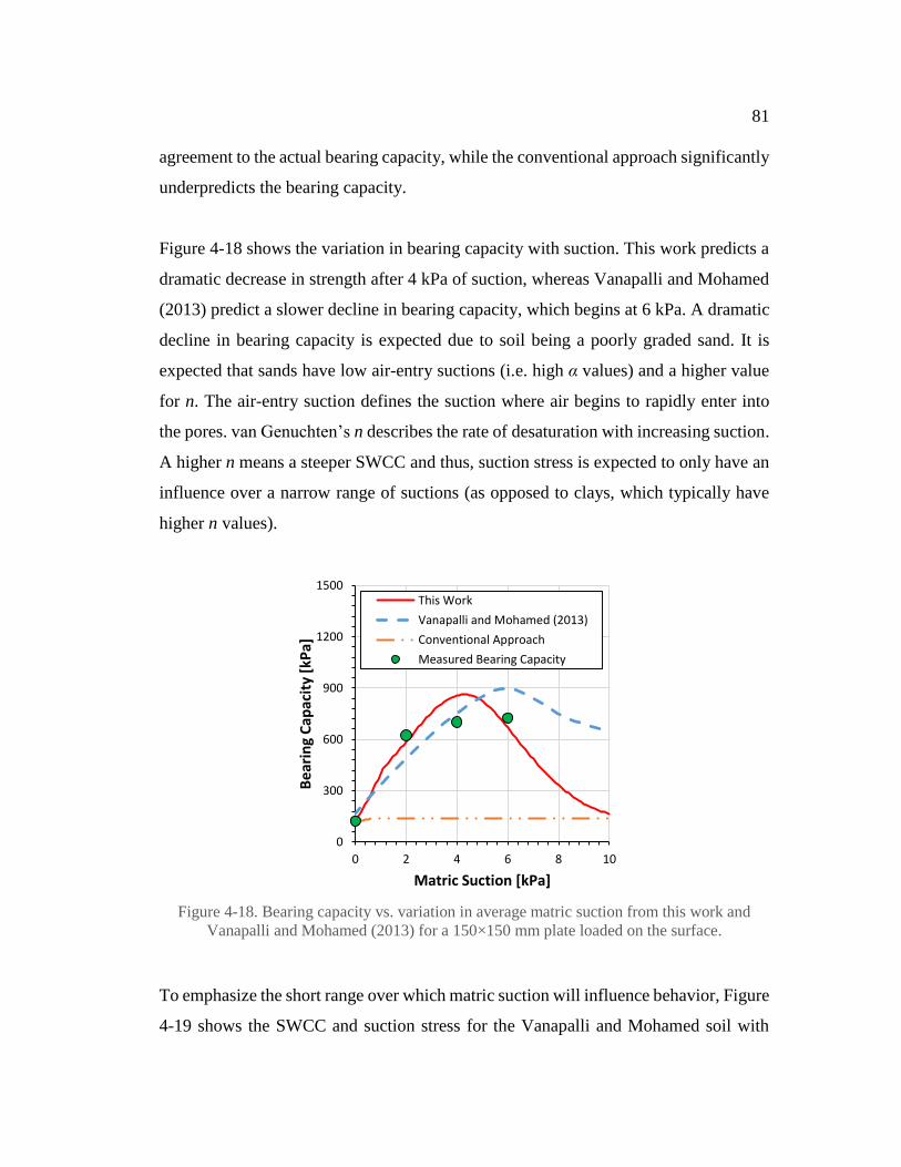
81
agreement to the actual bearing capacity, while the conventional approach significantly
underpredicts the bearing capacity.
Figure 4-18 shows the variation in bearing capacity with suction. This work predicts a
dramatic decrease in strength after 4 kPa of suction, whereas Vanapalli and Mohamed
(2013) predict a slower decline in bearing capacity, which begins at 6 kPa. A dramatic
decline in bearing capacity is expected due to soil being a poorly graded sand. It is
expected that sands have low air-entry suctions (i.e. high α values) and a higher value
for n. The air-entry suction defines the suction where air begins to rapidly enter into
the pores. van Genuchten’s n describes the rate of desaturation with increasing suction.
A higher n means a steeper SWCC and thus, suction stress is expected to only have an
influence over a narrow range of suctions (as opposed to clays, which typically have
higher n values).
Figure 4-18. Bearing capacity vs. variation in average matric suction from this work and
Vanapalli and Mohamed (2013) for a 150×150 mm plate loaded on the surface.
To emphasize the short range over which matric suction will influence behavior, Figure
4-19 shows the SWCC and suction stress for the Vanapalli and Mohamed soil with
0
300
600
900
1200
1500
0 2 4 6 8 10
Bea
rin
g C
apac
ity
[kP
a]
Matric Suction [kPa]
This Work
Vanapalli and Mohamed (2013)
Conventional Approach
Measured Bearing Capacity

82
respect to distance above the groundwater table. As stated previously, water content
decreases rapidly above the groundwater table, resulting in negligible suction stresses
at suctions greater than 4 or 5 kPa. If the groundwater table was at a depth of 1 m
(approximately 10 kPa matric suction) there should be little suction stress acting on the
failure surface.
Figure 4-19. SWCC and suction stress profile for Vanapalli and Mohamed (2013) soil.
The second set of testing Vanapalli and Mohamed (2013) performed was on plates
embedded at a depth of 150 mm. Since the plates were embedded, the authors argued
that effects due to dilation could be ignored. However, the confining stress associated
with 150 mm of overburden is quite small; thus, in this work, both the original value
of 𝜙′ and the recommended scaled value of 1.1𝜙′ are considered to account for the
dilation of the densely packed sand. Figure 4-20 compares the measured bearing ca-
pacity for the embedded plate against the modified approach for friction angles of 35.3˚
and 39˚ and against the Vanapalli and Mohamed approach. Figure 4-21 presents the
bearing capacity profile from these two approaches and the measured bearing capacity.
0 0.1 0.2 0.3
0.5
1
1.5
2
Gravimetric Water Content
Dis
tan
ce A
bo
ve G
WT
[m
]
0 1 2 3 4 5
0.5
1
1.5
2
Suction Stress [kPa]
Dis
tan
ce A
bo
ve G
WT
[m
]

83
Figure 4-20. Comparison of measured and calculated bearing capacity for 150 mm embedded
plate for Vanapalli and Mohamed (2013)
This work shows that friction angles of 39° and 35.3° bracket the measured bearing
capacity. This may imply that the assumption that dilation can be ignored for embedded
foundations is not valid, but rather, that dilation is suppressed, which is consistent with
conventional shear strength theory. The equation proposed by Vanapalli and Mohamed
show good agreement to the measured data.
0
300
600
900
1200
1500
0 300 600 900 1200 1500
Cal
cula
ted
Bea
rin
g C
apac
ity
[kP
a]
Measured Bearing Capacity [kPa]
This Work (Friction = 35.3)
This Work (Friction = 39.0)
Vanapalli and Mohamed (2013)

84
Figure 4-21. Bearing capacity vs. variation in average matric suction from this work and
Vanapalli and Mohamed (2013) for a 150×150 mm plate embedded 150 mm.
4.3.8. Wuttke et al. (2013)
Wuttke et al. (2013) performed scaled load tests on shallow strip foundations. In this
work, the soil was desaturated via suction in order to replicate the suction stress that
occurs in-situ due to the presence of a groundwater table. The soil used in this work is
Hostun sand, which has a USCS classification of poorly graded sand (SP). The SWCC
was determined experimentally, so no prediction is required. The fitted SWCC is
shown in Figure 4-22. In this work, the plate is loaded over partially saturated soil and
suctions is measured at various depths. The sand specimen is saturated from the bottom.
The properties of Hostun sand are presented in Table 4-13.
0
500
1000
1500
2000
0 2 4 6 8 10
Bea
rin
g C
apac
ity
[kP
a]
Matric Suction [kPa]
This Work (Friction = 35.3)This Work (Friction = 39.0)Vanapalli and Mohamed (2013)Measured Bearing Capacity

85
Table 4-13. Soil properties for Hostun sand (Wuttke et al. 2007)
van Genuchten Drying SWCC Parameters‡
Value van Genuchten Wetting SWCC
Parameters Value
Foundation Parameters
Value
van Genuchten’s 𝛼 (kPa-1)
0.46 van Genuchten’s
𝛼 (kPa-1) 0.906
Embedment Depth, 𝐷 (m)
0
van Genuchten’s 𝑛
14.35 van Genuchten’s
𝑛 3.411
Footing Width, 𝐵 (m)
0.079
van Genuchten’s 𝑚
0.278 van Genuchten’s
𝑚 0.701
Footing Length, 𝐿 (m)
0.477
Residual Water Content, 𝜃𝑟
0.017 Residual Water
Content, 𝜃𝑟 0.017
Groundwater Table Depth, 𝑧𝑤 (m)
-
Hydraulic Conductivity,
𝑘𝑠 (m/s) -
Hydraulic Conductivity,
𝑘𝑠 (m/s) -
Volume/Mass Parameters
Value Strength
Parameters† Value
Specific Gravity, 𝐺𝑠
2.65 Friction Angle,
𝜙′ (˚) 46.7
Porosity, 𝑛 0.395 Cohesion,
𝑐′ (kPa) -
† Determined under plane-strain loading conditions using a double-wall cell
‡ Determined by fitting the van Genuchten (1980) equation to the measured SWCC
Kusakabe (1995) and Herle and Tejchman (1997) recommend a threshold of 𝐵/𝐷50 ≥
100 to avoid particle size affects. Hostun sand has 𝐷50 = 0.35 mm while the scaled
footing has a width of 𝐵 = 79 mm. 𝐵/𝐷50 = 226 which is over twice the recom-
mended value, implying that scaled effects should be small.

86
Figure 4-22. Soil water characteristic curve for Hostun sand (after Wuttke et al. 2013)
In this work, measurements of matric suction were made at the bottom of the foundation
and at a depth of 1.5B from the bottom of the foundation. The reported suction was
then the average of these two values. This is similar to the work done by Vanapalli and
Mohamed (2007). Wuttke et al. (2013) made measurements at 2 kPa, 3 kPa, 4 kPa,
completely dry, and completely saturated. This corresponds to groundwater tables
depths of 263mm, 365mm, 467mm, very deep (approximated as 1000mm), and 0mm.
The bearing capacity profile was calculated using the modified approach and the con-
ventional bearing capacity equation in Figure 4-23. In Figure 4-24, the measured bear-
ing capacity was compared to values calculated from the modified and conventional
approach. For the modified approach, two separate calculations were made using van
Genuchten properties for the wetting and drying curves shown in Figure 4-22.
0.1 1 10 1000
10
20
30
40
Wetting Curve
Drying Curve
Suction [kPa]
Vo
lum
etri
c W
ater
Co
nte
nt
[%]

87
Figure 4-23. Calculated and measured bearing capacities compared to the average matric suc-
tion at D and D + B.
Figure 4-23 shows that the measured bearing capacity was generally between both the
wetting and drying curve. The calculated bearing capacity using both the wetting and
drying soil water characteristic curves performed well compared to the measured bear-
ing capacity and compared to the conventional bearing capacity equation, as in Figure
4-24.
0
300
600
900
1200
0 2 4 6
Cal
cula
ted
Bea
rin
g C
apac
ity
[kP
a]
Matric suction [kPa]
Wetting SWCC
Drying SWCC
Conventional Approach
Measured Bearing Capacity

88
Figure 4-24. Comparison of actual bearing capacity to predictions from the conventional and
modified approach for Wuttke et al. (2013)
4.4. Summary and Discussion
This chapter provided validation for the modified bearing capacity equation proposed
in this work. The comparative study in Section 4.3 included several load tests con-
ducted on both model and full-scaled shallow foundations. Bearing capacities were cal-
culated using the modified bearing capacity equation and the conventional equation.
Figure 4-25 summarizes the comparative study in Section 4.3, comparing the measure
bearing capacity for the load tests in this section against the predicted bearing capacity
using the modified and conventional approach. Trendlines were fitted to the data for
comparison against the 1:1 line. Data from Larsson (1997) was not included in this
figure since the groundwater table depth was not provided in this work.
0
200
400
600
800
0 200 400 600 800
Cal
cula
ted
Bea
rin
g C
apac
ity
[kP
a]
Measured Bearing Capacity [kPa]
WettingSWCCDrainedSWCCConventionalApproach

89
Figure 4-25. Measured bearing capacity vs. predicted bearing capacity for database of load
tests in Chapter 4.
The linear trendline fitted to the modified approach shows closer agreement to the 1:1
line than the conventional approach. The conventional bearing capacity equation will
generally underpredict bearing capacity. The slope of the trendline for modified ap-
proach is 0.93 while the slope for the conventional approach is 0.43. Using linear re-
gression against the 1:1 line gives a coefficient of determination, R2, of 0.81 for the
modified approach and -2 for the conventional. The closer the coefficient of determi-
nation is to 1, the better the fit. A negative R2 implies that the conventional approach
does not at all correlate with the measured bearing capacity.
In summary, this chapter shows that the conventional bearing capacity equation will
generally underpredict the bearing capacity except at lower bearing capacities (which
the majority are saturated load tests). The modified bearing capacity equation shows
close agreement to the measured bearing capacity data presented in this section, vali-
dating the approach used in this work. Suction stresses (not matric suction) in partially
saturated soils will have the tendency to increase soil strength, increasing the bearing
capacity.
0
600
1200
1800
2400
0 600 1200 1800 2400
Cal
cula
ted
Bea
rin
g C
apac
ity
[kP
a]
Measured Bearing Capacity [kPa]
Modified
Conventional
Linear (Modified)
Linear (Conventional)

90
5. Parametric Studies
5.1. Outline of Parametric Studies
In this section, shallow and deep foundation performance will be evaluated with respect
to varying soil parameters such as 𝜙′, 𝜃𝑟, 𝜃𝑠, 𝛼, 𝑛, 𝑚, and 𝑘𝑠 where all terms are as
previously defined. Further considerations will also be made to foundation shape – such
as footing width 𝐵 and embedment depth 𝐷, groundwater table depth 𝑧𝑤, and variation
to water infiltration 𝑞. In this study, considerations will not be made to the cohesion 𝑐′,
specific gravity 𝐺𝑠, and footing length 𝐿 since these parameters will not affect the foun-
dation performance differently in unsaturated soils than in saturated soils. The soil
types that will be selected in this study are sand, silt, and clay. These three soil types
serve as the extremes (as in the sand and clay) and average (silt) for typical soil water
characteristic curves.
Section 5.2 will present the soil properties that correspond to the theoretical sand, silt,
and clay that are used in this parametric study. Section 5.3 will cover parametric studies
on shallow foundations. Section 5.4 will cover parametric studies on deep foundations,
presenting only a discussion on shaft resistance. Section 5.5 will cover Monte Carlo
analyses for shallow foundation bearing capacity using Carsel and Parrish (1988) to
calculate appropriate realizations for unsaturated soil properties. Chapter 5 will be
concluded with a discussion in Section 5.6.
5.2. Soils Parameters Used in Parametric Study
The soil types that will be used in this study are sand, silt, and clay. 𝛼 generally varies
by a magnitude between sand, silt and clay. The selection of 𝛼 = 1.0, 0.1, and 0.01
kPa-1 for sand, silt, and clay are simple values that describe the general ranges of 𝛼
between these three soil types. van Genuchten’s fitting parameter 𝑛 is mathematically
limited to being greater than 1.0, so for clays, a value of 1.1 was selected. For theoret-
ical silt and sand, 𝑛 values of 1.5 and 3.0 will be used. These value have been selected

91
to describe the range at which 𝛼 and 𝑛 vary between all three soil types. Hydraulic
conductivity between sand, silt, and clay can vary by a magnitude or more, thus, 𝑘𝑠 =
10-5, 10-6, and 10-7 m/s respectively are selected as typical values. 𝜃𝑠 = 0.4 and 𝜃𝑟 =
0.06 are used to describe the saturated and residual water contents, respectively. The
below table summarizes the hydraulic properties used in the following parametric stud-
ies for each of theoretical sand, silt, and clay.
Table 5-1. Soil properties used in this parametric study
𝜶 (𝐤𝐏𝐚−𝟏) 𝒏 𝒌𝒔 (𝐦/𝐬) 𝜽𝒔 𝜽𝒓
Clay 0.01 1.1 10-7 0.4 0.06
Silt 0.10 1.5 10-6 0.4 0.06
Sand 1.00 3.0 10-5 0.4 0.06
In this study, the bearing capacity of a shallow foundation and the 𝛽-method for deep
foundations will be evaluated with the ranges of variables proposed in Table 5-1. Fur-
ther, the typical 𝜃𝑠 value will be taken as 0.4, but will be studied at 0.35 and 0.45.
Likewise, the typical 𝜃𝑟 value will be taken as 0.06, but will be studied at 0.02 and 0.1.
Van Genuchten’s 𝑚 will be set equal to 𝑚 = 1 − 1/𝑛 (Mualem 1976; van Genuchten
1980). For all three soil types 𝑐′ = 0 kPa, and 𝐺𝑠 = 2.65. 𝜙′ will be studied at 25°,
30°, and 35°. When the effects of fluid flux are studied, values ranging from 𝑞 =
−3.14 × 10⁻⁸ m/s to 1.15 × 10⁻⁸ m/s will be used. This range is recommended by
Lu and Likos (2004) as representative flux values.
Carsel and Parrish (1988) determined average values for unsaturated soil properties
including 𝜃𝑠, 𝜃𝑟, 𝛼 and 𝑛, as discussed in Section 2.3.8. Typical soil water characteristic
curves have been plotted from these mean values listed in Table 2-1 using the van
Genuchten (1980) equation:
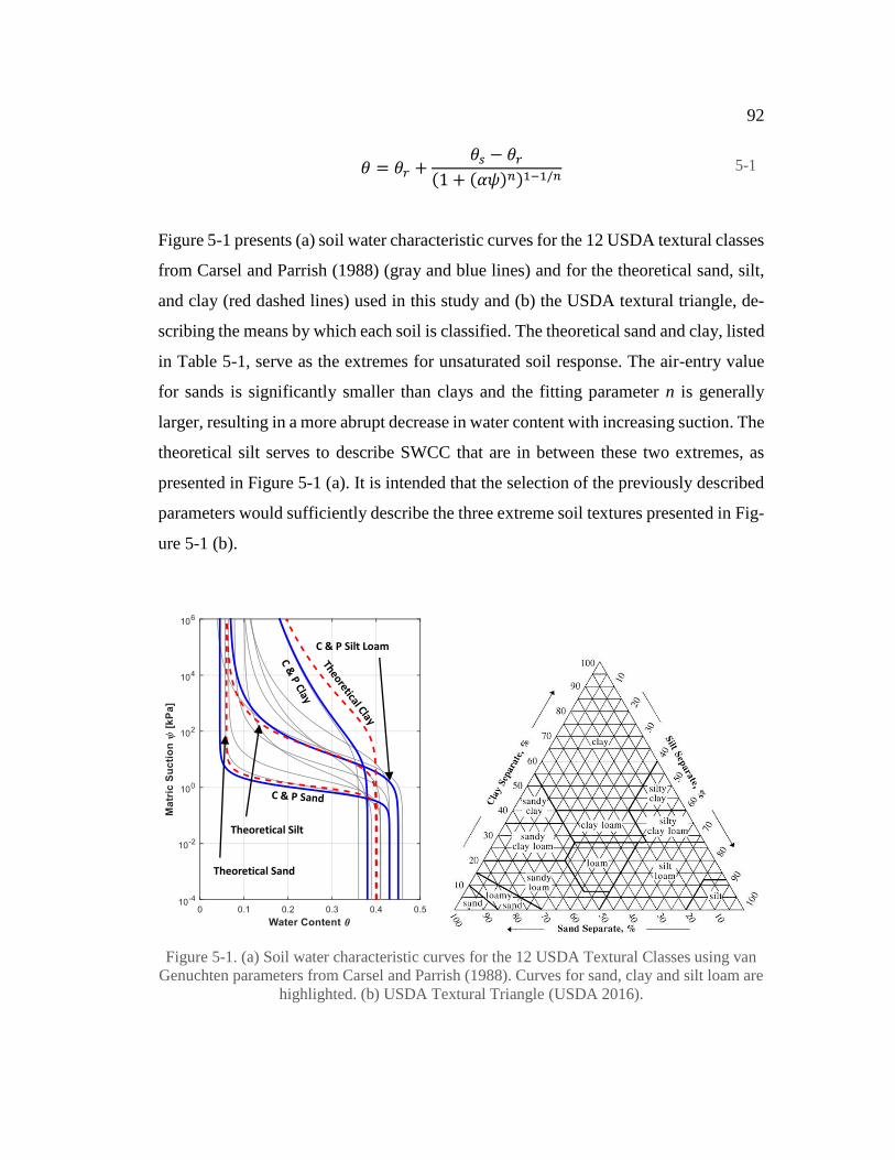
92
𝜃 = 𝜃𝑟 +
𝜃𝑠 − 𝜃𝑟
(1 + (𝛼𝜓)𝑛)1−1/𝑛 5-1
Figure 5-1 presents (a) soil water characteristic curves for the 12 USDA textural classes
from Carsel and Parrish (1988) (gray and blue lines) and for the theoretical sand, silt,
and clay (red dashed lines) used in this study and (b) the USDA textural triangle, de-
scribing the means by which each soil is classified. The theoretical sand and clay, listed
in Table 5-1, serve as the extremes for unsaturated soil response. The air-entry value
for sands is significantly smaller than clays and the fitting parameter n is generally
larger, resulting in a more abrupt decrease in water content with increasing suction. The
theoretical silt serves to describe SWCC that are in between these two extremes, as
presented in Figure 5-1 (a). It is intended that the selection of the previously described
parameters would sufficiently describe the three extreme soil textures presented in Fig-
ure 5-1 (b).
Figure 5-1. (a) Soil water characteristic curves for the 12 USDA Textural Classes using van
Genuchten parameters from Carsel and Parrish (1988). Curves for sand, clay and silt loam are
highlighted. (b) USDA Textural Triangle (USDA 2016).
C & P Silt Loam
Theoretical Sand
Theoretical Silt

93
The soil water characteristic curves for sand, silt loam, and clay noted Carsel and Par-
rish (1988) as they compare relatively well with the values that are used for this study.
The theoretical soils used in this study, as shown with the dashed lines, bracket the
ranges of SWCCs described in Carsel and Parrish (1988).
5.3. Parametric Studies on Shallow Foundations
The shallow foundation portion of the parametric study will be composed of founda-
tions that have a footing width 𝐵 = 1 m. All other footing shape parameters and water
depth will be normalized to this value with the exception of the footing length, 𝐿, which
is considered to be very long (i.e. a strip footing). The depth of embedment will be
studied at four different depths: 𝐷 = 0, 𝐵/2, 𝐵, and 3𝐵/2. The variation of the ground-
water table will be set to 𝑧𝑤 = 𝐷 to 𝑧𝑤 = 𝐷 + 4𝐵.
5.3.1. Shallow Foundation Bearing Capacity Profiles
The first set of analyses in the shallow foundation parametric study calculate bearing
capacity as a function of the groundwater table depth. The deeper the groundwater ta-
ble, the higher the matric suction is near the soil surface. A plot comparing bearing
capacity vs. depth of the groundwater table will subsequently be called the bearing
capacity profile. Evaluating the influence of matric suction on bearing capacity is the
focus of this research, so beginning the parametric study with these bearing capacity
profiles is important. Bearing capacity will be calculated according to the methodology
described for shallow foundations in Section 3.2. For each figure, one input parameter
will be varied to assess its effect on bearing capacity. For these figures, zw will be eval-
uated to a depth of 4 m, which is deeper than the foundation stress bulb D + B.
The first figure, Figure 5-2, presents the influence of friction angle on partially satu-
rated soils. Three different friction angles, 𝜙′ = 25°, 30°, and 35° are assessed for the
theoretical sand, silt, and clay with an embedment depth D = 0 m. Note that in Figure
5-2 and in the subsequent figures of bearing capacity profiles, the y-axis will not be

94
plotted to the same scale. This is because the theoretical suction stresses in clays are
large, resulting in high bearing capacities.
Figure 5-2. Shallow foundation bearing capacity profile of clay, silt, and sand at varying
friction angles. Note changing ordinate across figures.
Figure 5-2 demonstrates the large influence suction stress have on fine-grained soils.
The more fine a soil is (lower 𝑛 and 𝛼), the greater the influence generally is. With the
same friction angle, clays see a bearing capacities that are significantly greater than for
sands. Since the value predicted for clays and silts are large, it is important to note that
these are theoretical predictions, uncalibrated to physical measurements. As expected,
with an increase in friction angle, the strength increases as well, although it is a non-
linear increase. In subsequent figures, 𝜙′ will be held at 30°.
0
500
1000
1500
2000
2500
3000
0 1 2 3 4
Bea
rin
g C
apac
ity
[kP
a]
GWT Depth [m]
Clay, n = 1.1α = 0.01 kPa-1
0
400
800
1200
1600
2000
0 1 2 3 4
Bea
rin
g C
apac
ity
[kP
a]GWT Depth [m]
Silt, n = 1.5α = 0.1 kPa-1
0
100
200
300
400
500
600
0 1 2 3 4
Be
arin
g C
apac
ity
[kP
a]
GWT Depth [m]
Sand, n = 3.0α = 1.0 kPa-1
050010001500200025003000
-2 3
φ' = 25°
φ' = 30°
φ' = 35°

95
Figure 5-3 presents the influence of foundation embedment depth on the bearing ca-
pacity profile in partially saturated soils. The 1 m footing is embedded D = 0, B/2, B,
and 3B/2 and is assessed for theoretical sand, silt, and clay.
Figure 5-3. Shallow foundation bearing capacity vs. zgwt - D for clay, silt, and sand at varying
depths of embedment. Note changing ordinate across figures.
Figure 5-3 compares bearing capacity profile to embedment depth. The embedment
depth is subtracted from the groundwater table depth so that the plots would all begin
at 0. This figure shows that increasing the depth of embedment of a shallow foundation
in unsaturated soils will only increase the bearing capacity by a constant value for all
ranges of zgwt – D. The increase in bearing capacity can be attributed to the overburden
0
500
1000
1500
2000
2500
3000
0 1 2 3 4
Be
arin
g C
apac
ity
[kP
a]
zgwt - D [m]
Clay, n = 1.1α = 0.01 kPa-1
0
400
800
1200
1600
2000
0 1 2 3 4
Be
arin
g C
apac
ity
[kP
a]
zgwt - D [m]
Silt, n = 1.5α = 0.1 kPa-1
0
300
600
900
1200
0 1 2 3 4
Be
arin
g C
apac
ity
[kP
a]
zgwt - D [m]
Sand, n = 3.0α = 1.0 kPa-1
050010001500200025003000
-2 3
D = 0
D = B/2
D = B
D = 3B/2

96
term in the bearing capacity equation, which accounts for suction and normal stresses,
and the depth factors introduced by Hansen (1970).
Similarly, the data in Figure 5-3 can be plotted against groundwater depth only. This is
done in Figure 5-4.
Figure 5-4. Shallow foundation bearing capacity vs. groundwater table depth for clay, silt,
and sand at varying depths of embedment. Note changing ordinate across figures.
Figure 5-4 shows another interesting trend for embedded foundations in partially satu-
rated soils. While the previous figure shows that increasing depth of embedment in-
creases bearing capacity by a constant, this does not prevent shallower foundations to
0
500
1000
1500
2000
2500
0 1 2 3 4
Be
arin
g C
apac
ity
[kP
a]
zgwt [m]
Clay, n = 1.1α = 0.01 kPa-1
0
400
800
1200
1600
0 1 2 3 4
Be
arin
g C
apac
ity
[kP
a]
zgwt [m]
Silt, n = 1.5α = 0.1 kPa-1
0
200
400
600
800
1000
0 1 2 3 4
Be
arin
g C
apac
ity
[kP
a]
zgwt [m]
Sand, n = 3.0α = 1.0 kPa-1
05001000150020002500
-2 3
D = 0
D = B/2
D = B
D = 3B/2

97
have a greater bearing capacity. This is observed in a silt, where D = 0 exceeds D = B/2
for a portion of the figure.
Another component of this research is to assess the influence of infiltration and evap-
oration on bearing capacity. The matric suction profile and its implementation in cal-
culating bearing capacity are discussed in Sections 2.3.6 and 3.2.1. Figure 5-5 plots the
bearing capacity profile at three different rates of flux, q = -3.14E-8 m/s (which is in-
filtration), q = 0 (which is no flow), and q = 1.15E-8 m/s (which is evaporation). This
is done for the theoretical sand, silt, and clay.
Figure 5-5. Shallow foundation bearing capacity profile of clay, silt, and sand with varying
rates of flux. Note changing ordinate across figures.
0
500
1000
1500
2000
0 1 2 3 4
Be
arin
g C
apac
ity
[kP
a]
GWT Depth [m]
Clay, ks = 10-7 m/s
0
400
800
1200
0 1 2 3 4
Be
arin
g C
apac
ity
[kP
a]
GWT Depth [m]
Silt, ks = 10-6 m/s
0
50
100
150
200
250
0 1 2 3 4
Bea
rin
g C
apac
ity
[kP
a]
GWT Depth [m]
Sand, ks = 10-5 m/s
0500100015002000
-2 3
q = -3.14E-8 m/s
q = 0 m/s
q = 1.15E-8 m/s

98
Two behaviors can be distinguished from these plots: (1) in the theoretical silt and clay,
bearing capacity increases with evaporation; and (2) in sand, bearing capacity increases
with infiltration. The explanation for this discrepancy is that in sands suction stresses
are very small (e.g., Lu et al. 2010) and at net zero flow or evaporation the pores are
likely at or near residual saturation, implying that suction stresses are low. When infil-
tration occurs in sands, the pores become filled with water increasing the average unit
weight and suction stress, thus increasing the bearing capacity. Alternatively, in silts
and clays the suction stresses are much higher, allowing for water to be retained in the
pores. Infiltration in silts and clays would cause the suction stress to decrease and there-
fore the bearing capacity as well.
Figure 5-6 and Figure 5-7 address the influence of 𝜃𝑠 and 𝜃𝑟 on the shallow foundation
bearing capacity profile in partially saturated soils. 𝜃𝑠 is evaluated in Figure 5-6 with
values of 0.35, 0.40, and 0.45. 𝜃𝑟 is evaluated in Figure 5-7 with values of 0.02, 0.06,
and 0.10. These two soil properties ultimately control the quantity of waters retained
within the soil pores.

99
Figure 5-6. Shallow foundation bearing capacity profile of clay, silt, and sand with varying
θs. Note changing ordinate across figures.
Figure 5-6 presents the influence of varying the saturated volumetric water content.
Essentially this is the same as varying the porosity. Varying the porosity will ultimately
affect the unit weight term in the bearing capacity equation; a lower porosity will mean
a higher dry unit weight. While the figure above shows that sands are most influenced
by this parameter, silts and clays are also affected, but due to the magnitude of bearing
capacities cannot be visualized. Other than changing the dry unit weight of the soil,
varying 𝜃𝑠 does little in regards to influencing behavior.
0
250
500
750
1000
1250
1500
1750
0 1 2 3 4
Bea
rin
g C
apac
ity
[kP
a]
GWT Depth [m]
Clay, n = 1.1α = 0.01 kPa-1
0
150
300
450
600
750
900
0 1 2 3 4
Bea
rin
g C
apac
ity
[kP
a]
GWT Depth [m]
Silt, n = 1.5α = 0.1 kPa-1
0
50
100
150
200
250
0 1 2 3 4
Be
arin
g C
apac
ity
[kP
a]
GWT Depth [m]
Sand, n = 3.0α = 1.0 kPa-1
0500100015002000
-2 3
θs = 0.35
θs = 0.40
θs = 0.45

100
Figure 5-7. Shallow foundation bearing capacity profile of clay, silt, and sand with varying θr.
Note changing ordinate across figures.
Figure 5-7 plots the influence of the residual volumetric water content on the bearing
capacity profile. The residual water content has little influence on the behavior of silt
and clay. On the other hand, sands are affected by the value of the residual water con-
tent. In sands, the pores are more likely to be drained and at a residual state. Thus,
varying the residual water content will directly influence the volume of water retained
in the pores. When the volume of water is varied, the moist unit weight of the soil will
be influenced in the same manner, either increasing or decreasing the bearing capacity.
For silts and clays, if the groundwater table was sufficiently deep and the pores at a
residual state, then the residual volumetric water content would influence the bearing
capacity as well.
0
500
1000
1500
2000
0 1 2 3 4
Bea
rin
g C
apac
ity
[kP
a]
GWT Depth [m]
Clay, n = 1.1α = 0.01 kPa-1
0
150
300
450
600
750
900
0 1 2 3 4
Bea
rin
g C
apac
ity
[kP
a]
GWT Depth [m]
Silt, n = 1.5α = 0.1 kPa-1
0
35
70
105
140
175
210
0 1 2 3 4
Be
arin
g C
apac
ity
[kP
a]
GWT Depth [m]
Sand, n =3.0α = 1.0 kPa-1
0500100015002000
-2 3
θr = 0.02
θr = 0.06
θr = 0.10
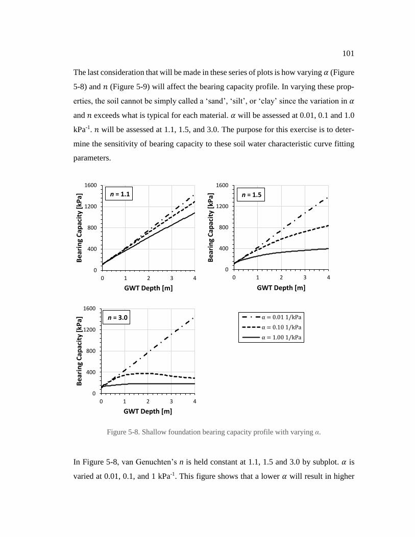
101
The last consideration that will be made in these series of plots is how varying 𝛼 (Figure
5-8) and 𝑛 (Figure 5-9) will affect the bearing capacity profile. In varying these prop-
erties, the soil cannot be simply called a ‘sand’, ‘silt’, or ‘clay’ since the variation in 𝛼
and 𝑛 exceeds what is typical for each material. 𝛼 will be assessed at 0.01, 0.1 and 1.0
kPa-1. 𝑛 will be assessed at 1.1, 1.5, and 3.0. The purpose for this exercise is to deter-
mine the sensitivity of bearing capacity to these soil water characteristic curve fitting
parameters.
Figure 5-8. Shallow foundation bearing capacity profile with varying α.
In Figure 5-8, van Genuchten’s n is held constant at 1.1, 1.5 and 3.0 by subplot. 𝛼 is
varied at 0.01, 0.1, and 1 kPa-1. This figure shows that a lower 𝛼 will result in higher
0
400
800
1200
1600
0 1 2 3 4
Be
arin
g C
apac
ity
[kP
a]
GWT Depth [m]
n = 1.1
0
400
800
1200
1600
0 1 2 3 4
Be
arin
g C
apac
ity
[kP
a]
GWT Depth [m]
n = 1.5
0
400
800
1200
1600
0 1 2 3 4
Bea
rin
g C
apac
ity
[kP
a]
GWT Depth [m]
n = 3.0
0500100015002000
-2 3
α = 0.01 1/kPa
α = 0.10 1/kPa
α = 1.00 1/kPa

102
bearing capacity. 𝛼 varies the shape of the soil water characteristic curve. Increasing 𝛼
decreases the air-entry suction, while decreasing 𝛼 increases the air-entry suction. For
lower 𝛼, air-entry occurs at a higher matric suction, which implies that the groundwater
table depth must be greater in order for air to begin rapidly entering the pores, and
thereby inducing suction stresses. For n = 3.0, bearing capacity profile shows a defini-
tive peak, and then begins to decrease for 𝛼 = 0.1 and 1.0 kPa-1. This is typical for
coarse-grained soils.
Figure 5-9. Shallow foundation bearing capacity profile with varying n. Note changing
ordinate across figures.
Figure 5-9 is similar to Figure 5-8 except that 𝛼 is held constant at 0.01 kPa−1,
0.1 kPa−1, and 1 kPa−1 for each subplot. For 𝛼 = 0.1 and 1 kPa-1, smaller values for
0
400
800
1200
1600
0 1 2 3 4
Be
arin
g C
apac
ity
[kP
a]
GWT Depth [m]
α = 0.01 kPa-1
0
400
800
1200
1600
0 1 2 3 4
Be
arin
g C
apac
ity
[kP
a]
GWT Depth [m]
α = 0.10 kPa-1
0
400
800
1200
1600
0 1 2 3 4
Bea
rin
g C
apac
ity
[kP
a]
GWT Depth [m]
α = 1.0 kPa-1
0500100015002000
-2 3
n = 1.1
n = 1.5
n = 3.0

103
n result in larger bearing capacity. For 𝛼 = 0.01 kPa-1, n = 1.1 and n = 3.0 have higher
bearing capacities than n = 1.5, although the difference is small. Again, this can also be
explained due to suction stresses. With n = 1.5, the average suction will be smaller
throughout the entire soil profile and at the depth of embedment (which is D = 0). Thus,
the average apparent cohesion cʹʹ and the effective stress at the depth of embedment
will be smaller, decreasing bearing capacity.
To summarize the findings in this section, Figure 5-8 and Figure 5-9, show that the van
Genuchten fitting parameters, 𝛼 and n, have the greatest influence on the behavior of
bearing capacity. An accurate determination of these parameters, and thus the soil water
characteristic curve, is thus crucial in calculating reasonable bearing capacity values. It
has been shown that other input parameters influence the bearing capacity of shallow
foundations in partially saturated soils, but these changes are small (or constant) as in
𝜃𝑠 and 𝜃𝑟, or only varying the unmodified portion of the bearing capacity equation, like
𝜙′. Flux 𝑞 also has a considerable influence on the bearing capacity, especially for clays
and silts.
5.3.2. Evaluation of van Genuchten’s 𝛼 and 𝑛
As mentioned, van Genuchten’s fitting parameters have the most significant influence
on bearing capacity performance for foundations in partially saturated soils. With that
in mind, these variables should be assessed more closely. The results presented in the
following figures will look more closely at these two parameters, varying them along
the x-axis (instead of zw) while holding the groundwater table depth fixed. The bearing
capacity will be calculated at depths of the groundwater table equal to 0 m, 1 m, 2 m,
3 m, 5 m, and 10 m while either varying 𝛼 or n. In this example, 𝜙′ = 30°, 𝜃𝑠 = 0.4,
𝜃𝑠 = 0.06, and 𝐷 = 0 m.
Figure 5-10 through Figure 5-12 plot bearing capacity with respect to van Genuchten’s
𝛼 fitting parameter while n is fixed at 1.1, 1.5, and 3.0. As mentioned, this is done at
various depths of groundwater tables.
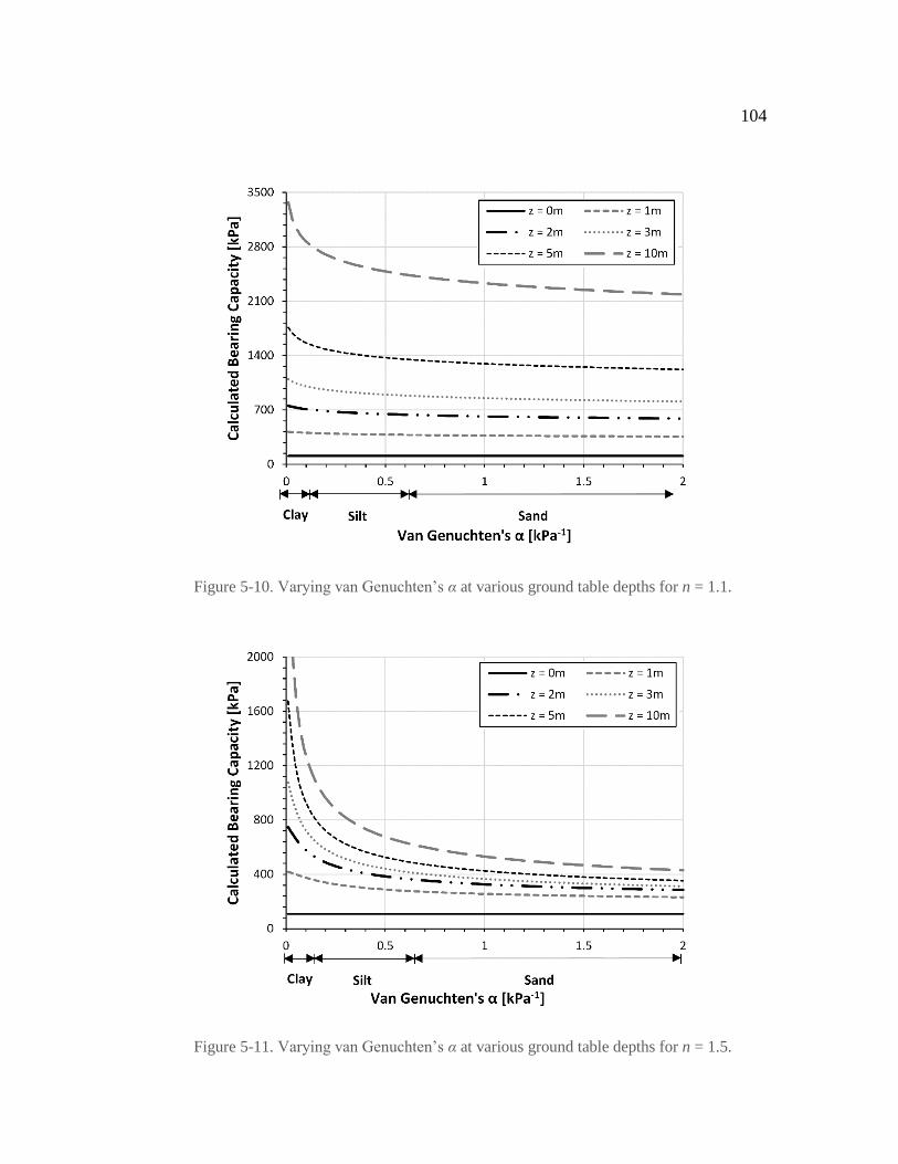
104
Figure 5-10. Varying van Genuchten’s α at various ground table depths for n = 1.1.
Figure 5-11. Varying van Genuchten’s α at various ground table depths for n = 1.5.

105
Figure 5-12. Varying van Genuchten’s α at various ground table depths for n = 3.0.
Figure 5-10 and Figure 5-11 exhibit different behavior than Figure 5-12. In these two
figures, as the depth of the groundwater table increases, the bearing capacity will al-
ways increase. This is the tendency of fine-grained soils (i.e., those with relatively low
n-values), where suction stress increases with matric suction. Figure 5-12 shows dif-
ferent behavior in that the groundwater table depth does not necessarily increase bear-
ing capacity. For a groundwater table at a depth of z = 2 m and higher 𝛼 values (typical
for silts and sands), the bearing capacity is greater than at any other groundwater table
depth. When 𝛼 decreases to values more typical of clays, the bearing capacity for z = 1
m is less than the other depths. This behavior is typical for coarse-grained soils, which
have limited suction stresses. In coarse-grained soils, the bearing capacity will initially
increase as the groundwater table depth increases due to suction stresses, but will then
decrease to the conventional Vesić solution as suction stress dissipates. Another notable
trend is that as n increases, the influence of 𝛼 on bearing capacity decreases for 𝛼 values
typical of silts and sands.

106
Figure 5-13. Varying van Genuchten’s n at various ground table depths for 𝛼 = 0.01 kPa-1.
Figure 5-14. Varying van Genuchten’s n at various ground table depths for 𝛼 = 0.1 kPa-1.

107
Figure 5-15. Varying van Genuchten’s n at various ground table depths for 𝛼 = 1 kPa-1.
Figure 5-13 to Figure 5-15 plot bearing capacity with respect to van Genuchten’s n
fitting parameter while 𝛼 is fixed at 0.01, 0.1, and 1 kPa-1. Figure 5-13 exhibits similar
behavior to Figure 5-10 and Figure 5-11, which shows that as the groundwater table
depth increases, bearing capacity also increases. This indicates that 𝛼 = 0.01 kPa−1
behaves predominately as a fine-grained soil. Figure 5-14 and Figure 5-15 behave the
same as Figure 5-12, where the bearing capacity does not necessarily increase with
groundwater table depth. These two figures show a transitory regime, labeled by sands,
where smaller groundwater table depths will have greater bearing capacities. Bearing
capacity decreases/drops significantly as n increases, especially for higher values of 𝛼.
The 5 m groundwater table in Figure 5-13 shows that the bearing capacity initially
decreases with increasing n, but then decreases. This indicates that the average apparent
cohesion across the failure surface does not necessarily decrease with an increase in n.
The results show that for low 𝛼, average suction stress may increase with n.

108
Figure 5-10 through Figure 5-15 have demonstrated the different behaviors of fine-
grained versus coarse-grained soils. In fine-grained soils (low 𝛼 and n), bearing capac-
ity is expected to increase with the groundwater table depth. This is due to the suction
stresses present in the soil, which will continue to increase with matric suction in fine-
grained soils. In coarse-grained soils (higher 𝛼 and n), bearing capacity does not nec-
essarily follow this pattern depending on the values of 𝛼 and n. As these values in-
crease, the influence of the suction decreases, and the calculated bearing capacity ap-
proaches the conventional solution, which is equal to the bearing capacity calculated in
dry conditions.
5.3.3. Other Considerations for Shallow Foundation Bearing Capacity
With these basic trends established, it is important to assess other factors concerning
shallow foundation bearing capacity. In this section the following will be addressed:
(1) a brief comparison between the modified approach and the conventional approach;
(2) discussion on phenomena where bearing capacity decreases and increases with foot-
ing width; and (3) the presentation of design charts for shallow foundations in partially
saturated soils.
Figure 5-16 show the bearing capacity profile for a theoretical sand (𝛼 = 1 kPa-1 and n
= 3) with an embedment depth D = 0 m. The bearing capacity profile is made for soils
with 𝜙′ = 25˚, 30˚, and 35˚. This figure actually shows that the conventional bearing
capacity equation performs well against the modified equation. There are portions
where the conventional approach will predict a bearing capacity greater than the mod-
ified approach. This is because the modified approach calculates a smaller average unit
weight, due to drainage in the pores, than the conventional method. Overall, there is
agreement between the two methods.

109
Figure 5-16. Comparison of the predicted bearing capacity for a sand using the modified and
conventional approach at various friction angles, D = 0 m.
Figure 5-17 plots the same bearing capacity profile, except that the foundation is em-
bedded at depth D = 1.5 m. As with the previous figure, the calculated bearing capacity
is the same between the conventional and modified equations for saturated (z = 0 m)
and dry conditions (the groundwater table is deep). For the modified approach, suction
will increase the effective stress at the depth of embedment 𝜎𝑧𝐷′ and also the average
apparent cohesion 𝑐′′. In the conventional approach, the soil weight is assumed to vary
linearly between D and D + B, which is why the conventional method does not predict
an increase in bearing capacity until z = D. The modified approach, however, indicates
that a shallow increase in bearing capacity should occur between z = 0 to D due to
suction. Apart from this exception, both solutions decently agree.
0
100
200
300
400
500
0 0.5 1 1.5 2 2.5 3
Cal
cula
ted
Bea
rin
g C
apac
ity
[kP
a]
Depth of GWT [m]
Modified Approach
Conventional Approach 𝜙′ = 35°
𝜙′ = 30°
𝜙′ = 25°

110
Figure 5-17. Comparison of the predicted bearing capacity for a sand using the modified and
conventional approach at various friction angles, D = 1.5 m.
Figure 5-18 and Figure 5-19 show how varying unsaturated properties affect the bear-
ing capacity profile. In these two example, the unsaturated soil parameters selected are
n = 3 and 𝛼 = 0.1 kPa-1. n was not decreased since as this soil would exhibit the fine-
grained behavior discussed in the previous section, Section 5.3.2, where ultimate bear-
ing capacity increases with groundwater table depth and does not return to the conven-
tional bearing capacity solution. Figure 5-18 and Figure 5-19 have embedment depths
of D = 0 and D = 1.5 m. In these two figures, a clear peak is achieved. This peak is
attributed to suction which is manifested in the effective vertical stress at the depth of
embedment 𝜎𝑧𝐷′ and apparent cohesion 𝑐′′. At higher depths, suction stresses will dis-
sipate due to smaller water contact area between particles.
0
500
1000
1500
2000
0 1 2 3 4
Cal
cula
ted
Bea
rin
g C
apac
ity
[kP
a]
Depth of GWT [m]
Modified Approach
Conventional Approach
𝜙′ = 35°
𝜙′ = 30°
𝜙′ = 25°

111
Figure 5-18. Comparison of the predicted bearing capacity between the modified and
conventional approach at various friction angles for a material with D = 0 m, n = 3, and α =
0.1 kPa-1.
Figure 5-19. Comparison of the predicted bearing capacity between the modified and
conventional approach at various friction angles for a material with D = 1.5 m, n = 3, and α =
0.1 kPa-1.
Figure 5-20 shows an interesting phenomena that was discussed in the Briaud and Gib-
bens (1997) analysis. Many load tests have shown that the bearing capacity does not
0
200
400
600
800
1000
0 1 2 3 4 5 6
Cal
cula
ted
Bea
rin
g C
apac
ity
[kP
a]
Depth of GWT [m]
Modified Approach
Conventional Approach
𝜙′ = 35°
𝜙′ = 30°
𝜙′ = 25°
0
500
1000
1500
2000
0 2 4 6 8 10
Cal
cula
ted
Be
arin
g C
apac
ity
[kP
a]
Depth of GWT [m]
Modified Approach
Conventional Approach
𝜙′ = 35°
𝜙′ = 30°
𝜙′ = 25°

112
always increase with footing with. The conventional bearing capacity equation does
not predict this phenomena since the footing width term in the equation, 0.5𝐵𝛾′, sug-
gests that increases in bearing capacity are linearly proportional to increases in footing
width. While this term is still used in the modified approach, variation in effective unit
weight 𝛾′, apparent cohesion 𝑐′′, and overburden 𝜎𝑧𝐷′ are dictated by the size and shape
of the failure surface. That being said, as the footing width increases, depth of the fail-
ure surface also increases. For this example, the groundwater table depth is 4 m. For
very small footing widths (B = 0.5 m), the failure surface will not extend below the
groundwater table and apparent cohesion 𝑐′′ and 𝛾′ will be greater. If the footing width
is large enough (B > 1.5 m), the failure surface will extend into the groundwater table,
decreasing average apparent cohesion and unit weight.
Figure 5-20. Comparison of the predicted bearing capacity for silt while varying the footing
width. This soil has zw = 4 m, 𝜙′ = 30˚ and D = 0.5 m.
As previously discussed, the unsaturated parameters 𝜃𝑟 and 𝜃𝑠 have little influence on
the behavior or performance of a shallow foundation (with the exception of clean sands)
but 𝛼 and n have been shown to contribute significantly to the calculated modified
bearing capacity. Figure 5-21 is a table of figures comparing the calculated bearing
0
250
500
750
1000
1250
1500
1750
0 1 2 3 4 5 6
Cal
cula
ted
Be
arin
g C
apac
ity
[kP
a]
Footing Width [m]
Modified Approach
Conventional Approach
113
capacity to five input parameters: friction angle 𝜙′, groundwater table depth 𝑧𝑤, footing
width 𝐵, van Genuchten’s 𝛼, and 𝑛. Cohesion c’, depth of embedment 𝐷, and specific
gravity 𝐺𝑠 have been shown to only incrementally affect bearing capacity for all values
of 𝜙′, 𝑧𝑤, 𝐵, 𝛼, and 𝑛. The consideration of c’, 𝐷, and 𝐺𝑠 would not produce interest-
ing results. In Figure 5-21 𝐺𝑠 = 2.65, 𝜃𝑠 = 0.4, 𝜃𝑟 = 0.06, and is considered to be a strip
footing.
In the development of Figure 5-21 it is important to note that a few variables can be
normalized: 𝑧𝑤 with 𝐵, 𝑞𝑢𝑙𝑡,𝑚𝑜𝑑𝑖𝑓𝑖𝑒𝑑 with 𝑞𝑢𝑙𝑡,𝑢𝑛𝑚𝑜𝑑𝑖𝑓𝑖𝑒𝑑, and 𝛼 with 𝑧𝑤. The depth of
the groundwater table and footing width can be normalized since the size and shape of
the failure surface will remain proportional. The modified bearing capacity and the un-
modified bearing capacity can be normalized by dividing the two since variation in
apparent cohesion, unit weight, and overburden will only increase (or decrease) accord-
ing the bearing, shape, and depth factors which are the same for the two equations. That
is, an increase in, say, apparent cohesion will always increase the bearing capacity by
a factor 𝑁𝑐𝜁𝑠𝑐𝜁𝑑𝑐 . Lastly, 𝛼𝜓 or 𝛼𝑧𝑤𝛾𝑤 will normalize the soil water characteristic
curve, as shown in Figure 5-22. In normalizing these variables, contours of
𝑞𝑢𝑙𝑡,𝑚𝑜𝑑𝑖𝑓𝑖𝑒𝑑/𝑞𝑢𝑙𝑡,𝑢𝑛𝑚𝑜𝑑𝑖𝑓𝑖𝑒𝑑 are plotted in Figure 5-21. These charts can be used in
design as a tool for predicting the bearing capacity of a shallow foundation in partially
saturated soils. If 𝐺𝑠, 𝜃𝑟, 𝜃𝑠, 𝑐′, or 𝐷 were to change, the bearing capacity would vary
by a fixed value, which can be calculated from the conventional bearing capacity equa-
tion.

114
𝜙′ = 40° 𝜙′ = 30° 𝜙′ = 20°
𝑧 𝑤/𝐵
=0
.5
𝑧 𝑤/𝐵
=1
𝑧 𝑤
/𝐵=
2
𝑧 𝑤/𝐵
=5
Figure 5-21. Table of figures for qmod/qunmod. The x and y axes of the table correspond to various ϕ' and zw/B ratios
respectively. For each individual figure, x and y axes are αzwγw and n, respectively.
van
Gen
uch
ten’s
𝑛
𝛼𝑧𝑤𝛾𝑤

115
Figure 5-22. Normailzation of the soil water characteristic curve.
Figure 5-21 summarizes the most prominent behavior shallow foundations in partially
saturated soils. Soils with low friction angle will have the tendency to be more influ-
enced by suction, which is indicated by contour lines with higher values. This does not
imply that calculated bearing capacities are higher. This figure also indicates that higher
values of 𝛼 and 𝑛 will calculate higher modified bearing capacities, especially as the
0.01 0.1 1 10 100 1 103
0
0.1
0.2
0.3
1/kPa
0.1/kPa
0.01/kPa
= z [kPa]
0.01 0.1 1 10 1000
0.1
0.2
0.3
1/kPa
0.1/kPa
0.01/kPa
= z

116
depth of the groundwater table increases. Regimes where the modified bearing capacity
is less than the unmodified bearing capacity exist where the contour is 1.0 or less. This
figure is fairly simple to use and implementation in practice would be easy when the
SWCC or soil type are known.
This section has covered other considerations for shallow foundation bearing capacity
in partially saturated soils. For sands, there is close agreement between the modified
approach and the conventional approach. Therefore, the use of the conventional bearing
capacity equation is suitable coarse-grained soils, but not fine-grained soils, where suc-
tion stresses are high. Footing width is an important consideration as this will control
the depth of the failure surface. Larger footings have larger failure surface, which may
be detrimental to the ultimate loading stress depending on the location of the failure
surface. Design charts for shallow foundations in partially saturated soils have been
introduced. For implementation of unsaturated soil in practice, ease and accessibility is
an important consideration, and design charts allow for quick estimates of the potential
increase (or decrease) in bearing capacity when compared to conventional method.
5.3.4. Vahedifard and Robinson (2015)
Vahedifard and Robinson (2015) built off of the work by Lu and Likos (2004), who
first developed a closed-form solution to the matric suction profile in soil with varying
rates of infiltration, and Vanapalli and Mohamed (2007), who have modified the Ter-
zaghi bearing capacity equation to account for partially saturated soils. Again, the
equation that was derived originally by Vanapalli and Mohamed (2007) is:
𝑞𝑢𝑙𝑡 = [𝑐′ + (𝑢𝑎 − 𝑢𝑤)𝑏(1 − 𝑆𝜓) tan 𝜙′ + (𝑢𝑎 −
𝑢𝑤)𝐴𝑉𝑅𝑆𝜓 tan 𝜙′] × 𝑁𝑐𝜉𝑐 + 0.5𝐵𝛾𝑁𝛾𝜉𝛾 5-2
The modified equation proposed by Vahedifard and Robinson (2015) is:

117
𝑞𝑢𝑙𝑡 = {𝑐′ + 𝑎(1 + 𝑆𝑒,AVR) tan 𝜙′ + [(𝑢𝑎 − 𝑢𝑤)𝑆𝑒]AVR tan 𝜙′}𝑁𝑐ξc
+ 𝑞0𝑁𝑞𝜉𝑞 + 0.5�̅�𝐵𝑁𝛾𝜉𝛾 5-3
Essentially the above equation was modified to account for three things: (1) inclusion
of a surcharge term denoted by 𝑞0; (2) modification to the cohesion term which is done
to include the apparent cohesion due to matric suction; and (3) averaged unit weight
values. The surcharge 𝑞0 is calculated as the effective stress, not including suction
stress, at the embedment depth 𝐷. Variation in soil unit weight �̅� and matric suction
(𝑢𝑎 − 𝑢𝑤) are calculated as the average across the stress bulb, 𝐷 to 𝐷 + 1.5𝐵. 𝑆𝑒,AVR
is the average saturation value across the stress bulb. 𝑎 is the air entry suction. Vahe-
difard and Robinson (2015) have segregated the effects of suction stress into two terms:
𝑎(1 + 𝑆𝑒,AVR) tan 𝜙′ and [(𝑢𝑎 − 𝑢𝑤)𝑆𝑒]AVR tan 𝜙′ where (𝑢𝑎 − 𝑢𝑤)𝑆𝑒 is suction
stress 𝜎𝑠. These two expressions account for suction up to the air-entry value and suc-
tions greater than the air-entry value respectively.
This approach is similar to the method used in this work with the following exceptions:
(1) no dry unit weight or saturated unit weight is assumed, this is controlled by the
variables 𝜃𝑟, 𝜃𝑠, and 𝐺𝑠; (2) the apparent cohesion due to suction stress is calculated
across the failure surface, as opposed to the average from D to D + B, and is not sepa-
rated into two different expressions; and (3) the surcharge 𝑞0 is inclusive to any suction
stress applied by unsaturated soils at the depth of embedment. Again, the apparent co-
hesion term used in this work is:
𝑐′′ = 𝜒𝜓 tan 𝜙′ 5-4
Which is integrated across the failure surface:
𝑐′′̅̅ ̅ =
∫ 𝑙 ∙ 𝑐′′𝑑𝑙
∫ 𝑙 𝑑𝑙 5-5

118
Equation 5-5 is directly implement into the conventional bearing capacity equation.
Since the approach provided by Vahedifard and Robinson (2015) is similar to the ap-
proach developed in this work, it is insightful to make comparisons between the two.
The following figures compare the parametric studies conducted by Vahedifard and
Robinson (2015) and a comparison made by the modified approach used in this thesis.
The comparison in Figure 5-23 and Figure 5-24 compares strip footings with a width
of 1 m over clay soil. The soil has the following properties:
Table 5-2. Input parameters for clay used in Vahedifard and Robinson (2015).
Properties
Value SWCC
Properties Values
𝝓′ 20 − 25° 𝛼 0.005 kPa−1 𝒄′ 10 kPa 𝑛 1.8 𝑮𝒔 2.65 𝜃𝑠 0.369
𝜃𝑟 0.0 𝑘𝑠 5 ∙ 10−8 m/s
Vahedifard and Robinson (2015) use an 18 kN/m3 soil for all groundwater table depths.
𝜃𝑠 was selected to fix the saturated unit weight to 20 kN/m3. The dry unit weight cor-
responding to this porosity is 16.4 kN/m3. This range brackets the value used by Vahe-
difard and Robinson (2015).

119
Figure 5-23. Calculated bearing capacity for hypothetical clay with D = 0 from Vahedifard
and Robinson (2015) compared to modified approach in this current work (left 𝜙′ = 25°,
right 𝜙′ = 20°).
Figure 5-24. Calculated bearing capacity for hypothetical clay with D = 1.5 m from
Vahedifard and Robinson 2015 compared to modified approach in this current work (left
𝜙′ = 25°, right 𝜙′ = 20°). Note changing ordinate across figures.
0
1000
2000
3000
4000
0 3 6 9 12
Cal
cula
ted
Bea
rin
g C
apac
ity
[kP
a]
Depth of GWT [m]
q = 1.15E-8 m/s
q = 0 m/s
q = -3.14E-8 m/s
V & H (2015)
0
1000
2000
3000
4000
0 3 6 9 12
Cal
cula
ted
Be
arin
g C
apac
ity
[kP
a]
Depth of GWT [m]
q = 1.15E-8 m/s
q = 0 m/s
q = -3.14E-8 m/s
V & R (2015)
0
1000
2000
3000
4000
5000
0 3 6 9 12
Cal
cula
ted
Be
arin
g C
apac
ity
[kP
a]
Depth of GWT [m]
q = 1.15E-8 m/sq = 0 m/sq = -3.14E-8 m/sV & R (2015)
0
1000
2000
3000
0 3 6 9 12
Cal
cula
ted
Be
arin
g C
apac
ity
[kP
a]
Depth of GWT [m]
q = 1.15E-8 m/sq = 0 m/sq = -3.14E-8 m/sV & R (2015)
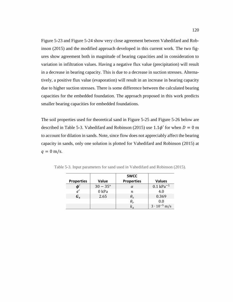
120
Figure 5-23 and Figure 5-24 show very close agreement between Vahedifard and Rob-
inson (2015) and the modified approach developed in this current work. The two fig-
ures show agreement both in magnitude of bearing capacities and in consideration to
variation in infiltration values. Having a negative flux value (precipitation) will result
in a decrease in bearing capacity. This is due to a decrease in suction stresses. Alterna-
tively, a positive flux value (evaporation) will result in an increase in bearing capacity
due to higher suction stresses. There is some difference between the calculated bearing
capacities for the embedded foundation. The approach proposed in this work predicts
smaller bearing capacities for embedded foundations.
The soil properties used for theoretical sand in Figure 5-25 and Figure 5-26 below are
described in Table 5-3. Vahedifard and Robinson (2015) use 1.1𝜙′ for when 𝐷 = 0 m
to account for dilation in sands. Note, since flow does not appreciably affect the bearing
capacity in sands, only one solution is plotted for Vahedifard and Robinson (2015) at
𝑞 = 0 m/s.
Table 5-3. Input parameters for sand used in Vahedifard and Robinson (2015).
Properties
Value SWCC
Properties Values
𝝓′ 30 − 35° 𝛼 0.1 kPa−1 𝒄′ 0 kPa 𝑛 4.0 𝑮𝒔 2.65 𝜃𝑠 0.369
𝜃𝑟 0.0 𝑘𝑠 3 ∙ 10−5 m/s

121
Figure 5-25. Calculated bearing capacity for hypothetical sand with D = 0 m from Vahedifard
and Robinson 2015 compared to modified approach in this current work.
Figure 5-26. Calculated bearing capacity for hypothetical sand with D = 1.5 m from
Vahedifard and Robinson (2015) compared to modified approach in this current work.
Figure 5-25 and Figure 5-26 show that the approach proposed in this work and by
Vahedifard and Robinson (2015) do not have good agreement in calculated bearing
capacities in sands. These two figures, however, show agreement in that sandy soils are
0
1000
2000
3000
0 3 6 9 12
Cal
cula
ted
Bea
rin
g C
apac
ity
[kP
a]
Depth of GWT [m]
q = 1.15E-8 m/s
q = 0 m/s
q = -3.14E-8 m/s
V & R (2015)
𝜙′ = 35° × 1.1
𝜙′ = 35° × 1.1
𝜙′ = 30° × 1.1
𝜙′ = 30° × 1.1
0
2000
4000
6000
0 3 6 9 12
Cal
cula
ted
Be
arin
g C
apac
ity
[kP
a]
Depth of GWT [m]
q = 1.15E-8 m/s
q = 0 m/s
q = -3.14E-8 m/s
V & H (2015)
𝜙′ = 35°
𝜙′ = 30°
𝜙′ = 35°
𝜙′ = 30°

122
largely unaffected by variation in flux. There is no noticeable difference between infil-
tration, evaporation, and no flow. To assess the difference more closely, solutions to
bearing capacity for the current proposed method, the Vesić approach, and Vahedifard
and Robinson (2015) are compared in Figure 5-27 and Figure 5-28. For the Vesić so-
lution, the assumed moist unit weight is 𝛾 = 18 kN/m3, which does not fluctuate as
the groundwater table moves. In Figure 5-27, solutions for the surface foundation with
1.1𝜙′ are presented. In Figure 5-28, solutions for the embedded foundation are pre-
sented. Only solutions for 𝑞 = 0 m/s are presented in these figures.
Figure 5-27. Comparison of calculated bearing capacity profiles using the proposed approach,
the Vesić solution, and Vahedifard and Robinson (2015) for a surface foundation (left: 𝜙′ =35° × 1.1, right: 𝜙′ = 30° × 1.1).
0
1000
2000
3000
0 3 6 9 12
Cal
cula
ted
Be
arin
g C
apac
ity
[kP
a]
Depth of GWT [m]
This Work
Vesic Approach
V & R (2015)
0
300
600
900
1200
0 3 6 9 12
Cal
cula
ted
Be
arin
g C
apac
ity
[kP
a]
Depth of GWT [m]
This Work
Vesic Approach
V & R (2015)

123
Figure 5-28. Comparison of calculated bearing capacity profiles using the proposed approach,
the Vesić solution, and Vahedifard and Robinson (2015) for an embedded foundation (left:
𝜙′ = 35°, right: 𝜙′ = 30°).
Figure 5-27 and Figure 5-28 show that the approach proposed in this work generally
has good agreement with the Vesić solution. Vahedifard and Robinson (2015) calcu-
lated around twice the amount predicted by the Vesić equation for each scenario. Since
sands are being modeled, the bearing capacity solutions should be similar when zw = 0
m and when zw is deep. This is the case for the approach proposed in this work. There
are some discrepancies between the current proposed solution and the Vesić solution
for the embedded foundation at deep groundwater tables. This is attributed to a differ-
ence in definition for soil unit weight. The unit weight in the proposed approach is
allowed to vary between 20 kN/m3 and 16.4 kN/m3, while 18 kN/m3 is fixed for the
Vesić solution. The air-entry suction for sands has the tendency to be relatively low,
therefore, the predicted unit will quickly tend towards 16.4 kN/m3 as the groundwater
table increases in depth. Differences between the approach proposed by Vahedifard and
Robinson (2015) and in this work can be attributed to either different bearing capacities
(although the differences should not be this large) or human error.
0
1000
2000
3000
4000
5000
0 3 6 9 12
Cal
cula
ted
Bea
rin
g C
apac
ity
[kP
a]
Depth of GWT [m]
This Work
Vesic Approach
V & H (2015)
0
500
1000
1500
2000
2500
0 3 6 9 12
Cal
cula
ted
Bea
rin
g C
apac
ity
[kP
a]
Depth of GWT [m]
This WorkVesic ApproachV & R (2015)

124
5.4. Parametric Study on the Modified 𝛽-method
5.4.1. Development of Side Resistance Profiles
In this section sensitivity of the modified beta method will be assessed with various
soil properties. This study will use the same soils described at the beginning of this
chapter in Section 5.2, theoretical sand, silt, and clay. For each of these soil types, the
frictional resistance will be calculated as a function of groundwater table depth. A plot
comparing the groundwater table depth to total unit side resistance 𝑞𝑠 will subsequently
referred to as the side resistance profile. The total unit side resistance is defined by Eq.
5-6.
𝑞𝑠 = ∫ 𝑓𝑠
𝐷
0
𝑑𝑧 → 𝐹𝑜𝑟𝑐𝑒/𝑃𝑒𝑟𝑖𝑚𝑒𝑡𝑒𝑟 5-6
where 𝑓𝑠 is the side resistance of the pile or drilled shaft, and 𝐷 is the pile depth. 𝑓𝑠 is
measured in units of pressure (kPa) and describes the frictional resistance at a single
point along the deep foundation. Integrating by depth yields 𝑞𝑠 which has units of kN/m
or MN/m. To calculate the total side resistance 𝑄𝑠, the total unit side resistance can be
multiplied by the circumference of the pile or drilled shaft for units of kN or MN. The
shape of the pile or drilled shaft is not important in this discussion, therefore, there is
no selection of pile diameter. Eq. 5-7 describes the side resistance above the ground-
water table, which was developed in Section 3.3.1.
𝑓𝑠 = (𝐾0 tan 𝛿 +
𝜎𝑠
𝜎𝑣tan 𝛿 +
𝑐′
𝜎𝑣) 𝜎𝑣 = 𝛽′𝜎𝑣 5-7
where all variables are as previously described. In this formulation of the 𝛽′-method,
matric suction is considered in two ways: (1) variation of the at-rest earth pressure co-
efficient; and (2) variation in suction stress. Equations for suction stress 𝜎𝑠, at-rest earth
pressure coefficient 𝐾0, and vertical effective stress 𝜎𝑣 are discussed in Section 3.3.
Figure 5-29 plots the suction stress profile for the theoretical sand, silt, and clay.

125
Figure 5-29. Suction stress profile above the groundwater table for theoretical sand, silt, and
clay (θs = 0.4, θr = 0.06, q = 0 m/s for each figure). Note changing abscissa across figures.
These suction stress profiles will serve as the basis for comparing the difference in
performance of sand, silt, and clay in partially saturated soils. As a general note, suction
stresses for sands are significantly smaller than silts and clays, and also peak shortly
above the groundwater table. Clays have the largest suction stresses. Using the suction
stress profile, 𝐾0 (Section 3.3.1) can be calculated as a function of depth from the sur-
face. This requires an assumption for the groundwater table depth. Finally, with these
considerations side resistance 𝑓𝑠 can be calculated according to the modified 𝛽-method
in Eq. 5-7. Figure 5-30 plot the vertical effective stress profile as a function of depth
from the soil surface for groundwater table depths of 0 m, 5 m, 10 m, 20 m, and 30 m.
The vertical effective stress is calculated from van Genuchten (1980) SWCC and is
discussed in Section 3.3.3. In this figure the specific gravity is 2.65.
0
1
2
3
4
5
0 0.25 0.5 0.75
Dis
tan
ce A
bo
ve G
WT
[m]
σs [kPa]
San
d, n
= 3
.0α
= 1
1/k
Pa
0
5
10
15
20
25
30
0 25 50 75
σs [kPa]Si
lt,n
= 1
.5α
= 0
.1 1
/kP
a
0
5
10
15
20
25
30
0 100 200 300
σs [kPa]
Cla
y, n
= 1
.1α
= 0
.01
1/k
Pa

126
Figure 5-30. Vertical effective stress as a function of depth from soil surface for theoretical
sand, silt, and clay (θs = 0.4, θr = 0.06, q = 0 m/s, Gs = 2.65 for each figure).
The only significant trend in this figure is that clay and silts with the same porosity and
specific gravity will generally have greater vertical stress than a similar sand. This in-
dicates that silts and clays retain a greater volume of water in pores than do sands,
increasing the soil unit weight. Once the soil profile and suction stresses are known,
the modified beta, 𝛽′, can be calculated. Figure 5-31 plot the modified beta as a function
of depth from the soil surface for groundwater table depths of 0 m, 5 m, 10 m, 20 m,
and 30 m. In this figure Poisson’s ratio 𝜈 and the interface friction angle 𝛿 are 0.3 and
30° respectively.
0
5
10
15
20
25
30
0 250 500 750
De
pth
fro
m S
urf
ace
[m]
0
5
10
15
20
25
30
0 250 500 750
σ' [kPa]
0
5
10
15
20
25
30
0 250 500 750
0
00.20.40.6GWT = 0 m GWT = 5 m GWT = 10 m GWT = 20 m GWT = 30 m
San
d, n
= 3
.0
α =
1 1
/kP
a
Silt
, n =
1.5
α
= 0
.1 1
/kP
a
Cla
y, n
= 1
.1
α =
0.0
1 1
/kP
a

127
Figure 5-31. Modified β’ as a function of depth from soil surface for theoretical sand, silt, and
clay (θs = 0.4, θr = 0.06, q = 0 m/s, Gs = 2.65, ν = 0.3, δ = 30˚ for each figure).
Figure 5-31 shows the most important trends in the understanding of deep foundations
in partially saturated soils. First, sands predict little influence from partially saturated
soils; there is little to no deviation from the conventional 𝛽, which is calculated as
𝜈 tan 𝛿 /(1 − 𝜈) = 0.24. This is also the same value that would be predicted for silts
and clays if the conventional approach was used and δ = 30˚ and ν = 0.3. Silts and
clays, however, have a different trend, especially near the surface. When 𝛽′ is equal to
zero, tension cracking is predicted near and no shear strength between the soil and pile
is achieved. Clays will typically have deeper tension cracks than silts. At depths below
tension cracking, silts and clays are highly influenced by suction stress, which is indi-
cated by the 𝛽′ values that are greater than 0.24. Once this 𝛽′ profile is known, side
resistance can be calculated. Figure 5-32 plot the side resistance as a function of depth
from the soil surface for groundwater table depths of 0 m, 5 m, 10 m, 20 m, and 30 m.
In this figure Poisson’s ratio 𝜈 and the interface friction angle 𝛿 are 0.3 and 30° respec-
tively.
0
5
10
15
20
25
30
0 0.2 0.4 0.6
De
pth
fro
m S
urf
ace
[m]
0
5
10
15
20
25
30
0 0.2 0.4 0.6
β'
0
5
10
15
20
25
30
0 0.2 0.4 0.6
0
00.20.40.6GWT = 0 m GWT = 5 m GWT = 10 m GWT = 20 m GWT = 30 m
San
d, n
= 3
.0
α =
1 1
/kP
a
Silt
, n =
1.5
α
= 0
.1 1
/kP
a
Cla
y, n
= 1
.1
α =
0.0
1 1
/kP
a

128
Figure 5-32. Side resistance as a function of depth from soil surface for theoretical sand, silt,
and clay (θs = 0.4, θr = 0.06, q = 0 m/s for each figure).
Figure 5-32 show the general trends in the behavior of theoretical sand, silt, and clay.
Silts and clays achieve cracking (when fs = 0) as the groundwater table increases in
depth. Tension cracking is not observed in sands since suction stress are low. Although
suction stresses cause cracking in silts and clays, it also results in large increases for
side resistance. For all three soil types, side resistance increases with depth due to an
increase in the vertical stress with depth. This vertical effective stress causes 𝑓𝑠 to in-
crease seemingly linearly with depth since the large majority of strength comes from
the vertical stress term (𝛽𝜎𝑣), however, suction stresses are present (especially in silts
and clays) through the expression 𝜎𝑠 tan 𝛿 that causes non-linearity in these plots. In-
tegrating any line in Figure 5-32 from 0 to the pile length L calculates a single value of
𝑞𝑠 for a specific groundwater table depth. If this same integral is conducted for many
groundwater table depths, 𝑞𝑠 can be plotted as a function of 𝑧𝑤, which is subsequently
called the side resistance profile.
0
5
10
15
20
25
30
0 100 200
De
pth
fro
m S
urf
ace
[m]
0
5
10
15
20
25
30
0 100 200
fs = βσv + σstanδ [kPa]
0
5
10
15
20
25
30
0 100 200
0
00.20.40.6GWT = 0 m GWT = 5 m GWT = 10 m GWT = 20 m GWT = 30 m
San
d, n
= 3
.0
α =
1 1
/kP
a
Silt
, n =
1.5
α
= 0
.1 1
/kP
a
Cla
y, n
= 1
.1
α =
0.0
1 1
/kP
a

129
For this parametric study, the side resistance profile will be considered for deep foun-
dation with lengths of 10 m, 15 m, 20 m, 25 m, and 30 m and groundwater table depths
ranging from 0 m to 30 m. The influence of Poisson’s ratio ν on the modified 𝛽-method
in partially saturated soils will be assessed by varying ν at 0.2, 0.3, and 0.4. It is im-
portant to note that interface friction angle 𝛿 will not be varied since this expression
has not been modified. 𝛿 will be taken as 30° for the remainder of this section. Values
for 𝑞𝑠 can be adjusted to a different interface friction angle by multiplying 𝑞𝑠 by
tan 𝛿 / tan 30°. As mentioned previously, the three soil types being considered are the
theoretical sand, silt, and clay. Table 5-4 summarizes the three soil types and
Table 5-4. Soil properties used in this parametric study
Property 𝜶 (𝐤𝐏𝐚−𝟏) 𝒏 𝒌𝒔 (𝐦/𝐬) 𝜽𝒔 𝜽𝒓
Clay 0.01 1.1 10-7 0.4 0.06
Silt 0.10 1.5 10-6 0.4 0.06
Sand 1.00 3.0 10-5 0.4 0.06
5.4.2. Evaluation of Side Resistance Profiles
Figure 5-33 presents the side resistance profile for theoretical sand, silt, and clay. This
profile was calculated according to Eq. 5-7 and is the integral of the three plots in
Figure 5-32 from 0 m to the length of the pile L. In this figure 𝜈 = 0.3, 𝐺𝑠 = 2.65, 𝜃𝑟 =
0.06, and 𝜃𝑠 = 0.4. As mentioned, the groundwater table depth varies from 0 m to 30
m. Pile lengths are assessed at 10 m, 15 m, 20 m, 25 m, and 30 m.

130
Figure 5-33. Side resistance profiles for theoretical sand, silt and clay (𝜈 = 0.3, 𝐺𝑠 = 2.65, 𝜃𝑟
= 0.06, and 𝜃𝑠 = 0.4) (unit side resistance given in force/unit perimeter)
Figure 5-33 shows several interesting trends between the three different soil types. The
first thing to note is that for each pile length, unit side resistance will generally either
increase to an asymptotic limit or achieve a peak resistance and begin to decrease (as
shown in the clay for L = 10 m). Generally, as the depth of the groundwater table in-
creases side resistance increases as well. This is mostly due to the increase in vertical
effective stress as porewater pressures dissipate. Clays and silts have higher peak unit
side resistance than do sands, which is attributed to the high suction stresses in these
soils. The last notable trend is that when the groundwater table extends below 10 m for
the 10 m pile embedded in clay, effects of tension cracking begin to manifest in a de-
creased side resistance. Eventually, side resistance is zero when the groundwater table
is 25 m. This implies that the tension cracks extend to a depth of 10 m.
San
d, n
= 3
.0
α =
1 1
/kP
a
Silt
, n =
1.5
α
= 0
.1 1
/kP
a
Cla
y, n
= 1
.1
α =
0.0
1 1
/kP
a

131
Figure 5-34 through Figure 5-36 study the effects volume/mass properties on theoreti-
cal silt. Silt was selected for these comparisons as silts typically have an intermediate
soil water characteristic curve relative to sands and clays. This will serve to generalize
the effects of varying specific gravity, porosity, and residual water content. In these
figures, all other variables are held constant, so that effects from 𝜃𝑟, 𝜃𝑠, or 𝐺𝑠 can be
individually characterized. Figure 5-34 sets the specific gravity at 2.60, 2.65, and 2.70
from left to right.
Figure 5-34. Side resistance profiles for theoretical silt with varying specific gravity (𝑛 = 1.5,
𝛼 = 0.1 kPa-1, 𝜈 = 0.3, 𝜃𝑟 = 0.06, and 𝜃𝑠 = 0.4) (unit side resistance given in force/unit perim-
eter)
Other than increasing the unit weight of the soil (and thus 𝜎𝑣), varying specific gravity
does not significantly change the behavior of the side resistance curves. It can be con-
cluded that the specific gravity has little influence on the mean modified 𝛽 profile.
Figure 5-35 sets 𝜃𝑟 equal to 0.02, 0.04, and 0.06 from left to right. Figure 5-36 sets 𝜃𝑠
equal to 0.35, 0.40, and 0.45 from left to right.

132
Figure 5-35. Side resistance profiles for theoretical silt with varying residual water content (𝑛
= 1.5, 𝛼 = 0.1 kPa-1, 𝜈 = 0.3, 𝐺𝑠 = 2.65, and 𝜃𝑠 = 0.4) (unit side resistance given in force/unit
perimeter)
San
d, n
= 3
.0
α =
1 1
/kP
a
Silt
, n =
1.5
α
= 0
.1 1
/kP
a
Cla
y, n
= 1
.1
α =
0.0
1 1
/kP
a

133
Figure 5-36. Side resistance profiles for theoretical silt with varying saturated water content
(𝑛 = 1.5, 𝛼 = 0.1 kPa-1, 𝜈 = 0.3, 𝐺𝑠 = 2.65, and 𝜃𝑟 = 0.06) (unit side resistance given in
force/unit perimeter)
These two figures shows that varying the saturated and residual water contents over a
reasonable range of values does not significantly change the performance or behavior
of a deep foundation. Increasing the residual water content will cause more water to be
retained in soil pores at high suctions, which will slightly increase the side resistance.
Decreasing the porosity increases the unit weight of the soil, which will also increase
side resistance. It is concluded that properties pertaining to soil volume and mass (𝜃𝑟,
𝜃𝑠, and 𝐺𝑠) do appreciably affect the predicted 𝑞𝑠.
Another consideration that can be made is the influence of varying water flow rates to
account for infiltration and evaporation. Fluctuation in flow will be studied for both
clay and silts (sands will not be included since suction stresses are low and negligible)
which have an assumed permeability of 𝑘𝑠 = 10−7 m/s and 𝑘𝑠 = 10−6 m/s respec-
tively. Figure 5-37 plot different 𝜎𝑠 for clays using a flow rate of 𝑞 = 0.2𝑘𝑠 (evapora-
tion), 𝑞 = 0 m/s, and 𝑞 = −0.2𝑘𝑠 (infiltration).
San
d, n
= 3
.0
α =
1 1
/kP
a
Silt
, n =
1.5
α
= 0
.1 1
/kP
a
Cla
y, n
= 1
.1
α =
0.0
1 1
/kP
a

134
Figure 5-37. Suction stress profiles of theoretical clay for flowrates of q = -0.2ks, 0, and 0.2ks.
The suction stress profile shows that positive flux (evaporation) will increase the suc-
tion stress. In this example, suction is thermodynamically limited to 106 kPa. Negative
flux (infiltration) will decrease the suction stress.
Figure 5-38 calculates the side resistance profile for theoretical clay exposed to
flowrates of q = -0.2ks (infiltration), 0, and 0.2ks (evaporation). During evaporation,
side resistance will decrease when compared to q = 0. During infiltration, the matric
suction throughout the profile is decreased, but this will also decrease the depth of ten-
sion cracking which increases the length along the pile where frictional resistance can
develop. This leads to an increased side resistance for clays exposed to infiltration.
0
5
10
15
20
25
30
0 100 200 300 400
Dis
tan
ce A
bo
ve G
WT
[m]
0
5
10
15
20
25
30
0 100 200 300 400
σs [kPa]
0
5
10
15
20
25
30
0 100 200 300 400
Cla
y q
= -
0.2
k s
Cla
y q
= 0
Cla
y q
= 0
.2k s

135
Figure 5-38. Side resistance profiles of theoretical clay for flowrates of q = -0.2ks, 0, and 0.2ks
(𝑛 = 1.5, 𝛼 = 0.1 kPa-1, 𝜈 = 0.3, 𝐺𝑠 = 2.65, and 𝜃𝑟 = 0.06) (unit side resistance given in
force/unit perimeter)
The same example is done for silt which has 𝑘𝑠 = 10−6 m/s. Figure 5-39 plots 𝜎𝑠 for
the theoretical silt exposed to flowrates of q = -0.2ks (infiltration), 0, and 0.2ks (evapo-
ration). Note that this figure is plotted as distance above the groundwater table so that
it is applicable to all groundwater table locations.
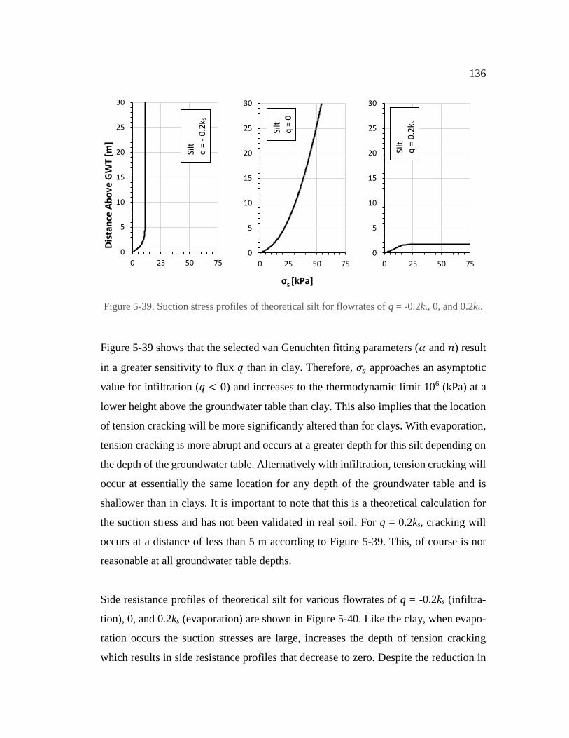
136
Figure 5-39. Suction stress profiles of theoretical silt for flowrates of q = -0.2ks, 0, and 0.2ks.
Figure 5-39 shows that the selected van Genuchten fitting parameters (𝛼 and 𝑛) result
in a greater sensitivity to flux 𝑞 than in clay. Therefore, 𝜎𝑠 approaches an asymptotic
value for infiltration (𝑞 < 0) and increases to the thermodynamic limit 106 (kPa) at a
lower height above the groundwater table than clay. This also implies that the location
of tension cracking will be more significantly altered than for clays. With evaporation,
tension cracking is more abrupt and occurs at a greater depth for this silt depending on
the depth of the groundwater table. Alternatively with infiltration, tension cracking will
occur at essentially the same location for any depth of the groundwater table and is
shallower than in clays. It is important to note that this is a theoretical calculation for
the suction stress and has not been validated in real soil. For q = 0.2ks, cracking will
occurs at a distance of less than 5 m according to Figure 5-39. This, of course is not
reasonable at all groundwater table depths.
Side resistance profiles of theoretical silt for various flowrates of q = -0.2ks (infiltra-
tion), 0, and 0.2ks (evaporation) are shown in Figure 5-40. Like the clay, when evapo-
ration occurs the suction stresses are large, increases the depth of tension cracking
which results in side resistance profiles that decrease to zero. Despite the reduction in
0
5
10
15
20
25
30
0 25 50 75
Dis
tan
ce A
bo
ve G
WT
[m]
0
5
10
15
20
25
30
0 25 50 75
σs [kPa]
0
5
10
15
20
25
30
0 25 50 75
Silt
q
= -
0.2
k s
Silt
q
= 0
Silt
q
= 0
.2k s

137
suction stress, infiltration produces greater side resistance than when q = 0 m/s. This is
attributed to the reduction in tension cracking.
Figure 5-40. Side resistance profiles of theoretical silt for flowrates of q = -0.2ks, 0, and 0.2ks
(𝑛 = 1.5, 𝛼 = 0.1 kPa-1, 𝜈 = 0.3, 𝐺𝑠 = 2.65, and 𝜃𝑟 = 0.06) (unit side resistance given in
force/unit perimeter)
As mentioned in the shallow foundation parametric study, 𝛼 and 𝑛 are the most im-
portant variables in determine the influence of suction stress on foundation perfor-
mance. Figure 5-41 through Figure 5-43 plot the side resistance profiles for various
values of 𝛼 (0.01 kPa-1, 0.1 kPa-1, and 1 kPa-1) and n (1.1, 1.5, and 3.0). Figure 5-41,
Figure 5-42, and Figure 5-43 have a fixed Poisson’s ratio of 0.2, 0.3, and 0.4 respec-
tively. These figures were intended to show the extent in variation between values of
total unit side resistance calculated in this work while varying unsaturated soil proper-
ties. Since 𝜃𝑟, 𝜃𝑠, and 𝐺𝑠 do not vary the results significantly, these charts can be used
in a design scenario for the selection of unit side resistance for normally consolidated
soils, especially when the soil water characteristic curve is known. In all three figures,
𝜃𝑟 = 0.06, 𝜃𝑠 = 0.40, and 𝐺𝑠 = 2.65.

138
Figure 5-41. Side resistance profiles for 𝜈 = 0.2 at various 𝑛 and 𝛼 values.

139
Figure 5-42. Side resistance profiles for 𝜈 = 0.3 at various 𝑛 and 𝛼 values.
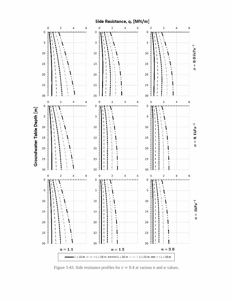
140
Figure 5-43. Side resistance profiles for 𝜈 = 0.4 at various 𝑛 and 𝛼 values.

141
Figure 5-41 through Figure 5-43 summarizes the results of the parametric study for the
side resistance of deep foundations in normally-consolidated soils. First, as the Pois-
son’s ratio increases, the influence of tension cracking decreases. Soils with large ν are
will generally have a greater horizontal strain, and thus be prone to less cracking. Con-
sequently, a smaller Poisson’s ratio will cause smaller horizontal strain and thus hori-
zontal stress in soils, which then reduces the required suction to produce tension crack-
ing. The subplot in Figure 5-41 exhibits interesting behavior for 𝛼 = 0.01 kPa-1 and n
= 3.0. In this figure, total unit side resistance initially decreases as the groundwater
table depth increases, but then begins to increase again. This can be explained through
the K0 profile, which is calculated for five different groundwater depths (0 m, 5 m, 10
m, 20 m, and 30 m) in Figure 5-44.
Figure 5-44. K0 as a function of depth from soil surface for α = 0.01 kPa-1, and n = 3.0 for
fixed groundwater table depths (θs = 0.4, θr = 0.06, q = 0 m/s, Gs = 2.65, ν = 0.2, δ = 30˚)
Figure 5-44 indicates that for a soil with 𝛼 = 0.01 kPa-1 and 𝑛 = 3.0, as the groundwater
table depth increases, the depth of cracking (which occurs when K0 = 0) initially in-
creases, but then decreases at zw = 30 m. What this implies is that when the groundwater
0
5
10
15
20
25
30
0 0.2 0.4 0.6
D [
m]
K0
0
00.20.40.6GWT = 0 m GWT = 5 m GWT = 10 m GWT = 20 m GWT = 30 m

142
table is deep (30 m), the suction stress is sufficiently small and the vertical stress is
sufficiently large enough to limit cracking.
Figure 5-41 through Figure 5-43 generally show that the depth of tension cracking will
increase for smaller Poisson’s ratios. This also implies that the length along which side
resistance can develop is shorter. Across all Poisson’s ratios, the matric suction and
suction stress profile remains the same. Therefore, soils with a higher Poisson’s ratio
will be influenced less by tension cracking. That is why the side resistance profiles for
ν = 0.4 do not decrease to zero. On the other hand, for ν = 0.2, the side resistance often
decreases with groundwater table depth due to tension cracks.
Another trend from Figure 5-41 through Figure 5-43 is the distinction between fine and
coarse grained material. Generally, for large 𝛼 and 𝑛 values (i.e. sands) the soil will
behave similar to the soil will be largely uninfluenced by matric suction. The depth of
tension cracking is also smaller (or non-existent) for larger values of 𝛼 and 𝑛. Tension
cracks are generally larger for smaller 𝛼 and 𝑛 (i.e. clays) values. In general, larger
Poisson’s ratios produces a greater transfer in vertical to horizontal stresses, resulting
stronger soils that are less influenced by tension cracking. Soils with larger Poisson’s
ratios will also have larger side resistance due to suction stresses. Since less cracking
occurs, there is more pile length to accumulate resistance due to suction and vertical
stresses.
In this last example, the modified 𝛽-method will be compared to the conventional ap-
proach. In the conventional approach, variation in K0 due to suction stress will be ne-
glected. That is K0 will be fixed to 𝜈/(1 − 𝜈), which for 𝜈 = 0.2, 0.3, and 0.4 is 0.25,
0.429, and 0.667. The conventional 𝛽-method also ignored additional strength from
suction stress, which is manifested in the expression 𝜎𝑠 tan 𝛿 = 𝜒𝜓 tan 𝛿. For this ex-
ample, the same 𝛾 profile will be used for both the conventional and modified ap-
proaches. The 𝛾 is based off of the van Genuchten (1980) SWCC, but it is assumed that
from exploratory drilling, similar unit weight values could be discovered. The unit

143
weight profile is plotted as a function of distance above the groundwater table, where
0 is at the groundwater table. This is presented in Figure 5-45.
Figure 5-45. Unit weight profile for theoretical clay (θs = 0.4, θr = 0.06, q = 0 m/s, Gs = 2.65,
α = 0.01 kPa-1, n = 1.1)
In Figure 5-45, the unit weight profile is plotted for theoretical clay. Clay was selected
because of its sensitivity to matric suction, resulting in larger suction stresses and po-
tentially more tension cracking. At the groundwater table, the pores are fully saturated
and the unit weight is equal to 19.5 kN/m3, which is calculated from 𝛾𝑤(𝐺𝑠(1 − 𝜃𝑠) +
𝜃𝑠). As the distance above the groundwater table increases, the unit weight will de-
crease to an asymptotic value of 16.2 kN/m3, which is calculated from
𝛾𝑤(𝐺𝑠(1 − 𝜃𝑠) + 𝜃𝑠). Below the groundwater table, the soil unit weight is calculated
as the buoyant unit weight, which in this case is 9.7 kN/m3. Using this soil profile, the
side resistance profile can be calculated for theoretical sands for both the modified and
conventional approach. This profile is calculated for 𝜈 = 0.2, 0.3, and 0.4, which is
presented in Figure 5-46.
0
5
10
15
20
25
30
15 16 17 18 19 20
Dis
tan
ce A
bo
ve G
WT
[m]
Unit Weight γ, [kN/m3]
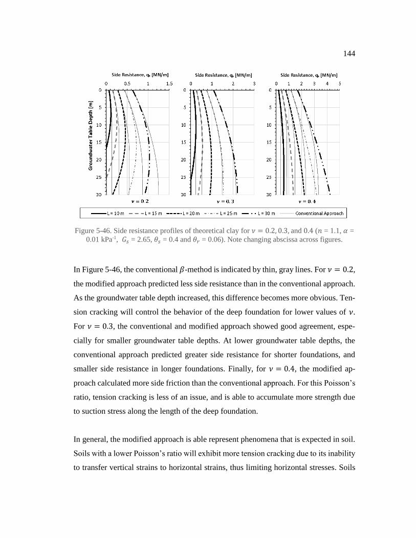
144
Figure 5-46. Side resistance profiles of theoretical clay for 𝜈 = 0.2, 0.3, and 0.4 (𝑛 = 1.1, 𝛼 =
0.01 kPa-1, 𝐺𝑠 = 2.65, 𝜃𝑠 = 0.4 and 𝜃𝑟 = 0.06). Note changing abscissa across figures.
In Figure 5-46, the conventional 𝛽-method is indicated by thin, gray lines. For 𝜈 = 0.2,
the modified approach predicted less side resistance than in the conventional approach.
As the groundwater table depth increased, this difference becomes more obvious. Ten-
sion cracking will control the behavior of the deep foundation for lower values of 𝜈.
For 𝜈 = 0.3, the conventional and modified approach showed good agreement, espe-
cially for smaller groundwater table depths. At lower groundwater table depths, the
conventional approach predicted greater side resistance for shorter foundations, and
smaller side resistance in longer foundations. Finally, for 𝜈 = 0.4, the modified ap-
proach calculated more side friction than the conventional approach. For this Poisson’s
ratio, tension cracking is less of an issue, and is able to accumulate more strength due
to suction stress along the length of the deep foundation.
In general, the modified approach is able represent phenomena that is expected in soil.
Soils with a lower Poisson’s ratio will exhibit more tension cracking due to its inability
to transfer vertical strains to horizontal strains, thus limiting horizontal stresses. Soils

145
with a higher Poisson’s ratio can transfer these stresses more readily, reducing the mag-
nitude of tension cracking. These soils are inevitably stronger, especially when suction
stresses are considered. As mentioned, fine-grained soils are more sensitive to matric
suction, resulting in both higher suction stresses and deeper tension cracking. Coarse-
grained soils are largely unaffected by matric suction and the side resistance profile
calculated from the modified approach is essentially the same as the conventional ap-
proach. Finally, evaporation will cause suction stresses to increase within the soil pro-
file, which results in deeper tension cracking. Soils with 𝜈 = 0.3, will ultimately see a
reduction in strength as opposed to infiltration and no flow.
5.5. Monte Carlo Simulations for Partially Saturated Soils
In this section, basic Monte Carlo simulations will be performed on three soil types,
clay, silt loam, and sand, which are provided by Carsel and Parrish (1988). Clays and
sands were selected to capture the extremes of unsaturated soil behavior. Silt loams
were selected as a soil that serves to approximate a median between the soil water char-
acteristic curve between clays and sands. A more detailed discussion on various un-
saturated soil properties is in 2.3.9.
The most significant work conducted by Carsel and Parrish (1988) is the statistical
correlations between the distribution of four unsaturated properties, 𝜃𝑟, 𝑛, 𝑘𝑠, and 𝛼.
That is, when one of these four properties varies it is statistically likely the other three
will vary to some degree as well. The complexity of determining suitable variables to
input into a Monte Carlo simulation was simplified by the transformation matrices and
procedures provided by Carsel and Parrish (1988). Carsel and Parrish (1988) suggest
that 𝜃𝑠 has a normal distribution and for can be considered independent from the other
four variables. In this Monte Carlo analysis, 𝜃𝑠 will not be varied to simplify the com-
parison. The selected average 𝜃𝑠 for sand, silt loam, and clay are 0.43, 0.45, and 0.38
respectively. To compare between soil types, a friction angle of 𝜙′ = 30°, specific
146
gravity of 𝐺𝑠 = 2.65, and cohesion of 𝑐′ = 0 kPa have been selected. The foundation
is a 1 m wide surface strip footing with a groundwater table of 𝑧𝑤 = 1 m.
In order to develop suitable parameters to be implemented into Monte Carlo simula-
tions, Carsel and Parrish (1988) presented procedures by which mean values for 𝑘𝑠, 𝜃𝑟,
𝛼, and 𝑛 can be transformed by a transformation matrix to create a new set of variables
that comply with known distributions for each variables. The procedures are as follows:
(1) generate a 4×1 vector of random numbers that are normally distributed. This vector
will then be transformed to the corresponding distribution for each variable; (2) multi-
ply the transformation matrix by the randomly generated vector then add this to a vector
of means; (3) perform a check that verifies this new vector falls within truncation limits,
if not repeat to step 1. These are numerical or physical truncations; (4) apply an inverse
transformation to account for distribution type; and (5) verify that these final values
comply with limits on variation, if not repeat to step 1. Following these procedures will
create one realization. Carsel and Parrish provided an example of 1000 realizations of
silt loam. This soil will be compared and analyzed first.
5.5.1. Silt Loam Analysis
The reported average properties for silt loam are 𝜃𝑠 = 0.45, 𝜃𝑟 = 0.067, 𝑘𝑠 = 12.5 ×
10−7 m/s, 𝛼 = 0.20 kPa−1, and 𝑛 = 1.41. The following distributions are the results
of the transformation procedures provided by Carsel and Parrish (1988) for hydraulic
conductivity ks, residual water content 𝜃𝑟, van Genuchten’s 𝛼, and van Genuchten’s n.
Figure 5-47 is from the original paper, while Figure 5-48 is the distributions used in
this current work. Note that the distributions in Figure 5-47 used only 1,000 realizations
while those in Figure 5-48 are based on 50,000 realizations, which is why they are
smoother than those presented by the original authors. Figure 5-49 is the continuous
cumulative distribution function compared to reported discrete percentiles reported by
Carsel and Parrish (1988).

147
Figure 5-47. Probability histogram of silt loam properties from Carsel and Parrish (1988)
Figure 5-48. Probability histogram of silt loam properties used in this work (after Carsel and
Parrish 1988)

148
Figure 5-49. Cumulative distribution function of silt loam (after Carsel and Parrish 1988)
This comparison shows that the distribution of soil water characteristic curves can be
accurately estimated. The cumulative distribution function shows that the distribution
used in this work is the same as the distribution provided by Carsel and Parrish (1988),
giving confidence that the property distribution and correlation are the same as in the
original work.
For further analysis, the shallow foundation bearing capacity was calculated for 50,000
realizations according to the properties listed at the beginning of Section 5.5 and the
distribution of unsaturated properties in Figure 5-49. 50,000 iterations were selected to
1) reduce noise in the distribution of bearing capacities, and 2) to limit error in the
calculated mean bearing capacity. The results are presented in Figure 5-50.

149
Figure 5-50. 50,000 Monte Carlo realizations of silt loam, calculating bearing capacity. From
left to right (1) cumulative distribution of calculated bearing capacities, (2) distribution of 𝛼
and 𝑛 input parameters, (3) probability histogram of bearing capacities, and (4) summary of
the plotted percentiles and other data.
There are three subplot within Figure 5-50. The first two on the left are a cumulative
distribution and relative frequency plot of the calculated shallow foundation bearing
capacity using the modified approach developed in this work. The distribution of bear-
ing capacity is skewed to the left, meaning the mean predicts under the median. The
span of predicted values ranges from a minimum of 205.1 kPa (-40.2% from the mean)
to 408.7 kPa (+19.1% from the mean), which corresponds to a range of 59.4% of the
mean. The third subplot shows the range of 𝛼 and 𝑛, where each point represents one
realization. Contours of bearing capacity are included on this subplot.
Various percentiles are plotted on all three figures. Red corresponds to the 5th and 95th
percentiles, green to the 25th and 75th percentile, blue with the median, and magenta
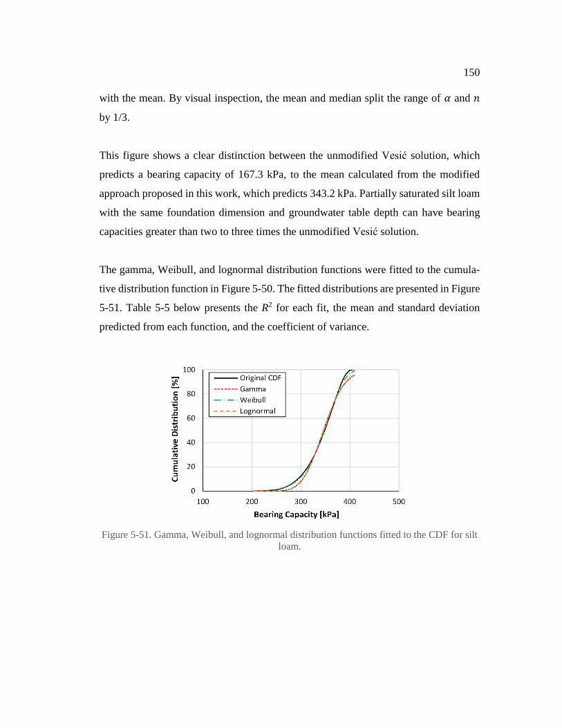
150
with the mean. By visual inspection, the mean and median split the range of 𝛼 and 𝑛
by 1/3.
This figure shows a clear distinction between the unmodified Vesić solution, which
predicts a bearing capacity of 167.3 kPa, to the mean calculated from the modified
approach proposed in this work, which predicts 343.2 kPa. Partially saturated silt loam
with the same foundation dimension and groundwater table depth can have bearing
capacities greater than two to three times the unmodified Vesić solution.
The gamma, Weibull, and lognormal distribution functions were fitted to the cumula-
tive distribution function in Figure 5-50. The fitted distributions are presented in Figure
5-51. Table 5-5 below presents the R2 for each fit, the mean and standard deviation
predicted from each function, and the coefficient of variance.
Figure 5-51. Gamma, Weibull, and lognormal distribution functions fitted to the CDF for silt
loam.

151
Table 5-5. R2, mean, standard deviation, and coefficient of variation predicted from the
Gamma, Weibull, and lognormal distribution functions fitted to silt loam data.
𝑅2 𝜇 (kPa) 𝜎 (kPa) COV (%) Gamma 0.9896 347.3 34.6 10.0 Weibull 0.9988 343.8 35.9 10.4
Lognormal 0.9881 347.7 34.7 9.9
The Weibull distribution function does the best in terms of fitting the measured cumu-
lative distribution function for silt, however, each of the three distribution functions
have reasonable good fits. The predicted mean from the Weibull distribution function
is the closest to the true mean from the Monte Carlo simulations. It can be concluded
that silt loam can be adequately described with a Weibull distribution.
5.5.2. Sand Analysis
Similarly for a sand, the reported average properties for sand are 𝜃𝑠 = 0.43, 𝜃𝑟 =
0.045, 𝑘𝑠 = 8.25 × 10⁻⁵ m/s, 𝛼 = 1.48 kPa−1, and 𝑛 = 2.68. The corresponding
distributions are below:
Figure 5-52. Probability histogram of sand properties used in this work (after Carsel and
Parrish 1988)
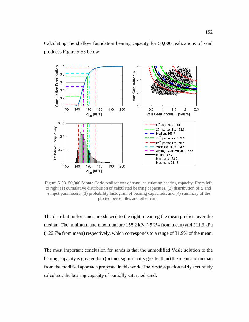
152
Calculating the shallow foundation bearing capacity for 50,000 realizations of sand
produces Figure 5-53 below:
Figure 5-53. 50,000 Monte Carlo realizations of sand, calculating bearing capacity. From left
to right (1) cumulative distribution of calculated bearing capacities, (2) distribution of 𝛼 and
𝑛 input parameters, (3) probability histogram of bearing capacities, and (4) summary of the
plotted percentiles and other data.
The distribution for sands are skewed to the right, meaning the mean predicts over the
median. The minimum and maximum are 158.2 kPa (-5.2% from mean) and 211.3 kPa
(+26.7% from mean) respectively, which corresponds to a range of 31.9% of the mean.
The most important conclusion for sands is that the unmodified Vesić solution to the
bearing capacity is greater than (but not significantly greater than) the mean and median
from the modified approach proposed in this work. The Vesić equation fairly accurately
calculates the bearing capacity of partially saturated sand.

153
The gamma, Weibull, and lognormal distribution functions were also fitted to the CDF
for sand. The fitted distributions are presented in Figure 5-54. Table 5-6 below presents
the R2 for each fit, the mean and standard deviation predicted from each function, and
the coefficient of variance.
Figure 5-54. Gamma, Weibull, and lognormal distribution functions fitted to the CDF for
sand.
Table 5-6. R2, mean, standard deviation, and coefficient of variation predicted from the
Gamma, Weibull, and lognormal distribution functions fitted to sand data.
𝑅2 𝜇 (kPa) 𝜎 (kPa) COV (%) Gamma 0.9870 166.1 4.2 2.5 Weibull 0.9667 165.6 4.6 2.8
Lognormal 0.9874 166.1 4.2 2.5
For sands, both the gamma and lognormal distribution do well in describing the behav-
ior of sands. The predicted mean for the lognormal distribution function is the closest
to the true mean (166.8 kPa) from the Monte Carlo simulations. On this basis, sands
can be most adequately described by the lognormal distribution. It is important to note
that the coefficient of variation is smaller for sands than in silt loams. That implies that
there is greater uncertainty in silt loam unsaturated parameters.

154
5.5.3. Clay Analysis
The reported average properties for clay are 𝜃𝑠 = 0.38, 𝜃𝑟 = 0.068, 𝑘𝑠 = 5.56 ×
10−7 m/s, 𝛼 = 0.082 kPa−1, and 𝑛 = 1.09. The distributions for 𝑘𝑠 and 𝑛 are trun-
cated due to the restriction on these variables. Physically, permeability cannot be less
than 0, and numerically van Genuchten’s n cannot be less than or equal to 1. The fol-
lowing distributions are below:
Figure 5-55. Probability histogram of clay properties used in this work (after Carsel and
Parrish 1988)

155
Figure 5-56. 50,000 Monte Carlo realizations of clay, calculating bearing capacity. From left
to right (1) cumulative distribution of calculated bearing capacities, (2) distribution of 𝛼 and
𝑛 input parameters, (3) probability histogram of bearing capacities, and (4) summary of the
plotted percentiles and other data.
The distribution of the calculated bearing capacity for clays is unlike both silt loam and
sand. Here the bearing capacity distribution is truncated. This is due numerical limita-
tions on the fitting parameter 𝑛, which cannot be less than or equal to 1. The minimum
and maximum calculated bearing capacity is 371.0 kPa (-11.8% from the mean) and
424.1 kPa (+0.8% from the mean), which corresponds to a range of 12.8% from the
mean.
The unmodified Vesić solution calculates a value of 187.7 kPa, which is significantly
lower than the mean and median solution calculated by the modified approach. The
Monte Carlo simulations indicate that this modified method predicts significant, possi-
bly unrealistic, increases in bearing capacity due to partial saturation in clay soils. This

156
significant increase in bearing capacity, relative to sands with the same footing and
friction angle, needs to be assessed physically through model and full-scale footing
tests.
The fitted distributions are presented in Figure 5-57 presents fitted distribution func-
tions for clays. Table 5-7 below presents the R2 for each fit, the mean and standard
deviation predicted from each function, and the coefficient of variance.
Figure 5-57. Gamma, Weibull, and lognormal distribution functions fitted to the CDF for
clay.
Table 5-7. R2, mean, standard deviation, and coefficient of variation predicted from the
Gamma, Weibull, and lognormal distribution functions fitted to clay data.
𝑅2 𝜇 (kPa) 𝜎 (kPa) COV (%) Gamma 0.9609 421.6 2.4 0.6 Weibull 0.9822 421.3 2.6 0.6
Lognormal 0.9608 421.6 2.4 0.6
From Figure 5-57 it is clear that while each distribution function decently describes the
behavior of clay, none of the distribution functions can capture the truncated behavior
at the end of the CDF that is caused by the truncation of 𝑛. It can be concluded from
the 𝑅2 value that Weibull distribution function most adequately describes the variation
of bearing capacity in clays with respect to unsaturated soil properties. Clays had the

157
lowest variation in predicted bearing capacity, followed by sands and silts. This implies
that the unsaturated soils properties for clays had the least variation.
5.6. Discussion
The parametric studies included in this chapter have revealed many interesting behav-
iors for foundations in partially saturated soils. For the shallow foundations, van
Genuchten’s 𝛼 and 𝑛 fitting parameter had the greatest influence on foundation perfor-
mance, varying the magnitude of bearing capacity as well as controlling the shape of
the bearing capacity profile. For 𝛼 and 𝑛 values typical of fine-grained soils, bearing
capacity increased with depth. This was not the case for coarse-grained soils, which
often had a peak bearing capacity at some groundwater table depth. Generally, bearing
capacity increased as 𝛼 and 𝑛 decreased. Another interesting behavior is that the ratio
between the conventional bearing capacity equation and unmodified bearing capacity
equation increased with lower 𝛼 and 𝑛 values. For higher friction angles, this ratio de-
creased.
The 𝛽-method was modified by incorporating suction stresses and by implementing a
new K0 that accounts for tensile stresses in the soil. Tension cracking, which occurs
more predominantly near the surface in fine-grained soils (i.e. small 𝛼 and 𝑛 values),
is a direct by-product of this varied K0. Suction stresses throughout the soil profile,
leads to an increase in side resistance, but is countered by a reduced K0 and tension
cracking near the soil surface. The parametric study on the modified 𝛽-method has
resulted in many interesting conclusions: (1) the selection of low Poisson’s ratio (𝜈 =
0.2) results in more tension cracking, while higher Poisson’s ratios (𝜈 = 0.4) develops
less tension cracking and therefore greater total unit side resistance; (2) tension crack-
ing occurs more frequently in fine-grained soils (low 𝛼 and 𝑛) and will therefore peak
in side resistance as the groundwater table lowers; (3) coarse-grained soils are not con-
trolled by tension cracking and have low suction stresses, therefore side resistance will
continue to increase (to an asymptotic limit) as the groundwater table is lowered; (4)

158
while evaporation increases the suction stress within the soil, it is detrimental to
strength as it increases the depth of cracking; (5) infiltration reduces tension cracking
but also decreases suction stress – soils exposed to infiltration saw a slight increase in
strength from no net flow.
For sands, both the conventional bearing capacity and 𝛽-method generally agreed with
the modified approaches. The inclusion of unsaturated soil mechanics is only signifi-
cant in fine-grained soils such as clays and silts. This behavior is also shown in the
Monte Carlo simulation for sands.
Monte Carlo simulations are an important tool that provide a robust determination of
the confidence bounds for the range of bearing capacity relative to the mean bearing
capacity. These simulations can be further advanced if variation in other soil properties
are well understood (like friction angle, cohesion, and seasonal variation in flux and
groundwater table depth).
The purpose of Monte Carlo simulations in Section 5.5 was to determine typical distri-
butions of unsaturated soil properties and how they might affect the calculated bearing
capacity using the modified approach. In terms of distribution, silts and sands are sim-
ilar but skewed in different directions. The bearing capacity for clays is truncated due
to the numerical limitation placed on the fitting parameter 𝑛. In general, the unmodified
Vesić solution compares well with modified approach used in this work in predicting
the bearing capacity of partially saturated sands.
It has been shown that the Weibull distribution, for silt loam and clays, most adequately
characterizes the variation of bearing capacity with respect to differing unsaturated
properties. For sands, the lognormal distribution sufficiently describes the variation in
bearing capacity. In general, however, the gamma, Weibull, and lognormal distribution
all do well in fitting the results of the Monte Carlo simulation.

159
Another interesting result of these Monte Carlo simulation is the differences in the
range of values. Sands have a range of 31.9% (COV = 2.5%), silt loams 59.4% (COV
= 9.9%), and clays 12.8% (COV = 0.6%) of the mean. Clays have the smallest variation
which indicates that the distribution of unsaturated soil properties does not significantly
affect or change the calculated bearing capacity. Silt loams, which have soil water char-
acteristic curves between sands and clays, have the greatest variation in bearing capac-
ity.

160
6. Conclusions and Future Work
6.1. Conclusions
The purpose of this work was to develop a framework for calculating ultimate bearing
capacity in shallow and deep foundations in partially saturated soils. This theoretical
development included modifying the conventional shallow foundation bearing capacity
equations and the 𝛽-method to incorporate recent literature on unsaturated soil mechan-
ics. Implementation of unsaturated soil mechanics into the conventional bearing capac-
ity equations includes considering apparent cohesion as it varies above the groundwater
table, soil unit weight according to matric suction and the soil water characteristic
curve, and the inclusion of suction stress on overburden. The modified 𝛽-method, has
been designed to include the consideration of suction stress along the drilled shaft and
a reduction of K0 due to tension cracking near the surface. Implementation of these
procedures are discussed in Chapter 3.
The proposed theoretical equation for calculating shallow foundation bearing capacity
has been evaluated with a comparative study of load tests performed on plates and
shallow foundations in partially saturated soils. The modified bearing capacity equa-
tions shows close agreement to measured bearing capacities, having an R2 = 0.81, while
the conventional bearing capacity has very little agreement with the measured data.
This implies that the proposed model for bearing capacity is suitable for use in shallow
foundation design. Based on the load tests considered, the conventional method se-
verely underpredicts the bearing capacity in partially saturated soils and its use may
result in overdesign.
Parametric studies were performed on the modified shallow bearing capacity equation
and modified 𝛽-method for side resistance. For shallow foundations, variation in bear-
ing capacity is most sensitive to the selection of van Genuchten’s 𝛼 and 𝑛 parameters.
In comparing the modified bearing capacity to the convention equational, low values
for 𝛼 and 𝑛 resulted in the highest contrast. Finally, sensitivity to these van Genuchten

161
fitting parameters decreased for larger friction angles. The parametric study for the
modified 𝛽-method showed that side resistance was greatly influenced by tension
cracking, especially for shorter foundations embedded in fine-grained soils. If the
groundwater table was sufficiently deep and the foundation short, tension cracking sig-
nificantly reduced performance. Infiltration generally reduced the depth of tension
cracking, but also reduced the suction stresses in the soil. Evaporation increased the
depth of cracking while increasing suction stresses in the soil. The amount of variation
in suction and cracking was ultimately dependent on material type. Implementation of
Monte Carlo simulations for shallow foundations in partially saturated soils showed
that bearing capacity calculated from silts had the greatest variability, while clays had
the smallest. Finally, for sands, both the conventional bearing capacity equation and
conventional 𝛽-method performed well against the modified approaches.
6.2. Implications for Geotechnical Engineering Practice
The modified shallow foundation bearing capacity equation and 𝛽-method for deep
foundations serve to describe many phenomena in partially saturated soils, especially
in fine-grained soils. As such, it is important to discuss the implication of these pro-
posed methods for use in geotechnical engineering practice.
The proposed shallow foundation bearing capacity equation has shown good agreement
with measured bearing capacity values presented in the literature. This gives some con-
fidence that calculating bearing capacity for partially saturated soils using this approach
may yield suitable bearing capacity values. The database of load tests used in this work
should be expanded in subsequent work to confirm the validity of this approach.
Figure 5-21 is a table of figures that plots contours of the ratio between the bearing
capacity calculated from the modified approach and the conventional Vesić approach.
Within this figure, considerations are made to varying friction angles, ground water

162
table depths, and van Genuchten parameters n and 𝛼. This figure allows for quick esti-
mates of the potential increase (or decrease) of bearing capacity due to partial satura-
tion, especially if the soil texture, grain size distribution, or SWCC are well understood.
The value selected from this figure can be multiplied by the conventional Vesić bearing
capacity equation. For a more robust analysis, Monte Carlo simulations can be con-
ducted, as described in this work, to assess the variability in bearing capacity with re-
spect to unsaturated soil properties. These simulations can also be modified to include
variation in friction angle, steady-state flow, cohesion, saturated water content, and
seasonal variation in the groundwater table depth.
The modified 𝛽-method should be used with caution as no comparison has been made
with measured side resistances of deep foundations. Further, predicted tension cracking
depths from the Lu and Likos (2004) K0 equation and the influence of suction stress on
the soil/foundation interface have not been validated in the literature. Figure 5-41 to
Figure 5-43 plot unit side resistance as a function of Poisson’s ratio, groundwater table
depth, and van Genuchten parameters n and 𝛼. These figures can be used to quickly
estimate the unit side resistance of a deep foundation embedded in partially saturated
soils. While the modified 𝛽-method has not been validated through load testing, it is
useful in assessing whether tension cracking may be an issue or if suction stresses may
contribute to side resistance.
6.3. Future Work
The effects of partial are not typically considered geotechnical engineering applications
such as in foundation design. As a result, there is still a significant amount of research
to be completed on this topic. Shallow and deep foundations design considerations in
partially saturated soils is still lacking in many areas such as settlement. The author has
outlined the following as potential future work for research that pertains to foundation
design in partially saturated soil:
163
- Finite element modeling using the modified Mohr-Coulomb failure criterion or
another unsaturated constitutive model (like the Barcelona Basic Model) in par-
tially saturated soils to assess the impacts of partial saturation on load-displace-
ment behavior.
- Comparison of the modified shallow and deep foundation equations with dif-
ferent definitions for Bishop’s effective stress parameter and different fitting
equations for the soil water characteristic curve.
- Characterization of in-situ matric suction profiles in partially saturated soils,
especially stratified soils. The matric suction profile equation used in this work
is based on the Gardner (1958) hydraulic conductivity model, which has not
been validated in real soils.
- Development of matric suction profile equations in stratified, partially saturated
soils. This work assumes a uniform soil profile since matric suction models in
stratified soils have not been developed.
- Creation of a new matric suction profile equation based off of more recent hy-
draulic conductivity models like Mualem (1976). The matric suction profile
used in this work is based on the Gardner (1958) model.
- Development and application of transient flow equations in partially saturated
soils for shallow and deep foundation bearing capacity. This work assumes
steady-state flow conditions, but this is not reasonable since weather conditions
and water flow are irregular.
- Development of settlement framework/equation for shallow and deep founda-
tions in partially saturated soils. This work only addressed the need for devel-
oping bearing capacity equations for shallow and deep foundations.
- Validation of the modified 𝛽-method through a comparative study on reported
𝛽 coefficients in the literature for normally consolidated, partially saturated
soils.
- The consideration of stress history in the modified 𝛽-method. OCR can be im-
plemented into the modified 𝛽-method to remove the limitation of normally
consolidated soils.

164
- Full-scale shallow foundation load tests in partially saturated soils with a well-
defined soil water characteristic curve, especially in clays. Much of the litera-
ture used in the shallow foundation comparative study was for model footings
loaded on fine sands.
- Development of procedures/standards to measure matric suction during full-
scale load testing. Matric suction measurements should become standard in in-
dustry as it accounts for a considerable amount of strength in fine-grained soils.
The consideration of unsaturated soil mechanics in geotechnical engineering is an im-
portant task. Geotechnical engineering has been plagued with uncertainty, uncertainty
that is continually being reduced. The inclusion of partially saturated soils allows for
more robust designs and a greater understanding of the behavior of soils as a whole.

165
References
Bishop, A. W. (1954). "The Use of Pore Water Coefficients in Practice." Geotechnique,
4, 148-152.
Bishop, A. W. (1959). "The Principle of Effective Stress." Teknisk Ukeblad, 106(39),
859-863.
Briaud, J., and Gibbens, R. (1997). "Large Scale Load Tests and Data Base of Spread
Footings on Sand." Federal Highway Administration.
Briaud, J. L., and Gibbens, R. (1999). "Behavior of Five Large Spread Footings in
Sand." Journal of Geotechnical and Environmental Engineering, 125(9), 787-
796.
Brooks, R. H., and Corey, A. T. (1964). "Hydraulic properties of porous media." Hy-
drology Paper No. 3, Colorado State University.
Burland, J. (1973). "Shaft friction of piles in clay - a simple fundamental approach."
Ground Engineering, 6(3), 30-42.
Burdine, N. T. (1953). "Relative permeability calculations from pore-size distribution
data." Trans. Am. Inst. Min. Eng., 198, 71-78.
Carsel, R. F., and Parrish, R. S. (1988). "Developing Joint Probability Distributions of
Soil Water Retention Characteristics." Water Resources Research, 24(5), 755-
769.
Chen, Y. J., and Kulhawy, F. H. (2002). "Evaluation of Drained Axial Capacity for
Drilled Shafts." Deep Foundations 2002, 256(86), 1200-1214.
Costa, Y. D., Cintra, J. C., and Zornberg, J. G. (2003). "Influence of Matric Suction on
the Results of Plate Load Tests Performed on a Lateritic Soil Deposit." Ge-
otechnical Testing Journal, 26(2), 1-9.
De Beer, E. E. (1970). "Experimental Determination of the Shape Factors and the Bear-
ing Capacity Factors of Sands." Geotechnique, 4, 387-411.
Fellenius, B. H. (2015). Basics of Foundation Design, Sidney, Canada.
Fredlund, D. G., Morgenstern, N. R., and Widger, R. A. (1978). "The Shear Strength
of Unsaturated Soils." Canadian Geotechnical Journal, 15(3), 313-321.
Fredlund, D. G., Rajardjo, H., and Fredlund, M. D. (2012). Unsaturated Soil Mechanics
in Engineering Practice, John Wiley & Sons, New Jersey.
166
Fredlund, D. G., and Xing, A. (1994). "Equations for the soil-water characteristic
curve." Canadian Geotechnical Journal, 31, 521-532.
Fredlund, M. (2011). "SoilVision: Knowledge-Based Soils Database." SoilVision Sys-
tems, Ltd., Saskatoon, Canada.
Gardner, W. R. (1958). "Some Steady State Solutions of the Unsaturated Moisture
Flow Equation with Applications to Evaporation from a Water Table." Soil Sci-
ence, 85(4), 228-232.
Hansen, J. B. (1970). "A Revised and Extended Formula for Bearing Capacity." Ge-
oteknisk Institut, 28, 5-11.
Hansen, J. B. (1970). "A Revised and Extended Formula for Bearing Capacity." Danish
Geotechnical Institute, Bulletin No. 28, 5-11.
Herle, I., and Tejchman, J. "Effects of grain size and pressure level on bearing capacity
of footings on sand." Proc., IS-Nagoya '97, Elsevier Science, 781-786.
Jaky, J. (1948). "Pressure in Silos." Proceedings of the 2nd International Conference
on Soil Mechanics and Foundation Engineering, ICSMFE, London, 103-107.
Khalili, N., and Khabbaz, M. H. (1998). "A Unique Relationship for X for the Deter-
mination of Shear Strength of Unsaturated Soils." Geotechnique, 48(5), 681-
687.
Kondner, R. L. (1963). "A Hyperbolic Stress-Strain Formulation of Sands." Journal of
the Soil and Mechanics and Foundations Division, ASCE, 89(SM1), 115-143.
Kulhawy, F. H., Trautmann, C.H., Beech, J.F., O’Rourke, T.D., McGuire, W., Wood,
W.A., and Capano, C. (1983). "Transmission Line Structure Foundations for
Uplift-Compression Loading." Report EL-2870, Electric Power Research Insti-
tute.
Kumbhojkar, A. S. (1993). "Numerical evaluation of Terzaghi's." Journal of Geotech-
nical and Geoenvironmental Engineering, 119(3), 598-607.
Kusakabe, O. (1995). "Foundations." Geotechnical centrifuge technology, R. N. Tay-
lor, ed. Blackie, London, 443-448.
Larsson, R. (1997). "Investigation and load tests in silty soils." Swedish Geotechnical
Institute, 110-149.
Lu, N., Godt, J. W., and Wu, D. T. (2010). "A Closed-Form Equation for Effective
Stress in Unsaturated Soils." Water Resources Research, 46(W05515).

167
Lu, N., and Griffiths, D. V. (2004). "Profiles of Steady-State Suction Stress in Unsatu-
rated Soils." Journal of Geotechnical and Geoenvironmental Engineering,
130(10), 1063-1076.
Lu, N., Kim, T. K., Stein, S., and Likos, W. J. (2009). "Tensile strength of unsaturated
sand." Journal of Engineering Mechanics, 135(12).
Lu, N., and Likos, W. J. (2004). Unsaturated Soil Mechanics, John Wiley & Sons, Inc.,
Hoboken, New Jersey.
Lu, N., and Likos, W. J. (2006). "Suction Stress Characteristic Curve for Unsaturated
Soil." Journal of Geotechnical and Geoenvironmental Engineering, 132(2),
131-142.
Meyerhof, G.G. (1951). "The Ultimate Bearing Capacity of Foundations." Geotech-
nique, 2(4), 301-332.
Meyerhof, G. G. (1955). "Influence of Roughness of Base and Ground-water Condi-
tions on the Ultimate Bearing Capacity of Foundations." Geotechnique, 5(3),
227-242.
Meyerhof, G.G. (1961). “Discussion on ‘Foundations other than Piled Foundations.’”
Proc. Fifth Int. Conf. Soil Mech., 3, 193.
Meyerhof, G.G. (1963). "Some Recent Research on the Bearing Capacity of Founda-
tions." Canadian Geotechnical Journal, 1(1), 16-26.
Meyerhof, G.G. (1976). "Bearing Capacity and Settlement of Pile Foundations." Jour-
nal of Geotechnical Engineering Division, 102(GT3), 197-228.
Mohamed, F. M. O., and Vanapalli, S. K. (2006). "Laboratory Investigations for the
Measurement of the Bearing Capacity of an Unsaturated Coarse-grained Soil."
Sea to Sky Geotechnique, 219-226.
Mualem, Y. (1976). "A New Model for Predicting the Hydraulic Conductivity of Un-
saturated Porous Media." Water Resources Research, 12(3), 513-522.
O'Neill, M. W. (1987). "Drilled shafts in expansive clays - Design and analysis con-
cepts." Proc., short course on drilled shafts for engineering faculty, ADSC, Dal-
las, Texas.
O'Neill, M. W. (2001). "Side Resistance in Piles and Drilled Shafts." Journal of Ge-
otechnical and Geoenvironmental Engineering, 127(1), 3-16.

168
Oh, W. T., and Vanapalli, S. K. (2008). "Modelling the Stress versus Settlement Be-
havior of Model Footings in Saturated and Unsaturated Sandy Soils." 12th In-
ternational Conference of International Association for Computer Methods and
Advances in Geomechanics. Goa, India, 2126-2137.
Oh, W. T., and Vanapalli, S. K. (2009) "A simple method to estimate the bearing ca-
pacity of unsaturated fine-grained soils." Proc., 62nd Canadian Geotechnical
Conf. & 10th Joint CGS/IAH-CNC Groundwater Conf, 234-241.
Oloo, S. Y., Fredlund, D. G., and Gan, J. K.-M. (1997). "Bearing Capacity of Unpaved
Roads." Canadian Geotechnical Journal, 34, 398-407.
Prandtl, L. (1920). "Über die Härte plasticher Körper." Proc. Kgl. Ges. Wiss. Golt-
ingen, Math. Phys., 74-85.
Reissner, H. (1924). "Zum Erddruckproblem." Proc., 1st Int. Congress for Applied Me-
chanics, 295-311.
Rojas, J. C., Salinas, L. M., and Seja, C. (2007). "Plate-Load Tests on Unsaturated Lean
Clay." Experimental Unsaturated Soil Mechanics, Springer Proceedings in
Physics, 445-452.
Salgado, R. (2008). The Engineering of Foundations, McGraw-Hill, New York.
Skempton, A. W. (1959). "Cast In-situ Bored Piles in London Clay." Geotechnique,
9(4), 153-173.
Steensen-Bach, J. O., Foged, N., and Steenfelt, J. S. (1987). "Capillary induced stresses
- Fact or fiction?" Groundwater Effects in Geotechnical Engineering: Proceed-
ings of the Ninth European Conference on Soil Mechanics and Foundation En-
gineering, 9(1), 83-89.
Terzaghi, K. (1943). Theoretical Soil Mechanics New York, John Wiley and Sons, Inc.
Trautmann, C.H., and Kulhawy, F. H. (1987). "CUFAD-A Computer Program for com-
pression and uplift foundation analysis and design." Report EL-4540-CCM,
vol. 16, Electric Power Research Institute.
United States Department of Agriculture (2016). "USDA Textural Triangle."
Vahedifard, F., and Robinson, J. D. (2015). "Unified method for estimating the ultimate
bearing capacity of shallow foundations in variably saturated soils under steady
flow." Journal of Geotechnical and Geoenvironmental Engineering, 142(4).
van Genuchten, M. T. (1980). "A Closed-form Equation for Predicting the Hydraulic
Conductivity of Unsaturated Soils." Soil Science Society, 44, 892-898.

169
Vanapalli, S. K., and Mohamed, F. M. O. (2007). "Bearing Capacity of Model Footings
in Unsaturated Soils." Proc., Experimental Unsaturated Soil Mechanics,
112(483-493).
Vanapalli, S. K., and Mohamed, F. M. O. (2013). "Bearing Capacity and Settlement of
Footings in Unsaturated Sands." International Journal of Geomaterials, 5(1),
595-604.
Vanapalli, S. K., and Taylan, Z. N. (2011). "Estimation of the Shaft Capacity of Model
Piles in a Compacted Fine-Grained Unsaturated Soil." Proc., Pan-Am CGS Ge-
otechnical Conference.
Vesić, A. (1975). "Analysis of Ultimate Loads of Shallow Foundations." Foundation
Engineering Handbook, Van Nostrand Reinhold Company, ed. by Winterkorn,
H. and Fang, H.Y., 121-147.
Vesić, A. (1973). "Analysis of Ultimate Loads of Shallow Foundations." Journal of the
Soil Mechanics and Foundations Division, 1, 45-71.
Viana da Fonseca, A., and Sousa, J. A. "Hyperbolic Model Parameters for FEM Anal-
ysis of a Footing Load Test on a Residual Soil from Granite - A Database for
Numerical Modelling." Proc., I'ENPC/LCPC, 429-444.
Wuttke, F., Kafle, B., Lins, Y., and Schanz, T. (2013). "Macroelement for Statically
Loaded Shallow Strip Foundation Resting on Unsaturated Soil." International
Journal of Geomechanics, 13(5), 557-564.