unsolved problems in mathematical systems and control
TRANSCRIPT
Unsolved Problems inMathematical Systems andControl Theory
Edited byVincent D. BlondelAlexandre Megretski
PRINCETON UNIVERSITY PRESS
PRINCETON AND OXFORD
iv
Copyright c© 2004 by Princeton University Press
Published by Princeton University Press, 41 William Street, Princeton, NewJersey 08540, USA
In the United Kingdom: Princeton University Press, 3 Market Place, Wood-stock, Oxfordshire OX20 1SY, UK
All rights reserved
Library of Congress Cataloging-in-Publication Data
Unsolved problems in mathematical systems and control theoryEdited by Vincent D. Blondel, Alexandre Megretski. p. cm.Includes bibliographical references.ISBN 0-691-11748-9 (cl : alk. paper)1. System analysis. 2. Control theory. I. Blondel, Vincent. II. Megretski,Alexandre.QA402.U535 2004 2003064802003—dc22
The publisher would like to acknowledge the editors of this volume for pro-viding the camera-ready copy from which this book was printed.
Printed in the United States of America10 9 8 7 6 5 4 3 2 1

I have yet to see any problem, however complicated, which, whenyou looked at it in the right way, did not become still more compli-cated.
Poul Anderson

Contents
Preface xiii
Associate Editors xv
Website xvii
PART 1. LINEAR SYSTEMS 1
Problem 1.1. Stability and composition of transfer functions
Guillermo Fernandez-Anaya, Juan Carlos Martınez-Garcıa 3
Problem 1.2. The realization problem for Herglotz-Nevanlinna functions
Seppo Hassi, Henk de Snoo, Eduard Tsekanovskiı 8
Problem 1.3. Does any analytic contractive operator function on the polydisk
have a dissipative scattering nD realization?
Dmitry S. Kalyuzhniy-Verbovetzky 14
Problem 1.4. Partial disturbance decoupling with stability
Juan Carlos Martınez-Garcıa, Michel Malabre, Vladimir Kucera 18
Problem 1.5. Is Monopoli’s model reference adaptive controller correct?
A. S. Morse 22
Problem 1.6. Model reduction of delay systems
Jonathan R. Partington 29
Problem 1.7. Schur extremal problems
Lev Sakhnovich 33
Problem 1.8. The elusive iff test for time-controllability of behaviors
Amol J. Sasane 36
viii CONTENTS
Problem 1.9. A Farkas lemma for behavioral inequalities
A.A. (Tonny) ten Dam, J.W. (Hans) Nieuwenhuis 40
Problem 1.10. Regular feedback implementability of linear differential behaviors
H. L. Trentelman 44
Problem 1.11. Riccati stability
Erik I. Verriest 49
Problem 1.12. State and first order representations
Jan C. Willems 54
Problem 1.13. Projection of state space realizations
Antoine Vandendorpe, Paul Van Dooren 58
PART 2. STOCHASTIC SYSTEMS 65
Problem 2.1. On error of estimation and minimum of cost for wide band noise
driven systems
Agamirza E. Bashirov 67
Problem 2.2. On the stability of random matrices
Giuseppe C. Calafiore, Fabrizio Dabbene 71
Problem 2.3. Aspects of Fisher geometry for stochastic linear systems
Bernard Hanzon, Ralf Peeters 76
Problem 2.4. On the convergence of normal forms for analytic control systems
Wei Kang, Arthur J. Krener 82
PART 3. NONLINEAR SYSTEMS 87
Problem 3.1. Minimum time control of the Kepler equation
Jean-Baptiste Caillau, Joseph Gergaud, Joseph Noailles 89
Problem 3.2. Linearization of linearly controllable systems
R. Devanathan 93
Problem 3.3. Bases for Lie algebras and a continuous CBH formula
Matthias Kawski 97
CONTENTS ix
Problem 3.4. An extended gradient conjecture
Luis Carlos Martins Jr., Geraldo Nunes Silva 103
Problem 3.5. Optimal transaction costs from a Stackelberg perspective
Geert Jan Olsder 107
Problem 3.6. Does cheap control solve a singular nonlinear quadratic problem?
Yuri V. Orlov 111
Problem 3.7. Delta-Sigma modulator synthesis
Anders Rantzer 114
Problem 3.8. Determining of various asymptotics of solutions of nonlinear time-
optimal problems via right ideals in the moment algebra
G. M. Sklyar, S. Yu. Ignatovich 117
Problem 3.9. Dynamics of principal and minor component flows
U. Helmke, S. Yoshizawa, R. Evans, J.H. Manton, and I.M.Y. Mareels 122
PART 4. DISCRETE EVENT, HYBRID SYSTEMS 129
Problem 4.1. L2-induced gains of switched linear systems
Joao P. Hespanha 131
Problem 4.2. The state partitioning problem of quantized systems
Jan Lunze 134
Problem 4.3. Feedback control in flowshops
S.P. Sethi and Q. Zhang 140
Problem 4.4. Decentralized control with communication between controllers
Jan H. van Schuppen 144
PART 5. DISTRIBUTED PARAMETER SYSTEMS 151
Problem 5.1. Infinite dimensional backstepping for nonlinear parabolic PDEs
Andras Balogh, Miroslav Krstic 153
Problem 5.2. The dynamical Lame system with boundary control: on the struc-
ture of reachable sets
M.I. Belishev 160
x CONTENTS
Problem 5.3. Null-controllability of the heat equation in unbounded domains
Sorin Micu, Enrique Zuazua 163
Problem 5.4. Is the conservative wave equation regular?
George Weiss 169
Problem 5.5. Exact controllability of the semilinear wave equation
Xu Zhang, Enrique Zuazua 173
Problem 5.6. Some control problems in electromagnetics and fluid dynamics
Lorella Fatone, Maria Cristina Recchioni, Francesco Zirilli 179
PART 6. STABILITY, STABILIZATION 187
Problem 6.1. Copositive Lyapunov functions
M. K. Camlıbel, J. M. Schumacher 189
Problem 6.2. The strong stabilization problem for linear time-varying systems
Avraham Feintuch 194
Problem 6.3. Robustness of transient behavior
Diederich Hinrichsen, Elmar Plischke, Fabian Wirth 197
Problem 6.4. Lie algebras and stability of switched nonlinear systems
Daniel Liberzon 203
Problem 6.5. Robust stability test for interval fractional order linear systems
Ivo Petras, YangQuan Chen, Blas M. Vinagre 208
Problem 6.6. Delay-independent and delay-dependent Aizerman problem
Vladimir Rasvan 212
Problem 6.7. Open problems in control of linear discrete multidimensional sys-
tems
Li Xu, Zhiping Lin, Jiang-Qian Ying, Osami Saito, Yoshihisa Anazawa 221
Problem 6.8. An open problem in adaptative nonlinear control theory
Leonid S. Zhiteckij 229
Problem 6.9. Generalized Lyapunov theory and its omega-transformable regions
Sheng-Guo Wang 233
CONTENTS xi
Problem 6.10. Smooth Lyapunov characterization of measurement to error sta-
bility
Brian P. Ingalls, Eduardo D. Sontag 239
PART 7. CONTROLLABILITY, OBSERVABILITY 245
Problem 7.1. Time for local controllability of a 1-D tank containing a fluid
modeled by the shallow water equations
Jean-Michel Coron 247
Problem 7.2. A Hautus test for infinite-dimensional systems
Birgit Jacob, Hans Zwart 251
Problem 7.3. Three problems in the field of observability
Philippe Jouan 256
Problem 7.4. Control of the KdV equation
Lionel Rosier 260
PART 8. ROBUSTNESS, ROBUST CONTROL 265
Problem 8.1. H∞-norm approximation
A.C. Antoulas, A. Astolfi 267
Problem 8.2. Noniterative computation of optimal value in H∞ control
Ben M. Chen 271
Problem 8.3. Determining the least upper bound on the achievable delay margin
Daniel E. Davison, Daniel E. Miller 276
Problem 8.4. Stable controller coefficient perturbation in floating point imple-
mentation
Jun Wu, Sheng Chen 280
PART 9. IDENTIFICATION, SIGNAL PROCESSING 285
Problem 9.1. A conjecture on Lyapunov equations and principal angles in sub-
space identification
Katrien De Cock, Bart De Moor 287
xii CONTENTS
Problem 9.2. Stability of a nonlinear adaptive system for filtering and parameter
estimation
Masoud Karimi-Ghartemani, Alireza K. Ziarani 293
PART 10. ALGORITHMS, COMPUTATION 297
Problem 10.1. Root-clustering for multivariate polynomials and robust stability
analysis
Pierre-Alexandre Bliman 299
Problem 10.2. When is a pair of matrices stable?
Vincent D. Blondel, Jacques Theys, John N. Tsitsiklis 304
Problem 10.3. Freeness of multiplicative matrix semigroups
Vincent D. Blondel, Julien Cassaigne, Juhani Karhumaki 309
Problem 10.4. Vector-valued quadratic forms in control theory
Francesco Bullo, Jorge Cortes, Andrew D. Lewis, Sonia Martınez 315
Problem 10.5. Nilpotent bases of distributions
Henry G. Hermes, Matthias Kawski 321
Problem 10.6. What is the characteristic polynomial of a signal flow graph?
Andrew D. Lewis 326
Problem 10.7. Open problems in randomized µ analysis
Onur Toker 330
Preface
Five years ago, a first volume of open problems in Mathematical Systemsand Control Theory appeared.1 Some of the 53 problems that were publishedin this volume attracted considerable attention in the research community.
The book in front of you contains a new collection of 63 open problems.The contents of both volumes show the evolution of the field in the halfdecade since the publication of the first volume. One noticeable feature isthe shift toward a wider class of questions and more emphasis on issuesdriven by physical modeling.
Early versions of some of the problems in this book have been presented atthe Open Problem sessions of the Oberwolfach Tagung on Regelungstheorie,on February 27, 2002, and of the Conference on Mathematical Theory ofNetworks and Systems (MTNS) in Notre Dame, Indiana, on August 12, 2002.The editors thank the organizers of these meetings for their willingness toprovide the problems this welcome exposure.
Since the appearance of the first volume, open problems have continuedto meet with large interest in the mathematical community. Undoubtedly,the most spectacular event in this arena was the announcement by the ClayMathematics Institute2 of the Millennium Prize Problems whose solutionwill be rewarded by one million U.S. dollars each. Modesty and modesty ofmeans have prevented the editors of the present volume from offering similarrewards toward the solution of the problems in this book. However, we trustthat, notwithstanding this absence of a financial incentive, the intellectualchallenge will stimulate many readers to attack the problems.
The editors thank in the first place the researchers who have submittedthe problems. We are also very thankful to the Princeton University Press,and in particular Vickie Kearn, for their willingness to publish this vol-ume. The full text of the problems, together with comments, additions,and solutions, will be posted on the book website at Princeton Univer-sity Press (link available from http://pup.princeton.edu/math/) and onhttp://www.inma.ucl.ac.be/∼blondel/op/. Readers are encouraged tosubmit contributions by following the instructions given on these websites.
The editors, Louvain-la-Neuve, March 15, 2003.
1Vincent D. Blondel, Eduardo D. Sontag, M. Vidyasagar, and Jan C. Willems, OpenProblems in Mathematical Systems and Control Theory, Springer Verlag, 1998.
2See http://www.claymath.org.

Associate Editors
Roger Brockett, Harvard University, USAJean-Michel Coron, University of Paris (Orsay), FranceRoland Hildebrand, University of Louvain (Louvain-la-Neuve), BelgiumMiroslav Krstic, University of California (San Diego), USAAnders Rantzer, Lund Institute of Technology, SwedenJoachim Rosenthal, University of Notre Dame, USAEduardo Sontag, Rutgers University, USAM. Vidyasagar, Tata Consultancy Services, IndiaJan Willems, University of Leuven, Belgium


Website
The full text of the problems presented in this book, together with com-ments, additions and solutions, are freely available in electronic format fromthe book website at Princeton University Press:
http://pup.princeton.edu/math/
and from an editor website:
http://www.inma.ucl.ac.be/∼blondel/op/
Readers are encouraged to submit contributions by following the instruc-tions given on these websites.


PART 1
Linear Systems

Problem 1.1
Stability and composition of transfer functions
G. Fernandez-AnayaDepartamento de Ciencias BasicasUniversidad IberoamericanaLomas de Santa Fe01210 Mexico [email protected]
J. C. Martınez-GarcıaDepartamento de Control AutomaticoCINVESTAV-IPNA.P. 14-74007300 Mexico [email protected]
1 INTRODUCTION
As far as the frequency-described continuous linear time-invariant systemsare concerned, the study of control-oriented properties (like stability) re-sulting from the substitution of the complex Laplace variable s by rationaltransfer functions have been little studied by the Automatic Control com-munity. However, some interesting results have recently been published:Concerning the study of the so-called uniform systems, i.e., LTI systemsconsisting of identical components and amplifiers, it was established in [8]a general criterion for robust stability for rational functions of the formD(f(s)), where D(s) is a polynomial and f(s) is a rational transfer function.By applying such a criterium, it gave a generalization of the celebratedKharitonov’s theorem [7], as well as some robust stability criteria under H∞-uncertainty. The results given in [8] are based on the so-called H-domains.1
As far as robust stability of polynomial families is concerned, some Kharito-
1The H-domain of a function f (s) is defined to be the set of points h on the complexplane for which the function f (s)− h has no zeros on the open right-half complex plane.
4 PROBLEM 1.1
nov’s like results [7] are given in [9] (for a particular class of polynomials),when interpreting substitutions as nonlinearly correlated perturbations onthe coefficients.More recently, in [1], some results for proper and stable real rational SISOfunctions and coprime factorizations were proved, by making substitutionswith α (s) = (as+ b) / (cs+ d), where a, b, c, and d are strictly positive realnumbers, and with ad− bc 6= 0. But these results are limited to the bilineartransforms, which are very restricted.In [4] is studied the preservation of properties linked to control problems (likeweighted nominal performance and robust stability) for Single-Input Single-Output systems, when performing the substitution of the Laplace variable (intransfer functions associated to the control problems) by strictly positive realfunctions of zero relative degree. Some results concerning the preservation ofcontrol-oriented properties in Multi-Input Multi-Output systems are given in[5], while [6] deals with the preservation of solvability conditions in algebraicRiccati equations linked to robust control problems.Following our interest in substitutions we propose in section 22.2 three in-teresting problems. The motivations concerning the proposed problems arepresented in section 22.3.
2 DESCRIPTION OF THE PROBLEMS
In this section we propose three closely related problems. The first one con-cerns the characterization of a transfer function as a composition of transferfunctions. The second problem is a modified version of the first problem:the characterization of a transfer function as the result of substituting theLaplace variable in a transfer function by a strictly positive real transferfunction of zero relative degree. The third problem is in fact a conjectureconcerning the preservation of stability property in a given polynomial re-sulting from the substitution of the coefficients in the given polynomial bya polynomial with non-negative coefficients evaluated in the substituted co-efficients.
Problem 1: Let a Single Input Single Output (SISO) transfer function G(s)be given. Find transfer functions G0(s) and H(s) such that:
1. G (s) = G0 (H (s)) ;
2. H (s) preserves proper stable transfer functions under substitution ofthe variable s by H (s), and:
3. The degree of the denominator of H(s) is the maximum with the prop-erties 1 and 2.
STABILITY AND COMPOSITION OF TRANSFER FUNCTIONS 5
Problem 2: Let a SISO transfer function G(s) be given. Find a transferfunction G0 (s) and a Strictly Positive Real transfer function of zero relativedegree (SPR0), say H(s), such that:
1. G(s) = G0 (H (s)) and:
2. The degree of the denominator of H(s) is the maximum with the prop-erty 1.
Problem 3: (Conjecture) Given any stable polynomial:
ansn + an−1s
n−1 + · · ·+ a1s+ a0
and given any polynomial q(s) with non-negative coefficients, then the poly-nomial:
q(an)sn + q(an−1)sn−1 + · · ·+ q(a1)s+ q(a0)
is stable (see [3]).
3 MOTIVATIONS
Consider the closed-loop control scheme:
y (s) = G (s)u (s) + d (s) , u (s) = K (s) (r (s)− y (s)) ,
where: P (s) denotes the SISO plant; K (s) denotes a stabilizing controller;u (s) denotes the control input; y (s) denotes the control input; d (s) denotesthe disturbance and r (s) denotes the reference input. We shall denote theclosed-loop transfer function from r (s) to y (s) as Fr (G (s) ,K (s)) and theclosed-loop transfer function from d (s) to y (s) as Fd (G (s) ,K (s)).
• Consider the closed-loop system Fr (G (s) ,K (s)), and suppose thatthe plant G(s) results from a particular substitution of the s Laplacevariable in a transfer function G0(s) by a transfer function H(s),i.e., G(s) = G0(H(s)). It has been proved that a controller K0 (s)which stabilizes the closed-loop system Fr (G0 (s) ,K0 (s)) is such thatK0 (H (s)) stabilizes Fr (G (s) ,K0 (H (s))) (see [2] and [8]). Thus, thesimplification of procedures for the synthesis of stabilizing controllers(profiting from transfer function compositions) justifies problem 1.
• As far as problem 2 is concerned, consider the synthesis of a controllerK (s) stabilizing the closed-loop transfer function Fd (G (s) ,K (s)),and such that ‖Fd (G (s) ,K (s))‖∞ < γ, for a fixed given γ > 0. If weknown that G(s) = G0 (H (s)), being H (s) a SPR0 transfer function,the solution of problem 2 would arise to the following procedure:
1. Find a controller K0(s) which stabilizes the closed-loop transferfunction Fd (G0 (s) ,K0 (s)) and such that:
‖Fd (G0 (s) ,K0 (s))‖∞ < γ.
6 PROBLEM 1.1
2. The composed controller K (s) = K0 (H (s)) stabilizes the closed-loop system Fd (G (s) ,K (s)) and:
‖Fd (G (s) ,K (s))‖∞ < γ
(see [2], [4], and [5]).
It is clear that condition 3 in the first problem, or condition 2 inthe second problem, can be relaxed to the following condition: thedegree of the denominator of H (s) is as high as be possible withthe appropriate conditions. With this new condition, the openproblems are a bit less difficult.
• Finally, problem 3 can be interpreted in terms of robustness underpositive polynomial perturbations in the coefficients of a stable transferfunction.
BIBLIOGRAPHY
[1] G. Fernandez, S. Munoz, R. A. Sanchez, and W. W. Mayol, “Simulta-neous stabilization using evolutionary strategies,”Int. J. Contr., vol. 68,no. 6, pp. 1417-1435, 1997.
[2] G. Fernandez, “Preservation of SPR functions and stabilization by sub-stitutions in SISO plants,”IEEE Transaction on Automatic Control, vol.44, no. 11, pp. 2171-2174, 1999.
[3] G. Fernandez and J. Alvarez, “On the preservation of stability in fam-ilies of polynomials via substitutions,”Int. J. of Robust and NonlinearControl, vol. 10, no. 8, pp. 671-685, 2000.
[4] G. Fernandez, J. C. Martınez-Garcıa, and V. Kucera, “H∞-RobustnessProperties Preservation in SISO Systems when applying SPR Substitu-tions,”Submitted to the International Journal of Automatic Control.
[5] G. Fernandez and J. C. Martınez-Garcıa, “MIMO Systems PropertiesPreservation under SPR Substitutions,” International Symposium on theMathematical Theory of Networks and Systems (MTNS’2002), Universityof Notre Dame, USA, August 12-16, 2002.
[6] G. Fernandez, J. C. Martınez-Garcıa, and D. Aguilar-George, “Preserva-tion of solvability conditions in Riccati equations when applying SPR0substitutions,” submitted to IEEE Transactions on Automatic Control,2002.
[7] V. L. Kharitonov, “Asymptotic stability of families of systems of lineardifferential equations, ”Differential’nye Uravneniya, vol. 14, pp. 2086-2088, 1978.
STABILITY AND COMPOSITION OF TRANSFER FUNCTIONS 7
[8] B. T. Polyak and Ya. Z. Tsypkin, “Stability and robust stability of uni-form systems, ”Automation and Remote Contr., vol. 57, pp. 1606-1617,1996.
[9] L. Wang, “Robust stability of a class of polynomial families under non-linearly correlated perturbations,”System and Control Letters, vol. 30,pp. 25-30, 1997.
Problem 1.2
The realization problem for Herglotz-Nevanlinna
functions
Seppo HassiDepartment of Mathematics and StatisticsUniversity of VaasaP.O. Box 700, 65101 [email protected]
Henk de SnooDepartment of MathematicsUniversity of GroningenP.O. Box 800, 9700 AV [email protected]
Eduard TsekanovskiıDepartment of MathematicsNiagara University, NY [email protected]
1 MOTIVATION AND HISTORY OF THE PROBLEM
Roughly speaking, realization theory concerns itself with identifying a givenholomorphic function as the transfer function of a system or as its linear frac-tional transformation. Linear, conservative, time-invariant systems whosemain operator is bounded have been investigated thoroughly. However, manyrealizations in different areas of mathematics including system theory, elec-trical engineering, and scattering theory involve unbounded main operators,and a complete theory is still lacking. The aim of the present proposal isto outline the necessary steps needed to obtain a general realization theoryalong the lines of M. S. Brodskiı and M. S. Livsic [8], [9], [16], who have
THE REALIZATION PROBLEM FOR HERGLOTZ-NEVANLINNA FUNCTIONS 9
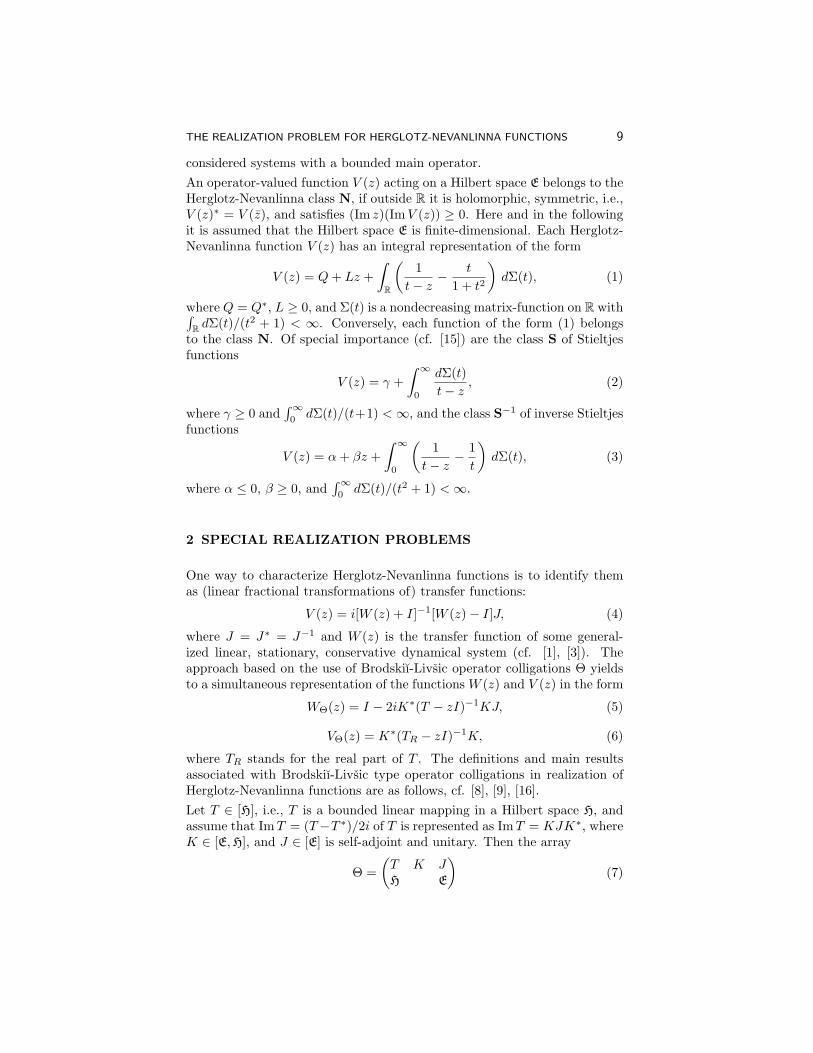
considered systems with a bounded main operator.An operator-valued function V (z) acting on a Hilbert space E belongs to theHerglotz-Nevanlinna class N, if outside R it is holomorphic, symmetric, i.e.,V (z)∗ = V (z), and satisfies (Im z)(ImV (z)) ≥ 0. Here and in the followingit is assumed that the Hilbert space E is finite-dimensional. Each Herglotz-Nevanlinna function V (z) has an integral representation of the form
V (z) = Q+ Lz +∫
R
(1
t− z− t
1 + t2
)dΣ(t), (1)
where Q = Q∗, L ≥ 0, and Σ(t) is a nondecreasing matrix-function on R with∫R dΣ(t)/(t2 + 1) < ∞. Conversely, each function of the form (1) belongs
to the class N. Of special importance (cf. [15]) are the class S of Stieltjesfunctions
V (z) = γ +∫ ∞
0
dΣ(t)t− z
, (2)
where γ ≥ 0 and∫∞0dΣ(t)/(t+1) <∞, and the class S−1 of inverse Stieltjes
functions
V (z) = α+ βz +∫ ∞
0
(1
t− z− 1t
)dΣ(t), (3)
where α ≤ 0, β ≥ 0, and∫∞0dΣ(t)/(t2 + 1) <∞.
2 SPECIAL REALIZATION PROBLEMS
One way to characterize Herglotz-Nevanlinna functions is to identify themas (linear fractional transformations of) transfer functions:
V (z) = i[W (z) + I]−1[W (z)− I]J, (4)
where J = J∗ = J−1 and W (z) is the transfer function of some general-ized linear, stationary, conservative dynamical system (cf. [1], [3]). Theapproach based on the use of Brodskiı-Livsic operator colligations Θ yieldsto a simultaneous representation of the functions W (z) and V (z) in the form
WΘ(z) = I − 2iK∗(T − zI)−1KJ, (5)
VΘ(z) = K∗(TR − zI)−1K, (6)
where TR stands for the real part of T . The definitions and main resultsassociated with Brodskiı-Livsic type operator colligations in realization ofHerglotz-Nevanlinna functions are as follows, cf. [8], [9], [16].Let T ∈ [H], i.e., T is a bounded linear mapping in a Hilbert space H, andassume that ImT = (T−T ∗)/2i of T is represented as ImT = KJK∗, whereK ∈ [E,H], and J ∈ [E] is self-adjoint and unitary. Then the array
Θ =(T K JH E
)(7)
10 PROBLEM 1.2
defines a Brodskiı-Livsic operator colligation, and the function WΘ(z) givenby (5) is the transfer function of Θ. In the case of the directing operatorJ = I the system (7) is called a scattering system, in which case the mainoperator T of the system Θ is dissipative: ImT ≥ 0. In system theoryWΘ(z) is interpreted as the transfer function of the conservative system(i.e., ImT = KJK∗) of the form (T −zI)x = KJϕ− and ϕ+ = ϕ−−2iK∗x,where ϕ− ∈ E is an input vector, ϕ+ ∈ E is an output vector, and x isa state space vector in H, so that ϕ+ = WΘ(z)ϕ−. The system is said tobe minimal if the main operator T of Θ is completely non self-adjoint (i.e.,there are no nontrivial invariant subspaces on which T induces self-adjointoperators), cf. [8], [16]. A classical result due to Brodskiı and Livsic [9]states that the compactly supported Herglotz-Nevanlinna functions of theform
∫ badΣ(t)/(t− z) correspond to minimal systems Θ of the form (7) via
(4) with W (z) = WΘ(z) given by (5) and V (z) = VΘ(z) given by (6).Next consider a linear, stationary, conservative dynamical system Θ of theform
Θ =(
A K JH+ ⊂ H ⊂ H− E
). (8)
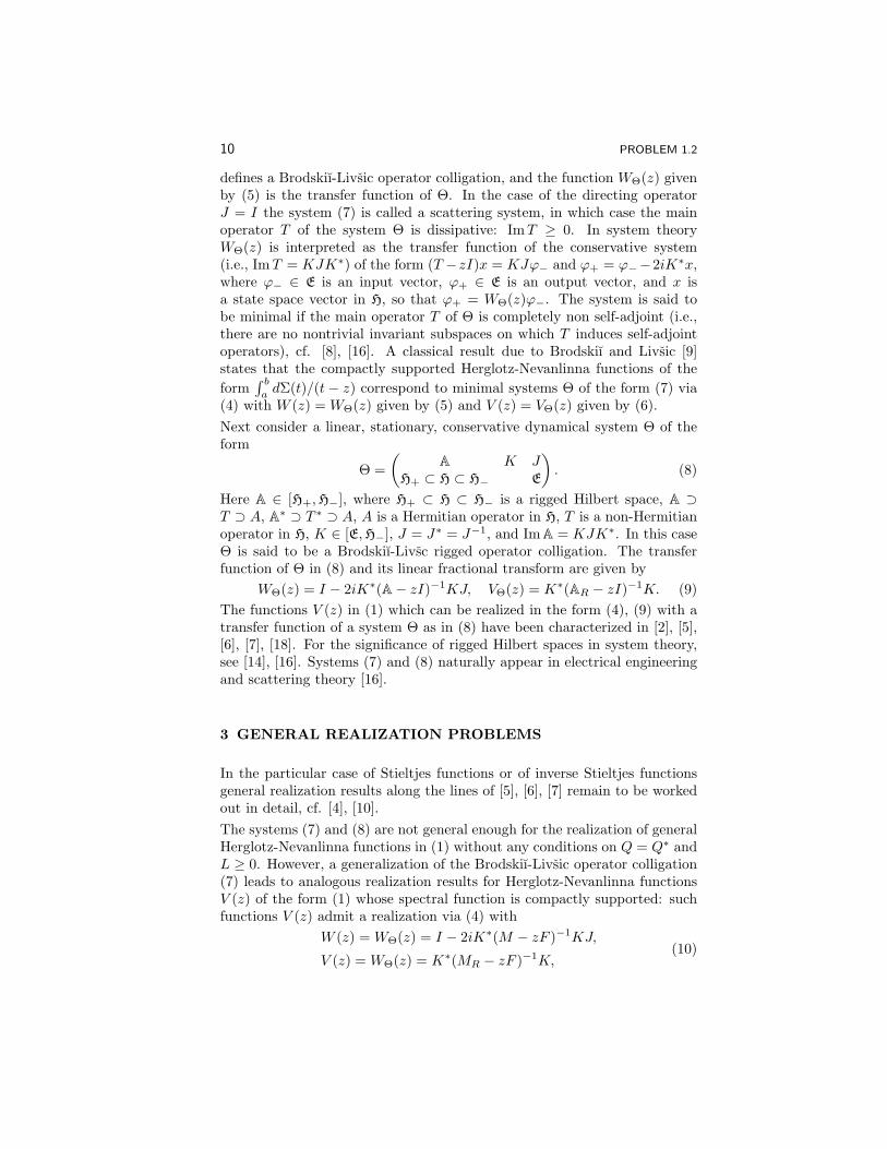
Here A ∈ [H+,H−], where H+ ⊂ H ⊂ H− is a rigged Hilbert space, A ⊃T ⊃ A, A∗ ⊃ T ∗ ⊃ A, A is a Hermitian operator in H, T is a non-Hermitianoperator in H, K ∈ [E,H−], J = J∗ = J−1, and Im A = KJK∗. In this caseΘ is said to be a Brodskiı-Livsc rigged operator colligation. The transferfunction of Θ in (8) and its linear fractional transform are given by
WΘ(z) = I − 2iK∗(A− zI)−1KJ, VΘ(z) = K∗(AR − zI)−1K. (9)The functions V (z) in (1) which can be realized in the form (4), (9) with atransfer function of a system Θ as in (8) have been characterized in [2], [5],[6], [7], [18]. For the significance of rigged Hilbert spaces in system theory,see [14], [16]. Systems (7) and (8) naturally appear in electrical engineeringand scattering theory [16].
3 GENERAL REALIZATION PROBLEMS
In the particular case of Stieltjes functions or of inverse Stieltjes functionsgeneral realization results along the lines of [5], [6], [7] remain to be workedout in detail, cf. [4], [10].The systems (7) and (8) are not general enough for the realization of generalHerglotz-Nevanlinna functions in (1) without any conditions on Q = Q∗ andL ≥ 0. However, a generalization of the Brodskiı-Livsic operator colligation(7) leads to analogous realization results for Herglotz-Nevanlinna functionsV (z) of the form (1) whose spectral function is compactly supported: suchfunctions V (z) admit a realization via (4) with
W (z) = WΘ(z) = I − 2iK∗(M − zF )−1KJ,
V (z) = WΘ(z) = K∗(MR − zF )−1K,(10)

THE REALIZATION PROBLEM FOR HERGLOTZ-NEVANLINNA FUNCTIONS 11
where M = MR + iKJK∗, MR ∈ [H] is the real part of M , F is a finite-dimensional orthogonal projector, and Θ is a generalized Brodskiı-Livsicoperator colligation of the form
Θ =(M F K J
H E
), (11)
see [11], [12], [13]. The basic open problems are:
Determine the class of linear, conservative, time-invariant dynamical sys-tems (new type of operator colligations) such that an arbitrary matrix-valuedHerglotz-Nevanlinna function V (z) acting on E can be realized as a linearfractional transformation (4) of the matrix-valued transfer function WΘ(z)of some minimal system Θ from this class.
Find criteria for a given matrix-valued Stieltjes or inverse Stieltjes functionacting on E to be realized as a linear fractional transformation of the matrix-valued transfer function of a minimal Brodskiı-Livsic type system Θ in (8)with: (i) an accretive operator A, (ii) an α-sectorial operator A, or (iii) anextremal operator A (accretive but not α-sectorial).
The same problem for the (compactly supported) matrix-valued Stieltjes orinverse Stieltjes functions and the generalized Brodskiı-Livsic systems of theform (11) with the main operator M and the finite-dimensional orthogonalprojector F .
There is a close connection to the so-called regular impedance conserva-tive systems (where the coefficient of the derivative is invertible) that wererecently considered in [17] (see also [19]). It is shown that any functionD(s) with non-negative real part in the open right half-plane and for whichD(s)/s→ 0 as s→∞ has a realization with such an impedance conservativesystem.
BIBLIOGRAPHY
[1] D. Alpay, A. Dijksma, J. Rovnyak, and H.S.V. de Snoo, “Schur func-tions, operator colligations, and reproducing kernel Pontryagin spaces,”Oper. Theory Adv. Appl., 96, Birkhauser Verlag, Basel, 1997.
[2] Yu. M. Arlinskiı, “On the inverse problem of the theory of characteristicfunctions of unbounded operator colligations”, Dopovidi Akad. NaukUkrain. RSR, 2 (1976), 105–109 (Russian).
[3] D. Z. Arov, “Passive linear steady-state dynamical systems,” Sibirsk.Mat. Zh., 20, no. 2, (1979), 211–228, 457 (Russian) [English transl.:Siberian Math. J., 20 no. 2, (1979) 149–162].
12 PROBLEM 1.2
[4] S. V. Belyi, S. Hassi, H. S. V. de Snoo, and E. R. Tsekanovskiı,“On the realization of inverse Stieltjes functions,” Proceedingsof the 15th International Symposium on Mathematical Theory ofNetworks and Systems, Editors D. Gillian and J. Rosenthal,University of Notre Dame, South Bend, Idiana, USA, 2002,http://www.nd.edu/∼mtns/papers/20160 6.pdf
[5] S. V. Belyi and E. R. Tsekanovskiı, “Realization and factorization prob-lems for J-contractive operator-valued functions in half-plane and sys-tems with unbounded operators,” Systems and Networks: Mathemati-cal Theory and Applications, Akademie Verlag, 2 (1994), 621–624.
[6] S. V. Belyi and E. R. Tsekanovskiı, “Realization theorems for operator-valued R-functions,” Oper. Theory Adv. Appl., 98 (1997), 55–91.
[7] S. V. Belyi and E. R. Tsekanovskiı, “On classes of realizable operator-valued R-functions,” Oper. Theory Adv. Appl., 115 (2000), 85–112.
[8] M. S. Brodskiı, “Triangular and Jordan representations of linear op-erators,” Moscow, Nauka, 1969 (Russian) [English trans.: Vol. 32 ofTransl. Math. Monographs, Amer. Math. Soc., 1971].
[9] M. S. Brodskiı and M. S. Livsic, “Spectral analysis of non-selfadjointoperators and intermediate systems,” Uspekhi Mat. Nauk, 13 no. 1, 79,(1958), 3–85 (Russian) [English trans.: Amer. Math. Soc. Transl., (2)13 (1960), 265–346].
[10] I. Dovshenko and E. R.Tsekanovskiı, “Classes of Stieltjes operator-functions and their conservative realizations,” Dokl. Akad. Nauk SSSR,311 no. 1 (1990), 18–22.
[11] S. Hassi, H. S. V. de Snoo, and E. R. Tsekanovskiı, “An addendumto the multiplication and factorization theorems of Brodskiı-Livsic-Potapov,” Appl. Anal., 77 (2001), 125–133.
[12] S. Hassi, H. S. V. de Snoo, and E. R. Tsekanovskiı, “On commuta-tive and noncommutative representations of matrix-valued Herglotz-Nevanlinna functions,” Appl. Anal., 77 (2001), 135–147.
[13] S. Hassi, H. S. V. de Snoo, and E. R. Tsekanovskiı, “Realizationsof Herglotz-Nevanlinna functions via F -systems,” Oper. Theory: Adv.Appl., 132 (2002), 183–198.
[14] J.W. Helton, “Systems with infinite-dimensional state space: theHilbert space approach,” Proc. IEEE, 64 (1976), no. 1, 145–160.
[15] I. S. Kac and M. G. Kreın, “The R-functions: Analytic functions map-ping the upper half-plane into itself,” Supplement I to the Russian edi-tion of F. V. Atkinson, Discrete and Continuous Boundary Problems,Moscow, 1974 [English trans.: Amer. Math. Soc. Trans., (2) 103 (1974),1–18].
THE REALIZATION PROBLEM FOR HERGLOTZ-NEVANLINNA FUNCTIONS 13
[16] M. S. Livsic, “Operators, Oscillations, Waves,” Moscow, Nauka, 1966(Russian) [English trans.: Vol. 34 of Trans. Math. Monographs, Amer.Math. Soc., 1973].
[17] O. J. Staffans, “Passive and conservative infinite-dimensionalimpedance and scattering systems (from a personal point of view),” Pro-ceedings of the 15th International Symposium on Mathematical Theoryof Networks and Systems, Ed., D. Gillian and J. Rosenthal, Univer-sity of Notre Dame, South Bend, Indiana, USA, 2002, Plenary talk,http://www.nd.edu/∼mtns
[18] E. R. Tsekanovskiı and Yu. L. Shmul’yan, “The theory of biextensionsof operators in rigged Hilbert spaces: Unbounded operator colligationsand characteristic functions,” Uspekhi Mat. Nauk, 32 (1977), 69–124(Russian) [English transl.: Russian Math. Surv., 32 (1977), 73–131].
[19] G. Weiss, “Transfer functions of regular linear systems. Part I: charac-terizations of regularity”, Trans. Amer. Math. Soc., 342 (1994), 827–854.
Problem 1.3
Does any analytic contractive operator function on
the polydisk have a dissipative scattering nD
realization?
Dmitry S. Kalyuzhniy-VerbovetzkyDepartment of MathematicsThe Weizmann Institute of ScienceRehovot [email protected]
1 DESCRIPTION OF THE PROBLEM
Let X,U,Y be finite-dimensional or infinite-dimensional separable Hilbertspaces. Consider nD linear systems of the form
α :
x(t) =
n∑k=1
(Akx(t− ek) +Bku(t− ek)),
y(t) =n∑k=1
(Ckx(t− ek) +Dku(t− ek)),(t ∈ Zn :
n∑k=1
tk > 0)
(1)where ek := (0, . . . , 0, 1, 0, . . . , 0) ∈ Zn (here unit is on the k-th place), for allt ∈ Zn such that
∑nk=1 tk ≥ 0 one has x(t) ∈ X (the state space), u(t) ∈ U
(the input space), y(t) ∈ Y (the output space), Ak, Bk, Ck, Dk are boundedlinear operators, i.e., Ak ∈ L(X), Bk ∈ L(U,X), Ck ∈ L(X,Y), Dk ∈ L(U,Y)for all k ∈ 1, . . . , n. We use the notation α = (n;A,B,C,D;X,U,Y) forsuch a system (here A := (A1, . . . , An), etc.). For T ∈ L(H1,H2)n andz ∈ Cn denote zT :=
∑nk=1 zkTk. Then the transfer function of α is
θα(z) = zD + zC(IX − zA)−1zB.Clearly, θα is analytic in some neighbourhood of z = 0 in Cn. Let
Gk :=(Ak BkCk Dk
)∈ L(X⊕ U,X⊕ Y), k = 1, . . . , n.
We call α = (n;A,B,C,D;X,U,Y) a dissipative scattering nD system (see[5, 6]) if for any ζ ∈ Tn (the unit torus) ζG is a contractive operator, i.e.,
DISSIPATIVE SCATTERING ND REALIZATION 15
‖ζG‖ ≤ 1. It is known [5] that the transfer function of a dissipative scatter-ing nD system α = (n;A,B,C,D;X,U,Y) belongs to the subclass B0
n(U,Y)of the class Bn(U,Y) of all analytic contractive L(U,Y)-valued functions onthe open unit polydisk Dn, which is segregated by the condition of vanishingof its functions at z = 0. The question whether the converse is true wasimplicitly asked in [5] and still has not been answered. Thus, we pose thefollowing problem.Problem: Either prove that an arbitrary θ ∈ B0
n(U,Y) can be realizedas the transfer function of a dissipative scattering nD system of the form(1) with the input space U and the output space Y, or give an exampleof a function θ ∈ B0
n(U,Y) (for some n ∈ N, and some finite-dimensionalor infinite-dimensional separable Hilbert spaces U,Y) that has no such arealization.
2 MOTIVATION AND HISTORY OF THE PROBLEM
For n = 1 the theory of dissipative (or passive, in other terminology) scatter-ing linear systems is well developed (see, e.g., [2, 3]) and related to variousproblems of physics (in particular, scattering theory), stochastic processes,control theory, operator theory, and 1D complex analysis. It is well known(essentially, due to [8]) that the class of transfer functions of dissipative scat-tering 1D systems of the form (1) with the input space U and the outputspace Y coincides with B0
1(U,Y). Moreover, this class of transfer functionsremains the same when one is restricted within the important special caseof conservative scattering 1D systems, for which the system block matrixG is unitary, i.e., G∗G = IX⊕U, GG
∗ = IX⊕Y. Let us note that in thecase n = 1 a system (1) can be rewritten in an equivalent form (without aunit delay in output signal y) that is the standard form of a linear system,then a transfer function does not necessarily vanish at z = 0, and the classof transfer functions turns into the Schur class S(U,Y) = B1(U,Y). Theclasses B0
1(U,Y) and B1(U,Y) are canonically isomorphic due to the relationB0
1(U,Y) = zB1(U,Y).In [1] an important subclass Sn(U,Y) in Bn(U,Y) was introduced. Thissubclass consists of analytic L(U,Y)-valued functions on Dn, say, θ(z) =∑t∈Zn
+θtz
t (here Zn+ = t ∈ Zn : tk ≥ 0, k = 1, . . . , n, zt :=∏nk=1 z
tkk for
z ∈ Dn, t ∈ Zn+) such that for any n-tuple T = (T1, . . . , Tn) of commutingcontractions on some common separable Hilbert space H and any positiver < 1 one has ‖θ(rT)‖ ≤ 1, where θ(rT) =
∑t∈Zn
+θt ⊗ (rT)t ∈ L(U ⊗
H,Y ⊗ H), and (rT)t :=∏nk=1(rTk)
tk . For n = 1 and n = 2 one hasSn(U,Y) = Bn(U,Y). However, for any n > 2 and any non-zero spaces U
and Y the class Sn(U,Y) is a proper subclass of Bn(U,Y). J. Agler in [1]constructed a representation of an arbitrary function from Sn(U,Y), whichin a system-theoretical language was interpreted in [4] as follows: Sn(U,Y)
16 PROBLEM 1.3
coincides with the class of transfer functions of nD systems of Roesser typewith the input space U and the output space Y, and certain conservativitycondition imposed. The analogous result is valid for conservative systems ofthe form (1). A system α = (n;A,B,C,D;X,U,Y) is called a conservativescattering nD system if for any ζ ∈ Tn the operator ζG is unitary. Clearly,a conservative scattering system is a special case of a dissipative one. By [5],the class of transfer functions of conservative scattering nD systems coincideswith the subclass S0
n(U,Y) in Sn(U,Y), which is segregated from the latter bythe condition of vanishing of its functions at z = 0. Since for n = 1 and n = 2one has S0
n(U,Y) = B0n(U,Y), this gives the whole class of transfer functions
of dissipative scattering nD systems of the form (1), and the solution to theproblem formulated above for these two cases.In [6] the dilation theory for nD systems of the form (1) was developed.It was proven that α = (n;A,B,C,D;X,U,Y) has a conservative dilationif and only if the corresponding linear function LG(z) := zG belongs toS0n(X⊕U,X⊕Y). Systems that satisfy this criterion are called n-dissipative
scattering ones. In the cases n = 1 and n = 2 the subclass of n-dissipativescattering systems coincides with the whole class of dissipative ones, and inthe case n > 2 this subclass is proper. Since transfer functions of a systemand of its dilation coincide, the class of transfer functions of n-dissipativescattering systems with the input space U and the output space Y is S0
n(U,Y).According to [7], for any n > 2 there exist p ∈ N,m ∈ N, operators Dk ∈L(Cp) and commuting contractions Tk ∈ L(Cm), k = 1, . . . , n, such that
maxζ∈Tn
‖n∑k=1
zkDk‖ = 1 < ‖n∑k=1
Tk ⊗Dk‖.
The system α = (n; 0, 0, 0,D; 0,Cp,Cp) is a dissipative scattering one,however not, n-dissipative. Its transfer function θα(z) = LG(z) = zD ∈B0n(Cp,Cp) \ S0
n(Cp,Cp).Since for functions in B0
n(U,Y)\S0n(U,Y) the realization technique elaborated
in [1] and developed in [4] and [5] is not applicable, our problem is of currentinterest.
BIBLIOGRAPHY
[1] J. Agler, “On the representation of certain holomorphic functions de-fined on a polydisc,” Topics in Operator Theory: Ernst D. HellingerMemorial Volume (L. de Branges, I. Gohberg, and J. Rovnyak, Eds.),Oper. Theory Adv. Appl. 48, pp. 47-66 (1990).
[2] D. Z. Arov, “Passive linear steady-state dynamic systems,” Sibirsk.Math. Zh. 20 (2), 211-228 (1979), (Russian).
[3] J. A. Ball and N. Cohen, “De Branges-Rovnyak operator models andsystems theory: A survey,” Topics in Matrix and Operator Theory (H.
DISSIPATIVE SCATTERING ND REALIZATION 17
Bart, I. Gohberg, and M.A. Kaashoek, eds.), Oper. Theory Adv. Appl.,50, pp. 93-136 (1991).
[4] J. A. Ball and T. Trent, “Unitary colligations, reproducing kernelhilbert spaces, and Nevanlinna-Pick interpolation in several variables,”J. Funct. Anal. 157, pp. 1-61 (1998).
[5] D. S. Kalyuzhniy, “Multiparametric dissipative linear stationary dy-namical scattering systems: Discrete case,” J. Operator Theory, 43 (2),pp. 427-460 (2000).
[6] D. S. Kalyuzhniy, “Multiparametric dissipative linear stationary dy-namical scattering systems: Discrete case, II: Existence of conservativedilations,” Integr. Eq. Oper. Th., 36 (1), pp. 107-120 (2000).
[7] D. S. Kalyuzhniy, “On the von Neumann inequality for linear matrixfunctions of several variables,” Mat. Zametki 64 (2), pp. 218-223 (1998),(Russian); translated in Math. Notes 64 (2), pp. 186-189 (1998).
[8] B. Sz.-Nagy and C. Foias, Harmonic Analysis of Operators on HilbertSpaces, North Holland, Amsterdam, 1970.
Problem 1.4
Partial disturbance decoupling with stability
J. C. Martınez-GarcıaPrograma de Investigacion en Matematicas Aplicadas y ComputacionInstituto Mexicano del PetroleoEje Central Lazaro Cardenas No. 152Col San Bartolo Atepehuacan, 07730 Mexico D.F.,[email protected]
M. MalabreInstitut de Recherche en Communications et Cybernetique de NantesCNRS-&(Ecole Centrale-Universite-Ecole des Mines) de Nantes1 rue de la Noe, F-44321 Nantes Cedex 03,[email protected]
V. KuceraFaculty of Electrical EngineeringCzech Technical University in PragueTechnicka 2, 16627 Prague 6,Czech [email protected]
1 DESCRIPTION OF THE PROBLEM
Consider a linear time-invariant system (A, B, C, E) described by:σx (t) = Ax (t) +Bu (t) + Ed (t) ,z (t) = Cx (t) , (1)
where σ denotes either the derivation or the shift operator, depending onthe continuous-time or discrete-time context; x (t) ∈ X ' Rn denotes thestate; u (t) ∈ U ' Rm denotes the control input; z (t) ∈ Z ' Rm denotes theoutput, and d (t) ∈ D ' Rp denotes the disturbance. A : X → X, B : U → X,C : X → Z, and E : D → X denote linear maps represented by real constantmatrices.
PARTIAL DISTURBANCE DECOUPLING WITH STABILITY 19
Let a system (A, B, C, E) and an integer k ≥ 1 be given. Find necessaryand sufficient conditions for the existence of a static state feedback controllaw u (t) = Fx (t)+Gd (t) , where F : X → U and G : D → U are linear mapssuch as zeroing the first k Markov parameters of Tzd, the transfer functionbetween the disturbance and the controlled output, while insuring internalstability, i.e.:
• C (A+BF )l (BG+ E) ≡ 0, for i ∈ 0, 1, . . . , k − 1, and
• σ (A+BF ) ⊆ Cg,
where σ (A+BF ) stands for the spectrum of A+ BF and Cg standsfor the (good) stable part of the complex plane, e.g., the open left-halfcomplex plane (continuous-time case) or the open unit disk (discrete-time case)
2 MOTIVATION
The literature contains a lot of contributions related to disturbance rejectionor attenuation. The early attempts were devoted to canceling the effect of thedisturbance on the controlled output, i.e., insuring Tzd ≡ 0. This problemis usually referred to as the disturbance decoupling problem with internalstability, noted as DDPS (see [11], [1]).The solvability conditions for DDPS can be expressed as matching of infiniteand unstable (invariant) zeros of certain systems (see, for instance, [8]),namely those of (A, B, C), i.e., (1) with d(t) ≡ 0, and those of (A,
[B E
],
C), i.e., (1) with d(t) considered as a control input. However, the rigidsolvability conditions for DDPS are hardly met in practical cases. Thisis why alternative design procedures have been considered, such as almostdisturbance decoupling (see [10]) and optimal disturbance attenuation, i.e.,minimization of a norm of Tzd (see, for instance, [12]).The partial version of the problem, as defined in Section 1, offers another al-ternative from the rigid design of DDPS. The partial disturbance decouplingproblem (PDDP) amounts to zeroing the first, say k, Markov parameters ofTzd. It was initially introduced in [2] and later revisited in [5], without sta-bility, [6, 7] with dynamic state feedback and stability, [4] with static statefeedback and stability (sufficient solvability conditions for the single-inputsingle-output case), [3] with dynamic measurement feedback, stability, andH∞-norm bound. When no stability constraint is imposed, solvability con-ditions of PDDP involve only a subset of the infinite structure of (A, B, C)and (A,
[B E
], C), namely the orders which are less than or equal to
k − 1 (see details in [5]). For PDDPS (i.e., PDDP with internal stability),the role played by the finite invariant zeros must be clarified to obtain thenecessary and sufficient conditions that we are looking for, and solve theopen problem.
20 PROBLEM 1.4
Several extensions of this problem are also important:
• solve PDDPS while reducing the H∞-norm of Tzd;
• consider static measurement feedback in place of static state feedback.
BIBLIOGRAPHY
[1] G. Basile and G. Marro, Controlled and Conditioned Invariants in LinearSystem Theory, Prentice-Hall, 1992.
[2] E. Emre and L. M. Silverman, “Partial model matching of linear sys-tems,”IEEE Trans. Automat. Contr., vol. AC-25, no. 2, pp. 280-281,1980.
[3] V. Eldem, H. Ozbay, H. Selbuz, and K. Ozcaldiran, “Partial disturbancerejection with internal stability and H∞ norm bound, ”SIAM Journalon Control and Optimization, vol. 36 , no. 1 , pp. 180-192, 1998.
[4] F. N. Koumboulis and V. Kucera, “Partial model matching via staticfeedback (The multivariable case),”IEEE Trans. Automat. Contr., vol.AC-44, no. 2, pp. 386-392, 1999.
[5] M. Malabre and J. C. Martınez-Garcıa, “The partial disturbance re-jection or partial model matching: Geometric and structural solutions,”IEEE Trans. Automat. Contr., vol. AC-40, no. 2, pp. 356-360, 1995.
[6] V. Kucera, J. C. Martınez-Garcıa, and M. Malabre, “Partial modelmatching: Parametrization of solutions, ” Automatica, vol. 33, no. 5,pp. 975-977, 1997.
[7] J. C. Martınez-Garcıa, M. Malabre, and V. Kucera, “The partial modelmatching problem with stability,”Systems and Control Letters, no. 24,pp. 61-74, 1994.
[8] J. C. Martınez-Garcıa, M. Malabre, J.-M. Dion, and C. Commault, “Con-densed structural solutions to the disturbance rejection and decouplingproblems with stability,”International Journal of Control, vol. 72, No.15, pp. 1392-1401, 1999.
[9] A. Saberi, P. Sannuti, A. A. Stoorvogel, and B. M. Chen, H2 OptimalControl, Prentice-Hall, 1995.
[10] J. C. Willems, “Almost invariant subspaces: An approach to high gainfeedback design - part I: Almost controlled invariant subspaces,”IEEETrans. Automat. Contr., vol. AC-26, no.1, pp. 235-252, 1981.
[11] M. M. Wonham, Linear Multivariable Control: A Geometric Approach,3rd ed., Springer Verlag, New York, 1985.

PARTIAL DISTURBANCE DECOUPLING WITH STABILITY 21
[12] K. Zhou, J. C. Doyle, and K. Glover, Robust and Optimal Control,Upper Saddle River, NJ: Prentice-Hall, Inc., Simon & Schuster, 1995.
Problem 1.5
Is Monopoli’s model reference adaptive controller
correct?
A. S. Morse1
Center for Computational Vision and ControlDepartment of Electrical EngineeringYale University, New Haven, CT 06520USA
1 INTRODUCTION
In 1974 R. V. Monopoli published a paper [1] in which he posed the nowclassical model reference adaptive control problem, proposed a solution andpresented arguments intended to establish the solution’s correctness. Sub-sequent research [2] revealed a flaw in his proof, which placed in doubt thecorrectness of the solution he proposed. Although provably correct solutionsto the model reference adaptive control problem now exist (see [3] and thereferences therein), the problem of deciding whether or not Monopoli’s orig-inal proposed solution is in fact correct remains unsolved. The aim of thisnote is to review the formulation of the classical model reference adaptivecontrol problem, to describe Monopoli’s proposed solution, and to outlinewhat’s known at present about its correctness.
2 THE CLASSICAL MODEL REFERENCE ADAPTIVE
CONTROL PROBLEM
The classical model reference adaptive control problem is to develop a dy-namical controller capable of causing the output y of an imprecisely modeledSISO process P to approach and track the output yref of a prespecified ref-erence model Mref with input r. The underlying assumption is that theprocess model is known only to the extent that it is one of the members ofa pre-specified class M. In the classical problem M is taken to be the set of
1This research was supported by DARPA under its SEC program and by the NSF.
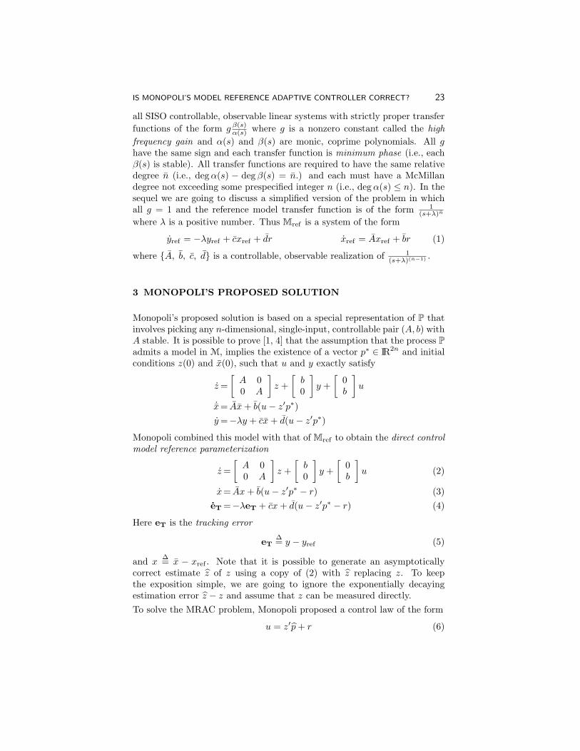
IS MONOPOLI’S MODEL REFERENCE ADAPTIVE CONTROLLER CORRECT? 23
all SISO controllable, observable linear systems with strictly proper transferfunctions of the form g β(s)
α(s) where g is a nonzero constant called the highfrequency gain and α(s) and β(s) are monic, coprime polynomials. All ghave the same sign and each transfer function is minimum phase (i.e., eachβ(s) is stable). All transfer functions are required to have the same relativedegree n (i.e., degα(s) − deg β(s) = n.) and each must have a McMillandegree not exceeding some prespecified integer n (i.e., degα(s) ≤ n). In thesequel we are going to discuss a simplified version of the problem in whichall g = 1 and the reference model transfer function is of the form 1
(s+λ)n
where λ is a positive number. Thus Mref is a system of the form
yref = −λyref + cxref + dr xref = Axref + br (1)
where A, b, c, d is a controllable, observable realization of 1(s+λ)(n−1) .
3 MONOPOLI’S PROPOSED SOLUTION
Monopoli’s proposed solution is based on a special representation of P thatinvolves picking any n-dimensional, single-input, controllable pair (A, b) withA stable. It is possible to prove [1, 4] that the assumption that the process Padmits a model in M, implies the existence of a vector p∗ ∈ IR2n and initialconditions z(0) and x(0), such that u and y exactly satisfy
z=[A 00 A
]z +
[b0
]y +
[0b
]u
˙x= Ax+ b(u− z′p∗)y=−λy + cx+ d(u− z′p∗)
Monopoli combined this model with that of Mref to obtain the direct controlmodel reference parameterization
z=[A 00 A
]z +
[b0
]y +
[0b
]u (2)
x= Ax+ b(u− z′p∗ − r) (3)eT =−λeT + cx+ d(u− z′p∗ − r) (4)
Here eT is the tracking error
eT∆= y − yref (5)
and x∆= x − xref . Note that it is possible to generate an asymptotically
correct estimate z of z using a copy of (2) with z replacing z. To keepthe exposition simple, we are going to ignore the exponentially decayingestimation error z − z and assume that z can be measured directly.To solve the MRAC problem, Monopoli proposed a control law of the form
u = z′p+ r (6)
24 PROBLEM 1.5
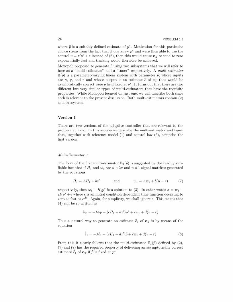
where p is a suitably defined estimate of p∗. Motivation for this particularchoice stems from the fact that if one knew p∗ and were thus able to use thecontrol u = z′p∗ + r instead of (6), then this would cause eT to tend to zeroexponentially fast and tracking would therefore be achieved.Monopoli proposed to generate p using two subsystems that we will refer tohere as a “multi-estimator” and a “tuner” respectively. A multi-estimatorE(p) is a parameter-varying linear system with parameter p, whose inputsare u, y, and r and whose output is an estimate e of eT that would beasymptotically correct were p held fixed at p∗. It turns out that there are twodifferent but very similar types of multi-estimators that have the requisiteproperties. While Monopoli focused on just one, we will describe both sinceeach is relevant to the present discussion. Both multi-estimators contain (2)as a subsystem.
Version 1
There are two versions of the adaptive controller that are relevant to theproblem at hand. In this section we describe the multi-estimator and tunerthat, together with reference model (1) and control law (6), comprise thefirst version.
Multi-Estimator 1
The form of the first multi-estimator E1(p) is suggested by the readily veri-fiable fact that if H1 and w1 are n× 2n and n× 1 signal matrices generatedby the equations
H1 = AH1 + bz′ and w1 = Aw1 + b(u− r) (7)
respectively, then w1 −H1p∗ is a solution to (3). In other words x = w1 −
H1p∗+ ε where ε is an initial condition dependent time function decaying to
zero as fast as eAt. Again, for simplicity, we shall ignore ε. This means that(4) can be re-written as
eT = −λeT − (cH1 + dz′)p∗ + cw1 + d(u− r)
Thus a natural way to generate an estimate e1 of eT is by means of theequation
˙e1 = −λe1 − (cH1 + dz′)p+ cw1 + d(u− r) (8)
From this it clearly follows that the multi-estimator E1(p) defined by (2),(7) and (8) has the required property of delivering an asymptotically correctestimate e1 of eT if p is fixed at p∗.

IS MONOPOLI’S MODEL REFERENCE ADAPTIVE CONTROLLER CORRECT? 25
Tuner 1
From (8) and the differential equation for eT directly above it, it can be seenthat the estimation error2
e1∆= e1 − eT (9)
satisfies the error equation
e1 = −λe1 + φ′1(p− p∗) (10)
where
φ′1 = −(cH1 + dz′) (11)
Prompted by this, Monopoli proposed to tune p1 using the pseudo-gradienttuner
˙p1 = −φ1e1 (12)
The motivation for considering this particular tuning law will become clearshortly, if it is not already.
What is known about Version 1?
The overall model reference adaptive controller proposed by Monopoli thusconsists of the reference model (1), the control law (6), the multi-estimator(2), (7), (8), the output estimation error (9) and the tuner (11), (12). Theopen problem is to prove that this controller either solves the model referenceadaptive control problem or that it does not.Much is known that is relevant to the problem. In the first place, note that(1), (2) together with (5) - (11) define a parameter varying linear systemΣ1(p) with input r, state (yref , xref , z,H1, w1, e1, e1) and output e1. Theconsequence of the assumption that every system in M is minimum phase isthat Σ1(p) is detectable through e1 for every fixed value of p [5]. Meanwhilethe form of (10) enables one to show by direct calculation, that the rate ofchange of the partial Lyapunov function V ∆= e21 + ||p−p∗||2 along a solutionto (12) and the equations defining Σ1(p), satisfies
V = −2λe21 ≤ 0 (13)
From this it is evident that V is a bounded monotone nonincreasing functionand consequently that e1 and p are bounded wherever they exist. Using andthe fact that Σ1(p) is a linear parameter-varying system, it can be concludedthat solutions exist globally and that e1 and p are bounded on [0,∞). Byintegrating (13) it can also be concluded that e1 has a finite L2[0,∞)-normand that ||e1||2 + ||p−p∗||2 tends to a finite limit as t→∞. Were it possibleto deduce from these properties that p tended to a limit p, then it wouldpossible to establish correctness of the overall adaptive controller using thedetectability of Σ1(p).
2Monopoli called e1 an augmented error.
26 PROBLEM 1.5
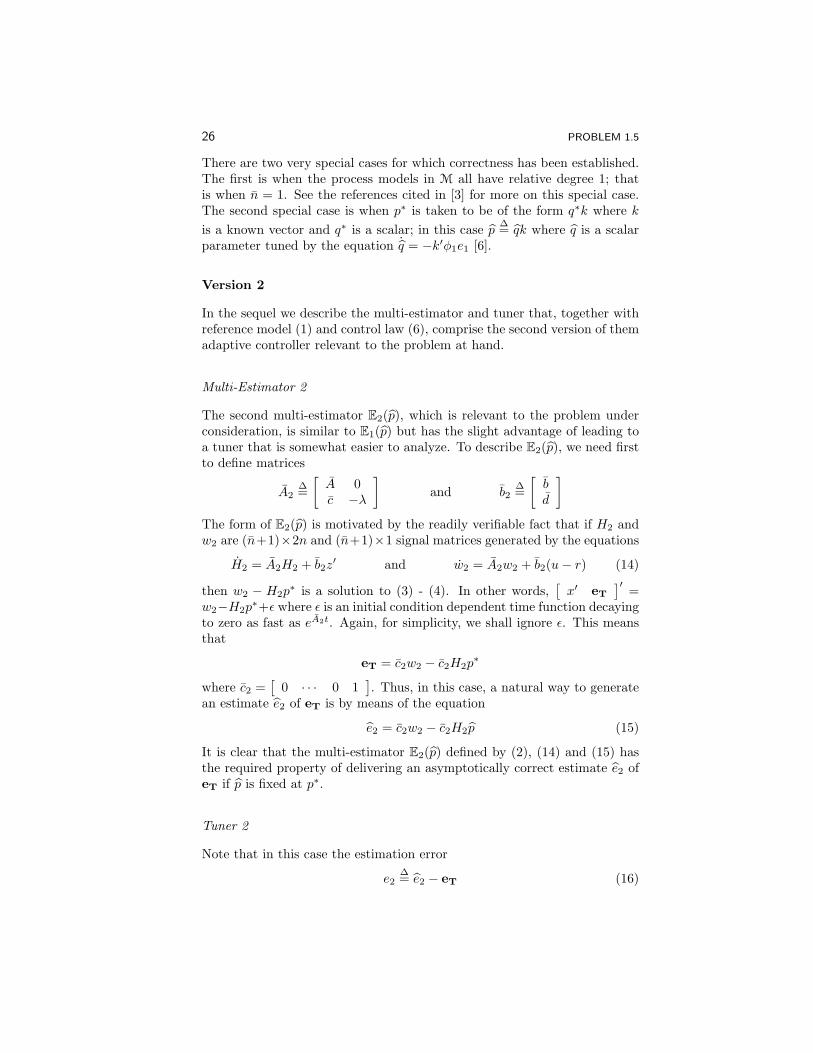
There are two very special cases for which correctness has been established.The first is when the process models in M all have relative degree 1; thatis when n = 1. See the references cited in [3] for more on this special case.The second special case is when p∗ is taken to be of the form q∗k where kis a known vector and q∗ is a scalar; in this case p ∆= qk where q is a scalarparameter tuned by the equation ˙q = −k′φ1e1 [6].
Version 2
In the sequel we describe the multi-estimator and tuner that, together withreference model (1) and control law (6), comprise the second version of themadaptive controller relevant to the problem at hand.
Multi-Estimator 2
The second multi-estimator E2(p), which is relevant to the problem underconsideration, is similar to E1(p) but has the slight advantage of leading toa tuner that is somewhat easier to analyze. To describe E2(p), we need firstto define matrices
A2∆=[A 0c −λ
]and b2
∆=[bd
]The form of E2(p) is motivated by the readily verifiable fact that if H2 andw2 are (n+1)×2n and (n+1)×1 signal matrices generated by the equations
H2 = A2H2 + b2z′ and w2 = A2w2 + b2(u− r) (14)
then w2 − H2p∗ is a solution to (3) - (4). In other words,
[x′ eT
]′ =w2−H2p
∗+ε where ε is an initial condition dependent time function decayingto zero as fast as eA2t. Again, for simplicity, we shall ignore ε. This meansthat
eT = c2w2 − c2H2p∗
where c2 =[
0 · · · 0 1]. Thus, in this case, a natural way to generate
an estimate e2 of eT is by means of the equation
e2 = c2w2 − c2H2p (15)
It is clear that the multi-estimator E2(p) defined by (2), (14) and (15) hasthe required property of delivering an asymptotically correct estimate e2 ofeT if p is fixed at p∗.
Tuner 2
Note that in this case the estimation error
e2∆= e2 − eT (16)
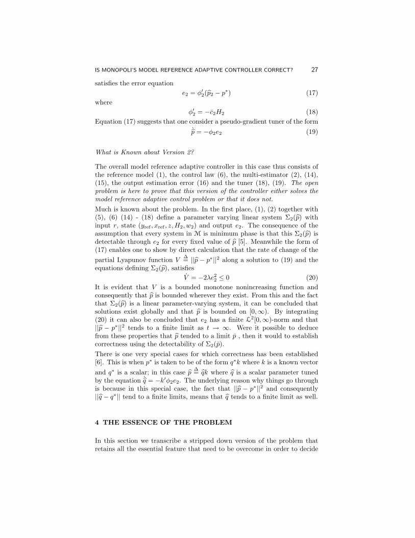
IS MONOPOLI’S MODEL REFERENCE ADAPTIVE CONTROLLER CORRECT? 27
satisfies the error equatione2 = φ′2(p2 − p∗) (17)
whereφ′2 = −c2H2 (18)
Equation (17) suggests that one consider a pseudo-gradient tuner of the form˙p = −φ2e2 (19)
What is Known about Version 2?
The overall model reference adaptive controller in this case thus consists ofthe reference model (1), the control law (6), the multi-estimator (2), (14),(15), the output estimation error (16) and the tuner (18), (19). The openproblem is here to prove that this version of the controller either solves themodel reference adaptive control problem or that it does not.Much is known about the problem. In the first place, (1), (2) together with(5), (6) (14) - (18) define a parameter varying linear system Σ2(p) withinput r, state (yref , xref , z,H2, w2) and output e2. The consequence of theassumption that every system in M is minimum phase is that this Σ2(p) isdetectable through e2 for every fixed value of p [5]. Meanwhile the form of(17) enables one to show by direct calculation that the rate of change of thepartial Lyapunov function V
∆= ||p − p∗||2 along a solution to (19) and theequations defining Σ2(p), satisfies
V = −2λe22 ≤ 0 (20)It is evident that V is a bounded monotone nonincreasing function andconsequently that p is bounded wherever they exist. From this and the factthat Σ2(p) is a linear parameter-varying system, it can be concluded thatsolutions exist globally and that p is bounded on [0,∞). By integrating(20) it can also be concluded that e2 has a finite L2[0,∞)-norm and that||p − p∗||2 tends to a finite limit as t → ∞. Were it possible to deducefrom these properties that p tended to a limit p , then it would to establishcorrectness using the detectability of Σ2(p).There is one very special cases for which correctness has been established[6]. This is when p∗ is taken to be of the form q∗k where k is a known vectorand q∗ is a scalar; in this case p ∆= qk where q is a scalar parameter tunedby the equation ˙q = −k′φ2e2. The underlying reason why things go throughis because in this special case, the fact that ||p − p∗||2 and consequently||q − q∗|| tend to a finite limits, means that q tends to a finite limit as well.
4 THE ESSENCE OF THE PROBLEM
In this section we transcribe a stripped down version of the problem thatretains all the essential feature that need to be overcome in order to decide
28 PROBLEM 1.5
whether or not Monopoli’s controller is correct. We do this only for version2 of the problem and only for the case when r = 0 and n = 1. Thus, inthis case, we can take A2 = −λ and b2 = 1. Assuming the reference modelis initialized at 0, dropping the subscript 2 throughout, and writing φ′ for−H, the system to be analyzed reduces to
z=[A 00 A
]z +
[b0
](w + φ′p∗) +
[0b
]p′z (21)
φ=−λφ− z (22)w=−λw + p′z (23)e=φ′(p− p∗) (24)˙p=−φe (25)
To recap, p∗ is unknown and constant but is such that the linear parameter-varying system Σ(p) defined by (21) to (24) is detectable through e foreach fixed value of p. Solutions to the system (21) - (25) exist globally.The parameter vector p and integral square of e are bounded on [0,∞) and||p− p∗|| tends to a finite limit as t→∞. The open problem here is to showfor every initialization of (21)-(25), that the state of Σ(p) tends to 0 or thatit does not.
BIBLIOGRAPHY
[1] R. V. Monopoli, “Model reference adaptive control with an augmentederror,” IEEE Transactions on Automatic Control, pp. 474–484, October1974.
[2] A. Feuer, B. R. Barmish, and A. S. Morse, “An unstable system as-sociated with model reference adaptive control,” IEEE Transactions onAutomatic Control, 23:499–500, 1978.
[3] A. S. Morse, “Overcoming the obstacle of high relative degree,” EuropeanJournal of Control, 2(1):29–35, 1996.
[4] K. J. Astrom and B. Wittenmark, “On self-tuning regulators,” Automat-ica, 9:185–199, 1973.
[5] A. S. Morse, “Towards a unified theory of parameter adaptive control -Part 2: Certainty equivalence and implicit tuning,” IEEE Transactionson Automatic Control, 37(1):15–29, January 1992.
[6] A. Feuer, Adaptive Control of Single Input Single Output Linear Systems,Ph.D. thesis, Yale University, 1978.
Problem 1.6
Model reduction of delay systems
Jonathan R. PartingtonSchool of MathematicsUniversity of LeedsLeeds, LS2 [email protected]
1 DESCRIPTION OF THE PROBLEM
Our concern here is with stable single input single output delay systems,and we shall restrict to the case when the system has a transfer functionof the form G(s) = e−sTR(s), with T > 0 and R rational, stable, andstrictly proper, thus bounded and analytic on the right half plane C+. It isa fundamental problem in robust control design to approximate such systemsby finite-dimensional systems. Thus, for a fixed natural number n, we wishto find a rational approximant Gn(s) of degree at most n in order to makesmall the approximation error ‖G−Gn‖, where ‖ . ‖ denotes an appropriatenorm. See [9] for some recent work on this subject.Commonly used norms on a linear time-invariant system with impulse re-sponse g ∈ L1(0,∞) and transfer function G ∈ H∞(C+) are the H∞
norm ‖G‖∞ = supRe s>0 |G(s)|, the Lp norms ‖g‖p =(∫∞
0|g(t)|p dt
)1/p(1 ≤ p < ∞), and the Hankel norm ‖Γ‖, where Γ : L2(0,∞) → L2(0,∞) isthe Hankel operator defined by
(Γu)(t) =∫ ∞
0
g(t+ τ)u(τ) dτ.
These norms are related by
‖Γ‖ ≤ ‖G‖∞ ≤ ‖g‖1 ≤ 2n‖Γ‖,where the last inequality holds for systems of degree at most n.
Two particular approximation techniques for finite-dimensional systems arewell-established in the literature [14], and they can also be used for someinfinite-dimensional systems [5]:
30 PROBLEM 1.6
• Truncated balanced realizations, or, equivalently, output normal real-izations [11, 13, 5];
• Optimal Hankel-norm approximants [1, 4, 5].
As we explain in the next section, these techniques are known to produceH∞-convergent sequences of approximants for many classes of delay systems(systems of nuclear type). We are thus led to pose the following question:Do the sequences of reduced order models produced by truncated balancedrealizations and optimal Hankel-norm approximations converge for all stabledelay systems?
2 MOTIVATION AND HISTORY OF THE PROBLEM
Balanced realizations were introduced in [11], and many properties of trun-cations of such realizations were given in [13]. An H∞ error bound for thereduced-order system produced by truncating a balanced realization wasgiven for finite-dimensional systems in [3, 4], and extended to infinite-di-mensional systems in [5]. This commonly used bound is expressed in termsof the sequence (σk)∞k=1 of singular values of the Hankel operator Γ corre-sponding to the original system G; in our case Γ is compact, and so σk → 0.Provided that g ∈ L1∩L2 and Γ is nuclear (i.e.,
∑∞k=1 σk <∞) with distinct
singular values, then the inequality
‖G−Gbn‖∞ ≤ 2(σn+1 + σn+2 + . . .)
holds for the degree-n balanced truncation Gbn of G. The elementary lowerbound ‖G−Gn‖ ≥ σn+1 holds for any degree-n approximation to G.
Another numerically convenient approximation method is the optimal Han-kel-norm technique [1, 4, 5], which involves finding a best rank-n Hankelapproximation ΓHn to Γ, in the Hankel norm, so that ‖Γ− ΓHn ‖ = σn+1. Inthis case the bound
‖G−GHn −D0‖∞ ≤ σn+1 + σn+2 + . . .
is available for the corresponding transfer function GHn with a suitable con-stant D0. Again, we require the nuclearity of Γ for this to be meaningful.
3 AVAILABLE RESULTS
In the case of a delay system G(s) = e−sTR(s) as specified above, it is known
that the Hankel singular values σk are asymptotic to A(Tπk
)r, where r is
MODEL REDUCTION OF DELAY SYSTEMS 31
the relative degree of R and |srR(s)| tends to the finite nonzero limit A as|s| → ∞. Hence Γ is nuclear if and only if the relative degree of R is at least2. (Equivalently, if and only if g is continuous.) We refer to [6, 7] for theseand more precise results.
Even for a very simple non-nuclear system such as G(s) = e−sT
s+ 1, for whichkσk → T/π, no theoretical upper bound is known for the H∞ errors inthe rational approximants produced by truncated balanced realizations andoptimal Hankel-norm approximation, although numerical evidence suggeststhat they should still tend to zero.
A related question is to find the best error bounds in L1 approximation ofa delay system. For example, a smoothing technique gives an L1 approx-imation error O
(lnnn
)for systems of relative degree r = 1 (see [8]), and
it is possible that the optimal Hankel norm might yield a similar rate ofconvergence. (A lower bound of C/n for some constant C > 0 follows easilyfrom the above discussion.)
One approach that may be useful in these analyses is to exploit Bonsall’stheorem that a Hankel integral operator Γ is bounded if and only if it isuniformly bounded on the set of all normalized L2 functions whose Laplacetransforms are rational of degree one [2, 12]. An explicit constant in Bon-sall’s theorem is not known, and would be of great interest in its own right.
Another approach which may be relevant is that of Megretski [10], whointroduces maximal real part norms. Their interest stems from the inequality‖G‖∞ ≥ ‖ReG‖∞ ≥ ‖Γ‖/2.
BIBLIOGRAPHY
[1] V. M. Adamjan, D. Z. Arov, and M. G. Kreın, “Analytic properties ofSchmidt pairs for a Hankel operator and the generalized Schur–Takagiproblem,” Math. USSR Sbornik, 15:31–73, 1971.
[2] F. F. Bonsall, “Boundedness of Hankel matrices”, J. London Math. Soc.(2), 29(2):289–300, 1984.
[3] D. Enns, Model Reduction for Control System Design, Ph.D. disserta-tion, Stanford University, 1984.
[4] K. Glover, “All optimal Hankel-norm approximations of linear mul-tivariable systems and their L∞-error bounds, Internat. J. Control,39(6):1115–1193, 1984.
32 PROBLEM 1.6
[5] K. Glover, R. F. Curtain, and J. R. Partington, “Realisation and ap-proximation of linear infinite-dimensional systems with error bounds,”SIAM J. Control Optim., 26(4):863–898, 1988.
[6] K. Glover, J. Lam, and J. R. Partington, “Rational approximation of aclass of infinite-dimensional systems. I. Singular values of Hankel oper-ators,” Math. Control Signals Systems, 3(4):325–344, 1990.
[7] K. Glover, J. Lam, and J. R. Partington,“Rational approximation of aclass of infinite-dimensional systems. II. Optimal convergence rates ofL∞ approximants,” Math. Control Signals Systems, 4(3):233–246, 1991.
[8] K. Glover and J. R. Partington, “Bounds on the achievable accuracy inmodel reduction,” In: Modelling, Robustness and Sensitivity Reductionin Control Systems (Groningen, 1986), pp. 95–118. Springer, Berlin,1987.
[9] P. M. Makila and J. R. Partington, “Shift operator induced approxi-mations of delay systems,” SIAM J. Control Optim., 37(6):1897–1912,1999.
[10] A. Megretski, “Model order reduction using maximal real part norms,”Presented at CDC 2000, Sydney, 2000.http://web.mit.edu/ameg/www/images/lund.ps.
[11] B. C. Moore, “Principal component analysis in linear systems: control-lability, observability, and model reduction,” IEEE Trans. Automat.Control, 26(1):17–32, 1981.
[12] J. R. Partington and G. Weiss, “Admissible observation operators forthe right-shift semigroup,” Math. Control Signals Systems, 13(3):179–192, 2000.
[13] L. Pernebo and L. M. Silverman, “Model reduction via balanced statespace representations,” IEEE Trans. Automat. Control, 27(2):382–387,1982.
[14] K. Zhou, J. C. Doyle, and K. Glover, Robust and Optimal Control,Upper Saddle River, NJ: Prentice Hall1996.
Problem 1.7
Schur extremal problems
Lev SakhnovichCourant Institute of Mathematical ScienceNew York, NY [email protected]
1 DESCRIPTION OF THE PROBLEM
In this paper we consider the well-known Schur problem the solution of whichsatisfy in addition the extremal condition
w?(z)w(z) ≤ ρ2min, |z| < 1, (1)
where w(z) and ρmin are m ×m matrices and ρmin > 0. Here the matrixρmin is defined by a certain minimal-rank condition (see Definition 1). Weremark that the extremal Schur problem is a particular case. The generalcase is considered in book [1] and paper [2]. Our approach to the extremalproblems does not coincide with the superoptimal approach [3],[4]. In paper[2] we compare our approach to the extremal problems with the superoptimalapproach. Interpolation has found great applications in control theory [5],[6].
Schur Extremal Problem: The m×m matrices a0, a1, ..., an are given.Describe the set of m×m matrix functions w(z) holomorphic in the circle|z| < 1 and satisfying the relation
w(z) = a0 + a1z + ...+ anzn + ... (2)
and inequality (1.1).A necessary condition of the solvability of the Schur extremal problem is theinequality
R2min − S ≥ 0, (3)
where the (n + 1)m×(n + 1)m matrices S and Rmin are defined by therelations
S = CnC?n, Rmin = diag[ρmin, ρmin, ..., ρmin], (4)

34 PROBLEM 1.7
Cn =
a0 0 ... 0a1 a0 ... 0... ... ... ...an an−1 ... a0
. (5)
Definition 1: We shall call the matrix ρ = ρmin > 0 minimal if the followingtwo requirements are fulfilled:1. The inequality
R2min − S ≥ 0 (6)
holds.2. If the m×m matrix ρ > 0 is such that
R2 − S ≥ 0, (7)then
rank(R2min − S) ≤ rank(R2 − S), (8)
where R = diag[ρ, ρ, ..., ρ].Remark 1: The existence of ρmin follows directly from definition 1.Question 1: Is ρmin unique?Remark 2: If m = 1 then ρmin is unique and ρ2
min = λmax, where λmax isthe largest eigenvalue of the matrix S.Remark 3: Under some assumptions the uniqueness of ρmin is proved inthe case m > 1, n = 1 (see [2],[7]).
If ρmin is known then the corresponding wmin(ξ) is a rational matrix func-tion. This generalizes the well-known fact for the scalar case (see [7]).Question 2: How to find ρmin?In order to describe some results in this direction we write the matrixS = CnC
?n in the following block form(
S11 S12
S21 S22
), (9)
where S22 is an m×m matrix.Proposition 1: [1] If ρ = q > 0 satisfies inequality (1.7) and the relation
q2 = S22 + S?12(Q2 − S11)−1S12, (10)
where Q = diag[q, q, ..., q], then ρmin = q.We shall apply the method of successive approximation when studying equa-tion (1.10). We put q20 = S22, q2k+1 = S22 +S?12(Q
2k − S11)−1S12, where k≥0,
Qk = diag[qk, qk, ..., qk]. We suppose thatQ2
0 − S11 > 0. (11)Theorem 1: [1] The sequence q20 , q
22 , q
24 , ... monotonically increases and has
the limit m1. The sequence q21 , q23 , q
25 , ... monotonically decreases and has the
limit m2. The inequality m1≤m2 holds. If m1 = m2 then ρ2min = q2.
Question 3: Suppose relation (1.11) holds. Is there a case when m1 6=m2?The answer is “no” if n = 1 (see [2],[8]).Remark 4: In book [1] we give an example in which ρmin is constructed inexplicit form.
SCHUR EXTREMAL PROBLEMS 35
BIBLIOGRAPHY
[1] Lev Sakhnovich. Interpolation Theory and Applications, KluwerAcad.Publ. (1997).
[2] J. Helton and L. Sakhnovich, Extremal Problems of Interpolation Theory(forthcoming).
[3] N. J. Young, “The Nevanlinna-Pick Problem for matrix-valued func-tions,” J. Operator Theory, 15, pp. 239–265, (1986).
[4] V. V. Peller and N. J. Young, “Superoptimal analytic approximationsof matrix functions,” Journal of Functional Analysis, 120, pp. 300–343,(1994).
[5] M. Green and D. Limebeer, Linear Robust Control, Prentice-Hall, (1995).
[6] “Lecture Notes in Control and Information,” Sciences, Springer Verlag,135 (1989).
[7] N. I. Akhiezer, “On a Minimum in Function Theory,” Operator Theory,Adv. and Appl. 95, pp. 19–35, (1997).
[8] A. Ferrante and B. C. Levy, “Hermitian Solutions of the Equations X =Q+NX−1N?,” Linear Algebra and Applications 247, pp. 359-373, (1996).

Problem 1.8
The elusive iff test for time-controllability of
behaviours
Amol SasaneFaculty of Mathematical SciencesUniversity of Twente7500 AE, EnschedeThe [email protected]
1 DESCRIPTION OF THE PROBLEM
Problem: Let R ∈ C[η1, . . . , ηm, ξ]g×w and let B be the behavior given bythe kernel representation corresponding to R. Find an algebraic test on Rcharacterizing the time-controllability of B.
In the above, we assume B to comprise of only smooth trajectories, that is,
B =w ∈ C∞
(Rm+1,Cw
)| DRw = 0
,
where DR : C∞(Rm+1,Cw
)→ C∞
(Rm+1,Cg
)is the differential map that acts
as follows: if R =[rij]g×w
, then
DR
w1
...ww
=
∑w
k=1 r1k
(∂∂x1
, . . . , ∂∂xm
, ∂∂t
)wk
...∑wk=1 rgk
(∂∂x1
, . . . , ∂∂xm
, ∂∂t
)wk
.Time-controllability is a property of the behavior, defined as follows. Thebehavior B is said to be time-controllable if for any w1 and w2 in B, thereexists a w ∈ B and a τ ≥ 0 such that
w(•, t) =w1(•, t) for all t ≤ 0w2(•, t− τ) for all t ≥ τ
.
THE ELUSIVE IFF TEST FOR TIME-CONTROLLABILITY 37
2 MOTIVATION AND HISTORY OF THE PROBLEM
The behavioral theory for systems described by a set of linear constant coef-ficient partial differential equations has been a challenging and fruitful areaof research for quite some time (see, for instance, Pillai and Shankar [5],Oberst [3] and Wood et al. [4]). An excellent elementary introduction tothe behavioral theory in the 1−D case (corresponding to systems describedby a set of linear constant coefficient ordinary differential equations) can befound in Polderman and Willems [6].In [5], [3] and [4], the behaviours arising from systems of partial differentialequations are studied in a general setting in which the time-axis does notplay a distinguished role in the formulation of the definitions pertinent tocontrol theory. Since in the study of systems with “dynamics,” it is useful togive special importance to time in defining system theoretic concepts, recentattempts have been made in this direction (see, for example, Cotroneo andSasane [2], Sasane et al. [7], and Camlıbel and Sasane [1]). The formulationof definitions with special emphasis on the time-axis is straightforward, sincethey can be seen quite easily as extensions of the pertinent definitions in the1−D case. However, the algebraic characterization of the properties of thebehavior, such as time-controllability, turn out to be quite involved.Although the traditional treatment of distributed parameter systems (inwhich one views them as an ordinary differential equation with an infinite-dimensional Hilbert space as the state-space) is quite successful, the studyof the present problem will have its advantages, since it would give a testthat is algebraic in nature (and hence computationally easy) for a propertyof the sets of trajectories, namely time-controllability. Another motivationfor considering this problem is that the problem of patching up of solutionsof partial differential equations is also an interesting question from a purelymathematical point of view.
3 AVAILABLE RESULTS
In the 1−D case, it is well-known (see, for example, theorem 5.2.5 on page154 of [6]) that time-controllability is equivalent with the following condition:There exists a r0 ∈ N ∪ 0 such that for all λ ∈ C, rank(R(λ)) = r0. Thiscondition is in turn equivalent with the torsion freeness of the C[ξ]-moduleC[ξ]w/C[ξ]gR.Let us consider the following statements
A1. The C(η1, . . . , ηm)[ξ]-module C(η1, . . . , ηm)[ξ]w/C(η1, . . . , ηm)[ξ]gR is tor-sion free.
A2. There exists a χ ∈ C[η1, . . . , ηm, ξ]w \C(η1, . . . , ηm)[ξ]gR and there existsa nonzero p ∈ C[η1, . . . , ηm, ξ] such that p · χ ∈ C(η1, . . . , ηm)[ξ]gR, and
38 PROBLEM 1.8
deg(p) = deg((p)), where denotes the homomorphismp(ξ, η1, . . . , ηm) 7→ p(ξ, 0, . . . , 0) : C[ξ, η1, . . . , ηm] → C[ξ].
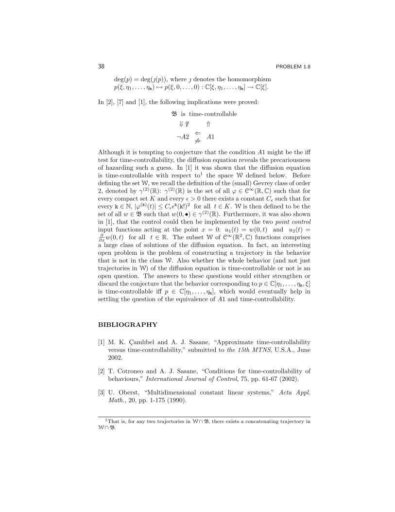
In [2], [7] and [1], the following implications were proved:
B is time-controllable⇓ 6⇑ ⇑
¬A2⇐6⇒ A1
Although it is tempting to conjecture that the condition A1 might be the ifftest for time-controllability, the diffusion equation reveals the precariousnessof hazarding such a guess. In [1] it was shown that the diffusion equationis time-controllable with respect to1 the space W defined below. Beforedefining the set W, we recall the definition of the (small) Gevrey class of order2, denoted by γ(2)(R): γ(2)(R) is the set of all ϕ ∈ C∞(R,C) such that forevery compact set K and every ε > 0 there exists a constant Cε such that forevery k ∈ N, |ϕ(k)(t)| ≤ Cεε
k(k!)2 for all t ∈ K. W is then defined to be theset of all w ∈ B such that w(0, •) ∈ γ(2)(R). Furthermore, it was also shownin [1], that the control could then be implemented by the two point controlinput functions acting at the point x = 0: u1(t) = w(0, t) and u2(t) =∂∂xw(0, t) for all t ∈ R. The subset W of C∞(R2,C) functions comprisesa large class of solutions of the diffusion equation. In fact, an interestingopen problem is the problem of constructing a trajectory in the behaviorthat is not in the class W. Also whether the whole behavior (and not justtrajectories in W) of the diffusion equation is time-controllable or not is anopen question. The answers to these questions would either strengthen ordiscard the conjecture that the behavior corresponding to p ∈ C[η1, . . . , ηm, ξ]is time-controllable iff p ∈ C[η1, . . . , ηm], which would eventually help insettling the question of the equivalence of A1 and time-controllability.
BIBLIOGRAPHY
[1] M. K. Camlıbel and A. J. Sasane, “Approximate time-controllabilityversus time-controllability,” submitted to the 15th MTNS, U.S.A., June2002.
[2] T. Cotroneo and A. J. Sasane, “Conditions for time-controllability ofbehaviours,” International Journal of Control, 75, pp. 61-67 (2002).
[3] U. Oberst, “Multidimensional constant linear systems,” Acta Appl.Math., 20, pp. 1-175 (1990).
1That is, for any two trajectories in W ∩B, there exists a concatenating trajectory inW ∩B.
THE ELUSIVE IFF TEST FOR TIME-CONTROLLABILITY 39
[4] D. H. Owens, E. Rogers and J. Wood, “Controllable and autonomousn−D linear systems,” Multidimensional Systems and Signal Processing,10, pp. 33-69 (1999).
[5] H. K. Pillai and S. Shankar, “A Behavioural Approach to the Control ofDistributed Systems,” SIAM Journal on Control and Optimization, 37,pp. 388-408 (1998).
[6] J. W. Polderman and J. C. Willems, Introduction to Mathematical Sys-tems Theory, Springer-Verlag, 1998.
[7] A. J. Sasane, E. G. F. Thomas and J. C. Willems, “Time-autonomyversus time-controllability,” accepted for publication in The Systems andControl Letters, 2001.
Problem 1.9
A Farkas lemma for behavioral inequalities
A. A. (Tonny) ten DamInformation, Communication and Technology DivisionNational Aerospace Laboratory NLRP.O. Box 90502 , 1006 BM AmsterdamThe [email protected]
J.W. (Hans) NieuwenhuisFaculty of EconomicsUniversity of GroningenPostbus 800, 9700 AV GroningenThe [email protected]
1 DESCRIPTION OF THE PROBLEM
Within the systems and control community there has always been an interestin minimality issues. In this chapter we conjecture a Farkas Lemma forbehavioral inequalities that, when true, will allow to study minimality andelimation issues for behavioral systems described by inequalities.Let Rn×m[s, s−1] denote the (n × m) polynomial matrices with real co-efficients and positive and negative powers in the indeterminate s. LetRn×m+ [s, s−1] denote the set of matrices in Rn×m[s, s−1] with non-negativecoefficients only. In this chapter we consider discrete-time systems withtime-axis Z. Let σ denote the (backward) shift operator, and let R(σ, σ−1)denote polynomial operators in the shift.Of interest is the relation between two polynomial matrices R(s, s−1) andR′(s, s−1) when they satisfy
R(σ, σ−1)w ≥ 0 ⇒ R′(σ, σ−1)w ≥ 0. (1)
Based on the static case, one may expect that such a relation should be theextension of Farkas’s lemma to the behavioral case. This leads to the raisond’tre of this chapter.
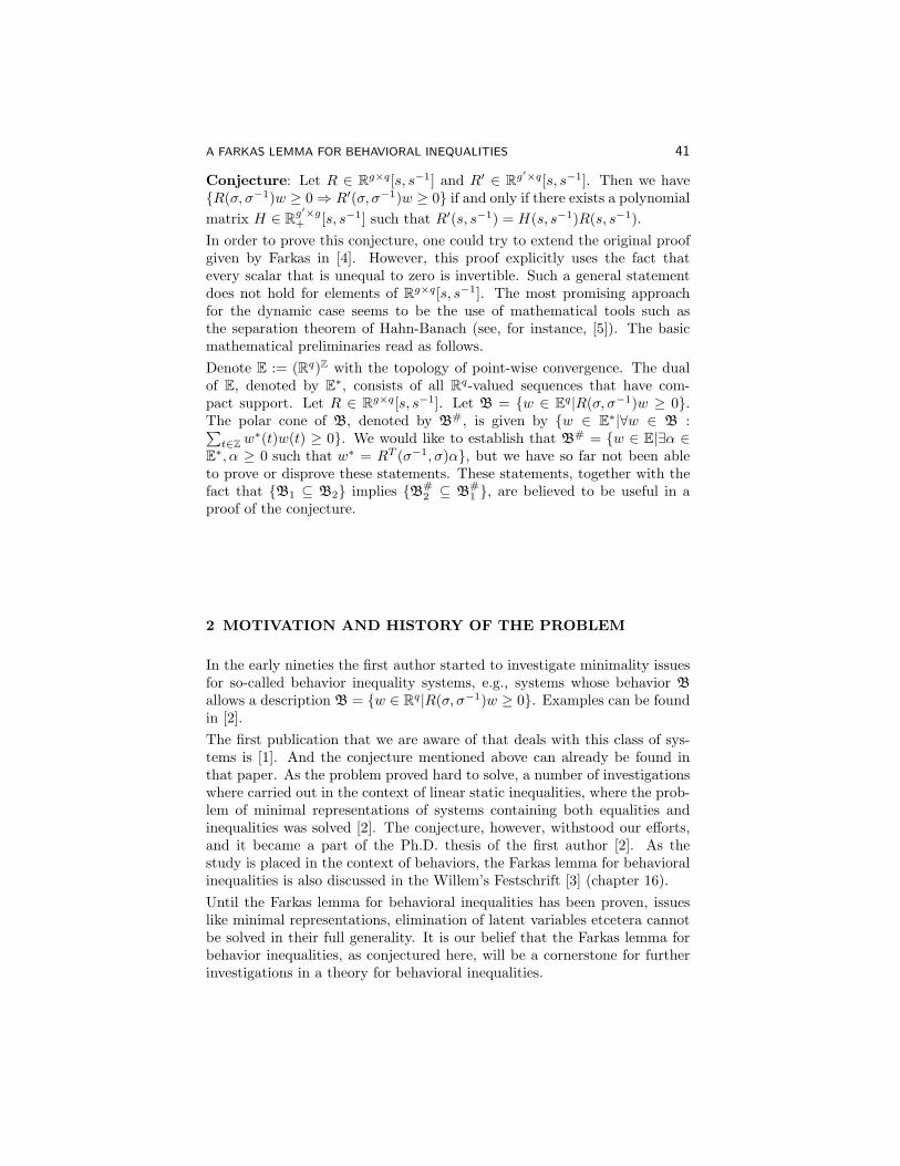
A FARKAS LEMMA FOR BEHAVIORAL INEQUALITIES 41
Conjecture: Let R ∈ Rg×q[s, s−1] and R′ ∈ Rg′×q[s, s−1]. Then we haveR(σ, σ−1)w ≥ 0 ⇒ R′(σ, σ−1)w ≥ 0 if and only if there exists a polynomialmatrix H ∈ Rg
′×g+ [s, s−1] such that R′(s, s−1) = H(s, s−1)R(s, s−1).
In order to prove this conjecture, one could try to extend the original proofgiven by Farkas in [4]. However, this proof explicitly uses the fact thatevery scalar that is unequal to zero is invertible. Such a general statementdoes not hold for elements of Rg×q[s, s−1]. The most promising approachfor the dynamic case seems to be the use of mathematical tools such asthe separation theorem of Hahn-Banach (see, for instance, [5]). The basicmathematical preliminaries read as follows.Denote E := (Rq)Z with the topology of point-wise convergence. The dualof E, denoted by E∗, consists of all Rq-valued sequences that have com-pact support. Let R ∈ Rg×q[s, s−1]. Let B = w ∈ Eq|R(σ, σ−1)w ≥ 0.The polar cone of B, denoted by B#, is given by w ∈ E∗|∀w ∈ B :∑t∈Z w
∗(t)w(t) ≥ 0. We would like to establish that B# = w ∈ E|∃α ∈E∗, α ≥ 0 such that w∗ = RT (σ−1, σ)α, but we have so far not been ableto prove or disprove these statements. These statements, together with thefact that B1 ⊆ B2 implies B#
2 ⊆ B#1 , are believed to be useful in a
proof of the conjecture.
2 MOTIVATION AND HISTORY OF THE PROBLEM
In the early nineties the first author started to investigate minimality issuesfor so-called behavior inequality systems, e.g., systems whose behavior Ballows a description B = w ∈ Rq|R(σ, σ−1)w ≥ 0. Examples can be foundin [2].The first publication that we are aware of that deals with this class of sys-tems is [1]. And the conjecture mentioned above can already be found inthat paper. As the problem proved hard to solve, a number of investigationswhere carried out in the context of linear static inequalities, where the prob-lem of minimal representations of systems containing both equalities andinequalities was solved [2]. The conjecture, however, withstood our efforts,and it became a part of the Ph.D. thesis of the first author [2]. As thestudy is placed in the context of behaviors, the Farkas lemma for behavioralinequalities is also discussed in the Willem’s Festschrift [3] (chapter 16).Until the Farkas lemma for behavioral inequalities has been proven, issueslike minimal representations, elimination of latent variables etcetera cannotbe solved in their full generality. It is our belief that the Farkas lemma forbehavior inequalities, as conjectured here, will be a cornerstone for furtherinvestigations in a theory for behavioral inequalities.
42 PROBLEM 1.9
3 AVAILABLE RESULTS
For the static case, the conjecture is nothing else than the famous Farkaslemma for linear inqualities. For the dynamic case, the conjecture holds truefor a special case.Proposition: Let R ∈ Rg×q[s, s−1] be a full-row rank polynomial matrix.Let R′ ∈ Rg′×q[s, s−1]. Then: R(σ, σ−1)w ≥ 0 ⇒ R′(σ, σ−1)w ≥ 0 if andonly if there exists a unique polynomial matrix H ∈ Rg
′×g+ [s, s−1] such that
R′(s, s−1) = H(s, s−1)R(s, s−1).The proof of this proposition can be found in [2] (proposition 4.5.12).
4 A RELATED CONJECTURE
It is of interest to present a related conjecture, whose resolution is closelylinked to the Farkas lemma for behavioral inequalities.Recall from [6] that a matrix U ∈ Rg×g[s, s−1] is said to be unimodular if ithas an inverse U−1 ∈ Rg×g[s, s−1]. We will call a matrix H ∈ Rg×g+ [s, s−1]posimodular if it is unimodular and H−1 ∈ Rg×g+ [s, s−1]. Omitting theformal definitions, we will call a representation minimal if the number ofequations used to describe the behavior is minimal.Conjecture: Let w ∈ (Rq)Z|R1(σ, σ−1)w = 0 and R2(σ, σ−1)w ≥ 0 andw ∈ (Rq)Z|R′1(σ, σ−1)w = 0 and R′2(σ, σ
−1)w ≥ 0 both be two minimalrepresentations. They represent the same behavior if and only if there arepolynomial matrices U(s, s−1), H(s, s−1) and S(s, s−1) such that[
R′1(s, s−1)
R′2(s, s−1)
]=[U(s, s−1) 0S(s, s−1) H(s, s−1)
] [R1(s, s−1)R2(s, s−1)
](2)
with U unimodular, H posimodular and no conditions on S.We remark that this conjecture holds true for static inequalities and for thatcase is given as proposition 3.4.5 in [2].
BIBLIOGRAPHY
[1] A. A. ten Dam, “Representations of dynamical systems described bybehavioural inequalities,” In: Proceedings European Control ConferenceECC’93, vol. 3, pp. 1780-1783, June 28-July 1, Groningen, The Nether-lands, 1993.
[2] A. A. ten Dam, Unilaterally Constrained Dynamical Systems, Ph.D.Dissertation, University Groningen, The Netherlands, 1997. URL:http://www.ub.rug.nl/eldoc/dis/science/a.a.ten.dam/
A FARKAS LEMMA FOR BEHAVIORAL INEQUALITIES 43
[3] A. A. ten Dam and J. W. Nieuwenhuis, “On behavioural inequalities,” In:The Mathematics from Systems and Control: From Intelligent Controlto Behavioral Systems, Groningen, 1999, pp. 165-176.
[4] J. Farkas, “Die algebraische Grundlage der Anwendungen des Mechanis-chen Princips von Fourier,” Mathematische und naturwissenschaftlicheBerichte aus Ungarn, 16, pp. 154-157, 1899. (Translation of: Gy. Farkas,“A Fourier-fele mechanikai elv alkalmazasanak algebrai alapja,” Mathe-matikai es Termeszettudomanyi Ertesıto, 16, pp. 361-364, 1898.)
[5] W. Rudin, Functional Analysis, Tata McGraw-Hill Publishing CompanyLtd., 1973.
[6] J.C. Willems, “Paradigms and puzzles in the theory of dynamical sys-tems,” IEEE Transactions on Automatic Control, vol. 36, no. 3, pp.259-294, 1991.
Problem 1.10
Regular feedback implementability of linear
differential behaviors
H. L. TrentelmanMathematics InstituteUniversity of GroningenP.O. Box 800, 9700 AV GroningenThe [email protected]
1 INTRODUCTION
In this short paper, we want to discuss an open problem that appears in thecontext of interconnection of systems in a behavioral framework. Given asystem behavior, playing the role of plant to be controlled, the problem is tocharacterize all system behaviors that can be achieved by interconnecting theplant behavior with a controller behavior, where the interconnection shouldbe a regular feedback interconnection.More specifically, we will deal with linear time-invariant differential systems,i.e., dynamical systems Σ given as a triple R,Rw,B, where R is the time-axis, and where B, called the behavior of the system Σ, is equal to the set ofall solutions w : R → Rw of a set of higher order, linear, constant coefficient,differential equations. More precisely,
B = w ∈ C∞(R,Rw | R(d
dt)w = 0,
for some polynomial matrix R ∈ R•×w[ξ]. The set of all such systems Σ isdenoted by Lw. Often, we simply refer to a system by talking about its be-havior, and we write B ∈ Lw instead of Σ ∈ Lw. Behaviors B ∈ Lw can hencebe described by differential equations of the form R( ddt )w = 0, typically withthe number of rows of R strictly less than its number of columns. Mathemat-ically, R( ddt )w = 0 is then an under-determined system of equations. Thisresults in the fact that some of the components of w = (w1, w2, . . . , ww) areunconstrained. This number of unconstrained components is an integer “in-variant” associated with B, and is called the input cardinality of B, denotedby m(B), its number of free, “input,” variables. The remaining number of
REGULAR FEEDBACK IMPLEMENTABILITY 45
variables, w − m(B), is called the output cardinality of B and is denoted byp(B). Finally, a third integer invariant associated with a system behaviorB ∈ Lw is its McMillan degree. It can be shown that (modulo permutationof the components of the external variable w) any B ∈ Lw can be representedby a state space representation of the form d
dtx = Ax + Bu, y = Cx +Du,w = (u, y). Here, A,B,C, and D are constant matrices with real compo-nents. The minimal number of components of the state variable x neededin such an input/state/output representation of B is called the McMillandegree of B, and is denoted by n(B).Suppose now Σ1 = R,Rw1×Rw2 ,B1 ∈ Lw1+w2 and Σ2 = R,Rw2×Rw3 ,B2 ∈Lw2+w3 are linear differential systems with common factor Rw2 in the signalspace. The manifest variable of Σ1 is (w1, w2) and that of Σ2 is (w2, w3).The variable w2 is shared by the systems, and it is through this variable,called the interconnection variable, that we can interconnect the systems.We define the interconnection of Σ1 and Σ2 through w2 as the system
Σ1 ∧w2 Σ2 := R,Rw1 × Rw2 × Rw3 ,B1 ∧w2 B2,with interconnection behavior
B1 ∧w2 B2 := (w1, w2, w3) | (w1, w2) ∈ B1 and (w2, w3) ∈ B2.
The interconnection Σ1∧w2Σ2 is called a regular interconnection if the outputcardinalities of Σ1 and Σ2 add up to that of Σ1 ∧w2 Σ2:
p(B1 ∧w2 B2) = p(B1) + p(B2).
It is called a regular feedback interconnection if, in addition, the sum ofthe McMillan degrees of B1 and B2 is equal to the McMilan degree of theinterconnection:
n(B1 ∧w2 B2) = n(B1) + n(B2).
It can be proven that the interconnection of Σ1 and Σ2 is a regular feedbackinterconnection if, possibly after permutation of components within w1, w2
and w3, there exists a component-wise partition of w2 into w2 = (u, y1, y2),of w1 into w1 = (v1, z1), and of w3 into w3 = (v2, z2) such that the followingfour conditions hold:
1. in the system Σ1, (v1, y2, u) is input and (z1, y1) is output, and thetransfer matrix from (v1, y2, u) to (z1, y1) is proper.
2. in the system Σ2, (v2, y1, u) is input and (z2, y2) is output, and thetransfer matrix from (v2, y1, u) to (z2, y2) is proper.
3. in the system Σ1∧w2 Σ2, (v1, v2, u) is input and (z1, z2, y1, y2) is output,and the transfer matrix from (v1, v2, u) to (z1, z2, y1, y2) is proper.
4. if we introduce new (“perturbation signals”) e1 and e2 and, instead ofy1 and y2 we apply inputs y1 + e2 and y2 + e1 to Σ2 and Σ1 respec-tively, then the transfer matrix from (v1, v2, u, e1, e2) to (z1, z2, y1, y2)is proper.
46 PROBLEM 1.10
The first three of these conditions state that, in the interconnection of Σ1
and Σ2, along the terminals of the interconnected system one can identify asignal flow that is compatible with the signal flow diagram of a feedback con-figuration with proper transfer matrices. The fourth condition states thatthis feedback interconnection is “well-posed.” The equivalence of the prop-erty of being a regular feedback interconnection with these four conditionswas studied for the “full interconnection case” in [8] and [2].
2 STATEMENT OF THE PROBLEM
Suppose Pfull ∈ Lw+c is a system (the plant) with two types of externalvariables, namely c and w. The first of these, c, is the interconnectionvariable through which it can be interconnected to a second system C ∈ Lc
(the controller) with external variable c. The external variable c is sharedby Pfull and C. The remaining variable w is the variable through which Pfull
interacts with the rest of its environment. After interconnecting plant andcontroller through the shared variable c, we obtain the full controlled behaviorPfull ∧c C ∈ Lw+c. The manifest controlled behavior K ∈ Lw is obtained byprojecting all trajectories (w, c) ∈ Pfull ∧c C on their first coordinate:
K := w | there exists c such that (w, c) ∈ Pfull ∧c C. (1)
If this holds, then we say that C implements K. If, for a given K ∈ Lw thereexists C ∈ Lc such that C implements K, then we call K implementable. If,in addition, the interconnection of Pfull and C is regular, we call K regularlyimplementable. Finally, if the interconnection of Pfull and C is a regularfeedback interconnection, we call K implementable by regular feedback.This now brings us to the statement of our problem: the problem is tocharacterize, for a given Pfull ∈ Lw+c, the set of all behaviors K ∈ Lw thatare implementable by regular feedback. In other words:
Problem statement: Let Pfull ∈ Lw+c be given. Let K ∈ Lw. Findnecessary and sufficient conditions on K under which there exists C ∈ Lc
such that
1. C implements K [meaning that (1) holds],
2. p(Pfull ∧c C) = p(Pfull) + p(C),
3. n(Pfull ∧c C) = n(Pfull) + n(C).
Effectively, a characterization of all such behaviors K ∈ Lw gives a charac-terization of the “limits of performance” of the given plant under regularfeedback control.

REGULAR FEEDBACK IMPLEMENTABILITY 47
3 BACKGROUND
Our open problem is to find conditions for a given K ∈ Lw to be imple-mentable by regular feedback. An obvious necessary condition for this isthat K is implementable, i.e., it can be achieved by interconnecting theplant with a controller by (just any) interconnection through the intercon-nection variable c. Necessary and sufficient conditions for implementabilityhave been obtained in [7]. These conditions are formulated in terms of twobehaviors derived from the full plant behavior Pfull:
P := w | there exists c such that (w, c) ∈ Pfulland
N := w | (w, 0) ∈ Pfull.P and N are both in Lw, and are called the manifest plant behavior andhidden behavior associated with the full plant behavior Pfull, respectively. In[7] it has been shown that K ∈ Lw is implementable if and only if
N ⊆ K ⊆ P, (2)
i.e., K contains N, and is contained in P. This elegant characterization ofthe set of implementable behaviors still holds true if, instead of (ordinary)linear differential system behaviors, we deal with nD linear system behaviors,which are system behaviors that can be represented by partial differentialequations of the form
R(∂
∂x1,∂
∂x2, . . . ,
∂
∂xn)w(x1, x2, . . . , xn) = 0,
with R(ξ1, ξ2, . . . , ξn) a polynomial matrix in n indeterminates. Recently, in[6] a variation of condition (2) was shown to be sufficient for implementabilityof system behaviors in a more general (including nonlinear) context.For a system behavior K ∈ Lw to be implementable by regular feedback,another necessary condition is of course that K is regularly implementable,i.e., it can be achieved by interconnecting the plant with a controller by reg-ular interconnection through the interconnection variable c. Also for regularimplementability necessary and sufficient conditions can already be foundin the literature. In [1] it has been shown that a given K ∈ Lw is regu-larly implementable if and only if, in addition to condition (2), the followingcondition holds:
K + Pcont = P. (3)
Condition (3) states that the sum of K and the controllable part of P is equalto P. The controllable part Pcont of the behavior P is defined as the largestcontrollable subbehavior of P, which is the unique behavior Pcont with theproperties that 1.) Pcont ⊆ P, and 2.) P′ controllable and P′ ⊆ P impliesP′ ⊆ Pcont. Clearly, if the manifest plant behavior P is controllable, thenP = Pcont, so condition (3) automatically holds. In this case, implementabil-ity and regular implementability are equivalent properties. For the special
48 PROBLEM 1.10
case N = 0 (which is equivalent to the “full interconnection case”), condi-tions (2) and (3) for regular implementability in the context of nD systembehaviors can also be found in [4]. In the same context, results on regularimplementability can also be found in [9].We finally note that, again for the full interconnection case, the open problemstated in this paper has recently been studied in [3], using a somewhatdifferent notion of linear system behavior, in discrete time. Up to now,however, the general problem has remained unsolved.
BIBLIOGRAPHY
[1] M. N. Belur and H. L. Trentelman, “Stabilization, pole placement andregular implementability,” IEEE Transactions on Automatic Control,May 2002.
[2] M. Kuijper, “Why do stabilizing controllers stabilize ?” Automatica,vol. 31, pp. 621-625, 1995.
[3] V. Lomadze, On interconnections and control, manuscript, 2001.
[4] P. Rocha and J. Wood, “Trajectory control and interconnection of nDsystems,” SIAM Journal on Contr. and Opt., vol. 40, no 1, pp. 107-134,2001.
[5] J. W. Polderman and J. C. Willems, Introduction to Mathematical Sys-tems Theory: A Behavioral Approach, Springer Verlag, 1997.
[6] A. J. van der Schaft, Achievable behavior of general systems,manuscript, submitted for publication, 2002.
[7] J. C. Willems and H. L. Trentelman, “Synthesis of dissipative systemsusing quadratic differential forms, Part 1,” IEEE Transactions on Au-tomatic Control, vol. 47, no. 1, pp. 53-69, 2002.
[8] J. C. Willems, “On Interconnections, Control and Feedback,” IEEETransactions on Automatic Control, vol. 42, pp. 326-337, 1997.
[9] E. Zerz and V. Lomadze, “A constructive solution to interconnectionand decomposition problems with multidimensional behaviors,” SIAMJournal on Contr. and Opt., vol. 40, no 4, pp. 1072-1086, 2001.
Problem 1.11
Riccati stability
Erik I. Verriest1
School of Electrical and Computer EngineeringGeorgia Institute of TechnologyAtlanta, GA,[email protected]
1 DESCRIPTION OF THE PROBLEM
Given two n×n real matrices, A and B, consider the matrix Riccati equationA′P + PA+Q+ PBQ−1B′P +R = 0. (1)
Can one characterize the pairs (A,B) for which the above equation has asolution for positive definite symmetric matrices P , Q, and R?
In [8] a pair (A,B) was defined to be Riccati stable if a triple of positivedefinite matrices P,Q,R exists such that (1) holds.
The problem may be stated equivalently as an LMI:Can one characterize all pairs (A,B) without invoking additional matrices,for which there exist positive definite matrices P and Q such that[
A′P + PA+Q PBB′P −Q
]< 0. (2)
2 MOTIVATION AND HISTORY OF THE PROBLEM
Equation (1) plays an important role in the stability analysis of linear time-invariant delay-differential systems. It is known [9] that the autonomoussystem
x(t) = Ax(t) +Bx(t− τ) (3)
1Support by the NSF-CNRS collaborative grant INT-9818312 is gratefully acknowl-edged.
50 PROBLEM 1.11
is asymptotically stable, for all values of τ ≥ 0, if the pair (A,B) is Riccatistable. Note that since (3) has to be stable for τ = 0 and τ → ∞, thematrices A + B and A have to be Hurwitz stable, i.e., has its spectrum inthe open left half plane. Recall also that a matrix C is Schur-Cohn stable,if its spectrum lies in the open unit disk.
If B = 0, thus reducing the problem to a finite dimensional time-invariantsystem, the Riccati equation reduces to the ubiquitous Lyapunov equation,
A′P + PA+ S = 0, (4)
where we have set Q+R = S. It is well known that a positive definite pair(P, S) exists if and only if A is Hurwitz. This condition is necessary andsufficient.
The above result and its equivalent LMI formulation, initiated a whole setof extensions: for multiple delays, distributed delays, time-variant systems(with time-variant delays) [3, 5]. In addition all the above variants can fur-ther be extended to include parameter variations (robust stability) and noise(stochastic stability). Also other types of functional differential equations(scale delay) lead to such conditions [7]. The main idea in deriving theseresults is the use of the Lyapunov-Krasovskii theory with appropriate Lya-punov functionals. The equation (1) appears also in H∞ control theory andin game theory.
3 AVAILABLE RESULTS
In [8], where Riccati-stability was called “d-stability,” referring to “delay,”the following connections with spectral properties of A and B were obtainedTheorem 1: If there exists a triple of symmetric positive definite matricesP,Q, and R, satisfying (1), then A is Hurwitz and A−1B is Schur-Cohn.There is no complete converse of this theorem, however, two partial con-verses are easily proven:Theorem 2: If the matrix product A−1B is Schur-Cohn, then there existsan orthogonal matrix Θ such that ΘA is Hurwitz, and the pair (ΘA,ΘB) isRiccati-stable.Theorem 3: If the matrix A is Hurwitz, then there exists a matrix B suchthat A−1B is Schur-Cohn and (A,B) is Riccati-stable.
In addition the following scaling properties are shown in [8].Lemma 1: If (A,B) is Riccati-stable, then (αA,αB) is Riccati-stable forall α > 0.Lemma 2: If (A,B) is Riccati-stable, then (SAS−1, SBS−1) is Riccati-stable, for all nonsingular S.Lemma 3: If (A,B) is Riccati-stable, and B has full rank, then (A′, B′) is

RICCATI STABILITY 51
Riccati-stable.The full rank condition on B can be relaxed. Lemma 3 is a duality result.In [8] a detailed construction was given for a subset of Riccati-stable pairs forthe case n = 2. It leads to an (over-)parameterization, but the constructionreadily extends to arbitrary dimensions, by usingTheorem 4: Assume that the pairs (Ai, Bi) | i = 1 . . . N are Riccati-stablefor the same P -matrix. i.e., there exist Qi, Ri > 0, i = 1 . . . N such that
A′iP + PAi +Qi + PBiQ−1i B′iP +Ri = 0.
Then all pairs in the positive cone generated by the above pairs are Riccati-stable. i.e., ∀αi ≥ 0, but not all zero, the pair (
∑i αiAi,
∑i αiBi) is Riccati-
stable.
The invariance of Riccati-stability under similarity (lemma 2) ensures thatif (A,B) is Riccati-stable, one can transform the system to one for which thenew P matrix, i.e., S−TPS−1 is the identity. Thus motivated, we provide asimplified form:
Given B, denote by AB the set of matrices A for which (A,B) is Riccatistable, with P = I, i.e.,
AB = A | ∃Q = Q′ > 0, s.t. A+A′ +Q+BQ−1B′ < 0 .Hence, a necessary condition for A ∈ AB is that its symmetric part Assatisfies
As < −12(Q+BQ−1B′ ) ,
for some Q > 0. If for each B the set AB can be determined, the proposedproblem will be solved. The following special case is proven:Theorem 5: If B is in the real-diagonal form,
B = Blockdiag Λ+, 0,−Λ−, B1, . . . , Bcwhere Λ+ = diagλ1, . . . , λp are the positive real eigenvalues, −Λ− =diag−λp+1, . . . ,−λp+m are the negative real ones, and the Bk’s are 2× 2
blocks Bk =[
σk ωk−ωk σk
], associated with the complex eigenvalues σk±iωk,
then the set AB is characterized by the set of all matrices, A, whose sym-metric part satisfies As < −2 Blockdiag Λ+, 0,Λ−, |σ1|I2 . . . , |σc|I2.Proof: In this block diagonal form, it is clear that it suffices to choose thesame blockdiagonal structure for Q and the problem decouples. For realeigenvalues in the sets Λ+ and −Λ−, observe that q+ λ2
k
q ≥ 2|λk| and equal-ity is obtained for q = |λk|. Likewise for a zero eigenvalue, the correspondingq may be taken infinitesimally small. For complex conjugate eigenvalue pairs,observe that[q1 qq q2
]+[
σk ωk−ωk σk
] [q1 qq q2
]−1 [σk ωk−ωk σk
]≥ 2|σk|
[1 00 1
].

52 PROBLEM 1.11
Equality is achieved with[q1 qq q2
]=[|σ| ωω |σ|
], if |σ| ≥ |ω| and,
switching to polar form , with q1 = ρ| cosφ| (1 + cosχ), q2 = ρ
| cosφ| (1− cosχ),
and q = ρ√
tan2 φ− cos2 χcos2 φ , where ρ and φ are respectively the modulus and
the argument of the complex eigenvalue σ+iω, and χ arbitrary with | cosχ| <| sinφ| if |σ| < |ω|. In the latter case, the solution was obtained by directoptimization of the minimal eigenvalue of the matrix Q+BkQ
−1B′k over allpositive definite matricesQ. HenceQ+BQ−1B′ ≥ 0 if B is singular, andQ+BQ−1B′ ≥ 2zI, where z = min (|λk|; k = 1 . . . p+m
⋃|σ`|, ` = 1, . . . , c)
if B has full rank, from which the theorem follows. utEquations related to (1) are also discussed in [1,2,4,6].
BIBLIOGRAPHY
[1] W. N. Anderson, Jr., T. D. Morley and G. E. Trapp, “Positive solutionsto X = A−B ∗X−1B∗,” LAA, 134, pp. 53-62, 1990.
[2] R. Datko, “Solutions of the operator equation A∗K + KA + KRK =−W ,” In:Semigroups of Operators: Theory and Applications, A.V. Bal-akrishnan, Ed., Birkhauser, 2000.
[3] L. Dugard and E. I. Verriest, Stability and Control of Time-Delay Sys-tems, Springer-Verlag, LNCIS, vol. 228, 1998.
[4] J. Engwerda, “On the existence of a positive definite solution to thematrix equation X +ATX−1A = I,” LAA, 194, pp. 91-108, 1993.
[5] V. B. Kolmanovskii, S.-I. Niculescu and K. Gu, “Delay effects on stabil-ity: A survey,” Proc. 38th IEEE Conf. Dec. Control, Phoenix, AZ, pp.1993-1998, 199).
[6] A. C. M. Ran and M. C. B. Reurings, “On the nonlinear matrix equationX +A∗F(X)A = Q: solutions and perturbation theory,” Linear Algebraand its Applications, vol. 346, pp. 15-26, 2002.
[7] E.I. Verriest, “Robust stability, adjoints, and LQ control of scale-delaysystems,” Proc. 38-th Conf. Dec. Control, Phoenix, AZ, pp. 209-214,1999.
[8] E.I. Verriest, “Robust stability and stabilization: from linear to non-linear,” Proceedings of the 2nd IFAC Workshop on Linear Time DelaySystems, Ancona, Italy, pp. 184-195, September 2000.

RICCATI STABILITY 53
[9] E.I. Verriest and A.F. Ivanov, “Robust stabilization of systems with de-layed feedback,” Proceedings of the Second International Symposium onImplicit and Robust Systems, Warszawa, Poland, pp. 190-193, July 1991.
Problem 1.12
State and first order representations
Jan C. Willems1
Department of Electrical Engineering - SCD (SISTA)University of LeuvenKasteelpark Arenberg 10B-3001 [email protected]
1 DESCRIPTION OF THE PROBLEM
We conjecture that the solution set of a system of linear constant coefficientPDEs is Markovian if and only if it is the solution set of a system of firstorder PDEs. An analogous conjecture regarding state systems is also made.
Notation
First, we introduce our notation for the solution sets of linear PDEs in the nreal independent variables x = (x1, . . . , xn). Let D′
n denote, as usual, the setof real distributions on Rn, and Lw
n the linear subspaces of (D′n)
w consistingof the solutions of a system of linear constant coefficient PDEs in the wreal-valued dependent variables w = col(w1, . . . , ww). More precisely, eachelement B ∈ Lw
n is defined by a polynomial matrix R ∈ R•×w[ξ1, ξ2, . . . , ξn],with w columns, but any number of rows, such that
B = w ∈ (D′n)
w | R(∂
∂x1,∂
∂x2, . . . ,
∂
∂xn)w = 0.
We refer to elements of Lwn as linear differential n-D systems. The above
PDE is called a kernel representation of B ∈ Lwn. Note that each B ∈ Lw
n hasmany kernel representations. For an in-depth study of Lw
n, see [1] and [2].
1This research is supported by the Belgian Federal Government under the DWTCprogram Interuniversity Attraction Poles, Phase V, 2002 - 2006, Dynamical Systems andControl: Computation, Identification and Modelling.
STATE AND FIRST ORDER REPRESENTATIONS 55
Next, we introduce a class of special three-way partitions of Rn. Denote byP the following set of partitions of Rn:
[(S−, S0, S+) ∈ P] :⇔ [(S−, S0, S+ are disjoint subsets of Rn)∧ (S− ∪ S0 ∪ S+ = Rn) ∧ (S− and S+ are open, and S0 is closed)].
Finally, we define concatenation of maps on Rn. Let f−, f+ : Rn → F, andlet π = (S−, S0, S+) ∈ P. Define the map f− ∧π f+ : Rn → F, called theconcatenation of (f−, f+) along π, by
(f− ∧π f+)(x) :=
f−(x) for x ∈ S−f+(x) for x ∈ S0 ∪ S+
Markovian systems
Define B ∈ Lwn to be Markovian :⇔
[(w−, w+ ∈ B ∩ C∞(Rn,Rw)) ∧ (π = (S−, S0, S+) ∈ P)∧ (w−|S0 = w+|S0)] ⇒ [(w− ∧π w+ ∈ B].
Think of S− as the “past”, S0 as the “present”, and S+ as the “future.”Markovian means that if two solutions of the PDE agree on the present,then their pasts and futures are compatible, in the sense that the past (andpresent) of one, concatenated with the (present and) future of the other, isalso a solution. In the language of probability: the past and the future areindependent given the present.We come to our first conjecture:
B ∈ Lwn is Markovian
if and only ifit has a kernel representation that is first order.
Thus, it is conjectured that a Markovian system admits a kernel represen-tation of the form
R0w +R1∂
∂x1w +R2
∂
∂x2w + · · ·Rn
∂
∂xnw = 0.
Oberst [2] has proven that there is a one-to-one relation between Lwn and the
submodules ofRw[ξ1, ξ2, . . . , ξn], each B ∈ Lw
n being identifiable with its set of annihilators
NB := n ∈ Rw[ξ1, ξ2, . . . , ξn] | n>(∂
∂x1,∂
∂x2, . . . ,
∂
∂xn)B = 0.
Markovianity is hence conjectured to correspond exactly to those B ∈ Lwn
for which the submodule NB has a set of first order generators.
56 PROBLEM 1.12
State systems
In this section we consider systems with two kind of variables: w real-valuedmanifest variables, w = col(w1, . . . , ww), and z real-valued state variables,z = col(z1, . . . , zz). Their joint behavior is again assumed to be the solutionset of a system of linear constant coefficient PDEs. Thus we consider be-haviors in Lw+z
n , whence each element B ∈ Lw+zn is described in terms of two
polynomial matrices (R,M) ∈ R•×(w+z)[ξ1, ξ2, . . . , ξn] by
B = (w, z) ∈ (D′n)
w × (D′n)
z |
R(∂
∂x1,∂
∂x2, . . . ,
∂
∂xn)w +M(
∂
∂x1,∂
∂x2, . . . ,
∂
∂xn)z = 0.
Define B ∈ Lw+zn to be a state system with state z :⇔
[((w−, z−), (w+, z+) ∈ B ∩ C∞(Rn,Rw+z)) ∧ (π = (S−, S0, S+) ∈ P)∧ (z−|S0 = z+|S0)] ⇒ [(w−, z−) ∧π (w+, z+) ∈ B].
Think again of S− as the “past”, S0 as the “present”, S−+ as the “future”.State means that if the state components of two solutions agree on thepresent, then their pasts and futures are compatible, in the sense that thepast of one solution (involving both the manifest and the state variables),concatenated with the present and future of the other solution, is also a solu-tion. In the language of probability: the present state “splits” the past andthe present plus future of the manifest and the state trajectory combined.We come to our second conjecture:
B ∈ Lw+zn is a state systemif and only if
it has a kernel representationthat is first order in the state variables z
and zero-th order in the manifest variables w.
I.e., it is conjectured that a state system admits a kernel representation ofthe form
R0w +M0z +M1∂
∂x1z +M2
∂
∂x2z + · · ·Mn
∂
∂xnz = 0.
2 MOTIVATION AND HISTORY OF THE PROBLEM
These open problems aim at understanding state and state construction forn-D systems. Maxwell’s equations constitute an example of a Markoviansystem. The diffusion equation and the wave equation are non-examples.
STATE AND FIRST ORDER REPRESENTATIONS 57
3 AVAILABLE RESULTS
It is straightforward to prove the “if”-part of both conjectures. The conjec-tures are true for n = 1, i.e., in the ODE case, see [3].
BIBLIOGRAPHY
[1] H. K. Pillai and S. Shankar, “A behavioral approach to control of dis-tributed systems,” SIAM Journal on Control and Optimization, vol. 37,pp. 388-408, 1999.
[2] U. Oberst, “Multidimensional constant linear systems,” Acta Applican-dae Mathematicae, vol. 20, pp. 1-175, 1990.
[3] P. Rapisarda and J. C. Willems, “State maps for linear systems,” SIAMJournal on Control and Optimization, vol. 35, pp. 1053-1091, 1997.
Problem 1.13
Projection of state space realizations
Antoine Vandendorpe and Paul Van DoorenDepartment of Mathematical EngineeringUniversite catholique de LouvainB-1348 Louvain-la-NeuveBelgium
1 DESCRIPTION OF THE PROBLEM
We consider two m× p strictly proper transfer functions
T (s) = C(sIn −A)−1B, T (s) = C(sIk − A)−1B, (1)
of respective Mc Millan degrees n and k < n. We want to characterize theset of projecting matrices Z, V ∈ Cn×k such that
C = CV, A = ZTAV, B = ZTB, ZTV = Ik. (2)
Given only T (s), we are interested in characterizing the set of all transferfunctions T (s) that can be obtained via the projection equations (1,2). Hereis our first conjecture.
Conjecture 1. Any minimal state space realization of T (s) can be obtainedby a projection from any minimal state space realization of T (s) if
m+ p
2≤ n− k. (3)
In the case that condition (3) is not satisfied, we give a second, more detailedconjecture in section 3 in terms of the zero structure of T (s)− T (s). A jus-tification of conjecture 1 is that it actually holds for SISO systems. Indeed,the following result was shown in [4]:
Theorem. Let T (s) = C(sIn − A)−1B and T (s) = C(sIk − A)−1B bearbitrary strictly proper SISO transfer functions of McMillan degrees n andk < n, respectively. Then any minimal state space realization of T (s) canbe constructed via projection of any minimal state space realization of T (s)using equations (2).
PROJECTION OF STATE SPACE REALIZATIONS 59
2 MOTIVATION AND HISTORY OF THE PROBLEM
Equation (2) arises naturally in the general framework of model reductionof large scale linear systems [1]. In this context we are given a transferfunction T (s) of McMillan degree n, which we want to approximate by atransfer function T (s) of smaller McMillan degree k, in order to solve asimpler analysis or design problem.Classical model reduction techniques include modal approximation (wherethe dominant poles of the original transfer function are copied in the re-duced order transfer function), balanced truncation and optimal Hankel normapproximation (related to the controllability and observability Grammiansof the transfer function [10]). These methods either provide a global er-ror bound between the original and reduced-order system and/or guaranteestability of the reduced order system. Unfortunately, their exact calcula-tion involves O(n3) floating point operations even for systems with sparsemodel matrices A,B,C, which becomes untractable for a very large statedimension n.Only the image of the projecting matrices Z and V are important sincechoosing other bases satisfying the bi-orthogonality condition (2) amountsto a state-space transformation of the realization of T (s).A more recent approach involves generalized Krylov spaces ([3]) which aredefined as the images of the generalized Krylov matrices
[(σIn −A)−1B · · · (σIn −A)−kB
]X, X =
x0
.... . .
xk−1 . . . x0
(4)
and
[(γIn −AT )−1CT · · · (γIn −AT )−`CT
]Y, Y =
y0...
. . .y`−1 . . . y0
. (5)
These are related to the respective right and left tangential interpolationconditions[
T (s)− T (s)]x(s) = O(s− σ)k, x(s) .=
k−1∑i=0
xi(s− σ)i (6)
and [T (s)− T (s)
]Ty(s) = O(s− γ)`, y(s) .=
`−1∑i=0
yi(s− γ)i. (7)
In the most general form, one imposes such conditions in several points σiand γj as well as bi-tangential conditions (see [2], [5] for more details). Thecalculation of Krylov spaces and the solution of the corresponding tangentialinterpolation problem typically exploits the sparsity or the structure of the
60 PROBLEM 1.13
model matrices (A,B,C) of the original system and are therefore efficientfor large scale dynamical systems with such structure. Their drawbacks arethat the resulting reduced order systems have no guaranteed error boundand that stability is not necessarily preserved.The conjecture -and open problem- is that these methods are in fact quiteuniversal (i.e., they contain the classical methods as special cases) and canbe formulated in terms of Sylvester equations and generalized eigenvalueproblems. Tangential interpolation would then be a unifying procedure toconstruct reduced-order transfer functions in which only the interpolationpoints and tangential conditions need to be specified.
3 OUR CONJECTURE
The error transfer function E(s) .= T (s) − T (s) is realized by the followingpencil:
M −Ns.=
A 0 B
0 A B
C −C 0
− s
InIk
0
. (8)
The transmission zeros of the system matrix (i.e., the system zeros of itsminimal part) can be chosen as interpolation points between T (s) and T (s)since the normal rank of E(s) drops below its normal rank. Therefore onecan impose interpolation conditions of the type (6,7) for appropriate choicesof x(s) and y(s) and generalized eigenvalues σ and γ of (8).Our conjecture tries to give necessary and sufficient conditions for this interms of the system zero matrix.
Conjecture 2. A minimal state space realization of the strictly propertransfer function T (s) of McMillan degree k can be obtained by projectionfrom a minimal state space realization of the strictly proper transfer functionT (s) of McMillan degree n > k if and only if there exist two regular pencils,Mr − sNr and Ml − sNl such that the matrices L, L, R, R,Ql and Qr of thefollowing equationsA− sIn 0 B
0 A− sIk B
C −C 0
RNrRNrQr
=
RR0
(Mr − sNr), (9)
AT − sIn 0 CT
0 AT − sIk −CTBT BT 0
LNl−LNlQl
=
L
−L0
(Ml − sNl), (10)
satisfy the following conditions :
1.[NTl L
T −NTl L
T QTl](M −Ns)
RNrRNrQr
= 0,
PROJECTION OF STATE SPACE REALIZATIONS 61
2. dim(Im(RNr)
)= dim
(Im(LNl)
)= k.
Moreover, such matrices always exist provided 2k ≤ 2n−m− p.The conditions given by our conjecture are at least sufficient. Indeed, fromequations (10), and (9) and the regularity assumption of Mr − sNr andMl − sNl, it follows that
CRNr = CRNr , NTl L
TB = NTl L
T B. (11)
Then, from condition 1,
NTl L
TRNr = NTl L
T RNr , NTl L
TARNr = NTl L
T ARNr. (12)
Finally, conditions 1 and 2 imply that the matrices RNr and LNl are rightinvertible. Defining Z, V ∈ Cn×k by
Z = LNl(LNl)−r, V = RNr(RNr)−r, (13)
we can easily verify equations (1) and (2). Another justification is that (bylooking carefully at the proof of theorem 1) Conjecture 3 is true for the SISOcase.We now present the link with the Krylov techniques. Equations (9) and (10)give us the following Sylvester equations:
ARNr −RMr +BQr = 0 , ATLNl − LMl + CTQl = 0. (14)
These Sylvester equations correspond to generalized left and right eigenspa-ces of the system zero matrix (8). More precisely, Im(RNr) and Im(LNl)can be expressed as generalized Krylov spaces of the form (4) and (5). Thechoice of matrices Ml, Nl,Mr, Nr, Ql, and Qr correspond respectively toleft and right tangential interpolation conditions at the eigenvalues σi of(Mr − sNr) and γj of (Ml − sNl), that are satisfied between T (s) and T (s)(see [5]). These eigenspaces correspond to disjoint parts of the spectrum ofM − Ns such that the product NT
l LTRNr = NT
l LT RNr is invertible (see
[5] for more details).In other words, our conjecture is that any projected reduced-order transferfunction can be obtained by imposing some interpolation conditions or somemodal approximation conditions with respect to the original transfer func-tion. Moreover, a solution always exists provided 2k ≤ 2n−m− p (i.e., forall T (s) of sufficiently small degree k). If this turns out to be true, we couldhope to find the interpolation conditions that yield, e.g., the optimal Hankelnorm or optimal H∞ norm reduced-order models using cheap interpolationtechniques.
4 AVAILABLE RESULTS
Independently, Halevi recently proved in [6] new results concerning the gen-eral framework of model order reduction via projection. The unknowns
62 PROBLEM 1.13
Z and V have 2nk parameters (or degrees of freedom), while (2) imposes(2k+m+ p)k constraints. He shows that the case k = n− m+p
2 correspondsto a finite number of solutions. Moreover, for the particular case m = p andk = n − m, he shows that any pair of projecting matrices Z, V satisfying(2) can be seen as generalized eigenspaces of a certain matrix pencil. Thematrix pencil used by Halevi can be linked to the system zero matrix of theerror transfer function defined in equation (8).Matrices Z and V satisfying (2) are also the k trailing rows of S−1, respec-tively columns of S which transform the system (A,B,C) to the system(S−1AS, S−1B,CS) :
[S−1AS − sIn S−1B
CS 0
]=
∗ ∗ ∗∗ A− sIk B
∗ C 0
. (15)
The existence of projecting matrices Z, V satisfying (1 and 2) is thereforerelated to the above submatrix problem. A square matrix A is said to beembedded in a square matrix A when there exists a change of coordinates Ssuch that A− sIk is a submatrix of S−1(A− sIn)S. Necessary and sufficientconditions for the embedding of such monic pencils are given in [9], [8].As for monic pencils, we say that the pencil M − Ns is embedded in thepencil M−Ns when there exist invertible matrices Le,Ri such that M−Nsis a sub-matrix of Le(M − Ns)Ri. Finding necessary and sufficient condi-tions for the embedding of such general pencils is still an open problem [7].Nevertheless, one obtains from [9], [8], [7] necessary conditions on (C, A, B)
and (C,A,B) for[A− sIk B
C 0
]to be embedded in
[A− sIn B
C 0
]. These
obviously give necessary conditions for the existence of projecting matricesZ, V satisfying (1 and 2). We hope to be able to shed new light on the neces-sary and sufficient conditions for the embedding problem via the connectionsdeveloped in this paper.
BIBLIOGRAPHY
[1] A. C. Antoulas, “Lectures on the approximation of large-scale dynamicalsystems,” SIAM Book Series: Advances in Design and Control, 2002.
[2] J. A. Ball, I. Gohberg and L. Rodman, Interpolation of rational matrixfunctions, Birkhauser Verlag, Basel, 1990.
[3] K. Gallivan, A. Vandendorpe, and P. Van Dooren, “Model reduction viatangential interpolation,” MTNS 2002 (15th Symp. on the Mathemati-cal Theory of Networks and Systems), University of Notre Dame, SouthBend, Indiana, USA, August 2002.
PROJECTION OF STATE SPACE REALIZATIONS 63
[4] K. Gallivan, A. Vandendorpe, and P. Van Dooren, “Model Reductionvia truncation: an interpolation point of view,” Linear Algebra Appl.,submitted.
[5] K. Gallivan, A. Vandendorpe, and P. Van Dooren, “Model re-duction of MIMO systems via tangential interpolation,” Inter-nal report, Universite catholique de Louvain , 2002. Available athttp://www.auto.ucl.ac.be/ vandendorpe/.
[6] Y. Halevi, “On model order reduction via projection,” 15th IFAC WorldCongress on automatic control, Barcelona, July 2002.
[7] J. J. Loiseau, S. Mondie, I. Zaballa and P. Zagalak, “Assigning the Kro-necker invariants of a matrix pencil by row or column completions,”Linear Algebra Appl., 278, pp. 327-336, 1998.
[8] E. Marques de Sa, “Imbedding conditions for λ-matrices,” Linear AlgebraAppl., 24, pp. 33-50, 1979.
[9] R. C. Thompson, “Interlacing Inequalities for Invariant Factors,” LinearAlgebra Appl., 24, pp. 1-31, 1979.
[10] K. Zhou, J. C. Doyle, and K. Glover, Robust and optimal control, UpperSaddle River, Prentice Hall, Inc, N.J.: 1996.


PART 2
Stochastic Systems

Problem 2.1
On error of estimation and minimum of cost for wide
band noise driven systems
Agamirza E. BashirovDepartment of MathematicsEastern Mediterranean UniversityMersin [email protected]
1 DESCRIPTION OF THE PROBLEM
The suggested open problem concerns the error of estimation and the mini-mum of the cost in the filtering and optimal control problems for a partiallyobservable linear system corrupted by wide band noise processes.Recent results allow to construct a wide band noise process in a certain inte-gral form on the basis of its autocovariance function and design the optimalfilter and the optimal control for a partially observable linear system cor-rupted by such wide band noise processes. Moreover, explicit formulae forthe error of estimation and for the minimum of the cost have been obtained.But, the information about wide band noise contained in its autocovariancefunction is incomplete. Hence, every autocovariance function generates in-finitely many wide band noise processes represented in the integral form.Consequently, the error of estimation and the minimum of the cost men-tioned above are for a sample wide band noise process corresponding to thegiven autocovariance function.The following problem arises: given an autocovariance function, what are theleast upper and greatest lower bounds of the respective error of estimationand the respective minimum of the cost? What are the distributions of theerror of estimation and the minimum of the cost? What are the parametersof the wide band noise process producing the average error and the averageminimum of the cost?
68 PROBLEM 2.1
2 MOTIVATION AND HISTORY OF THE PROBLEM
Modern stochastic optimal control and filtering theories use white noisedriven systems. Results such as the separation principle and the Kalman-Bucy filtering are based on the white noise model. In fact, white noise, beinga mathematical idealization, gives only an approximate description of realnoise. In some fields the parameters of real noise are near to the parametersof white noise and, so, the mathematical methods of control and filteringfor white noise driven systems can be satisfactorily applied to them. But inmany fields white noise is a crude approximation to real noise. Consequently,the theoretical optimal controls and the theoretical optimal filters for whitenoise driven systems become not optimal and, indeed, might be quite farfrom being optimal. It becomes important to develop the control and es-timation theories for the systems driven by noise models that describe realnoise more adequately. Such a noise model is the wide band noise model.The importance of wide band noise processes was mentioned by Flemingand Rishel [1]. An approach to wide band noise based on approximationsby white noise was used in Kushner [2]. Another approach to wide bandnoise based on representation in a certain integral form was suggested in[3] and its applications to space engineering and gravimetry was discussedin [4, 5]. Filtering, smoothing, and prediction results for wide band noisedriven linear systems are obtained in [3, 6]. The proofs in [3, 6] are giventhrough the duality principle and, technically, they are routine, making fur-ther developments in the theory difficult. A more handle technique basedon the reduction of a wide band noise driven system to a white noise drivensystem was developed in [7, 8, 9]. This technique allows to find the explicitformulae for the optimal filter and for the optimal control, as well as forthe error of estimation and for the minimum of the cost in the filtering andoptimal control problems for a wide band noise driven linear system. Inparticular the open problem described here was originally formulated in [9].A complete discussion of the subject can be found in the recent book [10].
3 AVAILABLE RESULTS AND DISCUSSION
The random process ϕ with the property cov (ϕ(t + s), ϕ(t)) = λ(t, s) if0 ≤ s < ε and cov (ϕ(t+ s), ϕ(t)) = 0 if s ≥ ε, where ε > 0 is a small valueand λ is a nonzero function, is called a wide band noise process and it is saidto be stationary (in wide sense) if the function λ (called the autocovatiancefunction of ϕ) depends only on s (see Fleming and Rishel [8]).Starting from the autocovariance function λ, one can construct the respectivewide band noise process ϕ in the integral form
ϕ(t) =∫ 0
−min(t,ε)
φ(θ)w(t+ θ) dθ, t ≥ 0, (1)
WIDE BAND NOISE CONTROL AND FILTERING 69
where w is a white noise process with cov (w(t), w(s)) = δ(t − s), δ is theDirac’s delta-function, ε > 0 and φ is a solution of the equation∫ −s
−εφ(θ)φ(θ + s) dθ = λ(s), 0 ≤ s ≤ ε. (2)
The solution ϕ of (2) is called a relaxing function. Since in (2) φ has only onevariable the process ϕ from (1) is stationary in wide sense (except small timeinterval [0, ε]). The following theorem from [8, 9] is crucial for the proposedproblem.
Theorem: Let ε > 0 and let λ be a continuous real-valued function on [0, ε].Define the function λ0 as the even extension of λ to the real line vanishingoutside of [−ε, ε] and assume that λ0 is a positive definite function withF(λ0)1/2 ∈ L2(−∞,∞) where F(λ0) is the Fourier transformation of λ0.Then there exists an infinite number of solutions of the equation (2) in thespace L2(−ε, 0) if λ is a nonzero function a.e. on [−ε, 0].
The nonuniqueness of the solution of equation (2) demonstrates that thecovariance function λ does not provide complete information about the re-spective wide band noise process ϕ. Therefore, for given λ, a sample solutionφ of (2) generates the random process ϕ in the form (1) that could be con-sidered as a less or more adequate model of real noise. In order to make areasonable decision about the relaxing function, one of the ways is studyingthe distributions of the error of estimation and the minimum of the costin filtering and control problems, finding the average error and the averageminimum and identifying the relaxing function φ producing these averagevalues. For this, the explicit formulae from [7, 8, 9] (they are not given herebecause of the length) can be used to investigate the problem analyticallyor numerically. Also, the proof of the theorem from [8, 9] can be useful forconstruction different solutions of equation (2).Finally, note that in a partially observable system both the state (signal) andthe observations may be disturbed by wide band noise processes. Hence, thesuggested problem concerns both these cases and their combination as well.
BIBLIOGRAPHY
[1] W. H. Fleming and R. W. Rishel, Deterministic and Stochastic OptimalControl, New York, Springer Verlag, 1975, p. 126.
[2] H. J. Kushner,Weak Convergence Methods and Singularly PerturbedStochastic Control and Filtering Problems, Boston, Birkhauser, 1990.
[3] A. E. Bashirov, “On linear filtering under dependent wide band noises”,Stochastics, 23, pp. 413-437, 1988.
70 PROBLEM 2.1
[4] A. E. Bashirov, L. V. Eppelbaum and L. R. Mishne, “Improving Eotvoscorrections by wide band noise Kalman filtering,” Geophys. J. Int., 108,pp. 193-127, 1992.
[5] A. E. Bashirov, “Control and filtering for wide band noise driven linearsystems”, Journal on Guidance, Control and Dynamics, 16, pp. 983-985,1993.
[6] A. E. Bashirov, H. Etikan and N. Semi, “Filtering, smoothing and pre-diction of wide band noise driven systems”, J. Franklin Inst., Eng. Appl.Math., 334B, pp. 667-683, 1997.
[7] A. E. Bashirov, “On linear systems disturbed by wide band noise”, Pro-ceedings of the 14th International Conference on Mathematical Theoryof Networks and Systems, Perpignan, France, June 19-23, 7 p., 2000.
[8] A. E. Bashirov, “Control and filtering of linear systems driven by wideband noise,” 1st IFAC Symposium on Systems Structure and Control,Prague, Czech Republic, August 29-31, 6 p.,2001.
[9] A. E. Bashirov and S. Ugural, “Analyzing wide band noise with appli-cation to control and filtering”, IEEE Trans. Automatic Control, 47,pp. 323-327, 2002.
[10] A. E. Bashirov, Partially Observable Linear Systems Under DependentNoises, Basel, Birkhauser, 2003.
Problem 2.2
On the stability of random matrices
Giuseppe Calafiore∗, Fabrizio Dabbene∗∗∗Dip. di Automatica e Informatica∗∗IEIIT-CNRPolitecnico di TorinoC.so Duca degli Abruzzi, 24 Torino,Italygiuseppe.calafiore, [email protected]
1 INTRODUCTION AND MOTIVATION
In the theory of linear systems, the problem of assessing whether the omoge-neous system x = Ax, A ∈ Rn,n is asymptotically stable is a well understood(and fundamental) one. Of course, the system (and we shall say also the ma-trix A) is stable if and only if Reλi < 0, i = 1, . . . , n, being λi the eigenvaluesof A.Evolving from this basic notion, much research effort has been devoted inrecent years to the study of robust stability of a system. Without entering inthe details of more than thirty years of fruitful research, we could condensethe essence of the robust stability problem as follows: given a bounded set∆ and a stable matrix A ∈ Rn,n, state whether A∆ = A + ∆ is stable forall ∆ ∈ ∆. Since the above deterministic problem may be computationallyhard in some cases, a recent line of study proposes to introduce a probabilitydistribution over ∆, and then to assess the probability of stability of therandom matrix A + ∆. Actually, in the probabilistic approach to robuststability, this probability is not analytically computed but only estimated bymeans of randomized algorithms, which makes the problem feasible from acomputational point of view, see, for instance, [3] and the references therein.Leaving apart the randomized approach, which circumvents the problem ofanalytical computations, there is a clear disparity between the abundance ofresults available for the deterministic problem (both positive and negativeresults, in the form of computational “hardness,” [2]) and their deficiencyin the probabilistic one. In this latter case, almost no analytical result isknown among control researchers.
72 PROBLEM 2.2
The objective of this note is to encourage research on random matrices inthe control community. The one who adventures in this field will encounterunexpected and exciting connections among different fields of science andbeautiful branches of mathematics.In the next section, we resume some of the known results on random ma-trices, and state a simple new (to the best of our knowledge) closed formresult on the probability of stability of a certain class of random matrices.Then, in section 3 we propose three open problems related to the analyticalassessment of the probability of stability of random matrices. The problemsare presented in what we believe is their order of difficulty.
2 AVAILABLE RESULTS
Notation : A real random matrix X is a matrix whose elements are realrandom variables. The probability density (pdf) of X, fX(X) is defined asthe joint pdf of its elements. The notation X ∼ Y means that X,Y arerandom quantities with the same pdf. The Gaussian density with mean µand variance σ2 is denoted as N(µ, σ2). For a matrix X, ρ(X) denotes thespectral radius, and ‖X‖ the Frobenius norm. The multivariate Gammafunction is defined as Γn(x) = πn(n−1)/4
∏ni=1 Γ(x− (i− 1)/2), where Γ(·) is
the standard Gamma function.In this note, we consider the class of random matrices (a class of randommatrices is often called an “ensemble” in the physics literature) whose densityis invariant under orthogonal similarity. For a random matrix X in this class,we have that X ∼ UXUT , for any fixed orthogonal matrix U . For symmetricorthogonal invariant random matrices, it can be proved that the pdf of X isa function of only its eigenvalues Λ .= diag(λ1, . . . , λn), i.e.,
fX(X) = gX(Λ). (1)
Orthogonal invariant random matrices may seem specialized, but we providebelow some notable examples:
1. Gn: Gaussian matrices. It is the class of n × n real random matri-ces with independent identically distributed (iid) elements drawn fromN(0, 1).
2. Wn: Whishart matrices. Symmetric n×n random matrices of the formXXT , where X is Gn.
3. GOEn: Gaussian Orthogonal Ensemble. Symmetric n × n randommatrices of the form (X + XT )/2, where X is Gn.
4. Sn: Symmetric orthogonal invariant ensemble. Generic symmetric n×n random matrices whose density satisfies (1). Wn and GOEn arespecial cases of these.
ON THE STABILITY OF RANDOM MATRICES 73
5. USρn: Symmetric n × n random matrices from Sn, which are uniformover the set X ∈ Rn,n : ρ(X) ≤ 1.
6. USFn : Symmetric n × n random matrices from Sn, which are uniformover the set X ∈ Rn,n : ‖X‖ ≤ 1.
Whishart matrices have a long history, and are well studied in the statisticsliterature, see [1] for an early reference. The Gaussian Orthogonal Ensembleis a fundamental model used to study the theory of energy levels in nuclearphysics, and it has been originally introduced by Wigner [9, 8]. A thoroughaccount of its statistical properties is presented in [7].A fundamental result for the Sn ensemble is that the joint pdf of the eigenval-ues of random matrices belonging to Sn is known analytically. In particular,if λ1 ≥ λ2 ≥ . . . ≥ λn are the eigenvalues of a random matrix X belongingto Sn, then their pdf fΛ(Λ) is
fΛ(Λ) =πn
2/2
Γn(n/2)gX(Λ)
∏1≤i<j≤n
(λi − λj). (2)
This result can be deduced from [7], and it is also presented in [4]. For someof the ensembles listed above, this specializes to:
Wn : πn2
Γ2n(n/2) exp(− 1
2
∑i λi)
∏i λ−1/2i
∏1≤i<j≤n(λi − λj) (3)
GOEn : 12n/2
∏i Γ(i/2)
exp(− 12
∑i λ
2i )∏
1≤i<j≤n(λi − λj) (4)
USρn : Ku
∏1≤i<j≤n(λi − λj), 1 ≥ λ1 ≥ . . . ≥ λn ≥ −1. (5)
The normalization constant Ku in the last expression can be determined inclosed form solving a Legendre integral, see eq. (17.6.3) of [7]
Ku = n!2n2 (n+1)
n−1∏j=0
Γ(3/2 + j/2)Γ2(1 + j/2)Γ(3/2)Γ((n+ j + 3)/2)
. (6)
Clearly, knowing the joint density of the eigenvalues is a key step in thedirection of computing the probability of stability of a random matrix. Weremark that the above results all refer to the symmetric case, which has theadvantage of having all real eigenvalues. Very little is known for instanceabout the distribution of the eigenvalues of generic Gaussian matrices Gn.By consequence, to the best of our knowledge, nothing is known about theprobability of stability of Gaussian random matrices (i.e., matrices drawnusing Matlab randn command). Famous asymptotic results (i.e., for n→∞)go under the name of “circular laws” and are presented in [6]. An exactformula for the distribution of the real eigenvalues may be found in [5]. Weshow below a (seemingly new) result regarding the probability of stabilityfor the USρn ensemble.
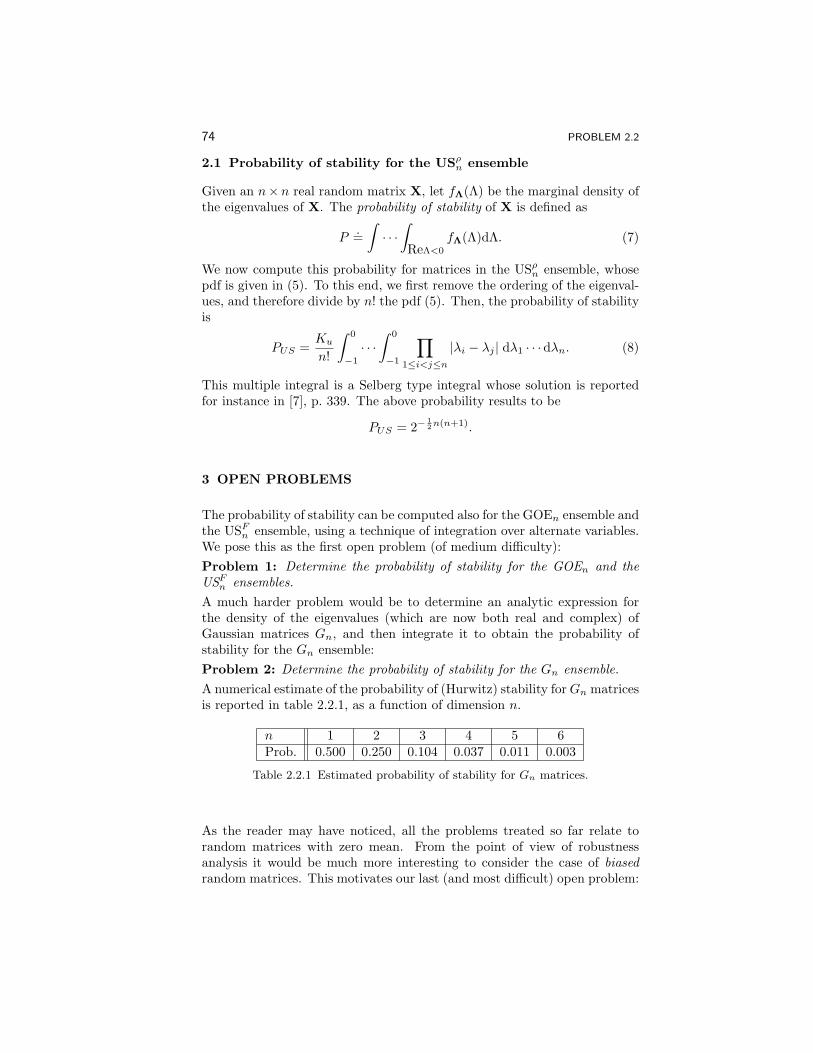
74 PROBLEM 2.2
2.1 Probability of stability for the USρn ensemble
Given an n× n real random matrix X, let fΛ(Λ) be the marginal density ofthe eigenvalues of X. The probability of stability of X is defined as
P.=∫· · ·∫ReΛ<0
fΛ(Λ)dΛ. (7)
We now compute this probability for matrices in the USρn ensemble, whosepdf is given in (5). To this end, we first remove the ordering of the eigenval-ues, and therefore divide by n! the pdf (5). Then, the probability of stabilityis
PUS =Ku
n!
∫ 0
−1
· · ·∫ 0
−1
∏1≤i<j≤n
|λi − λj | dλ1 · · ·dλn. (8)
This multiple integral is a Selberg type integral whose solution is reportedfor instance in [7], p. 339. The above probability results to be
PUS = 2−12n(n+1).
3 OPEN PROBLEMS
The probability of stability can be computed also for the GOEn ensemble andthe USFn ensemble, using a technique of integration over alternate variables.We pose this as the first open problem (of medium difficulty):Problem 1: Determine the probability of stability for the GOEn and theUSFn ensembles.A much harder problem would be to determine an analytic expression forthe density of the eigenvalues (which are now both real and complex) ofGaussian matrices Gn, and then integrate it to obtain the probability ofstability for the Gn ensemble:Problem 2: Determine the probability of stability for the Gn ensemble.A numerical estimate of the probability of (Hurwitz) stability forGn matricesis reported in table 2.2.1, as a function of dimension n.
n 1 2 3 4 5 6Prob. 0.500 0.250 0.104 0.037 0.011 0.003
Table 2.2.1 Estimated probability of stability for Gn matrices.
As the reader may have noticed, all the problems treated so far relate torandom matrices with zero mean. From the point of view of robustnessanalysis it would be much more interesting to consider the case of biasedrandom matrices. This motivates our last (and most difficult) open problem:
ON THE STABILITY OF RANDOM MATRICES 75
Problem 3: Let A ∈ Rn,n be a given stable matrix. Determine the proba-bility of stability of the random matrix A+X, where X belongs to one of theensembles listed in section 2.
ACKNOWLEDGEMENTS
The authors wish to thank Professor Madan Lal Mehta for reading andgiving his precious advice on this manuscript.
BIBLIOGRAPHY
[1] T. W. Anderson, An Introduction to Multivariate Statistical Analysis,John Wiley & Sons, New York, 1958.
[2] V. D. Blondel and J. N. Tsitsiklis, “A survey of computational complexityresults in systems and control,” Automatica, 36:1249–1274, 2000.
[3] G. Calafiore, F. Dabbene, and R. Tempo, “Randomized algorithms forprobabilistic robustness with real and complex structured uncertainty,”IEEE Trans. Aut. Control, 45(12):2218–2235, December 2000.
[4] A. Edelman, Eigenvalues and Condition Numbers of Random Matrices,Ph.D. thesis, Massachusetts Institute of Technology, Boston, 1989.
[5] A. Edelman, “How many eigenvalues of a random matrix are real?”, J.Amer. Math. Soc., 7:247–267, 1994.
[6] V. L. Girko, Theory of Random Determinants, Kluwer, Boston, 1990.
[7] M. L. Mehta, Random Matrices, Academic Press, Boston, 1991.
[8] E. P. Wigner, “Distribution laws for the roots of a random Hermitian ma-trix,” In C. E. Porter, ed., Statistical Theories of Spectra: Fluctuations.Academic, New York, 1965.
[9] E. P. Wigner, “Statistical properties of real symmetric matrices withmany dimensions,” In C. E. Porter, ed., Statistical Theories of Spectra:Fluctuations. Academic, New York, 1965.
Problem 2.3
Aspects of Fisher geometry for stochastic linear
systems
Bernard HanzonInstitute for Econometrics, Operations Research and System TheoryTechnical University of ViennaArgentinierstr. 8/119A-1040 [email protected]
Ralf PeetersDepartment of MathematicsMaastricht UniversityP.O. Box 616, 6200 MD MaastrichtThe [email protected]
1 DESCRIPTION OF THE PROBLEM
Consider the space S of stable minimum phase systems in discrete-time,of order (McMillan degree) n, having m inputs and m outputs, driven bya stationary Gaussian white noise (innovations) process of zero mean andcovariance Ω. This space is often considered, for instance in system identifi-cation, to characterize stochastic processes by means of linear time-invariantdynamical systems (see [8, 18]). The space S is well known to exhibit a dif-ferentiable manifold structure (cf. [5]), which can be endowed with a notionof distance between systems, for instance by means of a Riemannian metric,in various meaningful ways.One particular Riemannian metric of interest on S is provided by the so-called Fisher metric. Here the Riemannian metric tensor is defined in termsof local coordinates (i.e., in terms of an actual parametrization at hand) bythe Fisher information matrix associated with a given system. The openquestion raised in this paper reads as follows:
FISHER GEOMETRY FOR LINEAR SYSTEMS 77
Does there exist a uniform upper bound on the distance inducedby the Fisher metric for a fixed Ω > 0, between any two systemsin S?
In case the answer is affirmative, a natural follow-up question from the dif-ferential geometric point of view would be whether it is possible to constructa finite atlas of charts for the manifold S, such that the charts as subsets ofEuclidean space are bounded (i.e., contained in an open ball in Euclideanspace), while the distortion of each chart remains finite.
2 MOTIVATION AND BACKGROUND OF THE PROBLEM
An important and well-studied problem in linear systems identification isthe construction of parametrizations for various classes of linear systems. Inthe literature a great number of parametrizations for linear systems havebeen proposed and used. From the geometric point of view the questionarises whether one can qualify various parametrizations as good or bad. Aparametrization is a way to (locally) describe a geometric object. Intuitively,a parametrization is better the more it reflects the (local) structure of thegeometric object. An important consideration in this respect is the scale ofthe parametrization, or rather the spectrum of scales, see [4]. To explainthis, consider the tangent space of a differential manifold of systems, such asS. The differentiable manifold can be supplied with a Riemannian geometry,for example, by smoothly embedding the differentiable manifold in an ap-propriate Hilbert space: then the tangent spaces to the manifold are linearsubspaces of the Hilbert space, which induces an inner product on each of thetangent spaces and a Riemannian metric structure on the manifold. If such aRiemannian metric is defined, then any sufficiently smooth parametrizationwill have an associated Riemannian metric tensor. In local coordinates (i.e.,in terms of the parameters used) it is represented by a symmetric, positivedefinite matrix at each point. The eigenvalues of this matrix reflect the lo-cal scales of the parametrization: the scale of any infinitesimal movementstarting from a given point, will vary between the largest and the smallesteigenvalue of the Riemannian metric tensor at the point involved. Over aset of points the scale will clearly vary between the largest eigenvalue to befound in the spectra of the corresponding set of Riemannian metric matricesand the smallest eigenvalue to be found in that same set of spectra. Follow-ing Milnor (see [12]), who considered the question of finding good charts forthe earth, we define the distortion of a parametrization, which we will callthe Milnor distortion, as the quotient of the largest scale and the smallestscale of the parametrization.Note that this concept of Milnor distortion is a generalization of the conceptof the condition number of a matrix. However it is (in general) not themaximum of the condition numbers of the set of Riemannian metric matrices.

78 PROBLEM 2.3
Indeed, the largest eigenvalue and the smallest eigenvalue that enter intothe definition of the Milnor distortion do not have to correspond to theRiemannian metric tensor at the same point.If one has an atlas of overlapping charts, one can calculate the Milnor dis-tortion in each of the charts and consider the largest distortion in any of thecharts of the atlas. One could now be tempted to define this number as thedistortion of the atlas and look for atlases with relatively small distortion.However, in this case, the problem shows up that it is always possible to takea large number of small charts, each one displaying very little distortion (i.e.,distortion close to one), while such an atlas may still not be desirable as itmay require a huge number of charts. The difficulty here is to trade off thenumber of charts in an atlas against the Milnor distortion in each of thosecharts. At this point, we have no clear natural candidate for this trade-off.But at least for atlases with an equal finite number of charts the concept ofmaximal Milnor distortion could be used to compare the atlases.
3 AVAILABLE RESULTS
In trying to apply these ideas to the question of parametrization of lin-ear systems, the problem arises that many parametrizations turn out tohave in fact an infinite Milnor distortion. Consider for example the caseof real SISO discrete-time strictly proper stable systems of order one. (Seealso [9] and [13, section 4.7].) This set can be described by two real pa-rameters, e.g., by writing the associated transfer function into the formh(z) = b/(z − a). Here, the parameter a denotes the pole of the systemand the parameter b is associated with the gain. The Riemannian metrictensor induced by the H2 norm of this parametrization can be computed
as(b2(1 + a2)/(1− a2)3 ab/(1− a2)2
ab/(1− a2)2 1/(1− a2)
), see [9]. Therefore it tends to
infinity when a approaches the stability boundary |a| = 1, whence the Mil-nor distortion of this parametrization becomes infinity. In this example thegeometry is that of a flat double infinite-sheeted Riemann surface. Locally,it is isometric with Euclidean space and therefore one can construct chartsthat have the identity matrix as their Riemannian metric tensor (see [13]).However, in this case, this means that close to the stability boundary thedistances between points become arbitrarily large. Therefore, although it ispossible to construct charts with optimal Milnor distortion, this can only bedone at the price of having to work with infinitely large (i.e., unbounded)charts. If one wants to work with charts in which the distances remainbounded then one will need infinitely many of them on such occasions.In the case of stochastic Gaussian time-invariant linear dynamical systemswithout observed inputs, the class of stable minimum-phase systems plays animportant role. For such stochastic systems the (asymptotic) Fisher informa-tion matrix is well-defined. This matrix is dependent on the parametrization
FISHER GEOMETRY FOR LINEAR SYSTEMS 79
used and admits the interpretation of a Riemannian metric tensor (see [15]).There is an extensive literature on the computation of Fisher information,especially for AR and ARMA systems. See, e.g., [6, 7, 11]. Much of thisinterest derives from the many applications in practical settings: it can beused to establish local parameter identifiability, it is used for parameter es-timation in the method of scoring, and it is also known to determine thelocal convergence properties of the popular Gauss-Newton method for least-squares identification of linear systems based on the maximum likelihoodprinciple (see [10]).In the case of stable AR systems, the Fisher metric tensor can, for instance,be calculated using the parametrization with Schur parameters. From theformulas in [14] it follows that the Fisher information for scalar AR systemsof order one driven by zero mean Gaussian white noise of unit variance isequal to 1/(1 − γ2
1). Here γ1 is required to range between −1 and 1 (toimpose stability) and to be nonzero (to impose minimality). Although thisagain implies an infinite Milnor distortion, the situation here is structurallydifferent from the situation in the previous case: the length of the curveof systems obtained by letting γ1 range from 0 to 1 is finite! Indeed, the(Fisher) length of this curve is computed as
∫ 1
01√
1−γ21
dγ1 = π/2.
Let the inner geometry of a connected Riemannian manifold of systems bedefined by the shortest path distance: d(Σ1,Σ2) is the Riemannian lengthof the shortest curve connecting the two systems Σ1 and Σ2. Then, in thissimple case, the Fisher geometry has the property that the correspondinginner geometry has a uniform upper bound. Therefore, this example providesan instance of a subset of the manifold S for which the answer to the questionraised is affirmative.As a matter of fact, if one now reparametrizes the set of systems as in [17] byθ defined through γ1 = sin(θ), then the resulting Fisher information quantitybecomes equal to 1 everywhere. Thus, it is bounded and the Milnor distor-tion of this reparametrization is finite. But at the same time the parameterchart itself remains bounded! Hence, also the “follow-up question” of theprevious section is answered affirmative here.If one considers SISO stable minimum-phase systems of order 1, it can beshown likewise that also here the Fisher distance between two systems isuniformly bounded and that a finite atlas with bounded charts and finiteMilnor distortion can be designed. Whether this also occurs for larger state-space dimensions is still unknown (to the best of the authors’ knowledge)and this is precisely the open problem presented above.To conclude, we note that the role played by the covariance matrix Ω of thedriving white noise is rather limited. It is well known that if the systemequations and the covariance matrix are parametrized independently of eachother, then the Fisher information matrix attains a block-diagonal structure(see, e.g., [18, Ch. 7]. The covariance matrix Ω then appears as a weightingmatrix for the block of the Fisher information matrix associated with the
80 PROBLEM 2.3
parameters involved in the system equations. Therefore, if Ω is known, orrather if an upper bound on Ω is known (which is likely to be the case inany practical situation!), its role with respect to the questions raised can belargely disregarded. This allows to restrict attention to the situation whereΩ is fixed to the identity matrix Im.
BIBLIOGRAPHY
[1] S.-I. Amari, Differential-Geometrical Methods in Statistics, LectureNotes in Statistics 28, Springer Verlag, Berlin, 1985.
[2] S.-I. Amari, “Differential geometry of a parametric family of invertiblelinear systems Riemannian metric, dual affine connections, and diver-gence,” Mathematical Systems Theory, 20, 53–82, 1987
[3] C. Atkinson and A. F. S. Mitchell, “Rao’s distance measure. Sankhya:The Indian Journal of Statistics, Series A, 43(3), 345–365, 1981.
[4] R. W. Brockett and P. S. Krishnaprasad “A scaling theory for linearsystems,” IEEE Trans. Aut. Contr., AC-25, 197–206, 1980.
[5] J. M. C. Clark, “The consistent selection of parametrizations in sys-tem identification,” Proc. Joint Automatic Control Conference, 576–580. Purdue University, Lafayette, Indiana, 1976.
[6] B. Friedlander, “On the Computation of the Cramer-Rao Boundfor ARMA Parameter Estimation,” IEEE Transactions on Acoustics,Speech and Signal Processing, ASSP-32 (4), 721–727.
[7] E. J. Godolphin and J. M. Unwin, “Evaluation of the covariance matrixfor the maximum likelihood estimator of a Gaussian autoregressive-moving average process,” Biometrika, 70 (1), 279–284, 1983.
[8] E. J. Hannan and M. Deistler, The Statistical Theory of Linear Systems.John Wiley & Sons, New York, 1988.
[9] B. Hanzon, Identifiability, Recursive Identification and Spaces of LinearDynamical Systems, CWI Tracts 63 and 64, Centrum voor Wiskundeen Informatica (CWI), Amsterdam, 1989.
[10] B. Hanzon and R. L. M. Peeters, “On the Riemannian Interpreta-tion of the Gauss-Newton Algorithm,” In: M. Karny and K. Warwick(eds.), Mutual Impact of Computing Power and Control Theory, 111–121. Plenum Press, New York, 1993.
[11] A. Klein and G. Melard,“On Algorithms for Computing the Covari-ance Matrix of Estimates in Autoregressive Moving Average Processes,”Computational Statistics Quarterly, 1, 1–9, 1989.
FISHER GEOMETRY FOR LINEAR SYSTEMS 81
[12] J. Milnor, “A problem in cartography,” American Math. Monthly, 76,1101–1112, 1969.
[13] R. L. M. Peeters, System Identification Based on Riemannian Geome-try: Theory and Algorithms. Tinbergen Institute Research Series, vol.64, Thesis Publishers, Amsterdam, 1994.
[14] R. L. M. Peeters and B. Hanzon, “Symbolic computation of Fisher in-formation matrices for parametrized state-space systems,” Automatica,35, 1059–1071, 1999.
[15] C. R. Rao, “Information and accuracy attainable in the estimation ofstatistical parameters,” Bull. Calcutta Math. Soc., 37, 81–91, 1945.
[16] N. Ravishanker, E. L. Melnick and C.-L. Tsai, “Differential geometryof ARMA models,” Journal of Time Series Analysis, 11, 259–274, .
[17] A. L. Rijkeboer, “Fisher optimal approximation of an AR(n)-process byan AR(n-1)-process,” In: J. W. Nieuwenhuis, C. Praagman and H. L.Trentelman eds., Proceedings of the 2nd European Control ConferenceECC ’93, 1225–1229, Groningen, 1993.
[18] T. Soderstrom and P. Stoica, System Identification, Prentice-Hall, NewYork, 1989.
Problem 2.4
On the convergence of normal forms for analytic
control systems
Wei KangDepartment of Mathematics,Naval Postgraduate SchoolMonterey, CA [email protected]
Arthur J. KrenerDepartment of Mathematics,University of CaliforniaDavis, CA [email protected]
1 BACKGROUND
A fruitful technique for the local analysis of a dynamical system consists ofusing a local change of coordinates to transform the system to a simpler form,which is called a normal form. The qualitative behavior of the original systemis equivalent to that of its normal form which may be easier to analyze.A bifurcation of a parameterized dynamics occurs when a change in theparameter leads to a change in its qualitative properties. Therefore, normalforms are useful in analyzing when and how a bifurcation will occur. Inhis dissertation, Poincare studied the problem of linearizing a dynamicalsystem around an equilibrium point, linear dynamics being the simplestnormal form. Poincare’s idea is to simplify the linear part of a system first,using a linear change of coordinates. Then the quadratic terms in the systemare simplified, using a quadratic change of coordinates, then the cubic terms,and so on. For systems that are not linearizable, the Poincare-Dulac theoremprovides the normal form.Given a C∞ dynamical system in its Taylor expansion around x = 0,
x = f(x) = Fx+ f [2](x) + f [3](x) + · · · (1)
CONVERGENCE OF NORMAL FORMS 83
where x ∈ <n, F is a diagonal matrix with eigenvalues λ = (λ1, . . . , λn), andf [d](x) is a vector field of homogeneous polynomial of degree d. The dots+ · · · represent the rest of the formal power series expansion of f . Let ekbe the k-th unit vector in <n. Let m = (m1, . . . ,mn) be a vector of non-negative integers. In the following, we define |x| and xm by |m| =
∑|mi|
and xm = xm11 xm2
2 . . . xmnn . A nonlinear term xmek is said to be resonant
if m · λ = λk for some nonzero vector of non-negative integers m and some1 ≤ k ≤ n .
Definition 1 The eigenvalues of F are in the Poincare domain if their convexhull does not contain zero, otherwise they are in the Siegel domain.
Definition 2: The eigenvalues of F are of type (C, ν) for some C > 0, ν > 0if
|m · λ− λk| ≥C
|m|ν
For eigenvalues in the Poincare domain, there are at most a finite numberof resonances. For eigenvalues of type (C, ν), there are no resonances and as|m| → ∞ the rate at which resonances are approached is controlled.A formal change of coordinates is a formal power series
z = Tx+ θ[2](x) + θ[3](x) + · · · (2)
where T is invertible. If T = I, then it is called a near identity changeof coordinates. If the power series converges locally, then it defines a realanalytic change of coordinates.
Theorem 1: (Poincare-Dulac) If the system (1) is C∞ then there exists aformal change of coordinates (2) transforming it to
z = Az + w(z)
where A is in Jordan form and w(z) consists solely of resonant terms. (Ifsome of the eigenvalues of F are complex then the change of coordinates willalso be complex). In this normal form, w(z) need not be unique.If the system (1) is real analytic and its eigenvalues lie in the Poincare do-main (2), then w(z) is a polynomial vector field and the change of coordinates(2)is real analytic.
Theorem 2: (Siegel) If the system (1) is real analytic and its eigenvaluesare of type (C, ν) for some C > 0, ν > 0 , then w(z) = 0 and the change ofcoordinates (2) is real analytic.
As is pointed out in [1], even in cases where the formal series are divergent,the method of normal forms turns out to be a powerful device in the studyof nonlinear dynamical systems. A few low degree terms in the normal formoften give significant information on the local behavior of the dynamics.
84 PROBLEM 2.4
2 THE OPEN PROBLEM
In [3], [4], [5], [10], and [8], Poincare’s idea is applied to nonlinear control sys-tems. A normal form is derived for nonlinear control systems under changeof state coordinates and invertible state feedback. Consider a C∞ controlsystem
x = f(x, u) = Fx+Gu+ f [2](x, u) + f [3](x, u) + · · · (3)where x ∈ <n is the state variable, u ∈ < is a control input. We only discussscalar input systems, but the problem can be generalized to vector inputsystems. Such a system is called linearly controllable at the origin if thelinearization (F,G) is controllable.In contrast with Poincare’s theory, a homogeneous transformation for (3)consists of both change of coordinates and invertible state feedback,
z = x+ θ[d](x), v = u+ κ[d](x, u) (4)
where θ[d](x) represents a vector field whose components are homogeneouspolynomials of degree d. Similarly, κ[d](x) is a polynomial of degree d. Aformal transformation is defined by
z = Tx+∑∞d=2 θ
[d](x), v = Ku+∑∞d=2 κ
[d](x, u) (5)where T and K are invertible. If T and K are identity matrices then this iscalled a near identity transformation.The following theorem for the normal form of control systems is a slightgeneralization of that proved in [3], see also [8] and [10].
Theorem 3: Suppose (F,G) in (3) is a controllable pair. Under a suitabletransformation (5), (3) can be transformed into the following normal form
zi = zi+1 +∑n+1j=i+2 pi,j(zj)z
2j 1 ≤ i ≤ n− 1
zn = v(6)
where zn+1 = v, zj = (z1, z2, · · · , zj), and pi,j(zj) is a formal series of zj.
Once again, the convergence of the formal series pi,j in (6) is not guaranteed,hence nothing is known about the convergence of the normal form.
Open Problem (The Convergence of Normal Form): Suppose the con-trolled vector field f(x, u) in (3) is real analytic and F,G is a controllablepair. Find verifiable necessary and sufficient conditions for the existence ofa real analytic transformation (5) that transforms the system to the normalform (6).
Normal forms of control systems have proven to be a powerful tool in theanalysis of local bifurcations and local qualitative performance of controlsystems. A convergent normal form will make it possible to study a controlsystem over the entire region in which the normal form converges. Globalor semi-global results on control systems and feedback design can be provedby studying analytic normal forms.

CONVERGENCE OF NORMAL FORMS 85
3 RELATED RESULTS
The convergence of the Poincare normal form was an active research topic indynamical systems. According to Poincare’s Theorem and Siegel’s theorem,the location of eigenvalues determines the convergence. If the eigenvaluesare located in the Poincare domain with no resonances, or if the eigenvaluesare located in the Siegel domain and are of type (C, ν), then the analyticvector field that defines the system is biholomorphically equivalent to a linearvector field. Clearly, the normal form converges because it has only a linearpart. The Poincare-Dulac theorem deals with a more complicated case. Itstates that if the eigenvalues of an analytic vector field belong to the Poincaredomain, then the field is biholomorphically equivalent to a polynomial vectorfield. Therefore, the Poincare normal form has only finite many terms, andhence is convergent.As for control systems, it is proved in [5] that if an analytic control systemis linearizable by a formal transformation, than it is linearizable by an ana-lytic transformation. It is also proved in [5] that a class of three-dimensionalanalytic control systems, which are not necessarily linearizable, can be trans-formed to their normal forms by analytic transformations. No other resultson the convergence of control system normal forms are known to us.The convergence problem for control systems has a fundamental differencefrom the convergence results of Poincare-Dulac. For the latter, the locationof the eigenvalues are crucial and the eigenvalues are invariant under changeof coordinates. However, the eigenvalues of a control system can be changedby linear state feedback. It is unknown what intrinsic factor in controlsystems determines the convergence of their normal form or if the normalform is always convergent.The convergence of normal forms is an important problem to be addressed.Applications of normal forms for control systems are proved to be successful.In [6] the normal forms are used to classify the bifurcation of equilibriumsets and controllability for uncontrollable systems. In [7] the control ofbifurcations using state feedback is introduced based on normal forms. Fordiscrete-time systems, normal form and the stabilization of Naimark-Sackerbifurcation are addressed in [2]. In [10] a complete characterization for thesymmetry of nonlinear systems is found for linearly controllable systems.In addition to linearly controllable systems, the normal form theory has beengeneralized to larger family of control systems. Normal forms for systemswith uncontrollable linearization are derived in several papers ([6], [7], [8],and [10]). Normal forms of discrete-time systems can be found in [9] and [2].The convergence of these normal forms is also an open problem.
86 PROBLEM 2.4
BIBLIOGRAPHY
[1] V. I. Arnold, Geometrical Method in the Theory of Ordinary DifferentialEquations, Springer-Verlag, New York, Berlin, 1988.
[2] B. Hamzi, J.-P. Barbot, S. Monaco, and D. Normand-Cyrot, “Nonlineardiscrete-time control of systems with a Naimark-Sacker bifurcation,”Systems and Control Letters, 44, 4, pp. 245-258, 2001.
[3] W. Kang, Extended controller normal form, invariants and dynamicalfeedback linearization of nonlinear control systems, Ph.D. dissertation,University of California at Davis, 1991.
[4] W. Kang and A. J. Krener, “Extended quadratic controller normalform and dynamic feedback linearization of nonlinear systems,” SIAMJ. Control and Optimization, 30 (1992), 1319-1337.
[5] W. Kang, “Extended controller form and invariants of nonlinear controlsystems with a single input,” J. of Mathematical Systems, Estimationand Control, 6 (1996), 27-51.
[6] W. Kang, “Bifurcation and normal form of nonlinear control systems -Part I and II, SIAM J. Control and Optimization, 36 (1998), 193-212and 213-232.
[7] W. Kang, “Bifurcation control via state feedback for systems with asingle uncontrollable mode,” SIAM J. Control and Optimization, 38,(2000), 1428-1452.
[8] A. J. Krener, W. Kang, and D. E. Chang, “Control bifurcations,” IEEETransactions on Automatic Control, forthcoming.
[9] A. J. Krener and L. Li, “Normal forms and bifurcations of discrete timenonlinear control systems,” Proc. of 5th IFAC NOLCOS Symposium,Saint-Petersburg, 2001.
[10] I. Tall and W. Respondek, “Feedback classification of nonlinear single-input controls systems with controllable linearization: Normal forms,canonical forms, and invariants,” preprint.

PART 3
Nonlinear Systems


Problem 3.1
Minimum time control of the Kepler equation
Jean-Baptiste Caillau, Joseph Gergaud,and Joseph NoaillesENSEEIHT-IRIT, UMR CNRS 55052 rue CamichelF-31071 ToulouseFrancecaillau, gergaud, [email protected]
1 DESCRIPTION OF THE PROBLEM
We consider the controlled Kepler equation in three dimensions
r = −k r
|r|3+ γ (1)
where r = (r1, r2, r3) is the position vector–the double dot denoting thesecond order time derivative–, k a strictly positive constant, |.| the Euclideannorm in R3, and where γ = (γ1, γ2, γ3) is the control. The minimum timeproblem is then stated as follows: find a positive time T and a measurablefunction γ defined on [0, T ] such that (1) holds almost everywhere on [0, T ]and:
T → minr(0) = r0, r(0) = r0 (2)h(r(T ), r(T )) = 0 (3)
|γ| ≤ Γ. (4)
In (2), r0 and r0 are the known initial position and speed with:
|r0|2
2− k
|r0|< 0
in order that the uncontrolled initial motion be periodic [1]. In (3) h isa fixed submersion of R6 onto Rl, l ≤ 6, defining a non-trivial endpointcondition. The constraint (4) on the Euclidean norm of the control, with Γa strictly positive constant, means that almost everywhere on [0, T ]
γ21 + γ2
2 + γ23 ≤ Γ2.
90 PROBLEM 3.1
Our first concern is uniqueness (see §3 about existence):
Question 1. Is the optimal control unique?
The second point is about regularity, namely:
Question 2. Are there continuous optimal controls?
Denoting by T (Γ) the value function that assigns to any strictly positive Γ(parameter involved in (4)) the associated minimum time, our third and lastquestion is:
Question 3. Does the product T (Γ) · Γ have a limit when Γ tends to zero?
2 MOTIVATION
This problem originates in the computation of optimal orbit transfers incelestial mechanics for satellites with very low thrust engines [5]. Since the1990s, low electro-ionic propulsion is been considered as an alternative tostrong chemical propulsion, but the lower the thrust, the longer the transfertime, hence the idea of minimizing the final time. In this context, γ is theratio u/m of the engine thrust by the mass of the satellite, and one hasmoreover to take into account the mass variation due to fuel consumption:
m = −β|u|.
Typical boundary conditions in this case consist in inserting the spacecrafton a high geostationnary orbit, and the terminal condition is defined by:
|r(T )| and |r(T )| fixed, r(T ) · r(T ) = 0, r(T )× r(T )× ~k = 0
where ~k is the normal vector to the equatorial plane.
In contrast with the impulsional manoeuvres performed using the strongclassic chemical propulsion, the gradual control by a low thrust engine issometimes referred to as “continuous?” Thus, question 2 could be rephrasedaccording to:
Are “continuous” optimal controls continuous?
Besides, this question is also relevant in practice since continuity of controlsis the basic assumption required by most numerical methods [2]. In thesame respect, question 3 is the key to get accurate estimates of the unknowntransfer time, needed to ensure convergence of the numerical computation.
MINIMUM TIME CONTROL OF THE KEPLER EQUATION 91
3 RELATED RESULTS
The existence of controls achieving the minimum time transfer comes fromthe controllability of the system (the associated Lie algebra has maximalrank and the drift is periodic, see [7]) and from the convexity properties ofthe dynamics by Filippov theorem [4]. Regarding regularity, it is proven in[3] (whose results extend straightforwardly to three dimensions) that anytime minimal control of (1) has at most finitely many discontinuity points.More precisely, using Pontryagin Maximum Principle [4, 6], one gets thatany discontinuity point t is a switching point in the sense that the control isinstantaneously rotated of an angle π:
γ(t+) = −γ(t−).Furthermore, bounds are given in [3], not on the total number of switch-ings but for those located at special points of the osculating ellipse: therecannot be consecutive switchings at perigee or apogee. Since the numericssuggest that the possible discontinuities are exactly located at the perigee,a conjecture would be:
There is at most one switching point and this point is located at the perigee.
Finally, as for question 3, the value function T (Γ) is obviously decreasingand is proven to be right-continuous in [2]. Besides, the product T (Γ) · Γturns to be nearly constant numerically so that the conjecture would be toanswer positively:
There is a positive constant c such that T (Γ) · Γ tends to c when Γtends to zero.
BIBLIOGRAPHY
[1] V. I. Arnold, Mathematical Methods of Classical Mechanics, Springer-Verlag, 1978.
[2] J. B. Caillau, J. Gergaud and J. Noailles, “3D geosynchronous transferof a satellite: Continuation on the thrust,” JOTA, 118:3, 2003 (Forth-coming).
[3] J.B. Caillau and J. Noailles, “Coplanar control of a satellite around theearth,” ESAIM COCV, vol. 6, pp. 239-258, 2001.
[4] L. Cesari,Optimization Theory and Applications, Springer-Verlag, 1983.
[5] J. Noailles and C. T. Le, “Controle en temps minimal et transfert afaible poussee,” Equations aux derivees partielles et applications, Articlesin Honour of J. L. Lions for his 70th Birthday, pp. 705-724, Gauthiers-Villars, 1998.
92 PROBLEM 3.1
[6] H. J. Sussmann, “Geometry and optimal control,” Mathematical ControlTheory, Dedicated to R. W. Brockett on his 60th Birthday, J. Baillieuland J. C. Willems eds., Springer-Verlag, 1998.
[7] V. Jurdjevic,Geometric Control Theory Cambridge University Press,1997.

Problem 3.2
Linearization of linearly controllable systems
R. DevanathanSchool of Electrical and Electronic Engineering (Block S1)Nanyang Technological UniversitySingapore 639798Republic of [email protected]
1 DESCRIPTION OF THE PROBLEM
We consider a class of systems of the form
ξ = f(ξ) + g(ξ)ζ (1)
where ξ is an n-tuple vector and f(ξ)and g(ξ) are vector fields, i.e., n-tuple vectors whose elements are, in general, functions of ξ. For simplicity,we assume a scalar input ζ. We require that the system (1) be linearlycontrollable [1], i.e., the pair (F,G) is controllable where F = ∂f
∂ξ (0) andG = g(0) at the assumed equilibrium point at the origin.The power series expansion of (1) about the origin can be written, with anappropriate change of variable and input, as
x = Fx+Gφ+O1(x)(2) + γ1(x, φ)(1) (2)
where, without loss of generality, F and G can be in Brunovsky form [2],superscript (2) corresponds to terms in x of degree greater than one, super-script (1) corresponds to terms in x of degree greater than or equal to oneand x and φ are the transformed state and input variables respectively. Weintroduce state feedback as in [3]
φ = −Kx+ u
where
K = [kn, kn−1, · · · , k2, k1]t
Equation (2) then becomes
x = Ax+Gu+O(x)(2) + γ(x, u)(1) (3)

94 PROBLEM 3.2
whereA = F −GK (4)
We can choose the eigenvalues of matrix A in (4), without loss of generality,to be real, distinct, and nonresonant by a proper choice of the matrix K [3].The nonresonant property, meaning that no integral relation exists amongthe eigenvalues of matrix A, ensures that (3) can be linearized up to anarbitrary order.Put (3) into the form
x = Ax+Gu+ f2(x) + f3(x) + · · ·+ g1(x)u+ g2(x)u+ · · · (5)where fm(x) and gm−1(x) correspond to vector-valued polynomials contain-ing terms of the form
xm = xm11 xm2
2 · · · xmnn , mi ∈ (0, 1, 2, · · · , n), i = 1, 2, · · · , n;n∑i=1
mi = m,m ≥ 2.
Consider a near identity (normalizing) transformation as inx = y + h(y) (6)
and a change of input as inv = (1 + β(x))u+ α(x) , 1 + β(x) 6= 0 (7)
whereh(y) = h2(y) + h3(y) + · · · (8)α(x) = α2(x) + α3(x) + · · · (9)β(x) = β1(x) + β2(x) + · · · (10)
The problem is to find a solution for hm(.), αm(.) and βm−1(.), m ≥ 2such that the nonlinear terms upto an arbitrary order, viz., “fm(.)” and“gm−1(.)u” can be removed from (5) by the application of the transforma-tions (6) and (7) to it.
2 MOTIVATION AND HISTORY OF THE PROBLEM
Linearization of a nonlinear dynamic system of the form (1), but without thecontrol input, was originally investigated by Poincar [4] [5]. It was shownthat, around an equilibrium point, a near identity (normalizing ) transfor-mation takes it to its normal form where only the residual nonlinearities, thatcannot be removed by the transformation, remain. The dynamic system issaid to be resonant in the order of these residual nonlinearities.The solution for the normalizing transformation is in the form of an infiniteseries as in (8) whose convergence has been proved under certain assumptions[6] [7]. Irrespective of the convergence of the infinite series, the transforma-tion is of interest because, one can remove up to an arbitrary order of non-linearities (as long as they are nonresonant) through such a transformation,thus providing an approximate linearization of the dynamic system.
LINEARIZATION OF LINEARLY CONTROLLABLE SYSTEMS 95
3 AVAILABLE RESULTS
Our problem is an analog of Poincar’s problem with the control input pro-vided. Krener et al. [8] have considered a nonlinear system of the form(1) and showed that a generalized form of the homological equation can beformulated in this case. Devanathan [3] has shown that, for a linearly con-trollable system, the system matrix can be made nonresonant through anappropriate choice of state feedback. This concept is further exploited in [9]to find a solution to the second order linearization. An analogous solutionto the case of an arbitrary order linearization, however, is still open.By application of (6) and (7), one can write
f2(x) + f3(x) + f4(x) + · · ·= f ′2(y) + f ′3(y) + f ′4(y) + · · · (11)g1(x)u+ g2(x)u+ g3(x)u+ · · ·= g′1(y)u+ g′2(y)u+ g′3(y)u+ · · · (12)
α(x) =α′2(y) + α′3(y) + α′4(y) + · · · (13)β(x) =β′1(y) + β′2(y) + β′3(y) + · · · (14)
for some appropriate polynomials f ′m(.), g′m−1(.), α′m(.) and β′m−1(.),m ≥ 2.
Substituting (6) and (7) into (5) and using (11)-(14), consider the polyno-mials of the form ym and ym−1u, m = 2, 3, · · · . Then the terms “fm(x)”and “gm−1(x)u” can be removed from (5) progressively, m = 2,3, etc. pro-vided the following generalized homological equations are satisfied [3].
∂hm(y)∂y
(Ay)−Ahm(y) +Gα′m(y) = f ′′m(y),m ≥ 2 (15)
∂hm(y)∂y
(Gu) +Gβ′m−1(y)u = g′′m−1(y)u, ∀u,m ≥ 2 (16)
where f ′′2 (y) = f ′2(y) = f2(y) and f ′′m(y) is expressed in terms of f ′m−i(y), i =0, 1, 2, · · · , (m− 2) and hm−j(y),j = 1, 2, · · · , (m− 2), m > 2. Also, g′′1 (y) =g′1(y) = g1(y) and g′′m(y) is expressed in terms of g′m−i(y), i = 0, 1, 2, · · · , (m−1) and hm−j(y),j = 0, 1, 2, · · · , (m− 2), m ≥ 2.Assuming that hm−j(y), αm−j(y), βm−j−1(y), j = 1, 2, · · · , (m− 2), m > 2 ,are known, f ′′m(y) and g′′m−1(y) can be computed. Without loss of generality,one can assume matrix A to be diagonal and G = [1, 1, · · · , 1, 1]t by applyinga change of coordinate to (5) involving Vandermonde matrix [10]. Onecan then proceed to solve (15) for hm(y) in terms of αm(y) and substitutethe same into (16) to set up a linear system of equations in the unknowncoefficients of polynomials αm(y) and βm−1(y).For m = 2, it has been shown in [9] that the corresponding system of linearequations can be reduced to a system of (n(n−1)
2 ) equations in n variableswhose rank is (n− 1). It is conjectured that a similar reduction of the linearsystem of equations, in the arbitrary order case, should also be possible.Formulation of the properties and solution, if it exists, of the linear systemof equations involving the coefficients of the polynomials αm(.), βm−1(.) andhm(.),m > 2 will constitute the solution to the open problem.
96 PROBLEM 3.2
BIBLIOGRAPHY
[1] A. J. Krener and W. Kang, “Extended normal forms of quadratic sys-tems,” Proc. 29th Conf. Decision and Control, pp. 2091-2095, 1990.
[2] P. Brunovsky, “A Classification of linear controllable systems,” Kyber-netica cislo, vol. 3, pp. 173-188, 1970.
[3] R. Devanathan, “Linearization condition through state feedback,” IEEETransactions on Automatic Control, vol. 46, no. 8, pp. 1257-1260, 2001.
[4] V. I. Arnold, Geometrical Methods in the Theory of Ordinary DifferentialEquations, Springer-Verlag, New York, pp. 177-188, 1983.
[5] J. Guckenheimer and P. Holmes, Nonlinear Oscillations, Dynamical Sys-tems and Bifurcation of Vector Fields, Springer-Verlag, New York, 1983.
[6] A. D. Bruno, Local Methods in Nonlinear Differential Equations,Springer-Verlag, Berlin, 1989.
[7] Giampaolo Cicogna, “On the convergence of normalizing transformationsin the presence of symmetries,” Departmento di Fisica, Universita diPisa, P.za Torricelli 2, I-56126, Pisa, Italy.
[8] A. J. Krener, S. Karahan, and M. Hubbard, “Approximate normal formsof nonlinear systems,” Proc. 27th Conf. Decision and Control, pp. 1223-1229, 1988.
[9] R. Devanathan, “Solution of second order linearization,” Fifteenth Inter-national Symposium on Mathematical Theory of Networks and Systems,University of Notre Dame, Notre Dame, IN,USA (2002).
[10] B. C. Kuo, Automatic Control Systems, Fourth Ed., Prentice-Hall, pp.227-240, 1982.
Problem 3.3
Bases for Lie algebras and a continuous CBH formula
Matthias Kawski1Department of Mathematics and StatisticsArizona State UniversityTempe, AZ [email protected]
1 DESCRIPTION OF THE PROBLEM
Many time-varying linear systems x = F (t, x) naturally split into time-invariant geometric components and time-dependent parameters. A specialcase are nonlinear control systems that are affine in the control u, and spec-ified by analytic vector fields on a manifold Mn
x = f0(x) +m∑k=1
uk fk(x). (1)
It is natural to search for solution formulas for x(t) = x(t, u) that separatethe time-dependent contributions of the controls u from the invariant, ge-ometric role of the vector fields fk. Ideally, one may be able to a prioriobtain closed-form expressions for the flows of certain vector fields. Thequadratures of the control might be done in real-time, or the integrals of thecontrols may be considered new variables for theoretical purposes such aspath-planning or tracking.To make this scheme work, one needs simple formulas for assembling thesepieces to obtain the solution curve x(t, u). Such formulas are nontrivial sincein general the vector fields fk do not commute: already in the case of linearsystems, exp(sA) · exp(tB) 6= exp(sA + tB) (for matrices A and B). Thusthe desired formulas not only involve the flows of the system vector fields fibut also the flows of their iterated commutators [fi, fj ], [[fi, fj ], fk], and soon.Using Hall-Viennot bases H for the free Lie algebra generated by m inde-terminates X1, . . . Xm, Sussmann [22] gave a general formula as a directed
1Supported in part by NSF-grant DMS 00-72369
98 PROBLEM 3.3
infinite product of exponentials
x(T, u) =→∏
H∈H
exp(ξH(T, u) · fH). (2)
Here the vector field fH is the image of the formal bracket H under thecanonical Lie algebra homomorphism that maps Xi to fi. Using the chrono-logical product (U ∗ V )(t) =
∫ T0U(s)V ′(s) ds, the iterated integrals ξH are
defined recursively by ξXk(T, u) =
∫ T0uk(t)dt and
ξHK = ξH ∗ ξK (3)
if H,K,HK are Hall words and the left factor of K is not equal to H [9,22]. (In the case of repeated left factors, the formula contains an additionalfactorial.)
An alternative to such infinite exponential product (in Lie group language,“coordinates of the 2nd kind”) is a single exponential of an infinite Lie series(“coordinates of the 1st kind”).
x(T, u) = exp(∑B∈B
ζB(T, u) · fB) (4)
It is straightforward to obtain explicit formulas for ζB for some spanningsets B of the free Lie algebra [22], but much preferable are series that usebases B, and which, in addition, yield as simple formulas for ζB as (3) doesfor ξH .
Problem 1: Construct bases B = Bk : k ≥ 0 for the free Lie algebra on afinite number of generators X1, . . . Xm such that the corresponding iteratedintegral functionals ζB defined by (4) have simple formulas (similar to (3)),suitable for control applications (both analysis and design).
The formulae (4) and (2) arise from the “free control system” on the freeassociative algebra on m generators. Its universality means that its solutionsmap to solutions of specific systems (1) on Mn via the evaluation homomor-phism Xi 7→ fi. However, the resulting formulas contain many redundantterms since the vector fields fB are not linearly independent.
Problem 2: Provide an algorithm that generates for any finite collectionof analytic vector fields F = f1, . . . , fm on Mn a basis for L(f1, . . . , fm)together with effective formulas for associated iterated integral functionals.
Without loss of generality, one may assume that the collection F satisfiesthe Lie algebra rank condition, i.e., L(f1, . . . , fm)(p) = TpM at a specifiedinitial point p. It makes sense to first consider special classes of systems F,e.g., which are such that L(f1, . . . , fm) is finite, nilpotent, solvable, etc. Thewords simple and effective are not used in a technical sense in problems 1and 2 (as in formal studies of computational complexity) but instead referto comparison with the elegant formula (3), which has proven convenient fortheoretical studies, numerical computation, and practical implementations.
BASES FOR LIE ALGEBRAS 99
2 MOTIVATION AND HISTORY OF THE PROBLEM
Series expansions of solution to differential equations have a long history.Elementary Picard iteration of the universal control system S =
∑mi=1Xiui
on the free associative algebra over (X1, . . . , Xm) yields the Chen Fliessseries [5, 11, 21]. Other major tools are Volterra series, and the Magnusexpansion [14], which groups the terms in a different way than the Fliessseries. The main drawback of the Fliess series is that (unlike its exponentialproduct expansion (2)) no finite truncation is the exact solution of any ap-proximating system. A key innovation is the chronological calculus of 1970sAgrachev and Gamkrelidze [1]. However, it is generally not formulated usingexplicit bases.The series and product expansions have manifold uses in control beyond sim-ple computation of integral curves and analysis of reachable sets (which in-cludes controllability and optimality). These include state-space realizationsof systems given in input-output operator form [8, 20], output tracking, andpath-planning. For the latter, express the target or reference trajectory interms of the ξ or ζ, now considered as coordinates of a suitably lifted system(e.g., free nilpotent) and invert the restriction of the map u 7→ ξB : B ∈ BNor u 7→ ζB : B ∈ BN (for some finite subbasis BN ) to a finitely parame-terized family of controls u, e.g., piecewise polynomial [7] or trigonometricpolynomial [12, 17].The Campbell-Baker-Hausdorff formula [18] is a classic tool to combineproducts of exponentials into a single exponential eaeb = eH(a,b) whereH(a, b) = a + b + 1
2 [a, b] + 112 [a, [a, b]] − 1
12 [b, [a, b] + . . .. It has been exten-sively used for designing piecewise constant control variations that generatehigh order tangent vectors to reachable sets, e.g., for deriving conditions foroptimality. However, repeated use of the formula quickly leads to unwieldlyexpressions. The expansion (2) is the natural continuous analogue of theCBH formula, and the problem is to find the most useful form.The uses of these expansions (2) and (4) extend far beyond control, as theyapply to any dynamical systems that split into different interacting com-ponents. In particular, closely related techniques have recently found muchattention in numerical analysis. This started with a search for Runge-Kutta-like integration schemes such that the approximate solutions inherently sat-isfy algebraic constraints (e.g., conservation laws) imposed on the dynamicalsystem [3]. Much effort has been devoted to optimize such schemes, in par-ticular minimizing the number of costly function evaluations [16]. For arecent survey see, [6]. Clearly, the form (4) is most attractive as it requiresthe evaluation of only a single (computationally costly) exponential.The general area of noncommuting formal power series admits both dynam-ical systems/analytic and purely algebraic/combinatorial approaches. Alge-braically, underlying the expansions (2) and (4) is the Chen series [2], whichis well-known to be an exponential Lie series, compare [18], thus guarantee-
100 PROBLEM 3.3
ing the existence of the alternative expansions∑w∈Z∗
w ⊗ w!= exp
( ∑B∈B
ζB ⊗B)
!=→∏B∈B
exp (ξB ⊗B) (5)
The first bases for free Lie algebras build on Hall’s work in the 1930s on com-mutator groups. While several other bases (Lyndon, Sirsov) have been pro-posed in the sequel, Viennot [23] showed that they are all special cases of gen-eralized Hall bases. Underlying their construction is a unique factorizationprinciple, which in turn is closely related to Poincar-Birckhoff-Witt bases (ofthe universal enveloping algebra of a Lie algebra) and Lazard elimination.Formulas for the dual PBW bases ξB have been given by Schutzenberger,Sussmann [22], Grossman, and Melancon and Reutenauer [15]. For an intro-ductory survey, see [11], while [15] elucidates the underlying Hopf algebrastructure, and [18] is the principal technical reference for combinatorics offree Lie algebras.
3 AVAILABLE RELATED RESULTS
The direct expansion of the logarithm into a formal power series may besimplified using symmetrization [18, 22], but this still does not yield well-defined “coordinates” with respect to a basis.Explicit but quite unattractive formulas for the first 14 coefficients ζH inthe case of m = 2 and a Hall-basis are calculated in [10]. This calculationcan be automated in a computer algebra system for terms of considerablyhigher order, but no apparent algebraic structure is discernible. These resultssuffice for some numerical purposes, but they do not provide much structuralinsight.Several new algebraic structures introduced in [19] lead to systematic for-mulas for ζB using spanning sets B that are smaller than those in [22], butare not bases. These formulas can be refined to apply to Hall-bases, but atthe cost of loosing their simple structure. Further recent insights into theunderlying algebraic structures may be found in [4, 13].The introductory survey [11] lays out in elementary terms the close connec-tions between Lazard elimination, Hall-sets, chronological products, and theparticularly attractive formula (3). These intimate connections suggest thatto obtain similarly attractive expressions for ζB one may have to start fromthe very beginning by building bases for free Lie algebras that do not relyon recursive use of Lazard elimination. While it is desirable that any suchnew bases still restrict to bases of the homogeneous subspaces of the free Liealgebra, we suggest consider balancing the simplicity of the basis for the Liealgebra and structural simplicity of the formulas for the dual objects ζB . Inparticular, consider bases whose elements are not necessarily Lie monomialsbut possibly nontrivial linear combinations of iterated Lie brackets of thegenerators.

BASES FOR LIE ALGEBRAS 101
BIBLIOGRAPHY
[1] A. Agrachev and R. Gamkrelidze, “Chronological algebras and nonsta-tionary vector fields,” Journal Soviet Math., 17, pp. 1650–1675, 1979.
[2] K. T. Chen, “Integration of paths, geometric invariants and a general-ized Baker-Hausdorff formula,” Annals of Mathematics, 65, pp. 163–178,1957.
[3] P. Crouch and R. Grossman, “The explicit computation of integration al-gorithms and first integrals for ordinary differential equations with poly-nomial coefficients using trees,” Proc. Int. Symposium on Symbolic andAlgebraic Computation, pp. 89-94, ACM Press, 1992.
[4] A. Dzhumadil’daev, “Non-associative algebras without unit,” Comm. Al-gebra, 2002.
[5] M. Fliess, “Fonctionelles causales nonlineaires et indeterminees noncom-mutatives,” Bull. Soc. Math. France, 109, pp. 3–40, 1981.
[6] A. Iserles, “Expansions that grow on trees,” Notices AMS, 49, pp. 430-440, 2002.
[7] G. Jacob, “Motion planning by piecewise constant or polynomial inputs,”Proc. NOLCOS, Bordeaux, 1992.
[8] B. Jakubczyk, “Convergence of power series along vector fields and theircommutators; a Cartan-Kahler type theorem,” Ann. Polon. Math., 74,pp. 117-132, 2000.
[9] M. Kawski and H. J. Sussmann “Noncommutative power series and for-mal Lie-algebraic techniques in nonlinear control theory,” In: Operators,Systems, and Linear Algebra, U. Helmke, D. Pratzel-Wolters and E. Zerz,eds. Teubner, pp. 111–128, 1997.
[10] M. Kawski, “Calculating the logarithm of the Chen Fliess series,” Proc.MTNS, Perpignan, 2000.
[11] M. Kawski, “The combinatorics of nonlinear controllability and non-commuting flows,” Lecture Notes series of the Abdus Salam ICTP, 2001.
[12] G. Lafferriere and H. Sussmann, “Motion planning for controllable sys-tems without drift,” Proc. Int. Conf. Robot. Automat., pp. 1148–1153,1991.
[13] J.-L. Loday and T. Pirashvili, “Universal enveloping algebras of Leibnizalgebras and (co)homology,” Math. Annalen, 196, pp. 139–158, 1993.
[14] W. Magnus, “On the exponential solution of differential equations fora linear operator,” Comm. Pure Appl. Math., VII, pp. 649–673, 1954.
102 PROBLEM 3.3
[15] G. Melancon and C. Reutenauer, “Lyndon words, free algebras andshuffles,” Canadian J. Math., XLI, pp. 577–591, 1989.
[16] H. Munthe-Kaas and B. Owren, “Computations in a free Lie algebra,”,-Royal Soc. London Philos. Trans. Ser. A Math. Phys. Eng. Sci., 357,pp. 957–982, 1999.
[17] R. Murray and S. Sastry, “Nonholonomic path planning: steering withsinusoids,” IEEE Trans.Aut.Control, 38, pp. 700–716, 1993.
[18] C. Reutenauer, Free Lie algebras, Oxford: Clarendon Press, 1993.
[19] E. Rocha, “On computataion of the logarithm of the Chen-Fliess seriesfor nonlinear systems,” Proc. NCN, Sheffield, 2001.
[20] E. Sontag and Y. Wang, “Orders of input/output differential equationsand state space dimensions,” SIAM J. Control and Optimization, 33,pp. 1102-1126, 1995.
[21] H. Sussmann, “Lie brackets and local controllability: A sufficient condi-tion for scalar-input systems,” SIAM J. Cntrl. & Opt., 21, pp. 686–713,1983.
[22] H. Sussmann, “A product expansion of the Chen series,” Theoryand Applications of Nonlinear Control Systems, C. I. Byrnes andA. Lindquist, eds., Elsevier, North-Holland, pp. 323–335, 1986.
[23] G. Viennot, “Algebres de Lie Libres et Monoıdes Libres,” Lecture NotesMath., 692, Springer, Berlin, 1978.
Problem 3.4
An extended gradient conjecture
Luiz Carlos Martins Jr.Universidade Paulista - UNIP15091-450, S. J. do Rio Preto, [email protected]
Geraldo Nunes SilvaDepartamento de Computacao e EstatisticaUniversidade Estadual Paulista - UNESP15054-000, S. J. do Rio Preto, [email protected]
1 DESCRIPTION OF THE PROBLEM
Let f : Rn → R be a locally Lipschitz function, i.e., for all x ∈ R there isε > 0 and a constant K depending on ε such that
|f(x1)− f(x2)| ≤ K‖x1 − x2‖, ∀x1, x2 ∈ x+ εB.
Here B denotes the open unit ball of Rn.Let v ∈ Rn. The generalized directional derivative of f at x, in the directionv, denoted by f0(x; v), is defined as follows:
f0(x; v) = lim supy→x
s→0+
f(y + sv)− f(y)s
.
Here y ∈ Rn, s ∈ (0,+∞). The generalized gradient of f at x, denoted by∂f(x), is the subset of Rn given by
ξ ∈ Rn : f0(x; v) ≥ 〈ξ, v〉 , ∀v ∈ R.
For the properties and basic calculus of the generalized gradient, standardreferences are [1] and [2].The problem we propose here is regarding the following differential inclusion
x(t) ∈ ∂f(x(t)) a.e. t ∈ [0, β), (1)
104 PROBLEM 3.4
where β is a positive scalar. A solution of (1) is an absolutely continuousfunction x : [0, β) → Rn that, together with x, its derivative with respectto t, satisfies (1). Note that x may fail to exist on a set A ⊂ [0,∞) of zeroLebesgue measure. Take S to be the set [0,∞) \A. We say that
d := limt→β
S
x
‖x‖,
when the limit exists, is a tangential direction of x at 0 ∈ Rn. The notationt→β
Smeans that the limit is taken for t ∈ S.
We are now in a position to propose our problem.
Conjecture: Suppose that f(0) = 0 and let x be a solution of (1) such thatx(t) → 0, as t→ β. Then there exists a unique tangential direction.
2 MOTIVATION AND HISTORY OF THE PROBLEM
This problem has been stated, for the first time, in the smooth case, that is,in the situation where f is a real analytic function on an open neighborhoodU0 ⊂ Rn of a point x0, and x is a maximal curve of (1) with 5f , thegradient of f , replacing the generalized gradient of f and x(t) → x0, ast → β. Under this conditions, R. Thom asked whether the tangent of x(t)at x0 was well-defined. This was later named the conjecture of the gradient,see, for example, [4, 5, 6].We now show that this was a natural question to ask. Assuming that f isan analytic function as above and that x0 = 0 and f(0) = 0, Lojasiewiczproved in [8, p. 92] that there exists 0 < θ < 1 such that
|∇f (x)| > |f (x)|θ , for x ∈ U0.
This result is known as Lojasiewicz Inequality and is the main tool in theproof of the next stated result. For an account on this see, for example, [7]and [9].Theorem (Lojasiewicz): Let A = f−1 (0)∩U0. Then β = +∞ and if x (t)tends toward A, then x (t) tends to a unique point of A.
(A simple proof of this theorem is provided in [3]).Since, from the theorem above, we see that a maximal trajectory x lives inthe whole interval [0,∞) and approximates a unique point in the inverseimage of 0 by f , it is natural to ask if the tangent of x(t) in the limit pointis also unique. This was precisely what R. Thom conjectured and becamethe well-known gradient conjecture.In this work, we propose an extension of this conjecture to the nonsmoothcase.
AN EXTENDED GRADIENT CONJECTURE 105
3 KNOWN RESULTS AND REMARKS
The gradient conjecture, as it is known in the regular case, is equivalent tofact that the integral curves of ∇f have tangent in all points of ω (x). Partialresults on the conjecture of the gradient was given in [3], [11], and [9]. Thefirst proof of the general regular case was given in [4] and a simpler modifiedproof has appeared in [6]. Actually, it has been proved a stronger result thatstates that the radial projection of x(t) from x(0) into the sphere Sn−1 hasfinite length. The arguments of the proof rely on the Lojasiewicz Inequality.The new conjecture of the gradiente is stated in the nonsmooth setting andis called the extended gradient conjecture. As far as we know, no result hasappeared in this direction. We reckon that a simple extension of the standardtechniques used to prove the regular case is not enough. It will be necessaryto come up with new ideas to prove this conjecture if it happens to be true.
BIBLIOGRAPHY
[1] F. H. Clarke, Optimization and Nonsmooth Analysis, Wiley Inter-science, New York 1983; reprinted as vol. 5 of Classics in Applied Math-ematics, SIAM, Philadelphia, PA, 1990; Russian translation, Nauka,Moscow, 1988.
[2] F. H. Clarke, Yu. S. Ledyaev, R. J. Stern, P. R. Wolenski, NonsmoothAnalysis and Control Theory, GTM 178,New York, Springer-Verlag,1998.
[3] F. Ichikawa, “Thom’s conjecture on singulatiries of gradient vectorfields,” Kodai Math. J. 15, pp. 134-140, 1992.
[4] K. Kurdyka, T. Mostowski, The Gradient Conjecture of R.Thom, preprint, 1996 (revised 1999). http://www.lama.univ-savoie.fr/sitelama/Membres/pages web/KURDIKA/index.html.
[5] K. Kurdyka, “On the gradient conjecture of R. Thom,” Seminari diGeometria 1998-1999, Universita di Bologna, Istituto di Geometria, Di-partamento di Matematica, pp. 143-151, 2000.
[6] K. Kurdyka, T. Mostowski, A. Parusinki, “Proof of the gradient con-jecture of R. Thom,” Annals of Mathematics, 152 (2000), pp. 763-792.
[7] S. Lojasiewicz, “Une propriete topologique des sous-ensembles analy-tiques reels,” Colloques Internationaux du C.N.R.S. #117, les equationsaux derivees partielles, Paris 25-30 juin (1962), pp. 87-89.
[8] S. Lojasiewicz, Ensembles semi-analytiques, IHES preprint, 1965.
106 PROBLEM 3.4
[9] R. Moussu, “Sur la dynamique des gradients. Existence de varietes in-variants,” Math. Ann., 307 (1997), pp. 445-460.
[10] F. Sanz, “Non oscillating solutions of analytic gradient vector fields,”Ann. Inst. Fourier, Grenoble 48 (4) 1998, pp. 1045-1067.
[11] H. Xing Lin, Sur la structure des champs de gradients de fonctionsanalytiques reelles, Ph. D. These, Universite Paris VII, 1992.
Problem 3.5
Optimal transaction costs from a Stackelberg
perspective
Geert Jan OlsderFaculty of Information Technology and SystemsDelft University of TechnologyP.O. Box 5031, 2600 GA DelftThe [email protected]
1 DESCRIPTION OF THE PROBLEM
The problem to be considered isx= f(x, u), x(0) = x0, (1)
maxu
JF =maxuq(x(T )) +
∫ T
0
g(x, u)dt−∫ T
0
γ(u(t))dt, (2)
maxγ(·)
JL =maxγ(·)
∫ T
0
γ(u(t))dt, (3)
with f , g and q being given functions, the state x ∈ Rn, the control u ∈ R,and γ(·) is a scalar function which maps R into R. The problem concerns adynamic game problem in which u is the decision variable of one player calledthe Follower, and the function γ is up to the choice of the other player calledthe Leader. An essential feature of the problem is that the Leader’s profit(3) is a direct loss for the Follower in (2). The Leader lives as a parasite onthe Follower. In the next section, a more concrete motivation will be given.The function γ must be chosen subject to the constraints
γ(0) = 0, γ(·) ≥ 0and if at all possible it must be nondecreasing with respect to |u|, andpossibly also γ(u) = γ(−u). By means of the notation introduced and thenames of the players it should be clear that the problem formulated is a(special kind of) Stackelberg game [2]. The Leader announces the functionγ that thus becomes known to the Follower who subsequently chooses u.Thus the optimal u is a function of γ(·).
108 PROBLEM 3.5
2 MOTIVATION AND HISTORY OF THE PROBLEM
For n = 1, i.e., x ∈ R, which we assume henceforth, an interpretation of thismodel is that x(t) represents the Follower’s wealth at time t. This Followeris an investor and who would like to maximize∫ T
0
g(x, u)dt+ q(x(T )). (4)
The term q(x(T )) in this criterion is a function of the wealth of the investor atthe final time T and the term
∫ T0g(x, u)dt represents the consumption during
the time interval [0, T ]. The decision variable u(t) denotes the transactionswith the bank at time t (e.g., selling or buying stocks). To be more precise,u(t) denotes a transaction density, i.e., during the time interval [t, t+dt] thenumber of transactions equals u(t)dt. For u = 0, no transactions take placeand the bank does not earn money (because γ(0) = 0). Transactions costmoney and we assume that the bank (i.e., the Leader) wants to maximizethese transaction costs as indicated by (3). These costs are subtracted from(4) and hence the ultimate criterion of the Follower is given by (2). Therestrictions posed on γ (nondecreasing with respect to |u| and γ(0) = 0)now have a clear meaning. The higher the number of transactions (eitherbuying or selling, one being related to a positive u, the other one to a negativeu), the higher the costs.Equation (1) is supposed to tell how the wealth x evolves in time. Usually,such models are represented by stochastic differential equations, but dueto the complexity of the problem, we restrict ourselves to a less realisticdeterministic differental function.
3 AVAILABLE RESULTS AND BACKGROUND
Problems with transaction costs have been studied before, see e.g., [1, 3, 4],but never from the point of view of the bank to maximize these costs. Theproblem as stated is a difficult one, see [7] for some first solution attempts.The principal difficulty is that composed functions are involved, i.e., onefunction is the argument of another [6]. Hence, we will also consider thefollowing static problem, which is simpler than the time-dependent one:
maxu
(q(u)− γ(u)), maxγ(·)
γ(u),
subject to γ(·) ≥ 0 and γ(0) = 0 and possibly also γ(u) nondecreasingwith respect to |u|. With the same interpretation as before, the investoris secured of a minimum value q(0) by playing u = 0. Therefore, he willonly take u-values into consideration for which q(u) ≥ q(0). This staticproblem is a special case of the so-called inverse Stackelberg problem as itwas introduced in [5] and a solution method is known, see chapter 7 of [2].

OPTIMAL TRANSACTION COSTS 109
To start with, in a conventional Stackelberg game, there are two players,called Leader and Follower respectively, each having their own cost function
JL(uL, uF), JF(uL, uF),
where uF, uL ∈ R. Each player wants to choose his own decision variable insuch a way as to maximize his own criterion. Without giving an equilibriumconcept, the problem as stated so far is not well defined. Such an equilib-rium concept could, for instance, be one named after Nash or Pareto. Inthe Stackelberg equilibrium concept, one player, the Leader, announces hisdecision uL, which is subsequently known to the other player, the Follower.With this knowledge, the Follower chooses his uF. Hence, uF becomes afunction of uL, written as
uF = lF(uL),
which is determined through the relation
minuF
JF(uL, uF) = JF(uL, lF(uL)),
provided that this minimum exists and is a singleton for each possible choiceuL of the Leader. The function lF(·) is sometimes called a reaction function.Before the Leader announces his decision uL, he will realize how the Followerwill react and hence the Leader chooses uL such as to minimize
JL(uL, lF(uL)).
In an inverse Stackelberg game, the Leader does not announce his choice uL
ahead of time, as above, but instead a function γL(uF). Think (as anothermotivating example) of the Leader being the government and of the Followeras a citizen. The government states how much income tax the citizen hasto pay and this tax will depend on the income uF of the citizen. It is up tothe citizen as to how much money to earn (by working harder or not) andthus he can choose uF. The income tax the government will receive equalsγL(uF), where the ”rule for taxation” γL(·) was made known ahead of time.
BIBLIOGRAPHY
[1] M. Akian, J. L. Menaldi, and A. Sulem, “On an investment-consumptionmodel with transaction costs,” SIAM J. Control and Optim., vol. 34 pp.329-364, 1996.
[2] T. Basar and G. J. Olsder, Dynamic Noncooperative Game Theory,SIAM, Philadelphia, 1999.
[3] P. Bernhard, “A robust control approach to option pricing includingtransaction costs,” In: Annals of the ISDG 7, A.Nowak, ed., Birkhauser,2002.
110 PROBLEM 3.5
[4] E. R. Grannan and G. H. Swindle, “Minimizing transaction costs ofoption hedging strategies,” Mathematical finance, vol. 6, no. 4, 341–364,1996.
[5] Y.-C. Ho, P. B. Luh and G. J. Olsder, “A control-theoretic view onincentives,” Automatica, vol. 18, pp. 167-179, 1982.
[6] M. Kuczma, Functional Equations in a Single Variable, Polish ScientificPublishers, 1968.
[7] G. J. Olsder, “Differential game-theoretic thoughts on option pricing andtransaction costs,” International Game Theory Review, vol. 2, pp. 209-228, 2000.

Problem 3.6
Does cheap control solve a singular nonlinear
quadratic problem?
Yuri V. OrlovElectronics DepartmentCICESE Research CenterEnsenada, BC [email protected]
1 DESCRIPTION OF THE PROBLEM
A standard control synthesis for affine systems
x = f(x) + g(x)u, x ∈ Rn, u ∈ Rm (1)
under degenerate perfomance criterion
J(u) =∫ ∞
0
xT (t)Px(t)dt, P = PT > 0 (2)
depending on the state vector x(t) only, replaces this singular optimizationproblem by its regularization through ε-approximation
Jε(u) =∫ ∞
0
[xT (t)Px(t) + εuT (t)Ru(t)]dt, ε > 0, R = RT > 0 (3)
of this criterion with small (cheap) penalty on the control input u. Here-after, functions f, g are assumed sufficiently smooth, and all quantities in(1)through(3) are assumed to have compatible dimensions.The optimal control synthesis corresponding to (2) is then obtained as alimit as ε→ 0 of the optimal control law u0
ε corresponding to (3). Since onlyparticular approximation is taken while other approximations are possible aswell there is no guarantee that the original perfomance criterion is minimizedby the control law obtained via this procedure.An open problem that arises here is to prove that
infuJ(u) = lim
ε→0infuJε(u) (4)
or present a counterexample of system (1) where the limiting relation (4) isnot satisfied.
112 PROBLEM 3.6
2 MOTIVATION AND HISTORY OF THE PROBLEM
The above problem is well-understood in the linear case when system (1) isspecified as follows:
x = Ax+Bu, x ∈ Rn, u ∈ Rm. (5)
Under the stabilizability and detectability conditions the linear system (5)driven by the cheap control u0
ε exhibits an initial fast transient followed by aslow motion on a singular arc (see, e.g., [3, section 6] and references therein).In the limit ε → 0, a singular perturbation analysis reveals that the stablefast modes decay instantaneously as if they would be driven by the impulsivecomponent of the controller minimizing the degenerate performance criterion(2).This feature, however, does not admit a straightforward extension to thesystem in question because in contrast to the linear system (5), an instanta-neous impulse response of the affine system (1), generally speaking, dependson an approximation of the impulse [2]. Thus, it might happen that theoriginal performance (2) is not minimized through the ε-approximation (3)of this criterion.
3 AVAILABLE RESULTS
A distribution-oriented variational analysis [1] of the singular nonlinear quad-ratic problem (1), (2), admitting both integrable and impulsive inputs, re-veals that the infimum of the degenerate criterion (2) is typically attainedby a controller with impulsive behavior at the initial time moment. In thatcase, an instantaneous impulse response of the closed-loop system does notdepend on an approximation of the impulse if and only if the affine system(1) satisfies the Frobenius condition, i.e., the distribution spanned by thecolumns of g(x) is involutive (see [2] for details).Motivated by these arguments, the author suspects that the limiting relation(4) holds whenever system (1) satisfies the Frobenius condition, and a coun-terexample of system (1), violating (4), is indeed possible if the Frobeniuscondition is not imposed on the system anymore.
BIBLIOGRAPHY
[1] Y. Orlov, “Necessary optimality conditions of generalized control actions1,2,” Automation and Remote Control, vol. 44, no. 7, pp. 868-877; vol.44, no. 8, pp. 998-1105, 1984.
[2] Y. Orlov, “Instantaneous impulse response of nonlinear systems,” IEEETrans. Aut. Control, vol. 45, no. 5, pp. 999-1001, 2000.

SINGULAR NONLINEAR QUADRATIC PROBLEM 113
[3] V. R. Saksena, J. O’Reilly, and P. V. Kokotovic, “Singular perturbationsand time-scale methods in control theory: Survey 1976-1983,” Automat-ica, vol. 20, no. 3, pp. 273-293, 1984.
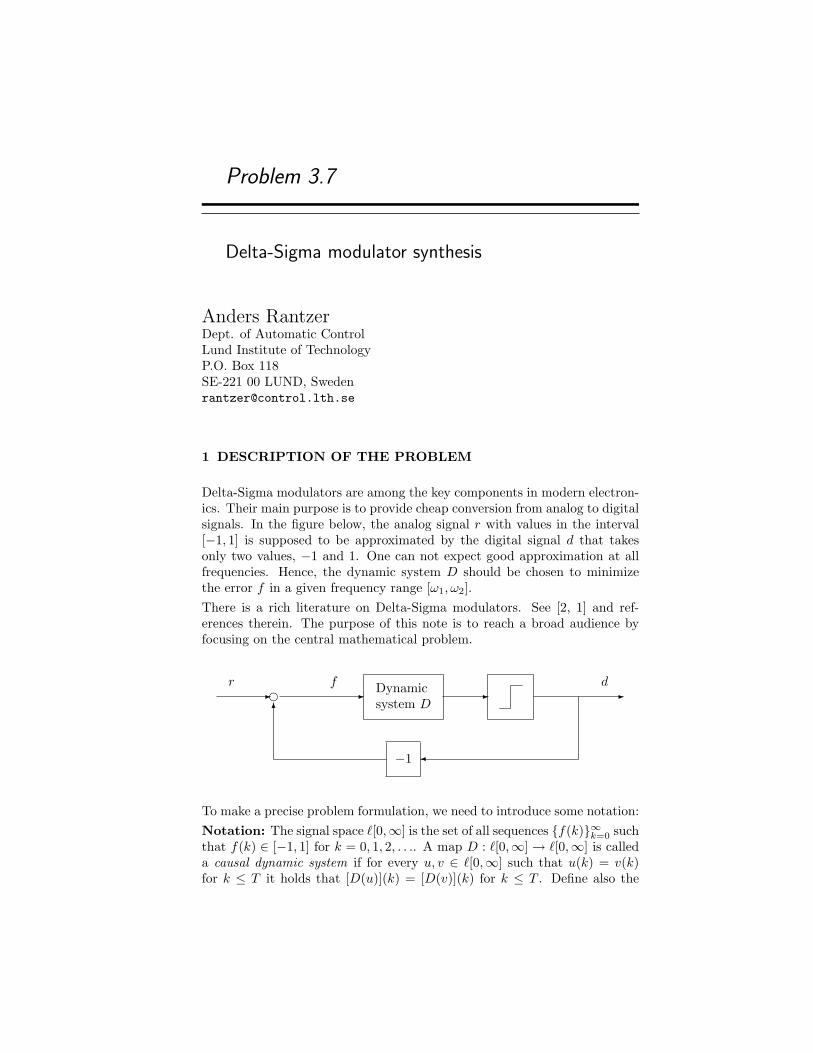
Problem 3.7
Delta-Sigma modulator synthesis
Anders RantzerDept. of Automatic ControlLund Institute of TechnologyP.O. Box 118SE-221 00 LUND, [email protected]
1 DESCRIPTION OF THE PROBLEM
Delta-Sigma modulators are among the key components in modern electron-ics. Their main purpose is to provide cheap conversion from analog to digitalsignals. In the figure below, the analog signal r with values in the interval[−1, 1] is supposed to be approximated by the digital signal d that takesonly two values, −1 and 1. One can not expect good approximation at allfrequencies. Hence, the dynamic system D should be chosen to minimizethe error f in a given frequency range [ω1, ω2].There is a rich literature on Delta-Sigma modulators. See [2, 1] and ref-erences therein. The purpose of this note is to reach a broad audience byfocusing on the central mathematical problem.
e Dynamicsystem D
-
−1
6
- --r f d
To make a precise problem formulation, we need to introduce some notation:Notation: The signal space `[0,∞] is the set of all sequences f(k)∞k=0 suchthat f(k) ∈ [−1, 1] for k = 0, 1, 2, . . .. A map D : `[0,∞] → `[0,∞] is calleda causal dynamic system if for every u, v ∈ `[0,∞] such that u(k) = v(k)for k ≤ T it holds that [D(u)](k) = [D(v)](k) for k ≤ T . Define also the
DELTA-SIGMA MODULATOR SYNTHESIS 115
function
sgn(x) =
1 if x ≥ 0−1 else
Problem: Given r ∈ `[0,∞] and a causal dynamic system D, define d, f ∈`[0,∞] by
d(k + 1) = sgn([D(f)](k)
), d(0) = 0
f(k) = r(k)− d(k)
and find a causal dynamic system D such that regardless of the referenceinput r, the error signal f becomes small in a prespecified frequency interval[ω1, ω2].The problem formulation is intentionally left vague on the last line. The sizeof f can be measured in many different ways. One option is to require auniform bound on
lim supT→∞
1T
∣∣∣∣∣T∑k=0
e−ikωf(k)
∣∣∣∣∣for all ω ∈ [ω1, ω2] and all reference signals r ∈ `[0,∞].Another option is to allow D to be stochastic system and put a bound onthe spectral density of f in the frequency interval. This would be consistentwith the wide-spread practice to add a stochastic “dithering signal” beforethe nonlinearity in order to avoid undesired periodic orbits.
2 AVAILABLE RESULTS
The simplest and best understood case is wherex(k + 1) = x(k) + f(k)f(k) = r(k)− sgn(x(k))
In this case, it is easy to see that the set x ∈ [−2, 2] is invariant, so with
FT (z) =T∑k=0
z−kf(k) XT (z) =T∑k=0
z−kx(k)
116 PROBLEM 3.7
it holds that1T
∫ ω0
0
|FT (eiω)|2dω =1T
∫ ω0
0
|(eiω − 1)XT (eiω)|2dω
=1T
∫ ω0
0
[2(1− cosω)|XT (eiω)|2
]dω
≤ 2(1− cosω0)1T
∫ π
0
|XT (eiω)|2dω
= 2(1− cosω0)π
T
T∑k=0
x(k)2
≤ 8π(1− cosω0)
which clearly bounds the error f at low frequencies.Many modifications using higher order dynamics have been suggested inorder to further reduce the error. However, there is still a strong demandfor improvements and a better understanding of the nonlinear dynamics.The following two references are suggested as entries to the literature on∆-Σ-modulators:
BIBLIOGRAPHY
[1] James A. Cherry, Continuous Time Delta-Sigma Modulators for High-Speed A/D Conversion: Theory, Practice & Fundamental PerformanceLimits, Kluwer, 1999.
[2] S. R. Norsworthy, R. Schreier, and G. C. Temes, Delta-Sigma Data Con-verters, IEEE Press, New York, 1997.
Problem 3.8
Determining of various asymptotics of solutions of
nonlinear time-optimal problems via right ideals in
the moment algebra
G. M. SklyarSzczecin UniversityWielkopolska str. 15, 70-451 Szczecin, Poland;Kharkov National UniversitySvoboda sqr. 4, 61077 [email protected], [email protected]
S. Yu. IgnatovichKharkov National UniversitySvoboda sqr. 4, 61077 Kharkov, [email protected]
1 MOTIVATION AND HISTORY OF THE PROBLEM
The time-optimal control problem is one of the most natural and at the sametime difficult problems in the optimal control theory.For linear systems, the maximum principle allows to indicate a class of opti-mal controls. However, the explicit form of the solution can be given only ina number of particular cases [1-3]. At the same time [4], an arbitrary lineartime-optimal problem with analytic coefficients can be approximated (in aneighborhood of the origin) by a certain linear problem of the form
xi = −tqiu, i = 1, . . . , n, q1 < · · · < qn, x(0) = x0, x(θ) = 0,
|u| ≤ 1, θ → min . (1)
In the nonlinear case, the careful analysis is required for any particularsystem [5, 6]. However, in a number of cases the time-optimal problem for anonlinear system can be approximated by a linear problem of the form (1)[7]. We recall this result briefly. Consider the time-optimal problem in the
118 PROBLEM 3.8
following statement
x = a(t, x) + ub(t, x), a(t, 0) ≡ 0, x(0) = x0, x(θ) = 0, |u| ≤ 1, θ → min,(2)
where a, b are real analytic in a neighborhood of the origin in Rn+1. Let usdenote by (θx0 , ux0) the solution of this problem.Denote by Ra, Rb the operators acting as Rad(t, x) = dt(t, x) + dx(t, x) ·a(t, x), Rbd(t, x) = dx(t, x) · b(t, x) for any vector function d(t, x) analyticin a neighborhood of the origin in Rn+1 and let ad m+1
RaRb = [Ra, admRa
Rb],m ≥ 0; ad 0
RaRb = Rb, where [·, ·] is the operator commutator. Denote
E(x) ≡ x.Theorem 1: The conditions rankadjRa
RbE(x)∣∣
t=0x=0
j≥0 = n and
[adm1RaRb, · · · [admk−1
RaRb, admk
RaRb] · · · ]E(x)
∣∣t=0x=0
∈ Lin
adjRaRbE(x)
∣∣t=0x=0
m−2
j=0
(3)for any k ≥ 2 and m1, . . . ,mk ≥ 0, where m = m1 + · · · + mk + k, hold ifand only if there exist a nonsingular transformation Φ of a neighborhood ofthe origin in Rn, Φ(0) = 0, and a linear time-optimal problem of the form(1), which approximates problem (2) in the following sense
θΦ(x0)
θLinx0
→ 1,1θ
∫ θ
0
|uLinx0 (t)− uΦ(x0)(t)|dt→ 0 as x0 → 0,
where (θLinx0 , uLinx0 ) denotes the solution of (1) and θ = minθΦ(x0), θLinx0 .
That means that if the conditions of theorem 1 are not satisfied, then theasymptotic behavior of the solution of the nonlinear time-optimal problemdiffers from asymptotics of solutions of all linear problems.In order to formulate the next result, let us give the representation of thesystem in the form of a series of nonlinear power moments [7]. We assumethe initial point x0 is steered to the origin in the time θ by the control u(t)w.r.t. system (2). Then under our assumptions for rather small θ one has
x0 =∞∑m=1
∑m1+···+mk+k=m
vm1...mkξm1...mk
(θ, u), (4)
where ξm1...mk(θ, u) =
∫ θ0
∫ τ10· · ·∫ τk−1
0
∏kj=1 τ
mj
j u(τj) dτk · · · dτ2dτ1 are non-linear power moments and
vm1...mk=
(−1)k
m1! · · ·mk!adm1RaRb adm2
RaRb · · · admk
RaRbE(x)
∣∣t=0x=0
.
We say that ord(ξm1...mk) = m1 + · · ·+mk + k is the order of ξm1...mk
.Theorem 1 means that there exists a transformation Φ which reduces (4) to
(Φ(x0))i = ξqi(θ, u) + ρi, i = 1, . . . , n,
where ρi includes power moments of order greater than qi+1 only while therepresentation (4) for the linear system (1) obviously has the form
x0i = ξqi
(θ, u), i = 1, . . . , n.
ASYMPTOTICS OF SOLUTIONS OF TIME-OPTIMAL PROBLEMS 119
That is the linear moments that correspond to the linear time-optimal prob-lem (1) form the principal part of the series in representation (4) as θ → 0.When condition (3) is not satisfied, one can try to find a nonlinear systemwhich has rather simply form and approximates system (2) in the sense oftime optimality. In [8] we claim the following result.Consider the linear span A of all nonlinear moments ξm1...mk
over R as afree algebra with the basis (ξm1...mk
: k ≥ 1,m1, . . . ,mk ≥ 0) and theproduct ξm1...mk
ξn1...ns= ξm1...mkn1...ns
. Introduce the inner product inA assuming the basis (ξm1...mk
) to be orthonormal. Consider also the Liealgebra L over R generated by the elements (ξm)∞m=0 with the commutator[`1, `2] = `1`2− `2`1. Introduce further the graded structure A =
∑∞m=1 Am
putting Am = Linξm1...mk: ord(ξm1...mk
) = m.Consider now a system of the form (2). The series in (4) naturally definesthe linear mapping v : A → Rn by the rule v(ξm1...mk
) = vm1...mk. Further
we assume the system (2) to be n-dimensional, i.e. dim v(L) = n. Notethat the form of coefficients vm1...mk
of the series in (4) implies the followingproperty of the mapping v: the equality v(`) = 0 for ` ∈ L implies v(`x) = 0for any x ∈ A. That means that any system of the form (2) generates a rightideal in the algebra A. We introduce the right ideal in the following way.Consider the sequence of subspaces Dr = v(L ∩ (A1 + · · ·+ Ar)) ⊂ Rn, andput r0 = minr : dimDr = n. For any r ≤ r0 consider a subspace Pr of allelements y ∈ L ∩ Ar such that v(y) ∈ Dr−1 (we assume D0 = 0). Thenput J =
∑r0r=1 Pr(A + R). Let J⊥ be the orthogonal complement of J . In
the next theorem LJ⊥ denotes the projection of the Lie algebra L on J⊥.Theorem 2: (A) Let system (2) be n-dimensional, ˜1, . . . , ˜n be a basis of∑r0r=1(LJ⊥ ∩ Ar) such that ord(˜i) ≤ ord(˜j) as i < j. Then there exists a
nonsingular analytic transformation Φ of a neighborhood of the origin thatreduces (4) to the following form
(Φ(x0))i = ˜i + ρi, i = 1, . . . , n,
where ρi contains moments of order greater than ord(˜i) only. Moreover,there exists a control system of the form
x = ub∗(t, x), (5)
such that representation (4) for this system is of the form
x0i = ˜
i, i = 1, . . . , n. (6)
(B) Suppose there exists an open domain Ω ⊂ Rn\0, 0 ∈ Ω, such thati) the time-optimal problem for system (5) with representation (6) has aunique solution (θ∗x0 , u∗x0(t)) for any x0 ∈ Ω;
ii) the function θ∗x0 is continuous for x0 ∈ Ω;
iii) denote K = u∗x0(tθ∗x0) : x0 ∈ Ω and suppose that the following con-dition holds: when considering K as a set in the space L2(0, 1), the weakconvergence of a sequence of elements fromK implies the strong convergence.

120 PROBLEM 3.8
Then the time-optimal problem for system (5) approximates problem (2) inthe domain Ω in the following sense: there exists a set of pairs (θx0 , ux0(t)),x0 ∈ Ω, such that the control ux0(t) steers the point Φ(x0) to the origin inthe time θx0 w.r.t. system (2) and
θΦ(x0)
θ∗x0
→ 1,θx0
θ∗x0
→ 1,1θ
∫ θ
0
|u∗x0(t)− ux0(t)|dt→ 0 as x0 → 0, x0 ∈ Ω,
where θΦ(x0) is the optimal time for problem (2) and θ = minθx0 , θ∗x0.Remark 1: If there exists the autonomous system x = a(x) + ub(x) suchthat its representation (4) is of the form (6) and the origin belongs to theinterior of the controllability set then the function θ∗x0 is continuous in aneighborhood of the origin [9]. Further, if time-optimal controls for system(5) are bang-bang then they satisfy condition iii) of theorem 2.Remark 2: Consider any r0 ≥ 0 and an arbitrary sequence of subspacesM = Mrr0r=1, Mr ⊂ L ∩Ar, such that
∑r0r=1(dim(L ∩Ar)− dimMr) = n.
Put JM =∑r0r=1Mr(A + R). We denote by J the set of all such ideals. For
any J ∈ J one can construct a control system of the form (5) such that itsrepresentation (4) is of the form (6).
2 FORMULATION OF THE PROBLEM.
Thus, the steering problem x = a(t, x)+ub(t, x), x(θ) = 0, where a(t, 0) ≡ 0,generates the right ideal in the algebra A, which defines system (5), and, un-der conditions i)–iii) of theorem 2, describes the asymptotics of the solutionof time-optimal problem (2). The question is: if any system of the form(5) having the representation of the form (6) satisfies conditions i)–iii) oftheorem 2. The positive answer means that all possible asymptotics of so-lutions of the time-optimal problems (2) are represented as asymptotics ofsolutions of the time-optimal problems for systems (5) with representationsof the form (6).In other words, if any system of the form (5) having the representation of theform (6) satisfies conditions i)–iii) of theorem 2, then time-optimal problems(2) induce the same structure in the algebra A as steering problems to theorigin under the constraint |u| ≤ 1, namely, the set of right ideals J. If thisis not the case, then the next problem is to describe constructively the classof such systems.
BIBLIOGRAPHY
[1] V. I. Korobov and G. M. Sklyar, “Time optimality and the power momentproblem,” Math. USSR Sb., 62, pp. 185-205,1989.
ASYMPTOTICS OF SOLUTIONS OF TIME-OPTIMAL PROBLEMS 121
[2] V. I. Korobov and G. M. Sklyar, “Time optimality and the trigonometricmoment problem,” Math. USSR Izv., 35, pp. 203-220,1990.
[3] V. I. Korobov and G. M. Sklyar, “Markov power min-problem with pe-riodic gaps,” J. Math. Sci., 80 , pp. 1559-1581, 1996.
[4] G. M. Sklyar and S. Yu. Ignatovich, “A classification of linear time-optimal control problems in a neighborhood of the origin,” J. Math.Anal. Applic., 203, pp. 791-811, 1996.
[5] A. Bressan, “The generic local time-optimal stabilizing controls in di-mension 3,” SIAM J. Control Optimiz., 24, pp. 177-190, 1986.
[6] B. Bonnard, “On singular estremals in the time minimal control problemin R3,” SIAM J. Control Optimiz., 23, pp. 794-80, 1985.
[7] G. M. Sklyar and S. Yu. Ignatovich, “Moment approach to nonlineartime optimality,” SIAM J. Control Optimiz., 38, pp. 1707-1728, 2000.
[8] G. M. Sklyar and S. Yu. Ignatovich, “Approximation in the sense of timeoptimality via nonlinear moment problems,” SIAM J. Control Optimiz.
[9] V. I. Korobov, “On continuous dependence of the solution of the opti-mal control problem with free time on initial data,” Differen. Uravn., 7,pp. 1120-1123, 1971, (in Russian).
Problem 3.9
Dynamics of principal and minor component flows
U. Helmke and S. YoshizawaDepartment of MathematicsUniversity of WurzburgAm Hubland, D-97074 [email protected]
R. Evans, J.H. Manton and I.M.Y. MareelsDepartment of Electrical and Electronic EngineeringThe University of MelbourneVictoria [email protected]
Stochastic subspace tracking algorithms in signal processing and neural net-works are often analyzed by studying the associated matrix differential equa-tions. Such gradient-like nonlinear differential equations have an intricateconvergence behavior that is reminiscent of matrix Riccati equations. Infact, these types of systems are closely related. We describe a number ofopen research problems concerning the dynamics of such flows for principaland minor component analysis.
1 DESCRIPTION OF THE PROBLEM
Principal component analysis is a widely used method in neural networks,signal processing, and statistics for extracting the dominant eigenvalues ofthe covariance matrix of a sequence of random vectors. In the literature, var-ious algorithms for principal component and principal subspace analysis havebeen proposed along with some, but in many aspects incomplete, theoreticalanalyzes of them. The analysis is usually based on stochastic approximationtechniques and commonly proceeds via the so-called Ordinary DifferentialEquation (ODE) method, i.e., by associating an ODE whose convergenceproperties reflect that of the stochastic algorithm; see e.g., [7]. In the sequel,we consider some of the relevant ODEs in more detail and pose some open
DYNAMICS OF PRINCIPAL AND MINOR COMPONENT FLOWS 123
problems concerning the dynamics of the flows.In order to state our problems in precise mathematical terms, we give aformal definition of a principal and minor component flow.Definition[PSA/MSA Flow]:A normalized subspace flow for a covariancematrix C is a matrix differential equation X = f(X) on Rn×p with thefollowing properties:
1. Solutions X(t) exist for all t ≥ 0 and have constant rank.
2. If X0 is orthonormal, then X(t) is orthornormal for all t.
3. limt→∞X(t) = X∞ exists for all full rank initial conditions X0.
4. X∞ is an orthonormal basis matrix of a p-dimensional eigenspace ofC.
The subspace flow is called a PSA (principal subspace) or MSA (minor sub-space) flow, if, for generic initial conditions, the solutions X(t) converge fort→∞ to an orthonormal basis of the eigenspace that is spanned by the firstp dominant or minor eigenvectors of C, respectively.In the neural network and signal processing literature, a number of suchprincipal subspace flows have been considered. The best-known example ofa PSA flow is Oja’s flow [9, 10]
X = (I −XX ′)CX. (1)
Here C = C ′ > 0 is the n× n covariance matrix and X is an n× p matrix.Actually, it is nontrivial to prove that this cubic matrix differential equationis indeed a PSA in the above sense and thus, generically, converges to adominant eigenspace basis. Another, more general example of a PSA flow isthat introduced by [12, 13] and [17]:
X = CXN −XNX ′CX (2)
Here N = N ′ > 0 denotes an arbitrary diagonal k × k matrix with distincteigenvalues. This system is actually a joint generalization of Oja’s flow (1)and of Brockett’s [1] gradient flow on orthogonal matrices
X = [C,XNX ′]X (3)
For symmetric matrix diagonalisation, see also [6]. In [19], Oja’s flow wasre-derived by first proposing the gradient flow
X = (C(I −XX ′) + (I −XX ′)C)X (4)
and then omitting the first term C(I − XX ′)X because C(I − XX ′)X =CX(I − X ′X) → 0, a consequence of both terms in (4) forcing X to theinvariant manifold X : X ′X = I. Interestingly, it has recently been real-ized [8] that (4) has certain computational advantages compared with (1),however, a rigorous convergence theory is missing. Of course, these threesystems are just prominent examples from a bigger list of potential PSA
124 PROBLEM 3.9
flows. One open problem in most of the current research is a lack of a fullconvergence theory, establishing pointwise convergence to the equilibria. Inparticular, a solution to the following three problems would be highly desir-able. The first problem addresses the qualitative analysis of the flows.
Problem 1. Develop a complete phase portrait analysis of (1), (2) and (4).In particular, prove that the flows are PSA, determine the equilibria points,their local stability properties and the stable and unstable manifolds for theequilibrium points.The previous systems are useful for principal component analysis, but theycannot be used immediately for minor component analysis. Of course, onepossible approach might be to apply any of the above flows with C replacedby C−1. Often this is not reasonable though, as in most applications thecovariance matrix C is implemented by recursive estimates and one doesnot want to invert these recursive estimates on line. Another alternativecould be to put a negative sign in front of the equations. But this does notwork either, as the minor component equilibrium point remains unstable.In the literature, therefore, other approaches to minor component analysishave been proposed [2, 3, 5], but without a complete convergence theory.1
Moreover, a guiding geometric principle that allows for the systematic con-struction of minor component flows is missing. The key idea here seems tobe an appropriate concept of duality between principal and minor compo-nent analysis.
Conjecture 1. Principal component flows are dual to minor componentflows, via an involution in matrix space Rn×p, that establishes a bijectivecorrespondence between solutions of PSA flows and MSA flows, respectively.If a PSA flow is actually a gradient flow for a cost function f , as is the casefor (1), (2) and (4), then the corresponding dual MSA flow is a gradient flowfor the Legendre dual cost function f∗ of f .When implementing these differential equations on a computer, suitable dis-cretizations are to be found. Since we are working in unconstrained Eu-clidean matrix space Rn×p, we consider Euler step discretizations. Thus,e.g., for system (1) consider
Xt+1 = Xt − st(I −XtX′t)CXt, (5)
with suitably small step sizes. Such Euler discretization schemes are widelyused in the literature, but usually without explicit step-size selections thatguarantee, for generic initial conditions, convergence to the p dominant or-thonormal eigenvectors of A. A further challenge is to obtain step-size se-lections that achieve quadratic convergence rates (e.g., via a Newton-typeapproach).
1It is remarked that the convergence proof in [5] appears flawed; they argue that
because d vec Qdt
= G(t) vec Q for some matrix G(t) < 0 then Q → 0. However, counter-examples are known [15] where G(t) is strictly negative definite (with constant eigenvalues)yet Q diverges.

DYNAMICS OF PRINCIPAL AND MINOR COMPONENT FLOWS 125
Problem 2. Develop a systematic convergence theory for discretisations ofthe flows, by specifying step-size selections that imply global as well as localquadratic convergence to the equilibria.
2 MOTIVATION AND HISTORY
Eigenvalue computations are ubiquitous in Mathematics and EngineeringSciences. In applications, the matrices whose eigenvectors are to be foundare often defined in a recursive way, thus demanding recursive computa-tional methods for eigendecomposition. Subspace tracking algorithms arewidely used in neural networks, regression analysis, and signal processingapplications for this purpose. Subspace tracking algorithms can be studiedby replacing the stochastic, recursive algorithm through an averaging proce-dure by a nonlinear ordinary differential equation. Similarly, new subspacetracking algorithms can be developed by starting with a suitable ordinary dif-ferential equation and then converting it to a stochastic approximation algo-rithm [7]. Therefore, understanding the dynamics of such flows is paramountto the continuing development of recursive eigendecomposition techniques.The starting point for most of the current work in principal componentanalysis and subspace tracking has been Oja’s system from neural networktheory. Using a simple Hebbian law for a single perceptron with a linearactivation function, Oja [9, 10] proposed to update the weights according to
Xt+1 = Xt − st(I −XtX′t)utu
′tXt. (6)
Here Xt denotes the n × p weight matrix and ut the input vector of theperceptron, respectively. By applying the ODE method to this system, Ojaarrives at the differential equation (1). Here C = E(utu′t) is the covariancematrix. Similarly, the other flows, (2) and (4), have analogous interpreta-tions.In [9, 11] it is shown for p = 1 that (1) is a PSA flow, i.e., it converges forgeneric initial conditions to a normalised dominant eigenvector of C. In [11]the system (1) was studied for arbitrary values of p and it was conjecturedthat (1) is a PSA flow. This conjecture was first proven in [18], assumingpositive definiteness of C. Moreover, in [18, 4], explicit initial conditions interms of intersection dimensions for the dominant eigenspace with the initalsubspace were given, such that the flow converges to a basis matrix of thep-dimensional dominant eigenspace. This is reminiscent of Schubert typeconditions in Grassmann manifolds.Although the Oja flow serves as a principal subspace method, it is not usefulfor principal component analysis because it does not converge in general toa basis of eigenvectors. Flows for principal component analysis such as (2)have been first studied in [14, 12, 13, 17]. However, pointwise convergence tothe equilibria points was not established. In [16] a Lyapunov function for theOja flow (1) was given, but without recognizing that (1) is actually a gradient

126 PROBLEM 3.9
flow. There have been confusing remarks in the literature claiming that (1)cannot be a gradient system as the linearization is not a symmetric matrix.However, this is due to a misunderstanding of the concept of a gradient.In [20] it is shown that (2), and in particular (1), is actually a gradient flow forthe cost function f(X) = 1/4tr(AXNX ′)2−1/2tr(A2XD2X ′) and a suitableRiemannian metric on Rn×p. Moreover, starting from any initial conditionin Rn×p, pointwise convergence of the solutions to a basis of k independenteigenvectors of A is shown together with a complete phase portrait analysisof the flow. First steps toward a phase portrait analysis of (4) are madein [8].
3 AVAILABLE RESULTS
In [12, 13, 17] the equilibrium points of (2) were computed together with alocal stability analysis. Pointwise convergence of the system to the equilibriais established in [20] using an early result by Lojasiewicz on real analyticgradient flows. Thus these results together imply that (2), and hence (1), isa PSA. An analogous result for (4) is forthcoming; see [8] for first steps inthis direction. Sufficient conditions for initial matrices in the Oja flow (1) toconverge to a dominant subspace basis are given in [18, 4], but not for theother, unstable equilibria, nor for system (2). A complete characterizationof the stable/unstable manifolds is currently unknown.
BIBLIOGRAPHY
[1] R. W. Brockett, “Dynamical systems that sort lists, diagonalise ma-trices, and solve linear programming problems,” Linear Algebra Appl.,146:79–91, 1991.
[2] T. Chen, “ Modified Oja’s algorithms for principal subspace and minorsubspace extraction,” Neural Processing Letters, 5:105–110, April 1997.
[3] T. Chen, S. Amari, and Q. Lin, “ A unified algorithm for principal andminor component extraction,” Neural Networks, 11:385–390, 1998.
[4] T. Chen, Y. Hua, and W.-Y. Yan, “Global convergence of Oja’s sub-space algorithm for principal component extraction,” IEEE Transac-tions on Neural Networks, 9(1):58–67, 1998.
[5] S. C. Douglas, S.-Y. Kung, and S. Amari, “A self-stabilized minor sub-space rule,” IEEE Signal Processing Letters, 5(12):328–330, December1998.
[6] U. Helmke and J. B. Moore, Optimization and Dynamical Systems,Springer-Verlag, 1994.
DYNAMICS OF PRINCIPAL AND MINOR COMPONENT FLOWS 127
[7] H. J. Kushner and G. G. Yin, Stochastic Approximation Algorithms andApplications, Springer, 1997.
[8] J. H. Manton, I. M. Y. Mareels, and S. Attallah, “An analysis of the fastsubspace tracking algorithm NOja,” In: IEEE Conference on Acoustics,Speech and Signal Processing, Orlando, Florida, May 2002.
[9] E. Oja, “A simplified neuron model as a principal component analyzer,”Journal of Mathematical Biology, 15:267–273, 1982.
[10] E. Oja, “ Neural networks, principal components, and subspaces,” In-ternational Journal of Neural Systems, 1:61–68, 1989.
[11] E. Oja and J. Karhunen, “On stochastic approximation of the eigenvec-tors and eigenvalues of the expectation of a random matrix,” Journalof Mathematical Analysis and Applications, 106:69–84, 1985.
[12] E. Oja, H. Ogawa, and J. Wangviwattana, “Principal component anal-ysis by homogeneous neural networks, Part I: The weighted subspacecriterion,” IEICE Transactions on Information and Systems, 3:366–375,1992.
[13] E. Oja, H. Ogawa, and J. Wangviwattana, “Principal component anal-ysis by homogeneous neural networks, Part II: Analysis and extensionsof the learning algorithms,” IEICE Transactions on Information andSystems, 3:376–382, 1992.
[14] T. D. Sanger, “Optimal unsupervised learning in a single-layer linearfeedforward network,” Neural Networks, 2:459–473, 1989.
[15] J. L. Willems, Stability Theory of Dynamical Systems, Studies in Dy-namical Systems, London, Nelson, 1970.
[16] J. L. Wyatt and I. M. Elfadel, “Time-domain solutions of Oja’s equa-tions,” Neural Computation, 7:915–922, 1995.
[17] L. Xu, “Least mean square error recognition principle for self organizingneural nets,” Neural Networks, 6:627–648, 1993.
[18] W.-Y. Yan, U. Helmke, and J. B. Moore, “Global analysis of Oja’s flowfor neural networks,” IEEE Transactions on Neural Networks, 5(5):674–683, September 1994.
[19] B. Yang, “Projection approximation subspace tracking”, IEEE Trans-actions on Signal Processing, 43(1):95–107, January 1995.
[20] S. Yoshizawa, U. Helmke, and K. Starkov, “Convergence analysis forprincipal component flows,” International Journal of Applied Mathe-matics and Computer Science, 11:223–236, 2001.


PART 4
Discrete Event, Hybrid Systems

Problem 4.1
L2-induced gains of switched linear systems
Joao P. Hespanha1
Dept. of Electrical and Computer EngineeringUniversity of California, Santa [email protected]
1 SWITCHED LINEAR SYSTEMS
In the 1999 collection of Open Problems in Mathematical Systems and Con-trol Theory, we proposed the problem of computing input-output gains ofswitched linear systems. Recent developments provided new insights intothis problem leading to new questions.
A switched linear system is defined by a parameterized family of realizations(Ap, Bp, Cp, Dp) : p ∈ P, together with a family of piecewise constantswitching signals S := σ : [0,∞) → P. Here we consider switched sys-tems for which all the matrices Ap, p ∈ P are Hurwitz. The correspondingswitched system is represented by
x = Aσx+Bσu, y = Cσx+Dσu, σ ∈ S (1)and by a solution to (1), we mean a pair (x, σ) for which σ ∈ S and x is asolution to the time-varying system
x = Aσ(t)x+Bσ(t)u, y = Cσ(t)x+Dσ(t)u, t ≥ 0. (2)Given a set of switching signals S, we define the L2-induced gain of (1) by
infγ ≥ 0 : ‖y‖2 ≤ γ‖u‖2, ∀u ∈ L2, x(0) = 0, σ ∈ S,where y is computed along solutions to (1). The L2-induced gain of (1)can be viewed as a “worst case” energy amplification gain for the switchedsystem, over all possible inputs and switching signals and is an importanttool to study the performance of switched systems, as well as the stabilityof interconnections of switched systems.
1This material is based upon work supported by the National Science Foundation underGrant No. ECS-0093762.

132 PROBLEM 4.1
2 PROBLEM DESCRIPTION
We are interested here in families of switching signals for which consecutivediscontinuities are separated by no less than a positive constant called thedwell-time. For a given τD > 0, we denote by S[τD] the set of piecewiseconstant switching signals with interval between consecutive discontinuitiesno smaller than τD. The general problem that we propose is the computationof the function g : [0,∞) → [0,∞] that maps each dwell-time τD with theL2-induced gain of (1), for the set of dwell-time switching signals S := S[τD].Until recently? little more was known about g other than the following:
1. g is monotone decreasing
2. g is bounded below by
gstatic := supp∈P
‖Cp(sI −Ap)−1Bp +Dp‖∞,
where ‖T‖∞ := sup<[s]≥0 ‖T (s)‖ denotes the H∞-norm of a transfermatrix T . We recall that ‖T‖∞ is numerically equal to the L2-inducedgain of any linear time-invariant system with transfer matrix T .
Item 1 is a trivial consequence of the fact that given two dwell-times τD1 ≤τD2 , we have that S[τD1 ] ⊃ S[τD2 ]. Item 2 is a consequence of the fact thatevery set S[τD], τD > 0 contains all the constant switching signals σ = p,p ∈ P. It was shown in [2] that the lower-bound gstatic is strict and in generalthere is a gap between gstatic and
gslow := limτD→∞
g[τD].
This means that even switching arbitrarily seldom, one may not be able torecover the L2-induced gains of the “unswitched systems.” In [2] a procedurewas given to compute gslow. Opposite to what had been conjectured, gslow
is realization dependent and cannot be determined just from the transferfunctions of the systems being switched.
The function g thus looks roughly like the ones shown in figure 4.1.1, where(a) corresponds to a set of realizations that remains stable for arbitrarily fastswitching and (b) to a set that can exhibit unstable behavior for sufficientlyfast switching [3]. In (b), the scalar τmin denotes the smallest dwell-time forwhich instability can occur for some switching signal in S[τmin].
Several important basic questions remain open:
1. Under what conditions is g bounded? This is really a stability problemwhose general solution has been eluding researchers for a while now (cf.,the survey paper [3] and references therein).
2. In case g is unbounded (case (b) in figure 4.1.1), how to computethe position of the vertical asymptote? Or, equivalently, what is thesmallest dwell-time τmin for which one can have instability?
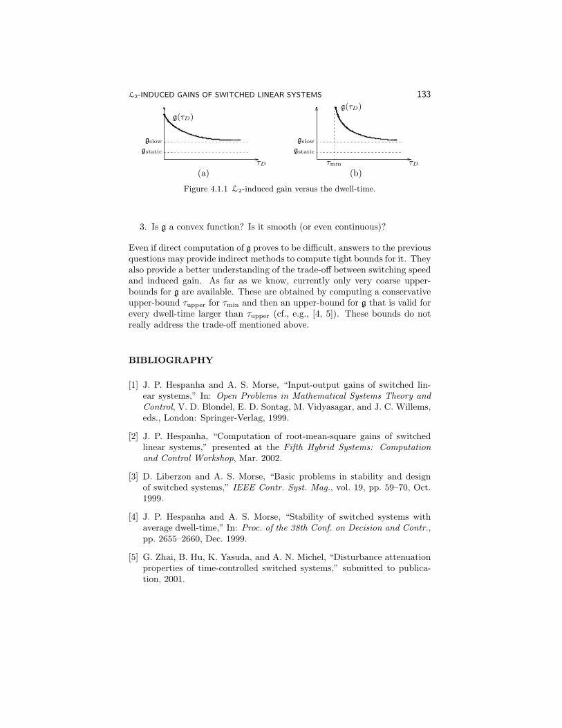
L2-INDUCED GAINS OF SWITCHED LINEAR SYSTEMS 133
gstatic
gslow
τD
g(τD)
gstatic
gslow
g(τD)
τDτmin
(a) (b)
Figure 4.1.1 L2-induced gain versus the dwell-time.
3. Is g a convex function? Is it smooth (or even continuous)?
Even if direct computation of g proves to be difficult, answers to the previousquestions may provide indirect methods to compute tight bounds for it. Theyalso provide a better understanding of the trade-off between switching speedand induced gain. As far as we know, currently only very coarse upper-bounds for g are available. These are obtained by computing a conservativeupper-bound τupper for τmin and then an upper-bound for g that is valid forevery dwell-time larger than τupper (cf., e.g., [4, 5]). These bounds do notreally address the trade-off mentioned above.
BIBLIOGRAPHY
[1] J. P. Hespanha and A. S. Morse, “Input-output gains of switched lin-ear systems,” In: Open Problems in Mathematical Systems Theory andControl, V. D. Blondel, E. D. Sontag, M. Vidyasagar, and J. C. Willems,eds., London: Springer-Verlag, 1999.
[2] J. P. Hespanha, “Computation of root-mean-square gains of switchedlinear systems,” presented at the Fifth Hybrid Systems: Computationand Control Workshop, Mar. 2002.
[3] D. Liberzon and A. S. Morse, “Basic problems in stability and designof switched systems,” IEEE Contr. Syst. Mag., vol. 19, pp. 59–70, Oct.1999.
[4] J. P. Hespanha and A. S. Morse, “Stability of switched systems withaverage dwell-time,” In: Proc. of the 38th Conf. on Decision and Contr.,pp. 2655–2660, Dec. 1999.
[5] G. Zhai, B. Hu, K. Yasuda, and A. N. Michel, “Disturbance attenuationproperties of time-controlled switched systems,” submitted to publica-tion, 2001.
Problem 4.2
The state partitioning problem of quantised systems
Jan LunzeInstitute of Automation and Computer ControlRuhr-University BochumD-44780 [email protected]
1 DESCRIPTION OF THE PROBLEM
Consider a continuous system whose state can only be accessed through aquantizer. The quantizer is defined by a partition of the state space. Thesystem generates an event if the system trajectory crosses the boundarybetween adjacent partitions.The problem concerns the prediction of the event sequence generated by thesystem for a given initial event. As the initial event does not define theinitial system state unambiguously but only restricts the initial state to apartition boundary, when predicting the system behavior the bundle of allstate trajectories have to be considered that start on this partition boundary.The question to be answered is: under what conditions on the vector fieldof the system and the state partition is the event sequence unique?In more detail, consider the continuous-variable system
x= f(x(t)), x(0) = x0 (1)
with the state x ∈ X ⊆ Rn. The vector field f satisfies a Lipschitz conditionso that eqn. (1) has, for all x0 ∈ X, a unique solution.The state space X is partitioned into N disjoint sets Qx(i) (i = 1, 2, ..., N)that satisfy the conditions
X =N⋃i=1
Qx(i) and Qx(i) ∩ Qx(j) = ∅ for i 6= j.
The set
Q = Qx(i) : i = 1, 2, ..., N
THE STATE PARTITIONING PROBLEM OF QUANTISED SYSTEMS 135
is called a state quantization. The quantized state is denoted by [x] anddefined by
[x] = i ⇔ x ∈ Qx(i). (2)
The change of the quantized state is called an event, where the event eijoccurs at time t if the relations
[x(t+ δt)] = i and [x(t− δt)] = j
hold for small δt > 0. Hence, at time t the state x is on the boundarybetween the state partitions Qx(i) and Qx(j)
x(t) ∈ δQx(i) ∩ Qx(j),
where δQx denotes the hull of Qx. The system (1) together with the quan-tization Q is called the quantized system.For given initial state x0 the system (1) generates, for the time interval [0, T ],a unique state trajectory x(x0, t) and, hence, a unique event sequence
E = (e0, e1, ..., eH) = Quant(x(x0, t)),
which formally can be represented as the result of the operator Quant appliedto the state trajectory. H is the number of events generated by the systemwithin the time interval [0, T ]. The following considerations concern onlythose initial events e0 for which the quantized system generates an eventsequence with H > 1.If instead of the initial state x0 only the initial event e0 = eij is given, theinitial state is only known to lie on the boundary δQx(i)∩Qx(j) between thestate partitions Qx(i) and Qx(j). Consequently, the bundle of trajectoriesstarting in all these initial states have to be considered. These trajectoriesyield the set
E(e0) = E = Quant(x(x0, t)) for x0 ∈ δQx(i) ∩ Qx(j)of event sequences. If the set E has more than one element, the quantizedsystem is nondeterministic in the sense that the knowledge of the initial evente0 is not sufficient to predict the future event sequence unambiguously. Onthe other hand, the quantized system is called to be deterministic if the setE(e0) is a singleton for all possible initial events e0.
In order to define the events precisely, the state partition should satisfy thefollowing assumptions:A1. The trajectories do not lie in the hypersurfaces that represent the par-tition boundaries.A2. The system cannot generate an infinite number of events in a finitetime interval.A3. No fix-point of the vector field f lie on a partition boundary.
These assumptions can be satisfied by appropriately defining the state par-titions for the given vector field f .
136 PROBLEM 4.2
State partitioning problem. Find conditions under which thequantised system is deterministic.
This problem can be reformulated in two versions:
Problem: For given vector field f , find a partition of the statespace such that the quantized system is deterministic.
Problem B: For given vector field f and a state quantization Q,test whether the quantized system is deterministic.
Both formulations have their engineering relevance. Where problem A con-cerns the practical situation in which a state partition has to be selected,problem B refers to the test of the determinism of the system for givenpartition.The problem stated so far is, possibly, too general in two respects. First,the problem for testing the determinism of the system should be as simpleas possible. For a given partition consisting of N disjoint sets, Problem Bcan be solved by considering all trajectory bundles that start on all partitionboundaries. Here, the characterization of classes of vector fields f and parti-tioning methods is interesting for which the complexity of the test is constantor grows only linearly with N . Second, for problem A it is interesting to findpartitions that can be distinguished with only a few measurements. Forexample, rectangular partitions are interesting from a practical viewpointwhich result from separate quantizations of all n state variables xi.
Nonautonomous systems.The problem can be extended to nonautonomous quantized systems
x= f(x(t),u(t)), x(0) = x0 (3)y(t) =g(x(t),u(t)) (4)
with input u ∈ U ⊆ Rm and output y ∈ Y ⊆ Rr. The functions f andg satisfy a Lipschitz condition so that eqns. (3), (4) have, for all x0 ∈ X
and u(t), a unique solution. The output quantizer is defined by a partitionof the output space Y into the sets Qy(i) where the quantized output [y] isdefined analogously to equation (2). The event sequence E is now definedin terms of the events that the output signal y generates. The system isconsidered with the quantized input [u]. An injector associates with eachinput a unique element of the finite discrete set
U = u1,u2, ...,uM
such that u(t) = ui if [u(t)] = i. Again, a change of the quantized input valueis called an (input) event. It is assumed that the input and output eventsoccur synchronously. This assumption fixes the time instances in whichthe input changes its value. It is motivated by the fact that in closed-loop
THE STATE PARTITIONING PROBLEM OF QUANTISED SYSTEMS 137
systems a supervisor defines the quantized input in the same time instant inwhich an output event occurs.Here the state partitioning problem includes also to define an output parti-tion and an input set U such that the quantized system is deterministic forall input sequences.
2 MOTIVATION AND HISTORY OF THE PROBLEM
The problem results from hybrid systems, whose simplest form is a conti-nuous-variable system with discrete inputs. Many technological systems thatare controlled by programmable logic controllers (PLC) have a continuousstate space and are controlled by discrete inputs. The contrast of the conti-nous state and the discrete input does not matter because many systems aredesigned in such a way that any accessible input results in an unambiguousstate or output event.For example, the (simplified) state space of a lift has the state variables“vehicle position,” and “door position” both of which are quantized wherethe vehicle position refers to the floor in which it stops and the two discretedoor position are called “open” or “closed.” For the performance of thissystem, only the events are important, which refer to the beginning and theend of the presence of the vehicle or the door in one of these positions. Asthe PLC can only switch on or off, the motors of the vehicle or the doorand it is programmed so that the next command is given only after the nextoutput event has occurred, every new input event is followed by exactly oneoutput event (unless the system is faulty). So, the lift is a continuous-variablesystem (3), (4) with quantized input and output, that is deterministic.In this case, the solution to the state partitioning problem is simple. Thedeterminism of the quantized system results from the fact that the systemtrajectories are parallel to the coordinate axes of the state space for allaccessible inputs and the quantization refers to separate intervals of bothstate variables. So, the end point of any movement initiated by a PLCcommand is a point in the state space and every trajectory of the closed-loop system results in precisely one output event.In a more general setting, continuous-variable systems are dealt with asquantized systems for process supervision tasks. Then the system is notdesigned to behave like a discrete-event system but has a continuous statespace. The quantizers are introduced deliberately to reduce the informationto be processed. For example, alarm messages show that a certain signal hasexceeded a threshold. The state partitioning problem asks for the a choiceof discrete sensors such that the system behavior is deterministic.As the third motivation for the state partitioning problem, hybrid systemstheory concerns dynamical systems with continuous-variable and discrete-event subsystems. The interfaces between both parts are the quantizer and
138 PROBLEM 4.2
the injector introduced above that transform the discrete output signal ofthe discrete subsystem into a real-valued input signal of the continuous sub-system and vice versa. The problem occurs under what condition the overallhybrid system has a deterministic input-output behavior if only the discreteinputs and outputs of the discrete subsystem are considered. The mainsource of nondeterminism results from the quantization of the signal spaceof the continuous subsystem, which again leads to the state partitioningproblem.In all these situations, the discrete behavior of a continuous system is consid-ered. In the literature on fault diagnosis and verification of discrete controlalgorithms the hybrid nature of the closed-loop system is removed by using adiscrete-event representation of the quantized system. As in many practicalsituations the quantizers can be chosen, the state partitioning problem asksfor guidelines of this selection. For a deterministic discrete behavior, a de-terministic model can be used to describe the quantised system. If, however,the discrete behavior is non-deterministic, a nondeterministic model like anondeterministic or stochastic automaton or a Petri net has to be used.Several ways for determining such models for a given quantized system havebeen elaborated recently ([3], [4], [6], [7], [8], [9]).
3 AVAILABLE RESULTS
The first result on the state partitioning problem concerns discrete-timesystems (rather than continuous-time systems) with quantized state space.Reference [4] gives a necessary and sufficient condition for the determinismof the discrete behavior for linear autonomous systems with a state spacepartition that regularly decomposes each state variable into intervals of thesame size. In [5] it has been shown how state partitions can be generated bymapping a given initial set Qx(1) by the model (1) that is used with reversedtime axis.For the problem stated here, only preliminary results are available. If thesystem trajectories are, like in the lift example, parallel to the coordinateaxes of the state space and the quantization boundaries define rectangularcells whose axes are parallel to the coordinate axes, the discrete behavioris deterministic. This situation is encountered if, for example, the statevariables are decoupled and controlled by separate inputs. Hence, the modelcan be decomposed into
xi = fi(xi, ui)yi = gi(xi),
which corresponds again to the simple lift example. Another example is anundamped oscillator with a state partition that decomposes the state spaceinto the two half-planes. Then the fix-point lies on the partition boundary(and, thus, violates assumption A3). However, the oscillator generates, for
THE STATE PARTITIONING PROBLEM OF QUANTISED SYSTEMS 139
each initial state, a unique (alternating) event sequence.Results on symbolic dynamics are closely related to the problem stated here(cf. [1], [2]). A bundle of trajectories (or flows) is considered, which generatea symbolic output if some partition boundary is crossed. The partition iscalled Markovian if all trajectories of the bundle cross the same partitionboundary and, hence, generate the same symbol. In the terminology usedthere, the problem posed here asks the question how to find Markovianpartitions.
BIBLIOGRAPHY
[1] A. Lasota, M. C. Mackey, Chaos, Fractals and Noise, Springer-Verlag,New York, 1994.
[2] D. Lind, B. Marcus, An Introduction to Symbolic Dynamics and Coding,Cambridge University Press, 1995.
[3] J. Lunze, “A Petri net approach to qualitative modelling of continuousdynamical systems,” Systems Analysis, Modelling, Simulation, 9, pp.885-903, 1992.
[4] J. Lunze, “Qualitative modelling of linear dynamical systems with quan-tized state measurements,” Automatica, 30, pp. 417-431, 1994.
[5] J. Lunze, B. Nixdorf, J. Schroder, “On the nondeterminism of discrete-event representations of continuous-variables systems,” Automatica, 35,pp. 395-408, 1999.
[6] H.A. Preisig, M.J.H. Pijpers, M. Weiss, “A discrete modelling procedurefor continuous processes based on state-discretisation,” 2n MATHMOD,Vienna, pp. 189-194, 1997.
[7] J. Raisch, S. O’Young, “A totally ordered set of discrete abstractions fora given hybrid or continuous system,” pp. 342-360 In: P. Antsaklis, W.Kohn, A. Nerode, S. Sastry, eds., Hybrid Systems II, Springer-Verlag,Berlin, 1995.
[8] J. Schroder, Modelling, State Observation and Diagnosis of QuantisedSystems, Springer-Verlag, Heidelberg, 2002.
[9] O. Stursberg, S. Kowalewski, S. Engell, “Generating timed discretemodels,” 2n MATHMOD, Vienna, pp. 203-207, 1997.
Problem 4.3
Feedback control in flowshops
S. P. SethiSchool of ManagementThe University of Texas at DallasBox 830688, Mail Station JO4.7Richardson, TX [email protected]
Q. ZhangDepartment of MathematicsUniversity of GeorgiaAthens, GA [email protected]
1 DESCRIPTION OF THE PROBLEM
Consider a manufacturing system producing a single finished product usingm machines in tandem that are subject to breakdown and repair. We aregiven a finite-state Markov chain α(·) = (α1(·), . . . , αm(·)) on a probabilityspace (Ω,F, P ), where αi(t), i = 1, . . . ,m, is the capacity of the i-th machineat time t. We use ui(t) to denote the input rate to the i-th machine, i =1, . . . ,m, and xi(t) to denote the number of parts in the buffer between thei-th and (i+1)-th machines, i = 1, . . . ,m−1. Finally, the surplus is denotedby xm(t). The dynamics of the system can then be written as follows:
x(t) = Au(t) +Bz, x(0) = x, (1)
where z is the rate of demand and
A =
1 −1 0 · · · 00 1 −1 · · · 0...
...... · · ·
...0 0 0 · · · 1
and B =
00...
−1
.
FEEDBACK CONTROL IN FLOWSHOPS 141
Since the number of parts in the internal buffers cannot be negative, weimpose the state constraints xi(t) ≥ 0, i = 1, . . . ,m − 1. To formulate theproblem precisely, let S = [0,∞)m−1 × (−∞,∞) ⊂ Rm denote the stateconstraint domain. For α = (α1, . . . , αm) ≥ 0, let
U(α) = u = (u1, . . . , um) : 0 ≤ ui ≤ αi, i = 1, . . . ,m,
and for x ∈ S, let
U(x, α) = u : u ∈ U(α);xi = 0 ⇒ ui − ui+1 ≥ 0, i = 1, . . . ,m− 1.
Let M = α1, . . . , αp for a given integer p ≥ 1, where αj = (αj1, . . . , αjm)
with αji denoting the possible capacity states of the i-th machine, i =1, . . . ,m. Let the σ-algebra Ft = σα(s) : 0 ≤ s ≤ t.Definition 1: A control u(·) is admissible with respect to the initial statex ∈ S and α ∈ M if: (i) u(·) is Ft-adapted, (ii) u(t) ∈ U(α(t)) for allt ≥ 0, and (iii) the corresponding state process x(t) = (x1(t), . . . , xm(t)) ∈S for all t ≥ 0.Let A(x, α) denote the set of admissible controls.Definition 2: A function u(x, α) is called a feedback control, if (i) for anygiven initial x, the equation (1) has a unique solution; and (ii) u(·) = u(t) =u(x(t), α(t)), t ≥ 0 ∈ A(x, α).The problem is to find an admissible control u(·) that minimizes
J(x, α, u(·)) = E
∫ ∞
0
e−ρtG(x(t), u(t))dt, (2)
where G(x, u) defines the cost of surplus x and production u, α is the initialvalue of α(t), and ρ > 0 is the discount rate. We assume that G(x, u) ≥ 0 isjointly convex and locally Lipschitz.The value function is then defined as
v(x, α) = infu(·)∈A(x,α)
J(x, α, u(·)). (3)
The optimal control of this problem was considered in [1] using HJB equa-tions with directional derivatives. It is shown that there exists a uniqueoptimal control. In addition, a verification theorem associated with theHJB equations is obtained. However, these HJB equations are difficult tosolve numerically, especially when the state space of M is large. In this case,it is desirable to derive an approximate solution instead. We consider thecase when α(·) jumps rapidly. In particular, we assume α(t) = αε(t) ∈ M,t ≥ 0, to be a Markov chain with the generator
Qε =1εQ+ Q,
where Q = (qij) and Q = (qij) are generator matrices and Q is weakly ir-reducible. Here ε is a small parameter. We use Pε to denote our controlproblem. As ε gets smaller and smaller, one expects that Pε approaches to a
142 PROBLEM 4.3
limiting problem. To obtain such limiting problem, let ν = (ν1, . . . , νp) de-note the equilibrium distribution of Q. We consider the class of deterministiccontrols defined below.Definition 3: For x ∈ S, let A0(x) denote the set of the following measur-able controls
U(·) = (u1(·), . . . , up(·)) = ((u11(·), . . . , u1
m(·)), . . . , (up1(·), . . . , upm(·)))
such that 0 ≤ uji (t) ≤ αji for all t ≥ 0, i = 1, . . . , n and j = 1, . . . , p, and thecorresponding solutions x(·) of the system
x(t) = A
p∑j=1
νjuj(t) +Bz, x(0) = x
satisfy x(t) ∈ S for all t ≥ 0.The objective of the limiting problem is to choose a control U(·) ∈ A0(x)that minimizes
J0(x,U(·)) =∫ ∞
0
e−ρtp∑j=1
νjG(x(t), uj(t))dt.
We use P0 to denote the limiting problem and v0(x) the corresponding valuefunction.
2 MOTIVATION AND HISTORY OF THE PROBLEM
It is shown in [1] that the value function vε(x, α) converges to v0(x) as ε→ 0.The limiting problem is much easier to solve. The goal is to use the solutionof the limiting problem to construct a control for the original problem thatis nearly optimal.
3 AVAILABLE RESULTS
The idea is to use an optimal (or a near optimal) control to construct acontrol for the original problem Pε. The main difficulty is how to constructan admissible control for Pε in a way that still guarantees the asymptoticoptimality as ε goes to zero. Partial results were obtained using a “lifting”and “modification” approach. This was applied to open-loop controls; see[1]. Construction of an asymptotic optimal feedback control remains open.A resolution of this problem would perhaps also apply to a more complicatedjobshop considered in [1].

FEEDBACK CONTROL IN FLOWSHOPS 143
BIBLIOGRAPHY
[1] S. P. Sethi and Q. Zhang, Hierarchical Decision Making in StochasticManufacturing Systems, Birkhauser, Boston, 1994.
Problem 4.4
Decentralized control with communication between
controllers
Jan H. van SchuppenCWIP.O. Box 94079, 1090 GB AmsterdamThe [email protected]
1 DESCRIPTION OF THE PROBLEM
Problem 1: Decentralized control with communication betweencontrollersConsider a control system with inputs from r different controllers. Eachcontroller has partial observations of the system and the partial observationsof each pair of controllers is different. The controllers are allowed to exchangeonline information on their partial observations, state estimates, or inputvalues, but there are constraints on the communication channels betweeneach tuple of controllers. In addition, there is specified a control objective.The problem is to synthesize r controllers and a communication protocol foreach directed tuple of controllers, such that when the controllers all use theirreceived communications the control objective is met as well as possible.The problem can be considered for a discrete-event system in the form of agenerator, for a timed discrete-event system, for a hybrid system, for a finite-dimensional linear system, for a finite-dimensional Gaussian system, etc. Ineach case, the communication constraint has to be chosen and a formulationhas to be proposed on how to integrate the received communications intothe controller.
Remarks on problem(1) The constraints on the communication channels between controllers areessential to the problem. Without it, every controller communicates allhis/her partial observations to all other controllers and one obtains a controlproblem with a centralized controller, albeit one where each controller carriesout the same control computations.
DECENTRALIZED CONTROL WITH COMMUNICATION 145
(2) The complexity of the problem is large, for control of discrete-event sys-tems it is likely to be undecidable. Therefore, the problem formulation has tobe restricted. Note that the problem is analogous to human communicationin groups, firms, and organizations and that the communication problems insuch organizations are effectively solved on a daily basis. Yet there is scopefor a fundamental study of this problem also for engineering control systems.The approach to the problem is best focused on the formulation and analysisof simple control laws and on the formulation of necessary conditions.(3) The basic underlying problem seems to be: what information of a con-troller is so essential in regard to the control purpose that it has to becommunicated to other controllers? A system theoretic approach is suitablefor this.(4) The problem will also be useful for the development of hierarchical mod-els. The information to be communicated has to be dealt with at a globallevel, the information that does not need to be communicated can be treatedat the local level.To assist the reader with the understanding of the problem, the special casesfor discrete-event systems and for finite-dimensional linear systems are statedbelow.
Problem 2: Decentralized control of a discrete-event system withcommunication between supervisorsConsider a discrete-event system in the form of a generator and r ∈ Z+
supervisors:
G=(Q,E, f, q0), Q, the state set, q0 ∈ Q, the initial state,E, the event set, f : Q× E → Q, the transition function,
L(G) = s ∈ E∗|f(q0, s) is defined,∀k ∈ Zr = 1, 2, . . . , r, a partition, E = Ec,k ∪ Euc,k,
Ecp,k = Ee ⊆ E|Euc,k ⊆ Ee,∀k ∈ Zr, a partition, E = Eo,k ∪ Euo,k, pk : E∗ → E∗o,k, ∀k ∈ Zr,an event is enabled if it is enabled by all supervisors,vk : pk(L(G)) → Ecp,k,∀k ∈ Zr,the set of supervisors based on partial observations,Lr, La ⊆ L(G), required and admissible language, respectively.
The problem or better, a variant of it, is to determine a set of subsets of theevent set that represent the events to be communicated by each supervisor
146 PROBLEM 4.4
to the other supervisors and a set of supervisors,
∀(i, j) ∈ Zr × Zr, Eo,i,j ⊆ Eo,i, pi,j : E → Eo,i,j ,
the set of supervisors based on partial observations and oncommunications,vk(pk(s), pj,k(s),∀j ∈ Z+\k) 7→ Ecp,k,∀k ∈ Zr;is such that the closed-loop language, L(v1 ∧ . . . ∧ vr/G), satisfies
Lr ⊆L(v1 ∧ . . . ∧ vr/G) ⊆ La, and the controlled system is nonblocking.
Problem 3: Decentralized control of a finite-dimensional linearsystem with communication between controllers
Consider a finite-dimensional linear system with r ∈ Z+ input signals and routput signals,
x(t) =Ax(t) +r∑
k=1
Bkuk(t), x(t0) = x0,
yj(t) =Cjx(t) +r∑
k=1
Dj,kuk(t), ∀ j ∈ Zr = 1, 2, . . . , r,
ys,j(t) =Cj(vs,j(t))x(t),
where yj,s represents the communication signal from Controller s to Con-troller j, where vs,j is the control input of Controller s for the communicationto Controller j, and where the dimensions of the state, the input signals, theoutput signals, and of the matrices have been omitted. The ith controllerobserves output yi and provides to the system input ui. Suppose that Con-troller 2 communicates some components of his observed output signal toController 1. Can the system then be stabilized? How much can a quadraticcost be lowered by doing so? The problem becomes different if the com-munications from Controller 2 to Controller 1 are not continuous but arespaced periodically in time. How should the period be chosen for stabilityor for a cost minimization? The period will have to take account of thefeedback achievable time constants of the system. A further restriction onthe communication channel is to impose that messages can carry at most afinite number of bits. Then quantization is required. For a recent work onquantization in the context of control see, [17].
2 MOTIVATION
The problem is motivated by control of networks: for example, of communi-cation networks, of telephone networks, of traffic networks, firms consistingof many divisions, etc. Control of traffic on the internet is a concrete exam-ple. In such networks, there are local controllers at the nodes of the network,
DECENTRALIZED CONTROL WITH COMMUNICATION 147
each having local information about the state of the network but no globalinformation.Decentralized control is used because it is technologically demanding andeconomically expensive to convey all observed informations to other con-trollers. Yet it is often possible to communicate information at a cost. Thisviewpoint has not been considered much in control theory. In the trade-off,the economic costs of communication have to be compared with the gainsfor the control objectives. This was already remarked on in the context ofteam theory a long time ago. But this has not been used in control theorytill recently. The current technological developments make the communica-tion relatively cheap and therefore the trade-off has shifted toward the useof more communication.
3 HISTORY OF THE PROBLEM
The decentralized control problem with communication between supervisorswas formulated by the author of this paper around 1995. The plan forthis problem is older, though, but there are no written records. With KaiC. Wong a necesary and sufficient condition was derived (see [20]) for thecase of two controllers with asymmetric communication. The aspect of theproblem that asks for the minimal information to be communicated was notsolved in that paper. Subsequent research has been carried out by manyresearchers in control of discrete-event systems, including George Barrett,Rene Boel, Rami Debouk, Stephane Lafortune, Laurie Ricker, Karen Rudie,Demos Teneketzis; see [1, 2, 3, 4, 5, 11, 12, 13, 14, 15, 16, 19]. Besides thecontrol problem, the corresponding problem for failure diagnosis has alsobeen analyzed; see [6, 7, 8, 9]. The problem for failure diagnosis is simplerthan that for control due to the fact that there is no relation of the diagnosingvia the input to the future observations. The problem for timed discrete-event systems has been formulated also because in communication networkstime delays due to communication need to be taken into account.There are relations of the problem with team theory; see [10]. There arealso relations with the asymptotic agreement problem in distributed esti-mation; see [18]. There are also relations of the problem to graph modelsand Bayesian belief networks where computations for large scale systems arecarried out in a decentralized way.
4 APPROACH
Suggestions follow for the solution of the problem. Approaches are: (1) Ex-ploration of simple algorithms. (2) Development of fundamental propertiesof control laws.
148 PROBLEM 4.4
An example of a simple algorithm is the IEEE 802.11 protocol for wirelesscommunication. The protocol prescribes stations when they can transmitand when not. All stations are in competition with each other for the avail-able broadcasting time on a particular frequency. The protocol does nothave a theoretical analysis and was not designed via a control synthesis pro-cedure. Yet it is a beautiful example of a decentralized control law withcommunication between supervisors. The alternating bit protocol is anotherexample. In a recent paper, S. Morse has analyzed another algorithm fordecentralized control with communication based on a model for a school offishes.A more fundamental study will have to be directed at structural properties.Decentralized control theory is based on the concept of Nash equilibriumfrom game theory and on the concept of person-by-person optimality fromteam theory. The computation of an equilibrium is difficult because it is thesolution of a fixpoint equation in function space. However, properties of thecontrol law may be derived from the equilibrium equation, as is routinelydone for optimal control problems.Consider then the problem for a particular controller: it regards as the com-bined system the plant with the other controllers being fixed. The controllerthen faces the problem of designing a control law for the combined system.However, due to communication with other supervisors, it can in additionselect components of the state vector of the combined system for its ownobservation process. A question then is which components to select. Thisapproach leads to a set of equations, which, combined with those for othercontrollers, have to be solved.Special cases of which the solution may point to generalizations are the caseof two controllers with asymmetric communication and the case of threecontrollers. For larger number of controllers graph theory may be exploitedbut it is likely that simple algorithms will carry the day.Constraints can be formulated in terms of information-like quantities as in-formation rate, but this seems most appropriate for decentralized control ofstochastic systems. Constraints can also be based on complexity theory asdeveloped in computer science, where computations are counted. This casecan be extended to counting bits of information.
BIBLIOGRAPHY
[1] G. Barrett, Modeling, Analysis and Control of Centralized and De-centralized Logical Discrete-Event Systems, Ph.D. thesis, University ofMichigan, Ann Arbor, 2000.
[2] G. Barrett and S. Lafortune, “A novel framework for decentralized su-pervisory control with communication,” In: Proc. 1998 IEEE Systems,Man, and Cybernetics Conference, New York, IEEE Press, 1998.
DECENTRALIZED CONTROL WITH COMMUNICATION 149
[3] G. Barrett and S. Lafortune, “On the synthesis of communicating con-trollers with decentralized information structures for discrete-event sys-tems,” In: Proceedings IEEE Conference on Decision and Control, pp.3281–3286, New York, IEEE Press, 1998.
[4] G. Barrett and S. Lafortune, “Some issues concerning decentralizedsupervisory control with communicatio,” In: Proceedings 38th IEEEConference on Decision and Control, pp. 2230–2236, New York, IEEEPress, 1999.
[5] G. Barrett and S. Lafortune, “Decentralized supervisory control withcommunicating controllers,” IEEE Trans. Automatic Control, 45:1620–1638, 2000.
[6] R. K. Boel and J. H. van Schuppen, “Decentralized failure diagnosis fordiscrete-event systems with costly communication between diagnosers,”In: Proceedings of International Workshop on Discrete Event Systems(WODES2002), pp. 175–181, Los Alamitos, IEEE Computer Society,2002.
[7] R. Debouk, Failure diagnosis of decentralized discrete-event systems,Ph.D. thesis, University of Michigan, Ann Arbor, 2000.
[8] R. Debouk, S. Lafortune, and D. Teneketzis, “Coordinated decentral-ized protocols for failure diagnosis of discrete-event systems,” DiscreteEvent Dynamics Systems, 10:33–86, 2000.
[9] R. Debouk, S. Lafortune, and D. Teneketzis, “Coordinated decentral-ized protocols for failure diagnosis of discrete event systems,” ReportCGR-97-17, College of Engineering, University of Michcigan, Ann Ar-bor, 1998.
[10] R. Radner, “Allocation of a scarce resource under uncertainty: An ex-ample of a team,” In: C. B. McGuire and R. Radner, eds, Decision andorganization, pp. 217 – 236. North-Holland, Amsterdam, 1972.
[11] S. Ricker and K. Rudie, “Know means no: Incorporating knowledge intodecentralized discrete-event control,” In: Proc. 1997 American ControlConference, 1997.
[12] S. L. Ricker, Knowledge and Communication in Decentralized Discrete-Event Control, Ph.D. thesis, Queen’s University, Department of Com-puting and Information Science, August 1999.
[13] S. L. Ricker and G. Barrett, “Decentralized supervisory control withsingle-bit communications,” In: Proceedings of American Control Con-ference (ACC01),pp. 965–966, 2001.
150 PROBLEM 4.4
[14] S. L. Ricker and K. Rudie, “Incorporating communication and knowl-edge into decentralized discrete-event systems,” In: Proceedings 38thIEEE Conference on Decision and Control, pp. 1326–1332, New York,IEEE Press, 1999.
[15] S. L. Ricker and J. H. van Schuppen, “Asynchronous communication intimed discrete event systems,” In: Proceedings of the American ControlConference (ACC2001), pp. 305–306, 2001.
[16] S. L. Ricker and J. H. van Schuppen, “Decentralized failure diagnosiswith asynchronuous communication between supervisors,” In: Proceed-ings of the European Control Conference (ECC2001), pp. 1002–1006,2001.
[17] S. C. Tatikonda, Control under communication constraints, Ph.D. the-sis, Department of Electrical Engineering and Computer Science, MIT,Cambridge, MA, 2000.
[18] D. Teneketzis and P. Varaiya, “Consensus in distributed estimation withinconsistent beliefs,” Systems & Control Lett., 4:217–221, 1984.
[19] J. H. van Schuppen, “Decentralized supervisory control with informa-tion structures,” In: Proceedings International Workshop on DiscreteEvent Systems (WODES98), pp. 36–41, London, IEE, 1998.
[20] K. C. Wong and J. H. van Schuppen, “Decentralized supervisory controlof discrete-event systems with communication,” In: Proceedings Inter-national Workshop on Discrete Event Systems 1996 (WODES96), pp.284–289, London, IEE, 1996.
PART 5
Distributed Parameter Systems

Problem 5.1
Infinite dimensional backstepping for nonlinear
parabolic PDEs
Andras Balogh and Miroslav KrsticDepartment of MAEUniversity of California at San DiegoLa Jolla, CA 92093–[email protected] and [email protected]
1 INTRODUCTION
This note explores an approach to global stabilization of boundary con-trolled nonlinear PDEs by a technique inspired by finite dimensional back-stepping/feedback linearization. Solution of the problem presented hereinwould be of enormous significance because these are the only truly construc-tive and systematic techniques in finite dimension.We consider nonlinear parabolic PDEs of the form
ut (x, t) = εuxx (x, t) + f (u (x, t)) (1)
for x ∈ (0, 1), t > 0, with boundary conditions
u (0, t) = 0, (2)u (1, t) =α1 (u) , (3)
initial condition
u (x, 0) = u0 (x) , x ∈ [0, 1] ,
and under the assumption
ε > 0, f ∈ C∞ (R) .1 (4)
The task is to derive a nonlinear (feedback) functional α1 : C ([0, 1]) → Rthat stabilizes the trivial solution u (x, t) ≡ 0 in an appropriate way. An in-finite dimensional version of backstepping was introduced in [2] that solves
1The smoothness requirement is explained after formula (18).
154 PROBLEM 5.1
this problem for f (u) = λu with λ > 0 arbitrarily large. Superlinear nonlin-earities can imply finite time blow–up for the uncontrolled case [6, 7, 9, 10].However, numerical results in a series of papers by Boskovic and Krstic[3, 4, 5] show promise for the applicability of the infinite dimensional back-stepping to nonlinear problems, at least for finite–grid discretizations. Inthis note, we present the open problem of convergence of nonlinear back-stepping schemes as the discretization grid becomes infinitely refined. Notethat this problem is different from the question of controllability [1, 8].
2 BACKSTEPPING TRANSFORMATION
We look for a coordinate transformation of the form
w = u− α (u) , (5)
where α : C ([0, 1]) → C ([0, 1]) is a nonlinear operator to be found, thattransforms system (1)–(3) into the exponentially stable system
wt (x, t) = εwxx (x, t) , x ∈ (0, 1) , t > 0 , (6)
with boundary conditions
w (0, t) = 0 , (7)w (1, t) = 0 . (8)
Once transformation (5) is found, it is realized through the stabilizing bound-ary feedback control (3) with α1 (u) = α (u)|x=1.In order to find (5) in a constructive way, we first discretize in space (1)–(3), then we develop a stabilizing coordinate transformation for the semi–discretized system. The main question of showing that the discretizationconverges to an infinite dimensional transformation is open in the case offunctions f (u) that are nonlinear.We define uni = u (ih, t) for i, j = 0, 1, . . . , n + 1, n = 1, 2, . . . where h =1/ (n+ 1), and the finite difference discretization of the rest of the functionsis defined the same way. The discretized version of coordinate transformation(5) now has the form
wn = (I− αn) (un) n = 1, 2, . . . (9)
where αn is an n–vector valued function of un and
wn =[wn0 , w
n1 , . . . , w
nn+1
]T, (10)
un =[un0 , u
n1 , . . . , u
nn+1
]T. (11)
The discretized form of system (1)–(3) is
un0 =0 , (12)
uni = εuni+1 − 2uni + uni−1
h2+ f (uni ) , i = 1, . . . , n , (13)
unn+1 =αnn (un1 , un2 , . . . , u
nn) . (14)
BACKSTEPPING FOR NONLINEAR PDES 155
with the convention of αn0 = 0. The discretized form of system (6)–(8) is
wn0 =0 , (15)
wni = εwni+1 − 2wni + wni−1
h2, i = 1, 2, . . . , n , (16)
wnn+1 =0 . (17)
Combining (16), (9) and (13), and solving for αni , we obtain the final formof the recursive formula for the transformation:
αni =−h2
εf (uni ) + 2αni−1 − αni−2
+i−1∑j=1
∂αni−1
∂uj
(unj+1 − 2unj + unj−1 +
h2
εf(unj))
(18)
for i = 1, 2, . . . , n. This recursive formula contains the functions f (u) (whichis nonlinear in general,) and it involves differentiation. As a result, as n →∞, eventually infinite smoothness of the function f is required. A few valuesof αni :
αn0 = 0, (19)
αn1 = −h2
εf (un1 ) , (20)
αn2 = −h2
εf (un2 )− 2
h2
εf (un1 )− h2
εf ′ (un1 )
(un2 − 2un1 +
h2
εf (un1 )
), (21)
αn3 =−h2
εf (un3 )− 2
h2
εf (un2 )− 3
h2
εf (un1 )
−2h2
εf ′ (un1 )
(un2 − 2un1 +
h2
εf (un1 )
)+
(−h
2
εf ′′ (un1 )
(un2 − 2un1 +
h2
εf (un1 )
)−(h2
εf ′ (un1 )
)2)·
·(un2 − 2un1 +
h2
εf (un1 )
)−(h2
εf ′ (un2 ) +
h2
εf ′ (un1 )
)(un3 − 2un2 +
h2
εf (un2 )
)(22)
3 OPEN PROBLEM
Using the above backstepping approach, the problem of finding the coordi-nate transformation (5) and the corresponding stabilizing boundary control(3) requires two steps.
156 PROBLEM 5.1
1. Find assumptions on the nonlinear function f that ensures the conver-gence of the discretized coordinate transformation (18) to a (nonlinear)operator α in order to obtain the feedback boundary control law (5).
2. Establish the bounded invertibility of operator I−α (see equation (5))in appropriate function spaces.
4 KNOWN LINEAR RESULT
For the linear case f (u) = λu we have the following result [2].Theorem 1: For any λ ∈ R and ε, c > 0 there exists a function k1 ∈L∞ (0, 1) such that for any u0 ∈ L∞ (0, 1) the unique classical solutionu (x, t) ∈ C1
((0,∞) ;C2 (0, 1)
)of system (1)–(3) with boundary feedback
control
α1 (u) =∫ 1
0
k1 (ξ)u (ξ, t) dξ (23)
is exponentially stable in the L2 (0, 1) and maximum norms with decay ratec. The precise statements of stability properties are the following: thereexists a positive constant M2 such that for all t > 0
‖u (t)‖ ≤M ‖u0‖ e−ct (24)
and
maxx∈[0,1]
|u (t, x)| ≤M supx∈[0,1]
|u0 (x)| e−ct. (25)
In this linear case, the transformation is a bounded linear operator α :L1 → L1 in the form of α (u) =
∫ x0k (x, ξ)u (ξ) dξ with integral kernel k ∈
L∞ ([0,∞]× [0,∞]). The boundary control is α1 (u) =∫ 1
0k (1, ξ)u (ξ) dξ.
The explicit form of αi is
αni =i∑
j=1
kni,junj , i = 1, . . . , n, (26)
where
kni,i−j =−(
ij + 1
)((c+ λ)ε (n+ 1)2
)j+1
− (i− j)[j/2]∑l=1
1l
(j − ll − 1
)(i− lj − 2l
)((c+ λ)ε (n+ 1)2
)j−2l+1
(27)
for i = 1, . . . , n, j = 1, . . . , i.
2M grows with c, λ and 1/ε.
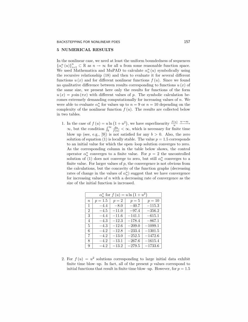
BACKSTEPPING FOR NONLINEAR PDES 157
5 NUMERICAL RESULTS
In the nonlinear case, we need at least the uniform boundedness of sequencesαni (u)ni=1 ⊂ R as n → ∞ for all u from some reasonable function space.We used Mathematica and MuPAD to calculate αnn (u) symbolically usingthe recursive relationship (18) and then to evaluate it for several differentfunctions u (x) and for different nonlinear functions f (u). Since we foundno qualitative difference between results corresponding to functions u (x) ofthe same size, we present here only the results for functions of the formu (x) = p sin (πx) with different values of p. The symbolic calculation be-comes extremely demanding computationally for increasing values of n. Wewere able to evaluate αnn for values up to n = 9 or n = 10 depending on thecomplexity of the nonlinear function f (u). The results are collected belowin two tables.
1. In the case of f (u) = u ln(1 + u2
), we have superlinearity f(u)
u
u→∞−−−−→∞, but the condition
∫∞b
duf(u) <∞, which is necessary for finite time
blow up (see, e.g., [9]) is not satisfied for any b > 0. Also, the zerosolution of equation (1) is locally stable. The value p = 1.5 correspondsto an initial value for which the open–loop solution converges to zero.As the corresponding column in the table below shows, the controloperator αnn converges to a finite value. For p = 2 the uncontrolledsolution of (1) does not converge to zero, but still αnn converges to afinite value. For larger values of p, the convergence is not obvious fromthe calculations, but the concavity of the function graphs (decreasingrates of change in the values of αnn) suggest that we have convergencefor increasing values of n with a decreasing rate of convergence as thesize of the initial function is increased.
αnn for f (u) = u ln(1 + u2
)n p = 1.5 p = 2 p = 5 p = 101 −4.4 −8.0 −40.7 −115.32 −4.5 −11.0 −97.4 −356.23 −4.4 −11.6 −141.1 −615.14 −4.3 −12.3 −178.4 −867.15 −4.3 −12.6 −209.0 −1099.16 −4.2 −12.8 −233.4 −1301.57 −4.2 −13.0 −252.5 −1472.68 −4.2 −13.1 −267.6 −1615.49 −4.2 −13.2 −279.5 −1733.6
2. For f (u) = u2 solutions corresponding to large initial data exhibitfinite time blow–up. In fact, all of the present p values correspond toinitial functions that result in finite time blow–up. However, for p = 1.5

158 PROBLEM 5.1
and p = 2, the control values seem to converge as the table belowshows. For larger values (p = 5 and p = 10), numerical calculationssuggest fast divergence.
αnn for f (u) = u2
n p = 1.5 p = 2 p = 5 p = 101 −5.6 −10.0 −62.5 −250.02 −7.2 −16.1 −221.3 −1687.03 −7.6 −18.6 −402.0 −4974.24 −8.0 −21.1 −637.3 −11202.15 −8.2 −22.6 −926.7 −22798.36 −8.3 −23.8 −1244.8 −41999.67 −8.3 −24.6 −1578.1 −70862.28 −8.4 −25.3 −1915.4 −111498.49 −8.4 −25.8 −2247.4 −165709.210 −8.5 −26.1 −2567.5 −234811.7
BIBLIOGRAPHY
[1] S. Anita and V. Barbu, “Null controllability of nonlinear convectiveheat equations,” ESAIM COCV, vol. 5, pp. 157–173, 2000.
[2] A. Balogh and M. Krstic, “Infinite dimensional backstepping–style feed-back transformations for a heat equation with an arbitrary level of in-stability,” European Journal of Control, 2002.
[3] D. Boskovic and M. Krstic, “Nonlinear stabilization of a thermal con-vection loop by state feedback,” Automatica, vol. 37, pp. 2033-2040,2001.
[4] D. Boskovic and M. Krstic, “Backstepping control of chemical tubularreactors,” Computers and Chemical Engineering, vol. 26, pp. 1077-1085,2002.
[5] D. Boskovic and M. Krstic, “Stabilization of a solid propellant rocketinstability by state feedback,” Int. J. Robust and Nonlinear Control, inpress.
[6] L.A. Caffarrelli and A. Friedman, “Blow–up of solutions of nonlinearheat equations,” J. Math. Anal. Appl., 129, pp. 409–419, 1988.
[7] M. Chipot, M. Fila, and P. Quittner, “Stationary solutions, blow up andconvergence to stationary solutions for semilinear parabolic equationswith nonlinear boundary conditions,” Acta Math. Univ. Comenianae,vol. LX, no. 1, pp. 35–103, 1991.

BACKSTEPPING FOR NONLINEAR PDES 159
[8] E. Fernandez–Cara, “Null controllability of the semilinear heat equa-tion,” ESAIM COCV, vol. 2, pp. 87–103, 1997.
[9] A. A. Lacey, “Mathematical analysis of thermal runaway for spatiallyinhomogeneous reactions,” SIAM J. Appl. Math., vol. 43, no. 6, pp.1350–1366, 1983.
[10] S. Seo, “Blowup of solutions to heat equations with nonlocal boundaryconditions,” Kobe J. Math., vol. 13, pp. 123–132, 1996.
Problem 5.2
The dynamical Lame system with boundary control:
on the structure of reachable sets
M. I. Belishev1
Dept. of the Steklov Mathematical Institute (POMI)Fontanka 27St. Petersburg [email protected]
1 MOTIVATION
The questions posed below come from dynamical inverse problems for thehyperbolic systems with boundary control. These questions arise in theframework of the BC–method, which is an approach to inverse problemsbased on their relations to the boundary control theory [1], [2].
2 GEOMETRY
Let Ω ⊂ R3 be a bounded domain with the smooth (enough) boundary Γ;λ, µ, ρ smooth functions (Lame parameters) satisfying ρ > 0, µ > 0, 3λ +2µ > 0 in Ω.The parameters determine two metrics in Ω
dl2α =|dx|2
c2α, α = p, s
where
cp :=(λ+ 2µρ
) 12
, cs :=(µ
ρ
) 12
are the velocities of p− (pressure) and s− (shear) waves; let distα be thecorresponding distances.
1Supported by the RFBR grant No. 02-01-00260.
THE DYNAMICAL LAME SYSTEM WITH BOUNDARY CONTROL 161
The distant functions (eikonals)τα(x) := distα(x,Γ), x ∈ Ω
determine the subdomainsΩTα := x ∈ Ω | τα(x) < T, T > 0
and the values Tα := infT > 0 |ΩTα = Ω, which are the times it takes forα–waves moving from Γ to fill the whole of Ω. The relation cs < cp impliesτp < τs, ΩTs ⊂ ΩTp , and Ts > Tp . If T < Ts then
∆ΩT := ΩTp \ ΩTsis a nonempty open set.If T > 0 is ’not too large’, the vector fields
να :=∇τα|∇τα|
are regular and satisfy νp(x) · νs(x) > 0, x ∈ ΩTp . Due to the latter, eachvector field (R3− valued function) u = u(x) may be represented in the form
u(x) = u(x)p + u(x)s , x ∈ ΩTp (∗)with u(x)p ‖ νp(x) and u(x)s ⊥ νs(x).
3 LAME SYSTEM. CONTROLLABILITY
Consider the dynamical system
ui tt = ρ−13∑
j,k,l=1
∂jcijkl∂luk (i = 1, 2, 3) in Ω× (0, T );
u|t=0 = ut|t=0 = 0 in Ω;u = f on Γ× [0, T ],
(∂j := ∂∂xj ) where cijkl is the elasticity tensor of the Lame model:
cijkl = λδijδkl + µ(δikδjl + δilδjk);let u = uf (x, t) = ufi (x, t)3i=1 be the solution (wave).Denote H := L2,ρ(Ω;R3) (with measure ρ dx); HT
α := y ∈ H | supp y ⊂ΩTα. As was shown in [3], the map f 7→ uf is continuous from L2(Γ ×[0, T ];R3) into C([0, T ];H). By virtue of this and due to the finiteness ofthe wave velocities, the reachable set
UT := uf (·, T ) | f ∈ L2(Γ× [0, T ];R3)is embedded into HT
p . As was proved in the same paper, the relation
clos UT ⊃ HTs
is valid for any T > 0, i.e., an approximate controllability always holds inthe subdomain ΩTs filled with the shear waves, whereas the elements of thedefect subspace
NT := HTp closH UT
(‘unreachable states’) can be supported only in ∆ΩT . On the other hand, itis not difficult to show the examples with NT 6= 0, T < Ts.

162 PROBLEM 5.2
4 PROBLEMS AND HYPOTHESES
The open problem is to characterize the defect subspace NT . The followingis the reasonable hypotheses.
• The defect space is always nontrivial: NT 6= 0 for T < Ts in thegeneral case (not only in examples). Let us note that, due to the stan-dard ‘controllability-observability’ duality, this property would meanthat in any inhomogeneous isotropic elastic media there exist the slowwaves whose forward front propagates with the velocity cs.
• In the subdomain ∆ΩT , where the elements of the defect subspaceare supported, the pressure component of the wave ( see (∗) ) deter-mines its shear component through a linear operator: uf (·, T )s =KT [uf (·, T )p] in∆ΩT . If this holds, the question is to describe theoperator KT .
• The decomposition (∗) diagonalizes the principal part of the Lamesystem.
The progress in these questions would be of great importance for the in-verse problems of the elasticity theory that is now the most difficult andchallenging class of dynamical inverse problems.
BIBLIOGRAPHY
[1] M. I. Belishev, “Boundary control in reconstruction of manifolds andmetrics (the BC-method),” Inv.Prob., 13(5):R1–R45, 1997.
[2] M. I. Belishev and A. K. Glasman, “Dynamical inverse problem for theMaxwell system: Recovering the velocity in the regular zone (the BC-method),” St.Petersburg Math. J., 12 (2):279–316, 2001.
[3] M. I. Belishev and I. Lasiecka,“The dynamical Lame system: Regularityof solutions, boundary controllability and boundary data continuation,”ESAIM COCV, 8:143–167, 2002.
Problem 5.3
Null-controllability of the heat equation in
unbounded domains
Sorin MicuFacultatea de Matematica-InformaticaUniversitatea din CraiovaAl. I. Cuza 13, Craiova, 1100Romaniasd [email protected]
Enrique ZuazuaDepartamento de Matematicas, Facultad de CienciasUniversidad AutonomaCantoblanco, 28049, [email protected]
1 DESCRIPTION OF THE PROBLEM
Let Ω be a smooth domain of Rn with n ≥ 1. Given T > 0 and Γ0 ⊂ ∂Ω,an open non-empty subset of the boundary of Ω, we consider the linear heatequation: ut −∆u = 0 in Q
u = v1Σ0 on Σu(x, 0) = u0(x) in Ω,
(1)
where Q = Ω× (0, T ), Σ = ∂Ω× (0, T ) and Σ0 = Γ0 × (0, T ) and where 1Σ0
denotes the characteristic function of the subset Σ0 of Σ.In (1) v ∈ L2(Σ) is a boundary control that acts on the system through thesubset Σ0 of the boundary and u = u(x, t) is the state.System (1) is said to be null-controllable at time T if for any u0 ∈ L2(Ω)there exists a control v ∈ L2(Σ0) such that the solution of (1) satisfies
u(x, T ) = 0 in Ω. (2)
This article is concerned with the null-controllability problem of (1) whenthe domain Ω is unbounded.
164 PROBLEM 5.3
2 MOTIVATION AND HISTORY OF THE PROBLEM
We begin with the following well-known resultTheorem 1. When Ω is a bounded domain of class C2 system (1) is null-controllable for any T > 0.We refer to D. L. Russell [12] for some particular examples treated by meansof moment problems and Fourier series and to A. Fursikov and O. Yu.Imanuvilov [3] and G. Lebeau and L. Robbiano [7] for the general resultcovering any bounded smooth domain Ω and open, nonempty subset Γ0 of∂Ω. Both the approaches of [3] and [7] are based on the use of Carlemaninequalities.However, in many relevant problems the domain Ω is unbounded. We addressthe following question: if Ω is an unbounded domain, is system (1) null-controllable for some T > 0?.None of the approaches mentioned above apply in this situation. In fact,very particular cases being excepted (see the following section), there existno results on the null-controllability of the heat equation (1) when Ω isunbounded.The approach described in [6] and [9] is also worth mentioning. In thisarticle it is proved that, for any T > 0, the heat equation has a fundamentalsolution that is C∞ away from the origin and with support in the strip0 ≤ t ≤ T . This fundamental solution, of course, grows very fast as |x|goes to infinity. As a consequence of this, a boundary controllability resultmay be immediately obtained in any domain Ω with controls distributed allalong its boundary. Note, however, that when the domain is unboundedthe solutions and controls obtained in this way grow too fast as | x |→ ∞and, therefore, these are not solutions in the classical sense. In fact, inthe frame of unbounded domains, one has to be very careful in definingthe class of admissible controlled solutions. When imposing, for instance,the classical integrability conditions at infinity, one is imposing additionalrestrictions that may determine the answer to the controllability problem.This is indeed the case, as we shall explain.There is a weaker notion of controllability property. It is the so-called ap-proximate controllability property. System (1) is said to be approximatelycontrollable in time T if for any u0 ∈ L2(Ω) the set of reachable states,R(T ;u0) = u(T ) : u solution of (1) with v ∈ L2(Σ0), is dense in L2(Ω).With the aid of classical backward uniqueness results for the heat equation(see, for instance, J.L. Lions and E. Malgrange [8] and J.M. Ghidaglia [4]),it can be seen that null-controllability implies approximate controllability.The approximate control problem for the semilinear heat equation in generalunbounded domains was addressed in [13] where an approximation methodwas developed. The domain Ω was approximated by bounded domains (es-sentially by Ω ∩ BR, BR being the ball of radius R) and the approximatecontrol in the unbounded domain Ω was obtained as limit of the approximate
NULL-CONTROLLABILITY OF THE HEAT EQUATION 165
control on the approximating bounded domain Ω ∩ BR. But this approachdoes not apply in the context of the null-control problem.However, taking into account that approximate controllability holds, it isnatural to analyze whether null-controllability holds as well.In [1] it was proved that the null-controllability property holds even in un-bounded domains if the control is supported in a subdomain that only leavesa bounded set uncontrolled. Obviously, this result is very close to the case inwhich the domain Ω is bounded and does not answer to the main issue underconsideration of whether heat processes are null-controllable in unboundeddomains.
3 AVAILABLE RESULTS
To our knowledge, in the context of unbounded domains Ω and the boundarycontrol problem, only the particular case of the half-space has been consid-ered:
Ω = Rn+ = x = (x′, xn) : x′ ∈ Rn−1, xn > 0
Γ0 = ∂Ω = Rn−1 = (x′, 0) : x′ ∈ Rn−1(3)
(see [10] for n = 1 and [11] for n > 1).According to the results in [10] and [11], the situation is completely differentto the case of bounded domains. In fact a simple argument shows that thenull controllability result which that holds for the case Ω bounded is no longertrue. Indeed, the null-controllability of (1) with initial data in L2
(Rn+)
andboundary control in L2(Σ) is equivalent to an observability inequality for theadjoint system
ϕt + ∆ϕ = 0 on Qϕ = 0 on Σ. (4)
More precisely, it is equivalent to the existence of a positive constant C > 0such that
‖ ϕ(0) ‖2L2(Rn+)≤ C
∫Σ
∣∣∣∣ ∂ϕ∂xn∣∣∣∣2 dx′dt (5)
holds for every smooth solution of (4).When Ω is bounded, Carleman inequalities provide the estimate (5) and,consequently, null-controllability holds (see, for instance, [3]). In the case ofa half-space, by using a translation argument, it is easy to see that (5) doesnot hold (see [11]).In the case of bounded domains, by using Fourier series expansion, the con-trol problem may be reduced to a moment problem. However, Fourier seriescannot be used directly in Rn+. Nevertheless, it was observed by M. Es-cobedo and O. Kavian in [2] that, on suitable similarity variables and at the

166 PROBLEM 5.3
appropriate scale, solutions of the heat equation on conical domains may beindeed developed in Fourier series on a weighted L2−space. This idea wasused in [10] and [11] to study the null-controllability property when Ω isgiven by (3).Firstly, we use similarity variables and weighted Sobolev spaces to developthe solutions in Fourier series. A sequence of one-dimensional controlledsystems like those studied in [10] is obtained. Each of these systems isequivalent to a moment problem of the following type: given S > 0 and(an)n≥1 (depending on the Fourier coefficients of the initial data u0) findf ∈ L2(0, S) such that ∫ S
0
f(s)ensds = an, ∀n ≥ 1. (6)
This moment problem turns out to be critical since it concerns the familyof real exponential functions eλnsn≥1 with λn = n, in which the usualsummability condition on the inverses of the exponents,
∑n≥1
1λn
< ∞,does not hold. It was proved that, if the sequence (an)n≥1 has the propertythat, for any δ > 0, there exists Cδ > 0 such that
|an| ≤ Cδeδn, ∀n ≥ 1, (7)
problem (6) has a solution if and only if an = 0 for all n ≥ 1.Since (an)n≥1 depend on the Fourier coeficients of the initial data, the fol-lowing negative controllability result for the one-dimensional systems is ob-tained:
Theorem 2. When Ω is the half line, there is no nontrivial initial datum u0
belonging to a negative Sobolev space that is null-controllable in finite timewith L2 boundary controls.This negative result was complemented by showing that there exist ini-tial data with exponentially growing Fourier coefficients for which null-controllability holds in finite time with L2−controls.We mention that in [10] and [11] we are dealing with solutions defined in thesense of transposition, and therefore the solutions in [6] and [9] that growand oscillate very fast at infinity are excluded.
4 OPEN PROBLEMS
As we have already mentioned, the null-controllability property of (1) whenΩ is unbounded and different from a half-line or half-space is still open.The approach based on the use of the similarity variables may still be used ingeneral conical domains. But, due to the lack of orthogonality of the tracesof the normal derivatives of the eigenfunctions, the corresponding momentproblem is more complex and remains to be solved.
NULL-CONTROLLABILITY OF THE HEAT EQUATION 167
When Ω is a general unbounded domain, the similarity transformation doesnot seem to be of any help since the domain one gets after transformationdepends on time. Therefore, a completely different approach seems to beneeded when Ω is not conical. However, one may still expect a bad behaviorof the null-control problem. Indeed, assume for instance that Ω containsRn+. If one is able to control to zero in Ω an initial data u0 by means ofa boundary control acting on ∂Ω × (0, T ), then, by restriction, one is ableto control the initial data u0 |Rn
+with the control being the restriction of
the solution in the larger domain Ω × (0, T ) to Rn−1 × (0, T ). A carefuldevelopment of this argument and of the result it may lead to remains to bedone.
ACKNOWLEDGEMENTS
The first author was partially supported by Grant PB96-0663 of DGES(Spain) and Grant A3/2002 of CNCSIS (Romania). The second author waspartially supported by Grant PB96-0663 of DGES (Spain) and the TMRnetwork of the EU “Homogenization and Multiple Scales (HMS2000).”
BIBLIOGRAPHY
[1] V. Cabanillas, S. de Menezes and E. Zuazua, “Null controllability in unboundeddomains for the semilinear heat equation with nonlinearities involving gradientterms,” J. Optim. Theory Applications, 110 (2) (2001), 245-264.
[2] M. Escobedo and O. Kavian, “Variational problems related to self-similar so-lutions of the heat equation,” Nonlinear Anal. TMA, 11 (1987), 1103-1133.
[3] A. Fursikov and O. Yu. Imanuvilov, “Controllability of evolution equations,”Lecture Notes Series #34, Research Institute of Mathematics, Global AnalysisResearch Center, Seoul National University, 1996.
[4] J. M. Ghidaglia, “Some backward uniqueness results,” Nonlinear Anal. TMA,10 (1986), 777-790.
[5] O. Yu. Imanuvilov and M. Yamamoto, “Carleman estimate for a parabolicequation in Sobolev spaces of negative order and its applications,” In: Con-trol of Nonlinear Distributed Parameter Systems, G. Chen et al. eds., Marcel-Dekker, 2000, pp. 113-137.
[6] B. F. Jones, Jr., “A fundamental solution of the heat equation which is sup-ported in a strip,” J. Math. Anal. Appl., 60 (1977), 314-324.
[7] G. Lebeau and L. Robbiano, “Controle exact de l’equation de la chaleur,”Comm. P.D.E., 20 (1995), 335-356.
[8] J. L. Lions and E. Malgrange, “Sur l’unicite retrograde dans les problemesmixtes paraboliques,” Math. Scan., 8 (1960), 277-286.
168 PROBLEM 5.3
[9] W. Littman, “Boundary control theory for hyperbolic and parabolic partial dif-ferential equations with constant coefficients,”Annali Scuola Norm. Sup. Pisa,Serie IV, 3 (1978), 567-580.
[10] S. Micu and E. Zuazua, “On the lack of null-controllability of the heat equa-tion on the half-line,” Trans. AMS, 353 (2001), 1635-1659.
[11] S. Micu and E. Zuazua, “On the lack of null-controllability of the heat equa-tion on the half-space,” Portugalia Matematica, 58 (2001), 1-24.
[12] D. L. Russell, “Controllability and stabilizability theory for linear partial dif-ferential equations. Recent progress and open questions,” em SIAM Rev., 20(1978), 639-739.
[13] L. de Teresa and E. Zuazua, “Approximate controllability of the heat equationin unbounded domains,” Nonlinear Anal. TMA, 37 (1999), 1059-1090.
Problem 5.4
Is the conservative wave equation regular?
George WeissDept. of Electrical and Electronic EngineeringImperial College LondonExhibition RoadLondon SW7 [email protected]
1 DESCRIPTION OF THE PROBLEM
We consider an infinite-dimensional system described by the wave equa-tion on an n–dimensional domain, with mixed boundary control and mixedboundary observation, which has been analyzed (as an example for a certainclass of conservative linear systems) in [13]. A somewhat simpler version ofthis system has appeared (also as an example) in the paper [11, section 7]and a related system has been discussed in [5].We assume that Ω ⊂ Rn is a bounded domain with Lipschitz boundary Γ, asdefined in Grisvard [3]. This means that, locally, after a suitable rotation ofthe orthogonal coordinate system, the boundary is the graph of a Lipschitzfunction defined on an open set in Rn−1. Such a boundary admits cornersand edges. Γ0 and Γ1 are nonempty open subsets of Γ such that Γ0∩Γ1 = ∅and Γ0 ∪ Γ1 = Γ. We denote by x the space variable (x ∈ Ω). A functionb ∈ L∞(Γ1) is given, which intuitively expresses how strongly the inputsignal acts on different parts of the active boundary Γ1. We assume thatb(x) 6= 0 for almost every x ∈ Γ1. The equations of the system are
z(x, t) = ∆z(x, t) on Ω× [0,∞),
z(x, t) = 0 on Γ0 × [0,∞),∂∂ν z(x, t) + |b(x)|2 z(x, t) =
√2 · b(x)u(x, t) on Γ1 × [0,∞),
∂∂ν z(x, t)− |b(x)|
2 z(x, t) =√
2 · b(x)y(x, t) on Γ1 × [0,∞),
z(x, 0) = z0(x), z(x, 0) = w0(x) on Ω,
(1)
where u is the input function and y is the output function. The functions
170 PROBLEM 5.4
z0 and w0 are the initial state of the system. The part Γ0 of the boundaryis just reflecting waves, while inputs and outputs act through the part Γ1.For every g ∈ H1(Ω) we denote by γg the Dirichlet trace of g on Γ (forg ∈ C1(Ω) ⊂ H1(Ω) this would simply be the restriction of g to Γ). Weregard γg as an element of L2(Γ). We define the Hilbert space
H1Γ0
(Ω) = g ∈ H1(Ω) | γg = 0 on Γ0 , ‖g‖H1 = ‖∇g‖L2 .
Proposition 1. The equations (1) determine a well-posed linear system Σwith input space U = L2(Γ1), output space Y = L2(Γ1) and state space
X = H1Γ0
(Ω)× L2(Ω) .
For the precise meaning of a well-posed linear system we refer to [8, 9, 6].These papers use the same notation and terminology that we use here, buttheir references will indicate other works in which equivalent definitions canbe found. We give a short explanation of what well-posedness means in ourcase. If we take x(0) = [z0 w0]T ∈ X, u ∈ L2([0,∞);U) and we solve theequations (1) on the time interval [0,∞), then we get x(τ) = [z(τ) z(τ)]T ∈X for every τ ≥ 0. x(τ) is called the state of the system at time τ . Moreover,if we denote the restriction of y to [0, τ ] by Pτy, then Pτy ∈ L2([0, τ ];Y ).(Note that in our particular case, U = Y .) We can introduce four familiesof bounded operators T,Φ,Ψ, and F indexed by τ ≥ 0 such that for everysuch τ ,
x(τ) = Tτx(0) + ΦτPτu, Pτy = Ψτx(0) + FτPτu.
Thus, for every τ ≥ 0, the operator matrix
Στ =[Tτ ΦτΨτ Fτ
]defines a bounded operator from X ×L2([0, τ ];U) to X ×L2([0, τ ];Y ). Thisis the essential feature of a well-posed linear system. In fact, in [8, 9, 6],Σ is defined as the family of operators Στ . For a well-posed linear system,the family T is a strongly continuous semigroup of operators acting on X.Proposition 1 was proved in [13, section 7], together with the following:
Proposition 2. The system Σ from Proposition 1 is conservative.
The fact that Σ is conservative means that the operators Στ are unitary. Inparticular, the fact that Στ is isometric means that we have
‖x(τ)‖2 − ‖x(0)‖2 =∫ τ
0
‖u(t)‖2dt−∫ τ
0
‖y(t)‖2dt ,
which can be interpreted as an energy balance equation. For background onconservative systems, we refer to [1, 2, 4, 7, 12, 13].The system Σ has, like every conservative system, a transfer function Gthat is in the Schur class. This means that G is analytic on the open right
IS THE CONSERVATIVE WAVE EQUATION REGULAR? 171
half-plane C0 and ‖G(s)‖ ≤ 1 for all s ∈ C0. For the simple proof of thisfact, see [13, theorem 1.3 and proposition 4.5]. The boundary values G(iω)can be defined for almost every ω ∈ R as nontangential limits, and we have
G(iω)∗G(iω) = G(iω)G(iω)∗ = I
for almost every ω ∈ R (i.e., G is inner and co-inner). This follows from [10,proposition 2.1] or alternatively from [7, corollary 7.3].
Recall that a well-posed linear system with input space U , output space Y ,and transfer function G is called regular if for every v ∈ U , the limit
lims→+∞, s∈R
G(s)v = Dv
exists. In this case, the operator D ∈ L(U, Y ) is called the feedthroughoperator of the system (see [8, 9, 6] for further details). For regular linearsystems, the theories of local representation, feedback and dynamic stabi-lization are much simpler than for well-posed linear systems.
Conjecture. The system Σ from Proposition 1 is regular and its feedthroughoperator is zero.
Consider the particular situation when Ω is one-dimensional: Ω = (0, 1),Γ0 = 0, Γ1 = 1 and U = Y = C. Now the function b becomes anonzero number, and without loss of generality we may take b = 1. It iseasy to see that the input signal enters the domain at x = 1, propagatesalong the domain (with unit speed) until it gets reflected at x = 0 and thenit propagates back to exit (as the output signal) at x = 1. If the initial stateis zero, then for t ≥ 2 we have y(t) = u(t−2), so that the transfer function isG(s) = e−2s. Note that G is indeed inner and it is regular with feedthroughoperator zero.The author thinks that he can prove the conjecture in the following particularcase: the active boundary Γ1 can be partitioned into a finite union of opensubsets that are either planar (i.e., an open subset of an n − 1 dimensionalhyperplane) or spherical (i.e., an open subset of an n−1 dimensional sphere).The idea is to construct solutions of (1), which locally (near a boundarypoint) look like a planar or spherical wave moving into the domain Ω (theinitial state is zero) and locally (in time and space), u is a step function.Then locally (in time and space) y is zero, which proves the claim, due tothe equivalent characterization of regularity via the step response, see [8,theorem 5.8].
BIBLIOGRAPHY
[1] D. Z. Arov and M. A. Nudelman, “Passive linear stationary dynamicalscattering systems with continous time,” Integral Equations and Oper-ator Theory, 24 (1996), pp. 1–43.
172 PROBLEM 5.4
[2] J. A. Ball, “Conservative dynamical systems and nonlinear Livsic-Brodskii nodes,” Operator Theory: Advances and Applications, 73(1994), pp. 67–95.
[3] P. Grisvard, Elliptic Problems in Nonsmooth Domains, Pitman, Boston,1985.
[4] B. M. J. Maschke and A. J. van der Schaft, “Portcontrolled Hamil-tonian representation of distributed parameter systems,” Proc. of theIFAC Workshop on Lagrangian and Hamiltonian Methods for Nonlin-ear Control, N. E. Leonard and R. Ortega, eds., Princeton UniversityPress, 2000, pp. 28–38.
[5] A. Rodriguez–Bernal and E. Zuazua, “Parabolic singular limit of a waveequation with localized boundary damping,” Discrete and ContinuousDynamical Systems, 1 (1995), pp. 303–346.
[6] O. J. Staffans and G. Weiss, “Transfer functions of regular linear sys-tems. Part II: The system operator and the Lax-Phillips semigroup,”Trans. American Math. Society, 354 (2002), pp. 3229–3262.
[7] O. J. Staffans and G. Weiss, “Transfer functions of regular linear sys-tems. Part III: Inversions and duality,” submitted.
[8] G. Weiss, “Transfer functions of regular linear systems. Part I: Charac-terizations of regularity,” Trans. American Math. Society, 342 (1994),pp. 827–854.
[9] G. Weiss, “Regular linear systems with feedback,” Mathematics of Con-trol, Signals and Systems, 7 (1994), pp. 23–57.
[10] G. Weiss, “Optimal control of systems with a unitary semigroup andwith colocated control and observation,” Systems and Control Letters,48 (2003), pp. 329–340.
[11] G. Weiss and R. Rebarber, “Optimizability and estimatability forinfinite-dimensional linear systems,” SIAM J. Control and Optimiza-tion, 39 (2001), pp. 1204–1232.
[12] G. Weiss, O. J. Staffans and M. Tucsnak, “Well-posed linear systems:A survey with emphasis on conservative systems,” Applied Mathematicsand Computer Science, 11 (2001), pp. 101–127.
[13] G. Weiss and M. Tucsnak, “How to get a conservative well-posed lin-ear system out of thin air. Part I: well-posedness and energy balance,”ESAIM COCV, vol. 9, pp. 247-74, 2003.
Problem 5.5
Exact controllability of the semi-linear wave equation
Xu ZhangDepartamento de Matematica AplicadaUniversidad Complutense28040 MadridSpainandSchool of MathematicsSichuan UniversityChengdu [email protected]
Enrique ZuazuaDepartamento de Matematicas, Facultad de CienciasUniversidad Autonoma28049 [email protected]
1 DESCRIPTION OF THE PROBLEM
Let T > 0 and Ω ⊂ Rn (n ∈ N) be a bounded domain with a C1,1 boundary∂Ω. Let ω be a proper subdomain of Ω and denote the characteristic functionof the set ω by χω. Fix a nonlinear function f ∈ C1(R).We are concerned with the exact controllability of the following semilinearwave equation: ytt −∆y + f(y) = χω(x)u(t, x) in (0, T )× Ω,
y = 0 on (0, T )× ∂Ω,y(0) = y0, yt(0) = y1 in Ω.
(1)
In (1), (y(t, ·), yt(t, ·)) is the state and u(t, ·) is the control that acts on thesystem through the subset ω of Ω.In what follows, we choose the state space and the control space as H1
0 (Ω)×L2(Ω) and L2((0, T )×Ω), respectively. Of course, the choice of these spaces is
174 PROBLEM 5.5
not unique. But this one is very natural in the context of the wave equation.The space H1
0 (Ω)× L2(Ω) is often referred to as the energy space.The exact (internal) controllability problem for (1) (in H1
0 (Ω)×L2(Ω)) maybe formulated as follows: for any given (y0, y1), (z0, z1) ∈ H1
0 (Ω) × L2(Ω),to find (if possible) a control u ∈ L2((0, T )×Ω) such that the weak solutiony of (1) satisfies
y(T ) = z0 and yt(T ) = z1 in Ω. (2)
The exact (boundary) controllability problem of (1) can be formulated simi-larly. In that case, the control u enters on the system through the boundaryconditions. This produces extra technical difficulties. The main open prob-lem on the controllability of this semilinear wave equation we shall describehere arises in both cases. We prefer to present it in the case where the controlacts on the internal subdomain ω to avoid unnecessary technical difficulties.First of all, it is well-known that when f grows too fast, the solution of (1)may blow up. In the presence of blow-up phenomena, as a consequence ofthe finite speed of propagation of solutions of (1), the exact controllability of(1) does not hold unless ω = Ω ([13]). This exception means that the controlacts on the system everywhere in Ω in which case the effect of nonlinearitymay be suppressed easily. Therefore, we suppose that
(H1) The nonlinearity f ∈ C1(R) is such that (1) admits a global weaksolution y ∈ C([0, T ];H1
0 (Ω)) ∩ C1([0, T ];L2(Ω)) for any given (y0, y1) ∈H1
0 (Ω)× L2(Ω) and u ∈ L2((0, T )× Ω).
There are two classes of conditions on f guaranteeing that (H1) holds. Thefirst one, which will be called mild growth condition, amounts to requestingthat f ∈ C1(R) grows “mildly” at infinity (see [2] and [3]), i.e.,
lim|x|→∞
∣∣∣∣∫ x
0
f(s)ds∣∣∣∣[|x|
∞∏k=1
logk(ek + x2)
]−2
<∞, (3)
where the iterated logarithm function logj is defined by the formulas
log0 s = s and logj+1 s = log(logj s), j = 0, 1, 2, · · · ,the number ej is defined by the equations logj ej = 1.It is obvious that any globally Lipschitz continuous function f satisfies (3).But, of course, (3) allows f to grow in a slight superlinear way at infinity.The second one, which will be called good sign growth condition, is the classof functions f ∈ C1(R) that grow fast at infinity but satisfy a “good-sign”condition, i.e., there exist constants L > 0, p ∈ (1, n/(n − 2)] if n ≥ 3 andp ∈ (1,∞) if n = 1, 2, such that
|f(r)− f(s)| ≤ L(1 + |r|p−1 + |s|p−1)|r − s|, ∀ r, s ∈ R (4)
and ∫ x
0
f(s)ds ≥ −Lx2 as |x| → ∞. (5)
EXACT CONTROLLABILITY OF THE SEMI-LINEAR WAVE EQUATION 175
A typical example is
f(u) = u3 for n = 1, 2, 3. (6)
On the other hand, it is well-known that, even in the linear case wheref ≡ 0, some conditions on the controllability time T and the geometry ofthe set ω where the control applies are needed in order to guarantee theexact controllability property. Thus, we assume that
(H2) T and ω are such that (1) with f ≡ 0 is exactly controllable.
There are also two classes of conditions on T and ω guaranteeing that(H2) holds. The first one, which we will call the classical multiplier con-dition, is when ω is a neighborhood of a subset of the boundary of the formΓ(x0) = x ∈ ∂Ω : (x− x0) · ν(x) > 0 for some x0 ∈ Rn, where ν(x) is theunit outward normal vector to ∂Ω at x, and T > 2 max|x−x0| : x ∈ Ω \ ω.This is the typical situation one encounters when applying the multipliertechnique ([8]). The second one is when T and Ω satisfy the so-called Geo-metric Control Condition introduced in [1].We have the following
Open Problem: Do (H1) and (H2) imply the exact controllability of (1)?
The above problem can also be formulated in the more general case in whichthe nonlinearity is of the form f(t, x, y, yt,∇y). Of course, the problemis even more difficult in that case and new phenomena may occur due tothe strong dissipative effects that terms of the form |ut|p−1ut may produce.Thus, we shall focus in the case f = f(y). This open problem will be mademore precise below.
2 AVAILABLE RESULTS AND OPEN PROBLEMS
Nonlinearities with mild growth condition
For the one space dimensional case, by combining the sidewise energy esti-mates for the 1 − d wave equations and the fixed point technique, Zuazua([13]) obtained the following result:
Theorem 1: Assume n = 1 and Ω = (0, 1). Let (a, b) be a (proper) subin-terval of (0, 1), T > 2 max(a, 1− b) and
lim|x|→∞
|f(x)||x|−1 log−2 |x| = 0. (7)
Then (1) is exact controllable.
Later on, based on a method due to Emanuilov ([5]), Cannarsa, Komornik,and Loreti ([2]) improved theorem 1 by relaxing the growth condition on f .The main result in [2] says that the same conclusion in theorem 1 holds ifthe condition (7) on f is replaced by (3). The growth condition (3) on f is
176 PROBLEM 5.5
sharp (since solutions of (1) may blow up whenever f grows faster than (3)at infinity and f has the bad sign).For the higher dimensional case, Li and Zhang ([7]) proved the followingresult:
Theorem 2: Let ω be a neighborhood of ∂Ω, T > diam(Ω \ ω) andlim
|x|→∞f(x)|x|−1 log−1/2 |x| = 0. (8)
Then (1) is exactly controllable.
A special case of theorem 2 is when f is globally Lipschitz continuous, whichgives the main result of Zuazua in [12]. The main result in [12] was gener-alized to an abstract setting by Lasiecka and Triggiani ([6]) using a globalversion of Inverse Function theorem and was extended in [9] to the case whenT and ω satisfy the classical multiplier condition.It is natural to conjecture that the same conclusion in Theorem 2 holds underthe growth condition (3) on f as in one dimension. But this is by now an openproblem. On the other hand, whether the same conclusion in theorem 2 holdsfor more general conditions on T and ω, say the classical multiplier conditionor Geometric Control Condition, is also an open problem. Especially, whenT and ω satisfy the Geometric Control Condition, the exact controllabilityproblem for (1) is open even for globally Lipschitz continuous nonlinearities.
Nonlinearities with good sign and superlinear growth at infinity
In this case, there are no global exact controllability results in the literature.However, using a fixed point argument, Zuazua proved the following localexact controllability results for (1) ([10]):
Theorem 3: Let (H2) hold, f ∈ C1(R) satisfy (4) and f(0) = 0. Thenthere is a δ > 0 such that for any (y0, y1) and (z0, z1) in H1
0 (Ω) × L2(Ω)with |(y0, y1)|H1
0 (Ω)×L2(Ω) + |(z0, z1)|H10 (Ω)×L2(Ω) ≤ δ, there is a control u ∈
L2((0, T )× Ω), such that (2) holds.
Combining theorem 3 and the stabilization results for the semilinear waveequations with “good-sign” condition on the nonlinearity ([11] and [4]), it iseasy to show that
Theorem 4: Let T0 and ω satisfy the classical multiplier condition and fsatisfy (4)–(5). Then for any (y0, y1) and (z0, z1) in H1
0 (Ω) × L2(Ω), thereexist a time T ≥ T0 and a control u(·) ∈ L2((0, T )×Ω), such that (2) holds.
Note that the controllability time T in theorem 4 depends on (y0, y1) and(z0, z1). According to [11], one can obtain explicit bounds on T . However,whether T may be chosen to be uniform, i.e., independent of the data (y0, y1)and (z0, z1), is an open problem even for the nonlinearity in (6) for n = 1.This is certainly one of the main open problems in the context of controlla-bility of nonlinear PDE.
EXACT CONTROLLABILITY OF THE SEMI-LINEAR WAVE EQUATION 177
ACKNOWLEDGEMENTS
This work was supported in part by the grants PB96-0663 of the DGES(Spain), the EU TMR Project “Homogenization and Multiple Scales,” aFoundation for the Authors of Excellent Ph.D. Theses in China, and theNSF of China (19901024).
BIBLIOGRAPHY
[1] C. Bardos, G. Lebeau, and J. Rauch, “Sharp sufficient conditions forthe observation, control, and stabilization of waves from the boundary,”SIAM J. Control Optim., 30, pp. 1024-1065, 1992.
[2] P. Cannarsa, V. Komornik, and P. Loreti, “One-sided and internal con-trollability of semilinear wave equations with infinitely iterated loga-rithms,” Preprint.
[3] T. Cazenave and A. Haraux, “Equations d’evolution avec non linearitelogarithmique,” Ann. Fac. Sci. Toulouse, 2, pp. 21-51, 1980.
[4] B. Dehman, G. Lebeau, and E. Zuazua, “Stabilization and control forthe subcritical semilinear wave equation,” Preprint, 2002.
[5] O. Yu. Emanuilov, “Boundary controllability of semilinear evolutionequations,” Russian Math. Surveys, 44, pp. 183-184, 1989.
[6] I. Lasiecka and R. Triggiani, “Exact controllability of semilinear abstractsystems with application to waves and plates boundary control prob-lems,” Appl. Math. Optim., 23, pp. 109-154, 1991.
[7] L. Li and X. Zhang, “Exact controllability for semilinear wave equa-tions,” J. Math. Anal. Appl., 250, pp. 589-597, 2000.
[8] J. L. Lions, Controlabilite exacte, perturbations et systemes distribues,Tome 1, Rech. Math. Appl. 8, Masson, Paris, 1988.
[9] X. Zhang, “Explicit observability estimate for the wave equation withpotential and its application,” R. Soc. Lond. Proc. Ser. A Math. Phys.Eng. Sci., 456, pp. 1101-1115, 2000.
[10] E. Zuazua, “Exact controllability for the semilinear wave equation,” J.Math. Pures Appl., 69, pp. 1-31, 1990.
[11] E. Zuazua, “Exponential decay for semilinear wave equations with local-ized damping,” Comm. Partial Differential Equations, 15, pp. 205-235,1990.
[12] E. Zuazua, “Exact boundary controllability for the semilinear waveequation,” In: Nonlinear partial differential equations and their applica-
178 PROBLEM 5.5
tions, College de France Seminar, vol. X (Paris, 1987-1988), pp. 357-391,Pitman Res. Notes Math. Ser., 220, Longman Sci. Tech., Harlow, 1991.
[13] E. Zuazua, “Exact controllability for semilinear wave equations in onespace dimension,” Ann. Inst. H. Poincare Anal. Non Lineaire, 10, pp.109-129, 1993.
Problem 5.6
Some control problems in electromagnetics and fluid
dynamics
Lorella FatoneDipartimento di Matematica Pura ed ApplicataUniversita di Modena e Reggio EmiliaVia Campi 213/b, 41100 Modena (MO)[email protected]
Maria Cristina RecchioniIstituto di Teoria delle Decisioni e Finanza Innovativa (DE.F.IN.)Universita di AnconaPiazza Martelli 8, 60121 Ancona (AN)[email protected]
Francesco ZirilliDipartimento di Matematica “G. Castelnuovo”Universita di Roma “La Sapienza”Piazzale Aldo Moro 2, 00185 [email protected]
1 INTRODUCTION
In recent years, as a consequence of the dramatic increases in computingpower and of the continuing refinement of the numerical algorithms avail-able, the numerical treatment of control problems for systems governed bypartial differential equation; see, for example, [1], [3], [4], [5], [8]. The impor-tance of these mathematical problems in many applications in science andtechnology cannot be overemphasized.The most common approach to a control problem for a system governedby partial differential equations is to see the problem as a constrained non-linear optimization problem in infinite dimension. After discretization the

180 PROBLEM 5.6
problem becomes a finite dimensional constrained nonlinear optimizationproblem that can be attacked with the usual iterative methods of nonlin-ear optimization, such as Newton or quasi-Newton methods. Note that theproblem of the convergence, when the “discretization step goes to zero,” ofthe solutions computed in finite dimension to the solution of the infinitedimensional problem is a separate question and must be solved separately.When this approach is used an objective function evaluation in the nonlin-ear optimization procedure involves the solution of the partial differentialequations that govern the system. Moreover, the evaluation of the gradientor Hessian of the objective function involves the solution of some kind ofsensitivity equations for the partial differential equations considered. Thenonlinear optimization procedure that usually involves function, gradientand Hessian evaluation is computationally very expensive.This fact is a serious limitation to the use of control problems for systemsgoverned by partial differential equations in real situations. However the ap-proach previously described is very straightforward and does not use any ofthe special features present in every system governed by partial differentialequations. So that, at least in some special cases, it should be possible toimprove on this straightforward approach.The purpose of this paper is to point out a problem, see [6], [2], where anew approach, that greatly improves on the previously described one, hasbeen introduced and to suggest some other problems where, hopefully, sim-ilar improvements can be obtained. In particular, we propose two controlproblems of great relevance in several applications in science and technologyand we suggest the (open) question of characterizing the optimal solution ofthese control problems as the solution of suitable systems of partial differen-tial equations. If this question has an affirmative answer, high performancealgorithms can be developed to solve the control problems proposed. Notethat in [6], [2] this characterization has been made for some control problemsin acoustics, thanks to the use of the Pontryagin maximum principle, andhas permitted to develop high performance algorithms to solve these con-trol problems. Moreover, we suggest the (open) question of using effectivelythe dynamic programming method to derive closed loop control laws for thecontrol problems considered. For effective use of the dynamic programmingmethod, we mean the possibility of computing a closed loop control law atapproximately the same computational cost of solving the original problemwhen no control strategy is involved.In section 2 we summarize the results obtained in [6], [2], and in section 3we present two problems that we believe can be approached in a way similarto the one described in [6], [2].
SOME CONTROL PROBLEMS IN ... 181
2 PREVIOUS RESULTS
In [6], [2] a furtivity problem in time dependent acoustic obstacle scatter-ing is considered. An obstacle of known acoustic impedance is hit by aknown incident acoustic field. When hit by the incident acoustic field, theobstacle generates a scattered acoustic field. To make the obstacle furtivemeans to “minimize” the scattered field. The furtivity effect is obtainedcirculating on the boundary of the obstacle a “pressure current” that is aquantity whose physical dimension is: pressure divided by time. The prob-lem consists in finding the optimal “pressure current” that “minimizes” thescattered field and the “size” of the pressure current employed. The mathe-matical model used to study this problem is a control problem for the waveequation, where the control function (i.e., the pressure current) influencesthe state variable (i.e., the scattered field) through a boundary conditionimposed on the boundary of the obstacle, and the cost functional dependsexplicitly from both the state variable and the control function. Introducingan auxiliary variable and using the Pontryagin maximum principle (see [7])in [6], [2] it is shown that the optimal control of this problem can be obtainedfrom the solution of a system of two coupled wave equations. This systemof wave equations is equipped with suitable initial, final, and boundary con-ditions. Thanks to this ingenious construction the solution of the optimalcontrol problem can be obtained solving the system of wave equations with-out the necessity of going through the iterations implied in general by thenonlinear optimization procedure. This fact avoids many of the difficulties,that have been mentioned above, present in the general case. Finally, thesystem of wave equations is solved numerically using a highly parallelizablealgorithm based on the operator expansion method (for more details, see[6], [2] and the references therein). Some numerical results obtained withthis algorithm on simple test problems can be seen in the form of com-puter animations in the websites: http://www.econ.unian.it/recchioni/w6,http://www.econ.unian.it/recchioni/w8. In the following section, we suggesttwo problems where will be interesting to carry out a similar analysis.
3 TWO CONTROL PROBLEMS
Let R be the set of real numbers, x = (x1, x2, x3)T ∈ R3 (where the su-perscript T means transposed) be a generic vector of the three-dimensionalreal Euclidean space R3, and let (·, ·), ‖ · ‖ and [·, ·] denote the Euclideanscalar product, the Euclidean vector norm and the vector product in R3,respectively.The first problem suggested is a “masking” problem in time-dependent elec-tromagnetic scattering. Let Ω ⊂ R3 be a bounded simply connected openset (i.e., the obstacle) with locally Lipschitz boundary ∂Ω. Let Ω denotethe closure of Ω and n(x) = (n1(x), n2(x), n3(x))T ∈ R3, x ∈ ∂Ω be the
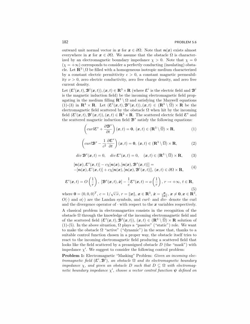
182 PROBLEM 5.6
outward unit normal vector in x for x ∈ ∂Ω. Note that n(x) exists almosteverywhere in x for x ∈ ∂Ω. We assume that the obstacle Ω is character-ized by an electromagnetic boundary impedance χ > 0. Note that χ = 0(χ = +∞) corresponds to consider a perfectly conducting (insulating) obsta-cle. Let R3 \Ω be filled with a homogeneous isotropic medium characterizedby a constant electric permittivity ε > 0, a constant magnetic permeabil-ity ν > 0, zero electric conductivity, zero free charge density, and zero freecurrent density.Let (Ei(x, t),Bi(x, t)), (x, t) ∈ R3×R (where Ei is the electric field and Bi
is the magnetic induction field) be the incoming electromagnetic field prop-agating in the medium filling R3 \ Ω and satisfying the Maxwell equations(1)-(3) in R3 × R. Let (Es(x, t),Bs(x, t)), (x, t) ∈ (R3 \ Ω) × R be theelectromagnetic field scattered by the obstacle Ω when hit by the incomingfield (Ei(x, t),Bi(x, t)), (x, t) ∈ R3 ×R. The scattered electric field Es andthe scattered magnetic induction field Bs satisfy the following equations:(
curlEs +∂Bs
∂t
)(x, t) = 0, (x, t) ∈ (R3 \ Ω)×R, (1)
(curlBs − 1
c2∂Es
∂t
)(x, t) = 0, (x, t) ∈ (R3 \ Ω)×R, (2)
divBs(x, t) = 0, divEs(x, t) = 0, (x, t) ∈ (R3 \ Ω)×R, (3)
[n(x),Es(x, t)]− cχ[n(x), [n(x),Bs(x, t)]] =−[n(x),Ei(x, t)] + cχ[n(x), [n(x),Bi(x, t)]], (x, t) ∈ ∂Ω×R,
(4)
Es(x, t) = O
(1r
), [Bs(x, t), x]− 1
cEs(x, t) = o
(1r
), r → +∞, t ∈ R,
(5)where 0 = (0, 0, 0)T , c = 1/
√ε ν, r = ‖x‖, x ∈ R3, x = x
‖x‖ , x 6= 0,x ∈ R3,O(·) and o(·) are the Landau symbols, and curl· and div· denote the curland the divergence operator of · with respect to the x variables respectively.A classical problem in electromagnetics consists in the recognition of theobstacle Ω through the knowledge of the incoming electromagnetic field andof the scattered field (Es(x, t),Bs(x, t)), (x, t) ∈ (R3 \ Ω) × R solution of(1)-(5). In the above situation, Ω plays a “passive” (“static”) role. We wantto make the obstacle Ω “active” (“dynamic”) in the sense that, thanks to asuitable control function chosen in a proper way, the obstacle itself tries toreact to the incoming electromagnetic field producing a scattered field thatlooks like the field scattered by a preassigned obstacle D (the “mask”) withimpedance χ′. We suggest to consider the following control problem:Problem 1: Electromagnetic “Masking” Problem: Given an incoming elec-tromagnetic field (Ei,Bi), an obstacle Ω and its electromagnetic boundaryimpedance χ, and given an obstacle D such that D ⊆ Ω with electromag-netic boundary impedance χ′, choose a vector control function ψ defined on

SOME CONTROL PROBLEMS IN ... 183
the boundary of the obstacle ∂Ω for t ∈ R and appearing in the boundarycondition satisfied by the scattered electromagnetic field on ∂Ω, in order tominimize a cost functional that measures the “difference” between the elec-tromagnetic field scattered by Ω, i.e., (Es,Bs), and the electromagnetic fieldscattered by D, i.e., (EsD,B
sD), when Ω and D respectively are hit by the in-
coming field (Ei,Bi), and the “size” of the vector control function employed.The control function ψ has the physical dimension of an electric field and theaction of the optimal control electric field on the boundary of the obstaclemakes the obstacle “active” (“dynamic”) and able to react to the incidentelectromagnetic field to become “unrecognizable,” that is “Ω will do its bestto appear as his mask D.”The second control problem we suggest to consider is a control problem influid dynamics. Let us consider an obstacle Ωt, t ∈ R, that is a rigid body, as-sumed homogeneous, moving in R3 with velocity υ = υ(x, t), (x, t) ∈ Ωt×R.Moreover for t ∈ R the obstacle Ωt ⊂ R3 is a bounded simply connectedopen set. For t ∈ R let ξ = ξ(t) be the position of the center of massof the obstacle Ωt. The motion of the obstacle is completely described bythe velocity w = w(ξ, t), t ∈ R of the center of mass of the obstacle (i.e.,
w =dξ
dt, t ∈ R), the angular velocity ω = ω(ξ, t), t ∈ R of the obstacle
around the instantaneous rotation axis going through the center of massξ = ξ(t), t ∈ R and the necessary initial conditions. Note that the velocitiesof the points belonging to the obstacle υ(x, t), (x, t) ∈ Ωt ×R can be ex-pressed in terms of w(ξ, t),ω(ξ, t), t ∈ R. Let R3 \Ωt, t ∈ R be filled with aNewtonian incompressible viscous fluid of viscosity η. We assume that boththe density of the fluid and the temperature are constant. For example,Ωt, t ∈ R can be a submarine or an airfoil immersed in an incompressibleviscous fluid. Let v = (v1, v2, v3)T and p be the velocity field and the pres-sure field of the fluid, respectively, f be the density of the external forcesper mass unit acting on the fluid, and v−∞ be an assigned solenoidal vectorfield. We assume that in the limit t → −∞ the body Ωt is at rest in theposition Ω−∞. Under these assumptions, we have that in the reference framegiven by x = (x1, x2, x3)T the following system of Navier-Stokes equationsholds:
∂v
∂t(x, t) + (v(x, t),∇)v(x, t)− η∆v(x, t) +∇p(x, t) = f(x, t),
(x, t) ∈ (R3 \ Ωt)×R ,(6)
div v(x, t) = 0, (x, t) ∈ (R3 \ Ωt)×R , (7)
limt→−∞
v(x, t) = v−∞(x), x ∈ R3 \Ω−∞ ,v(x, t) = υ(x, t), (x, t) ∈ ∂Ωt×R.
(8)
In (6) we have ∇ =(
∂∂x1
, ∂∂x2
, ∂∂x3
)Tand
(v,∇)v =
3∑j=1
vj∂v1∂xj
,3∑j=1
vj∂v2∂xj
,3∑j=1
vj∂v3∂xj
T
.
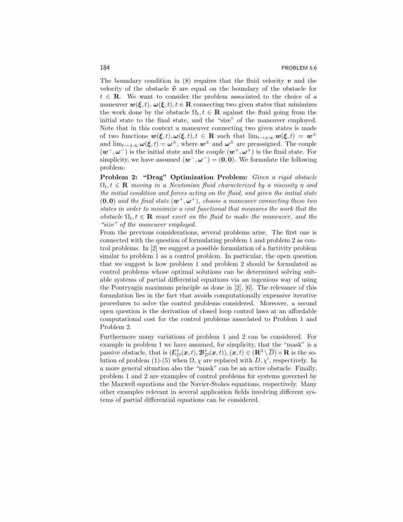
184 PROBLEM 5.6
The boundary condition in (8) requires that the fluid velocity v and thevelocity of the obstacle υ are equal on the boundary of the obstacle fort ∈ R. We want to consider the problem associated to the choice of amaneuver w(ξ, t), ω(ξ, t), t ∈ R connecting two given states that minimizesthe work done by the obstacle Ωt, t ∈ R against the fluid going from theinitial state to the final state, and the “size” of the maneuver employed.Note that in this context a maneuver connecting two given states is madeof two functions w(ξ, t),ω(ξ, t), t ∈ R such that limt→±∞w(ξ, t) = w±
and limt→±∞ ω(ξ, t) = ω±, where w± and ω± are preassigned. The couple(w−,ω−) is the initial state and the couple (w+,ω+) is the final state. Forsimplicity, we have assumed (w−,ω−) = (0,0). We formulate the followingproblem:Problem 2: “Drag” Optimization Problem: Given a rigid obstacleΩt, t ∈ R moving in a Newtonian fluid characterized by a viscosity η andthe initial condition and forces acting on the fluid, and given the initial state(0,0) and the final state (w+,ω+), choose a maneuver connecting these twostates in order to minimize a cost functional that measures the work that theobstacle Ωt, t ∈ R must exert on the fluid to make the maneuver, and the“size” of the maneuver employed.From the previous considerations, several problems arise. The first one isconnected with the question of formulating problem 1 and problem 2 as con-trol problems. In [2] we suggest a possible formulation of a furtivity problemsimilar to problem 1 as a control problem. In particular, the open questionthat we suggest is how problem 1 and problem 2 should be formulated ascontrol problems whose optimal solutions can be determined solving suit-able systems of partial differential equations via an ingenious way of usingthe Pontryagin maximum principle as done in [2], [6]. The relevance of thisformulation lies in the fact that avoids computationally expensive iterativeprocedures to solve the control problems considered. Moreover, a secondopen question is the derivation of closed loop control laws at an affordablecomputational cost for the control problems associated to Problem 1 andProblem 2.Furthermore many variations of problem 1 and 2 can be considered. Forexample in problem 1 we have assumed, for simplicity, that the “mask” is apassive obstacle, that is (EsD(x, t),Bs
D(x, t)), (x, t) ∈ (R3 \D)×R is the so-lution of problem (1)-(5) when Ω, χ are replaced with D,χ′, respectively. Ina more general situation also the “mask” can be an active obstacle. Finally,problem 1 and 2 are examples of control problems for systems governed bythe Maxwell equations and the Navier-Stokes equations, respectively. Manyother examples relevant in several application fields involving different sys-tems of partial differential equations can be considered.
SOME CONTROL PROBLEMS IN ... 185
BIBLIOGRAPHY
[1] T. S. Angell, A. Kirsch, and R. E. Kleinman, “Antenna control andoptimization,” Proceedings of the IEEE, 79, pp. 1559-1568,1991.
[2] L. Fatone, M. C. Recchioni, and F. Zirilli, “Furtivity and masking prob-lems in time dependent acoustic obstacle scattering,” forthcoming inThird ISAAC Congress Proceedings.
[3] J. W. He, R. Glowinski, R. Metcalfe, A. Nordlander, and J. Periaux,“Active control and drag optimization for flow past a circular cylinder,”Journal of Computational Physics, 163, pp. 83-117, 2000.
[4] J. E. Lagnese, “A singular perturbation problem in exact controllabilityof the Maxwell system,” ESAIM Control, Optimization and Calculus ofVariations, 6, pp. 275-289, 2001.
[5] J. Luniley and P. Blossery, “Control of turbulence,” Annual Review ofFluid Mechanics, 30, pp. 311-327, 1998.
[6] F. Mariani, M. C. Recchioni, and F. Zirilli, “The use of the Pontryaginmaximum principle in a furtivity problem in time-dependent acousticobstacle scattering,” Waves in Random Media, 11, pp. 549-575, 2001.
[7] L. Pontriaguine, V. Boltianski, R. Gamkrelidze, and F. Micktckenko,Theorie Mathematique des Processus Optimaux, Editions Mir, Moscow,1974.
[8] S. S. Sritharan, “An introduction to deterministic and stochastic controlof viscous flow,” In: Optimal Control of Viscous Flow, S. S. Sritharaneds., SIAM, Philadelphia, pp. 1-42, 1998.


PART 6
Stability, Stabilization

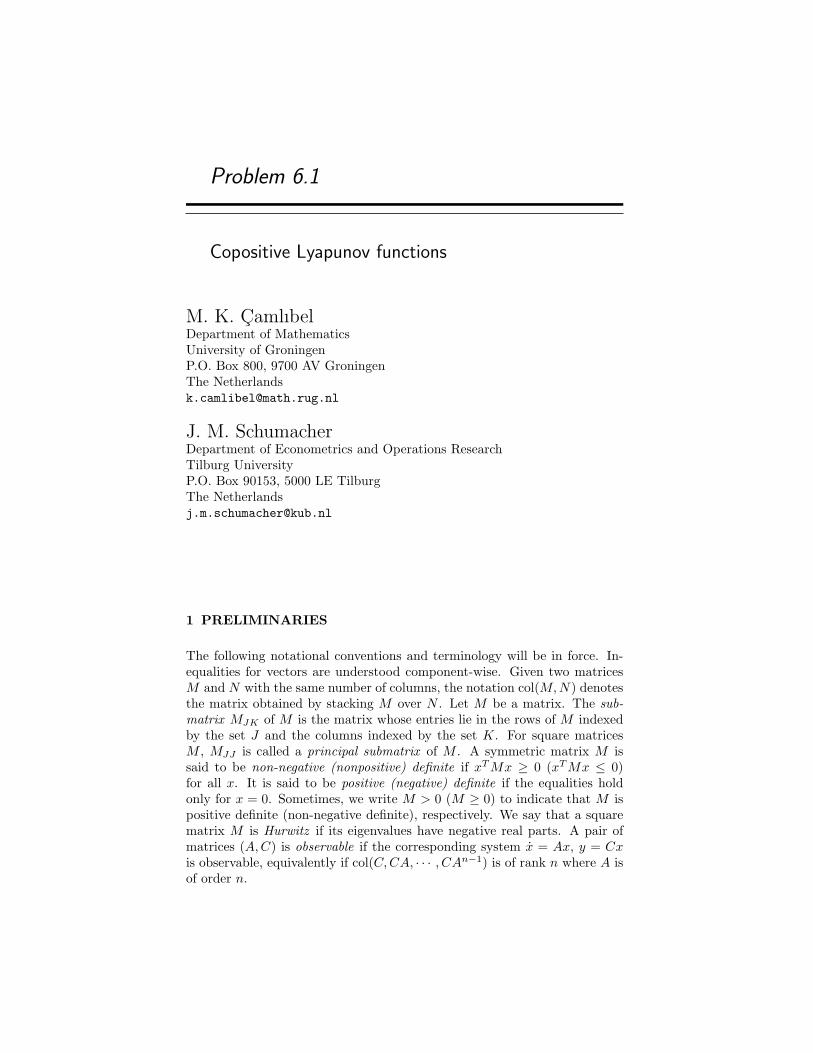
Problem 6.1
Copositive Lyapunov functions
M. K. CamlıbelDepartment of MathematicsUniversity of GroningenP.O. Box 800, 9700 AV GroningenThe [email protected]
J. M. SchumacherDepartment of Econometrics and Operations ResearchTilburg UniversityP.O. Box 90153, 5000 LE TilburgThe [email protected]
1 PRELIMINARIES
The following notational conventions and terminology will be in force. In-equalities for vectors are understood component-wise. Given two matricesM and N with the same number of columns, the notation col(M,N) denotesthe matrix obtained by stacking M over N . Let M be a matrix. The sub-matrix MJK of M is the matrix whose entries lie in the rows of M indexedby the set J and the columns indexed by the set K. For square matricesM , MJJ is called a principal submatrix of M . A symmetric matrix M issaid to be non-negative (nonpositive) definite if xTMx ≥ 0 (xTMx ≤ 0)for all x. It is said to be positive (negative) definite if the equalities holdonly for x = 0. Sometimes, we write M > 0 (M ≥ 0) to indicate that M ispositive definite (non-negative definite), respectively. We say that a squarematrix M is Hurwitz if its eigenvalues have negative real parts. A pair ofmatrices (A,C) is observable if the corresponding system x = Ax, y = Cxis observable, equivalently if col(C,CA, · · · , CAn−1) is of rank n where A isof order n.
190 PROBLEM 6.1
2 MOTIVATION
Lyapunov stability theory is one of the ever green topics in systems andcontrol. For (finite dimensional) linear systems, the following theorem isvery well-known.Theorem 1:[3, Theorem 1.2]: The following conditions are equivalent.
1. The system x = Ax is asymptotically stable.
2. The Lyapunov equation ATP + PA = Q has a positive definite sym-metric solution P for any negative definite symmetric matrix Q.
As a refinement, we can replace the last statement by
2′. The Lyapunov equation ATP+PA = Q has a positive definite symmet-ric solution P for any nonpositive definite symmetric matrix Q suchthat the pair (A,Q) is observable.
An interesting application is to the stability of the so-called switched systems.Consider the system
x = Aσx (1)
where the switching signal σ : [0,∞) → 1, 2 is a piecewise constant func-tion. We assume that it has a finite number of discontinuities over finitetime intervals in order to rule out infinitely fast switching. A strong notionof stability for the system (1) is the requirement of stability for arbitraryswitching signals.The dynamics of (1) coincides with one of the linear subsystems if the switch-ing signal is constant, i.e., there are no switchings at all. This leads usto an obvious necessary condition: stability of each subsystem. Anotherextreme case would emerge if there exists a common Lyapunov functionfor the subsystems. Indeed, such a Lyapunov function would immediatelyprove the stability of (1). An earlier paper [8] pointed out the importance ofcommutation relations between A1 and A2 in finding a common Lyapunovfunction. More precisely, it has been shown that if A1 and A2 are Hur-witz and commutative then they admit a common Lyapunov function. In[1, 6], the commutation relations of subsystems are studied further in a Liealgebraic framework and sufficient conditions for the existence of a commonLyapunov function are presented. Notice that the results of [1] are strongerthan those in [6]. However, we prefer to restate [6, Theorem 2] for simplicity.
Theorem 2: If Ai is a Hurwitz matrix for i = 1, 2 and the Lie algebraA1, A2LA is solvable then there exists a positive definite matrix P suchthat ATi P + PAi < 0 for i = 1, 2.

COPOSITIVE LYAPUNOV FUNCTIONS 191
So far, we quoted some known results. Our main goal is to pose two openproblems that can be viewed as extensions of Theorems 2 and 2 for a classof piecewise linear systems. More precisely, we will consider systems of theform
x = Aix for Cix ≥ 0 i = 1, 2. (2)
Here the cones Ci = x | Cix ≥ 0 do not necessarily cover the wholex-space. We assume that
a. there exists a (possibly discontinuous) function f such that (2) can bedescribed by x = f(x) for all x ∈ C1 ∪ C2, and
b. for each initial state x0 ∈ C1 ∪ C2, there exists a unique solution x inthe sense of Caratheodory, i.e., x(t) = x0 +
∫ t0f(x(τ)) dτ .
A natural example[b.] of such piecewise linear dynamics is a linear comple-mentarity system (see [9]) of the form
x = Ax+Bu, y = Cx+Du
(u(t) ≥ 0) and (y(t) ≥ 0) and (u(t) = 0 or y(t) = 0) for all t ≥ 0
where A ∈ Rn×n, B ∈ Rn×1, C ∈ R1×n, and D ∈ R. If D > 0 this systemcan be put into the form of (2) with A1 = A, C1 = C, A2 = A − BD−1C,and C2 = −C. Equivalently, it can be described by
x = f(x) (3)
where f(x) = Ax if Cx ≥ 0 and f(x) = (A − BD−1C)x if Cx ≤ 0. Notethat f is Lipschitz continuous and hence (3) admits a unique (continuouslydifferentiable) solution x for all initial states x0.One way of studying the stability of the system (2) is simply to utilizeTheorem 2. However, there are some obvious drawbacks:
i. It requires positive definiteness of the common Lyapunov functionwhereas the positivity on a cone is enough for the system (2).
ii. It considers any switching signal whereas the initial state determinesthe switching signal in (2).
In the next section, we focus on ways of eliminating the conservatism men-tioned in 2.
3 DESCRIPTION OF THE PROBLEMS
First, we need to introduce some nomenclature. A matrix M is said tobe copositive (strictly copositive) with respect to a cone C if xTMx ≥ 0
(xTMx > 0) for all nonzero x ∈ C. We use the notation MC< 0 and M
C 0
192 PROBLEM 6.1
respectively for copositivity and strict copositivity. When the cone C is clearfrom the context we just write < or .The first problem that we propose calls for an extension of Theorem 2 forlinear dynamics restricted to a cone.
Problem 1: Let a square matrix A and a cone C = x | Cx ≥ 0 begiven. Determine necessary and sufficient conditions for the existence of asymmetric matrix P such that P 0 and ATP + PA ≺ 0.An immediate necessary condition for the existence of such a matrix P is thatthe matrix A should not have any eigenvectors in the cone C correspondingto its positive eigenvalues.Once Problem 3 solved, it would be natural to take a step further by at-tempting to extend Theorem 2 to the systems (2). In other words, it wouldbe natural to attack the following problem.
Problem 2: Let two square matrices A1, A2, and two cones C1 = x |C1x ≥ 0, C2 = x | C2x ≥ 0 be given. Determine sufficient conditions for
the existence of a symmetric matrix P such that PCi 0 and ATi P +PAi
Ci≺ 0for i = 1, 2.
4 ON COPOSITIVE MATRICES
This last section discusses copositive matrices in order to provide a startingpoint for further investigation of the proposed problems.The class of copositive matrices occurs in optimization theory and particu-larly in the study of the linear complementarity problem [2]. We quote from[4] the following theorem which provides a characterization of copositivematrices.Theorem 2. A symmetric matrix M is (strictly) copositive with respect tothe cone x | x ≥ 0 if and only if every principal submatrix of M has noeigenvector v > 0 with associated eigenvalue (λ ≤ 0) λ < 0.Since the number of principal submatrices of a matrix of order n is roughly2n, this result has a practical disadvantage. In fact, Murty and Kabadi [7]showed that testing for copositivity is NP-complete. An interesting subclassof copositive matrices are the ones that are equal to the sum of a nonnegativedefinite matrix and a non-negative matrix. This class of matrices is studiedin [5] where a relatively more tractable algorithm has been presented forchecking if a given matrix belongs to the class or not.
COPOSITIVE LYAPUNOV FUNCTIONS 193
BIBLIOGRAPHY
[1] A. A. Agrachev and D. Liberzon, “Lie-algebraic stability criteria forswitched systems,” SIAM J. Control Optim., 40(1):253–269, 2001.
[2] R. W. Cottle, J.-S. Pang, and R. E. Stone, The Linear ComplementarityProblem, Academic Press, Inc., Boston, 1992.
[3] Z. Gajic and M. T. J. Qureshi, Lyapunov Matrix Equation in SystemStability and Control, volume 195 of Mathematics in Science and Engi-neering, Academic Press, San Diego, 1995.
[4] W. Kaplan, “A test for copositive matrices,” Linear Algebra Appl.,313:203–206, 2000.
[5] W. Kaplan, “A copositivity probe,” Linear Algebra Appl., 337:237–251,2001.
[6] D. Liberzon, J. P. Hespanha, and A. S. Morse, “Stability of switchedsystems: A Lie-algebraic condition,” Systems Control Lett., 37:117–122,1999.
[7] K. Murty and S. N. Kabadi, “Some NP-complete problems in quadraticand nonlinear programming,” Math. Programming, 39:117–129, 1987.
[8] K. S. Narendra and J. Balakrishnan, “A common Lyapunov functionfor stable LTI systems with commuting A-matrices,” IEEE Trans. Au-tomatic Control, 39:2469–2471, 1994.
[9] A. J. van der Schaft and J. M. Schumacher, “Complementarity mod-elling of hybrid systems,” IEEE Transactions on Automatic Control,43(4):483–490, 1998.
Problem 6.2
The strong stabilization problem for linear
time-varying systems
Avraham FeintuchDepartment of MathematicsBen-Gurion University of the [email protected]
1 DESCRIPTION OF THE PROBLEM
I will formulate the strong stabilization problem in the formalism of theoperator theory of systems. In this framework, a linear system is a lineartransformation L acting on a Hilbert spaceH that is equipped with a naturaltime structure, which satisfies the standard physical realizability conditionknown as causality. To simplify the formulation, we choose H to be thesequence space l2[0,∞) = < x0, x1, · · · > : xi ∈ Cn,
∑‖xi‖2 <∞ and de-
note by Pn the truncation projection onto the subspace generated by the firstn vectors e0, · · · , en of the standard orthonormal basis on H. Causalityof L is expressed as PnL = PnLPn for all non-negative integers n. A linearsystem L is stable if it is a bounded operator on H. A fundamental issue thatwas studied in both classical and modern control theory was that of internalstabilization of unstable systems by feedback. It is generally acknowledgedthat the paper of Youla et al. [2] was a landmark event in this study andin fact the issue of strong stabilization was first raised there. It was quicklyseen [5] that while this paper restricted itself to the classical case of rationaltransfer functions its ideas were given to abstraction to much more generalframeworks. We briefly describe the one revelant to our discussion.
For a linear system L, its graph G(L) is the range of the operator[IL
]defined on the domain D(L) = x ∈ H : Lx ∈ H. G(L) is a subspace of
H ⊕ H. The operator[I CL −I
]defined on D(L) ⊕ D(C) is called the
STRONG STABILIZATION PROBLEM 195
feedback system L,C with plant L and compensator C, and L,C isstable if it has a bounded causal inverse. L is stabilizable if there exists acausal linear system C (not necessarily stable) such that L,C is stable.The analogue of the result of Youla et al. which characterizes all stabilizablelinear systems and parametrizes all stabilizers was given by Dale and Smith[4]:
Theorem 1.[[6], p. 103] : Suppose L is a linear system and there existcausal stable systems M , N , X, Y , M , N , X, Y such that (1) G(L) =
Ran
[MN
]= Ker[ −N M ], (2)
[M −XN Y
]=[Y X
−N M
]−1
.
Then(1) L is stabilizable(2) C stabilizes L if and only if
G(C) = Ran
[Y −NQ
X +MQ
]= Ker[ −(X +QM) Y −QN ], where Q
varies over all stable linear systems.The Strong Stabilization Problem is:Suppose L is stabilizable. Can internal stability be achieved with C itself astable system? In such a case, L is said to be strongly stabilizable.
Theorem 2.[[6], p.108]: A linear system L with property (1), (2) of Theorem1 is stabilized by a stable C if and only if M + NC is an invertible operator.Equivalently, a stable C stabilizes L if and only if M + CN is an invertibleoperator (by an invertible operator we mean that its inverse is also bounded).It is not hard to show that in fact the same C works in both cases; i.e.,M + CN is invertible if and only if M + NC is invertible. So here is theprecise mathematical formulation of the problem:Given causal stable systems M , N , X, Y such that XM + Y N = I. Doesthere exist a causal stable system C such that M + CN is invertible?
2 MOTIVATION AND HISTORY OF THE PROBLEM
The notion of strong internal stabilization was introduced in the classical pa-per of Youla et al. [2] and was solved for rational transfer functions. Anotherformulation was given in [1]. An approach to the classical problem from thepoint of view described here was first given in [9]. Recently sufficient con-ditions for the existance of strongly stabilizing controllers were formulatedfrom the point of view of H∞ control problems. The latest such effort is [7].It is of interest to write that our formulation of the strong stabilization prob-lem connects it to an equivalent problem in Banach algebras, the questionof 1-stability of a Banach algebra: given a pair of elements a, b in a Ba-
196 PROBLEM 6.2
nach algebra B which satisfies the Bezout identity xa + yb = 1 for somex, y ∈ B, does there exist c ∈ B: a+ cb is a unit? This was shown to be thecase for B = H∞ by Treil [8] and this proves that every stabilizable scalartime-invariant system is strongly stabilizable over the complex number field.The matrix analogue to Treil’s result is not known. It is interesting thatthe Banach algebra B(H) of all bounded linear operators on a given Hilbertspace H is not 1-stable [3]. Our strong stabilization problem is the questionwhether nest algebras are 1-stable.
BIBLIOGRAPHY
[1] B. D. O. Anderson, “A note on the Youla-Bongiorno-Lu condition,”Automatica 12 (1976), 387-388.
[2] J. J. Bongiorno, C. N. Lu, D. C. Youla, “Single-loop feedback stabiliza-tion of linear multivariable plants,” Automatica 10 (1974), 159-173.
[3] G. Corach, A. Larotonda, “Stable range in Banach algebras,” J. Pureand Applied Alg. 32 (1984), 289-300.
[4] W. Dale, M. Smith, “Stabilizability and existance of system represen-tations for discrete-time, time-varying systems,” SIAM J. Cont. andOptim. 31 (1993), 1538-1557.
[5] C. A. Desoer, R. W. Liu, J. Murray, R. Saeks, “Feedback system design:the factorial representation approach to analysis and synthesis,” IEEETrans. Auto. Control AC-25 (1980), 399-412.
[6] A. Feintuch, “Robust Control Theory on Hilbert Space,” Applied Math.Sciences 130, Springer, 1998.
[7] H. Ozbay, M. Zeren, “On the strong stabilization and stable H∞-controller design problems for MIMO systems,” Automatica 36 (2000),1675-1684.
[8] S. Treil, “The stable rank of the algebra H∞ equals 1,” J. Funct. Anal.109 (1992), 130-154.
[9] M. Vidyasagar, Control System Synthesis: A Factorization Approach,M.I.T. Press, 1985.
Problem 6.3
Robustness of transient behavior
Diederich Hinrichsen, Elmar Plischke,and Fabian WirthZentrum fur TechnomathematikUniversitat Bremen28334 BremenGermanydh, elmar, [email protected]
1 DESCRIPTION OF THE PROBLEM
By definition, a system of the form
x(t) = Ax(t), t ≥ 0 (1)
(A ∈ Kn×n, K = R,C) is exponentially stable if and only if there are con-stants M ≥ 1, β < 0 such that
‖eAt‖ ≤Meβt , t ≥ 0. (2)
The respective roles of the two constants in this estimate are quite differ-ent. The exponent β < 0 determines the long-term behavior of the system,whereas the factor M ≥ 1 bounds its short-term or transient behavior. Inapplications large transients may be unacceptable. This leads us to thefollowing stricter stability concept.
Definition 1: Let M ≥ 1, β < 0. A matrix A ∈ Kn×n is called (M,β)-stableif (2) holds.
Here β < 0 and M ≥ 1 can be chosen in such a way that (M,β)-stabilityguarantees both an acceptable decay rate and an acceptable transient be-havior.For any A ∈ Kn×n let γ(A) denote the spectral abscissa of A, i.e., the maxi-mum of the real parts of the eigenvalues of A. It is well-known that γ(A) < 0implies exponential stability. More precisely, for every β > γ(A) there ex-ists a constant M ≥ 1 such that (2) is satisfied. However, it is unknownhow to determine the minimal value of M such that (2) holds for a givenβ ∈ (γ(A), 0).
198 PROBLEM 6.3
Problem 1:
a) Given A ∈ Kn×n and β ∈ (γ(A), 0), determine analytically the minimalvalue Mβ(A) of M ≥ 1 for which A is (M,β)-stable.
b) Provide easily computable formulas for upper and lower bounds forMβ(A) and analyze their conservatism.
Associated to this problem is the design problem for linear control systemsof the form
x = Ax+Bu, (3)
where (A,B) ∈ Kn×n×Kn×m. Assume that a desired transient and stabilitybehavior for the closed loop is prescribed by given constants M ≥ 1, β < 0,then the pair (A,B) is called (M,β)-stabilizable (by state feedback), if thereexists an F ∈ Km×n such that A−BF is (M,β)-stable.
Problem 2:
a) Given constants M ≥ 1, β < 0, characterize the set of (M,β)-stabili-zable pairs (A,B) ∈ Kn×n ×Kn×m.
b) Provide a method for the computation of (M,β)-stabilizing feedbacksF for (M,β)-stabilizable pairs (A,B).
In order to account for uncertainties in the model, we consider systemsdescribed by
x = A∆x = (A+D∆E)x,
where A ∈ Kn×n is the nominal system matrix, D ∈ Kn×` and E ∈ Kq×n aregiven structure matrices, and ∆ ∈ K`×q is an unknown perturbation matrixfor which only a bound of the form ‖∆‖ ≤ δ is assumed to be known.
Problem 3:
a) Given A ∈ Kn×n, D ∈ Kn×` and E ∈ Kq×n, determine analyticallythe (M,β)−stability radius defined by
r(M,β)(A;D,E) = inf‖∆‖ ∈ K`×q, ∃τ > 0 : ‖e(A+D∆E)τ‖ ≥Meβτ
.
(4)
b) Provide an algorithm for the calculation of this quantity.
c) Determine easily computable upper and lower bounds forr(M,β)(A;D,E).
The two previous problems can be thought of as steps towards the followingfinal problem.
Problem 4: Given a system (A,B) ∈ Kn×n × Kn×m, a desired transientbehavior described by M ≥ 1, β < 0, and matrices D ∈ Kn×`, E ∈ Kq×n
describing the perturbation structure,
ROBUSTNESS OF TRANSIENT BEHAVIOR 199
a) characterize the constants γ > 0 for which there exists a state feedbackmatrix such that
r(M,β)(A−BF ;D,E) ≥ γ . (5)
b) Provide a method for the computation of feedback matrices F suchthat (5) is satisfied.
2 MOTIVATION AND HISTORY OF THE PROBLEM
Stability and stabilization are fundamental concepts in linear systems theoryand in most design problems exponential stability is the minimal requirementthat has to be met. From a practical point of view, however, the transientbehavior of a system may be of equal importance and is often one of thecriteria that decides on the quality of a controller in applications. As such,the notion of (M,β)−stability is related to such classical design criteria as“overshoot” of system responses. The question of how far transients moveaway from the origin is of interest in many situations; for instance, if certainregions of the state space are to be avoided in order to prevent saturationeffects.A similar problem occurs if linear design is performed as a local design fora nonlinear system. In this case, large transients may result in a smalldomain of attraction. For an introduction to the relation of the constant Mwith estimates of the domain of attraction, we refer to [4, Chapter 5]. Thesolution of Problem 4 and also of the other problems would provide a wayto design local linear feedbacks with good local estimates for the domain ofattraction without having to resort to the knowledge of Lyapunov functions.While the latter method is excellent if a Lyapunov function is known, it isalso known that it may be quite hard to find them or if quadratic Lyapunovfunctions are used then the obtainable estimates may be far from optimal,see section 3.Apart from these motivations from control the relation between domainsof attraction and transient behavior of linearizations at fixed points is anactive field in recent years motivated by problems in mathematical physics,in particular, fluid dynamics; see [1, 10] and references therein. Relatedproblems occur in the study of iterative methods in numerical analysis; seee.g., [3].We would like to point out that the problems discussed in this note givepointwise conditions in time for the bounds and are therefore different fromcriteria that can be formulated via integral constraints on the positive timeaxis. In the literature, such integral criteria are sometimes also called boundson the transient behavior; see e.g., [9] where interesting results are obtainedfor this case.Stability radii with respect to asymptotic stability of linear systems wereintroduced in [5] and there is a considerable body of literature investigating

200 PROBLEM 6.3
this problem. The questions posed in this note are an extension of theavailable theory insofar as the transient behavior is neglected in most of theavailable results on stability radii.
3 AVAILABLE RESULTS
A number of results are available for problem 1. Estimates of the transientbehavior involving either quadratic Lyapunov functions or resolvent inequal-ities are known but can be quite conservative or intractable. Moreover, formany of the available estimates, little is known on their conservatism.The Hille-Yosida Theorem [8] provides an equivalent description of (M,β)-stability in terms of the norm of powers of the resolvent of A. Namely, A is(M,β)-stable if and only if for all n ∈ N and all α ∈ R with α > β it holdsthat
‖ (αI −A)−n ‖ ≤ M
(α− β)n.
A characterization of M as the minimal eccentricity of norms that are Lya-punov functions of (1) is presented in [7]. While these conditions are hardto check, there is a classical, easily verifiable, sufficient condition usingquadratic Lyapunov functions. Let β ∈ (γ(A), 0), if P > 0 satisfies theLyapunov inequality
A∗P + PA ≤ 2βP < 0 ,
and has condition number κ(P ) := ‖P‖‖P−1‖ ≤M2 then A is (M,β)-stable.The existence of P > 0 satisfying these conditions may be posed as an LMI-problem [2]. However, it can be shown that if β < 0 is given and the spectralbound of A is below β then this method is necessarily conservative, in thesense that the best bound on M obtainable in this way is strictly larger thanthe minimal bound. Furthermore, experiments show that the gap betweenthese two bounds can be quite large. In this context, note that the problemcannot be solved by LMI techniques since the characterization of the optimalM for given β is not an algebraic problem.There is a large number of further upper bounds available for ‖eAt‖. Theseare discussed and compared in detail in [4, 11], see also the references therein.A number of these bounds is also valid in the infinite-dimensional case.For problem 2, sufficient conditions are derived in [7] using quadratic Lya-punov functions and LMI techniques. The existence of a feedback F suchthat
P (A−BF ) + (A−BF )∗P ≤ 2βP and κ(P ) = ‖P‖‖P−1‖ ≤M2 , (6)
or, equivalently, the solvability of the associated LMI problem, is character-ized in geometric terms. This, however, only provides a sufficient conditionunder which Problem 2 can be solved. But the LMI problem (6) is far frombeing equivalent to Problem 2.
ROBUSTNESS OF TRANSIENT BEHAVIOR 201
Concerning problem 3 differential Riccati equations were used to derivebounds for the (M,β)− stability radius in [6]. Suppose there exist posi-tive definite Hermitian matrices P 0, Q,R of suitable dimensions such thatthe differential Riccati equation
P − (A− βI)P − P (A− βI)∗ − E∗QE − PDRD∗P = 0 (7)
P (0) = P 0 (8)
has a solution on R+ which satisfies
σ(P (t))/σ(P 0) ≤M2, t ≥ 0.
Then the structured (M,β)−stability radius is at least
r(M,β)(A;D,E) ≥√σ(Q)σ(R) , (9)
where σ(X) and σ(X) denote the largest and smallest singular value of X.However, it is unknown how to choose the parameters P 0, Q,R in an optimalway and it is unknown whether equality can be obtained in (9) by an optimalchoice of P 0, Q,R.To the best of our knowledge, no results are available dealing with problem 4.
BIBLIOGRAPHY
[1] J. S. Baggett and L. N. Trefethen, “Low-dimensional Models of Subcrit-ical Transition to Turbulence’” Physics of Fluids 9:1043–1053, 1997.
[2] S. Boyd, L. El Ghaoui, E. Feron, and V. Balakrishnan, Linear MatrixInequalities in Systems and Control Theory, volume 15 of Studies inApplied Mathematics, SIAM, Philadelphia, 1994.
[3] T. Braconnier and F. Chaitin-Chatelin, “Roundoff induces a chaotic be-havior for eigensolvers applied on highly nonnormal matrices,” M.-O.Bristeau et al. (eds.), Computational Science for the 21st Century. Sym-posium, Tours, France, May 5–7, 1997. Chichester: John Wiley & Sons.43-52 (1997).
[4] M. I. Gil’, Stability of Finite and Infinite Dimensional Systems, KluwerAcademic Publishers, Boston, 1998.
[5] D. Hinrichsen and A. J. Pritchard, “Stability radius for structured per-turbations and the algebraic Riccati equation,” Systems & Control Let-ters, 8:105–113, 1986.
[6] D. Hinrichsen, E. Plischke, and A. J. Pritchard, “Liapunov and Riccatiequations for practical stability,” In: Proc. European Control Conf. ECC-2001, Porto, Portugal, (CD-ROM), pp. 2883–2888, 2001.
202 PROBLEM 6.3
[7] D. Hinrichsen, E. Plischke, and F. Wirth; “State Feedback Stabilizationwith Guaranteed Transient Bounds,” In: Proceedings of MTNS-2002,Notre Dame, IN, USA, August, 2002.
[8] A. Pazy, Semigroups of Linear Operators and Applications to PartialDifferential Equations, Springer-Verlag, New York, 1983.
[9] A. Saberi, A. A. Stoorvogel, and P. Sannuti, Control of Linear Systemswith Regulation and Input Constraints, Springer-Verlag, London, 2000.
[10] L. N. Trefethen, “Pseudospectra of linear operators,” SIAM Review,39(3):383–406, 1997.
[11] K. Veselic, “Bounds for exponentially stable semigroups,” Lin. Alg.Appl., 358:195–217, 2003.
Problem 6.4
Lie algebras and stability of switched nonlinear
systems
Daniel LiberzonCoordinated Science LaboratoryUniversity of Illinois at Urbana-ChampaignUrbana, IL [email protected]
1 PRELIMINARY DESCRIPTION OF THE PROBLEM
Suppose that we are given a family fp, p ∈ P of continuously differentiablefunctions from Rn to Rn, parameterized by some index set P . This givesrise to the switched system
x = fσ(x), x ∈ Rn (1)
where σ : [0,∞) → P is a piecewise constant function of time, called a switch-ing signal. Impulse effects (state jumps), infinitely fast switching (chatter-ing), and Zeno behavior are not considered here. We are interested in thefollowing problem: find conditions on the functions fp, p ∈ P which guaran-tee that the switched system (1) is asymptotically stable, uniformly over theset of all possible switching signals. If this property holds, we will refer tothe switched system simply as being stable. It is clearly necessary for eachof the subsystems x = fp(x), p ∈ P to be asymptotically stable—which wehenceforth assume—but simple examples show that this condition alone isnot sufficient.The problem posed above naturally arises in the stability analysis of switchedsystems in which the switching mechanism is either unknown or too com-plicated to be explicitly taken into account. This problem has attractedconsiderable attention and has been studied from various angles (see [7] forreferences). Here we explore a particular research direction, namely, the roleof commutation relations among the subsystems being switched. In the fol-lowing sections, we provide an overview of available results on this topic anddelineate the open problem more precisely.
204 PROBLEM 6.4
2 AVAILABLE RESULTS: LINEAR SYSTEMS
In this section, we concentrate on the case when the subsystems are linear.This results in the switched linear system
x = Aσx, x ∈ Rn. (2)
We assume throughout that Ap : p ∈ P is a compact set of stable matrices.To understand how commutation relations among the linear subsystems be-ing switched play a role in the stability question for the switched linearsystem (2), consider first the case when P is a finite set and the matricescommute pairwise: ApAq = AqAp for all p, q ∈ P . Then it not hard to showby a direct analysis of the transition matrix that the system (2) is stable.Alternatively, in this case one can construct a quadratic common Lyapunovfunction for the family of linear subsystems x = Apx, p ∈ P as shown in [10],which is well-known to lead to the same conclusion.A useful object that reveals the nature of commutation relations is the Liealgebra g generated by the matrices Ap, p ∈ P . This is the smallest linearsubspace of Rn×n that contains these matrices and is closed under the Liebracket operation [A,B] := AB−BA (see, e.g., [11]). Beyond the commutingcase, the natural classes of Lie algebras to study in the present context arenilpotent and solvable ones. A Lie algebra is nilpotent if all Lie brackets ofsufficiently high order vanish. Solvable Lie algebras form a larger class of Liealgebras, in which all Lie brackets of sufficiently high order having a certainstructure vanish.If P is a finite set and g is a nilpotent Lie algebra, then the switched linearsystem (2) is stable; this was proved in [4] for the discrete-time case. Thesystem (2) is still stable if g is solvable and P is not necessarily finite (aslong as the compactness assumption made at the beginning of this sectionholds). The proof of this more general result, given in [6], relies on the factsthat matrices in a solvable Lie algebra can be simultaneously put in thetriangular form (Lie’s Theorem) and that a family of linear systems withstable triangular matrices has a quadratic common Lyapunov function.It was subsequently shown in [1] that the switched linear system (2) is stableif the Lie algebra g can be decomposed into a sum of a solvable ideal anda subalgebra with a compact Lie group. Moreover, if g fails to satisfy thiscondition, then it can be generated by families of stable matrices giving riseto stable as well as to unstable switched linear systems, i.e., the Lie algebraalone does not provide enough information to determine whether or not theswitched linear system is stable (this is true under the additional technicalrequirement that I ∈ g).By virtue of the above results, one has a complete characterization of allmatrix Lie algebras g with the property that every set of stable generatorsfor g gives rise to a stable switched linear system. The interesting and rathersurprising discovery is that this property depends only on the structure ofg as a Lie algebra, and not on the choice of a particular matrix represen-
STABILITY OF SWITCHED SYSTEMS 205
tation of g. Namely, Lie algebras with this property are precisely the Liealgebras that admit a decomposition of the kind described earlier. Thus, inthe linear case, the extent to which commutation relations can be used todistinguish between stable and unstable switched systems is well understood.Lie-algebraic sufficient conditions for stability are mathematically appealingand easily checkable in terms of the original data (it has to be noted, how-ever, that they are not robust with respect to small perturbations in thedata and therefore highly conservative).
3 OPEN PROBLEM: NONLINEAR SYSTEMS
We shall now turn to the general nonlinear situation described by equa-tion (1). Linearizing the subsystems and applying the results described inthe previous section together with Lyapunov’s indirect method, it is not hardto obtain Lie-algebraic conditions for local stability of the system (1). Thiswas done in [6, 1]. However, the problem we are posing here is to investi-gate how the structure of the Lie algebra generated by the original nonlinearvector fields fp, p ∈ P is related to stability properties of the switched sys-tem (1). Taking higher-order terms into account, one may hope to obtainmore widely applicable Lie-algebraic stability criteria for switched nonlinearsystems.The first step in this direction is the result proved in [8] that if the set P isfinite and the vector fields fp, p ∈ P commute pairwise, in the sense that
[fp, fq](x) :=∂fq(x)∂x
fp(x)−∂fp(x)∂x
fq(x) = 0 ∀x ∈ Rn, ∀p, q ∈ P
then the switched system (1) is (globally) stable. In fact, commutativity ofthe flows is all that is needed, and the continuous differentiability assumptionon the vector fields can be relaxed. If the subsystems are exponentiallystable, a construction analogous to that of [10] can be applied in this caseto obtain a local common Lyapunov function; see [12].A logical next step is to study switched nonlinear systems with nilpotentor solvable Lie algebras. One approach would be via simultaneous triangu-larization, as done in the linear case. Nonlinear versions of Lie’s Theorem,which provide Lie-algebraic conditions under which a family of nonlinearsystems can be simultaneously triangularized, are developed in [3, 5, 9].However, as demonstrated in [2], the triangular structure alone is not suffi-cient for stability in the nonlinear context. Additional conditions that can beimposed to guarantee stability are identified in [2], but they are coordinate-dependent and so cannot be formulated in terms of the Lie algebra. More-over, the results on simultaneous triangularization described in the papersmentioned above require that the Lie algebra have full rank, which is nottrue in the case of a common equilibrium. Thus an altogether new approachseems to be required.

206 PROBLEM 6.4
In summary, the main open question is this:
Q : Which structural properties (if any) of the Lie algebra generated by anoncommuting family of asymptotically stable nonlinear vector fieldsguarantee stability of every corresponding switched system? For ex-ample, when does nilpotency or solvability of the Lie algebra implystability?
To begin answering this question, one may want to first address some spe-cial classes of nonlinear systems, such as homogeneous systems or systemswith feedback structure. One may also want to restrict attention to finite-dimensional Lie algebras.A more general goal of this paper is to point out the fact that Lie algebrasseem to be directly connected to stability of switched systems and, in viewof the well-established theory of the former and high theoretical interest aswell as practical importance of the latter, there is a need to develop a betterunderstanding of this connection. It may also be useful to pursue possiblerelationships with Lie-algebraic results in the controllability literature (see [1]for a brief preliminary discussion on this matter).
BIBLIOGRAPHY
[1] A. A. Agrachev and D. Liberzon, “Lie-algebraic stability criteria forswitched systems,” SIAM J. Control Optim., 40:253–269, 2001.
[2] D. Angeli and D. Liberzon, “ A note on uniform global asymptotic sta-bility of nonlinear switched systems in triangular form,” In: Proc. 14thInt. Symp. on Mathematical Theory of Networks and Systems (MTNS),2000.
[3] P. E. Crouch, “Dynamical realizations of finite Volterra series,” SIAMJ. Control Optim., 19:177–202, 1981.
[4] L. Gurvits, “Stability of discrete linear inclusion,” Linear Algebra Appl.,231:47–85, 1995.
[5] M. Kawski, “Nilpotent Lie algebras of vectorfields‘,” J. Reine Angew.Math., 388:1–17, 1988.
[6] D. Liberzon, J. P. Hespanha, and A. S. Morse,“Stability of switchedsystems: a Lie-algebraic condition,” Systems Control Lett., 37:117–122,1999.
[7] D. Liberzon, Switching in Systems and Control. Birkhauser, Boston,2003.
STABILITY OF SWITCHED SYSTEMS 207
[8] J. L. Mancilla-Aguilar, “A condition for the stability of switched non-linear systems,” IEEE Trans. Automat. Control, 45:2077–2079, 2000.
[9] A. Marigo, “Constructive necessary and sufficient conditions for stricttriangularizability of driftless nonholonomic systems‘,” In: Proc. 38thIEEE Conf. on Decision and Control, pages 2138–2143, 1999.
[10] K. S. Narendra and J. Balakrishnan, “A common Lyapunov functionfor stable LTI systems with commuting A-matrices,” IEEE Trans. Au-tomat. Control, 39:2469–2471, 1994.
[11] H. Samelson, Notes on Lie Algebras. Van Nostrand Reinhold, New York,1969.
[12] H. Shim, D. J. Noh, and J. H. Seo, “Common Lyapunov function forexponentially stable nonlinear systems,” In: Proc. 4th SIAM Conferenceon Control and its Applications, 1998.
Problem 6.5
Robust stability test for interval fractional order
linear systems
Ivo PetrasDepartment of Informatics and Process ControlBERG Faculty, Technical University of KosiceB. Nemcovej 3, 042 00 KosiceSlovak [email protected]
YangQuan ChenCenter for Self-Organizing and Intelligent SystemDept. of Electrical and Computer EngineeringUtah State UniversityLogan, [email protected]
Blas M. VinagreDept. of Electronic and Electromechanical EngineeringIndustrial Engineering School, University of ExtramaduraAvda. De Elvas s/n, [email protected]
1 DESCRIPTION OF THE PROBLEM
Recently, a robust stability test procedure is proposed for linear time-invari-ant fractional order systems (LTI FOS) of commensurate orders with para-metric interval uncertainties [6]. The proposed robust stability test methodis based on the combination of the argument principle method [2] for LTIFOS and the celebrated Kharitonov’s edge theorem. In general, an LTI FOScan be described by the differential equation or the corresponding transfer

ROBUST STABILITY CHECK METHODS FOR FOS 209
function of noncommensurate real orders [7] of the following form:
G(s) =bms
βm + . . .+ b1sβ1 + b0s
β0
ansαn + . . .+ a1sα1 + a0sα0=Q(sβk)P (sαk)
, (1)
where αk, βk (k = 0, 1, 2, . . . ) are real numbers and without loss of generalitythey can be arranged as αn > . . . > α1 > α0, βm > . . . > β1 > β0. Thecoefficients ak, bk (k = 0, 1, 2, . . . ) are uncertain constants within a knowninterval.It is well-known that an integer order LTI system is stable if all the roots ofthe characteristic polynomial P (s) are negative or have negative real partsif they are complex conjugate (e.g., [1]). This means that they are locatedon the left of the imaginary axis of the complex s-plane. When dealingwith noncommensurate order systems (or, in general, with fractional ordersystems) it is important to bear in mind that P (sα), α ∈ R is a multivaluedfunction of s, the domain of which can be viewed as a Riemann surface (seee.g., [4]).A question of robust stability test procedure and proof of its validity forgeneral type of the LTI FOS described by (1) is still open.
2 MOTIVATION AND HISTORY OF THE PROBLEM
For the LTI FOS with no uncertainty, the existing stability test (or check)methods for dynamic systems with integer-orders such as Routh table tech-nique, cannot be directly applied. This is due to the fact that the char-acteristic equation of the LTI FOS is, in general, not a polynomial but apseudo-polynomial function of the fractional powers of s.Of course, being the characteristic equation a function of a complex variable,stability test based on the argument principle can be applied. On the otherhand, it has been shown, by several authors and by using several methods,that for the case of LTI FOS of commensurate order, a geometrical methodbased on the argument of the roots of the characteristic equation (a polyno-mial in this particular case) can be used for the stability check in the BIBO(bounded-input bounded-output) sense (see, e.g., [3]).In the particular case of commensurate order systems, it holds that αk =αk, βk = αk, (0 < α < 1),∀k ∈ Z, and the transfer function has the followingform
G(s) = K0
∑Mk=0 bk(s
α)k∑Nk=0 ak(sα)k
= K0Q(sα)P (sα)
(2)
With N > M the function G(s) becomes a proper rational function in thecomplex variable sα and can be expanded in partial fractions of the form
G(s) = K0
[N∑i=1
Aisα + λi
], (3)
210 PROBLEM 6.5
where λi (i = 1, 2, .., N) are the roots of the polynomial P (sα) or the systempoles that are assumed to be simple. Stability condition can then be statedthat [2, 3]:
A commensurate order system described by a rational transferfunction (2) is stable if |arg (λi)| > απ2 , with λi the i-th root ofP (sα).
For the LTI FOS with commensurate order where system poles are in generalcomplex conjugate, the stability condition can be expressed as follows [2, 3]:
A commensurate order system described by a rational transferfunction G(σ) = Q(σ)
P (σ) , where σ = sα, α ∈ R+, (0 < α < 1), isstable if |arg (σi)| > απ2 , with σi the i-th root of P (σ).
The robust stability test procedure for the LTI FOS of commensurate orderswith parametric interval uncertainties can be divided into the following steps:
• step 1: Rewrite the LTI FOS G(s) of the commensurate order α,to the equivalence system H(σ), where transformation is: sα → σ,α ∈ R+;
• step 2: Write the interval polynomial P (σ, q) of the equivalence sys-tem H(σ), where interval polynomial is defined as
P (σ, q) =n∑i=0
[q−, q+]σi;
• step 3: For interval polynomial P (σ, q), construct four Kharitonov’spolynomials:
p−−(σ), p−+(σ), p+−(σ), p++(σ);
• step 4: Test the four Kharitonov’s polynomials whether they satisfythe stability condition: |arg (σi)| > απ2 , ∀σ ∈ C, with σi the i-th rootof P (σ);
Note that for low-degree polynomials, less Kharitonov’s polynomials are tobe tested:
• Degree 5: p−−(σ), p−+(σ), p+−(σ);
• Degree 4: p+−(σ), p++(σ);
• Degree 3: p+−(σ).
We demonstrated this technique for the robust stability check for the LTIFOS with parametric interval uncertainties through some worked-out illus-trative examples in [6]. In [6] the time-domain analytical expressions areavailable and therefore the time-domain and the frequency-domain stabilitytest results (see also [5]) can be cross-validated.

ROBUST STABILITY CHECK METHODS FOR FOS 211
3 AVAILABLE RESULTS
For general LTI FOS, if the coefficients are uncertain but are known to liewithin known intervals, how to generalize the robust stability test result byKharitonov’s well-known edge theorem? This is definitely a new researchtopic.The main future research objectives could be:
• A proof of validity of the robust stability test procedure for the LTIFOS of commensurate orders with parametric interval uncertainties.
• An algebraic method and an exact proof for the stability investigationfor the LTI FOS of noncommensurate orders with known parameters.
• A robust stability test procedure of LTI FOS of noncommensurate or-ders with parametric interval uncertainties.
BIBLIOGRAPHY
[1] R. C. Dorf and R. H. Bishop, Modern Control Systems, Addison-WesleyPublishing Company, 1990.
[2] D. Matignon, “Stability result on fractional differential equations withapplications to control processing,” In: IMACS - SMC Proceeding, July,Lille, France, pp. 963-968, 1996.
[3] D. Matignon, “Stability properties for generalized fractional differentialsystems,” In: Proceeding of Fractional Differential Systems: Models,Methods and Applications, vol. 5, pp. 145-158, 1998.
[4] D. A. Pierre, “Minimum Mean-Square-Error Design of Distributed Pa-rameter Control Systems,” ISA Transactions, vol. 5, pp. 263-271, 1966.
[5] I. Petras and L. Dorcak, “The Frequency Method for Stability Inves-tigation of Fractional Control Systems,” J. of SACTA, vol. 2, no. 1-2,pp. 75-85, 1999.
[6] I. Petras, Y. Q. Chen, B. M. Vinagre, “A robust stability test proce-dure for a class of uncertain LTI fractional order systems,” In: Proc. ofICCC2002, May 27-30, Beskydy, pp. 247-252, 2002.
[7] I. Podlubny, Fractional Differential Equations, Academic Press, SanDiego, 1999.
Problem 6.6
Delay independent and delay dependent Aizerman
problem
Vladimir RasvanDepartment of Automatic ControlUniversity of Craiova13 A.I.Cuza Street1100 [email protected]
1 INTRODUCTION
The half-century old problem of Aizerman consists in a comparison of theabsolute stability sector with the Hurwitz sector of stability for the linearizedsystem. While the first has been shown to be, generally speaking, smallerthan the second one, this comparison still serves as a test for the sharpnessof sufficient stability criteria as Liapunov function or Popov inequality. Onthe other hand, there are now very popular for linear time delay systems twotypes of sufficient stability criteria: delay-independent and delay-dependent.The present paper suggests a comparison of these criteria with the corre-sponding ones for nonlinear systems with sector restricted nonlinearities. Inthis way, a problem of Aizerman type is suggested for systems with delay.Some examples are analyzed.
2 A SIMPLE EXAMPLE. STATEMENT OF THE PROBLEM.
Consider the simple time delay equation
x+ a0x(t) + a1x(t− τ) = 0, τ > 0 (1)
with a0 , a1 , x scalars. It is a well-known fact [7, 9, 10] that exponentialstability of (1) is ensured provided the following inequalities hold:
1 + a0τ > 0, −a0τ < a1τ < ψ(a0τ) (2)
DELAY INDEPENDENT 213
where ψ(ξ) is obtained by eliminating the parameter λ between the twoequalities below
ξ = − λ
tanλ, ψ =
λ
sinλ(3)
Since these conditions contain the time delay τ such property is called delay-dependent stability. If one is interested in exponential stability conditionsthat hold for any delay τ > 0, this property, called delay-independent stabilityis ensured provided the simple inequalities
a0 > 0, |a1| < a0 (4)are fulfilled. It can be shown [10] that ψ(ξ) > ξ for ξ > 0, hence the fulfilmentof (4) implies the fulfilment of (2).Let us follow the way of Barbashin [6] to introduce a stability problem in thenonlinear case: given system (1) for a0 > 0, if we replace a0x by ϕ(x) whereϕ(x)x > 0, the equilibrium at the origin of the nonlinear time delay systemshould be globally asymptotically stable provided
ϕ(σ)σ
> |a1| (5)
for the delay-independent stability, or providedϕ(σ)σ
> max
−a1,
1τψ−1(a1τ)
(6)
in the delay-dependent case.We may view the above problem in a more general setting and state it asfollows:Problem: Given the delay-(in)dependent exponential stability conditionsfor some time delay linearized system, are they valid in the case when thenonlinear system with a sector restricted nonlinearity, i.e., satisfying
ϕσ2 < ϕ(σ)σ < ϕσ2 (7)is considered instead of the linear one, or have they to be strengthened?It is clear that we have gathered here both the delay-independent and delay-dependent cases, thus defining a stability problem in two different cases.This problem is called Aizerman problem, stated here as delay-dependent(Aizerman problem) and delay-independent (Aizerman problem).Since this problem in the ODE (ordinary differential equations) setting is notonly well-known but also quite well-studied, a short state of the art couldbe useful.
3 THE PROBLEM OF THE ABSOLUTE STABILITY. THE PROB-
LEMS OF AIZERMAN AND KALMAN
Exactly 60 years ago a paper of B. V. Bulgakov [8] considered, apparentlyfor the first time, a problem of global asymptotic stability for the zero equi-
214 PROBLEM 6.6
librium of a feedback control system composed of a linear dynamic part anda nonlinear static element
x = Ax− bϕ(c?x) (8)
where x, b, c are n-dimensional vectors, A is a n× n matrix and ϕ : R → Ris a continuous function. The only additional assumption about ϕ was itslocation in some sector as defined by (7), where the inequalities may benon-strict. In this very first paper, only conditions for the absence of self-sustained oscillations were obtained but in another, more famous paper ofLurie and Postnikov [17] global asymptotic stability conditions were obtainedfor a system (8) of 3d order with ϕ(σ) satisfying ϕ(σ)σ > 0, i.e., satisfying(7) with ϕ = 0, ϕ = +∞. The conditions obtained using a suitably chosenLiapunov function of the form “quadratic form of the state variables plus anintegral of the nonlinearity” were in fact valid for the whole class of nonlinearfunctions defined by ϕ(σ)σ > 0. Later this was called absolute stability butit is obviously a robust stability problem since it deals with the uncertaintyon the nonlinear function defined by (7). We shall not insist more on thisproblem and we shall concentrate on another one, connected with it, statedby M. A. Aizerman [1, 2]. This last problem is on (8) and its linearizedversion
x = Ax− bhc?x (9)
i.e., system (8) with ϕ(σ) = hσ. It is known that the necessary and suffi-cient conditions of asymptotic stability for (9) will require h to be restrictedto some interval
(h, h
)called the Hurwitz sector. On the other hand, for
system (8) the absolute stability problem is stated: find conditions of globalasymptotic stability of the zero equilibrium for all functions satisfying (7).All functions include the linear ones hence the class of systems defined by(8) is larger than the class of systems defined by (9). Consequently the sec-tor
(ϕ,ϕ
)from (7) may be at most as large as the Hurwitz sector
(h, h
).
The Aizerman problem asks simply: do these sectors always coincide? TheAizerman conjecture assumed: yes.The first counter-example to this conjecture has been produced by Krasovskii[16] in the form of a 2nd order system of special form. The most celebratedcounterexample is a 3rd order system and belongs to Pliss [21]. Today weknow that the conjecture of Aizerman does not hold in general. Neverthelessthe problem itself stimulated interesting research that could be summarizedas seeking necessary and sufficient conditions for absolute stability.A straightforward application of these studies is checking of the sharpnessfor “traditional” absolute stability criteria: the Liapunov function and thefrequency domain inequality of Popov. In fact this is nothing more butcomparison of the absolute stability sector with the Hurwitz sector. Onecan mention here the results of Voronov [26] and his co-workers on whatthey called “stability in the Hurwitz sector.”Other noteworthy results belong to Pyatnitskii who found necessary andsufficient conditions of absolute stability connected to a special variational
DELAY INDEPENDENT 215
problem and to N. E. Barabanov (e.g., [4]). Among the results of Barabanovwe would like to mention those concerned with the so-called Kalman problemand conjecture topics that deserve some particular attention. In his paper[15] R. E. Kalman replaced the class of nonlinear functions defined by (7)by the class of differentiable functions with slope restrictions
γ < ϕ′(σ) < γ (10)
The Kalman problem asks: do coincide the intervals(γ, γ
)and
(h, h
)the
last one being previously defined by the inequalities of Hurwitz? The answerto this question is also negative but its story is not quite straightforward. Agood reference is the paper of Barabanov [3] and we would like to follow someof the presentation there: the only counterexample known up to that paperhad been published by Fitts [11] and the authors of a well-known and citedmonograph in the field (Narendra and Taylor, [18]) were citing it as a basicargument for the negative answer to Kalman conjecture. In fact there was noproof in the paper of Fitts but just a simulation: a specific linear subsystemhad been adopted, a specific nonlinearity also and self-sustained periodicoscillations were computed for various values of a system’s parameter. Inhis important paper Barabanov [3] was able to prove rigorously the following:
• the answer to the problem of Kalman is positive for all 3d order sys-tems; it follows that the system of Pliss counter-example is absolutelystable within the Hurwitz sector provided the class of the nonlinearfunctions is defined by (10) instead of (7);
• the counterexample given by Fitts is not correct at least for some subsetof its parameters as is follows by simple application of the BrockettWillems frequency domain inequality for absolute stability of systemswith slope restricted nonlinearity.
Moreover, the paper of Barabanov provides an algorithm of finding systemswith a non-trivial periodic solution; in this way, a procedure is given forconstructing counterexamples to the two conjectures discussed above. Ob-viously, the technique of Barabanov seems an echo of the pioneering paperof Bulgakov [8], but we shall insist no more on this subject.
4 STABILITY AND ABSOLUTE STABILITY OF THE SYSTEMS
WITH TIME DELAY
A. We shall consider for simplicity only the case of the systems describedby functional differential equations of delayed type (according to the well-known classification of these equations; see, for instance, Bellman and Cooke[7]) and we shall restrict ourselves to the single delay case. In the linear case,the system is described by
x = A0x(t) +A1x(t− τ), τ > 0 (11)

216 PROBLEM 6.6
Exponential stability of this system is ensured by the location in the LHP(left-hand plane) of the roots of the characteristic equation
det(λI −A0 −A1e
−λτ) = 0 (12)
where the LHS (left-hand side) is a quasipolynomial. We have here theRouth-Hurwitz problem for quasipolynomials. This problem has been studiedsince the first applications of (11); the basic results are to be found in thepaper of Pontryagin [22] and in the memoir of Chebotarev and Meiman [9].A valuable reference is the book of Stepan [25]. From this topic, we shallrecall the following. Starting from their algebraic intuition Chebotarev andMeiman pointed out that, according to Sturm theory, the Routh-Hurwitzconditions for quasi-polynomials have to be expressed as a finite number ofinequalities that might be transcendental. The detailed analysis performedin their memoir for the 1st and 2nd degree quasipolynomials showed twotypes of inequalities: one of them contained only algebraic inequalities, whilethe other contained also transcendental inequalities; the first ones correspondto stability for arbitrary values of the delay τ , while the second ones putsome limitations on the values of τ > 0 for which exponential stability of(11) holds. The system described by (1) and conditions (2), (3) and (4) aregood illustrations of this. The aspect is quite transparent in the examplesanalysis performed throughout author’s book [23] as well as throughout thebook of Stepan [25]. We may see here the difference operated between whatwill be called later delay-independent and delay-dependent stability.This difference will become important after the publication of the paper ofHale et al. [13], which will be assimilated by the control community after itsincorporation in the 3d edition of Hale’s monograph, authorized by Hale andVerduyn Lunel [14]. There are by now dozens of references concerning delay-dependent and delay-independent Routh-Hurwitz problem for (11); we sendthe reader to the books of S. I. Niculescu [19, 20] with their rich referencelists.A special case of (2) that is in fact the underlying topic of most referencescited in [19, 20] is stability for small delays.As shown in [10] the stability inequalities are given by
a1 + a0 > 0, 0 ≤ τ <arccos
(−a0a1
)√a21 − a2
0
(13)
provided a1 > |a0| (otherwise (4) holds and stability is delay-independent).In fact most recent research defines delay-dependent stability as above, i.e.,as preservation of stability for small delays (a better name would be “delayrobust stability” since, according to a paper of Jaroslav Kurzweil, “smalldelays don’t matter”).B. Since linear blocks with delay are usual in control, introduction of systemswith sector restricted nonlinearities (7) is only natural. The most suitablereferences on this problem are the monographs of A. Halanay [12] and of the
DELAY INDEPENDENT 217
author [23]. If we restrict ourselves again to the case of delayed type with asingle delay, then a model problem could be the system
x = A0x(t) +A1x(t− τ)− bϕ (c?0x(t) + c?1x(t− τ)) (14)
where x, b, c0, c1 are n-vectors and A0, A1 are n× n matrices; the nonlinearfunction ϕ(σ) satisfies the sector condition (7).Following author’s book [23] we shall consider a scalar version of (14):
x+ a0x(t) + ϕ (x(t) + c1x(t− τ)) = 0 (15)
where ϕ(σ)σ > 0. Assume that a0 > 0 and apply the frequency domaininequality of Popov for ϕ = +∞:
Re(1 + jωβ)H(jω) > 0, ∀ω ≥ 0 (16)
Since
H(s) =1 + c1e
−τs
s+ a0
the frequency domain inequality reads(a20 + ω2β
)(1 + c1 cosωτ) + ω (a0β − 1) sinωτ
a20 + ω2
> 0
By choosing the Popov parameter β = a−10 the above inequality becomes
1 + c1 cosωτ > 0, ∀ω ≥ 0, (17)
which cannot hold for ∀ω but only with |c1| < 1. The frequency domaininequality of Popov prescribes in this case a delay-independent absolutestability.
5 BACK TO THE EXAMPLE
We have stated a delay-independent and a delay-dependent Aizerman prob-lem for systems with time delay in a rather general setting that could includerather general systems of differential equations with deviated argument whilewe chose the starting system as a very simple one, of the delayed type. Inthe following, we shall illustrate the solving of a specific problem for theinitial example.Consider, for instance, the delay-independent Aizerman problem definedabove, for system (1) replaced by
x+ a1x(t− τ) + ϕ (x(t)) = 0 (18)
where ϕ(σ)σ > 0. Taking into account that (4) suggests ϕ(σ) > |a1|σ weintroduce a new nonlinear function
f(σ) = ϕ(σ)− |a1|σ
218 PROBLEM 6.6
and obtain the transformed system (via a sector rotation):
x+ |a1|x(t) + a1x(t− τ) + f (x(t)) = 0 (19)
For this system, we apply the frequency domain inequality of Popov forϕ = +∞, i.e., inequality (16); here
H(s) =1
s+ |a1|+ a1e−sτ(20)
and the frequency domain inequality reduces to
βω2 − (βa1 sinωτ)ω + |a1|+ a1 cosωτ ≥ 0 (21)
which is fulfilled provided the free Popov parameter β is chosen from
0 < β |a1| < 2 (22)
(more details concerning manipulation of the frequency domain inequalityfor time delay systems may be found in author’s book [23]).It follows that (19) is absolutely stable for the nonlinearities satisfying f(σ)σ >0 i.e. ϕ(σ)σ > |a1|σ2: the just stated delay-independent Aizerman problemfor (1) and (18) has been answered positively.
6 CONCLUDING REMARKS
Since the class of systems with time delays is considerably larger than theclass of systems described by ordinary differential equations, we expect var-ious settings of Aizerman (or Kalman) problems. The case of the equationsof neutral type that express propagation phenomena was not yet analyzedfrom this point of view even if the absolute stability has been consideredfor such systems (see author’s book [23]). Such a variety of systems andproblems should be stimulating for the development of the tools of analysis.It is a known fact that the frequency domain inequalities are better suited fordelay-independent results, as well as the mostly used Liapunov-Krasovskiifunctionals leading to finite dimensional LMIs (see e.g., the cited books ofNiculescu [19, 20]); the Liapunov-Krasovskii approach has nevertheless some“opening” to delay-dependent results and it is worth trying to apply it insolving the delay-dependent Aizerman problem. The algebraic approachsuggested by the memoir of Chebotarev and Meiman [9] could be also appliedas well as the (non)-existence of self-sustained oscillations that sends backto Bulgakov and Pliss.As in the case without delay the statement and solving of the Aizermanproblems could be rewarding from at least two points of view: extension of theclass of the systems having an “almost linear behavior” [5, 24] and refinementof analysis tools by testing the “sharpness” of the sufficient conditions.
DELAY INDEPENDENT 219
BIBLIOGRAPHY
[1] M. A. Aizerman, “On convergence of the control process under largedeviations of the initial conditions,” (in Russian) Avtom. i telemekh. vol.VII, no. 2-3, pp. 148-167, 1946.
[2] M. A. Aizerman, “On a problem concerning stability ”in the large” ofdynamical systems,” (in Russian) Usp.Mat.Nauk t.4, no. 4, pp. 187-188,1949.
[3] N. E. Barabanov, “About the problem of Kalman,” (in Russian)Sib.Mat.J. vol.XXIX, no. 3, pp. 3-11, 1988.
[4] N. E. Barabanov, “On the problem of Aizerman for non-stationary sys-tems of 3d order,” (in Russian) Differ.uravn. vol.29, no. 10, pp. 1659-1668, 1992.
[5] I. Barbalat and A. Halanay, “Conditions de comportement presquelinaire dans la thorie des oscillations,” Rev.Roum.Sci. Techn.-Electrotechn. et Energ. vol. 29, no. 2, pp. 321-341, (1974).
[6] E. A. Barbashin, Introduction to stability theory, (in Russian) NaukaPubl.House, Moscow, 1967.
[7] R. E. Bellman and K. L. Cooke, Differential Difference Equations,Acad.Press, N.Y., 1963.
[8] B. V. Bulgakov, “Self-sustained oscillations of control systems,” (in Rus-sian) DAN SSSR vol. 37, no. 9, pp. 283-287, 1942.
[9] N. G. Chebotarev and N. N. Meiman, “The Routh-Hurwitz problem forpolynomials and entire functions,” (in Russian) Trudy Mat.Inst. V. A.Steklov, vol. XXVI, 1949.
[10] L. E. El’sgol’ts and S. B. Norkin, Introduction to the theory and ap-plications of differential equations with deviating arguments(in Russian),Nauka Publ.House, Moscow, 1971; English version by Acad. Press, 1973.
[11] R. E. Fitts, “Two counter-examples to Aizerman’s conjecture,” IEEETrans. vol. AC-11, no. 3, pp. 553-556, July 1966.
[12] A. Halanay, Differential Equations. Stability. Oscillations. Time Lags,Acad.Press, N.Y., 1966.
[13] J. K. Hale, E. F. Infante and F. S. P. Tsen, “Stability in linear delayequations,” J. Math. Anal. Appl. vol. 105, pp. 533-555, 1985.
[14] J. K. Hale and S. Verduyn Lunel, Introduction to Functional DifferentialEquations, Springer Verlag, 1993.
220 PROBLEM 6.6
[15] R. E. Kalman, “Physical and mathematical mechanisms of instabilityin nonlinear automatic control systems,” Trans.ASME, vol. 79, no. 3, pp.553-566, April 1957.
[16] N. N. Krasovskii, “Theorems concerning stability of motions determinedby a system of two equations,” (in Russian) Prikl. Mat. Mekh. (PMM),vol. XVI, no. 5, pp. 547-554, 1952.
[17] A. I. Lurie and V. N. Postnikov, “On the theory of stability for controlsystems,” (in Russian) Prikl. Mat. Mekh. (PMM), vol. VIII, no. 3, pp.246-248, 1944.
[18] K. S. Narendra and J. H. Taylor, Frequency domain stability criteria’,Acad.Press, N.Y., 1973.
[19] S. I. Niculescu, Systemes a retard’, Diderot, Paris, 1997.
[20] S. I. Niculescu, “Delay effects on stability: A robust control approach,”Lecture Notes in Control and Information Sciences, no. 269, SpringerVerlag, 2001.
[21] V. A. Pliss, Some Problems of the Theory of Stability of Motion inthe Large (in Russian), Leningrad State Univ. Publ. House, Leningrad,(1958).
[22] L. S. Pontryagin, “On zeros of some elementary transcendental func-tions,” (in Russian) Izv. AN SSSR Ser. Matem. vol. 6, no. 3, pp. 115-134, 1942, with an Appendix published in DAN SSSR, vol. 91, no. 6, pp.1279-1280, 1953.
[23] Vl. Rasvan, Absolute stability of automatic control systems with time de-lay (in Romanian), Editura Academiei, Bucharest, 1975; Russian versionby Nauka Publ. House, Moscow, 1983.
[24] Vl. Rasvan, “Almost linear behavior in systems with sector restrictednonlinearities,” Proc. Romanian Academy Series A: Math., Phys., Techn.Sci, Inform. Sci., vol. 2, no. 3, pp. 127-135, 2002.
[25] G. Stepan, “Retarded dynamical systems: stability and characteristicfunction,” Pitman Res. Notes in Math. vol. 210, Longman Scientific andTechnical, 1989.
[26] A. A. Voronov, Stability, controllability, observability (in Russian),Nauka Publ.House, Moscow, 1979.
Problem 6.7
Open problems in control of linear discrete
multidimensional systems
Li XuDept. of Electronics and Information SystemsAkita Prefectural UniversityHonjo, Akita [email protected]
Zhiping LinSchool of EEENanyang Technological UniversitySingapore 639798Republic of [email protected]
Jiang-Qian YingFaculty of Regional StudiesGifu University1-1 Yanagido, Gifu [email protected]
Osami SaitoFaculty of EngineeringChiba UniversityInageku, Chiba 263-8522Japan
Yoshihisa AnazawaDept. of Electronics and Information SystemsAkita Prefectural UniversityHonjo, Akita 015-0055Japan

222 PROBLEM 6.7
1 INTRODUCTION
This chapter summarizes several open problems closely related to the fol-lowing control problems in linear discrete multidimensional (nD, n ≥ 2)systems:
• output feedback stabilizability and stabilization,
• strong stabilizability and stabilization, or, equivalently, simultaneousstabilizability and stabilization of two given nD systems,
• regulation and tracking control.
Though some of the open problems presented here have been scattered inthe literature (see e.g., [7, 13, 24, 26] and the references therein), it seemsthat they have not received sufficient attention, and were even occasionallymistaken as known results. The purpose of this chapter is twofold: first,to clear up such confusions and to call for more efforts for the solution tothese existing open problems; and second, to propose some related new openproblems.
2 DESCRIPTION OF THE PROBLEMS
Let R[z], where z4= (z1, . . . , zn), be the set of nD polynomials in the vari-
ables z1, . . . , zn with coefficients in the field of real numbers R; R(z) theset of nD rational functions over R; Rs[z], Rs(z) the set of (structurally)stable nD polynomials and rational functions, respectively, i.e., nD polyno-mials having no zeros in Un
4= z ∈ Cn : |z1| ≤ 1, . . . , |zn| ≤ 1 and nD
rational functions whose denominators belong to Rs[z]. Similarly, let C[z]be the set of nD polynomials over the field of complex numbers C, etc.
Problem 1: Let a1(z), . . . , aM (z) ∈ R[z] be given. Let I denote theideal generated by a1(z), . . . , aM (z), and V(I) the algebraic variety of I, i.e.,V(I) = z ∈ Cn : ai(z) = 0, i = 1, . . . ,M. Suppose that V(I) ∩ Un = ∅.Find a constructive method to obtain h1(z), . . . , hM (z) ∈ R[z] such that
a1(z)h1(z) + · · ·+ aM (z)hM (z) 6= 0 in Un (1)
or, equivalently, to obtain h1(z), . . . , hβ(z) ∈ Rs(z) such that
a1(z)h1(z) + · · ·+ aβ(z)hM (z) = 1 (2)
This problem can be reduced to problem 1′, in the sense that once the fol-lowing problem is solved, problem 1 can be solved easily using the Grobnerbasis approach [6, 11, 23].
OPEN PROBLEMS IN CONTROL OF ND SYSTEMS 223
Problem 1′: Under the assumption that V(I)∩ Un = ∅, find a constructivemethod to obtain a polynomial s(z) such that s(z) ∈ Rs[z] and s(z) vanisheson V(I).Problem 2: Let g(z), a2(z), . . . , aM (z) ∈ R[z] be given. Suppose that itis known that there exist h2(z), . . . , hM (z) ∈ Rs(z) such that
g(z) +M∑i=2
ai(z)hi(z) 6= 0 in Un. (3)
Find a constructive method to obtain such h2(z), . . . , hM (z).
Problem 3: Let D(z) ∈ Rm×m[z], N(z) ∈ Rm×l[z] be given. Denote by
α1(z), . . . , αM (z) the m ×m minors of [D(z) N(z)] with M4=(m+lm
)and
α1(z) = detD(z). Suppose that D(z) and N(z) are minor left coprime(MLC), i.e., α1(z), . . ., αM (z) have no nonunit common factors over R[z][30]. Suppose that some h2(z), . . . , hM (z) ∈ Rs(z) have been found suchthat
detD(z) +M∑i=2
αi(z)hi(z) 6= 0 in Un, (4)
show whether or not there exists a matrix C(z) ∈ Rl×ms (z) such that
det(D(z) +N(z)C(z)) 6= 0 in Un, (5)
and further find a constructive method to obtain such a C(z) when its ex-istence is known.
Problem 4: Let D(z) ∈ Rm×m[z], N(z) ∈ Rl×m[z] be given. Show thecondition for the existence of X(z) ∈ Rm×m
s (z), Y (z) ∈ Rm×ls (z) such that
D(z)X(z) + Y (z)N(z) = I, (6)
and further find a constructive method to obtain X(z), Y (z) when theexistence is known.
3 MOTIVATIONS
Since the beginning of 1970s, growing interests have led to a consider-able number of contributions to the theory of nD systems. This is, ofcourse, mainly due to the diversity of the actual and potential applications ofnD systems theory embracing nD signal processing, variable-parameter andlumped-distributed network synthesis, delay-differential systems, linear sys-tems of partial difference and differential equations, iterative learning controlsystems, linear multipass processes, etc. (see, e.g., the books of [5, 10], thespecial issues of [2, 3, 15, 18] and the references therein). As it is well-known,the generalization of the conventional one-dimensional (1D) systems theory
224 PROBLEM 6.7
to its nD counterpart is nontrivial because of many deep and substantialdifferences between the two. Despite of the tremendous progress made inthe past three decades, there are still many open problems in the area of nDsystems, either theoretically challenging or practically important or both,remaining to be tackled. In this chapter, we are mainly concerned withopen problems in the area of nD control systems, although some of theseproblems are also closely related to nD signal processing, as to be discussedshortly.An nD MIMO (multi-input-multi-output) system P (z) ∈ Rm×l(z) is saidto be output feedback (structurally) stabilizable if there is a compensatorC(z) ∈ Rl×m(z) such that the closed-loop transfer matrix H(z) definedbelow is (structurally) stable, i.e., each entry of H(z) is in Rs(z):
H(z) =[
(I + PC)−1 −P (I + CP )−1
C(I + PC)−1 (I + CP )−1
]. (7)
If C(z) itself can be further chosen to be stable, P (z) is said to be stronglystabilizable. It can be shown that two unstable systems can be simultane-ously stabilized by a single compensator if a certain system constructed fromthe two given ones is strongly stabilizable [21, 20].Consider an nD system given by a left matrix fractional description (MFD)P (z) = D(z)−1N(z) with D(z) ∈ Rm×m[z] and N(z) ∈ Rm×l[z]. Forsimplicity, suppose that D(z) and N(z) are MLC. Then, P (z) is stabilizableif and only if
V(I) ∩ Un = ∅ (8)
where V(I) is the algebraic variety of the ideal I generated by the m × mminors α1(z), . . . , αM (z) of [D(z) N(z)] as defined in problem 3 [11, 12, 19,23]. This condition is equivalent [4] to that there exist h1(z), . . . , hM (z) ∈R[z] such that
M∑i=1
αi(z)hi(z) 6= 0 in Un. (9)
Further, it has been shown that, once h1(z), . . . , hM (z) satisfying (9) havebeen found, a stabilizing compensator C(z) = Y (z)X(z)−1 ∈ Rl×m(z) withX(z) ∈ Rm×m[z], Y (z) ∈ Rl×m[z] can be constructed [12, 23].Therefore, the stabilizability for a given P (z) is equivalent to the conditionof (8) or the solvability of (9), while the stabilization problem, i.e., theproblem of designing a stabilizing compensator, for a stabilizable P (z) isreduced to the problem of constructing h1(z), . . . , hM (z) in (9), which is justwhat has been described in Problem 1. As mentioned previously, problem 1can be further reduced to problem 1′. In addition to the above-mentionedstabilization problem, problem 1 also plays an essential role in nD signalprocessing, such as the design of nD filter banks (see, e.g., [1, 7, 17]).For the strong stabilizability and stabilization problems, it is further requiredthat C(z) = Y (z)X(z)−1 ∈ Rl×m
s (z), which is equivalent to requiring that

OPEN PROBLEMS IN CONTROL OF ND SYSTEMS 225
detX(z) ∈ Rs[z] [26]. It is then easy to see [28] that a necessary conditionfor P (z) to be strongly stabilizable is that there exist e2(z), . . . , eM (z) suchthat
detD(z) +M∑i=2
αi(z)ei(z) 6= 0 in Un (10)
where the assumption α1(z) = detD(z) is used. This condition has beenshown to be also sufficient for SIMO (single-input-multi-output) and MISO(multi-input-single-output) nD systems [28], and for these special cases, ife2(z), . . . , eM (z) satisfying (10) can be found, a stable stabilizing compen-sator C(z) can then be constructively obtained. However, the sufficiency ofthis condition for a general MIMO nD system is still unknown and the prob-lem for constructing a stable stabilizing compensator for a general MIMOnD system is still open, even if e2(z), . . . , eM (z) have been obtained. Prob-lem 2 corresponds to the solution problem of (10), while problem 3 relatesto the strong stabilizability and stabilization of a general MIMO nD system.It is clear that the solution of problem 2 is assumed to be a precondition forproblem 3.Another important issue in feedback system design is the tracking and dis-turbance rejection problems. It can be shown that equation (6) plays acentral role for various types of regulation and tracking problems (see, e.g,[21, 22, 25]). So, problem 4 is relate to the solvability and solution of regu-lation and tracking problems of nD MIMO systems.
4 AVAILABLE RESULTS
Problem 1 and problem 1′: The test of the solvability conditionV(I) ∩ Un = ∅ and the solutions of problem 1 and problem 1′ for the casen = 2 can be found in [11, 23] and the references therein. For the casen ≥ 3, if I is of zero dimensional, i.e., V(I) consists of only a finite number ofpoints, the solvability test and solution construction can then be carried outby utilizing the Grobner basis approach [6, 24]. For some other special caseswhen n ≥ 3, see [14]. Another solution method has been suggested in [4] byusing analytic function theory. However, we believe that this method is notconstructive. Further, as the determination of whether or not V(I)∩ Un = ∅can be formulated as a typical quantifier elimination problem, it may be pos-sible to solve it by Cylindrical Algebraic Decomposition (CAD) techniquesdeveloped in the field of computer algebra [8, 9].
Problem 2: Problem 2 is much more complicated and difficult than its1D counterpart (see e.g., [21]). To solve this problem, we have to followtwo steps: first, to see if there exist h2(z), . . . , hM (z) ∈ Cs(z), and then tosee if there exist h2(z), . . . , hM (z) ∈ Rs(z), such that (3) holds. It is also
226 PROBLEM 6.7
interesting to note that in contrast to the 1D case, Problem 2 may possessno solution on Rs(z), even if it has a solution on Cs(z) [26, 28, 29].Necessary and sufficient conditions for the existence of h2(z), . . . , hM (z) ∈Cs(z) and Rs(z), respectively, have been shown in [26, 28], which can beverified by the CAD based method [27].
Problem 3: Problem 3 has been considered and solved for the cases whenm = 1 or l = 1 (i.e., for SIMO and MISO nD systems) [28], and for the casewhen D(z) and N(z) satisfy certain conditions given in [16].
Problem 4: Necessary and sufficient solvability conditions and constructivesolution procedures for the case n = 2 can be found in [22].
BIBLIOGRAPHY
[1] S. Basu, “Multi-dimensional filter banks and wavelets: A system theo-retic perspective,” J. Franklin Inst., 335B(8), pp. 1367-1409, 1998.
[2] S. Basu and B. C. Levy, Eds., “Special Issue on Multidimensional FilterBanks and Wavelets,” Multidimensional Systems and Signal Processing,7/8, 1996/7.
[3] S. Basu and M. N. S. Swamy, Eds., “Special Issue on MultidimensionalSignals and Systems,” IEEE Trans. Circuits Syst. I, 49, 2002.
[4] C. A. Berenstein and D. C. Struppa, “1-Inverses for polynomial matricesof non-constant rank,” Systems & Control Letters, 6, pp. 309–314, 1986.
[5] N. K. Bose, Applied Multidimensional Systems Theory, New York: VanNostrand Reinhold, 1982.
[6] B. Buchberger, “Grobner bases: An algorithmic method in polynomialideal theory,” in Multidimensional Systems Theory: Progress, Direc-tions and Open Problems N. K. Bose, ed., Dordrecht: Reidel, pp. 184–232, 1985.
[7] C. Charoenlarpnopparut and N. K. Bose, “Grobner Bases for ProblemSolving in Multidimensional Systems,” Multidimensional Systems andSignal Processing, 12(3/4), pp. 365-376, 2001.
[8] G. Collins, “Quantifier elimination for real closed fields by cylindricalalgebraic decomposition,”, LNCS, 33, pp. 134-183, 1975.
[9] G. Collins, H. Hong, “Partial cylindrical algebraic decomposition andquantifier elimination,” J. Symbolic Computation, 12, pp. 299-328, 1991.
OPEN PROBLEMS IN CONTROL OF ND SYSTEMS 227
[10] K. Galkowski and J. Wood,Eds., Multidimensional Signals, Circuits andSystems, Taylor & Francis, 2001.
[11] J. P. Guiver and N. K. Bose, “Causal and weakly causal 2-D filters withapplications in stabilizations,” In: Multidimensional Systems Theory:Progress, Directions and Open Problems, N. K. Bose, ed., Dordrecht:Reidel, pp. 52–100, 1985.
[12] Z. Lin, Feedback Stabilizability of MIMO n-D Linear Systems, Multi-dimensional Systems and Signal Processing, 9, pp. 149-172, 1998.
[13] Z. Lin, “Output feedback stabilizability and stabilization of linearnD systems,” In: Multidimensional Signals, Circuits and Systems, K.Galkowski and J. Wood, eds., Taylor & Francis, pp. 59 - 76, 2001.
[14] Z. Lin, J. Lam, K. Galkowski and S. Xu, “A Constructive Approachto Stabilizability and Stabilization of a Class of nD Systems,” Multidi-mensional Systems and Signal Processing, 12(3/4), pp. 329-344, 2001.
[15] Z. Lin and L. Xu, Eds., “Special Issue on Applications of Grobner Basesto Multidimensional Systems and Signal Processing,” MultidimensionalSystems and Signal Processing, 12, 2001.
[16] Z. Lin, J. Q. Ying, L. Xu, “An Algebraic Approach to Strong Stabiliz-ability of Linear nD MIMO Systems,” IEEE Trans. Automat. Contr.,47(9), pp. 1510 - 1514, 2002.
[17] H. Park, T. Kalker, M. Vetterli, “Grobner Bases and MultidimensionalFIR Multirate Systems,” Multidimensional Systems and Signal Process-ing, 8(1/2), pp. 11-30, 1997.
[18] E. Rogers and P. Rocha, Eds., “Recent Progress in MultidimensionalControl Theory and Applications,” Multidimensional Systems and Sig-nal Processing, 11, 2000.
[19] S. Shankar, V. R. Sule, “Algebraic Geometric Aspects of Feedback Sta-bilization,” SIAM J. Contr. Optim., 30, pp. 11-30, 1992.
[20] S. Shankar, “An obstruction to the simultaneous stabilization of twon-D plants,” Acta Applicandae Mathematicae, 36, pp. 289-301, 1994.
[21] M. Vidyasagar, Control System Synthesis: A Factorization Approach,Cambridge, MA: MIT Press, 1985.
[22] L. Xu, O. Saito, and K. Abe. “Bilateral Polynomial Matrix Equations inTwo Indeterminates,” Multidimensional Systems and Signal Processing,1(4), pp. 363–37, 1990.
[23] L. Xu, O. Saito, and K. Abe. “Output Feedback Stabilizability andStabilization Algorithms for 2D systems,” Multidimensional Systemsand Signal Processing, 5(1), pp. 41–60, 1994.
228 PROBLEM 6.7
[24] L. Xu, J. Q. Ying, O. Saito, “Feedback Stabilization for a Class ofMIMO n-D Systems by Grobner Basis Approach,” In: Abstract ofFirst International Workshop on Multidimensional Systems, pp. 88-90,Poland, 1998.
[25] L. Xu, O. Saito, J. Q. Ying, “2D Feedback System Design: The Trackingand Disturbance Rejection Problems,” Proceedings of ISCAS99, V, pp.13-16, Orlando, USA, 1999.
[26] J. Q. Ying, “Conditions for strong stabilizabilities of n-dimensional sys-tems,” Multidimensional Systems and Signal Processing, 9, pp. 125–148,1998.
[27] J. Q. Ying, L. Xu, Z. Lin, “A computational method for determiningstrong stabilizability of n-D systems”, J. Symbolic Computation, 27, pp.479-499, 1999.
[28] J. Q. Ying, “On the strong stabilizability of MIMO n-dimensional linearsystems,” SIAM J. Contr. Optim., 38, pp. 313–335, 2000.
[29] J. Q. Ying, Z. Lin, L. Xu, “Some algebraic aspects of the strong stabi-lizability of time-delay linear systems,” IEEE Trans. Automat. Contr.,46, pp. 454–457, 2001.
[30] D. C. Youla and G. Gnavi, “Notes on n-dimensional system theory,”IEEE Trans. Circuits Syst., 26, pp. 105–111, 1979.

Problem 6.8
An open problem in adaptative nonlinear control
theory
Leonid S. ZhiteckijInt. Centre of Inform. Technologies and SystemsInstitute of Cybernetics40 Prospect Akademika GlushkovaMSP03680 Kiev [email protected]
1 STATEMENT OF THE PROBLEM
We deal with the problem of globally stable adaptive control for discrete-time, time-invariant, nonlinear, but linearly parameterized (LP) systems de-scribed by the difference equation
yt = θTϕ(xi−1) + but−1 + vt, (1)
where yt : Z+ → R and ut : Z+ → R are the measurable output and controlinput, respectively, and vt : Z+ → R is the unmeasured disturbance (theinteger t denotes the discrete time). θ ∈ Rd and b ∈ R are the unknownparameter vector and scalar (d ≥ 1). f(·) : RN → Rd represents a knownnonlinear vector function depending on the vector xT
t−1 = [yt−1, . . . , yt−N ]of N past outputs. Its growth is given by
‖ϕ(x)‖ = O(‖x‖β) as ‖x‖ → ∞. (2)
Assume that vt is upper bounded by some finite η, i.e.,
‖vt‖∞ ≤ η <∞, (3)
where ‖vt‖∞ := sup0≤t<+∞ |vt| denotes the l∞-norm of vt. To regulate ytaround zero, we choose the well-known certainty equivalence (CE) feedbackcontrol law
ut = −b−1t θTt ϕ(xt), (4)
where bt and θt are the estimates of unknown b and θ that are to be updatedonline by using either gradient or least squares (LS) based algorithms. These
230 PROBLEM 6.8
classical recursive adaptation algorithms may be written in a general formas
θt = θt−1 + αtΩθ(Pt, yt, ϕ(xt−1)) (5)
Pt = Pt−1 − ΩP (Pt−1, ϕ(xt−1), αt) (6)
with
αt = Ωα(yt, ϕ(xt−1)), αt ≥ 0, (7)
where θTt = [θTt , bt],ϕTt = [ϕT
t , ut] are the extended vectors, Pt is a positivedefinite (d+ 1)× (d+ 1) matrix and Ωθ : R(d+1)×(d+1) ×R×Rd+1 → Rd+1,ΩP : R(d+1)×(d+1) × Rd+1 × R → R(d+1)×(d+1) and Ωα : R× Rd → R.Definition. System (1) is said to be globally stabilizable if there exists anadaptive feedback control of the form (4)-(7) such that
lim supt→∞|yt| <∞
for any initial x0 ∈ RN , θ0 ∈ Rd+1, α0 ∈ R+, some P0 > 0 and a givensequence of the disturbances vt satisfying (3).Now, we formulate the problem as follows: determine the triple (Ωθ,ΩP ,Ωα)such that the adaptive feedback control (4)-(7) will ensure the global stabi-lizability of system (1) for the given class of vt ∈ l∞ provided that ϕ(x)belongs to a given class of nonlinearities having a growth rate (2) with someβ satisfying 1 < β < β?, where β? needs to be evaluated. The problem statedthus generalizes the problem solved in [1] and [4] to the bounded disturbancecase. This is an open and difficult problem in the adaptive control theory.To the best of the author’s knowledge, there are no available results solvingit for ‖vt‖∞ 6= 0, whereas the solution to its continuous-time counterpart isknown.
2 MOTIVATION
In contrast to the adaptive control of nonlinear continuous-time systems,where substantial breakthroughs in the theoretical area have been achievedby the middle of the 1990s (see, e.g., [3], [5], etc.), very few similar worksare available in the literature that address the global stable adaptive controldesign for discrete-time systems with nonlinearities [1], [2], [4], [6]-[8]. Oneof the inherent difficulties of discrete-time adaptive control is that the Lya-punov stability techniques typically exploited in the continuous time casemay not be straightforwardly extended to its discrete-time counterpart, asdetailed in [4], [6], [8]. It has been shown in Section II of [4], and in [8]and [9] that the so-called Key Technical Lemma, which has played a keyrole in analyzing the adaptation algorithms of type (5)-(7) applied to lineardiscrete-time systems, can be used to derive the stabilizability properties ofadaptive nonlinear LP systems with a nonlinearity whose growth rate (2)
AN OPEN PROBLEM IN ADAPTATIVE NONLINEAR CONTROL THEORY 231
is linear (β = 1). Unfortunately, this stability analysis tool is no longervalid if ϕ(x) has a growth rate faster than linear, i.e., β > 1 (see, e.g., [4],[8]). In such a situation, the following questions naturally arise: Can thelinear growth restriction β = 1 be relaxed without going to the instability ofclosed loop? What are the limitations of gradient and LS based algorithms?An answer to these questions can be partially found in recent works [2],[7]dealing with a similar problem in the stochastic framework. Although theresults of [2], [7] shed some light on restrictions that must be imposed onβ to achieve global stability, however, the question of how they might beextended to the nonstochastic case, where vt ∈ l∞, has not been resolvedas yet.
3 RELATED RESULTS
The first step allowing to relax the linear growth condition with respect to‖ϕ(x)‖ has been made by Kanellakopoulos [4] who dealt with the scalarone-parametric disturbance-free system of form (1) (N = 1, d = 1, vt ≡ 0)provided that the gain b is known and equal to 1. In Section III of [8] ithas been established that the LS algorithm (5), (6) with the nonlinear gaindetermined in (7) as αt = 1 + ϕ2(xt) can be used to adaptively stabilizesystem (1) for any smooth nonlinearity ϕ(x) : R → R independently of itsgrowth rate. To derive this global stability result, Kanellakopoulos employedthe Lyapunov function
Vt = ln(1 + x2t ) + cP−1
t θ2t + P 2t
with some c > 0, where θt = θ − θt is the parameter error vector. Theadaptive control of system (1) with no disturbance and b = 1 has also beenstudied by Guo and Wei [1]. In contrast to [4], these authors used thestandard (αt ≡ 1) LS based algorithm of form (5), (6). By exploiting anew theoretical tool based on some boundedness properties of detP−1
t ,they have proved that if d = 1, then the closed-loop adaptive system (1),(5)-(7) is globally stable whenever β < 8. It has been also established for themultiparameter case (d > 1) that the global stability condition is βd < 4(see theorem 3 of [4]). The fundamental limitations of the standard LS-based adaptive control applied to system (1) with d = 1 and b = 1 in thepresence of stochastic vt have been established by Guo [2] who provedthat a globally stabilizing adaptive LS-based controller can be designed ifand only if β < 4. Recently, Xie and Guo [7] showed that if d 1, then thelinear growth restriction (β = 1) cannot be essentially relaxed in general toglobally stabilize system (1) subjected to a Gaussian white noise vt, unlessadditional conditions on number d and the structure of ϕ(·) are imposed (seeRemark 3 of [7]). It seems that a new theoretical tool should be devised tosolve the problem formulated above.
232 PROBLEM 6.8
BIBLIOGRAPHY
[1] L. Guo and C. Wei, “Global stability/instability of LS-based discrete-time adaptive nonlinear control,” In: Proc. 13th IFAC World Congress,San Francisco, CA, USA, Vol. K, pp. 277-282, 1996.
[2] L. Guo, “On critical stability of discrete-time adaptive Nnonlinear con-trol,” IEEE Trans. Automat. Contr., 42, pp. 1488-1499, 1997.
[3] I. Kanellakopoulos, P. V. Kokotovic and A. S. Morse, “Systematic designof adaptive controllers for feedback linearizable systems,” IEEE Trans.Automat. Contr., 36, pp. 1242-1253, 1991.
[4] I. Kanellakopoulos, “ Discrete-time adaptive nonlinear system,” IEEETrans. Automat. Contr., 39, pp. 2362-2365, 1994.
[5] M. Krstic, I. Kanellakopoulos, and P. V. Kokotovic, Nonlinear and Adap-tive Control Design, N.Y.: Wiley, 1995.
[6] Y.Song and J. W. Grizzle, “Adaptive output-feedback control of a classof discrete time nonlinear systems,” In: Proc. 1993 Amer. Contr. Conf.,,San Francisco, USA, pp. 1359-1364, 1993.
[7] L.-L. Xie and L. Guo, “Fundamental limitations of discrete-time adaptivenonlinear control,” IEEE Trans. Automat. Contr., 44, pp. 1777-1782,1999.
[8] P.-C. Yeh and P. V. Kokotovic, “Adaptive control of a class of nonlineardiscrete-time systems,” Int. J. Control, 62, pp. 303-324, 1995.
[9] L. S. Zhiteckij, “Singularity-free stable adaptive control of a class ofnonlinear discrete-time systems,” In: Proc. 15th IFAC World Congress,Barcelona, Spain, 2002.
Problem 6.9
Generalized Lyapunov theory and its
omega-transformable regions
Sheng-Guo WangCollege of EngineeringUniversity of North Carolina at CharlotteCharlotte, NC [email protected]
1 DESCRIPTION OF THE PROBLEM
The open problem discussed here is a Generalized Lyapunov Theory andits Ω-transformable regions. First, we provide the definition of the Ω-transformable regions and its degrees. Then the open problem is presentedand discussed.Definition 1: (Gutman & Jury 1981) A region
Ωv = (x, y) | f(λ, λ∗) = f(x+ jy, x− jy) = fxy(x, y) < 0 (1)is Ω-transformable if any two points α, β ∈ Ωv imply Re[f(α, β∗)] < 0,where function f(λ, λ∗) = fxy(x, y) = 0 is the boundary function of theregion Ωv and v is the degree of the function f . Otherwise, the region Ωv isnon-Ω-transformable.It is noticed that a region on one side of a line and a region within a circlein the plane both are Ω-transformable regions. However, some regions arenon-Ω-transformable regions.Open Problem: (Generalized Lyapunov Theory) Consider a matrix A ∈Cn×n and any Ω-transformable region Ωv described by fxy(x, y) = f(λ, λ∗) <0 with its boundary equation fxy(x, y) = f(λ, λ∗) = 0, where v (any positiveinteger number) is the degree of the boundary function f and
f(λ, λ∗) =v∑
p+q≤v, p, q=1
cpqλpλ∗q, λ = x+ jy (2)
λ is a point on the complex plane. For the eigenvalues of the matrix Ato lie in Ωv, it is necessary and sufficient that given any positive definite
234 PROBLEM 6.9
(p.d.) Hermitian matrix Q, there exists a unique p.d. Hermitian matrix Psatisfying the Generalized Laypunov Equation (GLE)
v∑p+q≤v, p,q=1
cpqApPA∗q = −Q (3)
Strictly speaking, the above open problem is for Ω-transformable regionswith degree v greater than two. However, in order to let the problem bemore general, we present the genreral Lyapunov equation for any positiveinteger v.
2 MOTIVATION AND HISTORY OF THE PROBLEM
The Lyapunov theory is well known for Hurwitz stability and Schur stability,i.e., the continuous-time system Lyapunov theory and the discrete-time sys-tem Lyapunov theory, respectively. The above generalized Lyapunov theory(GLT) takes both continuous-time system and discrete-time system Lya-punov theories as its special cases. Furthermore, it is well known that theclosed-loop system poles determine the system stability and nature, anddominate the system response and performance. Thus, when we considerthe performance, we need the closed-loop system poles, i.e., the closed-loopsystem matrix eigenvalues, within a specific region. Various engineering ap-plications and performance requirements need a consideration to locate thesystem poles within various specific regions. The GLT provides a necessaryand sufficient condition to these problems as the Lyapunov theory to thestability problems.Here, let us briefly review the history of the classical Lyapunov theory asfollows. Its significance is to provide a necessary and sufficient condition formatrix eigenvalues to lie in the left-half plane by the Lyapunov equation forthe continuous-time systems.Lyapunov Theory (continuous-time): For the eigenvalues of matrix Ato lie in the left half plane, i.e., matrix A is Hurwitz stable, it is necessary andsufficient that given any positive definite (p.d.) Hermitian matrix Q, thereexists a unique p.d. Hermitian matrix P satisfying the following LaypunovEquation (LE)
AP + PA∗ = −Q (4)
For discrete-time systems, the interest on the system stability is to check ifthe system matrix eigenvalues lie within the unit disk. The correspondingLyapunov theory for the discrete-time systems is as follows:Lyapunov Theory (discrete-time): For the eigenvalues of matrix A tolie in the unit-disk, i.e., matrix A is Schur stable, it is necessary and sufficientthat given any p.d. Hermitian matrixQ, there exists a unique p.d. Hermitianmatrix P satisfying the following LE
APA∗ − P = −Q (5)

GENERALIZED LYAPUNOV THEORY 235
It is clear that the Lyapunov theory for the Hurwitz stability and the Schurstability is a special case of the Generalized Lyapunov Theory described inthe open problem with their specific Ω-transformable regions of the left half-plane and the unit disk, respectively. The degree v of the left-half plane isone, and the degree v of the unit disk is two.For the system performance, we may check the system pole clustering inspecific interested general Ω-transformable regions by the GLT.With respect to the robust control, we need the robust performance in ad-dition to the robust stability. Thus, a robust pole clustering, or robust rootclustering, or robust Gamma stability, as called in the literature (Acker-mann, Kaesbauer & Muench 1991, Barmish 1994, Wang & Shieh 1994a,b,Yedavalli 1993, among others), is needed. The approach for the robust poleclustering is first to define the region boundary function for the system per-formance. Then the General Lyapunov Theory will be very useful for usto determine the robust pole clustering in general Ω-transformable regionsfor the system robust performance, which is similar to our dealing with thesystem stability and robust stability via the Lyapunov theory.Also, the more general regions may be very interesting in the study ofdiscrete-time systems, where the transient behavior is hard to specify interms of common simple regions. In other areas, such as multidimensionaldigital filters and multidimensional systems, the Ω-transformable regionsand its related GLT, as well as non-Ω-transformable regions, will be furtheruseful. The non-Ω-transformable regions also identify the GLT as invalid inthe regions.All these considerations constitute the motivation to investigate the openproblem GLT and its Ω-transformable regions.
3 AVAILABLE RESULTS
This section describes some related available results.Theorem 1: (GLT: Gutman & Jury 1981) Let A ∈ Cn×n and consider anyΩ -transformable Ωv in Equation (1) with its boundary function f , wherev = 1, 2 and
f(λ, λ∗) =v∑
p+q≤v, p,q=1
cpqλpλ∗q (6)
For the eigenvalues of A to lie in Ωv, it is necessary and sufficient that givenany p.d. Hermitian matrix Q, there exists a unique p.d. Hermitian matrixP satisfying the GLE
v∑p+q≤v, p,q=1
cpqApPA∗q = −Q (7)
236 PROBLEM 6.9
Notice that the GLT is proved and valid for Ω-transformable regions withv = 1, 2 (Gutman & Jury 1981). For Ω-transformable regions with v ≥ 3,the GLT is only a conjecture so far.On the other hand, it is also noticed that the GLT is not valid for non-Ω-transformable regions as pointed in Gutman & Jury 1981 and Wang 1996.In Wang (1996), a counterexample shows that the GLT is not valid for non-Ω-transformable regions.Furthermore, notice from Gutman & Jury 1981 that Γ-transformable regionsproposed by Kalman (1969) and Ω-transformable regions do not cover eachother. Γ-transformable regions are originally a rational mapping from theupper half-plane (UHP) or the left half-plane (LHP) into the unit circle,identical to the region proposed by Hermite (1856) (see Gutman and Jury1981). Strictly speaking, a region Γv is
Γv = (x, y) | |ψ(s)|2 − |φ(s)|2 < 0, s = x+ jy (8)
that is mapped from the unit disk w | |w| < 1 by the rational functionw = ψ(s)
φ(s) , s = x + jy, with v being the degree of the (x, y) polynomial inEquation (8).By applying the GLT, Horng, Horng and Chou (1993) and Yedavalli (1993)discussed robust pole clustering in Ω-transformable regions with degrees oneand two. However, Wang and Shieh (1994a,b) used a Rayleigh principle ap-proach to analyze the robust pole clustering in general Ω-regions, describedas
Ωv = (x, y) | f(λ, λ∗) =v∑
p+q≤v, p,q=1
cpqλpλ∗q < 0, λ = x+ jy (9)
which they called Hermitian regions or general Ω regions, including both Ω-transformable and non-Ω-transformable regions, as well as Γ regions.It is well-known that if a region is Ω-transformable, its complement is notΩ-transformable. On the other hand, the complement of a Γ-transformableregion is also a Γ-transformable region. However, the general Ω-regions orHermitian regions include all of them.Notice that the general Ω regions (Wang and Shieh 1994a,b) do not need tosatisfy the condition in Definition 1 of Ω-transformable regions. Wang andYedavalli (1997) discussed eigenvectors and robust pole clustering in generalsubregions Ω of complex plane for uncertain matrices. Wang (1999, 2000,and 2003) discussed robust pole clustering in a good ride quality region ofaircraft, a specific non-Ω-transformable region.However, so far the related researches have not provided any solution to theabove open problem. Therefore, the above open problem remains an openproblem thus far.
GENERALIZED LYAPUNOV THEORY 237
BIBLIOGRAPHY
[1] J. Ackermann, D. Kaesbauer, and R. Muench, “Robust Gamma stabilityanalysis in a plant parameter space,” Automatica, 27, pp.75-85, 1991.
[2] B. R. Barmish, New Tools for Robustness of Linear Systems, MacmillanPublishing Comp., New York, 1994.
[3] S. Gutman and E. I. Jury, “A general theory for matrix root-clusteringin subregions of the complex plane,” IEEE Trans. Automatic Control,26(4), pp.853-863, 1981.
[4] C. Hermite, “On the number of roots of an algebraic equation containedbetween given limits,” J. Reine Angew. Math., 52, pp. 39-51, 1856; alsoin Int. J. Control, 26, pp. 183-195, 1977.
[5] I.-R. Horng, H.-Y. Horng and J.-H. Chou, “Eigenvalue clustering in sub-regions of the complex plane for interval dynamic systems,” Int. J. Sys-tems Science, 24, pp. 901-914, 1993.
[6] R. E. Kalman, “Algebriac characterization of polynomials whose zeroslie in a certain algebraic domain,” Proc. Nat. Acad. Sci., 64, pp.818-823,1969.
[7] S.-G. Wang, “Comments on perturbation bounds for root-clustering oflinear systems in a specified second order subregion,” IEEE Trans. Au-tomatic Control, 41, pp. 766-767, 1996.
[8] S.-G. Wang, “Robust pole clustering in a good ride quality region of air-craft for structured uncertain matrices,” Proc. the 14th World Congressof IFAC, Vol. P, pp. 277-282, Beijing, China, 1999.
[9] S.-G. Wang, “Analysis of robust pole clustering in a good ride qualityregion for uncertain matrices,” Proc. the 39th IEEE CDC, pp. 4203-4208,Sydney, Australia, 2000.
[10] S.-G. Wang, “Robust pole clustering in a good ride quality region ofaircraft for matrices with structured uncertainties,” Automatica, 39(3),pp.525-532, 2003.
[11] S.-G. Wang and L. Shieh, “Robustness of linear quadratic regulatorswith regional-pole constraints for uncertain linear systems,” Int. J. Con-trol Theory & Advanced Technology, 10(4), pp.737-769, 1994a.
[12] S.-G. Wang and L. Shieh, “A general theory for analysis and design ofrobust pole clustering in subregions of the complex plane,” Proc. 1994American Control Conf., pp. 627-631, Baltimore, USA, 1994b.
238 PROBLEM 6.9
[13] S.-G. Wang and R. Yedavalli, “Eigenvectors and robust pole clusteringin general subregions of complex plane for uncertain matrices,” Proc.36th IEEE Conf. Decision and Control, pp. 2121-2126, San Diego, CA,1997.
[14] R. K. Yedavalli, “Robust root clustering for linear uncertain system us-ing generalized Lyapunov theory,” Automatica, 29(1), pp. 237-240, 1993.
Problem 6.10
Smooth Lyapunov characterization of measurement
to error stability
Brian P. IngallsControl and Dynamical SystemsCalifornia Institute of TechnologyPasadena, CA [email protected]
Eduardo D. SontagDepartment of MathematicsRutgers UniversityPiscataway, NJ [email protected]
1 DESCRIPTION OF THE PROBLEM
Consider the system
x(t) = f(x(t), u(t)) (1)
with two output maps
y(t) = h(x(t)), w(t) = g(x(t)),
with states x(t) ∈ R and controls umeasurable essentially bounded functionsinto Rm. Assume that the function f : Rn × Rm → Rn is locally Lipschitz,and that the system is forward complete. Assume that the output mapsh : Rn → Rpy and g : Rn → Rpw are locally Lipschitz.The Euclidean norm in a space Rk is denoted simply by |·|. If z is a functiondefined on a real interval containing [0, t], ‖z‖[0,t] is the sup norm of therestriction of z to [0, t], that is ‖z‖[0,t] = ess sup |z(t)| : t ∈ [0, t].A function γ : R≥0 → R≥0 is of class K (denoted γ ∈ K) if it is continuous,positive definite, and strictly increasing; and is of class K∞ if in addition it
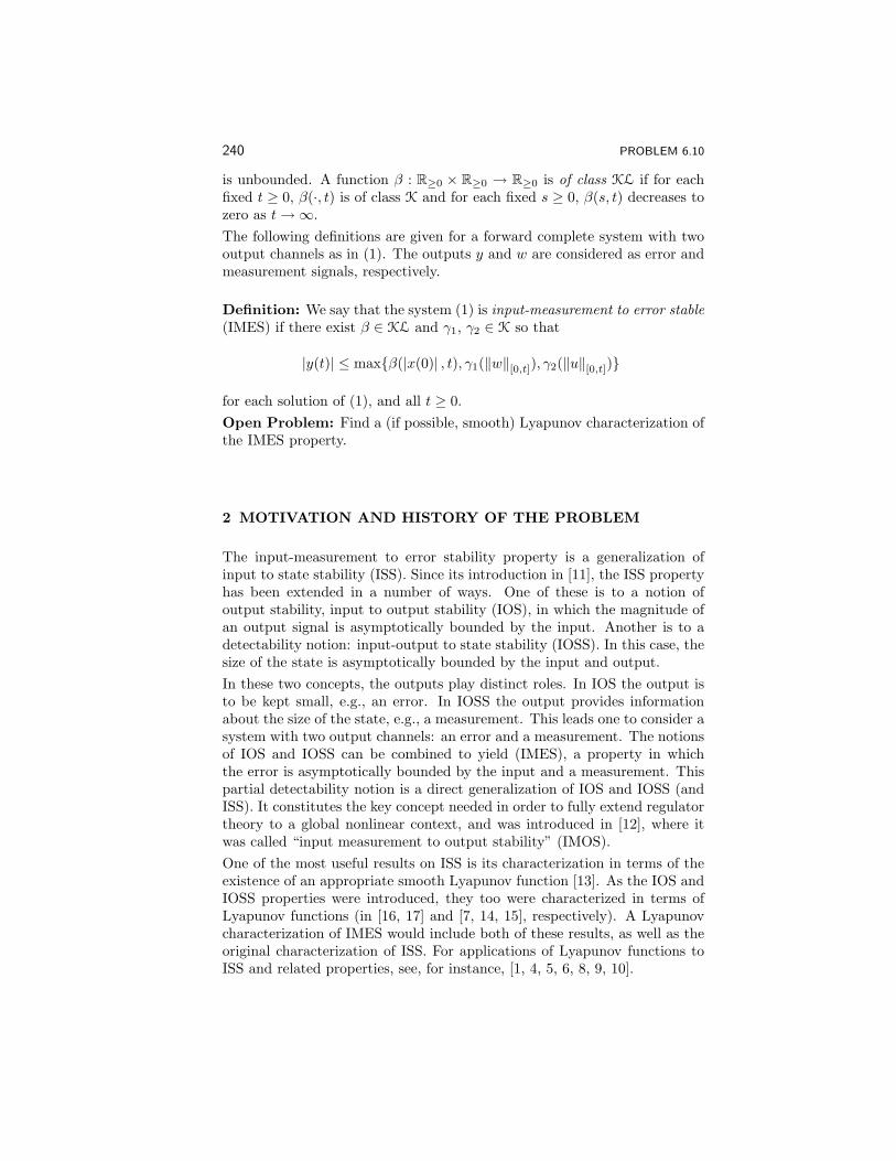
240 PROBLEM 6.10
is unbounded. A function β : R≥0 × R≥0 → R≥0 is of class KL if for eachfixed t ≥ 0, β(·, t) is of class K and for each fixed s ≥ 0, β(s, t) decreases tozero as t→∞.The following definitions are given for a forward complete system with twooutput channels as in (1). The outputs y and w are considered as error andmeasurement signals, respectively.
Definition: We say that the system (1) is input-measurement to error stable(IMES) if there exist β ∈ KL and γ1, γ2 ∈ K so that
|y(t)| ≤ maxβ(|x(0)| , t), γ1(‖w‖[0,t]), γ2(‖u‖[0,t])
for each solution of (1), and all t ≥ 0.Open Problem: Find a (if possible, smooth) Lyapunov characterization ofthe IMES property.
2 MOTIVATION AND HISTORY OF THE PROBLEM
The input-measurement to error stability property is a generalization ofinput to state stability (ISS). Since its introduction in [11], the ISS propertyhas been extended in a number of ways. One of these is to a notion ofoutput stability, input to output stability (IOS), in which the magnitude ofan output signal is asymptotically bounded by the input. Another is to adetectability notion: input-output to state stability (IOSS). In this case, thesize of the state is asymptotically bounded by the input and output.In these two concepts, the outputs play distinct roles. In IOS the output isto be kept small, e.g., an error. In IOSS the output provides informationabout the size of the state, e.g., a measurement. This leads one to consider asystem with two output channels: an error and a measurement. The notionsof IOS and IOSS can be combined to yield (IMES), a property in whichthe error is asymptotically bounded by the input and a measurement. Thispartial detectability notion is a direct generalization of IOS and IOSS (andISS). It constitutes the key concept needed in order to fully extend regulatortheory to a global nonlinear context, and was introduced in [12], where itwas called “input measurement to output stability” (IMOS).One of the most useful results on ISS is its characterization in terms of theexistence of an appropriate smooth Lyapunov function [13]. As the IOS andIOSS properties were introduced, they too were characterized in terms ofLyapunov functions (in [16, 17] and [7, 14, 15], respectively). A Lyapunovcharacterization of IMES would include both of these results, as well as theoriginal characterization of ISS. For applications of Lyapunov functions toISS and related properties, see, for instance, [1, 4, 5, 6, 8, 9, 10].
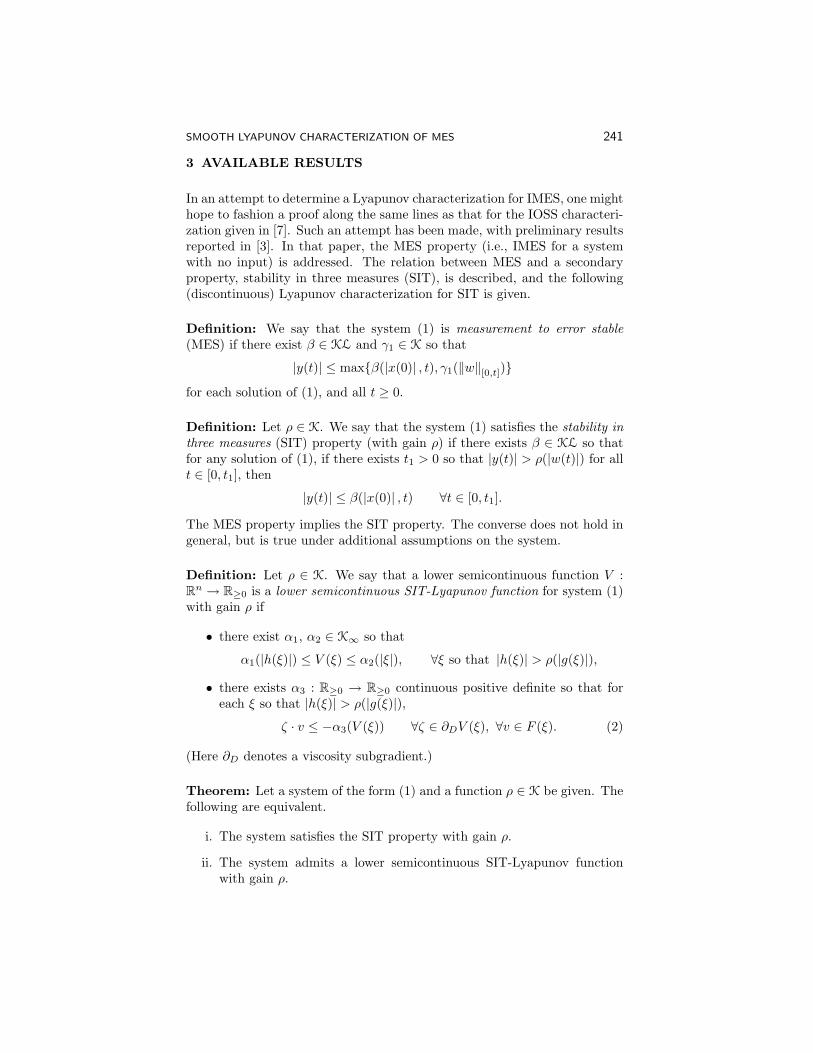
SMOOTH LYAPUNOV CHARACTERIZATION OF MES 241
3 AVAILABLE RESULTS
In an attempt to determine a Lyapunov characterization for IMES, one mighthope to fashion a proof along the same lines as that for the IOSS characteri-zation given in [7]. Such an attempt has been made, with preliminary resultsreported in [3]. In that paper, the MES property (i.e., IMES for a systemwith no input) is addressed. The relation between MES and a secondaryproperty, stability in three measures (SIT), is described, and the following(discontinuous) Lyapunov characterization for SIT is given.
Definition: We say that the system (1) is measurement to error stable(MES) if there exist β ∈ KL and γ1 ∈ K so that
|y(t)| ≤ maxβ(|x(0)| , t), γ1(‖w‖[0,t])
for each solution of (1), and all t ≥ 0.
Definition: Let ρ ∈ K. We say that the system (1) satisfies the stability inthree measures (SIT) property (with gain ρ) if there exists β ∈ KL so thatfor any solution of (1), if there exists t1 > 0 so that |y(t)| > ρ(|w(t)|) for allt ∈ [0, t1], then
|y(t)| ≤ β(|x(0)| , t) ∀t ∈ [0, t1].
The MES property implies the SIT property. The converse does not hold ingeneral, but is true under additional assumptions on the system.
Definition: Let ρ ∈ K. We say that a lower semicontinuous function V :Rn → R≥0 is a lower semicontinuous SIT-Lyapunov function for system (1)with gain ρ if
• there exist α1, α2 ∈ K∞ so that
α1(|h(ξ)|) ≤ V (ξ) ≤ α2(|ξ|), ∀ξ so that |h(ξ)| > ρ(|g(ξ)|),
• there exists α3 : R≥0 → R≥0 continuous positive definite so that foreach ξ so that |h(ξ)| > ρ(|g(ξ)|),
ζ · v ≤ −α3(V (ξ)) ∀ζ ∈ ∂DV (ξ), ∀v ∈ F (ξ). (2)
(Here ∂D denotes a viscosity subgradient.)
Theorem: Let a system of the form (1) and a function ρ ∈ K be given. Thefollowing are equivalent.
i. The system satisfies the SIT property with gain ρ.
ii. The system admits a lower semicontinuous SIT-Lyapunov functionwith gain ρ.
242 PROBLEM 6.10
iii. The system admits a lower semicontinuous exponential decay SIT-Lyapunov function with gain ρ.
Further details are available in [3] and [2].
BIBLIOGRAPHY
[1] R. A. Freeman and P. V. Kokotovi’c, Robust Nonlinear Control Design,State-Space and Lyapunov Techniques, Birkhauser, Boston, 1996.
[2] B. Ingalls, Comparisons of Notions of Stability for Nonlinear ControlSystems with Outputs, Ph.D. thesis, Rutgers University, New Brunswick,New Jersey, USA, 2001. Available at www.cds.caltech.edu/∼ingalls.
[3] B. Ingalls, E. D. Sontag, and Y. Wang, “Measurement to error stability:a notion of partial detectability for nonlinear systems,” submitted.
[4] A. Isidori, Nonlinear Control Systems II, Springer-Verlag, London, 1999.
[5] H. K. Khalil, Nonlinear Systems, Second Edition, Prentice-Hall, UpperSaddle River, NJ, 1996.
[6] P. Kokotovic and M. Arcak, “Constructive nonlinear control: Progressin the 90s,” Invited Plenary Talk, IFAC Congress, In: Proc. 14th IFACWorld Congress, the Plenary and Index Volume, pp. 49–77, Beijing, 1999.
[7] M. Krichman, E. D. Sontag, and Y. Wang, “Input-output-to-state stabil-ity,” SIAM Journal on Control and Optimization 39, 2001, pp. 1874-1928,2001.
[8] M. Krstic and H. Deng, Stabilization of Uncertain Nonlinear Systems,Springer-Verlag, London, 1998.
[9] M. Krstic, I. Kanellakopoulos, and P. V. Kokotovic, Nonlinear and Adap-tive Control Design, John Wiley & Sons, New York, 1995.
[10] R. Sepulchre, M. Jankovic, P. V. Kokotovic, Constructive NonlinearControl, Springer, 1997.
[11] E. D. Sontag, “Smooth stabilization implies coprime factorization,”IEEE Transactions on Automatic Control 34, 1989, pp. 435–443.
[12] E. D. Sontag, “The ISS philosophy as a unifying framework for stability-like behavior,” In: Nonlinear Control in the Year 2000 (Volume 2) (Lec-ture Notes in Control and Information Sciences, A. Isidori, F. Lamnabhi-Lagarrigue, and W. Respondek, eds.), Springer-Verlag, Berlin, 2000, pp.443-468.
SMOOTH LYAPUNOV CHARACTERIZATION OF MES 243
[13] E. D. Sontag and Y. Wang, “On characterizations of the input-to-statestability property,” Systems & Control Letters 24, pp. 351–359, 1995.
[14] E. D. Sontag and Y. Wang, “Detectability of nonlinear systems,” In:Proceedings of the Conference on Information Sciences and Systems(CISS 96), Princeton, NJ, 1996, pp. 1031–1036.
[15] E. D. Sontag and Y. Wang, “Output-to-state stability and detectabilityof nonlinear systems,” Systems & Control Letters 29, pp. 279–290, 1997.
[16] E. D. Sontag and Y. Wang, “Notions of input to output stability,”Systems & Control Letters 38, pp. 351–359, 1999.
[17] E. D. Sontag and Y. Wang, “Lyapunov characterizations of input to out-put stability,” SIAM Journal on Control and Optimization 39, pp. 226–249, 2001.


PART 7
Controllability, Observability

Problem 7.1
Time for local controllability of a 1-D tank containing
a fluid modeled by the shallow water equations
Jean-Michel CoronUniversite Paris-SudDepartement de MathematiqueBatiment 42591405 [email protected]
1 DESCRIPTION OF THE PROBLEM
We consider a 1-D tank containing an inviscid incompressible irrotationalfluid. The tank is subject to one-dimensional horizontal moves. We assumethat the horizontal acceleration of the tank is small compared to the gravityconstant and that the height of the fluid is small compared to the lengthof the tank. This motivates the use of the Saint-Venant equations [5] (alsocalled shallow water equations) to describe the motion of the fluid; see, e.g.,[2, Sec. 4.2]. After suitable scaling arguments, the length of the tank and thegravity constant can be taken to be equal to 1; see [1]. Then the dynamicsequations considered are, see [3] and [1],
Ht (t, x) + (Hv)x (t, x) = 0, (1)
vt (t, x) +(H +
v2
2
)x
(t, x) = −u (t) , (2)
v(t, 0) = v(t, 1) = 0, (3)dsdt
(t) = u (t) , (4)
dDdt
(t) = s (t) , (5)
where
• H (t, x) is the height of the fluid at time t and for x ∈ [0, 1],
• v (t, x) is the horizontal water velocity of the fluid in a referential at-tached to the tank at time t and for x ∈ [0, 1] (in the shallow water
248 PROBLEM 7.1
model, all the points on the same vertical have the same horizontalvelocity),
• u is the horizontal acceleration of the tank in the absolute referential,
• s is the horizontal velocity of the tank,
• D is the horizontal displacement of the tank.
This is a control system, denoted Σ, where
• the state is Y = (H, v, s,D),
• the control is u ∈ R.
Still, by scaling arguments, we may assume that, for every steady state, H,which is then a constant function, is equal to 1; see [1]. One is interestedin the local controllability of the control system Σ around the equilibriumpoint
(Ye, ue) := ((1, 0, 0, 0), 0).
Of course, the total mass of the fluid is conserved so that, for every solutionof (1) to (3),
ddt
∫ 1
0
H (t, x) dx = 0. (6)
One gets (6) by integrating (1) on [0, 1] and by using (3 together with anintegration by parts.) Moreover, if H and v are of class C1, it follows from(2) and (3) that
Hx(t, 0) = Hx(t, 1) (= −u (t)). (7)
Therefore we introduce the vector space E of functions Y = (H, v, s,D) ∈C1([0, 1])× C1([0, 1])× R× R such that
Hx(0) = Hx(1), (8)v(0) = v(1) = 0, (9)
and consider the affine subspace Y ⊂ E of Y = (H, v, s,D) ∈ E satisfying∫ 1
0
H(x)dx = 1. (10)
With these notations, we can define a trajectory of the control system Σ.Definition of a trajectory: Let T1 and T2 be two real numbers satisfyingT1 6 T2. A function (Y, u) = ((H, v, s,D), u) : [T1, T2] → Y × R is atrajectory of the control system Σ if
(i) the functions H and v are of class C1 on [T1, T2]× [0, 1],
TIME FOR LOCAL CONTROLLABILITY OF A 1-D TANK 249
(ii) the functions s and D are of class C1 on [T1, T2] and the function u iscontinuous on [0, T ],
(iii) the equations (1) to (5) hold for every (t, x) ∈ [T1, T2]× [0, 1].
For w ∈ C1([0, 1]), let
|w|1 := Max|w(x)|+ |wx(x)|; x ∈ [0, 1].
We now consider the following property of local controllability of Σ around(Ye, ue).Definition of P(T ): Let T > 0. The control system Σ satisfies the prop-erty P(T ) if, for every ε, there exists η > 0 such that, for every Y0 =(H0, v0, s0, D0) ∈ Y, and for every Y1 = (H1, v1, s1, D1) ∈ Y such that
|H0 − 1|1 + |v0|1 + |H1 − 1|1 + |v1|1 + |s0|+ |s1|+ |D0|+ |D1| < η,
there exists a trajectory
(Y, u) : [0, T ] → Y× R, t 7→ ((H (t) , v (t) , s (t) , D (t)) , u (t))
of the control system Σ such that
Y (0) = Y0 and Y (T ) = Y1, (11)
and, for every t ∈ [0, T ],
|H (t)− 1|1 + |v (t)|1 + |s (t)|+ |D (t)|+ |u (t)| < ε. (12)
Our open problem is to find for which T > 0 P(T ) holds. We conjecturethat P(T ) holds if and only if T > 2.
2 MOTIVATION AND HISTORY OF THE PROBLEM
The problem of controllability of the system Σ has been raised by F. Dubois,N. Petit, and P. Rouchon in [3]. Let us recall that they have studied in thispaper the controllability of the linearized control system around (Ye, ue).This linearized control system is
(Σ0)
ht + vx = 0,vt + hx = −u (t) ,v(t, 0) = v(t, 1) = 0,dsdt (t) = u (t) ,dDdt (t) = s (t) ,
(13)
where the state is (h, v, s,D) ∈ Y0, with
Y0 :=
(h, v, s,D) ∈ E;∫ 1
0
hdx = 0,
and the control is u ∈ R. It is proved in [3] that Σ0 is not control-lable. It is also proved in [3] that, even if Σ0 is not controllable, for any
250 PROBLEM 7.1
T > 1, one can move during the interval of time [0, T ] from any steadystate (h0, v0, s0, D0) := (0, 0, 0, D0) to any steady state (h1, v1, s1, D1) :=(0, 0, 0, D1) for the linear control system Σ0; see also [4] when the tank hasa nonstraight bottom. Unfortunately, this does not imply that the relatedproperty (move from (H0, v0, s0, D0) := (0, 0, 0, D0) to (H1, v1, s1, D1) :=(0, 0, 0, D1) also holds for the nonlinear control system Σ, even if |D1 −D0|is arbitrary small but not 0. In fact we conjecture that, for ε > 0 smallenough, even if |D1 −D0| is arbitrarily small but not 0, one needs T > 2 tomove from (H0, v0, s0, D0) := (1, 0, 0, D0) to (H1, v1, s1, D1) := (1, 0, 0, D1)for the nonlinear control system Σ if one requires (12).
3 AVAILABLE RESULTS
Clearly, P(T ) implies P(T ′) for T ≤ T ′. Using the characteristics of thehyperbolic system (1)-(2), one easily sees that P(T ) does not hold T < 1. Itis proved in [1] that P(T ) holds for T large enough. The method used in [1]requires, at least, T > 2.
BIBLIOGRAPHY
[1] J.-M. Coron, “Local controllability of a 1-D tank containing a fluid mod-eled by the shallow water equations,” reprint University Paris-Sud, 2002,accepted for publication in ESAIM: COCV.
[2] L. Debnath, Nonlinear Water Waves, Academic Press, San Diego, 1994.
[3] F. Dubois, N. Petit, and P. Rouchon, “Motion planning and nonlinearsimulations for a tank containing a fluid,” ECC 99.
[4] N. Petit and P. Rouchon, “Dynamics and solutions to some control prob-lems for water-tank systems,” preprint, CIT-CDS 00-004, 2000, acceptedfor publication in IEEE Transactions on Automatic Control.
[5] A.J.C.B. de Saint-Venant, “Theorie du mouvement non permanent deseaux, avec applications aux crues des rivieres et a l’introduction desmarees dans leur lit,” C.R. Acad. Sci. Paris, 53 pp. 147-154, 1971.
Problem 7.2
A Hautus test for infinite-dimensional systems
Birgit JacobFachbereich MathematikUniversitat DortmundD-44221 [email protected]
Hans ZwartDepartment of Applied MathematicsUniversity of TwenteP.O. Box 217, 7500 AE EnschedeThe [email protected]
1 DESCRIPTION OF THE PROBLEM
We consider the abstract system
x(t) =Ax(t), x(0) = x0, t ≥ 0 (1)y(t) =Cx(t), t ≥ 0, (2)
on a Hilbert space H. Here A is the infinitesimal generator of an expo-nentially stable C0-semigroup (T (t))t≥0 and by the solution of (1) we meanx(t) = T (t)x0, which is the weak solution. If C is a bounded linear oper-ator from H to a second Hilbert space Y , then it is straightforward to seethat y(·) in (2) is well-defined and continuous. However, in many PDE’s,rewritten in the form (1)-(2), C is only a bounded operator from D(A) toY (D(A) denotes the domain of A), although the output is a well-defined(locally) square integrable function. In the following, C will always be abounded operator from D(A) to Y . Note that D(A) is a dense subset ofH. If the output is locally square integrable, then C is called an admissibleobservation operator, see Weiss [11]. It is not hard to see that since the C0-semigroup is exponentially stable, the output is locally square integrable ifand only if it is square integrable. Using the uniform boundedness theorem,we see that the observation operator C is admissible if and only if there
252 PROBLEM 7.2
exists a constant L > 0 such that∫ ∞
0
‖CT (t)x‖2Y dt ≤ L‖x‖2H , x ∈ D(A). (3)
Assuming that the observation operator C is admissible, system (1)-(2) issaid to be exactly observable if there is a bounded mapping from the outputtrajectory to the initial condition, i.e., there exists a constant l > 0 suchthat ∫ ∞
0
‖CT (t)x‖2Y dt ≥ l‖x‖2H , x ∈ D(A). (4)
Often the emphasis is on exact observability on a finite interval, which meansthat the integral in (4) is over [0, t0] for some t0 > 0. However, for exponen-tially stable semigroups, both notions are equivalent, i.e., if (4) holds andthe system is exponentially stable, then there exists a t0 > 0 such that thesystem is exactly observable on [0, t0].There is a strong need for easy verifiable equivalent conditions for exact ob-servability. Based on the observability conjecture by Russell and Weiss [9]we now conjecture the following:
Conjecture Let A be the infinitesimal generator of an exponentially stableC0-semigroup on a Hilbert space H and let C be an admissible observationoperator. Then system (1)-(2) is exactly observable if and only if
(C1) (T (t))t≥0 is similar to a contraction, i.e., there exists a bounded oper-ator S from H to H, which is boundedly invertible such that(ST (t)S−1)t≥0 is a contraction semigroup; and
(C2) there exists a m > 0 such that
‖(sI −A)x‖2H + |Re(s)|‖Cx‖2Y ≥ m|Re(s)|2‖x‖2H (5)
for all complex s with negative real part, and for all x ∈ D(A).
Our conjecture is a revised version of the (false) conjecture by Russell andWeiss; they did not require that the semigroup is similar to a contraction.
2 MOTIVATION AND HISTORY OF THE CONJECTURE
System (1)-(2) with A ∈ Cn×n and C ∈ Cp×n is observable if and only if
ranksI −AC
= n for all s ∈ C. (6)
This is known as the Hautus test, due to Hautus [2] and Popov [8]. If Ais a stable matrix, then (6) is equivalent to condition (C2). Although thereare some generalizations of the Hautus test to delay differential equations
A HAUTUS TEST FOR INFINITE-DIMENSIONAL SYSTEMS 253
(see, e.g., Klamka [6] and the references therein) the full generalization of theHautus test to infinite-dimensional linear systems is still an open problem.It is not hard to see that if (1)-(2) is exactly observable, then the semigroupis similar to a contraction, see Grabowski and Callier [1] and Levan [7].Condition (C2) was found by Russell and Weiss [9]: they showed that thiscondition is necessary for exact observability, and, under the extra assump-tion that A is bounded, they showed that this condition also is sufficient.Without the explicit usage of condition (C1) it was shown that condition(C2) implies exact observability if
• A has a Riesz basis of eigenfunctions, Re(λn) = −ρ1, |λn+1−λn| > ρ2,where λn are the eigenvalues of A, and ρ1, ρ2 > 0, [9]; or if
• m in equation (5) is one, [1]; or if
• A is skew-adjoint and C is bounded, Zhou and Yamamoto [12]; or if
• A has a Riesz basis of eigenfunctions, and Y = Cp, Jacob and Zwart[5].
Recently, we showed that (C2) is not sufficient in general, [4]. The C0-semigroup in our counterexample is an analytic semigroup, which is notsimilar to a contraction semigroup. The output space in the example is justthe complex plane C.
3 AVAILABLE RESULTS AND CLOSING REMARKS
In order to prove the conjecture it is sufficient to show that for exponentiallystable contraction semigroups condition (C2) implies exact observability.It is well-known that system (1)-(2) is exactly observable if and only if thereexists a bounded operator L that is positive and boundedly invertible andsatisfies the Lyapunov equation
〈Ax1, Lx2〉H + 〈Lx1, Ax2〉H = 〈Cx1, Cx2〉Y , for all x1, x2 ∈ D(A). (7)
From the admissibility of C and the exponential stability of the semigroup,one easily obtains that equation (7) has a unique (non-negative) solution.Russell and Weiss [9] showed that Condition (C2) implies that this solutionhas zero kernel. Thus the Lyapunov equation (2) could be a starting pointfor a proof of the conjecture.We have stated our conjecture for infinite-dimensional output spaces. How-ever, it could be that it only holds for finite-dimensional output spaces.If the output space Y is one-dimensional one could try to prove the conjectureusing powerful tools like the Sz.-Nagy-Foias model theorem (see [10]). Thistool was quite useful in the context of admissibility conditions for contraction
254 PROBLEM 7.2
semigroups [3]. Based on this observation, it would be of great interest tocheck our conjecture for the right shift semigroup on L2(0,∞).We believe that exponential stability is not essential in our conjecture, andcan be replaced by strong stability and infinite-time admissibility, see [5].Note that our conjecture is also related to the left-invertibility of semigroups,see [1] and [4] for more details.
BIBLIOGRAPHY
[1] P. Grabowski and F. M. Callier, “Admissible observation operators,semigroup criteria of admissibility,” Integral Equation and OperatorTheory, 25:182–198, 1996.
[2] M. L. J. Hautus, “Controllability and observability conditions for lin-ear autonomous systems,” Ned. Akad. Wetenschappen, Proc. Ser. A,72:443–448, 1969.
[3] B. Jacob and J. R. Partington, “The Weiss conjecture on admissibilityof observation operators for contraction semigroups,” Integral Equationsand Operator Theory, 40(2):231-243, 2001.
[4] B. Jacob and H. Zwart, “Disproof of two conjectures ofGeorge Weiss,” Memorandum 1546, Faculty of Mathemat-ical Sciences, University of Twente, 2000. Available athttp://www.math.utwente.nl/publications/
[5] B. Jacob and H. Zwart, “Exact observability of diagonal systemswith a finite-dimensional output operator,” Systems & Control Letters,43(2):101-109, 2001.
[6] J. Klamka, Controllability of Dynamical Systems, Kluwer AcademicPublisher, 1991.
[7] N. Levan, “The left-shift semigroup approach to stability of distributedsystems,” J. Math. Ana. Appl., 152: 354–367, 1990.
[8] V. M. Popov, Hyperstability of Control Systems. Editura Academiei,Bucharest, 1966 (in Romanian); English trans. by Springer Verlag,Berlin, 1973.
[9] D. L. Russell and G. Weiss, “A general necessary condition for exactobservability,” SIAM J. Control Optim., 32(1):1–23, 1994.
[10] B. Sz.-Nagy and C. Foias, Harmonic analysis of operators on Hilbertspaces, Amsterdam-London: North-Holland Publishing Company. XIII,1970.
A HAUTUS TEST FOR INFINITE-DIMENSIONAL SYSTEMS 255
[11] G. Weiss, “Admissible observation operators for linear semigroups,”Israel Journal of Mathematics, 65:17–43, 1989.
[12] Q. Zhou and M. Yamamoto, “Hautus condition on the exact controlla-bility of conservative systems,” Int. J. Control, 67(3):371–379, 1997.

Problem 7.3
Three problems in the field of observability
Philippe JouanLaboratoire R. SalemCNRS UMR 6085Universite de RouenMathematiques, site Colbert76821 Mont-Saint-Aignan [email protected]
1 INTRODUCTION.
Let X be a C∞ (resp. Cω), connected manifold. We consider on X thesystem
Σ =x = f(x, u)y = h(x) (1)
where x ∈ X, u ∈ U = [0, 1]m, and y ∈ Rp. The parametrized vector fieldf and the output function h are assumed to be C∞ (resp. Cω). In order toavoid certain complications, the state space X is assumed to be compact, butthis assumption is not crucial (we can for instance assume that the vectorfield f vanishes out of a relatively compact open subset of X).The three problems addressed herein concern observability and the existenceof observers for such systems.
2 PROBLEM 1.
We first consider an uncontrolled system:
Σu =x = f(x)y = h(x). (2)
This system is assumed to be observable (in the following sense: the tra-jectories starting from two different initial states are distinguished by theoutput).

THREE PROBLEMS IN THE FIELD OF OBSERVABILITY 257
Whenever the nth derivative of the output with respect to the vector field fis a Cr-function of the output and the n − 1 previous ones it is possible toconstruct obververs (see [5], [9]). More accurately, the injective mapping
Φ = (h, Lfh, L2fh, . . . , L
n−1f h)
is used to “immerse” Σu into Rpn where a Cr-observer is designed. The ob-served data are the outputs of Σu together with their (n− 1)th first deriva-tives. The state of the system, being a continuous mapping of(h, Lfh, L2
fh, . . . , Ln−1f h), is thus estimated by the observer.
More generaly a Cr-observer for Σu is a system Σ defined in an open subsetV of Rn by
Σ =z = F (z, y)x = θ(z) (3)
where F is a Cr-vector field on V and θ is a continuous mapping from Vinto X such that
∀x ∈ X, ∀z ∈ V limt7→+∞
d(x(t), x(t)) = 0
for any distance d on X compatible with the topology of X.The first problem is:Does the existence of a Cr-observer for Σu imply the existence of an integern such that the nth derivative of the output is a Cr-function of the outputand the n−1 previous ones? In an equivalent way does it exist a Cr-functionϕ such that
Lnfh = ϕ(h, Lfh, L2fh, . . . , L
n−1f h) ?
A positive answer to this question would imply that all the observabilityproperties of an uncontrolled system are contained in the functional relation
Lnfh = ϕ(h, Lfh, L2fh, . . . , L
n−1f h).
Notice that we already know that the kind of dependence between the nth
derivative of the output and the preceding ones, that is the kind of functionϕ, determines whether the system is linearizable, or linearizable modulo anoutput injection (see [2], [7]).
3 PROBLEM 2.
Once we know that a controlled system is observable in the weak sense of[4] (two different initial states have to be distinguished by the output forat least one input) a question arises naturally: which inputs are universal?(An input is universal if any two different initial states are distinguished bythe output for this input, see [8].) An equivalent formulation is: for whichinputs is the system observable?
258 PROBLEM 7.3
For generic reasons, we consider controlled systems with more outputs thaninputs: p > m.Problem 2 is:Is it true that the set of C∞-systems (resp. Cω-systems) that are observablefor every C∞ input contains an open (or better an open and dense) subsetof the set of C∞-systems (resp. the set of Cω-systems)? Both in the C∞ andCω cases does observability for every C∞-input imply observability for everyL∞-input?The following facts are known:
i. The set of systems observable for every C∞-input is dense in the set ofC∞ or Cω-systems (see [3], [1]).
ii. For a given bound, the set of systems observable for every C∞- inputwhose 2 dim(X) first derivatives are bounded contains an open anddense subset of the set of C∞ or Cω-systems (see [3], [1]).
iii. A Cω-system observable for every C∞-input is observable for everyL∞-input (see [3]).
iv. In the single-input, control-affine, C∞-case, the implication
Σ C∞-observable =⇒ Σ L∞-observable
is true for an open and dense subset of systems (see [6]).
Of course, a positive answer to this problem would mean that the property ofbeing observable for every L∞-input is preserved under slight perturbations.
4 PROBLEM 3.
Since the set of systems observable for every L∞-input is residual (withmore ouputs than inputs), it is very interesting to design observers for them,particularly if this set contains an open subset.At the present time, the more general construction of observers for nonlinearsystems is the high gain one (see [3]). But the observers designed in thisway have the default to make use of the derivatives of the input and cannotwork if this last is only L∞. In some particular cases (linearizable systems,linearizable modulo an output injection systems, bilinear systems, uniformlyobservable systems . . . ) observers that works for every input are known butthey cannot be generalized.Problem 3 is therefore:For systems observable for every L∞-input, find a general construction ofan observer which works for every L∞-input.Notice that if the system is “immersed” in RN (in a sense to make precise)the “immersion” must not depend on the input: in that case the image of
THREE PROBLEMS IN THE FIELD OF OBSERVABILITY 259
the vector field f in RN would depend upon the derivative of the input. Inparticular the mapping
Φ = (h, Lfh, L2fh, . . . , L
n−1f h)
from X into Rpn cannot be used because the vector field f(x, u) dependsupon u and so are Lfh(x, u), L2
fh(x, u), . . ., Ln−1f h(x, u).
BIBLIOGRAPHY
[1] M. Balde and Ph. Jouan, “Genericity of observability of control-affinesystems,” Control Optimization and Calculus of Variations, vol. 3, 1998,345-359.
[2] M. Fliess and I. Kupka, “A finiteness criterion for nonlinear input-output differential systems,” SIAM J. on Control and Optimization,21 (1983), 5, 721-728.
[3] J. P. Gauthier and I. Kupka, Deterministic Observation Theory andApplications, Cambridge University Press, 2001.
[4] R. Hermann and A. J. Krener, “Nonlinear controllability and observ-ability,” IEEE Trans. Aut. Contro, AC-22 (1977), 728-740.
[5] Ph. Jouan and J. P. Gauthier, “Finite singularities of nonlinear systems.Output stabilization, observability and observers,” Journal of Dynam-ical and Control Systems, vol.2, no 2, 1996, 255-288.
[6] Ph. Jouan, “C∞ and L∞ observability of single-input C∞-Systems,”Journal of Dynamical and Control Systems, vol. 7, no 2, 2001, 151-169.
[7] Ph. Jouan, “Immersion of nonlinear systems into linear systems modulooutput injection,” submitted to SIAM J. on Control and Optimization.
[8] H. J. Sussmann, “Single-input observability of continuous-time sys-tems,” Math. Syst. Theory 12 (1979), 371-393.
[9] X. Xia and M. Zeitz, “On nonlinear continuous observers,” Int. J. Con-trol, vol. 66, no 6, 1997, 943-954.
Problem 7.4
Control of the KdV equation
Lionel RosierInstitut Elie CartanUniversite Henri Poincare Nancy 1B.P. 23954506 Vandœuvre-les-Nancy [email protected]
1 DESCRIPTION OF THE PROBLEM
The Korteweg-de Vries (KdV) equation is the simplest model for unidirec-tional propagation of small amplitude long waves in nonlinear dispersivesystems. It occurs in various physical contexts (e.g., water waves, plasmaphysics, nonlinear optics). It reads
yt + yxxx + yx + y yx = 0, t > 0, x ∈ Ω, (1)
the subscripts denoting partial derivatives (e.g., yt = ∂y∂t ). The KdV equa-
tion has been intensively studied since the 1960s because of its fascinatingproperties (infinite set of conserved integral quantities, integrability, Katosmoothing effect, etc.). (See [5] and the references therein.)Here, we are concerned with the boundary controllability of the KdV equa-tion in the domain Ω = (0,+∞). For any pair (a, b) with 0 ≤ a < b ≤ +∞let C∞0 (a, b) denote the space of functions of class C∞ and with compactsupport in (a, b). Given T > 0, y0 ∈ C∞0 (0,+∞) and h ∈ C∞0 (0, T ), it is bynow well known (see [1]) that the initial-boundary-value problem yt + yxxx + yx + yyx = 0, 0 < t < T, 0 < x < +∞
y(t, 0) = h(t), 0 < t < Ty(0, x) = y0(x), 0 < x < +∞
(2)
admits a unique classical solution that is smooth. The boundary value h isthe input of the system. Let R(y0, T ) denote the space of all reachable statesfrom y0 in time T ; that is,
R(y0, T ) = y(T, .); y fulfills (2) for some h ∈ C∞0 (0, T ). (3)
CONTROL OF THE KDV EQUATION 261
We are now in a position to state the problem of interest.
Open Problem: Is is true that 0 ∈ R(y0, T ) for T is large enough ?
The main difficulty of the problem is that the domain is unbounded. Noticethat it would also be of great interest to identify the closure of R(y0, T ) inL2(0,+∞).
2 MOTIVATION AND HISTORY OF THE PROBLEM
The KdV equation has been first introduced in [4] to explain the emergenceof long solitary waves, the so-called “solitons.” In this context, t stands forthe elapsed time, x is the independent space variable, and y = y(t, x) standsfor the deviation of the fluid surface from the rest position. The above controlproblem may serve as a model for the control of the fluid surface in a shallowcanal by means of a wavemaker. Indeed, taking Lagrangian coordinates, itis proved in [10] that the movement of the fluid surface is governed by (2),the speed of the moving boundary being roughly represented by the input h.Thus, the space R(0, T ) stands for the set of waves that may be generated(from the rest position) by the wavemaker in time T .A similar control problem is investigated in [7], but with a fluid model inwhich both the dispersive and nonlinear effects are neglected. In [2] theauthor uses the (nonlinear) shallow water equations as a fluid model toinvestigate the control of the fluid surface in a moving tank. These equationsare appropriate in situations where the dispersive effects may be neglected,e.g., when the height of the fluid and the length of the tank are of the sameorder of magnitude. The shallow water equations have to be replaced by theKdV equation (or the Boussinesq system) when studying the propagation oftraveling waves.The above problem is important for the following reason. A lack of compact-ness, due to the fact that the domain is unbounded, prevents us from usingthe standard linearization procedure in the study of the controllability prop-erties of (2). Therefore, a new approach (based on the inverse scattering?)has to be developed to investigate the (exact or approximate) controllabilityof the nonlinear KdV equation on the half line.
3 AVAILABLE RESULTS
The boundary controllability of the KdV equation has been investigated innumerous papers; see, e.g., [3], [8], [11] and [12]. In these papers, the do-main Ω = (0, L) is bounded and the control is applied at the right endpoint,although the waves are expected to move from the left to the right. If the
262 PROBLEM 7.4
control is applied at the left endpoint, and if the system is supplementedby the boundary conditions y = yx = 0 at x = L, then it is proved in [10]that for any T,L > 0, 0 ∈ R(y0, T ) for any initial state y0 with a smallenough H3(0, L)-norm. It means that a soliton moving to the right maybe caught up and annihilated by a set of waves generated by the wave-maker. This result rests on a Carleman estimate for the linearized equation(i.e., (1) without the nonlinear term yyx). When we look at the linearizedequation on the unbounded domain Ω = (0,+∞), then the controllabilityresults are not so good, due to a lack of compactness. Indeed, it is provedin [9] that there exists a state y0 ∈ L2(0,+∞) for which any trajectory con-necting y0 to the null state does not belong to L∞(0, T, L2(0,+∞)) (thatis, ess sup0<t<T
∫ +∞0
y(t, x)2 dx = +∞). It means that the bad behavior ofthe trajectory y(t, x) as x → +∞ is the price to be paid to get the null-controllability. (A similar phenomenon has been observed in [6] for the heatequation.) Thus, the linearization procedure fails since we do not have anybound on ‖y(t, .)‖L2(0,+∞).
BIBLIOGRAPHY
[1] J. Bona, R. Winther, “The Korteweg-de Vries equation, posed in aquarter-plane,” SIAM J. Math. Anal., 14, pp. 1056-1106, 1983.
[2] J.-M. Coron, “Local controllability of a 1-D tank containing a fluid mod-eled by the shallow water equations,” A tribute to J. L. Lions, ESAIMControl Optim. Calc. Var., 8, pp. 513-554, 2002 (electronic).
[3] E. Crepeau, “Exact boundary controllability of the Korteweg-de Vriesequation around a non-trivial stationary solution,” Internat. J. Control74, pp. 1096–1106, 2001.
[4] D. J. Korteweg and G. de Vries, “On the change of form of long wavesadvancing in a rectangular canal, and on a new type of long stationarywaves,” Philos. Mag., 39, pp. 422-443, 1995.
[5] C. E. Kenig, G. Ponce, and L. Vega, “The Cauchy problem for theKorteweg-de Vries equation in Sobolev spaces of negatives indices,” Dukemath J., 71, pp. 1-21, 1993.
[6] S. Micu, E. Zuazua, “On the lack of null-controllability of the heat equa-tion on the half space,” Portugal. Math., 58, pp. 1-24, 2001.
[7] S. Mottelet, “Controllability and stabilization of a canal with wave gen-erators,” SIAM J. Control Optim., 38, pp. 711-735, 2000.
[8] L. Rosier, “Exact boundary controllability for the Korteweg-de Vriesequation on a bounded domain,” ESAIM Control Optim. Calc. Var., 2,pp. 33-55, 1997.
CONTROL OF THE KDV EQUATION 263
[9] L. Rosier, “Exact boundary controllability for the linear Korteweg-deVries equation on the half-line,” SIAM J. Control Optim.:, 39, pp. 331-351, 2000.
[10] L. Rosier, “Control of the surface of a fluid by a wavemaker,” in prepa-ration.
[11] D. L. Russell, B. Y. Zhang, “Exact controllability and stabilizabilityof the Korteweg-de Vries equation,” Trans. Amer. Math. Soc., 348, pp.3643-3672, 1996.
[12] B. Y. Zhang, “Exact boundary controllability of the Korteweg-de Vriesequation,” SIAM J. Control Optim., 37, pp. 543-565, 1999.


PART 8
Robustness, Robust Control

Problem 8.1
H∞-norm approximation
A. C. AntoulasDepartment of Electrical and Computer EngineeringRice University6100 South Main StreetHouston, TX [email protected]
A. AstolfiDepartment of Electrical and Electronic EngineeringImperial CollegeExhibition RoadSW7 2BT, LondonUnited [email protected]
1 DESCRIPTION OF THE PROBLEM
Let RHm∞ be the (Hardy) space of real-rational scalar1 transfer functions
of order m, bounded on the imaginary axisand analytic into the right-halfcomplex plane. The optimal approximation problem in the H∞ norm canbe statedas follows.
(A?) (Optimal Approximation in the H∞ norm)Given G(s) ∈ RHN
∞ and an integer n < N find,2 if possible, A?(s) ∈RHn
∞ such that
A?(s) = arg minA(s)∈RHn∞‖G(s)−A(s)‖∞. (1)
For such a problem, let
γ?n = minA(s)∈RHn∞‖G(s)−A(s)‖∞,
then two further problems can be posed.
1Similar considerations can be done for the nonscalar case.2By find we mean find an exact solution or an algorithm converging to the exact
solution.
268 PROBLEM 8.1
(D) (Optimal Distance problem in the H∞ norm)Given G(s) ∈ RHN
∞ and an integer n < N find γ?n.
(A) (Sub-optimal Approximation in the H∞ norm)Given G(s) ∈ RHN
∞, an integer n < N and γ > γ?n find A(s) ∈ RHn∞
such that
γ?n ≤ ‖G(s)− A(s)‖∞ ≤ γ.
The optimal H∞ approximation problem can be formally posed as a con-strained min-max problem. For, note that any function in RHn
∞ can be putin a one-to-one correspondence with a point θ of some (open) set Ω ⊂ R2n,therefore the problem of computing γ?ncan be posed as
γ?n = minθ∈Ω
maxω∈R
‖G(jω)−A(jω)‖, (2)
where A(s) = A(s, θ). The above formulation provides a brute force ap-proach to the solution of the problem. Unfortunately, this method is notof any use in general, because of the complexity of the set Ω and becauseof the curse of dimensionality. However, the formulation (2) suggests thatpossible candidate solutions of the optimal approximation problem are thesaddle points of the function
‖G(jω)−A(jω, θ)‖,
which can be, in principle, computed using numerical tools. It would beinteresting to prove (or disprove) that
minθ∈Ω
maxω∈R
‖G(jω)−A(jω, θ)‖ = maxω∈R
minθ∈Ω
‖G(jω)−A(jω, θ)‖.
The solution method based on the computation of saddle points does notgive any insight into the problem, neither exposes any systems theoreticinterpretation of the optimal approximant. An interesting property of theoptimal approximant is stated in the following simple fact, which can beused to rule out that a candidate approximant is optimal.
Fact: Let A?(s) ∈ RHn∞ be such that equation (1) holds. Suppose
|W (jω?)−A?(jω?)| = γ?n, (3)
and
A(jω?) 6= 0 (4)
for ω? = 0. Then there exists a constant ω 6= ω? such that
|W (jω)−A?(jω)| = γ?n,
i.e., if the value γ?n is attained by the function |W (jω)−A?(jω)|at ω = 0 itis also attained at some ω 6= 0.
Proof: We prove the statement by contradiction. Suppose
|W (jω)−A?(jω)| < γ?n, (5)

H∞-NORM APPROXIMATION 269
for all ω 6= ω? and consider the approximant A(s) = (1 + λ)A?(s), withλ ∈ IR. By equation (5), condition (4) and by continuity with respect to λand ω of
|W (jω)− A(jω)|,there is a λ? (sufficiently small) such that
maxω|W (jω)− (1 + λ?)A?(jω)| < γ?n,
or, what is the same, it is possible to obtain an approximant that is betterthan A?(s), hence a contradiction. /
It would be interesting to show that the above fact holds (or it does nothold) when ω? 6= 0.
2 AVAILABLE RESULTS AND POSSIBLE SOLUTION PATHS
Approximation and model reduction have always been central issues in sys-tem theory. For a recent survey on model reduction in the large-scale setting,we refer the reader to [1]. There are several results in this area. If the ap-proximation is performed in the Hankel norm, then an explicit solution of theoptimal approximation and model reduction problems has been given in [3].Note that this procedure provides, as a byproduct, an upper bound for γ?nand a solution of the suboptimal approximation problem. If the approxima-tion is performed in the H2 norm, several results and numerical algorithmsare available [4]. For approximation in the H∞ norm a conceptual solutionis given in [5]. Therein it is shown that the H∞ approximation problem canbe reduced to a Hankel norm approximation problem for an extended system(i.e., a system obtained from a state space realization of the original transferfunction G(s) by adding inputs and outputs). The extended system has tobe constructed with the constraint that the corresponding Grammians Pand Q satisfy
λmin(PQ) = (γ?n)2 with multiplicity N − n. (6)
However, the above procedure, as also noted by the authors of [5], is not com-putationally viable, and presupposes the knowledge of γ?n. Hence the needfor further study of the problem. In the recent paper [2], the decay ratesof the Hankel singular values of stable, single-input single-output systems,are studied. Let G(s) = p(s)
q(s) be the transfer function under consideration.The decay rate of the Hankel singular values is studied by introducing a newset of input/output system invariants, namely the quantities p(s)
q∗(s) , whereq(s)∗ = q(−s), evaluated at the poles of G(s). These results are expectedto yield light into the structure of the above problem (6). Another paperof interest especially for the suboptimal approximation case, is [6]. In thispaper the set, of all systems whose H∞ norm is less than some positivenumber γ is parameterized. Thus the following problem can be posed: given
270 PROBLEM 8.1
such a system with H∞ norm less than γ, find conditions under which itcan be decomposed in the sum of two systems, one of which is prespecified.Finally, there are two special classes of systems that may be studied to im-prove our insight into the general problem. The first class is composed ofsingle-input single-output discrete-time stable systems. For such systems,an interesting related problem is the Caratheodory-Fejer (CF) approxima-tion problem that is used for elliptic filters design. In [7] it is shown thatin the scalar, discrete-time case, optimal approximants in the Hankel normapproach asymptotically optimal approximants in the H∞ norm (the asymp-totic behavior being with respect to ε → 0, where |z| ≤ ε < 1). The CFproblem through the contribution of Adamjan-Arov-Krein and later Glover,evolved into what is nowadays called the Hankel-norm approximation prob-lem. However, no asymptotic results have been shown to hold in the generalcase. The second special class is that of symmetric systems, that is, systemswhose state space representation (C,A,B) satisfies A = A′ and B = C ′. Forinstance, these systems have a positive definite Hankel operator and havefurther properties that can be exploited in the construction of approximantsin the H∞ sense.
BIBLIOGRAPHY
[1] A. C. Antoulas, “Lectures on the approximation of large scale dynami-calsystems,” SIAM, Philadelphia, 2002.
[2] A. C. Antoulas, D. C. Sorensen, and Y. Zhou, “On the decay rate ofHankel singular values and related issues,” Systems and Control Letters,2002.
[3] K. Glover, “All optimal Hankel-norm approximations of linear multi-variable systems and their L∞ error bounds,” International Journal ofControl, 39: 1115-1193, 1984.
[4] X.-X. Huang, W.-Y. Yan and K. L. Teo, “H2 near optimal model re-duction,” IEEE Trans. Automatic Control, 46: 1279-1285, 2001.
[5] D. Kavranoglu and M. Bettayeb, “Characterization of the solution tothe optimal H∞ model reduction problem,” Systems and Control Let-ters, 20: 99-108, 1993.
[6] H. G. Sage and M. F. de Mathelin, “Canonical H∞ state spaceparametrization,” Automatica, July 2000.
[7] L. N. Trefethen, “Rational Chebyshev approximation on the unitdisc,”Numerische Mathematik, 37: 297-320, 1981.
Problem 8.2
Non-iterative computation of optimal value in H∞
control
Ben M. ChenDepartment of Electrical and Computer EngineeringNational University of SingaporeSingapore 117576Republic of [email protected]
1 DESCRIPTION OF THE PROBLEM
We consider an n-th order generalized linear system Σ characterized by thefollowing state-space equations:
Σ :
x = A x + B u + E wy = C1 x + D11 u + D1 wh = C2 x + D2 u + D22 w
(1)
where x is the state, u is the control input, w is the disturbance input,y is the measurement output, and h is the controlled output of Σ. Forsimplicity, we assume that D11 = 0 and D22 = 0. We also let ΣP be thesubsystem characterized by the matrix quadruple (A,B,C2, D2) and ΣQ bethe subsystem characterized by (A,E,C1, D1).The standard H∞ optimal control problem is to find an internally stabilizingproper measurement feedback control law,
Σcmp :v = Acmp v + Bcmp yu = Ccmp v + Dcmp y
(2)
such that when it is applied to the given plant (1), the H∞-norm of theresulting closed-loop transfer matrix function from w to h, say Thw(s), isminimized. We note that the H∞-norm of an asymptotically stable andproper continuous-time transfer matrix Thw(s) is defined as
‖Thw‖∞ := supω∈[0,∞)
σmax[Thw(jω)] = sup‖w‖2=1
‖h‖2‖w‖2
,
where w and h are, respectively, the input and output of Thw(s).
272 PROBLEM 8.2
The infimum or the optimal value associated with the H∞ control problemis defined as
γ∗ := inf‖Thw(Σ×Σcmp)‖∞ | Σcmp internally stabilizes Σ
. (3)
Obviously, γ∗ ≥ 0. In fact, when γ∗ = 0, the problem is reduced to the well-known problem of H∞ almost disturbance decoupling with measurementfeedback and internal stability.We note that in order to design a meaningful H∞ control law for the givensystem (1), the designer should know before hand the infimum γ∗, which rep-resents the best achievable level of disturbance attenuation. Unfortunately,the problem of a noniterative computation of this γ∗ for general systems stillremains unsolved in the open literature.
2 MOTIVATION AND HISTORY OF THE PROBLEM
Over the last two decades, we have witnessed a proliferation of literature onH∞ optimal control since it was first introduced by Zames [20]. The mainfocus of the work has been on the formulation of the problem for robustmultivariable control and its solution. Since the original formulation of theH∞ problem in Zames [20], a great deal of work has been done on findingthe solution to this problem. Practically all the research results of the earlyyears involved a mixture of time-domain and frequency-domain techniquesincluding the following: 1) interpolation approach (see, e.g., [13]); chenbm2)frequency domain approach (see, e.g., [5, 8, 9]); 3) polynomial approach(see, e.g., [12]); and 4) J-spectral factorization approach (see, e.g., [11]).Recently, considerable attention has been focused on purely time-domainmethods based on algebraic Riccati equations (ARE) (see, e.g., [6, 7, 10, 15,16, 17, 18, 19, 21]). Along this line of research, connections are also madebetween H∞ optimal control and differential games (see, e.g., [1, 14]).It is noted that most of the results mentioned above are focusing on findingsolutions to H∞ control problems. Many of them assume that γ∗ is knownor simply assume that γ∗ = 1. The computation of γ∗ in the literatureare usually done by certain iteration schemes. For example, in the regularcase and utilizing the results of Doyle et al. [7], an iterative procedurefor approximating γ∗ would proceed as follows: one starts with a valueof γ and determines whether γ > γ∗ by solving two “indefinite” algebraicRiccati equations and checking the positive semi-definiteness and stabilizingproperties of these solutions. In the case when such positive semi-definitesolutions exist and satisfy a coupling condition, then we have γ > γ∗ andone simply repeats the above steps using a smaller value of γ. In principle,one can approximate the infimum γ∗ to within any degree of accuracy in thismanner. However, this search procedure is exhaustive and can be very costly.More significantly, due to the possible high-gain occurrence as γ gets close toγ∗, numerical solutions for these H∞ AREs can become highly sensitive and
NON-ITERATIVE COMPUTATION OF OPTIMAL VALUE IN H∞ CONTROL 273
ill-conditioned. This difficulty also arises in the coupling condition. Namely,as γ decreases, evaluation of the coupling condition would generally involvefinding eigenvalues of stiff matrices. These numerical difficulties are likelyto be more severe for problems associated with the singular case. Thus, ingeneral, the iterative procedure for the computation of γ∗ based on AREs isnot reliable.
3 AVAILABLE RESULTS
There are quite a few researchers who have attempted to develop proceduresfor the determination of the value of γ∗ without iterations. For example,Petersen [15] has solved the problem for a class of one-block regular case.Scherer [17, 18] has obtained a partial answer for state feedback problem fora larger class of systems by providing a computable candidate value togetherwith algebraically verifiable conditions, and Chen and his co-workers [3, 4](see also [2]) have developed a noniterative procedures for computing thevalue of γ∗ for a class of systems (singular case) that satisfy certain geometricconditions.To be more specific, we introduce the following two geometric subspaces oflinear systems: Given an n-th order linear system Σ∗ characterized by amatrix quadruple (A∗, B∗, C∗, D∗), we define
i. V−(Σ∗), a weakly unobservable subspace, is the maximal subspace ofRn which is (A∗+B∗F∗)-invariant and contained in Ker (C∗ +D∗F∗)such that the eigenvalues of (A∗ +B∗F∗)|V− are contained in C−, theopen-left complex plane, for some constant matrix F∗; and
ii. S−(Σ∗), a strongly controllable subspace, is the minimal (A∗+K∗C∗)-invariant subspace of Rn containing Im (B∗ + K∗D∗) such that theeigenvalues of the map which is induced by (A∗ +K∗C∗) on the factorspace Rn/S− are contained in C− for some constant matrix K∗.
The problem of noniterative computation of γ∗ has been solved by Chenand his co-workers [3, 4] (see also [2]) for a class of systems that satisfy thefollowing conditions:
i. Im(E) ⊂ V−(ΣP) + S−(ΣP); and
ii. Ker(C2) ⊃ V−(ΣQ) ∩ S−(ΣQ),
together with some other minor assumptions. The work of Chen et al. in-volves solving a couple of algebraic Riccati and Lyapunov equations. Thecomputation of γ∗ is then done by finding the maximum eigenvalue of aresulting constant matrix.It has been demonstrated by an example in Chen [2] that the noniterativecomputation of γ∗ can be done for a larger class of systems, which do not
274 PROBLEM 8.2
necessarily satisfy the above geometric conditions. It is believed that thereare rooms to improve the existing results.
BIBLIOGRAPHY
[1] T. Basar and P. Bernhard, H∞ Optimal Control and Related MinimaxDesign Problems: A Dynamic Game Approach, 2nd Ed., Birkhauser,Boston, 1995.
[2] B. M. Chen, H∞ Control and Its Applications, Springer, London, 1998.
[3] B. M. Chen, Y. Guo and Z. L. Lin, “Noniterative computation of in-fimum in discrete-time H∞-optimization and solvability conditions forthe discrete-time disturbance decoupling problem,” International Jour-nal of Control, vol. 65, pp. 433-454, 1996.
[4] B. M. Chen, A. Saberi, and U. Ly, “Exact computation of the infi-mum in H∞-optimization via output feedback,” IEEE Transactions onAutomatic Control, vol. 37, pp. 70-78, 1992.
[5] J. C. Doyle, Lecture Notes in Advances in Multivariable Control, ONR-Honeywell Workshop, 1984.
[6] J. C. Doyle and K. Glover, “State-space formulae for all stabilizingcontrollers that satisfy an H∞-norm bound and relations to risk sensi-tivity,” Systems & Control Letters, vol. 11, pp. 167-172, 1988.
[7] J. Doyle, K. Glover, P. P. Khargonekar, and B. A. Francis, “State spacesolutions to standardH2 andH∞ control problems,” IEEE Transactionson Automatic Control, vol. 34, pp. 831-847, 1989.
[8] B. A. Francis, A Course in H∞ Control Theory, Lecture Notes in Con-trol and Information Sciences, vol. 88, Springer, Berlin, 1987.
[9] K. Glover, “All optimal Hankel-norm approximations of linear multi-variable systems and their L∞ error bounds,” International Journal ofControl, vol. 39, pp. 1115-1193, 1984.
[10] P. Khargonekar, I. R. Petersen, and M. A. Rotea, “H∞-optimal con-trol with state feedback,” IEEE Transactions on Automatic Control,vol. AC-33, pp. 786-788, 1988.
[11] H. Kimura, Chain Scattering Approach to H∞ Control, Birkhauser,Boston, 1997.
[12] H. Kwakernaak, “A polynomial approach to minimax frequency domainoptimization of multivariable feedback systems,” International Journalof Control, vol. 41, pp. 117-156, 1986.
NON-ITERATIVE COMPUTATION OF OPTIMAL VALUE IN H∞ CONTROL 275
[13] D. J. N. Limebeer and B. D. O. Anderson, “An interpolation theoryapproach to H∞ controller degree bounds,” Linear Algebra and its Ap-plications, vol. 98, pp. 347-386, 1988.
[14] G. P. Papavassilopoulos and M. G. Safonov, “Robust control designvia game theoretic methods,” Proceedings of the 28th Conference onDecision and Control, Tampa, Florida, pp. 382-387, 1989.
[15] I. R. Petersen, “Disturbance attenuation and H∞ optimization: A de-sign method based on the algebraic Riccati equation,” IEEE Transac-tions on Automatic Control, vol. AC-32, pp. 427-429, 1987.
[16] A. Saberi, B. M. Chen, and Z. L. Lin, “Closed-form solutions to a classof H∞ optimization problem,” International Journal of Control, vol. 60,pp. 41-70, 1994.
[17] C. Scherer, “H∞ control by state feedback and fast algorithm for thecomputation of optimal H∞ norms,” IEEE Transactions on AutomaticControl, vol. 35, pp. 1090-1099, 1990.
[18] C. Scherer, “The state-feedback H∞ problem at optimality,” Automat-ica, vol. 30, pp. 293-305, 1994.
[19] G. Tadmor, “Worst-case design in the time domain: The maximumprinciple and the standard H∞ problem,” Mathematics of Control, Sig-nals and Systems, vol. 3, pp. 301-324, 1990.
[20] G. Zames, “Feedback and optimal sensitivity: Model reference trans-formations, multiplicative seminorms, and approximate inverses,” IEEETransactions on Automatic Control, vol. 26, pp. 301-320, 1981.
[21] K. Zhou, J. Doyle, and K. Glover, Robust and Optimal Control, Pren-tice Hall, New York, 1996.
Problem 8.3
Determining the least upper bound on the achievable
delay margin
Daniel E. Davison and Daniel E. MillerDepartment of Electrical and Computer EngineeringUniversity of WaterlooWaterloo, Ontario N2L [email protected] and [email protected]
1 MOTIVATION AND PROBLEM STATEMENT
Control engineers have had to deal with time delays in control processes fordecades and, consequently, there is a huge literature on the topic, e.g., see [1]or [2] for collections of recent results. Delays arise from a variety of sources,including physical transport delay (e.g., in a rolling mill or in a chemicalplant), signal transmission delay (e.g., in an earth-based satellite controlsystem or in a system controlled over a network), and computational delay(e.g., in a system which uses image processing). The problems posed hereare concerned in particular with systems where the time delay is not knownexactly: such uncertainty exists, for example, in a rolling mill system wherethe physical speed of the process may change day-to-day, or in a satellitecontrol system where the signal transmission time between earth and thesatellite changes as the satellite moves, or in a control system implementedon the internet where the time delay is uncertain because of unknown trafficload on the network.Motivated by the above examples, we focus here on the simplest problemthat captures the difficulty of control in the face of uncertain delay. Specifi-cally, consider the classical linear time-invariant (LTI) unity-feedback controlsystem with a known controller and with a plant that is known except foran uncertain output delay. Denote the plant delay by τ , the plant transferfunction by P (s) = P0(s)exp(−sτ), and the controller by C(s). Assume thefeedback system is internally stable when τ = 0. Let us define the delaymargin (DM) to be the largest time delay such that, for any delay less than
LEAST UPPER BOUND ON DELAY MARGIN 277
or equal to this value, the closed-loop system remains internally stable:
DM(P0, C) := supτ : for all τ ∈ [0, τ ], the feedback control system withcontroller C(s) and plant P (s) = P0(s)exp(−sτ) isinternally stable.
Computation ofDM(P0, C) is straightforward. Indeed, the Nyquist stabilitycriterion can be used to conclude that the delay margin is simply the phasemargin of the undelayed system divided by the gain crossover frequency ofthe undelayed system. Other techniques for computing the delay margin forLTI systems have also been developed, e.g., see [3], [4], [5], and [6], just toname a few.In contrast to the problem of computing the delay margin when the controlleris known, the design of a controller to achieve a prespecified delay margin isnot straightforward, except in the trivial case where the plant is open-loopstable, in which case the zero controller achieves DM(P0, C) = ∞. To thebest of the authors’ knowledge, there is no known technique for designing acontroller to achieve a prespecified delay margin. Moreover, the fundamentalquestion of whether or not there exists a finite upper bound on the delaymargin that is achievable by a LTI controller has not even been addressed.Hence, there are three unsolved problems:
Problem 1: Does there exist an (unstable) LTI plant, P0, for which thereis a finite upper bound on the delay margin that is achievable by a LTIcontroller? In other words, does there exist a P0 for which
DMsup(P0) := supDM(P0, C) : the feedback control system withcontroller C(s) and plant P0(s) isinternally stable
is finite?
Problem 2: If the answer to Problem 1 is affirmative, devise a computa-tionally feasible algorithm that, given P0(s), computes DMsup(P0) toa given prescribed degree of accuracy.
Problem 3: If the answer to Problem 1 is affirmative, devise a computa-tionally feasible algorithm that, given P0(s) and a value T in the range0 < T < DMsup(P0), constructs a C(s) that satisfiesDM(P0, C) ≥ T.
2 RELATED RESULTS
It is natural to attempt to use robust control methods to solve these problems(e.g., see [7] or [8]). That is, construct a plant uncertainty “ball” thatincludes all possible delayed plants, then design a controller to stabilize every

278 PROBLEM 8.3
plant within that ball. To the best of the authors’ knowledge, such techniquesalways introduce conservativeness, and therefore cannot be used to solve theproblems stated above.Alternatively, it has been established in the literature that there are upperbounds on the gain margin and phase margin if the plant has poles and zerosin the open right-half plane [9], [7]. These bounds are not conservative, butit is not obvious how to apply the same techniques to the delay marginproblem.As a final possibility, performance limitation integrals, such as those de-scribed in [10], may be useful, especially for solving Problem 1.
BIBLIOGRAPHY
[1] M. S. Mahmoud, Robust Control and Filtering for Time-Delay Systems,New York: Marcel Dekker, 2000.
[2] L. Dugard and E. Verriest, eds., Stability and Control of Time-DelaySystems, Springer-Verlag, 1997.
[3] J. Zhang, C. R. Knospe, and P. Tsiotras, “Stability of linear time-delaysystems: A delay-dependent criterion with a tight conservatism bound,”In: Proceedings of the American Control Conference, Chicago, Illinois,pp. 1458–1462, June 2000.
[4] J. Chen, G. Gu, and C. N. Nett, “A new method for computing delaymargins for stability of linear delay systems,” In: Proceedings of the33rd Conference on Decision and Control, Lake Buena Vista, Florida,pp. 433–437, Dec. 1994.
[5] J. Chiasson, “A method for computing the interval of delay values forwhich a differential-delay system is stable,” IEEE Transactions on Au-tomatic Control, vol. 33, pp. 1176–1178, Dec. 1988.
[6] K. Walton and J. Marshall, “Direct method for TDS stability analysis,”IEE Proceedings, Part D, vol. 134, pp. 101–107, Mar. 1987.
[7] J. C. Doyle, B. A. Francis, and A. R. Tannenbaum, Feedback ControlTheory, New York, NY: Macmillan, 1992.
[8] K. Zhou, J. C. Doyle, and K. Glover, Robust and Optimal Control,Upper Saddle River, NJ: Prentice Hall, 1996.
[9] P. P. Khargonekar and A. Tannenbaum, “Non-euclidean metrics andthe robust stabilization of systems with parameter uncertainty,” IEEETransactions on Automatic Control, vol. AC-30, pp. 1005–1013, Oct.1985.

LEAST UPPER BOUND ON DELAY MARGIN 279
[10] J. Freudenberg, R. Middleton, and A. Stefanopoulou, “A survey of in-herent design limitations,” In: Proceedings of the American ControlConference, Chicago, Illinois, pp. 2987–3001, June 2000.
Problem 8.4
Stable controller coefficient perturbation in floating
point implementation
Jun WuNational Key Laboratory of Industrial Control TechnologyInstitute of Advanced Process ControlZhejiang UniversityHangzhou 310027P. R. [email protected]
Sheng ChenDepartment of Electronics and Computer ScienceUniversity of Southampton, HighfieldSouthampton SO17 1BJUnited [email protected]
1 DESCRIPTION OF THE PROBLEM
For real matrix X = [xij ], denote
‖X‖max = maxi,j
|xij |. (1)
For real matrices X = [xij ] and Y = [yij ] of the same dimension, denote theHadamard product of X and Y as
X Y = [xijyij ]. (2)
A square real matrix is said to be stable if its eigenvalues are all in theinterior of the unit disc.Consider a stable discrete-time closed-loop control system, consisting of alinear time invariant plant P (z) and a digital controller C(z). The plantmodel P (z) is assumed to be strictly proper with a state-space description
xP (k + 1) = APxP (k) + BPu(k)y(k) = CPxP (k) (3)
STABLE COEFFICIENT PERTURBATION 281
where AP ∈ Rm×m, BP ∈ Rm×l and CP ∈ Rq×m. The controller C(z) isdescribed by
xC(k + 1) = ACxC(k) + BCy(k)u(k) = CCxC(k) + DCy(k) (4)
where AC ∈ Rn×n, BC ∈ Rn×q, CC ∈ Rl×n and DC ∈ Rl×q. It can beshown easily that the transition matrix of the closed-loop system is
A =[
AP + BPDCCP BPCC
BCCP AC
]∈ R(m+n)×(m+n). (5)
It is well-known that a discrete-time closed-loop system is stable if and onlyif its transition matrix is stable. Since the closed-loop system, consisting of(3) and (4), is designed to be stable, A is stable. Let
B=[
BP 00 I
]∈ R(m+n)×(l+n), (6)
C=[
CP 00 I
]∈ R(q+n)×(m+n), (7)
W =[
DC CC
BC AC
]∈ R(l+n)×(q+n), (8)
where 0 and I denote the zero and identity matrices of appropriate dimen-sions, respectively. Define the set
S = ∆ : ∆ ∈ R(l+n)×(q+n),A + B(W ∆)C is stable (9)
and further define
υ = inf‖∆‖max : ∆ ∈ R(l+n)×(q+n),∆ 6∈ S. (10)
The open problem is: calculate the value of υ.
2 MOTIVATION OF THE PROBLEM
The classical digital controller design methodology often assumes that thecontroller is implemented exactly, even though in reality a control law canonly be realized with a digital processor of finite word length (FWL). Itmay seem that the uncertainty resulting from finite-precision computing ofthe digital controller is so small, compared to the uncertainty within theplant, such that this controller “uncertainty” can simply be ignored. In-creasingly, however, researchers have realized that this is not necessarily thecase. Due to the FWL effect, a casual controller implementation may de-grade the designed closed-loop performance or even destabilize the designedstable closed-loop system, if the controller implementation structure is notcarefully chosen [1, 2].With decreasing in price and increasing in availability, the use of floating-point processors in controller implementations has increased dramatically.
282 PROBLEM 8.4
When a real number x is implemented in a floating-point format, it is per-turbed to x(1 + δ) with |δ| < η, where η is the maximum round-off error ofthe floating-point representation [3]. It can be seen that the perturbationresulting from finite-precision floating-point arithmetic is multiplicative.For the closed-loop system described in section 1, when C(z) is implementedin finite-precision floating-point format, the controller realization W is per-turbed to W + W ∆. Each element of ∆ is bounded by ±η, that is,
‖∆‖max < η. (11)
With the perturbation ∆, the transition matrix of the closed-loop systembecomes A + B(W ∆)C. If an eigenvalue of A + B(W ∆)C is outsidethe open unit disc, the closed-loop system, designed to be stable, becomesunstable with the FWL floating-point implemented W.It is therefore critical to know the ability of the closed-loop stability totolerate the coefficient perturbation ∆ in W resulted from finite-precisionimplementation. This means that we would like to know the largest “cube” inthe perturbation space, within which the closed-loop system remains stable.The measure υ defined in (10) gives the exact size of the largest “stableperturbation cube” for W. If the value of υ can be computed, it becomesa simple matter to check whether W is “robust” to FWL errors, becauseA + B(W ∆)C remains stable when υ > η.Furthermore, W or (AC ,BC ,CC ,DC) is a realization of the controllerC(z). The realizations of C(z) are not unique. Different realizations areall equivalent if they are implemented in infinite precision. In fact, suppose(A0
C ,B0C ,C
0C ,D
0C) is a realization of C(z), then all the realizations of C(z)
form a set
SC =W : W =
[I 00 T−1
] [D0C C0
C
B0C A0
C
] [I 00 T
](12)
where the transformation matrix T ∈ Rn×n is an arbitrary nonsingularmatrix. A useful observation is that different W have different values ofυ. Provided that the value of υ is computationally tractable, an optimalrealization of C(z), which has a maximum tolerance to FWL errors, can beobtained via optimization.The open problem defined in section 1 was first seen in [3]. At present,there exists no available result. An approach to bypass the difficulty incomputing υ is to define some approximate upper bound of υ using a first-order approximation, which is computationally tractable (see [3]).One of the thorny items in the open problem is the Hadamard productW ∆. The form of structured perturbation, which was adopted in µ-analysis methods [4], may be used to deal with this Hadamard product:∆ can be transformed into a generalized perturbation ∆ that has certainstructure such as block-diagonal. The fixed matrices A, B and C maybe obtained such that the stability of A + B∆C is equivalent to that ofA + B(W ∆)C. Although the stability of A + B∆C can be treated
STABLE COEFFICIENT PERTURBATION 283
satisfactorily by µ-analysis methods, the open problem cannot be solvedsuccessfully by µ-analysis methods. This is because µ-analysis methods areconcerned about the maximal singular value σ(∆) of ∆. In fact, the distancebetween σ(∆) and ‖∆‖max can be quite large, and ‖∆‖max is the otherthorny item which makes the open problem difficult.
ACKNOWLEDGEMENTS
The authors gratefully acknowledge the support of the United KingdomRoyal Society under a KC Wong fellowship (RL/ART/CN/XFI/KCW/11949).Jun Wu wishes to thank the support of the National Natural Science Foun-dation of China under Grant 60174026 and the Scientific Research Founda-tion for the Returned Overseas Chinese Scholars of Zhejiang province underGrant J20020546.
BIBLIOGRAPHY
[1] M. Gevers and G. Li, Parameterizations in Control, Estimation andFiltering Problems: Accuracy Aspects, London, Springer Verlag, 1993.
[2] R. S. H. Istepanian and J. F. Whidborne, eds., Digital Controller Im-plementation and Fragility: A Modern Perspective, London, SpringerVerlag, 2001.
[3] J. Wu, S. Chen, J. F. Whidborne and J. Chu, “Optimal floating-pointrealizations of finite-precision digital controllers,” In: Proc. 41st IEEEConference on Decision and Control, Las Vegas, USA, Dec. 10-13, 2002,pp. 2570–2575.
[4] J. Doyle, “Analysis of feedback systems with structured uncertainties,”Proc. IEE, vol. 129-D, no 6, pp. 242–250, 1982.


PART 9
Identification, Signal Processing

Problem 9.1
A conjecture on Lyapunov equations and principal
angles in subspace identification
Katrien De Cock and Bart De Moor1
Dept. of Electrical Engineering (ESAT–SCD)K.U.LeuvenKasteelpark Arenberg 10B-3001 LeuvenBelgium
http://www.esat.kuleuven.ac.be/[email protected], [email protected]
1 DESCRIPTION OF THE PROBLEM
The following conjecture relates the eigenvalues of certain matrices that arederived from the solution of a Lyapunov equation that occurred in the anal-ysis of stochastic subspace identification algorithms [3]. First, we formulatethe conjecture as a pure matrix algebraic problem. In Section 2, we willdescribe its system theoretic consequences and interpretation.
Conjecture: Let A ∈ Rn×n be a real matrix and v, w ∈ Rn be real vectors
so that there are no two eigenvalues λi and λj of(A 00 A+ vwT
)for which
λiλj = 1 (i, j = 1, . . . , 2n). If the n × n matrices P , Q and R satisfy the
1Katrien De Cock is a research assistant at the K.U.Leuven. Dr. Bart De Moor is a fullprofessor at the K.U.Leuven. Our research is supported by grants from several fundingagencies and sources: Research Council KUL: Concerted Research Action GOA-Mefisto666, IDO, several Ph.D., postdoctoral & fellow grants; Flemish Government: Fund forScientific Research Flanders (several Ph.D. and postdoctoral grants, projects G.0256.97,G.0115.01, G.0240.99, G.0197.02, G.0407.02, research communities ICCoS, ANMMM),AWI (Bil. Int. Collaboration Hungary/ Poland), IWT (Soft4s, STWW-Genprom, GBOU-McKnow, Eureka-Impact, Eureka-FLiTE, several PhD grants); Belgian Federal Govern-ment: DWTC (IUAP IV-02 (1996-2001) and IUAP V-22 (2002-2006)), Program Sustain-able Development PODO-II (CP/40); Direct contract research: Verhaert, Electrabel, Elia,Data4s, IPCOS.
288 PROBLEM 9.1
Lyapunov equation(P RRT Q
)=(A 00
(A+ vwT
)T)( P RRT Q
)(AT 00 A+ vwT
)+(vw
)(vT wT
), (1)
and P , Q and (In +PQ) are nonsingular, 2 then the matrices P−1RQ−1RT
and (In + PQ)−1 have the same eigenvalues.Note that the condition λiλj 6= 1 (∀i, j = 1, . . . , 2n) ensures that there exists
a solution(P RRT Q
)of the Lyapunov equation (1) and that the solution is
unique.We have checked the similarity of P−1RQ−1RT and (In+PQ)−1 for numer-ous examples (“proof by Matlab”) and it is simple to prove the conjecturefor n = 1. Furthermore, via a large detour (see [3]) we can also prove it fromthe system theoretic interpretation, which is given in section 5. However, wehave not been able to find a general and elegant proof.We also remark that the requirement that v and w are vectors is necessaryfor the conjecture to hold. One can easily find counterexamples for the caseV,W ∈ Rn×m, where m > 1. It is consequently clear that this condition onv and w should be used in the proof.
2 BACKGROUND AND MOTIVATION
Although the conjecture is formulated as a pure matrix algebraic problem, itssystem theoretic interpretation is particularly interesting. In order to explainthe consequences, we first have to introduce some concepts: the principalangles between subspaces (section 3) and their statistical counterparts, thecanonical correlations of random variables (section 4). Next, in section 5we will show how the conjecture, when proved correct, would enable usto prove in an elegant way that the nonzero canonical correlations of thepast and the future of the output process of a linear stochastic model areequal to the sines of the principal angles between two specific subspacesthat are derived from the model. This result, in its turn, is instrumentalfor further derivations in [3], where a cepstral distance measure is relatedto canonical correlations and to the mutual information of two processes(see also section 5). Moreover, by this new characterization of the canonicalcorrelations, we gain insight in the geometric properties of subspace basedtechniques.
2The matrix In is the n× n identity matrix.
A CONJECTURE ON THE LYAPUNOV EQUATION 289
3 THE PRINCIPAL ANGLES BETWEEN TWO SUBSPACES
The concept of principal angles between and principal directions in subspacesof a linear vector space is due to Jordan in the nineteenth century [8]. We givethe definition and briefly describe how the principal angles can be computed.Let S1 and S2 be subspaces of Rn of dimension p and q, respectively, wherep ≤ q. Then, the p principal angles between S1 and S2, denoted by θ1, . . . , θp,and the corresponding principal directions ui ∈ S1 and vi ∈ S2 (i = 1, . . . , p)are recursively defined as
cos θ1 = maxu∈S1
maxv∈S2
|uT v| = uT1 v1
cos θk = maxu∈S1
maxv∈S2
|uT v| = uTk vk (k = 2, . . . , p)
subject to ‖u‖ = ‖v‖ = 1, and for k > 1: uTui = 0 and vT vi = 0, where i =1, . . . , k − 1.If S1 and S2 are the row spaces of the matrices A ∈ Rl×n and B ∈ Rm×n,respectively, then the cosines of the principal angles θ1, . . . , θp, can be com-puted as the largest p generalized eigenvalues of the matrix pencil(
0 ABT
BAT 0
)−(AAT 0
0 BBT
)λ .
Furthermore, if A and B are full row rank matrices, i.e., l = p and m = q,then the squared cosines of the principal angles between the row space of Aand the row space of B are equal to the eigenvalues of
(AAT )−1ABT (BBT )−1BAT .
Numerically stable methods to compute the principal angles via the QR andsingular value decomposition can be found in [5, pp. 603–604].
4 THE CANONICAL CORRELATIONS OF TWO RANDOM
VARIABLES
Canonical correlation analysis, due to Hotelling [6], is the statistical versionof the notion of principal angles.Let X ∈ Rp and Y ∈ Rq, where p ≤ q, be zero-mean random variables withfull rank joint covariance matrix3
Q = E
(XY
)(XT Y T
)=(Qx QxyQyx Qy
).
The canonical correlations ofX and Y are defined as the largest p eigenvalues
of the pencil(
0 QxyQyx 0
)−(Qx 00 Qy
)λ. More information on canonical
correlation analysis can be found in [1, 6].
3E · is the expected value operator.
290 PROBLEM 9.1
5 SYSTEM THEORETIC INTERPRETATION OF CONJECTURE
Let y(k)k∈Z be a real, discrete-time, scalar and zero-mean stationarystochastic process that is generated by the following single-input, single-output (SISO), asymptotically stable state space model in forward innova-tion form:
x(k + 1) = Ax(k) +Ku(k) ,y(k) = Cx(k) + u(k) , (2)
where u(k)k∈Z is the innovation process of y(k)k∈Z, A ∈ Rn×n, K ∈Rn×1 is the Kalman gain and C ∈ R1×n. The state space matrices of theinverse model (or whitening filter) are A−KC, K and −C, respectively, asis easily seen by writing u(k) as an output with y(k) as an input.By substituting the vector v in (1) by K, and w by −CT , the matrices P , Qand R in (1) can be given the following interpretation. The matrix P is thecontrollability Gramian of the model (2) and Q is the observability Gramianof the inverse model, whileR is the cross product of the infinite controllabilitymatrix of (2) and the infinite observability matrix of the inverse model.Otherwise formulated:(
P RRT Q
)=(
C∞ΓT∞
)(CT∞ Γ∞
),
where C∞ =(K AK A2K · · ·
)and Γ∞ = −
C
C(A−KC)C(A−KC)2
...
.
Due to the stability and the minimum phase property of the forward in-novation model (2), these infinite products result in finite matrices and inaddition, the condition λiλj 6= 1 in conjecture 1 is fulfilled. Furthermore,under fairly general conditions, P , Q, and In + PQ are nonsingular, whichfollows from the positive definiteness of P and Q under general conditions.The matrix P−1RQ−1RT in conjecture 1 is now equal to the product
(C∞CT∞)−1(C∞Γ∞)(ΓT∞Γ∞)−1(ΓT∞CT∞) .
Consequently, its n eigenvalues are the squared cosines of the principal anglesbetween the row space of C∞ and the column space of Γ∞ (see Section 3).The angles will be denoted by θ1, . . . , θn (in nondecreasing order).The eigenvalues of the matrix (In + PQ)−1, on the other hand, are relatedto the canonical correlations of the past and the future stochastic processesof y(k)k∈Z, which are defined as the canonical correlations of the randomvariables
yp =
y(−1)y(−2)y(−3)
...
and yf =
y(0)y(1)y(2)
...
,
A CONJECTURE ON THE LYAPUNOV EQUATION 291
and denoted by ρ1, ρ2, . . . (in nonincreasing order). It can be shown [3] thatthe largest n canonical correlations of yp and yf are equal to the square rootsof the eigenvalues of In− (In+PQ)−1. The other canonical correlations areequal to 0.Conjecture 1 now gives us the following characterization of the canonicalcorrelations of the past and the future of y(k)k∈Z: the largest n canonicalcorrelations are equal to the sines of the principal angles between the rowspace of C∞ and the column space of Γ∞ and the other canonical correlationsare equal to 0:
ρ1 = sin θn, ρ2 = sin θn−1, . . . , ρn = sin θ1, ρn+1 = ρn+2 = · · · = 0 . (3)
This result can be used to prove that a recently defined cepstral norm [9] fora model as in (2) is closely related to the mutual information of the past andthe future of its output process. Let the transfer function of the system in(2) be denoted by H(z). Then the complex cepstrum c(k)k∈Z of the modelis defined as the inverse Z-transform of the complex logarithm of H(z):
c(k) =1
2πi
∮C
log(H(z))zk−1 dz ,
where the complex logarithm of H(z) is appropriately defined (see [10,pp. 495–497]) and the contour C is the unit circle. The cepstral norm thatwe consider, is defined as
‖ logH‖2 =∞∑k=0
kc(k)2 .
As we have proven in [2], it can be characterized in terms of the principalangles θ1, . . . , θn between the row space of C∞ and the column space of Γ∞as follows:
‖ logH‖2 = − logn∏i=1
cos2 θi ,
and from (3) we obtain
‖ logH‖2 = − log∏
(1− ρ2i ) .
The relation∑∞k=0 kc(k)
2 = − log∏
(1− ρ2i ) was also reported in [7, propo-
sition 2]. Moreover, if y(k)k∈Z is a Gaussian process, then the expression− 1
2 log∏
(1 − ρ2i ) is equal to the mutual information of its past and future
(see, e.g., [4]), which is denoted by I(yp; yf ). Consequently,
‖ logH‖2 =∞∑k=0
kc(k)2 = 2I(yp; yf ) .
6 CONCLUSIONS
We presented a matrix algebraic conjecture on the eigenvalues of matricesthat are derived from the solution of a Lyapunov equation. We showed that

292 PROBLEM 9.1
a proof of conjecture 1 would provide yet another elegant geometric resultin the subspace based study of linear stochastic systems. Moreover, it canbe used to express a cepstral distance measure that was defined in [9] interms of canonical correlations and also as the mutual information of twoprocesses.
BIBLIOGRAPHY
[1] T. W. Anderson, An Introduction to Multivariate Statistical Analysis,John Wiley & Sons, New York, 1984.
[2] K. De Cock and B. De Moor, “Subspace angles between ARMA mod-els,” Technical Report4 00-44a, ESAT-SCD, K.U.Leuven, Leuven, Bel-gium, accepted for publication in Systems & Control Letters, 2002.
[3] K. De Cock, Principal Angles in System Theory, Information The-ory and Signal Processing, Ph.D. thesis,5 Faculty of Applied Sciences,K.U.Leuven, Leuven, Belgium, 2002.
[4] I. M. Gel’fand and A. M. Yaglom, “Calculation of the amount of infor-mation about a random function contained in another such function,”American Mathematical Society Translations, Series (2), 12, pp. 199–236, 1959.
[5] G. H. Golub and C. F. Van Loan, Matrix Computations, The JohnsHopkins University Press, Baltimore, 1996.
[6] H. Hotelling, “Relations between two sets of variates,” Biometrika, 28,pp. 321–372, 1936.
[7] N. P. Jewell, P. Bloomfield, and F. C. Bartmann, “Canonical correla-tions of past and future for time series: Bounds and computation,” TheAnnals of Statistics, 11, pp. 848–855, 1983.
[8] C. Jordan, “Essai sur la geometrie a n dimensions,” Bulletin de laSociete Mathematique, 3, pp. 103–174, 1875.
[9] R. J. Martin, “A metric for ARMA processes,”, IEEE Transactions onSignal Processing, 48, pp. 1164–1170, 2000.
[10] A. V. Oppenheim and R. W. Schafer, Digital Signal Processing, Pren-tice/Hall International, 1975.
4This report is available by anonymous ftp from ftp.esat.kuleuven.ac.be in the directorypub/sista/reports as file 00-44a.ps.gz.
5This thesis will also be made available by anonymous ftp from ftp.esat.kuleuven.ac.beas file pub/sista/decock/reports/phd.ps.gz
Problem 9.2
Stability of a nonlinear adaptive system for filtering
and parameter estimation
Masoud Karimi-GhartemaniDepartment of Electrical and Computer EngineeringUniversity of TorontoToronto, OntarioCanada M5S [email protected]
Alireza K. ZiaraniDepartment of Electrical and Computer EngineeringClarkson UniversityPotsdam, NYUSA [email protected]
1 DESCRIPTION OF THE PROBLEM
We are concerned about the mathematical properties of the dynamical sys-tem presented by the following three differential equations:
dAdt = −2µ1A sin2φ+ 2µ1 sinφ f(t),
dωdt = −µ2A
2 sin(2φ) + 2µ2A cosφ f(t),
dφdt = ω + µ3
dωdt
(1)
where parameters µi, i = 1, 2, 3 are positive real constants and f(t) is afunction of time having a general form of
f(t) = Ao sin(ωot+ δo) + f1(t). (2)
Ao, ωo and δo are fixed quantities and it is assumed that f1(t) has no fre-quency component at ωo. Variables A and ω are in R1 and φ varies on theone-dimensional circle S1 with radius 2π.The dynamical system presented by (1) is designed to (i) take the signal f(t)as its input signal and extract the component fo(t) = Ao sin(ωot+ δo) as its
294 PROBLEM 9.2
output signal, and (ii) estimate the basic parameters of the extracted signalfo(t), namely its amplitude, phase, and frequency. The extracted signal isy = A sinφ and the basic parameters are the amplitude A, frequency ω andphase angle φ = ωt+ δ.Consider the three variables (A,ω, φ) in the three-dimensional space R1 ×R1×S1. The sinusoidal function fo(t) = Ao sin(ωot+ δo) corresponds to theTo-periodic curve
Γo(t) = (Ao, ωo, ωot+ δo) (3)
in this space, with To = 2πωo
.The following theorem, which the authors have proved in [1], presents someof the mathematical properties of the dynamical system presented by 1.Theorem 1: Consider the dynamical system presented by the set of ordi-nary differential equations (1) in which the function f(t) is defined in (2)and f1(t) is a bounded T1-periodic function with no frequency componentat ωo. The three variables (A,ω, φ) are in R1 × R1 × S1. The parametersµi, i = 1, 2, 3 are small positive real numbers. If T1 = To
n for any arbi-trary n ∈ N, the dynamical system of (1) has a stable To-periodic orbit in aneighborhood of Γo(t) as defined in (3).The behavior of the system, as examined within the simulation environ-ments, has led the authors to the following two conjectures, the proofs ofwhich are desired.Conjecture 1: With the same assumptions as those presented in Theorem1, if T1 = p
qTo for any arbitrary (p, q) ∈ N2 with (p, q) = 1, the dynamicalsystem presented by (1) has a stable mTo-periodic orbit which lies on atorus in a neighborhood of Γo(t) as defined in (3). The value of m ∈ N isdetermined by the pair (p, q).Conjecture 2: With the same assumptions as those presented in Theorem1, if T1 = αTo for irrational α, the dynamical system presented by (1) hasan attractor set that is a torus in a neighborhood of Γo(t) as defined in (3).In other words, the response is a never closing orbit that lies on the torus.Moreover, this orbit is a dense set on the torus.For both conjectures, the neighborhood in which the torus is located dependson the values of parameters µi, i = 1, 2, 3 and the function f1(t). If thefunction f1(t) is small in order and the parameters are properly selected, theneighborhood can be made to be very small, meaning that the filtering andestimation processes may be achieved with a high degree of accuracy.Theorem 1 deals with the local stability analysis of the dynamical system (1).In other words, the existence of an attractor (periodic orbit or torus) andan attraction domain around the attractor is proved. However, this theoremdoes not deal with this domain of attraction. It is desirable to specify thisdomain of attraction in terms of the function f1(t) and parameters µi, i =1, 2, 3, hence the following open problem:Open Problem: Consider the dynamical system presented by the ordinary

STABILITY OF A NONLINEAR ADAPTIVE SYSTEM 295
differential equations (1) in which the function f(t) is defined in (2) andf1(t) is a bounded T1-periodic function with no frequency component at ωo.Three variables (A,ω, φ) are in R1 × R1 × S1. Parameters µi, i = 1, 2, 3are small positive real numbers. This system has an attractor set that maybe either a periodic orbit or a torus based on the value of T1. It is desiredto specify the extent of the attraction domain associated with the attractorin terms of the function f1(t) and the parameters µi, i = 1, 2, 3. In otherwords, and in a simplified case, for a three-parameter representation of f1(t)as f1(t) = a1 sin(2π/T1t + δ1), it is desirable to parameterize, in terms ofthe nine-parameter set of µ1, µ2, µ3, Ao, To, δo, a1, T1, δ1, the attractor set,and also the whole region of points (A,ω, φ) in R1×R1×S1 that falls in theattraction domain of the attractor.
2 MOTIVATION AND HISTORY OF THE PROBLEM
The dynamical system presented by (1) was proposed by the authors todevise a system for the extraction of a sinusoidal component with time-varying parameters when it is corrupted by other sinusoids and noise [1, 2].This is of significant interest in power system applications, for instance [3].Estimation of the basic parameters of the extracted sinusoid, namely theamplitude, phase, and frequency, was another object of the work. Theseparameters provide important information useful in electrical engineeringapplications. Some applications of the system in biomedical engineering arepresented in [2, 4]. This dynamical system presents an alternative struc-ture for the well-known phase-locked loop (PLL) system with significantlyadvantageous features.
3 AVAILABLE RESULTS
Theorem 1, corresponding to the case of T1 = To
n , has been proved by theauthors in [1] where the existence, local uniqueness and stability of a To-periodic orbit are shown using the Poincare map theorem as stated in [5, page70]. Extensive computer simulations verified by laboratory experimentalresults are presented in [1, 2]. Some of the wide-ranging applications of thedynamical system are presented in [2, 3, 4]. The algorithm governed by theproposed dynamical system presents a powerful signal processing method ofanalysis/synthesis of nonstationary signals. Alternatively, it may be thoughtof as a nonlinear adaptive notch filter capable of estimation of parametersof the output signal.
296 PROBLEM 9.2
BIBLIOGRAPHY
[1] M. Karimi-Ghartemani and A. K. Ziarani, “Periodic orbit analysis oftwo dynamical systems for electrical engineering applications,” Journalof Engineering Mathematics, 45, pp. 135-154, 2003.
[2] A. K. Ziarani, Extraction of Nonstationary Sinusoids, Ph.D. dissertation,University of Toronto, 2002.
[3] M. Karimi-Ghartemani and M. R. Iravani, “A Nonlinear Adaptive Fil-ter for On-Line Signal Analysis in Power Systems: Applications,” IEEETransactions on Power Delivery, 17, pp. 617-622, 2002.
[4] A. K. Ziarani and A. Konrad, “A Nonlinear Adaptive Method of Elim-ination of Power Line Interference in ECG Signals,” IEEE Transactionson Biomedical Engineering, 49, pp. 540-547, 2002.
[5] S. Wiggins, Introduction to Applied Nonlinear Dynamical Systems andChaos, New York: Springer-Verlag, 1983.

PART 10
Algorithms, Computation

Problem 10.1
Root-clustering for multivariate polynomials and
robust stability analysis
Pierre-Alexandre BlimanINRIARocquencourt BP 10578153 Le Chesnay [email protected]
1 DESCRIPTION OF THE PROBLEM
Given the (m+ 1) complex matrices A0, . . . , Am of size n× n and denotingD (resp. C+) the closed unit ball in C (resp. the closed right-half plane), letus consider the following problem: determine whether
∀s ∈ C+, ∀z def= (z1, . . . , zm) ∈ Dm, det(sIn−A0−z1A1−· · ·−zmAm) 6= 0 .(1)
We have proved in [1] that property (1) is equivalent to the existence ofk ∈ N and (m + 1) matrices P,Q1 ∈ Hkmn, Q2 ∈ Hkm−1(k+1)n, . . . , Qm ∈Hk(k+1)m−1n, such that
P > 0kmn and R(P,Q1, . . . , Qm) < 0(k+1)mn . (2)
Here, Hn represents the space of n × n hermitian matrices, and R is a
linear application taking values in H(k+1)mn, defined as follows. Let Jkdef=
(Ik 0k×1), Jkdef= (0k×1 Ik), then (using the power of Kronecker product
with the natural meaning):
Rdef=
((Jm⊗k ⊗A0
)+
m∑i=1
(J
(m−i)⊗k ⊗ Jk ⊗ J
(i−1)⊗k ⊗Ai
))HP(Jm⊗k ⊗ In
)+(Jm⊗k ⊗ In
)TP
((Jm⊗k ⊗A0
)+
m∑i=1
(J
(m−i)⊗k ⊗ Jk ⊗ J
(i−1)⊗k ⊗Ai
))
+m∑i=1
(J
(m−i+1)⊗k ⊗ I(k+1)i−1n
)TQi
(J
(m−i+1)⊗k ⊗ I(k+1)i−1n
)
300 PROBLEM 10.1
−m∑i=1
(J
(m−i)⊗k ⊗ Jk ⊗ I(k+1)i−1n
)TQi
(J
(m−i)⊗k ⊗ Jk ⊗ I(k+1)i−1n
)(3)
Problem (2,3) is a linear matrix inequality in the m + 1 unknown matricesP,Q1, . . . , Qm, a convex optimization problem.The LMIs (2,3) obtained for increasing values of k constitute indeed a familyof weaker and weaker sufficient conditions for (1). Conversely, property (1)necessarily implies solvability of the LMIs for a certain rank k and beyond.See [1] for details.Numerical experimentations have shown that the precision of the criteriaobtained for small values of k (2 or 3) may be remarkably good already, butrational use of this result requires to have a priori information on the sizeof the least k, if any, for which the LMIs are solvable. Bounds, especiallyupper bound, on this quantity are thus highly desirable, and they should becomputed with low complexity algorithms.Open Problem 1: Find an integer-valued function k∗(A0, A1, . . . , Am) de-fined on the product (Cn×n)m+1, whose evaluation necessitates polynomialtime, and such that property (1) holds if and only if LMI (2,3) is solvablefor k = k∗.One may imagine that the previous quantity exists, depending upon n andm only.
Open Problem 2: Determine whether the quantity k∗n,mdef= supk∗(A0, A1,
. . . , Am) : A0, A1, . . . , Am ∈ Cn×n is finite. In this case, provide an upperbound of its value.If k∗n,m < +∞, then, for any A0, A1, . . . , Am ∈ Cn×n, property (1) holds ifand only if LMI (2,3) is solvable for k = k∗n,m.
2 MOTIVATIONS AND COMMENTS
We expose here some problems related to property (1).Robust stability
Property (1) is equivalent to asymptotic stability of the uncertain system
x = (A0 + z1A1 + · · ·+ zmAm)x , (4)
for any value of z ∈ Dm. Usual approaches leading to sufficient LMI condi-tions for robust stability are based on search for quadratic Lyapunov func-tions x(t)HSx(t) with constant S, see related bibliography in [2, p. 72–73],or parameter-dependent S(z), namely affine [8, 7, 5, 6, 12] and more recentlyquadratic [19, 20]. Methods based on piecewise quadratic Lyapunov func-tions [21, 13] and LMIs with augmented number of variables [9, 11] alsoprovide sufficient conditions for robust stability.
ROOT-CLUSTERING AND STABILITY ANALYSIS 301
The approach leading to the result exposed in §1 systematizes the idea ofexpanding S(z) in powers of the parameters. Indeed, robust stability of(4) guarantees existence of a Lyapunov function x(t)HS(z)x(t) with S(z)polynomial with respect to z and z in Dm, and the integer k is related to thedegree of this polynomial [1].Computation of structured singular values with repeated scalarblocks
Property (1) is equivalent to µ∆(A) < 1, for a certain matrix A deduced fromA0, A1, . . . , Am, and a set ∆ of complex uncertainties with m+ 1 repeatedscalar blocks. Evaluation of the structured singular values (a standard andpowerful tool of robust analysis) has been proved to be a NP-hard problem,see [3, 16]. Hope had dawned that its standard, efficiently computable, upperbound could be a satisfying approximant [17], but the gap between the twomeasures has latter on been proved infinite [18, 14].The approach in §1 could offer attractive numerical alternative for the samepurpose, as resolution of LMIs is a convex problem. It provides a family ofconvex relaxations, of arbitrary precision, of a class of NP-hard problems.The complexity results evoked previously imply the existence of k∗ (A0, A1,. . . , Am) such that property (1) is equivalent to solvability of LMI (2,3) fork = k∗: first, check that µ∆(A) < 1; if this is true, then assess to k∗ thevalue of the smallest k such that LMI (2,3) is solvable, otherwise put k∗ = 1.This algorithm is, of course, a disaster from the point of view of complexityand computation time, and it does not answer Problem 1. Concerning thevalue of k∗n,m in Problem 2, its growth at infinity should be faster than anypower in n, except if P=NP.Delay-independent stability of delay systems with noncommensu-rate delays
Property (1) is a strong version of the delay-independent stability of thefunctional differential equation of retarded type x = A0x(t) + A1x(t −h1) + · · ·+ Amx(t− hm), that is the asymptotical stability for any value ofh1, . . . , hm ≥ 0, see [10, 2, 4]. This problem has been recognized as NP-hard[15]. Solving LMI (2,3) provides explicitly a quadratic Lyapunov-Krasovskiifunctional independent upon the values of the delays [1].Robust stability of discrete-time systems and stability of multidi-mensional (nD) systems
Understanding how to cope with the choice of k to apply LMI (2,3), shouldalso lead to progress in the analysis of the discrete-time analogue of (4), theuncertain system xk+1 = (A0 + z1A1 + · · · + zmAm)xk. Similarly, stabil-ity analysis for multidimensional systems (a discrete-time analogue of thefunctional differential equations of neutral type) would benefit from suchcontributions.
302 PROBLEM 10.1
BIBLIOGRAPHY
[1] P.-A. Bliman, “A convex approach to robust stability for linear systemswith uncertain scalar parameters,” Report research no 4316, INRIA,2001. Available online at http://www.inria.fr/rrrt/rr-4316.html
[2] S. Boyd, L. El Ghaoui, E. Feron, V. Balakrishnan, “Linear matrix in-equalities in system and control theory,” SIAM Studies in Applied Math-ematics, vol. 15, 1994.
[3] R. P. Braatz, P. M. Young, J. C. Doyle, M. Morari, “Computationalcomplexity of µ calculation,” IEEE Trans. Automat. Control , 39, no 5,1000–1002, 1994.
[4] J. Chen, H.A. Latchman, “ Frequency sweeping tests for stability inde-pendent of delay,” IEEE Trans. Automat. Control , 40, no 9, 1640–1645,1995.
[5] M. Dettori, C. W. Scherer, “Robust stability analysis for parameterdependent systems using full block S-procedure,” Proc. of 37th IEEECDC, Tampa, Florida, 2798–2799, 1998.
[6] M. Dettori, C. W. Scherer, “New robust stability and performance con-ditions based on parameter dependent multipliers,” Proc. of 39th IEEECDC, Sydney, Australia, 2000.
[7] E. Feron, P. Apkarian, P. Gahinet, “Analysis and synthesis of robustcontrol systems via parameter-dependent Lyapunov functions,” IEEETrans. Automat. Control , 41, no 7, 1041–1046, 1996.
[8] P. Gahinet, P. Apkarian, M. Chilali, “Affine parameter-dependent Lya-punov functions and real parametric uncertainty,” IEEE Trans. Au-tomat. Control , 41, no 3, 436–442, 1996.
[9] J. C. Geromel, M. C. de Oliveira, L. Hsu, “LMI characterization ofstructural and robust stability,” Linear Algebra Appl., 285, no 1-3, 69–80, 1998.
[10] J. K. Hale, E. F. Infante, F. S. P. Tsen, “Stability in linear delay equa-tions,” J. Math. Anal. Appl., 115, 533–555, 1985.
[11] D. Peaucelle, D. Arzelier, O. Bachelier, J. Bernussou, “A new robust D-stability condition for real convex polytopic uncertainty,” Systems andControl Letters, 40, no 1, 21–30, 2000.
[12] D. C. W. Ramos, P. L. D. Peres, “An LMI approach to compute robuststability domains for uncertain linear systems,” Proc. ACC, Arlington,Virginia, 4073–4078, 2001.
ROOT-CLUSTERING AND STABILITY ANALYSIS 303
[13] A. Rantzer, M. Johansson, “Piecewise linear quadratic optimal control,”IEEE Trans. Automat. Control , 45, no 4, 629–637, 2000.
[14] M. Sznaier, P. A. Parrilo, “On the gap between µ and its upper boundfor systems with repeated uncertainty blocks,” Proc. of 38th IEEE CDC,Phoenix, Arizona, 4511–4516, 1999.
[15] O. Toker, H. Ozbay, “Complexity issues in robust stability of lineardelay-differential systems,” Math. Control Signals Systems, 9, no 4, 386–400, 1996.
[16] O. Toker, H. Ozbay On the complexity of purely complex µ computa-tion and related problems in multidimensional systems,” IEEE Trans.Automat. Control , 43, no 3, 409–414, 1998.
[17] O. Toker, B. de Jager, “Conservatism of the standard upper bound test:is sup(µ/µ) finite? is it bounded by 2?,” Open problems in mathematicalsystems and control theory (V. D. Blondel, E. D. Sontag, M. Vidyasagar,J.C. Willems eds), Springer-Verla,g London, 1999.
[18] S. Treil, “The gap between complex structured singular valueµ and its upper bound is infinite,” 1999. Available online athttp://www.math.msu.edu/treil/papers/mu/mu-abs.html
[19] A. Trofino, “Parameter dependent Lyapunov functions for a class ofuncertain linear systems: a LMI approach,” Proc. of 38th IEEE CDC,Phoenix, Arizona, 2341–2346, 1999.
[20] A. Trofino, C. E. de Souza, “Bi-quadratic stability of uncertain linearsystems,” Proc. of 38th IEEE CDC, Phoenix, Arizona, 1999.
[21] L. Xie, S. Shishkin, M. Fu, “Piecewise Lyapunov functions for robuststability of linear time-varying systems,” Syst. Contr. Lett., 31, no 3,165–171, 1997.
Problem 10.2
When is a pair of matrices stable?
Vincent D. Blondel, Jacques TheysDepartment of Mathematical EngineeringUniversity of LouvainAvenue Georges Lematre, 4B-1348 [email protected], [email protected]
John N. TsitsiklisLaboratory for Information and Decision SystemsMassachusetts Institute of TechnologyCambridge, MA [email protected]
1 STABILITY OF ALL PRODUCTS
We consider problems related to the stability of sets of matrices. Let Σ bea finite set of n× n real matrices. Given a system of the form
xt+1 = Atxt t = 0, 1, . . .
suppose that it is known that At ∈ Σ, for each t, but that the exact valueof At is not a priori known because of exogenous conditions or changes inthe operating point of the system. Such systems can also be thought of as atime-varying systems. We say that such a system is stable if
limt→∞
xt = 0
for all initial states x0 and all sequences of matrix products. This conditionis equivalent to the requirement
limt→∞
Ait · · ·Ai1Ai0 = 0
for all infinite sequences of indices. Sets of matrices that satisfy this condi-tion are said to be stable.

WHEN IS A PAIR OF MATRICES STABLE? 305
Problem 1. Under what conditions is a given set of matrices stable?
Condition for stability are trivial for matrices of dimension one (all scalarmust be of magnitude strictly less than one), and are well-known for setsthat contain only one matrix (the eigenvalues of the matrix must be of mag-nitude strictly less than one). We are asking stability conditions for moregeneral cases.
The matrices in the set must of course have all their eigenvalues of magnitudestrictly less than one. This condition does not suffice in general as it ispossible to obtain an unstable dynamical system by switching between twostable linear dynamics. Consider, for instance, the matrices
A0 = α
(1 10 1
)and A1 = α
(1 01 1
)These matrices are stable iff |α| < 1. Consider, then, the product
A0A1 = α2
(2 11 1
)It is immediate to verify that the stability of this matrix is equivalent tothe condition |α| < ((2/(3 + 51/2))1/2 = 0.618 and so the stability of A0, A1
does not imply that of the set A0, A1.
Except for elementary cases, no satisfactory conditions are presently avail-able for checking the stability of sets of matrices. In fact the problem is openeven in the case of matrices of dimension two. From a set of m matrices ofdimension n, it is easy to construct two matrices of dimension nm whose sta-bility is equivalent to that of the original set. Indeed, let Σ = A1, . . . , Ambe a given set and define B0 = diag(A1, . . . , Am) and B1 = T ⊗ I where Tis a m ×m cyclic permutation matrix, ⊗ is the Kronecker matrix product,and I the n × n identity matrix. Then the stability of the pair of matricesB0, B1 is easily seen equivalent to that of Σ (see [3] for a more detailledargument). Our question is thus: When is a pair of matrices stable?
Several results are available in the literature for this problem, see, e.g., theLie algebra condition given in [9]. The conditions presently available are onlypartly satisfactory in that they are either incomplete (they do not cover allcases), they are approximate (see, e.g., [1] and [8]), or they are not effec-tive. We say that a problem is effectively decidable (or, decidable) if thereis an algorithm that, upon input of the data associated with an instanceof the problem, provides a yes-no answer after a finite amount of computa-tion. The precise definition of what is meant by an algorithm is not critical;most algorithm models proposed so far are known to be equivalent from thepoint of view of their computing capabilities, and they also coincide with
306 PROBLEM 10.2
the intuitive notion of what can be effectively achieved (see [10] for a generaldescription of decidability, and [4] for a survey on decidability in systemsand control). Problem 1 can thus be made more explicit by asking for aneffective decision algorithm for stability of arbitrary finite sets. Problemssimilar to this one are known to be undecidable (see, e.g. [2] and [3]); also,attempts (including by the authors of this contribution) of finding such analgorithm have so far failed, we therefore risk the conjecture:
Conjecture 1: The problem of determining if a given pair of matrices isstable is undecidable.
2 STABILITY OF ALL PERIODIC PRODUCTS
Problem 1 is related to the generalized spectral radius of sets of matrices, anotion that generalizes to sets of matrices the usual notion of spectral radiusof a single matrix. Let ρ(A) denote the spectral radius of a real matrix A,
ρ(A) := max|λ| : λ is an eigenvalue of A.
The generalized spectral radius ρ(Σ) of a finite set of matrices Σ is definedin [7] by
ρ(Σ) = lim supk→∞
ρk(Σ),
where for each k ≥ 1
ρk(Σ) = sup(ρ(A1A2 · · ·Ak))1/k : each Ai ∈ Σ.
When Σ consist of just one single matrix, this quantity is equal to the usualspectral radius. Moreover, it is easy to see that, as for the single matrixcase, the stability of the set Σ is equivalent to the condition ρ(Σ) < 1, andso problem 1 is the problem of finding effective conditions on Σ for ρ(Σ) < 1.
It is conjectured in [11] that the equality ρ(Σ) = ρk(Σ) always occur forsome finite k. This conjecture, known as the finiteness conjecture, can berestated by saying that, if a set of matrices Σ is unstable, then there existsa finite unstable product, i.e., if ρ(Σ) ≥ 1, then there exists some k ≥ 1 andAi ∈ Σ (i = 1, . . . , k) such that
ρ(A1A2 · · ·Ak) ≥ 1.
The existence of a finite unstable product is equivalent to the existence of aninfinite periodic product that does not converge to zero. We say that a setof matrices is periodically stable if all infinite periodic products of matricestaken in the set converge to zero. Stability clearly implies periodic stability;according to the finiteness conjecture, the converse is also true. The conjec-ture has been proved to be false in [6]. A simple counterexample is provided
WHEN IS A PAIR OF MATRICES STABLE? 307
in [5], where it is shown that there are uncountably many values of the realparameters a and b for which the pair of matrices
a
(1 10 1
), b
(1 01 1
)is not stable but is periodically stable. Since stability and periodic stabilityare not equivalent, the following question naturally arises.
Problem 2: Under what conditions is a given finite set of matrices period-ically stable?
BIBLIOGRAPHY
[1] N. E. Barabanov, “A method for calculating the Lyapunov exponent ofa differential inclusion,” Avtomat. i Telemekh., 4: 53-58, 1989; trans-lation in Automat. Remote Control 50:4, part 1, 475-479, 1989.
[2] V. D. Blondel and J. N. Tsitsiklis, “When is a pair of matrices mor-tal?”, Information Processing Letters, 63:5, 283-286, 1997.
[3] V. D. Blondel and J. N. Tsitsiklis, “The boundedness of all productsof a pair of matrices is undecidable,” Systems and Control Letters,41(2):135-140, 2000.
[4] V. D. Blondel and J. N. Tsitsiklis, “A survey of computational com-plexity results in systems and control,” Automatica, 36(9), 1249–1274,2000.
[5] V. D. Blondel, J. Theys, and A. A. Vladimirov, “An elementary coun-terexample to the finiteness conjecture,” forthcoming in SIAM Journalof Matrix Analysis.
[6] T. Bousch and J. Mairesse, “Asymptotic height optimization for top-ical IFS, Tetris heaps, and the finiteness conjecture,” J. Amer. Math.Soc., 15, 77-111, 2002.
[7] I. Daubechies and J. C. Lagarias, “Sets of matrices all infinite productsof which converge,” Linear Algebra Appl., 162, 227-263, 1992.
[8] G. Gripenberg, “Computing the joint spectral radius,” Linear AlgebraAppl., 234, 43–60, 1996.
[9] L. Gurvits, “Stability of discrete linear inclusion,” Linear AlgebraAppl., 231, 47–85, 1995.
[10] J. E. Hopcroft and J. D. Ullman, Introduction to Automata Theory,Languages, and Computation, Addison-Wesley, Reading, MA, 1979.
308 PROBLEM 10.2
[11] J. C. Lagarias and Y. Wang, “The finiteness conjecture for the gener-alized spectral radius of a set of matrices,” Linear Algebra Appl., 214,17-42, 1995.
[12] C. H. Papadimitriou, Computational Complexity, Addison-Wesley,Reading, 1994.
[13] J. N. Tsitsiklis, “The stability of the products of a finite set ofmatrices,” In: Open Problems in Communication and Computation,Springer-Verlag, 1987.
[14] J. N. Tsitsiklis and V. D. Blondel, “Spectral quantities associated withpairs of matrices are hard -when not impossible- to compute and toapproximate,” Mathematics of Control, Signals, and Systems, 10, 31-40, 1997.
Problem 10.3
Freeness of multiplicative matrix semigroups
Vincent D. BlondelDepartment of Mathematical EngineeringUniversity of LouvainAvenue Georges Lemaitre, 4B-1348 [email protected]
Julien CassaigneInstitut de Mathematiques de LuminyUPR 9016 - Campus de Luminy, Case 90713288 Marseille Cedex [email protected]
Juhani KarhumakiDept. of Math. & TUCSUniversity of TurkuFIN-20014 [email protected]
1 DESCRIPTION OF THE PROBLEM
Matrices play a major role in control theory. In this note, we consider a de-cidability question for finitely generated multiplicative matrix semigroups.Such semigroups arise, for example, when considering switched linear sys-tems. We consider embeddings of the free semigroup Σ+ = a0, . . . , ak−1+into the multiplicative semigroup of 2×2 matrices over nonnegative integersN:
ϕ : Σ+ →M2×2(N).
310 PROBLEM 10.3
For a two generator semigroup, i.e., Σ+ = a, b+, such embeddings aredefined, for example, by mappings:
ϕ1 :a 7−→
(1 10 1
)b 7−→
(1 01 1
) and ϕ2 :a 7−→
(2 00 1
)b 7−→
(2 10 1
) . (1)
Actually, ϕ1 provides an embedding of the two generator free group intothe multiplicative semigroup of unimodular matrices, e.g., into SL(2, N).The embedding ϕ2, in turn, directly extends to all finitely generated freesemigroups. Indeed, the mapping
ϕi : ai 7−→(k i0 1
)for i = 0, . . . , k − 1
yields an embeddinga0, . . . , ak−1+ →M2×2(N). (2)
To see this, it is enough to verify that
ϕi(w) =(k|w| k(w)0 1
),
where k(w) denotes the number represented in base k by the word w ∈a0, . . . , ak−1+ under the identification: ai corresponds the digit i. Em-beddings of countably generated free semigroups are obtained by employinga morphism a0, a1, . . .+ → a, b+, given, for example, by the mappingτ : ai 7→ aib. Then ϕ2 τ yields a required embedding.In the above examples it is easy to check, as we did for ϕi, i ≥ 2, thatthe mappings are indeed embeddings. In general, the situation is strikinglydifferent. In fact, we formulate:
Problem 1: Is it decidable whether a given morphism ϕ : Σ+ →M2×2(N)is an embedding, or equivalently, whether a finite set X = A0, . . . , Ak−1of 2× 2 matrices over N is a free generating set of X+?
Problem 1 deserves two comments. First, we could consider matrices overrational numbers rather than nonnegative integers. This variant is -as itis not too difficult to see- equivalent to the case where matrices are inte-ger matrices. Second, the problem is open even if only two matrices areconsidered:
Problem 2: Is it decidable whether the multiplicative semigroup generatedby two 2× 2 matrices over N is free?
Of course, the nontrivial part of problem 2 is the case when the semigroupis of rank 2. In many concrete examples, the freeness is easy to conclude, aswe saw. Amazingly, however, the problem remains even if the matrices areupper-triangular, as is ϕ2 above.
FREENESS OF MULTIPLICATIVE MATRIX SEMIGROUPS 311
2 MOTIVATION AND HISTORY
The importance of problem 1 should be obvious, without any further motiva-tion. Indeed, product of matrices is one of the most fundamental operationsin mathematics. In linear algebra it witnesses the composition of linear map-pings, and in automata theory it defines the behavior of finite automaton,cf. [7], to mention just two examples. However, the importance of Problem1 goes far beyond these general reasons.The existence of embeddings like (2) have been known for a long time. Al-ready in the 1920s J. Neilsen [12] was using these when studying free groups.Such embeddings are extremely useful for both the theories involved. In onehand, these can be used to transfer results on words into those of matrices.The undecidability is an example of a property that is natural and commonin the theory of words, and translatable to matrices via these embeddings.This, indeed, is essential in the spirit of this note.On the other hand, there exist many deep results on matrices that haveturned out useful for solving problems on words. A splendid example isHilbert Bases Theorem, which implies -again via above embeddings- a fun-damental compactness property of word equations, so-called EhrenfeuchtCompactness Property, cf. [5].According to the knowledge of the author, the problems mentioned were firstdiscussed in [10], where problem 1 was explicitly stated, and its variant for 3×3 matrices over N was shown to be undecidable. In [4] the undecidability wasextended to upper-triangular 3× 3 matrices over N, and moreover problem2 was formulated.Similar problems on matrices have been considered much earlier. Amongthe oldest results is a remarkable paper by M. Paterson [13], where he showsthat it is undecidable whether the multiplicative semigroup generated by afinite set of 3× 3 integer matrices contains the zero matrix. In other words,the mortality problem, cf. [16], for 3 × 3 integer matrices is undecidable.According to the current knowledge, it remains undecidable even in thecases when a finite set consists of only seven 3×3 integer matrices or of onlytwo 21 × 21 integer matrices, cf. [11] and [8, 3, 2]. For 2 × 2 matrices, themortality problem is open.The above undecidability results can be interpreted as follows. First, theexistence of the zero element in a two generator (matrix) semigroup is un-decidable, cf. [3]. Second, it is also undecidable whether some compositionof an effectively given finite set of linear transformation of Euclidian spaceR3 equals to the zero mapping.The above motivates a related question: is it decidable whether a finitelygenerated semigroup contains the unit element? In terms of matrices, westate:
Problem 3: Is it decidable whether the multiplicative semigroup S gener-
312 PROBLEM 10.3
ated by a finite set of n× n integer matrices contains the unit matrix?
For n = 2 this is shown to be decidable in the case of two matrices in [11],and in the case of an arbitrary number of matrices in [6], but in general theproblem is open. A related problem, also open at the moment, asks whetherthe semigroup S contains a diagonal matrix. In this context, the followingexample is of interest.
Example 1: For two morphisms h, g : a0, . . . , ak−1+ → 2, 3+ definethe matrices
M(i) =
10|h(ai)| 10|h(ai)| − 10|g(ai)| h(ai)− g(ai)0 10|g(ai)| g(ai)0 0 1
for i = 0, . . . , k − 1. A straightforward computation shows that, for anyw = ai1 . . . ait :
M(i1) . . .M(it) =
10|h(w)| 10|h(w)| − 10|g(w)| h(w)− g(w)0 10|g(w)| g(w)0 0 1
.
Consequently, due to the undecidability of Post Correspondence Problem, cf.[14], it is also undecidable whether the multiplicative semigroup generatedby a finite set of 3× 3 integer matrices contains a matrix of the form α 0 0
0 β δ0 0 γ
.
We do not know how to get rid of δ.
3 AVAILABLE RESULTS
Due to the embedding Σ+ → M2×2(N), one way to view Problem 1 is toconsider it as an extension of the problem asking to decide whether a finiteset of words of Σ+ generates a free subsemigroup of Σ+. This problem isbasic in the theory of codes, cf. [1]. It is decidable, even efficiently, as it isnot too difficult to see, cf. e.g. [15].Very little seems to be known about problem 1. As we already said thecorresponding problem for 3 × 3 matrices is undecidable, the proof being areduction to Post Correspondence Problem, as in example 1. A bit moreintriguing reduction techniques were used in [4] in order to show that theundecidability holds even for upper-triangular 3 × 3 matrices over N. Afundamental observation in these proofs is that the product monoid Σ+×∆+
is not embeddable only into the semigroup of matrices of dimension four butalso into that of dimension three. In other words, there exists an embedding
ϕ : Σ+ ×∆+ →M3×3(N).
FREENESS OF MULTIPLICATIVE MATRIX SEMIGROUPS 313
On the other hand, as also shown in [4], there does not exist any suchembedding into the semigroup of 2× 2 matrices, i.e., into M2×2(N).Problem 2 was formulated after vain attempts to solve it in [4]. Actually,even the case when both of the matrices are upper-triangular, i.e., of theform (
α β0 γ
)remained unanswered. Only several sufficient (effective) conditions for thefreeness were established. Even for some very particular cases, we do notknow if the semigroup is free. In particular, we do not know whether thematrices
A =(
2 00 3
)and B =
(3 50 5
)generate a free semigroup. We only know that these matrices do not satisfyany equation where both sides are of length at most 20.As a conclusion, we hope, we have been able to point out a problem that isnot only very simply formulated, but also fundamental and challenging.
BIBLIOGRAPHY
[1] J. Berstel and D. Perrin, Theory of Codes, Academic Press, 1986.
[2] V. Blondel and J. Tsitsiklis, “When is a pair of matrices mortal,” In-form. Process. Lett. 63, 283–286, 1997.
[3] J. Cassaigne and J. Karhumaki, “Examples of undecidable problemsfor 2-generator matrix semigroups,” Theoret. Comput. Sci. 204, 29–34,1998.
[4] J. Cassaigne, T. Harju and J. Karhumaki, “On the undecidability offreeness of matrix semigroups,” Int. J. Algebra Comp. 9, 295–305, 1999.
[5] C. Choffrut and J. Karhumaki, “Combinatorics of words,” In: G. Rozen-berg and A. Salomaa (eds.), Handbook of Formal Languages, vol. I,Springer, 1997, 329–438.
[6] C. Choffrut and J. Karhumaki, “On decision problems on integer ma-trices,” manuscript.
[7] S. Eilenberg, Automata, Languages and Machines, vol. A, AcademicPress, 1974.
[8] V. Halava and T. Harju, “Mortality in matrix semigroups,” Amer.Math. Monthly 108, 649–653, 2001.
314 PROBLEM 10.3
[9] T. Harju and J. Karhumaki, Morphisms, In: G. Rozenberg and A.Salomaa (eds.), Handbook of Formal Languages, vol. I, Springer, 1997,439–510.
[10] D. Klarner, J.-C. Birget and W. Satterfield, “On the undecidability ofthe freeness of integer matrix semigroups,” Int. J. Algebra Comp. 1,223–226, 1991.
[11] F. Mazoit, “Autour de quelques problemes de decidabilite sur des semi-groupes de matrices,” manuscript, 1998.
[12] J. Nielsen, “Die Isomorphismengruppe der freien Gruppen,” Math. Ann.91, 169–209, 1924.
[13] M. Paterson, “Unsolvability in 3× 3 matrices,” Studies Appl. Math. 49,105–107, 1970.
[14] E. Post, “A variant of recursively unsolvable problem,” Bull. Amer.Math. Soc. 52, 264–268, 1949.
[15] W. Rytter, “The space complexity of the unique decipheribility prob-lem,” Inform. Process. Lett. 23, 1–3, 1986.
[16] P. Schultz, “Mortality of 2 × 2 matrices,” Amer. Math. Monthly 84,463–464, 1977.

Problem 10.4
Vector-valued quadratic forms in control theory
Francesco BulloCoordinated Science LaboratoryUniversity of IllinoisUrbana-Champaign, IL [email protected]
Jorge CortesCoordinated Science LaboratoryUniversity of IllinoisUrbana-Champaign, IL [email protected]
Andrew D. LewisMathematics & StatisticsQueen’s UniversityKingston, ON K7L [email protected]
Sonia MartınezMatematica Aplicada IVUniversidad Politecnica de CatalunaBarcelona, [email protected]
1 PROBLEM STATEMENT AND HISTORICAL REMARKS
For finite dimensional R-vector spaces U and V , we consider a symmetricbilinear map B : U×U → V . This then defines a quadratic map QB : U → Vby QB(u) = B(u, u). Corresponding to each λ ∈ V ∗ is a R-valued quadraticform λQB on U defined by λQB(u) = λ · QB(u). B is definite if there
316 PROBLEM 10.4
exists λ ∈ V ∗ so that λQB is positive-definite. B is indefinite if for eachλ ∈ V ∗ \ann(image(QB)), λQB is neither positive nor negative-semidefinite,where ann denotes the annihilator.
Given a symmetric bilinear map B : U × U → V , the problems we considerare as follows.
i. Find necessary and sufficient conditions characterizing when QB issurjective.
ii. If QB is surjective and v ∈ V , design an algorithm to find a pointu ∈ Q−1
B (v).
iii. Find necessary and sufficient conditions to determine when B is in-definite.
From the computational point of view, the first two questions are the moreinteresting ones. Both can be shown to be NP-complete, whereas the thirdone can be recast as a semidefinite programming problem.1 Actually, ourmain interest is in a geometric characterization of these problems. Section 4below constitutes an initial attempt to unveil the essential geometry behindthese questions. By understanding the geometry of the problem properly,one may be lead to simple characterizations like the one presented in Propo-sition 3, which turn out to be checkable in polynomial time for certain classesof quadratic mappings.Before we comment on how our problem impinges on control theory, let usprovide some historical context for it as a purely mathematical one. Theclassification of R-valued quadratic forms is well understood. However, forquadratic maps taking values in vector spaces of dimension two or higher,the classification problem becomes more difficult. The theory can be thoughtof as beginning with the work of Kronecker, who obtained a finite classifi-cation for pairs of symmetric matrices. For three or more symmetric ma-trices, that the classification problem has an uncountable number of equiv-alence classes for a given dimension of the domain follows from the workof Kac [12]. For quadratic forms, in a series of papers Dines (see [8] andreferences cited therein) investigated conditions when a finite collection ofR-valued quadratic maps were simultaneously positive-definite. The studyof vector-valued quadratic maps is ongoing. A recent paper is [13], to whichwe refer for other references.
2 CONTROL THEORETIC MOTIVATION
Interestingly, and perhaps not obviously, vector-valued quadratic forms comeup in a variety of places in control theory. We list a few of these here.
1We thank an anonymous referee for these observations.
VECTOR-VALUED QUADRATIC FORMS IN CONTROL THEORY 317
Optimal control: Agrachev [2] explicitly realizes second-order conditionsfor optimality in terms of vector-valued quadratic maps. The geometricapproach leads naturally to the consideration of vector-valued quadraticmaps, and here the necessary conditions involve definiteness of these maps.Agrachev and Gamkrelidze [1, 3] look at the map λ 7→ λQB from V ∗ intothe set of vector-valued quadratic maps. Since λQB is a R-valued quadraticform, one can talk about its index and rank (the number of −1’s andnonzero terms, respectively, along the diagonal when the form is diagonal-ized). In [1, 3] the topology of the surfaces of constant index of the mapλ 7→ λQB is investigated.Local controllability: The use of vector-valued quadratic forms arisesfrom the attempt to arrive at feedback-invariant conditions for controlla-bility. Basto-Goncalves [6] gives a second-order sufficient condition for lo-cal controllability, one of whose hypotheses is that a certain vector-valuedquadratic map be indefinite (although the condition is not stated in thisway). This condition is somewhat refined in [11], and a necessary conditionfor local controllability is also given. Included in the hypotheses of the latteris the condition that a certain vector-valued quadratic map be definite.Control design via power series methods and singular inversion:Numerous control design problems can be tackled using power series andinversion methods. The early references [5, 9] show how to solve the optimalregulator problem and the recent work in [7] proposes local steering algo-rithms. These strong results apply to linearly controllable systems, and nogeneral methods are yet available under only second-order sufficient control-lability conditions. While for linearly controllable systems the classic inversefunction theorem suffices, the key requirement for second-order controllablesystems is the ability to check surjectivity and compute an inverse functionfor certain vector-valued quadratic forms.Dynamic feedback linearisation: In [14] Sluis gives a necessary conditionfor the dynamic feedback linearization of a system
x = f(x, u), x ∈ Rn, u ∈ Rm.
The condition is that for each x ∈ Rn, the set Dx = f(x, u) ∈ TxRn| u ∈Rm admits a ruling , that is, a foliation of Dx by lines. Some manipulationswith differential forms turns this necessary condition into one involving asymmetric bilinear mapB. The condition, it turns out, is thatQ−1
B (0) 6= 0.This is shown by Agrachev [1] to generically imply that QB is surjective.
3 KNOWN RESULTS
Let us state a few results along the lines of our problem statement that areknown to the authors. The first is readily shown to be true (see [11] for theproof). If X is a topological space with subsets A ⊂ S ⊂ X, we denote byintS(A) the interior of A relative to the induced topology on S. If S ⊂ V ,
318 PROBLEM 10.4
aff(S) and conv(S) denote, respectively, the affine hull and the convex hullof S.
Proposition 1: Let B : U × U → V be a symmetric bilinear map with Uand V finite-dimensional. The following statements hold:
(i) B is indefinite if and only if 0 ∈ intaff(image(QB))(conv(image(QB)));
(ii) B is definite if and only if there exists a hyperplane P ⊂ V so thatimage(QB) ∩ P = 0 and so that image(QB) lies on one side of P ;
(iii) if QB is surjective then B is indefinite.
The converse of (iii) is false. The quadratic map from R3 to R3 defined byQB(x, y, z) = (xy, xz, yz) may be shown to be indefinite but not surjective.Agrachev and Sarychev [4] prove the following result. We denote by ind(Q)the index of a quadratic map Q : U → R on a vector space U .
Proposition 2: Let B : U × U → V be a symmetric bilinear map with Vfinite-dimensional. If ind(λQB) ≥ dim(V ) for any λ ∈ V ∗ \ 0 then QB issurjective.
This sufficient condition for surjectivity is not necessary. The quadratic mapfrom R2 to R2 given by QB(x, y) = (x2 − y2, xy) is surjective, but does notsatisfy the hypotheses of Proposition 2.
4 PROBLEM SIMPLIFICATION
One of the difficulties with studying vector-valued quadratic maps is thatthey are somewhat difficult to get one’s hands on. However, it turns outto be possible to simplify their study by a reduction to a rather concreteproblem. Here we describe this process, only sketching the details of how togo from a given symmetric bilinear map B : U ×U → V to the reformulatedend problem. We first simplify the problem by imposing an inner producton U and choosing an orthonormal basis so that we may take U = Rn.We let Symn(R) denote the set of symmetric n× n matrices with entries inR. On Symn(R) we use the canonical inner product
〈A,B〉 = tr(AB).
We consider the map π : Rn → Symn(R) defined by π(x) = xxt, where t
denotes transpose. Thus the image of π is the set of positive semidefinitesymmetric matrices of rank at most one. If we identify Symn(R) ' Rn⊗Rn,then π(x) = x ⊗ x. Let Kn be the image of π and note that it is a coneof dimension n in Symn(R) having a singularity only at its vertex at theorigin. Furthermore, Kn may be shown to be a subset of the hypercone in
VECTOR-VALUED QUADRATIC FORMS IN CONTROL THEORY 319
Symn(R) defined by those matrices A in Symn(R) forming angle arccos( 1√n)
with the identity matrix. Thus the ray from the origin in Symn(R) throughthe identity matrix is an axis for the cone KN . In algebraic geometry, theimage of Kn under the projectivization of Symn(R) is known as the Veronesesurface [10], and as such is well-studied, although perhaps not along linesthat bear directly on the problems of interest in this article.We now let B : Rn × Rn → V be a symmetric bilinear map with V finite-dimensional. Using the universal mapping property of the tensor product,B induces a linear map B : Symn(R) ' Rn ⊗ Rn → V with the prop-erty that B π = B. The dual of this map gives an injective linear mapB∗ : V ∗ → Symn(R) (here we assume that the image of B spans V ). Byan appropriate choice of inner product on V , one can render the embeddingB∗ an isometric embedding of V in Symn(R). Let us denote by LB theimage of V under this isometric embedding. One may then show that withthese identifications, the image of QB in V is the orthogonal projection ofKn onto the subspace LB . Thus we reduce the problem to one of orthogo-nal projection of a canonical object, Kn, onto a subspace in Symn(R)! Tosimplify things further, we decompose LB into a component along the iden-tity matrix in Symn(R) and a component orthogonal to the identity matrix.However, the matrices orthogonal to the identity are readily seen to simplybe the traceless n × n symmetric matrices. Using our picture of Kn as asubset of a hypercone having as an axis the ray through the identity matrix,we see that questions of surjectivity, indefiniteness, and definiteness of Bimpact only on the projection of Kn onto that component of LB orthogonalto the identity matrix.The following summarizes the above discussion.
The problem of studying the image of a vector-valued quadratic form canbe reduced to studying the orthogonal projection of Kn ⊂ Symn(R), theunprojectivized Veronese surface, onto a subspace of the space of tracelesssymmetric matrices.
This is, we think, a beautiful interpretation of the study of vector-valuedquadratic mappings, and will surely be a useful formulation of the problem.For example, with it one easily proves the following result.
Proposition 3: If dim(U) = dim(V ) = 2 with B : U×U → V a symmetricbilinear map, then QB is surjective if and only if B is indefinite.
BIBLIOGRAPHY
[1] A. A. Agrache, “The topology of quadratic mappings and Hessians ofsmooth mappings,” J. Soviet Math., 49(3):990–1013, 1990.
320 PROBLEM 10.4
[2] A. A. Agrachev, “Quadratic mappings in geometric control theory,” J.Soviet Math., 51(6):2667–2734, 1990.
[3] A. A. Agrachev and R. V. Gamkrelidze, “Quadratic mappings andvector functions: Euler characteristics of level sets,” J. Soviet Math.,55(4):1892–1928, 1991.
[4] A. A. Agrachev and A. V. Sarychev, “Abnormal sub-Riemanniangeodesics: Morse index and rigidity,” Ann. Inst. H. Poincare. Anal.Non Lineaire, 13(6):635–690, 1996.
[5] E. G. Al’brekht, “On the optimal stabilization of nonlinear systems,”J. Appl. Math. and Mech., 25:1254–1266, 1961.
[6] J. Basto-Goncalves, “Second-order conditions for local controllability,”Systems Control Lett., 35(5):287–290, 1998.
[7] W. T. Cerven and F. Bullo, “Constructive controllability algorithmsfor motion planning and optimization,” IEEE Trans Automat Control,Forethcoming.
[8] L. L. Dines, “On linear combinations of quadratic forms,” Bull. Amer.Math. Soc. (N.S.), 49:388–393, 1943.
[9] A. Halme, “On the nonlinear regulator problem,” J. Optim. TheoryAppl., 16(3-4):255–275, 1975.
[10] J. Harris, Algebraic Geometry: A First Course, Number 133 in Grad-uate Texts in Mathematics, Springer-Verlag, New York HeidelbergBerlin, 1992.
[11] R. M. Hirschorn and A. D. Lewis, “Geometric local controllability:Second-order conditions,” preprint, February 2002.
[12] V. G. Kac, “Root systems, representations of quivers and invarianttheory,” In: Invariant Theory, number 996 in Lecture Notes in Math-ematics, pages 74–108, Springer-Verlag, New York-Heidelberg-Berlin,1983.
[13] D. B. Leep and L. M. Schueller, “Classification of pairs of symmetricand alternating bilinear forms,” Exposition. Math., 17(5):385–414, 1999.
[14] W. M. Sluis, “A necessary condition for dynamic feedback lineariza-tion,” Systems Control Lett., 21(4):277–283, 1993.
Problem 10.5
Nilpotent bases of distributions
Henry G. HermesDepartment of MathematicsUniversity of Colorado at Boulder,Boulder, CO [email protected]
Matthias Kawski1Department of Mathematics and StatisticsArizona State UniversityTempe, AZ [email protected]
1 DESCRIPTION OF THE PROBLEM
When modeling controlled dynamical systems one commonly chooses indi-vidual control variables u1, . . . um that appear natural from a physical, orpractical point of view. In the case of nonlinear models evolving on Rn (ormore generally, an analytic manifold Mn) that are affine in the control, sucha choice corresponds to selecting vector fields f0, f1, . . . fm : M 7→ TM , andthe system takes the form
x = f0(x) +m∑k=1
uk fk(x). (1)
From a geometric point of view such a choice appears arbitrary, and thenatural objects are not the vector fields themselves but their linear span.Formally, for a set F = v1, . . . vm of vector fields define the distributionspanned by F as ∆F : p 7→ c1v1(p)+ . . .+ cmvm(p) : c1, . . . cm ∈ R ⊆ TpM .For systems with drift f0, the geometric object is the map ∆F(x) = f0(x)+c1f1(x) + . . . + cmfm(x) : c1, . . . cm ∈ R whose image at every point x isan affine subspace of TxM . The geometric character of the distributionis captured by its invariance under the group of feedback transformations.
1Supported in part by NSF-grant DMS 00-72369.

322 PROBLEM 10.5
In traditional notation (here formulated for systems with drift) these are(analytic) maps (defined on suitable subsets) α : Mn × Rm 7→ Rm suchthat for each fixed x ∈ Mn the map v 7→ α(x, v) is affine and invertible.Customarily, one identifies α(x, ·) with a matrix and writes
uk(x) = α0k(x) + v1α1k(x) + . . . vmαmk(x) for k = 1, . . .m. (2)
This transformation of the controls induces a corresponding transforma-tion of the vector fields defined by x = f0(x) +
∑mk=1 uk fk(x)
!= g0(x) +∑mk=1 vk gk(x)
g0(x) = f0(x)+ α01(x)f1(x) + . . . α0m(x)fm(x)gk(x) = αk1(x)f1(x) + . . . αkm(x)fm(x), k = 1, . . .m (3)
Assuming linear independence of the vector fields such feedback transfor-mations amount to changes of basis of the associated distributions. Onenaturally studies the orbits of any given system under this group action, i.e.,the collection of equivalent systems. Of particular interest are normal forms,i.e, natural distinguished representatives for each orbit. Geometrically (i.e.,without choosing local coordinates for the state x), these are characterizedby properties of the Lie algebra L(g0, g1, . . . gm) generated by the vectorfields gk (acknowledging the special role of g0 if present).Recall that a Lie algebra L is called nilpotent (solvable) if its central de-scending series L(k) (derived series L<k>) is finite, i.e., there exists r < ∞such that L(r) = 0 (L<r> = 0). Here L = L(1) = L<1> and inductivelyL(k+1) = [L(k), L(1)] and L<k+1> = [L<k>, L<k>].The main questions of practical importance are:
Problem 1: Find necessary and sufficient conditions for a distribution ∆F
spanned by a set of analytic vector fields F = f1, . . . fm to admit a ba-sis of analytic vector fields G = g1, . . . gm that generate a Lie algebraL(g1, . . . gm) that has a desirable structure, i.e., that is a. nilpotent, b. solv-able, or c. finite dimensional.
Problem 2: Describe an algorithm that constructs such a basis G from agiven basis F.
2 MOTIVATION AND HISTORY OF THE PROBLEM
There is an abundance of mathematical problems, which are hard as given,yet are almost trivial when written in the right coordinates. Classical exam-ples of finding the right coordinates (or, rather, the right bases) are transfor-mations that diagonalize operators in linear algebra and functional analysis.Similarly, every system of (ordinary) differential equation is equivalent (viaa choice of local coordinates) to the system x1 = 1, x2 = 0, . . . xn = 0 (inthe neighborhood of every point that is not an equilibrium). In control, formany purposes the most convenient form is the controller canonical form
NILPOTENT BASES OF DISTRIBUTIONS 323
(e.g., in the case of m = 1) x1 = u and xk = xk−1 for 1 < k ≤ n. Everycontrollable linear system can be brought into this form via feedback anda linear coordinate change. For control systems that are not equivalent tolinear systems, the next best choice is a polynomial cascade system x1 = uand xk = pk(x1, . . . , xk−1) for 1 < k ≤ n. (Both linear and nonlinear caseshave natural multi-input versions for m > 1.) What makes such linear orpolynomial cascade form so attractive for both analysis and design is thattrajectories x(t, u) may be computed from controls u(t) by quadratures only,obviating the need to solve nonlinear ODEs. Typical examples include poleplacement and path planning [11, 16, 19]. In particular, if the Lie algebra isnilpotent (or similarly nice), the general solution formula for x(·, u) as an ex-ponential Lie series [20] (which generalizes matrix exponentials to nonlinearsystems) collapses and becomes innately manageable.It is well-known that a system can be brought into such polynomial cascadeform via a coordinate change if and only if the Lie algebra L(f1, . . . fm) isnilpotent [9]. Similar results for solvable Lie algebras are available [1]. Thisleaves open only the geometric question about when does a distributionadmit a nilpotent (or solvable) basis.
3 RELATED RESULTS
In [5] it is shown that for every 2 ≤ k ≤ (n− 1) there is a k-distribution ∆on Rn that does not admit a solvable basis in a neighborhood of zero. Thisshows the problems of nilpotent and solvable bases are not trivial.Geometric properties, such as small-time local controllability (STLC) are,by their very nature, unaffected by feedback transformations. Thus condi-tions for STLC provide valuable information whether any two systems canbe feedback equivalent. Typical such information, generalizing the controlla-bility indices of linear systems theory, is contained in the growth vector, thatis the dimensions of the derived distributions that are defined inductively by∆(1) = ∆ and ∆(k+1) = ∆(k) + [v, w] : v ∈ ∆(k), w ∈ ∆(1).Of highest practical interest is the case when the system is (locally) equiva-lent to a linear system x = Ax+ Bu (for some choice of local coordinates).Necessary and sufficient conditions for such exact feedback linearization to-gether with algorithms for constructing the transformation and coordinateswere obtained in the 1980s [6, 7]. The geometric criteria are nicely stated interms of the involutivity (closedness under Lie bracketing) of the distribu-tions spanned by the sets (adjf0, f1) : 0 ≤ j ≤ k for 0 ≤ k ≤ m.A necessary condition for exact nilpotentization is based on the observationthat every nilpotent Lie algebra contains at least one element that commuteswith every other element [4].A well-studied special case is that of nilpotent systems whichthatcan bebrought into chained-form, compare [16]. This is closely related to differen-

324 PROBLEM 10.5
tially flat systems, compare [2, 8], which have been the focus of much study inthe 1990s. The key property is the existence of an output function such thatall system variables can be expressed in terms of functions of a finite numberof derivatives of this output. This work is more naturally performed using adual description in terms of exterior differential systems and co-distributions∆⊥ = ω : M 7→ T ∗M : 〈ω, f〉 = 0 for all f ∈ ∆. This description is par-ticularly convenient when working with small co-dimension n−m, compare[12] for a recent survey. (Special care needs to be taken at singular pointswhere the dimensions of ∆(k) are nonconstant.) This language allows one todirectly employ the machinery of Cartan’s method of equivalence [3]. How-ever, a nice description of a system in terms of differential forms does notnecessarily translate in a straightforward manner into a nice description interms of vector fields (that generate a finite dimensional, or nilpotent Liealgebra).Some of the most notable recent progress has been made in the generalframework of Goursat distributions, see, e.g., [13, 14, 15, 17, 18, 21] fordetailed descriptions, the most recent results and further relevant references.
BIBLIOGRAPHY
[1] P. Crouch, “Solvable approximations to control systems,” SIAM J. Con-trol & Optim., 22, pp. 40-45, 1984.
[2] M. Fliess, J. Levine, P. Martin, and P. Rouchon, “Some open questionsrelated to flat nonlinear systems,” Open problems in Mathematical Sys-tems and Control Theory, V. Blondel, E. Sontag, M. Vidyasagar, andJ. Willems, eds., Springer, 1999.
[3] R. Gardener, “The method of equivalence and its applications,” CBMSNSF Regional Conference Series in Applied Mathematics, SIAM, 58,1989.
[4] H. Hermes, A. Lundell, and D. Sullivan, “Nilpotent bases for distribu-tions and control systems,” J. of Diff. Equations, 55, pp. 385–400, 1984.
[5] H. Hermes, “Distributions and the lie algebras their bases can generate,”Proc. AMS, 106, pp. 555–565, 1989.
[6] R. Hunt, R. Su, and G. Meyer, “Design for multi-input nonlinear sys-tems,” Differential Geometric Control Theory, R. Brockett, R. Millmann,H. Sussmann, eds., Birkhauser, pp. 268–298,1982.
[7] B. Jakubvzyk and W. Respondek, “On linearization of control systems,”Bull. Acad. Polon. Sci. Ser. Sci. Math., 28, pp. 517–522, 1980.
[8] F. Jean, “The car with n trailers: Characterization fo the singular con-figuartions,” ESAIM Control Optim. Calc. Var. 1, pp. 241–266, 1996.
NILPOTENT BASES OF DISTRIBUTIONS 325
[9] M. Kawski “Nilpotent Lie algebras of vector fields,” Journal fur die Rieneund Angewandte Mathematik, 188, pp. 1-17, 1988.
[10] M. Kawski and H. J. Sussmann “Noncommutative power series andformal Lie-algebraic techniques in nonlinear control theory,” Operators,Systems, and Linear Algebra, U. Helmke, D. Pratzel-Wolters and E. Zerz,eds., Teubner, 111–128, 1997.
[11] G. Laffariere and H. Sussmann, “A differential geometric approach tomotion planning,” IEEE International Conference on Robotics and Au-tomation, pages 1148–1153, Sacramento, CA, 1991.
[12] R. Montgomery, “A Tour of Subriemannian Geometries, TheirGeodesics and Applications,” AMS Mathematical Surveys and Mono-graphs, 91, 2002.
[13] P. Mormul, “Goursat flags, classification of co-dimension one singulari-ties,” J. Dynamical and Control Systems,6, 2000, pp. 311–330, 2000.
[14] P. Mormul, “Multi-dimensional Caratn prolongation and special k-flags,” technical report, University of Warsaw, Poland, 2002.
[15] P. Mormul, “Goursat distributions not strongly nilpotent in dimensionsnot exceeding seven,” Lecture Notes in Control and Inform. Sci., 281,pp. 249–261, Springer, Berlin, 2003.
[16] R. Murray, “Nilpotent bases for a class of non-integrable distributionswith applications to trajectory generation for nonholonomic systems,”Mathematics of Controls, Signals, and Systems, 7, pp. 58–75, 1994.
[17] W. Pasillas-Lpine, and W. Respondek, “On the geometry of Goursatstructures,” ESAIM Control Optim. Calc. Var. 6, pp. 119–181, 2001.
[18] W. Respondek, and W. Pasillas-Lpine, “Extended Goursat normal form:a geometric characterization,” In: Lecture Notes in Control and Inform.Sci., 259 pp. 323–338, Springer, London, 2001.
[19] J. Strumper and P. Krishnaprasad, “Approximate tracking for systemson three dimensional Lie matrix groups via feedback nilpotentization,”IFAC Symposium Robot Control (1997).
[20] H. Sussmann, “A product expansion of the Chen series,” Theory andApplications of Nonlinear Control Systems, C. Byrnes and A. Lindquisteds., Elsevier, pp. 323–335, 1986.
[21] M. Zhitomirskii, “Singularities and normal forms of smooth distribu-tions,” Banach Center Publ., 32, pp. 379-409, 1995.
Problem 10.6
What is the characteristic polynomial of a signal flow
graph?
Andrew D. LewisDepartment of Mathematics & StatisticsQueen’s UniversityKingston, ON K7L [email protected]
1 PROBLEM STATEMENT
Suppose one is given signal flow graph G with n nodes whose branches havegains that are real rational functions (the open loop transfer functions). Thegain of the branch connecting node i to node j is denoted Rji, and we writeRji = Nji
Djias a coprime fraction. The closed-loop transfer function from
node i to node j for the closed-loop system is denoted Tji.The problem can then be stated as follows:
Is there an algorithmic procedure that takes a signal flow graph G and returnsa “characteristic polynomial” PG with the following properties:
i. PG is formed by products and sums of the polynomials Nji and Dji,i, j = 1, . . . , n;
ii. all closed-loop transfer functions Tji, i, j = 1, . . . , n, are analytic inthe closed right half-plane (CRHP) if and only if PG is Hurwitz?
The gist of condition i is that the construction of PG depends only on thetopology of the graph, and not on manipulations of the branch gains. Thatis, the definition of PG should not depend on the choice of branch gainsRji, i, j = 1, . . . , n. For example, one would be prohibited from factoringpolynomials or from computing the GCD of polynomials. This excludesunhelpful solutions of the problem of the form, “Let PG be the productof the characteristic polynomials of the closed-loop transfer functions Tji,i, j = 1, . . . , n.”
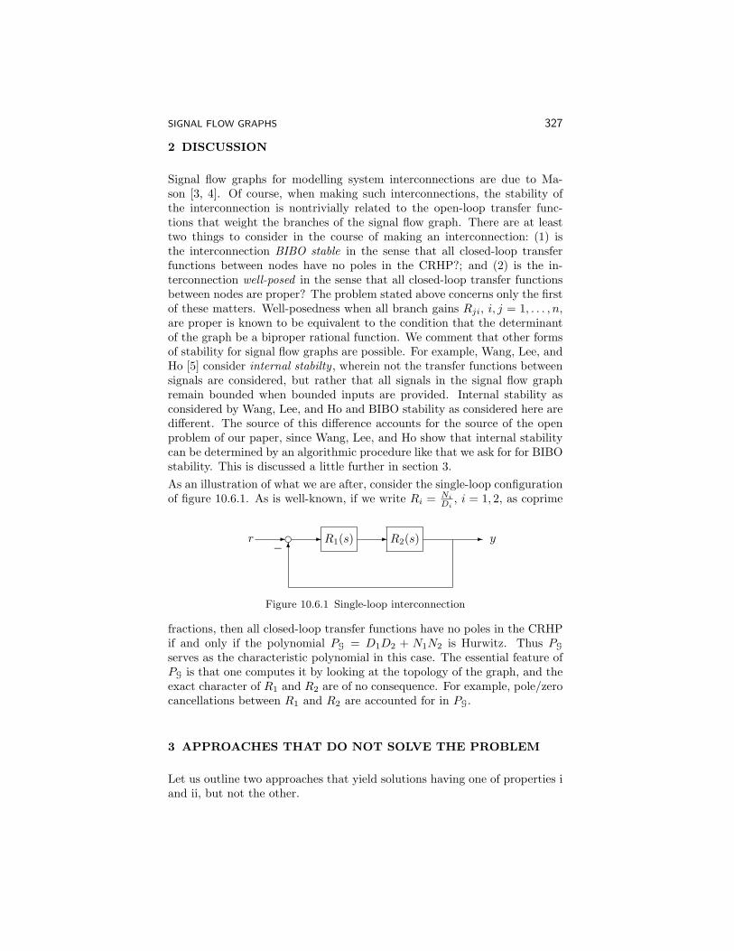
SIGNAL FLOW GRAPHS 327
2 DISCUSSION
Signal flow graphs for modelling system interconnections are due to Ma-son [3, 4]. Of course, when making such interconnections, the stability ofthe interconnection is nontrivially related to the open-loop transfer func-tions that weight the branches of the signal flow graph. There are at leasttwo things to consider in the course of making an interconnection: (1) isthe interconnection BIBO stable in the sense that all closed-loop transferfunctions between nodes have no poles in the CRHP?; and (2) is the in-terconnection well-posed in the sense that all closed-loop transfer functionsbetween nodes are proper? The problem stated above concerns only the firstof these matters. Well-posedness when all branch gains Rji, i, j = 1, . . . , n,are proper is known to be equivalent to the condition that the determinantof the graph be a biproper rational function. We comment that other formsof stability for signal flow graphs are possible. For example, Wang, Lee, andHo [5] consider internal stabilty , wherein not the transfer functions betweensignals are considered, but rather that all signals in the signal flow graphremain bounded when bounded inputs are provided. Internal stability asconsidered by Wang, Lee, and Ho and BIBO stability as considered here aredifferent. The source of this difference accounts for the source of the openproblem of our paper, since Wang, Lee, and Ho show that internal stabilitycan be determined by an algorithmic procedure like that we ask for for BIBOstability. This is discussed a little further in section 3.As an illustration of what we are after, consider the single-loop configurationof figure 10.6.1. As is well-known, if we write Ri = Ni
Di, i = 1, 2, as coprime
-r d - R1(s) - R2(s) - y6−
Figure 10.6.1 Single-loop interconnection
fractions, then all closed-loop transfer functions have no poles in the CRHPif and only if the polynomial PG = D1D2 + N1N2 is Hurwitz. Thus PG
serves as the characteristic polynomial in this case. The essential feature ofPG is that one computes it by looking at the topology of the graph, and theexact character of R1 and R2 are of no consequence. For example, pole/zerocancellations between R1 and R2 are accounted for in PG.
3 APPROACHES THAT DO NOT SOLVE THE PROBLEM
Let us outline two approaches that yield solutions having one of properties iand ii, but not the other.
328 PROBLEM 10.6
The problems of internal stability and well-posedness for signal flow graphscan be handled effectively using the polynomial matrix approach, e.g., [1].Such an approach will involve the determination of a coprime matrix frac-tional representation of a matrix of rational functions. This will certainlysolve the problem of determining internal stability for any given example.That is, it is possible using matrix polynomial methods to provide an algo-rithmic construction of a polynomial satisfying property ii above. However,the algorithmic procedure will involve computing GCDs of various of thepolynomials Nji and Dji, i, j = 1, . . . , n. Thus the conditions developed inthis manner have to do not only with the topology of the signal flow graph,but also the specific choices for the branch gains, thus violating condition iabove. The problem we pose demands a simpler, more direct answer to thequestion of determining when an interconnection is BIBO stable.Wang, Lee, and He [5] provide a polynomial for a signal flow graph using thedeterminant of the graph which we denote by ∆G (see [3, 4]). Specifically,they define a polynomial
P =∏
(i,j)∈1,...,n2Dji∆G. (1)
Thus one multiplies the determinant by all denominators, arriving at a poly-nomial in the process. This polynomial has the property i above. However,while it is true that if this polynomial is Hurwitz then the system is BIBOstable, the converse is generally false. Thus property ii is not satisfied by P .What is shown in [5] is that all signals in the graph are bounded for boundedinputs if and only if P is Hurwitz. This is different from what we are askinghere, i.e., that all closed-loop transfer functions have no CRHP poles. It istrue that the polynomial P in (1) gives the desired characteristic polyno-mial for the interconnection of Figure 10.6.1. It is also true that if the signalflow graph has no loops (in this case ∆G = 1) then the polynomial P of (1)satisfies condition ii. We comment that the condition of Wang, Lee, andHo is the same condition one would obtain by converting (in a specific way)the signal flow graph to a polynomial matrix system, and then ascertainingwhen the resulting polynomial matrix system is internally stable.The problem stated is very basic, one for which an inquisitive undergraduatewould demand a solution. It was with some surprise that the author wasunable to find its solution in the literature, and hopefully one of the readersof this article will be able to provide a solution, or point out an existing one.
BIBLIOGRAPHY
[1] F. M. Callier and C. A. Desoer, Multivariable Feedback Systems,Springer-Verlag, New York-Heidelberg-Berlin, 1982.
[2] A. D. Lewis, “On the stability of interconnections of SISO, time-invariant, finite-dimensional, linear systems,” preprint, July 2001.
SIGNAL FLOW GRAPHS 329
[3] S. J. Mason, “Feedback theory: Some properties of signal flow graphs,”Proc. IRE, 41:1144–1156, 1953.
[4] S. J. Mason, “Feedback theory: Further properties of signal flow graphs,”Proc. IRE, 44:920–926, 1956.
[5] Q.-G. Wang, T.-H. Lee, and J.-B. He, “Internal stability of intercon-nected systems,” IEEE Trans. Automat. Control, 44(3):593–596, 1999.
Problem 10.7
Open problems in randomized µ analysis
Onur TokerCollege of Computer Sciences and EngineeringKFUPM, P.O. Box 14Dhahran 31261Saudi [email protected]
1 INTRODUCTION
In this chapter, we review the current status of the problem reported in [5],and discuss some open problems related to randomized µ analysis. Basically,what remains still unknown after Treil’s result [6] are the growth rate of theµ/µ ratio, and how likely it is to observe a high conservatism. In the contextof randomized µ analysis, we discuss two open problems (i) Existence ofpolynomial time Las Vegas type randomized algorithms for robust stabilityagainst structured LTI uncertainties, and (ii) The minimum sample size toguarantee that µ/µ conservatism will be bounded by g, with a confidencelevel of 1− ε.
2 DESCRIPTION AND HISTORY OF THE PROBLEM
The structured singular value [1] is a quite general framework for analy-sis/design against component level LTI uncertainties. Although for smallnumber of uncertain blocks, the problem is of reasonable difficulty, all ini-tial studies implied that the same is not likely to be true for the generalcase. Under these observations, convex upper bound tests became popularalternatives for the structured singular value. Later, it has been proved thatthese upper bound tests are indeed nonconservative robustness measures fordifferent classes of component level uncertainties, and the structured sin-gular value analysis problem is NP-hard. See the paper [5] and referencestherein for further details on the history of the problem.
OPEN PROBLEMS IN RANDOMIZED µ ANALYSIS 331
What remains still open after Treil’s result? An important openproblem was the conservativeness of the standard upper bound test for thecomplex µ [5]. Recently, Treil showed that the gap between µ and its upperbound µ can be arbitrarily large [6]. Despite this negative result, computa-tional experiments show that most of the time the gap is very close to onefor matrices of reasonable size. The following are still open problems:
• What is the growth rate of the gap? In other words, what is the growthrate of
supµ(M) 6=0
µ(M)µ(M)
as a function of n = dim(M). It is suspected that the growth rate isO(log(n)) [6].
• How likely it is to observe low conservatism? In other words, what isthe relative volume of the set
M : (1 + ε)µ(M) ≥ µ(M) ≥ µ(M)in the set of all n × n matrices with all entries having absolute valueat most 1.
Randomized algorithms and some open problems Randomized al-gorithms are known to be quite powerful tools for dealing with difficultproblems. A recent paper of Vidyasagar and Blondel [8] has both a nicesummary of earlier results in this area, and provides a strong justificationfor the importance of randomized algorithms for tackling difficult controlrelated problems. Randomized structured singular value analysis is studiedin detail in the recent paper [3], which also has many references to relatedwork in this area.
Las Vegas type algorithm for µ analysis
There are two possible ways of utilizing the results of randomized algorithms,in particular the randomized µ analysis. Let us assume that several randomuncertainty matrices with norm bounded by 1, ∆k’s, k = 1, · · · , S, are gen-erated according to some probability distribution, and µ(M) is set to
µ(M) = max1≤k≤S
ρ(M∆k).
The first interpretation is the following: with a high probability, the inequal-ity ρ(M∆) ≤ µ(M) is satisfied for all ∆’s except for a set of small relativevolume [7]. The second interpretation is to consider the whole process ofgenerating random ∆ samples and checking the condition ρ(M∆) < 1, asa Monte Carlo type algorithm for the complement of robust stability [2].Indeed, after generating several ∆ samples, if µ(M) ≥ 1, then the (M,∆)system is not robustly stable, otherwise one can either say the test is in-conclusive or conclude that the (M,∆) system is robustly stable (which
332 PROBLEM 10.7
sometimes can be the wrong conclusion). This unpleasant phenomena is astandard characteristic of Monte Carlo algorithms. What is not known iswhether there is also a polynomial time Monte Carlo type randomized algo-rithm for the robust stability condition itself. Combining these two MonteCarlo algorithms will result an algorithm that never gives a false answer, andthe probability of getting inconclusive answers goes to zero as we generatemore and more random samples.
Problem 1 (Las Vegas type algorithm for µ analysis): Is there apolynomial time Las Vegas type randomized algorithm for testing robuststability against structured LTI uncertainties?
Why this problem is important?
An algorithm like this can be used to check whether the (M,∆) systemis robustly stable or not by generating random ∆ matrices: There is nopossibility of getting false answers, and probability of getting inconclusiveanswers goes to zero as the sample size goes to infinity. However, the rateof convergence of the probability of getting inconclusive answers to zero, isalso an important factor for the algorithm to be practical.
Relationship between the conservatism of µ/µ, sample size, and confidencelevels
Conservativeness of the randomized lower bound µ is also an open problem.More precisely, we have very little knowledge about the relationship betweenthe conservatism ratio µ/µ, the sample size S, and the conservatism boundg. For simplicity, let n denotes the dimension of the matrix M for the restof this section. The following is a major open problem:
Problem 2: Find the best lower found, S(n, g, ε), such that generatingS ≥ S(n, g, ε) random samples is enough to claim that, for all M ,
µ(M) ≥ max1≤k≤S(n,g,ε)
ρ(M∆k) ≥ g−1µ(M), with confidence level ≥ 1− ε.
In other words, the probability inequality
Prob
∆1, · · · ,∆S(n,g,ε) : µ(M) ≥ max1≤k≤S(n,g,ε)
ρ(M∆k) ≥ g−1µ(M)≥
≥ 1− ε,
is satisfied for all M matrices.
Why this is an important problem?
In a robust stability analysis, one can set a confidence level very close one, say1 − 10−6, generate many random ∆ samples, and compute the randomized
OPEN PROBLEMS IN RANDOMIZED µ ANALYSIS 333
lower bound µ. Ideally, a control engineer would like know how conservativeis the obtained µ compared to the actual µ, in order to have a better feelingof the system at hand.There is very little known about this problem, and some partial results arereported in [4]. The following are simple corollaries:Result 1 (Polynomial number of samples): For any positive universalconstants C,α ∈ Z, generating Sn = Cnα random samples is not enough toclaim that, for all M ,
µ(M) ≥ max1≤k≤Sn
ρ(M∆k) ≥ 0.99µ(M), with confidence level ≥ 1− 10−6.
Result 2 (Exponential number of samples): There is a universal con-stant C such that, generating Sn = Cen
2.01random samples is enough to
claim that, for all M ,
µ(M) ≥ max1≤k≤Sn
ρ(M∆k) ≥ 0.99µ(M), with confidence level ≥ 1− 10−6.
Alternatively, one can fix a confidence level, say 1 − 10−6, and study therelationship between the sample size S, and the best conservatism bound,g(S), that can be guaranteed with this confidence level. Again not much isknown about how fast/slow the best conservatism bound g(S) converges to1 as the sample size S goes to infinity.
BIBLIOGRAPHY
[1] A. Packard and J. C. Doyle, “The complex structured singular value,”Automatica, 29, pp. 71–109, 1993.
[2] Papadimitriou, C. H., Computational Complexity, Addison-Wesley, 1994.
[3] G. C. Calafiore, F. Dabbene, and R. Tempo,“Randomized algorithms forprobabilistic robustness with real and complex structured uncertainty,”IEEE Transactions on Automatic Control, vol. 45, pp. 2218–2235, 2000.
[4] O. Toker, “Conservatism of Randomized Structured Singular Value,”accepted for publication in IEEE Transactions on Automatic Control.
[5] O. Toker, and B. Jager, “Conservatism of the Standard Upper BoundTest: Is sup(µ/µ) finite? Is it bounded by 2?,” In: Open Problemsin Mathematical Systems and Control Theory, V. Blondel, et al. eds.,chapter 43, pp. 225–228.
[6] S. Treil, “The gap between complex structured singular value µ andits upper bound is infinite,” Forthcoming In: IEEE Transactions onAutomatic Control.

334 PROBLEM 10.7
[7] M. Vidyasagar, A Theory of Learning and Generalization, Springer-Verlag, London, 1997.
[8] M. Vidyasagar and V. Blondel, “Probabilistic solutions to some NP-hardmatrix problems,” Automatica, vol. 37, pp. 1397–1405, 2001.