unsteady simulation of a 1.5 stage turbine using an implicitly...

UNSTEADY SIMULATION OF A 1.5 STAGE TURBINE USING AN IMPLICITLYCOUPLED NONLINEAR HARMONIC BALANCE METHOD

Chad H. Custer ∗

CD-adapcoNorthville, Michigan, 48167

Email: [email protected]

Jonathan M. WeissCD-adapco

Lebanon, New Hampshire, 03766

Venkataramanan SubramanianCD-adapco

Bangalore, Karnataka, India

William S. ClarkCD-adapco

Northville, Michigan, 48167

Kenneth C. HallDuke University

Department of Mechanical Engineeringand Materials Science

Durham, North Carolina, 27708

ABSTRACTThe harmonic balance method implemented within STAR-

CCM+ is a mixed frequency/time domain computational fluid dy-namic technique, which enables the efficient calculation of time-periodic flows. The unsteady solution is stored at a small numberof fixed time levels over one temporal period of the unsteady flowin a single blade passage in each blade row; thus the solutionis periodic by construction. The individual time levels are cou-pled to one another through a spectral operator representing thetime derivative term in the Navier-Stokes equation, and at theboundaries of the computational domain through the applicationof periodic and nonreflecting boundary conditions. The bladerows are connected to one another via a small number of fluiddynamic spinning modes characterized by nodal diameter andfrequency. This periodic solution is driven to the correct solutionusing conventional (steady) CFD acceleration techniques, andthus is computationally efficient. Upon convergence, the timelevel solutions are Fourier transformed to obtain spatially vary-ing Fourier coefficients of the flow variables. We find that a smallnumber of time levels (or, equivalently, Fourier coefficients) areadequate to model even strongly nonlinear flows. Consequently,the method provides an unsteady solution at a computational

∗Address all correspondence to this author.

cost significantly lower than traditional unsteady time marchingmethods.

The implementation of this nonlinear harmonic balancemethod within STAR-CCM+ allows for the simulation of mul-tiple blade rows. This capability is demonstrated and validatedusing a 1.5 stage cold flow axial turbine developed by the Uni-versity of Aachen. Results produced using the harmonic balancemethod are compared to conventional time domain simulationsusing STAR-CCM+, and are also compared to published exper-imental data. It is shown that the harmonic balance method isable to accurately model the unsteady flow structures at a com-putational cost significantly lower than unsteady time domainsimulation.

INTRODUCTIONAccurate and efficient prediction of the unsteady nature of

time-periodic flows is essential to improving the performanceof multi-stage turbomachines. Steady mixing-plane simula-tion methods have been widely used to analyze turbomachineryflows. However, the actual flow through blade rows is inherentlyunsteady. To further improve predictive capabilities, the influ-ence of unsteady flows on loss production caused by wake in-teraction, shock wave interaction, potential flow interaction, and

Proceedings of ASME Turbo Expo 2012 GT2012

June 11-15, 2012, Copenhagen, Denmark

GT2012-69690

1 Copyright © 2012 by ASME

secondary flow interaction must be better understood. Both ex-perimental [1–3] and numerical [4–6] studies have emphasizedthe importance of modeling such unsteady effects.

Harmonic BalanceUnsteady flows in turbomachinery have traditionally been

modeled either by nonlinear time domain methods [7] or by fre-quency domain or time-linearized theories [8, 9]. In the timedomain approach, the governing equations are discretized on acomputational mesh using conventional CFD methods, and thenonlinear unsteady flow is evolved in time by time-accuratelyadvancing the solution from one time instant to the next. Whilenonlinear disturbances are captured by this approach, stabilityand accuracy considerations require the use of small time steps.As a result, the computational cost associated with time domainmethods is often quite large, especially for multi-row turboma-chines.

In the so-called “time-linearized” (frequency-domain) ap-proach, the time-mean or steady flow is first computed by solv-ing the steady flow equations within the computational domain.Then, the unsteady flow equations are linearized about this mean,assuming that the unsteadiness is small and harmonic in time [8].A recent survey of frequency domain approaches has been re-ported by He [10]. Other transformation and scaling methodsthat attempt to reduce the size of the computational domain mod-eled have also been reported in the literature [11].

The harmonic balance method developed by Hall, et al. [12],is a mixed time domain and frequency domain approach. Thismethod is a computationally efficient way of solving nonlin-ear, unsteady, periodic flows containing arbitrarily large distur-bances, in multi-stage machines with unequal blade counts. Inthis approach, each blade row is modeled using a computationalgrid that spans only one blade passage, regardless of the inter-blade phase angle. This is made possible by using phase-laggedperiodic boundary conditions. Within each blade row, the flowsolution is stored at several time-levels within one temporal pe-riod. Thus, the solution is periodic by construction. These timelevel solutions are coupled to each other at the periodic bound-aries through the application of complex periodicity conditions;at the far field, through the application of nonreflecting boundaryconditions; at the inter-row interfaces; and in the flow field itself,through the use of a pseudo-spectral time derivative operator.

Several variants and extensions of the harmonic balancemethod have been developed by Gopinath and Jameson [13], Mc-Mullen, et al. [14], Nadarajah, et al. [15], and others [16]. Re-cently, Dufour, et al. [17] have reported comparisons of the time-linearized methods and the harmonic balance method. Whileinitial implementation of the harmonic balance approach usedexplicit time marching solvers like Lax Wendroff or Runge-Kutta schemes, recent implementations of the harmonic balancemethod have made use of implicit solvers to provide better nu-

merical stability and faster convergence rates [18,19]. This paperuses the implementation of the implicitly coupled harmonic bal-ance approach described by Weiss, et al. [20].

Aachen TurbineThe Aachen turbine is a 1.5 stage cold flow turbine housed

at the Institute of Jet Propulsion and Turbomachinery at RWTHAachen, Germany. The machine has a constant hub radius of145 mm and a constant shroud radius of 300 mm. The upstreamand downstream vanes are geometrically identical and are con-structed from an untwisted Traupel profile stacked at the trailingedge. The second vane row can be clocked relative to the firstvane row. The rotor consists of an untwisted, modified VKI pro-file stacked at the center of gravity. There is a 15 mm axial gapbetween each of the blades.

Steady and unsteady data has been obtained at various loca-tions within the machine. Using this data, flow structures such asblade tip vortices have been observed and characterized [21,22].The influence of rotor tip clearance on the unsteady flow struc-tures has been studied [23]. Additionally, blade row interactionhas been studied with a focus on how vane clocking affects un-steady flow [24].

Simulation methods have also been applied to the geometry.For instance, the influence of blade fillets on aerodynamic per-formance has been investigated [25]. Additionally, CFD solvershave been validated against the Aachen test data [26,27].

Steady and unsteady data is available for two test configura-tions. The first configuration corresponds to a mass flow rate ofabout 7 kg/s with vane row 2 clocked 3 degrees in the directionof rotation. The second configuration is for a mass flow rate ofabout 8 kg/s and a vane 2 clocking of 2 degrees opposite the di-rection of rotation. The 8 kg/s mass flow rate is considered here.The rotation rate for this configuration is 3500 rpm, which re-sults in a Mach number of about 0.49 at the axial plane betweenthe upstream vane and the rotor. Numerous experimental trialswere run at these conditions to obtain data at each of the axialplane test sections. The mass flow rate observed during thesetrials ranged from 7.75 kg/s to 8.02 kg/s.

COMPUTATIONAL METHODThe unsteady flow field in a turbomachine blade passage is

governed by the Navier-Stokes equations, shown here in integralform for a rigid, arbitrary control volumeV with differential sur-face aread~A in a relative frame of reference rotating steadily withangular velocityΩ:

∫

V

∂W∂ t

dV +

∮

[

~F −~G]

·d~A =

∫

VSdV (1)


whereW = [ρ ,ρu,ρE]T is the solution vector of conservationvariables,~F and~G are the standard inviscid and viscous fluxvectors, andS= [0,ρ Ω⊗u,0]T is the source term due to rota-tion. Density, absolute velocity, total enthalpy, and pressure arerepresented byρ , u, E, andp, respectively.

Flow Field KinematicsThe frequencies and wavelengths of disturbances within the

rows of a multistage machine are determined by the blade countsin the individual blade rows and the rotation rate of the rotor.Consider, for example, a three-row section of a turbine com-prised of a vane/rotor/vane with respective blade countsB1, B2,andB3. Disturbances in the three blade rows will have circum-ferential waves numbers (nodal diameters) equal to

N = m1B1 +n2B2 +m3B3 (2)

wherem1, m2, andm3 can take on all integer values. The fre-quency in the stationary frame of reference is given by

ω = n2B2Ω (3)

In the rotor frame of reference, the frequencies are given by

ω = −(n1B1 +n3B3)Ω (4)

As a practical matter and as will be shown, we need to retainonly a handful of the infinite set of potential nodal diameters andfrequencies in the harmonic balance analysis to obtain accurateunsteady flow solutions. Regardless, the selection of the set ofintegersn1, n2, andn3 determines the unique frequencies in theharmonic balance analysis.

Harmonic Balance EquationsSince the solutionW is periodic in time, it can be represented

by the Fourier series:

W(~x,t) =M

∑m=−M

Wm(~x)eiωmt (5)

whereω is the fundamental frequency of the disturbance,M isthe number of harmonics retained in the solution, andWm arethe Fourier coefficients. The coefficientsWm can be uniquelydetermined from the discrete Fourier transform:

Wm(~x) =1N

N−1

∑n=0

W∗n(~x,tn)e−iωmtn (6)

whereW∗ are a set ofN = 2M+1 solutions at discrete time levelstn = nT/N distributed throughout one period of unsteadiness,T.

The governing equations, Eqn. (1), are then applied to all theW∗ simultaneously, where the time derivative term in Eqn. (1) isreplaced by differentiating Eqn. (5) with respect to time. Thesolutions at each discrete time level are obtained by solving theresultant steady, harmonic balance equations

∫

VDW∗dV +

∮

[

~F∗−~G

∗]

·d~A =

∫

VS∗dV (7)

where D is theN×N pseudo-spectral matrix operator, and theflux and source vectors~F

∗, ~G

∗, andS∗ are evaluated using the

corresponding time level solution.

Solution ProcedureThe harmonic balance equations of Eqn. (7) are discretized

by means of a cell-centered, polyhedral-based, finite-volumescheme having second order spatial accuracy. The convectivefluxes are evaluated by a standard upwind, flux-difference split-ting and the diffusive fluxes by a second-order central difference.A pseudo-time derivative is introduced into the discretized equa-tions to facilitate solution of the steady, harmonic balance equa-tions by means of a time marching procedure. An Euler implicitdiscretization in pseudo-time is applied to yield a coupled, linearsystem containing equations from all time levels linked at everypoint in the domain by the pseudo-spectral operator D. Approx-imate factorization is employed to effectively decouple the timelevels, and an algebraic multigrid (AMG) method is used to solvethe linear system associated with each time level. Further detailsof the solution methodology can be found in reference [20].

Boundary ConditionsPeriodic Boundaries. At each iteration of the harmonic

balance solver, complex periodicity conditions are applied at theperiodic boundaries in the rotational direction to reduce the com-putational domain to a single passage in each row. The process isas follows. First, the solution (which is stored at a discrete set oftime levels) is Fourier transformed in time to obtain the temporalFourier coefficients of the flow along the boundaries. Then, foreach Fourier coefficient, we apply the complex boundary condi-tion

Wm(r,θ ,z) = Wm(r,θ +G,z)e−iNmG (8)

whereWm(r,θ ,z) andWm(r,θ +G,z) are themth Fourier coeffi-cient of the solution on the lower and upper periodic boundaries,respectively. Finally, the solution is inverse Fourier transformedto obtain the solution at the discrete time levels over one period.


Far Field Boundaries. Af ter each iteration of the flowsolver, non-reflecting, far field boundary conditions are appliedat the inflow and outflow boundaries of the domain to preventspurious unsteady numerical disturbances from reflecting backinto the computational domain. This permits the use of truncatedcomputational domains, with boundaries positioned near to theleading and trailing edges of the outermost blade rows. In the farfield, the solution may be thought of as comprised of upstreamand downstream moving waves. The frequency and nodal diam-eter of these waves are described in the “Flow Field Kinematics”section. At each radial station along the far field, we apply two-dimensional nonreflecting boundary conditions.

The procedure begins by computing the temporal Fourier co-efficients at all points along the boundary. Next, thesetemporalFourier coefficients are Fourier transformed in thecircumferen-tial direction. The result of this double Fourier transform is fivecoefficients at each radial station for each kinematic mode, onefor each primitive variable (pressure; temperature; and axial, ra-dial, and circumferential velocities.)

Next, except for the zero nodal diameter steady mode, a five-by-five eigenanalysis is then performed to identify the magni-tude of incoming and outgoing wave components. The outgoingwaves are left unmodified, and the incoming waves are zeroedout. For the zero nodal diameter steady modes, traditional steadyinflow or outflow boundary conditions are applied. Total pres-sure, total temperature, and flow angle of the mean flow are spec-ified at the inflow boundary, and the static pressure of the meanflow is specified at the outflow boundary.

Finally, having modified the far field spinning modes, themode coefficients are inverse Fourier transformed in space andtime to obtain the time level solutions along the far field bound-ary.

Inter-Row Boundaries. The inter-row boundary condi-tions, which connect the solutions in neighboring blade rows, areapplied after each iteration of the flow solver. This procedure fol-lows closely that described above for far field boundaries. Thesolutions along the interface boundaries between two blade rowsare Fourier transformed in space and time at each radial station toobtain the coefficients of the spinning modes. If a given spinningmode exists in both blade rows, the mode coefficients on eitherside of the interface are set equal to one another (the average ofthe coefficients). If a given spinning mode exists on only oneside, nonreflecting boundary conditions are applied as describedin the previous section. Finally, the modified Fourier coefficientsare inverse transformed in time and space to yield updated solu-tions on the inter-row boundaries.

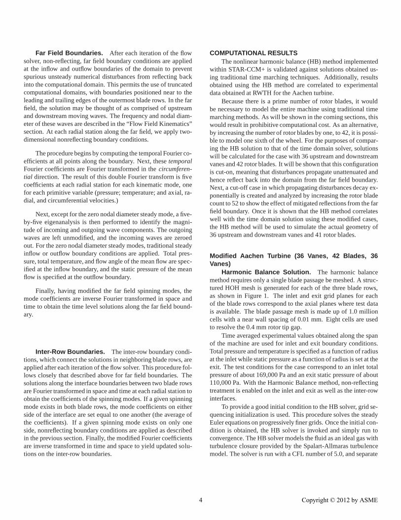
COMPUTATIONAL RESULTSThe nonlinear harmonic balance (HB) method implemented

within STAR-CCM+ is validated against solutions obtained us-ing traditional time marching techniques. Additionally, resultsobtained using the HB method are correlated to experimentaldata obtained at RWTH for the Aachen turbine.

Because there is a prime number of rotor blades, it wouldbe necessary to model the entire machine using traditional timemarching methods. As will be shown in the coming sections, thiswould result in prohibitive computational cost. As an alternative,by increasing the number of rotor blades by one, to 42, it is possi-ble to model one sixth of the wheel. For the purposes of compar-ing the HB solution to that of the time domain solver, solutionswill be calculated for the case with 36 upstream and downstreamvanes and 42 rotor blades. It will be shown that this configurationis cut-on, meaning that disturbances propagate unattenuated andhence reflect back into the domain from the far field boundary.Next, a cut-off case in which propagating disturbances decay ex-ponentially is created and analyzed by increasing the rotor bladecount to 52 to show the effect of mitigated reflections from the farfield boundary. Once it is shown that the HB method correlateswell with the time domain solution using these modified cases,the HB method will be used to simulate the actual geometry of36 upstream and downstream vanes and 41 rotor blades.

Modified Aachen Turbine (36 Vanes, 42 Blades, 36Vanes)

Harmonic Balance Solution. The harmonic balancemethod requires only a single blade passage be meshed. A struc-tured HOH mesh is generated for each of the three blade rows,as shown in Figure 1. The inlet and exit grid planes for eachof the blade rows correspond to the axial planes where test datais available. The blade passage mesh is made up of 1.0 millioncells with a near wall spacing of 0.01 mm. Eight cells are usedto resolve the 0.4 mm rotor tip gap.

Time averaged experimental values obtained along the spanof the machine are used for inlet and exit boundary conditions.Total pressure and temperature is specified as a function of radiusat the inlet while static pressure as a function of radius is set at theexit. The test conditions for the case correspond to an inlet totalpressure of about 169,000 Pa and an exit static pressure of about110,000 Pa. With the Harmonic Balance method, non-reflectingtreatment is enabled on the inlet and exit as well as the inter-rowinterfaces.

To provide a good initial condition to the HB solver, grid se-quencing initialization is used. This procedure solves the steadyEuler equations on progressively finer grids. Once the initial con-dition is obtained, the HB solver is invoked and simply run toconvergence. The HB solver models the fluid as an ideal gas withturbulence closure provided by the Spalart-Allmaras turbulencemodel. The solver is run with a CFL number of 5.0, and separate


FIGURE 1. COMPUTATIONAL MESH FOR THE HARMONICBALANCE SIMULATION OF THE 36-42-36 GEOMETRY.

1e-06

1e-05

0.0001

0.001

0.01

0.1

1

0 1000 2000 3000 4000 5000 6000 7000

Res

idua

ls

Iteration

ContinuityX-momentumY-momentumZ-momentumEnergySA

FIGURE 2. HARMONIC BALANCE SOLUTION RESIDUALSFOR A THREE MODE TRIAL.

trials are conducted retaining one, three, and five modes. Be-cause the discrete time-level solutions can be readily convertedto the frequency domain, time mean and higher modal contentof monitored variables can be monitored directly. The residualplot shown in Figure 2 corresponds to a trial run in single preci-sion with three modes retained in each of the blade rows. Thisshows that the solver has converged to a periodic, unsteady solu-tion within 5000 iterations.

Time Domain Solution. The mesh used for the time do-main trials is created by duplicating the blade passage mesh togenerate one sixth of the wheel. Additionally, as shown in Fig-ure 3, the vane 2 exit is extruded in the axial direction to mitigatethe possibility of numerical reflections from the far field bound-

FIGURE 3. COMPUTATIONAL MESH FOR THE TIME DOMAINSIMULATION OF THE 36-42-36 GEOMETRY. POINT PROBE IN-DICATED BY THE GREEN DOT DOWNSTREAM OF THE ROTORTRAILING EDGE.

ary.As with the harmonic balance solution procedure, first an

initial condition is obtained using grid sequencing initialization.Once the initial condition is obtained, the unsteady Reynolds-averaged Navier-Stokes solver is initiated. The time domainsolver is based on a dual time-stepping scheme, which integratesthe governing equations in time by sub-iterating at each timestep. A time step corresponding to 101 steps per vane passingis used with 20 sub-iterations per time step.

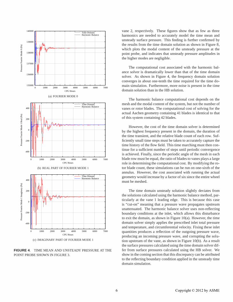
Convergence of the time domain solver is judged by mon-itoring the unsteady pressure at a mid-span point between therotor trailing edge and the downstream vane leading edge, asshown in Figure 3. The time history of pressure at this pointis then subjected to a windowed discrete Fourier transform algo-rithm. This algorithm first resamples the data at equally spacedpoints in time within one rotor passing using a simple linear in-terpolation. This interpolated data is then pre-multiplied by thediscrete Fourier transform matrix using a moving window tech-nique. The modal content of the pressure at the point probe isshown as a function of CPU-time for both the time domain andharmonic balance methods in Figure 4. This figure shows that af-ter about 7000 CPU-hours, the time domain solver has convergedto a reasonable level. This corresponds to 48 rotor periods.

Once periodic convergence is achieved, modal content ofsurface pressure is obtained. Mid-span vane and blade unsteadypressure data is extracted and transformed into the frequency do-main. The resulting modal pressure content is then compared tosolutions obtained using the harmonic balance solver.

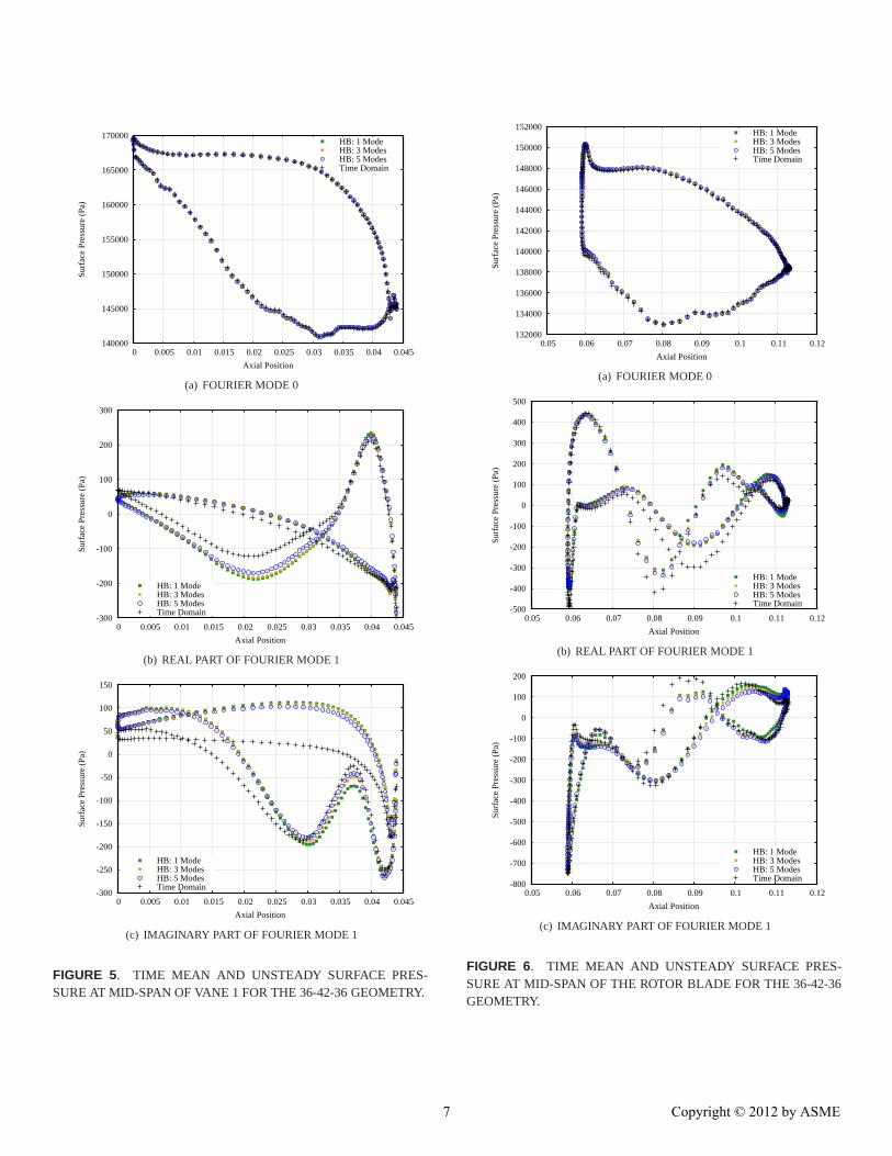
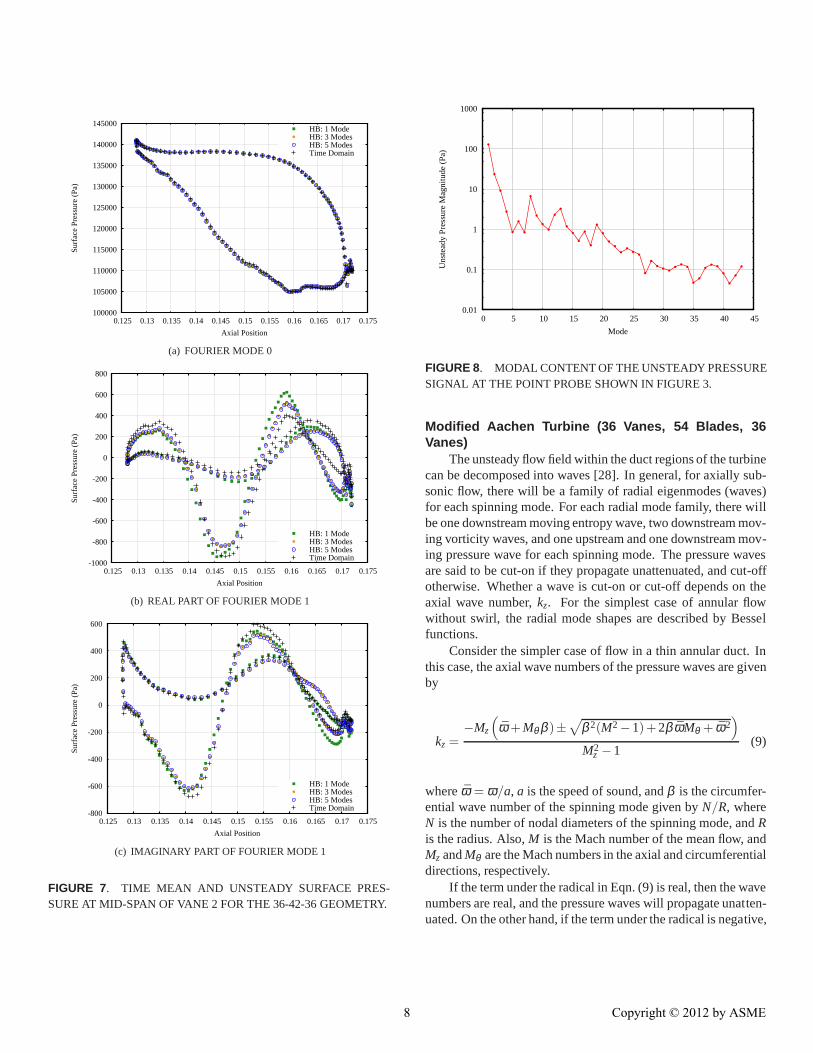
Results. Figures 5, 6, and 7 display the zeroth and firstmode of unsteady pressure at mid-span of vane 1, the rotor, and


135000

136000

137000

138000

139000

140000

0 1000 2000 3000 4000 5000 6000 7000

Pre

ssur

e F

ourie

r M

ode

0 (P

a)

CPU Hours

Time DomainHarmonic Balance

(a) FOURIER MODE 0

-400

-200

0

200

400

0 1000 2000 3000 4000 5000 6000 7000

Pre

ssur

e F

ourie

r M

ode

1 R

eal (

Pa)

CPU Hours


(b) REAL PART OF FOURIER MODE 1

-400

-200

0

200

400

0 1000 2000 3000 4000 5000 6000 7000

Pre

ssur

e F

ourie

r M

ode

1 Im

agin

ary

(Pa)

CPU Hours


(c) IMAGINARY PART OF FOURIER MODE 1

FIGURE 4. TIME MEAN AND UNSTEADY PRESSURE AT THEPOINT PROBE SHOWN IN FIGURE 3.

vane 2, respectively. These figures show that as few as threeharmonics are needed to accurately model the time mean andunsteady surface pressure. This finding is further confirmed bythe results from the time domain solution as shown in Figure 8,which plots the modal content of the unsteady pressure at thepoint probe, and indicates that unsteady pressure amplitudes inthe higher modes are negligible.

The computational cost associated with the harmonic bal-ance solver is dramatically lower than that of the time domainsolver. As shown in Figure 4, the frequency domain solutionconverges in about one-tenth the time required for the time do-main simulation. Furthermore, more noise is present in the timedomain solution than in the HB solution.

The harmonic balance computational cost depends on themesh and the modal content of the system, but not the number ofvanes or rotor blades. The computational cost of solving for theactual Aachen geometry containing 41 blades is identical to thatof this system containing 42 blades.

However, the cost of the time domain solver is determinedby the highest frequency present in the domain, the duration ofthe time transient, and the relative blade count of each row. Suf-ficiently small time steps must be taken to accurately capture thetime history of the flow field. This time marching must then con-tinue for a sufficient number of steps until periodic convergenceis achieved. Finally, since the periodic angle of the mesh in eachblade row must be equal, the ratio of blades to vanes plays a largerole in determining the computational cost. By modifying the ro-tor blade count, these simulations can be run on one-sixth of theannulus. However, the cost associated with running the actualgeometry would increase by a factor of six since the entire wheelmust be meshed.

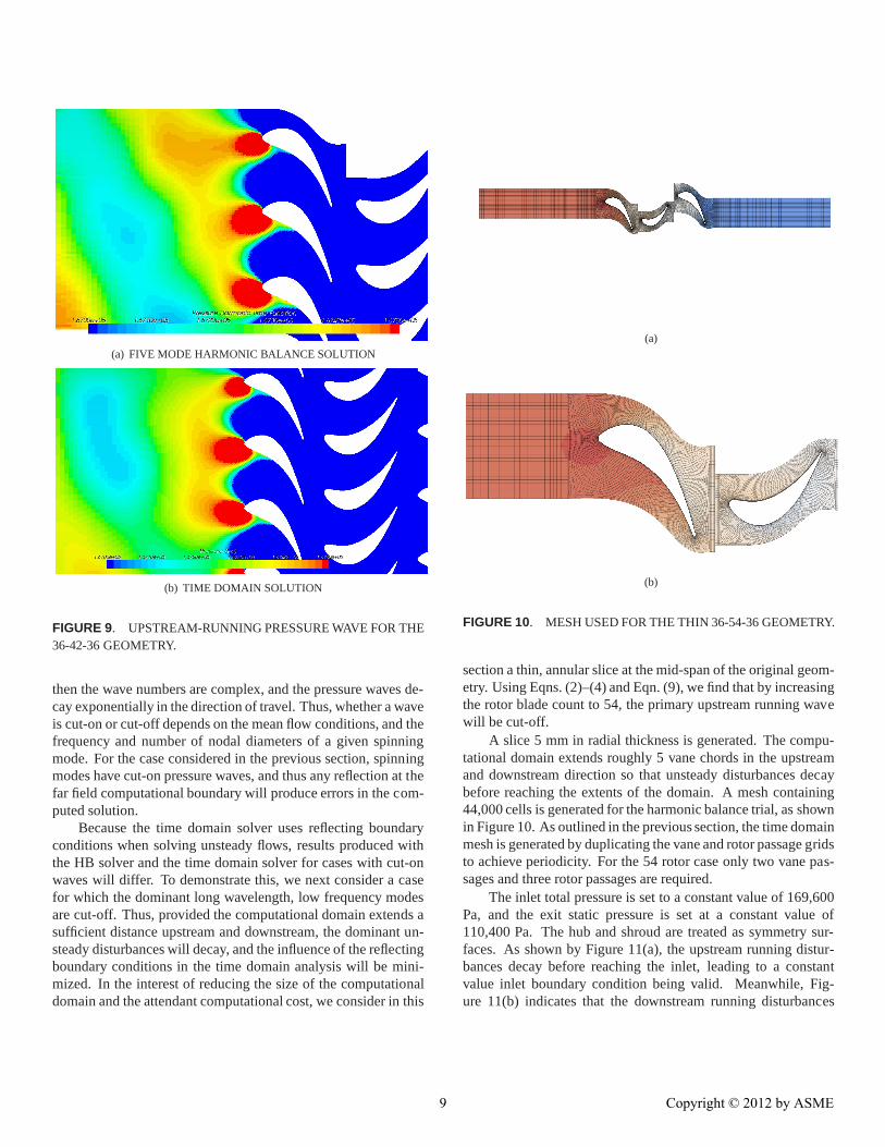
The time domain unsteady solution slightly deviates fromthe solutions calculated using the harmonic balance method, par-ticularly at the vane 1 leading edge. This is because this caseis “cut-on” meaning that a pressure wave propagates upstreamunattenuated. The harmonic balance solver uses non-reflectingboundary conditions at the inlet, which allows this disturbanceto exit the domain, as shown in Figure 10(a). However, the timedomain solver simply applies the prescribed inlet total pressureand temperature, and circumferential velocity. Fixing these inletquantities produces a reflection of the outgoing pressure wave,producing an incoming pressure wave, and corrupting the solu-tion upstream of the vane, as shown in Figure 10(b). As a resultthe surface pressures calculated using the time domain solver dif-fer from surface pressures calculated using the HB solver. Weshow in the coming section that this discrepancy can be attributedto the reflecting boundary condition applied in the unsteady timedomain simulation.


140000

145000

150000

155000

160000

165000

170000

0 0.005 0.01 0.015 0.02 0.025 0.03 0.035 0.04 0.045

Sur

face

Pre

ssur

e (P

a)

Axial Position

HB: 1 ModeHB: 3 ModesHB: 5 ModesTime Domain

(a) FOURIER MODE 0

-300

-200

-100

0

100

200

300

0 0.005 0.01 0.015 0.02 0.025 0.03 0.035 0.04 0.045

Sur

face

Pre

ssur

e (P

a)

Axial Position



-300

-250

-200

-150

-100

-50

0

50

100

150

0 0.005 0.01 0.015 0.02 0.025 0.03 0.035 0.04 0.045

Sur

face

Pre

ssur

e (P

a)

Axial Position



FIGURE 5. TIME MEAN AND UNSTEADY SURFACE PRES-SURE AT MID-SPAN OF VANE 1 FOR THE 36-42-36 GEOMETRY.

132000

134000

136000

138000

140000

142000

144000

146000

148000

150000

152000

0.05 0.06 0.07 0.08 0.09 0.1 0.11 0.12

Sur

face

Pre

ssur

e (P

a)

Axial Position


(a) FOURIER MODE 0

-500

-400

-300

-200

-100

0

100

200

300

400

500

0.05 0.06 0.07 0.08 0.09 0.1 0.11 0.12

Sur

face

Pre

ssur

e (P

a)

Axial Position



-800

-700

-600

-500

-400

-300

-200

-100

0

100

200

0.05 0.06 0.07 0.08 0.09 0.1 0.11 0.12

Sur

face

Pre

ssur

e (P

a)

Axial Position



FIGURE 6. TIME MEAN AND UNSTEADY SURFACE PRES-SURE AT MID-SPAN OF THE ROTOR BLADE FOR THE 36-42-36GEOMETRY.


100000

105000

110000

115000

120000

125000

130000

135000

140000

145000

0.125 0.13 0.135 0.14 0.145 0.15 0.155 0.16 0.165 0.17 0.175

Sur

face

Pre

ssur

e (P

a)

Axial Position


(a) FOURIER MODE 0

-1000

-800

-600

-400

-200

0

200

400

600

800

0.125 0.13 0.135 0.14 0.145 0.15 0.155 0.16 0.165 0.17 0.175

Sur

face

Pre

ssur

e (P

a)

Axial Position



-800

-600

-400

-200

0

200

400

600

0.125 0.13 0.135 0.14 0.145 0.15 0.155 0.16 0.165 0.17 0.175

Sur

face

Pre

ssur

e (P

a)

Axial Position



FIGURE 7. TIME MEAN AND UNSTEADY SURFACE PRES-SURE AT MID-SPAN OF VANE 2 FOR THE 36-42-36 GEOMETRY.

0.01

0.1

1

10

100

1000

0 5 10 15 20 25 30 35 40 45

Uns

tead

y P

ress

ure

Mag

nitu

de (

Pa)

Mode

FIGURE 8. MODAL CONTENT OF THE UNSTEADY PRESSURESIGNAL AT THE POINT PROBE SHOWN IN FIGURE 3.

Modified Aachen Turbine (36 Vanes, 54 Blades, 36Vanes)

The unsteady flow field within the duct regions of the turbinecan be decomposed into waves [28]. In general, for axially sub-sonic flow, there will be a family of radial eigenmodes (waves)for each spinning mode. For each radial mode family, there willbe one downstream moving entropy wave, two downstream mov-ing vorticity waves, and one upstream and one downstream mov-ing pressure wave for each spinning mode. The pressure wavesare said to be cut-on if they propagate unattenuated, and cut-offotherwise. Whether a wave is cut-on or cut-off depends on theaxial wave number,kz. For the simplest case of annular flowwithout swirl, the radial mode shapes are described by Besselfunctions.

Consider the simpler case of flow in a thin annular duct. Inthis case, the axial wave numbers of the pressure waves are givenby

kz =−Mz

(

ω +Mθ β )±√

β 2(M2−1)+2β ωMθ + ω2)

M2z −1

(9)

whereω = ω/a, a is the speed of sound, andβ is the circumfer-ential wave number of the spinning mode given byN/R, whereN is the number of nodal diameters of the spinning mode, andRis the radius. Also,M is the Mach number of the mean flow, andMz andMθ are the Mach numbers in the axial and circumferentialdirections, respectively.

If the term under the radical in Eqn. (9) is real, then the wavenumbers are real, and the pressure waves will propagate unatten-uated. On the other hand, if the term under the radical is negative,


(a) FIVE MODE HARMONIC BALANCE SOLUTION

(b) TIME DOMAIN SOLUTION

FIGURE 9. UPSTREAM-RUNNING PRESSURE WAVE FOR THE36-42-36 GEOMETRY.

then the wave numbers are complex, and the pressure waves de-cay exponentially in the direction of travel. Thus, whether a waveis cut-on or cut-off depends on the mean flow conditions, and thefrequency and number of nodal diameters of a given spinningmode. For the case considered in the previous section, spinningmodes have cut-on pressure waves, and thus any reflection at thefar field computational boundary will produce errors in the com-puted solution.

Because the time domain solver uses reflecting boundaryconditions when solving unsteady flows, results produced withthe HB solver and the time domain solver for cases with cut-onwaves will differ. To demonstrate this, we next consider a casefor which the dominant long wavelength, low frequency modesare cut-off. Thus, provided the computational domain extends asufficient distance upstream and downstream, the dominant un-steady disturbances will decay, and the influence of the reflectingboundary conditions in the time domain analysis will be mini-mized. In the interest of reducing the size of the computationaldomain and the attendant computational cost, we consider in this

(a)

(b)

FIGURE 10. MESH USED FOR THE THIN 36-54-36 GEOMETRY.

section a thin, annular slice at the mid-span of the original geom-etry. Using Eqns. (2)–(4) and Eqn. (9), we find that by increasingthe rotor blade count to 54, the primary upstream running wavewill be cut-off.

A slice 5 mm in radial thickness is generated. The compu-tational domain extends roughly 5 vane chords in the upstreamand downstream direction so that unsteady disturbances decaybefore reaching the extents of the domain. A mesh containing44,000 cells is generated for the harmonic balance trial, as shownin Figure 10. As outlined in the previous section, the time domainmesh is generated by duplicating the vane and rotor passage gridsto achieve periodicity. For the 54 rotor case only two vane pas-sages and three rotor passages are required.

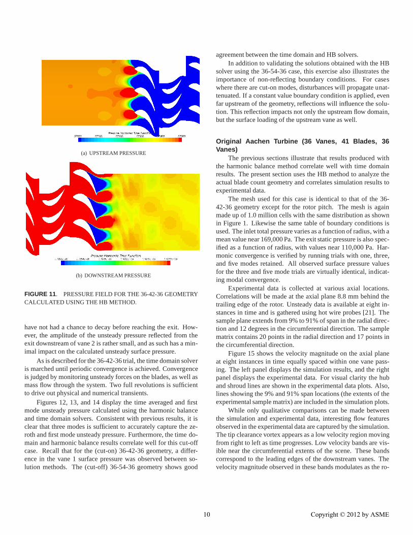
The inlet total pressure is set to a constant value of 169,600Pa, and the exit static pressure is set at a constant value of110,400 Pa. The hub and shroud are treated as symmetry sur-faces. As shown by Figure 11(a), the upstream running distur-bances decay before reaching the inlet, leading to a constantvalue inlet boundary condition being valid. Meanwhile, Fig-ure 11(b) indicates that the downstream running disturbances


(a) UPSTREAM PRESSURE

(b) DOWNSTREAM PRESSURE

FIGURE 11. PRESSURE FIELD FOR THE 36-42-36 GEOMETRYCALCULATED USING THE HB METHOD.

have not had a chance to decay before reaching the exit. How-ever, the amplitude of the unsteady pressure reflected from theexit downstream of vane 2 is rather small, and as such has a min-imal impact on the calculated unsteady surface pressure.

As is described for the 36-42-36 trial, the time domain solveris marched until periodic convergence is achieved. Convergenceis judged by monitoring unsteady forces on the blades, as well asmass flow through the system. Two full revolutions is sufficientto drive out physical and numerical transients.

Figures 12, 13, and 14 display the time averaged and firstmode unsteady pressure calculated using the harmonic balanceand time domain solvers. Consistent with previous results, it isclear that three modes is sufficient to accurately capture the ze-roth and first mode unsteady pressure. Furthermore, the time do-main and harmonic balance results correlate well for this cut-offcase. Recall that for the (cut-on) 36-42-36 geometry, a differ-ence in the vane 1 surface pressure was observed between so-lution methods. The (cut-off) 36-54-36 geometry shows good

agreement between the time domain and HB solvers.In addition to validating the solutions obtained with the HB

solver using the 36-54-36 case, this exercise also illustrates theimportance of non-reflecting boundary conditions. For caseswhere there are cut-on modes, disturbances will propagate unat-tenuated. If a constant value boundary condition is applied, evenfar upstream of the geometry, reflections will influence the solu-tion. This reflection impacts not only the upstream flow domain,but the surface loading of the upstream vane as well.

Original Aachen Turbine (36 Vanes, 41 Blades, 36Vanes)

The previous sections illustrate that results produced withthe harmonic balance method correlate well with time domainresults. The present section uses the HB method to analyze theactual blade count geometry and correlates simulation results toexperimental data.

The mesh used for this case is identical to that of the 36-42-36 geometry except for the rotor pitch. The mesh is againmade up of 1.0 million cells with the same distribution as shownin Figure 1. Likewise the same table of boundary conditions isused. The inlet total pressure varies as a function of radius, with amean value near 169,000 Pa. The exit static pressure is also spec-ified as a function of radius, with values near 110,000 Pa. Har-monic convergence is verified by running trials with one, three,and five modes retained. All observed surface pressure valuesfor the three and five mode trials are virtually identical, indicat-ing modal convergence.

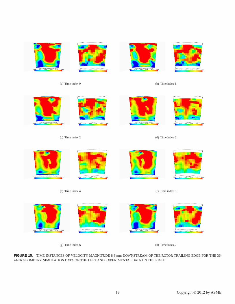
Experimental data is collected at various axial locations.Correlations will be made at the axial plane 8.8 mm behind thetrailing edge of the rotor. Unsteady data is available at eight in-stances in time and is gathered using hot wire probes [21]. Thesample plane extends from 9% to 91% of span in the radial direc-tion and 12 degrees in the circumferential direction. The samplematrix contains 20 points in the radial direction and 17 points inthe circumferential direction.

Figure 15 shows the velocity magnitude on the axial planeat eight instances in time equally spaced within one vane pass-ing. The left panel displays the simulation results, and the rightpanel displays the experimental data. For visual clarity the huband shroud lines are shown in the experimental data plots. Also,lines showing the 9% and 91% span locations (the extents of theexperimental sample matrix) are included in the simulation plots.

While only qualitative comparisons can be made betweenthe simulation and experimental data, interesting flow featuresobserved in the experimental data are captured by the simulation.The tip clearance vortex appears as a low velocity region movingfrom right to left as time progresses. Low velocity bands are vis-ible near the circumferential extents of the scene. These bandscorrespond to the leading edges of the downstream vanes. Thevelocity magnitude observed in these bands modulates as the ro-


140000

145000

150000

155000

160000

165000

170000

0 0.005 0.01 0.015 0.02 0.025 0.03 0.035 0.04 0.045

Sur

face

Pre

ssur

e (

Pa)

Axial Position


(a) FOURIER MODE 0

-100

-50

0

50

100

150

0 0.005 0.01 0.015 0.02 0.025 0.03 0.035 0.04 0.045

Sur

face

Pre

ssur

e (

Pa)

Axial Position



-200

-150

-100

-50

0

50

100

0 0.005 0.01 0.015 0.02 0.025 0.03 0.035 0.04 0.045

Sur

face

Pre

ssur

e (

Pa)

Axial Position



FIGURE 12. TIME MEAN AND UNSTEADY SURFACE PRES-SURE ON VANE 1 FOR THE 36-54-36 GEOMETRY.

132000

134000

136000

138000

140000

142000

144000

146000

148000

150000

152000

0.055 0.06 0.065 0.07 0.075 0.08 0.085 0.09 0.095 0.1 0.105

Sur

face

Pre

ssur

e (

Pa)

Axial Position


(a) FOURIER MODE 0

-1200

-1000

-800

-600

-400

-200

0

200

400

0.055 0.06 0.065 0.07 0.075 0.08 0.085 0.09 0.095 0.1 0.105

Sur

face

Pre

ssur

e (

Pa)

Axial Position



-700

-600

-500

-400

-300

-200

-100

0

100

200

300

400

0.055 0.06 0.065 0.07 0.075 0.08 0.085 0.09 0.095 0.1 0.105

Sur

face

Pre

ssur

e (

Pa)

Axial Position



FIGURE 13. TIME MEAN AND UNSTEADY SURFACE PRES-SURE ON ROTOR FOR THE 36-54-36 GEOMETRY.


100000

105000

110000

115000

120000

125000

130000

135000

140000

145000

0.115 0.12 0.125 0.13 0.135 0.14 0.145 0.15 0.155 0.16

Sur

face

Pre

ssur

e (

Pa)

Axial Position


(a) FOURIER MODE 0

-500

-400

-300

-200

-100

0

100

200

300

400

500

600

0.115 0.12 0.125 0.13 0.135 0.14 0.145 0.15 0.155 0.16

Sur

face

Pre

ssur

e (

Pa)

Axial Position



-300

-200

-100

0

100

200

300

400

500

600

0.115 0.12 0.125 0.13 0.135 0.14 0.145 0.15 0.155 0.16

Sur

face

Pre

ssur

e (

Pa)

Axial Position



FIGURE 14. TIME MEAN AND UNSTEADY SURFACE PRES-SURE ON VANE 2 FOR THE 36-54-36 GEOMETRY.

tor passes. This is apparent in both simulation and experimentaldata and is particularly noticeable near the hub and shroud.

CONCLUSIONSAn implicitly coupled nonlinear harmonic balance method

implemented within STAR-CCM+ has been used to investigateunsteady flow features of the 1.5 stage Aachen turbine. Becausethere is a prime number of rotor blades, traditional time domainmethods require the entire annulus be meshed. For this reason so-lutions produced with the HB method are first correlated to timedomain results on a one sixth geometry where the blade count ismodified to 36 vanes in each vane row and 42 rotor blades. Asfew as three harmonics are required to capture the time mean andfirst harmonic of unsteady pressure.

A modest discrepancy is observed in the vane 1 surface pres-sure calculated with the time domain solver when compared tothe solution calculated with the HB method. It is shown thata cut-on pressure wave propagates upstream for this configura-tion. Since the unsteady time domain solver applies a reflectingstagnation pressure inlet condition, reflections corrupt the up-stream pressure field. By constructing a cut-off case using 54rotor blades, the unsteady surface pressures calculated using theHB and time domain solvers correlate well. This not only servesas a validation for the implementation of the HB method, butalso illustrates the importance of using a non-reflecting bound-ary treatment.

The HB method is then used to model the unsteady flow ofthe actual 36 vane, 41 blade geometry. The calculated velocitymagnitude at the axial plane between the rotor trailing edge andthe vane 2 leading edge is compared with experimental data atvarious instances in time. Unsteady flow features observed inexperiment are captured by the simulation method.

It is shown that for the one sixth wheel geometry the har-monic balance method converges to the unsteady solution inabout one tenth the CPU time required for the time domain solu-tion. The time domain computational cost for the 41 rotor bladecase would increase by a factor of six, further extending the costbenefit of the HB method.

There are many factors that determine the computationalcost of both the HB and time domain simulations. The majorfactors affecting the cost of the time domain simulation are thetime step size, the length of the physical transient, and the geom-etry. The time step is determined by both mesh resolution and thehighest frequency present in the flow field. A sufficiently smalltime step is required to accurately capture the highest unsteadyfrequency. The time marching procedure must then be continueduntil the system converges to a periodic solution. Finally, theportion of the machine that must be modeled is dictated by theratio of blades in each blade row.

The computational cost associated with the harmonic bal-ance method is primarily determined by the modal content of


(a) Time index 0 (b) Time index 1

(c) Time index 2 (d) Time index 3

(e) Time index 4 (f) Time index 5

(g) Time index 6 (h) Time index 7

FIGURE 15. TIME INSTANCES OF VELOCITY MAGNITUDE 8.8 mm DOWNSTREAM OF THE ROTOR TRAILING EDGE FOR THE 36-41-36 GEOMETRY. SIMULATION DATA ON THE LEFT AND EXPERIMENTAL DATA ON THE RIGHT.


the system. A sufficient number of higher harmonics must beretained to accurately capture the unsteady flow field. Highlynonlinear systems will require more modes be retained, whereasfairly linear cases, such as the Aachen turbine, require fewermodes. Note that the harmonic balance method requires onlya single passage be meshed regardless of the blade count ratios.

ACKNOWLEDGMENTSThe experimental measurements on the test case “Aachen

Turbine” were carried out at the Institute of Jet Propulsion andTurbomachinery at RWTH Aachen, Germany. Our thanks to theInstitute for making this data available.

REFERENCES[1] Payne, S., Ainsworth, R., Miller, R., Moss, R., and Har-

vey, N., 2003. “Unsteady loss in a high pressure turbinestage”. International Journal of Heat and Fluid Flow,24(5), pp. 698 – 708.

[2] Fritsch, G., 1992. “An analytical and numerical study of thesecond-order effects of unsteadiness on the performance ofturbomachines”. PhD thesis, MIT, Cambridge, MA.

[3] Manwaring, S. R., and Wisler, D. C., 1993. “Unsteady aero-dynamics and gust response in compressors and turbines”.Journal of Turbomachinery,115(4), pp. 724–740.

[4] Denton, J., and Dawes, W., 1998. “Computational fluiddynamics for turbomachinery design”. In Proceedings ofthe Institution of Mechanical Engineers Part C: Journal ofMechanical Engineering Science, pp. 107–124.

[5] He, L., 2000. “Three-dimensional unsteady navier-stokesanalysis of stator-rotor interaction in axial-flow turbines”.In Proceedings of the Institution of Mechanical Engineers,Vol. 214, pp. 13–22.

[6] Denton, J. D., 2010. “Some limitations of turbomachin-ery cfd”. ASME Conference Proceedings,2010(44021),pp. 735–745.

[7] He, L., and Denton, J. D., 1994. “Three-dimensionaltime-marching inviscid and viscous solutions for unsteadyflows around vibrating blades”.Journal of Turbomachin-ery, 116(3), pp. 469–476.

[8] Hall, K. C., and Lorence, C. B., 1993. “Calculation ofthree-dimensional unsteady flows in turbomachinery usingthe linearized harmonic euler equations”.Journal of Tur-bomachinery,115(4), pp. 800–809.

[9] Clark, W. S., and Hall, K. C., 2000. “A time-linearizednavier–stokes analysis of stall flutter”.Journal of Turbo-machinery,122(3), pp. 467–476.

[10] He, L., 2010. “Fourier methods for turbomachinery appli-cations”.Progress in Aerospace Sciences,46(8), pp. 329 –341.

[11] Connell, S., Braaten, M., Zori, L., Steed, R., Hutchinson,

B., and Cox, G., 2011. “A comparison of advanced numer-ical techniques to model transient flow in turbomachineryblade rows”. In In 38th Aerospace Sciences Meeting andExhibit.

[12] Hall, K. C., Thomas, J. P., and Clark, W. S., 2002. “Com-putation of Unsteady Nonlinear Flows in Cascades Using aHarmonic Balance Technique”.AIAA Journal,40(5), May,pp. 879–886.

[13] Gopinath, A., and Jameson, A., 2005. Time SpectralMethod for Periodic Unsteady Computations over Two-and Three- Dimensional Bodies. AIAA Paper 2005-1220.

[14] McMullen, M., Jameson, A., and Alonso, J., 2002. Appli-cation of a Non-Linear Frequency Domain Solver to the Eu-ler and Navier-Stokes Equations. AIAA Paper 2002-0120.

[15] Nadarajah, S., McMullen, M., and Jameson, A., 2003. “Op-timal control of unsteady flows using time accurate andnon-linear frequency domain methods”. In In 33rd AIAAFluid Dynamics Conference and Exhibit.

[16] Gopinath, A., derWeide, E. V., Alonso, J., Jameson, A.,Ekici, K., and Hall, K., 2007. “Three-dimensional unsteadymulti-stage turbomachinery simulations using the harmonicbalance technique”.

[17] Dufour, G., Sicot, F., Puigt, G., Liauzun, C., and Dugeai,A., 2010. “Contrasting the harmonic balance and linearizedmethods for oscillating-flap simulations”.AIAA Journal,48(4).

[18] Woodgate, M., and Badcock, K., 2009. “Implicit HarmonicBalance Solver for Transonic Flow with Forced Motions”.AIAA Journal, 47(4), Apr., pp. 893–901.

[19] Thomas, J., Custer, C., Dowell, E., and Hall, K., 2009.Unsteady Flow Computation Using a Harmonic BalanceApproach Implemented about the OVERFLOW 2 FlowSolver. AIAA Paper 2009-427.

[20] Weiss, J., Subramanian, V., and Hall, K., 2011. Simulationof Unsteady Turbomachinery Flows using an ImplicitlyCoupled Nonlinear Harmonic Balance Method. GT2011-46367.

[21] Walraevens, R., and Gallus, H., 2000. Testcase 6 – 1-1/2Stage Axial Flow Turbine. ERCOFTAC SIG on 3D Turbo-machinery Flow Prediction.

[22] Walraevens, R., and Gallus, H., 1995. “Three-DimensionalStructure of Unsteady Flow Downstream the Rotor in a 1-1/2 Stage Turbine”. InUnsteady Aerodynamics and Aeroe-lasticity of Turbomachines, Y. Tanida and M. Namba, eds.Elsevier Science B.V.

[23] Stephan, B., Gallus, H., and Niehuis, R., 2000. Experi-mental Investigations of Tip Clearance Flow and it’s Influ-ence on Secondary Flows in a 1-1/2 Stage Axial Turbine.GT2000-613.

[24] Reinmoller, U., Stephan, B., Schmidt, S., and Niehuis, R.,2002. “Clocking effects in a 1.5 stage axial turbine—steadyand unsteady experimental investigations supported by nu-


merical simulations”.Journal of Turbomachinery,124(1),pp. 52–60.

[25] Shi, Y., Li, J., and Feng, Z., 2010. “Influence of rotorblade fillets on aerodynamic performance of turbine stage”.ASME Conference Proceedings,2010(44021), pp. 1657–1668.

[26] Yao, J., Davis, R. L., Alonso, J. J., and Jameson, A., 2001.“Unsteady flow investigations in an axial turbine using themassively parallel flow solver tflo”. In In 39th AerospaceSciences Meeting and Exhibit, pp. 2001–0529.

[27] Yao, J., Jameson, A., and Alonso, J. J., 2000. “Devel-opment and validation of a massively parallel flow solverfor turbomachinery flows”. In In 38th Aerospace SciencesMeeting and Exhibit.

[28] Tyler, J., and Sofrin, T., 1962. Axial flow compressor noisestudies. SAE Technical Paper 620532.


unsteady simulation of a 1.5 stage turbine using an implicitly...

Documents