unsupervised texture segmentation/classification using 2-d autoregressive modeling and the...

Available online at www.sciencedirect.com

www.elsevier.com/locate/patrec

Pattern Recognition Letters 29 (2008) 905–917

Unsupervised texture segmentation/classification using 2-Dautoregressive modeling and the stochastic

expectation-maximization algorithm

Claude Cariou *, Kacem Chehdi

Universite de Rennes 1, Ecole Nationale Superieure des Sciences Appliquees et de Technologie, Laboratoire de Traitement des

Signaux et Images Multi-composantes et Multi-modales, TSI2M BP 80518, 6, rue de Kerampont 22305 Lannion Cedex, France

Received 17 October 2006; received in revised form 21 December 2007Available online 26 January 2008

Communicated by Y.J. Zhang

Abstract

The problem of textured image segmentation upon an unsupervised scheme is addressed. In the past two decades, there has been muchinterest in segmenting images involving complex random or structural texture patterns. However, most unsupervised segmentation tech-niques generally suffer from the lack of information about the correct number of texture classes. Therefore, this number is often assumedknown or given a priori. On the basis of the stochastic expectation-maximization (SEM) algorithm, we try to perform a reliable segmen-tation without such prior information, starting from an upper bound of the number of texture classes. At a low resolution level, theimage model assumes an autoregressive (AR) structure for the class-conditional random field. The SEM procedure is then applied tothe set of AR features, yielding an estimate of the true number of texture classes, as well as estimates of the class-conditional AR param-eters, and a coarse pre-segmentation. In a final stage, a regularization process is introduced for region formation by the way of a simplepairwise interaction model, and a finer segmentation is obtained through the maximization of posterior marginals. Some experimentalresults obtained by applying this method to synthetic textured and remote sensing images are presented. We also provide a comparison ofour approach with some previously published methods using the same textured image database.� 2008 Elsevier B.V. All rights reserved.

Keywords: Image segmentation; Classification; Texture; Stochastic modeling; Parameter estimation; Remote sensing

1. Introduction

Image segmentation is one of the important tasks incomputer vision, and many fields of application are con-cerned with it, including robotics, remote sensing, medicalimaging, etc. The prime objective of segmentation is to pro-duce a partition of an image into homogeneous regionsthat one hopes to correspond to objects or part of objectsin the real scene under study. The quality of the segmenta-tion stage is essential for further high-level processing suchas classification, pattern recognition and representation,

0167-8655/$ - see front matter � 2008 Elsevier B.V. All rights reserved.

doi:10.1016/j.patrec.2008.01.007

* Corresponding author. Tel.: +33 2 96 46 90 39; fax: +33 2 96 46 90 75.E-mail address: [email protected] (C. Cariou).

and coding; therefore, it has prominent effects on the globalquality of all image interpretation system. Nevertheless, itis well known that image segmentation, as a particularinverse problem, is ill-posed in the sense of Hadamard(Hadamard, 1923, Poggio et al., 1985), especially whenthe complexity of the scene under study increases.

In this paper, we focus our attention on the segmenta-tion/classification of textured images. Many approachesto textured image segmentation, including feature-based,model-based, and structural methods, are available in theliterature (Reed and du Buf, 1993; Petrou and Sevilla,2006), and the research in this field is still very active (Ari-vazhagan and Ganesan, 2003; Li and Peng, 2004; Alataand Ramananjarasoa, 2005; Reyes-Aldasoro and Bhalerao,

mailto:[email protected]

906 C. Cariou, K. Chehdi / Pattern Recognition Letters 29 (2008) 905–917

2006; Montiel et al., 2005; Muneeswaran et al., 2005;Muneeswaran et al., 2006; Xia et al., 2006; Allili and Ziou,2007; Xia et al., 2007). Herein, we shall restrict the notion oftexture to correlated random fields, for which a stochasticmodel-based approach is frequently used. Our objective istherefore to separate an image into disjoint regions, withinwhich the presence of statistically homogeneous randomfields is assumed. These regions may possibly have the sameaverage gray level and variance, but not the same general-ized covariances.

Formally, the problem of stochastic model-based imagesegmentation is the following: given a realization y of arandom field (RF) Y defined on a 2-D lattice S 2 Z2 calledthe observation process and governed by an unknown set ofparameters h, find the best (with respect to some criterion)realization x of a RF X called the region process thatreflects the membership of each site (i.e. pixel location) toone of several possible texture classes. This doubly stochas-

tic nature of an image has found a proper descriptionframework through the use of, for example, Markov ran-dom field (MRF) modeling (Bouman and Liu, 1991;Krishnamachari and Chellappa, 1997; Melas and Wilson,2002; Li and Peng, 2004).

During the past two decades, there has been much inter-est in image segmentation using MRFs, leading either tosupervised or unsupervised techniques. However, severalmethods (Besag, 1986; Lakshmanan and Derin, 1989;Comer and Delp, 1994) have assumed region conditionalrandom fields made of independent and identically distrib-uted (i.i.d.) random variables, which is obviously insuffi-cient to account for the correlation between adjacentpixels that occurs in most practical situations. Since thebeginning of the 90’s, much attention has been paid tothe segmentation of correlated (colored) random fields,and many different approaches have been proposed.Among those are approaches involving a modeling of thetexture process by a wide sense MRF (Zhang et al., 1994;Krishnamachari and Chellappa, 1997) or a subclass of it,say a causal autoregressive RF (Bouman and Liu, 1991;Chehdi et al., 1994; Comer and Delp, 1999; Li and Peng,2004; Alata and Ramananjarasoa, 2005). However, onemajor drawback of much of these techniques is that theyare not totally unsupervised, in the sense that they requirethe knowledge of the true number of texture classes. Thisgeneral problem is referred to as the cluster validationproblem in (Zhang and Modestino, 1990). In (Kervrannand Heitz, 1995), a dynamic evaluation of the number ofregions or textures using an MRF modeling is presented.However, the length of the texture feature description vec-tors and the relative complexity of potential functionalsseem to prevent its use to large sized images. These tech-niques belong to the class of Markov chain Monte Carlo(MCMC) methods, which intend to minimize a heavilynon linear misclassification cost functional, typicallyapproaching the maximum a posteriori (MAP) or the max-imizer of posterior marginals (MPM) by means of Gibbssampling and/or simulated annealing.

Reversible jump samplers (Richardson and Green, 1997)were also introduced for statistical problems such as theanalysis of mixtures with an unknown number of compo-nents. This approach offers the possibility of dealing withweak prior information. While quite general, the hierarchi-cal mixture model developed involves the use of a set ofthree hyperparameters controlling the multiple priors (thenumber of components, the prior probabilities and theparameters of conditional distributions), which requiresmuch attention as for the strategy to adopt if all hyperpa-rameters were able to vary simultaneously. Also, recently, aMCMC method has been introduced in (Alata and Rama-nanjarasoa, 2005) which is able to estimate, together withthe conditional texture model orders and parameters, thenumber of texture classes with the use of a novel informa-tion criterion.

A stochastic model-based technique is presented hereinfor the segmentation of textured images. Our method offersthe advantage to estimate the number of texture classes asthe prior information to be obtained before a further pro-cessing. Although the modeling of the texture is quite sim-ilar and the classification procedure also belongs to theMCMC class, this technique differs from the ones pre-sented in (Alata and Ramananjarasoa, 2005; Wilson andZerubia, 2001) for what concerns the estimation of thenumber of texture classes.

The organization of the paper is the following. In Sec-tion 2, we give an overview of the proposed method. InSection 3 we describe the 2-D autoregressive modeling ofthe texture. In Section 4 we present the SEM algorithmand its application to the set of autoregressive features.Section 5 describes the final pixel-based segmentation pro-cedure. In Section 6 we will present some experimentalresults obtained on synthetic and real images, and compareour results with a few other approaches using a same refer-ence image database. We will conclude and present possibleextensions of this work in Section 7.

2. Overview of the proposed method

In the proposed method, an image is processed at twolevels of resolution, following the method first developedby Manjunath and Chellappa (1991), Cohen and Fan(1992) and more recently by Alata and Ramananjarasoa(2005). At a first resolution level, the image is divided intoregularly spaced small-sized windows from which can becomputed (i) an estimate of the number of texture classes,(ii) features that will reveal the textural information and(iii) a coarse block-like segmentation. At a second resolu-tion level, a pixel-based processing scheme is performed ina way to refine the segmentation in an iterative scheme usingthe information obtained at the end of the previous stage.

The proposed texture segmentation method uses threestages. First a 2-D causal non-symmetric half-plane autore-gressive (NSHP-AR) modeling of the textured image is per-formed within possibly overlapping windows covering theentire image. The second stage uses the basic version of

Fig. 1. The 2-D non-symmetric half-plane AR model for texture analysis.The prediction support R of Eq. (1) is shown as the light-shaded region.

C. Cariou, K. Chehdi / Pattern Recognition Letters 29 (2008) 905–917 907

the stochastic expectation-maximisation algorithm (SEM)(Celeux and Diebolt, 1987), the purpose of which is firstly(classically) to estimate the parameters of identifiablemixed distributions, i.e. the prior probabilities and theparameters of the conditional distributions of texture clas-ses, and secondly (less classically) to estimate the correctnumber of classes. This estimation scheme is performedon the basis of previously computed AR features, usingthe fact that their distribution is approximately multivari-ate Gaussian. This stage ends with the computation of acoarse, block-like image pre-segmentation. The third stagestarts from both the original image and the previous anal-ysis with the aim to refine the segmentation. Here weassume a hierarchical modeling of the image, i.e. a low-level region process and a high-level region conditional tex-ture process. The latter will be modeled as a 2-D causalautoregressive process with initial parameters derived inthe second stage, while for the region process, which is tobe found, we will assume a simple Markov–Gibbs structuregoverned by a single parameter. Using this hierarchicalmodel in a Bayesian framework, we then try to obtain areliable segmentation by means of Gibbs sampling.

3. Computation of autoregressive features

The objective of this stage is to produce a set of featureswhich can reliably describe the textured nature of the imageat a local scale. Various ways exist for texture featureextraction (Reed and du Buf, 1993; Ojala et al., 1996; Pet-rou and Sevilla, 2006), including non-parametric (e.g. Fou-rier transform, wavelet transform Arivazhagan andGanesan, 2003), semi-parametric (e.g. co-occurrencematrix Haralick et al., 1973; Gabor wavelets Fogel andSagi, 1989; Hofmann et al., 1996), and parametric(Gauss–Markov or autoregressive random field modeling)techniques (Zhang et al., 1994; Krishnamachari and Chell-appa, 1997; Li and Peng, 2004; Alata and Ramananjar-asoa, 2005; Deng and Clausi, 2005). The latter providean interesting way due to the reduced number of parame-ters used to describe the texture, and also for its potentialfor texture synthesis.

In this work we use a two-dimensional causal non-sym-metric half-plane autoregressive (2-D NSHP-AR) model-ing of the image data (see for example Kay, 1988,Chapter 15) mainly because of the linearity of the maxi-mum likelihood (ML) parameter estimation. Thus theimage stochastic model used to represent an image withinan homogeneous textured region S is 8s 2 S:

Y s ¼Xr2R

hrðY s�r � lÞ þ Es þ l; ð1Þ

where fhr; r 2 Rg are the autoregressive coefficients, R is the2-D NSHP support of linear prediction (see Fig. 1), l is themean of the textured region, E ¼ fEs; s 2 Sg is a randomfield called the prediction error, made of i.i.d. random vari-ables with zero mean and variance r2, and Y ¼ fY s; s 2 Sgis the resulting 2-D autoregressive process.

Finding ML estimates of AR parameters from an obser-vation fY s; s 2 S0 � Sg of the 2-D RF Y within a finite win-dow is straightforward and in its simplest implementationrequires to invert a sample covariance matrix. The readeris referred to Kay (1988) for a detailed analysis of variousalgorithms for finding optimal 2-D autoregressiveparameters.

The first stage of our method consists of computing theautoregressive parameters from regularly spaced (andpossibly overlapping) windows S0 ¼ fs ¼ ðm1;m2Þ; 0 6 m1

6 M1 � 1; 0 6 m2 6 M2 � 1g � S taken from the originalimage. Letting vs ¼ fys � l; s 2 S0g the observation processafter the computation and the removal of the sample meanl, the autoregressive parameters (in the case of a fourneighbors NSHP prediction support as in Fig. 1) are com-puted by

½hð0;1Þhð1;�1Þhð1;0Þhð1;1Þ�T ¼ ðBBTÞ�1BA; ð2Þ

where

A ¼ ½vs1� � � vsM �

T; ð3Þ

B ¼

vs1�ð0;1Þ � � � vsM�ð0;1Þ

vs1�ð1;�1Þ � � � vsM�ð1;�1Þ

vs1�ð1;0Þ � � � vsM�ð1;0Þ

vs1�ð1;1Þ � � � vsM�ð1;1Þ

2666437775 ð4Þ

and M ¼ M1 �M2. The sample variance of the predictionerror is given by

r2 ¼ 1

M

Xs2S0

vs �Xr2R

hrvs�r

!2

: ð5Þ

At the end of this stage is therefore available a set of featuresvectors fhðjÞ ¼ ½fhrðjÞ; r 2 Rg; lðjÞ; r2ðjÞ�T ; 1 6 j 6 W g,where W is the number of windows. An important issueof such a modeling of texture lies in the fact that under


the hypothesis of a Gaussian random field Y, the ARparameter vector estimate hðjÞ asymptotically follows amultivariate Gaussian distribution (i.e. as the size of thewindow used for estimation goes to infinity) (Box and Jen-kins, 1970). Of course, the Gaussian hypothesis is verystrong in our context because to operate a local segmenta-tion, one needs to compute the AR features within small-sized windows for which asymptotic properties do nothold. However, the Gaussianity of parameter vector esti-mates may be assumed to some extent in most practical sit-uations as will be seen in Section 6. This is particularly truewhen the texture under study does not contain stronglymarked periodicities, as pointed out in (Mendel, 1995).

4. Application of the SEM algorithm

The stochastic estimation-maximization (SEM) algo-rithm (Celeux and Diebolt, 1987), just as the well knownEM introduced in (Dempster et al., 1977), is aimed at pro-viding the global maximum of a likelihood function of aparametric model in an iterative way. More precisely, con-sidering the problem of maximum likelihood (ML) estima-tion of a parameter / given the observed data z, the MLestimate /ML is defined as

/ML ¼ arg max/

pðz; /Þ: ð6Þ

EM and SEM algorithms are interesting techniques whenapplied to problems of mixture identification or missingdata. In mixture identification, we wish to find the ML esti-mate of / in form of the parameters of identifiable distribu-tions, i.e. the prior probabilities and the parameters of eachconditional distribution. Once given the number of compo-nents K, the EM algorithm generates a sequence ð/lÞ ofparameter estimates. Each iteration proceeds in two steps:(i) E-step (Expectation) : estimate the posterior distribu-tion, conditionally on Zi ¼ zi, that zi is issued from anyof the K components, given the current estimate /l; (ii)M-step (Maximization): solve for the likelihood equations,given the current posterior distribution, to obtain a newestimate /lþ1. One important property of the EM algo-rithm lies in the monotonic increasing of the likelihoodfunction at each iteration until a stable solution is found.Also under some regularity conditions, ð/lÞ has beenproved to converge to a stationary point of the likelihoodfunction. However this stationary point could either be alocal maximum or a saddle point. Moreover, its conver-gence rate appears to be relatively slow in some situations,and the choice of the initial estimate is very crucial.

The main idea of the SEM algorithm is to provide ateach iteration a partitioning of the data by means of a ran-dom sampling based upon a previously computed posteriordistribution. More precisely, a stochastic (S) step is intro-duced between the E-step and the M-step, that consists inthe simulation of a pseudosample from the current poster-ior distribution; then the M-step updates /l using this pseu-dosample. In comparison with the EM algorithm, the SEM

algorithm is found to provide non-negligible advantages(Celeux and Diebolt, 1992): its convergence rate is faster,the stochastic step of the SEM avoids the procedure tobe confined within a stationary point of the likelihoodfunction, and the number of clusters needs not be knowna priori, which is of a great use in the framework of imagesegmentation. This latter point is a consequence of the gen-eration of intermediate pseudosamples: if a partitioning ofthe sample yields a class with a low population, then it islikely that this class should disappear. In spite of the intrac-tability of theoretical convergence results in the generalcase of K > 2 identifiable mixed distributions (Dieboltand Celeux, 1993), the SEM algorithm has been provedto yield interesting results when applied for example tothe unsupervised blind and contextual segmentation ofsatellite images (Masson and Pieczynski, 1993), to mixtures(Celeux et al., 1996) or to the restoration of sparse spiketrains (Champagnat et al., 1996). However, in (Massonand Pieczynski, 1993), the textural information is takeninto account via the observation of n-tuplets of neighboringpixels and their associated joint probability density func-tions, which is very costly from a computational point ofview. In our work, the data entries z of the SEM procedureare not pixel values nor neighboring pixel values, but theAR parameter vectors fhðjÞ 1 6 j 6 W g obtained previ-ously over small-sized windows. Note that this approachis similar to the one developed in (Manjunath and Chellap-pa, 1991) and then (Cohen and Fan, 1992), except that theclustering algorithm presented by the authors needs eitherthe true number of clusters or some prior knowledge aboutit. In a way to apply the SEM algorithm for mixture iden-tification, all we need to provide is an upper bound for theactual number of clusters. Convergence to the true numberof clusters has been conjectured and proved in many exper-iments (see for example Celeux and Diebolt, 1992), pro-vided that the identifiability of the mixture is insured.

In the following, the unknown cluster label of vectorhðjÞ will be referred to as CðjÞ. When applied to our setof data, the SEM algorithm is the following:

Initialization:� Define L the number of iterations; Set l ¼ 0;� Define an upper bound K for the number of clusters;� Give the same initial posterior probability pðlÞðCðjÞ ¼

k j hðjÞÞ ¼ 1=K for each vector hðjÞ to belong to eachcluster k;� Set bK ¼ K.

Iterations:� (S-step):

– Draw a new cluster label for each vector hðjÞaccording to the posterior distributionpðlÞðCðjÞ j hðjÞÞ;

– Estimate the prior distribution of each clusterpðlÞðCÞ by empirical frequencies;

– If pðlÞðC ¼ kÞ is below a threshold d for some k (seecomments below)


* � Suppress cluster k;* � Randomly distribute the corresponding vectors

into other clusters;* � Let bK bK � 1.

� (M-step):– Compute the sample mean vector l

ðlÞk and covari-

ance matrix RðlÞk of each cluster from the partition

obtained in the S-step;� (E-step):

– For each vector hðjÞ, estimate the posterior proba-bilities as

pðlþ1ÞðCðjÞ ¼ k j hðjÞÞ

¼ pðlÞðC ¼ kÞf ðlÞk ðhðjÞÞPbKi¼1pðlÞðC ¼ iÞf ðlÞi ðhðjÞÞ

; ð7Þ

where f ðlÞk ð�Þ denotes the distribution conditionedupon model k, i.e. in our case, assuming a multivari-ate Gaussian distribution with parameters ðlðlÞk ;R

ðlÞk Þ:

f ðlÞk ðhðjÞÞ ¼j 2pRðlÞk j�1=2

: exp � 1

2hðjÞ � l

ðlÞk

� �T

ðRðlÞk Þ�1ðhðjÞ � l

ðlÞk Þ

� �;

ð8Þ

� Let l lþ 1 and return to the S-step until l ¼ L� 1.

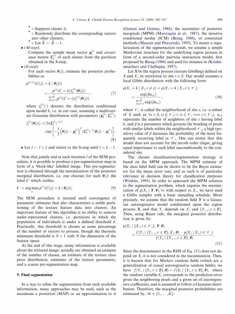
Note that jointly and at each iteration l of the SEM pro-cedure, it is possible to produce a pre-segmentation map inform of a ‘block-like’ labelled image. This pre-segmenta-tion is obtained through the maximization of the posteriormarginal distribution, i.e. one chooses for each hðjÞ thelabel k which verifies

k ¼ arg maxk

pðlÞðCðjÞ ¼ k j hðjÞÞ: ð9Þ

The SEM procedure is iterated until convergence ofparameter estimates that also characterizes a stable parti-tioning of the texture feature data into clusters. Animportant feature of this algorithm is its ability to removeunder-represented clusters, i.e. partitions in which thepopulation of individuals is under a defined threshold d.Practically, this threshold is chosen as some percentageof the number of vectors to process, though the theoreticminimum threshold is N þ 1 with N the dimension of thefeature space.

At the end of this stage, many information is availableabout the textured image: actually are obtained an estimateof the number of classes, an estimate of the texture classprior distribution, estimates of the texture parameters,and a coarse pre-segmentation map.

5. Final segmentation

In a way to refine the segmentation from such availableinformation, many approaches may be used, such as themaximum a posteriori (MAP) or an approximation to it

(Geman and Geman, 1984), the maximizer of posteriormarginals (MPM) (Marroquin et al., 1987), the iterativeconditional modes (ICM) (Besag, 1986), or contextualmethods (Masson and Pieczynski, 1993). To insure a regu-larization of the segmentation result, we assume a simpleMarkovian structure for the underlying region process inform of a second-order pairwise interaction model, firstproposed by Besag (1986) and used for instance in (Krishn-amachari and Chellappa, 1997).

Let X be the region process (texture labelling) defined onS and X s its restriction to site s 2 S. Our model assumes alocal Gibbs distribution with the following form:

pðX s ¼ k j X t; t 6¼ sÞ ¼ pðX s ¼ k j X t; t 2VsÞ

¼ expðbus;kÞPbKi¼1 expðbus;iÞ

; ð10Þ

where Vs is called the neighborhood of site s, i.e. a subsetof S such as 8s 2 S; ðs 62VsÞ ^ ðs 2Vt () t 2VsÞ, us;k

represents the number of neighbors of site s having labelk, and b is a parameter which governs the bonding of pixelswith similar labels within the neighborhood Vs; a high (po-sitive) value of b increases the probability of the most fre-quently occurring label in Vs. One can notice that thismodel does not account for the zeroth order clique, givingequal importance to each label unconditionally to the con-sidered site.

The chosen classification/segmentation strategy isbased on the MPM approach. The MPM estimate ofthe class label field can be shown to be the Bayes estima-tor for the mean error rate, and as such is of particularrelevance in decision theory for classification purposes(Winkler, 1995). In order to approach the MPM solutionto the segmentation problem, which requires the maximi-zation of pðX s j Y ; hÞ; 8s with respect to X s, we have useda Gibbs sampler with a basic annealing schedule. Moreprecisely, we assume that the random field Y is a Gauss-ian autoregressive model conditioned upon the regionprocess X, and that Y s depends on X s and fY s�r; r 2 Rg.Then, using Bayes rule, the marginal posterior distribu-tion is given by:

pðX s j fX t; t 2Vsg;Y ; hÞ

¼ f ðY s j fY s�r; r 2 Rg;X s; hÞ � pðX s j X t; t 2VsÞf ðY s j fY s�r; r 2 Rg; hÞ :

ð11Þ

Since the denominator in the RHS of Eq. (11) does not de-pend on X, it is not considered in the maximization. Then,it is known that for Markov random fields (which are ageneralization of causal autoregressive random fields), wehave f ðY s j fY r; r 2 Rg; hÞ ¼ f ðEs j fY r; r 2 Rg; hÞ, wherethe random variable Es corresponds to the prediction errorgiven the neighboring pixels and a given set of autoregres-sive coefficients, and is assumed to follow a Gaussian distri-bution. Therefore, the marginal posterior probabilities areestimated by, 8k 2 f1; . . . ;Kg:


pðX s ¼ k j fX t; t 2Vsg;Y ; hÞ

¼ 1

zffiffiffiffiffiffiffiffiffiffiffiffiffiffiffiffi2pr2ðkÞ

p exp �e2

s;k

2r2k

þ bus;k

!; ð12Þ

where es;k ¼ ðys � lkÞ �P

r2Rhr;kðys�r � lkÞ is the differencebetween the observation and its linear prediction over site sby the kth autoregressive model with parameter hk ¼½fhr;k; r 2 Rg; lk; r

2k �

T , and z is a normalizing constant. Notethat Eq. (12) is similar to Eq. (27) in (Krishnamachari andChellappa, 1997) except that the region conditional textureprocess was chosen as a Gauss–Markov random field bythe authors.

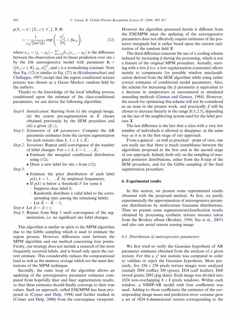
Thanks to the knowledge of the local labelling processconditioned upon the estimate of the class-conditionalparameters, we can derive the following algorithm:

Step 0: Initialization: Starting from (i) the original image,(ii) the coarse pre-segmentation in bK classesobtained previously by the SEM procedure and(iii) a given ðb; cÞ,

Step 1: Estimation of AR parameters: Compute the ARparameter estimates from the current segmentationfor each texture class k, 1 6 k 6 bK ;

Step 2: Iterations: Repeat until convergence of the numberof label changes: For s 2 S, k ¼ 1; . . . ; bK ;� Estimate the marginal conditional distribution

using (12);� Draw a new label for site s from (12);

Step 3:

� Estimate the prior distribution of each labelpðkÞ; k ¼ 1; . . . ; bK by empirical frequencies;� If pðkÞ is below a threshold d0 for some k

– Suppress class label k;– Randomly distribute a valid label to the corre-

sponding sites among the remaining labels;– Let bK bK � 1;

Step 4: Let b bþ c;Step 5: Repeat from Step 1 until convergence of the seg-

mentation, i.e. no significant site label changes.

This algorithm is similar in spirit to the MPM algorithmdue to the Gibbs sampling which is used to estimate theregion process. However, differences exist between theMPM algorithm and our method concerning four points.Firstly, our strategy does not include a research of the mostfrequently occurred labels, and is based only upon the cur-rent estimate. This considerably reduces the computationalload as well as the memory storage which are the main lim-itations of the MPM technique.

Secondly, the outer loop of the algorithm allows anupdating of the autoregressive parameter estimates com-puted from hopefully finer and finer segmentation results,so that these estimates should finally converge to their truevalues. Such an approach, called EM/MPM has been pro-posed in (Comer and Delp, 1994) and further studied in(Comer and Delp, 2000) from the convergence viewpoint.

However the algorithm presented herein is different fromthe EM/MPM since the updating of the autoregressiveparameters does not effectively require estimates of the pos-terior marginals but is rather based upon the current real-ization of the random field X.

The third difference concerns the use of a cooling schemeinduced by increasing b during the processing, which is nota feature of the original MPM procedure. Actually, start-ing with a low b (i.e. a low regularization constraint) allowsmainly to compensate for possible window misclassifi-cation derived from the SEM algorithm while using rathercorrect estimates of conditional model parameters. Also,the scheme for increasing the b parameter is equivalent toa decrease in temperature as encountered in simulatedannealing methods (Geman and Geman, 1984). However,the search for optimizing this scheme will not be consideredas an issue in the present work, and practically b will bechosen to increase linearly in the range [0.3,2.5], dependingon the size of the neighboring system used for the label pro-cess X.

The last difference is the fact that a class with a very fewnumber of individuals is allowed to disappear, in the sameway as it is in the first stage of our approach.

From a general – as well as practical – point of view, onecan easily see that there is much resemblance between thealgorithms proposed in the first and in the second stageof our approach. Indeed, both rely on the sampling of mar-ginal posterior distributions, either from the S-step of theSEM procedure, and for the Gibbs sampling of the finalsegmentation procedure.

6. Experimental results

In this section, we present some experimental resultsobtained with the proposed method. At first, we justifyexperimentally the approximation of autoregressive param-eter distributions by multivariate Gaussian distributions.Then we present some segmentation/classification resultsobtained by processing synthetic texture mosaics takenfrom the Brodatz album (Brodatz, 1956; Xia et al., 2007)and also one aerial remote sensing image.

6.1. Distribution of autoregressive parameters

We first tried to verify the Gaussian hypothesis of ARparameter estimates obtained from the analysis of a giventexture. For this a v2 test statistic was computed in orderto validate or reject the Gaussian hypothesis. More pre-cisely, five 256� 256 pixels texture images were analyzed(namely D84 (raffia); D9 (grass); D24 (calf leather); D68(wood grain); D92 (pig skin)). Each image was divided into1024 non-overlapping 8� 8 pixels windows. Within eachwindow, a NSHP-AR model with four coefficients wasused. Adding to those coefficients the estimates of the cor-responding image mean and prediction error variance gavea set of 1024 6-dimensional vectors corresponding to the


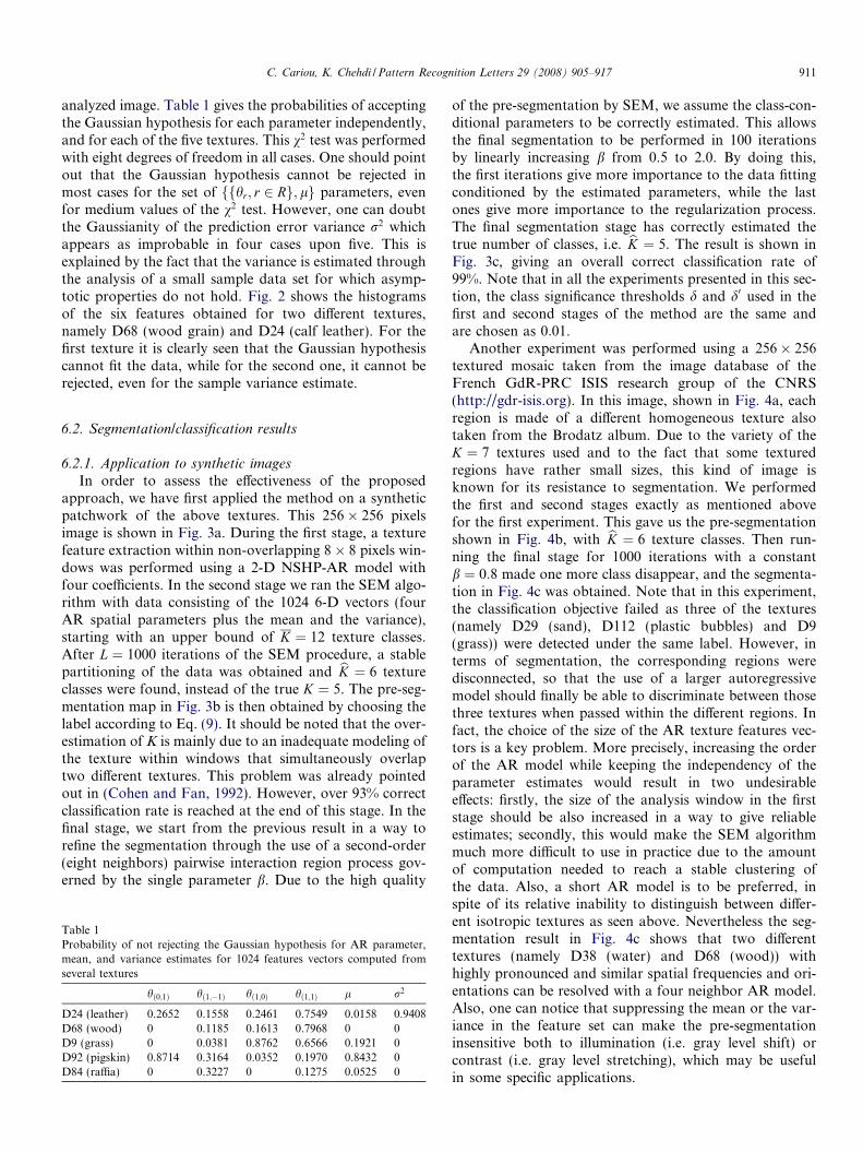
analyzed image. Table 1 gives the probabilities of acceptingthe Gaussian hypothesis for each parameter independently,and for each of the five textures. This v2 test was performedwith eight degrees of freedom in all cases. One should pointout that the Gaussian hypothesis cannot be rejected inmost cases for the set of ffhr; r 2 Rg; lg parameters, evenfor medium values of the v2 test. However, one can doubtthe Gaussianity of the prediction error variance r2 whichappears as improbable in four cases upon five. This isexplained by the fact that the variance is estimated throughthe analysis of a small sample data set for which asymp-totic properties do not hold. Fig. 2 shows the histogramsof the six features obtained for two different textures,namely D68 (wood grain) and D24 (calf leather). For thefirst texture it is clearly seen that the Gaussian hypothesiscannot fit the data, while for the second one, it cannot berejected, even for the sample variance estimate.

6.2. Segmentation/classification results

6.2.1. Application to synthetic images

In order to assess the effectiveness of the proposedapproach, we have first applied the method on a syntheticpatchwork of the above textures. This 256� 256 pixelsimage is shown in Fig. 3a. During the first stage, a texturefeature extraction within non-overlapping 8� 8 pixels win-dows was performed using a 2-D NSHP-AR model withfour coefficients. In the second stage we ran the SEM algo-rithm with data consisting of the 1024 6-D vectors (fourAR spatial parameters plus the mean and the variance),starting with an upper bound of K ¼ 12 texture classes.After L ¼ 1000 iterations of the SEM procedure, a stablepartitioning of the data was obtained and bK ¼ 6 textureclasses were found, instead of the true K ¼ 5. The pre-seg-mentation map in Fig. 3b is then obtained by choosing thelabel according to Eq. (9). It should be noted that the over-estimation of K is mainly due to an inadequate modeling ofthe texture within windows that simultaneously overlaptwo different textures. This problem was already pointedout in (Cohen and Fan, 1992). However, over 93% correctclassification rate is reached at the end of this stage. In thefinal stage, we start from the previous result in a way torefine the segmentation through the use of a second-order(eight neighbors) pairwise interaction region process gov-erned by the single parameter b. Due to the high quality

Table 1Probability of not rejecting the Gaussian hypothesis for AR parameter,mean, and variance estimates for 1024 features vectors computed fromseveral textures

hð0;1Þ hð1;�1Þ hð1;0Þ hð1;1Þ l r2

D24 (leather) 0.2652 0.1558 0.2461 0.7549 0.0158 0.9408D68 (wood) 0 0.1185 0.1613 0.7968 0 0D9 (grass) 0 0.0381 0.8762 0.6566 0.1921 0D92 (pigskin) 0.8714 0.3164 0.0352 0.1970 0.8432 0D84 (raffia) 0 0.3227 0 0.1275 0.0525 0

of the pre-segmentation by SEM, we assume the class-con-ditional parameters to be correctly estimated. This allowsthe final segmentation to be performed in 100 iterationsby linearly increasing b from 0.5 to 2.0. By doing this,the first iterations give more importance to the data fittingconditioned by the estimated parameters, while the lastones give more importance to the regularization process.The final segmentation stage has correctly estimated thetrue number of classes, i.e. bK ¼ 5. The result is shown inFig. 3c, giving an overall correct classification rate of99%. Note that in all the experiments presented in this sec-tion, the class significance thresholds d and d0 used in thefirst and second stages of the method are the same andare chosen as 0:01.

Another experiment was performed using a 256� 256textured mosaic taken from the image database of theFrench GdR-PRC ISIS research group of the CNRS(http://gdr-isis.org). In this image, shown in Fig. 4a, eachregion is made of a different homogeneous texture alsotaken from the Brodatz album. Due to the variety of theK ¼ 7 textures used and to the fact that some texturedregions have rather small sizes, this kind of image isknown for its resistance to segmentation. We performedthe first and second stages exactly as mentioned abovefor the first experiment. This gave us the pre-segmentationshown in Fig. 4b, with bK ¼ 6 texture classes. Then run-ning the final stage for 1000 iterations with a constantb ¼ 0:8 made one more class disappear, and the segmenta-tion in Fig. 4c was obtained. Note that in this experiment,the classification objective failed as three of the textures(namely D29 (sand), D112 (plastic bubbles) and D9(grass)) were detected under the same label. However, interms of segmentation, the corresponding regions weredisconnected, so that the use of a larger autoregressivemodel should finally be able to discriminate between thosethree textures when passed within the different regions. Infact, the choice of the size of the AR texture features vec-tors is a key problem. More precisely, increasing the orderof the AR model while keeping the independency of theparameter estimates would result in two undesirableeffects: firstly, the size of the analysis window in the firststage should be also increased in a way to give reliableestimates; secondly, this would make the SEM algorithmmuch more difficult to use in practice due to the amountof computation needed to reach a stable clustering ofthe data. Also, a short AR model is to be preferred, inspite of its relative inability to distinguish between differ-ent isotropic textures as seen above. Nevertheless the seg-mentation result in Fig. 4c shows that two differenttextures (namely D38 (water) and D68 (wood)) withhighly pronounced and similar spatial frequencies and ori-entations can be resolved with a four neighbor AR model.Also, one can notice that suppressing the mean or the var-iance in the feature set can make the pre-segmentationinsensitive both to illumination (i.e. gray level shift) orcontrast (i.e. gray level stretching), which may be usefulin some specific applications.

http://gdr-isis.org

0.6 0.8 1 1.2 1.40

100

200

300theta(0,1)

–0.4 –0.2 0 0.2 0.40

100

200

300theta(1,1)

–0.4 –0.2 0 0.2 0.4 0.60

100

200

300theta(1,0)

–0.6 –0.4 –0.2 0 0.2 0.40

100

200

300theta(1,1)

140 160 180 200 2200

100

200

300sample mean

–100 0 100 200 3000

100

200

300sample variance

0 0.2 0.4 0.6 0.8 10

50

100

150

200theta(0,1)

–0.4 –0.2 0 0.2 0.40

50

100

150

200theta(1,1)

–0.4 –0.2 0 0.2 0.4 0.60

50

100

150

200theta(1,0)

–0.4 –0.2 0 0.2 0.4 0.60

50

100

150

200theta(1,1)

110 120 130 140 1500

100

200

300sample mean

500 1000 1500 2000 25000

50

100

150

200sample variance

Fig. 2. Histograms of computed AR parameters for two different textures: (a) top: D68 (wood grain); (b) bottom: D24 (calf leather). Solid lines representthe Gaussian distributions obtained with sample mean and variance estimates and used to compute the v2 test.


6.2.2. Application to a large textured image database

To validate and compare our approach with other seg-mentation methods on a large image set, we have appliedit on the MIV image database described recently in (Xiaet al., 2007). This database is generated from 12 textures cho-sen from the Brodatz album, and a reference 256� 256image onto which are patched, in turn, four out of the 12 tex-tures. Therefore, 495 textured mosaics are generated by this

procedure. We have processed the whole image set under thefollowing conditions: for the SEM procedure, K ¼ 5,L ¼ 200, d ¼ 0:02, and for the classification refinementb 2 ½0:25; 1:70�, c ¼ 0:05 and d0 ¼ 0:01. The algorithm pro-posed in Section 5 was slightly modified for the stopping cri-terion: the b parameter was forced to follow, in 30 iterations,a sawtooth pattern from 0.25 to 1.70 during ten cycles, thusrequiring 300 iterations of the refinement procedure.

Fig. 3. (a) Top: original image; (b) middle: pre-segmentation by SEM; (c)bottom: final segmentation.

Fig. 4. (a) Top left: original image; (b) top right: pre-segmentation bySEM; (c) bottom left: final segmentation; (d) bottom right: boundarydetection.

Fig. 5. Reference image for texture segmentation assessment (from Xiaet al., 2007).


Fig. 5 shows the reference mosaic image used to build theMIV textured image database. Fig. 6 gives some partial andfinal segmentation results on the four examples (MIV1-4)also shown in (Xia et al., 2007). Table 2 extends comparedmisclassification percentages published in the same paper

with the results of our approach. The comparison includesthe Spatial Fuzzy Clustering (SFC) of Liew et al. (2003),the MRF-model-based method of Deng and Clausi(2005), and the Fuzzy Clustering of Spatial Patterns (FCSP)of which was shown in (Xia et al., 2007) to provide betterresults than the previous two methods. Out of the fourimage samples, only one gave a misclassification rategreater than the result given by the FCSP method. Theother misclassification rates show a clear improvement inthe classification objective by using our approach, with amean error rate of 9.30% compared to 10.26% by the FCSPmethod computed over the whole image dataset. Fig. 7depicts the frequency distribution of the correct classifica-tion rate. One can observe a concentration of the distribu-tion above 90% of correct classification, with a maximumat 99.26%. Nevertheless, some rates are far below the mean,and such situations occurred when the SEM procedure hasmerged the autoregressive features into a single cluster.

Table 2Percentage of misclassification on image set MIV (from Xia et al., 2007)

Image Texture components Methods

SFC Liew et al. (2003) MRF Deng and Clausi (2005) FCSP Proposed

MIV1 D4-D9-D16-D19 4.95 9.94 4.23 2.35

MIV2 D4-D16-D87-D110 6.98 12.18 5.30 1.69

MIV3 D9-D53-D77-D84 4.95 9.94 4.23 5.18MIV4 D9-D35-D55-D103 6.98 12.18 5.30 0.95

Average 495 Samples 12.10 17.38 10.26 9.30

Fig. 6. Texture segmentation results on the four test cases (MIV1–MIV4) available in (Xia et al., 2007). Left column: images to be segmented; middlecolumn: pre-segmentation by the SEM algorithm; right column: final segmentation.


The question of how our algorithm has reached the cor-rect class number K ¼ 4 has been also verified in this exper-iment. It appears that, after the SEM procedure, 33% of the

classification results have reached the correct class numberK ¼ 4. After the refinement procedure, this rate hasincreased to 48%, while 48% found bK ¼ 5 and only 4%

50 60 70 80 90 1000

5

10

15

20

25

30

35

40

45

Correct classification rate (%)

Cou

nts

Fig. 7. Histogram of correct classification percentage on the MIV imagedatabase.


found bK ¼ 3. However, a close analysis of the classificationresults shows our approach was able to detect some defectsin the texture homogeneity. For instance, several classifica-tion results independently and coherently exhibited oneelongated region with a separate label on the very left partof the D53 (oriental straw cloth) texture patch as shown inFig. 8. Actually, this result is due to the decrease of the localvariance at the left border of the original texture image.

6.2.3. Application to a remote sensing image

We have also tested our approach on a real world image,namely an aerial remote sensing image obtained with the

Fig. 8. Some examples of classifications of MIV textured mosaics givingbK ¼ 5 classes. First column: images to be segmented; second column: finalsegmentation. Texture D53 is the upper left on top mosaic and the lowerleft on the bottom mosaic.

CASI sensor (Compact Airborne Spectrographic Imager)available in our laboratory. This sensor is able to image aground scene, in a so-called ‘spatial mode’, in up to 12non-overlapping wavebands (at 1 m of ground resolution)ranging in the visible to near infrared spectrum (403–947 nm). Fig. 9a shows a 256� 256 CASI mono-band

Fig. 9. (a) Top: original image; (b) middle: pre-segmentation by SEM; (c)bottom: final segmentation.


image (at spectral band 587:5 5:1 nm) showing differentoriented patterns and textures. We have applied the pro-posed method to this image, taking K ¼ 20 as the upperbound of the number of classes. The SEM procedure wasrun for 1000 iterations, producing a pre-segmentationresult featuring 11 classes (see Fig. 9b). Then, the final seg-mentation has converged to nine classes which can be seenon Fig. 9c. The obtained result is satisfactory in the sensethat most of the prominent textures were correctly identi-fied, particularly the high frequency textures at the centerof the image.

7. Conclusion and perspectives

The unsupervised segmentation technique for texturedimages presented here works at two levels for statisticallyhomogeneous textured regions retrieval. The first levelattempts to extract texture features upon a window-based2-D AR modeling of the random field. The texture featuresare made of the within-window 2-D AR parameters, plusthe mean and the variance of the prediction error. Thesefeatures are then taken as data entries of the SEM algo-rithm, which can produce estimates of conditional distribu-tions and a coarse pre-segmentation map. As such, thisprocedure may be seen as a kind of pre-attentive visionprocedure. The second level allows one to classify eachpixel of the image on the basis of the previous parameterestimates and using a simple Gibbsian structure for theunderlying unobserved region process. This method offerssome advantages in comparison with others available inthe literature. Firstly it allows the estimation of the correctnumber of texture classes due to the use of the SEM algo-rithm. Secondly, the textured nature of homogeneousregions is taken into account via a modeling which is sim-ple in essence and in the few number of parameters that areneeded to describe them.

We would also point out the potential of using the auto-regressive modeling for region conditional textures. Moreprecisely, it is possible to use the prediction error as aboundary detector between regions. Since the predictionerror is readily available once the class-conditional autore-gressive parameters are estimated, it is quite simple toderive a boundary map based upon a thresholding scheme,for instance by computing for each site s the followingquantity:

T ðsÞ ¼XbKk¼1

pðX s ¼ k j fX t; t 2Vsg;Y ; hÞe2

s;k

2r2k

ð13Þ

and compare it with a defined threshold s. For example,Fig. 4d shows the resulting detected boundary mapobtained for s ¼ 3:0. We are currently working at theintegration of such information in conjunction with theregion-based segmentation in a way to refine the whole seg-mentation process.

Finally, it is important to note that other stochasticmodels for region-conditional texture may be used within

this framework, such as Gauss–Markov random fields(GMRFs) (Krishnamachari and Chellappa, 1997), moregeneral ones such as non-causal autoregressive-movingaverage models (NC-ARMA), or rotation and scale invari-ant stochastic models.

Acknowledgements

This work was supported by the Regional Council ofBrittany, France, and the European Regional Develop-ment Fund through the Interreg III-B (Atlantic Area) pro-ject PIMHAI No. 190.

References

Alata, O., Ramananjarasoa, C., 2005. Unsupervised textured imagesegmentation using 2-D quarter-plane autoregressive model with fourprediction supports. Pattern Recognition Lett. 26, 1069–1081.

Allili, M.S., Ziou, D., 2007. Globally adaptive region information forautomatic color texture image segmentation. Pattern Recognition Lett.28, 1946–1956.

Arivazhagan, S., Ganesan, L., 2003. Texture classification using wavelettransform. Pattern Recognition Lett. 24, 1513–1521.

Besag, J., 1986. On the statistical analysis of dirty pictures. J.R. Statist.Soc. B 48 (3), 259–302.

Bouman, C., Liu, B., 1991. Multiple resolution segmentation of texturedimages. IEEE Trans. Pattern Anal. Machine Intell. 13 (2), 99–113.

Box, G., Jenkins, G., 1970. Time Series Analysis: Forecasting andControl. Holden-Day, San Francisco.

Brodatz, P., 1956. Textures: A Photographic Album for Artists andDesigners. Dover, New-York.

Celeux, G., Diebolt, J., 1987. A probabilistic teacher algorithm foriterative maximum likelihood estimation. In: Classification andRelated Methods of Data Analysis. Amsterdam, Elsevier, North-Holland, pp. 617–623.

Celeux, G., Diebolt, J., 1992. A stochastic approximation type EM

algorithm for the mixture problem. Stochastics Stochastics Rep. 41,119–134.

Celeux, G., Chauveau, D., Diebolt, J., 1996. On stochastic versions of theEM algorithm. J. Statist. Comput. Simulat. 55, 287–314.

Champagnat, F., Goussard, Y., Idier, J., 1996. Unsupervised deconvolu-tion of sparse spike trains using stochastic approximation. IEEETrans. on Signal Process. 44 (12), 2988–2998.

Chehdi, K., Cariou, C., Kermad, C., 1994. Image segmentation andtexture classification using local thresholds and 2-D AR modeling. In:Proceedings EUSIPCO-94, Edinburgh, UK, September, pp. 30–33.

Cohen, F.S., Fan, Z., 1992. Maximum likelihood unsupervised texturedimage segmentation. CVGIP: Graphical Models and Image Processing54 (3), 239–251.

Comer, M.L., Delp, E.J., 1994. Parameter estimation and segmentation ofnoisy or textured images using the EM algorithm and MPM estimation.In: Proceedings International Conference on Image Processing, Aus-tin, Texas, vol. 3, pp. 650–654.

Comer, M.L., Delp, E.J., 1999. Segmentation of textured images using amultiresolution Gaussian autoregressive model. IEEE Trans. on ImageProcess. 8 (3), 408–420.

Comer, M.L., Delp, E.J., 2000. The EM/MPM algorithm for segmenta-tion of textured images: Analysis and further experimental results.IEEE Trans. on Image Process. 9 (10), 1731–1744.

Dempster, A.P., Laird, N.M., Rubin, D.B., 1977. Maximum likelihoodfrom incomplete data via the EM algorithm. J. Roy. Statist. Soc. Ser. B39, 1–38.

Deng, H., Clausi, D.A., 2005. Unsupervised segmentation of syntheticaperture radar ice imagery using a novel Markov random field model.IEEE Trans. Geosci. Remote Sensing 43 (3), 528–538.


Diebolt, J., Celeux, G., 1993. Asymptotic properties of a Stochastic EM

algorithm for estimating mixture proportions. Stochastic Mod. 9, 599–613.

Fogel, I., Sagi, D., 1989. Gabor filters as texture discriminator. Biol.Cyber. 61, 102–113.

Geman, S., Geman, D., 1984. Stochastic relaxation, Gibbs distributions,and the Bayesian restoration of images. IEEE Trans. Pattern Anal.Machine Intell. 6 (6), 721–741.

Hadamard, J., 1923. Lectures on Cauchy’s Problem in Linear PartialDifferential Equations. Yale University Press, New Haven, CT, USA.

Haralick, R.M., Shanmugam, K., Dinstein, I., 1973. Textural features forimage classification. IEEE Trans. Systems Man Cybernet. 3 (6), 610–621.

Hofmann, T., Puzicha, J., Buhmann, J.M., 1996. Unsupervised segmen-tation of textured images by pairwise data clustering. In: Proc.International Conference on Image Processing (ICIP’96), vol. 3.Lausanne, Switzerland.

Kay, S.M., 1988. Modern Spectral Analysis – Theory and Application.Prentice-Hall, Englewood Cliffs, NJ.

Kervrann, C., Heitz, F., 1995. A Markov random field model-basedapproach to unsupervised texture segmentation using local and globalspatial statistics. IEEE Trans. Image Process. 4 (6), 856–862.

Krishnamachari, S., Chellappa, R., 1997. Multiresolution Gauss–Markovrandom field models for texture segmentation. IEEE Trans. ImageProcess. 6 (2), 251–267.

Lakshmanan, S., Derin, H., 1989. Simultaneous parameter estimation andsegmentation of Gibbs random fields using simulated annealing. IEEETrans. Pattern Anal. Machine Intell. 11 (8), 799–813.

Li, F., Peng, J., 2004. Double random field models for remote sensingimage segmentation. Pattern Recognition Lett. 25 (1), 129–139.

Liew, A.W.-C., Leung, S.H., Lau, W.H., 2003. Segmentation of color lipimages by spatial fuzzy clustering. IEEE Trans. Fuzzy Syst. 11 (4),542–549.

Manjunath, B.S., Chellappa, R., 1991. Unsupervised texture segmentationusing Markov random field models. IEEE Trans. Pattern Anal.Machine Intell. 13 (5), 478–482.

Marroquin, J., Mitter, S., Poggio, T., 1987. Probabilistic solution of ill-posed problems in computational vision. J. Amer. Statist. Assoc. 82(397), 76–89.

Masson, P., Pieczynski, W., 1993. SEM algorithm and unsupervisedstatistical segmentation of satellite images. IEEE Trans. Geosci.Remote Sensing 31 (3), 618–633.

Melas, D.E., Wilson, S.P., 2002. Double Markov random fields andBayesian image segmentation. IEEE Trans. Acoustics, Speech SignalProcess. 50 (2), 357–365.

Mendel, J.M., 1995. Lessons in Estimation Theory for Signal ProcessingCommunication and Control. Prentice-Hall, Englewood-Cliffs, NJ.

Montiel, E., Aguado, A.S., Nixon, M.S., 2005. Texture classification viaconditional histograms. Pattern Recognition Lett. 26, 1740–1751.

Muneeswaran, K., Ganesan, L., Arumugam, S., Ruba Soundar, K., 2005.Texture classification with combined rotation and scale invariantwavelet features. Pattern Recognition 38, 1495–1506.

Muneeswaran, K., Ganesan, L., Arumugam, S., Ruba Soundar, K., 2006.Texture image segmentation using combined features from spatial andspectral distribution. Pattern Recognition Lett. 27, 755–764.

Ojala, T., Pietikinen, M., Harwood Pattern, D., 1996. A comparativestudy of texture measures with classification based on featureddistributions. Pattern Recognition 29 (1), 51–59.

Petrou, M., Sevilla, P.G., 2006. Image Processing: Dealing with Texture.Wiley.

Poggio, T., Koch, C., Torre, V., 1985. Computational vision andregularization theory. Nature 317, 314–319.

Reed, T.R., du Buf, H.J.M., 1993. A review of recent texture segmentationand feature extraction techniques. Graphical Models Image Process.57 (3), 359–372.

Reyes-Aldasoro, C.C., Bhalerao, A., 2006. The Bhattacharyya space forfeature selection and its application to texture segmentation. PatternRecognition 39, 812–826.

Richardson, S., Green, P.J., 1997. On Bayesian analysis of mixtures withan unknown number of components. J. Roy. Statist. Soc. Ser. B 59,731–792.

Wilson, S.P., Zerubia, J., 2001. Segmentation of textured satellite andaerial images by Bayesian inference and Markov random fields,INRIA research report, RR-4336, December 2001.

Winkler, G., 1995. Image analysis, random fields and dynamic MonteCarlo methods. In: Karatzas, I., Yor, M. (Eds.), Applications ofMathematics. Springer-Verlag.

Xia, Y., Feng, D., Zhao, R., 2006. Morphology-based multifractalestimation for texture segmentation. IEEE Trans. Image Process. 15(3), 614–623.

Xia, Y., Feng, D., Wang, T., Zhao, R., Zhang, Y., 2007. Imagesegmentation by clustering of spatial patterns. Pattern RecognitionLett. 28 (12), 1548–1555.

Zhang, J., Modestino, J.W., 1990. A model-fitting approach to clustervalidation with application to stochastic model-based image seg-mentation. IEEE Trans. Pattern Anal. Machine Intell. 12 (10),1009–1017.

Zhang, J., Modestino, J.W., Langan, D.A., 1994. Maximum-likehoodparameter estimation for unsupervised stochastic model-based imagesegmentation. IEEE Trans. Image Process. 3 (4), 404–420.

unsupervised texture segmentation/classification using 2-d autoregressive modeling and the...

Documents