unterlagen zur vorlesung - haw · pdf filedie vorlesung flugmechanik 1 wird seit ss99...

Unterlagenzur Vorlesung

Flugmechanik 1

Prof. Dr.-Ing. Dieter Scholz, MSME

2 Flight Mechanics 1

Prof. Dr.-Ing. Dieter Scholz HAW H a m b u r g FACHBEREICH FAHRZEUGTECHNIK UND FLUGZEUGBAU

Prof. Dr.-Ing. Dieter Scholz, MSME

Hochschule für Angewandte Wissenschaften Hamburg

Fachbereich Fahrzeugtechnik und Flugzeugbau

Berliner Tor 5

D - 20099 Hamburg

Tel.: 040 - 709 716 46

E-Mail: [email protected]

WWW: http://ProfScholz.de

Flight Mechanics 1 3


Vorwort

Flugmechanik 1 an der HAW Hamburg beschäftigt sich schwerpunktmäßig mit Flugleistungen

(aircraft performance) darüber hinaus wird ein Einstieg in Flugeigenschaftsrechnungen (aircraft

stability and control) gegeben.

Die Vorlesung Flugmechanik 1 wird seit SS99 durchgeführt basierend auf dem Flugmechanik-

Skript der University of Limerick, Department of Mechanical & Aeronautical Engineering.

Der Autor des Skripts ist Trevor Young. Mr. Trevor Young ist an der University of Limerick

verantwortlich für die Organisation der Kurse im Flugzeugbau. Er lehrt die Fächer Flugmechanik und

Flugzeugentwurf.

Die hier vorliegenden Unterlagen sind als Ergänzung gedacht zum Skript. Die Numerierung der

Unterlagen entspricht der Numerierung im Skript. Ich erstelle die Unterlagen in englisch, da sie

auch international genutzt werden.



Contents

1 Introduction to Flight Mechanics and the ISA .................................................................. 5

1.1 Equations for the International Standard Atmosphere ..................................................... 7

1.2 Height Scales and Conversions ..................................................................................... 8

1.3 Aircraft Speed Definitions and Conversions ................................................................. 10

1.4 Air Temperature ......................................................................................................... 13

1.5 Rules of Thumb ........................................................................................................... 14

3 Aircraft Drag and Drag Power ......................................................................................... 15

4 Powerplant Performance ................................................................................................... 16

4.1 Thrust and Efficency ................................................................................................... 16

4.2 Propeller Efficiency ..................................................................................................... 19

5 Level, Climbing and Descending Flight ........................................................................... 23

5.1 Climb and Climb Schedules ........................................................................................ 23

5.2 Time to Climb ............................................................................................................ 25

5.3 Approximate Climb Calculation .................................................................................. 25

6 Stall, Speed Stability, Turning Performance .................................................................... 27

References ................................................................................................................................... 28

Appendix

A Derivations .................................................................................................................. 29



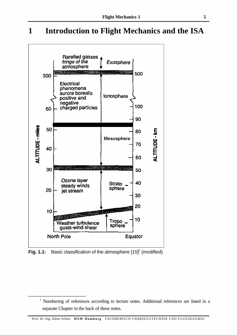
1 Introduction to Flight Mechanics and the ISA

Fig. 1.1: Basic classification of the atmosphere [15]1 (modified)

1 Numbering of references according to lecture notes. Additional references are listed in a

separate Chapter in the back of these notes.



Fig. 1.2: Temperature distribution in the standard atmosphere (ANDERSON 1989)



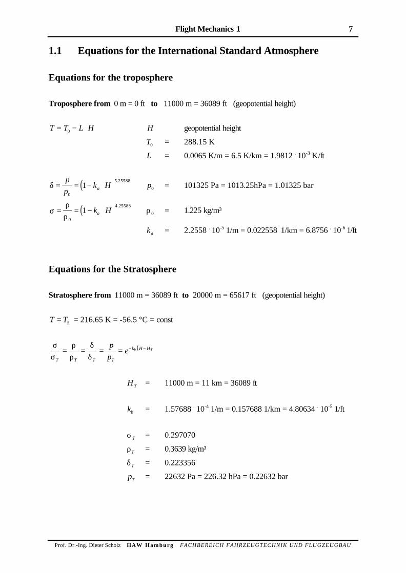
1.1 Equations for the International Standard Atmosphere

Equations for the troposphere

Troposphere from 0 m = 0 ft to 11000 m = 36089 ft (geopotential height)

T T L H= − ⋅0 H geopotential height

T0 = 288.15 K

L = 0.0065 K/m = 6.5 K/km = 1.9812 . 10-3 K/ft

( )δ = = − ⋅pp

k Ha0

5 255881

.p0 = 101325 Pa = 1013.25hPa = 1.01325 bar

( )σρρ

= = − ⋅0

4 255881 k Ha

.ρ0 = 1.225 kg/m³

ka = 2.2558 . 10-5 1/m = 0.022558 1/km = 6.8756 . 10-6 1/ft

Equations for the Stratosphere

Stratosphere from 11000 m = 36089 ft to 20000 m = 65617 ft (geopotential height)

T TS= = 216.65 K = -56.5 °C = const

( )σσ

ρρ

δδT T T T

k H Hpp

e b T= = = = − ⋅ −

HT = 11000 m = 11 km = 36089 ft

kb = 1.57688 . 10-4 1/m = 0.157688 1/km = 4.80634 . 10-5 1/ft

σT = 0.297070

ρT = 0.3639 kg/m³

δT = 0.223356

pT = 22632 Pa = 226.32 hPa = 0.22632 bar



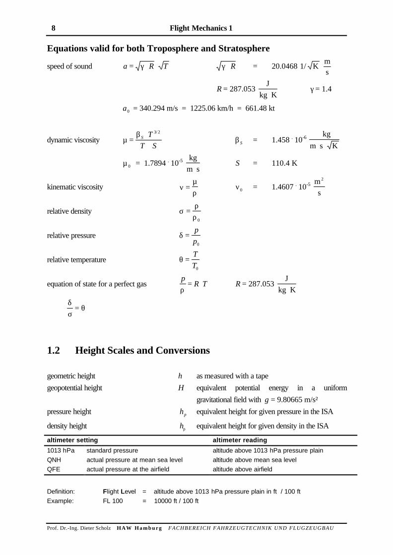
Equations valid for both Troposphere and Stratosphere

speed of sound a R T= ⋅ ⋅γ γ ⋅ R = 20.0468 sm

K/1 ⋅

R = 287.053 J

kg K⋅γ = 1.4

a0 = 340.294 m/s = 1225.06 km/h = 661.48 kt

dynamic viscosity µβ

=⋅+

S TT S

3 2/

βS = 1.458 . 10-6 kg

m s K⋅ ⋅

µ 0 = 1.7894 . 10-5 kg

m s⋅S = 110.4 K

kinematic viscosity νµρ

= ν0 = 1.4607 . 10-5 m

s

2

relative density σρρ

=0

relative pressure δ =pp0

relative temperature θ =TT0

equation of state for a perfect gasp

R Tρ

= ⋅ R = 287.053 J

kg K⋅

δσ

θ=

1.2 Height Scales and Conversions

geometric height h as measured with a tape

geopotential height H equivalent potential energy in a uniform

gravitational field with g = 9.80665 m/s²

pressure height hp equivalent height for given pressure in the ISA

density height hρ equivalent height for given density in the ISA

altimeter setting altimeter reading

1013 hPa standard pressure altitude above 1013 hPa pressure plain

QNH actual pressure at mean sea level altitude above mean sea level

QFE actual pressure at the airfield altitude above airfield

Definition: Flight Level = altitude above 1013 hPa pressure plain in ft / 100 ft

Example: FL 100 = 10000 ft / 100 ft



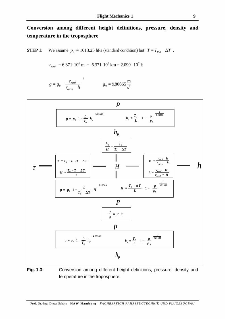
Conversion among different height definitions, pressure, density and

temperature in the troposphere

STEP 1: We assume p0 = 1013.25 hPa (standard condition) but T T TISA= + ∆ .

rearth = 6.371. 106 m = 6.371. 103 km = 2.090 . 107 ft

g gr

r hearth

earth

= ⋅+

0

2

g0 980665= .m

s2

T hH

r hr h

earth

earth=

⋅+

hr H

r Hearth

earth=

⋅−

THLTT ∆+⋅−= 0

LTTTH ∆+−

= 0

p pLT hp= − ⋅

0

0

5 25588

1.

hTL

ppp = ⋅ −

0

0

1

5 25588

1.

p

hp

hH

TT T

p =+

0

0 ∆

H

p pL

T TH= −

+⋅

0

0

5 2 5 5 8 8

1∆

.

HT T

Lpp

=+

⋅ −

0

0

1

5 25588

1∆ .

pp

R Tρ

= ⋅

ρ

ρ ρ ρ= − ⋅

0

0

4 2 5 5 8 8

1LT

h.

hTLρ

ρρ

= ⋅ −

0

0

14 25588

1.

hρ

T hH

r hr h

earth

earth=

⋅+

hr H

r Hearth

earth=

⋅−

THLTT ∆+⋅−= 0

LTTTH ∆+−

= 0

p pLT hp= − ⋅

0

0

5 25588

1.

hTL

ppp = ⋅ −

0

0

1

5 25588

1.

p

hp

hH

TT T

p =+

0

0 ∆

H

p pL

T TH= −

+⋅

0

0

5 2 5 5 8 8

1∆

.

HT T

Lpp

=+

⋅ −

0

0

1

5 25588

1∆ .

pp

R Tρ

= ⋅

ρ

ρ ρ ρ= − ⋅

0

0

4 2 5 5 8 8

1LT

h.

hTLρ

ρρ

= ⋅ −

0

0

14 25588

1.

hρ

Fig. 1.3: Conversion among different height definitions, pressure, density and




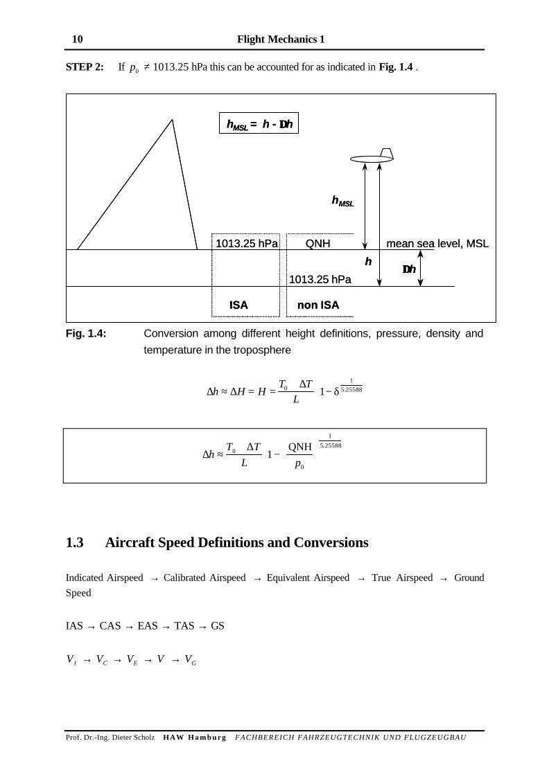
STEP 2: If p0 ≠ 1013.25 hPa this can be accounted for as indicated in Fig. 1.4 .

mean sea level, MSL

non ISAISA

1013.25 hPa

QNH1013.25 hPa

∆∆hh

hMSL

hMSL = h - ∆∆h

mean sea level, MSL

non ISAISA

1013.25 hPa

QNH1013.25 hPa

∆∆hh

hMSL

hMSL = h - ∆∆h

Fig. 1.4: Conversion among different height definitions, pressure, density and


∆ ∆∆

h H HT T

L≈ = =

+−

0

1

5 255881 δ .

∆∆

hT T

L p≈

+−

0

0

1

5 25588

1QNH .

1.3 Aircraft Speed Definitions and Conversions

Indicated Airspeed → Calibrated Airspeed → Equivalent Airspeed → True Airspeed → Ground

Speed

IAS → CAS → EAS → TAS → GS

V I → VC → VE → V → VG



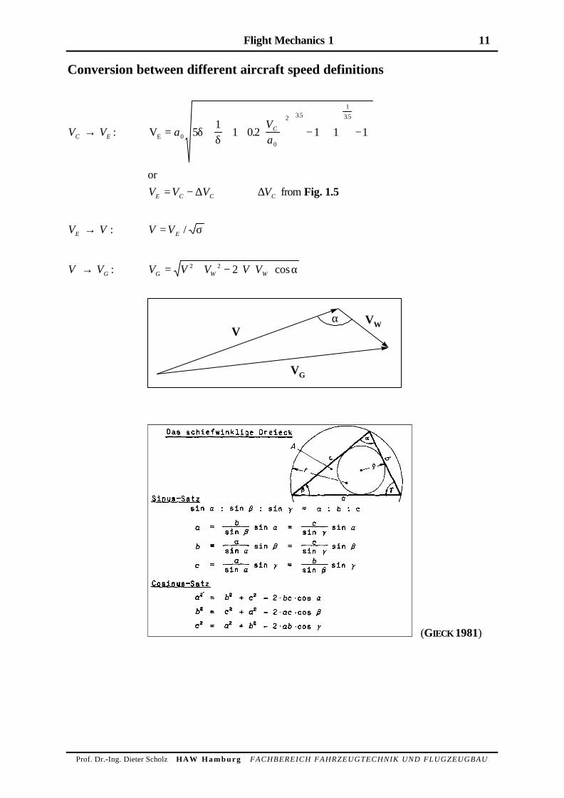
Conversion between different aircraft speed definitions

VC → VE : VE = +

−

+

−

aVa

C0

0

2 3 51

3 5

51

1 02 1 1 1δδ

.

. .

or

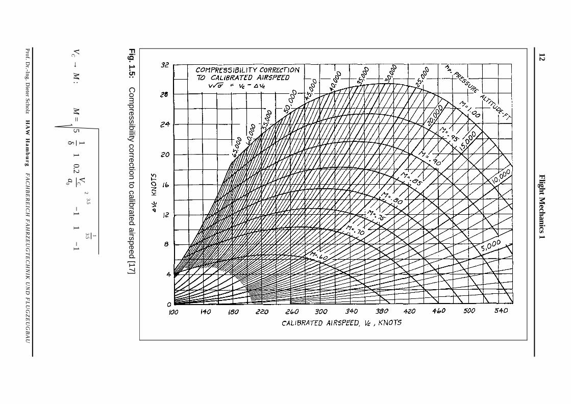
V V VE C C= − ∆ ∆VC from Fig. 1.5

VE → V : V VE= / σ

V → VG : V V V V VG W W= + − ⋅ ⋅ ⋅2 2 2 cosα

V

VG

VWα

(GIECK 1981)

12F

light Mechanics 1

Prof. D

r.-Ing. Dieter S

cholz HA

W H

am

bu

rg F

AC

HB

ER

EIC

H F

AH

RZ

EU

GT

EC

HN

IK U

ND

FL

UG

ZE

UG

BA

U

Fig

. 1.5:C

ompressibility correction to calibrated airspeed [17]

VC →

M:

MVa

C=

+

−

+

−

51

10

21

11

0

23

5135

δ.

..



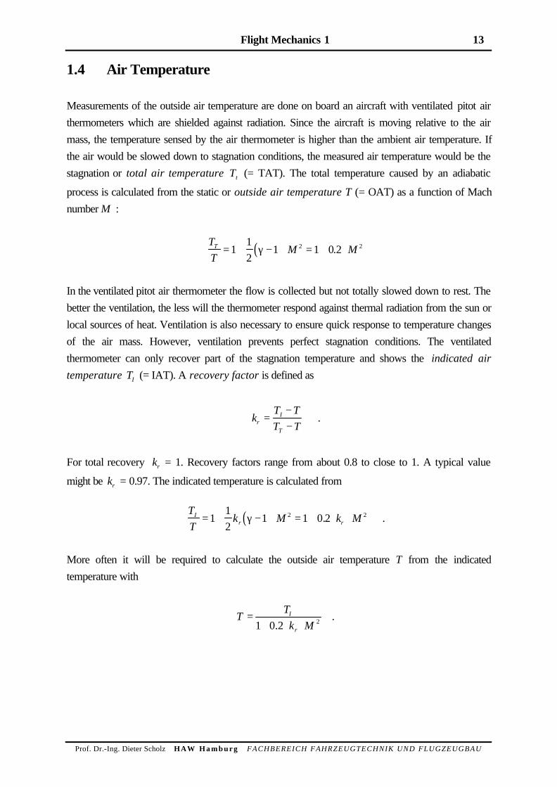
1.4 Air Temperature

Measurements of the outside air temperature are done on board an aircraft with ventilated pitot air

thermometers which are shielded against radiation. Since the aircraft is moving relative to the air

mass, the temperature sensed by the air thermometer is higher than the ambient air temperature. If

the air would be slowed down to stagnation conditions, the measured air temperature would be the

stagnation or total air temperature Tt (= TAT). The total temperature caused by an adiabatic

process is calculated from the static or outside air temperature T (= OAT) as a function of Mach

number M :

( )TT

M MT = + − ⋅ = + ⋅11

21 1 0 22 2γ .

In the ventilated pitot air thermometer the flow is collected but not totally slowed down to rest. The

better the ventilation, the less will the thermometer respond against thermal radiation from the sun or

local sources of heat. Ventilation is also necessary to ensure quick response to temperature changes

of the air mass. However, ventilation prevents perfect stagnation conditions. The ventilated

thermometer can only recover part of the stagnation temperature and shows the indicated airtemperature TI (= IAT). A recovery factor is defined as

kT TT Tr

I

T

=−−

.

For total recovery kr = 1. Recovery factors range from about 0.8 to close to 1. A typical value

might be kr = 0.97. The indicated temperature is calculated from

( )TT

k M k MIr r= + − ⋅ = + ⋅ ⋅1

1

21 1 0 22 2γ . .

More often it will be required to calculate the outside air temperature T from the indicated

temperature with

22.01 MkTT

r

I

⋅⋅+= .



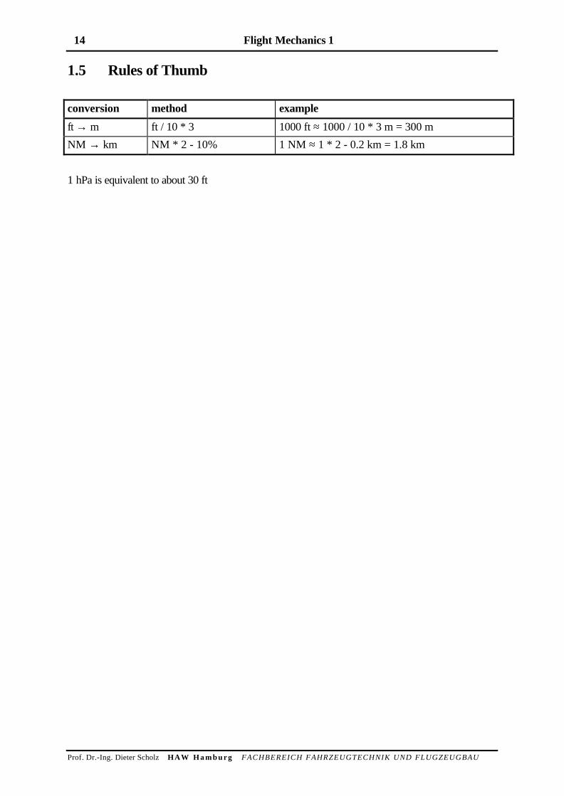
1.5 Rules of Thumb

conversion method example

ft → m ft / 10 * 3 1000 ft ≈ 1000 / 10 * 3 m = 300 m

NM → km NM * 2 - 10% 1 NM ≈ 1 * 2 - 0.2 km = 1.8 km

1 hPa is equivalent to about 30 ft



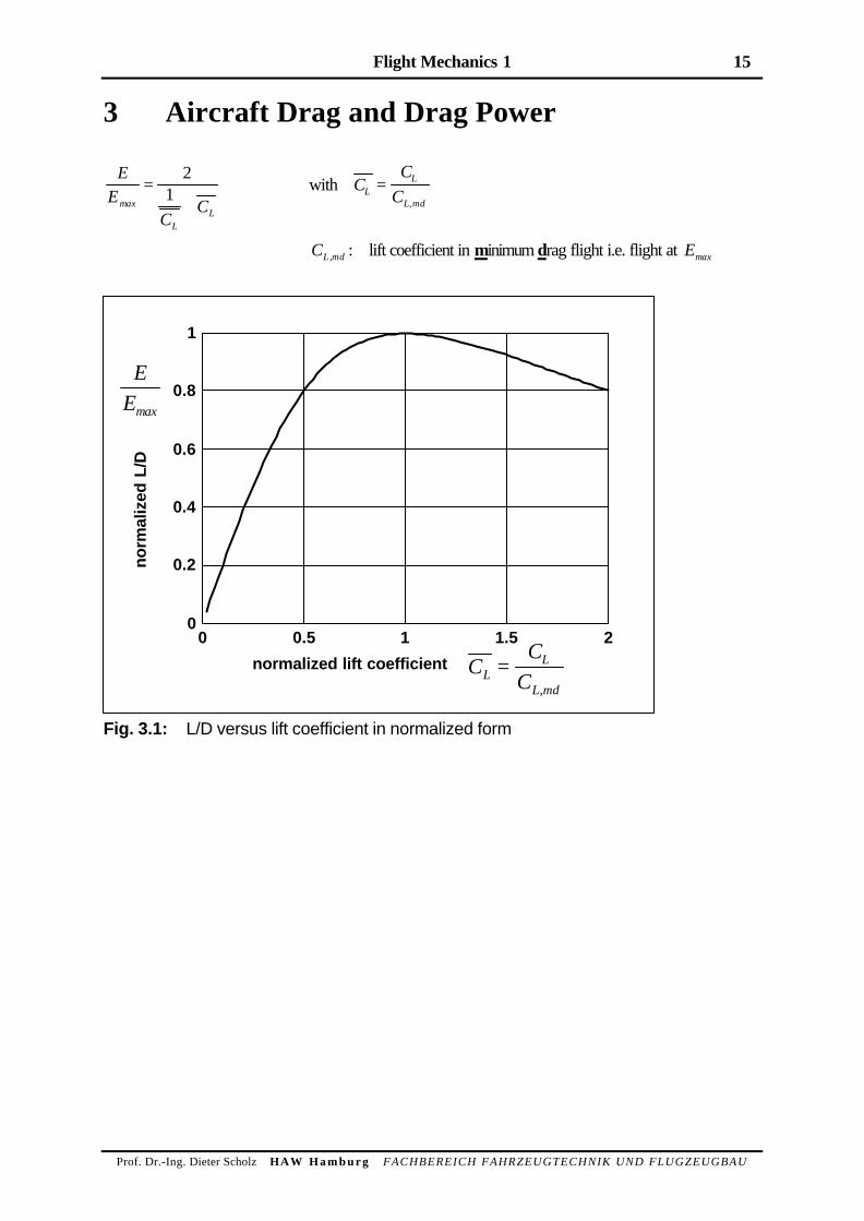
3 Aircraft Drag and Drag Power

EE

CCmax

LL

=+

21 with C

CCL

L

L md

=,

CL md, : lift coefficient in minimum drag flight i.e. flight at Emax

0

0.2

0.4

0.6

0.8

1

0 0.5 1 1.5 2

no

rmal

ized

L/D

normalized lift coefficient CC

CLL

L md=

,

EEmax

Fig. 3.1: L/D versus lift coefficient in normalized form



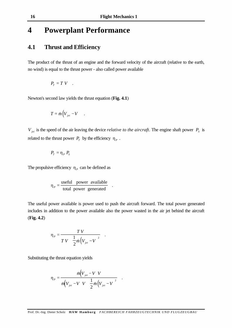
4 Powerplant Performance

4.1 Thrust and Efficiency

The product of the thrust of an engine and the forward velocity of the aircraft (relative to the earth,

no wind) is equal to the thrust power - also called power available

P T VT = .

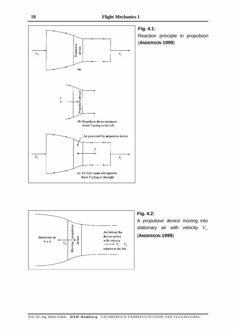
Newton's second law yields the thrust equation (Fig. 4.1)

( )T m V Vjet= −& .

V jet is the speed of the air leaving the device relative to the aircraft. The engine shaft power PS is

related to the thrust power PT by the efficiency ηP .

P PT P S= η

The propulsive efficiency ηP can be defined as

ηP =useful power available

total power generated .

The useful power available is power used to push the aircraft forward. The total power generated

includes in addition to the power available also the power wasted in the air jet behind the aircraft

(Fig. 4.2)

( )ηP

jet

T V

T V m V V=

+ −1

2

2&

.

Substituting the thrust equation yields

( )( ) ( )

ηP

jet

jet jet

m V V V

m V V V m V V=

−

− + −

&

& &1

2

2 .



Dividing numerator and denominator by ( )&m V V Vjet − :

( )21

21

1

1

21

1

1

−+=

−+

=

VV

VVV jetjet

Pη .

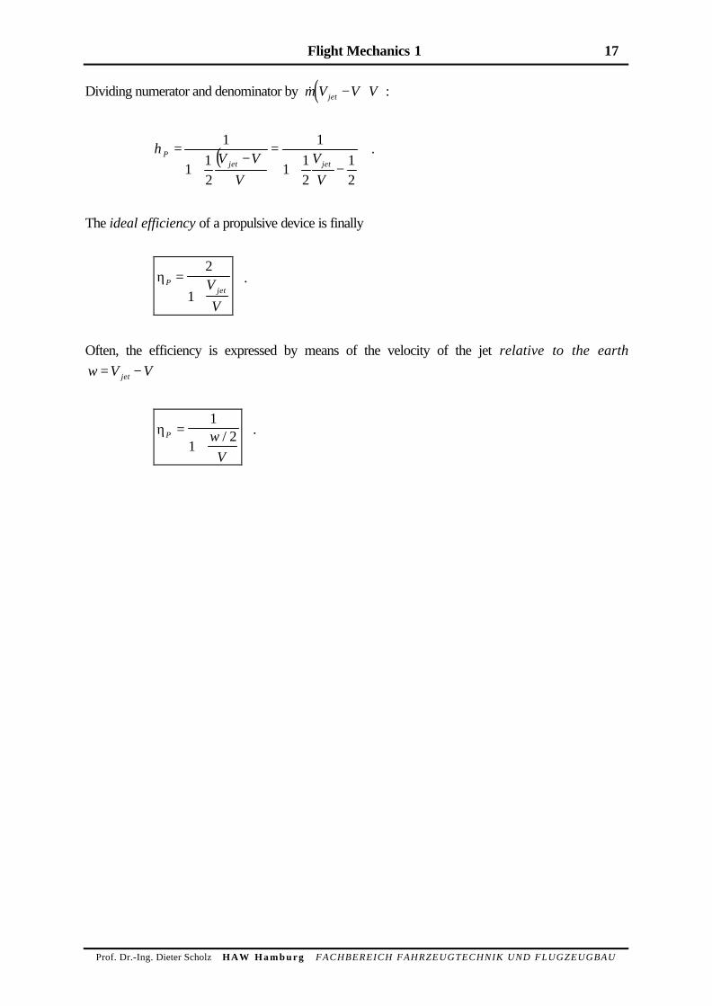
The ideal efficiency of a propulsive device is finally

ηPjetV

V

=+

2

1 .

Often, the efficiency is expressed by means of the velocity of the jet relative to the earthw V Vjet= −

ηP wV

=+

1

12/ .



Fig. 4.1:

Reaction principle in propulsion

(ANDERSON 1999)

Fig. 4.2:

A propulsive device moving into

stationary air with velocity V∞

(ANDERSON 1999)



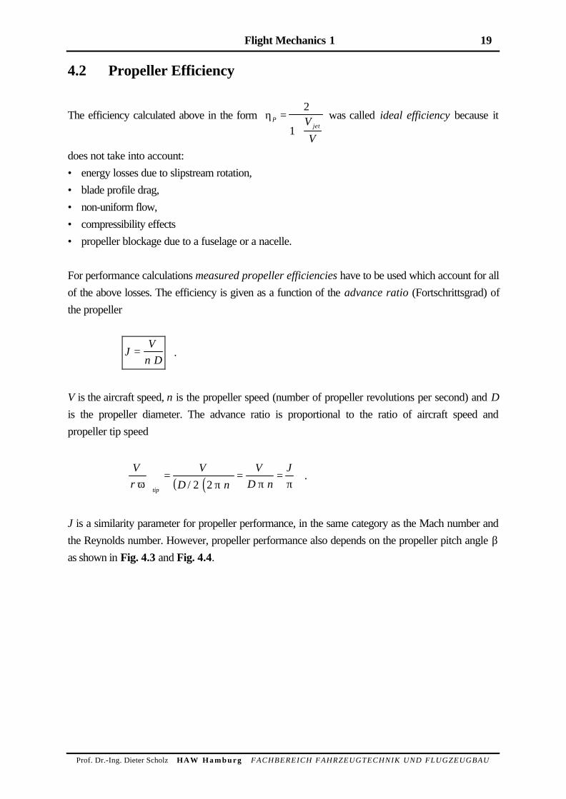
4.2 Propeller Efficiency

The efficiency calculated above in the form ηPjetV

V

=+

2

1 was called ideal efficiency because it

does not take into account:

• energy losses due to slipstream rotation,

• blade profile drag,

• non-uniform flow,

• compressibility effects

• propeller blockage due to a fuselage or a nacelle.

For performance calculations measured propeller efficiencies have to be used which account for all

of the above losses. The efficiency is given as a function of the advance ratio (Fortschrittsgrad) of

the propeller

JV

n D= .

V is the aircraft speed, n is the propeller speed (number of propeller revolutions per second) and Dis the propeller diameter. The advance ratio is proportional to the ratio of aircraft speed and

propeller tip speed

( )( )Vr

VD n

VD n

J

tipω π π π

= = =

/ 2 2 .

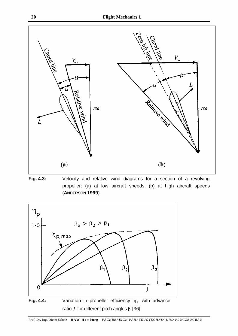
J is a similarity parameter for propeller performance, in the same category as the Mach number and

the Reynolds number. However, propeller performance also depends on the propeller pitch angle βas shown in Fig. 4.3 and Fig. 4.4.



Fig. 4.3: Velocity and relative wind diagrams for a section of a revolving

propeller: (a) at low aircraft speeds, (b) at high aircraft speeds

(ANDERSON 1999)

Fig. 4.4: Variation in propeller efficiency ηP with advance

ratio J for different pitch angles β [36]



From Fig. 4.3 follows that the propeller has to be twisted. The propeller pitch angle has to be a

function of the propeller radius. Propeller charts (like Fig. 4.4) must refer to a pitch angle β at a

specific radius as e.g. 075. ⋅ R .

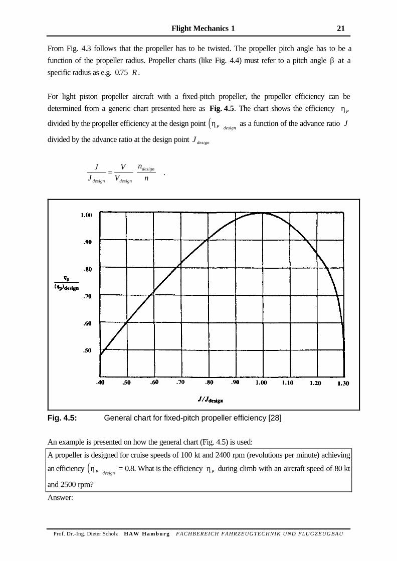
For light piston propeller aircraft with a fixed-pitch propeller, the propeller efficiency can be

determined from a generic chart presented here as Fig. 4.5. The chart shows the efficiency ηP

divided by the propeller efficiency at the design point ( )ηP design as a function of the advance ratio J

divided by the advance ratio at the design point J design

JJ

VV

nndesign design

design= ⋅ .

Fig. 4.5: General chart for fixed-pitch propeller efficiency [28]

An example is presented on how the general chart (Fig. 4.5) is used:

A propeller is designed for cruise speeds of 100 kt and 2400 rpm (revolutions per minute) achieving

an efficiency ( )ηP design = 0.8. What is the efficiency ηP during climb with an aircraft speed of 80 kt

and 2500 rpm?

Answer:



JJ

VV

nndesign design

design= ⋅ = ⋅ =80

10024002500

0 768.

and with Fig. 4.5

( ) ( )η ηη

ηP P designP

P design

= ⋅ = ⋅ =08 087 0 7. . . .

Thrust is calculated from

TP

VP S=

⋅η .

The static thrust at the beginning of the take-off run can not be calculated from the above equation

because at V = 0 also J = 0 and hence ηP = 0. So we have a case 0/0. "As a rough approximation

it can be assumed that the static thrust is about equal to the thrust at 50 knots for the fixed-pitch

propeller." [28]



5 Level, Climbing and Descending Flight

5.1 Climb and Climb Schedules

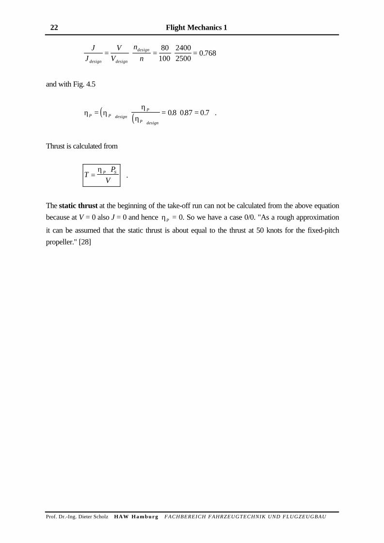
Fig. 5.1:

Maximum rate of climb

and maximum climb

angle for different climb

performance

(LUFTHANSA 1988)

For positive climb gradients the speed for best rate of climb is above that speed for best climb angle

(Fig. 5.1). With decreasing climb performance, the speeds for best angle and best rate of climb

come together. Finally, in the range of negative rate of climb, the speed for best angle is above that

for best descent rate. Hence, in descending flight, range is maximized with a speed above that for

maximum time aloft.

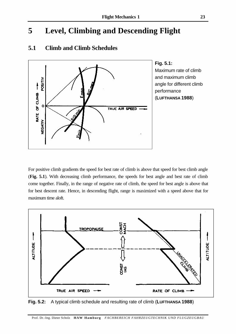
Fig. 5.2: A typical climb schedule and resulting rate of climb (LUFTHANSA 1988)



A typical climb schedule (Fig. 5.2-left) consists of three parts:

1. In the lower part of the troposphere, the climb is performed at constant IAS. This is done up to a

point where a certain Mach number is reached.

2. It follows a constant Mach number climb in the troposphere results in a decreasing true air speed.

3. In the stratosphere, the continued constant Mach number climb results in a flight at constant true

air speed.

In part 1, the climb rate is about 25% below the theoretical values for unaccelerated climb. In part 2,

the climb rate is about 9% above the theoretical values for unaccelerated climb. During transition

from constant IAS flight to constant Mach number flight, an increase in climb rate of up to 30% can

be observed LUFTHANSA 1988. In part 3, climb with constant true air speed results in an

unaccelerated climb.

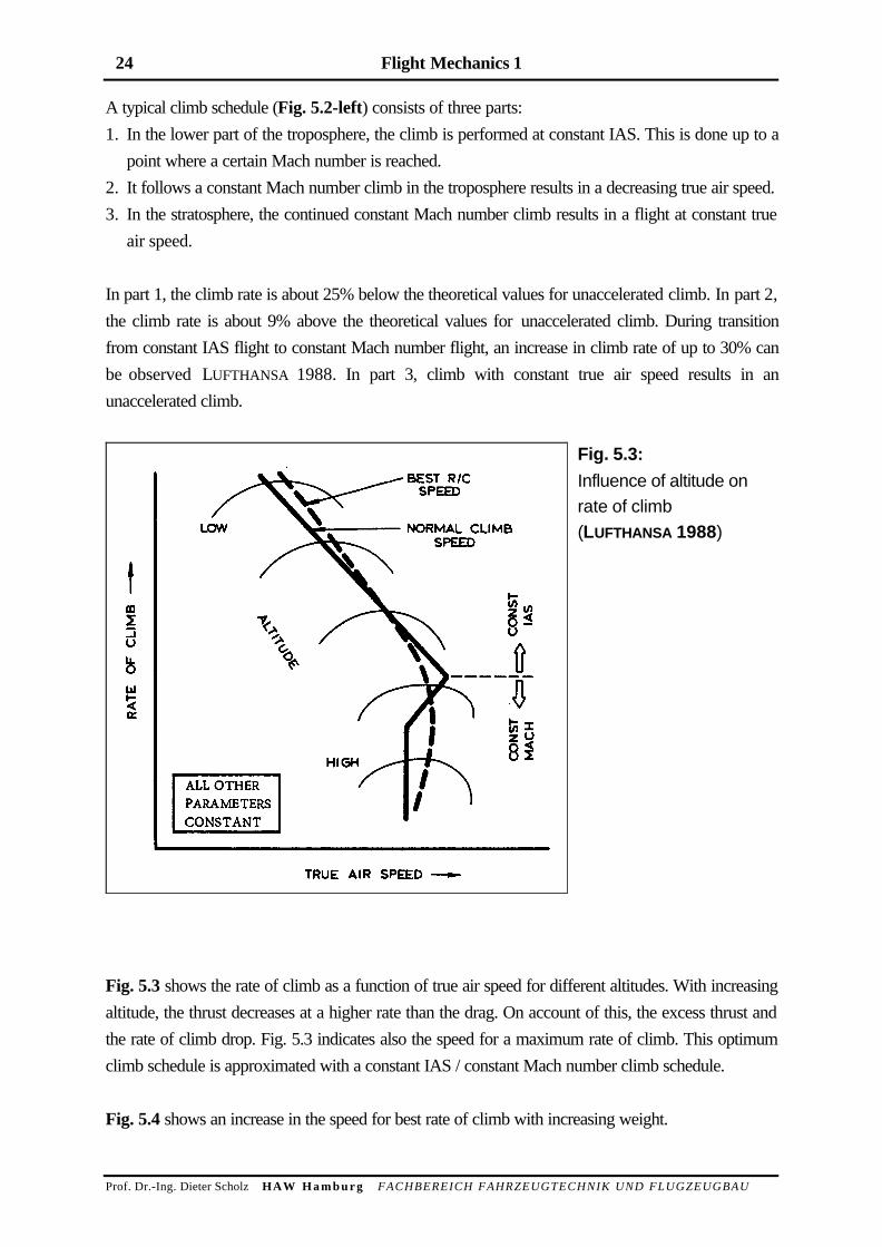
Fig. 5.3:

Influence of altitude on

rate of climb

(LUFTHANSA 1988)

Fig. 5.3 shows the rate of climb as a function of true air speed for different altitudes. With increasing

altitude, the thrust decreases at a higher rate than the drag. On account of this, the excess thrust and

the rate of climb drop. Fig. 5.3 indicates also the speed for a maximum rate of climb. This optimum

climb schedule is approximated with a constant IAS / constant Mach number climb schedule.

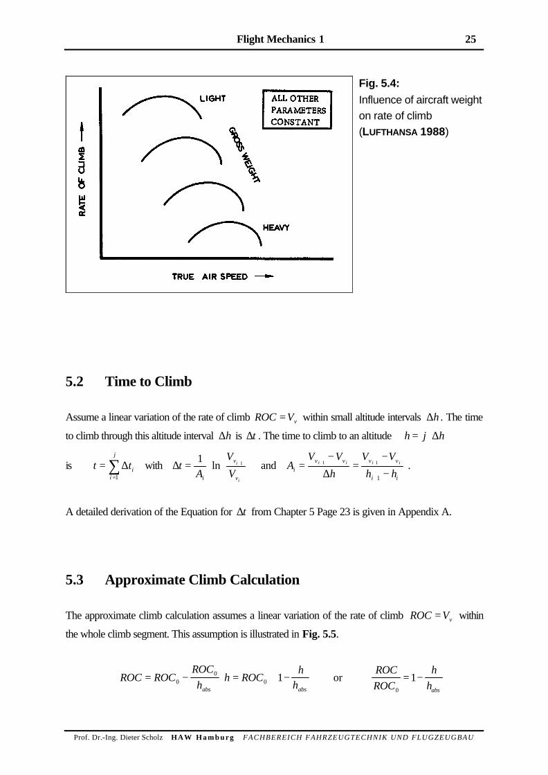
Fig. 5.4 shows an increase in the speed for best rate of climb with increasing weight.



Fig. 5.4:

Influence of aircraft weight

on rate of climb

(LUFTHANSA 1988)

5.2 Time to Climb

Assume a linear variation of the rate of climb ROC Vv= within small altitude intervals ∆h . The time

to climb through this altitude interval ∆h is ∆t . The time to climb to an altitude h j h= ⋅∆

is t tii

j

==∑∆

1

with ∆tA

VVi

v

v

i

i

= ⋅

+11ln and A

V Vh

V Vh hi

v v v v

i i

i i i i=−

=−−

+ +

+

1 1

1∆ .

A detailed derivation of the Equation for ∆t from Chapter 5 Page 23 is given in Appendix A.

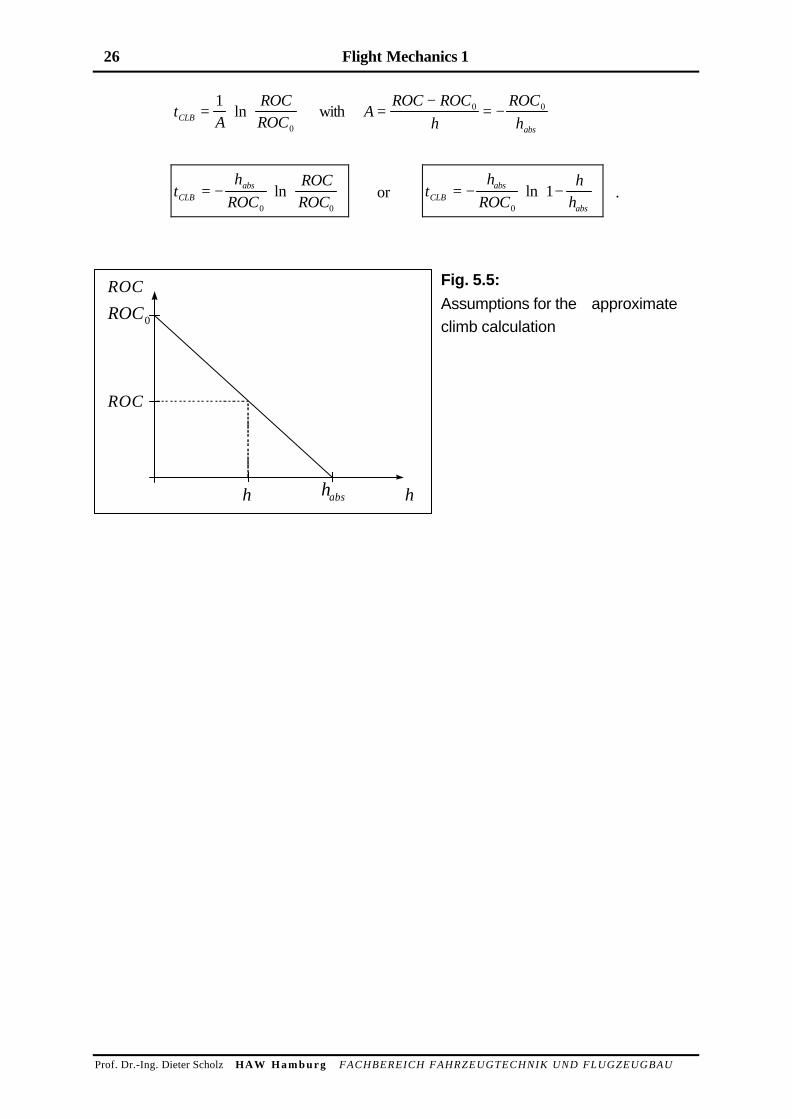
5.3 Approximate Climb Calculation

The approximate climb calculation assumes a linear variation of the rate of climb ROC Vv= within

the whole climb segment. This assumption is illustrated in Fig. 5.5.

ROC ROCROCh

h ROCh

habs abs

= − ⋅ = ⋅ −

0

00 1 or

ROCROC

hhabs0

1= −



tA

ROCROCCLB = ⋅

1

0

ln with AROC ROC

hROChabs

=−

= −0 0

th

ROCROCROCCLB

abs= − ⋅

0 0

ln or th

ROCh

hCLBabs

abs

= − ⋅ −

0

1ln .

Fig. 5.5:

Assumptions for the approximate

climb calculation

habsh

ROC0

ROC

h

ROC



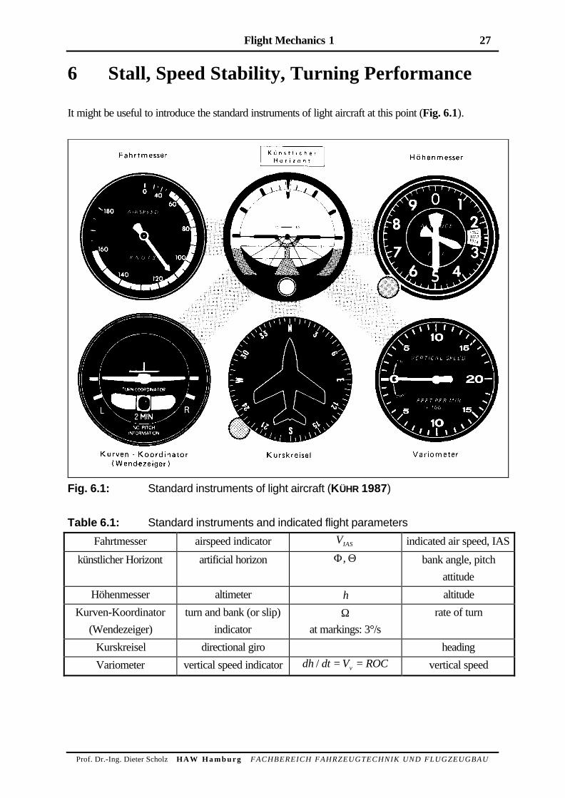
6 Stall, Speed Stability, Turning Performance

It might be useful to introduce the standard instruments of light aircraft at this point (Fig. 6.1).

Fig. 6.1: Standard instruments of light aircraft (KÜHR 1987)

Table 6.1: Standard instruments and indicated flight parameters

Fahrtmesser airspeed indicator VIAS indicated air speed, IAS

künstlicher Horizont artificial horizon Φ Θ, bank angle, pitch

attitude

Höhenmesser altimeter h altitude

Kurven-Koordinator

(Wendezeiger)

turn and bank (or slip)

indicator

Ωat markings: 3°/s

rate of turn

Kurskreisel directional giro heading

Variometer vertical speed indicator dh dt V ROCv/ = = vertical speed



References

ANDERSON 1989 ANDERSON, J.D.: Introduction to Flight. New York : McGraw-Hill,

1989

ANDERSON 1999 ANDERSON, J.D.: Aircraft Performance and Design. Boston : McGraw-

Hill, 1989

GIECK 1981 GIECK, K.: Technische Formelsammlung. Heilbronn : Gieck, 1981

KÜHR 1987 KÜHR, W.: Der Privatflugzeugführer - Technik II. Vol. 3. Bergisch

Gladbach : Schiffmann, 1987

RAYMER 1992 RAYMER, D.P.: Aircraft Design: A Conceptual Approach. AIAA

Education Series, Washington D.C. : AIAA, 1992

LUFTHANSA 1988 LUFTHANSA CONSULTING (Hrsg.): Jet Airplane Performance. 1. Aufl.

Köln : Lufthansa Consulting, 1988



Appendix

A Derivations

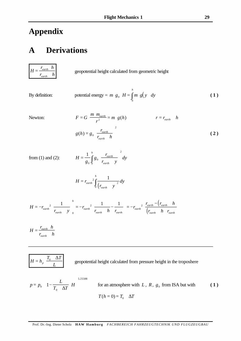
Hr hr h

earth

earth

=⋅+ geopotential height calculated from geometric height

By definition: potential energy = ( )m g H m g y dyh

⋅ ⋅ = ⋅ ⋅∫00

( 1 )

Newton: F Gm m

rm g hearth= ⋅

⋅= ⋅2 ( ) r r hearth= +

g h gr

r hearth

earth

( ) =+

0

2

( 2 )

from (1) and (2): Hg

gr

r ydyearth

earth

h

=+

∫

1

00

2

0

( )H r

r ydyearth

earth

h

=+∫2

2

0

1

( )( )H r

r yr

r h rr

r r hr h rearth

earth

h

earthearth earth

earthearth earth

earth earth

= −+

= −

+−

= −

− ++ ⋅

2

0

2 21 1 1

Hr hr h

earth

earth

=⋅+

H hT T

Lp= ⋅+0 ∆

geopotential height calculated from pressure height in the troposhere

p pL

T TH= ⋅ −

+⋅

0

0

5 25588

1∆

.

for an atmosphere with L , R , g0 from ISA but with ( 1 )

T h T T( )= = +0 0 ∆



p pLT

hp= ⋅ − ⋅

0

0

5 25588

1.

by definition ( 2 )

p pL

T TH p

LT

hp= ⋅ −+

⋅

= ⋅ − ⋅

0

0

5 25588

00

5 25588

1 1∆

. .

from (1) and (2)

1 10

5 25588

0

5 25588

−+

⋅

= − ⋅

LT T

HLT

hp∆

. .

LT T

HLT

hp0 0+

⋅ = ⋅∆

H hT T

Tp= ⋅+0

0

∆

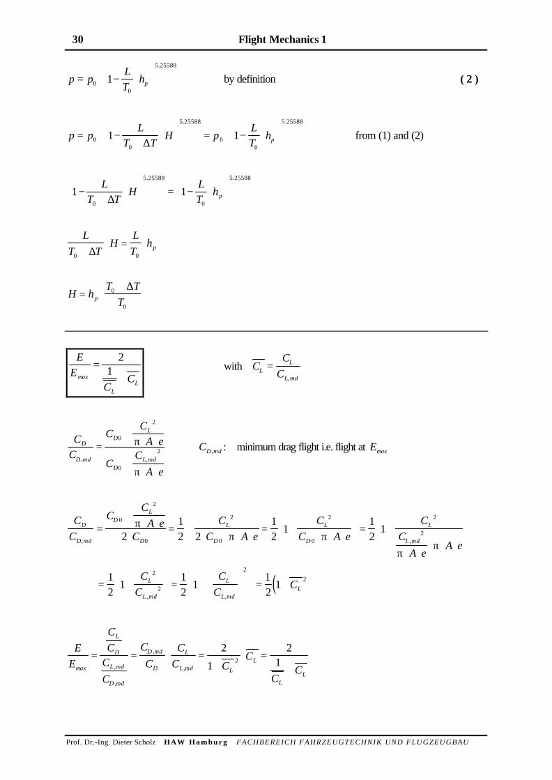
EE

CCmax

LL

=+

21 with C

CCL

L

L md

=,

CC

CC

A e

CC

A e

D

D md

DL

DL md, ,

=+

⋅ ⋅

+⋅ ⋅

0

2

0

2π

π

CD md, : minimum drag flight i.e. flight at Emax

CC

CC

A eC

CC A e

CC A e

CC

A eA e

D

D md

DL

D

L

D

L

D

L

L md, ,

=+

⋅ ⋅⋅

= +⋅ ⋅ ⋅ ⋅

= +⋅ ⋅ ⋅

= +

⋅ ⋅⋅ ⋅ ⋅

0

2

0

2

0

2

0

2

2212 2

12

112

1ππ π

ππ

( )= +

= +

= +

12

112

112

12

2

2

2CC

CC

CL

L md

L

L mdL

, ,

EE

CC

CC

CC

CC C

C

CCmax

L

D

L md

D md

D md

D

L

L md LL

LL

= = ⋅ =+

⋅ =+,

,

,

,

2

1

212



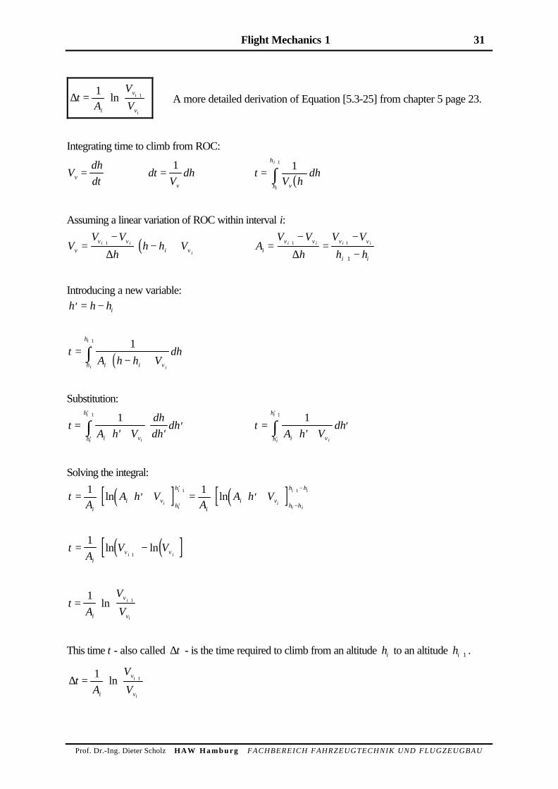
∆tA

VVi

v

v

i

i

= ⋅

+11ln A more detailed derivation of Equation [5.3-25] from chapter 5 page 23.

Integrating time to climb from ROC:

Vdhdtv = dt

Vdh

v

=1

( )tV h

dhvh

h

i

i

=+

∫ 11

Assuming a linear variation of ROC within interval i:

( )VV V

hh h Vv

v vi v

i i

i=

−⋅ − ++1

∆A

V Vh

V Vh hi

v v v v

i i

i i i i=−

=−−

+ +

+

1 1

1∆

Introducing a new variable:

′ = −h h hi

( )tA h h V

dhi i vh

h

ii

i

=⋅ − +

+

∫11

Substitution:

tA h V

dhdh

dhi vh

h

ii

i

=⋅ ′ +

⋅′

′′

′+

∫11

tA h V

dhi vh

h

ii

i

=⋅ ′ +

′′

′+

∫11

Solving the integral:

( )[ ] ( )[ ]tA

A h VA

A h Vi

i vh

h

ii v

h h

h h

ii

i

ii i

i i= ⋅ ⋅ ′ + = ⋅ ⋅ ′ +

′

′

−

−+ +1 11 1

ln ln

( ) ( )[ ]tA

V Vi

v vi i= ⋅ −

+

11

ln ln

tA

V

Vi

v

v

i

i

= ⋅

+11ln

This time t - also called ∆t - is the time required to climb from an altitude hi to an altitude hi+1 .

∆tA

V

Vi

v

v

i

i

= ⋅

+11ln

unterlagen zur vorlesung - haw · pdf filedie vorlesung flugmechanik 1 wird seit ss99...

Documents