unu merit working paper series · unu‐merit working paper series ... skema business school in...
TRANSCRIPT

#2014-012
Technology life cycle and specialization patterns of latecomer countries. The case of the semiconductor industry
Giorgio Triulzi Maastricht Economic and social Research institute on Innovation and Technology (UNU‐MERIT) email: [email protected] | website: http://www.merit.unu.edu Maastricht Graduate School of Governance (MGSoG) email: info‐[email protected] | website: http://mgsog.merit.unu.edu Keizer Karelplein 19, 6211 TC Maastricht, The Netherlands Tel: (31) (43) 388 4400, Fax: (31) (43) 388 4499
UNU‐MERIT Working Paper Series

UNU-MERIT Working Papers
ISSN 1871-9872
Maastricht Economic and social Research Institute on Innovation and Technology, UNU-MERIT
Maastricht Graduate School of Governance
MGSoG
UNU-MERIT Working Papers intend to disseminate preliminary results of research
carried out at UNU-MERIT and MGSoG to stimulate discussion on the issues raised.

1
Technology Life Cycle and Specialization Patterns of Latecomer
Countries. The Case of The Semiconductor Industry*
Giorgio Triulzi
UNU-MERIT and Department of Economics, Maastricht University
This version 24 February 2014
Abstract
Catching-up, leapfrogging and falling behind in terms of output and productivity in high-tech industries crucially depends on firms’ ability to keep pace with technological change. In fast changing industries today’s specialization does not guarantee tomorrow’s success as changes in the technological trajectories reward and punish firms’ specialization patterns. This highlights the importance of studying the relationship between technology life cycle and specialization patterns of new and incumbent innovators. From an empirical point of view life cycles have been extensively analysed at the industry and product level but not so deeply at the technology one (even though plenty of theoretical contributions exist). We define a methodology to describe the life cycle stages of the main technological paradigm within an industry and of the technological areas it is composed of. The methodology is based on the analysis of the age composition of the different areas and of the characteristics of their technological trajectories. We use the classification of the life cycle stages of the single areas to investigate specialization patterns of new and incumbent innovators. Our results show that up to the end of the 1990s firms from Taiwan, Korea and Singapore specialized mainly in areas at the later stages of their life cycles, whereas US and Japanese firms were comparatively better in younger areas. Specialization patterns changed in the beginning of the 2000s, when the Asian Tigers started to become comparatively stronger in emerging areas.
Keywords: Technology Life Cycle, Industry Life Cycle, Product Life Cycle, Specialization Patterns, Technological Paradigms, Technological Trajectories, Main Path Analysis, Catching-up, Semiconductors, Citation networks, Community Detection.
JEL classification: O20, O32, O33, O38
* The author would like to thank Bart Verspagen, Bronwyn Hall, Roberto Fontana, François Lafond, Önder Nomaler and participants to the 8th European Meeting on Applied Evolutionary Economics (EMAEE 2013) at SKEMA Business School in Nice for useful comments and suggestions. Any remaining errors are mine.

2
1. Introduction
The striking example of sustained fast economic growth and huge structural transformation that several
countries like the Asian Tigers (Hong Kong, Taiwan, South Korea and Singapore) and BRICS (Brazil,
Russia, India, China and South Africa) have provided in the last half-century, have been explained by a
variety of points of view. A now widely accepted explanation points to the role of technology as engine
of economic growth and source of competitiveness. Several authors argued that the development of
internal technological skills and the access to foreign technology is the key factor behind the process of
catching-up (Fagerberg and Godinho, 2005; Hobday, 2000; Perez and Soete 1988; Verspagen, 1991;
Abramovitz, 1994). Other authors (e.g. Perez, 1988 and Lee and Lim, 2001, Lee et al. 2005) specified
that the process of catching-up might be better described in some cases as leapfrogging, arguing that
“the latecomer does not simply follow the path of technological development of the advanced countries. They perhaps skip
some stages or even create their own individual path, which is different from the forerunners” (Lee and Lim, 2001,
p.460). Of course technology is in continuous evolution and therefore, as explained by Dosi (1982),
technological change creates and destroys capabilities, thus creating more or less entry, catching-up and
leapfrogging opportunities. Product and industry life cycles have been extensively analysed since the
seminal work of Vernon (1966). However, despite the variety of contributions coming from different
disciplines, like Industrial Organization, International Economics, Innovation Studies and Management
(see, for instance, Klepper, 1996; Malerba and Orsenigo, 1997; Camerani and Malerba, 2007; Boschma
and Frenken, 2011, Bergek et al., 2013, Karniouchina et al., 2013), if we look at this literature from the
perspective of technological catching-up, conflicting predictions on the relationship between product
life cycle and the entrance of new players in the industry arise. According to the international product
life cycle theory latecomer innovators are more likely to specialize in obsolete technologies, whereas
industry life cycle theory (Klepper, 1996, 1997) predicts higher entrance to occur in the earlier stages of
the life cycle. This paper contributes to shed light on the relationship between technology life cycle and
specialization patterns of new innovators. The semiconductor industry provides a particularly suitable
ground for testing such relationship. Indeed, given its peculiarities, a persistently evolving knowledge
base, interacting technological trajectories, short business cycles and increasing global competition
(Brown and Linden, 2009), today’s specialization is no guarantee of tomorrow’s success. Therefore it is
crucial to understand in which areas of the semiconductor technology and at which stage of their life
cycle new entrants specialize. This is the motivation behind this paper. For this purpose we develop a
methodology to define and analyse the life cycle of the semiconductor technologies. First we identify a
set of the most influential patents from the point of view of the development of the main technological
trajectories, using the main path approach developed originally by Hummon and Doreian (1989) and
3
subsequently refined and applied in recent works by Verspagen (2007), Fontana et al., (2009), Martinelli
(2008; 2009), Bekkers and Martinelli (2010). This set of patents is used to define the semiconductors
main technological paradigm. Within this set we identify several interrelated technological areas using a
community detection method proposed by Newman (2004). Then we develop a methodology to
describe the life cycle stages of these areas according to their age and the characteristics of their
technological trajectories. This second methodology is the core and main source of novelty of this
paper. This methodology will be used to answer two research questions: (i) In which technological area new
innovators specialize? (ii) Are there significant differences in the specialization patterns of new innovators from different
countries?
We use data from the second version of the NBER patent citation database (Hall et al., 2001). The
NBER database provides data about patent citations from patent applications and patents issued by the
USPTO from 1976 to 2006. Since US are a crucial market for semiconductors we assume that any
technologically relevant invention in this field is patented at the USPTO. We split the analysis into six
periods (1976-1980, 1981-1985, 1986-1990, 1991-1995, 1996-2000, 2001-2006), in order to analyse the
evolution of the life cycle of a set of technological areas and to investigate whether firms’ specialization
changes accordingly.
This paper is divided as follows. First we briefly review the main theories of latecomers’ specialization
patterns that can be found in the literature (Section 2). Then we present an overview on the technology
and industrial dynamics of the global semiconductor industry (Section 3). In Section 4 we describe the
methodology used to identify the set of key technologies within the semiconductor industry and analyse
their life cycle. Finally we present the results which answer the two research questions (§ 5).
2. Life cycle theories and latecomers’ specialization patterns
The first prominent model which explicitly discussed the relationship between the development stage
of an industry and entry of firms from developing countries was Vernon’s product life cycle (Vernon,
1966). Vernon argues that countries’ comparative advantage might reverse during the product life cycle
and, in the maturity and saturating phase, developing countries which formerly had a comparative
disadvantage in the given technology might start to specialize in it. Vernon’s idea is that follower
countries can take advantage of the fact that fixed initial investments and R&D costs had been
sustained by incumbents and can therefore produce the given product more cheaply. Furthermore, as
the technology becomes mature, leading firms start looking for other possible markets. This opens up
entry opportunities for follower firms. Vernon’s hypothesis, which is widely accepted in the

4
international economic literature (e.g. Grossman and Helpman, 1991 and 2005; Lu, 2007; Borota, 2012;
Ederington and McCalman, 2012), would therefore predicts that entrance from emerging countries
occurs in mature or declining technologies. Vernon’s theory has raised some criticisms which focused
mostly on the fact that today’s production is characterized by fragmented value chains and modular
technologies and can therefore happen in more places simultaneously. Furthermore the leapfrogging
argument has also been used to object Vernon’s conclusions. Product life cycle theory was then lately
refined by numerous authors from numerous disciplines, perhaps the most famous contribution by
Utterback and Abernathy (1975). Klepper (1997), whose extensive work focused on looking for
industry regularities in the course of the life cycle (see also, Klepper, 1996) summarizes the main
conclusions of the product life cycle (PLC) theory as follows: “While distinguishing stages is somewhat
arbitrary, the essence of the PLC is that initially the market grows rapidly, many firms enter, and product innovation is
fundamental, and then as the industry evolves output growth slows, entry declines, the number of producers undergoes a
shakeout, product innovation becomes less significant, and process innovation rises.” (Klepper, 1997, p.149). Therefore,
modern industry life cycle theory predicts, sustained by strong empirical evidence, that the number of
new entrants should be larger in the earliest stages of the industry. This comes from the technological
regime that characterize early stages of the life cycle, as argued by Breschi et al. (2000) which state that
“ceteris paribus high technological opportunities tend to favour the technological entry of new innovators” (Breschi et al.,
2000, p.393). Finally, the work by Christensen (1997), suggests a different mechanism of entrance. The
author defines a particular category of technologies which he calls disruptive. Disruptive technologies
have the peculiarity to be initially less performing than established ones but to eventually over take
them after they start to diffuse. In their early stage, disruptive technologies are more likely to address
smaller markets than established technologies. Thus they are more likely to be developed by new
entrants as incumbent firms have little to gain from introducing them. Christensen’s definition of
disruptive technologies was later generalized to all cases in which incumbents simply fail to foresee the
new technological opportunities or, due to path dependency, get locked in technologies that eventually
will become obsolete. Even though they do not explicitly distinguish between entrance from leader and
follower countries, modern PLC theory’s and Christensen’s conclusions seem to be more consistent
with the leapfrogging hypothesis that firms from latecomer countries do not necessarily have to follow
the predefined technological trajectory but, to the contrary, can set a new one by specializing in
growing areas. The conflicting predictions about which stage of the life cycle should attract most of the
entrance from latecomers raises the need to shed more lights on the relationship between entrance of
emerging players and stage of the technology life cycle, in order to improve our understanding of
catching-up.
5
3. Technology and Industrial Dynamics of the Global Semiconductor
Industry
We focus our study on the semiconductor industry. Semiconductors are the best example of a high-
tech industry in which catching-up, and possibly leapfrogging, by former laggard countries like Taiwan,
Korea, Singapore and China, prominently occurred. The rise of these countries as global players can be
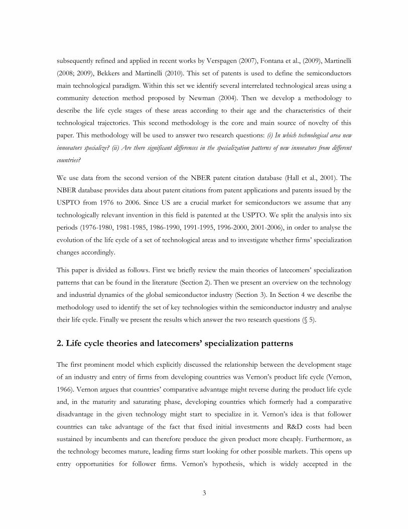
analysed from different point of views. Figure 1 (taken from Brown and Linden, 2009) shows the main
challenges that the semiconductor industry faced between the 1980s and the 2000s. These are the rising
costs of fabrication and design, the reduction in margins due to fall in consumer prices, the
approaching physical limits to miniaturization as indicated by the Moore’s Law1 and the increasing
global competition. These challenges are strongly interconnected and show how technological change
affects the economic development of the industry and the rise of global competition and vice versa. In
this study we do not analyse the economic side of the industry in isolation. We rather focus precisely on
the relationship between the evolution of semiconductor technologies and the economics of catching
up. The direction of technological change ultimately “rewards” and “punishes” specialization strategies
of firms and countries, thereby affecting firms’ entry, survival and success.
Figure 1: The interdependence between technology, economics and global competition
(Source: Brown and Linden, 2009)
For instance, from the beginning of the 1980s onwards the modularization of the semiconductor
manufacturing technology fragmented the value chain fostering specialization. New firms could now
1 In 1965, Gordon Moore, co-founder of Intel Corporation noted that the number of components on an integrated circuits had doubled every year from the invention of the integrated circuit in 1958 until 1965 and predicted that the trend would continue (Moore, 1965). Moore’s law helped guiding the industry’s innovative efforts, setting a defined technological trajectory based on a constant rate of miniaturization of the components of an integrated circuit (Epicoco, 2013).

6
enter the industry at different stages of the production process. As argued by Adams et al. (2013), “the
increased adoption of Complementary Metal Oxide Semiconductor (CMOS) production processes weakened the
interdependence of product design and manufacturing. [...] With the creation of standardized interfaces between
components and Electronic Design Automation (EDA) tools a modular system developed. [...] The interdependence
between product design and manufacturing was weakened in many product segments in semiconductors and specialist firms
were able to enter the industry at both the design and the manufacturing stages” (Adams et al., 2013, p.287).
Furthermore, on the product side the development of Application Specific Integrated Circuits (ASICs)
and of systems on a chip (SoC), which squeezed all components of an electronic system into a single
chip, also allowed the creation of more customized applications, fragmenting the market and creating
entry and survival opportunities for small firms (Fontana and Malerba, 2010; Ernst, 2005; Linden and
Somaya, 2003). Moreover, further miniaturization was also made possible by technological
advancements in lithography, allowing exploring new innovative solutions. This shows how changes in
technology strongly affect industrial dynamics. In the following we look at a few indicators which
describe the evolution of the industry in terms of business cycles, entrance, concentration and
innovation prospects.
Figure 2 shows the cumulated revenues for the largest semiconductor companies. There are three main
types of players in the industry, Integrated Device Manufacturers (IDM), which design, manufacture
and commercialize their own chips, fabless companies, which specialize in the design of semiconductor
devices and foundries, which manufacture them on behalf of third parties2. We distinguish between the
cumulated revenues of the largest ten IDM and fabless and the largest ten foundries in the world in
order to show how lower the revenues of the latter are compared to the former.
2 Other noticeable players are equipment and material suppliers and research providers (governmental or non-governmental research organizations and universities). Due to either the lack of data about their revenues or the lack of profit-orientation we do not take them into consideration in Figure 2.

7
Figure 2: Cumulated revenues for the largest semiconductor companies in the period 1987 -
2011 (Source: author’s elaboration based on ICinsights annual reports)
Figure 2 clearly shows the cyclical trend of the semiconductor industry. Periods of sustained revenues
growth are constantly followed by periods of decline. This is also explained in ICE (1996):
“[In the] long term, the sustained profitability of the semiconductor manufacturers depends on each company's ability to maintain high enough profit margins on the devices it produces to allow sufficient capital outlays for future generations of devices. From year to year, the health of the semiconductor industry as a whole is indicated by its characteristic "boom" and "bust" periods, known as the silicon cycle. Since 1978, there have been four growth cycles in which sales grew an average of 30 percent per year. Following each growth cycle, the industry experiences a one to two year period when sales growth averaged slightly under 4 percent.” (ICE, 1996)
Furthermore, the growth trend shows that starting from the mid-1990s the length of these cycles
considerably reduced. The cyclicality of the semiconductor industry at the business level provides a
strong reason for studying its life cycle at the technological level.
Another interesting characteristic of the industry is the high competition, which maintained the
cumulative share of revenues for the largest four companies (i.e. the C4 index) stable around 30 per
cent over time, as shown in Figure 3. The relative low concentration can be explained by the fact that
the semiconductor industry is made by several different markets, with different demand characteristics
(Brown and Linden, 2009 and Fontana and Malerba, 2010). Therefore several technological areas co-
exist within the industry, providing a second argument to analyse their life cycle.

8
Figure 3: Share of cumulative revenues for the largest four companies – C4 (Source: author’s calculation based on Figure 2)
From the technological point of view there are a set of indicators that hint to the fact that the industry
faced a phase of technological shakeout in the first half of the 2000s. This is something that will be
argued more clearly in the rest of the paper but we can already infer it from the evolution of the relative
number of patents in each of the technological classes to which single patents are assigned. The
changes in the number of new innovators, incumbent innovators and the trend toward technological
concentration, further confirms it. These indicators are shown in the two panels of Figure 4.
Figure 4: Industry technological evolution over time
(a) Percentage of patents per
USPTO technological classes: 438–
process, 257-product, 326-materials,
505-programmability, 716-design
(b) Number of new
innovators, incumbents
and the Herfindal-
Hirshman index
0%
5%
10%
15%
20%
25%
30%
35%
40%
19
97
19
98
19
99
20
00
20
01
20
02
20
03
20
04
20
05
20
06
20
07
20
08
20
09
20
10
20
11
C4
Co
nce
ntr
ati
on
in
de
x

9
It is important to note that the percentage of patents by technological class shown in panel (a) is not
calculated based on all patents granted by the USPTO and classified in one of the semiconductor
subclasses (i.e. 438–process, 257-product, 326-materials, 505-programmability, 716-design). Rather, we
refer to the percentage by class with respect to a subset of technologically influential patent identified
through the main path approach, which we will introduce in Section 4.1. The same holds for panel (b),
where by new innovators we refer to firms that hold at least one patent in the subset of technologically
influent ones for the first time and by incumbent innovators we mean firms that had at least one patent
in that subset in the period(s) before. Note that the use of the terms “new innovators” or “incumbent
innovators” rather than new entrants or simply incumbents is purposely made. Industrial organization
theory would distinguish between firms that have started producing semiconductor devices for the first time
(new entrants) or have been doing it for a while (incumbents). To the contrary we look at the
technological dimension rather than the manufacturing one. Accordingly we characterize firms by their
ability to generate technological inventions that have been lately diffused through a sequence of
improvements (i.e. a technological trajectory). Therefore we argue that simply holding a number of
patents do not necessarily make a firm an innovator. Through our technological trajectory-oriented
framework we are able to distinguish innovations from inventions by identifying which patents are
included in the subset of technologically influent patents and which ones are not. In this sense we use
the term innovation in a Schumpeterian way, implying that inventions became innovations only when
they are recognized as useful and therefore start diffusing. Panel (a) of Figure 4 shows that up to the
beginning of the 1980s product and process innovation were equally important in terms of their relative
size then, for the rest of the period, the latter progressively offset the former. We also see that material
technology lost importance from the 1990s onwards in favour of innovations more related to the
programmability of semiconductor devices. If we interpret these results from the point of view of
industry life cycles the increasing importance of process-oriented over product-oriented innovation
suggests the emergence of a dominant design and the entrance of the industry in the maturity phase
(see, for instance Utterback and Abernathy 1975). This would be usually associated with a decreasing
number of new entrants (new innovators in our case) and an increasing concentration index. Panel (b)
shows somehow contradictory evidences of that. The trend of innovative entrance appears to be quite
cyclical, with two peaks reached in the second half of the 1980s and the 1990s. The number of
incumbents, on the other hand, increases constantly (although at a decreasing pace) up to the end of
the 1990s. This clearly points to the fact that some of the new innovators managed to successfully
establish themselves in the industry, thereby increasing the number of incumbents over time (although,
quite expectedly, by less than the amount that would have been reached if all previous incumbents and

10
new innovators would have survived from one period to the next one). It is worth noticing that
something interesting happened in the first half of the 2000s. Both the number of new innovators and
incumbents decreased strongly. Consequently the concentration index (we use the well-known
Herfindal-Hirshman Index –HHI) explodes in the beginning of the 2000s, pointing to an increased
concentration of the share of technologically influential patents in the hands of a few firms. Therefore,
at the technological level, the semiconductor industry is undergoing what is commonly defined as a
shakeout in the 2000s. This provides an additional motivation to analyse the life cycle of the industry at
the technology level. Lastly, given the focus of this paper, it is interesting to analyse the trend of new
innovators of Figure 4b at the country level. Figure 5 shows the share of new innovators by
geographical origin.
Figure 5: New entrant innovators by country of origin
As we can see innovative entrance is in accordance with our knowledge of the evolution of the global
semiconductor industry. The share of US new innovators decreased over time up to the end of the
1990s, in favour of a larger entrance in the technological area by firms from Taiwan, Korea and
Singapore, which account for about 20 per cent of all new innovators in the 1990s. To the contrary the
share of new innovators from Japan is rather constant across our sample. Finally it is interesting to note
that, despite European firms becoming quite marginal players in the global semiconductor industry,
they seem to be able to still play a significant role at the technological level, at least in terms of
innovative entrance.

11
4. Methodology and Preliminary Analysis
We develop a methodology to classify technological areas according to their life cycle stage. This
methodology consists of a two-steps cluster analysis which combines community detection techniques
for citation networks (the first step, explained in §4.2) with a method to describe communities
according to their node composition (the second step, introduced in §4.3). We apply this methodology
to the subset of patents that characterize the evolution of the semiconductor technology. This subset is
identified using the network of main paths approach. The way this subset is constructed is crucial to
understand the logic behind the classification of the technology life cycle. Hence, in the following, we
first introduce the network of main paths methodology and afterwards we describe the two-step cluster
analysis technique.
4.1 The network of main paths
The network of main paths (NMPs) is a methodology developed to identify the routes through which
knowledge diffuses in large citation networks (made of patents or publications). When applied to patent
citation networks this methodology allows to analyse the evolution of the main sequences of
technological improvements in a given industry or technological area. The first building block of this
approach relates to the meaning of patent citations. If patents B cites patent A then the former
improves upon the latter. In other words A represents the state-of-the-art concerning the particular
technology described in patent B at the moment in which patent application B was filed. Therefore
citations can be interpreted as a measure of technological relatedness3 and provide insights on the
direction of technological change. Of course a patent can cite and be cited by many patents, hence, if
we want to follow the main trajectories of technology evolution among a set of patents, we first need to
decide which direction to take at every junction. This is what the NMPs does. First we calculate the
weight of every citation using the search path node pair (SPNP) algorithm, as developed by Batagelj
(2003). The SPNP returns the number of times that each citation link lies on all possible paths
connecting any node to anyone else. This is easily calculated by multiplying the number of patents that
reach (through direct and indirect citations) the cited patent by the number of patents that are reached
(directly or indirectly) by the citing patent. Therefore a high SPNP weight indicates that the given
3 From this perspective the well known fact that many, if not most, of the citation are added by the patent examiner rather than the applicant plays in our favor. Indeed patent applications are examined by expert in the field of the technology described by the patent. Therefore citations added by examiners can be seen as an even more objective measure of technological relatedness among patents. Obviously the examiner’s citations are instead much more of a problem if one wants to use them as a measure of spillover between patent assignees. Fortunately this is not the case in this work.

12
citation and the two patents involved are located in a highly connected and connecting area of the
network, meaning that the given citation has a strong technological influence, as many paths of
technological improvement pass through it. The NMPs is identified by following the paths emanating
from start nodes (nodes that are cited but not cited), taking at each junction the direction of the citation
which carries the highest weight, till an end point (a node who cites but is not cited) is reached. This
procedure, which had been originally developed by Verspagen (2007) and lately applied by Fontana et al
(2009), Martinelli (2008 and 2009) and Bekkers and Martinelli, (2010), can be better understood with
the help of the example shown in Figure 6.
Figure 6: Identification of the Network of Main Paths
The figure shows a fictitious citation network made of 22 patents. The SPNP weight for every citation
is shown above each line. For instance, the direction of the arrow connecting patents 5 and 9 indicates
that the former is cited by the latter. This citation has a weight of 16, which is given by the
multiplication of the number of patents reaching patent 5, plus 5 itself (i.e. patents 1 and 5), and the
number of patents reached by patent 9, plus 9 itself (i.e. patents 9, 13, 15, 17, 14, 16, 18 and 19). To
identify the NMPs one should start from the set of start nodes (patents 1, 2, 3 and 4) and follow at each
step the citation carrying the highest weight, till one of the end nodes is reached (patents 17, 18, 191 21
and 22). For instance if we start from patent 1, we should proceed to patent 5 and 9, then we should
take patent 14 at the junction (ignoring patent 13 and those coming after it) and keep going till patents
18 and 19 are reached. By repeating this procedure for each start point we identify the NMPs, which, in
the example above, is made of two components whose nodes are coloured in black (main one) and grey

13
(second one). It is important to notice that the two components of the NMPs are not separated if we
look at the original network, but the white nodes that connect them have a negligible importance from
the point of view of technological trajectories.
This example shows a static perspective on the NMPs. The dynamic approach consists of cumulating
networks at different points in time (e.g. from time t till t+1, then from t till t+2, and so on), such that
we can observe how the entrance of young patents at each point in time affects the presence of old
ones in the network of main paths (i.e. the persistence of old technological trajectories) and the change
in the size of its components. Let’s imagine that a set of 10 new patents would enter in the network
showed in Figure 6, at time t+1. For simplicity let’s imagine that the 10 patents will connect (directly or
indirectly) just to the end points (in reality they could connect to any other patent as well) and, more
precisely, they will connect just to one end point. Three cases might be observed.
CASE 1: If the new entrant patents connect to patent 18 or 19 then the main component in
the NMPs will keep being the largest one and all patents that were previously on the
trajectories within the main component will still be found there. In this case we have stability in
the main technological trajectories. We label this instance of technological change as incremental
cumulativeness. The cumulativeness refers to the fact that new technological solutions builds on
previous one. Hence, skills and knowledge developed in the past are likely to be useful in the
present as well.
CASE 2: New entrant patents connect to either patent 21 or patent 22. If that happens the
sequence of patents 3-7-44-20 becomes the root of the new largest component, which is still
related to the former largest component even though it takes a different technological
trajectory. We refer to this case as an example of discontinuity in the technological trajectory within the
same paradigm. We label this instance of technological change as incremental discontinuity.
CASE 3: Let’s now imagine that the new entrant patents will connect at time t+1 to patent 17.
In this case what was formerly the second largest component becomes the main one. This is
an example of radical change in the technological trajectory. What was previously seen as a secondary
area of research now attracts most firms’ innovative efforts. We label this instance of
technological change as radical discontinuity.
By repeating this analysis for several periods we can assess the evolution of technological trajectories.
This was done in a previous work by the same author (Triulzi, 2013). In this work we want to focus on
identifying which technological areas are touched by the main trajectories and analysing their life cycle.
To do that we group patents within the different components of the NMPs into technological areas.
This is done using a well-known community detection algorithm developed by Newman (2004). We
will explain this community detection procedure in the next subsection but before to do that it is
important to give a brief overview of the network at hands.

14
Before to do that we need to briefly clarify how we interpret the NMPs (an extensive discussion is
reported in Triulzi, 2013). The seminal work by Dosi (1982) theoretically defined technological change
as an interaction between technological paradigms and technological trajectories. Dosi defined the
former as “. . . [a] ‘model’ and a ‘pattern’ of solution of selected technological problems, based on selected principles
derived from natural sciences and on selected material technologies" (Dosi 1982). A technological trajectory is then
defined by Dosi as “. . .the ‘normal’ problem solving activity determined by a paradigm, can be represented by the
movement of multi-dimensional trade-offs among the technological variables which the paradigm defines as relevant. . . "
(Dosi 1982). Within the same paradigm firms can explore different research strategies; therefore several
technological trajectories can co-exist. We argue that the network of main paths, being made of several
components, which in turn includes different technological areas interconnected with each other, can
be interpreted as a representation of the technological paradigm. Consequently the different paths
within the NMPs sketch the main technological trajectories, which might span several technological
areas. Indeed, if we take the semiconductor industry we can say that, for instance, building an integrated
circuit, or a memory device represent the main technological problem which poses several related sub-
problems like its miniaturization, increasing computational power, reducing power consumption,
increasing its customization, reducing the cost of production, cope with design complexity, and so on.
These sub-problems can be detected in the different technological areas which compose the paradigm,
where innovative solutions cluster around selected research questions. Of course the problems to be
solved co-evolve with the paradigm and affect the trajectories of technological improvement. Therefore
single technological areas can become obsolete or undergo major changes which can also affect the
relationship between technological areas. It follows that when several of the areas that are part of the
main component of the NMPs becomes mature or start exhausting their attractiveness, the vital force
of the main trajectory begins to reduce, setting the stage for a new one (i.e. what we described under
case 3 above).
Table 1 reports some basic statistics about the NMPs for the periods considered. Figures showing the
main component of the NMPs for the six periods are reported in the Appendix A.1. The technological
areas it is consists of, are highlighted in different colours (these areas have been identified through the
community detection procedure explained in Section 4.2). Looking at Table 1 the reader will notice that
the main component of the NMPs for the periods 1976-1995 and 1976-2006 decreased in size
compared to the periods before them. This can be explained applying the framework discussed above.

15
Table 1: Basic network statistics
76-80 76-85 76-90 76-95 76-00 76-06
Whole network - number of patents 2079 5631 12533 26853 54086 114097
Whole network - number of citations 2712 13310 40255 102957 272843 779076
Main component -number of patents 1703 5385 12348 26686 53874 113756
Main component -number of citations 2469 13164 40145 102864 272728 778890
Network of Main Paths - number of patents 1445 3490 6042 10107 15387 23428
Network of Main Paths - number of citations 1403 3291 5697 9489 14588 22077 Network of Main Paths -Main Component – number of patents
694 1540 2678 2043 4557 3544
Network of Main Paths - Main Component – number of citations
756 1597 2734 2064 4617 3562
The drop in the period 1976-1995 was analysed by the same author of this paper in a previous work
(Triulzi, 2013) and explained by the temporary disruption in the technological trajectory which caused
many patents from the main component of the NMPs in 76-95 to move to the second component in
the next period and then brought back into the largest component in 1976-2000. This is an instance of
incremental discontinuity, as previously discussed under Case 2. In the context of this paper it is more
interesting to look at the drop in the last period, when the main component of the NMPs was made of
3544 patents, approximately 1000 patents less than in 1976-2000.
We argue that this second drop in size is a case of radical change in the trajectory (i.e. Case 3 above).
There is an indicator that supports this view. As we explained above a change in the size ranking of the
largest components occurs when new entrant patents connect more to the second component than to
the main one, in a sufficient number to change the hierarchy of the components. Figure 7 shows the
percentage of new entrant patents in the NMPs at each period that attach to the two largest
components.

16
Figure 7
Figure 7 is constructed taking the NMPs for each period and counting the number of young patents
that entered in the whole NMPs at each period considered and the percentage of them which
connected to the first and second largest component. The figure clearly shows that the largest
component of the network of main paths dramatically loses attractiveness over time. To the contrary,
since 1996, the second largest component begins attracting more patents and overtakes the main one
from 2001 onwards4.
Figure 7 clearly shows that, in the last period considered, the main component of the network of main
path is losing importance in favour of the second one. Given that the motivation of this paper is to
analyse the life cycle of the technological areas within the semiconductor industry we decided to include
the second component of the NMPs in the last period into the analysis, to make sure that our
conclusions would not suffer from a myopic focus on the largest component only. In the next two
sections we will explain how we identify technological areas within the NMPs and how we classify the
stage of their life cycle
4 It is interesting to report that the abstracts of the patents belonging to emerging areas of the second largest component in the 2000s, reveal a focus on touch screens and energy-saving technological solutions. This suggests that the second largest component of the NMPs is composed of technological areas more related to portable devices (like smart phones and tablets) than to desktop computers and laptops. This would confirm the interpretation of a radical change in trajectory because the technical requirements of those devices are quite different from the technological problems posed by the manufacturing process of PCs and laptops.

17
4.2 Grouping patents into technological areas
Figure 6 shows a small fictitious network; one can imagine large-scale networks to be much more
complex, as those shown in Appendix A.1. Hence it became common practice to analyse their
community structure in order to split them into partitions. Partitional and agglomerative hierarchical
clustering methods have been defined to identify such structure. We use a method proposed by
Newman (2004) based on the concept of modularity, which is defined as follows:
Where eii is the fraction of edges falling within community i and ai2 is equal to the squared sum of edges
falling between communities, as . Newman (2004) explains that modularity Q can be also
calculated as the fraction of edges that fall within communities, minus the expected value of the same
quantity if edges fall at random without regard for the community structure. The author highlights that
if a particular division gives no more within-community edges than would be expected by random
chance modularity Q would be equal to zero. This approach allows to optimize modularity Q without
the need to try all possible partition combinations (which would take an amount of time exponential to
the number of nodes in the network). The optimization approach starts from the worse possible
combination and then start an iterative aggregation process which stops when the increase of
modularity becomes negative. Obviously, as explained by Newman (2004), since the joining of a pair of
communities between which there are no edges at all can never result in an increase in Q, one needs
only consider those pairs between which there are edges. Then the change in Q upon joining two
communities is given by:
We chose to use the Newman algorithm because, contrary to other popular community detection
algorithm like, for instance, the Newman and Girvan one (2003), the former provides a benchmark to
evaluate the quality of the partition and does not require to arbitrarily choose the number of
communities to be identified. Indeed the modularity maximization procedure and the comparison with
equivalent random networks returns the best partition of the network analysed, without assuming a pre-
existing community structure.
The application of the Newman algorithm to the network of main paths calculated for the periods of
observation returns the modularity values shown in Figure 8.

18
Figure 8: Modularity of the network of main paths
The high values of modularity (always higher than 0.85) reveal a strong underlying community structure
within the largest component (and the second one in the last period) of the NMPs, providing support
for looking at the different technological areas within the Semiconductor technology separately.
Table 2 shows some basic statistics about the technological areas of the semiconductor technology. As
we can see the algorithm identifies a number of areas varying between 14 and 15 over the periods
observed. The size of the largest area changes quite a lot and so does the standard deviation and the
coefficient of variation.
Table 2: Basic statistics for the technological areas identified by the Newman algorithm
76-80
76-85 76-90 76-95 76-00 76-06 (1st Comp.)
76-06 (2nd Comp.)
Number of patents 694 1540 2678 2043 4557 3544 2762
Number of clusters 14 15 14 14 15 15 14
Size of the main cluster 128 328 368 272 637 701 489
% of patents in main cluster 18,44% 21,30% 13,74% 13,31% 13,98% 19,78% 17,70%
Size of smallest cluster 15 29 52 65 62 73 53
% of patents in smallest cluster 2,16% 1,88% 1,94% 3,18% 1,36% 2,06% 1,92%
Average cluster size 49,57 102,66 191,29 145,93 303,80 236,27 197,29
St.dev. 34,16 80,38 80,41 69,76 143,03 149,51 118,04
Coefficient of variation (St.dev/Av) 0,69 0,78 0,42 0,48 0,47 0,63 0,60
0.82
0.83
0.84
0.85
0.86
0.87
0.88
0.89
0.90
0.91
0.92
1976-1980 1976-1985 1976-1990 1976-1995 1976-2000 1976-2006
1st component 2nd component

19
The large difference in size among technological areas within the same technological paradigm is a
second hint of the importance of analysing the technological areas life cycle. In the next subsection we
explain how we characterize the life cycle.
4.3 Characterizing technological areas according to their life cycle stage
The starting point to define the life cycle of technological areas is to acknowledge that firms’ innovative
efforts cluster around a set of solutions to specific technological problems. The centrality of these
problems and the relevance of the solutions ultimately depend on the evolution of the underlying
technology. Therefore central technological areas today do not necessarily attract the same level of
innovative efforts and interest tomorrow. Even within the same technological paradigm, technological
areas arise, grow, renew and exhaust. During this process of evolution the relationship between
different technological areas might change. This leads to changes in the direction of the technological
trajectories connecting them. As we discuss those changes might be incremental or radical. When most
of the technological areas connected by the main technological trajectory exhaust their innovative
propulsion the entire trajectory suffers from obsolescence and is abandoned in favour of an entire new
set of technological research questions which become the seeds of new technological areas. As we
mentioned earlier, we argue that this is what we observe in the last period considered (2001-2006). This
trajectory-based view on technological change lays at the heart of our methodology to identify the life
cycle of the various semiconductor technologies.
A somehow similar intention can be found in Shibata et al. (2008). However the authors only focused
on emerging areas which they identify by looking at their age. Accordingly, the age of a given
publication or patent is given by the difference between the publication or grant year and the year in
which we are observing the network. The age of a research area is given by the average age of the
publications or patents it is composed of. Shibata et al. define emerging areas as young areas which
have little connections with past research areas (i.e. those observed in the previous time periods of the
network). Figure 9 shows the age of the technological areas that we identified with the Newman
algorithm.

20
Figure 9: Technological areas’ age by period of observation.
The general positive relationship between age and the end year of the period of observation is not
unexpected. After all the longer the period of observation the higher the average age of the
technological areas should be. The interesting fact, however, is that from 1995 we begin to observe
some areas which are much younger than the others. This is much more evident in 2000 and 2006.
These young areas are those that Shibata and colleagues would define as emerging. The authors argue
that there are two types of emerging areas: incremental and branching. According to Shibata et al.
(2008) incremental emerging areas are young areas which are born from a previously existing one,
whereas branching emerging areas are not related to any of the previous research areas5, therefore their
appearance creates a totally new branch of research. The work by Shibata et al. (2008) inspired us to use
a combination of community detection and network analysis methods to identify the stages of the
technology life cycle. We improve upon their work to overcome what we think are two problems with
their approach. First, if we only look at the average age of research areas we cannot identify possible
emerging areas at the beginning of our analysis due to the fact that, by construction, all areas are young
at the beginning of the period of observation. Second with this approach we can identify emerging
areas but we cannot determine the life stage of the older areas. To avoid these shortcomings we
distinguish three types of patents that can be found in the NMPs: young, persistent old and new old. Young
patents are those granted in the last period of observation. Persistent old patents are those that have
5 The use of the term branching by Shibata et al. (2008) is actually a bit confusing given that, by definition, a branch generates from the trunk of a tree.
0
5
10
15
20
25
30
1980 1985 1990 1995 2000 2005
Ag
e o
f th
e t
ech
no
log
ica
l are
a
Period end year
(Circles stand for the technological areas as identified by the community detection technique)

21
already been part of the largest component of the NMPs at least once in the periods before the one
observed. New old patents are patents granted before the last period of observation which were
previously disconnected from the main component of the NMPs. In our analysis we focus on six time
periods: 1976-1980, 1976-1985, 1976-1990, 1976-1995, 1976-2000 and 1976-2006. Let’s take, for
instance, the last period 1976-2006. For this period the three patent categories can be described as
follows. Young patents are those granted after the end of the previous period (i.e. from 2000 till 2006)
which connects to the main component of the NMPs. Persistent old patents are those who showed up
in the main component of the NMPs at least once in one of the previous five periods. New old patents
are those granted before 2001 which had never been part of the main component of the NMPs before.
The distinction between persistent old patents and new old patents allow us to have a deeper look into
old technological areas, distinguishing those which are following a stable technological trajectory (i.e.
incrementally cumulative technological change) from those who are exploring a new one (incrementally
disruptive technological change). Furthermore it also help us to differentiate between areas which are
young but nevertheless building on previously explored technological paths and young areas which are
not related to any technological solution that have been developed in the past. Figure 10 shows the
relationship between the type of old patents and the age of the technological areas. Each circle stands
for one of the technological areas identified over the six time periods. Its position on the horizontal
axis reflects the age of the area. The vertical axis coordinate is given by the percentage of old new and
old persistent patents found in the area (each area accounts for two circles in Figure 10).
Figure 10: The relationship between persistent old patent, new old patents and the age of
technological areas
0%
20%
40%
60%
80%
100%
0 5 10 15 20 25 30
Pe
rce
nta
ge
of
old
pa
ten
ts
Age
Old(new) Old(persistent)
Poly. (Old(new)) Poly. (Old(persistent))

22
The figure shows that young areas are more likely to build on previously unexploited technological
solutions (new old patents) than known ones (persistent old patents). To the contrary, the more a
technological area grows old, the more likely it will follow a stable and previously defined technological
trajectory. This is not surprising, given the cumulative nature of technological change. Figure X clearly
shows that patent composition within a technological area changes drastically with age. This provides
the rationale behind our definition of the technological area life cycle. Our analysis follows the intuition
that it is possible to classify technological areas based on the relative number of young, persistent old
and new old patents, they are composed of. This allows defining all the stages of the life cycle of
technological areas, from emerging to exhausting. Furthermore we break the emerging area category
into two sub-categories, breakthrough areas and disruptive areas, such that we can test Christensen’s
hypothesis that disruptive technologies are more likely to be introduced by new entrants (Christensen,
1997). In the following we describe each stage of the life cycle.
Disruptive emerging areas
It is widely recognized that technological progress has a cumulative nature and today’s solutions are
likely to build on yesterday’s discoveries. This means that even when new technological areas emerge
they might be related to previous technological solutions. Sometimes these solutions might have been
neglected for a while, maybe because their applicability was uncertain at the time of their development,
or because they were initially too costly or just for lack of vision. When they are “re-discovered” and
are subject to new technological improvements they are likely to disrupt the technological trajectory as,
according to the literature, most of the incumbents tend to fail to foresee this kind of technological
change. This is due to myopia of learning (Levinthal and March, 1993) and path dependency, as
explained by Christensen (1997), who defined disruptive technologies in great details. From the point
of view of the network of main paths, we argue that disruptive technological areas are characterized by
the presence of several young patents which builds largely on previously disconnected patents and very
little on persistent old ones.
Breakthrough emerging areas
From time to time the assumption of cumulativeness of technological change is broken and a set of
radical innovations emerge by standing out of the crowd of past technological solutions. Contrary to
disruptive areas breakthroughs are not related to anything developed in the past. From a theoretical
point of view there are three main reasons behind the emergence of breakthroughs. The first one
relates to the entrance of new players, which by definition have less to loose from the introduction of
radical innovations which create discontinuities with respect to skills cumulated in the past. Second,

23
breakthroughs might be developed by companies external to the industry (users or suppliers) on a
necessity-bases or following a vertical integration strategy. These firms tend to bring a different
research perspective which might lead to the appearance of radically new technological solutions. Third,
breakthroughs might emerge in situations when all previous paths have been explored. In this case
necessity brings the courage to experiment totally new solutions. Breakthroughs are obviously rare and
are no guarantee of success. Indeed they might be rapidly abandoned and not developed further if they
fail to establish a new technological trajectory. On the other hand, if successful they strongly shake the
technological paradigm, questioning skills and expertise which have been developed in the past. Given
the way we defined them we argue that breakthrough areas are characterized by a large number of
young patents and a few new old and persistent old patents if at all.
Early growth areas
If successful, disruptive or breakthrough technological areas are developed further and move to a stage
of early growth. During this stage the attractiveness of the area is high and the technological trajectory
starts to consolidate. Therefore the number of young patents is high, the presence of persistent old
patents increases and the one of new old patents decreases.
Mature areas
The following stage is the one of maturity. This stage is similar to the early growth with the only
difference that the area now attracts much less young patents than before and technological change is
even more cumulative, meaning that the number of persistent old patents keeps growing, to the
detriment of the exploration of alternative trajectories.
Renewing areas
After the maturity stage the evolution of a given technological area is at a crossroad. The development
of the given technology could be either stopped or get new vigour. In the former case the technological
area begin exhausting. In the latter it enters into a renewing stage. In this case alternative technological
trajectories are explored to avoid obsolescence. This might begin a new life cycle or just extend a bit the
life of a technological area which will nevertheless exhaust. From the network of main path point of
view renewing areas are characterized by a few young patents which build extensively on new old ones
and on some persistent old patents.
Exhausting areas
There are several reason why a technological area might be abandoned by firms, it could be that it does
not provide interesting technological research questions anymore, or that the underlying technological

24
problems proven to be too challenging (perhaps given the resources and capabilities available at that
point in time) or that the technological trajectory switched to another direction making that particular
area unimportant or just obsolete. No matter what the reason is we argue that exhausting areas are
characterized by very few, if any, young patents, a large number of persistent old patents and almost no
new old ones.
So far we have defined the life cycle stage of a given technological area by arguing that it depends on
how many young, persistent old and new old patents it is composed of. Now we need to define these
quantities more precisely. Quantify how much is a lot is a task that is best done by comparison.
Therefore we first take all areas identified by the Newman algorithm over the periods 1976-19856,
1976-1990, 1976-1995, 1976-2000 and 1976-2006, we look at the percentage of young, persistent old
patents and new old ones in each area and then we plot the distribution of these percentages. This is
shown in Figure 11, where each of the areas is split into three observations indicating the percentage of
young, new old and persistent old patents it is composed of.
Figure 11: Cumulative distribution of the percentage of young, new old and persistent old
patents for all the areas in the periods 1976-1985, 1976-1990, 1976-1995, 1976-2000 and 1976-2006
6 We cannot use the first period, 1976-1980 because, being the initial period, all the areas are entirely composed by young patents.

25
On the horizontal axis we have the values for the percentages of each category of patents that are part
of one of the technological areas, whereas on the vertical axis we have the cumulative percentage of the
distribution, meaning the percentage of observations with a value smaller than the value on the
horizontal axis. We drew two horizontal dashed lines to clearly separate the top 20 percent from the
mid-60 percent and the bottom 20 percent of the distribution. This allows us to identify the border
values for the first quintile and the last quintile. For instance, if we look at the distribution of the
relative number of young new patents among all the technological areas we see that 20 per cent of the
areas have less than 1.14 per cent of young patents, 60 per cent have between 1.14 per cent and 49.35
per cent of them and 20 per cent have more than 49.35 per cent of young patents. This means, for
instance that for an area to have many young patents means to have more than 49.35 per cent of them.
The remaining 50.65 per cent is distributed between new old patents and persistent old ones. The same
exercise can be applied to new old patents and persistent old ones. In the former case 20 per cent of
the areas have less than 11.11 per cent of new old patents, 60 per cent have between 11.11 per cent and
45.57 per cent of them and 20 per cent have more than 45.57 per cent of young patents. Finally, if we
look at the distribution of the relative number of persistent old patents we see that 20 per cent of the
areas have less than 11.97 per cent of them, 60 per cent have between 11.97 per cent and 86.67 per cent
and 20 per cent have more than 86.67 per cent. It is important to notice that there are no areas only
composed by young or new old patents, but there are some which are entirely made of persistent old
patents. This is in line with theoretical expectations based on the intuition that it is easier to follow a
predefined technological trajectory rather than exploring an alternative one. Furthermore from a NMPs
methodological point of view we can argue that an area purely made by young patents or by new old
ones would be disconnected from the main component of the NMPs by construction and therefore not
observed. To the contrary areas entirely composed by persistent old patents can be found in the main
component of the NMPs and serve the purpose of technological ancestors upon which newer areas
build on.
Now that we have more precise numbers which define the quantities of young, new old patents and
persistent old ones, we can use them to elaborate a more precise definition of the life cycle stages of
technological areas.
Table 3 reports the quantile borders for each patent category for each life cycle stage.

26
Table 3: Patent distribution quantile borders by patent type and life cycle stage
Quantile classification
Many Q1 (i.e. top 20%)
Mid Q2, Q3, Q4 (i.e. mid 60%)
Few Q5 (i.e. bottom 20%)
Quantile borders for the technological area life cycle stages
Young patents New old patents Persistent old patents
Breakthrough
emerging areas
Many = Q1 (>49.35%) Few-mid = Q2-Q5
(<45.57%)
Few = Q5 (<11.97%)
Disruptive
emerging areas
Few-mid
= Q2-Q4 (<49.35%)
Many = Q1 (>45.57%) Few = Q5 (<11.97%%)
Early growth
areas
Many = Q1 (>49.35%) Few-mid
= Q2-Q5 (<45.57%)
Mid Q2-Q4
= (11.97%≤ …<86.67%)
Mature areas Few-mid
= Q2-Q4 (<49.35%)
Few-mid
= Q2-Q5 (<45.57%)
Mid Q2-Q4
= (11.97%≤ …<86.67%)
Renewing areas Few-mid
= Q2-Q4 (<49.35%)
Many = Q1 (>45.57%) Mid Q2-Q4
= (11.97%≤ …<86.67%)
Exhausting areas Few = Q5 (<1.14%) Few = Q5 (<11.11%) Many = Q1 (>86.67%)
As the table shows we now have clearer thresholds which define the amount of each type of patents to
be found in a given area for it to be classified in one of the life cycle stage reported in the left column.
We call this thresholds quantile borders. For instance, for an area to be classified as a breakthrough it
needs to have at least 49.35 per cent of young patents, less than 45.57 per cent of new old ones and less
than 11.97 per cent of persistent old patents. However the quantile borders alone are not sufficient to
determine the life cycle stage of each area. The main reason is that, being thresholds, quantile borders
suffer from the drawback that areas which lay very close to the border might actually be more similar to
the areas located on the other side of the border than to the other areas located on the same side. This
problem is similar to the one of defining homogeneous groups of people living in areas whose borders
have been set on paper, without considering the common characteristics of people living close to the
border. In other words we would like to have borders which respect the characteristics of the
technological space and the similarities between the technological areas it is made of. Therefore the
initial quantile borders are used to calculate centroids which will serve as basin of attractions. To sum

27
up, first we calculate the quantile borders for the distribution of the percentage of young, new old and
persistent old patents for all the areas in the periods 1976-1985, 1976-1990, 1976-1995, 1976-2000 and
1976-2006 (Table 3). Then we use them to preliminary identify regions of the technological space that
corresponds to the theoretical description of the technological areas’ life cycle stages. Afterwards we
calculate the centroid for each of the preliminary defined areas. Finally we compute the distance to each
of the centroids for each technological area identified through the Newman algorithm. The life cycle
stage of each technological area is then identified by assigning each area to the closest centroid. This
procedure is shown in Figure 12. Each node stands for one of the technological areas identified in
section 4.2. The size of the node is proportional to the size of the given area in terms of number of
patents. The horizontal axis reports the percentage of persistent old patents, whereas the vertical one
measures the percentage of young patents. Therefore, by construction, none of the technological areas
can lay to the right of the 100 per cent-100 per cent line. Note that the percentages of young, persistent
old and new old patents have to sum up to 100 for each area. This means that the orthogonal distance
from each node to the 100 per cent-100 per cent line is equal to the percentage of new old patents in
the technological area represented by that node. For instance areas on the 90 per cent-90 per cent line
have 10 per cent of new old patents. Hence the percentage of new old patents decreases the further you
get from the origin of the axis. In Figure 12 quantile borders as of Table 4 are drawn in red and
centroids are indicated with a red ‘x’. Nodes of the same colour fall within the basin of attraction of the
same centroid, meaning that they are closer to that centroid than to any other one.
Figure 12: Identification of the centroids of the life cycle stages.

28
Now we have a classification of the life cycle stage of each technological area. To test its logical
consistency we trace movements from each life cycle stage to the other ones. Of course for our
classification to be correct we should observe movements consistent with time. This means that, for
instance patents which are classified into a technological area in its early growth in period T should be
mainly part of a technological area classified as mature in the next period. Some might still be found in
an early-growth area. This would indicate that the life cycle of that area is relatively slow. Some others
might jump over stages and be found in renewing or exhausting areas. This would indicate that the life
cycle of that area moves faster in the period observed. The important thing is that they should not be
found in large numbers in an earlier stage, otherwise the time consistency of our methodology would
be broken. A small number of patents could actually move back to an earlier stage but this can only
happen when some patents from one area serve as foundation for a younger area in the next period.
This possibility is intrinsic to the evolution of communities as defined by the Newman algorithm and
the network of main path approach, but this cannot happen in large numbers because otherwise the
new area would not be younger than the original one and would then be classified in the same life cycle
stage than the latter, or in one of the followings.
Table 4 shows how many patents from areas which, in period T, were in one of the life cycle stages
listed on the rows moved, in the next period, to any of the areas whose life cycle stage in T+1 is
indicated in the columns.
Table 4: Movements from one life cycle stage to the others over consecutive time periods.
The table clearly proves that our methodology is logically consistent as most of the patents follow the
expected movement to “older” life cycle stages (to the right of the diagonal) and very few moves to
“younger” areas whose life cycle stage is antecedent the one of origin (to the left of the diagonal).
Having proved the consistency of our methodology we can now introduce the answer to the paper’s
research questions.

29
5. Results
In the introduction of our paper we raised two research questions: (i) In which technological area new
innovators specialize? (ii) Are there significant differences in the specialization patterns of new innovators from different
countries? In the two following subsections we present the results that answer them.
5.1 New innovators’ specialization pattern
In the first research question of the paper we investigate whether there is a significant difference
between the specialization patterns of incumbent innovators and new innovators. To analyse these
patterns we have to compare in which areas of the NMPs patents belonging to incumbents and new
innovators can be found. Since we want to study specialization patterns at given points in time we will
only look at young patents. If we would include patents granted in the past we would risk getting a
distorted picture of the specialization pattern of incumbent innovators. For instance, a given incumbent
company might have many past patents in a given area but no young ones connected to that area. If we
would not distinguish patent types we would tend to conclude that the given company is specialized in
that area at the time we look at it, when actually this would reflect a past specialization in the area.
In order to analyse specialization patterns we propose an original index which returns a macro picture
of specialization patterns at the country level while taking into account micro specialization patterns at
the firm level. Our specialization index, which we call SPEC, builds on the well-known revealed
technological advantage index (RTA). The RTA is a specialization index defined by Soete (1987), which
builds on the Ricardian concept of comparative advantage and, more precisely on the revealed
comparative advantage index as defined by Balassa (1965). The intuition behind the RTA is that even if
a given entity (countries, firms, geographical regions) in absolute terms might have less patents than
other entities as a whole, there might still be areas in which it enjoys a comparative advantage, meaning
that it is able to produce comparatively more patents in a given technological area than in the whole
industry. Therefore the index reveals the areas of technological specialization, which would possibly
reflect a comparative advantage in terms of research productivity in those areas. The original version of
the index is calculated as follows:
Where xik is entity’s (country or firm) i number of patents in area k. The RTA index is equal to zero
when entity i holds no patents in the given area k. When the index is equal to 1 entity i’s patent share in
area k is equal to its share in all areas. Values of the index greater than 1 indicate specialization in the
given area. The original version of the index is not symmetric, meaning that it is bounded to zero for

30
negative specialization in the area but unbounded for positive specialization, causing problems when
used in econometric models or when one wants to compare its distribution for different entities. For
the sake of our analysis we opt for the symmetric version of the RTA (SRTA), which is calculated as
follows:
In its symmetric version the index ranges from -1 (full negative specialization) to (full
positive specialization), with values greater than 0 indicating positive specialization in the area.
We use the symmetric RTA as a basis to construct an index which gives a micro-founded picture of
specialization patterns at the country level. We first need to estimate the probability density function
(pdf) of the SRTA for each country. The pdf returns the probability to observe a given SRTA value if
we choose a firm at random out of the sample of firms belonging to a given country. We use a kernel
smoothing function to estimate the probability distribution that best fit the empirical (cumulative)
distribution of the SRTA for the given entity. The kernel density function estimates the probability to
observe a given SRTA for the whole range of the SRTA index (from -1 to 1). This improves our ability
to compare entities of different size as the empirical distribution for small entities relies on fewer
observations than for large entities. Once we estimated the probability density function we compute the
SPEC index as follows:
1:1.0:0
)(j
ikjjik SRTASRTASPEC
Our specialization index SPECik is the weighted sum of the probability ρ to observe SRTA values at the
firm level reflecting positive specialization in the given area (i.e. SRTA>0). Indeed ρ(SRTAj)ik is the
probability to observe a given SRTA value j greater than zero (i.e. positive specialization) among the
whole sample of SRTA values calculated for the area k for all firms belonging to the given country i.
This probability is multiplied by the strength of specialization, namely by the value of the SRTA j,
which, ranging from 0 to 1 (we only look at positive specialization), effectively serves as a weight for
the sum. In other words a large value of the SPEC index means that, if we extract a firm at random out
of the sample of firms from the given country, that firm has a high probability to be strongly
specialized in the area under consideration. It is important to note that our index do not make any a
priori assumption about how SRTA values are distributed across firms of the same country. This is an
improvement over traditional approaches which calculated the SRTA at the firm level and then
averaged it at the country level, failing to realize that SRTA might not be normally distributed, making
the average at the country level quite meaningless. Another popular choice is to calculate the SRTA for

31
a given country as the aggregate of all its firms. This approach is also unsatisfactory in the sense that the
aggregate picture might be heavily influenced by a few large firms, wiping out the information about
specialization patterns of small firms. To the best of our knowledge our indicator is the only one that
provides a picture of specialization patterns at the country level which truly respects the underlying
pattern at the firm level. Obviously the same index can be calculated for classes of firms rather than
countries. This is what we do when we compare specialization patterns of new and incumbent
innovators.
Table 5 reports the number of firms by geographic origin and type (new or incumbent innovators)
across the 5 periods under consideration. To answer our two research questions, we merge the first and
second component of the NMPs in the last period together, as explained in Section 4.1.
Table 5: Number of firms by geographic origin and category
All firms 1981-1985 1986-1990 1991-1995 1996-2000 2001-2006 (1st+2nd) Total
US 61 92 62 75 80 370
JP 24 32 28 47 29 160
KR 0 2 5 7 5 19
TW 0 1 6 17 15 39
SG 0 0 1 4 3 8
KR/TW/SG 0 3 12 28 23 66
Total 85 127 102 150 132 596
New Innovators 1981-1985 1986-1990 1991-1995 1996-2000 2001-2006 (1st+2nd) Total
US 35 50 20 40 48 193
JP 13 18 10 25 8 74
KR 2 3 2 3 10
TW 1 5 11 7 24
SG 1 2 1 4
KR/TW/SG 0 3 9 15 11 38
Total 48 71 39 80 67 305
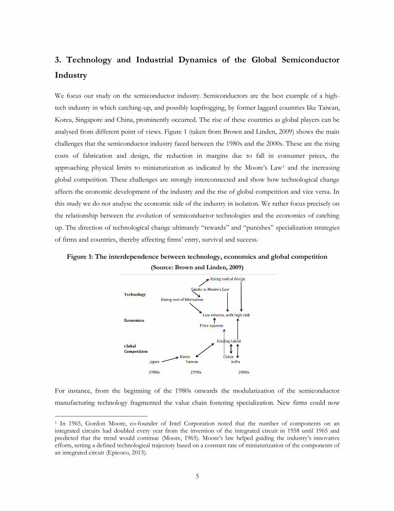
Incumbents 1981-1985 1986-1990 1991-1995 1996-2000 2001-2006 (1st+2nd) Total
US 26 42 42 35 32 177
JP 11 14 18 22 21 86
KR 0 0 2 5 2 9
TW 0 0 1 6 8 15
SG 0 0 0 2 2 4
KR/TW/SG 0 0 3 13 12 28
Total 37 56 63 70 65 291

32
In order to have a reliable estimation for the distribution of SRTAs we will initially plot all periods
together. This gives use 305 observations for the new innovators and 291 for the incumbents. Figure 17
shows the kernel smoothed cumulative distribution functions for the two categories of firms.
Figure 17: Estimated cumulative distribution functions for new and incumbent innovators
The vertical axis reports the probability to observe, across the whole sample, values of the SRTA
smaller or equal than those reported on the horizontal axis. Therefore if one distribution is “smaller”7
7 The correct terms would be first order stochastic dominance if one distribution is always below the other one and second order stochastic dominance if the two distributions cross at some point, meaning that one distribution is below the other only for values greater than a certain threshold. Stochastic dominance refers to the difference in probabilities to observe values of a given amount. If the distribution for one category is stochastically dominated
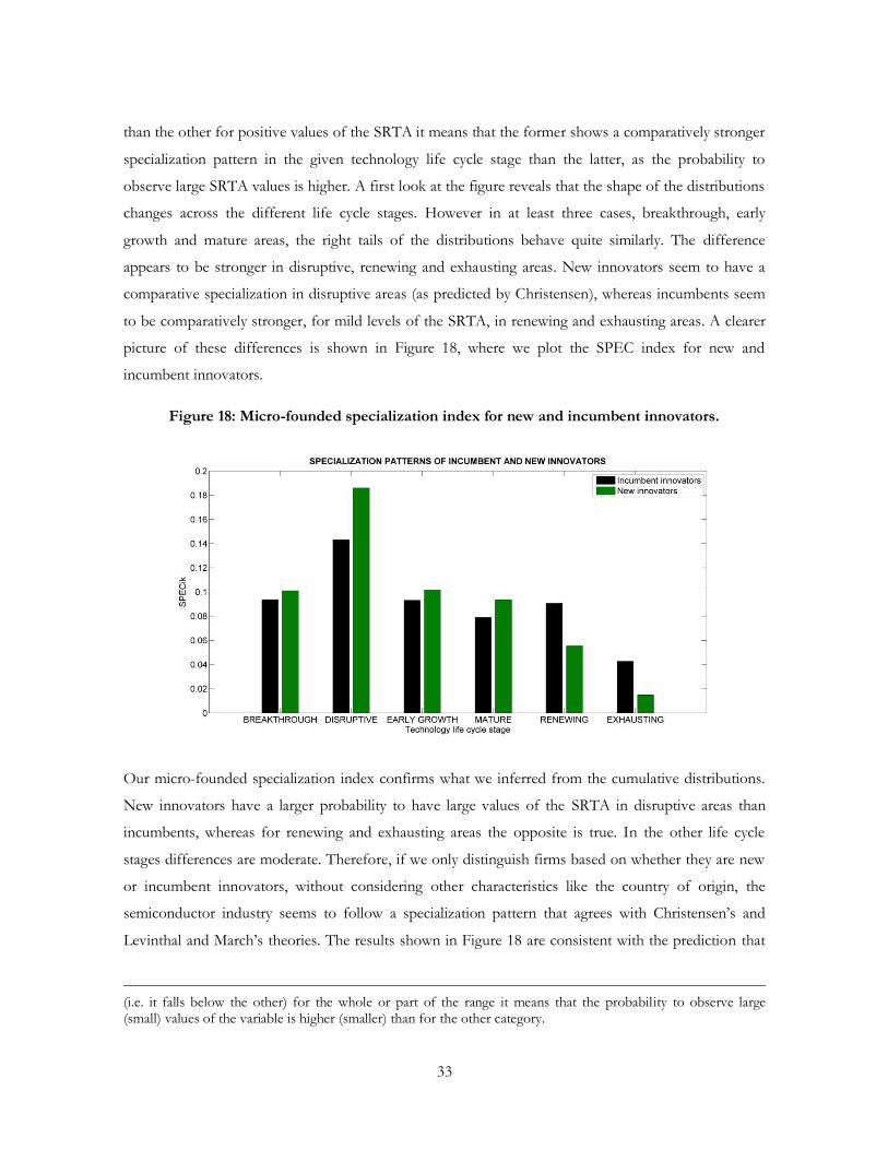
33
than the other for positive values of the SRTA it means that the former shows a comparatively stronger
specialization pattern in the given technology life cycle stage than the latter, as the probability to
observe large SRTA values is higher. A first look at the figure reveals that the shape of the distributions
changes across the different life cycle stages. However in at least three cases, breakthrough, early
growth and mature areas, the right tails of the distributions behave quite similarly. The difference
appears to be stronger in disruptive, renewing and exhausting areas. New innovators seem to have a
comparative specialization in disruptive areas (as predicted by Christensen), whereas incumbents seem
to be comparatively stronger, for mild levels of the SRTA, in renewing and exhausting areas. A clearer
picture of these differences is shown in Figure 18, where we plot the SPEC index for new and
incumbent innovators.
Figure 18: Micro-founded specialization index for new and incumbent innovators.
Our micro-founded specialization index confirms what we inferred from the cumulative distributions.
New innovators have a larger probability to have large values of the SRTA in disruptive areas than
incumbents, whereas for renewing and exhausting areas the opposite is true. In the other life cycle
stages differences are moderate. Therefore, if we only distinguish firms based on whether they are new
or incumbent innovators, without considering other characteristics like the country of origin, the
semiconductor industry seems to follow a specialization pattern that agrees with Christensen’s and
Levinthal and March’s theories. The results shown in Figure 18 are consistent with the prediction that
(i.e. it falls below the other) for the whole or part of the range it means that the probability to observe large (small) values of the variable is higher (smaller) than for the other category.

34
new entrants are more likely to introduce disruptive technologies because incumbents are more likely to
face learning traps that make them over-focusing on their existing capabilities rather than exploring new
ones. To test Vernon’s prediction that new entrants from latecomer countries specialize in areas at the
end of their life cycle we need to further distinguish firms based on their geographical origin. This is
presented in the next section, where we seek an answer for the second research question of the paper.
5.2 Countries’ specialization patterns
In Figure 19 we split new entrant innovators by geographical origin. Once again, in order to have
enough observations for the estimation of the cumulative distribution function we plot all periods
together (this constraint will be removed in the last part of the analysis). Furthermore, for the same
reason, we need to group new innovators from Korea, Taiwan and Singapore into a single geographical
area. For the sake of comparison we plot one additional distribution, which refers to the specialization
pattern of incumbent innovators. This distribution is the same shown in Figure 17.

35
Figure 19: Estimated cumulative distribution functions for new innovators from the US, Japan,
and the three Asian tigers.
The figure reveals insightful differences between the specialization patterns of early entrant (US and
Japan) and latecomer countries (Korea, Taiwan and Singapore). US and Japanese new innovators follow
the same specialization pattern. This is proved by the proximity between the Kernel estimated
cumulative distributions of the SRTA values for US and Japan, in almost all the technology life cycle
stages (with the exception of disruptive areas). To the contrary, there is a remarkable difference

36
between the distributions of the three Asian tigers and those of US and Japan, especially at the
extremes of the technology life cycle. In breakthrough, renewing and exhausting areas, the distribution
of SRTA values for Korean, Taiwanese and Singaporean new innovators is always stochastically
dominated by the distribution for US and Japanese new innovators. This means that Asian tiger’s new
innovators are comparatively more specialized in those areas that US and Japanese ones. The opposite
is true for disruptive areas, whereas there is not much difference for early growth and mature ones.
It is also interesting to compare specialization patterns between new innovators, now split by
geographical origin, and incumbents. In technological areas in the early stages of their life cycle, US and
Japanese new innovators closely follow incumbent innovators’ specialization pattern. On the other
hand, for areas in the late stages (mature, renewing and exhausting), incumbents’ distribution of SRTA
values resembles more to the specialization pattern of new innovators from the three Asian tigers. This
suggests that incumbent strategies are imitated more strongly by US and Japanese new innovators when
it comes to specializing in emerging technologies, whereas they are followed more closely by Asian
tigers’ firms when the decision is about specializing in relatively older technologies.
As done in the previous section, to give a more precise answer to our second research question we look
at the micro-founded specialization index for new innovators by geographical origin. This is reported in
Figure 20.
Figure 20: Micro-founded specialization index for incumbents and new innovators by
geographic origin.

37
Once again the SPEC index confirms the visual impression from the distribution of SRTA values. Let’s
first consider breakthrough, renewing and exhausting areas. If we pick a firm at random out of each of
the samples of new innovators, there is a larger probability that the randomly selected firm has a strong
specialization in those areas if we pick it from the Asian tiger samples rather than the US or Japanese
ones. The opposite is true for disruptive areas, which show a strong specialization by Japanese new
innovators and a clear weakness of the Asian Tigers. For early growth and mature areas it is not easy to
predict the geographic origin of new innovators specialized in them.
What we discussed so far revealed interesting differences between specialization patterns across
geographical areas. However up to now we provided a static analysis, due to the lack of a sufficient
number of observations to have period-by-period reliable estimations for the new innovators. We can
overcome that constraint by looking at all firms together, regardless of whether they are new or
incumbent innovators. This way we are able to show a dynamic picture of micro-founded specialization
patterns at the country level. Figure 21 shows the trend of the SPEC index over time across geographic
areas.
Figure 21: The evolution of the micro-founded specialization index over time.
A dynamic look at specialization patterns reveals that the comparative strength of Asian tigers in
breakthrough areas is recent and started in the 2000s. Up to the end of the 1990s, firms from Korea,

38
Taiwan and Singapore, were comparatively more specialized in renewing and exhausting areas.
Interestingly, an increase of the SPEC index for these firms can also be observed in the 2000s for
disruptive areas. What is also striking is that US and Japanese firms’ comparative technological
advantage in breakthrough areas (and disruptive ones, for Japan only) is decreasing in the 2000s in
favour of areas at later stages of their life cycle (mature, renewing and exhausting).
These results shed light on the different strategies followed by the mayor players of the semiconductor
industry. New entrants from emerging countries successfully catch-up with the leaders by initially
specializing in renewing and exhausting areas. These areas were left free by US and Japanese firms,
which, up to the mid-1990s, were comparatively more specialized in disruptive and early growth areas.
However in the 2000s latecomer countries began to develop a distinct specialization in breakthrough
areas and also an increasing focus on disruptive ones, though maintaining a comparative technological
advantage in exhausting areas. A closer look at the data reveals that the large values of the SPEC index
for Taiwan, Korea and Singapore in breakthrough and disruptive areas in the 2000s, is mainly due to
their specialization in emerging areas belonging to the second component, rather than the first one.
This highlights their ability to anticipate a possible radical change in the trajectory (in favour of portable
devices like smart phones and tablets) and to the effort they devoted to build capabilities in the new
frontier technologies related to touch screen and power saving. Consequently we can conclude that, in
the semiconductor industry, entrance from catching-up countries initially followed the specialization
patterns predicted by Vernon, focusing on renewing old technologies and mastering those that were
getting more obsolete. It then evolved into a specialization more in line with Klepper’s life cycle theory,
in which new entrants focused on younger areas. The latter is also the pattern followed by early entrant
countries, namely US and Japan. Indeed entrance from these countries occurred in younger, and
sometimes disruptive, areas at the beginning of their life cycle, confirming Klepper’s and Christensen’s
theories.
This shows how firms’ strategies matter and ultimately affect specialization patterns at the country level.
Due to space constraint we do not show further details on specialization patterns at the firm level here.
However a series of tables reporting SRTA indexes calculated for the mayor firms in the industry can
be found in the Appendix A.2.
6. Discussion and conclusions
Catching-up and leapfrogging in high-tech industries strongly depends on the direction of technological
change and on the emergence of new technological areas and corresponding decline of old ones. Given

39
the technological and business dynamics discussed in Section 3, namely, short business cycles, high
competition and incremental and radical changes in the technological trajectory, today’s capabilities do
not necessarily ensure long-run survival. This highlights the importance of studying the relationship
between technology life cycle and specialization patterns of new and incumbent innovators. Our study
is one of the few empirical contributions to the discussion of technology life cycles at the artefact level
represented by patents. Patent citation networks offer a fertile ground for such analysis. We provided
new insights on the specialization patterns of semiconductor firms thanks to the combination of three
methodologies: the main path approach, a community detection technique and a cluster analysis based
on the comparison of the trajectories followed by the different technological areas.
First, we highlighted that the analysis of specialization patterns of new innovators and incumbent firms
needs to take the country of origin into consideration, otherwise results might be misleading. Second,
we showed that, until the end of the 1990s, US and Japanese firms were comparatively better in areas at
the beginning of their life cycle, whereas firms from Taiwan, Korea and Singapore, tended to be
specializes in areas which were at later stages of their life cycle, mainly mature, renewing and
exhausting. These specialization patterns changed strongly in the beginning of the 2000s, when firms
from the three Asian tigers started developing a comparative technological advantage in emerging areas,
especially in the second component of the network of main paths, while also keeping being specialized
in exhausting areas. These results are in line with the description of how Korean and Taiwanese firms
managed to build their technological capabilities, as discussed by Chang et al. (1994), Mathews and Cho
(1999), Cho et al. (1998), Chang and Tsai, 2002, Bell and Juma (2008) and Hobday (2000). These
authors agree in highlighting the instrumental role played by Korean and Taiwanese firms’ early
specialization in old foreign licensed technologies to develop internal R&D capabilities lately used to
upgrade their specialization. From the catching-up perspective, the Asian tiger relatively strong position
in emerging areas in the second component of the network of main paths in the 2000s, provides
arguments in favour of the sustainability of their growth path, especially in light of what we describe as
a radical change in the main technological trajectory.
However, it is important to notice that in this work we do not assess the future impact of emerging
areas. Our aim was to analyse whether new entrants specialize in those areas or not. Of course
emerging technologies are intrinsically risky; therefore there is no guarantee that their development will
be sustained in the future. A detailed analysis of how emerging areas affect the future direction of the
technological trajectories goes beyond the scope of this paper. However a preliminary analysis, that was
not reported here, revealed that some areas did generate sustained new trajectories whereas others

40
failed to do so. Since this has crucial implication for catching-up, a full analysis of the knowledge
interaction between the technological areas, and the transferability of capabilities between areas will be
reported in our next work.
Finally we want to praise the strength of using interdisciplinary approaches to disentangle today’s
technological and economic complexity. Several tools have been developed for this purpose, mainly at
the intersection of economics with mathematics and physics. The application of one of them, the
community detection technique, together with a scientometric methodology, the network of main
paths, proved to be extremely insightful to analyse an economic question which occupied scholars at
least since Vernon’s seminal work (1966), namely the one of the relationship between life cycles and
specialization patterns of firms.

41
References
Abramovitz M. (1994), “The Origins of the Postwar Catch-Up and Convergence Boom”, in Fagerberg
J., Verspagen B. and von Tunzelman N. (eds), “The Dynamics of Technology, Trade and Growth”,
Aldershot, UK, Edward Elgar, pp. 21-52.
Adams, P., Fontana, R., Malerba F. (2013), The Magnitude of Innovation by Demand in a Sectoral
System: The Role of Industrial Users in Semiconductors. Research Policy, 42, p.1-14.
Balassa, B. (1965), Trade Liberalization and 'Revealed' Comparative Advantage', The Manchester School of
Economic and Social Studies, Vol. 32, pp. 99-123.
Batagelj V. (2003), “Efficient Algorithms for Citation Network Analysis”, University of Ljubljana,
Department of Mathematics, cs.DL/0309023.
Bekkers R., Martinelli A. (2010), “The interplay between standardization and technological change: A
study on wireless technologies, technological trajectories, and essential patent claims”, Paper presented
at the Druid Summer conference 2010.
Bell Jr, B. W., & Juma, C. (2008). Institutional reform and technology development: the case of ITRI.
International Journal of Technology and Globalisation, 4(3), 296-313.
Bergek, A., Berggren, C., Magnusson, T., & Hobday, M. (2013). Technological discontinuities and the
challenge for incumbent firms: Destruction, disruption or creative accumulation?. Research Policy,
42(6-7), 1210–1224.
Boschma, R., & Frenken, K. (2011). The emerging empirics of evolutionary economic geography.
Journal of Economic Geography, 11(2), 295-307.
Borota, T. (2012). Innovation and imitation in a model of North–South trade. Journal of International
Economics, 87(2), 365-376.
Breschi, S., Malerba, F., & Orsenigo, L. (2000). Technological regimes and Schumpeterian patterns of
innovation. The Economic Journal, 110(463), 388-410.
Brown, C., & Linden, G. (2009). Chips and change: how crisis reshapes the semiconductor industry.
MIT Press, Cambridge, Massachusetts.
Camerani R., & Malerba, F. (2007). Patterns of Technological Entry in Different Fields: an Analysis of
Patent Data. Report to the European Commission. FP6 Project: Knowledge‐Based Entrepreneurship:
Innovation, Networks and Systems.
Chang, P. L., Shih, C., & Hsu, C. W. (1994). The formation process of Taiwan's IC industry—method
of technology transfer. Technovation, 14(3), 161-171.
Chang, P. L., & Tsai, C. T. (2002). Finding the niche position—competition strategy of Taiwan's IC
design industry. Technovation, 22(2), 101-111.

42
Cho, D. S., Kim, D. J., & Rhee, D. K. (1998). Latecomer strategies: evidence from the semiconductor
industry in Japan and Korea. Organization science,9(4), 489-505.
Christensen, C. (1997). The innovator's dilemma: when new technologies cause great firms to fail.
Harvard Business School Press.
Dosi G. (1982), “Technological paradigms and technological trajectories: a suggested interpretation of
the determinants and directions of technical change”, Research Policy, vol. 11, no. 3, June, pp. 147-62.
Ederington, J., & McCalman, P. (2011). Infant industry protection and industrial dynamics. Journal of
International Economics, 84(1), 37-47.
Epicoco, M. (2012). Knowledge patterns and sources of leadership: Mapping the semiconductor
miniaturization trajectory. Research Policy.
Ernst D. (2005), “Internationalization of Innovation: Why is Chip Design Moving to Asia?”,
International Journal of Innovation Management, Vol. 9, No. 1, pp. 47–73.
Fontana R., Nuvolari A., Verspagen B. (2009), “Mapping technological trajectories as patent citation
networks. An application to data communication standards”, Economics of Innovation and New Technology,
Vol. 18 (4), pp. 311-336.
Fagerberg J. and Godinho M. (2005), “Innovation and Catching-up”, in Fagerberg, J., Mowery, D., and
Nelson, R., (eds.), “Oxford Handbook of Innovation”, Oxford Un Press, Oxford, 2004.
Grossman G.M. and Helpman E. (1991), “Quality Ladders and Product Cycles”, The Quarterly Journal of
Economics, Vol. 106, pp.
Grossman, G. M., & Helpman, E. (2005). Outsourcing in a global economy. The Review of Economic
Studies, 72(1), 135-159.
Hall, B. H., A. B. Jaffe, and M. Trajtenberg (2001). "The NBER Patent Citation Data File: Lessons,
Insights and Methodological Tools", NBER Working Paper 8498.
Hall B.H. and Ziedonis R.H. (2001), “The patent paradox revisited: an empirical study of patenting in
the US semiconductor industry, 1979-1995”, RAND Journal of Economics, Vol. 32, No. 1, pp. 101-
128.
Hobday M. (2000), “East versus Southeast Asian innovation systems: Comparing OEM- and TNC- led
growth in electronics”, in L. Kim and R. Nelson (Eds.), “Technology, learning, and innovation:
Experiences of newly industrializing economies”, Cambridge & New York: Cambridge University
Press.
Hummon N.P., Doreian P. (1989). Connectivity in a citation network: The development of DNA
theory. Social Networks, 11, 39-63.
Karniouchina, E. V., Carson, S. J., Short, J. C., & Ketchen, D. J. (2013). Extending the firm vs. industry
debate: Does industry life cycle stage matter?. Strategic Management Journal, 34(8), 1010–1018.

43
Klepper, S. (1996). Entry, exit, growth, and innovation over the product life cycle. The American
economic review, Vol. 86, No. 3, p. 562-583.
Klepper, S. (1997). Industry life cycles. Industrial and corporate change, Vol. 6, No. 1, pp. 145-182.
Fontana, R., & Malerba, F. (2010). Demand as a source of entry and the survival of new semiconductor
firms. Industrial and Corporate Change, 19(5), 1629-1654.
ICE (Integrated Circuit Engineering Corporation) (1996), Status report 1996, National Museum of
American History's Smithsonian Chip Collection, retrieved online on 19/05/2013 at:
http://smithsonianchips.si.edu/ice/cd/CEICM/SECTION1.pdf
Lee, K., & Lim, C. (2001). Technological regimes, catching-up and leapfrogging: findings from the
Korean industries. Research policy, 30(3), 459-483.
Lee, K., Lim, C., & Song, W. (2005). Emerging digital technology as a window of opportunity and
technological leapfrogging: catch-up in digital TV by the Korean firms. International Journal of
Technology Management, 29(1), 40-63.
Levinthal, D. A., & March, J. G. (1993). The myopia of learning. Strategic management journal, 14(S2),
95-112.
Linden, G., & Somaya, D. (2003). System‐on‐a‐chip integration in the semiconductor industry: industry
structure and firm strategies. Industrial and Corporate Change, 12(3), 545-576.
Lu, C. (2007). Moving up or moving out? A unified theory of R&D, FDI, and trade. Journal of
International Economics, 71(2), 324–343.
Malerba, F., & Orsenigo, L. (1997). Technological regimes and sectoral patterns of innovative
activities. Industrial and corporate change, 6(1), 83-118.
Martinelli A. (2008), “Technological Trajectories and Industry Evolution: The case of Telecom
Switching Industry”, Paper presented at the 25th DRUID Summer Conference, Copenhagen.
Martinelli A. (2009), “Market Dynamics and Technological Competences in Ologopolistic Sectors: The
Case of Telecom Switches”, Paper presented at the Druid Summer Conference 2009.
Mathews, J. A., & Cho, D. S. (1999). Combinative capabilities and organizational learning in latecomer
firms: The case of the Korean semiconductor industry. Journal of World Business, 34(2), 139-156.
Newman, M. E. (2004). Fast algorithm for detecting community structure in networks. Physical review
E, 69(6), 066133.
Perez, C. (1988). New technologies and development. In: Freeman, C., Lundvall, B. (Eds.), Small
Countries Facing the Technological Revolution. Pinter Publishers, London.
Perez, C., & Soete, L. (1988). Catching up in technology: entry barriers and windows of opportunity. In:
Dosi, G. et al. (eds) Technical change and economic theory. Pinter, London, pp 458-479.

44
Shibata N., Kajikawa Y., Takeda Y., Matsushima K. (2008). Detecting emerging research fronts based
on topological measures in citation networks of scientific publications. Technovation 28, pp. 758–775.
Soete L. (1987), The impact of technological innovation on international trade patterns: the evidence
reconsidered, Research Policy, Vol.16(2), pp. 101-130.
Triulzi G. (2013). A Path Connectivity Analysis of Technological Change and Industrial Dynamics in
the Semiconductor Industry. Paper presented at the XXXII SUNBELT Conference, Hamburg, 2013.
Utterback, J. M., & Abernathy, W. J. (1975). A dynamic model of process and product innovation.
Omega, 3(6), 639-656.
Vernon R. (1966), “International Investments and International Trade in the Product Cycle”, The
Quarterly Journal of Economics, Vol. 80, No. 2, pp. 190-207.
Verspagen B. (1991), “A New Empirical Approach to Catching Up and Falling Behind”, Structural
Change and Economic Dynamics, Vol. 2, pp. 359-380.
Verspagen B. (2007), “Mapping technological trajectories as patent citation networks: A study on the
history of fuel cell research”, Advances in Complex Systems, Vol. 10 (1), pp. 93-115.

45
Appendix
A.1 Figures of the main component of the network of main paths (NMPs)
1976-1980
1976-1985
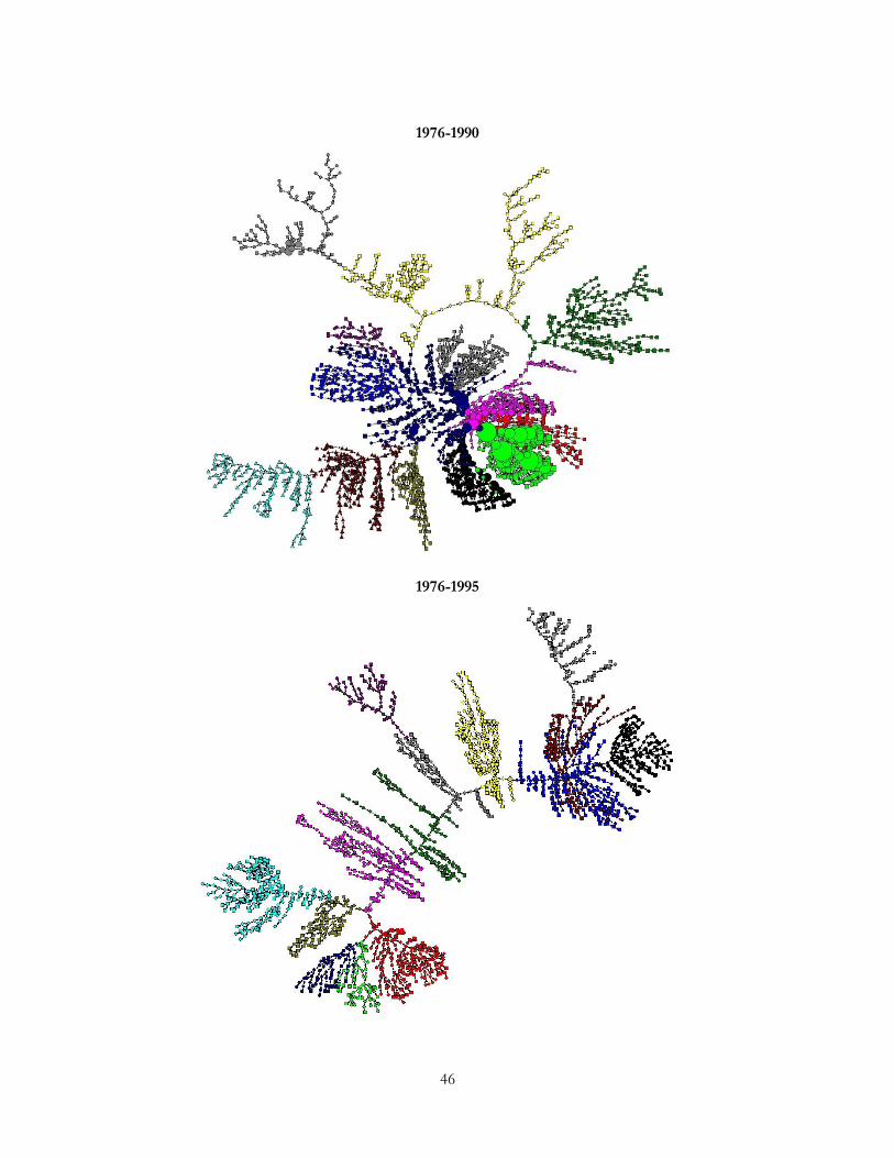
46
1976-1990
1976-1995

47
1976-2000
1976-2006

48
A.2 RTA tables at the firm level
In this section we report the RTA values calculated for a selection of firms from the US, Japan, Korea,
Taiwan and Singapore. To keep the analysis short we do that only for the last three periods. Tables
from A.1 to A.8 reports the RTA values for the main US, Japanese, Taiwanese, Korean and
Singaporean players over time. We highlight values of the RTA greater than 0.2 in bold. Firms are
distinguished between new and inbumbent innovators and also based on their business area
(IDM=Integrated Device Manufacturer, GRO=Government Research Organization, NGRO=Non-
Governmental Research Organization, Equipm.=Equipment supplier). The tables confirm
specialization patterns as discussed in section 5.2. However they provide further details for those
interested to track specialization trends for particular firms or research institutes.
Table A.1: RTA for the top Taiwanese, Korean and Singaporean players (1991-1995)
Company New Inn vs Inc Type #Patents Disruptive Early growth Mature Renewing Exhausting
UMC (TW) New innovator Foundry 31 -0,477 0,230 -0,087 0,597 0,597
SAMSUNG (KR) Incumbent IDM 8 0,046 0,300 -0,365 -1,000 -1,000
TITRI (TW) Incumbent GRO 7 0,112 -0,171 -0,306 0,490 -1,000
HYUNDAI ELEC. (KR) New innovator IDM 7 -0,523 0,359 -0,306 0,708 -1,000
LG ELEC. (KR) New innovator IDM 7 -0,230 -0,171 0,360 -1,000 -1,000
TSMC (TW) New innovator Foundry 6 -0,155 0,245 0,107 -1,000 -1,000
CHARTERED (SG) New innovator Foundry 4 -1,000 0,664 -1,000 -1,000 -1,000
KETRI (KR) Incumbent GRO 3 0,188 -1,000 0,107 -1,000 -1,000
WINBOND (TW) New innovator IDM 2 -1,000 -1,000 0,576 -1,000 -1,000
Table A.2: RTA for the top US and Japanese players (1991-1995)
Company New Inn vs Inc Type #Patents Disruptive Early growth Mature Renewing Exhausting
TEXAS INSTR. (US) Incumbent IDM 39 -0,053 -0,223 0,177 -0,312 0,355
MOTOROLA (US) Incumbent IDM 38 -0,040 -0,211 -0,010 0,235 0,623
MICRON (US) New innovator IDM 38 0,096 0,132 -0,546 0,235 0,037
IBM (US) Incumbent IDM 35 0,159 -0,005 -0,221 -1,000 -1,000
MITSUBISHI (JP) Incumbent IDM 33 -0,073 -0,052 0,189 -0,234 -1,000
TOSHIBA (JP) Incumbent IDM 33 -0,202 -0,538 0,340 0,301 -1,000
NEC (JP) Incumbent IDM 22 -0,335 -0,052 0,375 -1,000 -1,000
AT&T (US) Incumbent IDM 17 0,016 0,186 -0,207 0,093 -1,000
SONY CORP (JP) Incumbent IDM 17 -0,051 -0,264 0,273 -1,000 -1,000
FUJITSU (JP) Incumbent IDM 13 0,083 -0,135 -0,076 0,223 -1,000
HITACHI (JP) Incumbent Equipm. 11 0,089 -0,052 0,007 -1,000 -1,000
NATIONAL SEMICOND. (US) Incumbent IDM 11 -0,002 -1,000 0,340 -1,000 -1,000
HARRIS (US) Incumbent User 7 0,374 -1,000 -1,000 -1,000 -1,000
LSI LOGIC (US) Incumbent Fabless 7 0,305 -0,171 -1,000 -1,000 -1,000

49
APPLIED MATERIALS (US) Incumbent Equipm. 6 0,188 0,245 -1,000 -1,000 -1,000
HUGHES (US) Incumbent User 6 -0,465 -1,000 0,425 0,547 -1,000
MATSUSHITA (JP) Incumbent IDM 6 -0,465 0,245 0,107 -1,000 0,744
OKI ELECTRIC (JP) Incumbent IDM 6 -1,000 0,245 0,425 -1,000 -1,000
SHARP (JP) Incumbent IDM 6 0,046 -0,096 -0,234 0,547 -1,000
SIEMENS (DE) Incumbent IDM 6 0,046 -0,096 0,107 -1,000 -1,000
HONEYWELL (US) Incumbent IDM 5 0,274 -0,005 -1,000 -1,000 -1,000
SEIKO EPSON (JP) Incumbent IDM 5 -0,390 0,597 -1,000 -1,000 -1,000
SEMICOND. ENERGY (JP) Incumbent NGRO 5 -0,065 0,329 -0,147 -1,000 -1,000
Table A.3: RTA for the top Taiwanese, Korean and Singaporean players (1996-2000)
Company New Inn vs Inc Type #Patents Breakthrough Disruptive
Early growth Mature Renewing Exhausting
TSMC (TW) Incumbent Foundry 92 -0,429 -0,310 -0,018 0,004 0,361 -1,000
UMC (TW) Incumbent Foundry 77 -0,725 -0,653 0,089 -0,248 0,101 0,748
SAMSUNG (KR) Incumbent IDM 31 -0,117 -1,000 0,029 0,636 -0,033 -1,000
CHARTERED (SG) Incumbent Foundry 29 -0,224 -0,284 -0,151 0,231 0,385 0,804
VANGUARD (TW) New innovator Foundry 25 -1,000 -1,000 0,160 -1,000 0,075 -1,000
LG ELEC. (KR) Incumbent IDM 21 0,187 -0,130 -0,122 0,377 0,161 -1,000
HYUNDAI ELEC. (KR) Incumbent IDM 17 -0,470 -1,000 0,184 -1,000 -0,402 -1,000
ACER (TW) New innovator IDM 13 -1,000 0,426 0,065 -1,000 0,055 -1,000
TITRI (TW) Incumbent GRO 9 -0,190 -1,000 -0,045 -1,000 0,415 -1,000
MOSEL VITELIC (TW) New innovator IDM 6 0,011 -1,000 -0,098 -1,000 0,415 -1,000
WINBOND (TW) Incumbent IDM 5 0,102 -1,000 -0,007 -1,000 0,184 -1,000
Table A.4: RTA for the top US and Japanese players (1996-2000)
Company New Inn vs Inc Type #Patents Breakthrough Disruptive
Early growth Mature Renewing Exhausting
AMD (US) Incumbent IDM 93 -0,117 -0,704 0,029 0,332 0,111 -1,000
MICRON (US) Incumbent IDM 66 0,011 -0,606 0,068 0,169 -0,205 -1,000
NEC (JP) Incumbent IDM 49 0,239 -0,504 -0,031 -0,027 -0,059 -1,000
IBM (US) Incumbent IDM 37 0,140 -0,392 0,053 0,113 -0,436 -1,000
TEXAS INSTR. (US) Incumbent IDM 36 -0,190 -1,000 0,086 0,126 0,004 -1,000
MOTOROLA (US) Incumbent IDM 35 0,102 -1,000 -0,007 0,598 -0,093 -1,000
TOSHIBA (JP) Incumbent IDM 25 -0,010 -1,000 0,084 -1,000 -0,069 -1,000
MITSUBISHI (JP) Incumbent IDM 21 0,078 -1,000 0,046 -1,000 0,018 -1,000
MATSUSHITA (JP) Incumbent IDM 18 0,463 -1,000 -0,098 0,441 -1,000 -1,000
NATIONAL SEMICOND. (US) Incumbent IDM 17 0,433 -1,000 -0,128 -1,000 -0,079 -1,000
LSI LOGIC (US) Incumbent Fabless 16 -1,000 -1,000 0,244 -1,000 -1,000 -1,000
SHARP (JP) Incumbent IDM 15 0,241 -1,000 -0,007 -1,000 -0,016 -1,000
INTEL (US) Incumbent IDM 12 0,343 -1,000 -0,292 -1,000 0,415 -1,000
LUCENT (US) New innovator User 12 -1,000 -1,000 0,202 -1,000 -0,246 -1,000

50
SONY CORP (JP) Incumbent IDM 11 0,252 -1,000 0,023 0,617 -1,000 -1,000
HITACHI (JP) Incumbent Equipm. 10 -0,240 0,236 0,070 -1,000 -0,159 -1,000
VLSI TECH (US) Incumbent IDM 9 0,154 -1,000 0,046 -1,000 -0,107 -1,000
SEMICOND. ENERGY (JP) Incumbent NGRO 7 -1,000 -1,000 0,244 -1,000 -1,000 -1,000
YAMAHA (JP) Incumbent IDM 7 -0,066 -1,000 -0,031 -1,000 0,349 -1,000
SIEMENS (DE) Incumbent IDM 6 0,508 0,459 -0,570 0,771 -1,000 -1,000
APPLIED MATERIALS (US) Incumbent Equipm. 5 0,421 -1,000 -0,007 -1,000 -1,000 -1,000
UNIV CALIFORNIA (US) Incumbent University 5 -1,000 0,528 -0,007 -1,000 0,184 -1,000
SANYO ELECTRIC (JP) Incumbent IDM 5 0,102 0,732 -0,207 -1,000 -1,000 -1,000
AMERICAN SUPERCOND.(US) New innovator User 5 -1,000 0,883 -1,000 -1,000 -1,000 -1,000
FOVEONICS (US) New innovator User 5 -1,000 -1,000 0,244 -1,000 -1,000 -1,000
Table A.5: RTA for the top Taiwanese, Korean and Singaporean players (2001-2006 – Main
component of the network of main paths)
Company New Inn vs Inc Type #Patents Disruptive Mature Renewing Exhausting
TSMC (TW) Incumbent Foundry 13 0,196 0,397 -0,165 -1,000
SAMSUNG (KR) Incumbent IDM 9 -1,000 0,540 0,095 -1,000
CHARTERED (SG) Incumbent Foundry 4 -0,017 0,580 -0,125 -1,000
UMC (TW) Incumbent Foundry 4 0,318 -1,000 -0,125 -1,000
HYUNDAI ELEC. (KR) Incumbent IDM 3 -1,000 -1,000 0,217 -1,000
VANGUARD (TW) Incumbent Foundry 1 0,589 -1,000 -1,000 -1,000
HYNIX (KR) New innovator IDM 1 -1,000 -1,000 0,217 -1,000
Table A.6: RTA for the top Us and Japanese players (2001-2006 – Main component of the
network of main paths)
Company New Inn vs Inc Type #Patents Disruptive Mature Renewing Exhausting
MICRON (US) Incumbent IDM 75 -0,276 -0,666 0,133 -1,000
AMD (US) Incumbent IDM 31 -0,068 0,489 -0,141 0,509
IBM (US) Incumbent IDM 22 -0,175 0,345 0,029 -1,000
APPLIED MATERIALS (US) Incumbent Equipm. 17 0,494 -1,000 -0,691 0,578
TEXAS INSTR. (US) Incumbent IDM 15 0,015 -1,000 0,065 -1,000
MOTOROLA (US) Incumbent IDM 14 -0,567 0,036 0,142 -1,000
SHARP (JP) Incumbent IDM 11 -1,000 -1,000 -0,005 0,841
INFINEON (DE) Incumbent IDM 4 -0,017 -1,000 0,077 -1,000
NOVELIUS SYSTEMS (US) New innovator Equipm. 4 0,487 -1,000 -0,440 -1,000
LAM (US) Incumbent Equipm. 3 0,589 -1,000 -1,000 -1,000
MATSUSHITA (JP) Incumbent IDM 3 0,126 -1,000 0,018 -1,000
GENUS (US) New innovator Equipm. 3 -1,000 -1,000 0,217 -1,000

51
Table A.7: RTA for the top Taiwanese, Korean and Singaporean players (2001-2006 – Second
component of the network of main paths)
Company New Inn vs Inc Type #Patents Breakthrough Disruptive Mature Renewing Exhausting
TSMC (TW) Incumbent Foundry 40 -0,700 0,100 -0,131 0,000 0,084
SAMSUNG (KR) Incumbent IDM 18 0,594 -0,347 -1,000 -0,091 -1,000
LG PHILIPS (KR) New innovator IDM 13 0,752 -1,000 -1,000 -1,000 -1,000
UMC (TW) Incumbent Foundry 10 -1,000 0,024 -1,000 0,333 -1,000
HYUNDAI ELEC. (KR) Incumbent IDM 9 -1,000 0,152 0,262 -0,286 -1,000
CHARTERED (SG) Incumbent Foundry 7 -1,000 -0,001 0,374 -0,167 0,742
HANN STAR (TW) New innovator IDM 5 0,752 -1,000 -1,000 -1,000 -1,000
KETRI (KR) Incumbent GRO 3 -1,000 0,076 -1,000 0,250 -1,000
MACRONIOX (TW) Incumbent IDM 3 -1,000 0,076 -1,000 0,250 -1,000
CHUNGHWA (TW) New innovator IDM 3 0,752 -1,000 -1,000 -1,000 -1,000
HYNIX (KR) New innovator IDM 3 -1,000 -0,264 0,673 0,250 -1,000
TITRI (TW) Incumbent GRO 2 0,559 -1,000 -1,000 -1,000 0,919
VANGUARD (TW) Incumbent Foundry 2 -1,000 0,272 -1,000 -1,000 -1,000
AU OPTRONIC (TW) New innovator IDM 2 0,752 -1,000 -1,000 -1,000 -1,000
Table A.8: RTA for the top Us and Japanese players (2001-2006 – Second component of the
network of main paths)
Company New Inn vs Inc Type #Patents Breakthrough Disruptive Mature Renewing Exhausting
AMD (US) Incumbent IDM 81 -1,000 0,038 -0,026 0,152 0,401
IBM (US) Incumbent IDM 73 -0,348 0,118 -0,226 -0,187 0,129
TOSHIBA (JP) Incumbent IDM 33 -0,218 0,003 -1,000 0,250 -1,000
TEXAS INSTR. (US) Incumbent IDM 23 -1,000 -0,046 0,335 0,270 -1,000
SEMICOND. ENERGY (JP) Incumbent NGRO 18 0,725 -0,823 -1,000 -0,565 -1,000
MICRON (US) Incumbent IDM 17 -1,000 0,061 -0,050 0,190 -1,000
NEC (JP) Incumbent IDM 13 -0,296 0,193 0,084 -1,000 -1,000
AMBERWAVE SYSTEMS (US) New innovator Equipm. 13 -1,000 0,147 -1,000 0,071 -1,000
INTEL (US) Incumbent IDM 12 -1,000 0,186 -1,000 -0,412 0,595
MITSUBISHI (JP) Incumbent IDM 9 0,404 -0,264 0,547 -0,286 -1,000
SHARP (JP) Incumbent IDM 9 -0,120 -0,675 -1,000 0,591 -1,000
MATSUSHITA (JP) Incumbent IDM 7 -1,000 0,272 -1,000 -1,000 -1,000
FUJITSU (JP) Incumbent IDM 6 0,082 -0,264 0,673 -0,091 -1,000
LSI LOGIC (US) Incumbent Fabless 6 -1,000 0,076 0,673 -1,000 -1,000
MIT (US) Incumbent University 6 -1,000 -0,067 -1,000 0,429 -1,000
CANON (JP) Incumbent User 5 -1,000 0,272 -1,000 -1,000 -1,000
HITACHI (JP) Incumbent Equipm. 5 0,171 0,024 -1,000 0,000 -1,000
HUGHES (US) Incumbent User 5 -1,000 0,272 -1,000 -1,000 -1,000
MOTOROLA (US) Incumbent IDM 5 -1,000 0,024 0,509 -1,000 0,809
FREESCALE (US) New innovator IDM 5 -1,000 0,166 -1,000 0,000 -1,000
INFINEON (DE) Incumbent IDM 4 -1,000 0,134 0,587 -1,000 -1,000
APPLIED MATERIALS (US) Incumbent Equipm. 3 0,650 -0,264 -1,000 -1,000 -1,000
OKI ELECTRIC (JP) Incumbent IDM 3 -1,000 -0,264 -1,000 0,538 -1,000
SONY CORP (JP) Incumbent IDM 3 -1,000 0,076 -1,000 0,250 -1,000

52
AGERE SYSTEM (US) New innovator Fabless 3 -1,000 0,076 -1,000 0,250 -1,000
E INK (US) New innovator IDM 3 0,752 -1,000 -1,000 -1,000 -1,000
HONEYWELL (US) Incumbent User 3 -1,000 0,272 -1,000 -1,000 -1,000
RENESAS ELECTR. (JP) New innovator IDM 3 -1,000 -0,264 0,673 0,250 -1,000

The UNU‐MERIT WORKING Paper Series 2014-01 The medium‐term effect of R&D on firm growth by Marco Capasso, Tania Treibich
and Bart Verspagen 2014-02 Diverse and uneven pathways towards transition to low carbon development: The
case of diffusion of solar PV technology in China Michiko Iizuka 2014-03 User innovators and their influence on innovation activities of firms in Finland by
Jari Kuusisto, Mervi Niemi and Fred Gault 2014-04 Migration, remittances and household welfare in Ethiopia by Lisa Andersson 2014-05 Path‐breaking directions of nanotechnology‐based chemotherapy and molecular
cancer therapy by Mario Coccia and Lili Wang 2014-06 Poor trends ‐ The pace of poverty reduction after the Millennium Development
Agenda Richard Bluhm, Denis de Crombrugghe, Adam Szirmai 2014-07 Firms' adoption of international standards: Evidence from the Ethiopian floriculture
sector by Mulu Gebreeyesu 2014-08 School choice, segregation, and forced school closure by Cheng Boon Ong and
Kristof De Witte 2014-09 Gender difference in support for democracy in Sub‐Saharan Africa: Do social
institutions matter? by Maty Konte 2014-10 Why are women less democratic than men? Evidence from Sub‐Saharan African
countries by Cecilia García‐Peñalosa and Maty Konte 2014-11 Tipping points? Ethnic composition change in Dutch big city neighbourhoods by
Cheng Boon Ong 2014-12 Technology life cycle and specialization patterns of latecomer countries. The case
of the semiconductor industry by Giorgio Triulzi