The Pennsylvania State University

The Graduate School

Department of Astronomy and Astrophysics

UNVEILING THE ACCRETION DISKS THAT FUEL ACTIVE

GALACTIC NUCLEI

A Thesis in

Astronomy and Astrophysics

by

Karen Theresa Lewis

c© 2005 Karen Theresa Lewis

Submitted in Partial Fulfillmentof the Requirements

for the Degree of

Doctor of Philosophy

December 2005

The thesis of Karen Theresa Lewis was read and approved1 by the following:

Michael EracleousAssociate Professor of Astronomy and AstrophysicsThesis AdviserChair of Committee

Steinn SigurdssonAssociate Professor of Astronomy and Astrophysics

W. Niel BrandtProfessor of Astronomy and Astrophysics

Donald SchneiderProfessor of Astronomy and Astrophysics

L. Samuel FinnProfessor of Physics

Lawrence RamseyProfessor of Astronomy and AstrophysicsHead of the Department of Astronomy and Astrophysics

1Signatures on file in the Graduate School.

iii

Abstract

An increasing number of Active Galactic Nuclei (AGN) exhibit broad, double-peaked Balmer emission lines, reminiscent of those observed in Cataclysmic Variables;these double-peaked Balmer lines represent some of the best evidence for the existenceof accretion disks in AGNs. There is considerable evidence to support the hypothesisthat double-peaked emitters are “clean” systems in which the accretion disk is not veiledby a disk wind. This unobscured view affords the opportunity to study the underlyingaccretion disk which is believed to exist in all AGNs. In this thesis, I study two aspects ofdouble-peaked emitters, namely the mechanism responsible for diminishing the accretiondisk wind and the long-term profile variability of the double-peaked emission lines.

It has been argued that double-peaked emitters have accretion flows that transi-tion to a vertically extended, radiatively inefficient accretion flow at small radii. Thisscenario naturally explains the diminished wind in double-peaked emitters, but also of-fers a way to illuminate the outer accretion disk, which is necessary to produce thedouble-peaked emission lines. I critically analyze this hypothesis through robust esti-mates of the accretion rate in a few objects and also through an investigation of theX-ray spectra, which are sensitive to the structure of the inner accretion disk. I findthat this hypothesis may be valid in some, but not all double-peaked emitters. Thus,alternative mechanisms for diminishing the disk wind should be sought; ideally thesemechanisms should also offer a way to illuminate the outer accretion disk. Furthermore,robust estimates of the accretion rate should be determined for a much larger sample ofdouble-peaked emitters in order to determine whether the distribution of accretion ratesis continuous.

A set of 20 double-peaked emitters has been monitored for nearly a decade in orderto observe long-term profile variations in the double-peaked emission lines. Variationsgenerally occur on timescales of years, and are attributed to physical changes in theaccretion disk. The profile variability requires the use of non-axisymmetric accretion diskmodels; a few of the best observed objects have been modeled, with varying degrees ofsuccess, by invoking circular accretion disks with bright spots or spiral arms, or ellipticaldisks. I have characterized the variability of a group of seven double-peaked emitters ina model independent way and found that variability is caused primarily by the presenceof one or more lumps of excess emission that change in amplitude, projected velocity,and shape over periods of several years. An elliptical accretion disk does not producethe correct variability patterns, and for those objects with a known black hole mass, thetimescale for variability in this model is an order of magnitude longer than is observed.The spiral arm model produces variability on the correct timescale, but it is also unableto reproduce the observations. However, I suggest that with the simple modification ofallowing the spiral arm to be clumpy, many of the observed variability patterns couldbe reproduced. To make further progress, it is important to continue monitoring theseobjects at least twice per year. Additionally, a few objects which showed significantvariability should occasionally be monitored intensively (every few weeks) for severalmonths at a time in order to probe variability taking place on the dynamical timescale.

iv

Table of Contents

List of Tables . . . . . . . . . . . . . . . . . . . . . . . . . . . . . . . . . . . . . . vi

List of Figures . . . . . . . . . . . . . . . . . . . . . . . . . . . . . . . . . . . . . vii

Acknowledgments . . . . . . . . . . . . . . . . . . . . . . . . . . . . . . . . . . . viii

Chapter 1. Introduction . . . . . . . . . . . . . . . . . . . . . . . . . . . . . . . . 11.1 The Accretion Disk Paradigm for Active Galactic Nuclei . . . . . . . 11.2 A Brief History of Double-Peaked Emitters . . . . . . . . . . . . . . 3

1.2.1 External Illumination by a Radiatively Inefficient AccretionFlow . . . . . . . . . . . . . . . . . . . . . . . . . . . . . . . . 3

1.2.2 Connection Between Double-peaked Emitters and the GeneralAGN Population . . . . . . . . . . . . . . . . . . . . . . . . . 5

1.2.3 Challenges to the RIAF hypothesis . . . . . . . . . . . . . . . 61.2.4 Variability of the Double-Peaked Balmer Emission Lines . . . 7

1.3 Double-Peaked Emitters — Who Needs Them? . . . . . . . . . . . . 81.4 The Goals of this Thesis . . . . . . . . . . . . . . . . . . . . . . . . . 9

Chapter 2. Black Hole Masses in Double-Peaked Emitters . . . . . . . . . . . . . 112.1 Introduction . . . . . . . . . . . . . . . . . . . . . . . . . . . . . . . . 112.2 Sample Selection, Observations, and Data Reduction . . . . . . . . . 122.3 Analysis and Results . . . . . . . . . . . . . . . . . . . . . . . . . . . 17

2.3.1 Fitting Method . . . . . . . . . . . . . . . . . . . . . . . . . . 172.3.2 Sources of Systematic Error . . . . . . . . . . . . . . . . . . . 172.3.3 Notes on Individual Objects . . . . . . . . . . . . . . . . . . . 18

2.4 Discussion and Conclusions . . . . . . . . . . . . . . . . . . . . . . . 19

Chapter 3. XMM and RXTE Observation of 3C 111 . . . . . . . . . . . . . . . . 233.1 Introduction . . . . . . . . . . . . . . . . . . . . . . . . . . . . . . . . 233.2 Properties of 3C 111 . . . . . . . . . . . . . . . . . . . . . . . . . . . 253.3 Observations and Data Reductions . . . . . . . . . . . . . . . . . . . 27

3.3.1 XMM-Newton . . . . . . . . . . . . . . . . . . . . . . . . . . . 273.3.2 Rossi X-ray Timing Explorer . . . . . . . . . . . . . . . . . . 29

3.4 Timing Analysis . . . . . . . . . . . . . . . . . . . . . . . . . . . . . 303.5 Spectral Analysis . . . . . . . . . . . . . . . . . . . . . . . . . . . . . 30

3.5.1 Continuum Models . . . . . . . . . . . . . . . . . . . . . . . . 323.5.2 Models for the Fe KαLine . . . . . . . . . . . . . . . . . . . . 373.5.3 Combined Continuum and Fe KαEmission Models . . . . . . 42

3.5.3.1 Truncated Accretion Disk - Models #7a,b . . . . . . 423.5.3.2 Highly Ionized Accretion Disk - Models #8a,b,c . . 433.5.3.3 Partial Covering - Model #9 . . . . . . . . . . . . . 46

v

3.6 Discussion . . . . . . . . . . . . . . . . . . . . . . . . . . . . . . . . . 493.6.1 Origin of the Low Energy Component . . . . . . . . . . . . . 493.6.2 Interpretation of the Spectral Models . . . . . . . . . . . . . . 50

3.7 Conclusions . . . . . . . . . . . . . . . . . . . . . . . . . . . . . . . . 52

Chapter 4. Long-Term Profile Variability in Double-Peaked Emitters . . . . . . 544.1 Introduction . . . . . . . . . . . . . . . . . . . . . . . . . . . . . . . . 544.2 Observations and Data Reductions . . . . . . . . . . . . . . . . . . . 574.3 Profile Anlysis . . . . . . . . . . . . . . . . . . . . . . . . . . . . . . . 61

4.3.1 Relative Narrow and Broad Line Fluxes . . . . . . . . . . . . 644.3.2 Difference Spectra . . . . . . . . . . . . . . . . . . . . . . . . 674.3.3 Variations in Profile Parameters . . . . . . . . . . . . . . . . 754.3.4 Variations with Integrated Broad Hα Flux . . . . . . . . . . . 79

4.4 Model Profile Characterization . . . . . . . . . . . . . . . . . . . . . 814.4.1 Physical Motivation . . . . . . . . . . . . . . . . . . . . . . . 814.4.2 Calculation of the Model Profiles . . . . . . . . . . . . . . . . 834.4.3 Model Characterization . . . . . . . . . . . . . . . . . . . . . 84

4.5 Discussion and Interpretations . . . . . . . . . . . . . . . . . . . . . . 894.6 Conclusions . . . . . . . . . . . . . . . . . . . . . . . . . . . . . . . . 91

Chapter 5. Conclusions and Suggestions for Future Work . . . . . . . . . . . . . 935.1 Viability of the RIAF scenario . . . . . . . . . . . . . . . . . . . . . . 935.2 Characterization of the Long-term Profile variability . . . . . . . . . 945.3 Accretion Disk Winds in Double-Peaked Emitters . . . . . . . . . . . 95

Appendix A. Telluric Correction Method . . . . . . . . . . . . . . . . . . . . . . 96

Appendix B. Inclination Angle of the Disk in 3C 111 . . . . . . . . . . . . . . . 99

Appendix C. Total Galactic Hydrogen Column Density Towards 3C 111 . . . . . 100

Bibliography . . . . . . . . . . . . . . . . . . . . . . . . . . . . . . . . . . . . . . 101

vi

List of Tables

2.1 Galaxy Properties . . . . . . . . . . . . . . . . . . . . . . . . . . . . . . 132.2 Template Stars . . . . . . . . . . . . . . . . . . . . . . . . . . . . . . . . 132.3 Velocity Dispersions and Derived Properties . . . . . . . . . . . . . . . . 21

3.1 Observation Log . . . . . . . . . . . . . . . . . . . . . . . . . . . . . . . 283.2 Best Fit Continuum Parameters . . . . . . . . . . . . . . . . . . . . . . . 333.3 Best Fit Parameters for Combined Continuum and Fe KαLine Models . 47

4.1 Galaxy Properties . . . . . . . . . . . . . . . . . . . . . . . . . . . . . . 564.2 Instrumental Configurations . . . . . . . . . . . . . . . . . . . . . . . . . 584.3 Log of Observations . . . . . . . . . . . . . . . . . . . . . . . . . . . . . 59

vii

List of Figures

2.1 Observed Ca ii lines and Best-fit Models . . . . . . . . . . . . . . . . . . 16

3.1 3C 111 X-ray Lightcurve . . . . . . . . . . . . . . . . . . . . . . . . . . . 313.2 X-ray Spectra of 3C 111 . . . . . . . . . . . . . . . . . . . . . . . . . . . 343.3 Confidence Contours in the Column Density and Photon Index . . . . . 353.4 Confidence Contour in the Folding Energy and Reflection Fraction . . . 363.5 Confidence Contours for Gaussian Fits to the Fe KαLine . . . . . . . . 393.6 Confidence Contours for the Disk-line Fits to the Fe KαLine (Powerlaw

+ soft Gaussian Continuum) . . . . . . . . . . . . . . . . . . . . . . . . 403.7 Confidence Contours for the Disk-line Fits to the Fe KαLine (Powerlaw

+ Compton reflection continuum) . . . . . . . . . . . . . . . . . . . . . . 413.8 Ratio of the REFSCH and Power Law Models . . . . . . . . . . . . . . . 443.9 Confidence Contour in the Ionization Parameter and Reflection Fraction 453.10 Confidence Contour in the Column Density and Covering Fraction for

the Partial Covering Model . . . . . . . . . . . . . . . . . . . . . . . . . 493.11 Confidence Contours for the Gaussian Fit to the Fe KαLine (Partial

Covering Model) . . . . . . . . . . . . . . . . . . . . . . . . . . . . . . . 53

4.1 Double-Peaked Balmer Emission Line Profile . . . . . . . . . . . . . . . 614.2 Broad Hα Light Curves . . . . . . . . . . . . . . . . . . . . . . . . . . . 664.3 Difference Spectra . . . . . . . . . . . . . . . . . . . . . . . . . . . . . . 684.4 Variations in Profile Properties as a Function of Time . . . . . . . . . . 774.5 Variations in Peak Separation with Broad Hα Flux . . . . . . . . . . . . 804.6 Model Profiles . . . . . . . . . . . . . . . . . . . . . . . . . . . . . . . . . 85

A.1 Un-corrected Spectrum of IRAS 0236.6–3101 . . . . . . . . . . . . . . . 96A.2 Example Fit of a Rapidly Rotating B-star and the Residuals . . . . . . 98

viii

Acknowledgments

I am first and foremost grateful to my parents, my first teachers, and all of myfamily for their moral support during my twenty-three years in school! Secondly, I amindebted to my advisor Mike Eracleous for his willing advice and assistance, in mattersboth large and small, and also his (seemingly) endless reserves of patience. Finally Iwould like to thank the Penn State Astronomy Department for providing such a wonder-ful group of people to work (and relax) with. Numerous members of the department havehelped me during the last six years and I cannot possibly give credit to everybody, butI would especially thank Tamara Bogdnovic, John Debes, Jie Ding, Julian van Eyken,Suvrath Mahadevan, Mike Sipior, and Michele Stark for helping me to keep the loss ofsanity to a minimum, especially during the “early years”.

I would like to thank my thesis committee for their useful advice and suggestions.Chapter 3 of this thesis was previously published (ApJ, 622, 2, 618); I would like toacknowledge the work of Mario Gliozzi who prepared the Rossi X-ray Timing Explorerdata for analysis and also performed the timing analysis. I also gratefully acknowledgethe work of Rita Sambruna and Richard Mushotzky who provided valuable scientificinput. The code I used to perform the relativistic blurring in Chapter 3 was generouslyprovided by Andy Fabian. There are numerous individuals with whom I’ve had engagingscientific conversations during the course of working on this thesis, including but certainlynot limited to Mateo Guinazzi, Aaron Barth, Jonathon Gelbord, David Ballantyne, SuviGezari, and John Everett.

The results on the long-term variability of the double-peaked Balmer lines inAGNs would not have been possible without the dedication of many people, in partic-ular Mike Eracleous and Jules Halpern who logged over 100 nights of observing. AlexFilippenko, a dedicated fan of this project, has carried out many observations and pro-vided several spectra. Thaisa Storchi-Bergmann, another dedicated collaborator, hascarried out many observations at CTIO. We also thank Sue Simkin and Bob Becker forproviding specific spectra of Pictor A. Sarah Gallagher, Ann Hornschemeier, and MikeSipior also assisted with some of the observations. Finally I would like to thank the staffat the Kitt Peak National Observatory and the Cerro-Tololo Interamerican Observatoryfor their expertise and helpfulness.

Many of the spectra for the variability study were obtained at the National OpticalAstronomy Observatories and some with the Low Resolution Spectrograph on the HobbyEberly Telescope. The National Optical Astronomy Observatories, which operates theKitt Peak National Observatory and the Cerro-Tololo Interamerican Observatory, is op-erated by AURA, under a cooperative agreement with the National Science Foundation.The Hobby-Eberly Telescope (HET) is a joint project of the University of Texas atAustin, the Pennsylvania State University, Stanford University, Ludwig-Maximilians-Universitat Munchen, and Georg-August-Universitat Gottingen. The HET is namedin honor of its principal benefactors, William P. Hobby and Robert E. Eberly. TheMarcario Low Resolution Spectrograph is named for Mike Marcario of High LonesomeOptics who fabricated several optics for the instrument but died before its completion.

ix

The LRS is a joint project of the Hobby-Eberly Telescope partnership and the Institutode Astronomıa de la Universidad Nacional Autonoma de Mexico.

Finally, I am extremely grateful for the financial support of NASA, throughthe Graduate Student Researchers Program (NGT5-50387) and the Pennsylvania SpaceGrant Consortium Fellowship program. The research presented in Chapter 3 was alsopartially supported by an XMM-Newton grant from NASA (NAG-9982). Additionalsupport for travel to observatories was provided by the Zaccheus Daniel Foundation andthe Association of University for Research in Astronomy, Inc. (AURA).

1

Chapter 1

Introduction

1.1 The Accretion Disk Paradigm for Active Galactic Nuclei

Active Galactic Nuclei (AGNs) are among the most energetic objects in the Uni-

verse, with bolometric luminosities often exceeding 1046 erg s−1. It is now generally ac-cepted that at the heart of these powerhouses lies a supermassive black hole with a massin excess of 106 M that is accreting matter from its host galaxy (see, e.g., Salpeter 1964;Rees 1984; Peterson 1997). As matter spirals inwards, it forms an equatorial accretiondisk around the black hole (such as that described by Shakura & Sunyaev 1973), whoseinner portions are heated to UV-emitting temperatures by “viscous” stresses which tapinto the potential energy of the accreting gas. During the past decade, simulations havemade clear the importance of magneto-hydrodynamical processes in accretion disks, anda more modern theory attributes the “viscosity” to magnetic tension and reconnection.In particular a magneto-rotational instability may play a critical role in allowing the gasin the disk to shed its angular momentum (for a review, see Balbus & Hawley 2003). Theinner accretion flow acts as a central engine, driving many of the observed phenomena.In particular, two of the hallmarks of AGNs—broad emission lines and the emission ofhard X-rays—are directly related to the accretion flow that fuels the AGN, as describedbelow.

The broad emission lines observed in AGNs typically have full widths at halfmaximum (FWHM) of & 5000 km s−1, although some AGNs exhibit lines with FWHM

& 104 km s−1. The widths of these lines are far in excess of the thermal velocity of thegas, which is estimated to be ∼ 10 km s−1 (T ∼ 104 K), and a large bulk velocity of theemitting gas is required to explain them. Furthermore, the broad emission line fluxesrespond to changes in the ionizing continuum on timescales of days to a few light months(e.g. Peterson 1993; Korista 1995; Peterson et al. 2004), indicating that gas in the BroadEmission Line Region (BELR) is located within the inner 0.1 pc of the AGN.

During the past several decades, many observational studies have been under-taken to unravel the nature of the BELR, including large scale surveys, detailed obser-vations of individual objects, and intensive reverberation mapping campaigns, in whichthe response of the broad emission lines to changes in the ionizing continuum flux issystematically monitored. Although a definitive theory of the nature of the BELR re-mains elusive, during the past decade the idea that the BELR is related to the accretionflow that fuels the AGN has been steadily gaining in support in the AGN community,both observationally and theoretically. An historical description of the emergence of thisdisk plus wind scenario for the BELR is beyond the scope of this introduction, but briefreviews are given by Gaskell & Snedden (1999) and Eracleous (2004).

2

The dense accretion disk itself, with densities of 1013−15cm−3, is thought to bea source of the broad, low-ionization Hα, Hβ, and Mg iiλ2798 lines, as first argued byCollin-Souffrin (1987) and Collin-Souffrin & Dumont (1989). This idea is bolstered bythe fact that some AGNs emit double-peaked Hα and Hβ profiles (Eracleous & Halpern1994; Strateva et al. 2003), reminiscent of emission lines from the disks of CataclysmicVariables, where they are an regarded as the kinematic signature of the accretion disk(e.g. Horne & Marsh 1986). These double-peaked emitters are the subject of this thesisand will be described in more detail below and in subsequent chapters.

The accretion disk proper cannot be the sole source of broad emission-lines, how-ever, because it is unable to produce the strong C iii]λ1909, C ivλ1549 and Lyα emissionlines which are commonly observed. The disk is not sufficiently ionized to produce theC iii]λ1909 and C ivλ1549 lines, and the Lyα line photons are effectively trapped inthe dense disk. Furthermore, the majority of AGNs do not emit double-peaked low-ionization emission lines. However, there are several ways in which the disk-signatureof these lines can be masked; I will return to this issue in §1.2.2. Instead, an accretiondisk wind is thought to be an important source of both high- and low-ionization broademission lines as discussed by many authors (e.g., Shields 1977; Emmering, Blandford,& Shlosman 1992; de Kool & Begelman 1995; Chiang & Murray 1996; Elvis 2000). Thiswind is thought to be propelled by a combination of resonant line driving by the UVemission from the inner disk and/or magneto-hydrodynamical forces (e.g. Murray, Chi-ang, Grossman, & Voit 1995; Konigl & Kartje 1994; Proga, Stone, & Kallman 2000;Everett 2004).

The bulk of the line emission is expected to arise in the base of the wind, which isqualitatively similar to an accretion disk atmosphere. In this scenario, the low-ionizationlines form in the densest portions of the wind which sits just above the disk (or in thedisk itself) while the high-ionization lines form in the less dense portions of the windwhich have been slightly accelerated. As clearly demonstrated by Chiang & Murray(1996), although the disk wind is rotating, the lines arising from it are single-peakedbecause the optical depth is not isotropic; photons will escape much more easily alonglines of sight with a low projected velocity, thereby enhancing the core of the profile andsuppressing the wings.

The other ubiquitous feature of AGNs is X-ray emission (e.g. Mushotzky, Done, &Pounds 1993, and also references in Chapter 3), both in the form of continuum emissionwhich extends to hundreds of keV and emission lines, the most prominent being the FeKα fluorescence line at 6.4 keV. The accretion disk around a supermassive black holenever reaches X-ray emitting temperatures, so it is postulated that a corona of energeticelectrons forms in the inner regions of the accretion flow and UV photons from the inneraccretion disk are inverse Compton scattered into the X-ray regime. The exact form ofthis corona (i.e. thermal or non-thermal origin, geometry, etc.) are as yet uncertain, butin all current models, the formation of this corona is intimately related to processes inthe underlying accretion disk (see, e.g., Haardt & Maraschi 1991, 1993; Poutanen 1998,and references therein). Some of these hard photons are scattered and irradiate theunderlying cold, dense disk, leading to several reprocessing features, namely fluorescentemission lines (most notably from Fe Kα ) and continuum emission in the form of a

3

Compton reflection bump, an excess of emission that peaks at ∼ 30 keV. These reflectionfeatures are described in more detail in Chapter 3.

Thus the accretion disk is an integral part of an AGN. Not only does it providea means to feed the supermassive black hole and harness the potential energy of theaccreting matter, but many of the most energetic and ubiquitous features of AGNs areformed in the accretion disk and the associated wind and corona. Although the presenceof an accretion disk in an AGN is now commonly accepted, and in some ways takenfor granted, the direct evidence of this accretion disk is limited. A broad excess of UVemission at wavelengths shorter than ∼ 4000A, known as the “big blue bump”, is thoughtto be the blackbody emission from inner UV emitting portion of the accretion disk (see,e.g., Malkan & Sargent 1982). Additionally, the Fe Kα lines in some AGNs are distortedand their profiles are well-fitted with a model attributing their origin to a disk (see e.g.,Fabian et al. 1995; Nandra et al. 1997, and references in Chapter 3). As mentioned above,some AGNs emit double-peaked Balmer emission lines. These disk-like emission lines,represent the most direct, kinematic evidence for the presence of a large-scale accretiondisk in AGNs. Numerous studies are devoted to the study of Fe Kα emission lines inAGNs, and some of these results are summarized in Chapter 3. The main focus of thisthesis is to study those objects which emit double-peaked Balmer emission lines.

1.2 A Brief History of Double-Peaked Emitters

Double-peaked emission lines were first observed in the broad-line radio galaxies(BLRGs) Arp 102B (Stauffer, Schild, & Keel 1983; Chen & Halpern 1989; Chen, Halpern,& Filippenko 1989), 3C 390.3 (Oke 1987; Perez et al. 1988), and 3C 332 (Halpern 1990).Given the similarity between these lines and those observed in CVs, these authors sug-gested that the lines originated in an accretion disk surrounding the AGN at distancesof hundreds to thousands of gravitational radii (rg = GMBH/c

2, where MBH is themass of the black hole). Later, a survey of BLRGs was undertaken and it was foundthat ∼ 20% of the observed objects exhibited double-peaked Balmer emission lines (Er-acleous & Halpern 1994, 2003). In addition to possessing double-peaked lines, theseobjects have several properties which set them apart from other BLRGs. Their Balmerlines are twice as broad as those found in other BLRGs (the most extreme examples

have FWHM ∼ 40 000 km s−1; Wang et al. 2005), the low-ionization forbidden lines([O i]λ6300 and [S ii]λ6717, 6731) are unusually strong compared to other BLRGs, andthe non-stellar continuum is weaker, with ∼ 50% of the continuum near Hα being at-tributed to starlight from the host galaxy (compared to . 10% for other BLRGs spanninga similar luminosity range.)

1.2.1 External Illumination by a Radiatively Inefficient Accretion Flow

One of the main objections to an accretion-disk origin for the double-peaked (andother) broad emission lines, was that the local dissipative and gravitational energy re-leased by the disk at these large radii (at least in a standard Shakura & Sunyaev thindisk; Shakura & Sunyaev 1973) was insufficient to power the observed lines (Shields 1977;Chen et al. 1989). Thus Chen & Halpern (1989) postulated that the outer accretion disk

4

was illuminated by a vertically extended structure in the inner accretion disk, such asthose found in the two-temperature disk solutions described by Shapiro, Lightman, &Eardley (1976) and Rees et al. (1982). These and other radiatively inefficient accretionflows (RIAFs), such as Advection Dominated Accretion Flows (ADAF; Narayan & Yi1994, 1995) or Convection Dominated Accretion Flow (CDAF; Quataert & Gruzinov2000; Narayan, Igumenshchev, & Abramowicz 2000), are thought to form when the ac-

cretion rate is very low, relative to the Eddington accretion rate,1 because the coolingtimescale due to collisions between the electrons and ions is greatly increased; in par-ticular the ions become extremely hot (T∼ 109–1011 K). In the outer disk, the gas cancool effectively and the disk remains geometrically thin and optically thick. At someradius, the accretion disk becomes dominated by gas pressure (due to the inability ofthe ions to cool), causing the disk to become geometrically thick and optically thin. Inote that when the accretion rate is very high, relative to the Eddington accretion rate,a vertically extended structure (a radiation supported torus, Rees et al. 1982) can alsoform. This flow is still optically thick and only slightly hotter than the standard thindisk, but is radiatively inefficient because the accretion timescale is shorter than thecooling timescale.

The illumination of a dense accretion disk by a weak source of high-energy pho-tons, such as that produced by a RIAF, was investigated by Collin-Souffrin (1987) anda subsequent series of papers (Collin-Souffrin & Dumont 1989, 1990; Dumont & Collin-Souffrin 1990a,b,c). These authors found that the heating of the disk by the externalillumination accounted for the “missing” energy and that the physical conditions in theheated gas were in agreement with those required by photoionization models to reproducethe observed low-ionization lines.

There is considerable support for the hypothesis, at least among the well-studiedobjects in the Eracleous & Halpern (1994) sample, that the inner accretion flow indouble-peaked emitters has the form of a RIAF instead of a standard geometrically thinaccretion disk. The Spectral Energy Distributions (SEDs) of Arp 102B and 3C 390.3lack the “big blue bump”. This deficit of UV emission is also observed in Low IonizationNuclear Emission Line Regions (LINERs; Heckman 1980) as shown, for example, by Ho(1999) and those LINERs that are powered by accretion onto black hole are generallyconsidered to harbor a RIAF.

Furthermore, the unique properties of the double-peaked emitters in the Eracleous& Halpern (1994) sample, namely strong low-ionization lines and relatively weak non-stellar continuum (which would arise in the inner disk), suggest indirectly a deficit ofUV emission in double-peaked emitters in general. Nagao et al. (2002) performed pho-toionization calculations and showed that the observed [O i]/[O iii] and [O i]/[O iii] lineratios are well-reproduced by an SED similar to those observed in LINERs.

1The Eddington luminosity, given by LEdd = 1.38 × 1038M/Merg s−1, is the luminosity atwhich the radiation pressure of the gas will exceed the gravitational force of the accreting object.The Eddington accretion rate is given by mEdd = LEdd/η c

2, where η is the efficiency with whichgravitational energy is converted into radiation. The transition to a two-temperature flow occurswhen m/mEdd . α2, where α is the Shakura-Sunyaev viscosity parameter (Rees et al. 1982).The ratio of the bolometric luminosity to LEdd is commonly used as a proxy for m/mEdd; whenLBol/LEdd < ηα2 ∼ 10−3, the inner accretion flow might take the form of a RIAF.

5

These similarities to LINERs are underscored by the discovery of double-peakedemission lines in several LINERs, including NGC 1097 (Storchi-Bergmann, Baldwin, &Wilson 1993), M81 (Bower et al. 1996), NGC 4203 (Shields et al. 2000), NGC 4450 (Hoet al. 2000), and NGC 4579 (Barth et al. 2001). Given the difficulty of detecting broademission lines in LINERs (Ho et al. 1997b) it is likely that a larger number of LINERsexhibit double-peaked emission lines. A final piece of evidence to support the hypothesisthat the inner accretion flow has the form of a RIAF is provided by the UV spectra ofdouble-peaked emitters, which are discussed in the next section.

1.2.2 Connection Between Double-peaked Emitters and the General AGN

Population

If all AGNs have accretion disks and double-peaked emission lines arise in thedisk, why don’t all AGNs emit double-peaked emission lines? The UV spectra of double-peaked emitters suggest a possible answer to this question.

An important consequence of a deficit in UV emission is that the accretion-diskwind, which is thought to be partially accelerated by UV resonance line driving, shouldnot be as strong as those observed in AGNs with a big blue bump (Proga et al. 2000).The C iii]λ1909, C ivλ1549 and Lyα emission lines of Arp 102B are in fact very weak andfurthermore the Mg iiλ2798 line is double-peaked and has a profile that is similar to thoseof Hα and Hβ (Halpern et al. 1996). Six other double-peaked emitters were observedwith the Hubble Space Telescope and a similar phenomenon is observed; preliminaryresults have been discussed by Eracleous (2004). One of the most striking trends is thatas the luminosity of the object increases, the UV resonance lines become more similarto those observed in other AGNs (i.e. stronger and more blueshifted with respect to thenarrow component of the line) and the Mg iiλ2798 line becomes less distinctly double-peaked. A similar luminosity effect is seen in CVs where more luminous systems (i.e.those in outburst) tend to have single-peaked Balmer emission lines as opposed to themore commonly observed double-peaked lines (e.g. Marsh & Horne 1990; Still, Dhillon,& Jones 1995). Murray & Chiang (1996) suggested that this phenomenon is simplydue to the more luminous CVs having a much “stronger” disk wind component in theemission line.

Thus, a reasonable hypothesis is that the accretion disk-wind does not make assignificant a contribution to the broad emission lines in double-peaked emitters as inother AGNs, but that as the luminosity (which should be linked to the accretion rate)increases, the wind begins to make a larger contribution. Certainly the underlyingaccretion disk does not “disappear” as the wind becomes stronger. As demonstratedby Chiang & Murray (1996) and Murray & Chiang (1998), the wind effectively masksthe direct emission from the underlying accretion disk, because the photons emitted bythe disk must pass through the wind and take on a single-peaked velocity profile. Thus,double-peaked emitters may be very similar to other AGNs with the exception that theiraccretion-disk winds are weaker and therefore the double-peaked disk emission lines canactually be observed.

I also note that even in the absence of an accretion-disk wind, there are otherways to mask the signature of the accretion disk. As stressed by Eracleous & Halpern

6

(2003), an emission line from a disk will only appear double-peaked when the ratio ofthe outer to inner radius is small (i.e. an accretion ring, as opposed to a disk). As thisratio increases the two peaks merge together and the resulting profile is similar to thoseseen in many AGNs, particularly when the narrow emission lines are included. Thus itis also possible that the outer boundary of the Balmer line-emitting region of the disk indouble-peaked emitters is unusually small in comparison to other AGNs. However, I notethat this effect alone would not naturally explain the other properties of double-peakedemitters.

1.2.3 Challenges to the RIAF hypothesis

The hypothesis that the inner accretion flows in double-peaked emitters has theform of a RIAF is nicely consistent with the observed properties of the double-peakedemitters in the Eracleous & Halpern (1994) sample and offers a way to link the double-peaked emitters to the general AGN population. However, there is an important chal-lenge to this scenario. Strateva et al. (2003) found over 100 double-peaked emittersin the Sloan Digital Sky Survey (SDSS; York 2000), representing 3% of the z < 0.332AGN population. The properties of the double-peaked profiles in this sample are verysimilar to those of the objects in the Eracleous & Halpern (1994) sample and they ap-pear to originate in the same region of the accretion disk. However, Strateva et al.(2003) found that the general properties of the double-peaked emitters are indistin-guishable from those of the general AGN population, in sharp contrast to the findingsof Eracleous & Halpern (1994). Although the equivalent widths of [O i]λ6300 and the[O i]λ6300/[O iii]λ5007 ratio were larger than in the parent population, there was littledifference in the [S ii]λλ6716, 6731 equivalent width or the [O ii]λ3727/[O iii]λ5007 ratio.In particular, only 12% of the SDSS sample were classified as LINERs by their emissionline ratios.

Taken at face value, these results seem to call into question the hypothesis thatall or even most double-peaked emitters have a RIAF. However, there are few caveats.Firstly, among the Eracleous & Halpern (1994) objects only a handful of objects werestrictly classified as LINERs; most were merely “reminiscent” of LINERs. LINERs arerather extreme objects with LBol/LEdd ∼ 10−6–10−3 (Ho 1999). It is possible that anobject with a slightly larger Eddington ratio could possess a RIAF that transitions toa thin disk at a smaller radius than in LINERs. As a case in point, Gammie, Narayan,& Blandford (1999) performed detailed modeling of the SED in NGC 4258 which hasa well-known black hole mass of (4.0 ± 0.25) × 107M from water maser measurements(Herrnstein et al. 1999). They concluded that the SED was best fitted by a ADAFthat had a mass accretion rate of ∼ 0.01M yr−1, which transitions to a thin disk atr ∼ 10–100rg . The mass accretion rate corresponds to m/mEdd ∼ 0.01, and this objectis classified as a Seyfert 1.9 by Ho, Filippenko, & Sargent (1997a), not as a LINER.This demonstrates that it is possible for non-LINERs and objects with rather high massaccretion rates (compared to LINERs) to possess a small-scale ADAF or other RIAFnevertheless. Furthermore, as pointed out by Chen et al. (1989), if the accretion rate isvery low, the RIAF may extend so far that there is no thin disk to illuminate.

7

I stress that the primary requirements that RIAF scenario satisfies are (1) ex-ternal illumination of the outer accretion disk and (2) a decreased contribution froman accretion-disk wind due to a deficit of UV photons. While the presence of a RIAFexplains both of these nicely, there may be other ways to achieve these conditions. Thefact that most of the double-peaked emitters in the SDSS are not LINERs and are notobviously different from the general z < 0.332 population is puzzling, and the RIAFhypothesis should be carefully scrutinized (indeed this is a primary goal of this thesis)but it does not necessarily invalidate the general hypothesis that we see double-peakedemission lines in those objects with weak contributions from accretion disk winds.

1.2.4 Variability of the Double-Peaked Balmer Emission Lines

As described in more detail in §4.1, several of the original double-peaked emitters(Arp 102B, 3C 390.3, and 3C 332) exhibited variations in their line profiles that tookplace on timescales of years. This long-term variability was intriguing because it was un-related to more rapid changes in luminosity but might be related to dynamical changesin the disk. Thus a campaign was undertaken to observe the double-peaked emittersfound by Eracleous & Halpern (1994). Many objects were observed 2–3 times per year,although some objects could only be observed once per year. The goals of the monitoringcampaign were to determine (1) whether all double-peaked emitters exhibited such long-term profile variability (2) to test alternative scenarios for the origin of the double-peakedemission lines and (3) to ultimately learn about physical processes that take place in theouter accretion disks in AGNs and more generally in the BELR.

The first goal has clearly been met. Long-term profile variability was found tobe a ubiquitous feature of double-peaked emitters, as described in detail in Chapter 4.The second goal has also been successfully met and many alternative origins for thedouble-peaked lines have been ruled out because they were inconsistent with the observedvariability as well as the observed properties of double-peaked emitters. The full detailsof why the alternative models were ruled out are given in Eracleous & Halpern (2003),but here I briefly summarize the results. It was proposed that the double-peaked linesoriginated in the BELRs around a binary black hole pair and that the lines were displacedby the orbital motion of the binary pair (e.g., Gaskell 1996). This was ruled out for severalreasons, but one of the most critical was that this model predicted that the peaks woulddrift in opposite directions, which is not observed (Eracleous et al. 1997). A secondsuggestion was emission from a bipolar outflow, such as a jet (e.g. Zheng, Sulentic,& Binette 1990); the primary problem with this model is that the blue side of theprofile should respond to continuum variations before the red, and this was not observedin reverberation mapping of 3C 390.3 (Dietrich 1998). A similar theory, proposed byWanders et al. (1995) and Goad & Wanders (1996), is that the BELR is a sphericallysymmetric distribution of clouds that is illuminated anisotropically. This theory is notruled out by the observed variability; however, it is in disagreement with the otherproperties of double-peaked emitters. Furthermore, this scenario suffers from the samecriticisms that apply to BELR “cloud” models in general; there are numerous ways todestroy the clouds, but very few to create them (see e.g., Mathews & Capriotti 1985).

8

The third, and most lofty, goal remains a work in progress. As will be describedin more detail in Chapter 4, profile variability is very common and the most common andeasily discernible variability trend is a modulation in the strengths of the red and bluepeaks; in some instances the red peak is even stronger than the blue peak, in contrast tothe expectation that the blue peak is Doppler boosted. Thus it was clear early on thata simple, circular accretion disk could not explain the observations and more general,non-axisymmetric models were required. These models include disks with bright spotsor spiral arms or elliptical accretion disks. Although these models have been applied toa few objects (see Chapter 4), preliminary results for the double-peaked emitters as awhole are only now available, a decade into the monitoring campaign. These results aredescribed in this thesis (Chapter 4) as well as in Gezari (2005).

1.3 Double-Peaked Emitters — Who Needs Them?

It is clear that double-peaked emitters are very interesting objects in their ownright, but one can question what will be learned about the broad line regions and accre-tion disks in the general AGN population by studying them. After all, double-peakedemitters only represent 5–10% of z < 0.4 radio-loud AGNs and 3% of the z < 0.3 AGNpopulation. Why should so much time and energy be devoted to such a small fraction ofthe AGN population? Here, I provide several compelling reasons to study these objects;this list is by no means exhaustive.

1. Double-peaked emitters represent an “extreme” segment of the AGN populationand, like Narrow-line Seyfert 1s and Broad Absorption Line QSOs, offer a uniqueview of the AGN phenomenon. Any ultimate theory for the physics of AGN BELRsand AGN physics in general must meet the challenges set by these extreme objects.

2. Just because most AGNs do not emit double-peaked emission lines does not meanthat the disk does not make a contribution to the broad emission lines in thoseAGNs. The broad emission lines in some well-studied AGNs also exhibit profilevariability on long timescales which is not connected to variations in the illumi-nating continuum (Kassebaum et al. 1997; Wanders & Peterson 1996; Corbin &Smith 2000). In addition, the profile of the Balmer lines in the Seyfert galaxyAkn 120 are occasionally double-peaked (Peterson et al. 1985) and difference spec-tra of NGC 5548 (Stirpe, de Bruyn, & van Groningen 1988) also revealed a highlyvariable, double-peaked component to the broad Balmer lines in that object. Fur-thermore, the line profiles in many AGNs are asymmetric and several authors havesuggested that the low-ionization emission-lines of most, if not all, AGNs havesome component from an accretion disk (Gaskell & Snedden 1999; Popovic et al.2004). Double-peaked emitters thus represent “clean” systems in which this diskcomponent can be more easily studied and modeled. In principle there shouldbe little difference in the structure of the outer regions of the accretion disks indouble-peaked emitters and other AGNs. Thus, the physical insight into the originof long-term profile variability of broad emission lines gained from the study ofthese objects should apply to all AGNs.

9

3. The immediate goal of studying double-peaked emitters is to understand variabil-ity in AGN BELRs and its physical origin, but a more lofty goal is to use thatvariability to learn about the physics of accretion disks. Detailed studies of thephysics of accretion flows have been possible in CVs and other stellar binary sys-tems, which are numerous, fairly bright, and vary on short timescales so that theeffects of many physical processes can be investigated (see, e.g., Frank, King, &Raine 2002). Do the same general principles of the accretion process apply to allaccretion systems, or are the accretion disks of AGNs somehow different? Thisis admittedly a long-term goal which will take decades of observations of manyobjects, however this goal should be kept in mind.

1.4 The Goals of this Thesis

In this thesis, I have set out with two primary goals. The first is to test thehypothesis that double-peaked emitters possess a RIAF (see §1.2.1). This hypothesis isa fundamental component to the current theories for explaining the unique properties ofdouble-peaked emitters and their connection to the AGN population as a whole. Thereis some direct evidence for this hypothesis for some objects, but it must be tested,especially in light of the results of Strateva et al. (2003) which were described in §1.2.3.Secondly, it must be determined whether the variability trends seen in the handful ofwell-studied objects applies to double-peaked emitters in general. To meet these goals,I have conducted three inter-related projects.

1. In Chapter 2, I present near-IR observations of the Ca iiλλ8495, 8542, 8662 tripletin five double-peaked emitters. These lines are used to measure the stellar velocitydispersion in these objects and to estimate the black hole masses in these AGNsvia the well-known correlation between the velocity dispersion and the black holemass (e.g. Tremaine et al. 2002). Black hole masses were also estimated for otherobjects whose velocity dispersions were obtained by similar means and publishedin the literature. These masses serve two purposes. Firstly, the RIAF scenario canbe tested directly by determining the Eddington ratio in these systems. Secondly,the physical timescales in the accretion disk are set by the black hole mass; toget a better sense of the physical origin of the profile variability in double-peakedemitters, it is necessary to have a robust estimate of the black hole mass.

2. In Chapter 3, I present the results of a simultaneous observation of the BLRG3C 111 with two X-ray observatories: XMM-Newton and the Rossi X-ray TimingExplorer. The presence of a RIAF in the inner accretion disk greatly affects theX-ray spectrum of an AGN, in particular the reprocessing features (the Fe Kα flu-orescent emission line and the Compton bump in the high energy continuum). Asdescribed in Chapter 2, BLRGs have been observed to have systematically differ-ent spectra than Seyferts, their radio-quiet counterparts. Currently there are twopopular theories to explain this difference: 1) the inner thin disk is truncated dueto the presence of a RIAF 2) the inner disk could be highly ionized due to a largeaccretion rate. I test these two hypotheses in the case of 3C 111 and also drawupon recent results from the literature to asses these scenarios in general. This

10

object is not a double-peaked emitter, but previous observations have shown thatthe X-ray properties of double-peaked BLRGs are indistinguishable from those ofBLRGs in general; what is true for the parent population is likely to be true fordouble-peaked emitters.

3. In Chapter 4, I present a detailed, model-independent characterization of the vari-ability trends in seven double-peaked emitters which were part of the long-termmonitoring campaign. This characterization will clearly define the challenges thatmust be met by current and future models that are developed to describe thephysical processes that drive the variability in these objects. I note that the mod-els which can be tested against such a model-independent characterization are notnecessarily limited to those based on an accretion disk origin for the double-peakedlines. These trends are compared to those predicted by two of the currently usedmodels, that of an accretion disk with a spiral arm and an elliptical accretion diskand I offer suggestions for their refinement. This analysis represents a first, butvery important step, towards the long-term goal of using the double-peaked emit-ters to better understand the physical origins of the AGN BELR and its long-termvariability.

Each of these chapters is self-contained and the necessary background information,as well as principle conclusions are presented in each chapter. In Chapter 5, I summarizethe results of these three projects in relationship to each other and the goals of this thesisand also offer several ideas for further study. Throughout this thesis, I assume a Wilkin-son Microwave Anisotropy Probe cosmology (H0 = 70km s−1 Mpc−1,ΩM = 0.27,ΩΛ = 0.73;Spergel et al. 2003).

11

Chapter 2

Black Hole Masses in Active Galaxies with

Double-Peaked Balmer Emission Lines

2.1 Introduction

As described in in Chapter 1, an increasing number of AGNs exhibit double-peaked Balmer emission lines which are thought to arise in the outer regions (r ∼ 1000 rg)of the accretion disk that feeds the supermassive black hole. These double-peaked linesvary on timescales of years to decades and the variations are unrelated to fluctuations inthe illuminating continuum; rather these variations occur due to local, physical changeswithin the accretion disk itself. The variability of the double-peaked profiles demands theuse of non-axisymmetric accretion disk models such as accretion disks with emissivityenhancements (such as bright spots or spiral arms) or elliptical disks; however, theserepresent only the most simple extensions to a circular accretion disk. Beginning inthe mid-1990s, a campaign was undertaken to monitor ∼ 20 double-peaked emitters forapproximately a decade, with the hope of being able to test these, and other, models fordynamical phenomena that occur in AGN accretion disks.

To successfully interpret and model the long-term profile variability, it is notsufficient to reproduce the observed sequence of line profiles; the variability must occuron a physical time scale that is consistent with the chosen model. The timescales ofinterest are the dynamical, thermal, and sound crossing times, which are set by theblack hole mass (MBH) and are given by:

τdyn ∼ 6 M8 ξ3/2

3months (2.1)

τth ∼ τdyn/α (2.2)

τs ∼ 70 M8 ξ3 T−1/2

5years (2.3)

where M8 = MBH/108 M, ξ3 = r/103 rg, T5 = T/105 K, and α (∼ 0.1) is the Shakura-

Sunyaev viscosity parameter (Shakura & Sunyaev 1973). The above models all predictvariability on different timescales. For example, matter embedded in the disk orbits overτdyn, thermal instabilities will dissipate over τth, density perturbations, such as a spiralwave, precess on timescales that are an order of magnitude longer than τdyn up to τs,and an elliptical disk will precess over even longer timescales.

Many of the models described above yield strikingly similar sequences of profiles.In order to determine which physical mechanism is responsible for the profile variability,it is necessary to connect the observed variability timescale (in years) with one of theabove physical timescales. Using an estimate of the black hole mass in NGC 1097,Storchi-Bergmann et al. (2003) estimated the physical timescales in the outer accretion

12

disk which favored a spiral arm model over an elliptical disk model for this object.However, in order to discriminate between the above timescales, the black hole massmust be known to better than an order of magnitude.

As discussed in Chapter 1, the assumption that the inner accretion flow is ra-diatively inefficient is fundamental to the current ideas for the formation of the double-peaked emission lines as well as the relationship between double-peaked emitters andthe AGN population in general. It is extremely important to test this hypothesis moredirectly by obtaining estimates of the black hole masses, and thus m/mEdd, for double-peaked emitters.

Most of the double-peaked emitters are too distant to obtain black hole massesdirectly via spatially resolved stellar and gas kinematics. However, it is possible to deter-mine the black hole masses indirectly through the well-known correlation between MBH

and the stellar velocity dispersion (σ) measured on the scale of the effective radius of thebulge (Ferrarese & Merritt 2000; Gebhardt et al. 2000; Tremaine et al. 2002). ThereforeI have begun a program to measure the stellar velocity dispersions in double-peakedemitters using the Ca ii λ8594, 8542, 8662 triplet and present here the results for fiveobjects. After obtaining estimates of the black hole masses via the MBH–σ relation-ship, the physical timescales in the outer accretion disk and m/mEdd can be inferred foreach object. In §2.2, I describe the target selection, observations and data reductions.The analysis of the data, including an examination of the various sources of error, aredescribed in §2.3 and the results and their implications are presented and discussed in§2.4. In Appendix A, I present a detailed description of the procedure used to correctthe telluric water vapor absorptions lines in these spectra.

2.2 Sample Selection, Observations, and Data Reduction

My primary motivation for obtaining robust black hole masses is to assist withmodeling and interpreting the long-term profile variability of the double-peaked emitters.Therefore, I selected targets that were part of the long-term monitoring campaign andhave shown interesting variability. Absorption due to telluric water vapor becomes severebeyond 9200 A, so only objects with z < 0.062 were selected. Finally, I only selectedobjects with declinations less than −5. Five objects, NGC 1097, Pictor A, PKS 0921–213, 1E 0450.3–1718, and IRAS 0236.6–3103, met these criteria; the properties of theseobjects are given in Table 2.1. All of the targets are hosted by elliptical galaxies or early-type spirals, whose stellar spectra in the Ca ii region are dominated by G and K giants(Worthey 1994). Therefore I observed numerous G and K giant stars, with spectral typesranging from K5 to G6, to serve as stellar templates. The stars used in the final fits aregiven in Table 2.2.

The spectra were obtained on 2003 Dec 4–8 using the RC spectrograph on the 4mBlanco telescope at the Cerro-Tololo Ineteramerican Observatory. The G 380 gratingwas used in conjunction with the RG 610 order-separating filter and the spectra covered7690 – 9350 A. The slit had a width of 1.′′33 and was oriented east to west. The galaxiesand the template stars were observed at an airmass of less than 1.13 and differentialatmospheric refraction was not significant over the small wavelength interval of interest.Thus it was not necessary to orient the slit at the parallactic angle. The resulting spectral

13

Table 2.1. Galaxy Properties

Galaxy fν(8500 A) Extraction Exposure

Name za (mJy)b size (′′, kpc) Time (s) S/Nc

NGC 1097 0.0043 26.0 5.0 (0.45) 5400 115Pictor A 0.035 3.0 4.5 (3.3) 18000 45PKS 0921–213 0.0531 3.0 7.0 (7.7) 14400 401E 0450.3-1817 0.0616 0.5 5.0 (6.1) 18000 25IRAS 0236.6-3101 0.0623 3.2 5.5 (7.1) 12600 80

aRedshifts taken from Eracleous & Halpern (2004)

bThese fluxes were determined from spectra taken with a narrow slit and canthus be uncertain by up to a factor of two.

cS/N per pixel in the continuum regions in the vicinity of the Ca ii tripletabsorption lines.

Table 2.2. Template Stars

Star Spectral Star SpectralName Type Name Type

HD 3013 K5 III HD 21 K1 IIIHD 79413 K1 III HD 3809 K0 IIIHD 3909 K4 III HD 2224 G8 IIIHD 2066 K3 III HD 5722 G7 IIIHD 225283 K2 III HD 14834 G6 III

14

resolution was 1.35 A FWHM, as measured from the arc lamp spectra, corresponding toa velocity resolution of ∼ 50 km s−1. The atmospheric seeing during the observations ofthe galaxies was less than 1.′′5 and frequently less than 1.′′0, however the template starswere typically observed during worse conditions, when the seeing was as large as 2.′′0.

A set of bias frames and HeNeAr comparison lamp spectra were taken at thebeginning and end of each night and quartz flats were taken immediately preceding orfollowing each galaxy. Rapidly rotating B stars (with rotational velocities in excess of

200 km s−1) were observed periodically throughout the night at similar airmass as thegalaxies and template stars. The spectra of these B stars were used to correct for thedeep telluric water vapor lines at wavelengths longer than 8900 A (in the galaxies) andshorter than 8400 A (in the template stars). The exposure times for the galaxies arelisted in Table 2.1.

The primary data reductions—the bias level correction, flat fielding, sky subtrac-tion, removal of bad columns and cosmic rays, extraction of the spectra, and wavelengthcalibration—were performed with the Image Reduction and Analysis Facility (IRAF)1.The difference in dispersion from one night to the next was less than 0.1%, so the samedispersion was applied to the spectra from all five nights. The error spectrum was cal-culated by adding in quadrature the Poisson noise in the spectra of the night sky andthe object spectrum (prior to the removal of cosmic rays and bad columns).

None of the host galaxies in my sample has reported values of the effective radius,and in all cases except NGC 1097 and Pictor A, suitable images were not available fromwhich to determine the effective radius. To obtain a rough estimate of the effectiveradius, the spectra were collapsed along the spectral direction to obtain a spatial profile,

which was then fitted with the sum of a de Vaucouleurs (R1/4) profile and an AGN pointsource, convolved with a Gaussian, and background. The effective radius determinedfor Pictor A from a ground-based image was in agreement with that obtained from thespatial profile. There was considerable uncertainty in the effective radii, however, andI chose to extract the spectra using the smallest effective radius that still yielded anacceptable fit to the spatial profile (see also the discussion in §2.3.2). In the case of NGC1097, which is a spiral galaxy with a nuclear star forming ring, the extraction radiuswas chosen to lie just within the star forming ring (see §2.3.3 for more details). Theextraction radii used for the galaxies are listed in Table 2.1.

The removal of the telluric water vapor lines at wavelengths longer than 8900 Awas an essential step in the data reductions, because many of the Ca ii lines in theobserved galaxies were redshifted into this region of the spectrum. As described inmore detail in Appendix A, a telluric template of the atmospheric transmission wasderived from the spectrum of a rapidly rotating B-star. The spectra obtained fromindividual exposures of the galaxies were divided by this telluric template allowing forthe possibility of a slight wavelength shift between the template and galaxy spectra.Because the humidity was quite low and stable throughout the run (25-35%) and all of

1IRAF is distributed by the National Optical Astronomy Observatories, which are operatedby the Association of Universities for Research in Astronomy, Inc., under cooperative agreementwith the National Science Foundation.

15

the objects were observed at low airmass, I found that it was possible to correct all ofthe galaxies with the same telluric template.

Before individual exposures of a galaxy were combined, the spectra were normal-ized with a low order polynomial and small shifts (determined from measurements of thenight sky lines and typically less than 1A) were applied to the spectra to ensure thatthe absorption lines were not artificially broadened. The G and K giant star spectrawere also normalized with a low order polynomial. In most instances, the average galaxyspectrum could be successfully fitted without any further normalization. However, thespectrum of NGC 1097 was re-normalized with a low-order polynomial in the region ofthe Ca ii triplet. The resulting galaxy spectra and a representative template star areshow in Fig. 2.1. The average S/N of the galaxy spectra are listed in Table 2.1 and theS/N of the stellar templates ranged from 150–300.

16

Rest Wavelength (A)

Fig. 2.1 The Ca ii spectral region in a template star and the five galaxies. The best-fit model for each galaxy is overplotted and inthe intervals used to perform the fit, the model is overplotted with a thick solid line. Data points with unusually large error bars(due to a strong night sky line, a cosmic ray, or a bad column) are indicated with black dots along the bottom of the spectrum.The O i λ8446 and [Fe ii] λ8618 emission lines, when present, are indicated by an arrow.

17

2.3 Analysis and Results

2.3.1 Fitting Method

The velocity dispersion in the host galaxies of these five AGNs were determinedby directly fitting the galaxy spectra with a model given by:

M(λ) = f · T (λ) ⊗G(λ) + P (λ) (2.4)

where T (λ) is a stellar template, f (< 1) is a dilution factor, G(λ) is a Gaussian with a

dispersion σ, P (λ) is a low-order (< 3nd order) polynomial, and ⊗ denotes a convolution.The stellar template was either an individual G or K giant star or a linear combinationof G and K giants (with weights of 25% and 75% respectively; following, Worthey 1994).The fitting intervals were selected to exclude emission lines (O i λ8446 and [Fe ii] λ8618)however it was not necessary to explicitly exclude pixels contaminated by strong nightsky emission lines, bad columns, or cosmic rays; the large error bars on such data pointsresulted in these data being effectively ignored in determining the best fitting model.

To find the best fitting velocity dispersion and its uncertainty I scanned the 2-dimensional parameter space defined by σ and f in small steps. The coefficients ofthe low-order polynomial describing the non-stellar continuum were evaluated at eachgrid point by minimizing the χ2 statistic. For all of the galaxies, including NGC 1097,the value of χ2 per degree of freedom (χ2

ν) for the best fit was typically χ2

ν∼ 3. This

large value of χ2

ν suggests that the error bars on the flux density of the pixels in thespectra were underestimated and in fact the root mean square (RMS) dispersion of thedata in featureless regions of the spectra was typically 1.5–1.9 times larger than theformal error bars assigned to the individual pixels. I attribute this increased scatter toimperfect subtraction of the strong night-sky emission lines appearing throughout thespectral range (this was caused by curvature of the sky lines along the direction of theslit). I note that the discrepancy between the RMS deviation and the formal error barsis only slightly greater at wavelengths larger than 8900 A, where the telluric absorptioncorrection was performed. If I increased the error bars on the spectral pixels by theabove factor, the best fit models would have had χ2

ν∼ 1 in most cases. Thus the values

of χ2 for each fit were rescaled such that χ2

ν≡ 1 and the 68%-confidence error contour

in σ and f was defined by ∆χ2 = 2.3. This is equivalent to the practice of rescaling theerror bars on each pixel, adopted by Barth, Ho, & Sargent (2002).

The galaxy spectra and their best fitting models are shown in Fig. 2.1. Thisfitting method is not identical to that presented in Barth et al. (2002), however I havefitted the spectrum of Arp 102B obtained by those authors and the velocity dispersionwe obtain is consistent with theirs, within the 68%-confidence error bars.

2.3.2 Sources of Systematic Error

There are some potential sources of systematic error which were not accountedfor by the error analysis described above.

Extraction Size. – The effective radii of the galaxies determined here are quite uncertain,however I found that best-fit velocity dispersion was not sensitive to the extraction

18

radius. I also note that the S/N of the spectra was not significantly affected bythe size of the extraction radius, with the exception of Pictor A which is discussedfurther in §2.3.3.

Telluric absorption correction. – Although considerable care was taken to perform thetelluric absorption correction, the telluric template is most likely overestimated inthe interval from 9195 A–9215 A, as described in Appendix A. Consequently, thetelluric correction in this interval is not complete and the flux in the correctedgalaxy spectra could be underestimated by as much as 4%. This artifact cannotbe accounted for in any statistical way; however, when it is obvious in a spectrum,this interval is not included in the fit.

Template Mismatch. – A primary advantage of using the Ca ii triplet to measure thestellar velocity dispersion is the fact that the strength of the absorption lines arerelatively insensitive to the stellar population (Pritchet 1978; Dressler 1984). Ifound that the RMS scatter in the values of σ obtained using the different templates(both individual stars and linear combinations of stars) was only a few km s−1.However, I note that the dilution factor (f) varied with stellar type, due to thevariation in line depth with stellar type. In the case of NGC 1097, this RMS scatterwas added in quadrature with the 68% error on the best-fit. However, for the othergalaxies the uncertainty due to template mismatch was negligible compared to theuncertainty on the best-fit and was not included.

2.3.3 Notes on Individual Objects

NGC 1097. – The nuclear structure of the barred spiral galaxy NGC 1097 is extremelycomplicated, as evidenced by 12CO observations which suggest the presence of acold nuclear disk being fed by matter streaming along the bar (Emsellem et al.2001). These authors find that within the inner 5′′, the velocity dispersion rangesfrom 145 km s−1 in the center to 220 km s−1 at the inner edge of the bar, asmeasured from the broadening of the CO band head. There is a star forming ringextending from 5′′–10′′, as mapped by Hα and radio emission (Hummel, van derHulst, & Keel 1987), which is mostly excluded in these data. However Storchi-Bergmann et al. (2005) recently demonstrated that there is a starburst within0.′′1 (9 pc) of the central black hole. Despite these difficulties, I find an excellentfit to the data is obtained using a single K giant star, although the featurelesscontinuum is more complex and must be described with a 3rd order polynomial.The interval from 8600-8640 A (rest wavelength) was excluded from the fit becausecontamination from [Fe II] emission might be responsible for the poor fit to thedata in this interval. If this interval is included in the fit, the best-fit velocitydispersion increases to 208±5 km s−1.

Pictor A. – The Ca ii triplet is located in the region of the spectrum with the strongestnight sky emission lines. Although the effective radius was estimated to be 9′′

(6.5 kpc), the use of a smaller extraction radius (4.′′5) allowed for a much improvedsubtraction of the night sky emission, and consequently an increased S/N and

19

decrease in the error bars. When a 9′′ extraction radius was used, the best-fitvelocity dispersion was the same, although the error bars were larger. Both O i

and [Fe ii] emission lines are present in the spectrum, and the regions around theselines were ignored in the fit.

PKS 0921–213. – The Ca ii λ 8662 line is strongly contaminated by several bad columnsand as a result the blue side of this line does not contribute to the determinationof the velocity dispersion.

1E 0450.3–1817. – This object is extremely faint and the S/N is much lower than forthe other objects (S/N ∼ 15 per pixel), therefore the spectrum was smoothed bya 3-pixel wide boxcar function in order to increase the S/N to ∼ 25 per pixel. Thebest-fit velocity dispersion is the same as when the un-smoothed spectrum is fitted,but the error bars are decreased by ∼30%. I have verified that for NGC 1097 andIRAS 0236.6–3101, neither the best-fit velocity dispersion nor the uncertainty arechanged when the spectra are similarly smoothed.

IRAS 0236.6–3101. – The Ca ii λ8662 line has an observed wavelength of 9202 A, whichplaces this line in the portion of the telluric template that was underestimated, asdescribed in §2.3.2 and Appendix A. The λ8662 A line is deeper than wouldbe expected from the two other Ca ii lines, and I chose to ignore this line whenperforming the fit. If this line were included, the best-fit value of σ would increase to∼ 200 km s−1, however a model with this large velocity dispersion is an extremelypoor fit to the λ8542 A line. An O i emission line is present, and the intervalaround this line was excluded from the fit. Like other IRAS galaxies of similarluminosity, IRAS 0236.6–3101 is probably undergoing active star formation or isin a post-starburst phase (see, e.g., Lipari & Macchetto 1992; Goto 2005). Thus

it is not surprising that, as for NGC 1097, it was necessary to use a 3rd orderpolynomial to describe the featureless continuum.

2.4 Discussion and Conclusions

Using the measurements of the velocity dispersion found above, I determine theblack hole masses, the Eddington ratios, and the physical timescales in the accretiondisk. All of these quantities are given in Table 2.3. The black hole masses are estimatedvia the MBH–σ relationship (Tremaine et al. 2002), namely,

log

(

M

M

)

= α+ β log

(

σ

σ0

)

, (2.5)

where α = 8.13 ± 0.06, β = 4.02 ± 0.32, and σ0 = 200 km s−1. The scatter in theMBH–σ relationship is not included in the error, but the error bars on the coefficients(α and β) are. For completeness, I include in this table the double-peaked emittersArp 102B, NGC 4203, and NGC 4579, for which the stellar velocity dispersion has beenmeasured by Barth et al. (2002). The inferred black hole masses for these eight objectsrange from 4× 107 M– 1.2× 108 M. I also include M81, for which a mass estimate of

20

MBH ∼ 6–7×107 M is based on resolved stellar and gas kinematics (Bower et al. 2000;Devereux et al. 2003). I note that the estimate of the black hole mass for NGC 4203used here (MBH ∼ 6 × 107 M) is in disagreement with the results of Shields et al.

(2000); Schoenmakers et al. (2001), which placed an upper limit of 6 × 106 M on theblack hole mass from spatially resolved gas kinematics, however I have chosen to use themass obtained from the stellar velocity dispersion for two reasons. First of all, as theseauthors noted, gas dynamical measurements are subject to non-gravitational forces. Inthis object in particular, it is suspected that there is a warp in the disk (Schoenmakerset al. 2001). Interestingly, if the orientation of the accretion disk is fixed to be thesame as that of the dust lanes, the obtained black hole mass was 5.2 × 107M, howeverthis constraint yielded a fit which was significantly worse than when the orientation wasallowed to be a free parameter.

The physical timescales in the outer accretion disk are computed using Eqn. 2.1–2.3, assuming that ξ3 = 1, α = 0.1 and T5 = 1. For these black hole masses, thedynamical timescale ranges from a few months to one year, the thermal timescale rangesfrom one year to a decade, and the sound crossing timescale ranges from a decade to 100years. The observed profile variations occur on timescales of several years (see Chapter 4)for most objects, which is an order of magnitude longer than the dynamical timescalefound here. This strongly suggests that in general the profile variability might be dueto either a thermal phenomenon or the precession of a large scale emissivity pattern(e.g. a spiral arm). One exception is Arp 102B, in which the relative fluxes of the redand blue peaks of the profile varied sinusoidally over an interval of four years. Newmanet al. (1997) modeled this variability as a bright spot in the accretion disk that wasorbiting with a period of 2.16 years. These authors found that the profile variability wassatisfactorily fitted when the bright spot was located at a radius between 355–485 rg fromthe black hole. Using the black hole mass estimated here, the corresponding Keplerianperiod ranges from 2.1–3.5 years which is consistent with the observed periodicity.

The Eddington ratios are computed by comparing the total bolometric luminos-ity to the Eddington luminosity (LEdd = 1.38 × 1038 M/M erg s−1). In the case ofNGC 1097 and Arp 102B, the Spectral Energy Distributions (SEDs) are well sampled(Nemmen, Storchi-Bergmann, Eracleous, Terashima, & Wilson 2004; Nemmen, Storchi-Bergmann, Yuan, Eracleous, Terashima, & Wilson 2005; Eracleous, Halpern, & Charlton2003) and the bolometric luminosity was obtained by integrating the SED directly. Formost of the other objects, the bolometric luminosity was obtained by scaling the SED ofArp 102B by the 2–10 keV luminosity. Both PKS 0921–213 and Pictor A are much moreluminous than the other objects and the mean radio-loud quasar SED of Elvis et al.(1994) was used instead. For the SED of Arp 102B, I find that L2−10 keV/Lbol = 0.016whereas for the radio-loud quasar SED, L2−10 keV/Lbol = 0.07. I note that the 2–10 keVflux of an AGN is variable by a factor of a few, so these bolometric luminosities, andthus the deduced Eddington ratios, should be regarded as approximate.

The Eddington ratios vary widely, but there is a general positive trend be-tween bolometric luminosity and Eddington ratio. The three low-luminosity LINERs(NGC 1097, M81, NGC 4203, Lbol . 1042erg s−1) have Lbol/LEdd . 10−4. The moder-ate luminosity objects (Arp 102B, NGC 4579 IRAS 0236.6-3110, and 1E 0450.3–1817,Lbol ∼ 1043erg s−1) have Lbol/LEdd ∼ 10−3. The most luminous objects (Pictor A,

21

Table 2.3. Velocity Dispersions and Derived Properties

Galaxy σ MBH L2−10 keV X-ray Range in τdyn τth τsName (km s−1) (107 M) (erg s−1) Ref.c Lbol/LEdd

d (months) (years) (years)

NGC 1097 196±5 12±2 4.4 × 1040 1 (3–4)×10−5 6–8 5–7 70–100

Pictor A 145±20 4±2 4.0 × 1043 2,3 0.07–0.2 1–4 1–3 15–40

PKS 0921–213 144 +18

−164±2 4.2 × 1043 4 0.08–0.2 1–4 1–3 15–40

1E 0450.3–1817 150 +30

−254 +4

−38.1 × 1041 5 (0.4–2)×10−2 0.5–5 0.5–4 10–55

IRAS 0236.6–3101 154±15 5±2 8.5 × 1041 6 (0.5–1)×10−2 2–4 2–3 35–50

Arp 102B 188±8 a 11±2 4.1 × 1041 7 (1–2)×10−3 5–8 4–7 60–90

NGC 4579 165±4 a 6±1 2.9 × 1041 8 (2–3)×10−3 3–4.5 2.5–4 35–50

NGC 4203 167±3 a 6±1 4.0 × 1040 9 (3–4)×10−4 3–4.5 2.5–4 35–50

M81 . . . . . . . . . 6±1b 3.1 × 1040 10 (2–3)×10−4 3–4 2.5–4 35–50

aVelocity dispersions taken from Barth et al. (2002).

bBlack hole mass taken from Bower et al. (2000) and Devereux et al. (2003); derived from spatially-resolved stellarand gas kinematics, respectively

cReferences for X-ray luminosity and spectra. – (1) Nemmen et al. (2004); Nemmen et al. (2005); (2) Eracleous& Halpern (1998); (3) Sambruna, Eracleous, & Mushotzky (1999); (4) Lewis et al. (2005); (5) Stocke et al. (1983);(6) Boller et al. (1992); (7) Eracleous et al. (2003); (8) Eracleous et al. (2002); (9) Iyomoto et al. (1998); (10) X-rayflux from Turner et al. (2002), distance from Freedman et al. (1994)

dFor Pictor A and PKS 0921–213, I assumed LBol/L2−10 keV = 0.07 (radio-loud quasar SED), whereas for allothers I assumed LBol/L2−10 keV = 0.016 (Arp 102B SED). For NGC 1097 and Arp 102B (Nemmen et al. 2004, 2005;Eracleous et al. 2003, respectively) were integrated to obtain LBol. For more details, see §2.4.

22

PKS 0921–213, Lbol ∼ 1044erg s−1) have Lbol/LEdd ∼ 0.1. Thus it is clear that whilemany double-peaked emitters may harbor radiatively inefficient accretion flows, the ac-cretion flow in some, such as Pictor A and PKS 0921–213, may be more similar to thosefound in Seyfert 1s. A vertically extended structure may still be required in these objectsto illuminate the outer accretion disk and may take the form of a spherical corona suchas that used by Dumont & Collin-Souffrin (1990b), a beamed corona (Beloborodov 1999;Malzac, Beloborodov, & Poutanen 2001), and/or the base of the jet (Markoff, Falcke, &Fender 2001).

That the double-peaked emitters in even this small sample have a wide range inEddington ratios is not completely surprising. The double-peaked emitters found in theSDSS by Strateva et al. (2003) are very heterogeneous; although 12% were classifiedas LINERs, many others had properties which were indistinguishable from the generalz < 0.332 AGN population. I note that my results confirm the general findings of Wu &Liu (2004), who estimated black hole masses for both the Eracleous & Halpern (1994)and Strateva et al. (2003) samples through a series of correlations obtained from reverber-ation mapping of AGNs (Kaspi et al. 2000). These authors found that (1) double-peakedemitters are a heterogeneous group with a wide range in Eddington ratios and (2) thoseobjects with higher bolometric luminosities tend to have larger Eddington ratios. How-ever, the black hole masses of individual double-peaked emitters deduced through thatmethod can be very inaccurate, as acknowledged by these authors. Although the blackhole masses for 1E 0450.3–1817 and Arp 102B inferred by these authors are consistentwith those obtained through the MBH–σ relationship, the black hole masses for Pictor Aand IRAS 0236.6–3101 were overestimated by an order of magnitude. Thus we cautionthat for the purposes of modeling and interpreting individual objects, it is necessary toobtain black hole masses through a method which is more well tested and calibrated inthe range of BH masses relevant to these objects, such as the MBH–σ relationship.

23

Chapter 3

A Simultaneous RXTE and XMM-Newton Observation

of the Broad-Line Radio Galaxy 3C 111

3.1 Introduction

In the early 1990s, observations with the Ginga satellite revealed that the spectraof many Seyfert 1 galaxies contain an Fe Kα emission line, with an equivalent width(EW ) of 100–300 eV, as well as a hard excess above 10 keV, relative to the simple powerlaw spectrum fitted over the interval from 2–8 keV (Pounds, Nandra, Stewart, George, &Fabian 1990; Piro, Yamauchi, & Matsuoka 1990; Matsuoka, Piro, Yamauchi, & Murakami1990; Nandra & Pounds 1994). These features were readily interpreted as signatures ofthe reprocessing of the primary X-ray continuum emission by nearby Compton-thickmaterial, such as the accretion disk or the obscuring torus (see, e.g. Lightman & White1988; George & Fabian 1991; Matt, Perola, & Piro 1991; Matt, Perola, Piro, & Stella1992). These features are important diagnostics of the geometry, dynamics, and physicalconditions of the reprocessing medium.

In some Seyfert 1s, most notably MCG –6-30-15 (Tanaka et al. 1995; Iwasawaet al. 1996), ASCA observations showed that the Fe Kα line profile had a narrow core at6.4 keV and a very broad red wing; Fabian et al. (1995) found that the line profile wasbest modeled as emission from the inner regions of the accretion disk. In a sample of18 Seyfert 1s observed with ASCA, Nandra et al. (1997) found that many had a broadFe Kα emission line with an average Gaussian energy dispersion of 〈σ〉 = 0.43 ± 0.12keV. The averaged profile of the Fe Kα emission lines, as well as some individual profiles,were not symmetric however, indicating that multiple line components (i.e. broad andnarrow) were present. In some objects the line profile had a broad red wing and, likeMCG –6-30-15, were well modeled as emission from an accretion disk.

However, recent observations with XMM-Newton and have shown that the pictureis much more complex. Broad lines, typically with equivalent widths of ∼ 100 eV, weredetected in several Seyfert 1s, for example: MCG –6-30-15 (Wilms et al. 2001); MCG –5-23-16 (Dewangan, Griffiths, & Schurch 2003); NGC 3516 (Turner et al. 2002); Mrk 766(Pounds et al. 2003); and Ark 120 (Vaughan et al. 2004). On the other hand, XMM hasshown narrow Fe Kα lines (typically unresolved by EPIC) to be a ubiquitous feature ofSeyfert 1 spectra and in fact some Seyfert 1s showed only a narrow, neutral Fe Kα line,with EW ∼ 75 eV (e.g., Reeves 2003). It must be noted, however, that the upper limitsfor the equivalent width of a broad line were sometimes quite generous (EW ∼ 100 eV),so a broad component, although not required, was not always ruled out by the data.

The hard excess from 10–18 keV observed by Ginga is only the low-energy tail ofthe Compton reflection bump, which is a high energy continuum component that peaksat ∼ 30 keV and continues up to energies of 100 keV. The strength of the Compton

24

reflection bump is parameterized by Ω/2π, where Ω is interpreted as the solid anglesubtended by the reprocessing material to the primary X-ray source. (In the case of astandard accretion disk, Ω/2π = 1.) Nandra & Pounds (1994) measured Ω/2π = 0.5–0.7using Ginga data, but constraining the properties of the Compton bump well requiresvery broad spectral coverage. Gondek et al. (1996) combined data from Exosat, Ginga,HEAO-1 and GRO/OSSE to obtain an average 1–500 keV spectrum of 7 Seyfert 1s andfound that Ω/2π = 0.76 ± 0.15. More recent observations with BeppoSAX (Perola et al.2002; Bianchi et al. 2004) and the Rossi X-ray Timing Explorer (Lee, Fabian, Brandt,Reynolds, & Iwasawa 1999; Weaver, Krolik, & Pier 1998) also indicated that Ω/2π ∼ 0.7,on average.

Observations with numerous X-ray satellites have shown that these reprocessingfeatures are stronger in Seyfert 1s than in their radio-loud counterparts, the Broad-LineRadio Galaxies (BLRGs). The Compton reflection bump is typically much weaker, withΩ/2π . 0.5 (see, e.g., Zdziarski, Johnson, Done, Smith, & McNaron-Brown 1995; Woz-niak, Zdziarski, Smith, Madejski, & Johnson 1998; Eracleous, Sambruna, & Mushotzky2000; Zdziarski & Grandi 2001; Grandi, Maraschi, Urry, & Matt 2001; Grandi 2001).The Fe Kα line is also weaker, with EW . 100 eV (see, e.g., Eracleous, Halpern, & Livio1996; Wozniak, Zdziarski, Smith, Madejski, & Johnson 1998; Eracleous & Halpern 1998;Eracleous, Sambruna, & Mushotzky 2000; Grandi, Maraschi, Urry, & Matt 2001; Grandi2001; Zdziarski & Grandi 2001).

Ballantyne, Fabian, & Iwasawa (2004) analyzed simultaneous XMM and RXTEobservations of the BLRG 3C 120 and found that Ω/2π ∼ 0.5 and the Fe Kα line hadan EW ∼ 50 eV. The line, when fitted with a Gaussian, had a width σ ∼ 0.1 keV,which is much narrower than those found in Seyfert 1s (Nandra et al. 1997). However, acontribution from a broad, distorted emission line from the inner accretion disk could notbe ruled out completely. Similar results were obtained by Ogle et al. (2005), using theXMM data only. However, more recently an XMM − Newton spectrum of the BLRG4C 74.26 revealed a broad emission line with a EW ∼ 150 eV and Ω/2π ∼ 1 (Ballantyne& Fabian 2005).

There are several viable scenarios which could explain the weakness of the repro-cessing features in BLRGs:

1. The inner accretion disk in BLRGs might have the form of an ion torus (Reeset al. 1982), or other similar radiatively inefficient accretion flow. As a result, theprimary X-ray continuum can only be reprocessed by either the outer accretiondisk or the obscuring torus, leading to Ω/2π < 0.5 (see, e.g. Eracleous et al. 2000).

In this case, the Fe Kα emission line should be narrow (FWHM . 15, 000 km s−1)and produced by Fe atoms which are not highly ionized (E∼ 6.4 keV).

2. Ballantyne, Ross, & Fabian (2002) suggest that the reprocessing features are weakerin BLRGs because the accretion disk is highly ionized, rather than because thegeometry of the accretion disk is changed. Reprocessing of the X-ray emission byionized media has been studied extensively (see, e.g., Ross & Fabian 1993; Zyckiet al. 1994; Nayakshin & Kallman 2001). These authors find that reprocessingby a moderately ionized accretion disk results in numerous low-energy emissionand absorption features, due to ionized species of O, C, and N. However, as the

25

ionization increases further, the disk becomes a nearly perfect reflector, makingthe reprocessing features very weak. In this case, the Fe Kα line should be emittedin the inner accretion disk and it should be broad, but with E & 6.7 keV.

3. The weak reprocessing features could be the result of a mildly relativistic outflow,as suggested by Wozniak et al. (1998). This hypothesis is supported by detailedmodeling of the effects of bulk motion on the Fe Kα emission line (Reynolds &Fabian 1997) and the Compton reflection bump (Beloborodov 1999).

In this chapter, I present the results of a simultaneous observation of the BLRG3C 111 with XMM and RXTE with the aim of testing the first two of these hypotheses,which make very clear predictions for the properties of the Fe Kα emission line. Thegeneral properties of 3C 111, including the results of previous X-ray studies, and thespecific goals of this analysis, with respect to 3C 111, are given in §3.2. In §3.3, I describethe data reductions. The results of the timing and spectral analysis are presented in §3.4and §3.5 respectively. I discuss the implications of these results in §3.6 and summarizemy findings in §3.7.

3.2 Properties of 3C 111

3C 111 is a nearby (z = 0.0485, d = 210 Mpc) BLRG. The host galaxy ismarginally resolved in the R-band with the Hubble Space Telescope and although themorphology of the host is somewhat uncertain, it is likely to be a small elliptical-typegalaxy (Martel et al. 1999). The radio source has an FR II radio morphology (Fanaroff& Riley 1974) with a single-sided jet (Linfield & Perley 1984). The jet exhibits super-luminal motion (Vermeulen & Cohen 1994), which along with the apparent size of theradio lobes (Nilsson et al. 1993), allows one to place constraints upon the jet inclination.As described fully in Appendix B, the jet is inclined at an angle of 21–26. If 3C 111happens to be a rare Giant Radio Galaxy, however, the inclination angle could be assmall as 10.

A giant molecular cloud lies along the line of sight to 3C 111 and some care mustbe taken to estimate the total Galactic hydrogen column density, as described fully inAppendix C. Not only is there a significant contribution from molecular hydrogen, butthe molecular hydrogen column density is expected to vary with time due to the presenceof AU-scale structures in the molecular cloud. Using the H i map of Elvis, Lockman, &Wilkes (1989) and detailed H2CO studies of the foreground molecular cloud by Marscher,Moore, & Bania (1993) and Moore & Marscher (1995), the total Galactic column densitytowards 3C 111 is estimated to be 1.2×1022 cm−2. This value, is expected to vary byseveral 1021 cm−2, however.

Numerous X-ray satellites have been used to observe 3C 111, most importantlyGinga (Nandra & Pounds 1994; Wozniak et al. 1998), ASCA (Wozniak, Zdziarski, Smith,Madejski, & Johnson 1998; Reynolds, Iwasawa, Crawford, & Fabian 1998; Sambruna,Eracleous, & Mushotzky 1999), and RXTE (Eracleous et al. 2000), which have the highenergy coverage necessary to study the reprocessing features. There are many remaining

26

unanswered questions regarding the X-ray spectral properties of 3C 111, that under-score the difficulties encountered when analyzing and interpreting the weak reprocessingfeatures in many BLRGs.

First, it is uncertain whether a reflection component is even necessary to fit thespectrum of 3C 111. Using RXTE and Ginga data respectively, Eracleous et al. (2000)and Wozniak et al. (1998) found that Ω/2π is consistent with 0 at the 90% confidencelevel. It is important to place tight constraints upon the continuum emission since it hasimportant implications for the geometry of the reprocessing medium. Equally importantis the need to robustly fit the continuum to ensure that the residual Fe Kα emissionline can be properly fitted. For example, when X-ray spectra of 3C 120 were fittedwith absorbed power law models (Reynolds 1997; Grandi et al. 1997; Sambruna et al.1999), the Fe Kα line was found to be very strong and broad (EW ∼ 0.5 – 1 keV andσ ∼ 1 keV). However, when Compton reflection or a broken power law models were used(Wozniak et al. 1998; Eracleous et al. 2000; Zdziarski & Grandi 2001), the equivalentwidth and line width were significantly reduced (EW ∼ 100 eV and σ ∼ 0.3 keV.)

Secondly, while the equivalent width of the Fe Kα emission line in 3C 111 wasfound to be weak (EW ∼ 60 +20

−10eV) by both Eracleous et al. (2000) and Wozniak et al.

(1998), the energy (E) and width of the line were uncertain. Eracleous et al. (2000) fittedthe line with a Gaussian with a fixed energy of 6.4 keV and constrained the FWHM ofthe line to be less than 44,000 km s−1, whereas Wozniak et al. (1998) fitted the line with

a narrow Gaussian (σ = 0.1 keV) and found that E = 6.7 +0.4−0.3 keV. Furthermore, if the

Fe Kα line originates in the accretion disk, a Gaussian model is a poor approximation tothe true disk line profile and yields misleading estimates of the line energy and width.The line was marginally detected in an ASCA observation (Reynolds et al. 1998) andthe line properties were not well constrained. Thus, neither the origin of the line (i.e.inner disk vs. outer disk, or an even more distant reprocessor, such as the torus) northe ionization state of the reprocessor are known. In order to evaluate the competingscenarios to explain the weakness of the reprocessing features of BLRGs presented in§3.1, these parameters must be better constrained.

A simultaneous XMM-Newton and RXTE observation of 3C 111 can help addressthese and other issues. It is important to obtain simultaneous observations, since theX-ray flux and spectral parameters of AGNs in general, and BLRGs in particular, areknown to vary on timescales of several days (e.g. Gliozzi, Sambruna, & Eracleous 2003).The high energy sensitivity of RXTE is critical for accurately fitting the continuum anddetecting the Compton reflection bump, which peaks at 30 keV. On the other hand, thegood spectral resolution and large collecting area of XMM-Newton in the 0.4-10 keVrange make it ideal for use in a detailed study of the Fe Kα emission line properties.Additionally, the spectrum at low energies will be useful for constraining the ionizationof the disk because reprocessing by a moderately ionized disk leads to numerous emissionand absorption features at low energies (Ross & Fabian 1993; Zycki et al. 1994; Nayakshin& Kallman 2001) which should be detectable in the XMM-Newton spectrum, despite thelarge absorbing column.

27

3.3 Observations and Data Reductions

3.3.1 XMM-Newton

3C 111 was observed on 14 March 2001 with the European Photon Imaging Cam-era (EPIC) and the Reflection Grating Spectrometer (RGS) on-board the XMM-Netwonsatellite for a duration ∼ 40 ks. The p-n data were obtained in Large Window mode andthe MOS data were taken in the Partial Window mode, using the thin filter. The exactexposure times and count rates for each instrument are given in Table 3.1. The datawere processed using the XMM-Netwon Science Analysis Software (SAS v5.4.1) usingthe calibration files released on 29 January 2003. The EPIC data sets (p-n, MOS 1 andMOS 2) were filtered to remove all flagged events (e.g. events suspected to be cosmicrays, bad pixels, etc.). There were intense particle flares during most of the second half ofthe observation in which the count rate increased by a factor of 20–100. The flares weresuccessfully removed using the Good Time Interval tables provided, which also removedseveral smaller flares that were present. As a result, the exposure times were reduced by∼ 40% (see Table 3.1). 3C 111 is quite bright and normally the effect of the flares mighthave been adequately corrected for with background subtraction. However, I noticedthat the source count rate actually decreased dramatically during the flaring intervals,leading me to believe that the flares must have been intense enough to saturate thetelemetry, despite the fact that the count rates were well below the expected thresholdfor telemetry saturation (the saturation thresholds are 1150 and 300 counts s−1 for thep-n and MOS detectors, respectively.) Thus, unfortunately, the data collected during theflaring intervals could not be used. Finally, the EPIC p-n data were filtered to includeonly single and double pixel events (i.e. PATTERN ≤ 4) whereas the MOS data werefiltered to also include triple pixel events (i.e. PATTERN ≤ 12).

The source counts were extracted from a circle with a radius of 44′′ for the p-ndata, for which the fractional encircled energy is greater than 90%. The backgroundwas extracted from an annulus centered on the source with an outer radius of 110′′ andinner radius of 45′′; we experimented with several background regions and found littledifference in the results. Since the MOS data were obtained in Small Window mode, thelargest circular region which could be used to extract the source spectrum had a radiusof 39′′, which encompasses 88% of the encircled energy. The background could not beextracted from the same chip, because it was not read out. Instead a circle of radius 125′′

was extracted from a neighboring chip. As with the p-n data, several measurements ofthe background were found to be similar. The response matrices (RMFs) and ancillaryresponse functions (ARFs) were generated with the calibration files released on 29 Jan2003. When constructing the ARFs, the source was treated as a point source, but theencircled energy was modeled as a function of photon energy.

The RGS data were reduced using the SAS routine rgsproc, which automaticallyfiltered the data, traced the 1st and 2nd order dispersed image of the source, and selectedregions to exclude in the determination of the background spectrum. The RGS datasuffered from the same flares as the EPIC data, but I found that it was unnecessaryto remove the flares; the background subtracted spectra with and without the flaresremoved were similar. When the spectra were extracted, a separate background file wascreated for each order.

28

Table 3.1. Observation Log

Instrument Exposure Time (ks) Exposure Time (ks) Count Rate (counts s−1)a

post-filtering post-filtering

XMM - Observation Date: 2001 Mar 14 13:03 – 2001 Mar 15 01:16pn 42.3 23.4 10.89MOS 1 44.0 27.8 3.22MOS 2 44.0 28.4 3.22

RGS 1 44.6 43.5 0.08, 0.05 b

RGS 2 44.6 42.5 0.10, 0.04 b

RXTE - Observation Date: 2001 Mar 14 08:49 – 2001 Mar 17 03:36PCA 56.6 6.57HEXTE 0 18.2 1.14HEXTE 1 17.8 0.86

aThe count rate was measured for the same interval used for fitting. (For the pndata, 0.5–10 keV was used.)

bThe 1st and the 2nd order count rates, respectively.

29

In the preliminary spectral analysis, it became clear that the p-n data sufferedfrom X-ray loading, which occurred because the frames used to calculate the offset map(i.e. the zero-energy level) had a count rate which was too large. The offset map, andthus the gain, were therefore incorrect on a pixel-by-pixel basis. Additionally, becausethe zero-energy level was too high, double-pixel events were interpreted as single-pixelevents of a higher energy. In many cases X-ray loading is an extreme effect of photonpile-up. However, I note that based on the count rate of the filtered p-n data, the chanceof photon pile-up is < 1% both from the estimates from the XMM-Newton handbookand my own estimates based on Poisson statistics. The X-ray loading in this instancelikely was the result of a flare in one or more of the frames used to calculate the offsetmap. At this time, there is no method to reliably correct for X-ray loading and I wasforced to exclude the p-n data from the spectral analysis. With the total loss of the p-ndata and the 40% loss of MOS data, due to flaring, the total count rate was reduced by70% from that anticipated.

The X-ray loading manifested itself in several ways, but was difficult to diag-nose. There were two revealing symptoms of X-ray loading, which distinguished thephenomenon from pile-up. First, when the p-n and MOS spectra were fitted with simpleabsorbed power-law models, there was an absorption feature between 1.8 – 2.1 keV inthe p-n data residuals which was absent in the MOS data. I initially suspected a cali-bration error in the effective area near the Si edge, however this feature was absent inother p-n data with similarly high signal-to-noise ratio (S/N). Secondly, the results ofthe SAS epatplot routine indicated that the fraction of single pixel events was slightlyhigher than expected from theory whereas the fraction of double pixel events was slightlylower, the opposite of what was expected for photon pile-up. However, this effect was notdramatic and might have been easily overlooked had there not been suspicious residualsin the p-n data near 2 keV.

3.3.2 Rossi X-ray Timing Explorer

3C 111 was observed with the Proportional Counter Array (PCA) and the HighEnergy X-ray Timing Experiment (HEXTE) onboard the Rossi X-ray Timing Explorer(RXTE) satellite from 14–17 March 2001. The exposure time for each instrument isgiven in Table 3.1. The reduction procedure is described in detail in Gliozzi et al.(2003). Briefly, the PCA and HEXTE data were screened to exclude events taken whenthe Earth elevation angle was ≤ 10 and the pointing offset from the optical positionwas ≥ 0.02. The PCA data were also filtered to include only events obtained when thesatellite was out of the South Atlantic Anomaly for more than 30 minutes and also thoseevents whose ELECTON-0 parameter was ≤ 0.1. The PCA background and light curvewere determined with the L7-240 background developed at the RXTE Guest ObserverFacility (GOF), using the FTOOLS task pcabackset, v2.1b. The appropriate responsematrices and effective area curves for the observation epoch were produced using theFTOOLS v.5.1 software package and with the help of the REX script provided by theRXTE GOF. Only PCUs 0 and 2 were combined, since PCUs 1,3, and 4 were not alwaysturned on. The background applicable to the HEXTE clusters was obtained during theobservation by dithering the instrument slowly on and off the source.

30

3.4 Timing Analysis

To perform the timing analysis of the XMM data, the MOS 1 and MOS 2 dataare combined and the p-n data are used, as a slight offset in the gain should not affectthe timing results. The data from 0.2–10 keV are binned in 2000 s intervals. The meancount rate of the p-n data is 8.89 s−1 and that of MOS 1+2 is 6.98 s−1. The count rateis moderately variable, with an amplitude of 2.7%, where the amplitude is defined as thedifference between the maximum and minimum count rate, divided by the mean countrate. However, the variability is significant and the probability that the count rate isconstant is only 2.1%. The data are consistent with a monotonic increase in flux duringthe course of the observation, but the hardness ratio (defined as the ratio of the flux inthe 2–10 keV band to that in the 0.2–2 keV band) is not significantly variable, and theprobability that it is constant is 43%. The 2–20 keV data from the PCA are also binnedin 2000 s intervals and the mean count rate is 17.29 s−1 for 2 PCUs. The variability isconsistent with the XMM data in the overlapping interval with an amplitude of 2.5%. Ascan be seen in Fig. 3.1, over the entire observation period, the lightcurve is more variableand the probability that the count rate is constant is < 10−38. The largest excursionhas an amplitude of 11% and takes place over a 29 ks time interval. As with the XMMdata, the hardness ratio (defined as the ratio of the flux in the 10–20 keV band to thatin the 2–10 keV band) is not highly variable and the probability that the hardness ratiois constant is 82%.

3.5 Spectral Analysis

In total I have nine separate data sets, obtained simultaneously, covering thespectral range from 0.4–100 keV: RGS 1 and 2 (0.4–1.65 keV in first order and 0.65–1.65 keV in 2nd order); MOS 1 and 2 (0.4–10.0 keV); PCA (4.0–30.0 keV); and HEXTEclusters 0 and 1 (20.0–100.0 keV). The RGS data are binned such that each bin has aminimum of 25 counts. The MOS data have an excellent S/N, therefore they are binnedsuch that there are 2–3 bins per resolution element, and at least 25 counts per bin. Inparticular, the region around the expected Fe Kα line is well sampled. At low energies(E < 0.7 keV), the MOS resolution element was slightly undersampled, because thecount rate is not large. However, this region overlaps with the high resolution RGS data.The RXTE data were binned such that there were at least 20 counts per spectral bin toensure that the χ2 test was valid. The spectral analysis is carried out with the XSPECvs 11.3 software package (Arnaud 1996).

The data were obtained simultaneously, so the fit parameters for the nine data setsare forced to be the same in all models, with the exception of the overall normalizationconstants which are allowed to vary freely to account for cross calibration uncertainties.In general, there is only a 1% difference between the normalization constants for the twoMOS data sets, but the PCA normalization constant is 30% higher than the MOS value.Since the RXTE observations span a longer time period than the XMM observations, it ispossible that spectral variability will lead to a systematic difference in model parametersbetween the XMM and RXTE data, a possibility which I explore below.

31

Fig. 3.1 The observed RXTE PCA lightcurve in the 2-20 keV energy band. The dashedvertical lines indicate the interval during which the XMM data were taken while thedashed horizontal line indicates the average count rate over the entire observation.

32

All errors and upper limits listed in the Tables and the text correspond to the 90%confidence interval for one degree of freedom (d.o.f., i.e. ∆χ2 = 2.7), unless otherwisestated. In comparing different models, I refer to the chance probability Pc, by which Imean the probability that the improvement in the fit statistic would occur by chance,as determined by the F-test. In §3.5.1, I describe fits to the continuum using variousmodels, excluding the energy interval where the Fe Kα line is expected. The residualFe Kα line from several continuum fits is modeled in §3.5.2. Then in §3.5.3, I attemptto fit the combined continuum and Fe Kα emission simultaneously and self-consistently.

3.5.1 Continuum Models

I fit the continuum using several different models, excluding the interval from4.5–7.5 keV, where an Fe Kα line is expected to be located. The fit parameters for allmodels are listed in Table 3.2 and discussed below. In all models, I include Galactic pho-toelectic absorption using the cross-sections of Morrison & McCammon (1983), allowingthe column density to be a free parameter because the total Galactic hydrogen columndensity along the line of sight is uncertain. Throughout, I use the solar abundancepattern of Anders & Ebihara (1982) and in all instances the fitted column density is

∼ 8×1021 cm−2, which is consistent with the Galactic hydrogen column density towards3C 111.1 Therefore an additional absorber at the redshift of 3C 111 is not warranted,although absorption within the host galaxy or the AGN itself cannot be ruled out.

Power law (Model #1): – The data are first fitted with an absorbed power law model,whose free parameters are the column density (NH ), the photon index (Γ), andthe overall normalization constant. The spectral model and residuals are shown inFig. 3.2 and the 90% confidence contour in NH and Γ is shown in Fig. 3.3.

I use this simple model to test the assumption that there are no systematic dif-ferences between the XMM and RXTE data sets. Because Γ and NH are only looselyconstrained by the RGS and HEXTE data, I do not include those data sets in this test.I allow NH and Γ for MOS 1 and MOS 2 and Γ for the PCA data to vary independently,but I set NH for the PCA data equal to that of MOS 1 because NH is unconstrainedby the PCA data alone. The MOS 1 and 2 data sets yield consistent values of NH ,but there are discrepancies in Γ, with ΓMOS1 = 1.74 ± 0.02, ΓMOS2 = 1.78+0.03

−0.02 and

ΓPCA = 1.69+0.02−0.01

. I find that this discrepancy is not the result of the spectrum, aswhole, becoming harder during the longer RXTE observation; fits to several temporalsubsets of the PCA data are best-fit with the same value of Γ. When the MOS 1, MOS 2,and PCA data are fitted above 3 keV (excluding the interval between 4.5–7.5 keV), I findthat ΓMOS1 = 1.57 +0.09

−0.07, ΓMOS2 = 1.68 ± 0.08 and ΓPCA = 1.70 +0.02

−0.03. Thus it appears

that the discrepancy in the power law index is an indication that the spectrum hardensat high energies. However, it is clear that the photon indices inferred from the MOS1 and PCA data are inconsistent, although the MOS 2 and PCA data are in excellent

1A similarly good fit is obtained using the abundance pattern of Anders & Grevesse (1989),but only if the oxygen abundance is reduced by ∼ 50%. In this case, NH ∼ 1021 cm−2.

33

Table 3.2. Best Fit Continuum Parameters

Model Model # Model Parameters a,b χ2/d.o.f.

Power law . . . . . . . . . . . . . . . . . . . 1 NH = (8.1 ± 0.1) ×1021 cm−2 1005/895Γ = 1.72 ± 0.01

Broken power law . . . . . . . . . . . 2 NH = (8.7 +0.1

−0.2) ×1021 cm−2 928/893

Γ1 = 1.86 +0.04

−0.03Ebreak = 2.9 ± 0.2 keV

Γ2 = 1.69 ± 0.01

Power law + Compton 3 NH = (8.1 ± 0.1) ×1021 cm−2 999/892reflection (neutral) Γ = 1.74 +0.01

−0.02

(Magdziarz & Zdziarski 1995) Efold > 440 keVΩ/2π = 0.13 +0.06

−0.07

Power law + Compton 4 NH = (8.1 ± 0.01)×1021 cm−2 997/890reflection (ionized) Γ = 1.74 +0.02

−0.01

(Magdziarz & Zdziarski 1995 Efold > 440 keVDone et al. 1992) . . . . . . . . . . . . Ω/2π = 0.13 ± 0.06

ξ < 20 erg cm s−1

Power law + bremsstrahlung c 5 NH = (8.5 +0.01

−0.02)×1021 cm−2 938/892

Γ = 1.68 +0.02

−0.01kT = 0.9 ± 0.2 keV

Power law + Gaussian d . . . . . . 6 NH = (8.0 +0.1

−0.2)×1021 cm−2 916/892

Γ = 1.69 ± 0.01E = 1.5 +0.1

−0.2keV

σ = 0.5 ± 0.1 keV

aThe error bars are the 90% confidence interval for 1 degree of freedom (i.e. ∆χ2 = 2.706).

bThe observed 2–10 keV flux, as measured with the MOS 1 and 2 cameras is (5.8 ±0.1)×10−11 erg s−1cm−2. The unabsorbed luminosity, at the distance of 3C 111, is 3 ×1044erg s−1.

cThe bremsstrahlung component has a 0.5–2 keV unabsorbed flux of(5± 2)×10−12 erg s−1 cm−2 and contributes 10% of the flux in the 0.5–2 keV band and 1%of the flux in the 2–10 keV band.

dThe unabsorbed flux of the emission line 1.4 +1

−0.4× 10−12 erg cm−2 s−1.

34

Fig. 3.2 Top panel - Observed 0.4–100 keV spectrum with the different continuum modelsdescribed in §3.5.1 overlaid (the fits excluded the data from 4.5–7.5 keV). The RGS datahave been excluded and the MOS have been binned for clarity. Lower panels - Ratio ofthe data to the model for, top to bottom, MOS 1, MOS 2, PCA, and HEXTE (cluster0 - crosses, cluster 1 - filled circles). The position of 6.4 keV Fe Kα emission line at theredshift of 3C 111 is indicated by the vertical dashed line. The line is clearly seen in thePCA data, but is less obvious in the MOS 1 and MOS 2 data.

35

Fig. 3.3 Confidence contours (90%) in the NH – Γ plane for four different continuummodels. The best-fit powerlaw index for the Powerlaw + Bremsstrahlung and Powerlaw+ Soft Gaussian models is significantly steeper than that found for the Powerlaw andPowerlaw + Compton Reflection models.

agreement. This can be seen in Fig. 3.2; the MOS 1 data show clear positive residualsabove the Fe Kα line region that are not present in the MOS 2 data. Throughout therest of this chapter, I will assume that the XMM and RXTE data can be fitted withthe same set of parameter values and allow only the normalization constants to varyindependently, however the effects of allowing the MOS 1 data to have an independentphoton index will also be considered.

Broken Power law (Model #2): – The next simplest model is an absorbed brokenpower law, whose free parameters are the column density, two power law indices(Γ1 and Γ2), the breaking energy (Eb), and the normalization constant. The fit is

greatly improved, with a chance probability of ∼ 10−16. The small breaking energy,Eb = 2.9±0.2, suggests that the addition of a low energy component might improvethe fit greatly. However, this extra component also increases the complexity of themodel; before including it, I first investigate the effects of including Comptonreflection from neutral and ionized media.

Power law + Compton reflection from a neutral medium (Model #3): – I next fitthe data with a model which includes power law emission from the primary X-ray source as well as the continuum from X-rays reprocessed by a cold, denseslab of material. This model, implemented with the pexrav routine in XSPEC

(Magdziarz & Zdziarski 1995), does not include Fe Kα line emission nor does itinclude the gravitational effects which would arise if the reprocessing material isnear the black hole. The free parameters are: NH , Γ, the folding energy of theprimary X-ray power law continuum (Efold), the cosine of the inclination angle

36

(cos i < 0.95 or i > 18), and the solid angle subtended by the disk to theprimary X-ray source (Ω/2π). Like Eracleous et al. (2000), I find that the elementalabundances do not greatly affect the fit and I keep them fixed to the solar values.As described in Appendix B, the inclination angle can be further constrained tobe less than 26. As Efold increases above 850 keV, the improvement in the fitis negligible, so I restrict Efold < 1000 keV. With these additional constraints inplace, I find that there is a marginal improvement in the fit as compared to thesimple power law (Pc = 17%). The spectral model and residuals are shown inFig. 3.2 and the 90% contour in NH –Γ space is included in Fig. 3.3. As shownby the Efold–Ω/2π confidence contours, (Fig. 3.4), Ω/2π is small, but non-zero. Inote that Ω/2π is insensitive to the inclination angle, within the narrow range ofallowed values.

Fig. 3.4 Confidence contours in the Efold – Ω/2π plane for the Powerlaw + ComptonReflection model. The inclination was fixed to 26. The reflection fraction is small, butnon-zero.

Power law + Compton reflection from an ionized medium (Model #4): – As discussedin §3.1, the ionization state of the disk is important in determining the strengthof the reflection features, so I now consider reflection from an ionized disk, asimplemented with the pexriv routine in XSPEC (Magdziarz & Zdziarski 1995;Done et al. 1992). The additional free parameters in this model are the disk

temperature, T (< 106 K) and the ionization parameter, ξ = 4π Fion/n, (ξ <5000 erg cm s−1) where Fion is the incident 5–20 keV flux and n is the densityof the reflecting medium. The improvement in the fit, as compared to a neutralreflection model, is negligible (Pc = 37.6%) and we found that ξ < 20 erg cm s−1

and Ω/2π = 0.13 ± 0.06.

37

When the above models are fitted to the data, there are unacceptable residuals atlow energies (See Fig. 3.2). Furthermore, the results of the broken power law fit indicatethat the addition of a soft component is likely to improve the continuum fit significantly.Thus, I now add a variety of low energy components to a power law continuum in anattempt to improve the fit.

Power law + Thermal bremsstrahlung (Model #5): – I first add a thermal brems-strahlung component to the absorbed power law model, leading to a significantimprovement in the fit compared to the power law model (∆χ2 = 67 for threeextra d.o.f.; Pc ∼ 10−13). The thermal component has a temperature of ∼ 1 keVand is found to contribute 10% and 1% of the flux in the 0.5–2 keV and 2–10 keVbands, respectively. The spectral model and residuals are shown in Fig. 3.2 andthe 90% contour in NH –Γ space are included in Fig. 3.3. I note that a ∼ 0.3keV blackbody component also provides a good fit. Even with the addition ofthe bremsstrahlung or blackbody component however, some low-energy residualsremain.

Power law + Soft Gaussian (Model #6): – It is also possible that the low-energy resid-uals are the result of remaining problems in the calibration of the MOS effectivearea curves. Therefore I also attempt to model the residuals with combinationsof emission lines and absorption lines and edges. I find that a single Gaussianemission line with E ∼ 1.5 keV, σ ∼ 0.5 keV, and a flux of ∼ 10−12 erg cm−2 s−1

is quite effective in eliminating the majority of the low energy residuals (∆χ2 = 89for three extra d.o.f; Pc ∼ 10−18). The spectral model and residuals and the 90%contour in NH –Γ are shown in Figs. 3.2 and 3.3, respectively.

Whether a ∼ 1 keV bremsstrahlung, a ∼ 0.3 keV blackbody, or a Gaussian emis-sion line is added, the best-fit power law photon index decreases to the value I find fromfitting only the PCA data (Γ = 1.69). Therefore, it is not surprising that when thesecomponents are added to the models which include reprocessed emission, no Comptonreflection is necessary and Ω/2π < 0.05. I find that if we exclude the data from 1–3 keV,where the low-energy residuals are the most extreme, I find again that Γ = 1.69; it ap-pears that the addition of a low energy component is truly necessary to obtain a reliabledescription of the 3–100 keV spectrum. The origin of this component is discussed furtherin §3.6.1.

In summary, the data are best fitted with a simple Power law (with NH ≈ 8 ×1021 cm−2 and Γ ≈ 1.7) with little or no contribution from Compton reflection of theprimary power law emission. This is in marked contrast with Seyfert galaxies, in which〈Ω/2π〉 = 0.7 (see §3.1). Throughout the remainder of this chapter, a soft Gaussian com-ponent is included in all models because it provides the best statistical fit, however theresults I obtain using a thermal bremsstrahlung (or blackbody) component are similar.

3.5.2 Models for the Fe KαLine

In this section, I study the profile of the residual Fe Kα emission from the Powerlaw + Soft Gaussian and Power law + Compton reflection models (#6 and #3 respec-tively). Before adding the line component, all data outside the 3.5 – 8.5 keV energy

38

interval are excluded and the continuum parameters, including the normalization con-stants, are frozen. The emission line is fitted by either a Gaussian line or a relativis-tically broadened line from an accretion disk, implemented with the diskline routine(see Fabian et al. 1989). The Gaussian parameters are the line energy (E), the energydispersion (σ), and the line flux. The diskline model has the following parameters: theinner and outer radius of the line-emitting region (Rin and Rout, where R is expressed

in units rg), the disk inclination (i), the slope β of the emissivity pattern, (ε ∝ rβ), theenergy of the emission line (E), and the line flux. Note that the diskline model does notinclude the effects of the Comptonization of the Fe Kα line as it emerges from the disk,which asymmetrically broadens it further. The line parameters for all three data setsare forced to be the same, with the exception of the normalization constants, which arelinked together such that the equivalent width of the line was the same for all three.

Since the various line model parameters are highly interdependent, I show the fitresults in the form of contours (Figs. 3.5, 3.6, and 3.7), rather than list them in a table.For the Gaussian model, 90% confidence contours in the line energy and the FWHM ofthe line profile and contours in the EW and the FWHM are shown. For the disk linemodel, 90% confidence contours in the inner radius of the disk (Rin) and the line energyare constructed for models with β = –2, –2.5 or –3 and i = 10, 18 or 26, with Rout fixedto be 500 rg; the contours are very similar for Rout = 1000 rg.

The improvement in the fit with the addition of an emission line, whether modeledby a Gaussian or a disk line, is significant. For the Power law + soft Gaussian continuummodel χ2 = 314 for 172 d.o.f. when no line is included, whereas χ2 = 163 for 169 d.o.f.for the Gaussian model. For the disk line model, χ2 = 159, 165, and 173 for 169 d.o.f.for β = –3, –2.5, and –2 respectively and ∆χ2 is not very sensitive to the inclinationangle. For the Power law + Reflection continuum, χ2 = 279 for 172 d.o.f. when no lineis included, whereas χ2 = 184 for 169 d.o.f. for the Gaussian model. For the disk linemodel, χ2 = 186, 187, and 190 for 169 d.o.f. for β = –3, –2.5, and –2 respectively. Theresiduals are equally well modeled by the Gaussian and the disk line, but for the Powerlaw + soft Gaussian continuum model, a disk line model with β = –2 is disfavored bythe data because of the large value of χ2.

As discussed in §3.5.1 and seen in Fig. 3.2 the MOS 1 data show clear residualsabove the Fe Kα line region because those data prefer a smaller Γ than the MOS 2 andPCA data. Because the properties of a weak line are very dependent upon the continuumfit (see §2), I also present the results for a fit in which a Gaussian line and a simple powerlaw continuum were fitted simultaneously only over the region from 3–10 keV. The photonindices were allowed to vary independently butNH was fixed to be 8×1021 cm−2, becauseit is unconstrained by these high energy data. The parameters of the Gaussian line wereinitially allowed to vary independently. I found that the line parameters inferred fromthe MOS 1 (EMOS1 = 6.3± 0.2 keV, σMOS1 < 0.5 keV, and EWMOS1 = 50± 40 eV) and

PCA (EPCA = 6.4 +0.2−0.1 keV, σPCA < 0.5 keV, and EWPCA = 50 +40

−10eV) data were in

agreement. The line is not well constrained by the MOS 2 data, but when E and σ arethe same as for MOS 1, the upper limit to EW is 70 eV, which is consistent with theEW measured for the MOS 1 and PCA data. Thus for the purposes of investigating theline properties, the line energy, σ and EW were forced to be the same for all three data

39

Fig. 3.5 Confidence contours (90%) for the Gaussian fit to the Fe Kα emission line tothe residuals from the Powerlaw + soft Gaussian continuum fit (model #6, solid). Forcomparison, we show the contours for the Gaussian fit to the residuals from the Powerlaw+ Compton Reflection fit (model #3, dashed) as well as the simultaneous fit to Fe Kα andthe continuum over the 3–10 keV interval (dotted, see §3.5.2). The equivalent width isdefined to be the line flux divided by the specific continuum flux at the rest energy ofthe emission line, E.

40

Fig. 3.6 Confidence contours (90%) for the diskline fit to the Fe Kα emission line in Rin–E space, using the Powerlaw + soft Gaussian continuum model (Model #6). The shapeof the line profile is sensitive to the inclination i and the powerlaw emissivity index,β, thus we present a set of Rin–E contours for i = 26 (solid), 18 (dashed), and 10

(dotted) using two different values of β.

41

Fig. 3.7 Confidence contours (90%) for the diskline fit to the Fe Kα emission line inRin–E space, using the Powerlaw + Compton Reflection continuum model (Model #3)for i = 26 (solid), 18 (dashed), and 10 (dotted) and β = –2.5.

42

sets.2 As with the Power law + soft Gaussian and Power law + Reflection continuummodels, the addition of a narrow line leads to a significant improvement of the fit (χ2 =155 for 220 d.o.f. compared to 210 for 221 d.o.f when the line is not included.)

An Fe Kα emission line is clearly required to fit the data regardless of the con-tinuum model. The line is resolved in all cases with a large bulk velocity (FWHM

> 20, 000 km s−1 and Rin < 100 rg for the Gaussian and disk line models respectively)which implies an origin in an accretion disk as opposed to a distant reprocessor suchas the obscuring torus. However the line need not form in the innermost regions of theaccretion disk. The equivalent width also has considerable uncertainty (EW = 40–110eV), but is much smaller than the total EW of the narrow + broad Fe Kα emission line(EW ∼ 200 eV) observed in those Seyferts with broad Fe Kα emission lines.

3.5.3 Combined Continuum and Fe KαEmission Models

In the previous two sections, I verified that reprocessing features, especially theCompton reflection bump, are much weaker in 3C 111 than in Seyferts. However, themodels used are not physically reasonable; the Fe Kα emission line is very broad, implyingan origin in the inner accretion disk, but the Compton reflection, which would necessarilyaccompany this disk line, is not allowed by the high energy continuum. In the followingsections, I simultaneously fit the continuum and Fe Kα emission line, with the goalsof finding a self-consistent model for the data and assessing whether either of the twoscenarios presented in §3.1 are physically reasonable. The soft Gaussian component isincluded in all models and the best-fit parameters are listed in Table 3.3 and discussedbelow.

3.5.3.1 Truncated Accretion Disk - Models #7a,b

The total spectrum from 0.4–100 keV is fitted with a model which includes Comp-ton reflection and an Fe Kα emission line, both of which arise from the reprocessing ofthe primary X-ray emission by a neutral or moderately ionized accretion disk (Model#7a). I use the refsch routine, which implements the ionized disk model described in§3.5.1 (Model #4), but convolved with a disk line model to account for relativistic effects(see, for example Fabian et al. 1989). The Fe Kα line is modeled as a disk emission linewith β ≡ −3, i ≡ 26, Rout ≡ 500 rg and the normalization of the emission line is tiedto Ω/2π such that EWFeKα ≡ 160 × Ω/2π eV (George & Fabian 1991), which is onlyappropriate for a solar abundance of Fe. Both the continuum and line parameters areallowed to vary.

The inner radius of the accretion disk is Rin = 110 +350

−70rg and the energy of

the emission line is consistent with being emitted by nearly-neutral Fe, thus this modelindicates that both the continuum and Fe Kα emission line could arise from a truncatedaccretion disk. However, there are residuals in the spectrum near 6.4 keV. Using the

2Although the line is not resolved by any individual data set, when all three are fitted togetherthe line must be broad, as seen in Fig. 5. This is because the high S/N PCA data require thatthe line has EW > 40 eV, but for an unresolved line the upper limit to the MOS 2 EW is 30 eV;to fit all three data sets, the line must be broad.

43

Chandra High Energy Transmission Grating, Yaqoob & Padmanabhan (2004) found thatthe narrow cores of Fe Kα emission lines in Seyferts have an average energy of ∼ 6.4 keVand σ ∼ 0.02 keV. The inclusion of such a narrow Gaussian, in which E and σ are fixed tothese values, improves the fit slightly (∆χ2 = 8 for one d.o.f., Model #7b). The equivalentwidth of this narrow line is ∼ 25 eV. Ghisellini, Haardt, & Matt (1994) found that for

disk inclinations similar to that of 3C 111, a Compton-thin torus (with NH ∼ 1023 cm−2)will contribute an Fe Kα emission line with an equivalent width of 30 eV while making anegligible contribution to the Compton reflection bump. The line can also originate bytransmission through dense clouds along the line of sight. However, with the additionof the narrow line, the reflection fraction, and consequently the equivalent width ofthe emission line arising from the disk, are very small (Ω/2π = 0.09 +0.04

−0.05). Given the

weakness of the disk line it is impossible, with these data, to place any meaningfulconstraints on either the energy of the disk emission line or the inner radius of theaccretion disk.

The results of these fits suggest that only a very weak (EW ∼ 10–20 eV) broademission line is required and the data are primarily fitted by a narrow emission line. Thisis in sharp contrast to the results of §3.5.2, which suggest that the Fe Kα line is stronger(EW = 40–110 eV) and very broad (FWHM > 20, 000km s−1). This is due in part tothe fact that there is significant broad curvature in the refsch continuum. Using thefakeit command in XSPEC a data set was simulated based upon the refsch modelparameters for Model #7a, but without the disk emission line component; when thesedata are fitted with the Power law + soft Gaussian model (#6), there are broad residualsin the Fe Kα emission line region, as seen in Fig. 3.8. This curvature is likely due tothe relativistically blurred Fe Kα edge, as I noticed that the excess emission was greaterfor larger values of Ω/2π but less noticeable for smaller values of Rin. If the diskline

component of Model #7a is replaced with a Gaussian, the line only has EW = 40 ± 10eV and σ = 0.3 +0.2

−0.1keV, which is not inconsistent with the total EW (narrow + broad)

of ∼ 40 eV inferred from model #7b. Thus the broad residuals studied in §3.5.2 canbe fitted with a combination of continuum curvature as well as broad and narrow lineemission.

The fit results for this model (#7b) are consistent with the emission arising fromthe reprocessing of the primary X-ray continuum by an accretion disk, although a distantreprocessor also contributes to the flux of the Fe Kα emission line. Because the compo-nent of the line arising from the accretion disk is very weak, Rin is not constrained andthe data do not require the disk to be truncated. However a larger value of Rin (suchas found for Model #7a) is more physically attractive because it is consistent with thesmall value of Ω/2π found.

3.5.3.2 Highly Ionized Accretion Disk - Models #8a,b,c

As discussed in §3.1, the reflection features from a highly ionized disk are veryweak; when fitted with the pexriv and refsch routines in XSPEC, as I have done thusfar, the value of Ω/2π is misleadingly low (Ross, Fabian, & Young 1999). Therefore, Inow fit the data with the constant density ionized disk model described by Ross & Fabian(1993) and Ballantyne, Iwasawa, & Fabian (2001), which is available as a table model for

44

Fig. 3.8 Ratio of a simulated PCA data set based upon model #7a (without the diskemission line component) to the Powerlaw + soft Gaussian model (Model #6). Theshape of the residuals is indicative of curvature in the former continuum model, whichcan mimic a broad Fe Kα line.

45

use in XSPEC (Model #8a). I refer to this model as rf-pexriv to avoid confusion withthe previously discussed pexriv model. Ballantyne et al. (2002) compared this modelto the ASCA spectrum of the BLRG 3C 120 and found that the spectrum is well fittedwith ξ = 4000 erg cm s−1 and Ω/2π fixed at unity. More recently, Ballantyne & Fabian(2005) modeled the XMM-Newton spectrum of the BLRG 4C 74.26 with an ionized diskmodel and the data were best fit with Ω/2π ∼ 1 and there was clear evidence of a broadFe Kα emission line arising from an accretion disk with an inner radius that extends toRin < 6 rg.

The disk is modeled as a slab of gas with a constant density of 1015 cm−3, whichis illuminated by a power law with index Γ and a sharp cut-off at 100 keV, and theionization parameter extends beyond 104. (Here the ionizing flux is defined from 0.01–100 keV.) This model includes the emission from the Fe Kα line, so the emission lineand continuum are fit self-consistently. The Comptonization of the reprocessed photonsas they emerge from the dense disk is also included, but gravitational and inclination-dependent radiative transfer effects are not.

Even though the best-fit ionization is quite large (ξ ∼ 4000) the reflection fractionis Ω/2π = 0.3 ± 0.1; Ω/2π ∼ 1, as observed in Seyferts, is not allowed (see Fig. 3.9). Asbefore, the addition of a narrow emission line with E ≡ 6.4 keV improves the fit slightly(∆χ2 = 7 for 1 extra d.o.f; Model #8b); the EW of the narrow line is ∼ 15 eV but thereflection fraction is further reduced to Ω/2π = 0.2. The results of these fits suggest thateven when the disk is allowed to be highly ionized, Ω/2π is still rather small. However, ifgravitational effects are included (as in §5.3.2), larger values of Ω/2π might be allowed,because the reflection features would be blurred.

Fig. 3.9 Confidence contours in the log ξ–Ω/2π plane for the constant density ionizedaccretion disk model described in §3.5.3.2.

46

As a test, I have convolved the rf-pexriv model with a disk emission line3 withβ ≡ −3, i ≡ 26, Rin ≡ 6 rg;Rout ≡ 400 rg and also included a narrow (unconvolved) 6.4keV Gaussian (Model #8c). The response functions were extended using the extend

command in XSPEC and the HEXTE data above 80 keV were ignored because themodel is only defined up to 100 keV. I find that the fit is improved when the relativisticeffects are included but that the best-fit parameters (see Table 3) are very similar; inparticular Ω/2π ∼ 0.2 and EWn ∼ 15 eV. This model is computationally expensive andit is impossible with the available computer facilities to extensively explore parameterspace for this model or to determine error bars for the parameters. Instead, I determinedbest-fit models for specific values of Ω/2π (0.6 and 1.0) and I find that these larger valuesare not absolutely ruled out, but they are not favored by the data (∆χ2 = +7 and +13for 1 d.o.f. respectively, compared to the best fit model #8c).

The models presented in this section provide very good fits to the data and itis certainly possible that the accretion disk is ionized. However, the second scenarioproposed in §3.1, (that Ω/2π ∼ 1 and the reprocessing features are weak only becausethe disk is highly ionized), is not preferred by the data, although it is not completelyruled out.

3.5.3.3 Partial Covering - Model #9

Recent observations with XMM have shown that, contrary to the early resultsfrom ASCA, many Seyfert 1s possess only a narrow Fe Kα line with no evidence for abroad, distorted line (Reeves 2003). In some of these objects, broad residuals are clearlypresent in the Fe Kα region of the spectrum, but they are equally well fitted by a broaddiskline and a model in which the continuum is partially covered by an absorber witha column density of 1022−23 cm−2 (see, e.g. 1H0419-577, Pounds et al. 2004a; NGC4051, Pounds et al. 2004b). This heavily absorbed power law spectrum turns over at anenergy near the Fe Kα emission line, thereby introducing curvature into the continuumspectrum than can mimic a broad Fe Kα line. Here I test whether the broad residualsin the Fe Kα region of the spectrum of 3C 111 are simply an artifact of partial covering.

The data are fitted with an absorbed power law model that includes an additionalpartial covering absorber with column density NH,2 and covering factor fc, implementedwith the pcfabs routine. There are clear residuals in the spectrum so a Gaussianemission line is also included (Model #9). Confidence contours for NH,2 and fc areshown in Fig. 3.10. The emission line has an energy of ∼ 6.4 keV and an EW ∼ 30 eVand, as can be seen in Fig. 3.11, the line is not resolved at the 90% confidence level. Ifind that even when the data from 3–8 keV are excluded from the fit, the same valuesof NH,2 and Fc are found, which suggests that continuum itself is better fitted by thispartial covering model than a simple power law. I note that this model, in which none ofthe primary emission is reprocessed by a dense, geometrically thin accretion disk, couldbe considered to be an extreme case of scenario #1 presented in §3.1 (i.e. the accretiondisk is truncated).

3The convolution was carried out using a code kindly provided by A.C. Fabian.

47

Table 3.3. Best Fit Parameters for Combined Continuum and Fe KαLine Models

Model a Model # Model Parameters b χ2/d.o.f.

Powerlaw + Compton 7a (see §3.5.3.1) NH

= (7.9 ± 0.01)×1021

cm−2

; Γ = 1.66 ± 0.02 1039/994

Reflection (refsch) Efold

< 120 keVe; Ω/2π = 0.20

+0.04

−0.06; ξ < 4 × 10

2erg cm s

−1

+ Disklinec

Rin

= 110+350

−70rg; E

d= 6.4 ± 0.1 keV; EW

d= 32

+6

−10eV

Powerlaw + Compton 7b (see §3.5.3.1) NH

= (7.8+0.2

−0.1)×10

21cm

−2; Γ = 1.63

+0.03

−0.021031/993

Reflection (refsch) Efold

< 150 keV; Ω/2π = 0.09+0.05

−0.04; ξ < 5 × 10

3erg cm s

−1

+ Disklinec

Rin< 500 r

g; E

d= 5.8

+0.8

−0.2; EW

d= 14

+6

−8

+ Narrow Gaussiand

EWn

= 25+8

−11eV

Powerlaw + Compton 8a (see §3.5.3.2) NH

= (8.3 ± 0.1)×1021

cm−2

; Γ = 1.64+0.01

−0.021050/997

Reflection (rf-pexriv) Ω/2π = 0.3 ± 0.1; ξ = 4+4

−2× 10

3erg cm s

−1

Powerlaw + Compton 8b (see §3.5.3.2) NH

= (8.2 ± 0.1)×1021

cm−2

; Γ = 1.66+0.01

−0.021043/996

Reflection (rf-pexriv) Ω/2π = 0.17 ± 0.06;a ξ = 4+4

−2× 10

3erg cm s

−1

+ Narrow Gaussiand

EWn

= 15+12

−8eV

Blurred Powerlaw + Compton 8c (see §3.5.3.2) NH

= 8.2 × 1021

cm−2

; Γ = 1.65 1032/988

Reflection (rf-pexriv)f

Ω/2π = 0.2; ξ = 3.5 × 103

erg cm s−1

+ Narrow Gaussiand

EWn

= 15 eV

Powerlaw 9 (see §3.5.3.3) NH

= (8.2+0.1

−0.4)×10

21cm

−2; Γ = 1.76

+0.02

−0.041000/994

+ Partial Covering NH,2

= (1.5+0.7

−1.4)×10

23cm

−2; f

c= 0.15

+0.07

−0.05

+ Gaussian E = 6.4 ± 0.2 keV; σ = 0.2+0.2

−0.1keV; EW = 30 ± 20 eV

48

Footnotes to Table 3.3

a The soft Gaussian component (see §3.5.1, Model #6) is included in all of these mod-els. The fit parameters were allowed to vary, but the best-fit parameters are consistentwith those found for Model #6: E ∼ 1.5 keV; σ = 0.5 keV; and an unabsorbed flux of∼ 10−12erg s−1 cm2.

bThe error bars correspond to the 90% confidence interval for 1 degree of freedom (i.e.∆χ2 = 2.706).

c The diskline model has β ≡ -3, i ≡ 26, and Rout ≡ 500rg . The normalization of theemission line has been tied to Ω/2π, such that EW ≡ 160 × Ω/2π eV. The energy andequivalent width of the diskline are denoted by Ed and EWd.

dThe narrow Gaussian has a fixed energy of 6.4 keV and width of 0.02 keV. The equiv-alent width of the narrow line is denoted by EWn.

eThe folding energy was restricted to be greater than 100 keV.

fThe model was convolved with a diskline model with β ≡ -3, i ≡ 26, Rin ≡ 6rg andRout ≡ 400rg.

49

Fig. 3.10 Confidence contours in the column density and covering fraction for the partialcovering powerlaw model described in §3.5.3.3. As described in §3.5.3.3, the absorberis expected to produce an Fe Kα emission line. Overlaid on the contours are lines ofconstant Fe Kα equivalent width (10, 15, and 20 eV) as a function of NH,2 and fc asprescribed by equation (1).

3.6 Discussion

3.6.1 Origin of the Low Energy Component

Many of the continuum models presented in §3.5.1 do not provide a satisfactoryfit to the low energy data. I find that the inclusion of a low energy component, describedeither by a ∼ 1 keV bremsstrahlung (or ∼ 0.3 keV blackbody) or a broad Gaussianline with E ∼ 1.5 keV and σ ∼ 0.5 keV, greatly improves the fit. Although it appearsthat this component must be included to obtain a good description of the 3–100 keVspectrum, it would be reassuring to determine whether there are any plausible sourcesof this low-energy component.

Previous ASCA and ROSAT observations have shown no evidence for a soft com-ponent in the spectrum of 3C 111, however the large and uncertain column density wouldhave made its detection difficult. Soft components have been observed in other BLRGs.The BLRG 3C 382 shows a soft excess which cannot be entirely explained by the knownextended halo of hot gas which surrounds the host galaxy (Grandi et al. 2001). TheBLRG 3C 120 exhibits a clear soft excess, that contributes 20% of the 0.6–2 keV fluxthat Ballantyne et al. (2004) model with a ∼ 0.3–0.4 keV bremsstrahlung. However, theorigin of these soft components are not well understood.

An alternative possibility is that the soft energy component simply compensatesfor an error in the calibration of the MOS effective area curves. The count rate near 1

50

keV is very large, with some data bins containing more than 4000 counts. The statisticaluncertainties (∼ 2%) are on the order of the uncertainties in the calibration of the MOSeffective area curves, which can be as large as ∼ 10% (XMM-Newton helpdesk, privatecommunication, 2004). For this reason, I also modeled the low energy component asa Gaussian with E ∼ 1.5 keV and σ ∼ 0.5 keV. The peak amplitude of the emissionline is only ∼ 8% of the continuum flux, so it is not impossible that the soft Gaussiancomponent is compensating for an error in the MOS effective area curves. The softGaussian component is admittedly ad-hoc. However, this component has been chosen,instead of a thermal component, primarily because it affects a relatively isolated regionof the spectrum (compared to the bremsstrahlung model) while at the same time itproduces a better fit to the low energy residuals. There is independent evidence thatthere is a known excess in the MOS data, similar to what are present in these data(see Fig. 11 in Kirsch et al. 2004). I have verified that including the Soft Gaussiancomponent only in the two MOS data sets does not affect the results presented here.

3.6.2 Interpretation of the Spectral Models

As seen in §3.5.1 and §3.5.3, the high energy data do not allow for a significantCompton reflection bump, even if the disk is highly ionized (see §3.5.3.2, Models #8a,b,c).Therefore these data disfavor the presence of a standard, optically-thick, geometrically-thin accretion disk (neutral or ionized), which extends to small radii, in which caseΩ/2π ∼ 1. For comparison, if the outer, thin accretion disk transitions at some radiusto a vertically extended structure, (such as an ion-torus), then Ω/2π < 0.3 (Chen &Halpern 1989; Zdziarski, Lubinski, & Smith 1999), consistent with the values of Ω/2π Ihave obtained.

Although the results of §3.5.2 suggest that there is a broad Fe Kα line (FWHM >20, 000 km s−1 in 3C 111, these residuals can be partly attributed to curvature in thecontinuum, either due to relativistic blurring of the Fe Kα edge (§3.5.3.1) or partialcovering by a dense absorber (§3.5.3.3). Weak Fe Kα line emission with EW ∼ 40 eVis still required, but the majority of the flux in this line most likely arises in a distantreprocessor. Thus, from the point of view of fitting the spectrum of 3C 111, it is notnecessary to invoke reprocessing by an accretion disk to model the data and there is noobvious reason to prefer the truncated disk models (#7a,b) over the more simple partialcovering model (#9).

However, it is not immediately obvious which structure could be obscuring theprimary X-ray source. The inclination of 3C 111 is less than 26 so unless the obscuringtorus has a very large opening angle or is very extended vertically, it cannot be responsiblefor the partial covering. An alternative source of partial covering is Compton-thin (NH <1023 cm−2) clouds along the line of sight. These same clouds could also contribute tothe unresolved Fe Kα emission line. The expected EW of the Fe Kα line transmitted bysuch clouds is (Halpern 1982)

EW =350fc

Γ + 2

(

6.4

7.1

)

Γ−1(

NH,2

1023cm−2

)(

AFe

4 × 10−5

)

eV (3.1)

51

where fc, NH,2, and Γ are the same covering factor, column density, and power law indexas found from the partial covering model fit, and AFe is the Fe mass fraction. Using themeasured values, the above equation reduces to EW = 71fc(NH/10

23 cm−2) eV. For agiven EW of the Fe Kα emission line, there is one-to-one relationship between NH,2 andfc; tracks for EW = 10, 15, and 20 eV are shown in Fig. 3.10. As can be seen, thepartial covering absorber can contribute an Fe Kα line with an equivalent width of atmost 15 eV. However, if the clouds have a super-solar abundance, the Fe Kα emissionwould be enhanced. It is likely that the bulk of the narrow Fe Kα emission line isformed in the obscuring torus, which can contribute ∼ 30 eV to the total equivalentwidth. Transmission through clouds with NH,2 > 1023 cm−2 could also make a smallcontribution to the observed Fe Kα line, but it is very difficult, without detailed modeling,to estimate the EW of an Fe Kα emission line in this case.

Although BLRGs, on average, do not have large intrinsic column densities (Sam-bruna et al. 1999), the BLRG 3C 445, which also has an FR II radio morphology, issimilar to 3C 111 in several respects. The intrinsic absorber has a large column density(NH,int ∼ 1023 cm−2, Wozniak et al. 1998; Sambruna et al. 1999) but unlike 3C 111,the absorber in 3C 445 covers the source almost completely (fc ∼ 0.8; Sambruna et al.1999). The reflection fraction in 3C 445 is also very small Ω/2π < 0.2, but there is avery strong Fe Kα emission line with EW ∼ 150 eV (Wozniak et al. 1998); these authorspostulate that the Fe Kα emission line arises in a shell of cold material with NH ∼ (2–5)×1023 cm−2 which is isotropically irradiated from the central source. Thus, 3C 445and 3C 111 might in fact be quite similar, with the only difference being the coveringfactor of the absorber.

The partial covering absorber model for 3C 111 would be best tested by UVand soft X-ray observations, because these absorbing clouds should also exhibit emissionlines and absorption edges in these regimes. With combined UV and X-ray information,it would be possible to place constraints on the physical conditions and possibly thelocation of the absorbing material. Unfortunately, the Galactic column density is solarge (NH,Gal ∼ 1022 cm−2) that these observations are not possible. However, highS/N UV and X-ray observations of other BLRGs, which do not suffer from such a highGalactic extinction, might reveal that intrinsic absorption is not uncommon in BLRGs.If the covering factor of the absorber is small, as inferred for 3C 111, then the presence ofa partial covering absorber could easily be overlooked because the resulting continuumcurvature is in the same region as the expected Fe Kα emission line.

Alternatively, the partial covering model presented here might simply be a pa-rameterization of the truncated accretion disk (refsch) model presented in §3.5.3.1, inwhich significant continuum curvature near the Fe Kα line is present (Fig. 3.8). Whena Gaussian line was added to that model in place of a disk emission line, the EW and σare very similar to those obtained when using the partial covering continuum (see Fig.3.11). Furthermore, when Seyfert 1s that possess broad Fe Kα line features are fittedwith a partial covering model, one obtains NH,2 ∼ 3–4 ×1023cm−2 and fc < 0.35 (Gel-bord 2003). As with 3C 111, even when the data from 3–8 keV are excluded from thefit, the values of NH,2 and fc are similar (Gelbord, private communication, 2004). Thesevalues of NH,2 are somewhat larger than found for 3C 111, but as discussed in §3.5.3.1,the curvature in the refsch model appears to be more extreme for larger values of Ω/2π;

52

when a simulated data set based on a refsch model with Ω/2π = 0.75 and Rin = 6rg(using the fakeit command in XSPEC) is fitted with a partial covering model, I findNH,2 ∼ 3×1023cm−2. Thus it is possible that, as with the Seyfert 1s studied by Gelbord(2003), the partial covering model for 3C 111 (Model #9) is simply a parameterizationof continuum curvature and is not due to a real absorber.

3.7 Conclusions

In this chapter, I present the results of an analysis of simultaneous observationsof the BLRG 3C 111 with XMM-Newton and RXTE. The flux is moderately variableon timescales of a day, but there is no evidence for significant spectral variability. Thecontinuum emission has been fitted with a wide variety of models and in all instancesthere are unacceptably large residuals at low energies. These are well fitted by a Gaus-sian component, which is included in all of the continuum models and is attributed touncertainties in the calibration of the MOS detectors. Clear, broad, residuals are alsopresent near the Fe Kα emission line region for all models. These can be fitted with abroad Fe Kα emission line with an equivalent width of ∼ 40–100 eV, which is weakerthan those observed in Seyferts 1s. The high energy RXTE data strongly disfavor thepresence of a strong Compton reflection bump, even if the disk is highly ionized. Thisresult gives strong support to the hypothesis that the geometry of the accretion flowin at least some BLRGs is different from that in Seyfert 1 galaxies. I note that Bal-lantyne & Fabian (2005) have found conclusive evidence of a broad Fe Kα emission linein 4C 74.26, and I suggest that perhaps BLRGs are heterogenous, with some objectshaving low accretion rates and truncated accretion disks, whereas others have higheraccretion rates and ionized disks. I also note that the reprocessing features in 4C 74.26,even when fitted with non-ionized disk models, are not particularly weak (EW ∼ 150eV and Ω/2π ∼ 1.2) so 4C 74.26 is not necessarily reprsentative of all BLRGs.

I find that continuum curvature is a primary source of the broad residuals seenin the Fe Kα line region, although line emission is also required. The data are consistentwith a model in which a weak Compton reflection bump and Fe Kαdisk emission line areformed in a truncated accretion disk that transitions to a vertically extended structure(such as an ion torus) at small radii. A less complex model, in which the primary X-raysource is partially covered by a dense (1023 cm−2) absorber, also provides a satisfactoryfit to the data. In both models, an Fe Kα emission line that most likely arises in adistant reprocessor, such as a Compton-thin obscuring torus or dense clouds along theline of sight, is also present. Given these data, it is not possible to distinguish betweenthese two models. However, it is very likely that the partial coverage model is simplya parameterization of the more complicated model in which the primary emission isreprocessed by an truncated accretion disk. Moreover, the partial coverage model isunappealing in view of the small inclination angle of the jet in 3C 111.

53

Fig. 3.11 Confidence contours for the Gaussian fit to the residual Fe Kα emission linefrom the partial covering model (with the soft Gaussian included) described in §3.5.3.3.The equivalent width is defined to be the line flux divided by the specific continuum fluxat energy.

54

Chapter 4

Characterization of the Long Term Profile Variability

of Double-Peaked Emission Lines in AGNs

4.1 Introduction

In this Chapter, I present results from the campaign to monitor the long-termprofile variability in AGNs with double-peaked emission lines. A sample of ∼20 double-peaked emitters from the Eracleous & Halpern (1994) sample, in addition to a fewmore recently discovered double-peaked emitters, were monitored over the last decade.The goals of this monitoring campaign were described in Chapter 1, however I briefly re-iterate them here. The first goal was to determine whether the variability observed in thewell-known double-peaked emitters was common. A second goal was to use the variabilityof the double-peaked emission lines to assess the viability of non-disk scenarios for thedouble-peaked emission lines. Both of these goals have been met; profile variability iscommonly observed in double-peaked emitters and the alternative scenarios have failedto meet all the observational tests (Eracleous & Halpern 2003). The third and morelong-term goal, which is the focus of this Chapter, was to exploit the variability of thedouble-peaked emission lines to test models for phenomena in the outer accretion disksin AGNs. Ultimately studies of the variability in these “extreme” objects may shed lighton the origin of long-term profile variability of AGN broad lines in general.

The observed variability of the double-peaked line profiles and the fact that insome objects the red peak is stronger than the blue peak (in contrast to the expectationsof relativistic Doppler boosting) mandates that the accretion disk is non-axisymmetric.In general, the profiles of the double-peaked emission lines are observed to vary ontimescales of years to decades and show occasional reversals in the relative strength of thered and blue peaks (for examples, see Veilleux & Zheng 1991; Zheng, Veilleux, & Grandi1991; Gilbert, Eracleous, Filippenko, & Halpern 1999; Shapovalova, Burenkov, Carrasco,Chavushyan, Doroshenko, Dumont, Lyuty, Valdes, Vlasuyk, Bochkarev, Collin, Legrand,Mikhailov, Spiridonova, Kurtanidze, & Nikolashvili 2001; Sergeev, Pronik, & Sergeeva2000; Sergeev, Pronik, Peterson, Sergeeva, & Zheng 2002; Storchi-Bergmann, Nemmenda Silva, Eracleous, Halpern, Wilson, Filippenko, Ruiz, Smith, & Nagar 2003; Gezari,Halpern, Eracleous, & Filippenko 2004; Lewis, Eracleous, Halpern, & Storchi-Bergmann2004a,b). A few of the best-monitored objects have been studied in detail using modelswhich are simple extensions to a circular accretion disk. These include circular diskswith orbiting bright spots (Arp 102B and 3C 390.3: Newman, Eracleous, Filippenko, &Halpern 1997; Sergeev, Pronik, & Sergeeva 2000; Zheng, Veilleux, & Grandi 1991) orspiral emissivity perturbations (3C 390.3, 3C 332, and NGC 1097: Gilbert et al. 1999;Storchi-Bergmann et al. 2003) and precessing elliptical disks (NGC 1097, Eracleouset al. 1995; Storchi-Bergmann et al. 1995, 1997, 2003). All of these non-axisymmetric

55

models lead to modulations in the ratio of the blue to red peak flux; in the case ofthe bright-spot model, modulations occur on the dynamical timescale whereas for theelliptical and spiral arm models, the variations occur on longer timescales as the patternprecesses. Although simple, these models are also physically motivated, as described in§4.4.

These modeling efforts have met with various degrees of success. In all of theseobjects, the peak flux ratio varies slowly and systematically on timescales comparable toor longer than the dynamical timescale, and this phenomenon has been fairly successfullyreproduced by these models.

In Arp 102B, the peak flux ratio suddenly began to vary quasi-sinusoidally overa period of four years; Newman et al. (1997) successfully modeled this phenomenon as asingle bright spot orbiting in the accretion disk with a period of 2.16 years. Alternatively,Sergeev et al. (2000) suggested that the disk is composed of several thousand randomlydistributed clouds that rotate in the same plane. In this model, the hemisphere of thecloud that is facing the central source is brighter; an important prediction is that featuresshould only propagate from the red side of the profile to the blue because the illuminatedside of a cloud that is traveling from negative to positive projected velocity is invisibleto the viewer. This tendency was tentatively observed by Sergeev et al. (2000) and ismore clear in data for Arp 102B spanning a longer time period (Gezari 2005). I alsonote that Gezari (2005) found another epoch during which the blue to red peak ratiovaries semi-sinusoidally with with a similar period as found by Newman et al. (1997).Zheng et al. (1991) also suggested a bright “patch” model, among others, for 3C 390.3.The spiral arm model used by Gilbert et al. (1999) also quite successfully reproducedthe profile variations in 3C 332, but was less successful for 3C 390.3. The ellipticaland spiral arm models used to describe NGC 1097 (Storchi-Bergmann et al. 2003) alsoreproduced the basic variability patterns well, but only after the power-law illuminationindex was allowed to vary. (A non-constant index was justified by the significant decreasein illuminating flux during the course of the observation.) However, in all cases, thesesimple models fail to reproduce the fine details of the profile variability.

It is extremely important to determine whether the variability trends observed inthe small number of well-monitored objects are common to all double-peaked emitters.Are there universal variability patterns that might point to a global phenomenon thatoccurs in most AGN accretion disks? Is each double-peaked emitter unique? To this end,I have characterized the profile variability in seven objects from the long-term monitoringcampaign whose long-term variability has not been studied in any detail: Pictor A, PKS0921–213, 1E 0450.3–1817, CBS 74, 3C 59, PKS 1739+18C, and PKS 1020–103. Theseobjects were also selected because they have all been regularly monitored for a similarperiod of time (∼ 6–8 yrs) and with a similar frequency (∼1–2 times per year). Theproperties of these objects are given in Table 4.1.

The primary goal of this Chapter is to characterize the observed variability pat-terns in these objects in a model-independent way. Currently, the models which havebeen used to fit the line profiles represent the most simple extensions to a circular disk.As mentioned above, these models fail to reproduce the fine details of the profile vari-ability. A detailed characterization of the variability will help guide the refinement ofthese models and more importantly inspire ideas for completely new families of models.

56

Table 4.1. Galaxy Properties

Object Starlightc LX(erg s−1) X-ray

Name mV za E(B-V)b Fraction (0.1–2.4 keV obs.) Ref.

Pictor A 16.2 0.0350 0.043 10% 3.9 × 1043 1

PKS 0921–213 16.5 0.0531 0.060 30–40% 3.3 × 1043 2

1E 0450.3-1817 17.8 0.0616 0.043 40–50% 5.4 × 1042 3

CBS 74 16.0 0.0919 0.036 10% 2.6 × 1044 4

3C 59 16.0 0.1096 0.064 20–30% 1.6 × 1044 5

PKS 1739+18C 17.5 0.1859 0.062 10% 5.7 × 1044 1

PKS 1020–103 16.1 0.1965 0.046 10% 8.4 × 1044 1

aRedshifts from Eracleous & Halpern (2004)

bReddening obtained from Schlegel, Finkbeiner, & Davis (1998)

cTypical starlight fraction within the spectroscopic aperture used for the observationsover a rest wavelength range of 5500–7000A. It may vary due to seeing and/or theaperture size.

dReferences for X-ray luminosity – Observed X-ray fluxes for 0.1–2.4 keV band takenfrom the Rosat All-Sky Survey in an observed band of 0.1–2.4 keV, except 1E 0450.3-1817 (Einstein) and PKS 0921-213 (XMM-Newton). The fluxes were not corrected forabsorption. (1) Brinkmann, Siebert, & Boller (1994); (2) Lewis et al. (2005) (3) Stockeet al. (1983) (4) Bade et al. (1998) (5) Brinkmann et al. (1995)

57

In essence, these results will serve as benchmark that future models can be easily testedagainst.

This model-independent characterization is used to assess the viability of theelliptical disk and spiral arm models. This is done by characterizing a large number ofmodel profiles, spanning a range of properties, in the same manner as the observed data.The goal is not to perform detailed modeling of any particular object, but to diagnosewhat aspects of the observed profiles and their variability can and cannot be reproducedby these models. Finally, I considered some simple modifications which can be made tothese models in order to better reproduce the observations.

This Chapter is organized as follows. In §4.2, the observations and data reductionsare described. §4.3 is devoted to describing the methods for characterizing the profilevariability in a model independent way and describing the common trends in the data. In§4.4 I describe in more detail the two models I compare with the observations, includingtheir physical motivation, the details of the model profile calculation, and the commonvariability trends. In §4.5 I assess the viability of these two models through a comparisonof the variability trends in the objects and the models and I also suggests a simplerefinement to the spiral arm model which might afford a better description of the observedvariability trends. Finally, in §4.6 I summarize the primary findings.

4.2 Observations and Data Reductions

The majority of the spectra were obtained over the period from 1991–2004 usingthe 2.1m and 4m telescopes at Kitt Peak National Observatory (KPNO), the 1.5m and4m telescopes at Cerro-Tololo Interamerican Observatory (CTIO), the 3m Shane Tele-scope at Lick Observatory, the 1.3m and 2.4m telescopes at the MDM Observatory, theand the 9.2m Hobby-Eberly Telescope (HET) at the Mconald Observatory. A completelist of the spectrographs and gratings used is provided in Table 4.2 and a journal of theobservations is given in Table 4.3. The spectra were taken through a narrow slit (1.′′25 –2.′′0) and the seeing varied from 1′′–3′′. The spectra were extracted from a 4′′-8′′ wide re-gion along the slit and the resulting spectral resolution ranged from 3′′–8′′; the resolutionfor each instrumental configuration is listed in Table 4.2. Most of the data reductionswere carried out by M. Eracleous, although some spectra were provided in reduced formby J. P. Halpern and A. V. Filippenko (see also the notes to table 4.3.) The reductionswere very similar to those described in Chapter 2, with two important differences. Theflux scale was calibrated using spectrophotometric standard stars drawn from Oke &Gunn (1983), Stone & Baldwin (1983) or Baldwin & Stone (1984) that were observed atthe beginning and end of each evening. Although the relative flux scale is accurate tobetter than 5%, the absolute flux scale is uncertain by up a factor of two due to the smallslit used and the occasional non-photometric sky conditions. The observed wavelengthsof the Hα line profiles presented here do not extend to long wavelengths (λ . 8000A) sotelluric correction was not as vital as for the observations presented in Chapter 2. Never-theless, there were several atmospheric features which were important to remove, namelythe O2 bands near 6890A and 7600A (the A- and B- bands, respectively) and the watervapor bands near 7200A and 8200A. The observed spectrophotometric standards weresufficiently featureless to be used to correct these bands.

58

Table 4.2. Instrumental Configurations

Code Telescope Spectrograph Grating Slit Width (′′) Spec. Res. (A)

1a KPNO 2.1m GoldCam 240 1.8–1.9 4.5–5.51b KPNO 2.1m GoldCam 35 1.8–2.0 3.5–4.42a KPNO 4m RC BL 181 1.7 6.03a CTIO 1.5m Cass 35 1.8 3.0–4.03b CTIO 1.5m Cass 26 1.8 3.5–4.03c CTIO 1.5m Cass 9 1.3 8.03d CTIO 1.5m Cass 32 1.8 6.0–7.04a CTIO 4m RC G510 1.5–2.0 6.0–8.04b CTIO 4m RC KPGL2 1.5 7.0–8.04c CTIO 4m RC BL 181 1.5 1.0–2.04d CTIO 4m RC G250 1.5 8.05a Lick 3m Kast 2 2.0 6.36a MDM 1.3m MK III 600 l/mm 1.5–2.0 5.0–6.07a MDM 2.4m Modspec 600 l/mm 1.25–1.5 4–57b MDM 2.4m Modspec 830 l/mm 1.25 2.98a HET 9.2m LRS Grism 3 1.5 4.88b HET 9.2m LRS Grism 1 1.0 9.39a du Pont 2.5m Boller & Chivens BL 1200 l/mm 2.0 5.0

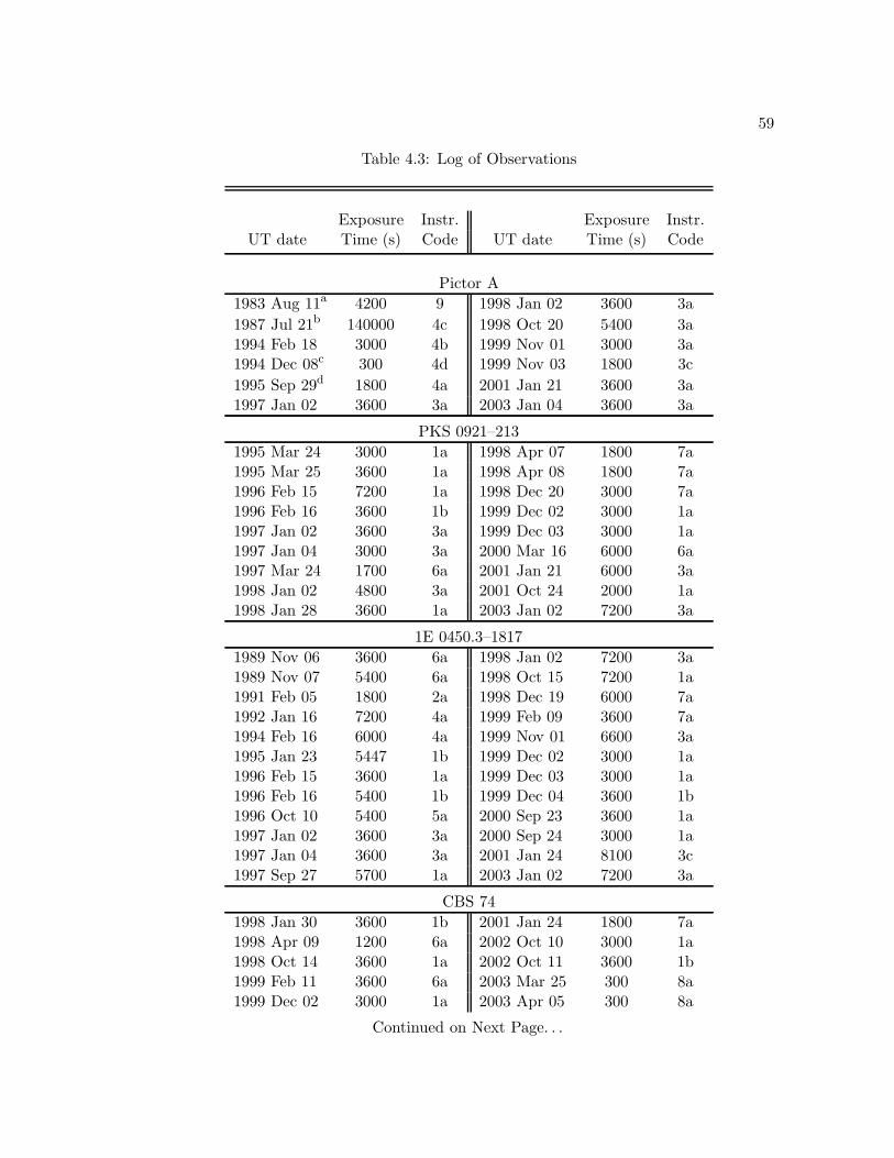
59

Table 4.3: Log of Observations

Exposure Instr. Exposure Instr.UT date Time (s) Code UT date Time (s) Code

Pictor A

1983 Aug 11a 4200 9 1998 Jan 02 3600 3a

1987 Jul 21b 140000 4c 1998 Oct 20 5400 3a1994 Feb 18 3000 4b 1999 Nov 01 3000 3a1994 Dec 08c 300 4d 1999 Nov 03 1800 3c

1995 Sep 29d 1800 4a 2001 Jan 21 3600 3a1997 Jan 02 3600 3a 2003 Jan 04 3600 3a

PKS 0921–213

1995 Mar 24 3000 1a 1998 Apr 07 1800 7a1995 Mar 25 3600 1a 1998 Apr 08 1800 7a1996 Feb 15 7200 1a 1998 Dec 20 3000 7a1996 Feb 16 3600 1b 1999 Dec 02 3000 1a1997 Jan 02 3600 3a 1999 Dec 03 3000 1a1997 Jan 04 3000 3a 2000 Mar 16 6000 6a1997 Mar 24 1700 6a 2001 Jan 21 6000 3a1998 Jan 02 4800 3a 2001 Oct 24 2000 1a1998 Jan 28 3600 1a 2003 Jan 02 7200 3a

1E 0450.3–1817

1989 Nov 06 3600 6a 1998 Jan 02 7200 3a1989 Nov 07 5400 6a 1998 Oct 15 7200 1a1991 Feb 05 1800 2a 1998 Dec 19 6000 7a1992 Jan 16 7200 4a 1999 Feb 09 3600 7a1994 Feb 16 6000 4a 1999 Nov 01 6600 3a1995 Jan 23 5447 1b 1999 Dec 02 3000 1a1996 Feb 15 3600 1a 1999 Dec 03 3000 1a1996 Feb 16 5400 1b 1999 Dec 04 3600 1b1996 Oct 10 5400 5a 2000 Sep 23 3600 1a1997 Jan 02 3600 3a 2000 Sep 24 3000 1a1997 Jan 04 3600 3a 2001 Jan 24 8100 3c1997 Sep 27 5700 1a 2003 Jan 02 7200 3a

CBS 74

1998 Jan 30 3600 1b 2001 Jan 24 1800 7a1998 Apr 09 1200 6a 2002 Oct 10 3000 1a1998 Oct 14 3600 1a 2002 Oct 11 3600 1b1999 Feb 11 3600 6a 2003 Mar 25 300 8a1999 Dec 02 3000 1a 2003 Apr 05 300 8a

Continued on Next Page. . .

60

Table 4.3 – Concluded

Exposure Instr. Exposure Instr.UT date Time (s) Code UT date Time (s) Code

1999 Dec 04 3000 1b 2003 Oct 24 1800 7a2000 Mar 14 6000 6a 2003 Dec 24 1200 8a2000 Sep 24 3000 1b 2004 Jan 13 300 8a

3C 59

1991 Feb 04 1800 2a 2000 Sep 24 3600 1b1991 Feb 05 1500 3a 2001 Jul 21 2700 1b1997 Feb 07 3000 1a 2002 Oct 10 3600 1a1997 Sep 28 3600 3a 2002 Oct 11 3600 1b1998 Oct 13 3600 3a 2003 Oct 21 600 8a1998 Oct 15 3600 1a 2004 Jan 19 600 8a1998 Dec 20 2400 7a 2004 Sep 09 600 8a1999 Dec 04 3600 1b · · · · · · · · ·

PKS 1739+18C

1992 Jul 09 1800 2a 2000 Jun 04 2400 1b1996 Jun 15 3600 1b 2000 Sep 24 2400 1b1997 Jun 09 3600 1b 2001 Jul 21 3000 1b1997 Sep 28 3600 1b 2002 Jun 14 2700 1b1998 Apr 09 3000 7b 2002 Oct 11 3600 1b1998 Jun 27 3000 7a 2003 Apr 02 300 8a1998 Oct 13 3600 1b 2004 Jun 22 300 8a1999 Jun 15 3000 1b 2004 Aug 05 300 8a

PKS 1020–103

1991 Feb 04 600 2a 1998 Jan 05 3600 3a1991 Feb 05 2400 2a 1998 Dec 20 2400 7a1992 Jan 16 1800 4a 1999 Dec 04 3600 1a1996 Feb 16 3600 1a 2001 Jan 22 7200 3d1997 Jan 04 3600 3a 2003 Jan 03 6000 3d

aKindly provided in reduced form by A. V. Filippenko, see Filippenko (1985)

bSum of seven exposures over three nights, 1987 Jul 20-22. Kindly provided by S. Simkin (see

also, Sulentic et al. 1995).cKindly provided in reduced form by T. Storchi-Bergmann.

dKindly provided in reduced form by R. H. Becker.

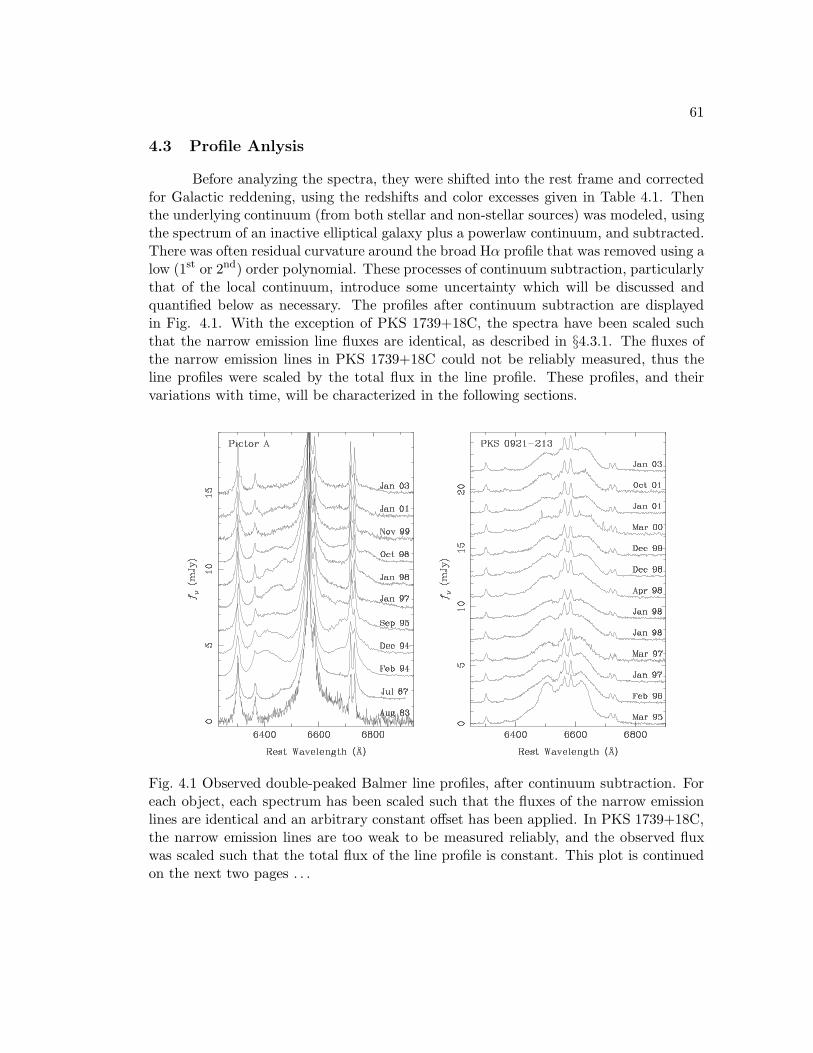
61

4.3 Profile Anlysis

Before analyzing the spectra, they were shifted into the rest frame and correctedfor Galactic reddening, using the redshifts and color excesses given in Table 4.1. Thenthe underlying continuum (from both stellar and non-stellar sources) was modeled, usingthe spectrum of an inactive elliptical galaxy plus a powerlaw continuum, and subtracted.There was often residual curvature around the broad Hα profile that was removed using alow (1st or 2nd) order polynomial. These processes of continuum subtraction, particularlythat of the local continuum, introduce some uncertainty which will be discussed andquantified below as necessary. The profiles after continuum subtraction are displayedin Fig. 4.1. With the exception of PKS 1739+18C, the spectra have been scaled suchthat the narrow emission line fluxes are identical, as described in §4.3.1. The fluxes ofthe narrow emission lines in PKS 1739+18C could not be reliably measured, thus theline profiles were scaled by the total flux in the line profile. These profiles, and theirvariations with time, will be characterized in the following sections.

Fig. 4.1 Observed double-peaked Balmer line profiles, after continuum subtraction. Foreach object, each spectrum has been scaled such that the fluxes of the narrow emissionlines are identical and an arbitrary constant offset has been applied. In PKS 1739+18C,the narrow emission lines are too weak to be measured reliably, and the observed fluxwas scaled such that the total flux of the line profile is constant. This plot is continuedon the next two pages . . .

62

Figure 4.1 continued . . .

63

Figure 4.1 concluded.

64

4.3.1 Relative Narrow and Broad Line Fluxes

The absolute flux scale is uncertain by up to a factor of two, because the spectrawere observed though a narrow slit and in variable sky conditions. A technique commonlyused in studies of AGN broad line variability is to use the narrow emission lines forinternal flux calibration. These lines form in low-density gas located several light decadesfrom the central engine and they are not expected to respond to rapid variations incontinuum flux (see, e.g., Peterson 1993). The narrow emission lines covered by thesespectra include [O i]λλ6300,6363, [N ii]λλ6548,6583, [S ii]λλ6716,6730, and the narrowcomponent of Hα. Scaling factors are determined for each spectrum to achieve a uniformflux scale for all of the spectra, relative to a chosen reference spectrum.

Unlike the narrow emission lines, the total flux in the broad Hα line does varyin response to changes in the external illumination. It is important to determine howthe total broad Hα flux changes with time, again relative to some reference spectrum,for two reasons. Firstly, if one wants to study variations in the shape of the broadHα line profiles, it is necessary to scale the profiles such that they have the same totalbroad Hα flux. Short-term fluctuations in the illumination will cause the total broadline flux to change (i.e. through light reverberation), as observed in 3C 390.3 (Dietrich1998; Shapovalova et al. 2001). These changes in flux are not of interest when studyinglong-term profile variability that is due to physical changes in the accretion disk, andmust be corrected for. Secondly, as discussed in more detail in §4.3.4, the propertiesof the double-peaked line profile may vary in response to long-term variations in theilluminating flux, for example as seen in NGC 1097 (Storchi-Bergmann et al. 2003); itwould be interesting to see if such effects are common in other objects.

To measure the fluxes of the narrow lines, the underlying broad Hα profile mustbe subtracted. The [O i]λ6300, [O i]λ6363 and [S ii]λλ6716,6730 lines lie on the wings

of the broad Hα profile, which are well approximated by a 3rd order polynomial. Thereis typically less than a 10% difference between the fluxes of the strong [O i]λ6300 and[S ii]λλ6716,6730 lines obtained for different fits to the wings of the broad Hα profile,however the weaker [O i]λ6363 line flux has a larger (∼ 20%) uncertainty.

Fitting the [N ii]λλ6548,6583 and narrow Hα lines is more challenging for tworeasons. The [N ii]λλ6548,6583 lines can be blended with Hα, but this difficulty is easilyovercome. The [N ii] lines are fitted first, with the assumption that the [N ii]λ6583 lineflux is three times larger than that of [N ii]λ6548, as dictated by atomic physics, and thatthe FWHM of the line profiles are identical. After the [N ii] lines are subtracted, theresidual Hα flux is easily determined. In some objects, there are clearly two componentsof narrow Hα, one with a FWHM similar to that of the forbidden lines (∼ 1000 km s−1)

and another (sometimes blue-shifted) with a FWHM of ∼ 2000–3000 km s−1; the fluxesof both components are included in the narrow line flux. The line decomposition is quiterobust and for a given fit to the underlying broad Hα profile and the uncertainty in thenarrow Hα and [N ii] fluxes is similar to that for [O i] and [S ii] (∼ 10–15%).

Of greater concern is the fact that any fit to the underlying broad Hα profileis necessarily based upon an assumption about the general shape of the broad profile.Thus the Hα and [N ii] flux measurements are subject to systematic uncertainty. Usinga few test spectra, the effective continuum underlying the Hα+[N ii]narrow line was

65

subtracted using a number of different models and the line fluxes of the residual narrowlines were measured as described above. Not all fits to the underlying broad Hα profilelead to reasonable Hα+[N ii] residuals; the [N ii] lines must be fitted with a flux ratio of3:1 and the remaining Hα profile must be approximately fitted by one or two Gaussianprofiles. Within this constraint, the systematic uncertainty due to fitting the broadprofile was estimated to be approximately 30%.

It is possible to guard against this systematic uncertainty by considering the ratiosof the narrow line fluxes (i.e. [O i]/[S ii], [S ii]/Hα, [O i]/Hα, and [N ii]/Hα), which likethe narrow line fluxes, should not change significantly with time. These line ratios arevery stable from one observation of an object to the next, with only a handful of outliers.If the fit to the underlying broad Hα profile were wildly different from one observationto the next, this would be manifested in the line ratios, with the exception of [O i]/[S ii].It is still possible that the Hα+[N ii] flux can be systematically uncertain by up to30%, however as long as the flux is systematically under- or over-estimated by roughlythe same amount for all of the observations, this systematic uncertainty will have littleeffect on the relative broad line fluxes.

The narrow line scaling factor was determined for each spectrum by dividing themeasured narrow line fluxes by those from a reference spectrum. The scaling factors fromthe individual lines were averaged together, and the standard deviation of the values wasassigned as an approximate error bar. The individual scaling factors generally lay withintwo standard deviations (and in most cases within 1 standard deviation) of the mean.In a few instances an individual scaling factor, typically from Hα or [N ii], was clearlyskewing the mean; this point was eliminated and the mean and standard deviation wererecalculated. The fractional uncertainty in the narrow line scaling factors was typically10–15%.

To determine the broad line scaling factor, the total narrow line flux determinedabove was subtracted from flux of the entire profile (narrow + broad). The local contin-uum subtraction introduces a 5–10% uncertainty in the flux of the total profile, but doesnot introduce any additional uncertainty into the total narrow line flux. The broad linescaling factor is simply the ratio of the total observed broad line flux for each observationdivided by that for the reference spectrum. When all the errors are taken into account,the uncertainty on the broad line scaling factors are less than 10% for all objects.

Given that there are 15% and 10% fractional errors on the broad and narrow linescale factors, respectively, the “true” broad line fluxes, relative to a reference spectrum,are generally uncertain by ∼ 20%. In Fig. 4.2, the broad Hα lightcurves are shown.Despite the large uncertainty in the broad Hα fluxes, there are several objects (1E 0450.3,Pictor A, and PKS 0921-213) for which there are obvious variations in the broad Hαflux; the impact of this varying broad Hα flux on the profile shape is explored in §4.3.4.

In the next two sub-sections, I present two different methods for characterizing thevariations in double-peaked line profiles in a model-independent way. After the resultsfor each method are presented, I first describe general trends and then highlight resultsfrom specific objects.

66

Fig. 4.2 Variations in the total broad Hα flux as a function of time, relative to a particular observation. The relative fluxes andtheir errors were calculated as described in §4.3.1.

67

4.3.2 Difference Spectra

One simple way to visualize how a line profile is changing with time is to createdifference spectra, in which one plots the residuals from some reference spectrum. HereI present difference spectra that result from subtracting either the average or the “min-imum” profile. The former is simply the average of all the profiles whereas the latteris constructed by selecting, at each wavelength, the minimum flux from among all thespectra. This minimum spectrum represents a base profile which is common to all theprofiles. As an idealized example, if the emission arises from a circular accretion diskwith an emissivity enhancement (such as a hot spot or spiral arm), then the minimumprofile would be that of the underlying circular accretion disk, and the difference spectrawould clearly reveal the emissivity enhancement as it travels through the disk and affectsdifferent portions of the emission line profile.

Before constructing the difference spectra, the original spectra were renormalizedto the same total broad line flux (see §4.3.1). This procedure eliminates the effects oflarge changes in the total illumination (such as those observed in 3C 390.3 due to lightreverberation Dietrich 1998; Shapovalova et al. 2001) that would obscure changes in theprofile shape. The spectra were also resampled to the wavelength scale of the spectrumwith the highest spectral resolution (typically 3A), so they could be subtracted pixel-by-pixel. Then the two “comparison” spectra were subtracted from each individualspectrum. The resulting difference spectra are shown in Fig. 4.3. Because the spectrawere rescaled to have similar broad-line fluxes, the narrow emission lines fluxes varyfrom one observation to the next. Rather than remove the narrow lines, which wouldrequire assumptions about the shape of the underlying profile, these regions were simplynot plotted in the difference spectra and the omitted regions are indicated by verticalgray stripes. As can be seen in Fig. 4.3, the prominent features in the difference spectraare generally broader than the omitted spectral regions, thus these gaps do not greatlyimpair the interpretation of the difference spectra.

There are several trends commonly seen in the difference spectra of most objects.In general, trends are best illustrated by the differences from the minimum spectrum.

1. The difference spectra reveal the presence of distinct lumps of emission, and typi-cally there are multiple lumps, sometimes at both negative and positive projectedvelocities, at any given time. The amplitude of these lumps, relative to the flux inthe minimum spectrum at the position of the lump, is typically 20–30% althoughwhen the lump is located at the wings of the profile, the relative flux is muchlarger (∼ 50%). An exception is Pictor A, in which the spectrum has undergonesignificant changes in profile shape; the flux in the “lumps” of emission is severaltimes larger than in either the minimum or the average spectrum. The changes inthese distinct lumps of excess emission, either in shape, amplitude, or projectedvelocity, are primarily responsible for the variability in the line profiles.

2. Neither the average nor, more importantly, the minimum spectra are consistentwith the expected profile from a circular accretion disk, because the red peak isoften as strong as, or stronger, than the blue peak. If the profile variability canindeed be explained as an underlying disk with extra, transient lumps of emission,

68

Fig. 4.3 Difference between each individual spectrum and either the average or minimumspectrum, as described in §4.3.2. The average or minimum profile is shown on the top,and the difference spectra are stacked below. Please note that the time interval betweeneach spectrum is not uniform. The vertical gray stripes indicate regions of the spectrumoccupied by narrow emission lines which are not being plotted for clarity. The dottedhorizontal line indicates the null flux level for each spectrum. A dotted vertical linein the spectra of PKS 1739+18C indicates the position of the B-band. This figure iscontinued over the next five pages . . .

69

Figure 4.3 continued . . .

70

Figure 4.3 continued . . .

71

Figure 4.3 continued . . .

72

Figure 4.3 continued . . .

73

Figure 4.3 concluded.

then the underlying disk itself cannot be modeled as an axisymmetric disk andthus the “base” (i.e. minimum) profile can be expected to vary on long timescales.Thus one should be cautious in associating the minimum spectrum with the profileof an underlying “static” disk to which all other features are added.

3. The less luminous systems – Pictor A, PKS 0921–213, and 1E 0450.3–1817, varyon shorter timescales than the more luminous systems that presumably have moremassive black holes. The three lowest redshift objects have known black holemasses (MBH ∼ 4 × 107M), determined in Chapter 2, and will be discussed inmore detail in §4.5.

4. If one assumes that lumps from one observation epoch can be tracked in followingobservations, several general conclusions can be drawn.

(a) The lumps can persist for several years; in a few objects, some lumps appearto remain throughout the duration of the monitoring observations such as thered lumps in 3C 59 and PKS 1739+18C. These lumps still do vary slightly inamplitude and shape, but they do not dissipate completely.

(b) When the lumps are variable, they typically arise on rather short timescales(less than one year) and dissipate more slowly (over several years), generallybecoming broader in the process of decaying. In an extreme case, a lumpdisappeared on timescales of less than a year, and a new one appeared in

74

approximately the same place within another year (e.g. 1E 0450.3–1817, 1995–1996).

(c) The lumps are often observed to drift across the profile from positive to nega-tive projected velocity and only very rarely does the lump drift in the oppositesense, reminiscent of Arp 102B (Sergeev et al. 2000; Gezari 2005).

Pictor A, PKS 0921–213, 1E 0450.3–1817 and CBS 74 all show striking variabilitywhich I describe in more detail here.

Pictor A. – This object shows the most dramatic variability, in the sense thatthe line was not observed to be double-peaked prior to 1994. The bluepeak originated at a projected velocity of ∼ 7500 km s−1, implying thatthe emitting gas is located at characteristic radius (rc) of less than 1500 rg[(rc/rg)

−1/2 ∼ v/c]. This peak steadily drifted to less negative projected ve-

locity (∆vp ∼ 3000 km s−1) over a period of approximately 4 years and hasbeen dissipating slowly over at least 7 years (the blue peak is still presentin the last observation epoch). It is interesting to note that the red peakemerged earlier than the blue peak, and has all but disappeared at the lastobservation epoch.

PKS 0921–213. – The profile of this object in the early observations is veryunusual and appears to have two double-peaked components, one with morewidely separated peaks underlying another with more closely spaced peaks.This latter component appears to have mostly disappeared within a year.After this, the most prominent feature is a lump in the red peak, at a pro-jected velocity of ∼ 4500 km s−1 (implying a characteristic radius of less than4000 rg) that strengthened over two years and also began to dissipate overa similar timescale. Additionally during this time, the lump drifted towardslower projected velocity by ∼ 2000 km s−1.

1E 0450.3–1817. – This object is unique in the large number of distinct lumpswhich have appeared, drifted across the profile, and dissipated; during someobservation epochs there are up to three different lumps present at once. Thelumps emerged at both small and large (as well as negative and positive)projected velocities. Some of the lumps are long-lived and do not vary sig-nificantly in strength, shape, or position over a period of ∼ 8 years, whereasother lumps emerge, drift, and dissipate over 4 years.

CBS 74. – A lump located in the red side of the profile drifted by 2000 km s−1

(projected velocity) and dissipated over approximately two years. A secondbroad feature on the blue side of the profile steadily increased in strength andthen began to decrease again over 5 years. The rapid variability in this objectmay be related to the fact that the inner radius of the disk extends down to∼ 200 rg. Although the black hole mass is probably larger in this object thanin Pictor A, PKS 0921–213, and 1E 0450.3–1817, the physical timescales forvariability may be similar.

75

In the above descriptions, I have assumed that one can track a lump from oneepoch in subsequent observations. This does not imply that the same parcel of gas isresponsible for the emissivity enhancement and in fact this cannot be the case, at leastfor PKS 0921–213 and 1E 0450.3–1817. The dynamical timescales for these objects areknown to be only a few months (see Chapter 2) and each of these objects were closelymonitored at times (with gaps of only 1–2 months between observations); there wasclearly no orbital motion. Thus, these lumps of emission should not be likened to thebright spot postulated by Newman et al. (1997). The fact that the properties of thelumps (projected velocity, width, and amplitude) are not randomly distributed from oneobservation to the next strongly suggests some kind of physical connection between theselumps, but the lumps are associated with a location in the disk, rather than any particularparcel of matter within the disk. I offer a possible interpretation of this phenomenon in§4.5

4.3.3 Variations in Profile Parameters

As shown in §4.3.2, difference spectra are powerful tools for diagnosing the rootcause of the observed variability, such as an emissivity enhancement that is travelingacross the profile or the sudden dissipation of a feature. However, it is also desirable tocharacterize the data in a more quantitative way. In particular, even if a given family ofmodels is able to qualitatively reproduce the observed profiles, there is a large region ofparameter space to be explored in order to find the best-fitting model for a sequence ofprofiles; a quantitative description of the profile variations will be of great utility whendetailed modeling is performed.

Although the profiles are extremely complex, to first order they can be reduced toa small set of easily measurable quantities: the velocity shifts of the red and blue peaks,the ratio of the blue to red peak flux, the full-width of the profile at half-maximum andquarter maximum (FWHM and FWQM), the velocity separation of the two peaks, thevelocity shifts of the profile centroid at FWHM and FWQM, and the average velocityshift of the peaks. The maximum is defined to be the flux of the higher peak and allvelocities are measured with respect to the narrow Hα emission line. The resulting plotsof profile parameters as a function of time are shown in Fig. 4.4.

In determining the profile parameters for a given spectrum, there are three majorsources of uncertainty. First and foremost is the error in measuring the various parame-ters. The velocity shifts of the red and blue peaks and the shifts of the profile at FWHMand FWQM can be quite uncertain. For example, when a peak is flat-topped, such asthe blue peak of PKS 1739+18C, there is considerable ambiguity in the location of thepeak. In objects where the peak fluxes are relatively low, or the [S ii]λλ6716, 6731 and[O i]λ6363 lines are strong, the profile at the half- and/or quarter-maximum is contam-inated by these narrow lines, making it difficult to determine the width and especiallythe shifts of the profile. To take into account this uncertainty, each profile propertywas measured three times, the values were averaged and the standard deviation in themeasurements was assigned as an error bar. In some objects (1E 0450.3–1817, PKS 0921–213), and CBS 74), there appear to be multiple peaks in a small number of spectra andin all cases the stronger peak (which was also had the less extreme projected velocity)

76

was adopted rather than measuring the positions of both peaks and assigning extremelylarge errors to the peak position and flux ratio.

In addition, continuum subtraction introduces additional uncertainty in the mea-sured profile properties, particularly in the FWHM and FWQM. It was not practicalto explore the effect of continuum subtraction for each spectrum individually. Instead,the effects of continuum subtraction were explored in great detail for two representativespectra, one from PKS 0921–213, which has a large starlight fraction, and one from PKS1739+18C, which has a negligible contribution from starlight. The errors incurred fromcontinuum subtraction were very similar for both of these objects, and this extra errorwas adopted for the other spectra, for which only a set of three measurements was made.As a consistency check, for a few spectra from each object the local continuum subtrac-tion was performed several times to ensure that the error from the continuum subtractionwas similar to what was estimated from the test cases. When the error for a particu-lar object was larger than in the test cases, the error bars were increased accordingly.Additionally, a few objects were observed multiple times within a few days, thus it wasalso possible to estimate the errors that are induced by different observing conditions.This error is relatively small compared to those from continuum subtraction and themeasurement process, but not negligible. When multiple spectra were obtained withinone month of each other, the results were averaged together, and in these instances itwas not necessary to factor in this latter error.

The variability plots reveal a few additional trends, which were not readily ap-parent from the difference spectra presented in §4.3.2.

1. Blueshifts in the profile of the FWHM, FWQM and the average peak velocity arequite common, and the blueshifts can be as large as 2000 km s−1, although theyare more typically ∼ 500 km s−1. There is also considerable variability in theseshifts.

2. With the exception of the profile widths at FWHM and FWQM, the various pa-rameters rarely vary in concert. In some objects the peak separation varies in asimilar way as the profile widths, but not in all instances.

3. It is not uncommon for the red peak to be stronger than the blue peak. Withthe exception of CBS 74, for which the Doppler boosting of the blue peak is quitestrong, all of the objects in this sample have a red peak that is stronger thanthe blue in at least 50% of the observations! I note that due to the non-uniformsampling, this does not imply that the red peak is stronger than the blue 50% ofthe time. More puzzling is that in some cases the peak reversal is extreme, withthe red peak being 20-30% stronger than the blue. The most striking instancesof a peak reversal are PKS 0921-213 and Pictor A, in which the blue peak hasat best achieved a flux equal to that of the red peak. In the context of a diskmodel, a rather dramatic asymmetry is required to produce such a strong peakreversal. If this asymmetry is persistent, then objects which exhibit these strongred peaks should, at some epoch exhibit, extremely large ratios of the blue tored peak flux, especially considering that any asymmetry in the emissivity willbe Doppler boosted on the blue side. These objects may simply have not been

77

Fig. 4.4 Variations in the profile properties: (1) the velocity shift of the red and bluepeak, (2) the ratio of the blue to red peak flux ratio, (3) the full-widths at half andquarter maximum and the peak separation (denoted by open red triangles, filled bluecircles, and filled black stars, respectively) (4) and the velocity shift of the profile atthe FWHM, FWQM and the average peak velocity offset. All velocities are referencedwith respect to the narrow Hα emission line. The measurement procedure is describedin §4.3.3. This figure is continued on the next two pages . . .

78

Figure 4.4 continued . . .

79

Figure 4.4 concluded.

observed over a long enough time period to observe large blue peak fluxes yet,however the lack of strong blue peaks is very curious.

4.3.4 Variations with Integrated Broad Hα Flux

As mentioned in §4.3.1, variations in the illuminating flux might lead to variationsin the line profiles. The accretion disk itself is not truncated at the inner and outerradii, rather these regions do not emit Balmer emission lines efficiently because the gasis over-ionized or not adequately illuminated. Thus the effective inner and outer radiiare not rigid and may be influenced by the changes in the illuminating flux. Thus, as theilluminating flux increases, the inner and outer radii might become larger; this will resultin a decrease in the peak separation. The profile widths at FWHM and FWQM are alsoaffected, but changes in the peak ratio and the line profile shifts are less pronounced. Theerrors on the FWHM and FWQM are generally quite large, thus I focused on searchingfor negative correlations between variations in the peak separation and the broad Hαflux. Such correlations have in fact been observed in NGC 1097 (Storchi-Bergmann et al.2003), 3C 332 (Gezari 2005), and also possibly 3C 390.3 (Shapovalova et al. 2001). Fourof the seven objects (Pictor A, PKS 0921–213, 1E 0450.3–1817, and PKS 1020–103) showvariability in the broad Hα flux, and in Fig. 4.5 the peak separation as a function of thebroad Hα flux is shown for these objects.

80

Fig. 4.5 Variations in the velocity separation of the red and blue peaks as a functionof the relative broad Hα flux, as determined in §4.3.1, for Pictor A, PKS 0921–213,1E 0450.3–1817, and PKS 1020–103. Each data point is labeled with the observationnumber. In some instances two observations overlap, and only one data point is visible.

81

As can be seen in Fig. 4.5, there is no clear correlation between variations in thepeak separation and the broad Hα flux. In many instances there are dramatic variationsin either the peak separation or flux, without a corresponding variation in the other. Forexample, the most dramatic variations in the peak separation in Pictor A occur from1994 to 1997, when the broad Hα flux is nearly constant.

In PKS 0921–213, the flux decreases by a factor of two from 1995 March to 1997March, and it is suggestive that the profile changes dramatically over this time period.However, the peak separation actually increases over this interval. As described in §4.3.2above, the initial spectrum of PKS 0921-213 (1995 March) may actually have two double-peaked components, one with a lower flux level and broader peaks and a second withnarrower peaks, the latter of which seems to disappear over the course of the next severalobservations. If this is indeed the case, the peaks which should be measured are those ofthe persistent, lower-flux component, not those of the transient component, as has beendone. Therefore the peak separations determined for the initial several spectra may beincorrect. If one considers only the last five observations, there is a hint of a negativetrend between the broad Hα flux and the peak separation. However, this is a verytentative conclusion, and the correlation could be spurious, particularly in light of thefact that this phenomenon was not noticed in any of the other objects. The variations inthe flux of the illuminating continuum most likely have impacted the shape of the profilein PKS 0921–213, but the simple model in which the inner radius of the disk increaseswith flux probably does not apply.

4.4 Model Profile Characterization

In this section I characterize the profile variability of two families of models—anelliptical disk and a circular disk with a spiral emissivity perturbation—which have beenused in the past to model the profile variations in some double-peaked emitters (see§4.1.) Although these models are simple, there is strong theoretical motivation for each;they are not simply convenient ways to “parameterize” the observed profile variability.Thus before describing the details of the profile calculation (§4.4.2) and the variabilitypatterns for these models (§4.4.3), I set the stage by describing the mechanisms whichcould lead to the formation of elliptical disks and disks with spiral arms.

4.4.1 Physical Motivation

Elliptical Disk – An elliptical accretion disk could form due to the presence of a secondsupermassive black hole, analogous to the formation of an elliptical disk in someCVs due to perturbations from the companion star (see the discussion of Eracleouset al. 1995). Because galaxies (and in particular the massive early-type galaxiesthat typically host radio galaxies) are thought to form through mergers, it is likelythat some galaxies contain binary black holes pairs (Begelman, Blandford, & Rees1980). These authors estimated that for conditions similar to those found in thecores of massive ellipticals, the black holes in the two merging galaxies wouldquickly form a “hard” state binary. The binary will remain hard for a long time(108–1010 years) because eventually the stars in the central regions of the galaxy

82

that are capable of interacting with the binary, leading to further hardening, willbe depleted. The timescale for hardening is then controlled by the rate at whichstars refill the loss cone, i.e. the relaxation time. This idea has been recentlyconfirmed by large N-body simulations by Makino & Funato (2004). Due to thecontinuous perturbation by the second black hole, the accretion disk around theprimary will quickly attain a uniform eccentricity and maintain that eccentricityfor some time. Alternatively, if the accretion disk is only perturbed temporarilyby a massive body, the inner regions of the disk will begin to circularize due todifferential precession.

A second formation mechanism for an elliptical disk suggested by Eracleous et al.(1995), inspired by the sudden appearance of double-peaked emission lines in theLINER NGC 1097, is the tidal disruption of a star by a black hole. For a blackhole with a MBH . 108M, a solar-mass star will be tidally disrupted before it isaccreted. This tidal debris initially has very eccentric orbits, and Syer & Clarke(1992) find that the debris will form an eccentric accretion disk within a viscoustimescale.

Spiral Arms. – The second model I consider is that of a circular disk with a spiralemissivity perturbation which is an attractive model for numerous reasons. Firstly,spiral arms are directly observed in galactic disks and indirectly CVs (see, e.g.,Steeghs, Harlaftis, & Horne 1997; Baptista, Harlaftis, Marsch, & Steeghs 2005;Papadimitriou, Harlaftis, Steeghs, & Niarchos 2005). Spiral waves are thoughtto form in CVs due to tidal interactions with the binary companion whereas inself-gravitating galaxy disks they form due to gravitational instabilities. In AGNaccretion disks, only the outer portions (ξ ≥ 1000 rg) are self-gravitating. Howeverthe passage of a massive star cluster, a second supermassive black hole, or eventhe effects of a triaxial stellar distribution could induce the formation of a spiralarm. Chakrabarti & Wiita (1993, 1994) first suggested that spiral shocks might bea major contributor to the variability in the double-peaked emission lines in CVsand AGNs (Arp 102B and 3C 390.3), respectively. Secondly, spiral arms can play arole in angular momentum transport (see, e.g, Livio & Spruit 1991; Matsuda et al.1989). In particular, other proposed mechanisms for angular momentum transport(i.e. “viscosity” and hydromagnetic winds) may be ineffective in the outer diskand an alternative mechanism such as a spiral arm may be necessary. Finally,Chakrabarti & Wiita (1993) suggest that spiral shocks in an accretion disk maycontribute to the photometric variability commonly observed in AGNs because thespiral shocks fragment and reform, naturally leading to the formation of transitory“hot spots” on the disk.

In all of the scenarios presented above, either the eccentric disk or the spiral armwill precess on long timescales, leading to variability in the observed line profile. Thetimescales over which the variability is expected is discussed further in §4.5.

83

4.4.2 Calculation of the Model Profiles

The symmetric double-peaked emission lines seen in CVs result from the red- andblueshifting of the emission line arising from different portions of the rotating accretiondisk. When the emission from the entire disk is considered, there is comparativelylittle gas traveling with very small or very large projected velocity, and most of theemission arises from gas that is moderately red- or blueshifted. The line profile from anAGN accretion disk is affected by several relativistic effects. These include (1) Dopplerboosting of the blue peak relative to the red peak, (2) gravitational redshifting, whichshifts the entire line profile to longer wavelengths and can cause the red wing of the lineto become extended and (3) light bending, that leads to a solid angle (and thus flux) thatchanges with the radius in the disk and the inclination of the disk with respect to thethe observer. Although these relativistic effects make it more difficult to compute theline profile, they effectively break the degeneracies between the inner and outer radiusand the inclination angle that are problematic in the study of CVs.

A formalism for calculating the double-peaked emission line profiles in the weak-field limit was laid out by Chen et al. (1989) and Chen & Halpern (1989). The lineprofile is computed numerically by integrating:

fν ∝∫

ξdϕ

∫

dξ Iν(ξ, ϕ, ν) D3(ξ, ϕ) Ψ(ξ, ϕ) (4.1)

over the surface of the disk. Here, ϕ is the azimuthal angle in the frame of the disk and ξis the distance from the central black hole in units of rg. The emissivity of the disk andinformation about the local line profile are given in Iν(ξ, ϕ, ν). The velocity structureof the disk is contained in D(ξ, ϕ), the Doppler factor, and gravitational redshifting andlight bending are incorporated through Ψ(ξ, ϕ). It is important to note that the weak-field approximations made in this calculation are invalid for ξ . 100 (see, e.g., Fabianet al. 1989). The codes used to implement both the elliptical and spiral-arm models forthe line profiles are the same as those used by Storchi-Bergmann et al. (2003).

For an elliptical disk, the Doppler factor was recomputed by Eracleous et al.(1995) to account for the non-circular orbits. The specific intensity is given by:

Iν =1

4π

ε0ξ−q

√2πσ

exp

[

−(νe − ν0)2

2σ2

]

(4.2)

where the exponential term accounts for local broadening of the emission line due toturbulence and the factor of ξ−q accounts for the decrease in incident flux from theilluminating source. The value of q lies between 1–3 (see, e.g. Chen & Halpern 1989;Dumont & Collin-Souffrin 1990b; Strateva et al. 2003; Eracleous & Halpern 2003). Theelliptical disk model used here has seven parameters: ξ1 and ξ2, the inner and outerpericenter of the line-emitting region, the inclination angle i (i ≡ 0 for a face-on disk), thebroadening parameter σ, and the eccentricity which is described with three parameters—e1, e2, and ξe. The disk has an eccentricity e1 from ξ1 to ξe and from ξe to ξ2, theeccentricity increases linearly from e1 to e2. Thus a wide range of disks can be described,from disks with constant eccentricity to those in which the inner regions have circularized.

84

Time evolution of the profiles via precession of the elliptical disk is achieved by varyingthe angle that the major axis makes to the line of sight (φ).

The spiral arm model was implemented by introducing an emissivity perturbationwith the shape of a spiral arm, given by:

Iν(ξ, φ) = I0

ν (ξ)

1 +A

2exp

[

4 ln2

δ2(φ− ψ0)

2

]

+A

2exp

[

4 ln2

δ2(2π − φ+ ψ0)

2

]

(4.3)

where I0

ν(ξ) is given by Eqn. 4.2 and

ψ0 = φ0 +log(

ξ/ξsp)

tan p. (4.4)

Here ξ1 and ξ2 represent the inner and outer radius and q, i and σ are the sameas above. The spiral perturbation introduces several additional parameters: A, theamplitude of the arm (i.e. the contrast relative to the underlying disk); the pitch angle,p; the angular width of the arm, δ; and the termination radius of the arm, ξsp (the arm islaunched from the outer edge of the disk). Again time variability is achieved by varyingthe viewing angle φ. In CVs, pairs of spiral arms are often observed, however Gilbertet al. (1999) found that the presence of multiple spiral arms led to a disk which was toosymmetric to reproduce the peak reversals observed in 3C 332 and 3C 390.3. Moreover,a single armed spiral is preferred in a disk that has a Keplerian rotation curve in theabsence of an external tidal perturbation (Adams, Ruden, & Shu 1989). In principle,one should alter the Doppler factor to account for the perturbation to the velocity fieldas well, as was done by Chakrabarti & Wiita (1994). Using time-resolved spectroscopyand eclipse mapping of the CV IP Pegasi, Baptista et al. (2005) found that the velocitiesalong the two spiral arms (which are located at different distances from the center) arelower than the Keplerian velocity by up 10-15% in the distant arm and 40% lower in thecloser arm.

4.4.3 Model Characterization

Rather than fitting these models directly to the observed profiles, I have charac-terized extensive libraries of these model profiles in exactly the same way as for the data,namely the construction of difference spectra and plots of the profile parameters as afunction of time. A few representative examples from the library of models are shownin Fig. 4.6. In each, the primary disk parameters (ξ1, ξ2, i, σ) were chosen to specifi-cally match some of the objects being studied here to facilitate a comparison. However,the other properties were chosen simply for illustration. Only the differences from theminimum spectra are shown. The elliptical disk model leads to surprisingly similar dif-ference spectra and patterns in the profile parameter variations over a wide range ofmodel parameters, thus only one example is shown. The amplitude of the variations arecertainly dependent on specific model parameters, but the general trends are not. Onthe other hand, the spiral arm models exhibit more diverse variability patterns, and alarger number of examples are shown.

85

Fig. 4.6 Left: Grayscale image of the disk emissivity. Center: Differences from the minimum spectrum at various precessionphases. The model parameters are listed at the top of this panel; for a description of the models and their input parameters,please see §4.4. The inner and outer radii, inclination angle, and powerlaw illumination index, and broadening parameter werechosen to approximate the profile of PKS 0921–213, however the eccentricity and ξe were chosen simply for illustration.Right:Plot of profile parameters as a function of precession phase, identical to those in Fig. 4.4. Here the profile widths at FWHM,FWQM, and the peak separation (as well as the corresponding profile shifts) are represented by solid, dashed, and dotted lines,respectively. This figure is continued with examples for the spiral arm model on the next two pages . . .

86

Figure 4.6 continued. Both models shown here have circular disk parameters chosen to approximate the profile of PKS 0921–213and spiral arms parameters chosen to demonstrate how the properties of the spiral arm affect the variability behavior. Figurecontinued on the next page . . .

87

Figure 4.6 concluded. The models shown here have circular disk parameters chosen to approximate PKS 1739+18C (top) andCBS 74 (bottom) and as before the spiral arm parameters have been chosen simply as examples of the variability behavior.

88

Both the difference spectra and the variability plots reveal that there are someimportant differences between these two models. However, before highlighting these, Inote that both models very naturally produce reversals in the peak flux ratio for a widerange of input parameters. Blue-shifting of the profiles at certain precession phases arealso not uncommon, but not as ubiquitous as the peak reversals.

Difference spectra – see Fig. 4.6 (center panels). The difference spectra for the spiralarm models, as expected, reveal a lump of excess emission that travels throughthe profile. When the arm has a small pitch angle, at certain phase angles theline of sight passes through the arm at two different locations, leading to twolumps of emission at different velocities. However, in general there is a singlelump of emission and the difference spectra are quite simple. Additionally, thislump of emission broadens and sharpens depending on whether the line of sightpasses across or along the spiral arm. The difference spectra for the elliptical diskmodels are comparatively complex. This is not surprising as the velocity fielditself has been altered. There are always two lumps of emission, one blue-shiftedand another red-shifted, which vary in strength with time. Each of these lumpssometimes fragments into two sub-lumps to form a double-peaked structure.

Variability plots – see Fig. 4.6 (right panels). When considering the variability plots, itis the elliptical disk model which yields extremely simple variability patterns. Thefollowing common behaviors were noticed. All of the profile parameters, with theexception of the peak separation, vary nearly in concert (i.e. the minima and max-ima co-incide). Every parameter, except the profile width at FWHM and FWQM,has exactly one minimum and maximum per precession phase, and the profile vari-ations occur smoothly and symmetrically. The profile widths and sometimes theshifts at FWHM and FWQM undergo very little change in comparison to the peakseparation and the shift in the average velocity of the peaks. In the example shownin Fig. 4.6, the eccentricity increased linearly from 0 to 0.15. If e=0.15 throughoutthe disk, the variation in the peak flux ratio is much more significant, but thevariability patterns are qualitatively similar to those shown in Fig. 4.6

On the other hand, the profile properties of the spiral arm model vary in a non-uniform manner. A parameter can remain nearly constant and then undergo asignificant change over a small fraction of the precession period; this is best exem-plified by the velocities of the red and blue peaks. This is not unexpected becausethe spiral arm is localized in projected velocity space. The profile widths, FWHMand FWQM, are the only parameters that vary at similar times and by the samemagnitude. Although the shifts in the profile centroids at FWHM and FWQMtend to vary at roughly the same time, they can vary by different magnitudes.All of the models shown are for spiral arms with an amplitude of two to facilitatea comparison; when the amplitude is increased, the variability patterns are notqualitatively different, but the amplitude of the variations increases.

It must be noted that there are certainly instances, particularly when the pitchangle and/or arm width is large, that the spiral arm model predicts smoothlyvarying profile parameters that are more similar to those seen from the elliptical

89

disk models; smooth variability does not preclude a spiral arm but non-uniformvariability does eliminate the possibility that the accretion disk is elliptical unlessadditional perturbations are added.

This characterization has shown that the spiral arm and elliptical disk models are(in most instances) clearly distinguishable. Furthermore, in the case of the spiral armmodel, the variability plots are very sensitive to the input model parameters; thereforeplots of this type will indeed be extremely useful in quickly pinpointing which spiral armparameters are most likely to reproduce a sequence of observed profiles.

4.5 Discussion and Interpretations

Now that the data and the two simple models have been fully characterized, it ispossible to assess the viability of these two models. Both of these models are successful,at least qualitatively, in the sense that the peak reversals are commonly seen in the dataare naturally reproduced without fine-tuning. The elliptical disk model is somewhatmore successful in producing extreme peak reversals than the spiral arm model. Theelliptical disk more easily produces profiles that can be blue-shifted (since the variationsare always symmetric); however, neither model naturally reproduces the very large blue-

shifts of more than 1000 km s−1 that are observed in nearly every object on occasion.Each model enjoys individual successes and failures as well. The presence of

multiple lumps of excess emission in the difference spectra, both at positive and negativeprojected velocity, is consistent with the elliptical disk model. The spiral arm model canonly produce multiple lumps that are both red- or blueshifted at specific lines of sightthrough the spiral arm. On the other hand, the lack of coordinated variability betweenthe profile parameters in the observed data certainly disfavors the elliptical disk modelbut could be explained by disks with spiral arms.

Despite the various differences in profile variability, the most significant differencebetween these two models is the pattern precession timescale. A spiral arm will precesson timescales that are several times to an order of magnitude longer than the dynamicaltimescale, with the sound crossing timescale as an extreme upper limit (Laughlin &Korchagin 1996). As described in Eracleous et al. (1995), an elliptical disk can precessdue to two effects, the precession of the pericenter due to relativistic effects, which occurson a timescale of

PGR ∼ 103M8ξ5/2

3yr (4.5)

or in the case of a binary, also due to the tidal forces of the secondary

Ptidal ∼ 500

(

q34

1 + q4

)

a3/2

17M−1/2

8yr (4.6)

where M8 is the mass of the black hole(s) in units of 108 M, ξ3 is the pericenter distance

in units of 103rg, q4 is the mass ratio divded by four, and a17 is the binary separation

in units of 1017 cm. Equation 4.5 is only applicable to an accretion ring (i.e. when theratio of the outer to inner radius is small) because in a large disk (and in the absence of

90

a constant perturbing force) the inner disk will circularize before the outer disk has hadan opportunity to precess.

For three objects in this study, Pictor A, PKS 0921-213, and 1E 0450.3-1817, theblack hole masses are known (MBH ∼ 4× 107M), giving dynamical and sound crossingtimescales of ∼ 1–4 months and 15–40 years respectively (where the spread is the resultof a 50% uncertainty in the black hole mass). Thus the precession timescale for a spiralarm is on the order of a decade, whereas for an elliptical disk it is 400 years! The factthat clear variability is observed within one decade in these objects strongly suggeststhat the elliptical disk model is untenable. Although black hole masses have not beenobtained for the other objects in this study, these objects are unlikely to have black holemasses that are significantly smaller than these and it would appear that the ellipticaldisk model may not be tenable for any objects in this sample.

At face value, it would appear that neither of these models will be able to re-produce the observed variability; however, both of these models represent the simplestextension to the circular disk. There is much room for improvement and it is possiblethat simple modifications to the above models might yield better agreement with theobserved profile variability. Here, I focus on the spiral arm model, which at least basedon the variability timescale, is still a viable scenario. One simple modification whichhas already been used successfully in NGC 1097 Storchi-Bergmann et al. (2003) is toallow the emissivity power-law index to vary with both radius and time. As described in§4.3.4, no trends between the peak separation and broad Hα flux were found and such amodification is not justified for these objects.

In the detailed descriptions of the observed difference spectra, I noted that while itwas implausible that the lumps of emission were due to bright spots which were orbitingin the disk, the non-random distribution of lumps in projected velocity strongly suggestedthat the various lumps were somehow physically associated with each other. Consider adisk with a spiral arm; from the point of view of a parcel of gas that is orbiting in thedisk, this spiral arm is a nearly stationary shock that must be traversed. The gas parcel istemporarily heated and compressed, and if it is slightly denser than the material aroundit, it will appear as a temporary bright spot. However, after traversing the arm (if it hasnot been destroyed) the gas parcel will continue to orbit and perhaps intersect the spiralarm on the next orbit. Now, if instead of a single clump of gas, an azimuthal streamof gas encounters the shock front, a series of bright spots will appear, which might givethe appearance of a persistent bright spot at a fixed projected velocity. Over time, thespiral arm will precess, and the location of the bright spots will shift. This scenario cannaturally explain the variety of behaviors of the lumps in the difference spectra, withsome seeming to persist for years and others disappearing and reappearing. Certainlyall of the gas will be slightly heated as it passes through the arm, but the emissivity willbe dominated by the dense parcels of gas, leading to a clumpy spiral arm whose radialprofile changes with time.

Furthermore, the situation of having more than one lump of emission, on bothsides of the profile, can be accommodated. Although Gilbert et al. (1999) found thatmultiple spiral arms led to a disk which was too axisymmetric to reproduce the observedpeak reversals, this was for a uniform spiral perturbation, not one in which only isolatedbright spots appeared. In this scenario, there is no observational obstacle to the presence

91

of multiple spiral arms, as generally seen in the CVs. However, as pointed out in §4.4.2the one-armed spiral is preferred in a disk with Keplerian orbits in the absence of aperturbing force (Adams et al. 1989), thus this scenario requires at least a temporaryexternal perturbation. There are some significant problems that this clumpy spiral armmodel does not remedy, however, namely the fact that the lumps rarely drift from theblue side of the profile to the red, which should occur half of the time in a spiral armmodel, the large blueshifts that are observed at times, and the fact that most objectshave red peaks stronger than the blue at least 50% of the time.

The modification described above is in some ways a simple “fix” to the spiral armmodel. The greater utility of the detailed characterization of the data presented hereis the ability to quickly compare almost any model with the observations in a flexible,semi-quantitative way. There are numerous disk-based models which can be envisioned,such as radiation-induced warps in an accretion disk (see, e.g., Pringle 1996). Popovic,Mediavilla, & Munoz (2001) have suggested that gravitational microlensing may play arole in the profile variability in AGN broad lines. This mechanism would not lead topersistent bright spots such as those observed here however, so this model is probably notgenerally applicable. All of these models, including even the basic models characterizedhere, have several free parameters. In the case of the clumpy spiral arm model, there iseven more flexibility in the model parameters and it will be more difficult to constrainand test the model. Thus it would be essential to use Monte Carlo simulations, asdone by Sergeev et al. (2000) (who were using a similar complex model to describe theprofile variations in Arp 102B), to determine the likelihood of a random configurationreproducing the observed variability trends. With long, and well-sampled time-series ofdata, a clumpy spiral arm model can be well-tested, because the bright spots must traceout the path of the precessing spiral arm(s). Such generalizations of the disk model openup a Pandora’s box on one hand, but on the other hand, they appear necessary in orderto describe the observed data. The application of such detailed models will be trulyuseful when applied to large numbers of objects. Only then can one progress beyonddescribing in minute detail the variability of one particular object and begin to learnabout the physics taking place in accretion disks that leads to variability in the AGNBELR in general. Thus it is necessary to monitor a large number of objects, howeverit is also necessary to continue monitoring a smaller number of objects very frequentlyand over long time periods to test the viability of the various models.

4.6 Conclusions

In this Chapter I have characterized, in a model-independent way, the variabilityof the broad, double-peaked Hα emission lines in seven objects, namely Pictor A, PKS0921–213, 1E 0450.3–1817, CBS 74, 3C 59, PKS 1739+18, and PKS 1020–103 which havebeen monitored over the past decade. The variability in these objects is caused primarilybe excess lumps of emission, which change in morphology, amplitude, and projectedvelocity with time, generally on timescales of less than five years, but some lumps ofemission remain unchanged for nearly duration of the observations. Those objects thatare less luminous or have accretion disks that extend to small radii (r ∼ 200 rg) exhibitvariability on shorter timescales. There are often multiple lumps of emission observed

92

at a single epoch and they are generally located at both positive and negative projectedvelocities. These lumps appear to drift very slowly from one observation epoch to thenext. For some objects the dynamical timescale is known to be only a few months, thusthese lumps cannot be orbiting brights spots such as those used to model Arp 102B(Newman et al. 1997; Sergeev et al. 2000).

The most striking profile variations observed are changes in the ratio of the blueto red peak, thus this trend which has long been observed in some of the more well-studied double-peaked emitters seems to be very common. In fact, with the exceptionof CBS 74, all of the objects in this study have a red peak that is stronger than the bluein at least 50% of the observations. Some objects in this sample are very extreme, mostnotably PKS 0921–213 and Pictor A, in that the blue peaks, which are supposed to beboosted due to relativistic effects, are rarely observed to be significantly stronger thanthe red peak.

I then compared these variability trends with those expected from two simple mod-els, an elliptical accretion disk and a circular disk with a single-armed spiral emissivityperturbation. In general, neither of these models reproduces the observed variabilitytrends in detail; spiral arm models do not predict the presence of multiple lumps ofemission at a single epoch and the elliptical disk model predict profile variability that isextremely smooth, uniform, and symmetric, which is not observed. From a considera-tion of physical timescales, at least for the three objects with a known black hole mass(Pictor A, PKS 0921–213, and 1E 0450.3–1817) the spiral arm model is able to producevariability on a reasonable timescale. Thus I proposed a simple alteration to the spiralarm model in which one or more clumpy spiral arms are present in the accretion disk.This model retains many of the general theoretical characteristics of the simple, uniformspiral arm studied in this chapter but is likely to produce the observed variability moresuccessfully.

Finally, I note that significant variability appears to be occurring on timescalesof less than a year. In particular lumps of emission were seen to disappear and reappearwithin a year, or at least change significantly in shape or amplitude, and it is very likelythat much of the variability is being missed by the current observing strategy. It wouldbe very useful to monitor all objects at least twice per year, and to intersperse periods ofintense monitoring (perhaps as often as every few weeks) for a few of the more variableobjects such as 1E 0450.3–1817 or PKS 0921–213. In particular, to test the clumpy spiralarm model, and determine how long an individual bright spot remains “turned-on” suchshort-timescale observations are absolutely necessary.

93

Chapter 5

Conclusions and Suggestions for Future Work

In this thesis, I set out with two goals. The first goal was to test the hypothesisthat the inner accretion flows in double-peaked emitters have the form of a radiativelyinefficient accretion flow (RIAF). The presence of such a structure would serve the dualpurposes of providing a source of external illumination to the outer disk and diminishingthe accretion disk wind. The second goal was to characterize the variability of sevendouble-peaked emitters that have been systematically monitored over the past decadeand assess several currently used models in light of these observations.

5.1 Viability of the RIAF scenario

In Chapter 2, I demonstrated that the accretion rates in double-peaked emitters,relative to the Eddington accretion rate, vary widely. Of the nine objects presented,seven had LBol/LEdd . 10−2 and the inner accretion disks in these objects may besome variety of RIAF. I note that the radial extent of the RIAF in the two objects withLBol/LEdd ∼ 10−3–10−2 are likely to be smaller than in the other objects. However,the two remaining objects have LBol/LEdd ∼ 0.1, implying accretion rates that area significant fraction of the Eddington accretion rate. In Chapter 3, I modeled thespectrum of 3C 111 and found that a model in which the inner disk had the form of aRIAF best explained the weakness of the reprocessing features. On the other hand, theBLRG 4C 74.26 was convincingly shown by Ballantyne & Fabian (2005) to have an innerdisk that extended to small radii and in that object, the weakness of the reprocessingfeatures was the result of the high ionization of the gas in the disk. However, I note that4C 74.26 has unusually strong reprocessing features and may not be representative ofBLRGs as a class.

These results suggest that BLRGs (the parent population of the Eracleous &Halpern 1994 sample of double-peaked emitters) and double-peaked emitters themselvesare a “mixed bag”; some objects have low accretion rates compatible with a RIAF andothers have much larger accretion rates. Thus, it is clearly no longer valid to assumethat the inner accretion flows in all double-peaked emitters have the form of a RIAF.In the objects studied in Chapter 2, three out of the five BLRGs (1E 0450.3–1817,IRAS 0236.6-3101, and Arp 102B) and naturally all of the LINERs have accretion ratescompatible with a RIAF. However, this sample is small and it is not yet possible todetermine what fraction of double-peaked emitters contain a RIAF, particularly sinceblack hole masses have not been determined for objects in the more heterogeneous SDSSsample. As I described in §1.2.3, the absence of a RIAF in a double-peaked emitter doesnot necessarily invalidate the basic hypothesis that an AGN exhibits clear double-peakedemission lines only when the contribution of the disk-wind is decreased.

94

I suggest that future efforts should be directed towards investigating alternativemechanisms that diminish the contribution of the disk-wind to the broad emission lines indouble-peaked emitters. Ideally, this alternative mechanism should also provide a meansfor illuminating the outer disk. One possibility is that the accretion rates in PKS 0921–213 and Pictor A are large enough for a radiation-supported torus to form. This structureis vertically extended, however it is unknown whether the accretion disk wind in sucha system would be diminished in any way. Additionally, robust black hole masses haveonly been determined for nine double-peaked emitters; obtaining masses for ∼30, andpreferably more, double-peaked emitters would allow one to determine whether thereare any trends between the accretion rates and other properties of the double-peakedemitters. In particular, it would be interesting to determine whether there is a continuousdistribution of accretion rates or whether double-peaked emitters tend to have eitherlow or high accretion rates. Additional X-ray observations of BLRGs would be useful aswell and XMM −Newton and RXTE data have been obtained for the double-peakedemitter PKS 0921–213, although the data were not obtained simultaneously. However inmy opinion, more progress will be made by obtaining more black hole masses (althoughstudy of the X-ray spectra of BLRGs are interesting in their own right.) There aresix objects from the Eracleous & Halpern (1994) sample with z . 0.06 which can beobserved from the northern hemisphere and more importantly black hole masses shouldbe obtained for objects from the Strateva et al. (2003) sample. Additionally, one couldexpand the redshift range greatly by using the Mg ib λλ5167, 5173, 5184 triplet insteadof the near-IR Ca ii triplet. However, the faintness of objects with z > 0.1 dictates theuse of an 8m class telescope if a useful number of objects are to be observed.

5.2 Characterization of the Long-term Profile variability

The seven objects studied here all showed variability over the decade-long obser-vation campaign and those objects that are less luminous or have accretion disks whichextend to small radii (r ∼ 200rg) vary on shorter timescales than other objects. Asobserved in other well-studied double-peaked emitters, the most prominent variabilityoccurs in the ratio of the blue to red peak flux. The line profile variability is primarilydriven by the presence of lumps of excess emission which change in morphology, ampli-tude, and projected velocity on timescales of less than five years. Neither of the twocommonly used models (elliptical accretion disks and disks with spiral arms) can satis-factorily reproduce the variability trends observed in these objects. In addition, basedon the black hole masses for the double-peaked emitters that have been determined thusfar, the elliptical disk model predicts variability on timescales of 100s of years, which iscompletely inconsistent with the observations. I suggested in §4.6 that if the spiral armwere clumpy, many of the observed variability patterns could be explained.

Significant progress could be made by increasing the frequency with which objectsare monitored, at least for objects such as 1E 0450.3–1817 and PKS 0921–213. Theseobjects were each monitored intensely (several times per year, but only for a few years)and significant variability was observed. Furthermore, the dynamical timescales in theseobjects are now known to be only a few months. With the current observing strategy,variations occurring on the dynamical timescale have not even been probed in most

95

objects. However, one cannot loose sight of the long-term profile variability and I suggestthat these objects should be observed at a minimum twice a year for several more years.This long-term monitoring should be coupled with periods of a few months in whichthe objects are observed every few weeks. In particular, the “clumpy” spiral-arm modelpredicts that bright spots will turn on and off, but remain in nearly the same position.It is important to verify that we are not seeing a bright spot in the disk that is orbiting,as in the models of Sergeev et al. (2000) or Newman et al. (1997). This can only be doneif the objects are monitored several times within a dynamical timescale. Furthermore, itwould be worthwhile to place limits on how long the bright spots remain active and thefrequency with which they appear and disappear. It is also important to start monitoringa subset of the objects from the heterogeneous Strateva et al. (2003) sample to verifythat similar variability trends occur in these objects. Finally, much work remains tobe done in the modeling of these systems. Many models have not even been tried yet,such as a warped disk (Pringle 1996) or spiral arm models in which the velocity field isperturbed. The results from this study suggest that gravitational microlensing, whichwas suggested as a possible source of broad line variability in AGNs (Popovic et al. 2001)is not generally applicable because the bright spots persist at roughly the same projectedvelocity for several years.

5.3 Accretion Disk Winds in Double-Peaked Emitters

Finally, I would briefly like to mention that the UV spectra of double-peakedemitters were fundamental to the development of the idea that the disk-winds in double-peaked emitters are weaker than in other systems. Only six objects have been observed,and to verify this general idea and to make further progress, it is important to extendthese studies to more objects. This can be done by future UV observations of low-redshift double-peaked emitters and especially those from the Strateva et al. (2003)sample, perhaps with the Cosmic Origins Spectrograph that will (hopefully) be placedon the Hubble Space Telescope. Alternatively, one could find high redshift double-peakedMg ii emitters in the SDSS and obtain follow-up J, H, and K band IR spectroscopy toobserve the Balmer emission lines.

96

Appendix A

Telluric Correction Method

Removal of the telluric water vapor absorption lines was an essential componentof the data reductions because, with the exception of NGC 1097, at least one of theCa ii absorption lines in each target galaxy was embedded in the telluric water vapor linesat wavelengths longer than 8900 A. To illustrate this I show in Fig. A.1 the uncorrectedspectrum of IRAS 0236.6 –3101 in which all three Ca ii lines are embedded in the telluricwater vapor bands. To create a template of the atmospheric transmission, it is commonto observe an object with a nearly featureless continuum in which any sharp featurescan be attributed to atmospheric absorption. The atmospheric transmission changes notonly with position in the sky and airmass, but also throughout the night. Because Iwished to observe telluric standards several times each night, I opted to observe rapidlyrotating B-stars, with rotational velocities in excess of 200 km s−1. Although these starsare not as featureless as white dwarfs, they have the advantage of being more common,allowing us to find a telluric standard in a similar region of the sky as my targets. Moreimportantly, they are very bright, requiring only ∼ 30s of exposure.

Fig. A.1 Average of the IRAS 0236.6-3101 spectra in the absence of telluric correction.(The spectral resolution is 1.35A FWHM.) The positions of the Ca ii triplet lines aremarked. For comparison, the final spectrum obtained when the telluric correction isperformed can be seen in Fig. 2.1.

97

Despite the rotational broadening, the Hydrogen Paschen lines were still nar-row enough that they could not be fitted as part of the continuum as shown in Fig.A.2. I modeled the intrinsic spectrum of the B-star as a combination of a low-order(n < 4) polynomial and a set of Paschen absorption lines represented with Voigt profiles.The best-fit Voigt profile parameters were determined by fitting the interval from 8650–8875 A, a portion of the B-star spectrum which had only three relatively un-blendedPaschen lines and was free from telluric absorption lines. Restricting the profile param-eters to narrow ranges around the best-fit values, the B-star spectrum was fitted over8725–9300 A, which included four Paschen lines, two of which were fitted in the previousstep. A sequence of rejection iterations was performed, in which the upper and lowerrejection levels became progressively smaller to force the fit to model the upper envelopeof the spectrum. An example of this fit is shown in Fig.A.2. The B-star spectrum wasthen divided by this model fit to generate a template of the telluric absorption lines.Despite the rejection iterations, the residual template still exceeded unity in near thered end of the spectrum, particularly in the interval from 9195–9215A. Therefore a first-order polynomial was fitted post facto to the envelope of the template to ensure that allvalues were less than unity. Nevertheless this renormalization, I suspect that the tellurictemplate is overestimed in this region and I exercise caution when using the templateover this range of wavelengths. The telluric template was set to unity at wavelengthsless than 8900 A.

Of the six rapidly rotating B-stars observed (HD 23227, HD 34863, HD 43445,HD 58127, HD 65622, HD 75869), the Paschen lines were well fitted by the simple Voigtprofile only in HD 34863, for which the residuals at wavelengths less than 8900 A wereless than 1%. This object was also the most rapidly rotating (v sin i = 370 km s−1,Glebocki & Stawikowski 2000). The Paschen lines in the other objects deviated by lessthan 4% from the simple model, with the exception of HD 58127, which turned out tobe a Be star, but the residuals were systematic and would have induced unacceptablylarge features into the spectra they were used to correct. Unfortunately, HD 34863 wasonly observed on the first night. However, because the humidity was so low (25–35%)and (more importantly) stable throughout the run, I found that I could successfullycorrect the spectra from all five nights using a single template, derived from HD 34863.I tested the success of this template by applying it to the other B-stars that were observedthroughout the observing run; the root mean square (RMS) deviation in the correctedB-stars was less than 3% and sometimes less than 1%, which is negligible compared toRMS deviation in individual exposures of the galaxies. To correct the galaxy spectra,the spectrum was divided by the telluric template derived from HD 34863, allowing fora small relative shift between the galaxy and template.

The telluric absorption lines are not resolved in these data and it is possible thatthe lines are so severely blended that they form a pseudo-continuum that would not becorrected for by my method. However, I have verified that this is not the case. A spec-trum of the telluric water vapor lines derived from a high resolution (∆λ/λ ∼ 150 000)near-IR spectrum of Arcturus (Hinkle et al. 2000) was convolved by a Gaussian withdispersion of 1.35 A. There was no pseudo-continuum associated with the convolvedspectrum and there was excellent agreement between the overall shape of the convolvedtelluric template and the telluric template used in this paper.

98

Fig. A.2 Top: Spectrum of the rapidly rotating star HD 23683 (histogram) and the best-fitting model (solid line) for the hydrogen Paschen lines. Bottom: The residuals to thefit, which are used as a template of the telluric water vapor lines. Before this templateis applied to the galaxy spectra, the values of data points with wavelengths less than8900 A are set to unity and the template is renormalized with a 1st order polynomial.

The spectrum of HD 34863 was also used to derive a telluric template to correctthe spectra of the G and K giant stars from 8160–8400 A. In this region, the B-starspectrum is featureless, and deriving the template was straight forward. This templatewas applied to the stars using the same method as for the galaxies.

99

Appendix B

Inclination Angle of the Disk in 3C 111

Following the methods of Eracleous et al. (1996), we use the observed superluminalmotion in the radio jet of 3C 111 and the projected linear size of the radio lobes to placeconstraints upon the inclination angle of the jet, and thus the accretion disk.

The measured proper motion, µ, in the jet is 1.54 ± 0.2 mas yr−1 (Vermeulen& Cohen 1994). The apparent velocity, relative to the speed of light, is given byβapp ' 47.4 µ z h−1, where z is the redshift, and h is Hubble’s constant, in units of

100 km s−1 Mpc−1. Thus, for 3C 111 βapp = 5.1 ± 0.7, assuming h = 0.7, which implieseither i < 13 or 10 < i < 26. I note that Eracleous & Halpern (1998), Reynolds et al.(1998) and Eracleous et al. (2000) neglected the factor of h in the denominator, and thusunderestimated βapp and overestimated the upper limit on the inclination angle i.

A lower limit on the inclination can be inferred from the size of the radio lobes.Nilsson et al. (1993) measure the largest angular size of the radio lobes to be 275′′, whichtranslates to 184.8 h−1 kpc. Gavazzi & Perola (1978) find that for powerful radio sources

(log P1215 MHz > 25.0), the radio lobes have an average intrinsic size of 180 h−1 kpc,with a tail of sources which extends to 500 h−1 kpc. Assuming the radio lobes of 3C 111have an intrinsic size of 500 h−1 kpc , the inclination angle must be greater than 21.7.However, it is possible that 3C 111 is a giant radio galaxy (GRG) and the intrinsic size ofits radio lobes could be much larger. There are some enormous giant radio galaxies, suchas 3C 236 (3 h−1 Mpc; Nilsson et al. 1993) and NVSS 2146+82 (2 h−1 Mpc; Palma et al.2000), but these sources are rare and the size distribution of GRGs drops off rapidly forsizes greater than 1 h−1 Mpc (Schoenmakers et al. 2001). Assuming 3C 111 is not larger

than 1 Mpc h−1, then i > 10.6. Thus I adopt a conservative range in the inclinationangle, 10 < i < 26, keeping in mind that unless 3C 111 is a GRG, it is very likely that21 < i < 26.

100

Appendix C

Total Galactic Hydrogen Column Density

Towards 3C 111

The X-ray emission of AGNs are modified by photoelectic absorption by materialfrom within our own Galaxy, that of the host galaxy and from obscuring structures in theAGN itself. To study the absorption intrinsic to the AGN, the absorption from withinthe Galaxy must be properly accounted for. Unfortunately, 3C 111 is located behind amolecular cloud, which makes estimating the total Galactic column density difficult intwo ways: there are significant contributions to the column from molecular hydrogen,which is not probed by 21 cm studies; and the gas in the molecular cloud could be quiteclumpy, causing the column density to vary with time. Fortunately, 3C 111 provides abright radio continuum source which can be used to study the molecular hydrogen inthe cloud in great detail through molecular absorption line measurements. The molec-ular hydrogen column density is ≈ 9 × 1021atoms cm−2 (Bania, Marscher, & Barvainis1991). Combined with the atomic hydrogen column, NHI ≈ 3.3 × 1021atoms cm−2

(Elvis, Lockman, & Wilkes 1989), this yields a total neutral hydrogen column density

of ≈ 1.2 × 1022atoms cm−2. This total column density is in rough agreement withNH,tot ≈ ×1022atoms cm−2, inferred from diffuse IR dust emission measurements madeby Schlegel, Finkbeiner, & Davis (1998), assuming the Galactic dust-to-gas ratio.

Using 3C 111 as a the background continuum source, Marscher et al. (1993) andMoore & Marscher (1995) observed variations in the strength and profile of the 4.83 GHzH2CO absorption line. The line profile variability suggests that the molecular cloud isstructured on sub-parsec to AU scales. Marscher et al. (1993) modeled the line profiles asa superposition of many dense clumps of gas. Assuming that the variations in the columndensity and the line profile are due to fluctuations in the number of clumps that lie alongthe line of sight to 3C 111. They estimated that there are 30–100 clumps along the lineof sight, with column densities of ≈ 2 × 1020atoms cm−2. Therefore, the total Galacticcolumn density towards 3C 111 can be expected to vary by several ×1021atoms cm−2

from the measured value of 1.2 ×1022 atoms cm−2.

101

Bibliography

Adams, F. C., Ruden, S. P., & Shu, F. H. 1989, ApJ, 347, 959

Anders, E. & Ebihara, M. 1982, Geochim. Cosmochim. Acta, 46, 2363

Anders, E. & Grevesse, N. 1989, Geochim. Cosmochim. Acta, 53, 197

Arnaud, K. A. 1996, in ASP Conf. Ser.101, Astronomical Data Analysis Software andSystems V (San Francisco:ASP), 17

Bade, N., Engels, D., Voges, W., Beckmann, V., Boller, T., Cordis, L., Dahlem, M.,Englhauser, J., Molthagen, K., Nass, P., Studt, J., & Reimers, D. 1998, A&AS, 127,145

Balbus, S. A. & Hawley, J. F. 2003, Lecture Notes in Physics Vol. 614: Turbulence andMagnetic Fields in Astrophysics, 614, 329

Baldwin, J. A. & Stone, R. P. S. 1984, MNRAS, 206, 241

Ballantyne, D. R. & Fabian, A. C. 2005, ApJL, 622, L97

Ballantyne, D. R., Fabian, A. C., & Iwasawa, K. 2004, MNRAS, 354, 839

Ballantyne, D. R., Iwasawa, K., & Fabian, A. C. 2001, MNRAS, 323, 506

Ballantyne, D. R., Ross, R. R., & Fabian, A. C. 2002, MNRAS, 332, L45

Bania, T. M., Marscher, A. P., & Barvainis, R. 1991, AJ, 101, 2147

Baptista, R. Morales-Rueda, L., Harlaftis, E. T., Marsch, T. R., & Steeghs, D. 2005,A&A, in press, astro-ph/0507188

Barth, A. J., Ho, L. C., Filippenko, A. V., Rix, H., & Sargent, W. L. W. 2001, ApJ, 546,205

Barth, A. J., Ho, L. C., & Sargent, W. L. W. 2002, AJ, 124, 2607

Begelman, M. C., Blandford, R. D., & Rees, M. J. 1980, Nature, 287, 307

Beloborodov, A. M. 1999, ApJL, 510, L123

Bianchi, S., Matt, G., Balestra, I., Guainazzi, M., & Perola, G. C. 2004, A&A, 422, 65

Boller, T., Meurs, E. J. A., Brinkmann, W., Fink, H., Zimmermann, U., & Adorf, H.-M.1992, A&A, 261, 57

Bower, G. A., Wilson, A. S., Heckman, T. M., Magorrian, J., Gebhardt, K., Richstone,D. O., Peterson, B. M., & Green, R. F. 2000, Bulletin of the American AstronomicalSociety, 32, 1566

102

Bower, G. A., Wilson, A. S., Heckman, T. M., & Richstone, D. O. 1996, AJ, 111, 1901

Brinkmann, W., Siebert, J., & Boller, T. 1994, A&A, 281, 355

Brinkmann, W., Siebert, J., Reich, W., Fuerst, E., Reich, P., Voges, W., Truemper, J.,& Wielebinski, R. 1995, A&AS, 109, 147

Chakrabarti, S. K. & Wiita, P. J. 1993, A&A, 271, 216

—. 1994, ApJ, 434, 518

Chen, K. & Halpern, J. P. 1989, ApJ, 344, 115

Chen, K., Halpern, J. P., & Filippenko, A. V. 1989, ApJ, 339, 742

Chiang, J. & Murray, N. 1996, ApJ, 466, 704

Collin-Souffrin, S. 1987, A&A, 179, 60

Collin-Souffrin, S. & Dumont, A. M. 1989, A&A, 213, 29

—. 1990, A&A, 229, 292

Corbin, M. R. & Smith, P. S. 2000, ApJ, 532, 136

de Kool, M. & Begelman, M. C. 1995, ApJ, 455, 448

Devereux, N., Ford, H., Tsvetanov, Z., & Jacoby, G. 2003, AJ, 125, 1226

Dewangan, G. C., Griffiths, R. E., & Schurch, N. J. 2003, ApJ, 592, 52

Dietrich, M. e. a. 1998, ApJS, 115, 185

Done, C., Mulchaey, J. S., Mushotzky, R. F., & Arnaud, K. A. 1992, ApJ, 395, 275

Dressler, A. 1984, ApJ, 286, 97

Dumont, A. M. & Collin-Souffrin, S. 1990a, A&A, 229, 313

—. 1990b, A&A, 229, 302

—. 1990c, A&AS, 83, 71

Elvis, M. 2000, ApJ, 545, 63

Elvis, M., Lockman, F. J., & Wilkes, B. J. 1989, AJ, 97, 777

Elvis, M., Wilkes, B. J., McDowell, J. C., Green, R. F., Bechtold, J., Willner, S. P., Oey,M. S., Polomski, E., & Cutri, R. 1994, ApJS, 95, 1

Emmering, R. T., Blandford, R. D., & Shlosman, I. 1992, ApJ, 385, 460

Emsellem, E., Greusard, D., Combes, F., Friedli, D., Leon, S., Pecontal, E., & Wozniak,H. 2001, A&A, 368, 52

103

Eracleous, M. 2004, in ASP Conf. Ser. 001, AGN Variability from X-rays to Radio Waves(San Franciso:ASP), 001

Eracleous, M. & Halpern, J. P. 1994, ApJS, 90, 1

Eracleous, M. & Halpern, J. P. 1998, in AIP Conf. Proc. 431, Accretion Power in Astro-physical Systems: Some Like it Hot! (New York:AIP), 261

—. 2003, ApJ, 599, 886

—. 2004, ApJS, 150, 181

Eracleous, M., Halpern, J. P., & Charlton, J. C. 2003, ApJ, 582, 633

Eracleous, M., Halpern, J. P., Gilbert, A. M., Newman, J. A., & Filippenko, A. V. 1997,ApJ, 490, 216

Eracleous, M., Halpern, J. P., & Livio, M. 1996, ApJ, 459, 89

Eracleous, M., Livio, M., Halpern, J. P., & Storchi-Bergmann, T. 1995, ApJ, 438, 610

Eracleous, M., Sambruna, R., & Mushotzky, R. F. 2000, ApJ, 537, 654

Eracleous, M., Shields, J. C., Chartas, G., & Moran, E. C. 2002, ApJ, 565, 108

Everett, J. 2004, in ASP Conf. Ser. 311, AGN Physics with the Sloan Digital Sky Survey(San Francisco: ASP), 147

Fabian, A. C., Nandra, K., Reynolds, C. S., Brandt, W. N., Otani, C., Tanaka, Y., Inoue,H., & Iwasawa, K. 1995, MNRAS, 277, L11

Fabian, A. C., Rees, M. J., Stella, L., & White, N. E. 1989, MNRAS, 238, 729

Fanaroff, B. L. & Riley, J. M. 1974, MNRAS, 167, 31P

Ferrarese, L. & Merritt, D. 2000, ApJL, 539, L9

Filippenko, A. V. 1985, ApJ, 289, 475

Frank, J., King, A., & Raine, D. J. 2002, Accretion Power in Astrophysics: Third Edition(Cambridge University Press, 398 pp.)

Freedman, W. L., Hughes, S. M., Madore, B. F., Mould, J. R., Lee, M. G., Stetson, P.,Kennicutt, R. C., Turner, A., Ferrarese, L., Ford, H., Graham, J. A., Hill, R., Hoessel,J. G., Huchra, J., & Illingworth, G. D. 1994, ApJ, 427, 628

Gammie, C. F., Narayan, R., & Blandford, R. 1999, ApJ, 516, 177

Gaskell, C. M. 1996, ApJL, 464, L107+

Gaskell, C. M. & Snedden, S. A. 1999, in ASP Conf. Ser. 175, Structure and Kinematicsof Quasar Broad Line Regions (San Francisco: ASP), 157

104

Gavazzi, G. & Perola, G. C. 1978, A&A, 66, 407

Gebhardt, K., Bender, R., Bower, G., Dressler, A., Faber, S. M., Filippenko, A. V.,Green, R., Grillmair, C., Ho, L. C., Kormendy, J., Lauer, T. R., Magorrian, J.,Pinkney, J., Richstone, D., & Tremaine, S. 2000, ApJL, 539, L13

Gelbord, J. M. 2003, PhD thesis, Johns Hopkins University

George, I. M. & Fabian, A. C. 1991, MNRAS, 249, 352

Gezari, S. 2005, PhD thesis, Columbia University

Gezari, S., Halpern, J. P., Eracleous, M., & Filippenko, A. V. 2004, in IAU Conf. Ser.Volume 222, The Interplay of Black Holes, Stars, and ISM in Galactic Nuclei, ed.T. Storchi-Bergmann, L. C. Ho, & H. R. Schmitt (Cambridge, UK: Cambridge Uni-versity Press), 95

Ghisellini, G., Haardt, F., & Matt, G. 1994, MNRAS, 267, 743

Gilbert, A. M., Eracleous, M., Filippenko, A. V., & Halpern, J. P. 1999, in ASP Conf.Ser, 175: Structure and Kinematics of Quasar Broad Line Regions, ed. C. M. Gaskell,W. N. Brandt, M. Dietrich, D. Dultzin-Hacyan, & M. Eracleous (San Francisco: ASP),189

Glebocki, R. & Stawikowski, A. 2000, Acta Astronomica, 50, 509

Gliozzi, M., Sambruna, R. M., & Eracleous, M. 2003, ApJ, 584, 176

Goad, M. & Wanders, I. 1996, ApJ, 469, 113

Gondek, D., Zdziarski, A. A., Johnson, W. N., George, I. M., McNaron-Brown, K.,Magdziarz, P., Smith, D., & Gruber, D. E. 1996, MNRAS, 282, 646

Goto, T. 2005, MNRAS, 413

Grandi, P. 2001, Mem. Soc. Astron. Italiana, 72, 91

Grandi, P., Maraschi, L., Urry, C. M., & Matt, G. 2001, ApJ, 556, 35

Grandi, P., Sambruna, R. M., Maraschi, L., Matt, G., Urry, C. M., & Mushotzky, R. F.1997, ApJ, 487, 636

Haardt, F. & Maraschi, L. 1991, ApJL, 380, L51

—. 1993, ApJ, 413, 507

Halpern, J. P. 1982, PhD thesis, Harvard University

—. 1990, ApJL, 365, L51

Halpern, J. P., Eracleous, M., Filippenko, A. V., & Chen, K. 1996, ApJ, 464, 704

Heckman, T. M. 1980, A&A, 87, 152

105

Herrnstein, J. R., Moran, J. M., Greenhill, L. J., Diamond, P. J., Inoue, M., Nakai, N.,Miyoshi, M., Henkel, C., & Riess, A. 1999, Nature, 400, 539

Hinkle, K., Wallace, L., Valenti, J., & Harmer, D. 2000, Visible and Near Infrared Atlasof the Arcturus Spectrum 3727-9300 A (San Francisco: ASP)

Ho, L. C. 1999, ApJ, 516, 672

Ho, L. C., Filippenko, A. V., & Sargent, W. L. W. 1997a, ApJS, 112, 315

Ho, L. C., Filippenko, A. V., Sargent, W. L. W., & Peng, C. Y. 1997b, ApJS, 112, 391

Ho, L. C., Rudnick, G., Rix, H., Shields, J. C., McIntosh, D. H., Filippenko, A. V.,Sargent, W. L. W., & Eracleous, M. 2000, ApJ, 541, 120

Horne, K. & Marsh, T. R. 1986, MNRAS, 218, 761

Hummel, E., van der Hulst, J. M., & Keel, W. C. 1987, A&A, 172, 32

Iwasawa, K., Fabian, A. C., Reynolds, C. S., Nandra, K., Otani, C., Inoue, H., Hayashida,K., Brandt, W. N., Dotani, T., Kunieda, H., Matsuoka, M., & Tanaka, Y. 1996,MNRAS, 282, 1038

Iyomoto, N., Makishima, K., Matsushita, K., Fukazawa, Y., Tashiro, M., & Ohashi, T.1998, ApJ, 503, 168

Konigl, A. & Kartje, J. F. 1994, ApJ, 434, 446

Kaspi, S., Smith, P. S., Netzer, H., Maoz, D., Jannuzi, B. T., & Giveon, U. 2000, ApJ,533, 631

Kassebaum, T. M., Peterson, B. M., Wanders, I., Pogge, R. W., Bertram, R., & Wagner,R. M. 1997, ApJ, 475, 106

Kirsch, M. G. F., Altieri, B., Chen, B., Haberl, F., Metcalfe, L., Pollock, A. M. T., Read,A. M., Saxton, R. D., Sembay, S., & Smith, M. J. S. 2004, Proc. SPIE, 5488, in press

Korista, K. T. e. a. 1995, ApJS, 97, 285

Laughlin, G. & Korchagin, V. 1996, ApJ, 460, 855

Lee, J. C., Fabian, A. C., Brandt, W. N., Reynolds, C. S., & Iwasawa, K. 1999, MNRAS,310, 973

Lewis, K., Eracleous, M., Halpern, J., & Storchi-Bergmann, T. 2004a, in ASP Conf. Ser.311, AGN Physics with the Sloan Digital Sky Survey, ed. G. T. Richards & P. B. Hall(San Francisco: ASP), 193

Lewis, K., Eracleous, M., Halpern, J., & Storchi-Bergmann, T. 2004b, in IAU Conf.Ser. Volume 222, The Interplay of Black Holes, Stars, and ISM in Galactic Nuclei(Cambridge;New York: Cambridge University Press), 107

106

Lewis, K., Eracleous, M. Gliozzi, M., Sambruna, R., & Mushotzky, R. F. 2005, ApJ, inprep.

Lightman, A. P. & White, T. R. 1988, ApJ, 335, 57

Linfield, R. & Perley, R. 1984, ApJ, 279, 60

Lipari, S. & Macchetto, F. 1992, ApJ, 387, 522

Livio, M. & Spruit, H. C. 1991, A&A, 252, 189

Magdziarz, P. & Zdziarski, A. A. 1995, MNRAS, 273, 837

Makino, J. & Funato, Y. 2004, ApJ, 602, 93

Malkan, M. A. & Sargent, W. L. W. 1982, ApJ, 254, 22

Malzac, J., Beloborodov, A. M., & Poutanen, J. 2001, MNRAS, 326, 417

Markoff, S., Falcke, H., & Fender, R. 2001, A&A, 372, L25

Marscher, A. P., Moore, E. M., & Bania, T. M. 1993, ApJL, 419, L101

Marsh, T. R. & Horne, K. 1990, ApJ, 349, 593

Martel, A. R., Baum, S. A., Sparks, W. B., Wyckoff, E., Biretta, J. A., Golombek, D.,Macchetto, F. D., de Koff, S., McCarthy, P. J., & Miley, G. K. 1999, ApJS, 122, 81

Mathews, W. G. & Capriotti, E. R. 1985, in Astrophysics of Active Galaxies and Quasi-Stellar Objects, 185–233

Matsuda, T., Sekino, N., Shima, T., Sawada, K., & Spruit, H. C. 1989, in NATO ASICProc. 290: Theory of Accretion Disks (Dordrecht: Kluwer), 355–371

Matsuoka, M., Piro, L., Yamauchi, M., & Murakami, T. 1990, ApJ, 361, 440

Matt, G., Perola, G. C., & Piro, L. 1991, A&A, 247, 25

Matt, G., Perola, G. C., Piro, L., & Stella, L. 1992, A&A, 257, 63

Moore, E. M. & Marscher, A. P. 1995, ApJ, 452, 671

Morrison, R. & McCammon, D. 1983, ApJ, 270, 119

Murray, N. & Chiang, J. 1996, Nature, 382, 789

—. 1998, ApJ, 494, 125

Murray, N., Chiang, J., Grossman, S. A., & Voit, G. M. 1995, ApJ, 451, 498

Mushotzky, R. F., Done, C., & Pounds, K. A. 1993, ARAA, 31, 717

Nagao, T., Murayama, T., Shioya, Y., & Taniguchi, Y. 2002, ApJ, 567, 73

107

Nandra, K., George, I. M., Mushotzky, R. F., Turner, T. J., & Yaqoob, T. 1997, ApJ,477, 602

Nandra, K. & Pounds, K. A. 1994, MNRAS, 268, 405

Narayan, R., Igumenshchev, I. V., & Abramowicz, M. A. 2000, ApJ, 539, 798

Narayan, R. & Yi, I. 1994, ApJL, 428, L13

—. 1995, ApJ, 444, 231

Nayakshin, S. & Kallman, T. R. 2001, ApJ, 546, 406

Nemmen, R. S., Storchi-Bergmann, T., Eracleous, M., Terashima, Y., & Wilson, A.2004, in IAU Conf. Ser. Volume 222, The Interplay of Black Holes, Stars, and ISM inGalactic Nuclei (Cambridge;New York: Cambridge University Press), 53

Nemmen, R. S., Storchi-Bergmann, T., Yuan, F., Eracleous, M., Terashima, Y., & Wil-son, A. S. 2005, ApJ, in prep

Newman, J. A., Eracleous, M., Filippenko, A. V., & Halpern, J. P. 1997, ApJ, 485, 570

Nilsson, K., Valtonen, M. J., Kotilainen, J., & Jaakkola, T. 1993, ApJ, 413, 453

Ogle, P. M., Davis, S. W., Antonucci, R. R. J., Colbert, J. W., Malkan, M. A., Page,M. J., Sasseen, T. P., & Tornikoski, M. 2005, ApJ, 618, 139

Oke, J. B. 1987, in Superluminal Radio Sources, ed. A. J. Zensus & T. J. Pearson(Cambridge, UK: Cambridge University Press), 267–272

Oke, J. B. & Gunn, J. E. 1983, ApJ, 266, 713

Palma, C., Bauer, F. E., Cotton, W. D., Bridle, A. H., Majewski, S. R., & Sarazin, C. L.2000, AJ, 119, 2068

Papadimitriou, C. J., Harlaftis, E. T., Steeghs, D., & Niarchos, P. G. 2005, in Astro-nomical Society of the Pacific Conference Series (San Francisco: ASP), 395

Perez, E., Mediavilla, E., Penston, M. V., Tadhunter, C., & Moles, M. 1988, MNRAS,230, 353

Perola, G. C., Matt, G., Cappi, M., Fiore, F., Guainazzi, M., Maraschi, L., Petrucci,P. O., & Piro, L. 2002, A&A, 389, 802

Peterson, B. M. 1993, PASP, 105, 247

—. 1997, An introduction to active galactic nuclei (Cambridge, New York CambridgeUniversity Press, 238 p.)

Peterson, B. M., Ferrarese, L., Gilbert, K. M., Kaspi, K., Malkan, M. A., Maoz, D.,Merritt, D., Netzer, H., Onken, C. A., Pogge, R. W., Vestergaard, M., & Wandel, A.2004, ApJ, 613, 682

108

Peterson, B. M., Meyers, K. A., Carpriotti, E. R., Foltz, C. B., Wilkes, B. J., & Miller,H. R. 1985, ApJ, 292, 164

Piro, L., Yamauchi, M., & Matsuoka, M. 1990, ApJL, 360, L35

Popovic, L. C., Mediavilla, E., Bon, E., & Ilic, D. 2004, A&A, 423, 909

Popovic, L. C., Mediavilla, E. G., & Munoz, J. A. 2001, A&A, 378, 295

Pounds, K. A., Nandra, K., Stewart, G. C., George, I. M., & Fabian, A. C. 1990, Nature,344, 132

Pounds, K. A., Reeves, J. N., Page, K. L., Wynn, G. A., & O’Brien, P. T. 2003, MNRAS,342, 1147

Poutanen, J. 1998, in Theory of Black Hole Accretion Disks (Cambridge, New York:Cambridge University Press), 100–+

Pringle, J. E. 1996, MNRAS, 281, 357

Pritchet, C. 1978, ApJ, 221, 507

Proga, D., Stone, J. M., & Kallman, T. R. 2000, ApJ, 543, 686

Quataert, E. & Gruzinov, A. 2000, ApJ, 539, 809

Rees, M. J. 1984, ARAA, 22, 471

Rees, M. J., Phinney, E. S., Begelman, M. C., & Blandford, R. D. 1982, Nature, 295, 17

Reeves, J. 2003, in ASP Conf. Ser. 290, Active Galactic Nuclei: from Central Engine toHost Galaxy (San Francisco: ASP), 35

Reynolds, C. S. 1997, MNRAS, 286, 513

Reynolds, C. S. & Fabian, A. C. 1997, MNRAS, 290, L1

Reynolds, C. S., Iwasawa, K., Crawford, C. S., & Fabian, A. C. 1998, MNRAS, 299, 410

Ross, R. R. & Fabian, A. C. 1993, MNRAS, 261, 74

Ross, R. R., Fabian, A. C., & Young, A. J. 1999, MNRAS, 306, 461

Salpeter, E. E. 1964, ApJ, 140, 796

Sambruna, R. M., Eracleous, M., & Mushotzky, R. F. 1999, ApJ, 526, 60

Schlegel, D. J., Finkbeiner, D. P., & Davis, M. 1998, ApJ, 500, 525

Schoenmakers, A. P., de Bruyn, A. G., Rottgering, H. J. A., & van der Laan, H. 2001,A&A, 374, 861

Sergeev, S. G., Pronik, V. I., Peterson, B. M., Sergeeva, E. A., & Zheng, W. 2002, ApJ,576, 660

109

Sergeev, S. G., Pronik, V. I., & Sergeeva, E. A. 2000, A&A, 356, 41

Shakura, N. I. & Sunyaev, R. A. 1973, A&A, 24, 337

Shapiro, S. L., Lightman, A. P., & Eardley, D. M. 1976, ApJ, 204, 187

Shapovalova, A. I., Burenkov, A. N., Carrasco, L., Chavushyan, V. H., Doroshenko,V. T., Dumont, A. M., Lyuty, V. M., Valdes, J. R., Vlasuyk, V. V., Bochkarev,N. G., Collin, S., Legrand, F., Mikhailov, V. P., Spiridonova, O. I., Kurtanidze, O., &Nikolashvili, M. G. 2001, A&A, 376, 775

Shields, G. A. 1977, ApJL, 18, 119

Shields, J. C., Rix, H., McIntosh, D. H., Ho, L. C., Rudnick, G., Filippenko, A. V.,Sargent, W. L. W., & Sarzi, M. 2000, ApJL, 534, L27

Spergel, D. N., Verde, L., Peiris, H. V., Komatsu, E., Nolta, M. R., Bennett, C. L.,Halpern, M., Hinshaw, G., Jarosik, N., Kogut, A., Limon, M., Meyer, S. S., Page, L.,Tucker, G. S., Weiland, J. L., Wollack, E., & Wright, E. L. 2003, ApJS, 148, 175

Stauffer, J., Schild, R., & Keel, W. 1983, ApJ, 270, 465

Steeghs, D., Harlaftis, E. T., & Horne, K. 1997, MNRAS, 290, L28

Still, M. D., Dhillon, V. S., & Jones, D. H. P. 1995, MNRAS, 273, 863

Stirpe, G. M., de Bruyn, A. G., & van Groningen, E. 1988, A&A, 200, 9

Stocke, J. T., Liebert, J., Gioia, I. M., Maccacaro, T., Griffiths, R. E., Danziger, I. J.,Kunth, D., & Lub, J. 1983, ApJ, 273, 458

Stone, R. P. S. & Baldwin, J. A. 1983, MNRAS, 204, 347

Storchi-Bergmann, T., Baldwin, J. A., & Wilson, A. S. 1993, ApJL, 410, L11

Storchi-Bergmann, T., Eracleous, M., Livio, M., Wilson, A. S., Filippenko, A. V., &Halpern, J. P. 1995, ApJ, 443, 617

Storchi-Bergmann, T., Eracleous, M., Ruiz, M. T., Livio, M., Wilson, A. S., & Filip-penko, A. V. 1997, ApJ, 489, 87

Storchi-Bergmann, T., Nemmen, R. S., Spinelli, P. F., Eracleous, M., Wilson, A. S.,Filippenko, A. V., & Livio, M. 2005, ApJL, 624, L13

Storchi-Bergmann, T., Nemmen da Silva, R., Eracleous, M., Halpern, J. P., Wilson,A. S., Filippenko, A. V., Ruiz, M. T., Smith, R. C., & Nagar, N. M. 2003, ApJ, 598,956

Strateva, I. V., Strauss, M. A., Hao, L., Schlegel, D. J., Hall, P. B., Gunn, J. E., Li,L., Ivezic, Z., Richards, G. T., Zakamska, N. L., Voges, W., Anderson, S. F., Lupton,R. H., Schneider, D. P., Brinkmann, J., & Nichol, R. C. 2003, AJ, 126, 1720

110

Sulentic, J. W., Marziani, P., Zwitter, T., & Calvani, M. 1995, ApJL, 438, L1

Syer, D. & Clarke, C. J. 1992, MNRAS, 255, 92

Tanaka, Y., Nandra, K., Fabian, A. C., Inoue, H., Otani, C., Dotani, T., Hayashida, K.,Iwasawa, K., Kii, T., Kunieda, H., Makino, F., & Matsuoka, M. 1995, Nature, 375,659

Tremaine, S., Gebhardt, K., Bender, R., Bower, G., Dressler, A., Faber, S. M., Fil-ippenko, A. V., Green, R., Grillmair, C., Ho, L. C., Kormendy, J., Lauer, T. R.,Magorrian, J., Pinkney, J., & Richstone, D. 2002, ApJ, 574, 740

Turner, T. J., Mushotzky, R. F., Yaqoob, T., George, I. M., Snowden, S. L., Netzer, H.,Kraemer, S. B., Nandra, K., & Chelouche, D. 2002, ApJL, 574, L123

Vaughan, S., Fabian, A. C., Ballantyne, D. R., De Rosa, A., Piro, L., & Matt, G. 2004,MNRAS, 351, 193

Veilleux, S. & Zheng, W. 1991, ApJ, 377, 89

Vermeulen, R. C. & Cohen, M. H. 1994, ApJ, 430, 467

Wanders, I., Goad, M. R., Korista, K. T., Peterson, B. M., Horne, K., Ferland, G. J.,Koratkar, A. P., Pogge, R. W., & Shields, J. C. 1995, ApJL, 453, L87+

Wanders, I. & Peterson, B. M. 1996, ApJ, 466, 174

Wang, T.-G., Dong, X.-B., Zhang, X.-G., Zhou, H.-Y., Wang, J.-X., & Lu, Y.-J. 2005,ApJL, 625, L35

Weaver, K. A., Krolik, J. H., & Pier, E. A. 1998, ApJ, 498, 213

Wilms, J., Reynolds, C. S., Begelman, M. C., Reeves, J., Molendi, S., Staubert, R., &Kendziorra, E. 2001, MNRAS, 328, L27

Worthey, G. 1994, ApJS, 95, 107

Wozniak, P. R., Zdziarski, A. A., Smith, D., Madejski, G. M., & Johnson, W. N. 1998,MNRAS, 299, 449

Wu, X. & Liu, F. K. 2004, ApJ, 614, 91

Yaqoob, T. & Padmanabhan, U. 2004, ApJ, 604, 63

York, D. G. e. a. 2000, AJ, 120, 1579

Zdziarski, A. A. & Grandi, P. 2001, ApJ, 551, 186

Zdziarski, A. A., Johnson, W. N., Done, C., Smith, D., & McNaron-Brown, K. 1995,ApJL, 438, L63

Zdziarski, A. A., Lubinski, P., & Smith, D. A. 1999, MNRAS, 303, L11

111

Zheng, W., Sulentic, J. W., & Binette, L. 1990, ApJ, 365, 115

Zheng, W., Veilleux, S., & Grandi, S. A. 1991, ApJ, 381, 418

Zycki, P. T., Krolik, J. H., Zdziarski, A. A., & Kallman, T. R. 1994, ApJ, 437, 597

Vita

Karen Theresa Lewis

Education

The Pennsylvania State University University Park, Pennsylvania 1999–2005

Ph.D. in Astronomy & Astrophysics, December 2005Astronomy & Astrophysics

University of Wisconsin – Madison Madison, WI 1995–1999

B.S. in Physics (with Honors) and Mathematics

Awards and Honors

National Research Council Postdoctoral Fellowship 2005NASA Graduate Student Research Program Fellowship 2002–PresentTA of the Year, Department of Astronomy & Astrophysics 2002Pennsylvania Space Grant Consortium Fellowship 2000–2003Zaccheus Daniel Foundation for Astronomical Science Grant 2000–2002Braddock Fellowship, Eberly College of Science 1999–2001

Research Experience

Doctoral Research The Pennsylvania State University 2002–2005Thesis Advisor: Prof. Michael Eracleous

The main focus of this project is to test models for dynamical phenomena in AGNaccretion disks using the long-term profile variability of the double-peaked Balmer diskemission lines observed in some AGNs.

Graduate Research The Pennsylvania State University 1999–2001Research Advisor: Prof. Michael Eracleous

The optical emission lines properties of Weak-Line Radio Galaxies were used to con-strain the properties of the accretion flow in these objects.

Graduate Research The Pennsylvania State University 1999–2001Research Advisor: Dr. David Burrows

I analyzed a Chandra ACIS observation of the young supernova remnant N103B. I alsoassisted the ACIS team at Penn State with efforts to characterize and mitigate theeffects of Charge Transfer Inefficiency in the ACIS CCDs.

Teaching Experience

Certificate in College Teaching The Pennsylvania State University 2005

I attended a ten-week Course in College Teaching offered by the Schreyer Institutefor Teaching Excellence at Penn State University which focused on various aspects ofteaching pedagogy as well as practical issues such as course planning.

Teaching Assistant The Pennsylvania State University 1999,2001–2002

I taught an Astronomy Laboratory for non-majors. As part of this I developed sev-eral new labs to explore Kepler’s Laws, the Inverse Square Law, Navigation, StellarEvolution, and the search for Extra-Solar Planets.