unwarping heated bones a quantitative …...unwarping heated bones a quantitative analysis of...
TRANSCRIPT

UNWARPING HEATED BONES
A Quantitative Analysis of Heat-induced Skeletal
Deformations Using 3D Geometric Morphometrics
Ficha Técnica:
Tipo de trabalho Dissertação de Mestrado
Título UNWARPING HEATED BONES: A Quantitative
Analysis of Heat-induced Skeletal Deformations
Using 3D Geometric Morphometrics
Autor João Pedro Valente de Oliveira Coelho
Orientadora Professora Doutora Eugénia Cunha
Coorientador Doutor David Miguel da Silveira Gonçalves
Identificação do Curso Mestrado em Evolução e Biologia Humanas
Área científica Biologia
Especialidade/Ramo Antropologia Biológica
Data 2015


i
ACKNOWLEDGMENTS
Getting here would be impossible without the contribution of people to whom I am
greatly indebted. I shall attempt to do them justice with words.
First of all, I greet my advisors, Professor PhD Eugénia Cunha and PhD David
Gonçalves for all the support, guidance and important advices. By giving me this
opportunity and believing in me you’ve truly contributed to my growth as an individual.
Although not officially on paper, there is someone I consider a mentor as well.
Thank you PhD Francisco Curate for trusting in this project from the very start.
There are two research groups that have welcomed me: CIAS and the Laboratory
of Forensic Anthropology. If I felt welcomed in these ‘temples’ is also due to PhD Vitor
Matos, Professor PhD Ana Luísa Santos, PhD Luciana Sianto, PhD Luis Marado, PhD Maria
Teresa Ferreira, MD Samantha Wijerathna, Catarina Coelho, Amanda Hale and Débora
Pinto. Thank you all for the help, company and moments of brainstorming. This goes
twofold to David Navega, who helped troubleshooting programming issues many times
while being a first-rate pal like they do in the future.
To my dear colleagues from the HOT Project, Calil Makhoul, Inês Santos, Márcia
Gouveia and Ana Vassalo, what I’ve said in the previous paragraph also applies to you. I’m
very grateful to share a spot with you all in this team. Also, I take the chance to recognize
again David Gonçalves. What you are aiming at is grand and wonderful. I wish all the
success for this project and everyone related to it.
To my comrades Filipe Monteiro, Daniela Cunha and Cláudia Fernandes, thanks for
the companionship, inspiration and motivation. Osteomics starts now!
It goes without saying that I feel grateful to all the teachers, colleagues and friends
I’ve met in Coimbra and Reykjavík. I hold very dear all the mentorship, knowledge and
great moments you gave me during this 5 years of academic life.
Last but not least, to all my friends, dear family and Carolina: thanks for the
friendship, unconditional support, and Love. I am here for you. All you got to do is ask.
João Pedro Valente de Oliveira Coelho

ii

iii
ABSTRACT
Human burnt remains are a tremendous challenge for bioanthropologists. In the
case of skeletons, due to the extensive and chaotic transformations bones and teeth
undergo throughout heat-transfer, methods for estimating the biological profile are
biased if applicable. Many attempts have been successful in improving techniques, mainly
in accessing sex, although there is still much room for improvement. Two particularly
problematic heat-induced changes that undermine trust in traditional osteometric
methods are skeletal shrinking and warping.
In the present framework these two observable occurrences have been
reinterpreted as size and shape changes, respectively. Despite seeming a quite simple
intuition, it allows theoretical reformulation of the problem at hand. Bearing in mind that
quantitative estimation, interpretation and comparison of size and shape in anatomical
entities are issues that have already been solved by the Geometric Morphometrics
Synthesis.
Given the advantage of current statistical shape analysis approaches outlined in
the previous paragraph, it is quite remarkable that no previous instances of researching
burnt remains from such perspective were found in the literature. Therefore, this
preliminary study is the first of its kind and it already showed some potential for the
creation of predictive models relevant for the forensic sciences.
It was demonstrated that combining Geometric Morphometrics and Machine
Learning is a very promising route for shape analysis of heat-altered osteological
material. By applying Logistic Model Trees on the Relative Warps of Procrustes Shape
coordinates, the maximum temperature at which a bone was burnt was predicted with an
overall accuracy of 82%. Multivariate regression in the context of Procrustes ANOVA also
shows promise to regress bone shape by using only a few variables. However, caution
should be taken with the provided results: sample size is quite small, and a
comprehensive validation is yet to be done.
Keywords: burnt remains, retrodeformation, warping, shrinking, shape analysis

iv

v
RESUMO
Restos humanos queimados representam um desafio interpretativo para os
bioantropólogos. No caso do esqueleto, devido às extensas e caóticas transformações que
os ossos e os dentes sofrem por transferência de calor, os métodos para estimativa do
perfil biológico, caso aplicáveis, tendem a ser enviesados. Têm havido esforços em prol
dos avanços metodológicos, particularmente em estimativa do sexo, contudo muito
permanece por fazer. O encolhimento e o arqueamento ósseos induzidos pelo calor são
dos principais impedimentos ao uso dos métodos osteométricos tradicionais.
Estes dois fenómenos observáveis foram aqui reinterpretados como sendo
modificações de tamanho e forma, respectivamente. Apesar desta intuição parecer
simplista, permite uma reformulação teórica do problema presente. Visto que a análise
quantitativa e comparativa do tamanho e da forma em entidades anatómicas são questões
que foram resolvidas pela Síntese Morfométrica.
Considerando as vantagens da abordagem acima referida, é notável não terem sido
encontradas referências na literatura de restos esqueléticos queimados utilizando por
base os métodos da morfometria geométrica. Portanto, este estudo preliminar é o
primeiro do seu género e já apresenta ter algum potencial para a criação de modelos
preditivos com relevância para as ciências forense.
Demonstrou-se que o combinar da morfometria geométrica com métodos
computacionais de aprendizagem automatizada traduz-se numa abordagem muito
promissora para a análise da forma em material osteológico termicamente alterado. Ao
aplicar um Logistic Model Trees em componentes principais das coordenadas de
Procrustes, obteve-se um modelo capaz de prever a temperatura máxima da queima do
osso com uma exatidão de 82%. Utilizou-se técnicas de regressão multivariada dentro do
contexto comparativo de uma ANOVA de Procrustes, o que pode vir a ter algum potencial
para regredir a forma a partir de um pequeno conjunto de variáveis. Contudo, cautela é
indispensável com os resultados obtidos: o tamanho da amostra ainda é reduzido e é
necessário realizar validação dos resultados com outra amostra similar.
Palavras-chaves: ossos queimados, retrodeformação, arqueamento, encolhimento, análise da forma

vi

vii
TABLE OF CONTENTS
ACKNOWLEDGMENTS I
ABSTRACT III
RESUMO V
INDEX OF TABLES IX
INDEX OF FIGURES XI
LIST OF ABBREVIATIONS XIII
1 INTRODUCTION 1
1.1 MOTIVATION AND AIMS 1
1.2 HEAT-INDUCED SKELETAL CHANGES: STATE-OF-THE-ART 3
1.3 TERMINOLOGY OF A GEOMETRIC APPROACH: A REVIEW 7
1.3.1 WHAT FORMS SHAPE AND SHAPES FORM? A MATTER OF SIZE 7
1.3.2 LANDMARKS: MAPPING ANATOMY THROUGH GEOMETRY 9
1.4 GEOMETRIC MORPHOMETRICS MEETS BURNT REMAINS THEORY 11
2 MATERIALS AND METHODS 13
2.1 MATERIALS 13
2.1.1 CEI/XXI 13
2.1.2 HOT PROJECT 14
2.2 MESH ACQUISITION AND GEOMETRIC SAMPLE SIZE 15
2.2.1 3D LASER SCANNING STRATEGY 16
2.2.2 MESHLAB: GETTING ANATOMICAL 3D MODELS READY FOR ANALYSIS 17
2.3 R: STATISTICAL LANGUAGE 20
2.4 LANDMARKS: THE RAW MATERIAL FOR MODERN SHAPE ANALYSIS 21
2.4.1 AUTO3DGM: AUTOMATIC LANDMARKS IN R 21
2.4.2 MANUAL VERSUS AUTOMATIC: A MIDDLE-WAY WINS 22
2.5 GEOMORPH: INTEGRATING GEOMETRIC MORPHOMETRICS IN R 24
2.6 PROCRUSTES SUPERIMPOSITION 25
2.7 THIN-PLATE SPLINE INTERPOLATION 27

viii
2.8 LOGISTIC MODEL TREES: A CLASSIFICATION ALGORITHM 28
3 RESULTS AND DISCUSSION 31
3.1 GETTING STARTED 31
3.2 DATA INPUT 32
3.3 DATA PRE-PROCESSING AND GPA 33
3.4 EXPLORATORY DATA ANALYSIS 34
3.4.1 DESCRIPTIVE STATISTICS 34
3.4.2 EXPLORATION OF UNCERTAINTY 36
3.5 PRINCIPAL COMPONENTS ANALYSIS 37
3.6 THIN-PLATE SPLINE PLOTS 39
3.7 PREDICTIVE MODELLING 40
3.7.1 PROCRUSTES ANALYSES OF VARIANCE 41
3.7.2 GROWING TREES INTO ANSWERS 43
4 CONCLUSION 45
5 BIBLIOGRAPHY 49
6 APPENDIX 61
6.1 LIST OF ANATOMICAL LANDMARKS OF THE HUMERUS 61
6.2 VISUAL GUIDE TO THE ANATOMICAL LANDMARKS OF THE HUMERUS 63
6.3 CALCULATION OF FULL PROCRUSTES DISTANCE 64
6.4 QUANTITATIVE VALUES FOR WARPING AND SHRINKING 65
6.5 R PACKAGES THAT THE CODE DEPENDS ON 66
6.6 THIN-PLATE SPLINE DEFORMATIONS 67

ix
INDEX OF TABLES
Table 1 - Descriptive statistics for the vectors of numeric variables in our dataset 35
Table 2 - Procrustes ANOVA for shape data is being used as a tool for model comparison 42
Table 3 - Humeri’s landmarks and descriptions 61
Table 4 - Tabulated values of Warping and Shrinking 65

x

xi
INDEX OF FIGURES
Figure 1-1 - Heat-induced warping illustrated with CEI/XXI 65 5
Figure 1-2 - Heat-induced shrinking illustrated with CEI/XXI 35 6
Figure 1-3 - Main types of landmarks illustrated with the distal part of CEI/XXI 26 10
Figure 2-1 - Brief summary of the HOT Project Protocol 14
Figure 2-2 - Humeri of individual CEI/XXI 77 17
Figure 2-3 - Retrodeformation as a new tool to visually understand warping 23
Figure 2-4 - Illustration of Procrustes Superimposition 25
Figure 2-5 - A few examples of the first known use of deformation grids in anatomy 27
Figure 2-6 - Cartesian transformations from Homo sapiens into Pan troglodytes and a Papio sp. 27
Figure 2-7 - Pseudocode for implementing Logistic Model Trees 29
Figure 3-1 - Shapes automatically scaled and aligned by auto3Dgm using 256 pseudolandmarks 32
Figure 3-2 - Scatterplot matrix of our variables 36
Figure 3-3 - Plot for potential shape outliers 37
Figure 3-4 - Dataset projected onto PC1-2 Subspace 38
Figure 3-5 - Scree plot of the proportion of variance in descending order 39
Figure 3-6 - TPS plot of individual CEI/XXI 5 40
Figure 3-7 - TPS plot of individual CEI/XXI 32 40
Figure 4-1 - Left femur of individual CEI/XXI 32 48
Figure 6-1 - All landmarks from Appendix 6.1 represented on CEI/XXI 51 63
Figure 6-2 - Comparison of Riemannian distance to Euclidean distance in the Tangent Space 64

xii

xiii
LIST OF ABBREVIATIONS
ML Machine Learning GMM Geometric Morphometrics methods CEI/XXI 21st Century Identified Skeletal Collection CS Centroid Size ρ Procrustes distance dF Full Procrustes distance dp Partial Procrustes distance p Number of landmarks in a shape matrix k Number of dimensions in a shape matrix m Number of individuals in a shape matrix n Sample size TPS Thin-Plate Spline LMT Logistic Model Trees PCA Principal Components Analysis

xiv
UNWARPING HEATED BONES
1
1 INTRODUCTION
1.1 MOTIVATION AND AIMS
“Insofar as here the element required to heat the machine seems to be the same
element as is to be investigated by means of the machine”
— (Nietzsche, [1878–1880] 1996: 321)
Forensic anthropologists attempt to narrow down the missing person list by
tracing biological profiles of skeletons from a plethora of complex contexts (Dirkmaat et
al., 2008). In order to accomplish such endeavor, the current paradigm focus on
estimation of age-at-death (Cunha et al., 2009), sex (Bruzek & Murail, 2006), ancestry
(Navega et al., 2014) and stature (Willey, 2014). All these share the fact that they can be
assessed, within some expected error, through osteometric or morphoscopic aspects.
However, when bones or teeth have been in contact with heat at high temperatures during
some period of time, morphology might become severely deformed (Randolph-Quinney,
2014a,b). Therefore, morphometric-based methods created through reference collections
of unburnt bones are compromised for heat-altered skeletal material (Fairgrieve, 2007;
Gonçalves et al., 2013).
Currently, partial skeletons are being subjected to high temperatures and then
curated within the 21st Century Identified Skeletal Collection housed at the University of
Coimbra (Ferreira et al., 2014). Benefiting from such experimental setting, a theoretical
leverage for developing new robust methodologies in heat-altered osteology is within
grasp. In order to accomplish that, privileged access to data on pre-burning and post-
burning circumstances has to be transformed into useful models with the ability to
estimate conditions that the anthropologist cannot accurately guess in the field, such as
maximum temperature or even original shape of the heat-altered bone. By training
Machine Learning (ML) models with morphological and contextual data attained before,
during and after the heating experiment, the aim is to directly address the current bias in
osteometric estimations provoked by the quite complex and seemingly chaotic heat-
induced changes in shape and size.

Introduction
2
For doing so, a logic and cohesive scheme of specific objectives have been
integrated, and can be summarized as follows:
1. To digitally curate 3D meshes of the sampled osteological material
a. Before these are thermally modified (since these will be altered forever);
b. After these are thermally modified (because of its fragile and brittle state);
c. Create an accessible virtual database of comparable material.
2. Understand the potential of 3D Geometric Morphometrics to
a. Compare visually and statistically, how heat changes bones;
b. Recreate the bone original form (i.e. virtual retrodeformation);
c. Measure objectively the warping phenomenon;
d. Quantify differences in size, and so, measure shrinkage objectively.
3. Perform data analysis to access
a. If the experimental design strategy is undergoing a proper direction;
b. The ability to create new predictive models to estimate
i. Non-shape variables from shape-variables;
ii. Shape variables from non-shape variables.
It is expected that if accomplished together, our goals might promote new
solutions to target the problem of not being able to know or correctly estimate the form a
bone had previously to being burned. That is indeed the hidden element one wishes to
investigate and that can only be retrieved through duteous data collection in controlled
experimentation. Auspiciously, not only was that condition fully met, but also ended up
droving all the analytical components of the current dissertation.
Heretofore, was Nietzsche ([1878–1880] 1996) envisioning something akin to ML
when reflecting on the Duty for Truth problematic? Maybe, or the similarity is purely
coincidental, as he was abstracting a conceptual mind and its respective obligation to
search for reason. That is pretty much what scientists working in Artificial Intelligence
are aspiring to accomplish. Nonetheless, his aphorism strikingly applies: Insofar as here
the unaltered and heat-altered shapes are required to be fed into a pattern recognition
algorithm as to understand morphological heat-alterations by means of the trained
algorithm. Major difference being that heat is now being used literally instead of
figuratively, as understanding its effects on skeletons are what drive this dissertation.

UNWARPING HEATED BONES
3
1.2 HEAT-INDUCED SKELETAL CHANGES: STATE-OF-THE-ART
“Of course first-hand experimentation, when feasible, is the perfect answer to the
question, How did this happen?”
— (DeHaan, 2015: 14)
Across the various phases of the heating process, bones get severely altered in
many morphological and structural aspects. These include fragmentation, chromatic
modification, weight loss, fracturing, and size and shape deformations (Ubelaker, 2009;
Randolph-Quinney, 2014b). Taken together, these might be helpful for forensic
reconstruction of the circumstances related to the fire event, cremation or heating
experiment (McKinley, 2000). For example, macroscopic appearance of the various colors
that can show up in osteological material have been regarded as clues of a bone’s
biochemical conditions and the environmental context associated with a specific burning
process (Shipman et al., 1984; Mayne-Correia, 1997).
Likewise, heat-induced fractures have been studied extensively, particularly
thumbnail fractures. The last have been associated with gradual exposition of wet bone
surface during heating as the protective tissue contracts (Symes et al., 2013, 2015).
However, this fails to explain why thumbnail fractures appear in dry bones (Gonçalves et
al., 2014). As an alternative explanation Gonçalves et al. (2011) suggested thumbnail
fractures can be associated with collagen preservation. Other fractures have also been
linked to pre-burning osteological conditions, and a concise but thorough review is
available by Gonçalves (2012).
Unfortunately, the just described aspects of heat-induced changes, such as color
changes and fractures, cannot be, at least in any clear way, analytically studied with the
chosen theoretical approach. In this research, a macromorphologic approach based on a
systematic analysis of tridimensional geometrical properties was employed. Thus, only
heat-induced size and shape alterations are focused of this thesis.
Van Vark (1974, 1975) who was an early pioneer on applying multivariate
statistics to cremated bones for sex estimation, identifies the changes that bone suffers in
size and shape as one of the main difficulties in applying inferential statistics to burnt
remains. A solution based on Geometric Morphometrics methods (GMM) will be

Introduction
4
presented in order to address this problem. However, before attempting such endeavor,
one must ‘clean the room’ and address issues related to terminology.
Despite many words being thrown in literature to describe shape and size changes
promoted by heat-transfer (i.e. twisting, bending, torsion, deformation, volume reduction,
dimensional changes, etc.), we will avoid the confusion here by splitting any intrinsic
geometric phenomena into two distinct types: warping and shrinking. Even though these
probably have related causes, we take a step further and define both as fully independent
geometric properties of heat-induced changes in order to study them quantitatively. Thus,
for our purposes we can define these as:
Warping: all heat-induced shape change in anatomical structures.
Shrinking: all heat-induced size reduction in anatomical structures.
A validated theory that explains the fundamentals of heat-induced bone warping
(Figure 1-1) is yet to be found (Gonçalves et al., 2014). Four different hypothesis that
attempt to address the fundamental cause of warping have been proposed: (1) due to
contraction of muscle fibers (Binford, 1963); (2) triggered by heat trapped in the shaft
hollow (Spennemann & Colley, 1989); (3) anisotropic distribution of bone collagen results
into differential periosteum contraction, thus warping the bone (Thompson, 2005); (4)
completes the former by adding that the degree of warping might be dependent on
collagen-apatite bonds preservation (Gonçalves et al., 2011). Notice that the earliest do
not address the problematic of observing warping in bone without protective tissues. The
first ever way to objectively quantify the degree of warping via simple mathematical
procedures will be demonstrated later on. It should be emphasized that having such
variable might show innovative promise for testing hypothesis as those just mentioned.
As for shrinking (Figure 1-2), research in the 90s have pushed forward robust
methodologies to study it quantitatively (Grupe & Hummel, 1991; Nelson, 1992; Holden
et al., 1995a,b; Huxley & Kósa, 1999). However these were all focused on microscopic
features, rather than gross structure. While microscopy might be the most fruitful way to
understand the fundamental basis of bone shrinking (Thompson, 2009), such studies
disregarded reaching direct quantification of the full or macromorphological shrinking.

UNWARPING HEATED BONES
5
Figure 1-1 - Heat-induced warping illustrated with CEI/XXI 65. This phenomena can be described as a bowing or an arching of the bone in the sense that it deforms the relative position of the epiphysis in respect to the centroid. Left we have a virtual layered comparison of pre-burnt (40% opacity) versus post-burnt (80% opacity). In center we have the right humerus that was burnt at 900°C for 116 minutes. For comparison, in the right we have the left humerus that was not burnt of the same individual. This bone also shows evident fractures and shrinking.
Thus, it becomes a hard task to establish correlations, or to create predictive
models of the shrinking phenomenon. Some authors (Thompson, 2005; Gonçalves et al.,
2013) have been successful in estimating gross anatomical shrinkage, unfortunately
through reduced Euclidean measurements. Reduced, in the sense that bidimensional
distances do not match the geometrical definition of size, even if there is a correlation
among size and arbitrary lengths and widths. Overall, traditional morphometry has major
statistical issues and theoretical problems that have been covered by Zelditch et al.
(2012). Just to give an example, all measures in a structure tend to be highly correlated
among them, meaning there are very few independent variables despite many
measurements.

Introduction
6
Although it has been observed that size alterations can behave very differently
(even presenting expansion sometimes) along the same anatomical entity, through
measuring different metrics across the same bone (Thompson, 2005), that might be
possibly due to using traditional measuring such as lengths and widths to evaluate size,
instead of landmark-defined configurations. Since in this thesis, bone shrinking was
defined as being exclusively related to size (i.e. shape-independent), any particular
difference in sub-anatomic areas are forcefully shape-related and therefore are
considered to be warping instead of shrinking. Mixing the two hinders any objective
measurement of either, at least through any available mathematics as of today.
Accordingly, non-tridimensional measurements (i.e. lengths, widths, ratios, angles,
surface areas, etc.) are biased to address the problem at hand, and a full geometric
approach is preferred to quantify size changes. Afterwards, such approach shall be
demonstrated as well through an elegant mathematical formulation.
Figure 1-2 - Heat-induced shrinking illustrated with CEI/XXI 35. This individual was chosen because it had the 2nd highest shrinking value, despite having relatively low warping (6th lowest in the sample). Left we have a virtual layered comparison of pre-burnt (40% opacity) and post-burnt (80% opacity). In center we have the right humerus that was burnt at 900°C for 150 minutes. In the right we have the left humerus that was not burnt (for comparison).

UNWARPING HEATED BONES
7
1.3 TERMINOLOGY OF A GEOMETRIC APPROACH: A REVIEW
“What’s in a name? that which we call a rose
By any other name would smell as sweet”
— (Shakespear, [1597] 1993: II.ii:47)
Now that it was clarified which heat-induced skeletal changes are of interest, it is
important to define terms concerning statistical analysis of morphological entities. Since
these have concrete mathematical definitions and should not be confused with the
vernacular way in which most are thrown around in day-to-day speech.
1.3.1 WHAT FORMS SHAPE AND SHAPES FORM? A MATTER OF SIZE
During the last 30 years, morphometricians synthetized powerful analytical tools
from non-Euclidean Geometry, Matrix Algebra and Multivariate Statistics into a single
framework and that would not be possible with ill-defined terminology. Most of the
following definitions are crucial for understanding GMM and were adapted from the
masterworks of Dryden & Mardia (1998) and Zelditch et al. (2012).
Geometric Morphometrics: an algebraic approach that transforms problems from
morphology into problems of geometry, allowing for a toolbox of analytical tools
to be applicable onto anatomical landmarks.
Landmark: a point of correspondence on each entity that matches between and
within populations (e.g. the Nasion in crania).
Shape: all the geometric information remaining in a set of landmarks after
differences in location, scale and rotational effects are removed.
Size: Any positive real valued function g(X), such that g(AX) = Ag(X), where X is a
matrix of points and A is any positive, real scalar value. The size measure or the A
favored in GMM is Centroid Size (see definition below).

Introduction
8
Form: all the geometric information remaining in a set of landmarks after
differences in location and rotational effects are removed. Thus, form is similar to
shape, except that it preserves scale. Form is also been referred to as size-and-
shape, since it is a combination of both concepts.
Centroid Size: A measure of geometric scale, calculated as the square root of the
summed squared distances of each landmark from the centroid of the landmark
configuration. It is favored as a size measure, because it is uncorrelated with shape
in the absence of allometry, and also because Centroid Size (CS) is congruent with
the definition of Procrustes distance (see below). For a given matrix X, the Centroid
Size is acquired by
𝐶𝑆(𝐗) = √∑∑(X𝑖𝑗 − C𝑗)2
𝑘
𝑗=1
𝑝
𝑖=1
(1)
where the sum is over the rows i and columns j of the matrix X. Thus, Xij specifies
the component located on the ith row and jth column of the matrix X and Cj stands
for the location of the jth value of the centroid. This formula is generalized for p
landmarks on k dimensions.
Procrustes distance (ρ): is the sum of squared distances between corresponding
points of two superimposed shapes. When the shape being superimposed is
reduced in Centroid Size to minimize further the difference between it and the
target, the distance may be called a Full Procrustes distance (dF). When both sizes
are held at centroid size = 1, the distance may be called a Partial Procrustes distance
(dp). Depending on the anteceding algebraic transformations, any of the presented
Procrustes distances types between two individuals A and B can be mathematically
defined as

UNWARPING HEATED BONES
9
𝜌(𝐀,𝐁) = √∑∑(A𝑖𝑗 − B𝑖𝑗)2
𝑘
𝑗=1
𝑝
𝑖=1
(2)
where the sum is over the squared result of subtracting rows i and columns j of the
matrix A to the analogous i and j of matrix B. Hence, Xij and Wij specify the
component located on the ith row and jth column of the X and W matrices. These
sums are generalized for p landmarks on k dimensions.
1.3.2 LANDMARKS: MAPPING ANATOMY THROUGH GEOMETRY
Knowing which landmarks should be documented in any anatomical structure
depends on the hypothesis being tested or the general objectives of a study. Selecting a
coherent configuration of anatomical points is perhaps the single most important step in
any shape analysis. Thus is useful to understand the difference between types (Figure 1-3)
as well as their statistical proprieties and assumptions (Dryden & Mardia, 1998). Within
GMM there are 3 classic types of landmarks, here we adapt definitions provided in the
Glossary of Zelditch et al. (2012) and originally settled by Bookstein (1997a,b).
Type 1 landmarks: Defined in terms of local information, such as the junction of
three bones or two bones and a muscle. With Type 1 there is no need to refer to
any distant structures or relative positions.
Type 2 landmarks: Defined by a relatively local property, such as the maximum or
minimum of curvature of a small bulge or at the endpoint of a structure. It is
considered less useful than Type 1 landmarks because the evidence for their
homology is possibly geometric rather than biological.
Type 3 landmarks: Regarded as deficient because they have one less degree of
freedom than they have coordinates, which is lost when specifying how to locate

Introduction
10
the landmark. These can be used in a statistical shape analysis, but the loss of a
degree of freedom must be taken into account when performing inferential tests.
Figure 1-3 - Main types of landmarks illustrated with the distal part of CEI/XXI 26 right humerus (before heating experiment). Examples are: the proximal anterior point of the medial trochlea (Type 1); the most projecting point of the medial epicondyle (Type 2); Middle curvature point of the medial trochlea (Type 3). There are also 10 semilandmarks defining the curvature of the lateral trochlea (yellow arrow represents their order within the shape matrix). A descriptive list of selected landmarks for my data analysis can be found at Appendix 6.1.
It is also important to describe here two additional types of landmarks. It might
seem at first that these are avoiding the logic of well-defined biological homology.
However their intent is roughly the same and their usefulness comes from the innovative
possibilities they offer. First, semilandmarks are defined, which are known for having
many diverse and interesting applications and achieved popularity and drastic theoretical
improvements during the last years (Gunz & Mitteroecker, 2013). Next, a description of
pseudolandmarks is provided, following Boyer et al. (2015). With pseudolandmarks the
‘homology’ is definitely geometric in its essence, but they are particularly important for
employing automated landmark acquisition techniques through computational means
(Coelho et al., 2015):
Semilandmarks: Used to integrate information about curvature, these are points in
curves, edges or surfaces, defined in terms of relative position within aforesaid
features (e.g. at 90% of the length of the sagittal crest). Because semilandmarks are

UNWARPING HEATED BONES
11
not discrete anatomical loci and require to be defined through other features, they
contain fewer degrees of freedom than landmarks, hence the “semi-”.
Pseudolandmarks: Computer-placed landmarks. All the individuals have to be
defined by the same number of points, as in observer-placed landmarks. Aiming to
provide each coordinate with a fairly consistent biological identity across the
sample, without human intervention. Their definition does not fit the criteria of
either of the 3 types of landmarks (Zelditch et al., 2012), neither semilandmarks
(Mitteroecker & Gunz, 2009; Gunz & Mitteroecker, 2013).
1.4 GEOMETRIC MORPHOMETRICS MEETS BURNT REMAINS THEORY
“Yet, that is precisely what the theory of shape demands of us; if we do not think
of the problem in terms of whole landmark configurations, we will be led to theoretically
invalid solutions.”
— (Zelditch et al., 2012: 404)
As far as it has been inferred from the research into literature, GMM were never
been applied to study the shape of thermally modified skeletal material. Consequently,
this is unmapped territory and must be approached prudently. Bearing in mind that the
initial steps are only now being taken, the first thing to point out is this study can only
ever attempt at being exploratory. However there are already some general negative and
positive points from using this approach with burnt skeletal remains that can be
described.
A cautionary note is that GMM can never become an optimal solution for solving
all morphological problems with burnt remains. A major problem of this approach is that
when heat-induced bone fragmentation is severe, it might be impossible to define a
sufficient number of landmarks. Unfortunately, this could represent the majority of the
scenarios an osteologist has to deal. Furthermore, if one includes burnt material from
archaeological contexts into this consideration (Whyte, 2001). While current
methodologies for estimating missing landmarks are quite robust, these clearly add some

Introduction
12
bias to the sample. The problem here is that there are already too many factors increasing
statistical noise, and there is no need to take the risk of bringing an extra one if it happens
to affect the majority of the sample.
Within the most important insights obtained from introducing GMM into the field
of burnt human osteology, are the new ways of measuring important aspects of heat-
induced changes that have been exposed. First, that shape distances such as the Full
Procrustes distance can give an easily reproducible quantitative estimate of heat-induced
skeletal warping. This is useful since warping tends to be recorded by a scoring binary
system (i.e. present versus absent, e.g. Gonçalves et al., 2014) or through artificially
created categorical ranks. Next, that by subtracting a reference Centroid Size from a bone
after it was subjected to heat, to the CS value of the same bone before the heating
experiment, it is also possible to estimate the amount of size change a bone has
undergone, thus effectively estimating heat-induced skeletal shrinking. Even if the term
shrinkage was preferred here to describe the process, if the value obtained is negative it
would rather be indicative of expansion, which according to Thompson (2005) might
happen as well. Under the Laws of Thermodynamics it is expectable that objects dilate
when exposed to heat and thus it is not that impressive to obtain such results with heat-
altered bones.
It is hoped that these intuitions will be incorporated into the field of burnt remains
osteology and ultimately contribute to pursuing new avenues for testing hypothesis that
have remained untestable for too long, or were tested until now mostly through very
indirect or subjective metrics.

UNWARPING HEATED BONES
13
2 MATERIALS AND METHODS
2.1 MATERIALS
“To find out what happens to a system when you interfere with it you have to
interfere with it (not just passively observe it).”
— (Box, 1966: 629)
The sample was comprised of 20 individuals from the 21st Century Identified
Skeletal Collection (herein CEI/XXI, after its original name in Portuguese: Colecção de
Esqueletos Identificados do Século XXI), which is housed at the Laboratory of Forensic
Anthropology, in the Life Sciences Department of the University of Coimbra (Ferreira et
al., 2014). More precisely, this sample belonged to a subgroup of skeletons from within
the aforesaid collection that were partially burned under experimental conditions using
an electric muffle-furnace with thermostat (Gonçalves et al., 2015).
2.1.1 CEI/XXI
As a new collection it is remarkable that CEI/XXI, as of now, already has over 200
complete skeletons of recently deceased individuals. Quite sui generis in its composition,
it is of striking importance for the current scene in European forensic anthropology
(Ferreira et al., 2014) and shows noteworthy potential for providing insights into the
bioanthropology of contemporary populations (Curate, 2011). All the skeletons are from
individuals inhumed at the Capuchos graveyard located in Santarém, Portugal. These were
unclaimed by relatives and thus donated to the University of Coimbra.
To understand the relevance of CEI/XXI it is better lo look at some descriptive
statistics and population parameters. Currently the collection is composed by 113 females
and 89 males, so a total n = 204 skeletonized individuals. The range of age-at-death for
females is 38 to 100 years, with mean = 81.35, sd = 12.447 and median = 84. Male
individuals have died younger, as can be perceived by the min-max = [27-95[, mean =

Materials and Methods
14
72.33 and median = 77. Which is an expected well-known worldwide trend known as the
mortality gender-gap (Rogers et al., 2010). Also, the male sample is more spread out with
a standard deviation of 17.057. It is thus a collection with a strong geriatric component
with potential to bring insight into some extremely complicated issues, such as age-at-
death estimation in adults. Currently there is not a precise enough method for estimation
of age-at-death in advanced phases of life (Cunha et al., 2009).
2.1.2 HOT PROJECT
Within the CEI/XXI collection some selected skeletons are being partially burned
under laboratorial conditions. Consequently, a sub-collection that currently counts with
20 partially burnt individuals is undergoing development. For summary description, the
age-at-death in the current sample ranges from 70 to 90 years old (mean = 80.26, sd =
6.31), and sex representation is quite balanced (11 females and 9 males). It is also worth
remarking that only bones with bilateral antimeres are being burnt. Henceforth the other
side is kept for comparison and future research (Makhoul et al., 2015). The general steps
of the protocol used during the controlled heating experiment are briefly illustrated in
Figure 2-1.
Figure 2-1 - Brief summary of the HOT Project Protocol. The aim is to minimize error, since many researchers are involved and to maximize preservation, because the burnt bones might be useful for future research (adapted from

UNWARPING HEATED BONES
15
Makhoul et al., 2015). For more information the reader should visit the site of the project at http://hotresearch.wix.com/main
It is expected that this collection will improve the current state of knowledge on
heat-induced changes in human bones and teeth and also to upgrade current, or create
new analytical methods that could be useful for researchers of burnt skeletal remains.
This could promote methodological improvement in forensic anthropology of arson
crimes (Thompson, 2005), fire-related disasters (Gonçalves et al., 2015) and
bioarchaeology of cremated remains and funerary rituals (Gonçalves et al., 2011).
There were some drawbacks on using data from the HOT Project for extrapolations
that could be truly useful in real-word forensic scenarios. For example, the 20 individuals
from this dataset were all buried for a minimum of 70 months and therefore did not tend
to have any soft tissue attached. Differing from dealing with burnt bodies in a forensic
setting, where not having soft tissues prior to burning is rarely the case. For reviews of
the effects of heat in soft tissues check Payne-James et al. (2003) and Saukko & Knight
(2004). Another possible problem that was not being accounted for was the position or
the way a bone lies in the muffle during burning. Because gravitational effects and the
changes in the relative position of the center of mass during the heating experiment might
affect the way a bone deforms. The team is currently testing how influent this problem is
and hopefully insights will arise about its impact in the near future and how it should be
experimentally controlled.
Despite limitations, being able to work with heat-altered human skeletons under
laboratorial conditions already represents considerable progress when compared to
research that used instead faunal remains in their experimental designs (e.g. Spennemann
& Colley, 1989; Whyte, 2001; Thompson, 2005; Munro et al., 2007). At least when
considering direct applicability of the acquired knowledge into real cases in forensic
anthropology or bioanthropology.
2.2 MESH ACQUISITION AND GEOMETRIC SAMPLE SIZE
In order to apply GMM to any dataset of tridimensional anatomical structures
there are usually three options: (1) to directly obtain Cartesian coordinates through a
high-precision 3D digitizer such as MicroScribe; (2) to use medical imaging techniques

Materials and Methods
16
(e.g. CT, MRI, etc.) to acquire full volumetric information; or (3) to get polygonal meshes
of the anatomy through surface laser scanning. For this dissertation, the last approach
was preferred and applied to all the humeri of the individuals in our sample. The humerus
was selected because of its relevance in biological profiling, and also since it displays quite
representatively the range of possible heat-induced alterations in long bones without
becoming excessively fragile.
In a first phase, the humeri of our 20 individuals were virtually reconstructed
through NextEngine™ 3D Scanner HD and its associated software ScanStudio™ HD
(NextEngineTM, 2015). Following, an open-source 3D mesh processing system, MeshLab,
was used to create a watertight 3D model (Cignoni et al., 2008). This procedure to obtain
virtual 3D representations of the humeri was repeated after the heating experiment. In a
geometrical sense and in terms of statistical modeling this duplicated the total sample size
(n = 40). However, one humerus was not possible to scan before heating (individual
CEI/XXI 77), and even though data about it was collected, this individual was not used in
the shape statistical analysis, reducing our effective n to 19 (geometric n = 38, since its
post-burning mesh was also discarded). This was not seen as a major problem, since the
individual 77 was an outlier to begin with. As it was burnt at only 500 degrees Celsius (i.e.
the lowest temperature in the sample) and despite the striking dark coloration and a 31%
mass reduction (also the lowest, sample mean = 39.32%), there were no noticeable form
deformations in the humerus and no evidences of calcination, in other words it has only
undergone carbonization.
2.2.1 3D LASER SCANNING STRATEGY
The pipeline for tridimensional laser scanning of long bones was designed, based
on suggestions and protocols first proposed by Filiault (2012). After many trials, a
procedure that takes between 30 and 45 minutes to virtually render a complete humerus
with high quality was chosen. It should be noted that the long bones from the human body
take considerable more time and dedication when considering the limitations of a
NextEngineTM (2015). Because of its shape and size, multiple laser scanning in different
positions is necessary in order to obtain great detail and successfully align the joint final

UNWARPING HEATED BONES
17
mesh. When the bones are calcined, extra care is required, because of the inherent fragility
of the osteological material after experimental heat alterations.
Before GMM was thought to be included into the experimental protocol of the HOT
Project, already 9 skeletons were subjected to partial burning. Accordingly, we would
have a very small sample size, of only 11 individuals. So, the antimeres of the previously
burnt humeri were also 3D scanned for 8 of those 9 skeletons. Then, these were virtually
mirrored, meaning some left humeri were transformed into right humeri or vice-versa, in
order to maximize our n.
To perform 3D shape mirroring via computational means, it is necessary to flip one
of the axes, while freezing the shape matrix. This was carried out for individuals 24, 29,
32, 49, 50, 57, 64, 65 and 77 of the CEI/XXI collection. However, as already mentioned, it
was decided to not use in our analysis the last one that besides being an outlier, its
antimere has severe trauma with associated bone growth, plus taphonomic erosion and
thus was very asymmetric (Figure 2-2), which would inject unnecessary bias into our
sample that would be hard to handle statistically.
Figure 2-2 - Humeri of individual CEI/XXI 77. The right humerus (on top) was burnt at 500ºC for 75 minutes. Having considered the trauma in the left humerus’ diaphysis, and the taphonomic process in the lateral side of the proximal epiphysis, it was decided to not mirror the left humerus or to even use data from this individual in the final analysis.
2.2.2 MESHLAB: GETTING ANATOMICAL 3D MODELS READY FOR
ANALYSIS
Afterwards, post-processing of the 3D meshes is achieved with the help of
MeshLab (Cignoni et al., 2008). Since the meshes generated through laser scanning
usually possess excess detail and noise, holes, and non-manifold vertices and edges, we
need to apply computational techniques such as Poisson Surface Reconstruction
(Kazhdan et al., 2006; Kazhdan & Hoppe, 2013). This algorithm uses the distribution of

Materials and Methods
18
Poisson as a means of removing many unexpected artifacts that might arise during 3D
laser scanning, while being quite effective at closing holes resulting from parts impossible
to detect by the laser scanning technology. Thus, an essential step to create watertight
tridimensional models (Bolitho et al., 2009; Estellers et al., 2015), which are useful for
conceiving automated methods of landmark digitization.
Contemplating the lack of literature in how to generate a 3D virtual anatomical
part ready for landmark digitization, attempts were made through trial and error until a
protocol that generated reproducible results with consistent quality was developed. It
entails the following steps:
1. Load a .ply file (obtained from ScanStudio™ HD) into MeshLab;
2. Remove all non-manifold edges and vertices;
3. Apply Quadric Edge Collapse Decimation:
a. Reduce to 64000 faces;
b. Check ‘preserve normal’;
c. Check ‘preserve topology’.
4. Apply Poisson Surface Reconstruction with the following parameters:
a. Octree depth: 12;
b. Solver divide: 6;
c. Samples per node: 1;
d. Surface offsetting: 1;
5. Apply Quadric Edge Collapse Decimation to the just created Poisson mesh:
a. Reduce to 32000 faces;
b. Check ‘preserve normal’;
c. Check ‘preserve topology’.
6. Export the final mesh into .off and ASCII .ply formats.
After this procedure, the 3D virtual humeri are almost ready for statistical analysis
through a group of techniques developed within the Procrustes paradigm for quantitative
analysis of shape and form. However, such framework requires the analyst to possess a
data matrix with Cartesian coordinates of anatomical landmarks (Bookstein, 1997a,b;
Zelditch et al., 2012).

UNWARPING HEATED BONES
19

Materials and Methods
20
2.3 R: STATISTICAL LANGUAGE
“Non-reproducible single occurrences are of no significance to science.”
— (Popper, 1959: 66)
All the statistical and morphological analysis was done with R, a free and open
source scientific programming language (Claude, 2008; R Core Team, 2015). Choosing this
tool was proven to be crucial for the elaboration of this thesis. The main factors
influencing the decision of using it were:
It is multiplatform and works in every OS (Windows, Linux, Apple OS, etc.);
Dramatically reduces the use of multiple software for morphometric analysis,
which increases coherence and reduces compatibility issues (Claude, 2008);
Statistics done through written code have far bigger reproducibility than when
done in point-and-click software (Gandrud, 2013; Stodden, 2015);
GMM and programming have been going hand-in-hand nearly since the theoretical
foundation of the discipline. Popular R packages include geomorph (Adams &
Otárola-Castillo, 2013; Adams et al., 2015), shapes (Dryden, 2014), Morpho
(Schlager, 2015), Momocs (Bonhomme et al., 2014), among others. These have
been created to facilitate the analysis even for non-expert users;
R has extremely flexible and powerful graphical tools for data visualization
(Claude, 2008; Chang, 2012);
The sheer amount of manuals, scientific and pop-science articles, MOOCs,
conferences, workshops, tutorials, online forums, and an ever-growing community
of people ready to help make it far more preferable when compared to other
extremely specific software with just a handful of users (Horton & Kleinman,
2015).

UNWARPING HEATED BONES
21
2.4 LANDMARKS: THE RAW MATERIAL FOR MODERN SHAPE ANALYSIS
2.4.1 AUTO3DGM: AUTOMATIC LANDMARKS IN R
“This is very beautiful. It is neat, it is modern technology, and it is fast.
I am just wondering very seriously about the biological validity of what we are
doing with this machine.”
— Melvin Moss on using computers for biometrics (in Walker et al., 1971: 326)
From an historic point of view, geometric morphometrics tried to answer
questions with an inherent biological or evolutionary explanation (Benítez & Püschel,
2014). It had been used consistently as a toolkit to solve problems of phylogeny and
taxonomy, modularity and morphological integration, development, allometry,
asymmetry, among others (Adams et al., 2013). With that in mind, it is not hard to
understand the importance given in the literature to obtain landmarks that are biological
homologous between organisms (Zelditch et al., 2012; Claes et al., 2015).
However, here we are not trying to grasp transformations provoked by genetic or
developmental constraints, but instead by heat. Also, considering the high number of
landmarks that are required to map the complex and chaotic characteristics of bone
deformation provoked by heat, automatize landmark acquisition seemed to be a
worthwhile option. A package for R that fits this purpose has just recently come out,
known as auto3Dgm (Boyer et al., 2015). Straightaway a preliminary study was done in
collaboration with colleagues, using 3D scanned tali bones for sex diagnosis. It started as
a small project with the aim of learning and testing auto3Dgm as a tool for performing
geometric morphometric analysis. Eventually, it led to very satisfactory results when
using Logistic Model Trees over Procrustes shape matrices and achieved 88% accuracy
on sex classification after 10-fold Cross-Validation (Coelho et al., 2015).
Moreover, the automated methods proposed by Boyer et al. (2015), already show
results as good or superior as when experts in anatomy manually select the landmarks.
Taking everything that has been said to this point, it would seem that using the algorithms
provided by Boyer et al. (2015) for automatically acquiring landmarks in a heat
deformation problem was theoretically justified.
Materials and Methods
22
However, for that to happen substantial numbers of pseudolandmarks need to be
acquired. Consequently the digitization process can become too expensive in terms of
computational processing power and memory and might be impossible to run it in more
modest or older workstations. Unfortunately, the use of auto3Dgm for heat-altered bones
failed, which might have been caused by lack of computational power available. Or might
be simply due to the chaos inherent to heat-deformed bones being just too complex to be
understood and perfectly mapped by this particular algorithm.
2.4.2 MANUAL VERSUS AUTOMATIC: A MIDDLE-WAY WINS
Since the fully automatic method of mass-generating pseudolandmarks did not
work out, an alternative had to be found. Nevertheless, manually defining landmarks has
huge problems: (1) it is too prone to errors; (2) it can become very time-consuming; (3)
when a mistake is done, it might become extremely challenging to correct it or even
identify it; (4) you have to define all landmarks early on, which needs to be done in a
theoretically rigorous way. However there is a semi-automatic approach provided by the
software Landmark Editor, where only the 4th problem applies. With this approach it is
mandatory to focus on defining all the landmarks prior to the analysis. However, after
manually adding them to a first individual that works as a template (a.k.a. ‘atlas’ in the
software’s terminology), all other individuals get these landmarks in a more-or-less
correct place that the user needs to manually verify and made corrections as it seems
anatomically fit, which solves quite easily problems 1, 2 and 3.
In order to select landmarks that would make theoretical sense for my sample, a
literature research for well-defined anatomical landmarks of the humerus was done.
Chinnery (2004) illustrates complete landmark constellations of post-cranial skeletal
elements, including the humerus. Unfortunately the study is about Ceratopsids dinosaurs,
and while the landmarks are biological homologous among species it is not that easy to
translate the figures into human osteology. On the other hand, Holliday & Friedl (2013)
defined landmarks for hominid humeri, but unfortunately, with only 19 and a great
proportion being either Type II or III landmarks it was considered a suboptimal landmark
cluster for us. There are two works by Kranioti et al. (2009) and Tallman (2013) that
provide a very good list of landmarks with illustrative definitions, but they only mapped
UNWARPING HEATED BONES
23
the epiphyses of the humerus, and understanding the changes in the diaphysis is
considered crucial for accomplishing this thesis’ objectives. Finally, there is a recent paper
by Rosas et al. (2015) that provides incredibly throughout definitions for 43 landmarks
of the humerus. Most importantly, since Rosas et al. (2015) had chosen landmarks robust
enough to deal with extremely fragmented material (i.e. paleoanthropological humeri
from Atapuerca), we can safely assume that their approach is also appropriate for shape
analysis of heat-deformed bones.
For addressing problems of dimensionality and other non-desirable mathematical
proprieties, Type III landmarks from Rosas et al. (2015) were removed. Also if a Type II
landmark seemed too hard to obtain or visualize in a virtual 3D environment, it was
discarded as well in order to reduce observer error by enhancing reproducibility.
Ultimately a protocol with 35 landmarks based on Rosas et al. (2015) protocol was
selected to map all the humeri’s shapes from our sample (Appendix 6.1).
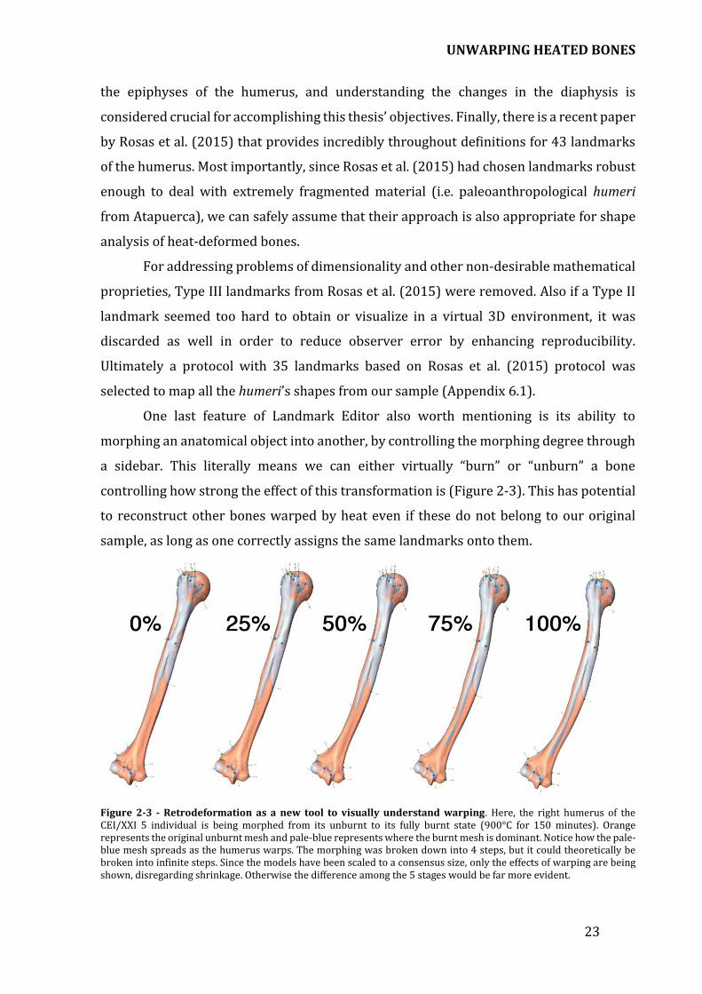
One last feature of Landmark Editor also worth mentioning is its ability to
morphing an anatomical object into another, by controlling the morphing degree through
a sidebar. This literally means we can either virtually “burn” or “unburn” a bone
controlling how strong the effect of this transformation is (Figure 2-3). This has potential
to reconstruct other bones warped by heat even if these do not belong to our original
sample, as long as one correctly assigns the same landmarks onto them.
Figure 2-3 - Retrodeformation as a new tool to visually understand warping. Here, the right humerus of the CEI/XXI 5 individual is being morphed from its unburnt to its fully burnt state (900°C for 150 minutes). Orange represents the original unburnt mesh and pale-blue represents where the burnt mesh is dominant. Notice how the pale-blue mesh spreads as the humerus warps. The morphing was broken down into 4 steps, but it could theoretically be broken into infinite steps. Since the models have been scaled to a consensus size, only the effects of warping are being shown, disregarding shrinkage. Otherwise the difference among the 5 stages would be far more evident.

Materials and Methods
24
2.5 GEOMORPH: INTEGRATING GEOMETRIC MORPHOMETRICS IN R
After obtaining the landmark configurations for our dataset with the help of
Landmark Editor, these are ready for being statistically analyzed. In R, the geomorph
package allows the execution of the full workflow of GMM, even though we jumped the
first step by doing it in Landmark Editor (an external software, easier to use for this
particular part). The full workflow of GMM can be summarized as:
1. Data collection (i.e. landmark digitizing);
2. Data input (i.e. bringing landmark data into R);
3. Data manipulation (i.e. estimating missing values);
4. Generalized Procrustes Analysis (Gower, 1975; Rohlf & Slice, 1990);
5. Data exploration and visualization (Klingenberg, 2013);
6. Data analysis (Mitteroecker & Gunz, 2009).
The two last steps include all the standard techniques of the Geometric
Morphometrics toolkit, including Principal Component Analysis (Mitteroecker &
Bookstein, 2011), Canonical Variates Analysis (Campbell & Atchley, 1981), Partial Least-
Squares (Rohlf & Corti, 2000; Bookstein et al., 2003), Multivariate Regression and
Procrustes ANOVA (Zelditch et al., 2012; Adams et al., 2013), Thin-Plate Spline
Interpolation (Bookstein, 1989; Green, 1996), among others. For more details on the
abilities of the geomorph, check Adams & Otárola-Castillo (2013) and Adams et al. (2015)
The above-mentioned methods allow us to perform statistical analysis of shape
variation and its covariation with other variables (Bookstein, 1997a). Moreover, Thin-
Plate Spline (TPS) is particularly important, since it can be used to deform a
tridimensional shape into another (Gunz & Mitteroecker, 2013). Therefore it has
implications for Objective no. 2.b: to reconstruct the original bone shape, before the heat-
induced changes have occurred. However it should be noted that the way in which
Landmark Editor does this is even easier, and allows partially morphed shapes to be
created and saved (thus 3D printable), as well as it has been show previously in Figure
2-3.

UNWARPING HEATED BONES
25
2.6 PROCRUSTES SUPERIMPOSITION
“Shape is all the geometrical information that remains when location, scale and
rotational effects are filtered out from an object.”
— (Dryden & Mardia, 1998: 1)
Applying Procrustes’ algorithms is the contemporary way to obtain insights into
morphology and extracting shape information (Rohlf & Slice, 1990; Goodall, 1991; Dryden
& Mardia, 1998; Zelditch et al., 2012). This approach is of such ubiquity in Geometric
Morphometrics that in a recent review of the state-of-the-art, Adams et al. (2013) dubbed
contemporary approaches to statistical analysis of shape as the “Procrustes Paradigm”.
Generalized Procrustes Analysis (GPA) was first introduced by Gower (1975) as a
functional algorithm for removing the effect of position, rotation and size in a set of
multiple individuals represented by Cartesian coordinates (Figure 2-4). By discarding this
information we obtain a set of consensus shapes in which each is at the orientation,
location and scale that minimizes its distance from the reference while maintaining its
key geometric proprieties in what is called the Kendall’s shape space (Kendall, 1977;
Small, 1996; Kendall et al., 2009). This is the essential algorithmic step preceding data
analysis within the realm of GMM. After this algebraic procedure, most tools from
multivariate statistics become applicable to any dataset of landmark multidimensional
arrays (Zelditch et al., 2012; Benítez & Püschel, 2014).
Figure 2-4 - Illustration of Procrustes Superimposition with the CEI/XXI 26 individual. Dark colored humerus represents the unburnt mesh and the lighter is the same bone after the heating experiment (900°C for 195 minutes). The GPA can be broken into 3 steps: A) translation, B) rotation and C) scaling. After A, B, C are performed, Procrustes Superimposition is achieved among the anatomical structures, meaning consensual shapes in Kendall’s space were obtained and thus, these bones are ready for shape analysis.

Materials and Methods
26
There are two very important scalar vectors obtained from bringing our
morphologies into the Kendall’s shape space that seem to have practical correspondence
to two critical concepts from burnt remains theory. The already mentioned Full
Procrustes Distances (DF) and differences in Centroid Size (CS) as independent
quantitative measurements of heat-induced skeletal warping and shrinking, respectively.
It should be noted that there are no references in the literature, previous to the
publication of this manuscript, of a geometrically definable quantitative analysis of these
two phenomena. Which together with fractures and color alterations represent the main
spectrum of heat-induced skeletal changes (Gonçalves et al., 2014).
A simpler and older version of GPA is Ordinary Procrustes Analysis (OPA). Instead
of performing a Procrustes superimposition for a whole sample, it is only applicable to 2
individuals. The mathematical steps for performing an OPA were actually laid down by
renowned anthropologist Franz Boas (1905), for addressing shortcomings of using
standard anatomical positioning (e.g. Frankfurt orientation). Later, it was reformulated
for allowing matrix algebra calculations, to answer questions in psychometry (Mosier,
1939). Only with Gower (1975) does OPA gets generalized enough to allow infinite
sample size, thus becoming known as GPA. Afterwards, much of the theoretical work that
consolidated Procrustes superimposition as an elegant and mathematically coherent
method of statistical shape theory is due to David Kendall (1984, 1985, 1989), who was
initially motivated to apply superimposition algorithms in order to study shape and form
characteristics of different megalithic sites (Broadbent, 1980; Kendall & Kendall, 1980).
For our purposes of addressing specific problems in burnt osteology, which
includes estimating quantitatively warping and shrinking, we could either do OPA for
every pair of unburt-and-burnt individual bone, or do a GPA for the whole sample. The
second approach was preferred because it is far faster and easier to implement nowadays,
and also because it gives us far more data. Since GPA is performed to the whole sample, it
is possible to calculate all possible Full Procrustes distances among our 38 geometric
individuals in the sample (i.e. a total of 384 Procrustes distances), even though only 19 of
these are relevant to directly estimate warping. However, OPA is still a crucial concept for
this thesis, in the sense that it is the only methodological way for others to test (with their
own data) the predictive abilities of the statistical models that have been designed. Which
are shown later in Chapter 3.7.

UNWARPING HEATED BONES
27
2.7 THIN-PLATE SPLINE INTERPOLATION
Grid plotting via interpolate functions had its roots in a simple, yet powerful idea
of using deformation grids as a way for illustrating and formalize shape differences among
geometrical entities. This intuition dates back to the 1528 manuscript by Albrecht Dürer
on the variation of human proportions (Figure 2-5).
Figure 2-5 - A few examples of the first known use of deformation grids in anatomy. Vectorial graphics presented here were redrawn after Dürer’s ([1528] 1969) original drawings.
Later in 1917, D’Arcy Thompson revisited the idea with what he called ‘Cartesian
transformations’. His insight was to not only use this tool for describing biological
variability but also to apply it for interspecific form comparison (Figure 2-6). Yet
Thompson ([1917] 1992) had also hand-drawn his grids, so these are actually also pre-
Cartesian and error-prone. The one to solve this problem was Bookstein (1989), by
implementing an interpolant function commonly used to address problems in material
physics. With a TPS algorithm it is possible to computationally define a deformation grid
from two sets of Cartesian coordinates. Thus effectively mapping the differences in form
between two anatomical entities.
Figure 2-6 - Cartesian transformations from Homo sapiens into Pan troglodytes and a Papio sp. vectorial graphics adapted from Thompson’s ([1917] 1992) classic On Growth and Form.
Materials and Methods
28
As a methodology TPS Interpolation serves 3 main goals in statistical shape
analysis: (1) as it primary purpose it uses deformation grids as visualization tools of shape
modification (Mitteroecker & Bookstein, 2011; Klingenberg, 2013); (2) it is used as well
in dimensionality reduction, in the case of 3D data specifically from 3k degrees of freedom
into 3k-7 with no loss of information. Obtaining the correct degrees of freedom allows the
use of conventional statistical tests without having worries concerning complicated
mathematical details (Zelditch et al., 2012); (3) additionally, it enables superimposition
(sliding) of semilandmarks (Gunz & Mitteroecker, 2013).
For this thesis’ objectives, the first point is perhaps the most crucial. But even if
one was not concerned with graphical displays, TPS is useful since it performs an
eigenanalysis of the bending energy matrix thus obtaining a parsimonious matrix that
describes shape differences between a reference and another shape through partial
warps scores, which can be directly used (unlike coordinates from GPA) for conventional
statistical analysis, such as regression.
2.8 LOGISTIC MODEL TREES: A CLASSIFICATION ALGORITHM
The chosen Machine Learning algorithm to create our predictive models was
Logistic Model Trees (LMT). It combines the heuristics of Logistic Regression and
Decision Trees during its supervised training process. This is quite useful, since the
former tends to show low variance, but high bias. While the later usually has low bias, but
is less stable and prone to overfitting (Landwehr et al., 2005). In a recent preliminary
study dealing also with a classification problem, LMT beat in overall accuracy many other
state-of-the-art Machine Learning algorithms when trying to estimate sex from
Procrustes-aligned shape matrices (Coelho et al., 2015).
For our dataset LMT is optimal, since the data we collected already has a bias and
variance problem. Thus a classification algorithm that is robust to both problems is the
most scientifically honest and sound approach. As a structured predictive model, it
consists of a standard decision tree construction with logistic regression functions at its
leaves (Figure 2-7). This makes it harder to interpret than simpler classification

UNWARPING HEATED BONES
29
algorithms, since it cannot be graphically represented as a tree of decisions neither as an
elegant regression-style formula.
However, readers can still easily use any models created with LMT through loading
their own landmark configurations into R and force an OPA between their obtained
landmarks and our reference average shape, and then analyze their data by running the
code provided in the following chapters.
LMT(examples){ root <- new Node() alpha <- getCARTAlpha(examples) root.buildTree(examples, null) root.CARTprune(alpha) } buildTree(examples, inititalLinearModels){ numIterations = CV_Iterations(examples, inititalLinearModels) initLogitBoost(initialLinearModels) linearModels <- copyOf(inititalLinearModels) for i = 1...numIterations{ logitBoostIteration(linearModels, examples) } split <- findSplit(examples) localExamples <- split.splitExamples(examples) sons <- new Nodes[split.numSubsets()] for s = 1...sons.length{ sons.buildTrees(localExamples[s], nodeModels) } } CV_Iterations(examples, initialModels) { for fold = 1...5 { initLogitBoost(inititalLinearModels) # split into training/test sets train <- trainCV(fold) test <- testCV(fold) linearModels <- copyOf(inititalLinearModels) for i = 1...200{ logitBoostIteration(linearModels, train) logErros[i] += error(test) } } numIterations = findBestIteration(logErrrors) return numIterations }
Figure 2-7 - Pseudocode for implementing Logistic Model Trees, (adapted from Landwehr et al., 2005)

Materials and Methods
30

UNWARPING HEATED BONES
31
3 RESULTS AND DISCUSSION
3.1 GETTING STARTED
All the results presented within this manuscript have been automatically
generated as a .docx file through the knitr package for R. Even this paragraph itself was
not written in Word, but instead in R. Contrary to the standard, this has the advantage of
creating a text accompanied by the exact code that generated the graphics, tables and
other results. Hence, increasing the reproducibility criteria, allowing other researchers to
easily run the data analysis into their personal computers as long as they have data for it.
This adheres to the tenants of the Open Data movement and Science 2.0 philosophy by
promoting data analysis transparency among scientists.
If you desire to execute in your computer the whole data analysis present in this
thesis you should first make sure to:
Have installed R and the latest version of RStudio
Install the latest version of the knitr package, by writing
install.packages("knitr") in your RStudio console.
To run the code that produced my thesis output:
Open RStudio, and go to File > New > R Markdown
Paste in the contents of the results.Rmd available in this thesis’ online repository
http://git.io/vYjNa, or by contacting me: [email protected]
Click Knit Word
You should not forget to use setwd("YOUR/FOLDER/LOCATION") to where the
landmark files and 3D meshes are located. Or even easier, just open the HOTProject-
GM.Rproj file, since it automatically loads everything.

Results and Discussion
32
It should run fine as long as you follow what is said above. Just to clarify, from here
on, every time you see chunks of code, you can easily identify them through the box with
light background and different font type that gets colored by association of the type of
programming object. There you also see some commands that usually have a # symbol
followed by some sentence, which are explanatory commentaries upon what the code is
doing to help non-experts understanding what is being programmed. If it is a double ##
it is an output generated by the code.
3.2 DATA INPUT
Our landmarks were obtained from the free software Landmark Editor. Likewise,
it was attempted to use auto3Dgm for the same aim, and also in order to compare the two
approaches (i.e. manual versus automatic). Nonetheless, as it can be seen in Figure 3-1
that was generated from the output of the auto3Dgm algorithm, a total of 5 burnt bones
were inadequately aligned. Regrettably, this would effectively reduce the geometric n by
10, since their counterparts (i.e. the unburnt) would not be used for any particular
purpose without their pair. Considering that no way was found within R to solve this
problem, this approach was discontinued mid-way during the project because it would
considerably reduce our n.
Figure 3-1 - Shapes automatically scaled and aligned by auto3Dgm using 256 pseudolandmarks. The incorrectly aligned bones are presented in red, which are all burnt humeri (of CEI/XXI 5, 32, 35, 51 and 65). Notice that some have been mirrored (turned into left antimeres), others were rotated 180 degrees in an axis and one was rotated in another axis and mirrored, overall very chaotic algebraic transformations. Despite hundreds of attempts, no elegant solution for this problem was found, and the use of auto3Dgm for this project was abandoned.

UNWARPING HEATED BONES
33
SW <- read.csv(file = './data/SingularWarps.csv', header = TRUE) # loads all the variables that aren't shape-data. rawdata <- pts2array(pts.dir = './data/pts-files') # loads raw landmark data into R, similary to readland.nts(), check ?readland.nts dimnames(rawdata)[[3]] # reads each geometric configuration’s name. Useful to confirm if the order and naming are correct and consistent with singular warps order. Codenames have ID, sex and burning temperature.
## [1] "CEIXXI05F" "CEIXXI05F900" "CEIXXI08F" "CEIXXI08F700" ## [5] "CEIXXI17M" "CEIXXI17M900" "CEIXXI24F" "CEIXXI24F800" ## [9] "CEIXXI26F" "CEIXXI26F900" "CEIXXI29M" "CEIXXI29M800" ## [13] "CEIXXI32F" "CEIXXI32F800" "CEIXXI35M" "CEIXXI35M900" ## [17] "CEIXXI43M" "CEIXXI43M800" "CEIXXI49F" "CEIXXI49F850" ## [21] "CEIXXI50F" "CEIXXI50F900" "CEIXXI51M" "CEIXXI51M900" ## [25] "CEIXXI53F" "CEIXXI53F800" "CEIXXI57M" "CEIXXI57M900" ## [29] "CEIXXI64M" "CEIXXI64M800" "CEIXXI65F" "CEIXXI65F900" ## [33] "CEIXXI79M" "CEIXXI79M900" "CEIXXI86M" "CEIXXI86M1000" ## [37] "CEIXXI97F" "CEIXXI97F1050"
3.3 DATA PRE-PROCESSING AND GPA
As result of poor preservation some humeri from our sample do not have
anatomical parts where specific landmarks should be located. This was either due to
taphonomic processes or because of the heating experiment itself. However, robust
methods have been devised within statistical shape analysis in order to handle missing
data. For solving this, the very convenient estimate.missing() function from the
geomorph package is used to generate estimates of the missing landmarks.
EM <- estimate.missing(rawdata, method = 'TPS') # This command estimates missing landmarks using either Thin Plate Spline or Regression. Here TPS was chosen.
Preforming GPA over your data is the quintessential step to start a statistical shape
analysis. In geomorph this is achieved with the gpagen() command. Our aligned
Procrustes coordinates, and specimens' centroid sizes are recorded as the variables
procrustes$coords and procrustes$Csize, respectively.

Results and Discussion
34
procrustes <- gpagen(EM, ShowPlot = FALSE) # Procrustes superimposition, creates a viable dataset for applying geometric morphometrics methods.
Right now we have everything we need to start a multivariate statistical analysis
of shape and its covariation with other variables (Bookstein, 1997a). However it is better
to do some graphical exploration, in order to understand our data and correctly obtain
fruitful inferences from it.
3.4 EXPLORATORY DATA ANALYSIS
An essential step of every data analysis that rarely takes the spotlight is the visual
data exploration that antecedes inference or modeling. It is extremely important in the
sense that allows us to allocate our precious time in more fruitful avenues, rather than
trying everything for all the variables without a rigorous aim in mind.
The exploratory data analysis was broken into two main steps. First we intended
to summarize, describe and visualize general aspects of our data. This was achieved in
Table 1 and Figure 3-2, but also complemented with the Table 4 in Appendix 6.4. Second,
we used a method based on the Geometric Morphometrics toolkit to look for possible
errors in the landmark placing protocol.
3.4.1 DESCRIPTIVE STATISTICS
Now, we perform quick and very simple data manipulation to allow the
construction of graphical plots and tables. We provide counts of values, and many classic
measures developed by the theory of probability distributions.
logSize <- log(as.numeric(procrustes$Csize)) # The log of Centroid Size is useful and recommended in the literature for creating models.
Shapes <- procrustes$coords # Gives a new name easier to remember. kable(stat.desc(cbind(logSize, SW[,-c(1:4)]), norm = TRUE), digits = 2) # Creates a table. Categorical variables were removed because most of these stats only make sense for numeric variables.

UNWARPING HEATED BONES
35
Table 1 - Descriptive statistics for the vectors of numeric variables in our dataset.
logSize months.buried age temperature duration mass
n of values 38.00 32.00 38.00 38.00 38.00 38.00
n of nulls 0.00 0.00 0.00 19.00 19.00 0.00
n of NA 0.00 6.00 0.00 0.00 0.00 0.00
min 6.35 71.00 70.00 0.00 0.00 23.20
max 6.69 84.00 90.00 1050.00 195.00 124.49
range 0.34 13.00 20.00 1050.00 195.00 101.29
sum 249.39 2358.00 3050.00 16500.00 2569.00 2588.03
median 6.59 73.00 81.00 350.00 37.50 62.16
mean 6.56 73.69 80.26 434.21 67.61 68.11
SE 0.01 0.52 1.02 71.96 11.64 4.44
CI95 0.03 1.06 2.08 145.80 23.59 9.00
variance 0.01 8.61 39.87 196770.98 5151.98 750.38
SD 0.09 2.93 6.31 443.59 71.78 27.39
var.coef 0.01 0.04 0.08 1.02 1.06 0.40
g1 -0.54 2.64 -0.11 0.05 0.26 0.33
SC-g1 -0.70 3.19 -0.14 0.06 0.34 0.43
g2 -0.65 6.63 -1.31 -1.99 -1.66 -1.01
SC-g2 -0.43 4.10 -0.88 -1.33 -1.11 -0.67
W 0.95 0.60 0.94 0.71 0.78 0.94
W’s p-value
0.08 0.00 0.04 0.00 0.00 0.06
Legend: SE = Standard Error of the Mean; CI95 = Confidence Intervals of the Mean at 95%; SD = Standard Deviation; var.coef = variation coefficient; g1 = the skewness coefficient; SC-g1 = significant criterium of g1, if > 1 then skewness is significantly different than zero; g2 = kurtosis coefficient; SC-g2 = same definition as g1SC but for kurtosis; W = the statistic of a Shapiro-Wilk test of normality; W’s p-value is the associated probability of the W statistic.
Next, we check potential correlations and possibility for regression models in our
non-shape related data (i.e. Singular Warps) and the logarithm of Centroid Size. This last
measure is also included because it is a vector of size and can be easily represented.
Procrustes landmarks are a p * k * x data matrix, in our case, a shape configuration of 35
landmarks, 3 dimensions and 38 individuals. Therefore, it would be too complicated to
visualize through the graphical device of Figure 3-2 or Table 1 and so shape data was not
included here.

Results and Discussion
36
scatterplotMatrix(cbind(logSize, SW[ ,-c(1,2)]), col = c('#f1c40f', '#e74c3c', 'black'), lwd = 2)
Figure 3-2 - Scatterplot matrix of our variables to visually complement the descriptive statistics of Table 1. Yellow lines are simple linear models (lm) while red lines are generalized additive models (GAM) with respective 95% confidence intervals in dashed red lines.
3.4.2 EXPLORATION OF UNCERTAINTY
Since we have seen how all the other variables are interacting, now we focus solely
on our shape data. First, we try to see if there are any outliers in terms of landmark
configurations within our dataset. This can be done with the plotOutliers() function,
which is very useful because it allows researchers to verify if any specimen was
incorrectly digitized (e.g. landmarks out of order or anatomically misplaced).
outliers <- plotOutliers(Shapes) # Plots potential outliers through calculation of Procrustes Distance.

UNWARPING HEATED BONES
37
Figure 3-3 - Plot for potential shape outliers. After GPA, all 38 shapes in the sample were plotted, through Procrustes distances from Mean Shape. The burnt state of 4 different humeri deviate considerably from the average shape and so we could be looking at potentially outliers in our sample.
Interestingly, after a visual check in Landmark Editor, none of the “outliers”
marked in red (Figure 3-3) had actually misplaced or disordered anatomical landmarks.
These 4 appear as outliers because of how much heat-induced warping and fracturing
affected their shape. Together, CEI/XXI 65, 32, 5, and 50 represent the most extremely
modified-by-heat humeri within our sample. This can be confirmed visually with the 3D
meshes files, but is also sustained by performing a PCA on our data.
3.5 PRINCIPAL COMPONENTS ANALYSIS
The following function plots a set of Procrustes-aligned specimens in tangent
space along their principal axes (Figure 3-4). In our case the plot illustrated that all the
bones before heating, and also the bones that were not much affected by the heating
experiment tend to cluster around the Origin of the Cartesian plot of the two Principal
Components. The more extremely modified by heat are dispersed in the periphery in what
seems to be pseudorandom directions. A bigger dataset is needed to understand the
patterns governing these directions, which are possibly describing different ways in
which the bone is being deformed by heat.
# Define graphical proprieties of the PC plot: gp <- as.factor(SW$temperature) col.gp <- c('#bdc3c7', '#f1c40f', '#f39c12', '#e67e22', '#d35400', '#e74c3c', '#c0392b') # Picking html colors for the plot pch.gp <- c(12:18)

Results and Discussion
38
names(col.gp) <- levels(gp) names(pch.gp) <- levels(gp) col <- col.gp[match(gp, names(col.gp))] pch <- pch.gp[match(gp, names(pch.gp))] # Calculate a PCA: y <- two.d.array(Shapes) pc.res <- prcomp(y) pcdata <- pc.res$x # Code our plot: plot(pcdata[, 1], pcdata[, 2], pch = pch, asp = 1, col = col, cex = 1.5, xlab = paste('PC ', 1), ylab = paste('PC ', 2)) segments(min(pcdata[, 1]), 0, max(pcdata[, 1]), 0, lty = 2, lwd = 1) segments(0, min(pcdata[, 2]), 0, max(pcdata[, 2]), lty = 2, lwd = 1) text(pcdata[, 1], pcdata[, 2], dimnames(rawdata)[[3]], adj = c(-0.05, -0.7), cex = 0.7) # Add a legend: legend(0.12, 0.04, legend = levels(gp), pch = pch.gp, col = col.gp)
Figure 3-4 - Dataset projected onto PC1-2 Subspace. Together PC1+PC2 have a Cumulative Proportion of Variance = 0.4490, meaning they explain nearly half of the variance in our sample. The 0 value in temperature is actually a NULL value corresponding to the geometries of the unburnt counterparts.
One should never forget that ultimately, PCA is nothing more than a rotation of the
original data. Its usefulness lies in the fact that our features will exhibit covariances

UNWARPING HEATED BONES
39
because they are influenced by and interact with common processes. The magnitudes of
variances described by all components can be seen in Figure 3-5.
# To plot a graph of the proportion of variance explained by each PC: pvar <- (pc.res$sdev^2)/(sum(pc.res$sdev^2))
names(pvar) <- seq(1:length(pvar))
barplot(pvar, main = 'Eigenvalues', xlab= 'Principal Components', ylab = '% Variance', col = 'black', las = 2, cex.names = 1)
Figure 3-5 - Scree plot of the proportion of variance in descending order. The cumulative proportion of the first 13 PCs explain more than 90% of the variance in the shapes sample.
3.6 THIN-PLATE SPLINE PLOTS
Also important is to visualize the changes within a particular bone, between its
pre-heating shape and deformed-by-heat shape through TPS (Figure 3-6). For achieving
this, we generated thin-plate spline deformation grids. To visualize 3D data deformations
into the paper format that bounds this thesis, thin-plate spline grids are show in the x-y
and x-z axis (Figure 3-7). The y-z axis is not presented, because it is very difficult to
understand anything from that perspective. Also, because the other two views in 2D are
sufficient to show all the 3 axes from 3D already. Thus, a third view is redundant.
GP <- gridPar(pt.bg = 'black', pt.size = 0.5, n.col.cell = 25) # Defines general graphical proprieties of the following plots.

Results and Discussion
40
plotRefToTarget(Shapes[,,1], Shapes[,,2], gridPars = GP, method = 'TPS') # TPS plot of CEIXXI05F
Figure 3-6 - TPS plot of individual CEI/XXI 5, with reference shape being the pre-heating state and deforming shape the post-heating shape. As it can be seen, even though there are only 4 landmarks in the diaphysis, these were enough to visually demonstrate the bending curvature resulting from the heat-induced skeletal warping which is most notable in the X-Y axes.
plotRefToTarget(Shapes[,,13], Shapes[,,14], gridPars = GP, method = 'TPS') # TPS plot of CEIXXI32F
Figure 3-7 - TPS plot of individual CEI/XXI 32, with reference shape being the pre-heating state and deforming shape the post-heating shape. As it can be seen this bone has suffered considerable from the effects of heat-induced skeletal shrinking. Another interesting feature of individual 32 was that it fractured nearly the middle, what caused warping to create a rotational or torsion effect in the distal part of the humerus, this can be understood easily by looking at the left side of the Y-Z perspective.
Only individual CEI/XXI 5 and 32 are shown here in the results for illustrative
purposes because having the whole dataset would take too much space. For more
comprehensive results check the Appendix 6.6. There, a total of 19 TPS deformation plots
can be found, fully describing the whole dataset.
3.7 PREDICTIVE MODELLING
“Essentially, all models are wrong, but some are useful.”
— (George Box in Box & Draper, 1987: 424)
Creating models with such reduced sample sizes is usually not a good decision.
Here, we create them, to show how easy it is to implement and test predictive models with
our kind of data. While all models presented are already fully operational, it is hard to
truly estimate their actual degree of accuracy. This is due to deficient implementation of
cross-validation algorithms when dealing with badly represented factors and small n.

UNWARPING HEATED BONES
41
3.7.1 PROCRUSTES ANALYSES OF VARIANCE
A Procrustes ANOVA is used to quantify the relative amount of shape variation
attributable to one or more variables in a linear model and assesses this variation through
permutation. In geomorph the function procD.lm() allow us to input data by a y~X
formula, where 'y' specifies the response variable (shape data), and 'X' contains one or
more independent variables (Adams et al., 2015).
procD.lm() follows the philosophy that:
Randomization procedures are used to generate empirical sampling distributions
to assess significance of effects.
Effect sizes are estimated as standard deviates from such sampling distributions.
The function performs statistical assessment of the terms in the model using
Procrustes distances among specimens, instead of explained covariance matrices among
variables. With this approach, the sum-of-squared Procrustes distances are used as a
measure of SS and permutation is used to evaluate observed SS (Adams & Otárola-Castillo,
2013).
# The residual SS (RSS) of a linear model (also called the sum of squared error, SSE) is found as follows: RSS <- function(fit) sum(diag(resid(fit)%*%t(resid(fit)))) Sex <- SW$sex fit1 <- lm(y ~ 1) # model contaning just an intercept fit2 <- lm(y ~ logSize) # allometric scaling of shape fit3 <- lm(y ~ logSize + Sex) # previous model + sexual dimorphism fit4 <- lm(y ~ logSize * Sex) # previous model + interaction between sex and log(CS) # For any model 'fit', we can summarize the error of prediction by calculating RSS.
RSS(fit1)
## [1] 0.06791796
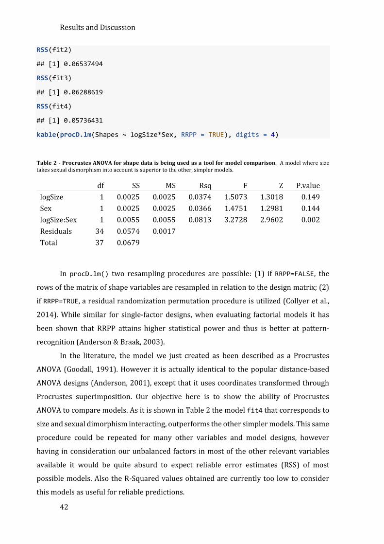
Results and Discussion
42
RSS(fit2)
## [1] 0.06537494
RSS(fit3)
## [1] 0.06288619
RSS(fit4)
## [1] 0.05736431
kable(procD.lm(Shapes ~ logSize*Sex, RRPP = TRUE), digits = 4)
Table 2 - Procrustes ANOVA for shape data is being used as a tool for model comparison. A model where size takes sexual dismorphism into account is superior to the other, simpler models.
df SS MS Rsq F Z P.value
logSize 1 0.0025 0.0025 0.0374 1.5073 1.3018 0.149
Sex 1 0.0025 0.0025 0.0366 1.4751 1.2981 0.144
logSize:Sex 1 0.0055 0.0055 0.0813 3.2728 2.9602 0.002
Residuals 34 0.0574 0.0017
Total 37 0.0679
In procD.lm() two resampling procedures are possible: (1) if RRPP=FALSE, the
rows of the matrix of shape variables are resampled in relation to the design matrix; (2)
if RRPP=TRUE, a residual randomization permutation procedure is utilized (Collyer et al.,
2014). While similar for single-factor designs, when evaluating factorial models it has
been shown that RRPP attains higher statistical power and thus is better at pattern-
recognition (Anderson & Braak, 2003).
In the literature, the model we just created as been described as a Procrustes
ANOVA (Goodall, 1991). However it is actually identical to the popular distance-based
ANOVA designs (Anderson, 2001), except that it uses coordinates transformed through
Procrustes superimposition. Our objective here is to show the ability of Procrustes
ANOVA to compare models. As it is shown in Table 2 the model fit4 that corresponds to
size and sexual dimorphism interacting, outperforms the other simpler models. This same
procedure could be repeated for many other variables and model designs, however
having in consideration our unbalanced factors in most of the other relevant variables
available it would be quite absurd to expect reliable error estimates (RSS) of most
possible models. Also the R-Squared values obtained are currently too low to consider
this models as useful for reliable predictions.

UNWARPING HEATED BONES
43
3.7.2 GROWING TREES INTO ANSWERS
The following model lmtFit1 uses Logistic Model Trees (Landwehr et al., 2005) to
predict if a humerus was burnt or not with 92.1% accuracy, by being trained on the first
8 Principal Components of our sample. So how should nonmorphometricians interested
in burnt remains proceed to apply this model to a humerus from their own sample? By
following the whole protocol: (1) 3D Scanning a humerus; (2) Processing it in MeshLab;
(3) Obtain the defined 35 Landmarks for that bone; (4) Perform an OPA on the obtained
configuration by using the mean shape of our sample as the reference shape; (5) perform
a PCA on the configuration, (6) apply the model by using the R function predict() on his
first 8 PCs. Alternatively, step 1, 2, and 3 could be substituted by obtaining landmarks
directly from a MicroScribe or a similar device.
data.models <- cbind(SW[,-c(1, 2)], logSize, pcdata[ ,1:8]) lmtFit1 <- LMT(burnt ~ PC1+PC2+PC3+PC4+PC5+PC6+PC7+PC8, data = data.models) summary(lmtFit1)
## ## === Summary === ## ## Correctly Classified Instances 35 92.1053 % ## Incorrectly Classified Instances 3 7.8947 % ## Kappa statistic 0.8421 ## Mean absolute error 0.2245 ## Root mean squared error 0.297 ## Relative absolute error 44.8947 % ## Root relative squared error 59.4075 % ## Coverage of cases (0.95 level) 100 % ## Mean rel. region size (0.95 level) 97.3684 % ## Total Number of Instances 38 ## ## === Confusion Matrix === ## ## a b <-- classified as burnt ## 18 1 | a = no ## 2 17 | b = yes
However, in most cases, for the trained osteologist it is easy to understand if a bone
was burnt or not by just looking at it. Even if dealing with particularly complicated cases,
there are already well established methods like Fourier Transform Infrared Spectroscopy
(Munro et al., 2007; Thompson et al., 2009) or histological techniques that can erase most

Results and Discussion
44
doubts if they arise (Bradtmiller & Buikstra, 1984; Nelson, 1992; Hiller et al., 2003). So
why would a model like this be useful? It would not: it is too time consuming. A far more
useful model would be a similar one that could not only determine if a bone was burnt but
at which maximum temperature it was burnt. Next, we implement such model in a similar
fashion.
lmtFit2 <- LMT(as.factor(temperature) ~ PC1+PC2+PC3+PC4+PC5+PC6+PC7+PC8, data = data.models) summary(lmtFit2)
## ## === Summary === ## ## Correctly Classified Instances 32 84.2105 % ## Incorrectly Classified Instances 6 15.7895 % ## Kappa statistic 0.7415 ## Mean absolute error 0.1091 ## Root mean squared error 0.2116 ## Relative absolute error 54.8523 % ## Root relative squared error 68.3659 % ## Coverage of cases (0.95 level) 100 % ## Mean rel. region size (0.95 level) 56.391 % ## Total Number of Instances 38 ## ## === Confusion Matrix === ## ## a b c d e f g <-- classified as ## 19 0 0 0 0 0 0 | a = 0 ## 0 1 0 0 0 0 0 | b = 700 ## 4 0 2 0 0 0 0 | c = 800 ## 0 0 0 1 0 0 0 | d = 850 ## 1 0 0 0 8 0 0 | e = 900 ## 1 0 0 0 0 0 0 | f = 1000 ## 0 0 0 0 0 0 1 | g = 1050
Despite the lack of values for each factor, plus the short range of maximum
temperatures experimented with, which of course causes overfitting. Combined with the
low diversity of the factors themselves, which forces us to use a classification algorithm
for temperatures instead of a regression, our model lmfit2 provided what seems to be
very promising results (Overall Accuracy = 84.21%). Here is shown a stepping-stone from
where one could eventually create a very powerful model by increase n in each of the
factors of the dependent variable, in order to reduce overfitting while increasing or
maintaining overall accuracy.

UNWARPING HEATED BONES
45
4 CONCLUSION
“All anthropological analyses conducted on burned remains will be wholly and
fundamentally inaccurate”
— (Thompson, 2005: 6)
As a project aimed at improving the current methods in burnt remains theory, it is
still in a long way from bringing any effective impact to the field. Sample size was a major
problem that led most of the data analysis towards a theoretical cul-de-sac. Low sample
size undermines reliability, reduces statistical power and reproducibility of results, while
overestimating effect size (Stodden, 2015). It is therefore a problem that can only be
overcome by keeping on collecting data, with a focus on well-balanced experimental
design. Meaning that the factors within variables must not be so disproportionately
represented as they actually are. For example: up to now, 9 skeletons were burnt at 900°C,
other 6 at 800°C, and for all the other temperatures experimented with (500, 700, 850,
1000 and 1050°C) we have only one case representing each. Obviously this severely limits
the predictive power of any model since you cannot train a machine-learning algorithm
with only a few cases for each factor. Certainly there is no algorithm that will learn how
to represent these in such conditions. In spite of that, many experimental studies in the
burnt osteology literature have even smaller samples. There are the typical n = 1 studies
(e.g. DeHaan & Nurbakhsh, 2001) that usually are about burning a carcass of an animal to
record the effects. Others, such as Thurman and Willmore (1981) had burned 8 human
humeri for their analysis; and Nugent (2010) attempted to estimate the biological profile
of 19 cremated individuals, yet only 18 humeri were analyzed. Contrasting, our sample
will keep on growing into the future, benefiting from being part of the HOT Project and
the CEI/XXI. But again: the solution is to focus on good experimental design, just
increasing n blindly will not be enough.
Unfortunately, my data analysis is also included in a project suffering from the
‘myth of flesh’, which shows an overall high prevalence in anthropological studies
concerning taphonomy. It has been explained as a “(…) bias [that] manifests itself in
experimental research and analyses that treat skeletal elements as though they had
always existed without the encumbrances of skin, muscle, ligament and other soft tissues

Conclusion
46
(…)” (Haglund & Sorg, 1996: 3). Eventually, even if a reasonable sample size is reached in
the future and powerful predictive models are created, one must first question: to what
point would these be reliable when applied to burnt bones originating from forensic
cases? Prudency is mandatory, since forceful generalization of specific models usually
leads to worthless results. Current hypothesis state that soft tissues are not just
restricting heat transfer differentially through their thickness and composition, but also
cutting off the oxygen supply to the underlying bone (McKinley & Tech, 2015). This leads
us to another problem: actual combustion versus just heat transfer.
Even though terms such as ‘burning’, ‘burned’ or ‘burnt’ have been used
recurrently throughout this thesis, it is explicit that the experiment only deals with
thermally modified bones, which were not actually burned amid fire. Consequently, other
variables that are not being accounted for, that can also bias any predictions to real-life
situations, are the type and quantity of fuel, plus oxygen content or supply. Such variables
are of the uttermost importance when dealing with combustion (i.e. fire), but do not really
interfere with heat-transfer in the absence of combustion. Thus, it would be senseless for
us to account for these, even though such variables are possibly very pertinent in arsons,
mass disasters, various ethno-historic or archaeological types of cremation, and so on
(DeHaan, 2015).
Until now, the reader might believe that no remarkable positive conclusions can
be achieved in this particular line of research. But by using a metaphor that would work
much better if a particularly famous movie title was written backwards: we just passed
through the Ugly and the Bad. So, now comes the Good.
Is thermally modified dry bone that different from typical human burnt remains?
Throughout the years evidences have come up, suggesting the gap between both might be
far shorter than previously thought. Until demonstrated otherwise (Buikstra & Swegle,
1989; Spennemann & Colley, 1989), most literature attributed warping as a phenomenon
exclusive of hydrated bones. Many papers (Baby, 1954; Binford, 1963; Thurman &
Willmore, 1981; Etxéberria, 1994) interpreted presence of warping as a discriminant
factor between burnings with prior tissue removal as opposed to excarnation absence.
Meaning that at least 35 years of burnt osteology up to that point, worked on unsupported
and false assumptions on one of its most basic aspects. Heating experiments under
controlled conditions are thus crucial for busting myths, creating insights, and stimulating
progress within this scientific domain (Thompson, 2005, 2009). But as have been

UNWARPING HEATED BONES
47
continuously cautioned, there are many problems that should be rigorously addressed. If
so, this kind of research might bring tremendously value for forensic anthropologist and
others dealing with human burnt remains.
It was demonstrated how to craft predictive models for estimating burning
conditions such as maximum temperature and it was discussed how to improve the ones
that have been created in the context of this thesis. If this research continues, these
models will hopefully become powerful enough to be used by other researchers without
any major obstacles. Even if such is not bound to happen with this particular research, it
might inspire other colleagues to obtain their own data and create their own models
based on the toolkit of GMM and ML algorithms. Since this was demonstrated here to be
a possible route, which still needs to be much more explored for the thermally modified
bones problematic.
Finally, it cannot be stressed enough how digital 3D preservation of anatomical
structures exposed to heat is essential and how staggering it is that it as been pretty much
dismissed, with the only exception found in literature being Imaizumi et al. (2014).
Subjecting osteological material to heat is a great source of data with potential to infer not
just correlation, but also causation. Simultaneously, without the proper protocol a
considerable amount of data gets destroyed as well during the process. Collecting
measurements such as lengths, mass and so on can be useful, but it is far from enough.
Perhaps most of the field is unaware of the analytical possibilities brought by having data
preserved in virtual 3D files. Even Imaizumi et al. (2014) used their collected CT scans
solely for the purpose of calculating volumetric differences. Which is possibly one of the
best ways to directly measure shrinkage, but offers no possibilities for warping
quantification. Awareness of GMM and the possibility of curating 3D databases must be
brought into burnt osteology, or otherwise knowledge that is clearly within grasp will
continue to escape us.
Models should be created with other bones as well, besides the humerus. Actually,
it was originally intended to use both femura and humeri, alas it was impossible. Because
after the experiment, femurs almost always collapsed on their own weight, having
fragmentation and far more extreme fractures, thus being overall more fragile (Figure
4-1). Following, the final n of femurs that could be 3D scanned before and after heating
was so small that would be insane to try to perform any analysis with the few obtained
3D meshes. However tibiae and ulnae tend to preserve well and can be 3D scanned in an
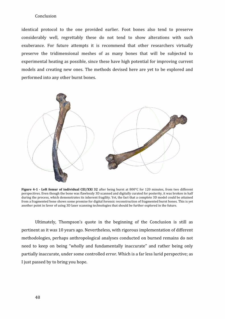
Conclusion
48
identical protocol to the one provided earlier. Foot bones also tend to preserve
considerably well, regrettably these do not tend to show alterations with such
exuberance. For future attempts it is recommend that other researchers virtually
preserve the tridimensional meshes of as many bones that will be subjected to
experimental heating as possible, since these have high potential for improving current
models and creating new ones. The methods devised here are yet to be explored and
performed into any other burnt bones.
Figure 4-1 - Left femur of individual CEI/XXI 32 after being burnt at 800°C for 120 minutes, from two different perspectives. Even though the bone was flawlessly 3D scanned and digitally curated for posterity, it was broken in half during the process, which demonstrates its inherent fragility. Yet, the fact that a complete 3D model could be attained from a fragmented bone shows some promise for digital forensic reconstruction of fragmented burnt bones. This is yet another point in favor of using 3D laser scanning technologies that should be further explored in the future.
Ultimately, Thompson’s quote in the beginning of the Conclusion is still as
pertinent as it was 10 years ago. Nevertheless, with rigorous implementation of different
methodologies, perhaps anthropological analyses conducted on burned remains do not
need to keep on being “wholly and fundamentally inaccurate” and rather being only
partially inaccurate, under some controlled error. Which is a far less lurid perspective; as
I just passed by to bring you hope.

UNWARPING HEATED BONES
49
5 BIBLIOGRAPHY
Adams, D. C.; Otárola-Castillo, E. 2013. geomorph: an r package for the collection and
analysis of geometric morphometric shape data. Methods in Ecology and Evolution.
4(4):393–399. DOI: 10.1111/2041-210X.12035.
Adams, D.; Collyer, M.; Sherratt, E. 2015. geomorph: Geometric Morphometric Analyses of
2D/3D Landmark Data. Available: http://cran.r-
project.org/web/packages/geomorph/index.html [2015, June 14].
Adams, D. C.; Rohlf, F. J.; Slice, D. E. 2013. A field comes of age: geometric morphometrics
in the 21st century. Hystrix, the Italian Journal of Mammalogy. (1). DOI:
10.4404/hystrix-24.1-6283.
Anderson, M. J. 2001. A new method for non-parametric multivariate analysis of variance.
Austral Ecology. 26(1):32–46. DOI: 10.1111/j.1442-9993.2001.01070.pp.x.
Anderson, M.; Braak, C. ter. 2003. Permutation tests for multi-factorial analysis of
variance. Journal of Statistical Computation and Simulation. 73(2):85–113. DOI:
10.1080/00949650215733.
Baby, R. S. 1954. Hopewell Cremation Practices. The Ohio Historical Society Papers in
Archaeology. 1:1–7.
Benítez, H. A.; Püschel, T. A. 2014. Modelando la Varianza de la Forma: Morfometría
Geométrica Aplicaciones en Biología Evolutiva. International Journal of Morphology.
32(3):998–1008. DOI: 10.4067/S0717-95022014000300041.
Binford, L. R. 1963. An Analysis of Cremations from Three Michigan Sites. Wisconsin
Archeologist. 44:98–110.
Boas, F. 1905. The Horizontal Plane of the Skull and the General Problem of the
Comparison of Variable Forms. Science. 21(544):862–863.

Bibliography
50
Bolitho, M.; Kazhdan, M.; Burns, R.; Hoppe, H. 2009. Parallel Poisson Surface
Reconstruction. In Advances in Visual Computing (Lecture Notes in Computer Science
no. 5875). G. Bebis, R. Boyle, B. Parvin, D. Koracin, Y. Kuno, J. Wang, J.-X. Wang, J.
Wang, R. Pajarola, P. Lindstrom, A. Hinkenjann, M.L. Encarnação, C.T. Silva, & D.
Coming, Eds. Springer Berlin Heidelberg. 678–689.
Bonhomme, V.; Picq, S.; Gaucherel, C.; Claude, J. 2014. Momocs: Outline Analysis Using R.
Journal of Statistical Software. 56(13):1–24.
Bookstein, F. L. 1989. Principal warps: Thin-plate splines and the decomposition of
deformations. IEEE Transactions on Pattern Analysis & Machine Intelligence.
(6):567–585.
Bookstein, F. L. 1997a. Morphometric tools for landmark data: geometry and biology.
Cambridge University Press.
Bookstein, F. L. 1997b. Landmark methods for forms without landmarks: morphometrics
of group differences in outline shape. Medical Image Analysis. 1(3):225–243. DOI:
10.1016/S1361-8415(97)85012-8.
Bookstein, F. L.; Gunz, P.; Mitteröcker, P.; Prossinger, H.; Schaefer, K.; Seidler, H. 2003.
Cranial integration in Homo: singular warps analysis of the midsagittal plane in
ontogeny and evolution. Journal of Human Evolution. 44(2):167–187.
Box, G. E. P. 1966. Use and abuse of regression. Technometrics. 8(4):625–629.
Box, G. E. P.; Draper, N. R. 1987. Empirical Model-Building and Response Surfaces. 1st ed.
New York, Wiley.
Boyer, D. M.; Puente, J.; Gladman, J. T.; Glynn, C.; Mukherjee, S.; Yapuncich, G. S.;
Daubechies, I. 2015. A New Fully Automated Approach for Aligning and Comparing
Shapes. The Anatomical Record. 298(1):249–276. DOI: 10.1002/ar.23084.
Bradtmiller, B.; Buikstra, J. E. 1984. Effects of burning on human bone microstructure: a
preliminary study. Journal of Forensic Sciences. 29(2):535–540.

UNWARPING HEATED BONES
51
Broadbent, S. 1980. Simulating the Ley Hunter. Journal of the Royal Statistical Society.
Series A (General). 143(2):109–140. DOI: 10.2307/2981985.
Bruzek, J.; Murail, P. 2006. Methodology and Reliability of Sex Determination From the
Skeleton. In Forensic Anthropology and Medicine. A. Schmitt, E. Cunha, & J. Pinheiro,
Eds. Humana Press. 225–242.
Buikstra, J. E.; Swegle, M. 1989. Bone modification due to burning: experimental evidence.
In Bone modification. R. Bonnichsen & M.H. Sorg, Eds. Orono, ME, Center for the
Study of the First Americans, Institute of Quaternary Studies, University of Maine.
247–258.
Campbell, N. A.; Atchley, W. R. 1981. The Geometry of Canonical Variate Analysis.
Systematic Zoology. 30(3):268–280. DOI: 10.2307/2413249.
Chang, W. 2012. R Graphics Cookbook. Sebastopol, USA, O’Reilly Media.
Chinnery, B. 2004. Morphometric Analysis of Evolutionary Trends in the Ceratopsian
Postcranial Skeleton. Journal of Vertebrate Paleontology. 24(3):591–609.
Cignoni, P.; Callieri, M.; Corsini, M.; Dellepiane, M.; Ganovelli, F.; Ranzuglia, G. 2008.
MeshLab: an Open-Source Mesh Processing Tool. Eurographics Italian Chapter
Conference. 129–136.
Claes, P.; Reijniers, J.; Shriver, M. D.; Snyders, J.; Suetens, P.; Nielandt, J.; De Tré, G.;
Vandermeulen, D. 2015. An investigation of matching symmetry in the human
pinnae with possible implications for 3D ear recognition and sound localization.
Journal of Anatomy. 226(1):60–72. DOI: 10.1111/joa.12252.
Claude, J. 2008. Morphometrics with R. Springer Science & Business Media.
Coelho, J.; Navega, D.; Cunha, E. 2015. Sex Diagnosis Through Automated 3D Geometric
Morphometrics of the Tali Bones. In Conference: II Bioanthropological Meeting.
Coimbra, Portugal.

Bibliography
52
Collyer, M. L.; Sekora, D. J.; Adams, D. C. 2014. A method for analysis of phenotypic change
for phenotypes described by high-dimensional data. Heredity. DOI:
10.1038/hdy.2014.75.
Cunha, E.; Baccino, E.; Martrille, L.; Ramsthaler, F.; Prieto, J.; Schuliar, Y.; Lynnerup, N.;
Cattaneo, C. 2009. The problem of aging human remains and living individuals: a
review. Forensic Science International. 193(1-3):1–13. DOI:
10.1016/j.forsciint.2009.09.008.
Curate, J. F. T. 2011. O perímetro do declínio: osteoporose e fracturas de fragilidade em três
amostras osteológicas identificadas portuguesas - séculos XIX e XX. Tese de
doutoramento em Antropologia Biológica. Faculdade de Ciências e Tecnologia da
Universidade de Coimbra.
DeHaan, J. D. 2015. 1 - Fire and Bodies. In The Analysis of Burned Human Remains. C.W.
Schmidt & S.A. Symes, Eds. San Diego, Academic Press. 1–13.
DeHaan, J. D.; Nurbakhsh, S. 2001. Sustained combustion of an animal carcass and its
implications for the consumption of human bodies in fires. Journal of Forensic
Sciences. 46(5):1076–1081.
Dirkmaat, D. C.; Cabo, L. L.; Ousley, S. D.; Symes, S. A. 2008. New perspectives in forensic
anthropology. American Journal of Physical Anthropology. Suppl 47:33–52. DOI:
10.1002/ajpa.20948.
Dryden, I. L. 2014. shapes: Statistical shape analysis. Available: http://CRAN.R-
project.org/package=shapes [2015, June 15].
Dryden, I. L.; Mardia, K. V. 1998. Statistical Shape Analysis. New York, Wiley.
Dürer, A. [1528] 1969. Vier Bücher von Menschlicher Proportionen. facsimile ed. Zürich, J.
Stocker-Schmid. (Original work published in 1528).
Estellers, V.; Scott, M.; Tew, K.; Soatto, S. 2015. Robust Poisson Surface Reconstruction. In
Scale Space and Variational Methods in Computer Vision (Lecture Notes in Computer

UNWARPING HEATED BONES
53
Science no. 9087). J.-F. Aujol, M. Nikolova, & N. Papadakis, Eds. Berlin, Springer
International Publishing. 525–537.
Etxéberria, F. 1994. Aspectos macroscópicos del hueso sometido al fuego. Revisión de
las cremaciones descritas en el País Vasco desde la Arqueología. Munibe
Antropologia-Arkeologia. (46):111–116.
Fairgrieve, S. I. 2007. Forensic Cremation Recovery and Analysis. 1st ed. Boca Raton, CRC
Press.
Ferreira, M. T.; Vicente, R.; Navega, D.; Gonçalves, D.; Curate, F.; Cunha, E. 2014. A new
forensic collection housed at the University of Coimbra, Portugal: The 21st century
identified skeletal collection. Forensic Science International. 245C:202.e1–202.e5.
DOI: 10.1016/j.forsciint.2014.09.021.
Filiault, M. T. 2012. Digitization Protocols and Applications for Laser Scanning Human Bone
in Forensic Anthropology. Honors in the Major Program in Anthropology. University
of Central Florida.
Gandrud, C. 2013. Reproducible Research with R and R Studio. Boca Raton, Chapman and
Hall/CRC.
Gonçalves, D. 2012. The micro-analysis of human burned bones: some remarks. Cadernos
do GEEvH. 1(1):32–40.
Gonçalves, D.; Thompson, T. J. U.; Cunha, E. 2011. Implications of heat-induced changes in
bone on the interpretation of funerary behaviour and practice. Journal of
Archaeological Science. 38(6):1308–1313. DOI: 10.1016/j.jas.2011.01.006.
Gonçalves, D.; Thompson, T. J. U.; Cunha, E. 2013. Osteometric sex determination of
burned human skeletal remains. Journal of Forensic and Legal Medicine. 20(7):906–
911. DOI: 10.1016/j.jflm.2013.07.003.
Gonçalves, D.; Cunha, E.; Thompson, T. J. U. 2014. Estimation of the pre-burning condition
of human remains in forensic contexts. International Journal of Legal Medicine. (May,
31):1–7. DOI: 10.1007/s00414-014-1027-8.

Bibliography
54
Gonçalves, D.; Coelho, J.; Gouveia, M.; Makhoul, C.; Santos, I.; Vassalo, A.; Santos, A. L.; de
Carvalho, L. B.; Cunha, E. 2015. The Hot topic of burned human skeletal remains:
Coimbra’s contribution to Forensic Anthropology. In Conference: International
Symposium on Anthropology and Natural Disasters. Coimbra, Portugal.
Goodall, C. 1991. Procrustes methods in the statistical analysis of shape. Journal of the
Royal Statistical Society. Series B (Methodological). 285–339.
Gower, J. C. 1975. Generalized procrustes analysis. Psychometrika. 40(1):33–51. DOI:
10.1007/BF02291478.
Green, W. D. K. 1996. The thin-plate spline and images with curving features. In Image
Fusion and Shape Variability Techniques: Proceedings. K.V. Mardia, C.A. Gill, & I.L.
Dryden, Eds. Leeds, Leeds University Press. 79–87.
Grupe, G.; Hummel, S. 1991. Trace element studies on experimentally cremated bone. I.
Alteration of the chemical composition at high temperatures. Journal of
Archaeological Science. 18(2):177–186. DOI: 10.1016/0305-4403(91)90046-R.
Gunz, P.; Mitteroecker, P. 2013. Semilandmarks: A Method for Quantifying Curves and
Surfaces. Hystrix, the Italian Journal of Mammalogy. (1). DOI: 10.4404/hystrix-24.1-
6292.
Haglund, W. D.; Sorg, M. H. 1996. Introduction to Forensic Taphonomy. In Forensic
Taphonomy. Boca Raton, FL, CRC Press. 1–9.
Hiller, J. C.; Thompson, T. J. U.; Evison, M. P.; Chamberlain, A. T.; Wess, T. J. 2003. Bone
mineral change during experimental heating: an X-ray scattering investigation.
Biomaterials. 24(28):5091–5097.
Holden, J. L.; Phakey, P. P.; Clement, J. G. 1995a. Scanning electron microscope
observations of incinerated human femoral bone: a case study. Forensic Science
International. 74(1-2):17–28.

UNWARPING HEATED BONES
55
Holden, J. L.; Phakey, P. P.; Clement, J. G. 1995b. Scanning electron microscope
observations of heat-treated human bone. Forensic Science International. 74(1–
2):29–45. DOI: 10.1016/0379-0738(95)01735-2.
Holliday, T. W.; Friedl, L. 2013. Hominoid humeral morphology: 3D morphometric
analysis. American Journal of Physical Anthropology. 152(4):506–515. DOI:
10.1002/ajpa.22385.
Horton, N. J.; Kleinman, K. 2015. Using R and RStudio for Data Management, Statistical
Analysis, and Graphics. 2nd ed. Boca Raton, FL, Chapman and Hall/CRC.
Huxley, A. K.; Kósa, F. 1999. Calculation of percent shrinkage in human fetal diaphyseal
lengths from fresh bone to carbonized and calcined bone using Petersohn and
Köhler’s data. Journal of Forensic Sciences. 44(3):577–583.
Imaizumi, K.; Taniguchi, K.; Ogawa, Y. 2014. DNA survival and physical and histological
properties of heat-induced alterations in burnt bones. International Journal of Legal
Medicine. 128(3):439–446. DOI: 10.1007/s00414-014-0988-y.
Kazhdan, M.; Hoppe, H. 2013. Screened poisson surface reconstruction. ACM Transactions
on Graphics (TOG). 32(3):29.
Kazhdan, M.; Bolitho, M.; Hoppe, H. 2006. Poisson surface reconstruction. In Proceedings
of the fourth Eurographics symposium on Geometry processing. V. 7 Cagliari, Sardinia,
Italy.
Kendall, D. G. 1977. The Diffusion of Shape. Advances in Applied Probability. 9(3):428–430.
DOI: 10.2307/1426091.
Kendall, D. G. 1984. Shape Manifolds, Procrustean Metrics, and Complex Projective
Spaces. Bulletin of the London Mathematical Society. 16(2):81–121. DOI:
10.1112/blms/16.2.81.
Kendall, D. G. 1985. Exact Distributions for Shapes of Random Triangles in Convex Sets.
Advances in Applied Probability. 17(2):308–329. DOI: 10.2307/1427143.

Bibliography
56
Kendall, D. G. 1989. A Survey of the Statistical Theory of Shape. Statistical Science. 4(2):87–
99. DOI: 10.1214/ss/1177012582.
Kendall, D. G.; Kendall, W. S. 1980. Alignments in Two-Dimensional Random Sets of Points.
Advances in Applied Probability. 12(2):380–424. DOI: 10.2307/1426603.
Kendall, D. G.; Barden, D.; Carne, T. K.; Le, H. 2009. Shape and Shape Theory. John Wiley &
Sons.
Klingenberg, C. P. 2013. Visualizations in geometric morphometrics: how to read and how
to make graphs showing shape changes. Hystrix - Italian Journal of Mammalogy.
24(1):15–24. DOI: http://dx.doi.org/10.4404/hystrix-24.1-7691.
Kranioti, E. F.; Bastir, M.; Sánchez-Meseguer, A.; Rosas, A. 2009. A geometric-
morphometric study of the Cretan humerus for sex identification. Forensic Science
International. 189(1-3):111.e1–8. DOI: 10.1016/j.forsciint.2009.04.013.
Landwehr, N.; Hall, M.; Frank, E. 2005. Logistic Model Trees. Machine Learning. 59(1-
2):161–205. DOI: 10.1007/s10994-005-0466-3.
Makhoul, C.; Coelho, J.; Gouveia, M.; Santos, I.; Vassalo, A.; Ferreira, M. T.; Cunha, E.;
Gonçalves, D. 2015. The Protocol for the Preparation of Burned Identified Skeletons
of the CEI/XXI Collection. In Conference: II Bioanthropological Meeting. Coimbra,
Portugal.
Mayne-Correia, P. M. 1997. Fire Modification of Bone: a review of the literature. In
Forensic taphonomy: The postmortem fate of human remains. W.D. Haglund & M.H.
Sorg, Eds. New York, CRC Press. 275–294.
McKinley, J. L. 2000. The analysis of cremated bone. In Human Osteology: In Archaeology
and Forensic Science. A. Cox & S. Mays, Eds. London, United Kingdom, Greenwhich
Medical Media Ltd. 403–421.
McKinley, J. I.; Tech, B. 2015. 10 - In the Heat of The Pyre. In The Analysis of Burned Human
Remains. C.W. Schmidt & S.A. Symes, Eds. San Diego, Academic Press. 163–xiv.

UNWARPING HEATED BONES
57
Mitteroecker, P.; Bookstein, F. 2011. Linear Discrimination, Ordination, and the
Visualization of Selection Gradients in Modern Morphometrics. Evolutionary
Biology. 38(1):100–114. DOI: 10.1007/s11692-011-9109-8.
Mitteroecker, P.; Gunz, P. 2009. Advances in Geometric Morphometrics. Evolutionary
Biology. 36(2):235–247. DOI: 10.1007/s11692-009-9055-x.
Mosier, C. I. 1939. Determining a simple structure when loadings for certain tests are
known. Psychometrika. 4(2):149–162. DOI: 10.1007/BF02288493.
Munro, L. E.; Longstaffe, F. J.; White, C. D. 2007. Burning and boiling of modern deer bone:
Effects on crystallinity and oxygen isotope composition of bioapatite phosphate.
Palaeogeography, Palaeoclimatology, Palaeoecology. 249(1-2):90–102. DOI:
10.1016/j.palaeo.2007.01.011.
Navega, D.; Coelho, C.; Vicente, R.; Ferreira, M. T.; Wasterlain, S.; Cunha, E. 2014.
AncesTrees: ancestry estimation with randomized decision trees. International
Journal of Legal Medicine. (July, 23). DOI: 10.1007/s00414-014-1050-9.
Nelson, R. 1992. A microscopic comparison of fresh and burned bone. Journal of Forensic
Sciences. 37(4):1055–1060.
NextEngineTM, I. 2015. HD Desktop 3D scanner and ScanStudioTM. Santa Monica, California.,
NextEngineTM, Incorporated. Available: http://nextengine.com.
Nietzsche, F. [1878–1880] 1996. Human, All Too Human: A Book for Free Spirits. 2nd ed.
New York, Cambridge University Press. (Original work published in 1878–1880).
Nugent, T. G. 2010. The Estimation of Biological Profile From Unprocessed Human Cremated
Remains. artial Fulfillment of the Requirements for the Degree of Master of Arts.
Texas State University.
Payne-James, J.; Busuttil, A.; Smock, W. 2003. Forensic Medicine: Clinical and Pathological
Aspects. Cambridge University Press.

Bibliography
58
Popper, S. K. R. 1959. The logic of scientific discovery. London, United Kingdom,
Hutchinson.
Randolph-Quinney, P. 2014a. Burnt Human Remains Part 2 - Identification and
Laboratory Analysis. In Advances in Forensic Human Identification. X. Mallet, T.
Blythe, & R. Berry, Eds. New York, CRC Press. 145–164.
Randolph-Quinney, P. 2014b. Burnt Human Remains Part 1 - Fire Dynamics and Body
Recovery. In Advances in Forensic Human Identification. X. Mallet, T. Blythe, & R.
Berry, Eds. New York, CRC Press. 127–144.
R Core Team. 2015. R: A Language and Environment for Statistical Computing. Vienna,
Austria, R Foundation for Statistical Computing. Available: http://R-project.org/.
Rogers, R. G.; Everett, B. G.; Saint Onge, J. M.; Krueger, P. M. 2010. Social, Behavioral, and
Biological Factors, and Sex Differences in Mortality. Demography. 47(3):555–578.
Rohlf, F. J.; Corti, M. 2000. Use of two-block partial least-squares to study covariation in
shape. Systematic Biology. 49(4):740–753.
Rohlf, F. J.; Slice, D. 1990. Extensions of the Procrustes Method for the Optimal
Superimposition of Landmarks. Systematic Zoology. 39(1):40–59. DOI:
10.2307/2992207.
Rosas, A.; Pérez-Criado, L.; Bastir, M.; Estalrrich, A.; Huguet, R.; García-Tabernero, A.;
Pastor, J. F.; la Rasilla, M. de. 2015. A geometric morphometrics comparative analysis
of Neandertal humeri (epiphyses-fused) from the El Sidrón cave site (Asturias,
Spain). Journal of Human Evolution. 82:51–66. DOI: 10.1016/j.jhevol.2015.02.018.
Saukko, P.; Knight, B. 2004. Knight’s Forensic Pathology. 3rd ed. London : New York, CRC
Press.
Schlager, S. 2015. Morpho: Calculations and Visualisations Related to Geometric
Morphometrics. Available: http://CRAN.R-project.org/package=Morpho [2015, June
15].

UNWARPING HEATED BONES
59
Shakespear, W. [1597] 1993. Romeo and Juliet. eBook ed. http://shakespeare.mit.edu/,
MIT. (Original work published in 1597).
Shipman, P.; Foster, G.; Schoeninger, M. 1984. Burnt bones and teeth: an experimental
study of color, morphology, crystal structure and shrinkage. Journal of
Archaeological Science. 11(4):307–325. DOI: 10.1016/0305-4403(84)90013-X.
Small, C. G. 1996. The Statistical Theory of Shape. (Springer Series in Statistics)New York,
Springer.
Spennemann, D. H. R.; Colley, S. M. 1989. Fire in a Pit: the effects of burning on faunal
remains. Archaeozoologia. 3(1-2):51–64.
Stodden, V. 2015. Reproducing Statistical Results. Annual Review of Statistics and Its
Application. 2(1):1–19. DOI: 10.1146/annurev-statistics-010814-020127.
Symes, S. A.; L’Abbé, E. N.; Pokines, J. T.; Yuzwa, T.; Messer, D.; Stromquist, A.; Keough, N.
2013. Thermal Alteration to Bone. In Manual of Forensic Taphonomy. J.T. Pokines &
S.A. Symes, Eds. CRC Press. 367–402.
Symes, S. A.; Rainwater, C. W.; Chapman, E. N.; Gipson, D. R.; Piper, A. L. 2015. 2 - Patterned
Thermal Destruction of Human Remains in a Forensic Setting. In The Analysis of
Burned Human Remains. C.W. Schmidt & S.A. Symes, Eds. San Diego, Academic Press.
17–59.
Tallman, M. 2013. Forelimb to hindlimb shape covariance in extant hominoids and fossil
hominins. Anatomical Record (Hoboken, N.J.: 2007). 296(2):290–304. DOI:
10.1002/ar.22624.
Thompson, D. W. [1917] 1992. On Growth and Form: The Complete Revised Edition. 2nd ed.
New York, Dover Publications. (Original work published in 1917).
Thompson, T. J. U. 2005. Heat-induced dimensional changes in bone and their
consequences for forensic anthropology. Journal of Forensic Sciences. 50(5):1008–
1015.

Bibliography
60
Thompson, T. J. U. 2009. Burned human remains. In Handbook of forensic anthropology
and archaeology. USA, Left Coast Press. 295–303.
Thompson, T. J. U.; Gauthier, M.; Islam, M. 2009. The application of a new method of
Fourier Transform Infrared Spectroscopy to the analysis of burned bone. Journal of
Archaeological Science. 36(3):910–914. DOI: 10.1016/j.jas.2008.11.013.
Thurman, M. D.; Willmore, L. J. 1981. A Replicative Cremation Experiment. North American
Archaeologist. 2(4):275–283. DOI: 10.2190/29A5-84ED-4MB8-EP3M.
Ubelaker, D. H. 2009. The forensic evaluation of burned skeletal remains: a synthesis.
Forensic Science International. 183(1):1–5.
Van Vark, G. N. 1974. The investigation of human cremated skeletal material by
multivariate statistical methods I. Methodology. Ossa. 1:63–95.
Van Vark, G. N. 1975. The investigation of human cremated skeletal material by
multivariate statistical methods II. Measures. Ossa. 2:47–68.
Walker, G. F.; Grainger, R.; Hunter, W. S.; Ledley, R.; Westervelt, F. 1971. New techniques
in processing and handling growth data. In Cranio-facial growth in man. New York,
Pergamon Press. 315–331.
Whyte, T. R. 2001. Distinguishing Remains of Human Cremations from Burned Animal
Bones. Journal of Field Archaeology. 28(3/4):437–448.
Willey, P. 2014. Stature Estimation. In Encyclopedia of Global Archaeology. C. Smith, Ed.
Springer New York. 7039–7044.
Zelditch, M. L.; Swiderski, D. L.; Sheets, H. D. 2012. Geometric Morphometrics for Biologists,
A Primer. 2nd ed. Amsterdam, Academic Press.

UNWARPING HEATED BONES
61
6 APPENDIX
6.1 LIST OF ANATOMICAL LANDMARKS OF THE HUMERUS
library(knitr) codebook <- read.csv(file = "./data/codebook.csv", header = TRUE) kable(codebook)
Table 3 - Humeri’s landmarks and descriptions adapted from Rosas et al. (2015). Type 3 and other landmarks hard to digitize in a fully computational workstation were not included in our protocol. The last column “Abbreviation” shows the codification of landmarks chosen in the context of this thesis. From the 43 original landmarks, 35 were used in our protocol.
Landmark Type Description Label
1 2 Most projecting point of the lateral epicondyle S000
2 1 Proximal junction point between lateral epicondyle and capitulum
S001
3 1 Distal junction point between lateral epicondyle and capitulum
S002
7 2 Proximal junction point between medial trochlea and medial epicondyle
S003
8 2 Most projecting point of the medial epicondyle S004
9 1 Proximal anterior point of the lateral trochlea S005
10 1 Proximal anterior point of the medial trochlea S006
11 1 Proximal posterior point of the lateral trochlea S007
12 1 Proximal posterior point of the medial trochlea S008
13 2 Proximal point of the olecranon fossa S009
14 2 Distal point of the olecranon fossa S010
15 2 Lateral point of the olecranon fossa S011
16 2 Medial point of the olecranon fossa S012
17 2 Maximum curvature between medial epicondyle and shaft S013
18 2 Most prominent point of the lateral supracondylar ridge S014
19 1 Proximal point of the lateral supracondylar ridge S015
20 2 Middle point of the coracobrachial insertion S016
25 1 Distal point of the greater tubercle crest S017
26 1 Distal point of the lesser tubercle crest S018
27 2 Posterior point of the greater tubercle surface S019
28 2 Lateral point of the greater tubercle surface S020

Appendix
62
Landmark Type Description Label
29 2 Proximal point of the greater tubercle surface S021
30 2 Medial point of the greater tubercle surface S022
31 2 Most projected point of the anterior surface of the greater tubercle
S023
32 2 Proximal anterior point where intertubercular groove is between both tubercles
S024
33 2 Most projecting point of the lateral surface of the lesser tubercle
S025
34 2 Proximal point of the lesser tubercle surface S026
35 2 Anterior point of the lesser tubercle surface S027
36 2 Distal point of the lesser tubercle surface S028
37 2 Posterior point of the lesser tubercle surface S029
38 1 Junction point between the humeral head perimeter and long head of the biceps brachii
S030
39 2 Proximal point of the humeral head perimeter S031
40 2 Posterior point of the humeral head perimeter S032
41 2 Distal point of the humeral head perimeter S033
42 2 Anterior point of the humeral head perimeter S034
In the next page it can be seen where these landmarks are exactly located through
a 3D illustration that have been made with the assistance of Landmark Editor.

UNWARPING HEATED BONES
63
6.2 VISUAL GUIDE TO THE ANATOMICAL LANDMARKS OF THE HUMERUS
Figure 6-1 - All landmarks from Appendix 6.1 represented on CEI/XXI 51 (unburnt humerus 3D mesh).
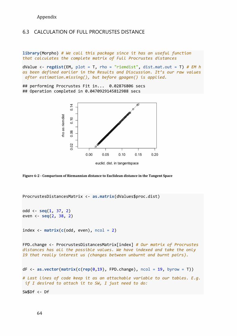
Appendix
64
6.3 CALCULATION OF FULL PROCRUSTES DISTANCE
library(Morpho) # We call this package since it has an useful function that calculates the complete matrix of Full Procrustes distances
dValue <- regdist(EM, plot = T, rho = "riemdist", dist.mat.out = T) # EM has been defined earlier in the Results and Discussion. It’s our raw values after estimation.missing(), but before gpagen() is applied.
## performing Procrustes Fit in... 0.02876806 secs ## Operation completed in 0.0470929145812988 secs
Figure 6-2 - Comparison of Riemannian distance to Euclidean distance in the Tangent Space
ProcrustesDistancesMatrix <- as.matrix(dValues$proc.dist)
odd <- seq(1, 37, 2) even <- seq(2, 38, 2)
index <- matrix(c(odd, even), ncol = 2)
FPD.change <- ProcrustesDistancesMatrix[index] # Our matrix of Procrustes distances has all the possible values. We have indexed and take the only 19 that really interest us (changes between unburnt and burnt pairs).
dF <- as.vector(matrix(c(rep(0,19), FPD.change), ncol = 19, byrow = T))
# Last lines of code keep it as an attachable variable to our tables. E.g. if I desired to attach it to SW, I just need to do:
SW$Df <- Df

UNWARPING HEATED BONES
65
6.4 QUANTITATIVE VALUES FOR WARPING AND SHRINKING
library(knitr) dt <- read.csv(file = './data/FromGM.csv', header = TRUE) kable(dt)
Table 4 - Tabulated values of Warping and Shrinking. Full Procrustes distances of unburnt-to-burnt were labeled as Warping, and the logarithm of the Centroid Size of the unburnt, minus that of the burnt was labeled as Shrinking. Provided here in case other researchers pretend to use these. In yellow we have a possible case of expansion (i.e. negative shrinking), however CEI/XXI 29 is one of the individuals with virtually mirrored pre-burnt bones, meaning this difference in size can be just due to developmental factors such as fluctuating asymmetry.
ID Age Sex Temperature Warping logCS.Before logCS.After Shrinking
5 73 F 900 0.0643099 6.658998 6.545755 0.113243
8 83 F 700 0.0477035 6.507733 6.493301 0.014432
17 85 M 900 0.0378350 6.625435 6.503362 0.122073
24 80 F 800 0.0333180 6.690679 6.679033 0.011646
26 90 F 900 0.0392534 6.573471 6.530758 0.042713
29 74 M 800 0.0264085 6.634388 6.647413 -0.013025
32 81 F 800 0.0754552 6.608055 6.434462 0.173593
35 75 M 900 0.0375362 6.602612 6.432676 0.169936
43 70 M 800 0.0202990 6.600072 6.598050 0.002022
49 85 F 850 0.0591030 6.632090 6.504667 0.127423
50 89 F 900 0.0728359 6.542426 6.389417 0.153009
51 70 M 900 0.0709073 6.680793 6.532535 0.148258
53 77 F 800 0.0433352 6.501725 6.354815 0.146910
57 85 M 900 0.0571740 6.588992 6.458196 0.130796
64 87 M 800 0.0324908 6.640177 6.613855 0.026322
65 81 F 900 0.1038588 6.544227 6.385370 0.158857
79 74 M 900 0.0494068 6.675157 6.610388 0.064769
86 78 M 1000 0.0326523 6.684702 6.586534 0.098168
97 88 F 1050 0.0432747 6.611635 6.482052 0.129583
Notice that in the case of CEI/XXI 29, 32, 49, 50, 57, 64 and 65 we couldn’t use the
pre-burnt 3D mesh, as it has been explained before, and instead mirrored versions of the
antimeres were used. Therefore the values for these individuals are possibly the most
biased in the sample and should be used with caution.

Appendix
66
6.5 R PACKAGES THAT THE CODE DEPENDS ON
Before running any code provided in this thesis, you might need to install packages
in R Studio if these were not previously in your computer, to do so, copy paste the
following code into your console and run it.
# First we make sure to load the required R packages and its dependencies: if (!require('knitr')){ install.packages('knitr', dependencies = TRUE) library(knitr) }
if (!require('rmarkdown')){ install.packages('knitr', dependencies = TRUE) library(knitr) }
options(knitr.table.format = 'markdown') if (!require('geomorph')){ install.packages('geomorph', dependencies = TRUE) library(geomorph) }
if (!require('pastecs')){ install.packages('pastecs', dependencies = TRUE) library(pastecs) }
if (!require('car')){ install.packages('car', dependencies = TRUE) library(pastecs) }
if (!require('RWeka')){ install.packages('RWeka', dependencies = TRUE) library(RWeka) }
source('./R/pts2array.R') # gets a function written in collaboration with David Navega. It reads all .pts files inside a directory into R and saves them as an array. Used to obtain data from landmark Editor.

UNWARPING HEATED BONES
67
6.6 THIN-PLATE SPLINE DEFORMATIONS
GP <- gridPar(pt.bg = 'black', pt.size = 0.5, n.col.cell = 25) # defines general graphical proprieties of the following plots.
plotRefToTarget(Shapes[,,1], Shapes[,,2], gridPars = GP, method = 'TPS') #CEIXXI05F
plotRefToTarget(Shapes[,,3], Shapes[,,4], gridPars = GP, method = 'TPS') #CEIXXI08F
plotRefToTarget(Shapes[,,5], Shapes[,,6], gridPars = GP, method = 'TPS') #CEIXXI17M
plotRefToTarget(Shapes[,,7], Shapes[,,8], gridPars = GP, method = 'TPS') #CEIXXI24F
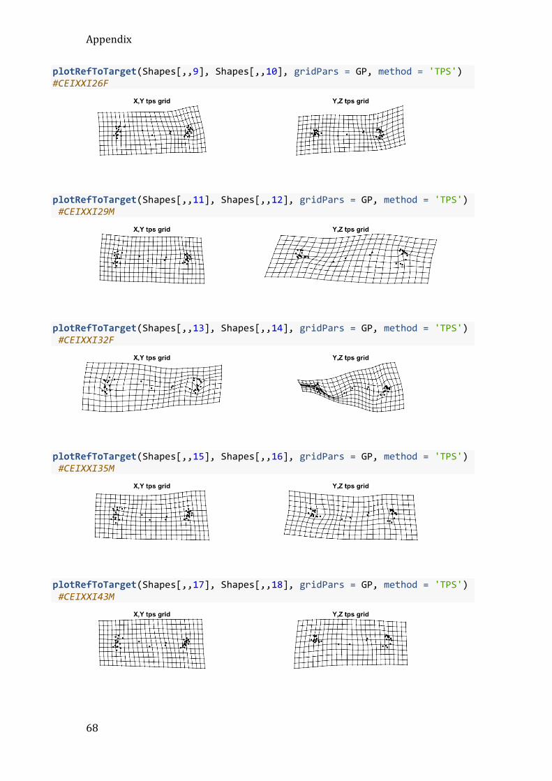
Appendix
68
plotRefToTarget(Shapes[,,9], Shapes[,,10], gridPars = GP, method = 'TPS') #CEIXXI26F
plotRefToTarget(Shapes[,,11], Shapes[,,12], gridPars = GP, method = 'TPS') #CEIXXI29M
plotRefToTarget(Shapes[,,13], Shapes[,,14], gridPars = GP, method = 'TPS') #CEIXXI32F
plotRefToTarget(Shapes[,,15], Shapes[,,16], gridPars = GP, method = 'TPS') #CEIXXI35M
plotRefToTarget(Shapes[,,17], Shapes[,,18], gridPars = GP, method = 'TPS') #CEIXXI43M

UNWARPING HEATED BONES
69
plotRefToTarget(Shapes[,,19], Shapes[,,20], gridPars = GP, method = 'TPS') #CEIXXI49F
plotRefToTarget(Shapes[,,21], Shapes[,,22], gridPars = GP, method = 'TPS') #CEIXXI50F
plotRefToTarget(Shapes[,,23], Shapes[,,24], gridPars = GP, method = 'TPS') #CEIXXI51M
plotRefToTarget(Shapes[,,25], Shapes[,,26], gridPars = GP, method = 'TPS') #CEIXXI53F
plotRefToTarget(Shapes[,,27], Shapes[,,28], gridPars = GP, method = 'TPS') #CEIXXI57M

Appendix
70
plotRefToTarget(Shapes[,,29], Shapes[,,30], gridPars = GP, method = 'TPS') #CEIXXI64M
plotRefToTarget(Shapes[,,31], Shapes[,,32], gridPars = GP, method = 'TPS') #CEIXXI65F
plotRefToTarget(Shapes[,,33], Shapes[,,34], gridPars = GP, method = 'TPS') #CEIXXI79M
plotRefToTarget(Shapes[,,35], Shapes[,,36], gridPars = GP, method = 'TPS') #CEIXXI86M
plotRefToTarget(Shapes[,,37], Shapes[,,38], gridPars = GP, method = 'TPS') #CEIXXI97F

UNWARPING HEATED BONES
71

