up in smoke: the influence of household behavior on the
TRANSCRIPT

Up in Smoke:
The Influence of Household Behavior
on the Long-Run Impact of Improved Cooking Stoves *
Rema Hanna
Esther Duflo
Michael Greenstone
WEB APPENDIX
NOT FOR PUBLICATION
A. Data Collection
In this section, we provide a comprehensive description of our data collection processes. As
shown in Appendix Figure 3, we collected baseline data from January to July 2006, prior to the
rollout of the intervention.1 The baseline survey consisted of several modules. First, we
conducted a comprehensive household module to collect data on household composition (size, as
well as each member’s age, sex, and relationship to the household head), demographics
(education levels, caste, religion), economic indicators (asset ownership, indebtedness), and
consumption patterns. As part of this module, we also collected information on the households’
stove types, stove usage, housing construction, and fuel use. After the household module was
administered, each member of the family was individually interviewed. For each child under the
age of 14, his or her primary care-giver answered a child module on his or her behalf. In this
module, we collected detailed data on stove use, such as how many meals an individual cooked
that week, as well as a series of recall questions that were designed to gauge both respiratory and
general health. For example, we collected data on whether one had a cough in the last 30 days,
whether one had a fever in the last 30 days, and health expenditures. In addition, to understand
the relationship between indoor air pollution and productivity, we collected detailed data on
employment status and time-use patterns for adults over the last 24-hours, and school enrollment
and attendance for children.
In the third, and last, component of the baseline survey, a specially trained enumeration
1 From June to November 2007, we conducted the baseline for the five villages that we added to the study.

team conducted a physical health check for each household member (both adults and children).2
The examination included detailed biometric measurements, such as height, weight, and arm
circumference. Most importantly, the examination included two tests designed to gauge
exposure to smoke and respiratory functioning. First, to gauge smoke exposure, the team
measured carbon monoxide (CO) in exhaled breath with a Micro Medical CO monitor.3 CO is a
biomarker of recent exposure to air pollution from biomass combustion, and therefore it can be
used to proxy an individual’s personal exposure to smoke from cooking stoves.
Second, we administered spirometry tests, which are designed to gauge respiratory health
by measuring how much air the lungs can hold and how well the respiratory system can move air
in and out of the lungs.4 The tests were conducted using guidelines from both the equipment
directions and American Association for Respiratory Care.5
After the initial lotteries were conducted and the stoves were built, we conducted the
Continuous Health Survey (CHS) from January 2007 to June 2008. Each household was visited
once. The survey consisted of two key modules. The first module was a household survey, in
which we collected data on whether individuals used the new stoves, whether the stoves were
used properly, whether individuals cleaned the stoves, and questions to gauge user satisfaction
with the stoves. This module also included recall questions on health for each household
member. Finally, we collected information on employment and school attendance in the last 30
2 The baseline survey was conducted by an outside survey company, while the baseline health checks were
conducted by an internally hired and trained team. Therefore, the health checks were conducted on a different
schedule as the main survey. 3 Note that we did not measure ambient pollutants (either CO or PM). Ambient measures are less interesting to
measure than exposure measures, as individuals may undertake fewer behaviors to protect themselves from smoke if
ambient measures fall and could, in fact, end up with a higher level of exposure. If we conducted only ambient
measures we would see a decline, even though their actual exposure may not have decreased due to behavioral
changes. We focused on CO, which has been argued to be a good proxy for PM. Collecting data on PM exposure is
difficult in this setting: tubes must be attached to the subjects for 24 hours and the equipment requires controlled
temperature, careful transferring of samples, and proper laboratories for testing. Given the conditions of rural
Orissa, controlling the samples would be near impossible at such a large scale. However, McCracken and Smith
(1998) report a strong correlation between the average concentrations of CO and PM2.5 in the kitchen during water
boiling tests. They conclude that this implies “the usefulness of CO measurements as an inexpensive way of
estimating PM2.5 concentrations,” even if it is not an exact proxy (see Ezzati [2002] for a discussion of this). 4 In contrast to peak flow tests, which are easier to administer, spirometry readings can be used to diagnose
obstructive lung disorders (such as chronic obstructive pulmonary disease [COPD] and asthma), and also restrictive
lung disorders. Further, they are the only way to obtain measurements of lung function that are comparable across
individuals (Beers et al., 1999). 5 A manual spirometer was used in the baseline, continuous health survey (CHS), and a portion of the midline. The
enumerators would take up to seven readings for each individual, until there were at least three satisfactory readings
and at least two FEV1 readings within 100mL or 5 percent of each other. Electronic spirometers were adopted
halfway through the midline. The new machines indicated when satisfactory readings had been completed and
saved the best reading for each individual.

days to gauge the impact of the respiratory health on productivity. The second module consisted
of the same physical health exam used in the baseline survey. However, for this survey, we only
conducted the health exam for women and children.6
From May 2008 to December 2009, we conducted the midline survey. This survey
replicated the baseline survey, collecting data on stove use, recall health, and productivity. As
part of this survey, we also conducted the health examination for all household members (men,
women, and children). Finally, the endline survey was conducted from February to December
2010. The endline survey was very similar to the baseline and midline, covering most of the
questions that were in these surveys, with some modifications based on our experiences in the
last two surveys. Specifically, we shortened the time use and household sections, and we added
more comprehensive questions on infant mortality and pregnancy outcomes. Most importantly,
we added a section on cooking and maintenance practices with the improved stoves (e.g., do
households clean the stove, do households cover both pots when cooking, do households clean
the chimney) and beliefs about the stove (e.g., whether they used more fuel, why they would
recommend it).
In addition to the main surveys, we conducted village sweeps from May 2007 to January
2010 to collect data on recent births. Specifically, we tracked pregnancies that occurred during
the scope of the study and then followed up on birth outcomes. However, we were often
prevented from gathering data soon after each birth because many women relocate to their
parents’ home in the late stages of pregnancy and road conditions were poor during periods of
monsoons. Therefore, we suspended the pregnancy sweeps before the endline survey (that
started in February 2010) and instead collected the rest of these data during the endline survey.
Besides the large-scale surveys, we conducted a number of shorter surveys to assess stove
ownership, repairs, and costs more frequently. In March and July of 2007, we conducted our
first sweeps to assess which households built a stove after Lottery 1 and whether that stove was
in good condition. We conducted these surveys and the two other similar stove surveys at the
same time as the CHS. The first Chulha Monitoring Survey (CMS) was administered from
August 2007 to January 2008 and the first Stove Survey (SS) was conducted in April 2008. Both
surveys asked households if they had built an improved stove, why they did not build one if they
6 Given that we were only able to visit each household once and that men are more difficult to find at home,
including men would have been a challenge due to attrition.

had not, and the current condition of the stove if they had. The CMS additionally obtained
information on whether stove owners used their stove properly and their perception of fuel and
time efficiency of the stove compared to the traditional stove. The second round of the CMS
overlapped with the midline survey administration and was conducted between March and
December 2009. Finally, the second round of the SS was completed between January and May
2010, during the beginning of the endline survey administration.
Note that we also meticulously collected data on stove breakages, repairs and costs for
both traditional and improved stoves in a stove cost survey that was administered concurrently
with both the midline and endline surveys.7
Lastly, throughout the project we also collected administrative data on the functioning of
this Gram Vikas program. Specifically, we collected data on lottery participation and the lottery
outcomes in each village.
B. Experimental Validity: Details
In this section, we provide a more detailed description of experimental validity tests. Appendix
Table 2A and 2B provide a test of the randomization for the baseline demographics, stove and
fuel use, and health for those identified as primary cooks and children in the baseline. In
Columns 1, 2, and 3 of both tables, we present the mean of each variable for the households that
were assigned to the pure control group (those who never won a lottery), Lottery 1 winners, and
Lottery 2 winners, respectively. Standard deviations are listed below the means in parentheses.
The difference in means between the Lottery 1 winners and the control group are presented in
Column 4, differences between Lottery 2 winners and the control group are listed in Column 5,
and differences between Lottery 1 and Lottery 2 winners are presented in Column 6, conditional
on village fixed effects. Standard errors that are clustered at the household level are shown in
parentheses in Columns 4–6. In the final row of each panel we provide the p-value for a test of
joint significance of the difference across each outcome variable.
The treatment groups appear to be generally well-balanced across the 59 baseline
characteristics that we consider. Out of the 177 differences in Columns 4–6 of both tables, only
7 We additionally administered a cost survey to shopkeepers to collect information on the market price, product life,
and repair costs for other clean stoves (i.e., LPG, mini-LPG, kerosene, and electric heaters). The addition of the
Gram Vikas cost survey in the endline provides additional data on the price of different pipes used for constructing
the improved stoves, and how much each household pays construction workers for their services.

19 (or 10 percent) are significant at the 10 percent level or more, as would be predicted by
chance. There are some notable differences in health characteristics: difference in any illness
for primary cooks between Lottery 2 and the control (Column 5) and Lottery 1 and Lottery 2
(Column 6), as well as differences in whether a child had a cough in the last 30 days between
Lottery 1 and both the control (Column 1) and Lottery 2 (Column 6). However, in testing the
joint significance of health differences for primary cooks and children, only one of the set of six
differences is significant at the 10 percent level or more (the difference between Lottery 1 and
Lottery 2 for primary cooks). Despite the fact that the data appear well-balanced, to increase
precision in the ensuing analysis on the effect of the stoves on CO exposure and health, we will
condition the regressions on the baseline values (although note that, in practice, controlling for
the baseline values does not alter the magnitude nor significance of our estimates).8
In Appendix Table 3, we test for differential attrition in each of the four main surveys
(baseline, CHS, midline, and endline). In each of the odd columns, we present the coefficient
estimates when we regress a dummy variable for survey attrition on the treatment dummy. In the
even columns, we present coefficient estimates from regressing an interaction of the treatment
dummy with a set of indicator variables for survey round. In Columns 1 and 2, we study
household attrition, while in the remaining columns we test for attrition within the sample of
individuals. All regressions are clustered at the household level and include village by survey
fixed effects. On average, we do not observe a significant difference in survey attrition for
households (Column 1) and note that the magnitude of this coefficient estimate is also near zero.
Further, we do not observe significant differences across any of the four main survey waves
(Column 2). For individuals (females, primary cooks and children), we only observe a small,
significant difference in attrition for primary cooks in the CHS and children in the baseline
(significant at the 10 percent level). In total, out of the twenty differences that we explore in this
table only two are significant at the 10 percent level, which is what one would expect by chance.
These findings suggest that differential attrition is not a source of bias in the analysis.
8 The results for women are similar to those of primary cooks. Out of the 39 differences (13 variables times three
differences) we explore for women, only four are significant (or 10 percent, which is what would be predicted by
chance). We omit them for brevity, as our subsequent health analysis will be primarily centered on primary cooks.
However, they are available upon request.

(1) (2) (3) (4) (5) (6) (7) (8) (9) (10) (11) (12) (13) (14) (15)
Carbon Monoxide FEV1
FEV1/FVC * 100 BMI
Cough or Cold Sore Eyes Headache Phlegm Wheeze Tight Chest Any Illness Health Exp.
Meals -0.008 0.004 0.100** 0.062*** -0.005 -0.009*** 0.002 -0.000 -0.001** -0.001 -0.000 1.830(0.039) (0.003) (0.042) (0.017) (0.003) (0.002) (0.003) (0.002) (0.000) (0.001) (0.002) (1.365)
N 2,001 1,685 1,646 2,127 2,464 2,464 2,464 2,463 2,463 2,463 2,464 2,214
Carbon Monoxide BMI Cough
Consult for Fever Earache
Skin Infection Vomit Weakness
Abdominal Pain
Hearing Problems
Vision Problems Worms Diarrhea Any Illness Health Exp.
Meals -0.124*** 0.006 -0.003 0.000 0.002 0.000 0.000 -0.000 0.000 0.000 0.001 0.004* -0.001 -0.002 0.010(0.047) (0.009) (0.003) (0.003) (0.002) (0.002) (0.001) (0.003) (0.002) (0.000) (0.001) (0.002) (0.001) (0.003) (0.562)
N 507 2,659 3,293 3,232 3,293 3,292 3,293 3,292 3,292 3,293 3,293 3,289 3,293 3,293 3,199Notes: This table provides the coefficients from a regression of each variable listed in the table on the number of meals cooked with a clean stove at time of baseline. All regressions are estimated using OLS, include village x month ofsurvey x year of survey fixed effects, and standard errors are clustered at the household level. For continuous variables, the top 1 percent of values are dropped. BMI for children is standardized using values from the 2000 US CDCPopulation of Children. *** p<0.01, ** p<0.05, * p<0.1
Panel A: Primary Cooks
Panel B: Children Aged 13 and Under in the Baseline
Appendix Table 1: Cross-Sectional Analysis between the Number of Meals Cooked during Last Week with a Clean Stove and Baseline Smoke Exposure and Health

Control Lottery1 Lottery2 Lottery1 - Control Lottery2 - Control Lottery1 - Lottery2 (1) (2) (3) (4) (5) (6)
Household Size 6.41 6.73 6.58 0.3548** 0.2979* 0.1802[3.18] [3.78] [3.52] (0.1591) (0.1634) (0.1787)
Monthly Per Capita Household Expenditures 470.10 475.05 483.36 9.5308 16.3650 -10.3258[295.12] [306.29] [296.15] (13.8150) (14.6623) (14.9032)
Minority Household (Scheduled Caste or Tribe) 0.40 0.42 0.48 -0.0225** 0.0006 -0.0241*[0.49] [0.49] [0.50] (0.0114) (0.0124) (0.0125)
Has Electricity in Household 0.47 0.48 0.46 0.0262 0.0180 0.0102[0.50] [0.50] [0.50] (0.0204) (0.0212) (0.0211)
Male Head Ever Attended School 0.71 0.71 0.66 0.0093 -0.0239 0.0264[0.45] [0.45] [0.47] (0.0217) (0.0248) (0.0245)
Male Head Literate 0.62 0.58 0.54 -0.0178 -0.0433 0.0183[0.49] [0.49] [0.50] (0.0249) (0.0270) (0.0273)
Female Head Ever Attended School 0.31 0.34 0.30 0.0401* -0.0030 0.0319[0.46] [0.47] [0.46] (0.0224) (0.0232) (0.0233)
Female Head Literate 0.21 0.21 0.18 0.0086 -0.0193 0.0156[0.40] [0.41] [0.39] (0.0201) (0.0204) (0.0204)
Female Has a Savings Account 0.64 0.69 0.70 0.0353 0.0311 0.0012[0.48] [0.46] [0.46] (0.0222) (0.0229) (0.0228)
P-value from Joint Test 0.09 0.79 0.31
Traditional Stove 0.989865 1.00 0.99 0.0047 -0.0014 0.0051[0.10] [0.07] [0.10] (0.0042) (0.0052) (0.0044)
Any Type of "Clean Stove" 0.228604 0.24 0.23 0.0176 0.0041 0.0028[0.42] [0.43] [0.42] (0.0192) (0.0199) (0.0199)
Improved Stove 0.012387 0.01 0.01 -0.0012 -0.0026 0.0038[0.11] [0.10] [0.07] (0.0051) (0.0049) (0.0044)
Kerosene 0.109234 0.10 0.10 -0.0034 -0.0156 0.0080[0.31] [0.31] [0.29] (0.0148) (0.0153) (0.0150)
Biogas 0.030405 0.03 0.03 -0.0045 -0.0037 -0.0049[0.17] [0.16] [0.17] (0.0070) (0.0074) (0.0072)
LPG 0.03491 0.05 0.05 0.0124 0.0116 0.0030[0.18] [0.21] [0.22] (0.0094) (0.0101) (0.0109)
Electric 0.095721 0.12 0.11 0.0270** 0.0144 0.0079[0.29] [0.32] [0.31] (0.0137) (0.0141) (0.0147)
Coal 0.004505 0.00 0.01 -0.0022 0.0002 -0.0025[0.07] [0.05] [0.07] (0.0029) (0.0036) (0.0032)
Cooked Most Meals with Traditional Stove in Last Week 0.941379 0.93 0.92 -0.0135 -0.0219* 0.0083[0.24] [0.26] [0.28] (0.0115) (0.0125) (0.0132)
Meals Cooked Last Week 13.64567 13.82 13.80 0.1659 0.2457 -0.0444[4.34] [4.02] [3.77] (0.2018) (0.2069) (0.1977)
Meals Cooked Last Week with Traditional Stove 12.63883 12.59 12.59 -0.0138 0.0867 -0.0994[4.82] [4.53] [4.57] (0.2209) (0.2332) (0.2260)
% Primary Cook Female 0.33 0.31 0.32 -0.0138 -0.0078 -0.0077[0.47] [0.46] [0.47] (0.0132) (0.0141) (0.0138)
Meals Cooked in Open Area Last Week 7.40 7.28 7.72 -0.0779 0.4041 -0.4473[7.06] [7.17] [7.31] (0.3294) (0.3475) (0.3524)
Meals Cooked in Semi-open Area Last Week 5.06 5.18 5.03 0.0744 -0.0465 0.1195[7.03] [6.84] [6.68] (0.3140) (0.3254) (0.3255)
Meals Cooked in Enclosed Area Last Week 0.83 0.94 0.79 0.0956 -0.0781 0.1429[3.19] [3.27] [3.05] (0.1551) (0.1578) (0.1605)
Ever Use Wood 0.98 0.99 0.99 0.0091 0.0023 0.0090*[0.14] [0.09] [0.12] (0.0057) (0.0066) (0.0053)
Minutes Spent Gathering Wood Yesterday (if gathered wood) 39.17 34.49 30.85 -5.4793 -8.6115 2.5935[153.17] [122.92] [124.02] (6.0091) (6.2671) (5.0401)
Wood Used for Last Meal (in kg) 4.96 5.10 4.80 0.4617 0.3894 -0.3731[6.13] [7.04] [5.57] (0.4799) (0.4716) (0.5133)
Meals Per Bundle of Wood 5.19 5.04 4.88 -0.0204 -0.0561 -0.0551[7.23] [6.06] [8.38] (0.3554) (0.4300) (0.4002)
Household Gathers Wood 0.82 0.87 0.81 0.0369** -0.0170 0.0541***[0.39] [0.34] [0.39] (0.0162) (0.0178) (0.0170)
Ever Bought Wood 0.37 0.33 0.36 -0.0195 0.0117 -0.0199[0.48] [0.47] [0.48] (0.0195) (0.0202) (0.0203)
Ever Sold Wood 0.20 0.19 0.21 -0.0117 -0.0100 -0.0015[0.40] [0.39] [0.41] (0.0139) (0.0146) (0.0142)
P-values from Joint Test 0.23 0.90 0.29
Appendix Table 2A: Randomization Check for Baseline Demographic Characteristics and Stove UseMeans Differences, Conditional on Village FE
Panel A: Demographics
Panel B: Baseline Stove Characteristics and Fuel Use

Control Lottery1 Lottery2 Lottery1 - Control Lottery2 - Control Lottery1 - Lottery2 (1) (2) (3) (4) (5) (6)
Carbon Monoxide 7.91 7.53 7.88 -0.4293 0.1240 -0.6220*[6.59] [5.68] [6.46] (0.3313) (0.3749) (0.3307)
FEV1 1.97 1.97 1.96 0.0102 -0.0006 0.0055[0.37] [0.37] [0.37] (0.0219) (0.0231) (0.0228)
FVC 2.30 2.32 2.28 0.0235 0.0028 0.0152[0.45] [0.44] [0.42] (0.0261) (0.0272) (0.0264)
FEV1/FVC 89.54 89.60 89.79 -0.0816 -0.1892 0.0325[5.92] [6.52] [5.89] (0.3541) (0.3612) (0.3786)
BMI 19.04 18.78 18.86 -0.1665 0.0078 -0.2254*[2.49] [2.55] [2.50] (0.1241) (0.1332) (0.1293)
Cold or Cough 0.53 0.49 0.54 -0.0351 0.0230 -0.0513**[0.50] [0.50] [0.50] (0.0241) (0.0251) (0.0249)
Any Illness 0.85 0.84 0.91 -0.0054 0.0541*** -0.0594***[0.36] [0.36] [0.29] (0.0174) (0.0166) (0.0164)
Phlegm 0.14 0.12 0.13 -0.0194 -0.0008 -0.0102[0.35] [0.32] [0.34] (0.0161) (0.0174) (0.0168)
Headache 0.51 0.48 0.49 -0.0316 -0.0296 0.0015[0.50] [0.50] [0.50] (0.0237) (0.0249) (0.0251)
Sore eyes 0.29 0.27 0.28 -0.0132 0.0044 -0.0095[0.46] [0.45] [0.45] (0.0215) (0.0225) (0.0224)
Wheezing 0.01 0.01 0.01 -0.0028 -0.0013 -0.0028[0.12] [0.10] [0.10] (0.0051) (0.0053) (0.0048)
Tightness in Chest 0.04 0.04 0.05 0.0028 0.0030 -0.0054[0.20] [0.21] [0.21] (0.0099) (0.0105) (0.0102)
Total Health Expenditures 70.49 73.68 66.38 4.8840 -2.9045 7.4965[187.88] [182.08] [180.75] (9.5248) (9.5478) (9.4762)
P-value from Joint Test 0.212 0.528 0.054
Carbon Monoxide 6.63 5.90 6.89 -0.4398 0.2126 -0.7463[5.48] [4.74] [5.55] (0.5464) (0.7118) (0.6406)
BMI -1.82 -1.89 -1.85 -0.0479 0.0342 -0.0772[1.30] [1.30] [1.27] (0.0704) (0.0732) (0.0707)
Cough 0.39 0.42 0.38 0.0517** -0.0026 0.0590**[0.49] [0.49] [0.49] (0.0239) (0.0255) (0.0243)
Consulted for Fever 0.28 0.25 0.28 -0.0256 -0.0204 -0.0137[0.45] [0.43] [0.45] (0.0202) (0.0221) (0.0212)
Earache 0.09 0.09 0.09 0.0102 0.0024 0.002[0.28] [0.29] [0.28] (0.0130) (0.0139) (0.0140)
Skin 0.13 0.14 0.13 0.0120 0.0009 0.0072[0.34] [0.34] [0.34] (0.0164) (0.0168) (0.0164)
Any Illness 0.73 0.73 0.74 -0.0007 -0.0102 -0.0032[0.44] [0.44] [0.44] (0.0222) (0.0227) (0.0222)
Vision Problems 0.01 0.01 0.01 -0.0038 -0.0004 -0.0011[0.12] [0.10] [0.11] (0.0046) (0.0046) (0.0046)
Hearing Problems 0.01 0.02 0.01 0.0031 -0.0034 0.0094*[0.11] [0.12] [0.10] (0.0049) (0.0047) (0.0051)
Vomiting 0.07 0.08 0.09 0.0094 0.0116 -0.0026[0.25] [0.27] [0.28] (0.0115) (0.0124) (0.0129)
Diarrhea 0.07 0.08 0.08 -0.0022 -0.0082 0.0091[0.26] [0.27] [0.27] (0.0118) (0.0129) (0.0124)
Abdominal Pain 0.14 0.15 0.14 0.0039 0.0008 0.0078[0.35] [0.35] [0.35] (0.0162) (0.0172) (0.0166)
Worms 0.09 0.11 0.09 0.0165 -0.0108 0.0209[0.28] [0.31] [0.28] (0.0144) (0.0158) (0.0157)
Weakness 0.21 0.21 0.22 -0.0100 -0.0062 -0.0066[0.41] [0.41] [0.42] (0.0192) (0.0215) (0.0203)
Total Health Expenditures 44.61 48.89 45.26 4.9607 0.7712 3.7218[101.22] [99.72] [106.05] (4.6885) (5.2102) (5.0337)
P-value from Joint Test 0.777 0.834 0.775
Appendix Table 2B: Randomization Check for Baseline CO and HealthMeans Differences, Conditional on Village FE
Panel A: Primary Cooks
Panel B: Children Under Aged 13

(1) (2) (3) (4) (5) (6)Treat 0.001 0.003 0.011
(0.006) (0.008) (0.010)Treat * Baseline 0.004 -0.001 0.031*
(0.006) (0.002) (0.017)Treat * CHS 0.011 0.030** -0.001
(0.010) (0.014) (0.012)Treat * Midline -0.007 -0.009 0.003
(0.009) (0.016) (0.017)Treat * Endline -0.004 -0.010 0.012
(0.010) (0.017) (0.016)
N 10,296 10,296 10,012 10,012 25,948 25,948Control Group Mean 0.0670 0.0670 0.136 0.136 0.354 0.354
Appendix Table 3: Testing for Survey AttritionHousehold Primary Cooks Children
Notes: This table provides results on whether there exists differential survey attrition by treatment status. Thedependent variable is a dummy variable that indicates whether the household (or individual) was not included in thesurvey. CHS is the continuous health survey conducted between the baseline and midline survey. All regressionsinclude village x survey fixed effects and standard errors are clustered at the household level. *** p<0.01, ** p<0.05, *p<0.1

Year 1 Year 2 Year 3 Year 4(1) (2) (3) (4)
Insufficient Kitchen Space/Family Size and Stove Do Not Match 0.28 0.34 0.22 0.19Does Not Want A Double Pot 0.01 0.02 0.02 0.01Already Owns a Better Stove 0.06 0.08 0.03 0.04Will Build Soon 0.27 0.21 0.38 0.15Not Interested in Building 0.07 0.15 0.06 0.26Destroyed by User 0.02 0.06 0.23 0.32Other 0.24 0.11 0.06 0.04Notes: This table provides information on why households did not have a stove, by years since stove was offered in their village.
Appendix Table 4: Reasons for Not Having a Stove, by Year of Stove Being Offered in Your Village

Gram Vikas Improved Stove
at Time of Survey
Number of Meals Cooked with any Good
Condition, Low-Polluting Stove Primary Cooks Children
(1) (2) (3) (4)
Treat * Stove in HH -0.101*** -1.333*** 0.514 -0.431(0.025) (0.421) (0.436) (0.416)
Treat * Below Median per capita Consumptio -0.015 0.202 -0.138 0.426(0.021) (0.334) (0.374) (0.344)
Treat * HH Head Any Education -0.017*** -0.116** 0.061 -0.001(0.003) (0.052) (0.053) (0.052)
Treat * HH Head Any Education (binary) -0.075*** -0.312 0.677* 0.064(0.022) (0.349) (0.378) (0.350)
Treat *Low Caste/Tribe 0.089*** 1.610*** -0.208 -0.093(0.022) (0.348) (0.399) (0.371)
Panel E: Low Caste/Tribe
Appendix Table 5: Heterogeneity in EffectsCarbon Monoxide
Panel A: Improved Stove in HH at Baseline
Panel B: Below Median per capita Consumption
Panel C: HH Head Any Education
Panel D: HH Head Any Education (binary)

Male Smokes(1)
Treat 0.009(0.009)
Treat x I(0 to 12 mo) 0.012(0.014)
Treat x I(13 to 24 mo) -0.014(0.020)
Treat x I(25 to 36 mo) 0.014(0.013)
Treat x I(37 to 48 mo) 0.014(0.015)
N 5,618
Control Group Mean 0.120
Appendix Table 6: Reduced Form Effect of Stoves on Male Smoking
Panel A: Overall Treatment Effect
Panel B: By Months Since Stove Construction

Total Number of Meals Cooked
Number of People Cooked for
Number of Minutes Spent Cooking at Arm's Length
(1) (2) (3)Treat -0.108 0.082 -0.431
(0.392) (0.112) (0.816)
N 4,663 2,677 2,625Control Group Mean 19.86 4.742 31.84
Appendix Table 7: Exploring Possible Spillovers
Notes: Using data from the midline survey, we explore the effect of being on the treatment group on thenumber of minutes spent cooking at arm's length of the stove and the number of household memberscooked for. We control for the baseline value of the variable for additional power. *** p<0.01, **p<0.05, * p<0.1
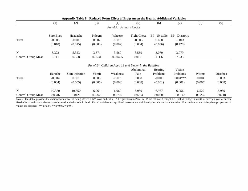
(1) (2) (3) (4) (5) (6) (7) (8) (9)
Sore Eyes Headache Phlegm Wheeze Tight Chest BP - Systolic BP - DiastolicTreat -0.005 -0.005 0.007 -0.001 -0.005 0.608 -0.013
(0.010) (0.015) (0.008) (0.002) (0.004) (0.656) (0.428)
N 5,323 5,323 3,571 3,569 3,569 3,079 3,079Control Group Mean 0.111 0.358 0.0534 0.00495 0.0171 111.6 73.35
Earache Skin Infection Vomit WeaknessAbdominal
PainHearing
ProblemsVision
Problems Worms DiarrheaTreat -0.004 0.001 0.008 -0.001 0.008 -0.000 0.004*** 0.004 0.003
(0.004) (0.005) (0.005) (0.008) (0.008) (0.001) (0.001) (0.005) (0.008)
N 10,350 10,350 6,961 6,960 6,959 6,957 6,956 6,522 6,959Control Group Mean 0.0346 0.0421 0.0343 0.0706 0.0764 0.00200 0.00143 0.0265 0.0718
Appendix Table 8: Reduced Form Effect of Program on the Health, Additional Variables
Panel A: Primary Cooks
Panel B: Children Aged 13 and Under in the Baseline
Notes: This table provides the reduced form effect of being offered a GV stove on health. All regressions in Panel A - B are estimated using OLS, include village x month of survey x year of surveyfixed effects, and standard errors are clustered at the household level. For all variables except blood pressure, we additionally include the baseline value. For continuous variables, the top 1 percent ofvalues are dropped. *** p<0.01, ** p<0.05, * p<0.1

Outcome StudyPoint
Estimate P-Value
95% Confidence
IntervalPoint
Estimate P-Value95% Confidence
IntervalPoint
Estimate P-Value95% Confidence
Interval(1) (2) (3) (4) (5) (6) (7) (8) (9) (10) (11)
Carbon Monoxide Passive Diffusion Tubes: Child (1) -52% [- 56, -47]Carbon Monoxide Passive Diffusion Tubes: Mother (1) -61% [ -65, -57]Continuous Carbon Monoxide Monitors (1) -90% [-92, -87]PM 2.5 (2) -61%
FEV (6, 12 and 18 months) (5) (5) -0.02 [ -0.09, 0.04]FVC (6, 12 and 18 months) (5) (5) -0.04 [ -0.01, 0.03](FEV1:FVC) *100 (6, 12, and 18 months) (5) (5) 0.41 [-0.44, 1.27]
SBP Estimate (2) (2) -2.3 0.30 [–6.6, 2.0] –3.7 0.10 [–8.1, 0.6]DBP Estimate (2) (2) -2.2 0.09 [–4.7, 0.3] –3.0 0.02 [–5.7, –0.4]
Mean Birth Weight (3) (3) 68 0.28 [–56, 191] 89 0.13 [–27, 204]Low Birth Weight Odds Ratio (3) (3) 0.74 [0.33, 1.66]
Field Worker Assessed Pneumonia Rate Ratio (4) 0.91 0.39 [0.74, 1.13]Field Worker Assessed Severe Pneumonia Rate Ratio (4) 0.56 0.04 [0.32, 0.97]Clinical Pneumonia Rate Ratio All (4) 0·84 0.257 [0.63, 1.13] 0.78 0.095 [0.59, 1.06]Clinical Pneumonia Rate Ratio hypoxemic (4) 0.74 0.128 [0.50, 1.09] 0.67 0.042 [0.45, 0.98]Clinical Pneumonia Rate Ratio CXR confirmed (4) 0.87 0.586 [0.52, 1.45] 0.74 0.231 [0.42, 1.15]Clinical Pneumonia Rate Ratio CXR hypoxemic (4) 0.8 0.505 [0.41, 1.56] 0.68 0.234 [0.36, 1.33]RSV(-) (4) 0.91 0.598 [0.63, 1.30] 0.79 0.192 [0.53, 1.07] RSV(-) hypoxemic (4) 0.61 0.066 [0.35 ,1.03] 0.54 0.026 [0.31, 0.91] RSV(+) (4) 0.94 0.801 [0.59, 1.49] 0.76 0.275 [0.42, 1.16] RSV(+) hypoxemic (4) 1.05 0.867 [0.60, 1.83] 0.87 0.633 [0.46, 1.51]
Cough (4) (7) (5) NSChronic Cough (4) (7) (5) NSPhlegm (4) (7) (5) NSChronic Phlegm (4) (7) (5) NSWheeze (Relative Risk) (4) (5) 0.42 [.25, .70]Tightness in Chest (4) (7) (5) NSNumber of Symptoms (Odds Ratio) (5) 0.7 0.03 [.50, .97]% Sore Eyes in Past Month (6 Month) (6) (7) (6) -19.00 S% Sore Eyes in Past Month (12 Month) (6) (7) (6) -26.10 S% Sore Eyes in Past Month (18 Month) (6) (7) (6) -26.20 S% Headache in Past Month (6 Month) (6) (7) (6) 0.00 NS% Headache in Past Month (12 Month) (6) (7) (6) -7.10 NS% Headache in Past Month (18 Month) (6) (7) (6) -20.30 S% Back pain in Past Month (6 Month) (6) (7) (6) -0.20 NS% Back pain in Past Month (12 Month) (6) (7) (6) -2.00 NS% Back pain in Past Month (18 Month) (6) (7) (6) -7.30 NS
Notes:(1) Adjusted implied controls for the number of minutes the tubes were worn.
(3) Adjusted for maternal height, gravidity, maternal diastolic blood pressure, and season of birth.(4) Information on point estimate and p-values are unavailable.(5) Paper also reports results for just 12 and 18 months of follow-up and finds similar results. These are omitted from the table for brevity.(6) The Mann-Whitney U test was used for testing the significance of differences.(7) "NS" means not significant; "S" means significant.
B. Lung Functioning
Appendix Table 9: Summary of RESPIRE FindingsEstimate Adjusted Estimate Imputed Data
A. Smoke Exposure
C. Blood Pressure
D. Infant Outcomes
E. Pneumonia and RSV Incidence for Children
F. Self Reported Symptoms
(2) Adjusted for age, BMI, daily average apparent temperature, rainy season, day of week, time of day, use of a temascal, having household electricity, an asset index, ever smoking, SHSexposure, and a random effect

Appendix Figure 1: Traditional and Gram Vikas Improved Stoves
Panel A: Traditional Stove
Panel B: Gram Vikas Improved Stove

Appendix Figure 2: Example of Gram Vikas Training Material
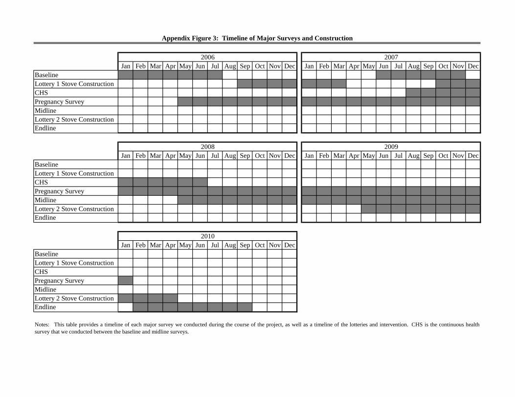
Jan Feb Mar Apr May Jun Jul Aug Sep Oct Nov Dec Jan Feb Mar Apr May Jun Jul Aug Sep Oct Nov DecBaselineLottery 1 Stove ConstructionCHSPregnancy SurveyMidlineLottery 2 Stove ConstructionEndline
Jan Feb Mar Apr May Jun Jul Aug Sep Oct Nov Dec Jan Feb Mar Apr May Jun Jul Aug Sep Oct Nov DecBaselineLottery 1 Stove ConstructionCHSPregnancy SurveyMidlineLottery 2 Stove ConstructionEndline
Jan Feb Mar Apr May Jun Jul Aug Sep Oct Nov DecBaselineLottery 1 Stove ConstructionCHSPregnancy SurveyMidlineLottery 2 Stove ConstructionEndline
Notes: This table provides a timeline of each major survey we conducted during the course of the project, as well as a timeline of the lotteries and intervention. CHS is the continuous healthsurvey that we conducted between the baseline and midline surveys.
Appendix Figure 3: Timeline of Major Surveys and Construction
2006 2007
2008 2009
2010

Panel A: Primary Household and Health Surveys
Panel B: Primary Surveys on the Condition of the Stove
Appendix Figure 4: Household Sample Sizes, By Survey
Notes: This table documents the majority of surveys that were conducted during the course of the study. HH is the number of participating households.CHS is the continuous health survey that we conducted between the baseline and midline surveys. ML is the midline survey, while EL is the endline survey.We conducted the stove costs survey in conjunction with the midline and endline. Stove status surveys provide basic information on the stoves, while stovemonitoring is a more in-depth survey of use.
Baseline Survey 2575 HH
CHS 2427 HH
ML: 2404 HH [ML Stove Cost: 2212]
EL: 2079 HH [EL Stove Cost: 2030 ]
Stove Building
Survey 2526 HH
Stove Monitoring Survey I 2281 HH
Stove Status I 2474 HH
Stove Monitoring Survey II 2377 HH
Stove Status II 2423 HH

Appendix Figure 5: Ever Had a Stove Break
41%
74%
29%
12%
67%
9%
81%
94%
0
0.1
0.2
0.3
0.4
0.5
0.6
0.7
0.8
0.9
1
Ever Destroyed
(L1)
Ever Cracked
(L1)
Ever Had Pipe Issue
(L1)
Ever Destroyed
(L2)
Ever Cracked
(L2)
Ever Had Pipe Issue
(L2)
Ever Destroyed (Control)
Ever Cracked (Control)
Traditional Stoves
Improved Stoves

Notes: This table provide sample statistics on self-reported beliefs with the GV improved cooking stoves for thosewho own one.
Appendix Figure 6: Beliefs on Stove Quality
0
0.1
0.2
0.3
0.4
0.5
0.6
0.7
0.8
Less Same More Less Same More Worse Same Better Less Same More
Time Fuel Taste Ease