updated value of service reliability estimates for ...emp.lbl.gov/sites/all/files/lbnl-6941e.pdf ·...

LBNL-6941E

Updated Value of Service Reliability Estimates for Electric Utility Customers in the United States Principal Authors Michael J. Sullivan, Josh Schellenberg, and Marshall Blundell Nexant, Inc. January 2015 The work described in this report was funded by the Office of Electricity Delivery and Energy Reliability of the U.S. Department of Energy under Contract No. DE-AC02-05CH11231.

ERNEST ORLANDO LAWRENCE BERKELEY NATIONAL LABORATORY

Disclaimer

This document was prepared as an account of work sponsored by the United States Government. While this document is believed to contain correct information, neither the United States Government nor any agency thereof, nor The Regents of the University of California, nor any of their employees, makes any warranty, express or implied, or assumes any legal responsibility for the accuracy, completeness, or usefulness of any information, apparatus, product, or process disclosed, or represents that its use would not infringe privately owned rights. Reference herein to any specific commercial product, process, or service by its trade name, trademark, manufacturer, or otherwise, does not necessarily constitute or imply its endorsement, recommendation, or favoring by the United States Government or any agency thereof, or The Regents of the University of California. The views and opinions of authors expressed herein do not necessarily state or reflect those of the United States Government or any agency thereof, or The Regents of the University of California. Ernest Orlando Lawrence Berkeley National Laboratory is an equal opportunity employer.

Updated Value of Service Reliability

Estimates for Electric Utility Customers in the United States

Michael J. Sullivan, Josh Schellenberg, and Marshall Blundell Nexant, Inc.

101 Montgomery Street, 15th Floor San Francisco, CA

January 2015

The work described in this report was funded by the Office of Electricity Delivery and Energy Reliability of the U.S. Department of Energy under Contract No. DE-AC02-05CH11231.

Acknowledgments The work described in this report was funded by the Office of Electricity Delivery and Energy Reliability, U.S. Department of Energy under Contract No. DE-AC02-05CH11231. The authors thank Joseph Paladino of the DOE Office of Electricity Delivery and Energy Reliability, and Joseph H. Eto of the Lawrence Berkeley National Laboratory for support and guidance in the development of this research. We would also like to thank Emily Fisher, Gary Fauth, Peter Larsen, Kristina Hamachi-LaCommare, Peter Cappers, and Julia Frayer for their careful reviews and comments on the earlier drafts of this report. Their comments were extremely thoughtful and useful.

Abstract

This report updates the 2009 meta-analysis that provides estimates of the value of service reliability for electricity customers in the United States (U.S.). The meta-dataset now includes 34 different datasets from surveys fielded by 10 different utility companies between 1989 and 2012. Because these studies used nearly identical interruption cost estimation or willingness-to-pay/accept methods, it was possible to integrate their results into a single meta-dataset describing the value of electric service reliability observed in all of them. Once the datasets from the various studies were combined, a two-part regression model was used to estimate customer damage functions that can be generally applied to calculate customer interruption costs per event by season, time of day, day of week, and geographical regions within the U.S. for industrial, commercial, and residential customers. This report focuses on the backwards stepwise selection process that was used to develop the final revised model for all customer classes. Across customer classes, the revised customer interruption cost model has improved significantly because it incorporates more data and does not include the many extraneous variables that were in the original specification from the 2009 meta-analysis. The backwards stepwise selection process led to a more parsimonious model that only included key variables, while still achieving comparable out-of-sample predictive performance. In turn, users of interruption cost estimation tools such as the Interruption Cost Estimate (ICE) Calculator will have less customer characteristics information to provide and the associated inputs page will be far less cumbersome. The upcoming new version of the ICE Calculator is anticipated to be released in 2015.

iv

Table of Contents

Acknowledgments.......................................................................................................................... iii

Abstract .......................................................................................................................................... iv

Table of Contents .............................................................................................................................v

List of Figures and Tables............................................................................................................. vii

Acronyms and Abbreviations ........................................................................................................ ix

Executive Summary ....................................................................................................................... xi Updated Interruption Cost Estimates ........................................................................................ xii Study Limitations ..................................................................................................................... xiv

1. Introduction ...........................................................................................................................15 1.1 Recent Interruption Cost Studies .......................................................................................16 1.2 Re-estimating Econometric Models ...................................................................................18 1.3 Overview of Model Selection Process ...............................................................................18 1.4 Variable Definitions and Units ..........................................................................................19 1.5 Report Organization ...........................................................................................................21

2. Methodology .........................................................................................................................22 2.1 Model Structure .................................................................................................................22 2.2 Summary of Model Selection Process ...............................................................................22 2.3 Details of Model Selection Process ...................................................................................24

3. Medium and Large C&I Results ...........................................................................................26 3.1 Final Model Selection ........................................................................................................26 3.2 Model Coefficients.............................................................................................................28 3.3 Comparison of 2009 and 2014 Model Estimates ...............................................................30 3.4 Interruption Cost Estimates and Key Drivers ....................................................................31

4. Small C&I Results ................................................................................................................33 4.1 Final Model Selection ........................................................................................................33 4.2 Model Coefficients.............................................................................................................35 4.3 Comparison of 2009 and 2014 Model Estimates ...............................................................37 4.4 Interruption Cost Estimates and Key Drivers ....................................................................38

5. Residential Results ................................................................................................................41 5.1 Final Model Selection ........................................................................................................41 5.2 Model Coefficients.............................................................................................................43 5.3 Comparison of 2009 and 2014 Model Estimates ...............................................................45 5.4 Interruption Cost Estimates and Key Drivers ....................................................................45

6. Study Limitations ..................................................................................................................48

v

List of Figures and Tables

Table ES-1: Estimated Interruption Cost per Event, Average kW and Unserved kWh (U.S.2013$) by Duration and Customer Class ................................................................ xii

Table ES-2: Estimated Customer Interruption Costs (U.S.2013$) by Duration, Timing of Interruption and Customer Class .................................................................................... xiii

Table 1-1: Updated Inventory of Interruption Cost Studies in the Meta-dataset .......................... 16 Figure 1-1: Overview of Model Selection Process ....................................................................... 19 Table 1-2: Units and Definitions of Variables for All Customer Classes..................................... 20 Table 1-3: Units and Definitions of Variables for C&I Customers .............................................. 20 Table 1-4: Units and Definitions of Variables for Residential Customers ................................... 21 Table 3-1: Breakdown of Categorical Variables Featured in Global Model – Medium and Large

C&I .................................................................................................................................. 26 Table 3-2: Excluded Variables and Relevant Metrics from Backwards Stepwise Selection

Process – Medium and Large C&I .................................................................................. 27 Table 3-3: Test Dataset Predictive Performance Metrics for Final and Initial Models – Medium

and Large C&I ................................................................................................................. 28 Table 3-4: Regression Output for Probit Estimation – Medium and Large C&I .......................... 28 Table 3-5: Customer Regression Output for GLM Estimation – Medium and Large C&I .......... 29 Table 3-6: Descriptive Statistics for Regression Inputs – Medium and Large C&I ..................... 29 Figure 3-1: Estimated Customer Interruption Costs (U.S.2013$) by Duration and Model .......... 30 (Summer Weekday Afternoon) – Medium and Large C&I .......................................................... 30 Table 3-7: Estimated Customer Interruption Costs (U.S.2013$) by Duration and Timing of

Interruption – Medium and Large C&I ........................................................................... 31 Table 3-8: Cost per Event, Average kW and Unserved kWh – Medium and Large C&I ............ 31 Figure 3-2: Estimated Summer Customer Interruption Costs (U.S.2013$) by Duration and

Industry – Medium and Large C&I ................................................................................. 32 Figure 3-3: Estimated Summer Customer Interruption Costs (U.S.2013$) by Duration and

Average Demand (kW/hr) – Medium and Large C&I .................................................... 32 Table 4-1: Excluded Variables and Relevant Metrics from Backwards Stepwise Selection

Process – Small C&I ....................................................................................................... 34 Table 4-2: Breakdown of Categorical Variables Featured in Final Model – Small C&I ............. 34 Table 4-3: Test Dataset Predictive Performance Metrics for Final and Initial Models – Small C&I

......................................................................................................................................... 35 Table 4-4: Customer Regression Output for Probit Estimation – Small C&I .............................. 35 Table 4-5: Customer Regression Output for GLM Estimation – Small C&I ............................... 36 Table 4-6: Descriptive Statistics for Regression Inputs – Small C&I .......................................... 37 Figure 4-1: Estimated Customer Interruption Costs (U.S.2013$) by Duration and Model .......... 38 (Summer Weekday Afternoon) – Small C&I ............................................................................... 38 Table 4-7: Estimated Customer Interruption Costs (U.S.2013$) by Duration and Timing of

Interruption – Small C&I ................................................................................................ 39 Table 4-8: Cost per Event, Average kW and Unserved kWh – Small C&I .................................. 39 Figure 4-2: Estimated Summer Afternoon Customer Interruption Costs (U.S.2013$) by Duration

and Industry – Small C&I ............................................................................................... 40 Figure 4-3: Estimated Summer Afternoon Customer Interruption Costs (U.S.2013$) by Duration

and Average Demand (kW/hr) – Small C&I ................................................................... 40

vii

Table 5-1: Breakdown of Categorical Variables Featured in Global Model – Residential .......... 41 Table 5-2: Excluded Variables and Relevant Metrics from Backwards Stepwise Selection

Process – Residential ....................................................................................................... 42 Table 5-3: Test Dataset Predictive Performance Metrics for Final and Initial Models –

Residential ....................................................................................................................... 43 Table 5-4: Regression Output for Probit Estimation – Residential .............................................. 43 Table 5-5: Regression Output for GLM Estimation – Residential ............................................... 44 Table 5-6: Descriptive Statistics for Regression Inputs – Residential .......................................... 44 Figure 5-1: Estimated Customer Interruption Costs (U.S.2013$) by Duration and Model .......... 45 (Summer Weekday Afternoon) – Residential ............................................................................... 45 Table 5-7: Estimated Customer Interruption Costs (U.S.2013$) by Duration and Timing of

Interruption – Residential ................................................................................................ 46 Table 5-8: Cost per Event, Average kW and Unserved kWh – Residential ................................. 46 Figure 5-2: Estimated Summer Afternoon Customer Interruption Costs (U.S.2013$) by Duration

and Household Income – Residential .............................................................................. 47 Figure 5-3: Estimated Summer Afternoon Customer Interruption Costs (U.S.2013$) by Duration

and Average Demand (kW/hr) – Residential .................................................................. 47

viii

Acronyms and Abbreviations

AIC Akaike’s Information Criterion

C&I Commercial and Industrial

GLM Generalized Linear Model

ICE Interruption Cost Estimate

MAE Mean Absolute Error

OLS Ordinary Least Squares

RMSE Root Mean Square Error

ix

Executive Summary

In 2009, Freeman, Sullivan & Co. (now Nexant) conducted a meta-analysis that provided estimates of the value of service reliability for electricity customers in the United States (U.S.). These estimates were obtained by analyzing the results from 28 customer value of service reliability studies conducted by 10 major U.S. electric utilities over the 16-year period from 1989 to 2005. Because these studies used nearly identical interruption cost estimation or willingness-to-pay/accept methods, it was possible to integrate their results into a single meta-dataset describing the value of electric service reliability observed in all of them. The meta-analysis and its associated econometric models were summarized in a report entitled “Estimated Value of Service Reliability for Electric Utility Customers in the United States,”1 which was prepared for Lawrence Berkeley National Laboratory (LBNL) and the Office of Electricity Delivery and Energy Reliability of the U.S. Department of Energy (DOE). The econometric models were subsequently integrated into the Interruption Cost Estimate (ICE) Calculator (available at icecalculator.com), which is an online tool designed for electric reliability planners at utilities, government organizations or other entities that are interested in estimating interruption costs and/or the benefits associated with reliability improvements (also funded by LBNL and DOE). Since the report was finalized in June 2009 and the ICE Calculator was released in July 2011, Nexant, LBNL, DOE, and ICE Calculator users have identified several ways to improve the interruption cost estimates and the ICE Calculator user experience. These improvements include:

• Incorporating more recent utility interruption cost studies;

• Enabling the ICE Calculator to provide estimates for power interruptions lasting longer than eight hours;

• Reducing the amount of detailed customer characteristics information that ICE Calculator users must provide;

• Subjecting the econometric model selection process to rigorous cross-validation techniques, using the most recent model validation methods;2 and

• Providing a batch processing feature that allows the user to save results and modify inputs.

These improvements will be addressed through this updated report and the upcoming new version of the ICE Calculator, which is anticipated to be released in 2015. This report provides updated value of service reliability estimates and details the revised econometric model, which is based on a meta-analysis that includes two new interruption cost studies. The upcoming new version of the ICE Calculator will incorporate the revised econometric model and include a batch processing feature that will allow the user to save results and modify inputs.

1 Sullivan, M.J., M. Mercurio, and J. Schellenberg (2009). Estimated Value of Service Reliability for Electric Utility Customers in the United States. Lawrence Berkeley National Laboratory Report No. LBNL-2132E. 2 For a discussion of these methods, see: Varian, Hal R. “Big Data: New Tricks for Econometrics.” Journal of Economic Perspectives. Volume 28, Number 2. Spring 2014. Pages 3–28. Available here: http://pubs.aeaweb.org/doi/pdfplus/10.1257/jep.28.2.3

xi

http://pubs.aeaweb.org/doi/pdfplus/10.1257/jep.28.2.3

Updated Interruption Cost Estimates

For each customer class, Table ES-1 provides the three key metrics that are most useful for planning purposes. These metrics are:

• Cost per event (cost for an individual interruption for a typical customer3); • Cost per average kW (cost per event normalized by average demand); and • Cost per unserved kWh (cost per event normalized by the expected amount of unserved

kWh for each interruption duration). Cost per unserved kWh is relatively high for a momentary interruption because the expected amount of unserved kWh over a 5-minute period is relatively low. In general, even though the econometric model has been considerably simplified, it produces similar estimates to those of the 2009 model. As in the 2009 study, medium and large C&I customers have the highest interruption costs, but when normalized by average kW, interruption costs are highest in the small C&I customer class. On both an absolute and normalized basis, residential customers experience the lowest costs as a result of a power interruption.

Table ES-1: Estimated Interruption Cost per Event, Average kW and Unserved kWh (U.S.2013$) by Duration and Customer Class

Interruption Cost Interruption Duration

Momentary 30 Minutes 1 Hour 4 Hours 8 Hours 16 Hours Medium and Large C&I (Over 50,000 Annual kWh)

Cost per Event $12,952 $15,241 $17,804 $39,458 $84,083 $165,482

Cost per Average kW $15.9 $18.7 $21.8 $48.4 $103.2 $203.0

Cost per Unserved kWh $190.7 $37.4 $21.8 $12.1 $12.9 $12.7

Small C&I (Under 50,000 Annual kWh)

Cost per Event $412 $520 $647 $1,880 $4,690 $9,055

Cost per Average kW $187.9 $237.0 $295.0 $857.1 $2,138.1 $4,128.3

Cost per Unserved kWh $2,254.6 $474.1 $295.0 $214.3 $267.3 $258.0

Residential

Cost per Event $3.9 $4.5 $5.1 $9.5 $17.2 $32.4



Table ES-2 shows how customer interruption costs vary by season and time of day, based on the key drivers of interruption costs that were identified in the model selection process. For medium and large C&I customers, interruption costs only meaningfully vary by season (summer vs. non-summer). For medium and large C&I customers, the cost of a summer power interruption is

3 The interruption costs in Table ES- 1 are for the average-sized customer in the meta-database. The average annual kWh usages for the respondents in the meta-database are 7,140,501 kWh for medium and large C&I customers, 19,214 kWh for small C&I customers and 13,351 kWh for residential customers.

xii

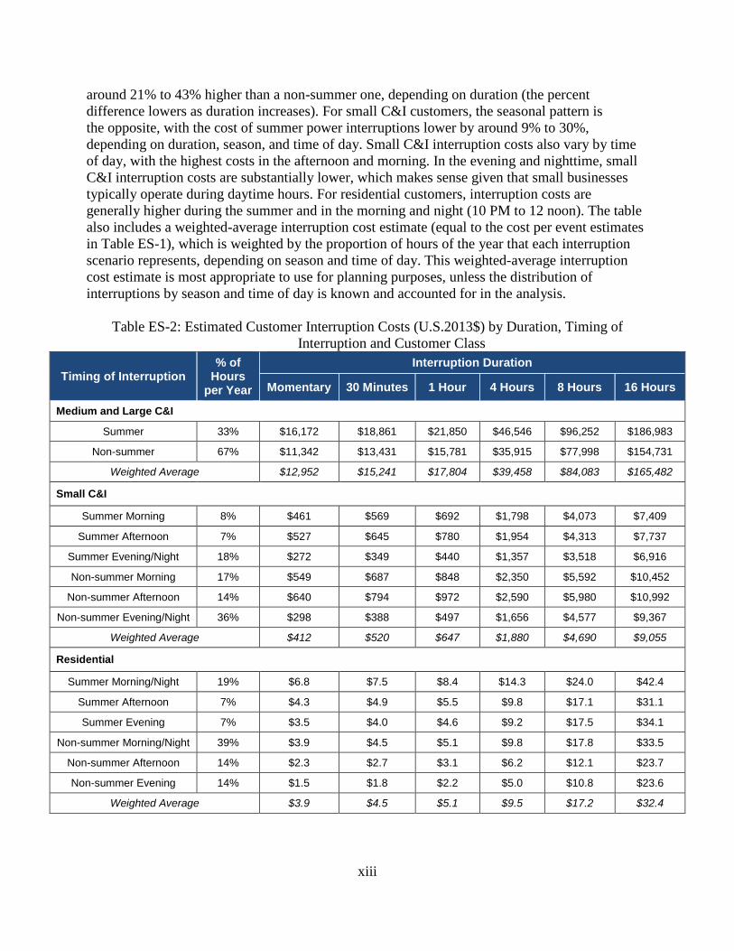
around 21% to 43% higher than a non-summer one, depending on duration (the percent difference lowers as duration increases). For small C&I customers, the seasonal pattern is the opposite, with the cost of summer power interruptions lower by around 9% to 30%, depending on duration, season, and time of day. Small C&I interruption costs also vary by time of day, with the highest costs in the afternoon and morning. In the evening and nighttime, small C&I interruption costs are substantially lower, which makes sense given that small businesses typically operate during daytime hours. For residential customers, interruption costs are generally higher during the summer and in the morning and night (10 PM to 12 noon). The table also includes a weighted-average interruption cost estimate (equal to the cost per event estimates in Table ES-1), which is weighted by the proportion of hours of the year that each interruption scenario represents, depending on season and time of day. This weighted-average interruption cost estimate is most appropriate to use for planning purposes, unless the distribution of interruptions by season and time of day is known and accounted for in the analysis.

Table ES-2: Estimated Customer Interruption Costs (U.S.2013$) by Duration, Timing of Interruption and Customer Class

Timing of Interruption % of

Hours per Year

Interruption Duration

Momentary 30 Minutes 1 Hour 4 Hours 8 Hours 16 Hours

Medium and Large C&I

Summer 33% $16,172 $18,861 $21,850 $46,546 $96,252 $186,983

Non-summer 67% $11,342 $13,431 $15,781 $35,915 $77,998 $154,731

Weighted Average $12,952 $15,241 $17,804 $39,458 $84,083 $165,482

Small C&I

Summer Morning 8% $461 $569 $692 $1,798 $4,073 $7,409

Summer Afternoon 7% $527 $645 $780 $1,954 $4,313 $7,737

Summer Evening/Night 18% $272 $349 $440 $1,357 $3,518 $6,916

Non-summer Morning 17% $549 $687 $848 $2,350 $5,592 $10,452

Non-summer Afternoon 14% $640 $794 $972 $2,590 $5,980 $10,992

Non-summer Evening/Night 36% $298 $388 $497 $1,656 $4,577 $9,367

Weighted Average $412 $520 $647 $1,880 $4,690 $9,055

Residential

Summer Morning/Night 19% $6.8 $7.5 $8.4 $14.3 $24.0 $42.4

Summer Afternoon 7% $4.3 $4.9 $5.5 $9.8 $17.1 $31.1

Summer Evening 7% $3.5 $4.0 $4.6 $9.2 $17.5 $34.1

Non-summer Morning/Night 39% $3.9 $4.5 $5.1 $9.8 $17.8 $33.5

Non-summer Afternoon 14% $2.3 $2.7 $3.1 $6.2 $12.1 $23.7

Non-summer Evening 14% $1.5 $1.8 $2.2 $5.0 $10.8 $23.6

Weighted Average $3.9 $4.5 $5.1 $9.5 $17.2 $32.4

xiii

Study Limitations

As in the 2009 study, there are limitations to how the data from this meta-analysis should be used. It is important to fully understand these limitations, so they are further described in this section and in more detail in Section 6. These limitations are:

• Certain very important variables in the data are confounded among the studies we examined. In particular, region of the country and year of the study are correlated in such a way that it is impossible to separate the effects of these two variables on customer interruption costs;

• There is further correlation between regions and scenario characteristics. The sponsors of the interruption cost studies were generally interested in measuring interruption costs for conditions that were important for planning their specific systems. As a result, interruption conditions described in the surveys for a given region tended to focus on periods of time when interruptions were more problematic for that region;

• A further limitation of our research is that the surveys that formed the basis of the studies we examined were limited to certain parts of the country. No data were available from the northeast/mid-Atlantic region, and limited data were available for cities along the Great Lakes;

• Another caveat is that around half of the data from the meta-database is from surveys that are 15 or more years old. Although the intertemporal analysis in the 2009 study showed that interruption costs have not changed significantly over time, the outdated vintage of the data presents concerns that, in addition to the limitations above, underscore the need for a coordinated, nationwide effort that collects interruption cost estimates for many regions and utilities simultaneously, using a consistent survey design and data collection method; and

• Finally, although the revised model is able to estimate costs for interruptions lasting longer than eight hours, it is important to note that the estimates in this report are not appropriate for resiliency planning. This meta-study focuses on the direct costs that customers experience as a result of relatively short power interruptions of up to 24 hours at most. For resiliency considerations that involve planning for long duration power interruptions of 24 hours or more, the nature of costs change and the indirect, spillover effects to the greater economy must be considered.4 These factors are not captured in this meta-analysis.

4 For a detailed study and literature review on estimating the costs associated with long duration power interruptions lasting 24 hours to 7 weeks, see: Sullivan, Michael and Schellenberg, Josh. Downtown San Francisco Long Duration Outage Cost Study. March 27, 2013. Prepared for Pacific Gas & Electric Company.

xiv

1. Introduction

In 2009, Freeman, Sullivan & Co. (now Nexant) conducted a meta-analysis that provided estimates of the value of service reliability for electricity customers in the United States (U.S.). These estimates were obtained by analyzing the results from 28 customer value of service reliability studies conducted by 10 major U.S. electric utilities over the 16-year period from 1989 to 2005. Because these studies used nearly identical interruption cost estimation or willingness-to-pay/accept methods, it was possible to integrate their results into a single meta-dataset describing the value of electric service reliability observed in all of them. Once the datasets from the various studies were combined, a two-part regression model was used to estimate customer damage functions that can be generally applied to calculate customer interruption costs per event by season, time of day, day of week, and geographical regions within the U.S. for industrial, commercial, and residential customers. The meta-analysis and its associated econometric models were summarized in a report entitled “Estimated Value of Service Reliability for Electric Utility Customers in the United States,”5 which was prepared for Lawrence Berkeley National Laboratory (LBNL) and the Office of Electricity Delivery and Energy Reliability of the U.S. Department of Energy (DOE). The econometric models were subsequently integrated into the Interruption Cost Estimate (ICE) Calculator (available at icecalculator.com), which is an online tool designed for electric reliability planners at utilities, government organizations or other entities that are interested in estimating interruption costs and/or the benefits associated with reliability improvements (also funded by LBNL and DOE). Since the report was finalized in June 2009 and the ICE Calculator was released in July 2011, Nexant, LBNL, DOE, and ICE Calculator users have identified several ways to improve the interruption cost estimates and the ICE Calculator user experience. These improvements include:

• Incorporating more recent utility interruption cost studies;

• Enabling the ICE Calculator to provide estimates for power interruptions lasting longer than eight hours;

• Reducing the amount of detailed customer characteristics information that ICE Calculator users must provide;

• Subjecting the econometric model selection process to rigorous cross-validation techniques, using the most recent model validation methods;6 and

• Providing a batch processing feature that allows the user to save results and modify inputs.

These improvements will be addressed through this updated report and the upcoming new version of the ICE Calculator, which is anticipated to be released in 2015. This report provides updated value of service reliability estimates and details the revised econometric model, which is based on a meta-analysis that includes two new interruption cost studies. The upcoming new

5 Sullivan, M.J., M. Mercurio, and J. Schellenberg (2009). Estimated Value of Service Reliability for Electric Utility Customers in the United States. Lawrence Berkeley National Laboratory Report No. LBNL-2132E. 6 For a discussion of these methods, see: Varian, Hal R. “Big Data: New Tricks for Econometrics.” Journal of Economic Perspectives. Volume 28, Number 2. Spring 2014. Pages 3–28. Available here: http://pubs.aeaweb.org/doi/pdfplus/10.1257/jep.28.2.3

15


version of the ICE Calculator will incorporate the revised econometric model and include a batch processing feature that will allow the user to save results and modify inputs. 1.1 Recent Interruption Cost Studies

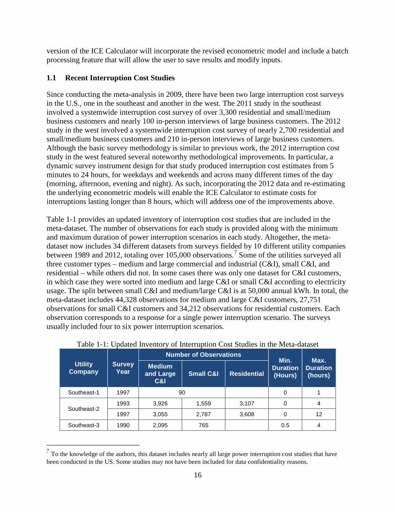
Since conducting the meta-analysis in 2009, there have been two large interruption cost surveys in the U.S., one in the southeast and another in the west. The 2011 study in the southeast involved a systemwide interruption cost survey of over 3,300 residential and small/medium business customers and nearly 100 in-person interviews of large business customers. The 2012 study in the west involved a systemwide interruption cost survey of nearly 2,700 residential and small/medium business customers and 210 in-person interviews of large business customers. Although the basic survey methodology is similar to previous work, the 2012 interruption cost study in the west featured several noteworthy methodological improvements. In particular, a dynamic survey instrument design for that study produced interruption cost estimates from 5 minutes to 24 hours, for weekdays and weekends and across many different times of the day (morning, afternoon, evening and night). As such, incorporating the 2012 data and re-estimating the underlying econometric models will enable the ICE Calculator to estimate costs for interruptions lasting longer than 8 hours, which will address one of the improvements above. Table 1-1 provides an updated inventory of interruption cost studies that are included in the meta-dataset. The number of observations for each study is provided along with the minimum and maximum duration of power interruption scenarios in each study. Altogether, the meta-dataset now includes 34 different datasets from surveys fielded by 10 different utility companies between 1989 and 2012, totaling over 105,000 observations.7 Some of the utilities surveyed all three customer types – medium and large commercial and industrial (C&I), small C&I, and residential – while others did not. In some cases there was only one dataset for C&I customers, in which case they were sorted into medium and large C&I or small C&I according to electricity usage. The split between small C&I and medium/large C&I is at 50,000 annual kWh. In total, the meta-dataset includes 44,328 observations for medium and large C&I customers, 27,751 observations for small C&I customers and 34,212 observations for residential customers. Each observation corresponds to a response for a single power interruption scenario. The surveys usually included four to six power interruption scenarios.

Table 1-1: Updated Inventory of Interruption Cost Studies in the Meta-dataset

Utility Company

Survey Year

Number of Observations Min.

Duration (Hours)

Max. Duration (hours)

Medium and Large

C&I Small C&I Residential

Southeast-1 1997 90 0 1

Southeast-2 1993 3,926 1,559 3,107 0 4

1997 3,055 2,787 3,608 0 12

Southeast-3 1990 2,095 765 0.5 4

7 To the knowledge of the authors, this dataset includes nearly all large power interruption cost studies that have been conducted in the US. Some studies may not have been included for data confidentiality reasons.

16

Utility Company

Survey Year

Number of Observations Min.

Duration (Hours)

Max. Duration (hours)

Medium and Large

C&I Small C&I Residential

2011 7,941 2,480 3,969 1 8

Midwest-1 2002 3,171 0 8

Midwest-2 1996 1,956 206 0 4

West-1 2000 2,379 3,236 3,137 1 8

West-2

1989 2,025 5 0 4

1993 1,790 825 2,005 0 4

2005 3,052 3,223 4,257 0 8

2012 5,342 4,632 4,106 0 24

Southwest 2000 3,991 2,247 3,598 0 4

Northwest-1 1989 2,210 2,126 0.25 8

Northwest-2 1999 7,091 4,299 0 12

= Recently incorporated data

Prior to adding the 2012 West-2 survey, the meta-dataset included power interruption scenarios with durations of up to 12 hours. However, the 2009 model for each customer class estimated interruption costs that reached a maximum at 8 hours, and then the estimated interruption costs would decrease, which indicated that the prior model clearly did not provide reliable predictions beyond 8 hours (i.e., it is unreasonable that a 9-hour power interruption would cost less than an 8-hour one). As discussed in Sections 3 through 5, for interruptions from 8 to 16 hours, the new model produces estimates that are more reasonable and show gradually increasing costs up to 16 hours. This improvement in model performance is attributed to the addition of the 24-hour interruption scenarios (2012 West-2) and to the much simpler model specification that resulted from the rigorous selection process. Although the revised model is able to estimate costs for interruptions lasting longer than 8 hours, it is important to note that the estimates in this report are not appropriate for resiliency planning. This meta-study focuses on the direct costs that customers experience as a result of relatively short power interruptions of up to 24 hours at most. In fact, the final models and results that are presented in Sections 3 through 5 truncate the estimates at 16 hours, due to the relatively few number of observations beyond 12 hours (scenarios of more than 12 hours account for around 2% to 3% of observations for all customer classes). For resiliency considerations that involve planning for long duration power interruptions of 24 hours or more, the nature of costs change and the indirect, spillover effects to the greater economy must be considered.8 These factors are not captured in this meta-analysis.


17

As discussed in Section 6, another caveat is that this meta-analysis may not accurately reflect current interruption costs, given that around half of the data in the meta-database is from surveys that are 15 or more years old. To address this issue, the 2009 study included an intertemporal analysis, which suggested that interruption costs did not change significantly throughout the 1990s and early 2000s. However, during the past decade in particular, technology trends may have led to an increase in interruption costs. For example, home and business life has become increasingly reliant on data centers and “cloud” computing, which may have led to an increase in interruption costs for both producers and consumers of these services. Therefore, the outdated vintage of the data presents concerns that underscore the need for a coordinated, nationwide effort that collects interruption cost estimates for many regions and utilities simultaneously, using a consistent survey design and data collection method. 1.2 Re-estimating Econometric Models

Using the new meta-dataset, Nexant re-estimated the econometric models that relate interruption costs to duration, customer characteristics such as annual kWh, and other factors. Nexant then compared the results of the original model specification to those of several alternatives that included a reduced number of variables. This model selection process addressed another ICE Calculator improvement – reducing the amount of detailed customer characteristics information that ICE Calculator users must provide, which has been a significant barrier to the tool’s use. When the econometric models were originally estimated in 2009, statistical significance was the focus of the analysis and, due to the large number of observations in the meta-dataset, many of the customer characteristics variables were statistically significant in the model, even if the marginal effect of the variable was negligible and/or collinear with other variables. Basically, many of the variables in the original specification were statistically significant, but not practically significant. In re-estimating the models, Nexant focused on the practical significance of each variable by conducting sensitivity tests to determine which variables have a substantive impact on the interruption cost estimates. Nexant also employed more recent model selection methods that have been developed since 2009, which significantly improved the rigor with which variables were selected for the model. This process led to a more parsimonious model that only included key variables. In turn, ICE Calculator users will have less customer characteristics information to provide and the associated inputs page will be far less cumbersome. 1.3 Overview of Model Selection Process

Figure 1-1 provides an overview of the model selection process. The entire dataset of interruption cost estimates for each customer class is first randomly divided into a test dataset (10% of the entire dataset) and a training dataset (the remaining 90%). The training dataset is used to train the model, which refers to the process of selecting variables for the final specification. The test dataset is excluded from the model training process so that it can be used as a test of the final model performance on unseen data, which refers to data that is completely separate from the model training process. Next, the training dataset is randomly divided into 10 equally sized parts. Then, each candidate model specification is estimated on nine of 10 parts of the training dataset. The estimated coefficients for each candidate model specification are subsequently used to predict interruption costs on the tenth part of the training dataset. This process, which is referred to as 10-fold cross-validation, is repeated nine times while withholding one of the remaining nine parts of the training dataset each time. Relevant accuracy metrics for

18

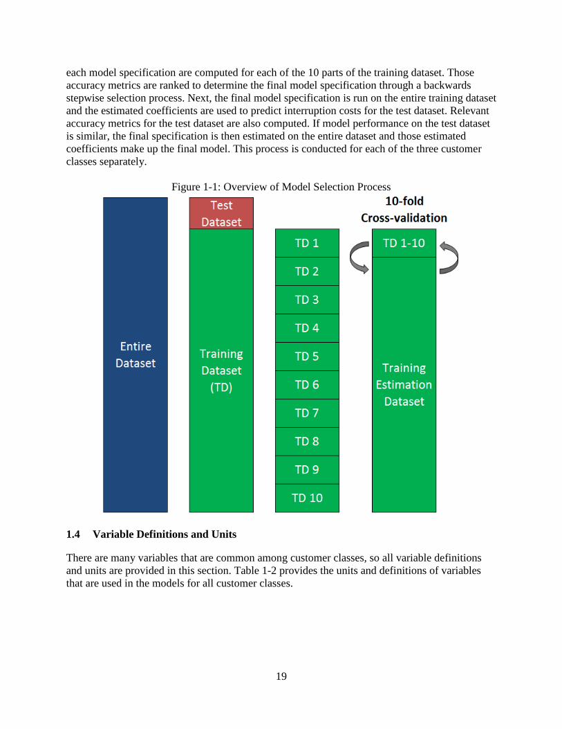
each model specification are computed for each of the 10 parts of the training dataset. Those accuracy metrics are ranked to determine the final model specification through a backwards stepwise selection process. Next, the final model specification is run on the entire training dataset and the estimated coefficients are used to predict interruption costs for the test dataset. Relevant accuracy metrics for the test dataset are also computed. If model performance on the test dataset is similar, the final specification is then estimated on the entire dataset and those estimated coefficients make up the final model. This process is conducted for each of the three customer classes separately.

Figure 1-1: Overview of Model Selection Process

1.4 Variable Definitions and Units

There are many variables that are common among customer classes, so all variable definitions and units are provided in this section. Table 1-2 provides the units and definitions of variables that are used in the models for all customer classes.

19

Table 1-2: Units and Definitions of Variables for All Customer Classes Variable

Name Variable Definition Units

annual MWh Annual MWh of customer MWh

duration Duration of power interruption scenario Minutes

time of day Time of day of power interruption scenario Categorical – Morning (6 AM to 12 PM);

Afternoon (12 to 5 PM; Evening (5 to 10 PM); Night (10 PM to 6 AM)

weekday Time of week of power interruption scenario Binary – Weekday = 1; Weekend = 0

summer Time of year of power interruption scenario Binary – Summer = 1; Non-summer = 0

warning Whether power interruption scenario had advance warning Binary – Warning = 1; No warning = 0

Table 1-3 provides the units and definitions of variables that are used in the models for both the small and medium/large C&I customer classes. For both C&I customer classes, the model selection process begins with separate variables for all eight of the industry groups in the table, with Agriculture, Forestry & Fishing as the reference category by default. However, given that each industry group is tested separately for inclusion in the model, only one or two industry variables may remain in the final model, in which case the dropped industry variables are relegated to the reference category. Within the reference category, there may be multiple industries with presumably varying interruption costs, but if the model selection process has shown that there are not any meaningful differences within the industries in the reference category, those industry variables will be grouped together. The same logic applies for other categorical variables.

Table 1-3: Units and Definitions of Variables for C&I Customers Variable


industry Customer business type, based on NAICS or SIC code

Categorical – Agriculture, Forestry & Fishing; Mining; Construction; Manufacturing;

Transportation, Communication & Utilities; Wholesale & Retail Trade; Finance, Insurance

& Real Estate; Services; Public Administration; Unknown

backup equipment Presence of backup equipment at facility

Categorical – None; Backup Gen or Power Conditioning; Backup Gen and Power

Conditioning

Finally, Table 1-4 provides the units and definitions of variables that are only used in the residential customer models.

20

Table 1-4: Units and Definitions of Variables for Residential Customers Variable


household income Household income $

medical equip. Presence of medical equipment in home Binary – Medical equipment = 1; No medical equipment = 0

backup generation Presence of backup generation in home Binary – Backup = 1; No backup = 0

outage in last 12 months Interruption of longer than 5 minutes within past year Binary – Yes = 1; No = 0

# residents X-Y Number of residents in home within X-Y age range Number of people

housing Type of housing Categorical – Detached; Attached;

Apartment/Condo; Mobile; Manufactured; Unknown

1.5 Report Organization

The remainder of this report proceeds as follows. Section 2 summarizes the regression modeling methodology and selection process that applies to all three customer classes – medium and large C&I, small C&I and residential. This is followed by three sections that describe the final model selection and provide the final regression coefficients for each customer class. Finally, Section 6 describes some of the study’s limitations.

21

2. Methodology

This section summarizes the study methodology, including the regression model structure and selection process. 2.1 Model Structure

A two-part regression model was used to estimate the customer interruption cost functions (also referred to as customer damage functions). This is the same class of model used in the previous meta-study. The two-part model assumes that the zero values in the distribution of interruption costs are correctly observed zero values, rather than censored values. In the first step, a probit model is used to predict the probability that a particular customer will report any positive value versus a value of zero for a particular interruption scenario. This model is based on a set of independent variables that describe the nature of the interruption as well as customer characteristics. The predicted probabilities from this first stage are retained. In the second step, using a generalized linear model (GLM), interruption costs for only those customers who report positive costs are related to the same set of independent variables used in the first stage. Predictions are made from this model for all observations, including those with a reported interruption cost of zero. Finally, the predicted probabilities from the first part are multiplied by the estimated interruption costs from the second part to generate the final interruption cost predictions. The functional form for the second part of the two-part model must take into account that the interruption cost distribution is bounded at zero and extremely right skewed (i.e. it has a long tail in the upper end of the distribution). Ordinary least squares (OLS) is not an appropriate functional form given these conditions. A simple way to define the customer damage function given the above constraints is to estimate the mean interruption cost, which is linked to the predictor variables through a logarithmic link function using a GLM. The parameter values in the two-part model cannot be directly interpreted in terms of their influence on interruption costs because the relationships are among the variables in their logarithms. However, the estimated model produces a predicted interruption cost, given the values of variables in the models. To analyze the magnitude of the impact of variables in the model on interruption cost, it is necessary to compare the predictions made by the function under varying assumptions. For example, it is possible to observe the effect of duration on interruption cost by holding the other variables constant at their sample means. In this way one can predict average customer interruption costs of varying durations holding other factors constant statistically. For a more detailed discussion of the two-part model, its functional form and the reasons why it is most appropriate for this type of data, refer to the methodology section of the 2009 report. 2.2 Summary of Model Selection Process

Nexant aimed to estimate a more parsimonious model that only included key predictor variables. This facilitates interruption cost estimation by simplifying the ICE Calculator interface and

22

reducing the burden that ICE Calculator users face in providing numerous, accurate customer characteristics information. This section first outlines the steps involved in the model selection process that Nexant undertook, followed by a more detailed exposition of the problem at hand, and a justification for the method. To select a more parsimonious model, Nexant conducted the following steps for each of the three customer classes:

1. Randomly sample 10% of the data and hold it out as the test dataset (assign other 90% as the training dataset);

2. Split training dataset into 10 randomly assigned, equally sized parts;

3. Start with the original specification (the global model) and identify model variables that are candidates for removal (all variables except ineligible lower power terms);

4. Remove one of the eligible model variables to yield a new model;

5. Estimate model on nine of 10 parts of the training dataset and retain estimates;

6. Use retained estimates from step 5 to predict on the tenth part of the training dataset, computing relevant accuracy metrics;

7. Repeat steps 5 and 6, cycling over each of the remaining 9 parts of the training dataset;

8. Take the average and standard deviation of the accuracy metrics from the predictions for each of 10 parts of the training dataset;

9. Repeat steps 4 through 8, for each possible candidate variable for removal;

10. Use saved accuracy metrics to rank models;

11. Exclude from the global model the variable, which when dropped, produced estimates that outperformed the rest;

12. Repeat steps 2 through 11 until only a constant remains;

13. Inspect results and select model that is parsimonious, yet sufficiently accurate according to the out-of-sample accuracy metrics described above; and

14. Test final model against the original global model using the test dataset to estimate model’s performance on unseen data (ensures that the model predicts well for data that was not included in the model training process).

As discussed in Section 1, this model selection process draws from the recent model selection methods that have been developed since 2009,9 which significantly improves the rigor with which variables are selected for the model. The remainder of this section describes this process in more detail.

9 For a discussion of these methods, see: Varian, Hal R. “Big Data: New Tricks for Econometrics.” Journal of Economic Perspectives. Volume 28, Number 2. Spring 2014. Pages 3–28. Available here: http://pubs.aeaweb.org/doi/pdfplus/10.1257/jep.28.2.3

23


2.3 Details of Model Selection Process

A model selection problem involves choosing a statistical model from a set of candidate models, given some data. In this case, the data were the pre-existing set of interruption cost surveys for each customer class. Nexant selected a candidate set of models that included the original model specification from the 2009 study, henceforth referred to as the global model, as well as all models that were nested in the global model, that is to say all models that occur when removing one of more predictor variables from the global model. This candidate set is appropriate for several reasons. First of all, nearly all of the variables that were available in the meta-dataset were already included in the global model. Secondly, all the variables in the global model are plausibly related to interruption costs, and are not simply spuriously correlated. For example, it is reasonable to conclude that a resident with medical equipment that requires a power supply would be willing to pay more to avoid a power interruption than a resident without such medical equipment. Similar conclusions can be made for the other predictor variables in the global model, across sectors, making all of them viable to include in candidate models. Furthermore, to introduce candidate models that feature predictors not already included in the global model, such as new characteristics or higher power terms, would make the task of selecting a more parsimonious model significantly more challenging. Adding new predictors to candidate models not only increases the complexity of those candidate models, but the number of candidate models increases exponentially, making selecting among them computationally challenging.10 It therefore makes practical sense to limit the predictors used in candidate models to those used in the global model. Also in the interest of simplifying the selection process, Nexant restricted the specifications of the probit and GLM models to be identical. This was the same form that the original regression model took. Nexant developed an iterative process to choose among the candidate set of models. This is a backwards stepwise selection method that parses down the global model one variable at a time. At each step of the process, a variable is removed from the prior model (the global model in the first step) and the resulting model is evaluated in out-of-sample tests using a variety of metrics. This is performed for all possible variables that can be excluded, and the model that performs best on average across the various metrics is retained, or rather its exclusion is retained, and becomes the prior model in the next step of the process. (Alternatively, one can consider the excluded variable as that which diminished the performance of the global model the least, relative to the other possible exclusions, although it was often the case that the performance improved.) The outcome at each step is carefully examined to determine whether an acceptably parsimonious model has been selected, and whether excluding a particular variable will severely diminish the model’s predictive power, in which case that variable is retained in the final model. The selection process uses rigorous out-of-sample testing to evaluate the performance of various models and ensure that the final model is not over-fitted.11 Nexant divided the sample into a training dataset, used to fit models; a validation dataset, used to compare models; and a test

10 It can be shown that a global model with n predictors has 2n – 1 possible nested models. Furthermore, when m new predictors are added to the global model, the number of possible nested models increases by (2m – 1)2n. 11 Over-fitting occurs when a model describes random variation in the data. The problem manifests itself through good predictive performance on the fitted data, but poor predictive performance on unseen data that the model was not fitted to.

24

dataset, used as a final independent test to show how well the selected model will generalize to unseen data. The test dataset comprised 10% of the sample, and was “held out” throughout the model fitting and selection process. At each step of the selection process, the models were compared using 10-fold cross-validation. Ten-fold cross-validation divides the remaining sample data into ten equal size subsamples. Nine of those subsamples are used as the training dataset to fit the model, and the tenth is used to validate the performance of that fitted model and choose among models. This process is repeated ten times with each of the subsamples used once to validate the fitted model. This method reduces the likelihood of over-fitting the model by using unseen data in the validation step; models that generalize well to new data will be selected over those that do not. Furthermore, by “folding” the data and iterating over subsamples, each observation is used exactly once in the validation step, so all of the available data (other than the 10% in the test dataset) are used to select models. Rather than rely on a single metric to select a model, Nexant computed several metrics, ranked models by each of these metrics, then averaged the ranks to give an overall rank across metrics. Root-mean-square error (RMSE), mean absolute error (MAE), and the coefficient of determination (R-squared) are computed in out-of-sample tests. RMSE measures the average prediction error of a model. The differences between observed and predicted values are computed, squared, and then averaged before the square root is taken to correct the units. Because errors are squared before the average, RMSE penalizes larger errors more than smaller errors. MAE also measures the average prediction error of a model. The differences between observed and predicted values are computed, their absolute value is taken, and then the absolute errors are averaged. Errors of every magnitude are penalized equally. In the case of both RMSE and MAE, values range from zero to infinity, and smaller values are preferred. R-squared measures the fraction of variation of the dependent variable that is explained by a model. Its values range from 0 to 1, and a larger value is preferred. At each step, an information theoretic approach is also used to produce a fourth ranking of models that is incorporated into the average. This ranking uses Akaike’s Information Criterion (AIC), which is an estimate of the expected, relative distance between the fitted model and the unknown true mechanism that generated the observed data. It is a measure of the information that is lost when a model is used to approximate the true mechanism. A thorough exposition of the relative advantages and disadvantages of these different metrics is beyond the scope of this report. That said, by averaging the ranks obtained from each metric and choosing an overall winner, Nexant does not prioritize minimizing one kind of error over another, but rather adopts a holistic approach.

25

3. Medium and Large C&I Results

This section summarizes the results of the model selection process and provides the model coefficients for medium and large C&I customers, which are C&I customers with annual usage of 50,000 kWh or above. 3.1 Final Model Selection

The global model for medium and large C&I customers is shown below: 𝐼𝐼𝐼𝐼𝐼𝐼𝐼𝐼𝐼𝐼𝐼𝐼𝐼𝐼𝐼𝐼𝐼𝐼𝐼𝐼𝐼𝐼𝐼𝐼 𝐶𝐶𝐼𝐼𝐶𝐶𝐼𝐼= 𝑓𝑓(ln(𝑎𝑎𝐼𝐼𝐼𝐼𝐼𝐼𝑎𝑎𝑎𝑎 𝑀𝑀𝑀𝑀𝑀𝑀) ,𝑑𝑑𝐼𝐼𝐼𝐼𝑎𝑎𝐼𝐼𝐼𝐼𝐼𝐼𝐼𝐼,𝑑𝑑𝐼𝐼𝐼𝐼𝑎𝑎𝐼𝐼𝐼𝐼𝐼𝐼𝐼𝐼2, 𝑑𝑑𝐼𝐼𝐼𝐼𝑎𝑎𝐼𝐼𝐼𝐼𝐼𝐼𝐼𝐼 × ln(𝑎𝑎𝐼𝐼𝐼𝐼𝐼𝐼𝑎𝑎𝑎𝑎 𝑀𝑀𝑀𝑀ℎ) ,𝑑𝑑𝐼𝐼𝐼𝐼𝑎𝑎𝐼𝐼𝐼𝐼𝐼𝐼𝐼𝐼2× ln(𝑎𝑎𝐼𝐼𝐼𝐼𝐼𝐼𝑎𝑎𝑎𝑎 𝑀𝑀𝑀𝑀ℎ) ,𝑤𝑤𝐼𝐼𝐼𝐼𝑤𝑤𝑑𝑑𝑎𝑎𝑤𝑤,𝑤𝑤𝑎𝑎𝐼𝐼𝐼𝐼𝐼𝐼𝐼𝐼𝑤𝑤, 𝐶𝐶𝐼𝐼𝑠𝑠𝑠𝑠𝐼𝐼𝐼𝐼, 𝐼𝐼𝐼𝐼𝑑𝑑𝐼𝐼𝐶𝐶𝐼𝐼𝐼𝐼𝑤𝑤, 𝐼𝐼𝐼𝐼𝑠𝑠𝐼𝐼 𝐼𝐼𝑓𝑓 𝑑𝑑𝑎𝑎𝑤𝑤, 𝑏𝑏𝑎𝑎𝑏𝑏𝑤𝑤𝐼𝐼𝐼𝐼 𝐼𝐼𝑒𝑒𝐼𝐼𝐼𝐼𝐼𝐼𝑠𝑠𝐼𝐼𝐼𝐼𝐼𝐼) Interruption cost is expressed as a function of various explanatory variables. Note that the dependent variables differ between the probit and GLM models; hence the above equation expresses the two-part model in its most general form. Industry, time of day and backup equipment are all categorical variables, and their respective categories are shown in Table 3-1 below. As is typical in indicatory coding, the first category within each categorical variable is not included explicitly as a binary variable, but rather serves as a reference category.

Table 3-1: Breakdown of Categorical Variables Featured in Global Model – Medium and Large C&I

Variable Categories

industry Agriculture, Forestry & Fishing; Mining; Construction; Manufacturing; Transportation, Communication & Utilities; Wholesale & Retail Trade; Finance, Insurance & Real Estate; Services; Public Administration; Unknown

time of day Night (10 PM to 6 AM); Morning (6 AM to 12 PM); Afternoon (12 to 5 PM); Evening (5 to 10 PM)

backup equipment None; Backup Gen or Power Conditioning; Backup Gen and Power Conditioning

The global model was successfully parsed down to only key variables. In selecting among variables, categorical variables were not treated as a set (either all or none removed), but rather each binary variable was removed one at a time. This allowed for a particularly important category to remain, while others that might have had a smaller effect were no longer represented. Table 3-2 shows the results of each step in the process. Each iteration represents the exclusion of a variable from the global model, and the variable listed is the one that, when excluded, produces the model with the best performance across various metrics in out-of-sample tests. The model’s value and rank (relative to the other possible exclusions) in the metrics is listed, along with its overall rank, which is an average of the individual ranks. Note that iteration zero represents the global model alone, so some metrics that are only meaningful when compared with other models, such as ranks and AICs, are not listed. The highlighted row shows the final exclusion that was made; the rows that follow show the variables that remain in the final model. Ultimately, interruption costs for medium and large C&I customers can be estimated relatively accurately with a few variables and interactions representing customer usage and interruption duration, along with binary variables for manufacturing customers and for power interruptions that occur

26

during the summer. A few of the 15 excluded variables show a minor improvement in predictive accuracy, but considering how difficult it can be for ICE Calculator users to find information for some of those inputs, this minor improvement in predictive accuracy was not sufficient to justify keeping those variables in the final model.

Table 3-2: Excluded Variables and Relevant Metrics from Backwards Stepwise Selection Process – Medium and Large C&I

The final model for medium/large C&I customers is shown below: 𝐼𝐼𝐼𝐼𝐼𝐼𝐼𝐼𝐼𝐼𝐼𝐼𝐼𝐼𝐼𝐼𝐼𝐼𝐼𝐼𝐼𝐼𝐼𝐼 𝐶𝐶𝐼𝐼𝐶𝐶𝐼𝐼

= 𝑓𝑓(ln(𝑎𝑎𝐼𝐼𝐼𝐼𝐼𝐼𝑎𝑎𝑎𝑎 𝑀𝑀𝑀𝑀𝑀𝑀) ,𝑑𝑑𝐼𝐼𝐼𝐼𝑎𝑎𝐼𝐼𝐼𝐼𝐼𝐼𝐼𝐼,𝑑𝑑𝐼𝐼𝐼𝐼𝑎𝑎𝐼𝐼𝐼𝐼𝐼𝐼𝐼𝐼2,𝑑𝑑𝐼𝐼𝐼𝐼𝑎𝑎𝐼𝐼𝐼𝐼𝐼𝐼𝐼𝐼× ln(𝑎𝑎𝐼𝐼𝐼𝐼𝐼𝐼𝑎𝑎𝑎𝑎 𝑀𝑀𝑀𝑀ℎ) ,𝑑𝑑𝐼𝐼𝐼𝐼𝑎𝑎𝐼𝐼𝐼𝐼𝐼𝐼𝐼𝐼2 × ln(𝑎𝑎𝐼𝐼𝐼𝐼𝐼𝐼𝑎𝑎𝑎𝑎 𝑀𝑀𝑀𝑀ℎ) , 𝐶𝐶𝐼𝐼𝑠𝑠𝑠𝑠𝐼𝐼𝐼𝐼, 𝐼𝐼𝐼𝐼𝑑𝑑𝐼𝐼𝐶𝐶𝐼𝐼𝐼𝐼𝑤𝑤)

Manufacturing is the only remaining industry category in the model. Note that as categories are removed, they are relegated to the reference category, so for example the manufacturing binary variable should now be interpreted as the average impact on interruption cost associated with being in the manufacturing industry, relative to all other industries. To confirm that the selection process did not produce an over-fitted model, and to estimate the predictive performance of the final model when evaluated on unseen data, Nexant evaluated the final model against the global model using the test dataset, which is the 10% of data that was held out from the backwards stepwise selection process. Both models were fitted to the remaining data, and then the test dataset was used to evaluate their predictive performance.

Value (Thousa

nds)Rank

Value (Thousa

nds)Rank Value Rank

Probit Value

(Thousands)

GLM Value

(Thousands)

Rank

0 - 116 - 29.6 - 0.143 - - - - -

1 evening 116 1 29.5 1 0.148 1 44.1 589 4.5 1.9

2 weekday 116 1 29.5 2 0.150 1 44.1 589 7.0 2.8

3 morning 116 1 29.5 2 0.151 1 44.3 589 9.5 3.4

4 afternoon 116 1 29.4 1 0.153 1 44.5 589 10.0 3.3

5 wholesale & retail trade 116 2 29.4 2 0.153 2 44.5 589 4.0 2.5

6 backupgen and power conditioning 116 1 29.4 3 0.155 1 44.6 589 8.5 3.4

7 services 116 1 29.4 1 0.155 1 44.7 589 8.5 2.9

8 public administration 116 3 29.5 2 0.155 3 44.7 589 2.5 2.6

9 unknown 116 1 29.5 3 0.155 1 44.7 590 3.0 2.0

10 finance, insurance & real estate 116 1 29.5 1 0.154 1 44.7 590 4.0 1.8

11 transportation, communication & utilities 116 1 29.5 2 0.154 1 44.7 591 4.5 2.1

12 construction 116 1 29.5 1 0.154 1 44.8 591 4.5 1.9

13 mining 116 1 29.5 1 0.153 1 44.8 591 2.5 1.4

14 backupgen or power conditioning 116 1 29.5 1 0.152 1 44.8 591 1.0 1.0

15 warning 116 1 29.6 1 0.148 1 44.9 592 2.5 1.4

16 manufacturing 117 1 29.9 2 0.137 1 45.0 595 2.5 1.6

17 summer 117 1 30.0 1 0.128 1 45.4 595 1.5 1.1

18 duration 2 x ln(annual MWh) 119 1 30.5 1 0.106 1 45.5 595 1.0 1.0

19 duration x ln(annual MWh) 120 1 30.7 1 0.096 1 45.5 595 1.0 1.0

20 duration 2 129 2 32.8 1 -0.054 2 46.2 598 1.0 1.5

21 duration 118 1 31.3 1 0.118 1 47.8 604 1.5 1.1

22 ln(MWh annual) 126 1 37.4 1 0.000 1 48.7 640 1.0 1.0

Overall RankIteration Excluded Variable

RMSE MAE R2 AIC

27

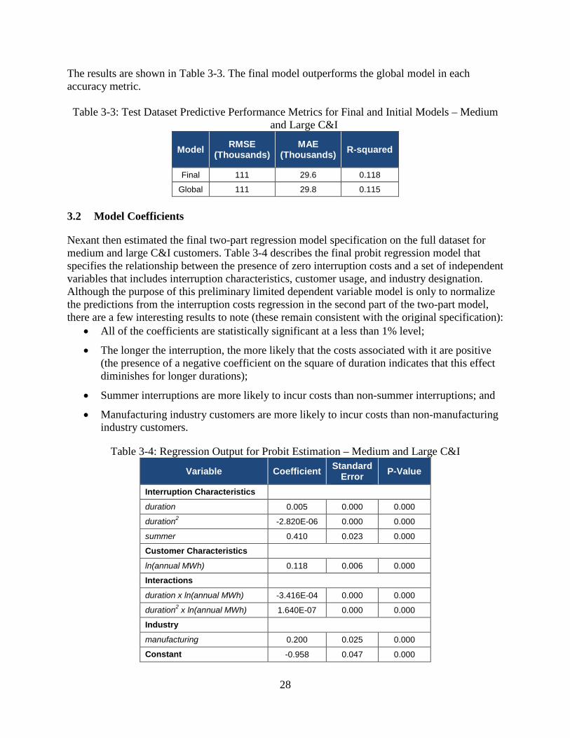
The results are shown in Table 3-3. The final model outperforms the global model in each accuracy metric. Table 3-3: Test Dataset Predictive Performance Metrics for Final and Initial Models – Medium

and Large C&I

Model RMSE (Thousands)

MAE (Thousands) R-squared

Final 111 29.6 0.118

Global 111 29.8 0.115

3.2 Model Coefficients

Nexant then estimated the final two-part regression model specification on the full dataset for medium and large C&I customers. Table 3-4 describes the final probit regression model that specifies the relationship between the presence of zero interruption costs and a set of independent variables that includes interruption characteristics, customer usage, and industry designation. Although the purpose of this preliminary limited dependent variable model is only to normalize the predictions from the interruption costs regression in the second part of the two-part model, there are a few interesting results to note (these remain consistent with the original specification):

• All of the coefficients are statistically significant at a less than 1% level;

• The longer the interruption, the more likely that the costs associated with it are positive (the presence of a negative coefficient on the square of duration indicates that this effect diminishes for longer durations);

• Summer interruptions are more likely to incur costs than non-summer interruptions; and

• Manufacturing industry customers are more likely to incur costs than non-manufacturing industry customers.

Table 3-4: Regression Output for Probit Estimation – Medium and Large C&I

Variable Coefficient Standard Error P-Value

Interruption Characteristics

duration 0.005 0.000 0.000

duration2 -2.820E-06 0.000 0.000

summer 0.410 0.023 0.000

Customer Characteristics

ln(annual MWh) 0.118 0.006 0.000

Interactions

duration x ln(annual MWh) -3.416E-04 0.000 0.000

duration2 x ln(annual MWh) 1.640E-07 0.000 0.000

Industry

manufacturing 0.200 0.025 0.000

Constant -0.958 0.047 0.000

28

Table 3-5 describes the final GLM regression model, which relates the level of interruption costs to customer usage and interruption characteristics as well as industry designation. A few results of note:

• The longer the interruption, the higher the interruption cost;

• Larger customers (in terms of annual MWh usage) incur larger costs for similar interruptions (however, interruption costs increase at a decreasing rate as usage increases);

• Manufacturing industry customers incur larger costs for similar interruptions than equivalent non-manufacturing customers;

• The difference between summer and non-summer interruption costs is statistically insignificant (all other coefficients are statistically significant).

Table 3-5: Customer Regression Output for GLM Estimation – Medium and Large C&I



duration 0.006 0.001 0.000

duration2 -3.260E-06 0.000 0.000

summer 0.113 0.060 0.058


ln(annual MWh) 0.495 0.016 0.000

Interactions

duration x ln(annual MWh) -1.882E-04 0.000 0.047

duration2 x ln(annual MWh) 1.480E-07 0.000 0.028

Industry


Constant 5.292 0.127 0.000

Finally, Table 3-6 shows the average values of the regression inputs for medium and large C&I customers, which are useful for modeling purposes and for assessing marginal effects. Other descriptive statistics are also provided.

Table 3-6: Descriptive Statistics for Regression Inputs – Medium and Large C&I

Variable N Average Minimum 25th Percentile Median 75th

Percentile Maximum


duration 44,328 162 0 60 60 240 1,440

duration2 44,328 82,724 0 3,600 3,600 57,600 2,073,600

summer 44,328 86.5% 0% 100% 100% 100% 100%


ln(annual MWh) 44,328 6.6 3.9 4.9 6.2 7.9 13.9

29


Percentile Maximum

Interactions

duration x ln(annual MWh) 44,328 1,060 0 255 437 1,327 17,064

duration2 x ln(annual MWh) 44,328 530,872 0 14,881 26,250 317,870 24,600,000

Industry

manufacturing 44,328 23.3% 0% 0% 0% 0% 100%

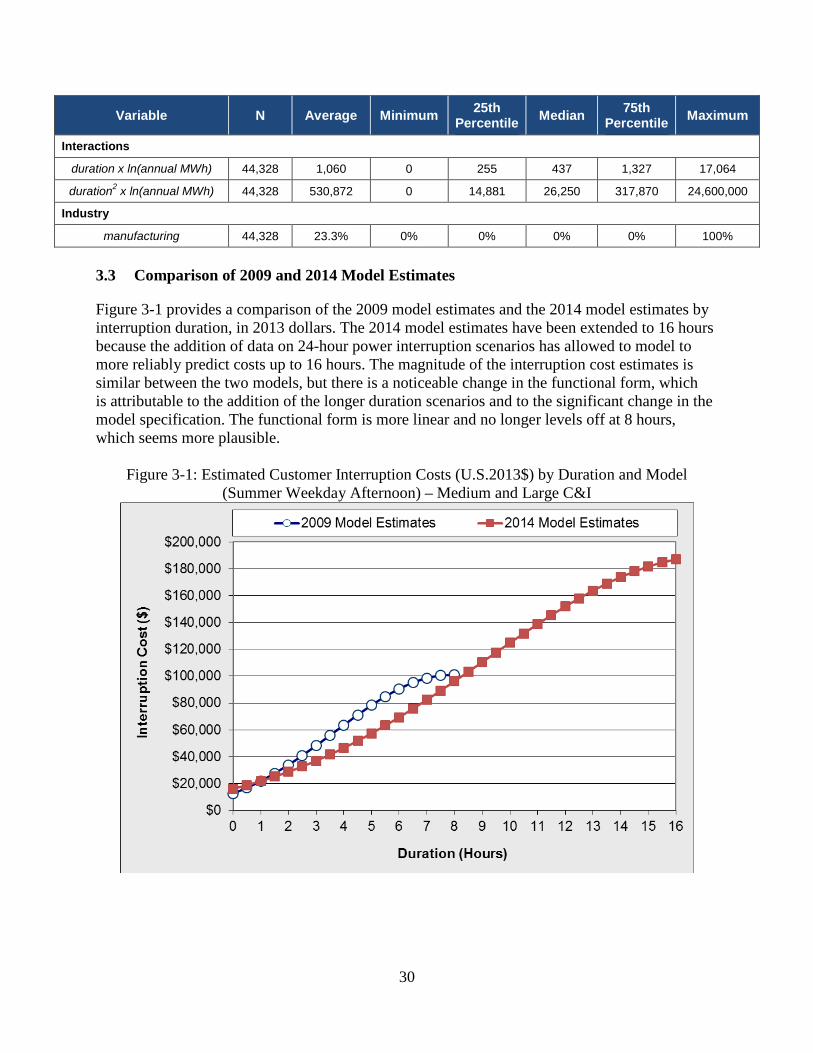
3.3 Comparison of 2009 and 2014 Model Estimates

Figure 3-1 provides a comparison of the 2009 model estimates and the 2014 model estimates by interruption duration, in 2013 dollars. The 2014 model estimates have been extended to 16 hours because the addition of data on 24-hour power interruption scenarios has allowed to model to more reliably predict costs up to 16 hours. The magnitude of the interruption cost estimates is similar between the two models, but there is a noticeable change in the functional form, which is attributable to the addition of the longer duration scenarios and to the significant change in the model specification. The functional form is more linear and no longer levels off at 8 hours, which seems more plausible.

Figure 3-1: Estimated Customer Interruption Costs (U.S.2013$) by Duration and Model (Summer Weekday Afternoon) – Medium and Large C&I

30

3.4 Interruption Cost Estimates and Key Drivers

Table 3-7 shows how medium and large C&I customer interruption costs vary by season. Considering that time of day and day of week were not important factors in the model for medium and large C&I customers, the only temporal variable to consider is season (summer or non-summer). The cost of a summer power interruption is around 21% to 43% higher than a non-summer one, depending on duration (the percent difference lowers as duration increases). Considering that the non-summer time period (October through May) accounts for two-thirds of the year, the weighted-average interruption cost estimate is closer to the non-summer estimate. This weighted-average interruption cost estimate is most appropriate to use for planning purposes, unless the distribution of interruptions by season is known.

Table 3-7: Estimated Customer Interruption Costs (U.S.2013$) by Duration and Timing of Interruption – Medium and Large C&I

Timing of Interruption

% of Hours per Year



Summer 33% $16,172 $18,861 $21,850 $46,546 $96,252 $186,983

Non-summer 67% $11,342 $13,431 $15,781 $35,915 $77,998 $154,731

Weighted Average $12,952 $15,241 $17,804 $39,458 $84,083 $165,482

Based on the weighted-average interruption cost estimate, Table 3-8 provides cost per event (equal to the weighted-average interruption cost), cost per average kW and cost per unserved kWh for medium and large C&I customers. Cost per unserved kWh is relatively high for a momentary interruption because the expected amount of unserved kWh over a 5-minute period is relatively low.

Table 3-8: Cost per Event, Average kW and Unserved kWh – Medium and Large C&I


Momentary 30 Minutes 1 Hour 4 Hours 8 Hours 16 Hours Cost per Event $12,952 $15,241 $17,804 $39,458 $84,083 $165,482



Figure 3-2 shows the medium and large C&I interruption costs in the summer for non-manufacturing and manufacturing customers. As in the 2009 model, interruption costs in the manufacturing sector are relatively high. At all durations, the estimated interruption cost for manufacturing customers is more than double the cost for non-manufacturing customers. This is a key driver to consider for planning purposes – whether the planning area of interest includes medium and large C&I customers with manufacturing facilities that may be particularly sensitive to power interruptions.

31

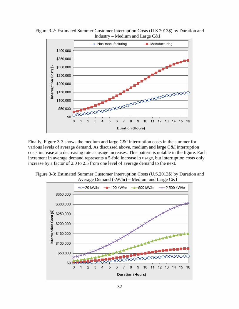
Figure 3-2: Estimated Summer Customer Interruption Costs (U.S.2013$) by Duration and Industry – Medium and Large C&I

Finally, Figure 3-3 shows the medium and large C&I interruption costs in the summer for various levels of average demand. As discussed above, medium and large C&I interruption costs increase at a decreasing rate as usage increases. This pattern is notable in the figure. Each increment in average demand represents a 5-fold increase in usage, but interruption costs only increase by a factor of 2.0 to 2.5 from one level of average demand to the next.

Figure 3-3: Estimated Summer Customer Interruption Costs (U.S.2013$) by Duration and Average Demand (kW/hr) – Medium and Large C&I

32

4. Small C&I Results

This section summarizes the results of the model selection process and provides the model coefficients for small C&I customers, which are C&I customers with annual usage of less than 50,000 kWh. 4.1 Final Model Selection

The global model for small C&I customers was identical to that for the medium and large C&I customers. Refer to Section 3.1 above for a discussion of the global model specification. The global model was successfully parsed down to only key variables. In selecting among variables, categorical variables were not treated as a set (either all or none removed), but rather each binary variable was removed one at a time. This allowed for a particularly important category to remain, while others that might have had a smaller effect were no longer represented. Table 4-1 shows the results of each step in the process. Each iteration represents the exclusion of a variable from the global model, and the variable listed is the one that, when excluded, produces the model with the best performance across various metrics in out-of-sample tests. The model’s value and rank (relative to the other possible exclusions) in the metrics is listed, along with its overall rank, which is an average of the individual ranks. Note that iteration zero represents the global model alone, so some metrics that are only meaningful when compared with other models, such as ranks and AICs, are not listed. The highlighted row shows the final exclusion that was made; the rows that follow show the variables that remain in the final model. Ultimately, interruption costs for small C&I customers can be estimated relatively accurately with variables representing customer usage and interruption duration, along with some binary variables for customer characteristics and interruption timing. Considering how difficult it can be for ICE Calculator users to find information for some of the 12 excluded variables (especially for small C&I customers), this final model will be much easier to use.

33

Table 4-1: Excluded Variables and Relevant Metrics from Backwards Stepwise Selection Process – Small C&I

The final model for small C&I customers is shown below:

𝐼𝐼𝐼𝐼𝐼𝐼𝐼𝐼𝐼𝐼𝐼𝐼𝐼𝐼𝐼𝐼𝐼𝐼𝐼𝐼𝐼𝐼𝐼𝐼 𝐶𝐶𝐼𝐼𝐶𝐶𝐼𝐼 = 𝑓𝑓(ln(𝑎𝑎𝐼𝐼𝐼𝐼𝐼𝐼𝑎𝑎𝑎𝑎 𝑀𝑀𝑀𝑀𝑀𝑀) ,𝑑𝑑𝐼𝐼𝐼𝐼𝑎𝑎𝐼𝐼𝐼𝐼𝐼𝐼𝐼𝐼,𝑑𝑑𝐼𝐼𝐼𝐼𝑎𝑎𝐼𝐼𝐼𝐼𝐼𝐼𝐼𝐼2, 𝐶𝐶𝐼𝐼𝑠𝑠𝑠𝑠𝐼𝐼𝐼𝐼, 𝐼𝐼𝐼𝐼𝑑𝑑𝐼𝐼𝐶𝐶𝐼𝐼𝐼𝐼𝑤𝑤,𝑏𝑏𝑎𝑎𝑏𝑏𝑤𝑤𝐼𝐼𝐼𝐼 𝐼𝐼𝑒𝑒𝐼𝐼𝐼𝐼𝐼𝐼𝑠𝑠𝐼𝐼𝐼𝐼𝐼𝐼, 𝐼𝐼𝐼𝐼𝑠𝑠𝐼𝐼 𝐼𝐼𝑓𝑓 𝑑𝑑𝑎𝑎𝑤𝑤)

Industry, backup equipment and time of day are the only categorical variables remaining, and many of the categories were removed. Note that as categories are removed, they are relegated to the reference category, so for example the construction binary variable should now be interpreted as the average impact on interruption cost associated with being in the construction industry, relative to all industries other than manufacturing, which is the only other industry that was retained as a binary variable. The categories that remain in the final model are shown in Table 4-2 below.

Table 4-2: Breakdown of Categorical Variables Featured in Final Model – Small C&I Variable Categories industry Other; Construction; Manufacturing

backup equipment None; Backup Gen or Power Conditioning; Backup Gen and Power Conditioning

time of day Other (5 PM to 6 AM); Morning (6 AM to 12 PM); Afternoon (12 to 5 PM)

Value (Thousands)

RankValue (Thousands)

Rank Value Rank

Probit Value

(Thousands)

GLM Value

(Thousands)

Rank

0 - 6.17 - 1.95 - 0.044 - - - - -

1 transportation, comunication & utilities 6.16 1 1.94 2 0.048 1 30.6 245 8.0 3.0

2 mining 6.16 1 1.94 1 0.049 1 30.6 245 7.0 2.5

3 warning 6.16 1 1.94 3 0.049 1 30.6 245 4.5 2.4

4 evening 6.16 1 1.94 2 0.049 2 30.6 245 4.0 2.3

5 duration 2 x ln(annual MWh) 6.16 1 1.94 3 0.049 2 30.6 245 3.0 2.3

6 finance, insurance & real estate 6.16 2 1.94 4 0.049 2 30.7 245 5.5 3.4

7 unknown industry 6.16 5 1.94 2 0.049 2 30.7 245 5.5 3.6

8 duration x ln(annual MWh) 6.16 3 1.94 2 0.049 2 30.7 245 1.5 2.1

9 public administration 6.16 2 1.94 3 0.049 4 30.7 245 2.0 2.8

10 weekday 6.16 2 1.94 3 0.048 3 30.7 245 3.5 2.9

11 wholesale & retail trade 6.16 1 1.94 1 0.049 1 30.9 245 7.5 2.6

12 services 6.16 2 1.94 1 0.049 3 30.9 245 2.0 2.0

13 morning 6.16 2 1.95 2 0.048 2 31.4 245 4.5 2.6

14 afternoon 6.16 1 1.95 2 0.048 1 31.5 245 3.0 1.8

15 summer 6.17 1 1.95 1 0.047 1 31.8 245 4.5 1.9

16 ln(annual MWh) 6.17 1 1.96 3 0.045 1 32.0 245 3.0 2.0

17 backupgen and power conditioning 6.19 2 1.97 1 0.041 1 32.1 246 2.5 1.6

18 backupgen or power conditioning 6.20 1 1.98 1 0.036 1 32.1 246 2.0 1.3

19 manufacturing 6.22 1 2.00 2 0.029 1 32.1 246 1.5 1.4

20 construction 6.24 1 2.01 1 0.023 1 32.2 247 1.0 1.0

21 duration 2 6.52 1 2.16 1 -0.089 1 32.8 248 1.0 1.0

22 duration 6.32 1 2.13 1 -0.001 1 34.2 251 1.0 1.0

Overall RankIteration Excluded Variable

RMSE MAE R2 AIC

34

To confirm that the selection process did not produce an overfitted model, and to estimate the predictive performance of the final model when evaluated on unseen data, Nexant evaluated the final model against the global model using the test dataset, which is the 10% of data that was held out from the backwards stepwise selection process. Both models were fitted to the remaining data, and then the test dataset was used to evaluate their predictive performance. The results are shown in Table 4-3. Note that while the global model outperforms the final model in each metric, the differences between the values are very small. The final model offers a much simpler solution with comparable performance to the global model. Table 4-3: Test Dataset Predictive Performance Metrics for Final and Initial Models – Small C&I

Model RMSE (Thousands)

MAE (Thousands) R-squared

Final 5.50 1.82 0.045

Global 5.49 1.82 0.048


Nexant then estimated the final two-part regression model specification on the full dataset for residential customers. Table 4-4 describes the final probit regression model that specifies the relationship between the presence of zero interruption costs and a set of independent variables that includes interruption characteristics, customer characteristics, and industry designation. Although the purpose of this preliminary limited dependent variable model is only to normalize the predictions from the interruption costs regression in the second part of the two-part model, there are a few interesting results to note (these remain consistent with the original specification):


• The longer the interruption, the more likely that the costs associated with it are positive (the presence of a negative coefficient on the square of duration indicates that this effect diminishes for longer durations);

• Summer interruptions are more likely to incur costs than non-summer interruptions;

• Afternoon interruptions are more likely to incur costs than any other time of day; and

• Manufacturing and construction customers are more likely to incur costs than customers in other industries.

Table 4-4: Customer Regression Output for Probit Estimation – Small C&I



duration 0.003 0.000 0.000

duration2 -1.780E-06 0.000 0.000

summer 0.215 0.030 0.000

morning 0.537 0.022 0.000

afternoon 0.664 0.029 0.000

35



ln(annual MWh) 0.124 0.013 0.000

backupgen or power conditioning 0.082 0.025 0.001

backupgen and power conditioning 0.272 0.059 0.000

Industry

construction 0.261 0.054 0.000


Constant -1.332 0.048 0.000

Table 4-5 describes the final GLM regression model, which relates the level of interruption costs to customer and interruption characteristics as well as industry designation. A few results of note:


• Larger customers (in terms of annual MWh usage) incur larger costs for similar interruptions (however, interruption costs increase at a decreasing rate as usage increases);

• Manufacturing and construction industry customers incur larger costs for similar interruptions than equivalent customers in other industries; and

• Summer interruptions incur lower interruption costs than other times of the year.

Table 4-5: Customer Regression Output for GLM Estimation – Small C&I



duration 0.004 0.000 0.000

duration2 -2.160E-06 0.000 0.000

summer -0.384 0.073 0.000

morning -0.057 0.070 0.413

afternoon -0.032 0.083 0.701


ln(annual MWh) 0.069 0.035 0.046

backupgen or power conditioning 0.308 0.058 0.000

backupgen and power conditioning 0.538 0.129 0.000

Industry

construction 0.786 0.153 0.000


Constant 7.000 0.135 0.000

36

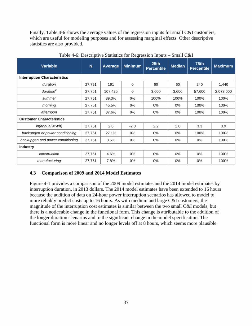
Finally, Table 4-6 shows the average values of the regression inputs for small C&I customers, which are useful for modeling purposes and for assessing marginal effects. Other descriptive statistics are also provided.

Table 4-6: Descriptive Statistics for Regression Inputs – Small C&I


Percentile Maximum


duration 27,751 191 0 60 60 240 1,440

duration2 27,751 107,425 0 3,600 3,600 57,600 2,073,600

summer 27,751 89.3% 0% 100% 100% 100% 100%

morning 27,751 45.5% 0% 0% 0% 100% 100%

afternoon 27,751 37.6% 0% 0% 0% 100% 100%


ln(annual MWh) 27,751 2.6 -2.0 2.2 2.8 3.3 3.9

backupgen or power conditioning 27,751 27.1% 0% 0% 0% 100% 100%

backupgen and power conditioning 27,751 3.5% 0% 0% 0% 0% 100%

Industry

construction 27,751 4.6% 0% 0% 0% 0% 100%

manufacturing 27,751 7.8% 0% 0% 0% 0% 100%


Figure 4-1 provides a comparison of the 2009 model estimates and the 2014 model estimates by interruption duration, in 2013 dollars. The 2014 model estimates have been extended to 16 hours because the addition of data on 24-hour power interruption scenarios has allowed to model to more reliably predict costs up to 16 hours. As with medium and large C&I customers, the magnitude of the interruption cost estimates is similar between the two small C&I models, but there is a noticeable change in the functional form. This change is attributable to the addition of the longer duration scenarios and to the significant change in the model specification. The functional form is more linear and no longer levels off at 8 hours, which seems more plausible.

37

Figure 4-1: Estimated Customer Interruption Costs (U.S.2013$) by Duration and Model (Summer Weekday Afternoon) – Small C&I


Table 4-7 shows how small C&I customer interruption costs vary by season and time of day. The cost of a summer power interruption is around 9% to 30% lower than a non-summer one, depending on duration, season, and time of day. Interestingly, this is opposite the pattern of medium and large C&I customers, which experience higher interruption costs during the summer. As for how interruption costs vary by time of day, costs are highest in the afternoon and are similarly high in the morning. In the evening and nighttime, small C&I interruption costs are substantially lower, which makes sense given that small businesses typically operate during daytime hours. Considering that the evening/night time period (5 PM to 6 AM) accounts for a majority of the hours of the day, the weighted-average interruption cost estimate is closer to the evening/night estimates. This weighted-average interruption cost estimate is most appropriate to use for planning purposes, unless the distribution of interruptions by season and time of day is known.

38

Table 4-7: Estimated Customer Interruption Costs (U.S.2013$) by Duration and Timing of Interruption – Small C&I


Hours per Year



Summer Morning 8% $461 $569 $692 $1,798 $4,073 $7,409

Summer Afternoon 7% $527 $645 $780 $1,954 $4,313 $7,737

Summer Evening/Night 18% $272 $349 $440 $1,357 $3,518 $6,916

Non-summer Morning 17% $549 $687 $848 $2,350 $5,592 $10,452

Non-summer Afternoon 14% $640 $794 $972 $2,590 $5,980 $10,992

Non-summer Evening/Night 36% $298 $388 $497 $1,656 $4,577 $9,367

Weighted Average $412 $520 $647 $1,880 $4,690 $9,055

Based on the weighted-average interruption cost estimate, Table 4-8 provides cost per event (equal to the weighted-average interruption cost), cost per average kW, and cost per unserved kWh for small C&I customers. Cost per unserved kWh is relatively high for a momentary interruption because the expected amount of unserved kWh over a 5-minute period is relatively low.

Table 4-8: Cost per Event, Average kW and Unserved kWh – Small C&I



Cost per Event $412 $520 $647 $1,880 $4,690 $9,055

Cost per Average kW $187.9 $237.0 $295.0 $857.1 $2,138.1 $4,128.3

Cost per Unserved kWh $2,254.6 $474.1 $295.0 $214.3 $267.3 $258.0

Figure 4-2 shows the small C&I interruption costs in the summer afternoon by industry. As in the 2009 model, interruption costs in the manufacturing and construction sectors are relatively high. At all durations, the estimated interruption cost for manufacturing and construction customers is around double or more the cost for customers in other industries. As in the medium and large C&I customer class, this is a key driver to consider for planning purposes – whether the planning area of interest includes small C&I customers with manufacturing or construction facilities that may be particularly sensitive to power interruptions.

39

Figure 4-2: Estimated Summer Afternoon Customer Interruption Costs (U.S.2013$) by Duration and Industry – Small C&I

Finally, Figure 4-3 shows the small C&I interruption costs in the summer afternoon for various levels of average demand. Small C&I interruption costs are not highly sensitive to the average demand of a customer. In the figure, each increment in average demand represents a 2-fold increase in usage, but interruption costs only increase by around 10% from one level of average demand to the next. Figure 4-3: Estimated Summer Afternoon Customer Interruption Costs (U.S.2013$) by Duration

and Average Demand (kW/hr) – Small C&I

40

5. Residential Results

This section summarizes the results of the model selection process and provides the model coefficients for residential customers. 5.1 Final Model Selection

The global model for residential customers is shown below: Interruption Cost = f(ln(annual MWh), duration, duration2, household income, medical equip., backup generation, summer, weekday, outage in last 12 months, # residents 0-6, # residents 7-18, # residents 19-24, # residents 25-49, # residents 50-64, # residents over 64, time of day, housing) Interruption cost is expressed as a function of various explanatory variables. Note that the dependent variables differ between the probit and GLM models; hence the above equation expresses the two-part model in its most general form. Time of day and housing are categorical variables, and their respective categories are shown in Table 5-1 below. As is typical in indicatory coding, the first category within each categorical variable is not included explicitly as a binary variable, but rather serves as a reference category.

Table 5-1: Breakdown of Categorical Variables Featured in Global Model – Residential Variable Categories

time of day Morning (6 AM to 12 PM); Afternoon (12 to 5 PM); Evening (5 to 10 PM); Late Evening/Early Morning

housing Detached; Attached; Apartment/Condo; Mobile; Manufactured; Unknown

The global model was successfully parsed down to only key variables. In selecting among variables, categorical variables were not treated as a set (either all or none removed), but rather each binary variable was removed one at a time. This allowed for a particularly important category to remain, while others that might have had a smaller effect were no longer represented. Table 5-2 shows the results of each step in the process. Each iteration represents the exclusion of a variable from the global model, and the variable listed is the one that, when excluded, produces the model with the best performance across various metrics in out-of-sample tests. The model’s value and rank (relative to the other possible exclusions) in the metrics is listed, along with its overall rank, which is an average of the individual ranks. Note that iteration zero represents the global model alone, so some metrics that are only meaningful when compared with other models, such as ranks and AICs, are not listed. The highlighted row shows the final exclusion that was made; the rows that follow show the variables that remain in the final model. Ultimately, interruption costs for residential customers can be estimated relatively accurately with variables representing customer usage, household income, and interruption duration, along with some binary variables for interruption timing. A few of the 16 excluded variables show a minor improvement in predictive accuracy, but considering how difficult it can be for ICE Calculator users to find information for some of those inputs, this minor improvement in predictive accuracy was not sufficient to justify keeping those variables in the final model.

41

Table 5-2: Excluded Variables and Relevant Metrics from Backwards Stepwise Selection Process – Residential

The final model for residential customers is shown below: Interruption Cost = f(ln(annual MWh), duration, duration2, household income, summer, time of day) To confirm that the selection process did not produce an over-fitted model, and to estimate the predictive performance of the final model when evaluated on unseen data, Nexant evaluated the final model against the global model using the test dataset, which is the 10% of data that was held out from the backwards stepwise selection process. Both models were fitted to the remaining data, and then the test dataset was used to evaluate their predictive performance. The results are shown in Table 5-3. Note that while the global model outperforms the final model in each metric, the differences between the values are very small. The final model offers a much simpler solution with comparable performance to the global model.

Value Rank Value Rank Value Rank

Probit Value (Thousands)

GLM Value

(Thousands)

Rank

0 - 16.6 - 8.50 - 0.145 - - - - -

1 late evening/early morning 16.5 1 8.49 1 0.147 1 37.3 126 9.5 3.1

2 mobile housing 16.5 3 8.48 2 0.148 3 37.3 126 3.5 2.9

3 outage in last 12 months 16.5 1 8.48 1 0.149 1 37.3 126 9.5 3.1

4 # residents 7-18 years old 16.5 1 8.48 5 0.149 1 37.3 126 6.0 3.3



7 manufactured housing 16.5 2 8.48 2 0.149 2 37.3 126 4.0 2.5

8 weekday 16.5 1 8.48 2 0.149 1 37.3 126 5.5 2.4

9 attached housing 16.5 1 8.48 1 0.149 1 37.4 126 5.5 2.1

10 apartment/condo 16.5 3 8.48 2 0.149 3 37.4 126 1.0 2.3


12 backup generation 16.5 1 8.48 1 0.149 1 37.4 126 4.0 1.8


14 unknown housing 16.5 2 8.49 1 0.148 2 37.4 126 1.5 1.6

15 medical equipment 16.5 1 8.49 2 0.148 1 37.5 126 2.5 1.6

16 # residents 65 and over 16.6 1 8.49 1 0.146 1 37.5 126 2.5 1.4

17 household income 16.6 1 8.53 1 0.140 1 37.5 127 2.5 1.4

18 evening, 5 pm to 8 pm 16.7 1 8.61 2 0.133 1 38.7 127 3.0 1.8

19 afternoon, 12 noon to 4 pm 16.7 1 8.63 1 0.127 1 38.9 127 2.0 1.3

20 summer 16.8 1 8.71 1 0.119 1 39.7 127 2.0 1.3

21 ln(annual MWh) 17.0 1 8.82 1 0.098 1 39.7 128 1.5 1.1

22 duration 2 17.3 1 8.95 1 0.072 1 39.9 128 1.0 1.0

23 duration 17.9 1 9.44 1 0.000 1 41.6 130 1.0 1.0

Iteration Excluded Variable Overall Rank

RMSE MAE R2 AIC

42

Table 5-3: Test Dataset Predictive Performance Metrics for Final and Initial Models – Residential

Model RMSE MAE R-squared Final 17.5 8.34 0.148

Global 17.3 8.28 0.165


Nexant then estimated the final two-part regression model specification on the full dataset for residential customers. Table 5-4 describes the final probit regression model that specifies the relationship between the presence of zero interruption costs and a set of independent variables that includes interruption characteristics and customer characteristics. Although the purpose of this preliminary limited dependent variable model is only to normalize the predictions from the interruption costs regression in the second part of the two-part model, there are a few interesting results to note (these remain consistent with the original specification):


• The longer the interruption, the more likely that the costs are positive (the presence of a negative coefficient on the square of duration indicates that this effect diminishes for longer durations);

• Customers are less likely to have a positive cost for an afternoon or an evening interruption versus any other time of day.

Table 5-4: Regression Output for Probit Estimation – Residential



duration 0.003 0.000 0.000

duration2 -1.130E-06 0.000 0.000

summer 0.541 0.019 0.000

afternoon -0.266 0.026 0.000

evening -0.755 0.024 0.000


ln(annual MWh) 0.038 0.018 0.035

household income 9.660E-07 0.000 0.004

Constant -0.266 0.051 0.000

Table 5-5 describes the final GLM regression model which relates the level of interruption costs to customer and interruption characteristics. A few results of note:



43

• Customers have lower interruption costs for afternoon and evening interruptions than for those that occur at other times of day;

• Customers experience higher costs for summer interruptions than for non-summer interruptions; and

• Larger customers (in terms of annual MWh usage) have a higher cost for similar interruptions than otherwise equivalent, smaller customers.

Table 5-5: Regression Output for GLM Estimation – Residential



duration 0.002 0.000 0.000

duration2 -9.450E-07 0.000 0.000

summer 0.161 0.029 0.000

afternoon -0.282 0.041 0.000

evening -0.095 0.047 0.044


ln(annual MWh) 0.249 0.028 0.000

household income 1.850E-06 0.000 0.000

Constant 1.379 0.080 0.000

Finally, Table 5-6 shows the average values of the regression inputs for residential customers, which are useful for modeling purposes and for assessing marginal effects. Other descriptive statistics are also provided.

Table 5-6: Descriptive Statistics for Regression Inputs – Residential


Percentile Maximum


duration 34,212 168 0 60 60 240 1,440

duration2 34,212 82,198 0 3,600 3,600 57,600 2,073,600

summer 34,212 73.4% 0% 0% 100% 100% 100%

afternoon 34,212 48.8% 0% 0% 0% 100% 100%

evening 34,212 29.1% 0% 0% 0% 100% 100%


ln(annual MWh) 34,212 2.4 0.3 1.9 2.4 2.9 4.4

household income 34,212 69,243 5,076 36,846 63,445 97,618 173,611

44


Figure 5-1 provides a comparison of the 2009 model estimates and the 2014 model estimates by interruption duration, in 2013 dollars. The 2014 model estimates have been extended to 16 hours because the addition of data on 24-hour power interruption scenarios has allowed to model to more reliably predict costs up to 16 hours. As with C&I customers, the magnitude of the interruption cost estimates is similar between the two small C&I models, but there is a noticeable change in the functional form. This change is attributable to the addition of the longer duration scenarios and to the significant change in the model specification. The functional form is more linear and no longer levels off at 8 hours, which seems more plausible.

Figure 5-1: Estimated Customer Interruption Costs (U.S.2013$) by Duration and Model (Summer Weekday Afternoon) – Residential


Table 5-7 shows how residential customer interruption costs vary by season and time of day. The cost of a summer power interruption is substantially higher than a non-summer one, for all durations, seasons, and times of day. As for how interruption costs vary by time of day, costs are highest in the morning and night (10 PM to 12 noon). The weighted-average interruption cost estimate is most appropriate to use for planning purposes, unless the distribution of interruptions by season and time of day is known.

45

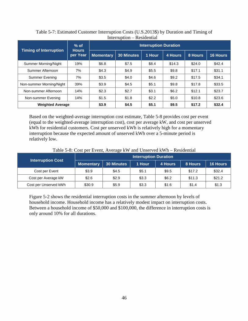
Table 5-7: Estimated Customer Interruption Costs (U.S.2013$) by Duration and Timing of Interruption – Residential


Hours per Year



Summer Morning/Night 19% $6.8 $7.5 $8.4 $14.3 $24.0 $42.4

Summer Afternoon 7% $4.3 $4.9 $5.5 $9.8 $17.1 $31.1

Summer Evening 7% $3.5 $4.0 $4.6 $9.2 $17.5 $34.1

Non-summer Morning/Night 39% $3.9 $4.5 $5.1 $9.8 $17.8 $33.5

Non-summer Afternoon 14% $2.3 $2.7 $3.1 $6.2 $12.1 $23.7

Non-summer Evening 14% $1.5 $1.8 $2.2 $5.0 $10.8 $23.6

Weighted Average $3.9 $4.5 $5.1 $9.5 $17.2 $32.4

Based on the weighted-average interruption cost estimate, Table 5-8 provides cost per event (equal to the weighted-average interruption cost), cost per average kW, and cost per unserved kWh for residential customers. Cost per unserved kWh is relatively high for a momentary interruption because the expected amount of unserved kWh over a 5-minute period is relatively low.

Table 5-8: Cost per Event, Average kW and Unserved kWh – Residential


Momentary 30 Minutes 1 Hour 4 Hours 8 Hours 16 Hours Cost per Event $3.9 $4.5 $5.1 $9.5 $17.2 $32.4



Figure 5-2 shows the residential interruption costs in the summer afternoon by levels of household income. Household income has a relatively modest impact on interruption costs. Between a household income of $50,000 and $100,000, the difference in interruption costs is only around 10% for all durations.

46

Figure 5-2: Estimated Summer Afternoon Customer Interruption Costs (U.S.2013$) by Duration and Household Income – Residential

Finally, Figure 5-3 shows the residential interruption costs in the summer afternoon for various levels of average demand. Residential interruption costs are not highly sensitive to the average demand of a customer. In the figure, each increment in average demand represents a 2-fold increase in usage, but interruption costs only increase by around 20% from one level of average demand to the next. Figure 5-3: Estimated Summer Afternoon Customer Interruption Costs (U.S.2013$) by Duration

and Average Demand (kW/hr) – Residential

47

6. Study Limitations

As in the 2009 study, there are limitations to how the data from this meta-analysis should be used. It is important to fully understand these limitations, so they are further described in this section. First, certain very important variables in the data are confounded among the studies we examined. In particular, region of the country and year of the study are correlated in such a way that it is impossible to separate the effects of these two variables on customer interruption costs. Thus, for example, it is unclear whether the higher interruption cost values for the southwest are purely the result of the hot summer climate in that region or whether those costs are higher in part because of the particular economic and market conditions that prevailed during the year when the study for that region was done. The same logic applies to the 2012 west study, which was the only survey to include power interruption scenarios of more than 12 hours, which makes it difficult to separate the effect of region and year from the effect of the relatively long interruption duration. There is further correlation between regions and scenario characteristics. The sponsors of the interruption cost studies were generally interested in measuring interruption costs for conditions that were important for planning for their specific systems. As a result, interruption conditions described in the surveys for a given region tended to focus on periods of time when interruptions were more problematic for that region. Unfortunately, the time periods when the chance of interruptions is greatest are not identical for all sponsors of the studies we relied upon, so interruption scenario characteristics tended to be different in different regions. Fortunately, most of the studies we examined included a summer afternoon interruption, so we could compare that condition among studies. A further limitation of our research is that the surveys that formed the basis of the studies we examined were limited to certain parts of the country. No data were available from the northeast/mid-Atlantic region, and limited data were available for cities along the Great Lakes. The absence of interruption cost information for the northeast/mid-Atlantic region is particularly troublesome because of the unique population density and economic intensity of that region. It is unknown whether, when weather and customer compositions are controlled, the average interruption costs from this region are different than those in other parts of the country. Another caveat is that around half of the data from the meta-database is from surveys that are 15 or more years old. Although the intertemporal analysis in the 2009 study showed that interruption costs have not changed significantly over time, the outdated vintage of the data presents concerns that, in addition to the limitations above, underscore the need for a coordinated, nationwide effort that collects interruption cost estimates for many regions and utilities simultaneously, using a consistent survey design and data collection method. Finally, as described in Section 1, although the revised model is able to estimate costs for interruptions lasting longer than 8 hours, it is important to note that the estimates in this report are not appropriate for resiliency planning. This meta-study focuses on the direct costs that customers experience as a result of relatively short power interruptions of up to 24 hours at most. In fact, the final models and results that are presented in Sections 3 through 5 truncate the estimates at 16 hours, due to the relatively few number of observations beyond 12 hours

48

(scenarios of more than 12 hours account for around 2% to 3% of observations for all customer classes). For resiliency considerations that involve planning for long duration power interruptions of 24 hours or more, the nature of costs change and the indirect, spillover effects to the greater economy must be considered.12 These factors are not captured in this meta-analysis.


49

updated value of service reliability estimates for ...emp.lbl.gov/sites/all/files/lbnl-6941e.pdf ·...

Documents