uplink system performance of lte-advanced relay ... · pdf filelte-advanced relay deployments...

Uplink System Performance of LTE-Advanced Relay Deployments in Different Propagation Environments Ömer Bulakci1,2, Abdallah Bou Saleh2, Simone Redana1, and Jyri Hämäläinen2

1. Nokia Siemens Networks, NSN-Research, Radio Systems, Munich, Germany 2. Aalto University School of Electrical Engineering, Helsinki, Finland (formerly Helsinki University of Technology-HUT)

17. VDE/ITG Workshop on 09.05.2012

-Mobile Communications-

Ömer Bulakci 2

• Goal

• Uplink Radio Resource Management Strategies Power Control Resource Sharing & Co-scheduling Relay Cell Range Extension

• Joint Optimization: Taguchi’s Method

• Uplink Performance Evaluation Propagation Environments 3GPP Case 1 – ISD 500m 3GPP Case 3 – ISD 1732m

• Conclusions

Content

Ömer Bulakci 3

Goal Analyze uplink system performance of LTE-A Relay Deployments

Balance the load between RN cells and macrocells

Relax downlink-uplink imbalance

Joint Optimization of RRM strategies

Different Propagation Environments

Optimize resource splits between macro-UEs and RNs, and between relay-UEs

Enable a fast adaptation to dynamic system conditions via co-scheduling

Content • Goal




• Conclusions

5 Ömer Bulakci

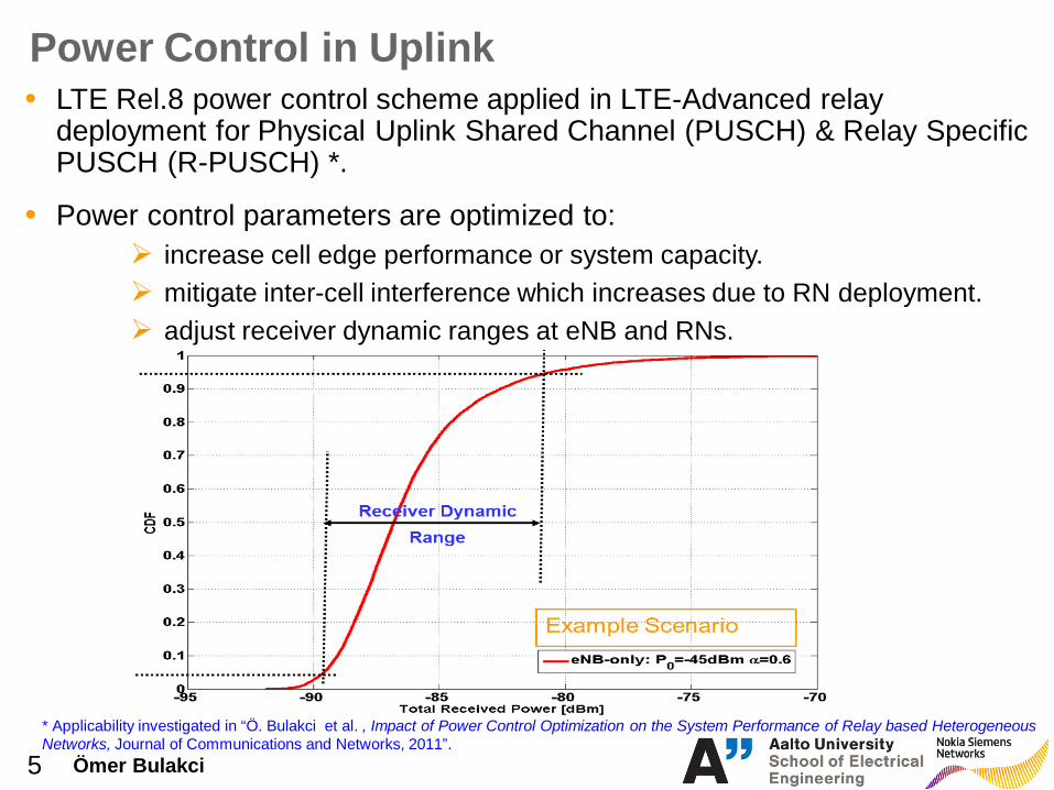
Power Control in Uplink • LTE Rel.8 power control scheme applied in LTE-Advanced relay

deployment for Physical Uplink Shared Channel (PUSCH) & Relay Specific PUSCH (R-PUSCH) *. • Power control parameters are optimized to:

increase cell edge performance or system capacity. mitigate inter-cell interference which increases due to RN deployment. adjust receiver dynamic ranges at eNB and RNs.

* Applicability investigated in “Ö. Bulakci et al. , Impact of Power Control Optimization on the System Performance of Relay based Heterogeneous Networks, Journal of Communications and Networks, 2011”.

6 Ömer Bulakci

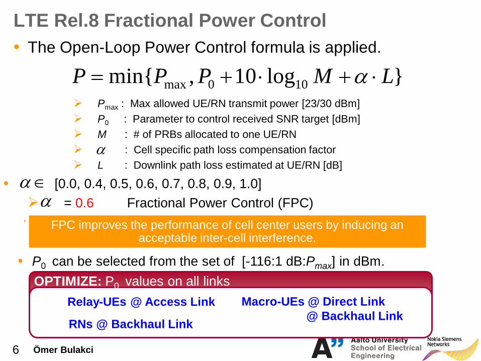
OPTIMIZE: P0 values on all links

LTE Rel.8 Fractional Power Control • The Open-Loop Power Control formula is applied.

}log10,min{ 100max LMPPP ⋅+⋅+= α

• P0 can be selected from the set of [-116:1 dB:Pmax] in dBm.

Pmax : Max allowed UE/RN transmit power [23/30 dBm] P0 : Parameter to control received SNR target [dBm] M : # of PRBs allocated to one UE/RN : Cell specific path loss compensation factor L : Downlink path loss estimated at UE/RN [dB]

• [0.0, 0.4, 0.5, 0.6, 0.7, 0.8, 0.9, 1.0] = 0.6 Fractional Power Control (FPC) ∈αα

FPC improves the performance of cell center users by inducing an acceptable inter-cell interference.

α

Relay-UEs @ Access Link

RNs @ Backhaul Link

Macro-UEs @ Direct Link @ Backhaul Link

Content • Goal




• Conclusions

Ömer Bulakci 8

Resource Sharing & Co-scheduling * Max-Min Fairness

100

e2e 20

e2e 20+20 = 40

e2e: 20+20 = 40

100 instantaneous

80 instantaneous

20 instantaneous

Number of attached relay-UEs

3/6*all PRB

2/6*all PRB

1/6*all PRB

Hop-optimization

Model

f

t RNs Over-provisioned Un Subframes Macro-UEs (Un)

Macro-UEs are scheduled with

RNs Prop. to # of macro-UEs

Advantages: Flexible & Efficient Resource Allocation. Higher SINR values for co-scheduled macro-UEs.

OPTIMIZE: # of Backhaul Subframes

Macro-UEs (Uu)

* “Ö. Bulakci et al. , Radio Resource Management in LTE-Advanced Relay Networks: Optimization Methods and Uplink Performance Evaluation, Wiley ETT, 2012”.

Content • Goal




• Conclusions

Ömer Bulakci 10

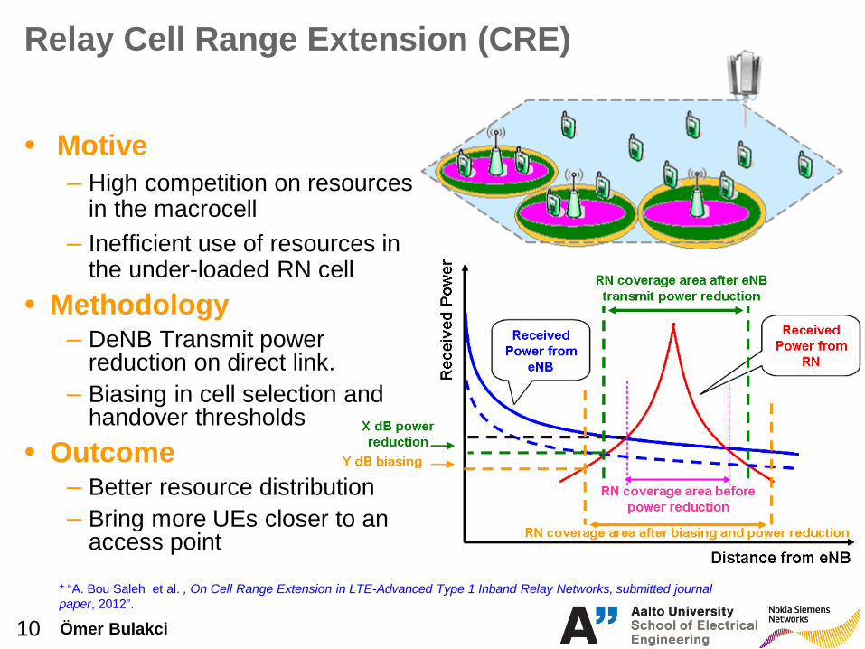
Relay Cell Range Extension (CRE)

• Motive – High competition on resources

in the macrocell – Inefficient use of resources in

the under-loaded RN cell • Methodology

– DeNB Transmit power reduction on direct link.

– Biasing in cell selection and handover thresholds

• Outcome – Better resource distribution – Bring more UEs closer to an

access point

* “A. Bou Saleh et al. , On Cell Range Extension in LTE-Advanced Type 1 Inband Relay Networks, submitted journal paper, 2012”.

Ömer Bulakci 11

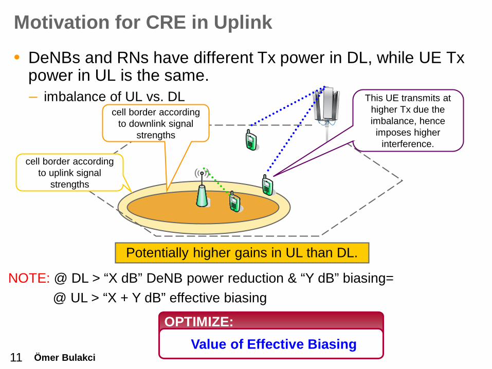
NOTE: @ DL > “X dB” DeNB power reduction & “Y dB” biasing= @ UL > “X + Y dB” effective biasing

Motivation for CRE in Uplink

• DeNBs and RNs have different Tx power in DL, while UE Tx power in UL is the same. – imbalance of UL vs. DL

Potentially higher gains in UL than DL.

cell border according to downlink signal

strengths

cell border according to uplink signal

strengths

This UE transmits at higher Tx due the imbalance, hence imposes higher

interference.

OPTIMIZE: Value of Effective Biasing

Content • Goal




• Conclusions

13 Ömer Bulakci

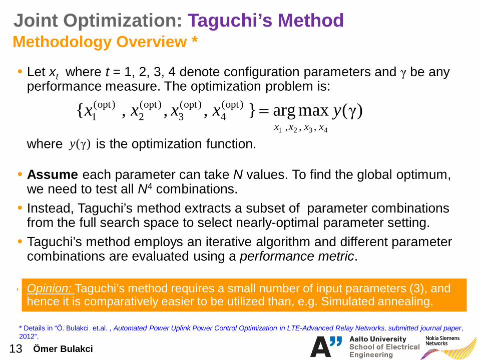
Joint Optimization: Taguchi’s Method Methodology Overview *

• Let xt where t = 1, 2, 3, 4 denote configuration parameters and γ be any performance measure. The optimization problem is:

)γ(maxarg},,,{4321 ,,,

)opt(4

)opt(3

)opt(2

)opt(1 yxxxx

xxxx=

where is the optimization function. )γ(y

• Assume each parameter can take N values. To find the global optimum, we need to test all N4 combinations.

• Instead, Taguchi’s method extracts a subset of parameter combinations from the full search space to select nearly-optimal parameter setting.

• Taguchi’s method employs an iterative algorithm and different parameter combinations are evaluated using a performance metric.

Opinion: Taguchi’s method requires a small number of input parameters (3), and hence it is comparatively easier to be utilized than, e.g. Simulated annealing.

* Details in “Ö. Bulakci et.al. , Automated Power Uplink Power Control Optimization in LTE-Advanced Relay Networks, submitted journal paper, 2012”.

14 Ömer Bulakci

Performance Metric

• Conventional performance metrics: 5%-ile, 50%-ile UE TP CDF levels.

)100

(F 1%

qΓy sq−==

Inverse UE TP CDF Percentile

Conventional Performance Metrics

∑ =

⋅+⋅+⋅== 3

1

%50

%503

%25

%252

%5

%51

)( AM

321

j j

w,w,w

w

ΓwΓwΓwΓy κκκ

Normalization w.r.t. eNB-only

Particularly useful for large-ISD scenarios

• In our example, we utilize a new performance metric: weighted arithmetic mean of the conventional metrics.

Weights to set priority

Joint Optimization: Taguchi’s Method

Content • Goal




• Conclusions

Ömer Bulakci 16

Propagation Environments Scenario 1 (Sc1)

Single-slope model

Scenario 2 (Sc2) Scenario 3 (Sc3)

ALL links are NLOS.

)(log10PLPL 100 Rn ⋅⋅+=

DL Rx. Power (No CRE)

Mixed LOS/NLOS on the access link.

NLOS

LOS

PL)NLOS(PrPL)LOS(PrPL⋅

+⋅= Probabilistic

Dual-slope model

Any link can be either LOS or NLOS.

Dual-slope model

DL Rx. Power (No CRE) DL SINR (No CRE)

Content • Goal




• Conclusions

Ömer Bulakci 18

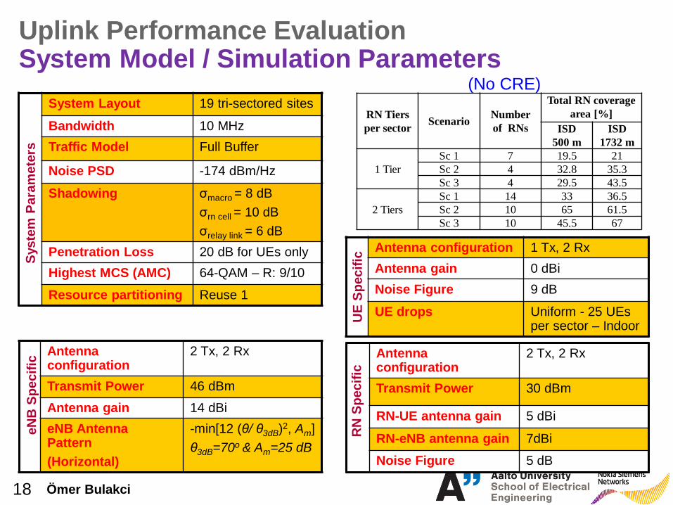
Uplink Performance Evaluation System Model / Simulation Parameters

System Layout 19 tri-sectored sites

Bandwidth 10 MHz Traffic Model Full Buffer

Noise PSD -174 dBm/Hz

Shadowing σmacro = 8 dB σrn cell = 10 dB σrelay link = 6 dB

Penetration Loss 20 dB for UEs only Highest MCS (AMC) 64-QAM – R: 9/10

Resource partitioning Reuse 1

Antenna configuration

2 Tx, 2 Rx

Transmit Power 46 dBm Antenna gain 14 dBi eNB Antenna Pattern (Horizontal)

-min[12 (θ/ θ3dB)2, Am] θ3dB=70o & Am=25 dB

Syst

em P

aram

eter

s eN

B S

peci

fic

Antenna configuration 1 Tx, 2 Rx Antenna gain 0 dBi Noise Figure 9 dB

UE drops Uniform - 25 UEs per sector – Indoor U

E Sp

ecifi

c Antenna configuration

2 Tx, 2 Rx

Transmit Power 30 dBm

RN-UE antenna gain 5 dBi

RN-eNB antenna gain 7dBi

Noise Figure 5 dB

RN

Spe

cific

RN Tiers per sector Scenario Number

of RNs

Total RN coverage area [%]

ISD 500 m

ISD 1732 m

1 Tier Sc 1 7 19.5 21 Sc 2 4 32.8 35.3 Sc 3 4 29.5 43.5

2 Tiers Sc 1 14 33 36.5 Sc 2 10 65 61.5 Sc 3 10 45.5 67

(No CRE)

Ömer Bulakci 19

Reference Scenario: Before Optimization

e2e 50

e2e 40

Access Instantaneous Throughput

100

100 instantaneous

80 instantaneous

20 instantaneous

e2e 10

Achievable Sum Throughput

2/10*all PRB

3/10*all PRB

5/10*all PRB

50

30

20 10

4

6

10

20

50

Resource Sharing

• Power control parameters obtained in macrocell-only deployments are applied on all links.

• No Relay Cell Range Extension. • The number of backhaul subframes is determined according

to the average RN coverage area. Ex: 35.3% 4 Backhaul Subframes

• No Co-scheduling.

20 Ömer Bulakci

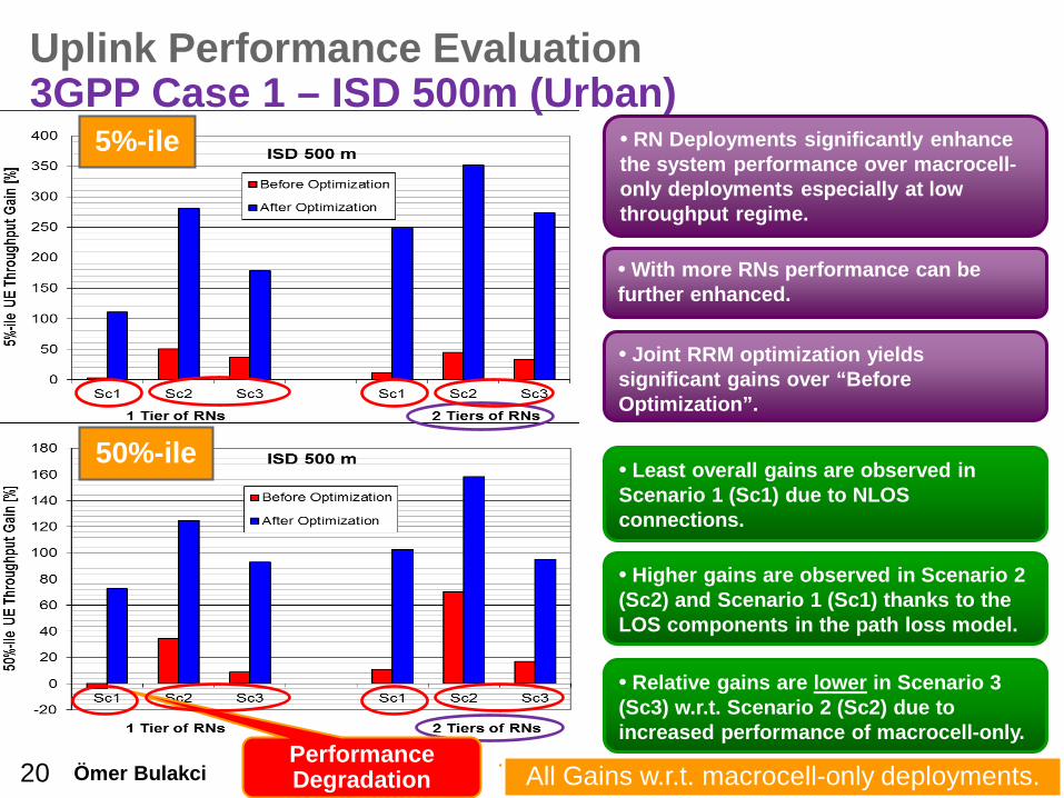
Uplink Performance Evaluation 3GPP Case 1 – ISD 500m (Urban)

5%-ile • RN Deployments significantly enhance the system performance over macrocell-only deployments especially at low throughput regime.

• Least overall gains are observed in Scenario 1 (Sc1) due to NLOS connections.

50%-ile

• With more RNs performance can be further enhanced.

• Joint RRM optimization yields significant gains over “Before Optimization”.

Performance Degradation All Gains w.r.t. macrocell-only deployments.

• Higher gains are observed in Scenario 2 (Sc2) and Scenario 1 (Sc1) thanks to the LOS components in the path loss model.

• Relative gains are lower in Scenario 3 (Sc3) w.r.t. Scenario 2 (Sc2) due to increased performance of macrocell-only.

21 Ömer Bulakci

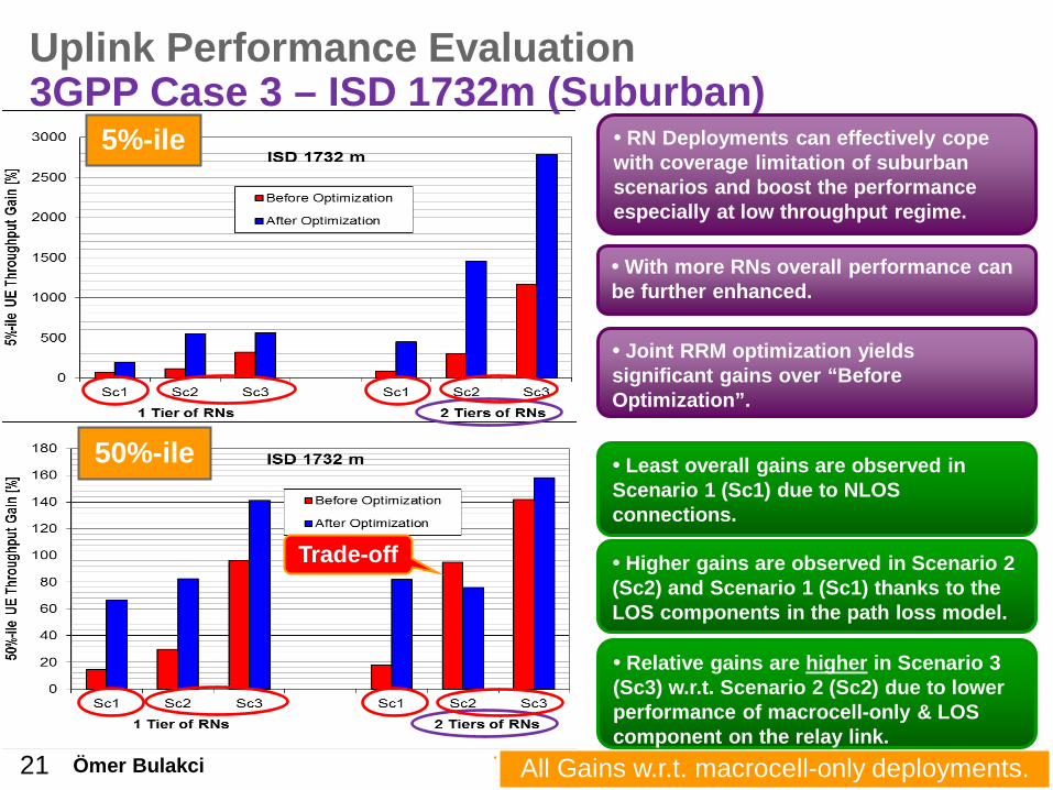
Uplink Performance Evaluation 3GPP Case 3 – ISD 1732m (Suburban)

5%-ile

50%-ile

• RN Deployments can effectively cope with coverage limitation of suburban scenarios and boost the performance especially at low throughput regime.

• Least overall gains are observed in Scenario 1 (Sc1) due to NLOS connections.

• With more RNs overall performance can be further enhanced.

• Joint RRM optimization yields significant gains over “Before Optimization”.

• Higher gains are observed in Scenario 2 (Sc2) and Scenario 1 (Sc1) thanks to the LOS components in the path loss model.

• Relative gains are higher in Scenario 3 (Sc3) w.r.t. Scenario 2 (Sc2) due to lower performance of macrocell-only & LOS component on the relay link.

All Gains w.r.t. macrocell-only deployments.

Trade-off

Content • Goal




• Conclusions

23 Ömer Bulakci

Conclusions

• RN deployments offer significant performance enhancements over macrocell-only deployments

– Especially at low throughput regime – Achieved gains can be significantly different in different

propagation environments ▪ Least gains are observed when all links are NLOS ▪ Higher overall gains are observed when a LOS connection is taken

into account.

• The system performance can be further increased when the

joint optimization of the proposed RRM strategies is applied.

24 Ömer Bulakci

Thank you for your

attention! Q & A

www.nokiasiemensnetworks.com Nokia Siemens Networks St.-Martin-Str. 76 81541 Munich Germany

Ömer Bulakci Ph.D. Candidate [email protected]

25 Ömer Bulakci

BACK-UP

Content • Goal




• Conclusions

27 Ömer Bulakci

OAs are difficult to construct and your required OA may not exist. Hence, we use nearly orthogonal array (NOA):

– Easier to construct. – Can be constructed for any number of experiments – Reduces computational complexity. – Provides similar performance to an OA.

Power Control: Automated Optimization Methodology: Taguchi’s Method

• Let the variable xt where t = 1, 2, 3, 4 designate configuration parameters and γ be any performance measure. The optimization problem is:

)γ(maxarg},,,{4321 ,,,

)opt(4

)opt(3

)opt(2

)opt(1 yxxxx

xxxx=

where is the overall optimization function. )γ(y

• Assume 4 parameters and each can take 3 values. To find the global optimum, we need to test all 34 = 81 combinations.

• Instead, Taguchi’s method uses orthogonal array (OA) that extracts 9 parameter combinations (experiments) from the search space to select nearly-optimal parameter setting.

28 Ömer Bulakci

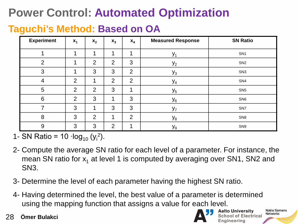
Taguchi’s Method: Based on OA Experiment x1 x2 x3 x4 Measured Response SN Ratio

1 1 1 1 1 y1 SN1

2 1 2 2 3 y2 SN2

3 1 3 3 2 y3 SN3

4 2 1 2 2 y4 SN4

5 2 2 3 1 y5 SN5

6 2 3 1 3 y6 SN6

7 3 1 3 3 y7 SN7

8 3 2 1 2 y8 SN8

9 3 3 2 1 y9 SN9

1- SN Ratio = 10 ∙log10 (yi2).

2- Compute the average SN ratio for each level of a parameter. For instance, the mean SN ratio for x1 at level 1 is computed by averaging over SN1, SN2 and SN3.

3- Determine the level of each parameter having the highest SN ratio.

4- Having determined the level, the best value of a parameter is determined using the mapping function that assigns a value for each level.

Power Control: Automated Optimization

29 Ömer Bulakci

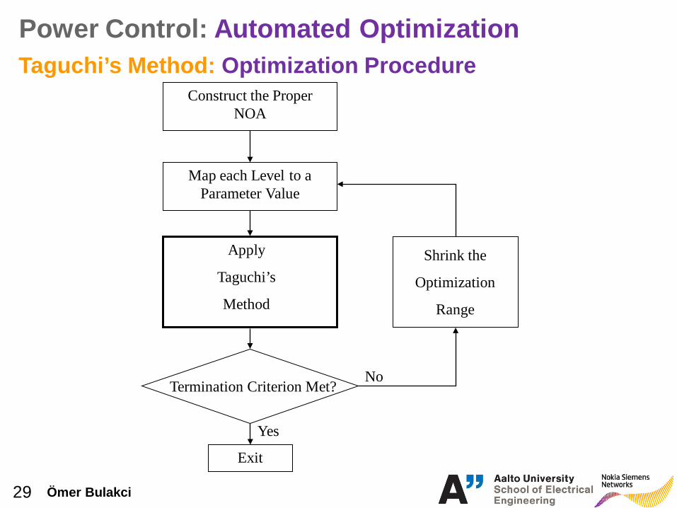
Taguchi’s Method: Optimization Procedure Construct the Proper

NOA

Map each Level to a Parameter Value

Apply

Taguchi’s

Method

Termination Criterion Met?

Exit

Shrink the

Optimization

Range

Yes

No


30 Ömer Bulakci

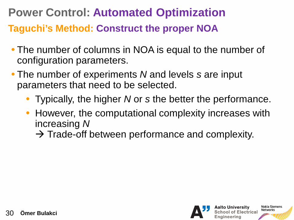
Taguchi’s Method: Construct the proper NOA • The number of columns in NOA is equal to the number of

configuration parameters. • The number of experiments N and levels s are input

parameters that need to be selected. • Typically, the higher N or s the better the performance. • However, the computational complexity increases with

increasing N Trade-off between performance and complexity.


31 Ömer Bulakci


Levels

• In order to perform the experiments, the levels of the NOA should be mapped to testing values.

• In each iteration, the levels of NOA are mapped to new testing values based on the candidate solution found in previous iteration.

• Example: Consider Pmaxrelay-UE [7, 23] dBm and an NOA

having s = 9 levels. In the first iteration,

23 7 15 16.6 18.2 19.8 21.4 13.4 11.8 10.2 8.6 Values

1 2 3 4 5 6 7 8 9

∆ = (23-7) / (9 +1) =1.6

32 Ömer Bulakci


• After applying Taguchi’s method, new values are selected for each parameter.

• Then, the termination criterion ∆ < ε is checked. If not satisfied, the optimization range for each parameter is reduced.

23 7 15 16.6 18.2 19.8 21.4 13.4 11.8 10.2 8.6

Levels

Values

1 2 3 4 5 6 7 8 9 Iteration

1

2

∆’ = ζ*1.6 = 0.8 assuming ζ = 1/2

1 2 3 4 5 6 7 8 9

23 7 16.6

Levels

Values … ... 17.4 15.8

∆’

uplink system performance of lte-advanced relay ... · pdf filelte-advanced relay deployments...

Documents