upper ocean ecosystem dynamics and iron cycling …jkmoore/papers/2004gb002220.pdfupper ocean...

Upper ocean ecosystem dynamics and iron cycling in a global

three-dimensional model

J. Keith MooreEarth System Science, University of California, Irvine, California, USA

Scott C. DoneyDepartment of Marine Chemistry and Geochemistry, Woods Hole Oceanographic Institution, Woods Hole, Massachusetts,USA

Keith LindsayOceanography Section, National Center for Atmospheric Research, Boulder, Colorado, USA

Received 2 January 2004; revised 6 August 2004; accepted 8 September 2004; published 14 December 2004.

[1] A global three-dimensional marine ecosystem model with several key phytoplanktonfunctional groups, multiple limiting nutrients, explicit iron cycling, and a mineral ballast/organic matter parameterization is run within a global ocean circulation model. Thecoupled biogeochemistry/ecosystem/circulation (BEC) model reproduces knownbasin-scale patterns of primary and export production, biogenic silica production,calcification, chlorophyll, macronutrient and dissolved iron concentrations. The modelcaptures observed high nitrate, low chlorophyll (HNLC) conditions in the SouthernOcean, subarctic and equatorial Pacific. Spatial distributions of nitrogen fixation are ingeneral agreement with field data, with total N-fixation of 55 Tg N. Diazotrophs directlyaccount for a small fraction of primary production (0.5%) but indirectly support 10%of primary production and 8% of sinking particulate organic carbon (POC) export.Diatoms disproportionately contribute to export of POC out of surface waters, but CaCO3

from the coccolithophores is the key driver of POC flux to the deep ocean in the model.An iron source from shallow ocean sediments is found critical in preventing ironlimitation in shelf regions, most notably in the Arctic Ocean, but has a relatively localizedimpact. In contrast, global-scale primary production, export production, and nitrogenfixation are all sensitive to variations in atmospheric mineral dust inputs. The residencetime for dissolved iron in the upper ocean is estimated to be a few years to a decade. Mostof the iron utilized by phytoplankton is from subsurface sources supplied by mixing,entrainment, and ocean circulation. However, owing to the short residence time of iron inthe upper ocean, this subsurface iron pool is critically dependent on continualreplenishment from atmospheric dust deposition and, to a lesser extent, lateral transportfrom shelf regions. INDEX TERMS: 0315 Atmospheric Composition and Structure: Biosphere/

atmosphere interactions; 0322 Atmospheric Composition and Structure: Constituent sources and sinks; 1610

Global Change: Atmosphere (0315, 0325); 1615 Global Change: Biogeochemical processes (4805);

KEYWORDS: ecosystem model, nutrient limitation, iron cycle, phytoplankton community

Citation: Moore, J. K., S. C. Doney, and K. Lindsay (2004), Upper ocean ecosystem dynamics and iron cycling in a global

three-dimensional model, Global Biogeochem. Cycles, 18, GB4028, doi:10.1029/2004GB002220.

1. Introduction

[2] Growing appreciation for the key roles played inocean biogeochemistry by phytoplankton functional groupsand trace metal limitation is leading to a new generation ofmore sophisticated, coupled ocean biological, chemical, andphysical models [e.g., Doney, 1999; Doney et al., 2001,2003]. Here we present solutions from one such global

three-dimensional (3-D) model developed by embeddingthe upper ocean ecosystem model of Moore et al. [2002a,2002b] (METa and METb hereinafter, respectively) and anexpanded version of the biogeochemistry module developedas part of the Ocean Carbon Model Intercomparison Project(OCMIP) [Doney et al., 2001, 2003] into the ocean circu-lation component of the Community Climate System Model(CCSM) [Gent et al., 1998; Blackmon et al., 2001]. Ourfocus is on the skill of this coupled biogeochemistry/ecosystem/circulation (BEC) model at representing theobserved basin-scale patterns of biomass, productivity,

GLOBAL BIOGEOCHEMICAL CYCLES, VOL. 18, GB4028, doi:10.1029/2004GB002220, 2004

Copyright 2004 by the American Geophysical Union.0886-6236/04/2004GB002220$12.00

GB4028 1 of 21

community structure, and carbon export as well as thesensitivities of those patterns to changes in external forcing(e.g., atmospheric dust/iron deposition).[3] Shifts in the size-structure and composition of phyto-

plankton communities can strongly influence carbon cy-cling in surface waters and export to the deep ocean. Understrongly nutrient limiting conditions, ecosystems are oftencharacterized by small pico- and nano-sized phytoplankton(more efficient at nutrient uptake than larger phytoplank-ton), strong grazing pressure from microzooplankton, highparticulate organic carbon (POC) recycling, and low verticalcarbon export. Larger phytoplankton, such as diatoms,typically grow quickly under light and nutrient repleteconditions and experience less grazing pressure. Thusdiatoms often dominate episodic blooms and are a majorcontributor to the POC sinking flux from surface waters[Buesseler, 1998]. Coccolithophores are another commoncomponent of blooms, particularly in temperate waters.These phytoplankton form external platelets of calciumcarbonate (CaCO3), a key process affecting carbonatecycling in the oceans that can influence surface waterpCO2 concentrations and air-sea flux [Holligan et al.,1993; Robertson et al., 1994]. The mineral ballast producedby diatoms and coccolithophores also may enhance carbonexport to the deep ocean [Armstrong et al., 2002; Klaas andArcher, 2002]. Diazotrophs, phytoplankton capable of fix-ing N2 gas into more bioavailable nitrogen forms, representa key source of new nitrogen in warm tropical/subtropicalregions [Karl et al., 1997; Capone et al., 1997; Karl et al.,2002; Kustka et al., 2002].[4] Each of these functional groups of phytoplankton is

represented in our ecosystem module (METa; METb).Previously, we validated a version of the model runningin a simple, surface layer physical framework against adiverse set of field observations from nine JGOFS andhistorical time series locations (METa), satellite observa-tions, and global nutrient climatologies (METb). The sim-plified vertical treatment, absence of horizontal advection,and prescribed subsurface nutrient concentrations werelimitations in these simulations, problems alleviated herein the full 3-D implementation. The BEC model includesexplicit iron cycling with external sources to the oceansfrom mineral dust deposition and shallow water sediments.The importance of iron as a key regulator of phytoplanktongrowth and community structure in the oceans is wellestablished, particularly for the high nitrate, low chlorophyll(HNLC) regions [i.e., Martin et al., 1991; Price et al., 1994;de Baar et al., 1995; Coale et al., 1996, Landry, 1997; Boydand Harrison, 1999]. Basin- and global-scale ecosystemmodeling studies have been published during the pastdecade, but most have not included iron as a limitingnutrient [i.e., Sarmiento et al., 1993; Six and Maier-Reimer,1996; Oschlies and Garcon, 1999; Bopp et al., 2001;Palmer and Totterdell, 2001]. Iron cycling has been includedin ecosystem local 1-D simulations [Chai et al., 1996;Loukos et al., 1997; Leonard et al., 1999; Lancelot et al.,2000] and has recently been included in a 3-D ecosystemand circulation model of the equatorial Pacific [Christian etal., 2002] and in two global-scale simulations [Aumont etal., 2003; Gregg et al., 2003].

[5] Significant uncertainties surround the biogeochemicalcycling of iron in the oceans [Johnson et al., 1997; Fung etal., 2000; Johnson et al., 2002]. Johnson et al. [2002]summarize a number of outstanding questions regarding theeffects of speciation, organic ligands, and bioavailability;cellular and detrital iron quotas (i.e., Fe/C ratios); factorsthat control the rates of adsorption to particles (abioticscavenging); and the magnitude of external sources of ironfrom mineral dust deposition/dissolution and ocean sedi-ments. In order to simulate the ocean iron cycle, we havehad to make simplifying assumptions in regard to each ofthese issues. For example, we assume that the dissolved ironpool is completely bioavailable to all phytoplankton withoutregard to speciation or ligand dynamics. These assumptionsare necessary at present to begin to incorporate iron dy-namics into models of ocean biogeochemistry. However, werecognize that many of the key processes are crudelyparameterized and may need to be modified as understand-ing improves.[6] In this work, our emphasis is on annual ecosystem

dynamics, carbon fluxes, and iron biogeochemistry in theupper few hundred meters of the water column at the globalscale. Results are presented from an initial 24-year controlsimulation and several sensitivity experiments. Simulatedupper ocean nutrient concentrations and ecosystem dynam-ics approach a relatively stable, repeating seasonal cycle,after �10 years, and we present results from the final year.The timescale for the deep ocean to reach dynamicalequilibrium is much longer, on the order of several thousandyears, and the interaction of the coupled model on deepocean nutrients will be a focus of future work. Similarly, wewill address seasonal timescale variations in phytoplanktonbiomass and nutrient limitation and detailed comparisonsbetween the model output and field data collected at theJGOFS and historical time series locations elsewhere.

2. Methods

2.1. Ecosystem Implementation

[7] The ecosystem model includes the nutrients nitrate,ammonium, phosphate, dissolved iron (dFe), and silicate(dSi); four phytoplankton functional groups; one class ofzooplankton; dissolved organic matter (DOM); and sinkingparticulate detritus. Coccolithophores (and CaCO3 produc-tion) are included implicitly as a variable fraction of thesmall phytoplankton group. The ecosystem model and itsbehavior in a global surface mixed-layer model are de-scribed in detail in METa and METb. Here we focus ondifferences between this implementation and METa. Forfurther details the reader is referred to METa.[8] The original ecosystem model allows for variable

elemental ratios in all components of the ecosystem, andphytoplankton growth is modeled according to a dynamicgrowth (internal cellular quota) parameterization based onwork by Geider et al. [1998]. The current model assumesfixed C/N/P elemental ratios within phytoplankton groupsand zooplankton, and a fixed Fe/C ratio in zooplankton,significantly reducing the number of advected tracers andcomputational costs. Phytoplankton Fe/C ratios and diatomSi/C ratios are allowed to vary based on ambient nutrient

GB4028 MOORE ET AL.: GLOBAL ECOSYSTEM-BIOGEOCHEMICAL MODEL

2 of 21

GB4028

concentrations. We simulate explicit C, Fe, and chlorophyllpools for each phytoplankton group, and an explicit Si poolfor diatoms. Phytoplankton growth is parameterized accord-ing to a balanced growth model with C/N/P ratios atmodified Redfield values (117/16/1) for diatoms, smallphytoplankton, zooplankton, and sinking detritus based onwork by Anderson and Sarmiento [1994]. The ratio fordiazotrophs is set at 329/45/1 to reflect the high C/P ratiosobserved for Trichodesmium (N/P of 45 [Letelier and Karl,1996]), with the same C/N ratio as the other groups. Allelemental ratios are allowed to vary within DOM.[9] Phytoplankton growth rates are set by modifying the

maximum growth rate for each functional group bywhichever nutrient is most limiting for that group (lowestconcentration relative to uptake half-saturation constants)and light. These limitations are multiplicative so phyto-plankton can be light-nutrient colimited. Chlorophyllcontent and photoadaptation are based on work by Geideret al. [1998] with some modifications (METa). A temper-ature relationship with a q10 factor of 2.0 [Doney et al.,

1996] is used that reduces rates more strongly at lowtemperatures than in METa. This improves seasonal patternsof production and biomass at high latitudes. Ecosystemparameters are listed in Table 1.[10] Model phytoplankton are allowed to adapt to low

available iron levels with some plasticity in their Fe/C ratios[Sunda and Huntsman, 1995, 1997]. Variable Fe/C ratios areimplemented by subtracting iron due to phytoplankton lossterms (e.g., grazing, mortality) at the current Fe/C ratio (Qfe)for each group and then adding new biomass at a growth Fe/C ratio (gQfe) determined by ambient iron concentrationsand the iron uptake half-saturation constant for each group.Optimum Fe/C ratios (Qfeopt) are set for each group and areused when dissolved iron is plentiful relative to the half-saturation constant (dFe > 2 � Kfe). These optimum ratiosare 6 mmol/mol for diatoms and small phytoplankton (METa)and 48 mmol/mol for diazotrophs [Berman-Frank et al.,2001; Kustka et al., 2002, 2004]. As dFe falls below twotimes the half-saturation constant, the growth Fe/C ratiois reduced as gQfe = Qfeopt � dFe/(2 � Kfe). A minimum

Table 1. Key Parameters Used in the Marine Ecosystem Portion of the Coupled BEC Modela

Value Parameter

0.02 fraction of atmospheric iron deposition which dissolves at surface3.0b maximum C-specific growth rates for diatoms and sphyto0.4b maximum C-specific growth rate for diazotrophs0.1 nongrazing mortality term for diatoms and sphyto0.18 nongrazing mortality term for diazotrophs0.009 coefficient in quadratic mortality/aggregation term for diatoms and sphyto2.75b maximum grazing rate on sphyto2.0b maximum grazing rate on diatoms1.2b maximum grazing rate on diazotrophs0.1b linear zooplankton loss term0.46b quadratic zooplankton loss term1.05 coefficient z_grz used in zooplankton grazing rate calculation0.01 inverse timescale of DOM remineralization (100 days)0.5 Ks value for sphyto nitrate uptake2.5 Ks value for diatom nitrate uptake0.005 Ks value for sphyto ammonium uptake0.08 Ks value for diatom ammonium uptake1.0 Ks value for diatom silicate uptake0.0003125 Ks value for sphyto phosphate uptake0.005 Ks value for diatom phosphate uptake0.0075 Ks value for diazotroph phosphate uptake60 Ks value for sphyto iron uptake (pM)160 Ks value for diatom iron uptake (pM)100 Ks value for diazotroph iron uptake (pM)0.25 initial slope of P vs. I curve for diatoms and sphyto (see METa)0.028 initial slope of P vs. I curve for diazotrophs6.0 optimum Fe/C ratio (mmol/mol) for diatoms and sphyto2.5 minimum Fe/C ratio (mmol/mol) for diatoms and sphyto2.5 fixed Fe/C ratio (mmol/mol) for zooplankton48.0 optimum Fe/C ratio (mmol/mol) for diazotrophs14.0 minimum Fe/C ratio (mmol/mol) for diazotrophs0.137 optimum Si/C ratio (mol/mol) for diatoms0.685 maximum Si/C ratio (mol/mol) for diatoms0.0685 minimum Si/C ratio (mol/mol) for diatoms0.137 fixed molar N/C ratio for all phytoplankton and zooplankton0.00855 fixed molar P/C ratio for diatoms, sphyto, and zooplankton0.00304 fixed molar P/C ratio for diazotrophs2.3 maximum Chl/N ratio for (mg Chl/mmolN) for sphyto3.0 maximum Chl/N ratio for (mg Chl/mmolN) for diatoms3.4 maximum Chl/N ratio for (mg Chl/mmolN) for diazotrophs

aSee Moore et al. [2002a] for details. Rates are daily unless noted otherwise. Concentrations are in mM unless noted otherwise.Term ‘‘sphyto’’ denotes small phytoplankton group.

bParameter is scaled by the temperature function.


3 of 21

GB4028

Fe/C ratio of 2.5 mmol/mol is imposed for diatoms and smallphytoplankton, and a minimum of 14 mmol/mol is set fordiazotrophs [Kustka et al., 2002]. Some phytoplanktonspecies are capable of luxury uptake of iron, leading to highFe/C ratios, but luxury uptake is not included. A fixed Fe/Cof 2.5 mmol/mol is set for zooplankton, and if grazed materialhas higher Fe/C ratios, the excess is released as dissolvediron.[11] Diatom Si/C and Si/N ratios increase under iron-

stressed conditions [Takeda, 1998; Hutchins et al., 1998],possibly linked to reduced growth rate through the cell cycle[Martin-Jezequel et al., 2000]. Diatoms also can signifi-cantly reduce their silicification levels under silicon-limitedconditions [Ragueneau et al., 2000]. We allow for bothadaptations in the model with variable Si/C ratios imple-mented in a manner similar to Fe/C. An optimum Si/C ratio(Qsiopt) of 0.137 (mol/mol) is used under nutrient-repleteconditions [Brzezinski, 1985]. When iron uptake is limitedby available dFe and silicate uptake is not, the Si/C ratio fornew biomass is increased up to a maximum value of 0.685,according to gQsi = (Qsiopt � Kfe/dFe) � 5.0) � 0.2. Thisresults in a steep increase in Qsi as iron decreases, reachingthe maximum value when dFe = 0.13 nM. If dissolvedsilicate uptake is significantly limited (dSi < 2.0 � Ksi),then Si/C is not increased under low iron, and the growthSi/C ratio decreases as gQsi = Qsiopt � dSi/(2.0 � Ksi), to aminimum value of 0.0685. Aumont et al. [2003] utilized asomewhat similar parameterization of a variable Si/C ratio,reduced under low Si and increased under low ambient ironconcentrations.[12] Calcification is parameterized in a manner similar to

METa based on the known ecology and global distributionsof coccolithophores [Iglesias-Rodrıquez et al., 2002]. Thebase calcification rate (CaCO3prod), set at 2.4% of the smallphytoplankton primary production rate, is adjusted down-ward under nutrient-limited or low-temperature conditions.We decrease the production of CaCO3 at low temperaturesbased on observations that coccolithophores are rarely foundin cold polar waters. Iglesias-Rodrıguez et al. [2002] foundthat coccolithophore blooms were most often observed attemperatures between 5� and 15�C in satellite data, and wererarely found south of the Antarctic Polar Front (PF) in theSouthern Hemisphere. Summertime temperatures at thepoleward edge of the PF are typically �3�C [Moore et al.,1999]. Thus we progressively reduce the calcification rate astemperatures fall below 5�C as CaCO3prod = CaCO3prod �(TEMP + 2.0)/7.0. We decrease calcification under stronglynutrient-limiting conditions and increase calcification whenthe small phytoplankton group is blooming to try andcapture the community composition typically associatedwith these conditions in the field. When nutrients are scarce,coccolithophores will tend to be outcompeted by smallerpicoplankton that are more efficient at nutrient uptake.Coccolithophores are often a dominant component of non-diatom blooms, particularly in midlatitude temperate regions[Iglesias-Rodrıquez et al., 2002]. Thus, under bloom con-ditions, when the small phytoplankton biomass exceeds3.0 mM carbon, the calcification rate is increased (up to amaximum of 40% of the small phytoplankton primaryproduction) as CaCO3prod = CaCO3prod � (sphytoC/3.0).

Currently, the model does not explicitly include calcificationby other organisms.[13] A single zooplankton pool grazes on all phytoplank-

ton groups, with grazing parameters and the routing amongremineralization and the detrital pools varying depending onthe type of prey being consumed (METa). Thus our singlezooplankton class is able to capture some ecological aspectsof both microzooplankton and macrozooplankton. Field-work suggests that small phytoplankton experience muchstronger grazing pressure from microzooplankton than dothe other phytoplankton groups [i.e., Sherr and Sherr,1988]. Maximum grazing rates are set higher for the smallphytoplankton group, though parameters are such that it ispossible for them to escape grazing control and bloomunder optimal growth conditions. Grazing rates are lowerand more material is routed to sinking detritus whendiatoms are eaten, reflecting generally larger predators(e.g., copepods) and sinking fecal pellet production. Ap-pendix A gives details of the routing of materials fromphytoplankton and zooplankton mortality: between sinkingparticulate organic matter, suspended/dissolved organicmatter, and remineralization to inorganic nutrient pools.

2.2. Remineralization of Detrital Pools

[14] The suspended/dissolved organic matter pool(DOM) in the oceans can be broken into roughly threecomponents: a labile pool that is remineralized quickly on atimescale of hours to days, a semilabile pool that isremineralized on a timescale of months, and a refractorypool that has a lifetime of decades to thousands of yearsand accounts for the large DOM concentrations in the deepocean [i.e., Carlson, 2002]. In the model, the labile DOMpool generated by, for example, phytoplankton excretion isinstantly remineralized to inorganic nutrients. The remain-ing production of DOM is assumed to be semilabile andremineralizes with a lifetime of �100 days. Thus, semi-labile DOM can build up in surface waters over seasonaltimescales and be exported from the euphotic zone. The100-day timescale was chosen to give reasonable seasonalbuildups of DOC given our particular routing of materialsbetween instant remineralization, dissolved organic pools,and sinking particulate detrital pools (see Appendix A). Aswe ignore the refractory portion of the DOM pool, littleDOM is exported to deep waters, and deep ocean concen-trations are negligible. The treatment of DOM in the modelis admittedly crude at present. Future work will seek toimprove the representation of DOM.[15] Sinking detrital organic and mineral ballast pools

instantly sink and remineralize at depth in the same gridpoint where they originate. Fast-sinking particles could notadvect far from their source location due to slow currentspeeds at depth and our coarse resolution. As the sinkingparticulate pool is now implicit, it is not grazed by zoo-plankton as in METa. Remineralization at depth is prescribedbased on the mineral ballast model of Armstrong et al.[2002]. Organic matter entering the sinking detrital pool isdivided into a ‘‘free’’ organic fraction (easily remineralized)and a mineral ballast associated fraction, which remineral-izes deeper in the water column with the correspondingmineral dissolution. A portion of each mineral ballast (and


4 of 21

GB4028

its associated POM) is assumed to be fast sinking andresistant to degradation and thus to sink to the bottom ofthe ocean before remineralization.[16] Mineral ballast consists of dust from the atmosphere,

CaCO3 from the coccolithophores, and biogenic silica (bSi)from the diatoms. Three parameters are set for each ballasttype: (1) the mass ratio of associated organic carbon/mineralballast; (2) the ballast dissolution length scale of the ‘‘soft’’ballast fraction; and (3) the ‘‘hard’’ ballast fraction thatmostly dissolves in the bottom model cell (assigned a verylong, but not infinite, remineralization length scale of40,000 m in our simulations). In addition, there is aremineralization length scale for the ‘‘free’’ POM. Theorganic carbon/mineral ballast mass ratios are based largelyon the sediment trap analysis of Klaas and Archer [2002].The remineralization length scales for ‘‘free’’ POM and bSiincrease with decreasing water temperature using thetemperature rate function from the ecosystem model. Thedissolution of bSi is known to be strongly influenced bytemperature, and significantly steeper temperature functionshave been used [e.g., Gnanadesikan, 1999]. The mineralballast model parameter values are presented in Table 2. Thesinking detrital pool has variable dust/bSi/CaCO3/C/Feratios with C/N/P fixed at Redfield values. As describedin Appendix S, 10% of scavenged iron is added to thissinking pool. Dissolved iron is released as portions of thesinking dust pool dissolve/remineralize at depth, assumingan iron content of 3.5% by weight. The current simulationsare too short to examine how the mineral ballast modelinfluences deep ocean nutrient distributions over longtimescales.

2.3. Iron Cycling

[17] We make a number of simplifying assumptions toincorporate iron dynamics. All dissolved iron is assumedavailable for uptake by phytoplankton with no regard forspeciation or ligand interactions. In METa, nutrient concen-trations below the surface mixed layer were held constant.Iron scavenging rates were set high where dissolved ironexceeded 0.6 nM, the high dust deposition regions, and at alow background rate elsewhere. Initial experiments with the3-D model showed that this background rate was much too

low, leading to a rapid buildup of dissolved iron in the upperfew hundred meters of the water column in many regions. Itis this scavenging onto particles and subsequent removalthat keeps subsurface nutrient pools deficient in iron relativeto macronutrients. Thus, scavenging rates for dissolved ironhave been increased significantly over those in METa andare parameterized as a more complicated function of sinkingparticle flux (dust and particulate organic carbon (POC)),standing particle concentration (POC pools), and the ambi-ent iron concentration (see Appendix A).[18] The model is forced with a simulated dust climatol-

ogy, over the period 1979–2000, validated against mea-surement sites around the globe [Luo et al., 2003]. Thefraction of iron that dissolves upon surface dust depositionis uncertain and likely varies depending on atmosphericprocessing and deposition pathway (wet versus dry)[Jickells and Spokes, 2001], but little information is availableat present to develop a global parameterization [Fung et al.,2000]. Dust iron content and surface solubility are thereforeset at fixed values of 3.5% iron by weight and 2.0%,respectively. In prior modeling efforts, iron releaseis assumed to occur only in surface waters [Archer andJohnson, 2000; Christian et al., 2002; Moore et al., 2002a,2002b; Aumont et al., 2003]. However, further dissolution/iron release may happen deeper in the water column as theresult of slow dissolution from fast sinking dust particles/aggregates or consumption of dust particles by grazers,where a substantial release of iron is likely due to low pHlevels in the gut [Barbeau et al., 1996]. To account forthese processes, an additional 3% of the dust is prescribedto dissolve within the water column with a remineralizationlength scale of 600 m. We make this somewhat arbitraryassumption based on the idea that the likelihood of a dustparticle passing through an animal gut is greatest in theupper water column and decreases at greater depths, fol-lowing the general vertical distribution of grazer biomass.The remaining dust/iron remineralizes with a long lengthscale as described above for ballast materials (40,000 m).Sinking dust particles also act to scavenge dissolved ironand remove it to the sediments (Appendix A). In the upperocean, the scavenging due to dust is small in most regionscompared with that due to biogenic particles. However, inthe deep ocean, sinking dust particles account for a signif-icant fraction of total scavenging in the model.[19] Sediments are an important source of dissolved iron

to oceanic waters [Johnson et al., 1999; de Baar and deJong, 2001], but little quantitative information is availablefor parameterizations of this process. In METa, we set thefixed subsurface iron concentrations higher in shallowregions to account for this source. Johnson et al. [1999]estimated a diffusive flux out of the sediments in the coastalupwelling system off California (a high productivity region)at 5 mmol Fe/m2/day, noting that the iron flux from sedimentresuspension was likely even larger. As a first, admittedlycrude attempt, we include a uniform sediment iron source of2 mmol Fe/m2/day for areas where depth is less than 1100 m.Inputs are likely too low in shallow, highly productiveregions and too high in deeper areas underlying lowerproductivity waters. However, even this simple parameter-ization notably improves the model results in several

Table 2. Parameter Values Used in the Mineral Ballast Model of

Particulate Remineralization Through the Water Columna

Length, m %Hard OCRatio

Soft POM 70–643b – –(C, N, P, Fe,)

Biogenic Si 70–643b 60 0.035CaCO3 600 60 0.07Mineral dust 600 95 0.07

aValues based on Armstrong et al. [2002] and Klaas and Archer [2002].Length is the lengthscale of remineralization for the soft portion ofballast and associated POM, %Hard is the fraction assumed resistant toremineralization, and OCRatio is the assumed bound organic carbon/mineral ballast ratio by weight. A portion of the POM is bound to eachmineral ballast and has the same remineralization profile as the ballast. Thehard portion of each ballast and the associated POM remineralize with along length scale of 40,000 m (see text for details).

bParameter is scaled by our temperature function, range given for 30� to�2�C.


5 of 21

GB4028

regions. In the results section, we discuss the sensitivity tomodifications of the sedimentary iron source.

2.4. Ocean Circulation Model and AtmosphericForcings

[20] The ocean circulation model is a preliminary versionof the CCSM 2.0 Parallel Ocean Program (POP) code basedon the Los Alamos National Laboratory POP V1.4.3. Themodel has 100 � 116 horizontal grid points with a resolu-tion of 3.6� longitude and 0.9�–2� latitude (higher near theequator) and a Northern Hemisphere pole rotated intoGreenland. There are 25 vertical levels, and the surfacelayer is 12 m thick, with five levels in the upper 111 m. Themodel employs the Gent-McWilliams isopycnal mixingparameterization [Gent and McWilliams, 1990] and theKPP upper ocean model [Large et al., 1994]. Daily atmo-spheric forcings are from a 4-year (1985–1989) repeat cycleof NCEP/NCAR reanalysis data [Large et al., 1997; Doneyet al., 1998].

2.5. Initial Conditions and Biogeochemical Spin-Up

[21] Zooplankton, DOM, and phytoplankton pools areinitialized uniformly at low values. Initial distributions ofphosphate, nitrate, and silicate are taken from annual meanvalues in the World Ocean Atlas 1998 database [Conkrightet al., 1998]. Initial values for alkalinity, dissolved oxygen,and dissolved inorganic carbon are from the OCMIP bioticmodel simulations conducted at NCAR [Doney et al., 2001,2003]. Following a physical spin-up to approximatelysteady state, the biogeochemical/ecosystem model controland sensitivity runs are integrated for 24 years, with resultspresented here from the final year of the simulation. A third-order upwind advection scheme is employed for tracer

transport. Small, negative values in surface concentrationsarising from advection errors are treated as zero in thebiological code and for plotting here.[22] The lack of a global dissolved iron database is a

critical problem facing ocean biogeochemical modelingtoday [Johnson et al., 2002]. Initially, dissolved iron wasset with summer surface values from our mixed layer model(METb) and assigned regional to basin-scale vertical pro-files based on sparse published literature values. Thesedepth profiles increased linearly from the surface concen-tration to 0.6 nM at depth (typically between 400 and600 m). The deep ocean was set to a uniform initial valueof 0.6 nM except for the high-latitude Southern Ocean,where 0.4 nM is applied with a linear transition region from40�S–50�S. In early simulations, mean iron concentrationin the upper 111 m of the water column increased rapidly,roughly doubling during the first decade. This increase wasdue to lateral spreading of the sedimentary iron source,adjustment to the new scavenging parameterization, anddrift in subsurface iron concentrations (in many areas theslope with depth was not linear to 400–600 m). Here weuse the iron field from year 12 of a preliminary run as ourinitial dissolved iron distribution. The drift in mean con-centrations in the upper 111 m over the last 4-year forcingcycle was <1% for all nutrients.

3. Results

[23] Similar to our previous findings (METb), the eco-system model captures to a large degree the observed, large-scale spatial patterns and seasonal cycles in key surfaceocean metrics, including nutrient and dissolved iron con-centrations (Figures 1 and 2; WOA98, Table 1 of METb,

Figure 1. Surface nitrate and phosphate concentrations (summer season in each hemisphere) arecompared with climatological concentrations from the World Ocean Atlas 1998.


6 of 21

GB4028

and work by Johnson et al. [1997] and de Baar and de Jong[2001]), surface chlorophyll (Figure 3; SeaWiFS),and primary production (Figure 4; SeaWiFS with VGPMalgorithm). Here we highlight key features, differenceswith the mixed layer model results, and remaining deficien-

cies. The most significant result is that the inclusion ofexplicit iron dynamics allows the model to reproduce theHNLC conditions in the Southern Ocean and equatorial andsubarctic Pacific Ocean (METa, METb). However, theequatorial Pacific HNLC region is larger in spatial extent

Figure 2. Surface silicate concentrations (summer season in each hemisphere) are compared withclimatological concentrations from the World Ocean Atlas 1998. Also shown are the summer and winterseason surface dissolved iron concentrations from the model.

Figure 3. Model surface chlorophyll are compared with SeaWiFS satellite estimates for the months of(a, c) June and (b, d) December.


7 of 21

GB4028

in the model than in observations, most likely due toexcessive upwelling, a common problem with coarse reso-lution models (see discussion in section 5).[24] Surface phosphate concentrations are strongly

depleted in the North Atlantic gyre due to substantialnitrogen fixation rates early in the simulation. Elsewhere,light and/or iron limitation of nitrogen fixation prevents suchstrong phosphate depletion. Phosphate concentrations arehigher than observations over much of the western Pacificbasin where the model has essentially zero surface nitrate,suggesting too little nitrogen fixation and phosphate draw-down. Silicate patterns at basin scale are in broad agreementwith the observations but with generally lower surfacevalues (Figure 2). The model does not currently includepossibly important silicon sources from dust deposition andriverine runoff. Note the strong Amazon silicate plume in theWOA98 data (Figure 2). Macronutrient concentrations arelower than observations over parts of the subarctic NorthPacific but are never fully depleted over the annual cycle.[25] Model iron concentrations exhibit significant sea-

sonal variability at high latitudes and in the Arabian Sea(Figure 2). In the Southern Ocean, wintertime iron concen-trations range from 250 to 350 pM, with a summerdrawdown below 150 pM in many areas, in good agreementwith recent observations in the SW Pacific [Measuresand Vink, 2001]. Subarctic North Pacific wintertime ironconcentrations are somewhat higher between 300 and350 pM, reflecting higher atmospheric iron inputs. Ironconcentrations are perpetually very low in the equatorialPacific. High iron concentrations associated with the

mineral dust plumes from North Africa and the ArabianPeninsula [Mahowald et al., 2003; Zender et al., 2003]peak during summer season, with large areas exceeding1.0 nM. Relatively high dissolved iron concentrations alsoare seen over much of the Arctic Ocean due to thesedimentary iron source and the large shelf areas in thisregion.[26] Similar to satellite estimates and METb, model

surface chlorophyll concentrations exhibit lowest levels inmid-ocean gyres and at high latitudes during winter, mod-erate levels (0.2–0.5 mg/m3) in the HNLC regions, andhigh levels in the Arctic and North Atlantic in June and inparts of the Southern Ocean in December. Note thatchlorophyll concentrations remain well below 1.0 mg/m3

over most of the Southern Ocean despite high concentra-tions of the macronutrients (compare with Figures 1 and 2).In general, the model underpredicts chlorophyll concentra-tions in the eastern boundary current upwelling regions andin coastal waters. The physical processes associated withcoastal upwelling are only weakly captured in our coarseresolution ocean model.[27] Compared with a satellite-based estimate from

the Vertically Generalized Production Model (VGPM)[Behrenfeld and Falkowski, 1997], model annual meanprimary production (Figure 4) is higher in the tropicalupwelling zones and over much of the Southern Oceanand lower in the subpolar North Atlantic and North Pacific.Schlitzer [2000] suggests that VGPM underestimatesproduction in the Southern Ocean and overestimates pro-duction in the North Atlantic based on an inverse modeling

Figure 4. Model simulated annual primary production is compared with a satellite-based productivityestimate using the Vertically Generalized Production Model of Behrenfeld and Falkowski [1997] (seeMoore et al. [2002b] for details of this production estimate).


8 of 21

GB4028

approach. Buesseler et al. [2003] also notes that the VGPMunderpredicts Southern Ocean productivity relative to fieldobservations along 170�W. The productivity patterns pre-sented here are similar to our previous results (METb),except for the equatorial upwelling regions where produc-tion is significantly higher.

4. Export Fluxes

[28] The spatial patterns of annual sinking export ofparticulate organic carbon (POC), biogenic silica, andcalcium carbonate at the base of the euphotic zone (111 mdepth) (Figure 5) are similar to those from the mixed layerversion (compare with Figures 7 and 12 of METb). Thetotal POC flux, however, is lower at 5.8 GtC at 111 m depthcompared with 7.9 GtC at the base of the mixed layer inMETb. The coarse resolution GCM is not able to sustainsuch high export fluxes and is on the low end of model andobservational estimates [Oschlies, 2001]. Note, however,that export estimates are sensitive to the depth chosen todefine the bottom of the net production or euphotic zone asthere is a substantial vertical gradient in POC flux withdepth (sinking flux is 6.6 GtC at 49 m [see also Doney etal., 2003]). The POC export patterns are driven largely by

diatoms (see bSi export) and coccolithophores (see CaCO3

export). Annual export ratios (sinking/PP) range from 0.04to 08 in the mid-ocean gyres to 0.2–0.38 in mid- to high-latitude bloom regions. Antia et al. [2001] estimated annualexport ratios (at 125 m) ranging from 0.08 to 0.38 from alarge number of sediment trap studies throughout the NorthAtlantic. Of the dissolved organic carbon (DOC) productionof 12.1 GtC, 0.31 GtC is exported from the euphotic zoneand remineralized below 111 m (0.49 GtC below 49 m),mainly at high latitudes where there is deep convectivemixing in winter.[29] Most of the model sinking POC pool (global average

of 93.4%, at 111 m) is in the easily degraded ‘‘free’’ POCfraction, with remineralization length scales varying be-tween 70 and 643 m (dependent on temperature). Theremaining fraction (6.6%) associated with mineral ballast[Armstrong et al., 2002] has much longer remineralizationlength scales (see Table 2), strongly influencing the POCflux to the deep ocean. The amount of POC associated witheach ballast type is a function of the model parameteriza-tion, the atmospheric dust deposition, and the CaCO3 andbSi production from the ecosystem model. At 111 m depth,57.6% of the bound POC is associated with CaCO3,34.2% with bSi, and 8.2% with sinking dust particles.

Figure 5. Annual sinking export at 111 m depth of particulate organic carbon, biogenic silica, andcalcium carbonate are depicted.


9 of 21

GB4028

This is partially a function of the prescribed higher organicC/ballast ratio for CaCO3 (Table 2). Thus CaCO3 fluxdominates transport of organic carbon to the deep oceanin the model. A reasonable range for the calcification/photosynthesis ratio for coccolithophores is 0.2–1.0[Robertson et al., 1994; Balch et al., 1996]. This rangeimplies coccolithophores in the model account for �1–4%of primary production. In contrast, diatoms contribute 46%of sinking POC export out of the euphotic zone (including‘‘free’’ and ballast associated fractions) and 32% of totalprimary production (compared with 24% in METb).Aumont et al. [2003] found that diatoms and their meso-zooplankton grazers accounted for 55% of sinking exportand 20% of production. Nelson et al. [1995] estimated amaximum diatom productivity contribution of 43%, includ-ing productive coastal waters.[30] As in METb, the spatial patterns of CaCO3 produc-

tion and export are in generally good agreement with theglobal sediment trap synthesis of Milliman [1993] andsatellite-based estimates of coccolithophore bloom distribu-tions [Brown and Yoder, 1994; Brown and Podesta, 1997;Iglesias-Rodrıguez et al., 2002]. Highest calcification ratesand CaCO3 export are seen over the Patagonian shelf and insome other midlatitude Southern Ocean regions, in thecoastal and equatorial upwelling zones, in the ArabianSea, and in parts of the North Atlantic (Figure 5). Theglobally integrated calcification is 0.53 GtC, with 0.25 GtCsinking across 1100 m. Milliman et al. [1999] estimateglobal calcification as 0.7 GtC with the flux to the deepocean (>1000 m) of �0.3 GtC. Model estimates of deepocean sinking fluxes at 1100 m for POC and bSi are 0.59GtC and 41 Tmol Si, respectively.[31] The model rain ratio (sinking CaCO3/sinking POC)

at 111 m integrated globally is 0.065. Yamanaka and Tajika[1996] estimate the global rain ratio to be between 0.08 and0.1. Sarmiento et al. [2002] recently argue for a value of�0.06, with peak values near the equator (>0.08), lowervalues in the gyres, and minimum values at high latitudes.Their data-model synthesis had a very low rain ratio (0.023)in the North Atlantic, surprising as this region is known forfrequent coccolithophore blooms. Our simulated rain ratiosover most of the mid- to high-latitude North Atlantic are0.07–0.12, with a small area exceeding 0.25. We simulaterelatively high rain ratios in the gyres (�0.09–0.15) andgenerally low values at high southern latitudes (<0.05).These patterns in the rain ratio are quite different than thespatial patterns of absolute CaCO3 production. Despiteelevated CaCO3 export, the rain ratio in coastal and equa-torial upwelling zones is typically low due to high levels ofPOC export (Figure 5).[32] Global biogenic silica production in the model is 189

Tmol Si, with about a third (63 Tmol Si) exported across111 m. The biogenic Si export ratio varies as a function oftemperature and the fraction of diatom mortality due tograzing and nongrazing pathways (see section 2 and Ap-pendix A). Nelson et al. [1995] estimate a global bSiproduction of 200–280 Tmol Si/yr and a sinking exportof 100–140 Tmol Si based on an assumed export ratio of50%, and Gnanadesikan [1999] computes bSi export at89 Tmol, arguing that the total is likely �100 Tmol. Nelson

et al. [1995] note that at least 50% of bSi dissolves in theupper 100 m of the ocean, with an average dissolution of58% (export ratio of 0.42) in their observational data sets.Our lower export ratio includes Si released through non-grazing mortality meant to account for viral losses andleakage from cells. In the radiolabeled Si studies cited byNelson et al. [1995], Si that is taken up but then leaks fromthe cell during the incubation would not be accounted for,possibly reconciling our lower export ratios. Nelson et al.[1995] also include coastal diatom production, which isonly weakly captured in our GCM.[33] Regionally, model areal annual bSi production rates

qualitatively agree with field estimates. Compared withNelson et al. [1995], model rates are: generally below 0.1versus 0.2 mol/m2/yr for the mid-ocean gyres, wherediatom production is likely driven by nutrient input fromeddies and other mesoscale processes not included inthe physical model; 1–2 versus above 8 mol/m2/yr forunderresolved coastal upwelling areas; 0.4–2.0 versus2.2 mol/m2/yr for the subarctic Pacific; and 0.3–2.0 versus0.4–1.0 mol/m2/yr for the Southern Ocean. Model bSiproduction rates are higher in the southwest Atlantic sectorand the southwest Pacific sector of the Southern Ocean,exceeding 2.0 molSi/m2/yr. Recent observations during theU.S. JGOFS Southern Ocean study along 170�W foundannual production rates of 1.9–3.0 molSi/m2/yr [Nelson etal., 2001]. Ragueneau et al. [2000] summarize availablesediment trap data of sinking bSi (mainly from >1000 m)and note a strong latitudinal dependence with low-latitudebSi fluxes typically <0.2 molSi/m2/yr and fluxes in themid-ocean gyres <0.03 molSi/m2/yr. Higher fluxes at theselatitudes are seen in coastal upwelling zones and in theequatorial Pacific. Highest sinking fluxes were in theSouthern Ocean and the North Pacific, ranging from0.4 to 0.9 molSi/m2/yr [Ragueneau et al., 2000] (comparewith Figure 5).

4.1. Nitrogen Fixation and Nutrient LimitationPatterns

[34] The spatial pattern of nitrogen fixation in the modelis similar to METb (Figure 6), but the total of 55.5 TgN/yris lower (62.4 TgN in METb) and well below recentobservational (80 TgN [Capone et al., 1997]) and geochem-ical estimates (>100 TgN [Gruber and Sarmiento, 1997;Deutsch et al., 2001; Karl et al., 2002]). Such high rates arenot sustainable in our coarse resolution GCM; possibly thisis because eddies, storms, and other mesoscale processesthat are important sources of new nutrients in tropical andsubtropical regions are not represented. Also, our sinkingexport of biogenic material is forced to be a constant molarN/P ratio of 16. However, the N/P ratio of sinking materialat HOT is consistently �16 during times of N fixation[Christian et al., 1997; Karl et al., 2002], and observationsin the North Atlantic at BATS show elevated PON/POP andDON/DOP ratios [Ammerman et al., 2003]. Thus, in ourmodel, increasing N fixation tends to deplete phosphatebelow observed concentrations, causing strong P limitationof the diazotrophs, mainly in the North Atlantic.[35] As in METb, elevated nitrogen fixation is simulated

along the northern coasts of South America and Australia,


10 of 21

GB4028

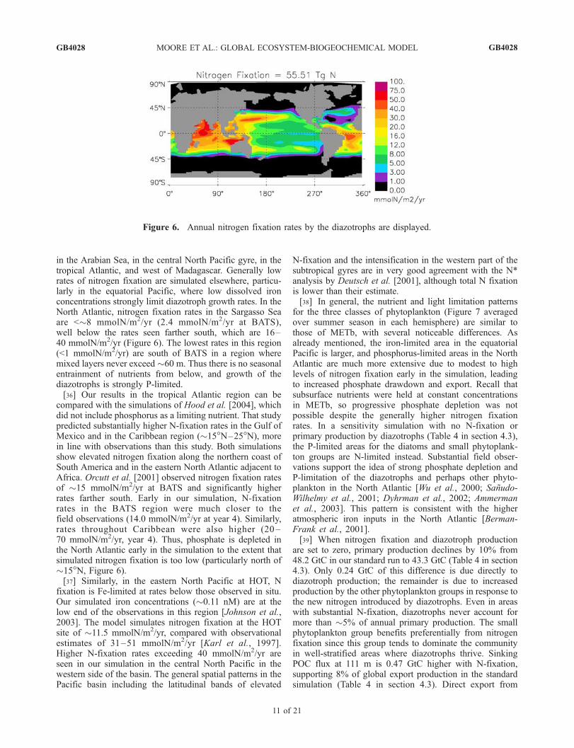
in the Arabian Sea, in the central North Pacific gyre, in thetropical Atlantic, and west of Madagascar. Generally lowrates of nitrogen fixation are simulated elsewhere, particu-larly in the equatorial Pacific, where low dissolved ironconcentrations strongly limit diazotroph growth rates. In theNorth Atlantic, nitrogen fixation rates in the Sargasso Seaare <�8 mmolN/m2/yr (2.4 mmolN/m2/yr at BATS),well below the rates seen farther south, which are 16–40 mmolN/m2/yr (Figure 6). The lowest rates in this region(<1 mmolN/m2/yr) are south of BATS in a region wheremixed layers never exceed �60 m. Thus there is no seasonalentrainment of nutrients from below, and growth of thediazotrophs is strongly P-limited.[36] Our results in the tropical Atlantic region can be

compared with the simulations of Hood et al. [2004], whichdid not include phosphorus as a limiting nutrient. That studypredicted substantially higher N-fixation rates in the Gulf ofMexico and in the Caribbean region (�15�N–25�N), morein line with observations than this study. Both simulationsshow elevated nitrogen fixation along the northern coast ofSouth America and in the eastern North Atlantic adjacent toAfrica. Orcutt et al. [2001] observed nitrogen fixation ratesof �15 mmolN/m2/yr at BATS and significantly higherrates farther south. Early in our simulation, N-fixationrates in the BATS region were much closer to thefield observations (14.0 mmolN/m2/yr at year 4). Similarly,rates throughout Caribbean were also higher (20 –70 mmolN/m2/yr, year 4). Thus, phosphate is depleted inthe North Atlantic early in the simulation to the extent thatsimulated nitrogen fixation is too low (particularly north of�15�N, Figure 6).[37] Similarly, in the eastern North Pacific at HOT, N

fixation is Fe-limited at rates below those observed in situ.Our simulated iron concentrations (�0.11 nM) are at thelow end of the observations in this region [Johnson et al.,2003]. The model simulates nitrogen fixation at the HOTsite of �11.5 mmolN/m2/yr, compared with observationalestimates of 31–51 mmolN/m2/yr [Karl et al., 1997].Higher N-fixation rates exceeding 40 mmolN/m2/yr areseen in our simulation in the central North Pacific in thewestern side of the basin. The general spatial patterns in thePacific basin including the latitudinal bands of elevated

N-fixation and the intensification in the western part of thesubtropical gyres are in very good agreement with the N*analysis by Deutsch et al. [2001], although total N fixationis lower than their estimate.[38] In general, the nutrient and light limitation patterns

for the three classes of phytoplankton (Figure 7 averagedover summer season in each hemisphere) are similar tothose of METb, with several noticeable differences. Asalready mentioned, the iron-limited area in the equatorialPacific is larger, and phosphorus-limited areas in the NorthAtlantic are much more extensive due to modest to highlevels of nitrogen fixation early in the simulation, leadingto increased phosphate drawdown and export. Recall thatsubsurface nutrients were held at constant concentrationsin METb, so progressive phosphate depletion was notpossible despite the generally higher nitrogen fixationrates. In a sensitivity simulation with no N-fixation orprimary production by diazotrophs (Table 4 in section 4.3),the P-limited areas for the diatoms and small phytoplank-ton groups are N-limited instead. Substantial field obser-vations support the idea of strong phosphate depletion andP-limitation of the diazotrophs and perhaps other phyto-plankton in the North Atlantic [Wu et al., 2000; Sanudo-Wilhelmy et al., 2001; Dyhrman et al., 2002; Ammermanet al., 2003]. This pattern is consistent with the higheratmospheric iron inputs in the North Atlantic [Berman-Frank et al., 2001].[39] When nitrogen fixation and diazotroph production

are set to zero, primary production declines by 10% from48.2 GtC in our standard run to 43.3 GtC (Table 4 in section4.3). Only 0.24 GtC of this difference is due directly todiazotroph production; the remainder is due to increasedproduction by the other phytoplankton groups in response tothe new nitrogen introduced by diazotrophs. Even in areaswith substantial N-fixation, diazotrophs never account formore than �5% of annual primary production. The smallphytoplankton group benefits preferentially from nitrogenfixation since this group tends to dominate the communityin well-stratified areas where diazotrophs thrive. SinkingPOC flux at 111 m is 0.47 GtC higher with N-fixation,supporting 8% of global export production in the standardsimulation (Table 4 in section 4.3). Direct export from

Figure 6. Annual nitrogen fixation rates by the diazotrophs are displayed.


11 of 21

GB4028

diazotrophs is negligible in the current model formulation(Appendix A), and this export is mainly due to the diatomsand small phytoplankton. Without N-fixation, there are noareas where phytoplankton growth is P-limited duringsummer months (compare with Figure 7). Recall that oursimulations are on the low end of observational and geo-chemical estimates of global nitrogen fixation rates. Thusour results should be viewed as minimal estimates of theglobal impact of nitrogen fixation.[40] Model phytoplankton can be limited by light,

nutrients, and temperature or be ‘‘replete.’’ Temperaturelimitation applies only to the diazotrophs, whose growthrates are drastically reduced at temperatures below 15�C inour model. Light and nutrient limitation are multiplicative(METa), and in Figure 7 we plot the most limiting growthfactor in surface waters during summer months. Phyto-plankton are termed nutrient and light replete if they are

growing at >90% of their maximum temperature-dependentrate. These conditions tend to occur when strong grazingpressure prevents blooms that would otherwise depletenutrients. This 90% cutoff is an arbitrary definition; usinga cutoff of 85% increases the replete area for the smallphytoplankton group (mainly in HNLC regions), but haslittle impact on the diatoms. The diatoms and small phyto-plankton are light-limited mainly in high-latitudes areaswith heavy sea ice cover and some lower latitude areasdue to self-shading within blooms. Owing to their substan-tially lower initial slope of the production versus irradiancecurve, diazotrophs are light-limited over portions of thetropical/subtropical oceans. Most tropical/subtropical areasare iron-limited for the diazotrophs (70% of the areas wheretemperature is not restricting their growth). The results areconsistent with the suggestion by Berman-Frank et al.[2001] that for Trichodesmium spp., iron is the limiting

Figure 7. Factor most limiting growth rates is plotted for each phytoplankton group during summermonths in each hemisphere.


12 of 21

GB4028

nutrient throughout most of the world ocean. However, ourresults also point to a significant role for the light regime incontrolling nitrogen fixation [Hansell and Feely, 2000;Moore et al., 2002b; Hood et al., 2004). We can definenutrient-light colimitation as reductions of at least 10% dueto the most limiting nutrient, and by at least 10% due tolight (phytoplankton growing at �80% of their maximumrates). By this definition, 20.3% of the ocean is iron-lightcolimited, and 4.8% if phosphorus-light colimited for thediazotrophs. Smaller areas are iron-light colimited for thesmall phytoplankton (10.0%) and for the diatoms (4.3%).This definition of colimitation is also arbitrary; if 15%reductions in growth are required, the areas colimiteddecrease substantially.[41] The major HNLC regions in the subarctic North

Pacific, equatorial Pacific, and Southern Ocean are mainlyiron-limited for both diatoms and small phytoplankton.Portions of the Southern Ocean are nutrient-replete(essentially ‘‘grazer-limited’’) for the small phytoplanktonwhen averaged over summer months, but by late summerthese areas also tend to be iron-limited. Small phytoplank-ton are iron-limited over much of the high-latitude NorthAtlantic, a pattern seen in METb and Fung et al. [2000].Diatoms are Si-limited in the North Atlantic and largeportions of the equatorial Pacific. Field observations indi-cate that Si-limitation terminated the spring diatom bloomduring the NABE study [Sieracki et al., 1993]. Most of theSi-limited areas in the Pacific are within our expandedHNLC region and may be partly an artifact of excessiveupwelling. In the simulation intense diatom blooms, largerthan observed in situ, occur on the equator, depleting Sirelative to other macronutrients in the upwelling water. Sigrowth regulation in this region has been a topic ofsome debate [Dugdale and Wilkerson, 1998; Dunne etal., 1999; Leynaert et al., 2001]. Aumont et al. [2003]found no Si-limitation in this region but had similarpatterns of Si-limitation in the North Atlantic and moreSi limitation in the subantarctic Southern Ocean. Globally,the diatoms and small phytoplankton are iron-limited over26% and 37% of the world ocean, respectively. Aumont etal. [2003] predict that diatom are iron-limited over 40%of the ocean, with much of the difference due to reducedSi-limitation in their simulation. Less of the ocean is iron-limited than in our previous work with the simple physicalmodel (39% for diatoms and 50% for small phytoplankton,METB). Substantial tropical regions in the Indian andAtlantic oceans were iron-limited in that simulation,probably because our fixed subsurface iron concentrationswere set too low. The iron-limited areas in the subarcticNorth Pacific and in the Southern Ocean were alsosomewhat larger in METB.

4.2. Iron Cycling

[42] Annual dissolved iron uptake by the phytoplanktonis 20.7 � 109 mol Fe, similar to the 18 � 109 mol Fe/yrsimulated by Aumont et al. [2003]. This is surprising giventhe differences in phytoplankton community compositionand Fe/C ratios in the two models. Diazotrophs accountfor 4.3% of iron uptake, but only 0.5% of primaryproduction, due to their elevated demand for iron (high

Fe/C ratios). The global mean Fe/C ratio in our simulationwas 5.1 mmol/mol, with considerable regional variations.This is quite similar to the mean value of 5 mmol/molsuggested by Johnson et al. [1997] and the value of5.1 mmol/mol simulated by Aumont et al. [2003]. MeanFe/C in sinking export at 111 m was 5.5 mmol/mol higherdue to scavenged iron.[43] The sedimentary and atmospheric sources for dis-

solved iron are similar in magnitude (Figure 8) but withvery different spatial distributions. The sedimentary sourceis localized in the few shallow regions, while most of theatmospheric deposition (77%) occurs near desert sources(within 14% of total ocean area), with a more diffuseatmospheric deposition spread globally. Comparing thesedimentary iron source with the scavenging loss to thesediments (Figure 8), it is apparent that much of the ironreleased from the sediments is removed locally by scaveng-ing. Similarly, in areas with high dust deposition, much ofthe iron input is removed by scavenging. Iron concentra-tions exceed 0.6 nM in these areas, and model scavengingrates increase rapidly above this level.[44] Global budget terms for the iron cycle, including

sediment and atmosphere inputs, sediment deposition, andupper ocean residence times, are summarized in Table 3.Residence times are calculated as total dissolved irondivided by sinking particulate iron export. This ignoresmixing/subduction export of dissolved inorganic and organiciron, which is likely a small loss at 466 m but may besignificant at 111 m. Areas of sedimentary input or highdust deposition have high scavenging rates and generallyshort residence times. In Table 3, we divide the ocean intoareas of high iron inputs (sedimentary source and/or dustdeposition >1.6 g dust/m2/yr, 18.2% of total ocean area) andremaining areas with low external inputs of dissolved iron(81.8% of ocean area). Residence times are longer in theareas with low inputs, where dissolved iron concentrationsare typically well below 0.6 nM. Mean residence times of1–4 months for surface waters (to 100 m) and 15–41 yearsfor the deep ocean were estimated by de Baar and de Jong[2001].[45] Aumont et al. [2003] and Gregg et al. [2003] make

different assumptions about the iron content of dust, pre-scribe a surface solubility of 1%, and do not allow forsubsurface dust dissolution and iron release. In our model,subsurface dust dissolution releases an additional 2.2 �109 mol Fe/yr of bioavailable iron in the upper 111 m. Ourbioavailable iron input from dust deposition to the upper111 m (including surface and subsurface dissolution) is 8.1� 109 mol Fe/yr with an additional 2.5 � 109 mol Fe/yrfrom the sediments (Table 3). As these models have similarbiological uptake rates and maintain reasonable surfacedissolved iron concentrations, the losses to scavenging mustbe substantially higher in our simulation. Previously, weestimated an input of 5.3 � 109 mol Fe/yr using the samedust deposition [Tegen and Fung, 1995] as Aumont et al.[2003] but with 2% surface solubility and different assump-tions about iron content in the dust (METb). Fung et al.[2000] estimated surface inputs of 1–10 � 109 mol Fe/yrassuming a surface solubility of 1–10%. These differenceshighlight the large uncertainties surrounding iron inputs and


13 of 21

GB4028

Table 3. Global Sinks and Source of Dissolved Iron in the World Oceana

Sink or Source Valueb Mean Concentration

Input from dust deposition (surface) 5.84Input from dust deposition (<111 m) 8.06Input from dust deposition (<466 m) 13.7Input from dust deposition (total) 37.5Sedimentary input (<111 m) 2.51Sedimentary input (<466 m) 7.59Sedimentary input (total) 12.5Total inputs 50.0Total scavenging loss to sediments 49.9Total dissolved iron (<111 m) 15.1 0.38 nMTotal dissolved iron (<466 m) 76.1 0.47 nMMean residence time (<111 m) 1.3 yearsMean residence time (<466 m) 3.5 years

High Iron Input Regions (18.2% of Total Ocean Area)Total dissolved iron (<111 m) 5.2 0.73 nMTotal dissolved iron (<466 m) 19.2 0.68 nMResidence time (<111 m) 0.61 yearsResidence time (<466 m) 1.1 years

Low Iron Input Regions (81.8% of Total Ocean Area)Total dissolved iron (<111 m) 9.9 0.31 nMTotal dissolved iron (<466 m) 56.9 0.42 nMResidence time (<111 m) 3.7 yearsResidence time (<466 m) 14.4 years

aHigh iron input areas are defined as areas with sedimentary input and/or atmospheric dust deposition >1.6 gDust/m2/year.bResidence times are estimated by dividing the total dissolved iron pool during December by the annual sinking particulate

iron flux. Residence times are estimated for the global ocean and for high and low iron input regions separately. Units are�1012 mmol Fe/yr, unless noted otherwise.

Figure 8. Displayed are the dissolved iron inputs integrated over the total water column (a) from thesediments and (b) from atmospheric dust deposition. (c) Also shown is the iron loss to ocean sedimentsdue to scavenging.


14 of 21

GB4028

questions of solubility, bioavailability, and scavenginglosses.

4.3. Sensitivity to Variations in Iron Inputs

[46] Reducing the magnitude of the sedimentary ironsource to zero has modest effects on global scale primaryproduction, export production, nitrogen fixation, and arealextent of iron limitation (Table 4). The BEC model isrelatively insensitive to this modification because most ofthe sediment iron input is lost rapidly via scavenging withina relatively small area. Mean iron concentration in thebottom cell in shallow regions declines from �1.7 nM inour standard run to 0.52 nM with no sediment source. Areasiron-limited for all phytoplankton groups increase by atmost a few percent globally, mostly in the Arctic Ocean.Nearly the entire Arctic becomes iron-limited for diatomsand iron- or light-limited for the small phytoplanktonwithout the sedimentary source, in contrast to our standardrun where the shelf regions are mainly N-limited (Figure 7).Atmospheric iron inputs are generally low at these highnorthern latitudes.[47] Variations in atmospheric iron inputs, in contrast,

have significant global impacts (Table 4). The responses aresimilar in magnitude to those found in METb for short-term(<3 years) experiments with fixed, subsurface nutrientconcentrations. We examine the sensitivity of forcing themodel with the climatological dust flux from Zender et al.[2003], and we compare our standard run with multidecadalsimulations where the standard dust flux is multiplied byfactors of 0.1, 0.25, 0.5, 2, 4, and 10, likely bounding thepossible variations in dust deposition to the oceans due toclimate variations. Mahowald et al. [1999] estimate thatglobal dust loading to the atmosphere was 2.5 times higherat the Last Glacial Maximum (LGM), with twenty-foldincreases seen at high latitudes. This resulted in a 4.6-foldincrease in dust deposition to the oceans (METb).Mahowald and Luo [2003] estimate that dust fluxes coulddecline by 60% by 2100.[48] When dust flux is doubled (Dustx2), primary pro-

duction increases by 1.1 GtC, sinking POC export by 0.6GtC, and nitrogen fixation by nearly 22% to 68 TgN/yr(Table 4). Note that these differences are the sustaineddecadal timescale response to variation in iron inputs(24-year runs). Much of the enhanced nitrogen fixation

is in the western Pacific basin, the spatial pattern similarto Deutsch et al. [2001]. N-fixation at HOT grows from11.5 to 23.3 mmolN/m2/yr. The HNLC regions shrink,nearly disappearing in the subarctic North Pacific, wheremacronutrients are seasonally depleted (N limitation), andthe size of the equatorial Pacific HNLC region is signifi-cantly smaller. Increasing dust flux fourfold (Dustx4) leadsto even larger ecological responses, with the equatorialPacific HNLC region shrinking smaller than observed andthe entire subarctic North Pacific switching to N-limitationduring summer months. In the extreme case of a tenfoldincrease in dust flux (Dustx10), export production increasesover the standard simulation by 1.5 GtC/yr, nitrogen fixa-tion increases to 86 TgN/yr, and only small portions of theequatorial Pacific remain iron-limited, but notably most ofthe high-latitude Southern Ocean is still iron-limited duringsummer months (though with large increases in POCexport). Decreasing dust flux has similar impacts, reducingglobal export fluxes and nitrogen fixation significantly(Table 4). The area iron-limited for each phytoplanktongroup during summer months also varies directly with dustinputs from the atmosphere, increasing to �50% of theworld ocean for the diazotroph and small phytoplanktongroups when dust is reduced by half (Table 4). The dustclimatology of Zender et al. [2003] results in reductions inprimary and export production, nitrogen fixation, and meansurface iron concentrations relative to our standard run.These results are consistent with a lower total oceanic dustdeposition in this climatology relative to the standardsimulation [from Luo et al., 2003].[49] Higher atmospheric iron inputs tend to favor diatom

production in HNLC regions (as in METb). Diatomsaccount for 31.6% of global primary production in ourstandard run, increasing to 34.5% in the �2 simulation. Ingeneral, the contribution of diatoms to primary productionscales directly with dust inputs, increasing at higher ironinputs and decreasing at lower dust fluxes (Table 4). As ironincreases, diatoms have an advantage due to their lowergrazing losses, while at lower iron concentrations thediatoms are not as efficient at iron uptake. Mean upperocean iron concentrations also scale proportional to dustinputs, and the mean residence time varies inversely withdust deposition (Table 4). The residence time is partly afunction of the iron scavenging parameterization, where

Table 4. Sensitivity of Marine Ecosystem and Biogeochemical Cycling to Variations in N-Fixation and Iron Inputsa

PP Sink Nfix %Diat %Sp %Diaz dFe Tres DiatPP%

Standard 48.2 5.84 55.5 27.7 36.3 44.1 0.38 1.3 31.6NoSedFe 48.1 5.80 55.0 27.9 37.7 44.5 0.37 1.7 31.3NoNfix 43.3 5.37 0.0 27.5 34.6 – 0.40 1.4 33.5Zend03 46.7 5.38 46.9 32.8 45.8 49.6 0.30 1.4 29.6Dustx0.1 40.9 4.21 27.2 57.2 70.8 54.9 0.18 1.6 26.1Dustx0.25 44.0 4.74 34.6 44.4 59.9 52.2 0.23 1.6 27.0Dustx0.5 46.6 5.27 43.8 35.6 49.5 49.7 0.29 1.5 28.2Dustx2 49.3 6.44 67.6 20.2 24.6 35.5 0.50 1.0 34.5Dustx4 49.7 6.91 78.3 14.6 15.4 26.5 0.61 0.69 36.2Dustx10 49.9 7.36 85.6 9.37 7.66 14.1 0.79 0.38 38.4

aResults shown are from year 24. PP, primary production (Gt C); Sink, sinking particulate organic carbon flux at 111m (Gt C); Nfix, global nitrogenfixation (Tg N); %Diat, %Sp, %Diaz, percentage of ocean area iron-limited (summer months); dFe, global mean iron concentration in the upper 111 m ofthe ocean (nM); Tres, global mean residence time for iron in upper 111 m (years); DiatPP%, percentage of total productivity by diatoms. Runs includeNoNfix, with no nitrogen fixation; NoSedFe, no sedimentary iron source; Zend03, with dust input from the climatology of Zender et al. [2003]; Dustx0.1,Dustx0.25, and Dustx0.5, dust flux reduced by factors of 0.1, 0.25, and 0.5; Dustx2, Dustx4, and Dustx10, dust flux increased by factors of 2, 4, and 10.


15 of 21

GB4028

scavenging rates are scaled with iron concentration (seeAppendix A). Scavenging rates increase sharply at high ironconcentrations, resulting in decreased residence time insurface waters. We note that similar processes must be atwork in the real ocean to maintain the relatively narrowrange of observed iron concentrations (�fourfold variation[Johnson et al., 1997]) given atmospheric inputs that varyby several orders of magnitude.[50] In a sensitivity experiment with �10 atmospheric

iron input, Aumont et al. [2003] found initial strongincreases in primary and export production, while on longertimescales, primary production decreases while exportproduction remains elevated (increased by �1.2 GtC/yrfor several hundred years). Export production in ourDustx10 experiment is elevated by 1.5 GtC/yr after 24years relative to our standard run (Table 4). Aumont et al.[2003] had a very similar increase in export after 24 years(�1.6 GtC/yr, their Figure 11). Our model maintainselevated primary and export production partly due to theinclusion of the diazotrophs, where increasing iron inputsincrease N-fixation and primary production in the tropicsand subtropics. Shifting phytoplankton community compo-sition toward diatom dominance also does not increaseexport ratios as strongly in our model as in the work ofAumont et al. [2003].[51] The responses seen in nitrogen fixation, export, and

primary production to variations in atmospheric iron inputsto the oceans are nonlinear (Table 4). Primary production isrelatively unaffected, except for the Dustx0.1 andDustx0.25 simulations, where there is a strong decline.Larger responses to dust variations are seen in exportproduction (Table 4). This is because changes in ecosystemdynamics and community composition in response tochanging iron inputs alter the export ratio in such a wayas to minimize changes to total primary production in themodel. Increasing iron fluxes to the HNLC regions shift thecommunity composition from picoplankton dominance toincreasing diatom production (Table 4) and to increasingcontributions from coccolithophores (as the small phyto-plankton biomass increases). Both of these communityshifts increase the material from primary production routedto sinking particulate export (see section 2 and Appendix A).Similarly, as dust fluxes are reduced, the community isincreasingly shifted toward low-biomass, picoplankton-dominated communities with lower export ratios.[52] It should be noted that multiplying global dust fluxes

by constant factors is a somewhat crude modification.In reality, dust deposition changes with climate, whenwind-forcing and dust source regions are modified. Inour simulation, when dust fluxes are doubled, most ofthe increase comes in areas with already heavy dustdeposition (see Table 3). Thus most of the additional ironis lost to scavenging. Only the iron added to regions whereiron is the growth-limiting nutrient directly impacts primaryand export production. For the diatoms and small phyto-plankton, this is mainly in the classic HNLC regions. Forthe diazotrophs, iron is the limiting nutrient over mosttropical/subtropical regions. This is why nitrogen fixationrates respond in such a strong way to iron input variations(Table 4). Increasing nitrogen fixation then fuels additional

primary and export production by the diatoms and the smallphytoplankton, which tend to be nitrogen-limited in theseregions. At the HOT site near Hawaii, increasing dust inputsby factors of 2 and 4 increases annual nitrogen fixation ratesby factors of 2 and 3, respectively. At higher dust inputs(Dustx10), light limitation and grazing pressure preventfurther large increases in nitrogen fixation at HOT. Changesin dust source regions that increase dust flux by larger factors,specifically in the high-latitudeHNLC regions, could result inlarger changes to global export than seen here. This has beensuggested for the Last Glacial Maximum where expansion ofdust source regions led to greater than twenty-fold increasesin dust deposition to parts of the Southern Ocean [Mahowaldet al., 1999].[53] In any given year, most of the iron supporting

phytoplankton uptake (�70–80%) comes from belowthrough entrainment and mixing of subsurface iron [Archerand Johnson, 2000; Moore et al., 2002b; Aumont et al.,2003] (also this study). Owing to the relatively shortresidence times for iron, however, subsurface iron concen-trations are ultimately dependent on atmospheric deposition.Without continual surface input, iron would be rapidlydepleted in the upper water column by biology and adsorp-tion to and removal by sinking particles. In the simulationswhere dust flux was altered, listed in Table 4, exportproduction and nitrogen fixation rates respond quickly,within a couple of years, and then maintain at eitherelevated or depressed levels relative to the standard simu-lation for 2 decades. The timescale for ocean biogeochem-istry to respond to changes in dust deposition is shortbecause of the short residence time for iron in the upperocean (Tables 3 and 4). Significant interannual and decadaltimescale variability in dust deposition to the oceans[Mahowald et al., 2002, 2003] should, therefore, modulateupper ocean biogeochemistry and air-sea CO2 flux overthese timescales.

5. Summary and Discussion

[54] The coupled BEC model qualitatively, and to a largedegree quantitatively, reproduces observed global-scale pat-terns of surface nutrient concentrations, primary production,and sinking export of particulate organic carbon, biogenicsilica, and calcium carbonate. The model captures theknown ecological contributions of key phytoplankton func-tional groups, including diatoms, coccolithophores, anddiazotrophs. Diatoms dominate the flux of POC out ofsurface waters (46%), while accounting for 32% of totalprimary production. The mineral ballast model as imple-mented gives a larger role to the coccolithophores in termsof POC flux to the deep ocean (>1000 m). Nitrogen fixersaccount for a small fraction of primary production, butindirectly fuel 10% of primary production and 8% ofsinking POC export out of surface waters. Our modelunderestimates total N-fixation relative to recent observa-tionally based estimates by a factor of 2 or more, and thusthese impacts on primary and export production are alsolikely low.[55] One deficiency in the simulation is the enlarged size

of the equatorial Pacific HNLC region compared with


16 of 21

GB4028

observations. Similar problems are apparent in previousglobal simulations [Palmer and Totterdell, 2001; Bopp etal., 2001; Aumont et al., 2003]. The cold tongue associatedwith upwelling in our simulation is often larger and extendsfarther west than seen in satellite observations. Thus it islikely that the enlarged HNLC is driven by excessiveequatorial upwelling, a common problem in coarse resolu-tion circulation models [Gnanadesikan et al., 2002]. Sub-surface nutrient concentrations along the equator generallyagree with observations, suggesting that nutrient trapping[Oschlies, 2000] is not the major issue. Doubling dustdeposition reduces the size of HNLC region, but the dustdeposition in the standard run compares favorably withmeasurements on Oahu and Midway islands (even some-what higher than observations [Luo et al., 2003]). Wecannot rule out the possibility that the iron solubility atdeposition may be too low [see Johnson et al., 2003].Significantly, increased dust flux or surface solubility isinconsistent with iron limitation in the subarctic NorthPacific in the model. However, we assume a constantsolubility, and there are likely spatial and temporal varia-tions in solubility that may also play a role in our largeequatorial HNLC region.[56] Simulated productivity, community structure, and

carbon export all exhibit considerable sensitivity, sustainableover decadal timescales, to shifts in atmospheric dust depo-sition. While broadly supporting the Martin hypothesis thatlarge increases in dust deposition during ice age periods led toenhanced biological export of carbon to the deep ocean[Martin, 1990;Martin et al., 1991;Moore et al., 2000], somecaution is necessary, as our simulations represent a muchshorter timescale than the ocean biogeochemical responseover glacial-interglacial periods. In future work, we plan toquantify how decadal to century timescale variations in dustdeposition influence ocean biogeochemistry and air-sea CO2

exchange. Global-scale nitrogen fixation is also sensitiveto variation in atmospheric iron inputs, supporting thefindings of Berman-Frank et al. [2001] that iron likely limitsN-fixation rates over much of the tropics and subtropics.However, our results also point to a significant role for mixedlayer depth and the associated light regime in controllingnitrogen fixation [Hansell and Feely, 2000; Moore et al.,2002b; Hood et al., 2004] (also this study). Over the comingcentury these warm water regions are predicted to becomemore stratified as a result of global warming [Sarmiento et al.,2004], potentially leading to enhanced nitrogen fixation inmany regions [Boyd and Doney, 2002] as has been observedat theHOTsite during periods of increased stratification [Karlet al., 1995]. However, reduced dust deposition [Mahowaldand Luo, 2003] could act to offset this potential increase innitrogen fixation.[57] The BEC model is considerably less responsive to

variations in the sedimentary iron source. This is becausesignificant portions of the atmospheric input go to openocean, iron-limited regions, while the sedimentary source ismore localized. The sedimentary source is critical in theArctic Ocean and portions of the high-latitude North Atlantic,and likely accounts for much of the difference in phytoplank-ton bloom dynamics in the northern versus southern high-latitude regions. Around much of Antarctica the continental

shelf is narrow and steep. The few areas with larger shelfregions are notably the areaswhere phytoplankton blooms areobserved most frequently [i.e., Moore and Abbott, 2000].[58] The results presented here are encouraging that

sufficient ecological complexity can be captured at theglobal-scale to use coupled models to predict the ecologicaland biogeochemical response of the oceans to changingclimate conditions. Future work will examine the links andfeedbacks between dust deposition, climate, marine ecosys-tem dynamics, and ocean biogeochemistry.

Appendix A

A1. Iron Scavenging

[59] The iron scavenging rate (1/yr) is parameterizedbased on ambient iron concentration and the number ofparticles available to scavenge iron:

Fe scav ¼ 0:12�MINððsinking dustþ sinking POCþ all other POCÞ=Ref ParticleÞ; 4:0Þ;

Fe scav ¼ Fe scav� dFe=0:4ð Þ for dFe < 0:4 nM;

Fe scav ¼ Fe scav

þ dFe� 0:6ð Þ � 6:0=1:4ð Þð Þ for dFe > 0:6 nM:

[60] A base scavenging rate of 12%/yr is reduced in areaswhere standing particle concentration plus the sinkingparticle flux falls below a threshold value. The referencevalue (Ref_Particle = 0.0066 nmolC/cm2/s) is set relativelyhigh such that the base scavenging rate is reduced in mostregions, particularly at depth. Dust and standing POC arescaled to give similar units to sinking POC flux. Standingstock of POC (nmolC/cm3) is scaled by a factor of 0.002,and sinking dust (gDust/cm2/s) is scaled by a factor of8.33e7. This gives an approximately equal scavengingweight to dust and POC. We are unaware of any studiesaccessing the relative scavenging efficiency of dust andorganic particles, an area in need of further research.[61] The scavenging rate is also influenced by ambient

dissolved iron concentrations, reduced at iron concentrationsbelow 0.4 nM, and increased sharply above 0.6 nM. At lowconcentrations, nearly all dissolved iron is bound to stronglybinding ligands and is onlyweakly particle reactive. At higheriron concentrations an increasing portion of the dFe is boundtoweaker ligands or exists as free ions (andwill bemuchmoreparticle reactive). At very high iron concentrations, dissolvediron will eventually precipitate to form iron oxides. Mostmodeling studies have assumed that scavenged iron is per-manently lost from the system [Archer and Johnson, 2000;Moore et al., 2002a; Christian et al., 2002]. However, this isunlikely to be the case since many of the particles themselveswill dissolve/remineralize at some depth in the oceans, andfirst principles would suggest a reversible process. We put10%of the scavenged iron onto our sinking detritus and allowit to remineralize deeper in the water column. The remaining90% is assumed lost to the sediments.

A2. Routing of Organic Materials Upon Mortality

[62] The routing of biomass between particulate, dis-solved, and inorganic pools varies by type of phytoplankton


17 of 21

GB4028

and type of mortality. In general, the portion of the organicmatter not routed to sinking POM is split between thesemilabile DOM pools (30%) and remineralization (70%).Remineralization is meant to account for direct remineral-ization and for material released as labile DOM whichwould rapidly remineralize. Aggregation losses are routedto the sinking POM pools (100%). The daily nongrazingmortality/respiration loss term is routed 5% to the sinkingPOM pools for the diatoms, and a small percentage basedon the CaCO3 present is routed to sinking pools for thesmall phytoplankton group. None of the diazotroph non-grazing mortality is routed to sinking detritus. For all threegroups, the fraction not routed to sinking POM is splitbetween remineralization (70%) and semilabile DOM(30%).[63] When diatoms are grazed, 30% of grazed organic

matter goes to new zooplankton biomass [Straile, 1997],26% is routed to POM, 13% is routed to semilabile DOM,and 31% is remineralized. When diazotrophs are grazed,21% of the organic matter is routed to new zooplanktonbiomass, 0% is routed to sinking detritus as their grazerstypically do not form sinking fecal pellets, and 24% isrouted to DOM and 55% is routed to remineralizationbased on work by O’Neil [1999] and O’Neil et al.[2004]). The diazotrophs have high C/N/P relative to theRedfield values; when they are grazed, sufficient C andN are routed to the zooplankton pool and to the sinkingPOM pool to achieve Redfield values relative to the grazedP. The remainder is split between remineralization (70%)and DOM (30%).[64] When the small phytoplankton are grazed, 30% of

the organic material is routed to new zooplankton biomass[Straile, 1997] and 36% is remineralized. The remainder issplit between the sinking and DOM detrital pools with afunction that varies based on CaCO3 and C biomass levels.Enough organic carbon must be routed to the sinking poolto fulfill the mineral ballast requirements for CaCO3. Thus,as calcification increases, the portion of organic matterrouted to the sinking pool must increase. We also modifythe portion routed to the sinking pool as a function ofbiomass. This is an attempt to capture the ecosystemdynamics associated with cell size. When biomass levelsare low, the assemblage is typically dominated by verysmall picoplankton with single celled grazers that do notproduce fecal pellets, thus producing little sinking export.As biomass increases, particularly under bloom conditions,larger sized cells become more important components of theassemblage, and thus we route an increasing proportion oforganic matter to the sinking pool up to a maximum of 24%.At low biomass levels seen in the mid-ocean gyres, approx-imately 6% is routed to sinking POM.[65] Zooplankton mortality is also routed among particu-

late and dissolved detrital pools based on the current preybeing consumed (METa). A fraction of zooplankton mor-tality is routed to the sinking particulate pool (fraction toPOC = (13.3% of diatom grazing rate + 6.66% of grazingon small phytoplankton + 3.33% of grazing on diazo-trophs)/by the total grazing rate on all phytoplanktongroups). This is a much lower fraction than in METa.The remaining material is split between DOM (30%)

and remineralization (70%). Note that for the diatoms,26% of the grazed material is routed directly to sinkingdetritus and an additional �4% (0.3 � 0.133) is routed tosinking detritus after passing through the zooplankton pool(30% total). For small phytoplankton, the maximumexport ratio is 26% from these pathways. Approximately0.7% of grazed diazotroph material goes to sinking detritus(0.21 � 0.033).[66] Grazing also influences the routing of bSi and

CaCO3. Diatom nongrazing mortality (which representsexcretion of nutrients, cell lysis, respiration losses, etc.;see METa) leads to a high remineralization in the upperwater column (95% of the silicon enters the dissolvedsilicate pool). This remineralization is aided by bacterialdegradation of organic coatings [Bidle and Azam, 1999], aprocess not explicit in the model. Half of the grazed Si isremineralized, due to direct remineralization in the zoo-plankton gut and due to the removal of organic coatingsleading to a rapid remineralization. All of the bSi enters thesinking detrital pool from aggregation losses. Previously,we assumed that 50% of grazed CaCO3 was remineralized(METa). Jansen and Wolf-Gladrow [2001] suggest that thispercentage is too high. Here we set remineralization to onethird of the grazed CaCO3, accounting for some re-ingestionof fecal material in the upper water column [Jansen andWolf-Gladrow, 2001], a process not included explicitly inthe model.

[67] Acknowledgments. The authors wish to thank John Dunne forhelpful comments and insights on this paper. The authors thank the ClimateSimulation Laboratory at the National Center for Atmospheric Research fortime on the NCAR computers. We also thank the SeaWiFS project (code970.2) and the Distributed Active Archive Center (code 902) at theGoddard Space Flight Center, Greenbelt, Maryland, for the productionand distribution of the ocean color data, respectively. This work was fundedby NSF grant OCE-0222033 and the National Center for AtmosphericResearch. This is JGOFS contribution 11076 and WHOI contribution11210.

ReferencesAmmerman, J. W., R. R. Hood, D. A. Case, and J. B. Cotner (2003),Phosphorus deficiency in the Atlantic: An emerging paradigm in oceano-graphy, Eos Trans. AGU, 84(18), 165.

Anderson, L. A., and J. L. Sarmiento (1994), Redfield ratios of reminer-alization determined by nutrient data analysis, Global Biogeochem. Cy-cles, 8, 65–80.

Antia, A. N., et al. (2001), Basin-wide particulate carbon flux in the Atlan-tic Ocean: Regional export patterns and potential for atmospheric CO2

sequestration, Global Biogeochem. Cycles, 15, 845–862.Archer, D. E., and K. Johnson (2000), A model of the iron cycle in theocean, Global Biogeochem. Cycles, 14, 269–279.

Armstrong, R. A., C. Lee, J. I. Hedges, S. Honjo, and S. G. Wakeham(2002), A new, mechanistic model for organic carbon fluxes in the oceanbased on the quantitative association of POC with ballast minerals, DeepSea Res., Part II, 49, 219–236.

Aumont, O., E. Maier-Reimer, S. Blain, and P. Monfray (2003), An eco-system model of the global ocean including Fe, Si, P co-limitations,Global Biogeochem. Cycles, 17, 1060, doi:10.1029/2001GB001745.

Balch, W. M., J. Fritz, and E. Fernandez (1996), Decoupling of calcificationand photosynthesis in the coccolithophore Emiliana huxleyi under steady-state light-limited growth, Mar. Ecol. Prog. Ser., 142, 87–97.

Barbeau, K., J. W. Moffett, D. A. Caron, P. L. Croot, and D. L. Erdner(1996), Role of protozoan grazing in relieving iron limitation of phyto-plankton, Nature, 380, 61–64.

Behrenfeld, M. J., and P. Falkowski (1997), Photosynthetic rates derivedfrom satellite-based chlorophyll concentration, Limnol. Oceanogr., 42,1–20.


18 of 21

GB4028

Berman-Frank, I., J. T. Cullen, Y. Shaked, R. M. Sherrell, and P. G.Falkowski (2001), Iron availability, cellular iron quotas, and nitrogenfixation in Trichodesmium, Limnol. Oceanogr., 46, 1249–1260.

Bidle, K. D., and F. Azam (1999), Accelerated dissolution of diatom silicaby marine bacterial assemblages, Nature, 397, 508–512.

Blackmon, M. B., et al. (2001), The Community Climate System Model,Bull. Am. Meteorol. Soc., 82, 2357–2376.

Bopp, L., P. Monfray, O. Aumont, J. L. Dufresne, H. Le Treut, G. Madec,L. Terray, and J. C. Orr (2001), Potential impact of climate change onmarine export production, Global Biogeochem. Cycles, 15, 81–99.

Boyd, P. W., and S. C. Doney (2002), Modeling regional responses bymarine pelagic ecosystems to global climate change, Geophys. Res. Lett.,29(16), 1806, doi:10.1029/2001GL014130.

Boyd, P. W., and P. J. Harrison (1999), Phytoplankton dynamics in the NEsubarctic Pacific, Deep Sea Res., Part II, 46, 2405–2432.

Brown, C. W., and G. P. Podesta (1997), Remote sensing of coccolitho-phore blooms in the western South Atlantic Ocean, Remote Sens.Environ., 60, 83–91.

Brown, C. W., and J. A. Yoder (1994), Coccolithophorid blooms in theglobal ocean, J. Geophys. Res., 99, 7467–7482.

Brzezinski, M. A. (1985), The Si:C:N ratio of marine diatoms: Interspecificvariability and the effect of some environmental variables, J. Phycol., 21,347–357.

Buesseler, K. O. (1998), The de-coupling of production and particulateexport in the surface ocean, Global Biogeochem. Cycles, 12, 297–310.

Buesseler, K. O., R. T. Barber, M. L. Dickson, M. R. Hiscock, J. K. Moore,and R. Sambrotto (2003), The effect of marginal ice-edge dynamics onproduction and export in the Southern Ocean along 170�W, Deep SeaRes., Part II, 50, 579–603.

Capone, D. G., J. P. Zehr, H. W. Paerl, B. Bergman, and E. J. Carpenter(1997), Trichodesmium, a globally significant marine cyanobacterium,Science, 276, 1221–1229.

Carlson, C. A. (2002), Production and removal processes, in Biogeochem-istry of Marine Dissolved Organic Matter, edited by D. A. Hansell andC. A. Carlson, pp. 91–151, Academic, San Diego, Calif.

Chai, F., S. T. Lindley, and R. T. Barber (1996), Origin and maintenance ofa high nitrate condition in the equatorial Pacific, Deep Sea Res., Part II,43, 1031–1064.

Christian, J. R., M. R. Lewis, and D. M. Karl (1997), Vertical fluxes ofcarbon, nitrogen, and phosphorus in the North Pacific Subtropical Gyrenear Hawaii, J. Geophys. Res., 102, 15,667–15,677.

Christian, J. R., M. A. Verschell, R. Murtugudde, A. J. Busalacchi, andC. R. McClain (2002), Biogeochemical modeling of the tropicalPacific Ocean: II. Iron biogeochemistry, Deep Sea Res., Part II, 49,545–565.

Coale, K. H., et al. (1996), A massive phytoplankton bloom induced by anecosystem-scale iron fertilization experiment in the equatorial PacificOcean, Nature, 383, 495–501.

Conkright, M. E., et al. (1998), World Ocean Database 1998 CD-ROM dataset documentation, Internal Rep. 14, Natl. Oceanogr. Data Cent., SilverSpring, Md.

de Baar, H. J. W., and J. T. M. de Jong (2001), Distributions, sources andsinks of iron in seawater, in The Biogeochemistry of Iron in Seawater,edited by D. Turner and K. Hunter, pp. 123–253, John Wiley, Hoboken,N. J.

de Baar, H. J. W., J. T. M. de Jong, D. C. E. Bakker, B. M. Loscher,C. Veth, U. Bathmann, and V. Smetacek (1995), Importance of iron forplankton blooms and carbon dioxide drawdown in the Southern Ocean,Nature, 373, 412–415.

Deutsch, C., N. Gruber, R. M. Key, and J. L. Sarmiento (2001), Denitrifica-tion and N2 fixation in the Pacific Ocean, Global Biogeochem. Cycles,15, 483–506.

Doney, S. C. (1999), Major challenges confronting marine biogeochemicalmodeling, Global Biogeochem. Cycles, 13, 705–714.

Doney, S. C., D. M. Glover, and R. G. Najjar (1996), A new coupled, one-dimensional biological-physical model for the upper ocean: Applicationsto the JGOFS Bermuda Atlantic Time-series Study (BATS) site, DeepSea Res., Part II, 43, 591–624.

Doney, S. C., W. G. Large, and F. O. Bryan (1998), Surface ocean fluxesand water-mass transformation rates in the coupled NCAR climate sys-tem model, J. Clim., 11, 1420–1441.

Doney, S. C., I. Lima, K. Lindsay, J. K. Moore, S. Dutkiewicz, M. A. M.Friedrichs, and R. J. Matear (2001), Marine biogeochemical modeling:Recent advances and future challenges, Oceanography, 14, 93–107.

Doney, S. C., K. Lindsay, and J. K. Moore (2003), Global ocean carboncycle modeling, in Ocean Biogeochemistry: A JGOFS Synthesis, editedby M. Fashom, pp. 217–238, Springer-Verlag, New York.

Dugdale, R. C., and F. P. Wilkerson (1998), Silicate regulation of newproduction in the equatorial Pacific upwelling, Nature, 391, 270–273.

Dunne, J. P., J. W. Murray, A. K. Aufdenkampe, S. Blain, and M. Rodier(1999), Silicon-nitrogen coupling in the equatorial Pacific upwellingzone, Global Biogeochem. Cycles, 13, 715–726.

Dyhrman, S. T., E. A. Webb, D. M. Anderson, J. W. Moffett, and J. B.Waterbury (2002), Cell-specific detection of phosphorus stress in Tricho-desmium from the Western North Atlantic, Limnol. Oceanogr., 47, 1832–1836.

Fung, I. Y., S. K. Meyn, I. Tegen, S. C. Doney, J. G. John, and J. K. B.Bishop (2000), Iron supply and demand in the upper ocean, GlobalBiogeochem. Cycles, 14, 281–291.

Geider, R. J., H. L. MacIntyre, and T. M. Kana (1998), A dynamic regu-latory model of phytoplankton acclimation to light, nutrients, and tem-perature, Limnol. Oceanogr., 43, 679–694.

Gent, P. R., and J. C. McWilliams (1990), Isopycnal mixing in oceancirculation models, J. Phys. Oceanogr., 20, 150–155.

Gent, P. R., F. O. Bryan, G. Danabasoglu, S. C. Doney, W. R. Holland,W. G. Large, and J. C. McWilliams (1998), The NCAR climate systemmodel global ocean component, J. Clim., 11, 1287–1306.

Gnanadesikan, A. (1999), A global model of silicon cycling: Sensitivity toeddy parameterization an dissolution, Global Biogeochem. Cycles, 13,199–220.

Gnanadesikan, A., R. D. Slater, N. Gruber, and J. L. Sarmiento (2002),Oceanic vertical exchange and new production: A comparison betweenmodels and observations, Deep Sea Res., Part II, 49, 363–401.

Gregg, W., P. Ginoux, P. S. Schopf, and N. W. Casey (2003), Phytoplanktonand iron: Validation of a global three-dimensional ocean biogeochemicalmodel, Deep Sea Res., Part II, 50, 3143–3169.

Gruber, N., and J. L. Sarmiento (1997), Global patterns of marine nitro-gen fixation and denitrification, Global Biogeochem. Cycles, 11, 235–266.

Hansell, D. A., and R. A. Feely (2000), Atmospheric intertropical conver-gence impacts surface ocean carbon and nitrogen biogeochemistry in thewestern tropical Pacific, Geophys. Res. Lett., 27, 1013–1016.

Holligan, P. M., et al. (1993), A biogeochemical study of the coccolitho-phore, Emiliania huxleyi, in the North Atlantic, Global Biogeochem.Cycles, 7, 879–900.

Hood, R. R., V. J. Coles, and D. G. Capone (2004), Modeling the distribu-tion of Trichodesmium and nitrogen fixation in the Atlantic Ocean,J. Geophys. Res., 109, C06006, doi:10.1029/2002JC001753.

Hutchins, D. A., G. R. DiTullio, Y. Zhang, and K. W. Bruland (1998), Aniron limitation mosaic in the California upwelling regime, Limnol. Ocea-nogr., 43, 1037–1054.

Iglesias-Rodrıguez, M. D., C. W. Brown, S. C. Doney, J. Kleypas,D. Kolber, Z. Kolber, and P. Falkowski (2002), Representing key phyto-plankton functional groups in ocean carbon cycle models: Coccolitho-phorids, Global Biogeochem. Cycles, 16(4), 1100, doi:10.1029/2001GB001454.

Jansen, H., and D. A. Wolf-Gladrow (2001), Carbonate dissolution incopepod guts: A numerical model, Mar. Ecol. Prog. Ser., 221, 199–207.

Jickells, T., and L. Spokes (2001), Atmospheric iron inputs to the oceans, inThe Biogeochemistry of Iron in Seawater, edited by D. Turner andK. Hunter, pp. 85–121, John Wiley, Hoboken, N. J.

Johnson, K. S., R. M. Gordon, and K. H. Coale (1997), What controlsdissolved iron concentrations in the World Ocean?, Mar. Chem., 57,137–161.

Johnson, K. S., F. P. Chavez, and G. E. Friederich (1999), Continental-shelfsediment as a primary source of iron for coastal phytoplankton, Nature,398, 697–700.

Johnson, K. S., J. K. Moore, and W. O. Smith (2002), Workshop highlightsiron dynamics in ocean carbon cycle, Eos Trans. AGU, 83, 481.

Johnson, K. S., et al. (2003), Surface ocean-lower atmosphere interactionsin the Northeast Pacific Gyre: Aerosols, iron, and the ecosystem re-sponse, Global Biogeochem. Cycles, 17(2), 1063, doi:10.1029/2002GB002004.

Karl, D., R. Letelier, D. Hebel, L. Tupas, J. Dore, J. Christian, and C. Winn(1995), Ecosystem changes in the North Pacific subtropical gyre attrib-uted to the 1991–92 El Nino, Nature, 373, 230–234.

Karl, D., R. Letelier, L. Tupas, J. Dore, J. Christian, and D. Hebel (1997),The role of nitrogen fixation in biogeochemical cycling in the subtropicalNorth Pacific Ocean, Nature, 388, 533–538.

Karl, D., A. Michaels, B. Bergman, D. Capone, E. Carpenter, R. Letelier,F. Lipschultz, H. Paerl, D. Sigman, and L. Stal (2002), Dinitrogenfixation in the world’s oceans, Biogeochemistry, 57/58, 47–98.

Klaas, C., and D. E. Archer (2002), Association of sinking organic matterwith various types of mineral ballast in the deep sea: Implications for the


19 of 21

GB4028

rain ratio, Global Biogeochem. Cycles, 16(4), 1116, doi:10.1029/2001GB001765.

Kustka, A., E. J. Carpenter, and S. A. Sanudo-Wilhelmy (2002), Iron andmarine nitrogen fixation: Progress and future directions, Res. Microbiol.,153, 255–262.

Kustka, A., S. Sanudo-Wilhelmy, E. J. Carpenter, D. G. Capone, and J. A.Raven (2004), A revised estimate of the iron use efficiency of nitrogenfixation, with special reference to the marine cyanobacterium Trichodes-mium spp. (cyanophyta), J. Phycol., 29, 12–25.

Lancelot, C., E. Hannon, S. Becquevort, C. Veth, and H. J. W. De Baar(2000), Modeling phytoplankton blooms and carbon export production inthe Southern Ocean: Dominant controls by light and iron in the Atlanticsector in Austral spring 1992, Deep Sea Res., Part I, 47, 1621–1662.

Landry, M. R. (1997), Iron and grazing constraints on primary productionin the central equatorial Pacific: An EqPac synthesis, Limnol. Oceanogr.,42, 405–418.

Large, W. G., J. C. McWilliams, and S. C. Doney (1994), Oceanic verticalmixing: A review and a model with a vertical K-profile boundary layerparameterization, Rev. Geophys., 32, 363–403.

Large, W. G., G. Danabasoglu, S. C. Doney, and J. C. McWilliams (1997),Sensitivity to surface forcing and boundary layer mixing in the NCARCSM ocean model: Annual-mean climatology, J. Phys. Oceanogr., 27,2418–2447.

Leonard, C. L., C. R. McClain, R. Murtugudde, E. E. Hofmann, and L. W.Harding Jr. (1999), An iron-based ecosystem model of the central equa-torial Pacific, J. Geophys. Res., 104, 1325–1341.

Letelier, R. M., and D. M. Karl (1996), Role of Trichodesmium spp. in theproductivity of the subtropical North Pacific Ocean, Mar. Ecol. Prog.Ser., 133, 263–273.

Leynaert, A., P. Treguer, C. Lancelot, and M. Rodier (2001), Silicon limita-tion of biogenic silica production in the equatorial Pacific, Deep Sea Res.,Part I, 48, 639–660.

Loukos, H., B. Frost, D. E. Harrison, and J. W. Murray (1997), An eco-system model with iron limitation of primary production in the equatorialPacific at 140�W, Deep Sea Res., Part II, 44, 2221–2249.

Luo, C., N. Mahowald, and J. del Corral (2003), Sensitivity study ofmeteorological parameters on mineral aerosol mobilization, transportand distribution, J. Geophys. Res., 108(D15), 4447, doi:10.1029/2003JD003483.

Mahowald, N., and C. Luo (2003), A less dusty future?, Geophys. Res.Lett., 30(17), 1903, doi:10.1029/2003GL017880.

Mahowald, N., K. Kohfeld, M. Hansson, Y. Balkanski, S. P. Harrison, I. C.Prentice, M. Schulz, and H. Rodhe (1999), Dust sources and depositionduring the Last Glacial Maximum and current climate: A comparison ofmodel results with paleodata from ice cores and marine sediments,J. Geophys. Res., 104, 15,895–15,916.

Mahowald, N., C. Zender, C. Luo, D. Savoie, O. Torres, and J. del Corral(2002), Understanding the 30-year Barbados desert dust record, J. Geo-phys. Res., 107(D21), 4561, doi:10.1029/2002JD002097.

Mahowald, N., C. J. Luo del Corral, and C. Zender (2003), Interannualvariability in atmospheric mineral aerosols from a 22-year model simula-tion and observational data, J. Geophys. Res., 108(D12), 4352,doi:10.1029/2002JD002821.

Martin, J. H. (1990), Glacial-interglacial CO2 change: The iron hypothesis,Paleoceanography, 5, 1–13.

Martin, J. H., R. M. Gordon, and S. E. Fitzwater (1991), The case for iron,Limnol. Oceanogr., 36, 1793–1802.

Martin-Jezequel, V., M. Hildebrand, and M. Brzezinski (2000), Siliconmetabolism in diatoms: Implications for growth, J. Phycol., 36, 821–840.

Measures, C. I., and S. Vink (2001), Dissolved Fe in the upper waters of thePacific sector of the Southern Ocean, Deep Sea Res., Part II, 48, 3913–3941.

Milliman, J. D. (1993), Production and accumulation of calcium carbonatein the ocean: Budget of a nonsteady state, Global Biogeochem. Cycles, 7,927–957.

Milliman, J. D., P. J. Troy, W. M. Balch, A. K. Adams, Y. H. Li, and F. T.Mackenzie (1999), Biologically mediated dissolution of calcium carbonateabove the chemical lysocline?, Deep Sea Res., Part I, 46, 1653–1669.

Moore, J. K., and M. R. Abbott (2000), Chlorophyll distributions andprimary production in the Southern Ocean, J. Geophys. Res., 105,28,709–28,722.

Moore, J. K., M. R. Abbott, and J. G. Richman (1999), Location anddynamics of the Antarctic Polar Front from satellite sea surface tempera-ture data, J. Geophys. Res., 104, 3059–3073.

Moore, J. K., M. R. Abbott, J. G. Richman, and D. M. Nelson (2000), TheSouthern Ocean at the Last Glacial Maximum: A strong sink for atmo-spheric carbon dioxide, Global Biogeochem. Cycles, 14, 455–475.

Moore, J. K., S. C. Doney, J. C. Kleypas, D. M. Glover, and I. Y. Fung(2002a), An intermediate complexity marine ecosystem model for theglobal domain, Deep Sea Res., Part II, 49, 403–462.

Moore, J. K., S. C. Doney, D. M. Glover, and I. Y. Fung (2002b), Ironcycling and nutrient limitation patterns in surface waters of the worldocean, Deep Sea Res., Part II, 49, 463–508.

Nelson, D. M., P. Treguer, M. A. Brzezinski, A. Leynaert, andB. Queguiner (1995), Production and dissolution of biogenic silicain the ocean: Revised global estimates, comparison with regional data,and relationship to biogenic sedimentation, Global Biogeochem. Cy-cles, 9, 359–372.

Nelson, D. M., M. A. Brzezinski, D. E. Sigmon, and V. M. Frank (2001), Aseasonal progression of Si limitation in the Pacific sector of the SouthernOcean, Deep Sea Res., Part II, 48, 3973–3995.

O’Neil, J. M. (1999), Grazer interactions with nitrogen-fixing marine cya-nobacteria: Adaptation for N-acquisition?, Bull. Inst. Oceanogr., 19,293–317.

O’Neil, J. M., C. A. Heil, P. M. Gliber, J. Greenwood, C. A. Miller, andJ. G. Greenwood (2004), Nutrient dynamics and plankton communitychanges associated with a bloom of the pelagic cyanobacterium Tricho-desmium, J. Plankton Res., in press.

Orcutt, K. M., F. Lipschultz, K. Gunderson, R. Armoto, A. F. Michaels,A. H. Knap, and J. R. Gallon (2001), A seasonal study of the significanceof N2 fixation by Trichodesmium spp. at the Bermuda Atlantic Time-series Study (BATS) site, Deep Sea Res., Part II, 48, 1583–1608.

Oschlies, A. (2000), Equatorial nutrient trapping in biogeochemical oceanmodels: The role of advection numerics, Global Biogeochem. Cycles, 14,655–667.

Oschlies, A. (2001), Model-derived estimates of new production: Newresults point towards lower values, Deep Sea Res., Part II, 48, 2173–2197.

Oschlies, A., and V. Garcon (1999), An eddy-permitting coupled physical-biological model of the North Atlantic: 1. Sensitivity to advectionnumerics and mixed layer physics, Global Biogeochem. Cycles, 13,135–160.

Palmer, J. R., and I. J. Totterdell (2001), Production and export in a globalecosystem model, Deep Sea Res., Part I, 48, 1169–1198.

Price, N. M., B. A. Ahner, and F. M. M. Morel (1994), The equatorialPacific Ocean: Grazer-controlled phytoplankton populations in an iron-limited system, Limnol. Oceanogr., 39, 520–534.

Ragueneau, O., et al. (2000), A review of the Si cycle in the modern ocean:Recent progress and missing gaps in the application of biogenic opal as apaleoproductivity proxy, Global Planet. Change, 26, 317–365.

Robertson, J. E., C. Robinson, D. R. Turner, P. Holligan, A. J. Watson,P. Boyd, E. Fernandez, and M. Finch (1994), The impact of a coccolitho-phore bloom on oceanic carbon uptake in the northeast Atlantic duringsummer 1991, Deep Sea Res., Part I, 41, 297–314.

Sanudo-Wilhelmy, S. A., et al. (2001), Phosphorus limitation of nitrogenfixation by Trichodesmium in the central Atlantic Ocean, Nature, 411,66–69.

Sarmiento, J. L., R. D. Slater, M. J. R. Fasham, H. W. Ducklow, J. R.Toggweiler, and G. T. Evans (1993), A seasonal three-dimensional eco-system model of nitrogen cycling in the North Atlantic euphotic zone,Global Biogeochem. Cycles, 7, 417–450.

Sarmiento, J. L., J. Dunne, A. Gnanadesikan, R. M. Key, K. Matsumoto,and R. Slater (2002), A new estimate of the CaCO3 to organic carbonexport ratio, Global Biogeochem. Cycles, 16(4), 1107, doi:10.1029/2002GB001919.

Sarmiento, J., et al. (2004), Response of ocean ecosystems to climatewarming, Global Biogeochem. Cycles, 18, GB3003, doi:10.1029/2003GB002134.

Schlitzer, R. (2000), Applying the adjoint method for biogeochemical mod-eling: Export of particulate organic matter in the world ocean, Geophys.Monogr., 114, 107–124.

Sherr, E., and B. Sherr (1988), Roles of microbes in pelagic food webs: Arevised concept, Limnol. Oceanogr., 33, 1225–1257.

Sieracki, M. E., P. G. Verity, and D. K. Stoecker (1993), Plankton commu-nity response to sequential silicate and nitrate depletion during the 1989North Atlantic spring bloom, Deep Sea Res., Part II, 40, 213–225.

Six, K. D., and E. Maier-Reimer (1996), Effects of plankton dynamics onseasonal carbon fluxes in an ocean general circulation model, GlobalBiogeochem. Cycles, 10, 559–583.

Straile, D. (1997), Gross growth efficiencies of protozoan and metazoanzooplankton and their dependence on food concentration, predator-preyweight ratio, and taxonomic group, Limnol. Oceanogr., 42, 1375–1385.

Sunda, W. G., and S. A. Huntsman (1995), Iron uptake and growth limita-tion in oceanic and coastal phytoplankton, Mar. Chem., 50, 189–206.


20 of 21

GB4028

Sunda, W. G., and S. A. Huntsman (1997), Interrelated influence of iron,light, and cell size on marine phytoplankton growth, Nature, 390, 389–392.

Takeda, S. (1998), Influence of iron availability on nutrient consumptionratio of diatoms in oceanic waters, Nature, 393, 774–777.

Tegen, I., and I. Y. Fung (1995), Contribution to the atmospheric mineralaerosol load from land surface modifications, J. Geophys. Res., 100,18,707–18,726.

Wu, J. F., W. Sunda, E. A. Boyle, and D. M. Karl (2000), Phosphatedepletion in the western North Atlantic Ocean, Science, 239, 759–762.

Yamanaka, Y., and E. Tajika (1996), The role of the vertical fluxes ofparticulate organic matter and calcite in the oceanic carbon cycle: Studiesusing an ocean biogeochemical general circulation model, Global Bio-geochem. Cycles, 10, 361–382.

Zender, C. S., H. Bian, and D. Newman (2003), Mineral Dust Entrainmentand Deposition (DEAD) model: Description and 1990s dust climatology,J. Geophys Res., 108(D14), 4416, doi:10.1029/2009JD002775.

��S. C. Doney, Department of Marine Chemistry and Geochemistry, Woods

Hole Oceanographic Institution, MS 25, Woods Hole, MA 02543-1543,USA.K. Lindsay, Oceanography Section, National Center for Atmospheric

Research, P.O. Box 3000, Boulder, CO 80307-3000, USA.J. K. Moore, Earth System Science, University of California, Irvine,

Irvine, CA 92697-3100, USA. ([email protected])


21 of 21

GB4028

upper ocean ecosystem dynamics and iron cycling …jkmoore/papers/2004gb002220.pdfupper ocean...

Documents