upstream multiphase flow assurance monitoring …...upstream multiphase flow assurance monitoring...

10

Upstream Multiphase Flow Assurance Monitoring Using Acoustic Emission

Salem Al-Lababidi, David Mba and Abdulmajid Addali

Cranfield University, UK

1. Introduction

Multiphase flow assurance in oil and gas upstream industries covers a wide range of flow conditions. Over the last decade, the investigations and developments of multiphase flow assurance control and metering system for offshore and subsea oil and gas fields have been a major focus for the industry worldwide.

An offshore or subsea production facility consists of several satellite wells. The contents of each well are combined and passed onshore via a common pipeline. Each satellite well produces variable quantities of oil, water and gas during its lifetime. However, if different companies own these wells, their flowrates and compositions in pipelines must be monitored and control before any mixing takes place

Also, the multiphase flow assurance characteristics of each satellite production well such as gas hydrate, scale deposition, sand transportation and management, wax deposition must be monitored and controlled in multiphase flow pipelines.

Within the oil and gas industry, it is generally recognized that the implementation of multiphase flow assurance control and design strategy could lead to great benefits in terms of well testing, reservoir management, production allocation, production monitoring, capital expenditure and operational expenditure.

2. Chapter overview

Recent years have seen the increasing acceptance of deploying acoustic emission and

ultrasonic monitoring techniques in oil and gas industries.

This chapter is divided into the followings sections which are described below.

2.1 Review of multiphase flow assurance monitoring techniques

In the first part of this chapter, the definition of multiphase flow, flow regimes and flow map in horizontal pipes are introduced. Then the chapter introduces the reader to the concept of monitoring strategies followed in multiphase flow assurance systems. The chapter also introduces the techniques of multiphase flow measurements currently available including ultrasonic and acoustic emissions.

www.intechopen.com

Acoustic Emission 218

2.2 Review two-phase gas/liquid slug flow key parameters in pipeline

This part of the chapter describes the slug flow initiation and dissipation process in

horizontal pipelines. Empirical correlations for slug flow characteristics including gas void

fraction and liquid hold up.

2.3 AE applications for gas/liquid slug flow monitoring in pipeline

This part of the chapter presents the experimental work findings for AE monitoring for

gas/liquid slug flow.

3. Multiphase flows

The simultaneous flow of two or more phases in pipe is termed multiphase flow.

Multiphase flow systems are of great industrial significance and are commonly found in the

chemical, process, nuclear, hydrocarbon and food industries. The subject has received

widespread research attention, particularly over the past five decades.

In multiphase flows, the flow behaviour is much more complex than for single-phase flow.

The phases tend to separate because of differences in density. Shear stresses at the pipe wall

are different for each phase as a result of their different densities and viscosities. The most

distinguishing aspect of multiphase flow is the variation in the physical distribution of the

phases in the flow conduit, a characteristic known as flow pattern or flow regime.

3.1 Horizontal gas-liquid flow regimes

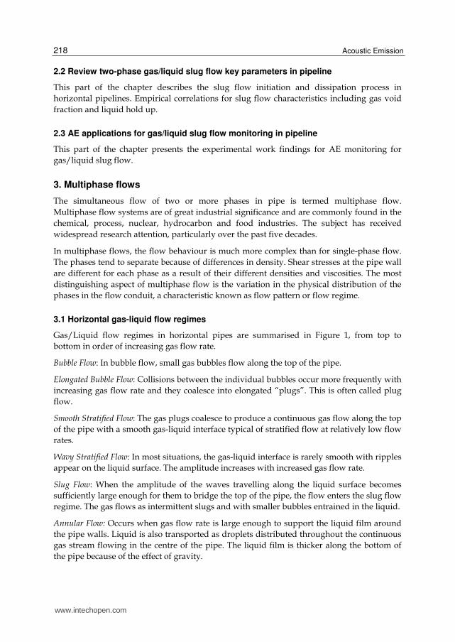
Gas/Liquid flow regimes in horizontal pipes are summarised in Figure 1, from top to

bottom in order of increasing gas flow rate.

Bubble Flow: In bubble flow, small gas bubbles flow along the top of the pipe.

Elongated Bubble Flow: Collisions between the individual bubbles occur more frequently with

increasing gas flow rate and they coalesce into elongated “plugs”. This is often called plug

flow.

Smooth Stratified Flow: The gas plugs coalesce to produce a continuous gas flow along the top

of the pipe with a smooth gas-liquid interface typical of stratified flow at relatively low flow

rates.

Wavy Stratified Flow: In most situations, the gas-liquid interface is rarely smooth with ripples

appear on the liquid surface. The amplitude increases with increased gas flow rate.

Slug Flow: When the amplitude of the waves travelling along the liquid surface becomes

sufficiently large enough for them to bridge the top of the pipe, the flow enters the slug flow

regime. The gas flows as intermittent slugs and with smaller bubbles entrained in the liquid.

Annular Flow: Occurs when gas flow rate is large enough to support the liquid film around

the pipe walls. Liquid is also transported as droplets distributed throughout the continuous

gas stream flowing in the centre of the pipe. The liquid film is thicker along the bottom of

the pipe because of the effect of gravity.

www.intechopen.com

Upstream Multiphase Flow Assurance Monitoring Using Acoustic Emission 219

Fig. 1. Flow regimes of gas/ liquid horizontal flow

3.2 Gas-liquid flow regimes map in horizontal flow

The most distinguish aspect of multi-phase flow is the variation of the physical distribution of the phases in the flow conduit, a characteristic known as flow pattern or flow regime. The flow pattern that exists depends on the relative magnitudes of the forces that act on the fluids. These forces such as buoyancy, turbulence, inertia, and surface-tension forces, all vary significantly with flow rates, pipe diameter, inclination angle, and fluid properties of the phases.

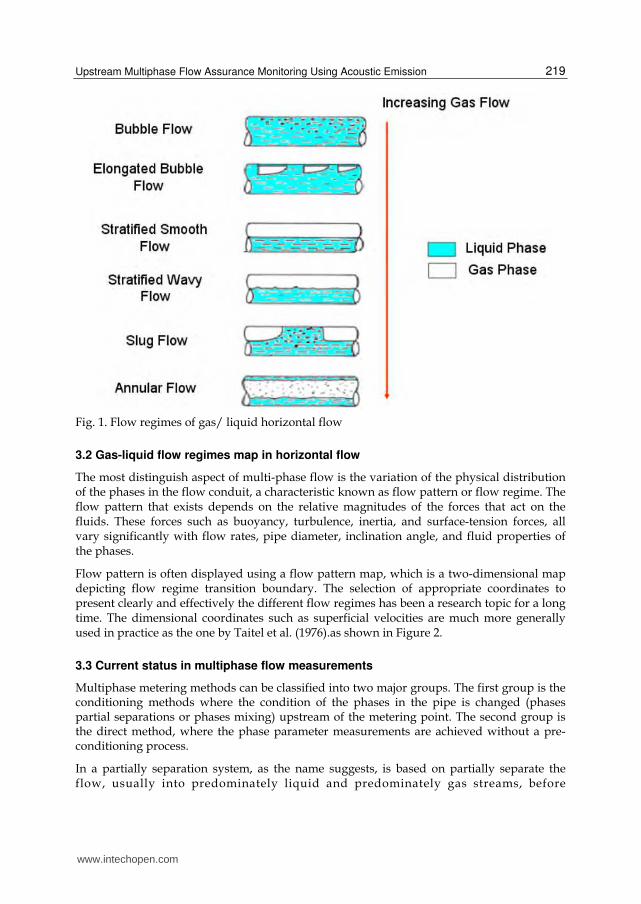
Flow pattern is often displayed using a flow pattern map, which is a two-dimensional map depicting flow regime transition boundary. The selection of appropriate coordinates to present clearly and effectively the different flow regimes has been a research topic for a long time. The dimensional coordinates such as superficial velocities are much more generally used in practice as the one by Taitel et al. (1976).as shown in Figure 2.

3.3 Current status in multiphase flow measurements

Multiphase metering methods can be classified into two major groups. The first group is the conditioning methods where the condition of the phases in the pipe is changed (phases partial separations or phases mixing) upstream of the metering point. The second group is the direct method, where the phase parameter measurements are achieved without a pre-conditioning process.

In a partially separation system, as the name suggests, is based on partially separate the flow, usually into predominately liquid and predominately gas streams, before

www.intechopen.com


Fig. 2. Horizontal flow regimes map by Taitel et al. (1976)

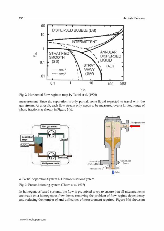
measurement. Since the separation is only partial, some liquid expected to travel with the

gas stream. As a result, each flow stream only needs to be measured over a limited range of

phase fractions as shown in Figure 3(a).

a. Partial Separation System b. Homogenisation System

Fig. 3. Preconditioning system (Thorn et al. 1997)

In homogenous based systems, the flow is pre-mixed to try to ensure that all measurements

are made on a homogenous flow, hence removing the problem of flow regime dependency

and reducing the number of and difficulties of measurement required. Figure 3(b) shows an

www.intechopen.com


example of a commercially available three-phase flowmeter which uses this strategy. The

Framo multiphase flowmeter uses a tank mixer to homogenize the flow both radially and

axially. The homogenized flow then passes through a Venturi meter which is used to

measure the velocity of the mixture, and a dual-energy-ray attenuation meter which uses

two different energy levels of the Barium 133 isotope to determine the oil, water and gas

fractions.

3.4 Measurement strategies – inferential approach

The primary information required by a user of multiphase meters is the mass flow rate of

the each phase. An ideal multiphase flow meter would make independent direct

measurements of each of these quantities. Unfortunately, direct mass flowmeters for use

with two phase flows are rare and do not exist at all for three phase flows.

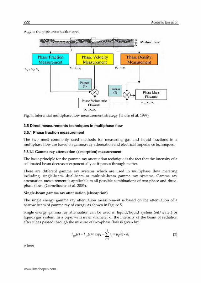
An alternative to direct mass flow measurement is to use an inferential method. An

inferential mass method requires both the instantaneous velocity and cross sectional fraction

of each component to be know in order to calculate the individual component mass

flowrates and total mixture mass flowrate (Thorn et al. 1997). Figure 4 shows a schematic of

such an approach.

Two types of parameters are monitored by a multiphase metering system:

1. Primary parameters:

Phase fraction (e.g. void fraction, water cut);

Phase velocity (the velocity of each phase as they cannot be assumed to be

travelling at the same velocity);

Phase density.

2. Secondary parameters:

Flow regime (this may be considered as a primary parameter if a flow dependent

sensing technique is used);

Phase viscosity;

Phase salinity;

Phase permittivity/ conductivity.

Density information of the oil, water and gas components are readily available from other

parts of the production process, e.g. densitometer readings or estimated from PVT diagrams

using measured pressure and temperature. Therefore, the problem is to measure the oil,

water, and gas velocities and two of the component fractions. The third component fraction

(oil fraction) is deduced from the fact that the sum of the three phase fractions is equal to

unity.

g g g pipe w w w pipe o o o pipem α V ρ A α V ρ A α V ρ A (1)

where

m is the total mass flow rate,

g w oρ ,ρ and ρ are the densities of gas, water and oil, Vg, Vw and Vo are the velocities of gas, water and oil,

www.intechopen.com


Apipe is the pipe cross section area.

Fig. 4. Inferential multiphase flow measurement strategy (Thorn et al. 1997)

3.5 Direct measurements techniques in multiphase flow

3.5.1 Phase fraction measurement

The two most commonly used methods for measuring gas and liquid fractions in a

multiphase flow are based on gamma-ray attenuation and electrical impedance techniques.

3.5.1.1 Gamma ray attenuation (absorption) measurement

The basic principle for the gamma-ray attenuation technique is the fact that the intensity of a

collimated beam decreases exponentially as it passes through matter.

There are different gamma ray systems which are used in multiphase flow metering

including, single-beam, dual-beam or multiple-beam gamma ray systems. Gamma ray

attenuation measurement is applicable to all possible combinations of two-phase and three-

phase flows (Corneliussen et al. 2005).

Single-beam gamma ray attenuation (absorption)

The single energy gamma ray attenuation measurement is based on the attenuation of a

narrow beam of gamma ray of energy as shown in Figure 5.

Single energy gamma ray attenuation can be used in liquid/liquid system (oil/water) or

liquid/gas system. In a pipe, with inner diameter d, the intensity of the beam of radiation

after it has passed through the mixture of two-phase flow is given by:

2

i 1

I (e) I (e) exp[ α ┤ (e) d]m ┥ i i (2)

where

www.intechopen.com


Fig. 5. Single-beam gamma ray densitometer

I (e)m is the measured countrate,

┥I (e) is the count rate when the pipe is empty,

┤i is the linear attenuation coefficients for the two phases.

Apart from fractions of the phases iα , the attenuation coefficients ┤i are also initially

unknown. However, the latter can be found by calibration where the meter is filled with individual fluids. In both cases the following two equations for water and oil can be used:

I I exp[ α ┤ d]w ┥ w w (3)

I I exp[ α ┤ d]o ┥ o o (4)

These two calibration points together with the relation α α 1w o can be rewritten as an expression for the water fraction in two-phase liquid/liquid mixture (or the water cut):

ln(I ) ln(I )w mαw ln(I ) ln(I )w o

(5)

Dual-energy gamma ray attenuation (absorption)

In order to determine oil, water and gas fractions, two independent measurements are required using dual or multiple energy technique. This technique has been investigated by a number of researchers (Abouelawafa and Kendall. 1980; Roach and Watt. 1996; Van Santen et al. 1995 and Hewitt et al. 1995).

The basics of dual energy gamma ray absorption measurement are similar to the single energy gamma ray attenuation concept, but now two gamma energies e1 and e2 are used. In

BEAM

Fan Beam Lead Collimator

Source

Detector

Pre-amplifier

Count rate

Output

Signal-Channel

Analysers

Test-Section

(Incident) )ln(I0

(gas) )ln(Ig

(oil) )ln(Io

(water) )ln(Iw

)ln(I

Distance from Source

www.intechopen.com


a pipe, with inner diameter d, containing a mixture of water, oil and gas with fractionsα , α and αg w o , the measured count rate I (e)m

is:

3

i 1

I (e) I (e) exp[ α ┤ (e) d]m ┥ i i (6)

where

I (e)┥ is the count rate when the pipe is empty,

i is represent the linear attenuation coefficients for the three phases ( ┤ ,┤ ,┤g w o ).

For two energy levels, e1 and e2, provided the linear attenuation coefficients between water, oil, and gas are sufficiently different, two independent equations are obtained. The third equation is simply the fact that the sum of the three phase fractions in closed conduit should equal to unity as given:

α α α 1g w o (7)

A full set of linear equations is given below. RO, RW, Rg, and Rm represent the logarithm of the count rates for water, oil, gas and mixture, respectively, at energies e1 and e2.

R (e ) R (e ) R (e ) α R (e ) w 1 o 1 g 1 w m 1R (e ) R (e ) R (e ) α R (e ) w 2 o 2 g 2 o m 2

α 11 1 1 g

(8)

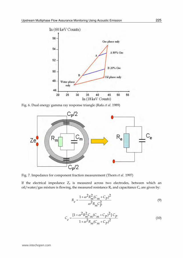
The elements in the matrix are determined in a calibration process by filling the pipe with 100% water, 100% oil, and 100% gas (air) or alternatively by calculations based on the fluid properties. Together with the measured count rates at the two energy levels from a multiphase mixture it is possible to calculate the unknown phase fractions. In Figure 6 shows a typical response triangle with a dual energy source (18 keV and 60 keV) for water, oil and gas mixture.

The corners of the triangle are the water, oil and gas calibrations, and any point inside this triangle represents a particular composition of water, oil and gas (Rafa et al. 1989). The shape of the triangle depends mainly on the energy levels used (thus specific radioactive source), pipe diameter and detector characteristics; however, fluid properties may also influence the triangular shape. If the count levels are too close the triangle will transform into a line and therefore cannot be used for a three-phase composition measurement.

3.5.1.2 Electrical impedance measurements

The main principle of electrical impedance methods for component fraction measurements is that the fluid flowing in the measurement section of the pipe is characterised as an electrical conductor. By measuring the electrical impedance across the pipe diameter (using e.g. contact or non-contact electrodes), properties of the fluid mixture, conductance and capacitance, can be determined. The measured electrical quantity of the mixture then depends on the conductivity and permittivity of the oil, gas and water components, respectively. Figure 7 shows the basic principle of impedance method to measure component fraction.

www.intechopen.com


Fig. 6. Dual energy gamma ray response triangle (Rafa et al. 1989)

Fig. 7. Impedance for component fraction measurement (Thorn et al. 1997)

If the electrical impedance Ze is measured across two electrodes, between which an

oil/water/gas mixture is flowing, the measured resistance Re and capacitance Ce are given by:

R C Cm m PRe

R Cm P

2 2 21 ( )

2 2

(9)

R C C C Cm m m P PCe

R C Cm m P

2 2 2[1 ( ) ]

2 21 ( )

(10)

www.intechopen.com


The resistance Rm and capacitance Cm of the mixture flowing through the pipe depends on

the permittivity and conductivity of the oil, water and gas components, the void fraction

and water fraction of the flow, and the flow regime.

The measured resistance and capacitance not only depends on Rm and Cm but also on the

excitation frequency of the detection electronics and the geometry and materials of the

sensor. For a particular sensor geometry (and hence fixed CP) and flow regime, the

measured impedance will be a direct function of the flow component ratio.

In oil continuous mixture Re is large and can be difficult to measure reliably. For the flows in

which water is the continuous phase, a short circuiting effect will occur, caused by the

conductive water, if the sensor excitation frequency, fc, is less than:

wfc 2 o w

(11)

where

w w and are the conductivity and permittivity of the water component respectively.

For process water this would mean a frequency below that of microwave frequencies.

Therefore, impedance method is limited to oil or water in continuous phase.

However impedance based methods suffer from two important limitations - they cannot be

used over the full component fraction range and are flow regime dependent. This

dependency is eliminated by one of two methods: (1) homogenisation of the phase, before

the measurement is made and (2) development of electrodes which minimise the

dependency upon the flow geometry.

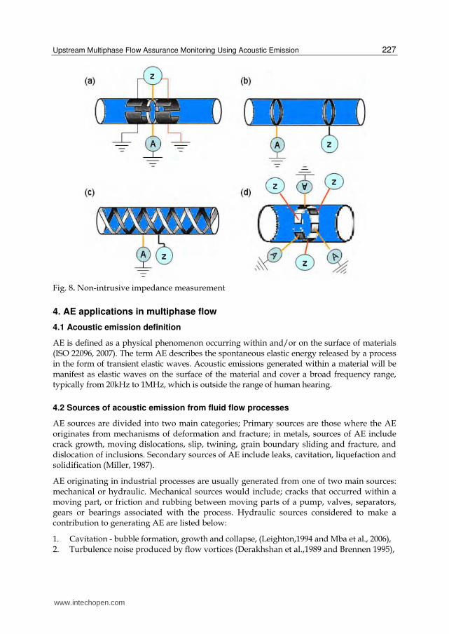
Various methods have been used to reduce the flow regime dependency effects of

impedance sensors as shown in Figure 8. In this figure four different designs of non-

intrusive sensor are illustrated. These styles have been developed recently, and that to

minimise the flow geometry dependency,

Arc electrodes, (Xie et al. 1990), for resistive and capacitive cross-section measurement,

Figure 8 (a). In this design the guard electrodes are installed at either side of the electrodes,

in order to reduce the sensitivity to axial flow distributions.

Ring electrodes (Andreussi et al. 1988), for resistive measurement and to achieve a uniform

electric field structure within the sensing volume, the ring electrodes trade-off a localised

cross-section measurement. Figure 8 (b).

Helical electrodes (Abouelwafa and Kendall. 1980), Figure 8 (c). In this model, the electrodes

twist round the pipe, to overcome flow geometry dependence.

Rotating field electrodes (Merilo et al. 1977), as shown in Figure 8 (d), this design achieves a

similar effect to helical electrodes. Here, three electrode pairs are driven at 120 phase

intervals, to produce a rotating field vector in the pipe centre.

www.intechopen.com


Fig. 8. Non-intrusive impedance measurement

4. AE applications in multiphase flow

4.1 Acoustic emission definition

AE is defined as a physical phenomenon occurring within and/or on the surface of materials (ISO 22096, 2007). The term AE describes the spontaneous elastic energy released by a process in the form of transient elastic waves. Acoustic emissions generated within a material will be manifest as elastic waves on the surface of the material and cover a broad frequency range, typically from 20kHz to 1MHz, which is outside the range of human hearing.

4.2 Sources of acoustic emission from fluid flow processes

AE sources are divided into two main categories; Primary sources are those where the AE originates from mechanisms of deformation and fracture; in metals, sources of AE include crack growth, moving dislocations, slip, twining, grain boundary sliding and fracture, and dislocation of inclusions. Secondary sources of AE include leaks, cavitation, liquefaction and solidification (Miller, 1987).

AE originating in industrial processes are usually generated from one of two main sources: mechanical or hydraulic. Mechanical sources would include; cracks that occurred within a moving part, or friction and rubbing between moving parts of a pump, valves, separators, gears or bearings associated with the process. Hydraulic sources considered to make a contribution to generating AE are listed below:

1. Cavitation - bubble formation, growth and collapse, (Leighton,1994 and Mba et al., 2006), 2. Turbulence noise produced by flow vortices (Derakhshan et al.,1989 and Brennen 1995),

www.intechopen.com


3. Gas, solid and liquid mixture interaction in multiphase flows,(Boyd and Varley 2001) 4. Flow past restrictions and side branches in piping systems (McNulty, 1985), 5. Broadband turbulence energy resulting from high flow velocities, (McNulty, 1985), 6. Intermittent bursts of broadband energy caused by cavitation, flashing, recirculation,

and water hammer (Neill et al., 1998), 7. Liquid drops impacting on a liquid surface (rain fall) (Pumphrey and Crum, 1989; Oguz

and Prosperetti,1990), 8. Leakage from e.g. pipes (Lee and Lee, 2006), 9. Chemical reactions (Van Ooijen et al., 1978), 10. Foam break up (Lubetkin, 1989), and 11. Oceanic noise due to the breaking of waves (Leighton,1994 ;Vergniolle et al., 1996;

Grant 1997)

In the above list, the AE emitted from liquid flow as a direct consequence of gas bubble formation and collapse is an important area for search, even though each source has a different formation mechanism.

4.3 The mechanisms of acoustic emission and sound generated from bubbles

In the literature the earliest known reference relating to the sound emitted from water/air mixtures due to the presence of air bubbles was by Bragg (1921); the murmuring of a brook and the "plunk" of liquid droplets impacting on the water surface were both attributed to entrained air bubbles. The first person to relate the frequency of the sound produced by a bubble formed at a nozzle to the physical parameters involved was Minnaert (1933). Subsequently, a number of investigations were devoted to the sound emitted from two phase flow as a function of bubble size and bubble population, Schiebe (1969), Pandit et al., (1992), Terrill and Melville (2000), Manasseh et al., (2001) and Al-Masry et al., (2005).

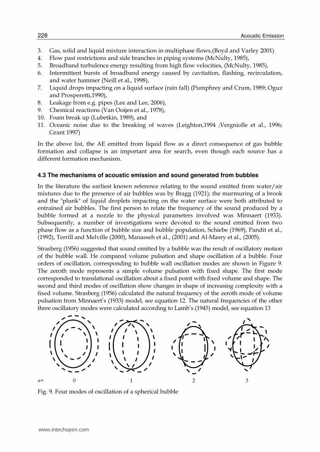
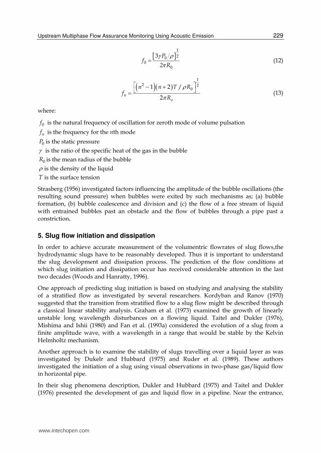
Strasberg (1956) suggested that sound emitted by a bubble was the result of oscillatory motion of the bubble wall. He compared volume pulsation and shape oscillation of a bubble. Four orders of oscillation, corresponding to bubble wall oscillation modes are shown in Figure 9. The zeroth mode represents a simple volume pulsation with fixed shape. The first mode corresponded to translational oscillation about a fixed point with fixed volume and shape. The second and third modes of oscillation show changes in shape of increasing complexity with a fixed volume. Strasberg (1956) calculated the natural frequency of the zeroth mode of volume pulsation from Minnaert’s (1933) model, see equation 12. The natural frequencies of the other three oscillatory modes were calculated according to Lamb’s (1945) model, see equation 13

n= 0 1 2 3

Fig. 9. Four modes of oscillation of a spherical bubble

www.intechopen.com


P

f2 R

1

200

0

3 (12)

no

n n T Rf

R

12 2

01 2 /

2

(13)

where:

f0 is the natural frequency of oscillation for zeroth mode of volume pulsation

nf is the frequency for the nth mode

P0 is the static pressure

is the ratio of the specific heat of the gas in the bubble

R0 is the mean radius of the bubble

is the density of the liquid

T is the surface tension

Strasberg (1956) investigated factors influencing the amplitude of the bubble oscillations (the resulting sound pressure) when bubbles were exited by such mechanisms as; (a) bubble formation, (b) bubble coalescence and division and (c) the flow of a free stream of liquid with entrained bubbles past an obstacle and the flow of bubbles through a pipe past a constriction.

5. Slug flow initiation and dissipation

In order to achieve accurate measurement of the volumentric flowrates of slug flows,the hydrodynamic slugs have to be reasonably developed. Thus it is important to understand the slug development and dissipation process. The prediction of the flow conditions at which slug initiation and dissipation occur has received considerable attention in the last two decades (Woods and Hanratty, 1996).

One approach of predicting slug initiation is based on studying and analysing the stability of a stratified flow as investigated by several researchers. Kordyban and Ranov (1970) suggested that the transition from stratified flow to a slug flow might be described through a classical linear stability analysis. Graham et al. (1973) examined the growth of linearly unstable long wavelength disturbances on a flowing liquid. Taitel and Dukler (1976), Mishima and Ishii (1980) and Fan et al. (1993a) considered the evolution of a slug from a finite amplitude wave, with a wavelength in a range that would be stable by the Kelvin Helmholtz mechanism.

Another approach is to examine the stability of slugs travelling over a liquid layer as was investigated by Dukelr and Hubbard (1975) and Ruder et al. (1989). These authors investigated the initiation of a slug using visual observations in two-phase gas/liquid flow in horizontal pipe.

In their slug phenomena description, Dukler and Hubbard (1975) and Taitel and Dukler (1976) presented the development of gas and liquid flow in a pipeline. Near the entrance,

www.intechopen.com


the gas tends to flow above a moving stratified liquid layer. However, because of the shear forces created at the pipe wall, the liquid layer tends to decelerate as it moves along the pipe and its height changes gradually towards an equilibrium height which is governed by the pressure force, shear and gravitational forces.

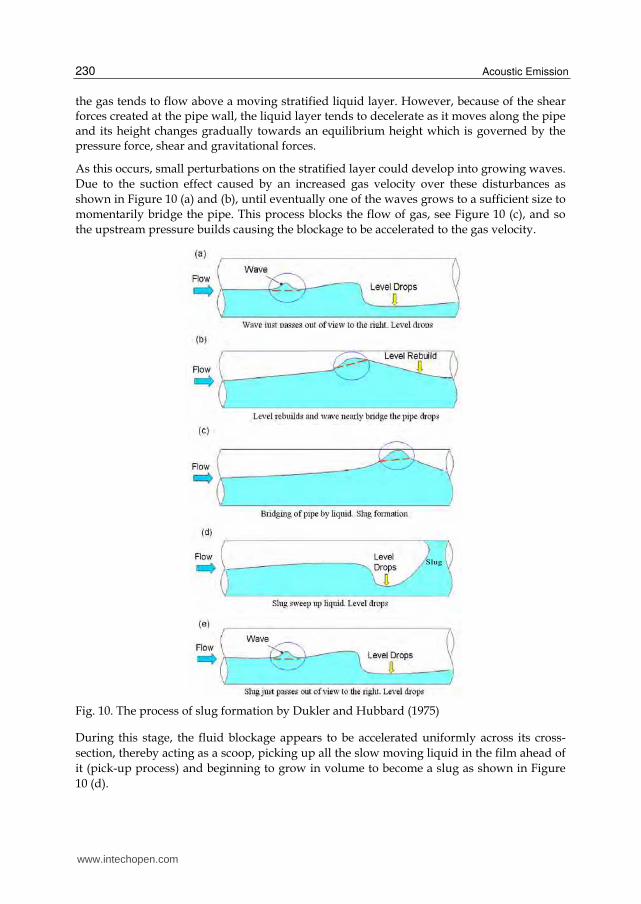
As this occurs, small perturbations on the stratified layer could develop into growing waves.

Due to the suction effect caused by an increased gas velocity over these disturbances as

shown in Figure 10 (a) and (b), until eventually one of the waves grows to a sufficient size to

momentarily bridge the pipe. This process blocks the flow of gas, see Figure 10 (c), and so

the upstream pressure builds causing the blockage to be accelerated to the gas velocity.

Fig. 10. The process of slug formation by Dukler and Hubbard (1975)

During this stage, the fluid blockage appears to be accelerated uniformly across its cross-

section, thereby acting as a scoop, picking up all the slow moving liquid in the film ahead of

it (pick-up process) and beginning to grow in volume to become a slug as shown in Figure

10 (d).

Slug

www.intechopen.com


Gas may also be entrained in the form of small bubbles, which are deformed by the combined effect of buoyancy forces and the turbulent shear forces created by velocity differences between the slug front and the liquid film. As a result, a dispersion of small bubbles is often produced which may be transported through the body of the liquid slug.

Meanwhile, at the slug tail, liquid and previously entrained gas are released (shedding process) from the slug body. The “shed” liquid decelerates to a velocity determined by the shear stresses at the wall and the interface and becomes a stratified layer as illustrated in Figure 10 (e). The “shed” gas mainly passes into the elongated bubble region above this layer, although a fraction may remain entrained within the liquid film.

As long as the volumetric “pick-up” rate is larger than the “shedding” rate, the slug continues to grow. However, eventually the “pick-up” rate becomes equal to the “shedding” rate and the slug becomes fully developed so that the slug length stabilises. Nydal et al. (1992) experimentally investigated the length of the pipe required to reach quasi-stable flow conditions (slug development distance) and found that it is between 300 and 600 pipe diameters. Once the quasi-stable conditions are reached, the slug length has a mean value between 12 to 15 pipe diameters.

Based on the shedding and pick-up processes, slug flow might be classified into three main states. The pick-up rate is greater than the shedding rate; the slug in this case continues to grow. The “pick-up” rate equals to the “shedding” rate, the slug becomes fully developed so that the slug length stabilises. Finally, when the “pick-up” rate is less than the “shedding” rate, the slug under this condition dissipates.

The slug dissipation process occurs as the gas flowrate and consequently the slug velocity and the degree of aeration of the slug increases. Ultimately the gas forms a continuous phase through the slug body. When this occurs the slug begins bypassing some of the gas. At this point the slug no longer maintains a competent bridge to block the gas flow so the characteristics of the flow changes. This point is the beginning of “blow-though” and the start of the annular flow regime.

The idealised picture of a “stable slug” flow in horizontal pipe is presented in figure 11. The section ‘F’ represents the front region of the liquid slug body (LSB) and section ‘T’ represent the tail region of the liquid slug body. In a stable slug flow, the liquid slug body length, LLSB and the elongated bubble (EB) length (LEB) remain essentially constant in the downstream direction.

Fig. 11. Schematic description of the EB and LSB in idealised developed slug flow

LEBLLSB

Liquid Slug Body (LSB) Elongated Bubble (EB)

HLF

VT

VGEB

VLF

VLSB(G)

VLSB(L)ФGT

ФGE

ФGB

FT

EB noseEB tail

LEBLLSB

Liquid Slug Body (LSB) Elongated Bubble (EB)

HLF

VT

VGEB

VLF

VLSB(G)

VLSB(L)ФGT

ФGE

ФGB

FT

EB noseEB tail

www.intechopen.com


The gas in the elongated bubble moves at a velocity, VGEB, which is faster than the average mixture velocity, Vmix in the liquid slug body. As a result, the liquid is shed from the back of the liquid slug body to form the liquid film layer along the elongated bubble. The liquid in the film at the EB nose may be aerated. Also, bubbles in the liquid slug body coalesce with the elongated bubble interface and are gradually absorbed, which in the fullness of time results in the liquid film becoming un-aerated. The mixture velocity is the sum of the liquid velocity and the gas velocity (VSL + VSG).

At the same time, the gas bubbles are fragmented from the tail of the elongated bubble and re-entrained into the front section of liquid slug body ‘F’ at a rate ФGE. The fragmentation of the elongated bubble tail and the entrainment of the bubbles into the front section of the liquid slug body are due to the dispersing forces induced by the flow of the liquid film as it plunges into the liquid slug front. However, some of the gas bubbles that are entrained into the front section of the liquid slug body may re-coalesce with the elongated bubble tail at ФGB rate, resulting in a net gas flow rate of ФGE - ФGB out of the elongated bubble tail. The ФGT= ФGE - ФGB is the constant gas flow rate which is entrained to the elongated bubble EB, and eventually is absorbed into the successive elongated bubble. Therefore, the net rate of gas entrainment in the slug body is the result of a balance between bubble injection and rejection.

The gas bubbles entrainment from the elongated bubble tail and their re-coalescence at the successive nose result in an effective elongated bubble translation velocity, VT, which is higher than the gas velocity in the elongated bubble, VGEB. From the description of the slug flow formation, dispersed gas bubbles can be generated in the liquid slug body region through the formation, coalescence, breakage and collapse of bubbles processes. The entrained gas bubbles in the liquid experience a transient pressure as they move through the hydrodynamic pressure field of the liquid. The transient pressure causes the gas bubbles to oscillate at their natural frequencies; one consequence of which is the generation of sound (Strasberg, 1956).

5.1 Gas void fraction ( ) in slug flow

The liquid holdup in the slug body or gas void fraction ( ) is an important parameter for

the design of multiphase pipelines and associated separation equipment. The definition of

the liquid holdup is “the flowrate of the liquid phase divided by the total flowrate of both

the gas and liquid flowrates”. And the definition of the gas void fraction is “the flowrate of

the gas phase divided by the total flowrate of both the gas and liquid flowrates”. Several gas

void fraction correlations were developed, however, the majority of these correlations were

obtained based on the slug body liquid holdup. In multiphase flow, the extensively-used

correlation developed by Gregory et al. (1978) was obtained from the measurements of

liquid holdup, using electrical capacitance probes, in air-water and oil-water flow in

horizontal pipes with diameter of 0.0258 m and 0.0512 m. The correlation gives slug body

holdup as a function of the mixture velocity Vmix only:

LSB

mix

1H

V1

8.66

1.39

(14)

www.intechopen.com


where Vmix is the slug mixture velocity in ms-1 and is equal to the sum of the superficial gas

and liquid velocities.

Malnes (1982) proposed an alternative correlation also based on the same data of Gregory et

al. (1978) as:

mixLSB

C mix

VH

C V1 (15)

Where, the dimensional coefficient Cc is measured as following:

C

gC

L

0.25

83

(16)

Beggs and Brill, (1973) developed their correlation for the whole spectrum of flow situations

using 1” and 1.5” pipe sizes at various angles from the horizontal. The correlation passed on

Froude number and the slug body length for the intermittent flow as following;

LSBE

Fr

0.5351

0.0173

0.845 (17)

where Fr is the Froude number, defined as a dimensionless number comparing inertia and

gravitational forces, and calculated as

mixVFr

gD

2 (18)

Hughmark (1962) proposed correlation for the gas void fraction based on slug mixture

velocity and superficial gas velocity, given by:

SG

mix

V

V1.2 (19)

Gregory and Scott (1969), developed similar correlation to the one proposed by Hughmark

(1962), as following:

SG

mix

V

V1.19 (20)

Ferschneider (1983) developed a more complex correlation for slug body holdup HLSB using

data obtained from natural gas and a light hydrocarbon oil facility. The facility loop

comprised a 0.15 m diameter with 120 m long test section loop and operated at elevated

pressure of between 10 and 50 bar. The correlation proposed by Ferschneider (1983) took

account for surface tension of the fluids in terms of Bond number (Bo). Bo is a measure of

the importance of the surface tension forces compared to gravitational forces.

www.intechopen.com


LSB 22

0.1mix

G

L

1H

V Bo1

25ρ1 gDρ

(21)

Bo is Bond number and is given by:

2

L Gρ ρ g DBo

σ (22)

Nickline (1962) proposed correlation for the gas void fraction based on the measured liquid

holdup for air-water flow in 0.05m and 0.09 m horizontal pipe. The correlation is given by

the expressions:

SG

mix

V

V gD(1.2 0.35 (23)

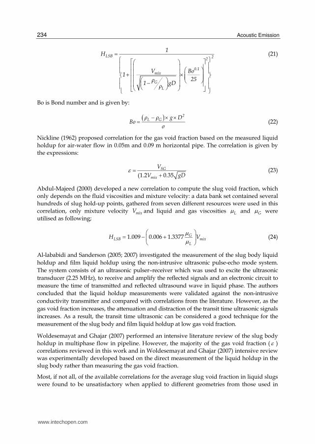
Abdul-Majeed (2000) developed a new correlation to compute the slug void fraction, which

only depends on the fluid viscosities and mixture velocity: a data bank set contained several

hundreds of slug hold-up points, gathered from seven different resources were used in this

correlation, only mixture velocity mixV and liquid and gas viscosities L and G were

utilised as following;

GLSB mix

L

H V1.009 0.006 1.3377

(24)

Al-lababidi and Sanderson (2005; 2007) investigated the measurement of the slug body liquid

holdup and film liquid holdup using the non-intrusive ultrasonic pulse-echo mode system.

The system consists of an ultrasonic pulser–receiver which was used to excite the ultrasonic

transducer (2.25 MHz), to receive and amplify the reflected signals and an electronic circuit to

measure the time of transmitted and reflected ultrasound wave in liquid phase. The authors

concluded that the liquid holdup measurements were validated against the non-intrusive

conductivity transmitter and compared with correlations from the literature. However, as the

gas void fraction increases, the attenuation and distraction of the transit time ultrasonic signals

increases. As a result, the transit time ultrasonic can be considered a good technique for the

measurement of the slug body and film liquid holdup at low gas void fraction.

Woldesemayat and Ghajar (2007) performed an intensive literature review of the slug body

holdup in multiphase flow in pipeline. However, the majority of the gas void fraction ( )

correlations reviewed in this work and in Woldesemayat and Ghajar (2007) intensive review

was experimentally developed based on the direct measurement of the liquid holdup in the

slug body rather than measuring the gas void fraction.

Most, if not all, of the available correlations for the average slug void fraction in liquid slugs

were found to be unsatisfactory when applied to different geometries from those used in

www.intechopen.com


extracting the empirical correlations (Paglianti et al., 1993).This is perhaps not surprising

since the above mentioned correlations are derived from fully developed slug flow, and do

not account for the transient behaviour of slug growth and collapse (Bonizzi and Issa, 2003).

6. AE applications for multiphase slug flow monitoring in pipelines

6.1 Experimental setup

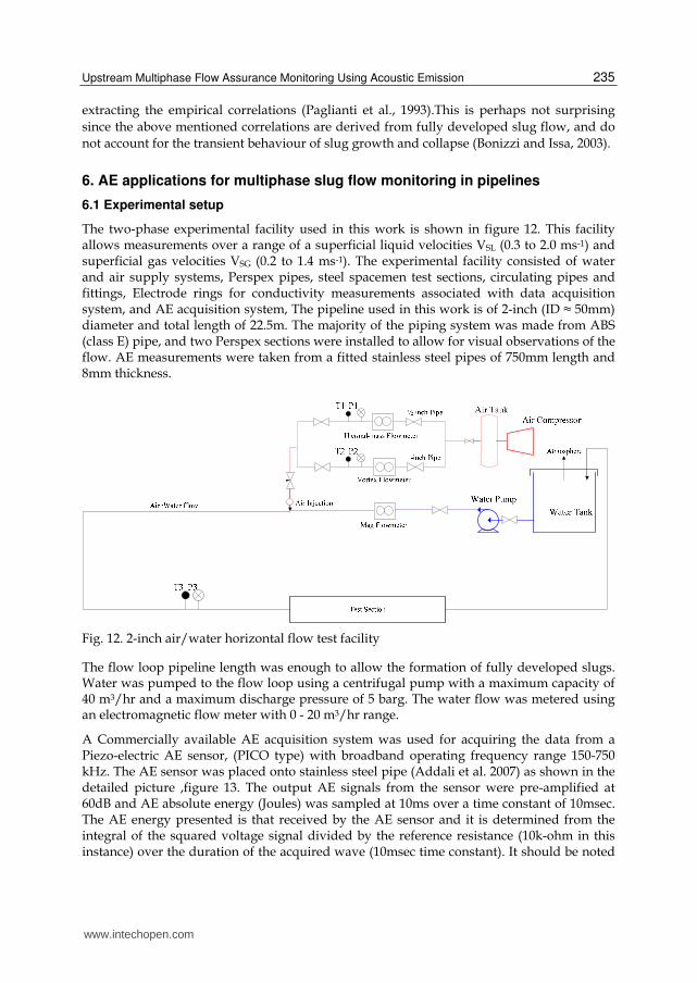
The two-phase experimental facility used in this work is shown in figure 12. This facility allows measurements over a range of a superficial liquid velocities VSL (0.3 to 2.0 ms-1) and superficial gas velocities VSG (0.2 to 1.4 ms-1). The experimental facility consisted of water and air supply systems, Perspex pipes, steel spacemen test sections, circulating pipes and fittings, Electrode rings for conductivity measurements associated with data acquisition system, and AE acquisition system, The pipeline used in this work is of 2-inch (ID ≈ 50mm) diameter and total length of 22.5m. The majority of the piping system was made from ABS (class E) pipe, and two Perspex sections were installed to allow for visual observations of the flow. AE measurements were taken from a fitted stainless steel pipes of 750mm length and 8mm thickness.

Fig. 12. 2-inch air/water horizontal flow test facility

The flow loop pipeline length was enough to allow the formation of fully developed slugs. Water was pumped to the flow loop using a centrifugal pump with a maximum capacity of 40 m3/hr and a maximum discharge pressure of 5 barg. The water flow was metered using an electromagnetic flow meter with 0 - 20 m3/hr range.

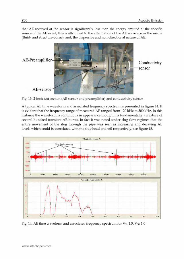
A Commercially available AE acquisition system was used for acquiring the data from a Piezo-electric AE sensor, (PICO type) with broadband operating frequency range 150-750 kHz. The AE sensor was placed onto stainless steel pipe (Addali et al. 2007) as shown in the detailed picture ,figure 13. The output AE signals from the sensor were pre-amplified at 60dB and AE absolute energy (Joules) was sampled at 10ms over a time constant of 10msec. The AE energy presented is that received by the AE sensor and it is determined from the integral of the squared voltage signal divided by the reference resistance (10k-ohm in this instance) over the duration of the acquired wave (10msec time constant). It should be noted

www.intechopen.com


that AE received at the sensor is significantly less than the energy emitted at the specific source of the AE event; this is attributed to the attenuation of the AE wave across the media (fluid- and structure-borne), and, the dispersive and non-directional nature of AE.

Fig. 13. 2-inch test section (AE sensor and preamplifier) and conductivity sensor

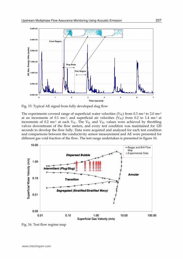
A typical AE time waveform and associated frequency spectrum is presented in figure 14. It

is evident that the frequency range of measured AE ranged from 120 kHz to 500 kHz. In this

instance the waveform is continuous in appearance though it is fundamentally a mixture of

several hundred transient AE bursts. In fact it was noted under slug flow regimes that the

entire movement of the slug through the pipe was seen as increasing and decaying AE

levels which could be correlated with the slug head and tail respectively, see figure 15.

Fig. 14. AE time waveform and associated frequency spectrum for VSL 1.5, VSG 1.0

Slug body passingSlug body passing

www.intechopen.com


Fig. 15. Typical AE signal from fully developed slug flow

The experiments covered range of superficial water velocities (VSL) from 0.3 ms-1 to 2.0 ms-1 at an increments of 0.1 ms-1; and superficial air velocities (VSG) from 0.2 to 1.4 ms-1 at increments of 0.2 ms-1 at each VSL. The VSL and VSG values were achieved by throttling valves downstream of the flow meters, and every test condition was maintained for 120 seconds to develop the flow fully. Data were acquired and analysed for each test condition and comparisons between the conductivity sensor measurement and AE were presented for different gas void fraction of the flow. The test range undertaken is presented in figure 16.

Fig. 16. Test flow regime map

0.00E+00

5.00E+02

1.00E+03

1.50E+03

2.00E+03

2.50E+03

3.00E+03

0 1 2 3 4 5 6 7

Time (second)

AE

Ab

s.

En

erg

y (

Att

o j

ou

les

)

Film Region

Slug Body

Front Region

0.00

0.01

0.10

1.00

10.00

0.01 0.10 1.00 10.00 100.00Superficial Gas Velocity (m/s)

Su

pe

rfic

ial W

ate

r V

elo

city (

m/s

)

Beggs and Brill FlowMapExperimental Data

Segregated (Stratified/Stratified Wavy)

Transition

Annular

Intermittent (Plug/Slug)

Dispersed Bubble

0.00

0.01

0.10

1.00

10.00

0.01 0.10 1.00 10.00 100.00Superficial Gas Velocity (m/s)

Su

pe

rfic

ial W

ate

r V

elo

city (

m/s

)

Beggs and Brill FlowMapExperimental Data

Segregated (Stratified/Stratified Wavy)

Transition

Annular

Intermittent (Plug/Slug)

Dispersed Bubble

www.intechopen.com


6.2 Result and discussion

6.2.1 Gas bubbles in slug body

In the liquid slug body, a gas bubble in the liquid slug body will be broken down by the turbulent forces exerted on it if its size is larger than a certain value, this value known as the ‘Kolmogorov’ length scale (Kolmogorov,1949). Based on the extension of Kolmogorov–Hinze theory (Hinze, 1955) for break-up of droplets/bubbles in a turbulent field, several correlations for gas void fraction in the slug body were developed (Barnea & Brauner, 1985; Brauner, 2001; Brauner & Ullmann, 2002). From the Kolmogorov–Hinze theory, the amount of gas bubbles a liquid slug body can hold is dependent on the turbulent intensity of the liquid phase. Therefore, there must be a balance between the total surface free energy of dispersed gas bubbles and the turbulent kinetic energy of the liquid phase.

Adamson,(Adamson, 1990) stated that the surface free energy per unit interfacial area is the work necessary to generate this area, and is equal to the interfacial surface tension between a liquid phase and a gas phase. Assuming gas bubbles are all spherical with a diameter of dbubble, the total surface free energy of the discrete gas bubbles (Esurface) in the liquid slug body was developed by Brauner and Ulmann (Brauner & Ullmann, 2004) as:

surface i LSB LSB

bubble

6σE A (1 H ) L

d (25)

where σ is the interfacial surface tension, Ai is the internal cross-sectional area of the pipe, HLSB is the liquid holdup in the slug body, and LLSB is the length of the liquid slug body. In slug flow, the gas phase is accommodated in the liquid slug body as dispersed spherical bubbles. Brodkey (Brodkey, 1967) noted a critical bubble diameter, dcrit, above which the bubbles will be broken up by the turbulent forces and is given as:

crit2

L G

d 0.4σD ( - ) g D cos

1/2

(26)

where D is the pipe diameter, ρL and ρG are the liquid and gas densities respectively and is the pipe inclination. Equation (7) was modified by Barnea et al. (Barnea et al., 1982) as:

crit

L G

0.4σd

( - ) g

1/2

2 (27)

The turbulent kinetic energy per unit volume of liquid flowing in a pipe is given as (White, 1991).

2 2 2TK L r θ x

1E ρ V V V

2 (28)

where ρL is liquid density, and , 2rV , 2

θV and 2xV are the radial, tangential and axial velocity

fluctuations, respectively . 2rV = 2

θV = 2xV if the turbulent flow is assumed to be isotropic.

Thus, in the liquid slug body, the total turbulent kinetic energy is:

2TK L r i LSB LSB

3E ρ V A H L

2 (29)

www.intechopen.com


Taitel (Taitel & Dukler, 1976) and Chen (Chen at al., 1997), approximated the radial velocity in equation 29 as the friction velocity, whilst Zhang (Zhang at al., 2003) used the pressure gradient including both the shear term and the mixing term to estimate the friction velocity. And as a result, the total turbulent kinetic energy in the liquid slug was estimated by Zhang (Zhang at al., 2003) as:

2 L LF T mix mix LFTK mix mix i LSB LSB

LSB

f ρ E (V V )(V V )3 DE ρ V A H L

2 2 4 L

(30)

D is the pipe diameter, f is the friction factor at the pipe wall for the liquid slug body, ρmix

the mixture density and is given as, ( mix L LSB G LSBH H(1 ) where-HLSB is the liquid

holdup in the liquid slug body.

For the gas void fraction within the slug body, Zhang (Zhang at al., 2003) assumed that the surface free energy of the discrete gas bubbles, based on the maximum amount of gas the liquid slug can hold, is proportional to the turbulent kinetic energy in the liquid slug body. The calculated values of the surface free energy in air\water slug flow conditions, using equation 25, are plotted against the measured gas void fraction using the conductivity sensor as shown in figure 17. Furthermore, it was noted that the surface free energy was proportional to the amount of the gas bubbles being held in the slug body because of the turbulent intensity force. The significance of this is that a relationship between the measured gas void fraction and the mathematical estimation of surface free energy has been established and this is further explored with AE later in the paper.

Fig. 17. Surface free energy verse measured gas void fraction in slug body

At a fixed superficial water velocity, for example VSL=0.8 ms-1, increasing the superficial gas velocity resulted in an increase of the measured absolute AE energy, see figure 18. This was observed for all VSL levels investigated. This was not surprising and showed that an increase

y = 3.8585x

R2 = 1

0

1

2

3

4

5

6

0.2 0.3 0.4 0.5 0.6 0.7 0.8

Gas Void Fraction Measurement by Conductivity Sensor

Su

rfac

e F

ree

En

erg

y (

Jou

le)

Surface Free Energy Linear (Surface Free Energy )

www.intechopen.com


Fig. 18. Contribution of the liquid and air velocities on the increase of the measured AE abs. energy

Fig. 19. Contribution of the turbulence kinetic energy on the increase of the absolute acoustic energy

0

50

100

150

200

250

0.5 0.7 0.9 1.1 1.3 1.5 1.7 1.9 2.1 2.3 2.5

Surface Free Energy (Joule)

Ab

s A

cou

stic

En

erg

y (

10

^-1

8 J

ou

le)

Vsl=1.2 m/s

Vsl=1.1 m/s

Vsl=1.0 m/s

Vsl=0.9 m/s

Vsl=0.8 m/s

Vsl=0.7 m/s

Vsl=0.6 m/s

Vsg=1.4 m/s

Vsg=0.8 m/s

www.intechopen.com


in bubble content, and its associated bubble dynamics, resulted in an increase of AE generated.

It was interesting to note that an increase in VSL for a fixed VSG resulted in a relative decrease in

surface free energy whilst a simultaneous increase in AE energy was observed; figure 19

describes the relationship between AE energy measured from the AE sensor and the surface

free energy calculated from equation 25. This suggests that there are two mechanisms

responsible for the generation of AE. The influence of pure liquid flow on generating AE was

reinforced experimentally and compared to the electronic noise of the system. The

contribution of pure liquid was in average of 0.2 atto-Joules above the electronic noise of the

system. This was considered insignificant compared to the influence of gas/liquid flow. This is

evident that AE energy levels are mainly contribution of the gas/liquid flow.

It must be noted that turbulence is generated at the front of the slug, where the pick-up process occurs. Turbulence is enhanced by the slowly moving fluid in the film region (defined by the liquid region of the elongated bubble) which is forced to ‘plunge’ into the relatively faster moving liquid in slug body directly behind, see figure 15. Such turbulence is diffused along the direction of the penetrating film and increases with increased VSL. When the water superficial velocity increases the intensity of the turbulence diffusion increases, and as a result, the associated absolute AE energy increases as illustrated in figure 19. Similarly, an increase in water superficial velocity reduces the gas void fraction for a defined superficial air velocity, which is directly correlated to the free surface energy. Therefore, the authors believe that there are two processes influencing the generation of AE; the free surface energy which is a measure of the bubble content in the liquid and the influence of turbulent diffusion due to high superficial liquid velocities. It can be concluded based on slug body energy analysis, that the absolute AE energy measured in the liquid slug body is dependent on both the surface free energy due to the presence of the gas bubbles and the turbulent kinetic energy.

6.3 Acoustic emission and gas void fraction correlation in slug body

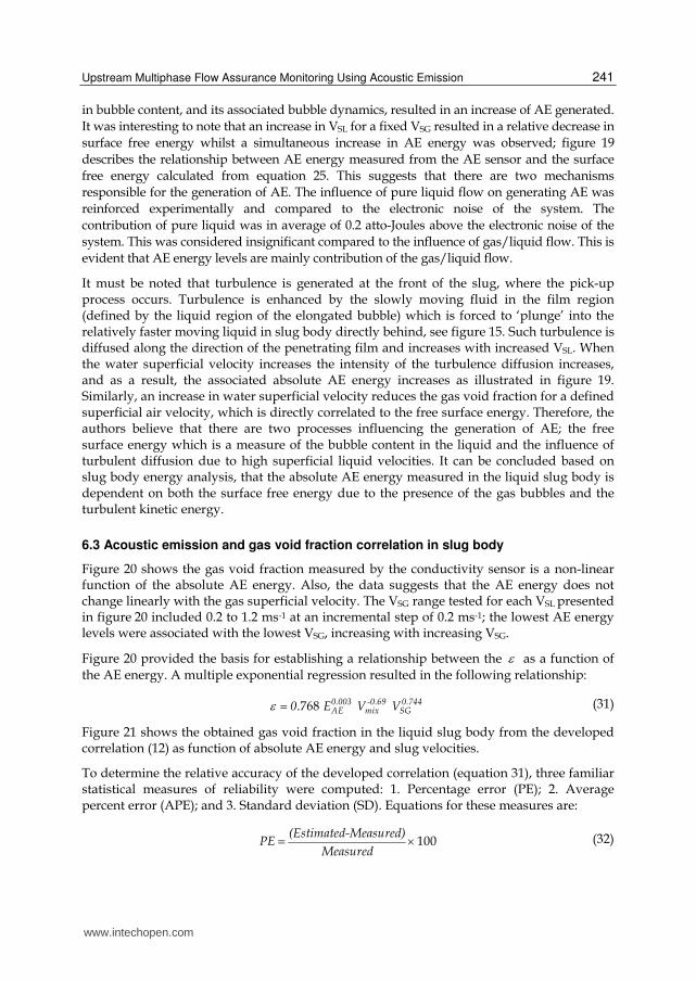
Figure 20 shows the gas void fraction measured by the conductivity sensor is a non-linear function of the absolute AE energy. Also, the data suggests that the AE energy does not change linearly with the gas superficial velocity. The VSG range tested for each VSL presented in figure 20 included 0.2 to 1.2 ms-1 at an incremental step of 0.2 ms-1; the lowest AE energy levels were associated with the lowest VSG, increasing with increasing VSG.

Figure 20 provided the basis for establishing a relationship between the as a function of

the AE energy. A multiple exponential regression resulted in the following relationship:

0.003 -0.69 0.744AE mix SG0 E V V .768 (31)

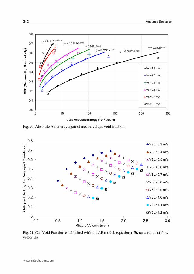
Figure 21 shows the obtained gas void fraction in the liquid slug body from the developed correlation (12) as function of absolute AE energy and slug velocities.

To determine the relative accuracy of the developed correlation (equation 31), three familiar statistical measures of reliability were computed: 1. Percentage error (PE); 2. Average percent error (APE); and 3. Standard deviation (SD). Equations for these measures are:

(Estimated-Measured)PE

Measured100 (32)

www.intechopen.com


Fig. 20. Absolute AE energy against measured gas void fraction

Fig. 21. Gas Void Fraction established with the AE model, equation (15), for a range of flow velocities

www.intechopen.com


n

i 1

PE

APEn

(33)

n n

i ii 1 i 1

2

n (PE PE

SDn

2

2)

(34)

The predictions of the proposed correlation, equation 31, and correlations by several researchers (Gregory at al., 1978; Hughmark, 1962; Ferschneider, 1983) are presented in Table 1. The statistical parameters for the proposed correlation are smaller than those listed in Table 1, demonstrating good performance over all correlations.

APE SD

This study -0.49 3.48

Gregory et al [31] 12.95 10.80

Hughmark [32] 13.90 10.89

Nicklin et al [34] 13.29 14.77

Table 1. Summary of statistical results for correlations

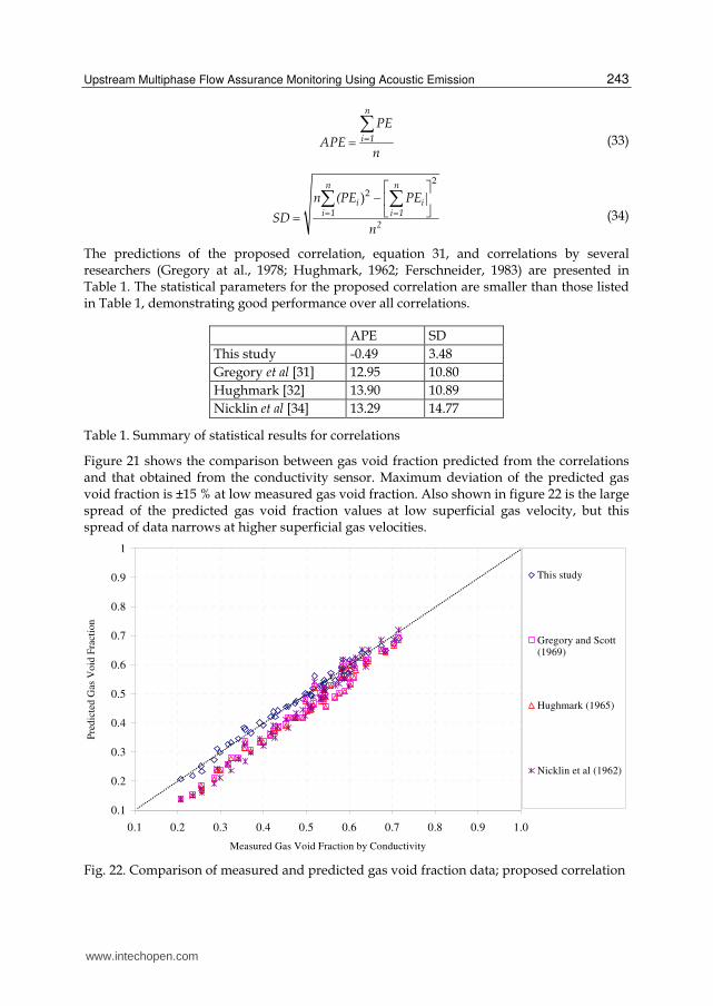
Figure 21 shows the comparison between gas void fraction predicted from the correlations and that obtained from the conductivity sensor. Maximum deviation of the predicted gas void fraction is ±15 % at low measured gas void fraction. Also shown in figure 22 is the large spread of the predicted gas void fraction values at low superficial gas velocity, but this spread of data narrows at higher superficial gas velocities.

Fig. 22. Comparison of measured and predicted gas void fraction data; proposed correlation

0.1

0.2

0.3

0.4

0.5

0.6

0.7

0.8

0.9

1

0.1 0.2 0.3 0.4 0.5 0.6 0.7 0.8 0.9 1.0

Measured Gas Void Fraction by Conductivity

Pre

dic

ted

Gas

Vo

id F

ract

ion

This study

Gregory and Scott(1969)

Hughmark (1965)

Nicklin et al (1962)

www.intechopen.com


One of the main advantage of the proposed correlation is that the AE signals improves with the higher gas fraction, thus increases the accuracy of the prediction even at higher gas fractions. As a result, the proposed correlation can be successfully applied to two-phase air/liquid systems and which have very high percentage of gas void fraction.

7. Conclusions

This work presents preliminary investigations on the application of AE technology for measuring GVF in two-phase air/water under different flow regimes particularly slug flow conditions. It is evident that the main source of Acoustic Emission is directly correlated with the dynamics of bubbles; its formation, coalescence and destruction. Whilst the movement of bubbles in a fluid is known to be associated with oscillations at frequencies of a few kilohertz, it is thought such movement does not generate energy at the frequencies associated with Acoustic Emissions (AE). As defined earlier, the emissions measured in this investigation cover the frequency range of 100kHz to 1,000KHz. The formation and destruction of bubbles is known to be associated with transient pressure pulses which will excite a broad frequency range which will be detectable in the AE frequency range.

The increase of the superficial gas velocities resulted in an increase in AE due to the increase in

bubble content and its associated bubble dynamics. In addition, an increase in the superficial

liquid velocity, result in an increase in the intensity of the turbulence diffusion, also generated

increased AE energy. It has been demonstrated that two mechanisms are responsible for the

generation of AE, the free surface energy which is a measure of the bubble content in the liquid

(air velocity) and the influence of turbulent diffusion (turbulent kinetic energy) due to high

superficial liquid velocities. Furthermore, statistical analysis of the developed correlation

showed the parameters APE and SD to be smaller than the previously reported correlations.

Also, a comparison between the predicted and measured gas void fraction values using

conductivity sensor agree within ±15 %. Finally, the introduction of a new passive and non-

invasive GVF measuring technique utilising AE technology has been proposed for two-phase

air-water flows; providing both a quantitative and qualitative values.

7.1 Recommendations for future work

It has been demonstrated that the time domain analysis of AE signal generated from two-phase gas/water flow is a promising tool in monitoring the flow condition. Although the output identifier parameter adopted in this work was the absolute energy levels of the AE signal, the other parameters such as average signal levels (ASL) and root mean square (RMS) of the AE can also be used to monitor the flow conditions. The successfully developed correlation between the gas void fraction (GVF) and AE generated from the flow need to be more generalised by considering several other parameters such as;

Pipe diameter: Several pipe diameters have to be investigated, and the effect of the pipe diameter needs to be included in the correlation.

Fluid viscosity: Tests to be carried out by using fluids with different viscosity grades.

Pipeline inclination: The current research study covered two-phase flow in the horizontal pipelines. Further work should be performed to include the effect of pipeline inclination using inclined and vertical pipelines, which will add significant knowledge to this research.

www.intechopen.com


Due to the fundamental influence of the bubble content on the generated AE energy, more work has to be done in the frequency domain, in order to investigate the contribution and possibly discriminate the influence of each of the bubble activities such as formation, coalescence and destruction.

8. References

Abouelwafa, M. S. A. and Kendall, E. J. M. (1980). The measurement of component rations in multiphase systems using gamma ray attenuation. Journal of Physics E: Science Instruments. 13, 341-345.

Adamson, A.W., 1990. Physical Chemistry of Surfaces, fifth ed. John Willey and Sons Inc. Addali A., Al-Lababidi S., Mba D. (2007). Application of Acoustic Emission to monitoring

two phase flow, Fourth International Conference on Condition Monitoring, Harrogate, UK

Al-lababidi, S. and Sanderson, M.L., Closure model for two-phase liquid-gas measurement under slug flow conditions. In: Proceedings of the 11th International Conference on Flow Measurement, FLOMEKO’03, Groningen, Netherlands, May 12-14, 2003.

Al-lababidi, S., and Sanderson, M.L. Transit Time Ultrasonic Modelling in Gas/Liquid Intermittent Flow Using Slug Existence Conditions and Void Fraction Analysis”. In: Proceedings of the 12th International Conference on Flow Measurement, FLOMEKO’04, Guilin, China, Sep12-17 2004.

Andreussi, P. and Bendiksen, K. H. (1989). An Investigation of void fraction in liquid slugs for horizontal and inclined gas-liquid pipe flow. International Journal of Multiphase Flow, 15(6), 937-946.

Andreussi, P., Donfrancesco, Di. and Messia, M. (1988). An Impedance Method for the Measurement of Liquid Holdup in Two-Phase Flow. International Journal of Multiphase Flow, 14(6), 777–787.

Barnea, D. and Taitel, Y. (1993). A model for slug length distribution in gas-liquid slug flow. International Journal of Multiphase Flow, 19(5), 829–838.

Barnea, D., Brauner, N., 1985. Holdup of the liquid slug in two-phase intermittent flow. International Journal of Multiphase Flow 11, 43–49.

Beck, M.S., and Plaskowski, A. (1987). Cross-Correlation Flowmeters: Their Design and Application. Bristol, UK: Adam Hilger.

Bendiksen, K. H. (1984). An experimental investigation of the motion of long bubbles in inclined tubes. International Journal of Multiphase Flow, 10(4), 467-483.

Bendiksen, K. H., Malnes, D. and Nydal, O.J. (1996). On the modelling of slug flow. Journal of Chemical Engineering Communications, 141, 71-102.

Bignell, N. and Choi, Y. M. (2001). Volumetric positive-displacement gas flow standard. Journal of Flow Measurement and Instrumentation, 12(4), 245–251.

Boyd, J.W.R. and Varley J. (2001), The uses of passive measurement of acoustic emissions from chemical engineering processes, Chemical Engineering Science, Volume 56, Issue 5, pp1749-1767, ISSN 0009-2509.

Brauner, N., 2001. The prediction of dispersed flow boundaries in liquid–liquid and gas–liquid systems. International Journal of Multiphase Flow 27, 885–910.

Brauner, N., Ullmann, A., 2002. Prediction of holdup in liquid slugs. In: Heat 2002, Third Int. Conf. on Transport Phenomena in Multiphase Flow, IFFM No. 112, pp. 1–15.

www.intechopen.com


Brauner, N., Ullmann, A., 2004. Modelling of gas entrainment from Taylor bubbles. Part B: A stationary bubble. Int. J.Multiphase Flow Vol. 30, pp. 273-290, 2004

Brennen, C. E., (1995) Cavitation Bubble Dynamics, Oxford University Press, ISBN: 0-19-509409-3.

Brill, J. P., Schmidt, Z., Coberly, W. A., Herring, J. D. and Moore. D.W. (1981). Analysis of two-phase tests in large-diameter flow lines Prudhoe Bay Field. SPE Journal, 1981, 363-377.

Brodkey, R.S., 1967. The Phenomena of Fluid Motions. Addisson-Wesley Press. Cheng, W., Murai, Y., Sasaki, T. and Yamamoto, F. (2005). Bubble velocity measurement

with a recursive cross correlation PIV technique. Journal of Flow Measurement and Instrumentation, 16 (1), 35-46.

Corneliussen, S., Couput, J., Dahl, E., Dykesteen, E., Frøysa, K. E., Malde, E., Moestue, H., Moksnes, P. O., Scheers, L. and Tunheim, H. (2005). Handbook of Multiphase Flow. Norwegian Society for Oil and Gas Measurement (NFOGM) and The Norwegian Society of Chartered Technical and Scientific Professionals (Tekna), Norway, Revision 2, March 2005.

Costigan, G. and Whalley, P. B. (1997). Slug Flow Regime Identification From Dynamic Void Fraction Measurement in Vertical Air-Water Flows. International Journal of Multiphase Flow, 23(2), 263-282.

Coull, C. and Sattary, J. (2004). Evaluation of Ultrasonic Technology for Measurement of Multiphase Flow. National Engineering Laboratory, UK, Report No2004/230, November, 2004.

Davies, S. R. (1992). Studies of Two-Phase Intermittent Flow in Pipelines. PhD Thesis, Imperial College, London, UK, 1992.

Derakhshan, O., Houghton, J.R., Jones, R.K. and March, P.A., (1989), Cavitation monitoring of hydroturbines with RMS acoustic emission measurement, Symposium on Acoustic Emission: Current Pratice and Future Directions, Mar 20-23 1989 Published by ASTM, Philadelphia, PA, USA, Charlotte, NC, USA, pp. 305.

Dong, F., Xu, Y. B., Xu, L. J., Hua, L. and Qiao, X. T. (2005). Application of dual-plane ERT system and cross-correlation technique to measure gas-liquid in vertical upward pipe. Journal of Flow Measurement and Instrumentation, 16(2-3), 191-197.

Dukler, A. E. and Hubbard, M. G. (1975). A model for gas-liquid slug flow in horizontal tubes. Industrial and Engineering Chemistry Fundamental. 14 (4), 337-347.

Fan, Z., Lusseyran, F. and Hanratty, T. J. (1993a). Initiation of slugs in horizontal gas-liquid flows. Journal of American Institute of Chemical Engineering . 39, 1741-1753.

Fan, Z., Ruder, Z. and Hanratty, T. J. (1993b). Pressure profiles for slugs in horizontal pipelines. International Journal of Multiphase Flow, 19(3), 421-437.

Ferschneider, G. (1983). Έcoulements Diphasiques Gas-Liquid á Poches et á Bouchon en Conduits. Cited in: Hale, C. P. (2000). Slug Formation, Growth and Decay in Gas-Liquid Flow, chapter 3, p211.PhD Thesis, Imperial College, London, UK, 2000.

Ferschneider, G. (1983). Έcoulements Diphasiques Gas-Liquid á Poches et á Bouchon en Conduits. Cited in: Hale, C. P. (2000). Slug Formation, Growth and Decay in Gas-Liquid Flow, chapter 3, p211.PhD Thesis, Imperial College, London, UK, 2000.

Fossa, M. (1998). Design and Performance of a Conductance Probe for Measuring the Liquid Fraction in Two-Phase Gas-Liquid Flows. Journal of Flow Measurement and Instrumentation, 9, 103-109.

www.intechopen.com


Fossa, M., Guglielmini, G., and Marchitto, A. (2003). Intermittent flow Parameters from Void Fraction Analysis. Journal of Flow Measurement and Instrumentation, 14, 161–168.

Ghassan, H. and Majeed, A. (1999). Liquid slug holdup in horizontal and slightly inclined two-phase slug flow. Journal of Petroleum Science and Engineering 27, 27-32.

Gopal, M. and Jepson, W. P. (1997). Development of digital image analysis techniques for the study of velocity and void profiles in slug flow. International Journal of Multiphase Flow, 23(5), 945-965.

Graham, B; Wallis, G. B. and Dobson, J. E. (1973). The onset of slugging in horizontal stratified air-water flow. International Journal of Multiphase Flow, 1(1), 173-193.

Gregory, G.A. and Scott, D. S. (1969). Correlation of liquid slug velocity and frequency in horizontal cocurrent gas-liquid slug flow. Journal of AIChE, 15, 933-935.

Gregory, G.A., Nicholson, M. and Aziz, K. (1978). Correlation of the liquid volume fraction in the slug for horizontal gas liquid slug flow. International Journal of Multiphase Flow, 4(1), 33–39.

Gregory, G.A., Nicholson, M. and Aziz, K. (1978). Correlation of the liquid volume fraction in the slug for horizontal gas liquid slug flow. International Journal of Multiphase Flow, 4(1), 33–39.

Gurevich, Y. (2001). Performance evaluation and application of clamp-on ultrasonic cross-correlation flow meter CROSSFLOW. In: Proceedings of the International Conference of Flow Measurement, Sao Paolo, Brazil, (date ), 2000.

Hale, C. P. (2000). Slug Formation, Growth and Decay in Gas-Liquid Flow, PhD Thesis, Imperial College, London, UK, 2000.

Hammer, E. A. and Nordtvedt, J. E. (1991). The Application of a Venturi Meter to Multiphase Flow Meters for Oil Well Production. In: Proceedings of the 5th Conference on Sensors and their Applications, London, UK, September 22-25 (Bristol: Adam Hilger).

Hewitt, G. F., Harrison, P. S., Parry, S. J. and Shires, G. L. (1995). Development and Testing of the ‘Mixmeter’ Multiphase Flowmeter. In: Proceedings of the 13th North Sea Flow Measurement Workshop, Lillehammer, Norway, October 24-26 1995.

Hinze, J.O., 1955. Fundamentals of the hydrodynamic mechanism of splitting in dispersion processes. AIChE J. 1, 289.

Hughmark, G. A.,1962 ‘;Holdup in Gas-Liquid Flows,” Chem. Eng.Prog.(April, 1962) 58, 62 Jepson, W. P. and Gopal, M. (1998). Ultrasonic Measuring System and Method of Operation.

U.S Patent, Patent No 5,719,329, (February. 17, 1998). King, M. J. S., Hale, C. P., Roberts, I. F., Fisher, S. A., Lawrence, C. J., Mendes-Tatsis, M. A.

and Hewitt, G. F. (1997). Experimental investigations of flowrate Transients in horizontal pipes. In: Proceedings of the 8th International conference on Multiphase Production, Cannes, France, June 18-20, 1997.

King, N.W. (1990). Subsea multi-Phase Flow Metering a Chanllenge for the Offshore Industry. In: Subsea 90 International Conferences, London, England, December 11-12, 1990.

Kolmogorov, A.N., 1949. On the breaking of drops in turbulent flow. Doklady Akad. Nauk. 66, 825–828.

Kordyban, E. S. (1961). A flow modle for two-phase slug flow in horizontal tubes. Journal of Basic Engineering, TASME, 83, 613-618.

www.intechopen.com


Kordyban, E. S. and Ranov, T. (1970). Mechanism of Slug Formation in Horizontal Two-Phase Flow. Journal of Basic Engineering. 92, 857-864.

Leighton, T. G. (1994). The acoustic bubble, London: Academic Press. Letton, W. (2003). Technique for Measurement of Gas and Liquid Flow Velocities, and

Liquid Holdup in a Pipe with Stratified Flow. U.S Patent, Patent No 6,550,345 B1, (Aprial 22, 2003).

Lunde, O., Asheim, H. (1989). An Experimental Study of Slug Stability in Horizontal Flow. In: Proceedings of the 4th International conference Multiphase Production, Nice, France, June 19-21, 1989.

Malnes, D. (1979). Slip relations and momentum equations in two-phase flow. Cited in: Bendiksen, K. H., Malnes, D. and Nydal, O.J. (1996). On the modelling of slug flow. Journal of Chemical Engineering Communications, 141, 71-102.

Manfield, P. (2000). Experimental, computational and analytical studies of slug flow. PhD Thesis, Imperial College, London, UK, 2000.

Manolis, I. G. (1995). High Pressure Gas-Liquid Slug Flow. PhD Thesis, Imperial College, London, UK, 1995.

Mba, D., Rao, Raj B. K. N.,( 2006) Development of Acoustic Emission Technology for Condition Monitoring and Diagnosis of Rotating Machines: Bearings, Pumps, Gearboxes, Engines, and Rotating Structures. The Shock and Vibration Digest 2006 38: 3-16.

McNulty, P.J. (1985), PUMP HYDRAULIC NOISE: ITS USES AND CURES, Marine Engineers Review, , pp. 22-23.

Mehdizadeh, P. and Williamson, J. (2004). Principles of Multiphase Measurements. Alaska Oil & Gas Conservation Commission, Alaska, USA.

Merilo, M., Dechene, R. L. and Cichowlas, W.M. (1977). Void Fraction Measurement with a Rotating Electric Field Conductance Gauge. ASME Journal of Heat Transfer 99, 330-332.

Miller, R. K. (1987),(Ed.) Acoustic emission testing. ASNT Nondestructive Testing Handbook, 1987, Vol. 5 (American Society of Nondestructive Testing), ISBN: 0-931403-02-2.

Mishima, K. and Ishii, M. (1980). Theoretical prediction of onset of horizontal slug flow. Journal of Fluids Engineering, Transactions of the ASME . 102, 441-445.

Moore, P. I. (2000). Modelling of Installation Effects on Transit Time Ultrasonic Flow Meters in Circular Pipes. PhD Thesis, University of Strathclyde, UK.

Moura, L. F. M. and Marvillet, C. (1997). Measurement of Two-phase Mass Flow Rate and Quality Using Venturi and Void Fraction Meters. In: Proceedings of the 1997 ASME International Mechanical Engineering Congress and Exposition, Dallas, TX, USA, November 16-21, 1997, The Fluids Engineering Division, FED, 1997, Vol. 244, 363-368.

Mwambela, A.J. and Johansen, G.A. (2001). Multiphase flow component volume fraction measurement: experimental evaluation of entropic thresholding methods using an electrical capacitance tomography system. Journal of Measurement Science and Technology, 12, 1092-1101.

Nadler, M. and Mewes, D. (1995). Effect of the viscosity on the phase distribution in horizontal gas-liquid flow. International Journal of Multiphase Flow, 21(2), 253-266.

www.intechopen.com


Nicholson, M. K., Aziz, K. and Gregory, G. A. (1978). Intermittent two-phase phase flow in horizontal pipes: predictive models. The Canadian Journal of Chemical Engineering, 56 (6), 653-663.

Nydal, O.J., Pintus, S. and Andreussi, P. (1992). Statistical characterisation of slug flow in horizontal pipes. International Journal of Multiphase Flow, 18(3), 439-453.

Olsen, A.B. (1993). Framo Subsea Multiphase Flow Meter System Proc.Sem.Multiphase Meters and their Subsea Application, London, England.

Ong, K.H. (1975). Hydraulic Flow Measurement Using Ultrasonic Transducers and Correlation Techniques. PhD thesis. University of Bradford, UK.

Paglianti, A., Andreussi, P.and Nydal, O. J. (1993). The Effect of Fluid Propoerties and Geometry on Void Distribution in Slug Flow. In: Proceedings of the 6th International Conference on Multiphase Production,Cannes, France, June 16-18, 1993.

Pan, L. (1996). High Pressure Three-phase (gas-liquid-liquid) flow. PhD Thesis. Imperial College, London.

Rafa, K., Tomoda, T. and Ridley, R. (1989). Flow Loop Field Testing of a Gamma Ray Compositional Meter. In: Proceedings of the ASME Energy Sources Technology Conference and Exhibition, paper no.89-Pet-7, Houston, Texas, Jan 22-25, 1989.

Reis, E. dos. and Goldstein Jr. L. (2005). A non-intrusive probe for profile and velocity measurement in horizontal slug flows. Journal of Flow Measurement and Instrumentation, 16 (4), 229-239.

Roach, G. J. and Watt, J. S. (1996). Current status development of CSIRO gamma-ray multiphase flow meter. In: Proceedings of the 14th North Sea Flow Measurement Workshop, Peebles, Scotland, October 27-30, 1996.

Ruder, Z., Hanratty, P. H. and Hanratty, T. J. (1989). Necessary conditions for the existence of stable slugs. International Journal of Multiphase Flow, 15(2), 209-226.

Sanderson, M. L. and Yeung, H. (2002). Guidelines for the use of ultrasonic non-invasive metering techniques. Journal of Flow Measurement and Instrumentation, 13: 125–142.

Scott, S. L., Shoham, O. and Brill, J. P. (1986). Prediction of slug length in horizontal large-diameter pipes. In: Proceedings of the 56th Regional Meeting on the Society of Petroleum Engineers, Oakland, CA, April 2-4 (SPE 15103).

Singh, G. and Griffith, P. (1970). Determination of the Pressure Drop Optimum Pipe Size for Two-Phase Slug Flow in an Inclined Pipe. Cited in: Hale, C. P. (2000). Slug Formation, Growth and Decay in Gas-Liquid Flow, chapter 3, p211.PhD Thesis, Imperial College, London, UK, 2000.

Stanislav, J. F. Kokal, S. and Nicholson, M.K. (1986). Intermittent gas-liquid flow in upward inclined pipes. International Journal of Multiphase Flow, 12(3), 33–39.

Steven, R. N. (2002). Wet gas metering with a horizontally mounted Venturi meter. Journal of Flow Measurement and Instrumentation, 12(5-6), 361-372.

Stewart, C. (2001). Instrumentation for the Measurement of Slug Flows. PhD thesis, University of Strathclyde, UK.

Taitel, Y. and Dukler, A. E. (1976). A model for predicting flow regime transitions in horizontal and near horizontal gas-flow. Journal of American Institute of Chemical Engineering. 22(1), 47-55.

Theuveny, B. C., Segeral, G. and Pinguet, B. (2001). Multiphase Flowmeters in Well Testing Applications. In: Proceedings of the SPE Annual Technical Conference and Exhibition, New Orleans, Louisiana, USA, September 30-October 3, 2001, SPE Paper 71475.

www.intechopen.com


Thompson, E. J. (1978). Mid-radius ultrasonic flow measurement FLOMEKO ed H H Dijstelbergen and E A Spencer, pp 153–61.

Thorn, R., Johansen, G. A., and Hammer, E. A. (1997). Recent developments in three phase flow measurement. Measurement Science and Technology, 8(7), 691–701.

Tuss, B., Perry, D. and Shoup, G. (1996). Field tests of the high gas volume fraction multiphase meter. In: Proceedings of the SPE Annual Technical Conference and Exhibition. Denver, USA, October 6-9, 1996, SPE Paper 36594.

Van Santen H., Kolar, Z. I. and Scheers, A.M. (1995). Photo Energy Selection for Dual Energy Gamma and /or X-ray Absorption Composition Measurement in Oil-Water-Gas Mixtures. Journal of Nuclear .Geophysics, 9(3), 193-202.

Vedapuri, D. and Gopal, M. (2003). Determining Gas and Liquid Flow Rates in A Multi-Phase Flow. U.S Patent, Patent No 6,502,465 B1, (January 7, 2003)

Woods, B. D. and Hanratty, T. J. (1996). Relation of Slug Stability to Shedding Rate. International Journal of Multiphase Flow, 22(5), 806-828.

Xie, C. G, Stott, A. L., Plaskowski, A. and Beck, M. S. (1990). Design of capacitance electrodes for concentration measurement of two-phase flow. Journal of Measurement Science and Technology, 1, 65-78.

Xu, L.J., Xu, J., Dong, F. and Zhang, T. (2003). On fluctuation of the dynamic differential pressure signal of Venturi meter for wet gas metering. Journal of Flow Measurement and Instrumentation, 14(4-5), 211-217.

Yang, W. Q. and Beck, M. S. (1997). An intelligent cross correlation for pipelines flow velocity measurement. Journal of Flow Measurement and Instrumentation, 8(2), 77-84.

Zhang, H.J., YUE W.T. and HUANG, Z.Y. (2005). Investigation of Oil-Air Two-Phase Mass Flow rate Measurement using Venturi and Void Fraction Sensor. Journal of Zhejiang University SCIENCE,6A(6),601-606.

Zhang, H.-Q., Wang, Q., Sarica, C., and Brill, J. P., 2003, ‘‘Unified Model for Gas-Liquid Pipe Flow Via Slug Dynamics—Part 2: Model Validation,. ASME J. Energy Resour. Technol., 125,pp.266-273

www.intechopen.com

Acoustic EmissionEdited by Dr. Wojciech Sikorski

ISBN 978-953-51-0056-0Hard cover, 398 pagesPublisher InTechPublished online 02, March, 2012Published in print edition March, 2012

InTech EuropeUniversity Campus STeP Ri Slavka Krautzeka 83/A 51000 Rijeka, Croatia Phone: +385 (51) 770 447 Fax: +385 (51) 686 166www.intechopen.com

InTech ChinaUnit 405, Office Block, Hotel Equatorial Shanghai No.65, Yan An Road (West), Shanghai, 200040, China

Phone: +86-21-62489820 Fax: +86-21-62489821

Acoustic emission (AE) is one of the most important non-destructive testing (NDT) methods for materials,constructions and machines. Acoustic emission is defined as the transient elastic energy that is spontaneouslyreleased when materials undergo deformation, fracture, or both. This interdisciplinary book consists of 17chapters, which widely discuss the most important applications of AE method as machinery and civil structurescondition assessment, fatigue and fracture materials research, detection of material defects and deformations,diagnostics of cutting tools and machine cutting process, monitoring of stress and ageing in materials,research, chemical reactions and phase transitions research, and earthquake prediction.

How to referenceIn order to correctly reference this scholarly work, feel free to copy and paste the following:

Salem Al-Lababidi, David Mba and Abdulmajid Addali (2012). Upstream Multiphase Flow AssuranceMonitoring Using Acoustic Emission, Acoustic Emission, Dr. Wojciech Sikorski (Ed.), ISBN: 978-953-51-0056-0,InTech, Available from: http://www.intechopen.com/books/acoustic-emission/multiphase-flow-assurance-monitoring-using-acoustic-emission

© 2012 The Author(s). Licensee IntechOpen. This is an open access articledistributed under the terms of the Creative Commons Attribution 3.0License, which permits unrestricted use, distribution, and reproduction inany medium, provided the original work is properly cited.

http://creativecommons.org/licenses/by/3.0

upstream multiphase flow assurance monitoring …...upstream multiphase flow assurance monitoring...

Documents