UQ, STAT2201, 2017,Lecture 5

Unit 4 – Joint Distributionsand Unit 5 – Descriptive Statistics.

1

Unit 4 - Joint Probability Distributions

2

A joint probability distribution – two (or more) random variablesin the experiment.

In case of two, referred to as bivariate probability distribution.

3

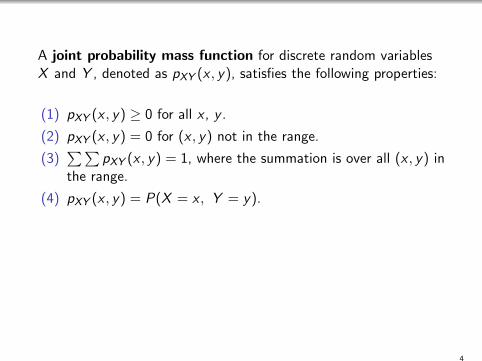
A joint probability mass function for discrete random variablesX and Y , denoted as pXY (x , y), satisfies the following properties:

(1) pXY (x , y) ≥ 0 for all x , y .

(2) pXY (x , y) = 0 for (x , y) not in the range.

(3)∑∑

pXY (x , y) = 1, where the summation is over all (x , y) inthe range.

(4) pXY (x , y) = P(X = x , Y = y).

4

5

Example: Throw two independent dice and look at the,

X ≡ Sum, Y ≡ Product.

6

A joint probability density function for continuous randomvariables X and Y , denoted as fXY (x , y), satisfies the followingproperties:

(1) fXY (x , y) ≥ 0 for all x , y .

(2) fXY (x , y) = 0 for (x , y) not in the range.

(3)∞∫−∞

∞∫−∞

fXY (x , y) dx dy = 1.

(4) For small ∆x , ∆y :

fXY (x , y) ∆x ∆y ≈ P(

(X ,Y ) ∈ [x , x +∆ x)× [y , y +∆ y)).

(5) For any region R of two-dimensional space,

P(

(X ,Y ) ∈ R)

=∫∫R

fXY (x , y) dx dy .

e.g. Height and Weight.

7

8

A joint probability density function can also be defined forn > 2 random variables (as can be a joint probability massfunction). The following needs to hold:

(1) fX1X2...Xn(x1, x2, . . . , xn) ≥ 0.

(2)∞∫−∞

∞∫−∞

. . .∞∫−∞

fX1X2...Xn(x1, x2, . . . , xn)dx1 dx2 . . . dxn = 1.

9

The marginal distributions of X and Y as well as conditionaldistributions of X given a specific value Y = y and vice versa canbe obtained from the joint distribution.

10

If the random variables X and Y are independent, thenfXY (x , y) = fX (x) fY (y) and similarly in the discrete case.

11

Generalized Moments

12

The expected value of a function of two random variables is:

E[h(X ,Y )

]=

∫∫h(x , y)fXY (x , y) dx dy for X ,Y continuous.

13

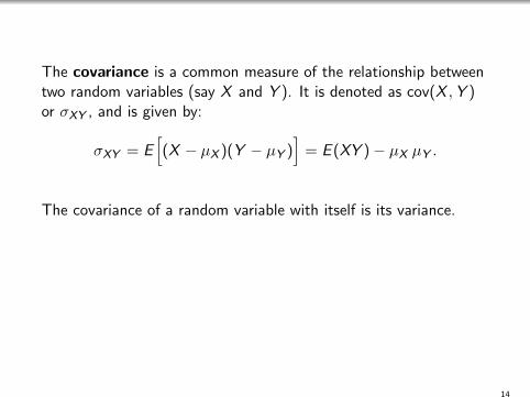
The covariance is a common measure of the relationship betweentwo random variables (say X and Y ). It is denoted as cov(X ,Y )or σXY , and is given by:

σXY = E[(X − µX )(Y − µY )

]= E (XY )− µX µY .

The covariance of a random variable with itself is its variance.

14

The correlation between the random variables X and Y , denotedas ρXY , is

ρXY =cov(X ,Y )√V (X )V (Y )

=σXYσXσY

.

For any two random variables X and Y , −1 ≤ ρXY ≤ 1.

15

If X and Y are independent random variables then σXY = 0 andρXY = 0.

The opposite case does not always hold: In general ρXY = 0 doesnot imply independence.

For jointly Normal random variables it does.

In any case, if ρXY = 0 then the random variables are calleduncorrelated.

16

When considering several random variables, it is common toconsider the (symmetric) Covariance Matrix, Σ withΣi ,j = cov(Xi ,Xj).

17

Bivariate Normal

18

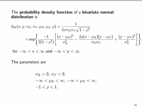
The probability density function of a bivariate normaldistribution is

fXY (x , y ;σX , σY , µX , µY , ρ) =1

2πσXσY√

1− ρ2

× exp

{−1

2(1− ρ2)

[(x − µX )2

σ2X

− 2ρ(x − µX )(y − µY )

σXσY+

(y − µY )2

σ2Y

]}

for −∞ < x <∞ and −∞ < y <∞.

The parameters are

σX > 0, σY > 0,

−∞ < µX <∞, −∞ < µY <∞,

−1 < ρ < 1.

19

20

Linear Combinations of Random Variables

21

Given random variables X1,X2, . . . ,Xn and constants c1, c2, . . . , cn,the (scalar) linear combination

Y = c1X1 + c2X2 + · · ·+ cnXn

is often a random variable of interest.

22

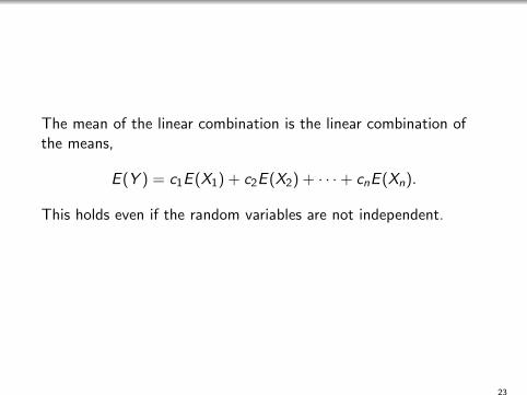
The mean of the linear combination is the linear combination ofthe means,

E (Y ) = c1E (X1) + c2E (X2) + · · ·+ cnE (Xn).

This holds even if the random variables are not independent.

23

The variance of the linear combination is as follows:

V (Y ) = c21V (X1)+c22V (X2)+· · ·+c2nV (Xn)+2∑i<j

∑cicjcov(Xi ,Xj)

24

If X1,X2, . . . ,Xn are independent (or even if they are justuncorrelated).

V (Y ) = c21V (X1) + c22V (X2) + · · ·+ c2nV (Xn).

25

Example: Derive Mean and variance of the Binomial Distribution.

26

Linear Combinations of Normal Random Variables

27

Linear combinations of Normal random variables remainNormally distributed:

If X1, . . . ,Xn are jointly Normal then,

Y ∼ Normal(E (Y ),V (Y )

).

28

i.i.d. Random Samples

29

A collection of random variables, X1, . . . ,Xn is said to be i.i.d., orindependent and identically distributed if they are mutuallyindependent and identically distributed.

The (n - dimensional) joint probability density is a product of theindividual densities.

30

In the context of statistics, a random sample is often modelled asan i.i.d. vector of random variables. X1, . . . ,Xn.

An important linear combination associated with a random sampleis the sample mean:

X =

∑ni=1 Xi

n=

1

nX1 +

1

nX2 + . . .+

1

nXn.

31

If Xi has mean µ and variance σ2 then sample mean (of an i.i.d.sample) has,

E (X ) = µ, V (X ) =σ2

n.

32

Unit 5 – Descriptive Statistics

33

Descriptive statistics deals with summarizing data usingnumbers, qualitative summaries, tables and graphs.

There are many possible data configurations...

34

Single sample: x1, x2, . . . , xn.

35

Single sample over time (time series): xt1 , xt2 , . . . , xtn witht1 < t2 < . . . < tn.

36

Two samples: x1, . . . , xn and y1, . . . , ym.

37

Generalizations from two samples to k samples (each of potentiallydifferent sample size, n1, . . . , nk).

38

Observations in tuples: (x1, y1), (x2, y2), . . . , (xn, yn).

39

Generalizations from tuples to vector observations (each vector oflength `),

(x11 , . . . , x`1), . . . , (x1n , . . . , x

`n).

40

Individual variables may be categorical or numerical.

Categorical variables may be ordinal meaning that they be sorted(e.g. “a”, “b”, “c”, “d”), or not ordinal (e.g. “cat”, “dog”,“fish”).

41

A Statistic

42

A statistic is a quantity computed from a sample (assume here asingle sample x1, . . . , xn).

43

The sample mean: x =x1 + · · ·+ xn

n=

n∑i=1

xi

n.

44

The sample variance: s2 =

n∑i=1

(xi − x)2

n − 1=

n∑i=1

x2i − n x2

n − 1.

The sample standard deviation: s =√s2.

45

Order Statistics

46

Order statistics: Sort the sample to obtain the sequence of sortedobservations, denoted x(1), . . . , x(n) where, x(1) ≤ x(2) ≤ . . . ≤ x(n).

Some common order statistics:

The minimum min(x1, . . . , xn) = x(1).

The maximum max(x1, . . . , xn) = x(n).

The median

median =

{x( n+1

2) if n is odd,

12

(x( n

2) + x( n

2+1)

)if n is even.

The median is the 50’th percentile and the 2ndquartile (see below).

47

The q th quantile (q ∈ [0, 1]) or alternatively thep = 100q percentile (measured in percents insteadof a decimal), is the observation such that p percentof the observations are less than it and (1− p)percent of the observations are greater than it.

The first quartile, denoted Q1 is the 25th percentile.The second quartile (Q2) is the median. The thirdquartile, denoted Q3 is the 75th percentile. Thushalf of the observations lie between Q1 and Q3. Inother words, the quartiles break the sample into 4quarters. The difference Q3− Q1 is theinterquartile range.

The sample range is x(n) − x(1).

48

Interlude: The quantile of a probability distribution?

Given α ∈ [0, 1] : What is x such that P(X ≤ x) = α,

F (x) = α.

Or, ∫ x

−∞u du = α.

To find the quantile, solve the equation for x .

49

Visualization

50

Histogram (with Equal Bin Widths):

(1) Label the bin (class interval) boundaries on a horizontal scale.

(2) Mark and label the vertical scale with frequencies or counts.

(3) Above each bin, draw a rectangle where height is equal to thefrequency (or count).

51

A Kernel Density Estimate (KDE) is a way to construct aSmoothed Histogram.

While construction is not as straightforward as steps (1)–(3)above, automated tools can be used.

52

Both the histogram and the KDE are not unique in the way theysummarize data.

With these methods, different settings (e.g. number of bins inhistograms or bandwidth in a KDE) may yield differentrepresentations of the same data set.

Nevertheless, they are both very common, sensible and usefulvisualisations of data.

53

The box plot is a graphical display that simultaneously describesseveral important features of a data set:

Centre.

Spread.

Departure from symmetry.

Identification of unusual observations or outliers.

It is often common to plot several box plots next to each other forcomparison.

54

55

An anachronistic, but useful way for summarising small data-sets isthe stem and leaf diagram.

56

In a cumulative frequency plot the height of each bar is the totalnumber of observations that are less than or equal to the upperlimit of the bin.

57

The Empirical Cumulative Distribution Function (ECDF) is,

F̂ (x) =1

n

n∑i=1

1{xi ≤ x}.

Here 1{·} is the indicator function. The ECDF is a function ofthe data, defined for all x .

58

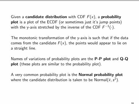
Given a candidate distribution with CDF F (x), a probabilityplot is a plot of the ECDF (or sometimes just it’s jump points)with the y-axis stretched by the inverse of the CDF F−1(·).

The monotonic transformation of the y-axis is such that if the datacomes from the candidate F (x), the points would appear to lie ona straight line.

Names of variations of probability plots are the P-P plot and Q-Qplot (these plots are similar to the probability plot).

A very common probability plot is the Normal probability plotwhere the candidate distribution is taken to be Normal(x , s2).

59

The Normal probability plot can be useful in identifyingdistributions that are symmetric but that have tails that are“heavier” or “lighter” than the Normal.

60

A time series plot is a graph in which the vertical axis denotes theobserved value of the variable and the horizontal axis denotes time.

61

A scatter diagram is constructed by plotting each pair ofobservations with one measurement in the pair on the vertical axisof the graph and the other measurement in the pair on thehorizontal axis.

62

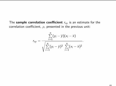
The sample correlation coefficient rxy is an estimate for thecorrelation coefficient, ρ, presented in the previous unit:

rxy =

n∑i=1

(yi − y)(xi − x)√n∑

i=1(yi − y)2

n∑i=1

(xi − x)2

.

63