urban energy information modeling – a framework for ... · integrate the effect of the...

URBAN ENERGY INFORMATION MODELING – A FRAMEWORK FOR COUPLING MACRO-MICRO FACTORS AFFECTING BUILDING ENERGY

CONSUMPTION Shalini Ramesh1, Khee Poh Lam1

1Center for Building Performance and Diagnostics Carnegie Mellon University, Pittsburgh, PA, USA

ABSTRACT Residential and commercial buildings in the U.S. consume 47.6% of the total energy (Architecture 2030). The atmospheric interactions and energy fluxes between the natural and built environment influence the urban climate causing urban heat islands on the macro scale and impacts building energy consumption on the micro scale. Therefore, it is important to integrate the effect of the macro-micro factors to reduce building energy consumption. Firstly, this paper evaluates the accuracy between measured and simulated microclimate and its effect on building cooling load using a case study located in Pittsburgh, Pennsylvania, USA. Results show, the average hourly deviation between measured and simulated air temperature is 8.25% and relative humidity is 10.05%. Secondly, a coupling framework is proposed for ENVI-met 4.0 (microclimate simulation tool) and EnergyPlus (whole - building energy simulation tool) using Building Controls Virtual Test Bed (BCVTB) as the coupling platform.

INTRODUCTION Land use changes due to urbanization is causing higher temperatures in the urban areas compared to the sub-urban areas. This phenomenon known as urban heat island (UHI) is an extreme case of how land use modifies the regional and the microclimate. The external factors at the macro level influencing the urban microclimate are reduced vegetation cover, impervious surface area, anthropogenic heat and air pollutants. Internal factors at the micro level relate to building morphology in cityscapes, building systems and enclosures. These macro and micro level factors together are a major cause of urban heat island. UHI not only affects the urban climatic conditions but also affects building heating and cooling loads to a great extent. A UHI study in Athens, Greece between 1970-2010 showed a cooling load increase of 28.6% and decrease in heating load by 19.5% (Kapsomenakis, 2013). A study in Washington, USA between 1960-2000 showed a temporal variability of the heating and cooling load of 9.2% (Crawley, 2008). The study was based on the increase/decrease of heating and cooling degree days. Several other studies validating the increase in cooling load and decrease in heating load for cooling dominated climates have been documented by (Santamouris, 2014)

All these studies also demonstrate that measures adopted to reduce UHI can reduce summer cooling loads based on the location and climatic conditions. Although UHI mitigation helps in reduction of cooling loads, few studies have shown that increased urban temperatures in heating dominated climates can reduce heating loads during the winter season. Though increase in UHI can be beneficial for buildings in heating dominated climates in terms of conserving heating energy, it can be detrimental to the local microclimate in terms of destruction of natural habitat, climate change with severe winter or summer temperatures. Therefore, necessary measures have to be implemented to reduce UHI at the macro scale and its effects on building energy consumption at the micro scale. The thermal performance of a building and its energy consumption are directly affected by the building internal loads, its inside and outside conditions as well as the energy fluxes with the surrounding environment. Simulating the microclimate can be achieved using various methods like: (1) data-driven models e.g., artificial neural network model mainly to predict UHI intensity (2) deriving weather data from LIDAR imagery using tools e.g., ERDAS (3)softwares like CitySim and Urban Modeling Interface (UMI). Likewise, simulation tools like Green Building Studio, eQUEST, IES +VE, and EnergyPlus are able to simulate whole building energy consumption right from the conceptual design phase through the building life-cycle. However, the methods listed above to simulate the microclimate do not take into consideration all microclimate factors such as buildings, vegetation, water bodies, natural surfaces, soils, pollution particles (Yang, 2012). In addition, they do not provide adequate model resolution from the macro to the micro level to calculate the boundary conditions of all the surfaces with respect to the microclimate. This research differentiates itself by providing a coupling framework for the two most sophisticated macro and micro level simulation tools, ENVI-met and EnergyPlus. The research uses ENVI-met v4.0, which takes in to account all the above described requirements while providing macro to micro level building resolution to simulate the local microclimate. EnergyPlus is used to simulate the whole building energy consumption using the weather file simulated by ENVI-met. Based on (Yang, 2012), and assessing the accuracy of the simulated and measured data, a

Proceedings of BS2015: 14th Conference of International Building Performance Simulation Association, Hyderabad, India, Dec. 7-9, 2015.

- 601 -

coupling framework is proposed for the CSL case study using BCVTB.

OBJECTIVES The objectives of this study are: 1. Compare the accuracy of the simulated

microclimate parameters: air temperature, relative humidity, wind speed with measured data from the weather station located on the case study site.

2. Discuss a framework for enhancing and testing the stability of the coupling platform for macro (ENVI-met) and micro level factors (EnergyPlus) using the coupling tool, BCVTB.

METHOD 1.1. Introduction of microclimate simulation tool

– ENVI-met ENVI-met v4.0 is a prognostic three-dimensional climate simulation tool that adheres to all the above-mentioned requirements and hence is used in this case study to measure the accuracy of simulated and measured microclimate data. ENVI-met simulation is based on spatial as well as temporal model resolutions, i.e., it can simulate between 0.5m-10m per grid resolution spatially with time steps ≤ 10s. The model structure consists of three main components: • 1D boundary model: Used for initialization of

boundary conditions to be used by the 3D atmospheric model.

• 3D atmospheric model: Simulation of buildings, vegetation and digital elevation model.

• 3D/1D soil model: Calculate temperature and humidity fluxes within the soil.

Four important criteria required to accurately simulate the physics of the atmospheric boundary layer are: A. The grid resolution of the model area should be

≤10m to provide building level accuracy B. The energy balance of all surfaces types should

be implemented C. The implementation of simulation of plants

both in terms of physical and physiological properties

D. A prognostic and transient model is required for the calculation of the atmospheric processes.

The model is capable of simulating airflow around and between buildings, heat and moisture exchange processes at all surfaces, turbulence, exchange of energy and mass between vegetation and its surroundings and gas and particle dispersion (Yang, 2012).

1.2 Case study description The case study selected for this study is a zero-energy LEED Platinum certified medium-size office building – Phipps Center for Sustainable Landscapes (CSL) in Pittsburgh, Pennsylvania, USA as shown in Figure 1. The building is a 2,262

m2 education, research and administration facility. The site location is considered as an urban area due to higher air temperatures compared to the AMY (Actual Meteorological Year) site located in a sub-urban area.

Figure 1 Aerial image of the CSL case study area and its

surroundings The case study is strategically selected keeping in mind three important criteria’s: 1. The area has various land uses such as office

building, naturally ventilated botanical garden (Phipps Conservatory), vegetated areas (Schenley Park) and a lake, northeast of the CSL building.

2. The CSL building is adjacent to Carnegie Mellon University campus, which has a dense network of administrative, educational, resident halls and parking lots. This provides potential for expanding the study area to evaluate the influence of built environment on the urban microclimate and vice versa in terms of energy consumption.

3. The CSL building has on-site weather station, that helps in comparison of simulated data with actual on-site data rather than a local weather station near the airport (suburban).

4. The CSL building also has a calibrated EnergyPlus whole building energy model. This helps in accurate estimation and comparison of heating/cooling loads from simulation and measured data using the BCVTB coupling framework.

1.3 Simulation Input Parameters Figure 2 shows the plan and 3D view of the CSL case study area built using ENVI-met v4.0 and the EnergyPlus model. A domain size of 80 m × 80 m × 30 m with a 5 m grid is used for the model area. Table 1 highlights the initial model setup input parameters, which is used to model the CSL case study area. Table 1 ENVI-met model setup input parameters

Model input parameter Input Domain size 80 m × 80 m × 30 m Grid size 5 m Location 40.44° N,-79.98° W Reference time-zone UTC -5:00 Weather data On-site weather station Simulation period July 24 – 27, 2014


- 602 -

Figure 2 2D and 3D view of the CSL case study area as modelled in ENVI-met v4.0 and EnergyPlus

As seen in Figure 3, the air temperature and relative humidity follow a steady profile on July 24 whereas on July 25, there is a decrease (4.5°C) and increase (3°C) in air temperature between 5am - 6am and 2pm - 6pm, in comparison to the profile of July 24. Therefore, by understanding the pattern of initialization inputs, it is possible to initialize the model representing the air temperature and relative humidity pattern for the whole simulation period. By doing so, it is possible to obtain results that is comparable to the measured data. Figure 4 shows the comparison in air temperature and relative humidity between the on-site measured and the remote AMY weather station. There is a clear indication of increased air temperature in the urban

areas compared to the sub-urban areas indicating the presence of urban heat island effect in Pittsburgh, PA. Figure 5 shows the input parameters for the two input components in ENVI-met: area input file and configuration file. The figure provides details on the information source for each of the input parameters. Once the 3D model is setup based on the area input file, the model is initialized using the configuration input file in ENVI-met. The simulation period selected is July 24-27, 2014 which is a peak summer period in Pittsburgh, USA based on temperature profile. In order to understand the effect of initializing the ENVI-met simulation accurately, two 24-hour periods between 7/24/2014 – 7/25/2014 are selected as initialization inputs.

Figure 3 Initialization periods used for case 01 and case 02 of the simulation

Figure 4 Comparison of air temperature and relative humidity of on-site and AMY weather file

20.00

30.00

40.00

50.00

60.00

70.00

80.00

90.00

10.00

13.00

16.00

19.00

22.00

25.00

28.00

24 2 4 6 8 10 12 14 16 18 20 22 24 2 4 6 8 10 12 14 16 18 20 22 24

Rel

ativ

e Hum

idity

(%)

Air

Tem

pera

ture

(°C

)

Hour of Day (07/24/2014-07/25/2014)Temperature Relative Humidity

Initialization - Case 02 (July 24) Initialization - Case 01 (July 25)

20.00

30.00

40.00

50.00

60.00

70.00

80.00

90.00

10.00

13.00

16.00

19.00

22.00

25.00

28.00

7 9 11 13 15 17 19 21 23 1 3 5 7 9 11 13 15 17 19 21 23 1 3 5 7Hour of day (7/24/2014 - 7/26/2014)

Rel

ativ

e Hum

idity

(%)

Air

Tem

pera

ture

(°C

)

T measured T AMY RH measured RH AMY

July 24 July 25 July 26


- 603 -

Configuration input file

Area input file

Macro level Input parameters into ENVI-met

Micro level Input parameters into ENVI-met

Initial meteorological conditions- Wind speed measured in 10m height(m/s)- Wind direction (degrees)- Roughness length at measurement site- Initial atmospheric temperature1 (K)- Specific humidity at model top (g/kg)- Relative humidity1 (%)Solar radiation adjustment factorCloud coverTurbulence model- Turbulence closure scheme for 1D reference model- Upper boundary conditions for TKE and dissipation rate for 3D modelLateral boundary conditions- Temperature and humidity- TurbulenceModel Timing- Dynamic time step managementSoil and Plants- Soil layer wetness - Soil layer temperature- Plant model

On-site Weather Station

ENVI-met Simulation Tool Default Assumption

CSL Calibrated Energy Plus Model

Model Domain- x-grids, y-grids, z-grids- Size of grid cellWall/Roof Properties2

Geographic properties- Location on earth- Latitude, Longitude- Reference time zoneModel rotation out of grid northBuilding geometrySurrounding geometryDigital elevation modelVegetationReceptors3

Soil and natural surfaces

Google Earth Imagery

Scale of Model Input Parameters

Model Input Parameters

Source of Model Input Parameters

User Input

Figure 5 Flowchart indicating macro-micro ENVI-met simulation input parameters and information source

1. Forcing meteorology inputs: By forcing air temperature and relative humidity for a 24-hour period, the tool allows the user to manually define the diurnal variations at the inflow boundary conditions. This feature allows a realistic comparison of simulated and measured data in ENVI-met v4.0. The 24-hour forcing is a representation of the air temperature and relative humidity of the whole simulation period. At the start and during a simulation, ENVI-met checks the current step of the simulation and the forcing input, interpolates the values temporally and spatially. This value is used in the 1D-profile inflow boundary conditions. A linear interpolation is performed for the air temperature and relative humidity forcing inputs (Huttner, 2012).

2. Wall/Roof properties: Specify wall and roof properties based on the construction layers and properties of the individual construction layers. ENVI-met v4.0 is capable of modelling construction materials for up to three layers from the outside to the inside of the wall/roof.

3. Receptors: Selected points inside the model, which provide results on the state of the atmosphere, the surface and the soil at each of these selected points.


- 604 -

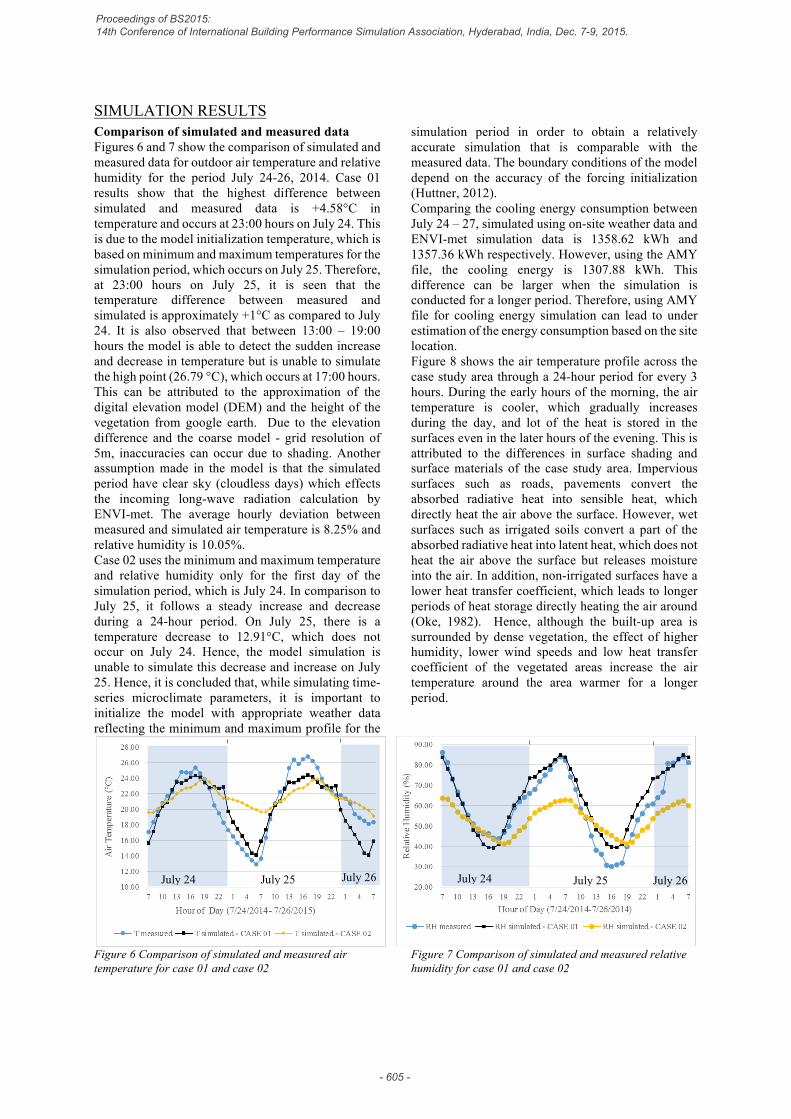
SIMULATION RESULTSComparison of simulated and measured data Figures 6 and 7 show the comparison of simulated and measured data for outdoor air temperature and relative humidity for the period July 24-26, 2014. Case 01 results show that the highest difference between simulated and measured data is +4.58°C in temperature and occurs at 23:00 hours on July 24. This is due to the model initialization temperature, which is based on minimum and maximum temperatures for the simulation period, which occurs on July 25. Therefore, at 23:00 hours on July 25, it is seen that the temperature difference between measured and simulated is approximately +1°C as compared to July 24. It is also observed that between 13:00 – 19:00 hours the model is able to detect the sudden increase and decrease in temperature but is unable to simulate the high point (26.79 °C), which occurs at 17:00 hours. This can be attributed to the approximation of the digital elevation model (DEM) and the height of the vegetation from google earth. Due to the elevation difference and the coarse model - grid resolution of 5m, inaccuracies can occur due to shading. Another assumption made in the model is that the simulated period have clear sky (cloudless days) which effects the incoming long-wave radiation calculation by ENVI-met. The average hourly deviation between measured and simulated air temperature is 8.25% and relative humidity is 10.05%. Case 02 uses the minimum and maximum temperature and relative humidity only for the first day of the simulation period, which is July 24. In comparison to July 25, it follows a steady increase and decrease during a 24-hour period. On July 25, there is a temperature decrease to 12.91°C, which does not occur on July 24. Hence, the model simulation is unable to simulate this decrease and increase on July 25. Hence, it is concluded that, while simulating time-series microclimate parameters, it is important to initialize the model with appropriate weather data reflecting the minimum and maximum profile for the

simulation period in order to obtain a relatively accurate simulation that is comparable with the measured data. The boundary conditions of the model depend on the accuracy of the forcing initialization (Huttner, 2012). Comparing the cooling energy consumption between July 24 – 27, simulated using on-site weather data and ENVI-met simulation data is 1358.62 kWh and 1357.36 kWh respectively. However, using the AMY file, the cooling energy is 1307.88 kWh. This difference can be larger when the simulation is conducted for a longer period. Therefore, using AMY file for cooling energy simulation can lead to under estimation of the energy consumption based on the site location. Figure 8 shows the air temperature profile across the case study area through a 24-hour period for every 3 hours. During the early hours of the morning, the air temperature is cooler, which gradually increases during the day, and lot of the heat is stored in the surfaces even in the later hours of the evening. This is attributed to the differences in surface shading and surface materials of the case study area. Impervious surfaces such as roads, pavements convert the absorbed radiative heat into sensible heat, which directly heat the air above the surface. However, wet surfaces such as irrigated soils convert a part of the absorbed radiative heat into latent heat, which does not heat the air above the surface but releases moisture into the air. In addition, non-irrigated surfaces have a lower heat transfer coefficient, which leads to longer periods of heat storage directly heating the air around (Oke, 1982). Hence, although the built-up area is surrounded by dense vegetation, the effect of higher humidity, lower wind speeds and low heat transfer coefficient of the vegetated areas increase the air temperature around the area warmer for a longer period.

Figure 6 Comparison of simulated and measured air temperature for case 01 and case 02

Figure 7 Comparison of simulated and measured relative humidity for case 01 and case 02

July 24 July 25 July 26 July 24 July 25 July 26


- 605 -

Figure 8 Air temperature profile for July 24 – 25, 2014 across the CSL case study area

COUPLING FRAMEWORK Figure 10 provides the framework for the ENVI-met – EnergyPlus coupling using BCVTB. The coupling process is a two-step process. The first step is to replace the microclimate variables such as air temperature, specific and relative humidity, wind speed and wind direction in the .epw weather file with the calculated average values. The second step is to over-write the calculated combined outside face convection heat transfer coefficient (CHTC) in EnergyPlus. In EnergyPlus, the building surfaces are specified as single entities using geometric coordinates as well as referenced constructions. However, in ENVI-met, grids and meshes are used for defining the building geometry as shown in Figure 9. The ENVI-met input file is setup with receptors along the building façade, which records the microclimate conditions at every grid cell. The average value for each of the receptor output variable is calculated for the corresponding façade based on the façade height in the receptor output file. This overwriting of convection heat transfer coefficient for the respective facades is done using the object, SurfaceProperty:OtherSideCoefficients. The variables required for this calculation is detailed in Table 2. Using these variables, based on the CHTC values in the current time-step, the temperature of the outside air or the exterior surface is calculated. This calculated temperature of the outside air or the exterior surface over-writes the value in the simulation in the next time-step. The following equation shows the calculation of air temperature/surface temperature according to the EnergyPlus calculated CHTC. The air

temperature/surface temperature is obtained from ENVI-met simulation output files. 𝑇 = 𝐶2 ∗ 𝐶3 + 𝐶4 ∗ 𝑇𝑜𝑎𝑑𝑏 + 𝐶5 ∗ 𝑇𝑔𝑟𝑛𝑑 + 𝐶6 ∗𝑊𝑠𝑝𝑑 + 𝐶7 ∗ 𝑇𝑧𝑜𝑛𝑒 + 𝐶8 ∗ 𝑇𝑝𝑎𝑠𝑡 T = Outside air temperature when CHTC >0 W/m2K T = Exterior surface temperature when CHTC <=0 W/m2K Tzone = Temperature of the zone being simulated (°C) Toadb = Dry-bulb temperature of the outdoor air (°C) Tgrnd = Temperature of the ground (°C) Wspd = Outdoor wind speed (m/sec) Tpast = Other side temperature from previous zone timestep (°C)

Figure 9 ENVI-met geometry structure used for coupling


- 606 -

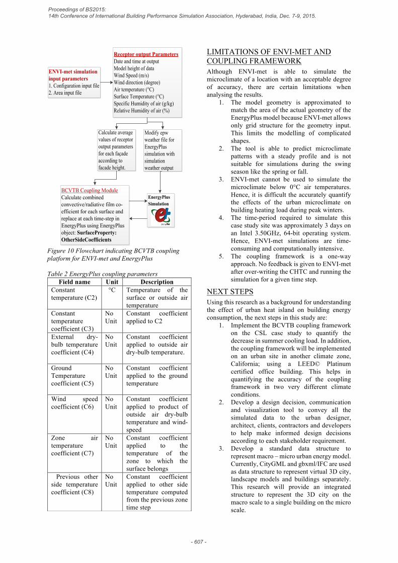
Figure 10 Flowchart indicating BCVTB coupling platform for ENVI-met and EnergyPlus Table 2 EnergyPlus coupling parameters

LIMITATIONS OF ENVI-MET AND COUPLING FRAMEWORK Although ENVI-met is able to simulate the microclimate of a location with an acceptable degree of accuracy, there are certain limitations when analysing the results.

1. The model geometry is approximated to match the area of the actual geometry of the EnergyPlus model because ENVI-met allows only grid structure for the geometry input. This limits the modelling of complicated shapes.

2. The tool is able to predict microclimate patterns with a steady profile and is not suitable for simulations during the swing season like the spring or fall.

3. ENVI-met cannot be used to simulate the microclimate below 0°C air temperatures. Hence, it is difficult the accurately quantify the effects of the urban microclimate on building heating load during peak winters.

4. The time-period required to simulate this case study site was approximately 3 days on an Intel 3.50GHz, 64-bit operating system. Hence, ENVI-met simulations are time-consuming and computationally intensive.

5. The coupling framework is a one-way approach. No feedback is given to ENVI-met after over-writing the CHTC and running the simulation for a given time step.

NEXT STEPS Using this research as a background for understanding the effect of urban heat island on building energy consumption, the next steps in this study are:

1. Implement the BCVTB coupling framework on the CSL case study to quantify the decrease in summer cooling load. In addition, the coupling framework will be implemented on an urban site in another climate zone, California; using a LEED© Platinum certified office building. This helps in quantifying the accuracy of the coupling framework in two very different climate conditions.

2. Develop a design decision, communication and visualization tool to convey all the simulated data to the urban designer, architect, clients, contractors and developers to help make informed design decisions according to each stakeholder requirement.

3. Develop a standard data structure to represent macro – micro urban energy model. Currently, CityGML and gbxml/IFC are used as data structure to represent virtual 3D city, landscape models and buildings separately. This research will provide an integrated structure to represent the 3D city on the macro scale to a single building on the micro scale.

Calculate average values of receptor output parameters for each façade according to facade height.

Modify epw weather file for EnergyPlus simulation with simulation weather output

Receptor output ParametersDate and time at outputModel height of dataWind Speed (m/s)Wind direction (degree)Air temperature (°C)Surface Temperature (°C)Specific Humidity of air (g/kg)Relative Humidity of air (%)

BCVTB Coupling Module Calculate combined convective/radiative film co-efficient for each surface and replace at each time-step in EnergyPlus using EnergyPlus object: SurfaceProperty:OtherSideCoefficients

ENVI-met simulation input parameters1. Configuration input file2. Area input file

EnergyPlus Simulation

Field name Unit Description Constant temperature (C2)

°C Temperature of the surface or outside air temperature

Constant temperature coefficient (C3)

No Unit

Constant coefficient applied to C2

External dry-bulb temperature coefficient (C4)

No Unit

Constant coefficient applied to outside air dry-bulb temperature.

Ground Temperature coefficient (C5)

No Unit

Constant coefficient applied to the ground temperature

Wind speed coefficient (C6)

No Unit

Constant coefficient applied to product of outside air dry-bulb temperature and wind-speed

Zone air temperature coefficient (C7)

No Unit

Constant coefficient applied to the temperature of the zone to which the surface belongs

Previous other side temperature coefficient (C8)

No Unit

Constant coefficient applied to other side temperature computed from the previous zone time step


- 607 -

CONCLUSION This paper has shown the process of modelling an urban area surrounded by various land uses using ENVI-met v4.0 employing the concept of forcing in order to compare the accuracy of simulated and measured microclimate parameters. The paper also proposes a coupling framework for ENVI-met and EnergyPlus, which can be used to evaluate the effect of the microclimate on building energy consumption. This can be effectively used by the design team to evaluate measures for reducing building energy consumption. Although ENVI-met – EnergyPlus coupling has certain limitations, some of the major findings are:

1. The cooling load for the simulation period between July 24 - July 27 is reduced by 4% when using the simulated weather file representing the site conditions as compared to the remote AMY weather file. Therefore, it is important to integrate the effect of UHI on a macro – micro level and quantify its effects not only on the microclimate but also on building energy consumption.

2. The comparison of simulated and measured data clearly indicates that the accuracy of the simulation results depend on the accuracy of the initialization inputs. Using the concept of forcing 24 hours of temperature and relative humidity, it is possible to simulate the actual microclimate of the urban area.

3. The comparison of AMY weather file and measured data shows that it is important to have a measurement point close to the case study site rather than a sub-urban weather station in order achieve simulation results representing the site microclimate accurately.

4. There are certain times were the simulation is unable to meet the increase and decrease in temperature even with accurate forcing of boundary conditions. This is attributed to the cubic grid structure of the model and the relatively course grid (5m x 5m) of the model area which causes inaccuracies in shading calculations. Another reason is due to the approximation of the digital elevation model and vegetation from google earth. As a next step to improve the accuracy of the DEM, LIDAR data can be converted using ArcGIS to create the DEM files that can be used in ENVI-met.

5. With the simulated results, it is possible to develop the coupling platform between ENVI-met and EnergyPlus, which helps in integrating the macro-micro environmental and building conditions to study the effect of the urban microclimate on building energy consumption through direct simulation.

REFERENCES 2030, A. (n.d.). Why buildings? Retrieved from Architecture

2030: http://architecture2030.org/buildings_problem_why/

Bruse, M. (2008). Visualisation of ENVI-met Model Results using LEONARDO 3.X.

Bruse, M. (2015, April). ENVI-met 3.1 Manual Contents. Retrieved from http://www.envi-met.info/documents/onlinehelpv3/helpindex.htm

Bruse, M. (2015, April). The Hitchhiker's Guide to ENVI-met. Retrieved from ENVI-met Board: http://www.model.envi-met.com/hg2e/doku.php?id=forum:start

Crawley, D. B. (2008). Estimating the impacts of climate change and urbanization on building performance. Journal of Building Performance Simulation, 91--115.

Dorer, V. a. (2013). Modelling the urban microclimate and its impact on the energy demand of buildings and building clusters. Proceedings of Building Simulation 2013 (pp. 3483-3489). Chambery, France: International Building Performance Simulation Association (IBPSA).

Evins, R. a. (2014). Simulating external longwave radiation exchange for buildings. Energy and Buildings, 472-482.

Huttner, S. (2012). Further development and application of the 3Dmicroclimate simulation ENVI-met. Mainz: University of Mainz.

Kapsomenakis, J. a. (2013). Forty years increase of the air ambient temperature in Greece: the impact on buildings. Energy Conversion and Management, 353-365.

Kolokotroni, M. a. (2007). The London Heat Island and building cooling design. Solar Energy, 102-110.

Kolokotroni, M. a. (2011). London's urban heat island: Impact on current and future energy consumption in office buildings. Energy and Buildings, 302-311.

Lu, D., & Weng, Q. (2006). Use of impervious surface in urban land-use classification. Remote sensing of environment, 146-160.

Magli, S. a. (2014). Analysis of the urban heat island effects on building energy consumption. International Journal of Energy and Environmental Engineering, 1-9.

Offerle, B. (2003, October). The Energy Balance of an Urban Area: Examining Temporal and Spatial Variability through measurements, remote sensing and modeling. Indiana: Department of Geograpgy, Indiana University.

Oke, T. (1982). The energetic basis of the urban heat island. Royal Meteorological Society, 1-14.

Rong, F. (2006). Impact of urban sprawl on US residential energy use. University of Maryland, College Park.

Santamouris, M. (2014). On the energy impact of urban heat island and global warming on buildings. Energy and Buildings, 100-113.

Thomas, D. a. (2014). Multiscale co-simulation of EnergyPlus and CitySim models derived from a building information model. German-Austrian International Building Performance Simulation Association Conference. RWTH Aachen University: International Building Performance Simulation Association Conference (IBPSA).

U.S.Department of Energy. (n.d.). Input Output Reference: The Encyclopedic Reference to EnergyPlus Input and Output.

Yang, X. a. (2012). An integrated simulation method for building energy performance assessment in urban environments. Energy and Buildings, 243--251.


- 608 -

urban energy information modeling – a framework for ... · integrate the effect of the...

Documents