0

Urban Footprints in Rural Canada: Employment Spillovers by City Size

Kamar Ali1

M. Rose Olfert2

Mark D. Partridge [Contact]3

October 14, 2007

Abstract. While the economies of rural and urban communities were historically separate and distinct, new technologies and transportation innovations have altered these circumstances. Growing nonmetro-to-metro commuting is evidence of increasing urban spillovers that blur the distinction between rural and urban and are indicative of a de facto regionalization process. In assessing these patterns, we empirically estimate commuting patterns for 115 Canadian urban areas. We account for heterogeneity and econometric problems related to the existence of overlapping commuting sheds and use a novel weighted-averaging process to reveal a rich spatial pattern. Strong distance attenuation effects are discovered, though the particular nature and geographic reach varies widely across the country. The overlapping nature of the estimated commuting sheds is indicative of traditional gravity theory and urban hierarchy notions of functional regions. Yet, the diverse pattern across the country suggests that the role of urban agglomeration spillovers in rural development is peculiar to local conditions. Governance and infrastructure planning decision-making will benefit from understanding these interdependencies. 1. Department of Agricultural Economics, University of Saskatchewan. E-mail: kamar.ali@usask.ca 2. Department of Agricultural Economics, University of Saskatchewan. E-mail rose.olfert@usask.ca 3. AED Economics, Ohio State University, Columbus, OH, USA. Phone: 614-688-4907; Fax: 614-688-3622; Email: partridge.27@osu.edu, webpage: http://aede.osu.edu/programs/Swank/. Acknowledgements: An early version of this paper was presented at the Canadian Urban Institute-Canada Rural Revitalization forum: Developing the Regional Imagination: A National Workshop on Rural-Urban Interaction. Toronto, Ontario. July 13, 2007 and also at the Canadian Rural Revitalization Foundation Annual Meetings: Connecting Communities: Rural and Urban in Vermillion, Alberta October 11, 2007. We thank Infrastructure Canada for research funding to support this research through a Social Sciences and Humanities Research Council Peer-Reviewed grant. We also thank the Canada Rural Revitalization Foundation and the Federation of Canadian Municipalities for their support in this project, in particular Robert Greenwood.

0

0

Urban Footprints in Rural Canada: Employment Spillovers by City Size

Abstract. While the economies of rural and urban communities were historically separate and distinct, new technologies and transportation innovations have altered these circumstances. Growing nonmetro-to-metro commuting is evidence of increasing urban spillovers that blur the distinction between rural and urban and are indicative of a de facto regionalization process. In assessing these patterns, we empirically estimate commuting patterns for 115 Canadian urban areas. We account for heterogeneity and econometric problems related to the existence of overlapping commuting sheds and use a novel weighted-averaging process to reveal a rich spatial pattern. Strong distance attenuation effects are discovered, though the particular nature and geographic reach varies widely across the country. The overlapping nature of the estimated commuting sheds is indicative of traditional gravity theory and urban hierarchy notions of functional regions. Yet, the diverse pattern across the country suggests that the role of urban agglomeration spillovers in rural development is peculiar to local conditions. Governance and infrastructure planning decision-making will benefit from understanding these interdependencies.

1

1

Urban Footprints in Rural Canada: Employment Spillovers by City Size

1. Introduction

Urbanization in North America is proceeding unabated. In the U.S., the percentage of the

population that lives in urban areas has increased continuously from less than 40% in 1900 to 79% in

2000 (U.S. Census Bureau). The same pattern is evident in Canada, where over the same period, the urban

percentage increased from 38% to 79% (Statistics Canada). However, there are significant spatial

variations in the patterns for specific urban centers and in the underlying drivers.

This ‘urbanization’ trend is accompanied by growing rural-urban interdependence typified by

increasing trends of the nearby rural populations maintaining a rural residence while commuting into the

urban area for employment (Cavailhès et al 2004; McKee and McKee 2004; Mitchell 2005; Renkow and

Hoover 2000; Renkow, 2003). Commuters are comprised of both urbanites avoiding urban congestion or

other disamenties by choosing to re-locate to a rural residence (‘flight from blight’), and rural residents

choosing urban employment because of a deficit of rural opportunities in their particular skill set.

Evidence suggests that commuting distances have on average increased in all developed countries

(Rouwendal 1999). Yet, rural-urban linkages in this urbanization process are somewhat distinguished in

North America due to a well developed transportation network that is overlaid on a landscape with

relatively dispersed urban centers, especially in Canada. Together, these patterns are likely to lead to

geographically extensive labor markets.

From the perspective of those rural communities in an urban center's commuting shed, access to

urban-based employment can be a significant determinant of their population attraction and retention. It

has long been posited that the best rural development strategy may be urban development as rural areas

can benefit from nearby urban agglomerations through commuting (Berry 1970; Henry et.al. 1997; Moss

et al 2004; Partridge and Nolan, 2005; Partridge et al 2007b). Yet, the extent (including geographic) to

which rural communities can rely on nearby urban centers for employment and growth varies

substantially with the urban center’s size, transportation infrastructure, topography, climate and, of

course, relative distance to the focal-urban center and its competing urban centers.

From a regional perspective, concerns regarding the expansion of urban-centered commuting sheds

are related to those surrounding “urban sprawl.” They include high energy usage in the transport from

2

2

surrounding rural areas and substantial infrastructure requirements including transportation. Related

concerns include the provision of services in growing 'rural' locations such as the high cost of providing

public and private services to a dispersed population. Another complication is the governance/planning

issues that relate to the spillovers generated by a population residing and requiring services in a

jurisdiction that is disparate from their place of work (Glaeser and Kahn, 2003; Nechyba and Walsh,

2004). Though local and regional governance arrangements tend to lag this de facto regionalization, the

nature of these challenges tends to be very site-specific.

The combination of an urban center and its surrounding, linked rural area has long been referred to

as a “functional economic area,” signifying that these urban-centered regions, rather than existing

administrative boundaries, are appropriate for planning and economic development (Anderson 2002;

Barkley et al 1996; Berry 1961, 1968; Fox and Kumar 1965; Schmitt et al 2006; Stabler et al 1996). The

functional economic area for a particular urban center and its linked rural areas would tend to capture the

economic, environmental and other spillovers generated by both the urban center providing employment

for rural areas, and the rural periphery providing labor supply and market potential.

Attempting to internalize such spillovers somewhat underlies “metropolitan area” definitions in

Canada and the United States. These focus on cities of certain sizes (50k to 100k is common) and

surrounding regions with tight commuting links (variously defined). Yet these metropolitan boundaries

capture only a portion of the commuting inter-dependence and they are descriptive rather than analytic

constructs. In spite of these statistical constructs, very little is known about the spatial reach of an urban

center, including how “competing” nearby urban areas shape the size and shape of particular rural-urban

interdependent areas. Thus, understanding the drivers of commuting behavior of the surrounding rural

labor force for particular urban centers, especially the distance rate of decay in commuting rates, will

conceptually explain the regionalization process and the evolving nature of the rural-urban interface.

Among the determinants of commuting to a particular urban center will be the center’s

characteristics, along with the rural economy characteristics, relative housing costs, topography, and the

quality of transportation. However, distance is expected to exert a primary influence on the geographic

extent of commuting and other linkages, influencing the geographic reach over which urban centers

provide an economic base for the surrounding hinterlands. The distance decay of rural commuting rates is

3

3

likely to vary greatly among urban centers of different sizes, with larger-size urban centers having both

higher nearby commuting rates and a greater geographic reach. The local density of competing

commuting destinations, another likely important determinant, is highly variable among urban centers.

Thus, empirically assessing the commuting patterns surrounding a particular urban center is

necessary in understanding the potential regional footprints in zoning, planning, and economic

development. Heterogeneity among both urban and rural areas suggests limitations to generalizations

from national patterns, though the latter are informative in terms of the average responses. For these

reasons the research reported in this paper begins with an examination of the determinants of rural-to-

urban commuting rates for 115 individual commuting sheds in Canada, surrounding (most) Census

Agglomeration (CA) and Census Metropolitan Areas (CMAs).1 These results are used to delineate the

heterogeneity among the CAs/CMAs, especially with respect to the role of city size. In addition, a novel

means of summarizing the “average” pattern for all CAs and CMAs is provided by their size and by their

region. Another extension is our handling of overlapping commuting sheds and our appraisal of how

competing urban areas affect the size and reach of each urban area’s commuting shed. Indeed, we provide

an example of the overlapping nature of labor-market regions and illustrate how they shape the urban

hierarchy.

Our results underscore the expected primary importance of distance for all CA/CMA commuting

sheds, and reveal a strong association between urban center size and the surrounding rural area

commuting rates. The largest urban areas elicit the highest commuting rates from the surrounding rural

labor force, producing rural-urban regions that extend over a wide geographic expanse. Other influences

of commuting rates demonstrate a high degree of variability across the 115 commuting sheds.

The paper is organized as follows. Section 2 is a brief review of the literature, followed by the

theoretical framework in Section 3. The empirical model is presented in Section 4, followed by results in

Section 5 and conclusions in Section 6.

2. Selected Literature

The investigation of commuting sheds around urban areas has a long tradition in both urban and

1Census Agglomeration (CA) and Census metropolitan area (CMA) are defined as consisting of an urban core and

one or more adjacent municipalities. The population required for an urban core to form a CMA is at least 100,000 and at least 10,000 to form a CA. To be included in the CA or CMA, adjacent municipalities must be highly integrated with the central urban area, as measured by commuting flows (du Plessis et al. 2002).

4

4

rural development literatures, though with a somewhat different focus. For rural development, the focus is

typically on how the rural labor force/households can benefit from urban agglomeration economies

through access to employment opportunities. The economic prospects of this rural fringe, especially in

terms of population retention and attraction are very different from those of remote rural areas in terms of

their economic base and potential. A second interest is in containing urban sprawl in the interest of

preserving farm land and a rural environment. Thus attracting and retaining population in existing rural

communities can slow the migration to the fringe of urban areas, which slows the urban sprawl process.

From the urban perspective, it is of interest to understand sources of labor supply and the nature of

any deconcentration of households and businesses. Further, as urban areas contemplate an orderly growth

process, land-use at the rural-urban interface assumes significant importance. Another focus is related to

servicing the 'rural' population that resides outside the urban jurisdiction, but for which the urban area

often assumes the responsibilities by default. The commuting rural residents pay property taxes, for

example, in the rural jurisdiction, while the urban center may bear the burden of providing infrastructure,

recreation, and other services to residents on the fringe. Rural and urban interests converge in gaining a

better understanding of the commuting sheds surrounding urban areas where (anachronistic) rural and

urban administrative distinctions are obscured.

A number of early studies of commuting were conducted to assess the metropolitan influence on

surrounding rural areas. Berry (1970) developed commuting maps for major U.S. centers based on

journey-to-work data from the 1960 Census. Larger urban centers were found to have higher commuting

rates and he proposed a threshold size of 40,000 to 50,000 population before the urban center becomes a

significant commuting destination. Similarly in Georgia, Mitchelson and Fisher (1981) found that most

nonmetropolitan growth was associated with intensification of metropolitan commuting fields and that the

largest city (Atlanta) had the largest commuting area. Mitchelson and Fisher (1987) found that the

maximum extent of commuting in Georgia and New York was 50-60 miles, which they take to be the

geographic extent of the potential for rural areas to benefit from metro growth through commuting.

Commuting is often cited as an example of spillovers of urban growth. 'Spread' and 'backwash'

have been respectively used to describe the (net) positive and negative effects of urban growth on the

periphery or hinterlands (Gaile 1980; Barkley et al. 1996; Henry et al. 1997; Hughes and Holland 1994;

5

5

Partridge et. al.2007a). Positive spillovers or 'spread' occur when rural population and employment

increase as a result of commuting, population migration, and firms and households fleeing urban

congestion and high costs. Rural residential developments offer the possibility of enjoying a rural lifestyle

while accessing urban employment opportunities, though this increases environmental and infrastructure

demands while possibly producing sprawl and low density development. A greater variety of urban job

opportunities also enhances the types of skills match.

Distance mediates the geographic extent of commuting possibilities. Urban agglomeration

economies can support a nearby rural commuting labor force, but commuting flows typically decline

greatly when potential destinations exceed one hour (Fox and Kumar 1965). Larger urban centers may be

expected to have a greater geographic reach than smaller ones due to the possibility of higher incomes,

supporting higher-cost, longer-distance commutes.

Clearly rural-to-urban (or vice versa) migration, commuting across metropolitan boundaries, urban

sprawl and various forms of exurban, suburban, and periurban developments are inter-related. In

modeling the decision between inter-regional migration and commuting in Sweden, Eliasson et al (2003)

find that the probability of inter-regional migration decreases significantly with accessibility to job

openings within commuting distance. McKee and McKee (2004) point to the multiple ways in which

major metro areas expand their boundaries and/or spheres of influence through the development of edge

cities, urban corridors, and 'interdependent rural-urban living'. The Periurban belt has been defined as the

belt outside the city occupied by both households and farmers with households commuting to the

employment center (Cavailhès et al 2004). They found that in the periurban belt in France, 79% of the

labor force commutes with average commuting distances varying from 9 to 14km to small and medium

urban areas, 26km to large urban areas and 46km to Paris. The labor force in the periurban areas depend

on cities for their jobs, while choosing a periurban residence for the rural amenities.

Studies of commuting patterns surrounding urban areas point to the characteristics of both the

nonmetro place of residence and the urban place of work (including the distance between the two) as being

important. Commuting determinants include the extent to which population has 'deconcentrated' from

urban to rural while retaining their urban employment. Renkow and Hoover (2000) find that in the U.S.

state of North Carolina, the movement of urban population to rural areas (deconcentration) increased the

6

6

geographic extent of urban commuting sheds. The attraction of the rural residence (and commuting)

decision may be influenced by relative housing costs. Lower rural or exurban housing prices attract new

residents from the urban center, who retain their urban jobs and commute (Renkow 2003; Rouwendal and

Meijer 2001; So et al. 2001). Higher levels of average education are associated with higher wages, which in

turn support longer commutes (Olfert and Stabler 1998; Artis et al. 2000; Green and Meyer 1997).

3. Theoretical Model

The commuting-to-metro decision on the part of a representative nonmetro individual is

conditioned by the broader utility maximizing consideration. Employing a general utility function, a

representative individual in non-metro location i derives utility from consuming traded goods (X),

housing (H), site-specific amenities (S), and leisure time (L):

(1) Ui= Ui(Xi, Hi,,Si, Li).

Site-specific amenities include environmental attributes conducive to recreation and quality of life

considerations. Utility for the non-commuting individual is maximized subject to income, housing costs,

and time constraints. Consumption of traded goods as well as housing will be constrained by both the

wage rate (wi) and housing rents (ri), prices (p) normalized to the national level, as well as the probability

of finding/retaining employment (ei ).

The individual faces a budget constraint where they spend their labor earnings and their endowment

B on housing and traded goods. The individual also faces a time constraint in that leisure and hours of

work (N) must equal the T available hours. Thus, a non-commuting individual maximizes utility in

equation (1) with respect to the following budget and time constraint:

Bi + w iNi = pXi + r i H i

Ti = Ni + Li

The resulting indirect utility function for a non-commuting individual may be expressed as:

(2) VNC

i=Vi(wi, ri, p, Si, Li, ei)

where Vw>0;Vr<0; Vp<0; VS>0; VL>0; and Ve >0.

The commuting individual has an additional constraint, the cost of commuting including both

monetary and time commitment. Following the same process, for a commuting individual, the indirect

utility function can be expressed as:

7

7

(3) VC

i=VC

i(τ*wj, ri, p, Si, (1-t)*Li, ej), where Vw>0;Vτ <0; Vt<0.

Wj is the wage rate in (potential commuting destination) metro location j, τ is the reduction in the real

metro wage rate after allowing for the transportation cost of commuting to work, and t is the commuting

time and thus the amount by which Li is reduced as a result of commuting. The employment rate in metro

j is ej. Both τ and t will be positive functions of the distance (Dij) between nonmetro location i and metro

j; thus, utility is negatively related to distance from the metro center.

Ruling out the possibility of multiple jobs, the household will participate in employment in either i

or j but not both, thus comparing (1) with (2) above. Where (2) yields a higher utility (VC>V

NC), the

individual in nonmetro i will commute to metro center j for employment.

Aggregating across individuals in a given locality, the reduced-form commuting function is:

(4) Cij=Cij(wi, wj, ei, ej, Dij).

If more than one commuting destination is possible, the above commuting decision would also include

corresponding conditions in these alternative destinations. This representation of the spatial structure of

urban centers is consistent with other refinements to the basic gravity model in commuting studies

(Thorsen and Gitlesen 1998; Ubøe 2004). Along with relative wages, distance and metro/nonmetro

employment prospects will be primary determinants of the nonmetro-to-metro commuting decisions. In

the long run, individuals in both nonmetro center i and metro center j will also consider their location of

residence between i and j, though we do not consider that decision in this model. Instead, we assume that

we are observing the commuting decisions as occurring at an equilibrium point in terms of residential

choice. Specifically, the decision to commute is made, given the nonmetro place of residence.

4. Data and Empirical Implementation

Census of Population 1996 and 2001 are the principal data sources for this study. Statistics Canada

compiled, by special tabulation, commuting flow data in a tabular matrix of ‘place of residence’ by ‘place

of work.’ This commuting information is for the experienced labor force 15 years and over having a usual

place of work (including at home) for 2,607 Census Consolidated Subdivisions (CCS).2 A CCS is often

referred to as a “community” and denotes an aggregating of geographical proximate municipalities to

2Statistics Canada defines a CCS as a group of adjacent census subdivisions, which are usually municipalities.

Generally the smaller, more urban census subdivisions (towns, villages, etc.) are combined with the surrounding more rural census subdivision to create the CCS geographic level between the census subdivision and larger census division (du Plessis et al. 2002).

8

8

construct a more compact functional area. To allow geographic consistency between the two censuses, the

2001 data are adjusted to reflect the 1996 boundaries. Persons who had no fixed work address and worked

outside the country are not included. The commuting flow matrix, however, is not square since

information on place of work was withheld by Statistics Canada for confidentiality reasons in the case of

a small number of sparsely populated communities.

The unit of analysis is the CCS in all provinces excluding Northern territories. The dependent

variable is the CCS’s out-commuting rate for the year 2001 defined as the percent of workers residing in

the CCS that commutes to work in the focal urban center.3 There are 137 Canadian urban areas, which are

depicted by either Census Agglomeration areas (CA) or Census Metropolitan Areas (based on 1996

boundaries, 2001 population data).

Given the expected heterogeneity in commuting patterns among CA/CMAs and the policy and

planning perspective that will be unique to local conditions, commuting rate models are estimated

separately for each CA/CMA commuting shed. Following some preliminary investigations, for each of

the 137 CA/CMAs, a commuting shed was defined to comprise nonmetro areas within a 200 kilometer

radius around the geographic center of the CA/CMA. The regression model is estimated for each

commuting shed based on the constituent CCSs as units of observation. A 200km distance is assumed to

be the maximum distance a person can potentially (regularly) commute provided well-connected

highways and access to modern transportation facilities.

4.1 Empirical Model

A set of spatial error models (Anselin 1988) is postulated for investigating the relationship between

out-commuting from ‘nearby’ CCSs to each focal urban center. All nearby CCSs within the 200km radius

of the focal CA or CMA are included in each sample with the exception of CCSs that are formally part of

the focus urban area. The specific model specification can be presented as:

(5) y = Xβ + u, u = λWu + ε, ε ~ N(0, σ2I),

where y is a vector of the dependent variable which is out-commuting rates from the CCSs in 2001; X is a

matrix of explanatory variables described below and in the Appendix Table 1; β is a vector of

3 Note that people living in longer distances from their workplace may not take the trip every day.

9

9

parameters; u is a vector of residuals; λ is the spatial autocorrelation parameter; W is a row-standardized

spatial-weight matrix (inverse of the squared distance between the centroids of the CA/CMA and the

CCSs are the weights), and ε is a vector of normally distributed errors. The spatial error model (SEM)

specification is employed to account for potential spatial dependence in idiosyncratic local factors that

may have been omitted in defining the X matrix and relegated to the residuals.

The explanatory variables are selected on the basis of (1) including the primary determinants of

commuting in the CCS and in the focal urban area, (2) weighing the value of having the same model

across focal urban areas to facilitate comparability, and (3) the need to limit the proliferation of control

variables due to small sample sizes for some focal urban areas (especially in regards to multicollinearity).

Likewise, where applicable, we lagged the X variables to 1996 to avoid direct endogeneity.

The explanatory variables include 3 distance variables: distance (in kilometers) to the focal

CA/CMA from the CCS centroid, distance to the nearest (competing) CA/CMA, and distance to the

second nearest (competing) CA/CMA.4 The inclusion of distance to the competing urban centers is

consistent with the ‘polycentric’ distribution hypothesis which implies that workers value access to

multiple job centers (Song 1994; Thorsen and Gitlesen 1998; Ubøe 2004). Hu and Pooler (2002) find that

conventional models that ignore competing destination forces may lead to biased distance-decay

parameters in gravity type models.

The first distance variable is expected to be negatively related to the out-commuting rate—lower

commuting rates are associated with greater distances from the focal urban center. The second and third

distance variables account for the effects of alternative and competing commuting destination CA/CMAs

in the vicinity. These alternative employment destinations could be either closer to the CCS of origin or

farther away than the focal CA/CMA. In either case, the closer (to the CCS) these alternative job centers

are, the lower the commuting rate to the focal CA/CMA.

Job growth rates in the focal CA/CMA, within the CCS itself, and in the nearby competing

CA/CMAs are expected to affect the commuting pattern by way of influencing the probability of finding

4Distance to the two competing urban centers may exceed 200km since they were not restricted to be within the

commuting shed of 200km radius. We also experimented with including a quadratic term of the distance to the focal

CA/CMA but the variable was almost always insignificant, suggesting that linear distance decay for commuting

patterns adequately represents the data. A fourth distance variable, ‘distance to the nearest major highway’ was also

initially included but then omitted because of multicollinearity concerns and statistical insignificance.

10

10

employment both locally and in a commuting destination. If the focal CA/CMA job growth (1996 to

2001) is relatively greater than that in the origin CCS, out-commuting from the CCS is expected to be

positively affected. Yet, if the CCS has a relatively higher job growth rate than the focal CA/CMA, lower

commuting rates would be expected, as residents’ employment needs are more likely to be met by local

jobs. Thus, we include the ratio of CA/CMA job growth to the CCS job growth between 1996-2001 to

account for the relative strength of the two opposing effects, in which a positive coefficient is expected.5

A corresponding job growth ratio (1996-2001) for the nearest other competing urban center is also

included in the model, in which an inverse relationship is now expected—i.e., faster job growth in a

competing CA/CMA is associated with a lower CCS out-commuting rate to the focal CA/CMA.

Housing cost in the focal CA/CMA relative to that in the rural communities (CCS) may alter

commuting decisions (Renkow 2003; Renkow and Hoover 2000). High dwelling costs in the city center

may prompt people to relocate to the periphery bedroom communities, leading to increased out-

commuting rate. While the migration versus commuting decision is not directly modeled in this paper, the

relative dwelling costs would be expected to have influenced past migration decisions, and those

decisions would now be reflected in commuting rates. Hence, a ratio of dwelling costs in the focal

CA/CMA to that in the CCS is included in the model, for which a positive coefficient is anticipated.

Two other ratio variables are also included – one is the ratio of 1996 population in the CA/CMA to

that in the CCS, and the other is the ratio of 1996 population in the focal CA/CMA to that in the nearest

competing CA/CMA. Inclusion of origin and destination population is common in ‘gravity’ or spatial-

interaction models. These measures represent the relative (net) size of agglomeration economies and

congestion effects in the compared jurisdictions. We expect both of these coefficients are positively

associated with out commuting rates because agglomeration economies are expected to dominate.

The percentage of the active age (25-54 years) population in the CCS is included to reflect the

relative size of the most mobile (potential commuters) age group. An education variable defined as the

percent of 25-54 population with post-secondary education in 1996 is also included.6 The percent of

employed CCS labor force in the agricultural sector is also added to the model to reflect industry

5A ratio is used because the model cannot include direct measures from the focal urban area since they do not vary

over the focal urban area’s sample. 6Although there could potentially be more mobile education categories such as with a college or university degree,

they were generally not significant predictors for commuting rates when considered in exploratory analysis.

11

11

composition effects. In mono-crop agriculture systems such as in Western Canada, under-employment

and off-season unemployment results in surplus labor in the rural community, which could increase out-

commuting to the focal CA/CMA. Elsewhere, such as in Southern Ontario, where more localized value-

added agriculture opportunities exist, out-commuting may be negatively or neutrally affected by the

relative size of this sector. Therefore, the a priori direction of the relationship between the agriculture

employment share in the CCS and the out-commuting rate cannot be hypothesized.

Finally, an indicator variable representing whether a CCS is a constituent part of any other

CA/CMA within the 200 km sample radius is included. This variable is expected to capture shifts in the

commuting behavior, if any, for already being a part of another urban center. See Appendix Table 1 for

detailed variable descriptions.

4.2 Individual Model Results

A total of 115 (out of 137) CA/CMA spatial error models following specification (5) are estimated

using Matlab software.7 The remaining 22 CA/CMA models could not be estimated due to an insufficient

number of CCS observations in their respective commuting sheds. Descriptive statistics of stacked

(aggregated) samples of these 115 CA/CMA specific commuting sheds are shown in Appendix Table 1.

Space constraints preclude reporting all 115 sets of results, but Appendix Table 2 shows the spatial error

model results for 10 selected CA/CMAs (the largest CMA and smallest CA in the 5 major regions).

Though we will describe this pattern in more detail, it is clear that there is considerable heterogeneity both

across and within regions, and by CA/CMA size grouping.

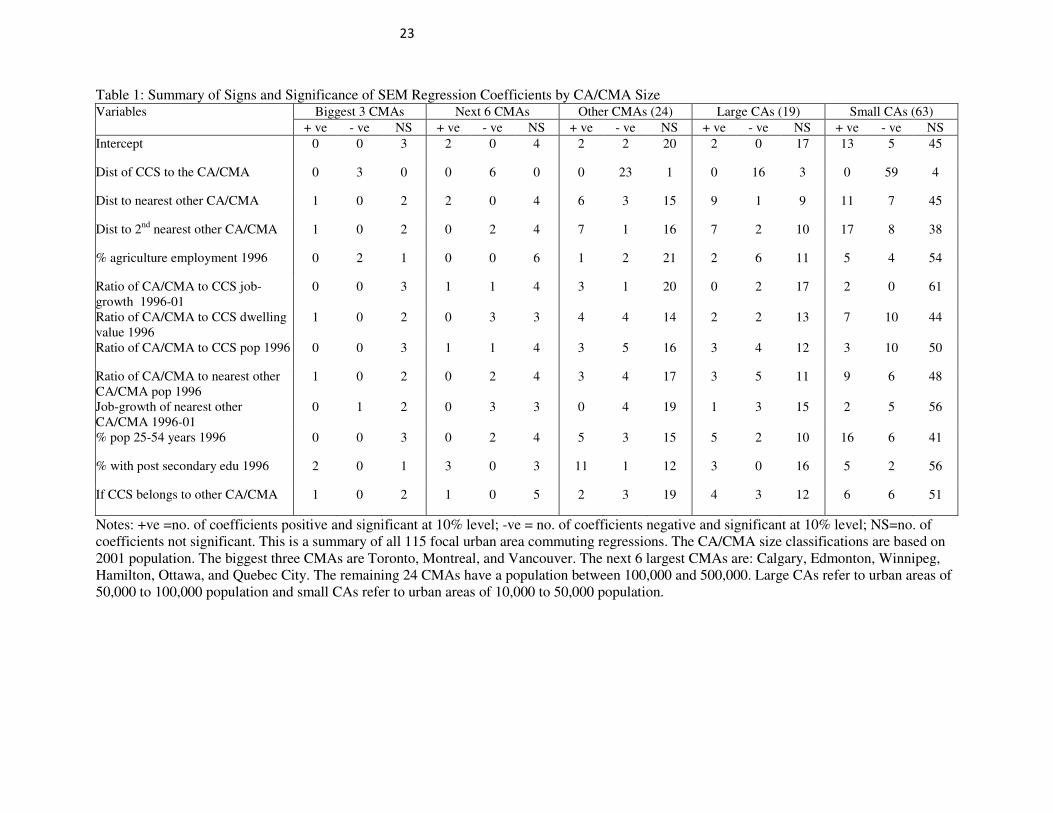
Given the apparent differences by size grouping, Table 1 reports a summary of the 115 coefficients

across different urban area sizes. The 115 models are divided into five samples. The top of Canada’s

urban hierarchy is comprised of Toronto, Montreal, and Vancouver, forming one group. The second

group is comprised of another 6 smaller centers that are above 500,000 in population. Together these two

groups of 'mega' urban centers have been referred to as the engines of growth for Canada (Partridge et al

2007b). The third group comprises an additional 24 centers that qualify for CMA designation of having a

core population of at least 100,000. The final two groups are derived by sub-dividing the sample of CAs

7By separating the regressions into separate urban area commuting models, we need not account for the correlated

error term structure that would result if we pooled overlapping commuting models together—i.e., the same CCS would appear more than once, which would create intractable econometric problems. Likewise, our use of a spatial error model also helps account for the spatial interdependence of overlapping commuting sheds.

12

12

at 50,000 residents to reflect different urban scales.

There are some common patterns across the samples with the distance to the focal urban area being

strongest example. Fully 107 out of the 115 distance coefficients are negative and statistically significant

at the 10% level, whereas the remaining 8 are insignificant. Yet, there clearly are idiosyncratic differences

among the 115 models in terms of significance. For example, while the vast majority of the cases where

either the distance to the nearest other urban area (besides the focal urban area) or the distance to the 2nd

closest urban area (besides the focal one) take on the expected positive sign, over 60% of these

coefficients are insignificant. This illustrates that the geographic scarcity of urban areas in Canada implies

fewer overlapping commuting sheds—though as shown below, this is not universal across the country.

The R-squared values (not shown) for the 115 models are consistently larger in the commuting

sheds centered on larger CA/CMAs, which suggests that there are more idiosyncratic effects surrounding

the smaller urban areas. This is also evident in the greater number of significant variables in the

commuting sheds centered on the larger urban centers. These observed differences by size of focal

CA/CMA are the basis of further analysis described below.

4.3 Model Aggregation

Estimation of individual models is informative in assessing commuting-shed relationships and in

providing empirical feedback for in-depth case studies. Still, the overall pattern across all commuting

sheds would be a useful benchmark for comparison. However, the volume of the results from the 115

models is too great to present and discuss in the window of a journal article. In addition, a pooled OLS

approach applied to the entire collection of CA/CMAs to summarize the results is inappropriate as a

significant number of CCS observations are included in more than one commuting shed. A simple

'stacking' of all the observations included in the 115 models would thus violate the independence of error

term assumption. Thus, we pursued a number of approaches to summarize the results and to provide an

assessment of regional differences across the country.

First, we undertook cluster analysis using the “Ward” method to help determine “like” CA/CMAs

for averaging or aggregating into regional aggregates. However, regardless of whether basing our

clustering on the estimated distance coefficients or the coefficients for all of the explanatory variables, the

cluster analysis did not uncover a coherent set of regions.

13

13

The ‘mean-group’ estimation was then selected as the preferred approach in deriving average

responses. The mean-group approach has been employed in the growth literature (Pesaran and Smith

1995; Pesaran et al. 1999). In their studies it involved estimating separate time-series regressions for each

of the cross-section units and then averaging each regression coefficient over all cross-section units.8 In

our case, individual commuting shed level models are the analogous cross-section regressions (though

they are not based on time-series data). Coefficients from these models are averaged for all CA/CMAs as

well as within each region. A common regionalization for Canada is the following 5 regions – British

Columbia (BC), Prairies (Alberta, Saskatchewan, and Manitoba), Ontario, Quebec, and Atlantic region

(Newfoundland, Prince Edward Island, Nova Scotia, and New Brunswick). This division renders 9

CA/CMAs in BC, 19 in the Prairies, 41 in Ontario, 29 in Quebec, and 17 in Atlantic Canada.

Rather than following the past mean-group practice of using unweighted averaging, our procedure

weights the coefficients by the respective population size of the focal point CA/CMA. This weighting

scheme allows the averaging to be representative of the population base. Other weighting procedures such

as using the population of the entire commuting shed were considered, but weighting by the CA/CMA

population produces stronger results (shown in Table 2).

4.4. Results by Region and Urban-Center Size

Table 2 shows the CA/CMA population-weighted results by region. Distance of the nonmetro area

from the urban center is consistently a strong predictor of the out-commuting rates. As expected, this

variable shows the negative impact of distance in all five regions indicating that the share of the

workforce that commutes to a given focal urban center declines with the distance from the center. This

impact is the strongest in Ontario, followed by Quebec, the Prairies, the Atlantic region, and BC. If the

communities’ average travel distance increases by 100 kms (about a one-hour drive), for example, the

average expected commuting rate declines by 22% in Ontario, 20% in Quebec and Prairies, 10% in

Atlantic region, and 7% in BC. The larger negative distance decay of commuting in Ontario and Quebec

is likely a simple artifact of the high commuting rates on the perimeters of their large urban centers,

forcing a more rapid descent to zero commuting rates at the 150 or 200km edge of commuting.

The average coefficient of distance to nearest other CA/CMA is statistically significant in Quebec

8Recent applications of this technique include Tan (2006) in case of foreign aid and growth, and Martinez and

Morancho (2004) in case of CO2 emissions and per capita income relationships.

14

14

and Prairie regions and the average coefficient of distance to second nearest other CA/CMA is

statistically significant only in Ontario. Both have the expected positive sign implying that if the nearest

or second nearest alternative urban center is farther away, then commuting rates to the focal CA/CMA

increases. In other words, all else equal, commuters are more likely to choose the nearest employment

center. Thus, in areas densely populated with urban centers, simple distance of a nonmetro community to

any particular urban center is an incomplete explanation of the commuting rate, requiring a consideration

of the broader spatial structure of urban centers (Thorsen and Gitlesen 1998; Ubøe 2004). These results

illustrate that in more densely settled regions, planning and infrastructure placement should consider how

agglomeration economies have a high geographical reach and that commuting sheds often overlap.

Figure 1 illustrates how competing urban areas alter commuting patterns. The figure shows the

percent of the local workforce that commutes to the London CMA, Ontario, which had a 2001 population

of 406,000. Rings are placed at 50kms, 100kms, and 150kms around its centroid. Then we add 3

additional rings: 1) 100km from the center of the Toronto CMA (4.7 million population in 2001); 2)

100km ring surrounding the Hamilton CMA (655,000 population in 2001); and 3) 100km ring

surrounding Windsor CMA, Ontario (297,000 people in 2001). The map clearly shows a discontinuous

increase in commuting rates into London from the east beyond a distance of 100kms from Toronto.

Likewise, commuting rates to the east take another discreet jump when Hamiliton is no longer within

100kms. Toward the west, commuting rates into London quickly fall below 5% when moving within

100kms of Windsor. In sum, commuting flows into London are greatly shaped by proximity to these other

competing urban areas. Similar interdependencies exist in any area densely populated with urban centers.

Among other variables, impacts of percent agricultural employment, job-growth ratio, and dwelling

value ratio are usually statistically insignificant. The statistical significance of distance and insignificance

of the focal urban area’s relative job growth suggest that access to urban employment is a greater

determinant of commuting rates than whether the urban area is growing. Perhaps if the dependent variable

were change in commuting rates over time, then relative job growth would play a more influential role.

The two population ratio variables are negative and significant (at 10% level) in only the Prairie

provinces. The insignificance of the agriculture employment share variable may simply reflect how the

distance variable coefficients are capturing the fact that agricultural intensity is related to remoteness.

Working age population of 25-54 years is positively associated with commuting rates, with the

15

15

exception of the Atlantic region. In the Prairie region, the impact is the strongest – a 1% increase in the

active age population is associated with an almost 1% increase in commuting rates. One implication is

that vibrant rural areas with a large prime working-age population are associated with more urban

commuting. Finally, the impact of education levels on commuting pattern is unexpectedly small for the

overall sample. The post secondary education variable is moderately positively associated with

commuting rates only in Quebec.

To examine the heterogeneity by urban center size, weighted coefficients are also presented for 5

size classes of CA/CMAs (Table 3). The size of the distance-to-nearest CA/CMA coefficient declines

monotonically across size groupings. This pattern is consistent with larger absolute commuting rates for

the largest cities, in which commuting rates ultimately decline to zero. Even though the point at which

commuting rates fall to zero is expected to be more distant for the largest centers, the much higher initial

rates would still require a steeper rate of decline for larger centers. For the two largest groups, as well as

CAs between 50 and 100k, the results support the expected positive influence of distance to competing

commuting destinations. For the largest 3 CA/CMA group, the post-secondary education variable now

has the expected positive sign. This may be indicative of the fact that only larger centers offer the types of

professional and highly skilled jobs that attract highly educated commuters from nearby nonmetro areas.

Further this would also be consistent with a deconcentration of this cohort to nearby nonmetro areas,

choosing a rural lifestyle while retaining professional jobs in the larger cities.

4.5. The Size of the Rural-Urban Footprint

The results of the predicted values of the commuting rates, for CA/CMA size groups is presented in

Figure 2 at three discrete distances from the core. These results begin to address three questions: (a) how

does distance from the urban center affect the predicted rates of decay in commuting rates, (b) how does

the CA/CMA population affect the decay, (c) what is the geographic size of the urban region’s footprint?

Figure 2 shows the average predicted commuting rates (%) at three discrete distances – 50, 100,

and 150km from the city center while all other variables are set to their mean values. The same 5 size

categories presented in Table 3 are depicted. The bar-graph shows monotonic distance decay of predicted

commuting rates for each size category at increased distances from the center. Further, with the exception

of the large CAs, there is also a monotonic ordering of predicted commuting rates across city sizes at each

distance. The predicted commuting rates are clearly much higher for the largest cities ranging, for

16

16

example, from 42% for the largest 3 cities at 50km to about 7% for the smallest urban centers. At 150km,

the predicted commuting rates from the largest group is still more than 20%, while for the smallest group

it has fallen to 2%. Thus although increased distance results in a greater decrease in commuting rates for

the largest centers, the absolute level of commuting rates is substantially higher for larger cities. The case

of the large CAs (50,000 - 100,000 population) merits further investigation because their commuting rates

are modestly greater than for the small CMAs. Yet, the 19 centers in this group are relatively isolated

from potentially competing core Canadian urban areas, which may affect commuting patterns.

Figure 3 shows three scatter plots of the predicted commuting rates (%) at 50, 100, and 150kms

distances based on all 115 individual commuting-shed models. The horizontal axis represents CA/CMA

population (in log scale). For example, at the far right, the two largest urban centers—Montreal and

Toronto—have by far the highest commuting rates at each three distance. To get a sense of the

distribution, three linear trend lines are fitted to the data. Their R2 values indicate that CA/CMA size

alone explains about 26-38% of the variation in the predicted commuting rates.

Figure 3 can help us ascertain the minimum urban size thresholds to achieve certain commuting

rates at each of these three distances. That is, what is the minimum urban size threshold such that rural

areas at 50, 100, and 150kms away would be expected to have a certain level of commuting rates with a

given focal urban area? Such urban size thresholds would be useful in planning for economic

development and infrastructure design. For illustration, the specific commuting thresholds we examine

are 30%+ for “strong” labor market linkages, 20%+ for “medium” labor market linkages and 10%+ for

“modest” labor market linkages. Though these commuting categories are somewhat arbitrary, they are

analogous to the metropolitan influence zone rates used by Statistics Canada and the corresponding urban

commuting influence used by the U.S. Department of Agriculture’s Economic Research Service.9

Figure 3 shows that a metropolitan area would need to be almost 2.5million population to have

strong labor market linkages with its rural areas that are 50kms away, 370,000 population to achieve

medium labor market linkages at that distance, and 55,000 population to achieve modest labor market

linkages.10

Of course, at distances closer than 50kms (100kms/150kms) the commuting rates are

9By comparison, the out-commuting rates used by Statistics Canada are 50% (Statistics Canada 2006) in

determining whether a locality is included in a metropolitan area, while the corresponding figure for the U.S. Census Bureau to include a county as part of a metropolitan area is 25% (U.S. Office of Management and Budget, 2000). 10

These figures are derived as the anti-log of the log population where the 50km line crosses the 30%, 20%, and 10% lines—i.e., exp(14.7), exp(12.8), and exp(10.9).

17

17

progressively higher. A metro area would need about 2.7 million to have medium linkages at a distance of

100kms and 165,000 to achieve modest labor market linkages at that distance. It would take about 2.0

million to garner a modest labor market attachment at 150kms. However, note that Montreal and Toronto

are outliers, where they nearly achieve strong labor market attachment even at 150kms. Therefore,

consistent with a gravity model, these results suggest that an urban area of about 55,000 people would

produce widespread economic effects on proximate rural areas in an 8,000km2 region (i.e., 50kms radius

is associated with almost 8,000km2), while a metropolitan area of 2.0 million would have expected effects

over an approximately 71,000km2 region. Note that these are average commuting effects, while

commuting rates and regional sizes are likely greater (smaller) when there is good (poor) transportation

access and fewer (more) competing urban destinations.

Figure 4 illustrates how these labor market areas overlap one another with the largest urban areas

generating the largest catchment areas, either fully or partially overlapping smaller regional labor market

areas. Specifically, it shows all of the CA/CMAs in Southern Ontario outlined in grey. It then shows rings

for the larger urban areas, for which the radius is determined by the distance at which predicted average

commuting rates fall to 10% using each urban area's regression model. Using this metric, Toronto's

commuting radius is 200kms and Montreal's commuting radius is 220kms, extending from Quebec into

Ontario. At the other extreme are smaller urban areas such as Kitchener, whose labor market region has a

predicted 55km radius. Interestingly, London's labor market region extends 165kms, which exceeds

Ottawa's 150kms, even though the Ottawa CMA is more than twice as populated. Yet, Ottawa's labor

market area is constrained on the east by Montreal and the west by Toronto, while Toronto is London's

only major competitor. Completely falling in Toronto's agglomeration shadow, note that Hamilton's reach

is only 75kms and Oshawa's is 30kms.11

A clear traditional urban hierarchy is also apparent in Figure 4. Toronto-at the top of the urban

hierarchy in Southern Ontario (and along with Montreal, in Quebec) has a geographical reach that fully or

partially overlaps 21 additional CAs and CMAs. Fully 29% of Canada's population falls in localities

covered by Toronto's labor market region. Secondary urban tiers in the Toronto region include Hamilton

and Kitchener, while even lower tiers are CA/CMAs without wide-ranging commuting sheds. Likewise,

11

The tangency of the Toronto and Ottawa labor market areas makes perfect economic sense as commuters would switch from location to the other. In fact, the prediction that they are tangent helps validate our empirical approach.

18

18

the figure validates the importance of Ottawa and Montreal as well as the relatively surprising importance

of London in Southwest Ontario.12

The patterns illustrate the rich overlapping nature of the urban

hierarchy in densely populated regions and why regional planners and development officials should

account for these broad interdependencies.

5. Concluding Remarks

Most commuting studies have focused on intra-urban areas. Yet, nonmetro to metro commuting is

evidence of the increasing spillovers that blur the distinction between rural and urban labor markets. Thus,

understanding commuting patterns surrounding urban centers improves our understanding of the evolving

nature of rural-urban interdependence, and informs local planning and governance matters. In appraising

this issue, a set of spatial error models was estimated for the broader regions surrounding 115 CA/CMAs

across Canada. The models were specified to identify push and pull factors to explain commuting

behavior across broad regions. Individual models for urban areas are estimated to account for

heterogeneity and econometric problems related to the existence of overlapping commuting sheds.

Summary results for five distinct economic regions and by five urban-area size categories are

presented in the form of weighted average coefficients of the individual focal urban area regressions.

Community distance from larger cities or job centers is the major predictor of commuting pattern in all

five regions and across the five metropolitan size categories. Invariably, the farther the community is

located from the urban center the lower the commuting rate, but the degree of reduction in commuting

varies across different regions with Ontario having the greatest distance decay. Likewise, the distance

decay of commuting rates was directly related to CA/CMA size, which relates to the extremely high

commuting rates in the most proximate communities. Conversely, relative job growth in the focal urban

center was insignificant, illustrating job access (as reflected through distance) is more important than

urban job growth in determining commuting levels. Yet, changes in commuting rates would be more

likely to be reflected in relative job growth rates.

Among other variables, the pool of working age population in the CCS showed a consistent

positive impact on out-commuting rates. Yet, average educational attainment plays a much stronger role

12

The emergence of the New Economic Geography (Krugman, 1991) has stimulated a recent investigation of the remarkable stability of the urban hierarchy in the face of significant declines in transportation costs, new innovations, and technological shocks, as well as considerable industry restructuring (of course, the emergence of GIS datasets has greatly facilitated this recent research). See Duranton (2007) for a recent example. Our current research further illustrates the overlapping nature of the urban system in driving integration of broad city-regions.

19

19

in describing commuting to CMAs (over 100,000 population), suggesting that commuting opportunities

in metropolitan areas may attract more educated individuals to the nearby rural areas. Also, from within

the rural labor force, commuters are self-selecting from the more educated cohorts.

Further analysis indicated that Canada’s two largest urban areas—Montreal and Toronto—exert a

huge economic footprint far outside their borders. However, even at the other end of the size spectrum,

metropolitan areas as small as 55,000 people can have a tangible impact over a region as large as 8,000

square kms, while a metropolitan area of 2.0 million would have tangible labor market linkages over

70,000 square km region. Clearly, this magnitude of spillovers indicates the need for considering urban

proximity in rural planning and economic development. Similarly, planning for urban development would

clearly benefit from acknowledging the magnitude of the rural labor market that is integrated with urban

economy and the underlying forces driving this interdependence.

The rural-urban interdependencies illustrated by the empirically estimated relationships represent

the functionally-integrated economic regions that have evolved as the labor market and population make

their place-of-residence and commuting decisions. The results also illustrate the overlapping nature of

these spatial linkages, especially in regions that are densely populated. Moreover, they illustrate the urban

hierarchy notions that the functional region will be larger, the higher the tier of the urban center, as well

as the nesting of lower-tiered areas within those of the higher-tiered centers.

Commuting inter-dependencies at the rural-urban interface are indicative of the de facto

regionalization that is occurring—though governance arrangements usually lag this process. The

particular pattern that is unique to each urban center is of local interest in policy and program design. In

addition, the broader patterns regarding the relationship between city size and the intensity and

geographic extent of commuting will inform the conceptualization of the role of urban agglomeration in

rural population growth and retention. Local and regional governance implications, as well as

infrastructure planning needs, also arise from these patterns.

20

20

References

Anderson, Anne Kaag. 2002. Are Commuting Areas Relevant for the Delimitation of Administrative Regions in Denmark? Regional Studies 38.8: 833-44.

Anselin, L. 1988. Spatial Econometrics: Methods and Models. Boston: Kluwer Academic Publishers.

Artis, M., J. Romani and J. Surinach. 2000. Determinants of Individual Commuting in Catalonia, 1961-91: Theory and Empirical Evidence. Urban Studies 37(8) 143-50.

Barkley, David L., Mark S. Henry, and Shuming Bao. 1996. Identifying “Spread” versus “Backwash” Effects in Regional Economic Areas: A Density Functions Approach. Land Economics 72 (3): 336-57. Berry, B.J.L 1961. A Method for Deriving Multi-factor Uniform Regions. Przegland Geofrahiczny 33: 263-82.

Berry, B.J.L 1968. Metropolitan Area Definition: A re-evaluation of Concept and Statistical Practice. Washington, DC: U.S. Bureau of the Census.

Berry, B.J.L. 1970. Commuting Patterns, Labor Market Participation and Regional Potential. Growth and Change 1(4): 3-10.

Cavailhès, Jean, Dominique Peeters, Evangelos Sékeris and Jacques-François Thisse. 2004. The Periurban City: Why to Live Between the Suburbs and the Countryside. Regional Science and Urban Economics 34: 681-703.

du Plessis, Valerie, Roland Beshiri, Ray D. Bollman, and Heather Clemenson. 2002. Definition of Rural. Agriculture and Rural Working Paper Series Working Paper No. 61 (series 21-601-MIE). Accessed from www.statcan.ca.

Duranton, Gilles, 2007. Urban Evolutions: The Fast, the Slow, and the Still. American Economic Review 97(1): 197-221.

Eliasson, Kent, Urban Lindgren and Olle Westerlund. 2003. Geographical Labour Mobility: Migration or Commuting? Regional Studies 37.8: 827-37.

Fox, K.A., and T.K. Kumar. 1965. The Functional Economic Area: Delineation and Implications for Policy Analysis. Papers of the Regional Science Association 15: 57-85.

Gaile, G.L. 1980. “The Spread-Backwash Concept.” Regional Studies 14 (1): 15-25.

Glaeser, Edward L. and Matthew E. Kahn. 2003. Sprawl and Urban Growth. NBER Working Paper Series 9733.

Green, M.B. and S.P. Meyer. 1997. An Overview of Commuting in Canada with Special Emphasis on Rural Commuting and Employment. Journal of Rural Studies 13(2): 163-75.

Henry, Mark S., David L Barkley and Shuming Bao. 1997. The Hinterland's Stake in Metropolitan Growth: Evidence from Selected Southern Regions. Journal of Regional Science 37(3): 479-501.

Hu, P. and J. Pooler. 2002. An Empirical Test of the Competing Destinations Model. Journal of Geographical Systems 4: 301-23.

Hughes, David W. and David W. Holland. 1994. Core-Periphery Economic Linkage: A Measure of Spread and Possible Backwash Effects for the Washington Economy. Land Economics 70(3): 364-77.

Krugman, P., 1991. Increasing Returns and Economic Geography. Journal of Political Economy 99: 483-499.

21

21

Martinez-Zarzoso, I. and A. Bengochea-Morancho. 2004. Pooled Mean-Group Estimation of an Environmental Kuznets Curve for CO2. Economic Letters 82: 121-26.

McKee, David L. and Yosra A. McKee. 2004. Edge Cities, Urban Corridors and Beyond. International Journal of Social Economics 31(5/6): 536-43.

Mitchell, Clare J. 2005. Population Change and External Commuting in Canada’s Rural and Small Town Municipalities. Canadian Journal of Regional Science 28(3): 461-86.

Mitchelson, R.L., and J.S. Fisher. 1981. Extended and Internal Commuting in the Transformation of the Intermetropolitan Periphery. Economic Geography 57: 189-207.

Mitchelson, R.L., and J.S. Fisher. 1987. Long-distance commuting and population change in Georgia, 1960-80. Growth and Change 18(1): 44-65.

Moss, Joan E., Claire G. Jack and Michael T. Wallace. 2004. Employment Location and Associated Commuting Patterns for Individuals in Disadvantaged Rural Areas in Northern Ireland. Regional Studies 38.2: 121-36.

Nechyba, Thomas J. and Randall P. Walsh. 2004. “Urban Sprawl.” Journal of Economic Perspectives 18: 177-200.

Olfert, M. Rose and Jack C. Stabler. 1998. Spatial Dimensions of Rural, Gender Specific Labour Force Commuting Patterns. Australasian Journal of Regional Studies 4(2): 253-74.

Partridge, Jamie and James Nolan. 2005. Commuting on the Canadian Prairies and the Urban/Rural Divide. Canadian Journal of Administrative Sciences 22(1): 58-72.

Partridge, Mark, Ray D. Bollman, M. Rose Olfert and Alasia Alessandro. 2007a. Riding the Wave of Urban Growth in the Countryside: Spread, Backwash, or Stagnation? Land Economics 83(2): 128-52.

Partridge, Mark, M. Rose Olfert and Alasia Alessandro. 2007b. Canadian Cities as Regional Engines of Growth. Canadian Journal of Economics 40(1): 39-68.

Pesaran, M.H. and R. Smith. 1995. Estimating Long-Run Relationships from Dynamic Heterogeneous Panels. Journal of Econometrics 68: 79-113.

Pesaran, M.H., Y. Shin and R.P. Smith. 1999. Pooled Mean Group Estimation of Dynamic Heterogeneous Panels. Journal of the American Statistical Association 94(446): 621-34.

Renkow, M. and D. Hoover. 2000. Commuting, Migration, and Rural-Urban Population Dynamics. Journal of Regional Science 40(2): 261-87.

Renkow, M. 2003. Employment Growth, Worker Mobility, and Rural Economic Development. American Journal of Agricultural Economics 85(2): 503-13.

Rouwendal, Jan. 1999. Spatial Job Search and Commuting Distances. Regional Science and Urban Economics 29: 491-517.

Rouwendal, Jan and Erik Meijer. 2001. Preferences for Housing, Jobs and Commuting: A Mixed Logit Analysis. Journal of Regional Science 41(3): 475-505.

Schmitt, Bertrand, Mark S. Henry, Virginie Piguet and Mohamed Hilal. 2006. Urban Growth Effects on Rural Population, Export and Service Employment: Evidence from Eastern France. Annals of Regional Science 40: 779-801.

So, K.S., P.F. Orazem and D.M. Otto. 2001. The Effects of Housing Prices, Wages, and Commuting

22

22

Time on Joint Residential and Job Location Choices. American Journal of Agricultural Economics 83(4): 1036-48.

Song, S. 1994. Modeling Worker Residence Distribution in the Los Angeles Region. Urban Studies 31(9): 1533-44.

Stabler, Jack C., M. Rose Olfert and Jonathan B. Greuel. 1996. Spatial Labor Markets and the Rural Labor Force. Growth and Change 27(2): 206-30.

Statistics Canada. Censuses of Population 1851-2001. Accessed at: http://www40.statcan.ca/l01/cst01/demo62a.htm

Statistics Canada 2004. 2001 Census Dictionary-internet version. Catalogue no. 92-378-XIE, p. 230-231.

Tan, K.Y. 2006. A Pooled Mean Group Analysis on Aid and Growth. CSAE WPS/2006-14. Department of Economics, University of Oxford, U.K.

Thorsen, Inge and Jens Petter Gitlesen. 1998. Empirical Evaluation of Alternative Model Specifications to Predict Commuting Flows. Journal of Regional Science 38(2): 273-92.

Ubøe, Jan. 2004. Aggregation of Gravity Models for Journeys to Work. Environment and Planning A 36: 715-29.

U.S. Census Bureau. Selected Historical Decennial Census Population and Housing Counts. Accessed at: http://www.census.gov/population/www/censusdata/hiscendata.html.

U.S. Office of Management and Budget 2000. Federal Register 65(249), December 27, p.82236.

23

23

Table 1: Summary of Signs and Significance of SEM Regression Coefficients by CA/CMA Size Variables Biggest 3 CMAs Next 6 CMAs Other CMAs (24) Large CAs (19) Small CAs (63)

+ ve - ve NS + ve - ve NS + ve - ve NS + ve - ve NS + ve - ve NS

Intercept 0 0 3 2 0 4 2 2 20 2 0 17 13 5 45

Dist of CCS to the CA/CMA 0 3 0 0 6 0 0 23 1 0 16 3 0 59 4

Dist to nearest other CA/CMA 1 0 2 2 0 4 6 3 15 9 1 9 11 7 45

Dist to 2nd

nearest other CA/CMA 1 0 2 0 2 4 7 1 16 7 2 10 17 8 38

% agriculture employment 1996 0 2 1 0 0 6 1 2 21 2 6 11 5 4 54

Ratio of CA/CMA to CCS job-

growth 1996-01

0 0 3 1 1 4 3 1 20 0 2 17 2 0 61

Ratio of CA/CMA to CCS dwelling

value 1996

1 0 2 0 3 3 4 4 14 2 2 13 7 10 44

Ratio of CA/CMA to CCS pop 1996 0 0 3 1 1 4 3 5 16 3 4 12 3 10 50

Ratio of CA/CMA to nearest other

CA/CMA pop 1996

1 0 2 0 2 4 3 4 17 3 5 11 9 6 48

Job-growth of nearest other

CA/CMA 1996-01

0 1 2 0 3 3 0 4 19 1 3 15 2 5 56

% pop 25-54 years 1996 0 0 3 0 2 4 5 3 15 5 2 10 16 6 41

% with post secondary edu 1996 2 0 1 3 0 3 11 1 12 3 0 16 5 2 56

If CCS belongs to other CA/CMA 1 0 2 1 0 5 2 3 19 4 3 12 6 6 51

Notes: +ve =no. of coefficients positive and significant at 10% level; -ve = no. of coefficients negative and significant at 10% level; NS=no. of

coefficients not significant. This is a summary of all 115 focal urban area commuting regressions. The CA/CMA size classifications are based on

2001 population. The biggest three CMAs are Toronto, Montreal, and Vancouver. The next 6 largest CMAs are: Calgary, Edmonton, Winnipeg,

Hamilton, Ottawa, and Quebec City. The remaining 24 CMAs have a population between 100,000 and 500,000. Large CAs refer to urban areas of

50,000 to 100,000 population and small CAs refer to urban areas of 10,000 to 50,000 population.

24

24

Table 2: Weighted Average Coefficients and t-values (in parentheses) for Out-commuting Rates by

Economic Regions Variables British Columbia Prairies Ontario Quebec Atlantic

Intercept

Dist of CCS to the CA/CMA

Dist to nearest other CA/CMA

Dist to 2nd

nearest other CA/CMA

% agriculture employment 1996

Ratio of CA/CMA to CCS job-

growth 1996-01

Ratio of CA/CMA to CCS dwelling

value 1996

Ratio of CA/CMA to CCS pop 1996

Ratio of CA/CMA to nearest other

CA/CMA pop 1996

Job-growth of nearest other CA/CMA

1996-01

% pop 25-54 years 1996

% with post secondary edu 1996

If CCS belongs to other CA/CMA

-3.207

(-0.09)

-0.065**

(-2.36)

-0.032

(-0.60)

0.047

(0.93)

-0.034

(-0.15)

-0.951

(-1.21)

-0.934

(-0.25)

-3.620

(-0.55)

9.565

(0.74)

0.181

(0.76)

0.332

(0.88)

-0.030

(-0.19)

-0.807

(-0.31)

166.307*

(1.95)

-0.198**

(-5.65)

0.113*

(1.75)

-0.062

(-1.22)

0.246

(1.16)

-0.293

(-0.43)

6.827

(1.41)

-51.745*

(-1.89)

-88.281*

(-1.83)

-1.330*

(-1.94)

1.362**

(2.00)

-0.063

(-0.29)

-7.160

(-1.38)

20.320

(0.83)

-0.216**

(-8.53)

0.050

(1.11)

0.105**

(2.42)

-0.088

(-1.22)

0.005

(0.02)

-1.641

(-0.94)

0.863

(0.32)

2.993

(0.44)

0.019

(0.19)

0.444**

(2.65)

0.018

(0.30)

-1.980

(-1.43)

29.050

(0.96)

-0.198**

(-9.10)

0.082**

(2.34)

0.040

(1.09)

-0.060

(-1.63)

-0.133

(-0.33)

-0.942

(-0.96)

1.917

(1.11)

4.197

(0.62)

0.136*

(1.70)

0.156*

(1.70)

0.062*

(1.71)

-1.092

(-1.00)

4.692

(0.18)

-0.099**

(-4.11)

0.042

(0.98)

0.001

(0.01)

0.006

(0.03)

0.222

(0.55)

-2.463

(-1.21)

3.498

(0.84)

-3.877

(-0.25)

0.044

(0.21)

0.277

(1.15)

-0.008

(-0.11)

-0.535

(-0.25)

No. of CA/CMAs 9 19 41 29 17

Notes: Individual CA/CMA specific out-commuting rate regressions are estimated following specification of spatial

error models in (5) and the coefficients and standard errors are averaged over the number of CA/CMAs in each

region using populations of the CA/CMAs as weights. A ** or * indicates significant at 5% or 10% level

respectively.

25

25

Table 3: Weighted Average Coefficients and t-values (in parentheses) for Out-commuting Rates 2001 by

CA/CMA Size Variables Biggest 3 CMAs Next 6 CMAs Other CMAs Large CAs Small CAs

Intercept

Dist of CCS to the CA/CMA

Dist to nearest other CA/CMA

Dist to 2nd

nearest other CA/CMA

% agriculture employment 1996

Ratio of CA/CMA to CCS job-

growth 1996-01

Ratio of CA/CMA to CCS dwelling

value 1996

Ratio of CA/CMA to CCS pop 1996

Ratio of CA/CMA to nearest other

CA/CMA pop 1996

Job-growth of nearest other CA/CMA

1996-01

% pop 25-54 years 1996

% with post secondary edu 1996

If CCS belongs to other CA/CMA

30.977

(0.97)

-0.242**

(-8.35)

0.061

(1.23)

0.116**

(2.35)

-0.148

(-1.61)

-0.159

(-1.05)

0.125

(1.06)

-2.605

(-1.45)

1.265

(0.41)

-1.441

(-0.91)

4.708

(0.66)

0.417**

(2.15)

0.022

(0.29)

126.448*

(1.93)

-0.209**

(-6.73)

0.104*

(1.84)

-0.037

(-0.78)

0.183

(1.13)

-0.059

(-0.29)

-0.925**

(-2.10)

4.451

(1.18)

-37.115*

(-1.93)

-5.708

(-1.58)

-60.237*

(-1.81)

1.001**

(2.01)

-0.016

(-0.10)

-3.872

(-0.16)

-0.109**

(-5.33)

0.012

(0.27)

0.040

(1.01)

0.035

(0.28)

-0.302

(-0.65)

0.040

(0.25)

0.232

(0.10)

-0.543

(-0.13)

-2.119

(-1.15)

3.055

(0.30)

0.405*

(1.81)

0.024

(0.32)

13.290

(0.61)

-0.101**

(-4.52)

0.071**

(1.99)

0.002

(0.07)

-0.022

(-0.26)

0.035

(0.02)

0.003

(0.03)

-0.251

(-0.12)

2.777

(0.73)

-0.116

(-0.06)

-2.678

(-0.33)

0.105

(0.64)

-0.040

(-0.61)

2.393

(0.10)

-0.061**

(-4.05)

0.016

(0.65)

0.008

(0.37)

0.002

(0.04)

-0.402

(-0.26)

-0.017

(-0.07)

-0.081

(-0.06)

1.219

(0.43)

-0.565

(-0.40)

2.844

(0.16)

0.066

(0.58)

-0.001

(-0.02)

No. of CA/CMAs 3 6 24 19 63

Notes: Individual CA/CMA specific out-commuting rate regressions are estimated following specification of spatial

error models in (5) and the coefficients and standard errors are averaged over the number of CA/CMAs in each

group using populations of the CA/CMAs as weights. A ** or * indicates significant at 5% or 10% level

respectively. See notes to Table 1 for details of the CA/CMA size classifications.

26

26

Figure 1: Competing Urban Centers and Overlapping Commuting Sheds of London CMA, Ontario.

27

27

Figure 2: Distance Decay of Predicted Commuting Rates by Five CA/CMA Size Categories

0.00

5.00

10.00

15.00

20.00

25.00

30.00

35.00

40.00

45.00

At50km At100km At150km

Av

era

ge

Pre

dic

ted

Co

mm

uti

ng

Ra

tes

(%)

Biggest 3 CMAs Next 6 CMAs Other CMAs Large CAs Small CAs

See notes to Table 1 for details of the CA/CMA size classifications.

Figure 3: CA/CMA Size and Predicted Commuting Rate Gradients at Select Distances

y = 5.226x - 47

R² = 0.375

y = 3.590x - 33.15

R² = 0.370

y = 1.975x - 18.66

R² = 0.262

0.00

10.00

20.00

30.00

40.00

50.00

60.00

9.2 10.2 11.2 12.2 13.2 14.2 15.2

Pre

dic

ted

Co

mm

uti

ng

Ra

tes

(%)

log(CA or CMA Population Size)

At50km At100km At150km Linear (At50km) Linear (At100km) Linear (At150km)

28

28

Figure 4: Overlapping Labor Markets Reflecting Urban Hierarchy in Southern Ontario.

Note: Other CA/CMAs without defined labor market areas are shown, but not labeled.

29

29

Appendix Table 1: Variable Definitions and Descriptive Statistics of the 115 Commuting Sheds

Variable Description Source Mean St. dev.

Commuting rate to CA/CMA 2001(dependent variable)

Percent workers commuting to an urban center (CA/CMA) for jobs from rural CCS in 2001

2001 Census 1.60 6.39

Dist of CCS to the CA/CMA Distance (in km) between the centroids of CCS and the focal CA/CMA

C-RERL 116.94 48.84

Dist to nearest other

CA/CMA

Distance between the centroids of CCS and nearest other (than the focal) CA/CMA

Authors’ calculation

37.44 31.06

Dist to 2nd

nearest other

CA/CMA

Distance between the centroids of CCS and 2nd

nearest other (than the focal and nearest other) CA/CMA

Authors’ calculation

64.20 41.98

% agriculture employment

1996

Percent of CCS workforce employed in agriculture sector 1996

1996 Census 10.97 12.43

Ratio of CA/CMA to CCS job-growth 1996-01

Ratio of employment growth in the focal CA/CMA over 1996-2001 to that of the CCS

1996, 2001 Censuses

0.71 6.70

Ratio of CA/CMA to CCS dwelling value 1996

Ratio of the value of dwelling units in the focal CA/CMA to that of the CCS 1996

1996 Census 1.25 0.5

Ratio of CA/CMA to CCS

pop 1996

Ratio of the log (population of the focal CA/CMA) to that of the CCS 1996

1996 Census 1.41 0.28

Ratio of CA/CMA to nearest other CA/CMA pop 1996

Ratio of the log(pop of the focal CA/CMA) to that of the nearest other CA/CMA 1996

1996 Census 1.00 0.60

Job-growth of nearest other

CA/CMA 1996-01

Employment growth (%) of the nearest other (than the focal) CA/CMA over 1996-2001

1996, 2001 Censuses

4.98 7.37

% pop 25-54 years 1996

Percent of CCS population of age 25-54 years 1996

1996 Census 43.56 4.14

% with post secondary education 1996

Percent of CCS population of age 25-54 years that have post-secondary education 1996

1996 Census 48.85 10.17

If CCS belongs to other CA/CMA

A dummy variable with a value of 1 if the CCS is part of an urban center (CA/CMA); 0 if rural

Authors’ calculation

0.24 0.43

No. of obs. in 115 CA/CMA Commuting Sheds

23,019

Note: there are 2,607 CCSs in Canada, but the 115 focal urban area samples have considerable overlap. C-RERL = Canada Rural Economy Research Lab, University of Saskatchewan.

30

30

Appendix Table 2: Spatial Error Model Coefficients and t-values (in parentheses) of Out-commuting Rates to Select CA/CMAs 2001 by Economic

Regions Regions British Columbia Prairies Ontario Quebec Atlantic

Variables\Cities Vancouver Powell River Calgary Estevan Toronto Simcoe Montreal Lachute Halifax Gander

Intercept

Dist of CCS to the CA/CMA

Dist to nearest other CA/CMA

Dist to 2nd

nearest other CA/CMA

% agriculture employment 1996

Ratio of CA/CMA to CCS job-

growth 1996-01

Ratio of CA/CMA to CCS dwelling

value 1996

Ratio of CA/CMA to CCS pop 1996

Ratio of CA/CMA to nearest other

CA/CMA pop 1996

Job-growth of nearest other

CA/CMA 1996-01

% pop 25-54 years 1996

% with post secondary edu 1996

If CCS belongs to other CA/CMA

10.676

(0.30)

-0.060*

(-1.91)

-0.007

(-0.13)

0.020

(0.40)

-0.175

(-0.83)

-0.694

(-1.17)

-4.990

(-1.49)

-4.865

(-0.78)

15.140

(1.11)

0.320

(1.45)

0.132

(0.36)

-0.089

(-0.54)

1.331

(0.52)

-0.242

(-1.22)

-0.001**

(-4.62)

-0.001

(-1.36)

0.001

(1.02)

0.001

(0.33)

0.004

(0.24)

0.022

(0.54)

0.112

(1.37)

0.087

(0.80)

-0.002

(-1.23)

0.000

(0.13)

0.003**

(2.20)

0.065**

(2.45)

139.67**

(3.76)

-0.195**

(-9.27)

0.219**

(5.80)

-0.125**

(-4.01)

0.144

(1.13)

0.064

(0.65)

5.351

(1.59)

-49.61**

(-3.67)

-45.186*

(-1.75)

-1.201**

(-5.94)

0.556

(0.98)

-0.077

(-0.36)

3.562

(0.88)

34.88*

(1.95)

-0.024

(-0.59)

0.059

(1.28)

0.035

(0.98)

0.031

(0.39)

-1.545

(-0.83)

-1.759**

(-2.47)

-9.026

(-0.94)

-33.99**

(-2.28)

-0.670**

(-2.70)

0.253

(1.27)

-0.046

(-0.72)

-2.557

(-0.54)

33.413

(1.08)

-0.307**

(-10.15)

0.066

(1.23)

0.204**

(3.91)

-0.175**

(-2.17)

-0.015

(-0.30)

-2.741

(-1.62)

2.609

(0.99)

-0.274

(-0.04)

-0.015

(-0.13)

0.689**

(3.68)

0.024

(0.35)

-2.389*

(-1.65)

-1.613

(-0.36)

-0.031**

(-5.21)

0.011

(0.79)

0.023*

(1.68)

0.054**

(2.25)

-0.025

(-0.52)

-0.470

(-0.56)

-4.334**

(-2.79)

5.317**

(2.38)

0.048*

(1.81)

0.073

(1.13)

0.040*

(1.82)

-0.567

(-1.40)

39.442

(1.28)

-0.259**

(-9.98)

0.093**

(2.21)

0.050

(1.12)

-0.094**

(-2.52)

-0.045

(-1.42)

-1.030

(-1.01)

2.986*

(1.68)

5.486

(1.28)

0.203**

(2.93)

0.208**

(2.04)

0.085**

(2.09)

-1.752

(-1.47)

3.288

(0.89)

-0.024**

(-3.01)

-0.022*

(-1.94)

0.019

(1.60)

0.000

(-0.01)

0.000

(0.01)

0.660

(1.25)

-0.353

(-0.39)

1.772

(0.86)

-0.028

(-1.07)

-0.018

(-0.55)

-0.004

(-0.32)

-0.172

(-0.53)

31.195

(1.42)

-0.165**

(-6.60)

0.060

(1.36)

-0.029

(-0.80)

0.024

(0.23)

-0.134

(-1.08)

-4.104**

(-2.23)

0.053

(0.02)

-21.468*

(-1.77)

0.238

(1.13)

0.587**

(2.53)

0.041

(0.49)

-2.293

(-1.20)

266.91*

(1.72)

-0.090**

(-4.85)

-0.006

(-0.44)

0.040*

(1.91)

-0.349

(-1.10)

0.444

(0.46)

0.544

(0.37)

-1.016

(-0.16)

-302.43

(-1.63)

-5.094*

(-1.73)

-0.077

(-0.27)

0.053

(0.73)

-5.035

(-1.14)

Spatial autocorrelation coefficient

Adjusted R2

No. of CCSs within 200 km radius

No. of CCSs included in model est.

CCSs do not commute to this city

0.898**

(18.79)

0.76

37

28

0%

-0.896**

(-3.14)

0.55

34

33

67%

-0.989**

(-3.07)

0.78

29

25

4%

0.745**

(5.44)

0.44

80

79

81%

0.984**

(92.37)

0.73

263

227

9%

0.910**

(16.93)

0.30

195

193

90%

0.989**

(138.10)

0.76

587

494

25%

0.941**

(13.18)

0.16

551

502

95%

0.526**

(3.60)

0.43

113

105

56%

0.285

(1.27)

0.35

57

54

63%

Notes: Results for the largest (CMA) and smallest (CA) cities in each region are shown. A ** or * indicates significant at 5% or 10% level respectively.