urban form and activity-travel patterns - tu/e
TRANSCRIPT

URBAN FORM AND ACTIVITY-TRAVEL PATTERNS
AN ACTIVITY-BASED APPROACH TO
TRAVEL IN A SPATIAL CONTEXT
PROEFSCHRIFT
ter verkrijging van de graad van doctor aan de
Technische Universiteit Eindhoven, op gezag van de
Rector Magnificus, prof.dr. R.A. van Santen, voor een
commissie aangewezen door het College voor
Promoties in het openbaar te verdedigen op
23 januari 2002 om 16.00 uur
door
Daniëlle Maria Elisabeth Gertrudis Wilhelmine Snellen
geboren te Weert

Dit proefschrift is goedgekeurd door de promotoren:
prof.dr. H.J.P. Timmermans
en
prof.dr.ing. K.W. Axhausen, M.S.
omslag ontwerp Tekenstudio Faculteit Bouwkunde
foto omslag Gemeente Woerden
druk Universiteitsdrukkerij Technische Universiteit Eindhoven
ISBN 90-6814-562-2
© 2001, Technische Universiteit Eindhoven, Faculteit Bouwkunde, Capaciteitsgroep
Stedebouw, en de auteur, Daniëlle Snellen

PREFACE
Urban planning and design, to me, are fascinating fields of work. They are present
anytime and anywhere, they shape the world we live in and offer us a land of
opportunities (and some constraints). They combine both functional and aesthetical
considerations and, given the expected life span of the product, always require a
sustainable approach. The aesthetics of urban design I like to experience in my leisure
time. I can really enjoy walking through a beautiful old city, a new residential
development, a spacious square, or a compact mixed use centre full of people. My
professional focus in urban planning, however, is more on the functional side. How do
people cope with their spatial environment? How does it influence people’s options and
choices? Through the years, the way people travel in a spatial context has become the
main subject of my interest. In 1995, this interest resulted in the start of a PhD project.
Doing a PhD is a job that takes you through ups and downs, through periods of
confidence and times of doubt, wondering whether you will ever finish. In the last six
years, many people have stood by me and every single one of them has contributed in
some way or another to the result you see before you.
First of all I would like to thank Harry Timmermans for giving me the opportunity to
develop my own research proposal. I very much appreciate the confidence he placed in
me, the freedom I was given to develop the project and the support he gave me through
the years. Without his encouragement and advice, there would be no thesis for which
to write a preface. I am also very grateful to my second advisor Kay Axhausen. His
careful and accurate review of the manuscript resulted in insightful and useful
comments that have enhanced the quality of my work. His contribution is greatly
appreciated. Furthermore, I would like to express my gratitude to Aloys Borgers. From
the very beginning he has been an important support. He was always there to answer my
questions, to discuss problems and to help me in choosing directions during the
process. He has made valuable contributions to my work.
The urban planning group has provided a wonderful environment for doing my PhD.
They offered both social, psychological and scientific support. The amicable atmosphere,
Urban Form and Activity-Travel Patterns __________________________________________
-ii-
the weekly coffee meetings with cake and the sports group all contributed to this. My
special thanks go out to my roommates through the years, especially to Maarten Ponjé,
who held out longest with me. Ups and downs, both of the mind and of the work, all
found their place in room 5.04. Furthermore, I would like to thank Astrid Kemperman
for the good times we had in supervising our second year students and for the good
example she set last year. Also a warm thank you to Mandy van de Sande-van Kasteren,
for being the most wonderful secretary in the world and doing so much without even
being asked. Thanks to Leo van Veghel, for the stack of books and papers he organised
for me. And finally, my roommate, and later on, neighbour, Peter van der Waerden,
thanks for all the support, advice (there are two options ....) and many cups of coffee.
People outside the university community have also been an enormous support. The
interest in my PhD project of my SGBO colleagues has meant a lot to me in the final
year of finishing the thesis. To my friends and family, thank you all for being there for
me and providing the much needed variety. Your e-mails, visits and phone calls, our
weekends at home and away, self-indulging days in the thermae, Sunday morning
breakfasts, enjoyable evenings and BBQ’s all have a special meaning to me. A special
thank you goes out to my parents, for raising me to be the independent woman I am
now. Thanks Mam, for supporting my choices.
Finally, I would like to thank the person most important to me. Wouter, you have stood
by me, encouraged me, you sheered me up in hard times and shared my joy in good
times. Your support, patience and sometimes endurance have been crucial in the last six
years. Thank you, I love you.
Daniëlle Snellen
November 2001

-iii-
TABLE OF CONTENTS
PREFACE . . . . . . . . . . . . . . . . . . . . . . . . . . . . . . . . . . . . . . . . . . . . . . . . . . . . . . . . . . . . . i
TABLE OF CONTENTS . . . . . . . . . . . . . . . . . . . . . . . . . . . . . . . . . . . . . . . . . . . . . . . . . iii
LIST OF TABLES . . . . . . . . . . . . . . . . . . . . . . . . . . . . . . . . . . . . . . . . . . . . . . . . . . . . . vii
LIST OF FIGURES . . . . . . . . . . . . . . . . . . . . . . . . . . . . . . . . . . . . . . . . . . . . . . . . . . . . . ix
1 | INTRODUCTION . . . . . . . . . . . . . . . . . . . . . . . . . . . . . . . . . . . . . . . . . . . . . . . . . . . 1
1.1 Background . . . . . . . . . . . . . . . . . . . . . . . . . . . . . . . . . . . . . . . . . . . . . . . . . 1
1.2 Aims, Objectives and Basic Approach . . . . . . . . . . . . . . . . . . . . . . . . . . . 2
1.3 Organisation of the Thesis . . . . . . . . . . . . . . . . . . . . . . . . . . . . . . . . . . . . . 3
2 | DUTCH POLICY BACKGROUND . . . . . . . . . . . . . . . . . . . . . . . . . . . . . . . . . . . . . . 5
2.1 Introduction . . . . . . . . . . . . . . . . . . . . . . . . . . . . . . . . . . . . . . . . . . . . . . . . . 5
2.2 The Mobility Issue . . . . . . . . . . . . . . . . . . . . . . . . . . . . . . . . . . . . . . . . . . . . 5
2.3 National Spatial Mobility Policy . . . . . . . . . . . . . . . . . . . . . . . . . . . . . . . . 8
2.3.1 Mobility Policies from a Spatial Planning Perspective 1960-1990 8
2.3.2 Spatial Policies from a Transportation Planning Perspective 1979-
1995 . . . . . . . . . . . . . . . . . . . . . . . . . . . . . . . . . . . . . . . . . . . . . . . . . 11
2.3.3 Developments in Dutch Spatial Mobility Policy . . . . . . . . . . . . . . . 15
2.4 Spatial Policy and Mobility on the Local Scale . . . . . . . . . . . . . . . . . . . . 17
2.4.1 Elaboration of the Second Transport Structure Scheme for the City
Level . . . . . . . . . . . . . . . . . . . . . . . . . . . . . . . . . . . . . . . . . . . . . . . . 17
2.4.2 Instrument for Measuring Local Traffic Performance . . . . . . . 19
2.5 Conclusions . . . . . . . . . . . . . . . . . . . . . . . . . . . . . . . . . . . . . . . . . . . . . . . 19

Urban Form and Activity-Travel Patterns __________________________________________
-iv-
3 | TRAVEL AND ITS SPATIAL CONTEXT . . . . . . . . . . . . . . . . . . . . . . . . . . . . . . . . . 21
3.1 Introduction . . . . . . . . . . . . . . . . . . . . . . . . . . . . . . . . . . . . . . . . . . . . . . . . 21
3.2 Theoretical Discussions . . . . . . . . . . . . . . . . . . . . . . . . . . . . . . . . . . . . . 22
3.3 Model Simulations . . . . . . . . . . . . . . . . . . . . . . . . . . . . . . . . . . . . . . . . . 24
3.4 Empirical Studies . . . . . . . . . . . . . . . . . . . . . . . . . . . . . . . . . . . . . . . . . . 27
3.4.1 The Region as the Unit of Observation . . . . . . . . . . . . . . . . . . . 28
3.4.2 The City as the Unit of Observation . . . . . . . . . . . . . . . . . . . . . . 30
3.4.3 The Neighbourhood as the Unit of Observation . . . . . . . . . . . . 32
3.5 Conclusions and Discussion . . . . . . . . . . . . . . . . . . . . . . . . . . . . . . . . . 40
4 | RESEARCH DESIGN . . . . . . . . . . . . . . . . . . . . . . . . . . . . . . . . . . . . . . . . . . . . . . 42
4.1 Introduction . . . . . . . . . . . . . . . . . . . . . . . . . . . . . . . . . . . . . . . . . . . . . . . 42
4.2 Conceptual Framework: An Activity-Based Approach . . . . . . . . . . . . . . 43
4.3 Methodological Principles . . . . . . . . . . . . . . . . . . . . . . . . . . . . . . . . . . . 46
4.3.1 Quasi-Experimental Design Data . . . . . . . . . . . . . . . . . . . . . . . . 46
4.3.2 Controlling for Bias Due to Scale Differences . . . . . . . . . . . . . . 47
4.3.3 Avoiding Partial Analysis . . . . . . . . . . . . . . . . . . . . . . . . . . . . . . 49
4.3.4 Avoiding Under-Reporting of Trips . . . . . . . . . . . . . . . . . . . . . . 50
4.4 Conclusions . . . . . . . . . . . . . . . . . . . . . . . . . . . . . . . . . . . . . . . . . . . . . . . . 52
5 | DATA ISSUES . . . . . . . . . . . . . . . . . . . . . . . . . . . . . . . . . . . . . . . . . . . . . . . . . . . . . 54
5.1 Introduction . . . . . . . . . . . . . . . . . . . . . . . . . . . . . . . . . . . . . . . . . . . . . . . . 54
5.2 Choice of Locations . . . . . . . . . . . . . . . . . . . . . . . . . . . . . . . . . . . . . . . . . . 54
5.2.1 Relevant Elements of Urban Form . . . . . . . . . . . . . . . . . . . . . . . . 55
5.2.2 Urban Shape . . . . . . . . . . . . . . . . . . . . . . . . . . . . . . . . . . . . . . . . . . 55
5.2.3 Transportation Networks . . . . . . . . . . . . . . . . . . . . . . . . . . . . . . . 56
5.2.4 Locations . . . . . . . . . . . . . . . . . . . . . . . . . . . . . . . . . . . . . . . . . . . . . 58
5.3 Design of the Questionnaire . . . . . . . . . . . . . . . . . . . . . . . . . . . . . . . . . 61
5.4 Response and Respondents . . . . . . . . . . . . . . . . . . . . . . . . . . . . . . . . . . 64
5.4.1 Response Rates . . . . . . . . . . . . . . . . . . . . . . . . . . . . . . . . . . . . . . . 64
5.4.2 Sample Description . . . . . . . . . . . . . . . . . . . . . . . . . . . . . . . . . . . 66
5.4.3 Data Quality . . . . . . . . . . . . . . . . . . . . . . . . . . . . . . . . . . . . . . . . . 68
5.4.4 Conclusions . . . . . . . . . . . . . . . . . . . . . . . . . . . . . . . . . . . . . . . . . . 75

_________________________________________________________________ Table of contents
-v-
5.5 Independent Variables . . . . . . . . . . . . . . . . . . . . . . . . . . . . . . . . . . . . . . 76
5.5.1 Variables Describing the Spatial Context . . . . . . . . . . . . . . . . . . 76
5.5.2 Socioeconomic Variables . . . . . . . . . . . . . . . . . . . . . . . . . . . . . . . 82
5.6 Summary and Conclusions . . . . . . . . . . . . . . . . . . . . . . . . . . . . . . . . . . . 83
6 | TRAVEL FOR FREQUENT ACTIVITIES . . . . . . . . . . . . . . . . . . . . . . . . . . . . . . 84
6.1 Introduction . . . . . . . . . . . . . . . . . . . . . . . . . . . . . . . . . . . . . . . . . . . . . . . 84
6.2 General Description of the Data . . . . . . . . . . . . . . . . . . . . . . . . . . . . . . . . 85
6.2.1 Trips for Grocery Shopping . . . . . . . . . . . . . . . . . . . . . . . . . . . . . 86
6.2.2 Trips for Non-Grocery Shopping . . . . . . . . . . . . . . . . . . . . . . . . 87
6.2.3 Trips for Recurring Leisure Activities . . . . . . . . . . . . . . . . . . . . 88
6.2.4 Home-to-Work Trips . . . . . . . . . . . . . . . . . . . . . . . . . . . . . . . . . . 89
6.3 The Multilevel Model: Model Estimation and Testing . . . . . . . . . . . . . 90
6.4 Multilevel Models of Trip Characteristics . . . . . . . . . . . . . . . . . . . . . . . 92
6.4.1 Model Performance . . . . . . . . . . . . . . . . . . . . . . . . . . . . . . . . . . . 94
6.4.2 Discussion of the Results of the Multilevel Analyses . . . . . . . . 97
6.5 Summary and Conclusions . . . . . . . . . . . . . . . . . . . . . . . . . . . . . . . . . . 105
7 | ACTIVITY-TRAVEL PATTERNS . . . . . . . . . . . . . . . . . . . . . . . . . . . . . . . . . . 110
7.1 Introduction . . . . . . . . . . . . . . . . . . . . . . . . . . . . . . . . . . . . . . . . . . . . . . . 110
7.2 Characteristics of Activity-Travel Patterns . . . . . . . . . . . . . . . . . . . . . . . 111
7.3 General Description of Activity Pattern Indicators . . . . . . . . . . . . . . . . 113
7.4 Multilevel Models of Activity-Travel Diary Data . . . . . . . . . . . . . . . . . . 116
7.4.1 Model Estimation and Performance . . . . . . . . . . . . . . . . . . . . . . 117
7.4.2 Results of Multilevel Models . . . . . . . . . . . . . . . . . . . . . . . . . . . . 118
7.5 Summary and Conclusions . . . . . . . . . . . . . . . . . . . . . . . . . . . . . . . . . . 122
8 | CONCLUSIONS AND DISCUSSION . . . . . . . . . . . . . . . . . . . . . . . . . . . . . . . . . 128
8.1 Introduction . . . . . . . . . . . . . . . . . . . . . . . . . . . . . . . . . . . . . . . . . . . . . . . 128
8.2 Short Summary of the Study . . . . . . . . . . . . . . . . . . . . . . . . . . . . . . . . 129
8.3 Discussion of the Study . . . . . . . . . . . . . . . . . . . . . . . . . . . . . . . . . . . . . 131
8.4 Recommendations for Planning and Policy . . . . . . . . . . . . . . . . . . . . . 132
REFERENCES . . . . . . . . . . . . . . . . . . . . . . . . . . . . . . . . . . . . . . . . . . . . . . . . . . . . . . . . 134
Urban Form and Activity-Travel Patterns __________________________________________
-vi-
APPENDIX 1 | Summary of Empirical Studies . . . . . . . . . . . . . . . . . . . . . . . . . . . . . 141
APPENDIX 2 | City and Neighbourhood Characteristics . . . . . . . . . . . . . . . . . . . . 148
APPENDIX 3 | Definitions of Socioeconomic Variables . . . . . . . . . . . . . . . . . . . . . 167
APPENDIX 4 | General Description Frequent Activities . . . . . . . . . . . . . . . . . . . . 169
APPENDIX 5 | Multilevel Analyses Frequent Activities . . . . . . . . . . . . . . . . . . . . . 186
APPENDIX 6 | General Description Activity-Travel Pattern Indicators . . . . . . . . . . 213
APPENDIX 7 | Multilevel Analyses Activity Diaries . . . . . . . . . . . . . . . . . . . . . . . . 224
AUTHOR INDEX . . . . . . . . . . . . . . . . . . . . . . . . . . . . . . . . . . . . . . . . . . . . . . . . . . . . . 237
SUBJECT INDEX . . . . . . . . . . . . . . . . . . . . . . . . . . . . . . . . . . . . . . . . . . . . . . . . . . . . 240
SAMENVATTING (DUTCH SUMMARY) . . . . . . . . . . . . . . . . . . . . . . . . . . . . . . . . 243
CURRICULUM VITAE . . . . . . . . . . . . . . . . . . . . . . . . . . . . . . . . . . . . . . . . . . . . . . . . 251

-vii-
LIST OF TABLES
table 2.1 linking A, B and C locations to mobility profiles . . . . . . . . . . . . . . . . . . . . 11
table 5.1 matrix for location choice . . . . . . . . . . . . . . . . . . . . . . . . . . . . . . . . . . . . . . 58
table 5.2 neighbourhoods chosen for data collection . . . . . . . . . . . . . . . . . . . . . . . . 59
table 5.3 associations between neighbourhood characteristics . . . . . . . . . . . . . . . . . 61
table 5.4 list of pre-coded activities . . . . . . . . . . . . . . . . . . . . . . . . . . . . . . . . . . . . . 63
table 5.5 response rates by city of those willing to participate after initial contact . . 65
table 5.6 probit estimates of city characteristics . . . . . . . . . . . . . . . . . . . . . . . . . . . . 65
table 5.7 response rates by neighbourhood of those willing to participate after initial
contact . . . . . . . . . . . . . . . . . . . . . . . . . . . . . . . . . . . . . . . . . . . . . . . . . . . 66
table 5.8 probit estimates of neighbourhood characteristics . . . . . . . . . . . . . . . . . . . 66
table 5.9 associations between neighbourhood characteristics and socioeconomic
characteristics . . . . . . . . . . . . . . . . . . . . . . . . . . . . . . . . . . . . . . . . . . . . . . 68
table 5.10 percentage inconsistencies in activity diaries by city . . . . . . . . . . . . . . . . . 69
table 5.11a inconsistencies in activity diaries by neighbourhood . . . . . . . . . . . . . . . . . 70
table 5.11b inconsistencies in activity diaries by neighbourhood (continued) . . . . . . . . 71
table 5.12 regression of errors by city . . . . . . . . . . . . . . . . . . . . . . . . . . . . . . . . . . . . . 72
table 5.13 regression of errors by socioeconomic indicators city . . . . . . . . . . . . . . . . . 72
table 5.14 regression of errors by neighbourhoods . . . . . . . . . . . . . . . . . . . . . . . . . . . . 73
table 5.15 regression of errors by socioeconomic indicators neighbourhood . . . . . . . . 74
table 5.16 multi level analysis of diary inconsistencies . . . . . . . . . . . . . . . . . . . . . . . . 75
table 6.1 model performance . . . . . . . . . . . . . . . . . . . . . . . . . . . . . . . . . . . . . . . . . . 95
table 6.2 significant effects of the independent variables on the number of kilometres
travelled for grocery shopping . . . . . . . . . . . . . . . . . . . . . . . . . . . . . . . . . . 98
table 6.3 significant effects of the independent variables on the number of trips for grocery
shopping . . . . . . . . . . . . . . . . . . . . . . . . . . . . . . . . . . . . . . . . . . . . . . . . . . 99
table 6.4 significant effects of the independent variables on the number of kilometres
travelled for non-grocery shopping . . . . . . . . . . . . . . . . . . . . . . . . . . . . . 100

Urban Form and Activity-Travel Patterns __________________________________________
-viii-
table 6.5 significant effects of the independent variables on the number of trips for non-
grocery shopping . . . . . . . . . . . . . . . . . . . . . . . . . . . . . . . . . . . . . . . . . . . 102
table 6.6 significant effects of the independent variables on the number of kilometres
travelled for recurring leisure . . . . . . . . . . . . . . . . . . . . . . . . . . . . . . . . . . 103
table 6.7 significant effects of the independent variables on the number of trips for
recurring leisure . . . . . . . . . . . . . . . . . . . . . . . . . . . . . . . . . . . . . . . . . . . . 103
table 6.8 significant effects of the independent variables on the number of home-to-work
kilometres . . . . . . . . . . . . . . . . . . . . . . . . . . . . . . . . . . . . . . . . . . . . . . . . 104
table 6.9 significant effects of the independent variables on the number of home-to-work
trips . . . . . . . . . . . . . . . . . . . . . . . . . . . . . . . . . . . . . . . . . . . . . . . . . . . . 104
table 6.10 summary of results . . . . . . . . . . . . . . . . . . . . . . . . . . . . . . . . . . . . . . . . . 107
table 7.1 model performance . . . . . . . . . . . . . . . . . . . . . . . . . . . . . . . . . . . . . . . . . . 117
table 7.2 significant effects of the independent variables on the total number of trips and
tours and the trip/tour ratio . . . . . . . . . . . . . . . . . . . . . . . . . . . . . . . . . . . 118
table 7.3 significant effects of the independent variables on the number of trips and tours
and the trip/tour ratio on weekdays . . . . . . . . . . . . . . . . . . . . . . . . . . . . 119
table 7.4 significant effects of the independent variables on the total travel time and
distance . . . . . . . . . . . . . . . . . . . . . . . . . . . . . . . . . . . . . . . . . . . . . . . . . 120
table 7.5 significant parameters travel time and distance on weekdays . . . . . . . . . . 122
table 7.6 summary of results . . . . . . . . . . . . . . . . . . . . . . . . . . . . . . . . . . . . . . . . . 126
-ix-
LIST OF FIGURES
figure 2.1 distance travelled per person per day . . . . . . . . . . . . . . . . . . . . . . . . . . 6
figure 2.2 person kilometres travelled . . . . . . . . . . . . . . . . . . . . . . . . . . . . . . . . . . 7
figure 2.3 strategies and themes Second Transport Structure Scheme . . . . . . . . . 12
figure 2.4 desired urban form principles . . . . . . . . . . . . . . . . . . . . . . . . . . . . . . . . 13
figure 4.1 conceptual framework . . . . . . . . . . . . . . . . . . . . . . . . . . . . . . . . . . . . 44
figure 5.1 urban shapes . . . . . . . . . . . . . . . . . . . . . . . . . . . . . . . . . . . . . . . . . . . . 55
figure 5.2 elementary transportation networks . . . . . . . . . . . . . . . . . . . . . . . . . . . 57
figure 5.3 example of activity recording form . . . . . . . . . . . . . . . . . . . . . . . . . . . 62
figure 5.4 urban shapes . . . . . . . . . . . . . . . . . . . . . . . . . . . . . . . . . . . . . . . . . . . 78
figure 5.5 transportation networks city . . . . . . . . . . . . . . . . . . . . . . . . . . . . . . . . 78
figure 5.6 transportation networks neighbourhood . . . . . . . . . . . . . . . . . . . . . . . 79
figure 5.7 local street network types . . . . . . . . . . . . . . . . . . . . . . . . . . . . . . . . . . 79
figure 5.8 location of the Randstad Holland . . . . . . . . . . . . . . . . . . . . . . . . . . . . 79
figure 7.1 activity patterns by time of day . . . . . . . . . . . . . . . . . . . . . . . . . . . . . . 112
figure 7.2 tour distances . . . . . . . . . . . . . . . . . . . . . . . . . . . . . . . . . . . . . . . . . . . 113
figure 7.3 transport mode or mode chain for tour . . . . . . . . . . . . . . . . . . . . . . . . 113


-1-
1 | INTRODUCTION
1.1 Background
In the last decade, national and local governments in the Netherlands have started the
implementation of the so-called VINEX-policy to accommodate the expected housing
needs in the decades ahead. As a result of this policy, vast building sites are being
developed. The planning and design of these areas involve far-reaching decisions with
respect to the spatial structure of the new neighbourhoods and districts and their
position in the existing built environment. The design of the areas is supposed to meet
national goals regarding sustainability and a reduction of car use. However, it is not
always clear whether the new areas indeed do meet these policy goals, formulated by the
Dutch government. That is, there is a lack of empirical knowledge whether particular
urban form decisions have the impact they are expected to have.
In the Fourth Report on Spatial Planning Extra (also known as the VINEX-report), the
government expressed a growing concern about the environmental and economic
consequences of the growth in car mobility. The report aimed at improving local living
conditions and reducing car mobility in cities and urban regions. The concept of the
compact city was introduced as the main line of policy to achieve these goals. A mutual
proximity of urban functions such as housing, jobs and services was prioritised over
accessibility in pursuit of a more sustainable environment and a reduction of the growth
of car mobility.
The concept of the compact city is augmented by a detailed location policy for businesses
and institutions. The main goal of these policies is to locate new residential areas, new
centres of employment and new facilities within the existing urban area and in close
proximity to the public transport system to stimulate the use of public transport, thereby
reducing car use. In addition, mixed land use is stimulated. Most of the suggested
policies apply to the level of the city or city region. Very few policy measures have been

Urban Form and Activity-Travel Patterns __________________________________________
-2-
suggested at the city district or neighbourhood level. The relevant policy documents
emanating from the national government include only a few guidelines about
instruments and concepts that can be used at the lower scale levels to reduce the growth
in car mobility. Despite this lack of attention for the lower scale levels in the official
policy documents, urban form characteristics at the level of the neighbourhood and the
city district may be expected to influence mobility. Many municipalities realise this and,
inspired by higher level policies, include measures for mobility growth reduction and
mobility management in their standard local spatial plans, and more recently, in local
transport plans. Often these measures are translations of higher level measures, such
as higher densities, mixing of functions on the level of the city district or neighbourhood
and the provision of ‘good’ facilities for cycling and public transport. More specific urban
form characteristics, such as urban shapes and transportation network types at different
scale levels are, in general, not part of spatial policies and plans as measures to influence
mobility. The attempts made by local governments to develop their own local spatial
mobility policy are laudable. It would, however, be better if more systematic and
underpinned information was available on the relationship between urban form and
mobility on this level. Recently, this necessity was recognised by the Council for
Housing, Spatial Planning and the Environment (HSPE-council - VROM raad). In an
advise to the Minister of Housing, Spatial Planning and the Environment (HSPE),
published in 1999 [HSPE-council, 1999], they identified the potential positive effects of
measures on the lower scale levels and proposed a shift of focus towards planning and
design and a more area-specific approach.
1.2 Aims, Objectives and Basic Approach
This thesis is motivated by the professional belief that planning and design decisions
regarding lower scale levels may potentially contribute to a reduction of car mobility. In
the literature and in practice, it is a commonly held belief that different urban shapes
and transportation networks will induce different activity-travel patterns. Dutch spatial
mobility policies and plans, especially formulated at the level of the neighbourhood, city
district and city, are either explicitly or implicitly based on a number of largely untested
assumptions. Although a vast amount of literature on the relationship between urban
form and travel patterns has been published in the last decade, there are several reasons
why their relevance is limited. First, most studies are from a non-Dutch or even non-
European origin, raising the issue of spatial transferability of research findings. Given

_______________________________________________________________________ Introduction
-3-
the differences between the Netherlands and other, especially non-European, countries
in size, the spatial and cultural organisation of cities, and the relative absence of the
bicycle in many other countries, further empirical investigation whether the results
obtained in non-Dutch countries can be generalised to the Netherlands is required.
Secondly, the existing studies show some serious potential methodological flaws. As
Kitamura et al [1997] have argued “Is the observed association between travel and land
use real, or is it an artifact of the association between land use and the multitude of
demographic, socioeconomic, and transportation supply characteristics, which also are
associated with travel? “
The aim of this thesis is therefore to empirically test the implicit or explicit car mobility
reduction claims, underlying current Dutch mobility and land use policies. In particular,
the objective is to examine whether a relationship between urban form and travel
patterns exists in the Netherlands, and to explore the nature and strength of this
relationship. The focus in this study will be on the neighbourhood/city district and the
city. The urban form characteristics examined in this study include the morphology
(urban shape) and transportation network types of the city and the neighbourhood, the
relative location of neighbourhoods, the availability of facilities, and the density of the
city and neighbourhoods.
In line with recent conceptualisations in transportation research, travel and mobility
patterns are viewed in the context of activity-travel patterns (see e.g., Ettema and
Timmermans, 1997). Travel demand is derived from the activities that individuals and
households need or wish to conduct. The urban environment offers opportunities to
pursue these activities, but at the same time may constrain the conduct of activities.
Hence, to better understand the complex and possibly indirect nature between urban
form characteristics and activity-travel patterns, an activity-based approach was followed
as it better allows disentangling the impact of various factors, including urban form, on
mobility patterns.
1.3 Organisation of the Thesis
This thesis describes the results of an extensive study into the relationship between
urban form characteristics of neighbourhoods and cities and activity-travel patterns in
a Dutch context. The activity-based approach was adopted for this study. The design of

Urban Form and Activity-Travel Patterns __________________________________________
-4-
the study and its results are reported in 8 chapters. The next two chapters deal with
current planning practice and existing knowledge concerning the relationship between
urban form and activity-travel patterns. Chapter 2 discusses past, present and future
spatial mobility policies in the Netherlands and derives the principles underlying these
policies. Chapter 3 outlines the literature on the relationship between urban form and
activity-travel patterns and derives potentially influential urban form characteristics.
Chapter 4 presents the research design of this project. It elaborates the activity-based
approach and discusses the conceptual framework underlying the study. Chapter 5
presents the operational decisions, underlying the data collection and the selection of
explanatory variables. This is followed by a discussion of the process of data collection
in more detail. The choice of cities and neighbourhoods, the design of the questionnaire
that was administered, and the response that followed will be discussed. Furthermore,
the explanatory variables selected to operationalise the concept of urban form will be
outlined. The data include both characteristics of frequently made trips for specific
purposes (work, shopping, etcetera) and a full two day activity-travel diary. Chapters 6
and 7 present the results of the data analysis. Chapter 6 deals with the analyses of a
number of frequently made trips, while chapter 7 discusses the results of analyses of
travel data from complete activity-travel diaries. Finally, in chapter 8, the major findings
of this thesis will be summarised and discussed.

-5-
2 | DUTCH POLICY BACKGROUND
2.1 Introduction
As indicated in the previous chapter, Dutch physical and transportation planning
practice is characterised by a plethora of concepts, rules, regulations and instruments
aimed at reducing the growth in car mobility. These instruments differ in terms of
detail, actor, scale, and nature. In order to position the current study, this chapter
discusses its policy background. In particular, it provides an overview of the various
relevant policies. First, the mobility issue is discussed. This is followed by a summary
of the various spatial and transportation planning policies at the national, regional and
local levels of administration.
2.2 The Mobility Issue
The ability to move around is a key asset of our modern society. It enables individuals
to participate in activities, to earn a living, to supply their basic needs, to relax and
recreate, and to develop and maintain social bonds. It is also crucial for economic
development, exchange of knowledge, experience and culture. We cannot survive
without travel and transport in this day and age. But there are also significant negative
effects of mobility that manifest themselves on different scales [HSPE-council, 1999].
On the international scale, reduced environmental quality and related issues such as
global warming and acidification caused by emissions of CO2, NOx and SO2, are causes
for concern. The contribution of the transport sector to the emission of these substances
depends on the total number of kilometres travelled by motorised modes, while the
location where these emissions take place is not important at this scale level. On a lower
scale, an increase in mobility results in an increasing threat to the quality of life. It also
reduces accessibility, defined as the ease of reaching a particular destination. Local living
conditions suffer increasingly from effects such as unsafety, noise, local pollution from

Urban Form and Activity-Travel Patterns __________________________________________
-6-
0
5
10
15
20
25
30
35
40
45
1986 1987 1988 1989 1990 1991 1992 1993 1994 1995 1996
mod
e
total car public transport non-motorised
figure 2.1 distance travelled per person per day [CBS statline, 2000]
harmful emissions, traffic jams, space claims for transport, visual pollution, etcetera.
Likewise, increasing traffic jams in and around cities reduce accessibility. Many of the
transport and spatial planning policies aim at reducing these negative effects of travel
and mobility. These policies will be discussed in the sections below. First, however, the
scope of the problem will be explored.
The traffic volume depends on three factors: the number of people that wish to travel,
the number of trips per person and the distance travelled per trip [AVV, 1997]. In the
latter half of the 20th century, all three factors increased. The number of people that are
potential travellers increased by 58% between 1950 and 2000 from a little over 10
million to almost 16 million. The number of trips per person grew from 3.58 in 1986 to
3.69 in 1996 [CBS, 1997]. The distance per trip also increased. Consequently, the
number of kilometres travelled per person per day increased by 11% from 34.2 in 1986
to 38.1 in 1996 [CBS, 2000]. This increase can be attributed totally to motorised and
public transport, while the use of non-motorised transport has remained approximately
constant (figure 2.1). The combination of an increasing population and an increasing

__________________________________________________________ Dutch Policy Background
-7-
140
145
150
155
160
165
170
175
180
185
190
195
1986 1987 1988 1989 1990 1991 1992 1993 1994 1995 1996
num
ber o
f kilo
met
res
(bill
ions
per
yea
r)
figure 2.2 person kilometres travelled [CBS statline, 2000]
distance travelled per person per day, has resulted in a higher total number of person
kilometres travelled (30%). Figure 2.2 portrays this increase in person kilometres
travelled in the Netherlands between 1986 and 1996.
The effects described above are the result of a number of sociodemographic and
socioeconomic factors that will also influence the development of mobility in the decades
to come. First and foremost, the increase is the result of population growth. This growth
is largely due to the postwar baby boom generation (born between 1945 and 1965), which
does not only constitute a large group but is also a group in which car and driver’s
license possession is high among both men and women. Members of this group, who
are the elderly people of the future, are highly mobile. Immigration, which remains
high, has been a second major contributing factor to the population growth in the
Netherlands. However, on average, immigrants have a lower mobility than the
autochthonous Dutch population. Apart from this population growth, several
socioeconomic factors have contributed to the increase in mobility. The growing
economy, accompanied by a 35% increase in household incomes and car ownership
between 1983 and 1998 [CBS, 2000] - is an important factor. Furthermore, the country

Urban Form and Activity-Travel Patterns __________________________________________
-8-
has seen a, still ongoing, increase in participation of women in the workforce and a
strong increase in the number of households (stronger than the population growth).
For the future, a growth of mobility is expected, although not as strong as in the previous
decades. Whereas the 1983-1997 period showed an increase in person kilometres
travelled of 30% [CBS, 2000], a growth of 14-30% is now expected until 2030 [HSPE-
council, 1999]. This growth will mainly be the result of an increase in the number of
households and the rise of (second) car ownership. Car ownership per individual is
expected to grow by 29-46% (to 470-530 cars per 1000 inhabitants) until 2020 [HSPE
council, 1999].
This growth of (motorised) mobility in the past decades, the modal shift that can be
witnessed and the expectations for the future have induced several governmental bodies
to develop mobility reduction policies. Many of these policies involve spatial initiatives
and plans. In the following two sections, these spatial mobility policies both at the
national and the regional/local level, will discussed.
2.3 National Spatial Mobility Policy
Through the years of spatial planning in the Netherlands, transportation and mobility
issues have played an important role. Vice versa, spatial issues have always played a role
in transportation policy. The relevant policy documents on spatial and transportation
planning are summarised and discussed in this section. More specifically, first the
planning instruments that apply to the national and regional levels will be discussed.
Next, general guidelines for local level planning that can be derived from the relevant
policy documents will be identified.
2.3.1 Mobility Policies from a Spatial Planning Perspective 1960-1990
To better understand current mobility policies from the perspective of spatial planning,
one should start with the Third Report on Spatial Planning (Derde Nota Ruimtelijke
Ordening), which was published by the Ministry of Housing and Spatial Planning in
three parts over a period of 6 years in the 1970's. Under the influence of the report of
the Club of Rome (The Limits to Growth) and the oil crisis of the early seventies, the
reduction of mobility was identified as one of the goals of spatial policy:

__________________________________________________________ Dutch Policy Background
-9-
“As yet, a limitation of the growth of the number of person kilometres, balanced toplace, time and mode, appears to be the best choice. In particular, the‘environmental friendly’ transport modes such as walking and cycling and, to someextent, public transport, need to be promoted. Limitation should chiefly be imposedon motorised transport.”
[Ministry of HSP, 1973]
The spatial mobility policy in the Third Report was based on four key elements: (1)
location of new developments in existing urban regions, (2) good public transport
connections for new developments, (3) mixed housing, employment and services on the
scale of the urban region and (4) location of employment in the immediate proximity of
railway stations. These key elements were to result in shorter travel distances, and an
increase in the use of public transport and non-motorised transport modes like the
bicycle. The label ‘compact city’ was chosen to communicate this line of reasoning.
In 1985, the Structure Sketch for Urban Areas (Structuurschets voor de Stedelijke
Gebieden) [Ministry of HSPE, 1985] was published, translating the general national
spatial policy into more specific plans and policies for the coming decade. The essence
of the spatial mobility policy, however, had not changed, as illustrated by the following
quote:
“The mobility growth within the urban regions is to be reduced and, in order toreduce the hindrance of mobility, the transport modes are to be influenced by:• location of new developments within bicycle range of the urban centre and, if not
possible, provision of good public transport to secure acceptable travel times;• location of new employment preferably in the immediate proximity of railway
stations;• no unnecessary growth of trip distances by better mutual tuning and integration of
housing, employment and services on all scales;• promotion of the use of the bicycle, improvement of public transport in the urban
region and, as a consequence, promotion of selective use of the car;• a (re)location, design and management of the transportation infrastructure and a
design and management of the urban area aimed at a reduction of hindrance fromtraffic.”
[Ministry of HSPE, 1985]

Urban Form and Activity-Travel Patterns __________________________________________
-10-
The Fourth Report on Spatial Planning (Vierde Nota Ruimtelijke Ordening), published
in 1988 [Ministry of HSPE, 1988], followed by the Fourth Report Extra (Vierde Nota
Ruimtelijke Ordening Extra) [Ministry of HSPE, 1990], replaced all previous national
policy documents. The consequences of the considerable mobility growth of the years
before, both with respect to the environment and to accessibility, were strong motives
to further articulate spatial mobility policies. Clearly influenced by the Brundtland
Committee report ‘Our Common Future’ [WCED, 1987], the Fourth Report (Extra)
showed growing concern over the environmental and economic consequences of car
mobility growth. The report aimed at improving local living conditions and reducing car
mobility in the cities and urban regions. It prioritised mutual proximity of urban
functions (e.g,. housing, employment, services) over accessibility. This focus on mutual
proximity is a crucial element of the Fourth Report Extra. The first priority is on the
development of inner city locations, followed by locations on the edge of existing urban
areas. Only when these options have run out, other locations should be considered.
“If at all possible, the government wants to prevent development of locations at adistance of existing urban centres, even when these are located close to a railwayline.”
[Ministry of HSPE, 1990]
A further focus in the Fourth Report and the Fourth Report Extra concerned the location
of activities (offices, firms, industries, organisations, etcetera). The ABC-location policy
was introduced as a specific measure to stimulate the location of activities involving a
large number of jobs or visitors in the immediate proximity of railway stations. The
ABC-policy [Ministry of HSPE, et al, 1990] categorises locations in terms of an
accessibility profile. A-locations are public transport oriented. An inter-city railway
station is available, and the location is also reasonably accessible by car. Limited parking
space is provided at these locations. B-locations have a little of both. They have a railway
station and are well accessible by car. Finally, C-locations are car-oriented, located on the
main road network and, in general, have no or limited public transport access. Similarly,
activities are categorised according to their mobility profile. A certain mobility profile is
assigned to an activity based on its employee density, car-dependency, visitor-intensity
and road accessibility needs for freight. Table 2.1 gives an overview of the linking
between accessibility profiles of locations and mobility profiles of activities.

__________________________________________________________ Dutch Policy Background
-11-
table 2.1 linking A, B and C locations to mobility profiles
A-location B-location C-location
employee density
(number of m2 per
employee)
high: less than 40 m2
per employee
moderate: between
40 and 100 m2 per
employee
low: over 100 m2 per
employee
car-dependency less than 20% of
employees is car-
dependent
20-30% of employees
is car-dependent
over 30% of employees
is car-dependent
visitor-intensity daily stream of
visitors
regular contact with
customers or
business contacts
hardly ever or
occasional visitors
road accessibility
needs for freight
hardly important possibly important important
Basically, national policies were focussed on the reduction of travel distances and
promotion of public transport and non-motorised transport modes. The basic elements
(new developments in existing urban regions, good public transport, mixed development
and location policy) all aim at reducing travel distances and/or influencing mode choice
towards non-motorised and public transport.
2.3.2 Spatial Policies from a Transportation Planning Perspective 1979-1995
In 1979, the Ministry of Transport, Public Works and Water Management (TPWWM),
in cooperation with the Ministry of HSPE, published a Transport Structure Scheme
(Structuurschema Verkeer & Vervoer - SVV) [Ministry of TPWWM, 1979]. The main
goal of the policies presented in this document was to meet the demand for transport of
individuals and goods in such a way that, on balance, it contributes positively to the
welfare of society. The role for spatial planning in this document was to reduce the need
for travel through adequate coordination and integration of areas for housing, jobs and
services. Furthermore, the policy focussed, among other things, on the development of
ring roads around towns and cities to reduce the inconvenience of through traffic in the
built up area, the improvement and further development of bicycle and foot paths, and
the discouragement of motorised traffic in residential areas.

Urban Form and Activity-Travel Patterns __________________________________________
-12-
accessibility
Strategy 1:tackling the source
of polution
Strategy 2:guiding mobility
Strategy 3:improving
alternatives
Strategy 4:selective
accessibility
Strategy 5:strengthening
policy foundations
Theme 1:quality of living
conditions
Theme 4:foundations
Theme 3:accessibility
Theme 2:guiding mobility
- air pollution- energy
conservation- noise hinder- road unsafety- fragmentation- transport of
dangeroussubstances
- spatial design- parking- redevelopment of
urban areas- tele-
developments- socio-economic
developments- pricing policy
Passenger travel:- public transport- cycling- road networks- carpooling- telematics- transferia
- spatial design- parking- redevelopment of
urban areas- tele-
developments- socio-economic
developments- pricing policy
- communication- Europe- transport regions- cooperation
institutions- company
transport plans- financing- enforcement- joined research- social policy- organisation
implementation
quality ofliving
conditions
figure 2.3 strategies and themes Second Transport Structure Scheme
[Ministry of TPWWM, 1990]
In 1990, the Ministry of TPWWM, again in cooperation with the Ministry of HSPE,
published the Second Transport Structure Scheme (Tweede Structuurschema Verkeer
& Vervoer - SVVII) [Ministry of TPWWM, 1990], replacing the document that was
published in 1979. The main problems the scheme attempted to tackle were the negative
effects of increased (motorised) mobility and reduced accessibility on the economy, the
environment and road safety. The document took the sustainable society, in the
definition of the Brundtland committee [WCED, 1987] as a point of departure for
formulating the new policies. Five strategies and four main themes were identified to
improve living conditions and address the issue of accessibility. Figure 2.3 gives an
overview of these solution strategies and policy themes. The theme ‘guiding mobility’
includes several spatial elements: spatial design, redevelopment of urban areas and
parking. The policy statements concerned with spatial design focussed on the
concentration of housing, workplaces, recreational facilities and other facilities according
to the principles of the ABC-policy and in close connection to good quality public

__________________________________________________________ Dutch Policy Background
-13-
transport lines. The ABC-policy also includes parking policy. The policy on
redevelopment discouraged the (unnecessary) use of the car. Urban areas should have
a coarse network for cars, dividing the area into districts and neighbourhoods between
which direct connections are available for walking, cycling and public transport, but not
for cars.
Five years after the Second Structure Scheme, the Ministry of TPWWM published a
report stating their specific vision on the relationship between urbanisation and mobility
[Ministry of TPWWM, 1995]. The document focussed mainly on location choice in
relation to infrastructure and transport services, and also looked at basic land use
principles for these locations. It attempted to answer the question which locations are
most favourable in order to secure affordable accessibility and quality of living
conditions. The vision stated that short distances between new locations and the existing
built up areas and connection to the public transport network positively influence
mobility in the sense that such short distances will stimulate the use of non-motorised
transport and result in shorter travel distances. Furthermore, the report discussed the
effects of three other dimensions of urbanisation, (i) orientation on one or more urban
centres, (ii) degree of concentration, and (iii) degree of mixed land use. It concluded that
new residential developments should mainly be located in existing urban regions.
Locations within or with direct connections to the city or town, with easy access to
existing public transport, are preferred. This would reduce travel distances and therefore
reduce the use of the car, increase the use of public transport and improve accessibility.
If these locations are no longer available, alternative locations along public transport axes
between the urban regions are preferred. The orientation on more than one urban centre
should lead to a more balanced pressure on the infrastructure network and therefore to
improved accessibility. The land use at the new locations should be mixed, combining
housing, jobs and services. This mixed land use can be realised at the location itself (in
case of large developments), or by locating smaller new developments close to existing
ones with other functions. It is assumed that mixed land use reduces travel distances
and thus car use. It is also assumed to improve accessibility. Furthermore, compactness
is considered an important feature. This can be achieved with smaller developments in
or close to existing urban areas or, if necessary, by larger developments further away.
Compact development again reduces distances and consequently motorised mobility.
Figure 2.4 visualises the preferred urbanisation principles.

Urban Form and Activity-Travel Patterns __________________________________________
-14-
Do’s Dont’s
seperating mixing
concentration deconcentration
public transport connected not connected
in or near to existing urban area away from existing urban area
one centre oriented locations one or more centre oriented locations
**
* *
**
figure 2.4 desired urban form principles [Verroen, 1995]

__________________________________________________________ Dutch Policy Background
-15-
2.3.3 Developments in Dutch Spatial Mobility Policy
Both the Ministry of Housing, Spatial Planning and the Environment and the Ministry
of Transport, Public Works and Water Management are working on new policy
documents to update and replace the existing Fourth Report Extra and the Second
Transport Structure Scheme. In 1999, the Ministry of HSPE published the Start
Memorandum Spatial Planning (Startnota Ruimtelijke Ordening) [Ministry of HSPE,
1999], a preparatory document for the Fifth Report on Spatial Planning (Vijfde Nota
Ruimtelijke Ordening). In the same year, the Ministry of TPWWM published the
Transport Perspectives Memorandum (Perspectievennota) [Ministry of TPWWM, 1999],
in preparation of the National Traffic and Transportation Plan (Nationaal Verkeer en
Vervoerplan). Both documents mark a change in thinking about spatial mobility policy.
More than in the previous reports and memorandums, the positive effects of mobility
are recognised. Mobility is considered crucial for economic development and for the
individual development of people. But it is also recognised that, without intervention,
risks are taken with regard to accessibility, environmental quality and quality of living
conditions. Mobility should be kept within a framework of quality of the living
environment, nature and social justice.
In 1999, the Council for Housing, Spatial Planning and the Environment (HSPE-
Council) was asked by the Minister of Housing, Spatial Planning and the Environment
to give advise on the spatial consequences of the Perspectives Memorandum, in view of
the upcoming Fifth Report on Spatial Planning. The Council’s advise [HSPE-Council,
1999] included a critical review of the merits of the current spatial mobility policy.
Basically, the official policies until 1999 have focussed on inducing modal shift away
from the car to walking, cycling and public transport and on lowering the volume by
reducing travel demand through appropriate location policies. The Council proposed a
new policy strategy which asks for the development of specific policies to address the
negative effects of (motorised) mobility: (a) total emission of harmful substances, (b)
problems related to the quality of living conditions and (c) accessibility problems. The
recommendations for spatial mobility policies in the future included the following
[HSPE-Council, 1999]:
• reversing the way we think about transport systems in spatial planning policy; the
focus should not be on adjusting the spatial structure, but on adjusting the

Urban Form and Activity-Travel Patterns __________________________________________
-16-
transport system; a strong coherence in content between the Fifth Report and the
National Traffic and Transportation Plan is important;
• attention to planning and design, and an area-specific approach, in order to
preserve and restore urban quality, quality of living conditions and accessibility;
• providing well-planned connections for cycling and public transport;
• reducing through-traffic in residential areas;
• bundling of traffic flows between cities;
• reducing car use in neighbourhoods to obtain more liveable conditions by
arranging proximity of services and a designated parking policy;
• providing public transport to new areas in an early stage of development;
• revising the ABC location policy, in particular for A and B locations.
Recently, both ministries have published their policy intentions, as a first step in the
process of establishing the Fifth Report on Spatial Planning and the National Traffic and
Transportation Plan. These documents sustain the change in thinking about mobility
and the opportunities for spatial planning to contribute to the reduction of (the negative
effects of) mobility. In the evaluation of previous policies the Fifth Report policy
intention states the following on the effects of spatial mobility policy in the past:
“Even where urban form goals were reached, the effect on transportation was small.… Mobility develops under the influence of factors that cannot be affected by urbanplanning and the effects of which are much greater.”
[Ministry of HSPE, 2001]
However, the proposed spatial policy is not all that different from previous policies.
There still is a priority for compact cities, intensive and economical use of space and
mixing of land uses. Yet, the argumentation for the policy is no longer found in
reduction of (motorised) mobility and the attainment of a modal shift, but in achieving
a high quality environment. The most notable policy change is the step from urban
regions to urban networks as a leading principle to accommodate future spatial
developments. Urban networks are defined as strongly urbanised zones consisting of
well connected compact cities and towns of different sizes, each with their own character
and profile, separated by green, open areas. These networks have to meet with the
observed change of society into a network society in which people and businesses are no
longer oriented towards one city or town, but towards multiple urban centres. Between
these centres a wide variety of activity patterns develops and the urban network is to
accommodate these patterns in order to prevent urban sprawl. Finally, although the

__________________________________________________________ Dutch Policy Background
-17-
potential of urban planning to help reduce mobility has been given up on, possibly
under the influence of the advice of the HSPE council, the policy intention still aims at
a local modal shift toward more sustainable modes by means of urban design.
The policy intention for the National Traffic and Transportation Plan, published in 2000
[Ministry of TPWWM, 2000] holds similar views on the relationship between urban
planning/urban form and travel and transportation. The focus is no longer on the
reduction of mobility, but on mobility management. In other words, on finding ways to
accommodate the need for travel and transportation while reducing their negative
impacts, such as pollution and unsafety. The role of urban planning and design is to
contribute to a more efficient use of infrastructure and to attain better accessibility and
mode choice. Locations that are visited on a daily or almost daily basis should be located
in walking or cycling distance, while new residential or work locations should be
developed near nodes of road and public transport infrastructure.
2.4 Spatial Policy and Mobility on the Local Scale
The previous section has shown that the national planning and transport authorities to
date have paid ample attention to spatial mobility policy. Although some policy concepts,
guidelines and instruments have immediate implications for regional policy, such
policies can only be effective if appropriate action is taken at the local level. The aim of
this section is not to discuss such local plans in any level of detail. Too often, they
provide a specific solution to a specific local problem. The focus of the next section will
be on more general principles and instruments that have been suggested for local
planning initiatives.
2.4.1 Elaboration of the Second Transport Structure Scheme for the City Level
Prevailing national policy documents only provide some general guidelines for local
transport policy. In the years immediately following the Second Transport Structure
Scheme, the Ministry of TPWWM installed a working group to elaborate the local
implementation of the national policy. The project intended to explore the possibilities
for medium-sized cities in the Netherlands to contribute to the reduction of mobility.
The main objective was to create “a liveable and accessible city, pleasant to be in and
attractive for the establishment of economic and other activities” [Ministry of TPWWM

Urban Form and Activity-Travel Patterns __________________________________________
-18-
and Heidemij Advies, 1993]. Sub-goals concerned the reduction of hindrance and
danger, the reduction of the need to use motorised transport, improvement of conditions
for walking and cycling, improvement of public transport, discouragement of the use of
motorised transport and more efficient use of existing roads and parking capacity. The
projects resulted in a report, describing an exercise of improving an existing city, based
on the principles of the Second Transport Structure Scheme. Guidelines were given at
the level of the region, the city and the neighbourhood. Provinces and municipalities
could use these guidelines when formulating their specific policies.
The following recommendations were made for regional plans: i) improvement of the
connection between the bicycle and public transport by provision of excellent storage
facilities at train and bus stations, ii) direct, safe and comfortable bicycle connections
between towns and villages within a 10 kilometre radius, iii) strong improvement of
regional public transport and iv) provision of park-and-ride facilities in the periphery of
cities. At the city level, the following recommendations were made: i) development of
an integral traffic and transportation plan in which accessibility of activities in liveable
conditions plays an important role, ii) emphasis on direct and safe connections for non-
motorised transport, iii) stimulation of the idea to view the city as a ‘place to be’ (with
the exception of a few main traffic connections), iv) establishment of direct, safe bicycle
connections to all public transport nodes and to concentrations of jobs, shops and/or
facilities, v) good storage facilities for bicycles at public transport nodes and at
concentrations of jobs, shops and/or facilities, vi) a public transport network that is as
straight and direct as possible to avoid detours, vii) development of park-and-ride
facilities in the periphery of the city, viii) concentration of motorised traffic on a limited
number of roads, ix) banning through-traffic from particular residential areas using
circulation and design measures, x) a sharpening of parking policy and xi) the
concentration of parking at suitable locations. Finally, some recommendations were
formulated for the neighbourhood level: i) evaluation and, if necessary, revision of traffic
circulation and design in neighbourhoods, ii) straitening of bus lines to avoid detours,
iii) realisation of public transport nodes in new building sites, located at a considerable
distance from important destinations in the city, iv) additional public transport for
disabled persons, v) more space for non-motorised transport, vi) the creation of low-
traffic inner cities, vii) the creation of parking facilities in the periphery of the inner city
and viii) the formulation of parking policies for neighbourhoods, if necessary.

__________________________________________________________ Dutch Policy Background
-19-
2.4.2 Instrument for Measuring Local Traffic Performance
In 1997, the NOVEM (Dutch Organisation for Energy and Environment) published a
report on energy conservation in transportation through urban planning and design
[Janse, 1997]. In this report, rather favourable conclusions were drawn regarding the
potential for energy conservation when the ‘right’ choices are made in urban planning
and design. As a follow-up, the NOVEM, commissioned by the Ministry of Economic
Affairs, developed an instrument which calculates the energy use for transportation per
household for a certain area. This instrument, named “VerkeersPrestatie op Locatie”
(Local Traffic Performance - LTP), can be used to serve several goals. First, it can be used
as a steering instrument, for instance to set ambitions for new developments. Secondly,
it can be used to assess the energy consumption of plan alternatives. Finally, the
instrument can in principle be used as a aid in the design process of new plans.
The LTP-instrument is based on the assumption that people choose the transport mode
with the lowest resistance, taking into consideration travel time, travel costs, reliability
and comfort [NOVEM/Ministry of EA, 1999]. Planning and design should therefore be
aimed at making sure that the transport mode that is best from an energy point of view
is also the mode with the lowest resistance. From an energy point of view, walking is the
optimal mode for areas of approximately 1,000 x 1,000 metres. Thus, on this scale,
planning and design should give priority to the pedestrian. On a scale up to 4,000 x
4,000 metres, the bicycle is the optimal mode and should therefore be prioritised, while
on larger scales, public transport and the car are the best. These principles lead to a
bottom-up approach for urban planning and design, assigning space to the pedestrian
first, then to the bicycle, and finally to public transport and the car.
2.5 Conclusions
The Dutch government and planning institutions have been pursuing spatial mobility
policies for almost 30 years now. During most of these 30 years, the main goals
underlying this policy have hardly changed. Reduction of travel distances and promotion
of alternative transport modes have been the key issues and several policies have been
proposed and refined to achieve these goals. Basically, these policies can be divided into
two categories: policies that aim at controlling the location of activities and policies that
aim at improving connections between activities by different transport modes (multi-
Urban Form and Activity-Travel Patterns __________________________________________
-20-
modal transport systems). Although the faith in the potential contribution of spatial
policies to mobility reduction appears to lessen, the review of the Dutch policy literature
provides evidence of a consistent view on how to influence mobility through location and
transport policies. Many of the proposed measures concern the urban form for regions
and cities. It appears that Dutch policy makers are still rather convinced of the
effectiveness of the manipulation of urban form for achieving a modal shift towards
more sustainable transport modes, given the fact that the same (types of) measures keep
reappearing in policy documents. However, the argumentation for the suggested
measures is rather weak, based more on reasoning than on empirical evidence. Hence,
it is questionable whether the measures taken to date have been effective in reducing the
mobility growth, and whether they will be in the future. Most of the suggested policies
are, either explicitly or implicitly, based on the assumption that activity-travel patterns
of individuals and households are strongly influenced by urban forms characteristics.
In the next chapter, we will critically review the literature on the relationship between
urban form and mobility in order to assess the empirical foundation of the formulated
policies.
-21-
3 | TRAVEL AND ITS SPATIAL CONTEXT
3.1 Introduction
In the previous chapter, the policy background for this thesis was discussed. An
examination of Dutch spatial and transport policies indicated that these policies involve
two major goals: a reduction of travel distances and the promotion of the use of
alternative transport modes. Urban planners and designers seem to believe that the right
urban form can contribute to achieving these goals.
The goal of this chapter is to review the literature and assess the theoretical and
empirical support for such a claim. In particular, the wide range of articles, papers and
books about the relationship between characteristics of urban form and travel behaviour
that has been published during the last two decades will be discussed. In doing so, a
distinction will be made between theoretical studies, simulation studies and empirical
evidence. This distinction is important for the following reasons. Theoretical studies may
be relevant for policy development because specific policies can be linked to more
general theoretical concepts and constructs. Simulation studies have the advantage that
the link between urban form and travel behaviour can be examined in principle. The
validity of the results of simulation studies, however, depends on the validity of the
model assumptions. The real world might be quite different from the simulated world.
In that sense, empirical studies can provide the only true support, but even empirical
studies should not be taken for granted as their results might be an artifact of poor
methodology, a specific sample or study area, etcetera. The conditions leading to specific
conclusions for a particular sample in a particular study area do not necessarily
generalise to the Dutch context.
Thus, in the present chapter we will systematically assess the relevant literature.
Differences in scale will be identified. The chapter is organised as follows. Sections 3.2,
3.3 and 3.4 deal with theoretical discussions, model simulations and empirical studies

Urban Form and Activity-Travel Patterns __________________________________________
-22-
respectively. Each section first discusses the type of study and then reviews the available
literature, making (where relevant) a distinction between the national, regional and local
scale. In the final section, the results most relevant to the present thesis are outlined and
conclusions are drawn.
3.2 Theoretical Discussions
Theories on the relationship between urban form and travel patterns are mainly based
on the notion that travel is the result of people’s desire to engage in activities. Since
activity locations are spatially distributed over a larger area, these activities cannot all be
performed at the same location. The result is travel.
Theoretical reflections on the potential effects of urban form typically concern the spatial
distribution of important activity locations such as residences, jobs and shops.
Shortening distances between these types of locations is often presented as a means to
decrease mobility growth. A typical representative of this line of reasoning is The New
Urbanism (TNU) movement. This movement, based in the late 1980s, ‘seeks to
reintegrate the components of modern life - housing, workplace, shopping, and
recreation - into compact, pedestrian-friendly, mixed use neighbourhoods, linked by
transit and set in a larger regional open space framework’ [CNU, 2000a]. Developments
should be pedestrian-friendly in size (neighbourhoods no larger than 400 metres from
centre to edge), in layout (interconnected networks) and in urban design (coherent
blocks fronted with building entrances instead of parking lots). A mix of activities in
proximity of each other and a spectrum of housing options in each neighbourhood
should enable interactions within a close range of one’s home. These, and other,
(design) principles of The New Urbanism have been published by the Congress for the
New Urbanism in their charter [CNU, 2000b].
With regard to land use and transport issues the following items can be found in this
charter:
‘... neighbourhoods should be diverse in use and population; communities shouldbe designed for the pedestrian and transit as well as the car; cities and towns shouldbe shaped by physically well defined and universally accessible public spaces andcommunity institutions ...’

_________________________________________________________ Travel and its Spatial Context
-23-
‘ The physical organization of the region should be supported by a framework oftransportation alternatives. Transit, pedestrian, and bicycle systems shouldmaximise access and mobility throughout the region while reducing dependenceupon the automobile.’
‘Neighbourhoods should be compact, pedestrian-friendly and mixed-use. Districtsgenerally emphasise a special, single use, and should follow the principles ofneighbourhood design when possible. Corridors are regional connectors ofneighbourhoods and districts; they range from boulevards and rail lines to riversand parkways.’
‘Many activities of daily living should occur within walking distance, allowingindependence to those who do not drive, especially the elderly and the young.Interconnected networks of streets should be designed to encourage walking, reducethe number and length of automobile trips, and conserve energy.’
‘Appropriate building densities and land uses should be within walking distanceof transit stops, permitting public transit to become a viable alternative to theautomobile.’
‘Concentrations of civic, institutional, and commercial activity should be embeddedin neighbourhoods and districts, not isolated in remote, single-use complexes.Schools should be sized and located to enable children to walk or bicycle to them.’
‘In the contemporary metropolis, development must adequately accommodateautomobiles. It should do so in ways that respect the pedestrian and the form ofpublic space.’
‘Streets and squares should be safe, comfortable, and interesting to the pedestrian.Properly configured, they encourage walking ...’
The basic theory behind most of these recommendations is that when facilities and
services are located within close proximity of homes, they will be chosen as destinations
for activity participation. Combined with a pleasant and interesting environment for
pedestrians, and accessible transit facilities, this should lead to reduced car use.
Urban Form and Activity-Travel Patterns __________________________________________
-24-
Several publications reflect on the TNU and, comparable, neo-traditional design (NTD)
principles for urban design and their transport consequences. Gibson [1997], for
example, focussed his discussion on the expected advantages of TNU with regard to
transport. He argued that mixed use districts (with a minimum of two primary uses), a
relatively high residential density, and a scale of districts that caters for pedestrian access
to daily needs, ‘(almost) automatically reduces the demand for car trips’. Crane [1996a]
also theorised on the claims that NTD-advocates make with regard to the influence of
urban form on travel behaviour, especially at the neighbourhood level. His discourse on
the subject is fairly critical and questions the correctness of their claims. Although he
agreed that NTD improves the accessibility of neighbourhoods (similar to Gibson), he
argued that this also decreases the costs for travel (in both time and money) for all
transportation modes. This will most likely lead to an increase in the number of trips
people make. Hence, he concluded that the claim of a reduction of (motorised) mobility
cannot be substantiated.
Logically, both lines of reasoning seem plausible. The critical question here is how
individuals and households organise their daily activity-travel patterns within the
opportunities and constraints set by their immediate and larger urban environment.
This is not a theoretical, but an empirical question. Model simulations and empirical
analysis can be used to disentangle this complex relationship. These types of studies will
be summarised in the next two sections.
3.3 Model Simulations
Simulation studies can provide us with interesting information on the relationship
between urban form and travel behaviour. More specifically, simulation allows one to
create a particular urban environment and to investigate how some assumed
relationship between this environment and human behaviour, typically captured by
some model, will result in aggregate travel patterns. Such studies have been conducted
at the regional and at the local level.
An interesting model simulation study at the regional level has been conducted by
Verroen, et al [1995]. This study explored the potential mobility effects of different
urbanisation scenarios in The Netherlands. Scenarios were built based on variations in
several aspects of urban form, e.g. mono-functional or mixed land use, mono-centric or
_________________________________________________________ Travel and its Spatial Context
-25-
poly-centric orientation and concentration or deconcentration. Using existing
transportation models, the mobility effects of different scenarios were estimated. It was
concluded that a concentrated development of poly-centric oriented, mixed land use,
urban areas would yield the best results. Interestingly, the compact city concept, at the
time of the study the urbanisation policy in the Netherlands, did not come out as the best
scenario. However, it should be noted that the differences between scenarios were small.
Whereas Verroen et al’s study analysed hypothetical urban scenarios, the study
conducted by Giuliano and Small [1993] looked at real urban situations. Necessary travel
in an urban region was estimated using a transportation model. The model determined
the commuting pattern that would minimise average commuting time or distance, given
the actual spatial distribution of jobs and housing locations. The results were compared
to actual travel. Guiliano and Small found a large discrepancy between actual and
necessary travel. Variations in required commuting across job locations only weakly
explained variations in actual commuting. They concluded that little effect can be
expected from measures that aim to improve the jobs-housing balance in an area.
Two other studies focussed on the effects of neo-traditional design as opposed to
conventional urban design. Neo-traditional design can be generalised as an attempt to
go back to development patterns from pre World War II traditional communities. These
designs are based on mixed land uses, a highly interconnected street network and a
street design that accommodates pedestrians and cyclists as well as motorists.
Conventional urban design is used to describe a broad range of designs of mainly post-
war neighbourhoods. These neighbourhoods are characterised by segregated land uses,
hierarchical street networks and an extensive use of cul-de-sacs. McNally and Ryan
[1993] used conventional transportation planning models to evaluate the differences in
performance of two hypothetical street networks, representing a neo-traditional and a
conventional suburban community. All aspects of the modelled communities were held
constant, except for the actual configuration of the networks. The model simulated the
total vehicle miles travelled, average trip lengths, and congestion on links and
intersections. The results of the exercise showed that equivalent levels of activity (given
the land uses in the communities) can produce greater congestion and longer average
trip lengths in conventional network structures and that neo-traditional designs can
improve system performance.

Urban Form and Activity-Travel Patterns __________________________________________
-26-
In another study, Crane [1996b] criticised the fact that modelling exercises looking at the
relationship between urban form and travel, such as the one discussed above, assume
that trip generation is the same in different types of neighbourhoods. He therefore
presented results from a modelling exercise concerning the potential effects of Neo-
Traditional Design (NTD) principles that included trip generation. More specifically, he
assumed that, given a certain amount of money and time to spend on travel, changes in
the urban setting and in the supply of transportation can change people’s choice
behaviour. Crane formalised the choice of the number of trips by each mode as a
constrained maximisation problem. The objective is to maximise the benefit of travel by
mode, given the budget limitations in time and money. Using the method of
comparative statistics, the potential effects of three design elements commonly assumed
to have transportation benefits were simulated. These were grid street patterns, traffic
calming measures and mixed land uses at higher densities. The analyses led to some
notable conclusions. For the three tested measures, it was not always clear whether they
will increase or decrease the number of car trips, the total distance travelled and the
modal split. Traffic calming measures are most likely to reduce trips, vehicle miles
travelled (VMT) and the use of the car in most circumstances. However, grid patterns,
mixed land use and higher densities can, depending on the circumstances, both increase
or decrease these travel indicators.
When assessing these findings, one should keep in mind that the results are directly
derived from models, which are built on assumptions on how the real world works.
According to Næss [1995], this holds a great danger of circularity in the reasoning.
Furthermore, models (over)simplify reality, both as far as human behaviour is concerned
and in terms of the hypothetical situation being tested. For example, the models used
for these simulations are often based on the traditional, aggregate 4-step transportation
demand model. Although this type of model is still generally used in transportation
planning, its drawbacks are well known. Aggregating results over zones leads to
incorrect estimations of total travel, especially for non-motorised travel, since travel
within zones is (normally) not taken into account. Furthermore, by considering each
step in the model (trip generation, trip distribution, mode choice and route choice) as
a an isolated decision, the interactions between these decisions are not accounted for.
Thus, the validity of the results of the simulations ultimately depend on the validity of
the underlying assumptions regarding activity-travel patterns. In the next section, we will
therefore summarise the outcomes of empirical studies into the relationship between
urban form and activity-travel patterns.
_________________________________________________________ Travel and its Spatial Context
-27-
3.4 Empirical Studies
Within the group of empirical studies, a distinction can be made between comparative
studies (mainly case studies) and analytical studies. Comparative studies into the
relationship between urban form and travel behaviour typically compare two or more
regions, cities or neighbourhoods on a number of aspects. Statistical analyses in this type
of study are often limited to simple analyses such as Chi-square analysis and analysis of
variance. In contrast, analytical studies typically apply more advanced statistical analyses
to discover the relationships, if any, between aspects of urban form and travel
characteristics.
A wide range of articles and papers is available. However, these mainly originate from
the US, complemented with studies from Britain, Scandinavia and South America.
Furthermore, many of these studies do not control for socioeconomic and demographic
factors. From studies that do control for these variables, contradictory conclusions have
been drawn on the relative influence of spatial versus non-spatial variables. For instance,
Boarnet and Sarmiento [1998] concluded from a study in Southern California that there
is no evidence that land use variables influence travel behaviour, Hanson [1982] found
that sociodemographic variables outweigh spatial variables, while Kitamura et al [1997]
and Sun et al [1998] found, based on the Portland travel survey, that spatial factors do
explain some variation in travel behaviour and travel patterns. Næss [1993], and Næss
et al [1996] concluded in their studies of Scandinavian towns that the effects of spatial
factors outweigh the effects of socioeconomic variables. Finally, a Dutch study showed
some interesting findings on the relationship between spatial structure and travel
patterns. MuConsult [2000] found that only 40% of the variance in number of trips can
be accounted for by the selected characteristics of the spatial environment, the household
and the individual. The explained proportion of variance in number of trips is lower for
non-motorised and public transport trips than for motorised trips. Furthermore, the
explained proportion of variance is higher for certain types of trips, such as grocery
shopping and home-to-work trips and lower for social and recreational trips.
A summary of the studies described in this section is found in appendix 1. For each
study, a few important characteristics are recorded. These include the method of analysis
that was applied, the source and type of data used and whether or not the study
controlled for socioeconomic variables. The table also shortly summarises the main
findings with regard to the influence of spatial variables on travel behaviour.

Urban Form and Activity-Travel Patterns __________________________________________
-28-
3.4.1 The Region as the Unit of Observation
At the regional level comparative and analytical empirical studies are available from both
US and European authors. The best known, and probably the most criticised study, at
this level is from Newman and Kenworthy [1989]. Comparing metropolitan regions in
Europe, Asia, Australia and America, they found that gasoline consumption decreased
with increasing density. Although they were highly criticised for not controlling for
income and gasoline prices, and for questionable reliability of their data, this study has
been the point of departure for many to follow.
Handy [1993] published a comparative study of non-work travel in the San Francisco Bay
Area (divided into 550 zones). For each zone the local and regional accessibility was
calculated. These accessibility measures were based on an exponential form of the
gravity model. Local accessibility is dependent on close proximity to locally oriented
centres of activity, whereas regional accessibility is dependent on good transportation
links to large regionally oriented concentrations of activity. Correlations were calculated
between the measures of accessibility and average shopping distance and average
shopping kilometres travelled. Handy concluded that although mixed land use
development does not reduce mobility, it does influence mode choice for shopping trips
in a positive way towards more non-motorised travel.
A comparative study from Schimek [1996] compared the urban regions of Toronto and
Boston. Based on differences in urban structure and travel patterns in both cities and
their regions, he concluded that higher densities, greater concentration of jobs and
better public transport facilities in Toronto’s urban region explain this region’s higher
transit use and lower car use. However, these conclusions are drawn mainly based on
a descriptive analysis without hypothesis testing and controlling for socioeconomic
factors.
Gordon [1997] started his article with a critical discussion of the theories on the
relationship between urban form and travel behaviour, also referring to the Newman and
Kenworthy study. He argued that the relationships found, especially in studies not
controlling for socioeconomic factors, form an inadequate basis for policy making. By
analysing three existing data sets (Newman and Kenworthy’s data set, National Travel
Survey records of travel behaviour in 1,300 areas across Britain and a travel-to-work
survey in 193 English functional urban regions) he set out to substantiate his doubts on

_________________________________________________________ Travel and its Spatial Context
-29-
the positive effects of compactness. Regression analysis of the Newman and Kenworthy
data set indicated that density, fuel price and GDP per head together explain more than
90% of variation in energy use. Analyses of the NTS data set showed that approximately
1/3 of variation in energy use is explained by variables describing size, density and
accessibility and another 1/3 is explained by socioeconomic variables. The analyses of the
third data set yielded limited results, indicating a relationship between workplace density
and modal split. Despite his initial doubts, his multivariate regression analyses showed
that both spatial factors like density (jobs and residents), urban size, mixing of functions,
accessibility of facilities, and socioeconomic factors like income, economic group, fuel
prices, gender and working hours, are important with regard to both mode choice and
energy use. He concluded that apparently settlement planning does play a role in
reducing energy use for travel, but that ‘compactness as a general prescription’ is not the
simple answer to the question.
Miller and Ibrahim [1998] concluded from their study in, again, the Toronto region
(divided into 1404 zones) that density should be considered an intermediate, and not so
much a causal, variable. They stated that centralising developments in the city centre and
subcentres is most important and that working towards a better jobs-housing balance
by mixing urban functions has not been proven to be an effective policy. Conclusions
were based on an analysis of aggregated data. The average commuting distance in a zone
was regressed against variables describing the distance to job locations, the job density
in and around the home zone and the population density in the home zone (R2 0.45).≈
Schimek, Miller and Ibrahim and Handy did not control for socioeconomic and/or
demographic factors in the studies discussed above. Since factors like car ownership,
income, household type etcetera are expected to influence travel behaviour, studies that
do control for these types of factors are much more interesting. Mogridge [1985]
compared the London and Paris regions. Population density, mean household income,
car ownership, median daily travel time per traveller and energy consumption were set
out against the distance to the city centre. From these comparisons, Mogridge concluded
that car ownership is more important than residential density or public transport
provision. Although this study is interesting, it applied a rather simple methodology.
Næss [1993] studied 15 Swedish urban regions, using more advanced techniques. Travel
was represented by energy use data from public transport companies and fuel sales.
Explanatory variables were urban area densities, average income and population size, a
Urban Form and Activity-Travel Patterns __________________________________________
-30-
concentration index for the home location of each inhabitant and the degree of
urbanisation. Bivariate analysis showed that the energy consumption per capita
correlates most strongly with the concentration index. Higher centralisation goes with
higher energy consumption, which is against expectations. A correlation was also found
with density. Multiple regression analysis indicated that 39% of the variation in energy
consumption can be explained by variation in population density, concentration index
and degree of urbanisation.
A similar study, focussing more on the characteristics of job locations, was published by
Næss and Sandberg [1996]. They studied commuting trips of six companies in Greater
Oslo and found that both the modal split and the energy use for journeys to work are,
to a high extent, influenced by the geographical location of the workplace. Employees of
workplaces in peripheral, low density parts of the region are far more frequent car
drivers and use considerable more energy for journeys to work than employees of
workplaces located in the central high-density areas. Conclusions are based on
regression analysis controlling for a number of socioeconomic variables. The explanatory
power of the model for modal split was 50% and for the energy use model 16%.
3.4.2 The City as the Unit of Observation
At the level of the city, findings are often complementary to the studies discussed above.
Næss [1993] investigated the relationship between population density and energy use for
transport in 97 Swedish towns. Energy use was based on fuel and electricity
consumption figures. He found that 19% of variation in energy use is explained by
population density. Although energy consumption does seem to be related to income
levels, this relationship is not significant. Similarly, no effects were found from total
population size, percentage of population living in rural areas and percentage of
population living in the city centre.
Frank and Pivo [1994] looked at the effects of land use mix, especially on mode choice
for home-to-work and shopping trips. Data on household travel behaviour was obtained
from the Puget Sound Transportation Panel. Explanatory variables included gross
population and employment density and land use mix (based on an entropy index) and
control variables included, among others, household type (defined in life-cycle stages),
employment status and car ownership. The analyses, Pearson correlations, cross
tabulations and multivariate regression (R2 between .14 and .43), affirmed the

_________________________________________________________ Travel and its Spatial Context
-31-
relationship found in other studies that land use mix influences car use (correlation
coefficient: -0.13) and use of other modes (correlation coefficients: for transit +0.15 and
for walking +0.21) in a positive way for home-to-work trips. They also found that both
types of density have similar positive effects. Interesting is their finding that the
relationship between mode choice and employment density is not linear, but that there
are two thresholds along a continuum at which a modal shift occurs from motorised
transport to transit and non-motorised transport.
Banister, Watson and Wood [1996] presented an analysis of energy use for transport.
Analysis was done through contingency tables and correlation analysis, which identified
bivariate relationships. Stepwise regression was used to explain the measure of energy
use. The study consisted of 5 case studies in 4 British and 1 Dutch cities and controlled
for demographic and socioeconomic factors such as employment, car ownership,
socioeconomic status, age, housing tenure, housing type and household composition.
The physical environment was described by density, percentage of open space, size of
the city, compactness (length to width ratio) and population. From their study they
concluded that mixed land use and concepts of self containment are important, but that
they only have the desired effect when the balance is not merely quantitative (e.g.
number of jobs) but also qualitative (e.g. types of jobs). They also found that car
ownership, employment and socioeconomic group, are important non-spatial factors,
while density, open space and size of the urban area are the key spatial variables
influencing energy use for transport.
Næss et al [1996] studied the relationship between urban form characteristics and
energy use for transport in 22 Nordic towns. They applied multivariate regression
analysis to a set of urban form characteristics (including, among others, population size
and density, geometric shape of the town, population concentration index, supply of
roads and public transport) and socioeconomic variables (income, education level, car
ownership, frequency of extra-urban commuting, composition of trades etcetera).
Results showed that five variables account for 74% of the variation in energy use (fuel
and electricity consumption for travel), two of which describe elements of urban form:
population density and concentration index.

Urban Form and Activity-Travel Patterns __________________________________________
-32-
3.4.3 The Neighbourhood as the Unit of Observation
Finally, several authors looked at functional and design characteristics of
neighbourhoods and their relationship with travel behaviour and travel patterns. Many
of the findings in empirical studies at this level are in line with findings at higher levels.
First a set of comparative studies is discussed. These studies often look at the differences
between neo-traditional transit-oriented neighbourhoods and standard suburban car-
oriented neighbourhoods. This is followed by studies that are more of an analytical
nature, focussing on the effects of different characteristics of the spatial environment
instead of the neighbourhood type as a whole.
Ewing et al [1994] published a comparative study of six neighbourhoods in Florida. The
study analysed travel data from a diary based survey. The neighbourhoods were
described using a number of land use characteristics: density (residential and
employment), jobs/housing ratio, percentage of multifamily dwellings and accessibility
indices for work trips and non-home-based trips. Socioeconomic factors were controlled
for by including respondents of similar incomes in each neighbourhood. Analysis of
variance was performed and significant variations in work-related travel time, non-work
related travel time and total travel time were found. Comparing this with the
characteristics of the six neighbourhoods, the authors concluded that density and land
use mix are the main factors reducing motorised transport.
Friedman et al [1994] analysed data from the 1980 San Francisco Home Interview
Surveys. They compared trip generation in standard suburban and traditional
communities. Standard suburban communities have mainly been developed since the
early 1950's, have segregated land uses, minimal pedestrian access between different
land uses, a well-defined hierarchy of roads, concentrated area access via major arterial
roads and relatively little transit service. Traditional communities have mostly been
developed before World War II, have a mixed use downtown commercial district with
on-street parking, an interconnecting street grid and close proximity between land uses.
Neighbourhoods were matched on similarity in income and housing prices. Trip
generation (total, per mode and per trip purpose) was compared for both neighbourhood
types and this revealed differences in travel behaviour. Higher total trip rates and car trip
rates were found among residents of standard suburban neighbourhoods. The authors
urge for caution in interpretation of the results, since quite some socioeconomic
differences were present despite the attempt to match neighbourhoods.

_________________________________________________________ Travel and its Spatial Context
-33-
Scott Rutherford et al [1996] studied data from two travel diaries in the Seattle area. The
study included 4 neighbourhoods and a large number of socioeconomic variables such
as age, income, sex and household type. No statistical analysis were performed, just
comparisons of travel behaviour indicators for each of the neighbourhoods were made.
They concluded that mixed land use appears to be linked to fewer miles travelled. A later
study from McCormack et al [2001] elaborated on the previous one. In this study, they
compared travel data from travel diaries from 3 Seattle region neighbourhoods with neo-
traditional characteristics (mixed land use) with data collected throughout the region.
Using ANOVA they concluded that residents of the mixed land use neighbourhoods
travelled less miles than those in adjacent areas. The contrast in mileage was even
greater when comparing with residents of suburban areas. However, no differences were
found for travel time. Travel time did differ across the types of neighbourhoods, but this
effect was attributed to socioeconomic characteristics.
Handy [1996] conducted a case study of four neighbourhoods in the San Francisco Bay
Area. Neighbourhood selection was made stepwise. First, two areas were selected based
on the location in the region and accessibility to regional centres of retail activity. Within
each area a traditional (interconnected grid pattern, turn of the century) and a modern
(curvilinear streets and cul-de-sacs, post World War II) neighbourhood were selected.
Neighbourhoods were similar on socioeconomic characteristics, although differences
remained. Densities also differed across neighbourhoods. Several characteristics of travel
behaviour were compared. Significant differences between the neighbourhoods were
found in supermarket trip patterns with regard to average travel time, average frequency,
percentage of walking trips, average number of visits last month and average frequency
of convenience store trips. With regard to walking trips for shopping, significant
differences were found for average frequency of walking trips and percentage of walking
trips. Comparison of regional shopping trips revealed significant differences in the
average frequency, the average number of visits last month and average travel time. An
ANOVA of trip frequency by destination and mode showed more variation across case
study areas than across household types for most of the trip characteristics. Handy
concluded that better accessibility (shorter distances to activities, similar range of
potential destinations) leads to shorter average trips. However, when higher accessibility
also includes more variation in potential destinations, average trips are longer. Better
accessibility is also related to higher trip frequencies and a larger number of walking
trips.

Urban Form and Activity-Travel Patterns __________________________________________
-34-
Cervero [1996] studied differences in travel behaviour between transit and car-oriented
neighbourhoods in the San Francisco Bay Area. A matched pair analysis was conducted,
matching neighbourhoods on income, transit service and topography, choosing pairs of
neighbourhoods that were no more than 4 miles apart. Transit neighbourhoods were
originally built along a streetcar line or a rail station, date from before WWII and have
primarily gridded street patterns. Car neighbourhoods date from after WWII, have
primarily random street patterns and were built without regard to transit facilities. From
the paired comparisons it was found that transit neighbourhoods tend to show more
trips, a higher proportion of walk/cycle trips, higher transit modal split and a higher
walk/cycle modal split. The study also reports the results of a regression analysis of the
aggregate data, with the percentage of work trips by transit as the dependent variable.
It was found that the percentage increases with higher residential density and better
transit facilities in the neighbourhood and the interaction term of both, and decreases
with household income (R2 = 46%). Cervero concluded that although car use is
dominant in all neighbourhoods, it is less dominant in transit-oriented neighbourhoods.
Nasar [1997] compared two neighbourhoods in a study into the effects of neo-traditional
land use on car dependency (car use for trips of different purposes). Significant
differences in car dependency were found between the neo-traditional neighbourhood
(high land use diversity) and the suburban neighbourhood (low land use diversity) for
grocery shopping trips, other shopping trips, library trips and total number of trips. Note
that differences, although significant, were small. No differences were found for trips
to the post-office, the park and friends. Nasar also looked at interaction with
demographic characteristics and concluded that effects were stronger for older people,
women, unmarried people and households without children. However, these
conclusions are not based on multivariate analyses.
Florez [1998] collected data on travel behaviour, socioeconomic characteristics and
residential satisfaction in three neighbourhoods in Caracas. The selected
neighbourhoods were similar in building characteristics (housing in blocks) and income
(middle income), but differed in street networks (connectivity) and land use mix. They
also differed in age. Two neighbourhoods had a traditional street pattern, one
neighbourhood a clustered pattern (cul de sacs). A random sample of 60 respondents
per neighbourhood was taken. Travel characteristics (trips, travel time, modal split and
destination choice) and socioeconomic characteristics of each of the neighbourhoods
were compared. No multivariate analyses were performed. The results indicated that

_________________________________________________________ Travel and its Spatial Context
-35-
development patterns are linked to travel behaviour. Traditional patterns are associated
with lower car use, more transit trips and lower travel times.
In general, these studies comparing (neo-)traditional, transit-oriented neighbourhoods
with standard suburban neighbourhoods reach similar conclusions. Transit-oriented
neighbourhoods have lower numbers and shares of car trips and higher numbers and
shares of public transport trips. However, it should be noted that these studies are
mainly of a comparative nature and controlling for socioeconomic variables is often
absent or based on pairs of comparable neighbourhoods. The vast majority of these
studies lack a rigorous analysis.
Hanson [1982] studied data from the Uppsala travel diary. She performed a number of
multivariate stepwise regression analyses for workers and non-workers, attempting to
link travel behaviour characteristics to both spatial and sociodemographic variables.
Main spatial variables included in the study describe the number of activity sites within
1 or 4 kilometres from the home or work location. The number of trips for both workers
and non-workers was influenced by the number of activity sites within 1 kilometre from
home (R2 respectively 14% and 31%). The average distance from home to the visited
location depended for workers on the number of activity sites within both 1 and 4
kilometres from home and within 1 kilometre from work (R2=43%). For non-workers
only the number of activity sites within 1 and 4 kilometre from home were of significant
influence (R2=39%). The number of shopping stops for workers was significantly related
to the number of activity sites within 1 kilometre from work (R2=20%). For non-workers
no spatial variables were of significant influence (R2=28%). The number of social stops
was not influenced by spatial variables for both workers and non-workers (R2 respectively
30% and 10%). Finally, the number of work stops (for workers only) was influenced by
the number of activity sites within 1 kilometre from home (R2=28%). All models also
included one or more socioeconomic variables, except for the non-workers model for the
average distance from home to the visited location. From the results the author
concluded that sociodemographic variables outweigh spatial variables, yet the influence
of spatial patterns should not be overlooked.
Cervero [1988] presented the results of a study into the effect of land use mix on job
locations on travel behaviour. The study included 57 of the largest suburban centres in
the US and used variables measuring size, density, land use composition and price and
supply of transport services (transit, roads, parking etcetera). Stepwise regression

Urban Form and Activity-Travel Patterns __________________________________________
-36-
analysis was performed on mode shares for work trips. The R2 of the four models (drive
alone, drive alone minus regional drive alone, ride sharing and walk/bicycle) varied
between 37% and 66%. The performance of the walk/bicycle model was best. The results
show that single use office settings induce solo commuting, while more varied work
environments generally encourage ride sharing, walking and cycling, particularly when
consumer retail services are available.
The study published by Cervero and Gorham [1995] compared commuting
characteristics of transit-oriented and car-oriented neighbourhoods in the San Francisco
Bay Area and in Southern California. In contrast to most of the studies of this type
discussed above, this study applied regression analysis to the data, adding value to its
results and conclusions. Transit-oriented neighbourhoods were developed mainly before
1945 and characterised by higher densities and more gridded street patterns. Car-
oriented neighbourhoods were developed after 1945 and have primarily random street
patterns and no regard for transit. Neighbourhoods were matched in terms of income
and transit service intensity and were located no more than 4 miles apart in order to
keep topographical characteristics comparable. Regression analysis was applied using
only the Los Angeles County data (1636 cases). The dependent variable was the
percentage of work trips by transit (R2=55%). Small, yet significant, effects were found
for density, household income, neighbourhood type and the interaction between density
and neighbourhood type.
Næss et al [1995] studied 30 residential areas in Greater Oslo. These neighbourhoods
cover differences as to physical design and location, including dwelling types, population
density, distance to downtown Oslo, distance to local centres and distribution of
population over districts of Oslo. Within each neighbourhood, households were selected
randomly. The study included data from 329 households (875 individuals), which is a
response rate of 55%. Travel behaviour and socioeconomic data were collected through
a questionnaire survey. Geographical data was obtained from maps, technical visits and
public administration bodies. The study included two composite spatial variables. The
local service accessibility index was computed based on the individual distances from
each household’s dwelling to the nearest primary school, secondary school,
kindergarten, grocery shop and post office. A similar index was computed for public
transport accessibility. Multivariate regression analysis was performed for several
dependent variables. Regression analysis of total travel distance (R2=37%) revealed
significant effects of the distance to downtown Oslo (direction of effect +), the number

_________________________________________________________ Travel and its Spatial Context
-37-
of cars per adult household member (+), the number of children in household (-) and
local service accessibility (-). Public transport accessibility (+) was significant only at the
0,1 level. Regression analysis of distance modal share public transport (R2=58%) revealed
significant effects of the number of cars per adult household member (-), residential
density (+) and the proportion of women in household (+). Regression analysis of energy
use for local transport (R2=41%) revealed significant effects of the number of cars per
adult household member (+), the number of children in household (-), the distance to
downtown Oslo (+) and local service accessibility (-). Path analysis was performed on the
data to identify indirect effects of variables. Density was found to influence local service
accessibility and also car ownership. The latter effect was independent from other
household characteristics associated with density. Higher incomes were found to affect
car ownership. Total causal effects showed that energy use increases with distance to
downtown Oslo, income and area per capita in local community, and decreases with
residential density, local service accessibility, number of children in household and
average age of adult household members.
In a Dutch study [Konings, et al, 1996] into the effects of density and location type (rural,
suburban or urban) on home-to-work travel, 909 recently moved households in new
development locations were studied. The study included four groups of explanatory
variables: socioeconomic characteristics (income, hours work, car ownership), household
composition, housing situation and spatial characteristics (degree of urbanisation,
housing density, distance to public transport services and home-to-work distance). A
multivariate regression analysis was conducted with the number of home-to-work
kilometres by car per household as the dependent variable. The best model obtained had
a R2 of 18% and included the following significant explanatory variables: car ownership,
household type, number of earners in household and housing tenure. No effect of any
of the spatial characteristics was found. Comparative analysis of the locations in the
study led to the conclusion that the use of public transport increases with density.
Suburban and urban locations with medium density showed the highest use of public
transport, while rural, medium density locations showed the highest figures of bicycle
use. The use of the car decreases with density, but is independent of location type.
Kitamura et al published a micro analysis study of land use and travel in 1997. The study
included five neighbourhoods in the San Francisco Bay Area, that were carefully selected
to represent extreme values in terms of land use and mixture, while income levels were
kept around a medium level. Travel diaries were used to collect data on travel behaviour

Urban Form and Activity-Travel Patterns __________________________________________
-38-
of inhabitants and on their demographic and socioeconomic characteristics. Measures
of mobility included number of trips (by travel mode) and fractions of trips by travel
modes. Multivariate regression analysis was applied to the data to identify relationships
between land use and travel behaviour. The explanatory power (R2) of the best models
for each of the dependent variables varied between 0,03 and 0,16. Significant effects
were found for the following land use characteristics: residential density, public transit
accessibility, mixed land use and the presence of side walks.
Cervero and Kockelman [1997] studied the relationship between travel behaviour and
the 3 D’s (density, diversity and design). They used travel data, socioeconomic data and
data on design features and land use from 50 sampled neighbourhoods. Density,
diversity and design were defined using a large set of characteristics, also including
some composite variables obtained by factor analysis. Multiple regression was applied,
first building a base model with only socioeconomic control variables, then adding
variables describing the built environment. Models were estimated for the total number
of vehicle miles travelled (VMT) per household and the VMT for non-work trips per
household. The final models were both significantly better than the base models, the R2
for the total VMT model was 14% for the base model and 17% for the total model,
whereas the R2 for the non-work VMT model was 15% for the base model and 20% for
the total model. The total VMT is negatively influenced by the accessibility index and
positively by the proportion of rectangular neighbourhood blocks. The non-work VMT
is negatively related to a factor of intensity (a composite variable describing density and
the intensity of different functions), the proportion of parcels with vertical mixing and
the percentage of four way intersections. It is positively related to the percentage of
rectangular blocks. The authors conclude from the study that there is some degree of
credibility to the new urbanism claims.
Sun et al [1998] studied travel behaviour in relation to land use and socioeconomic
characteristics in the Portland area. Using data from the Portland activity-travel survey
they modelled this relationship using multivariate regression analysis. Land use
characteristics included density, land use balance (an entropy based index) and
accessibility measures. Socioeconomic characteristics included household size and
income, vehicle ownership, dwelling type and tenure, number of years in current home
and number of phone lines in household. The best model for number of trips included
only socioeconomic explanatory variables and had a R2 of 0,68. The model for vehicle
miles travelled (VMT) did include land use variables. Land use balance and accessibility

_________________________________________________________ Travel and its Spatial Context
-39-
were significantly related to VMT, together with a set of socioeconomic variables. The
explained proportion of variance of this model was 0,37.
Røe [1999] studied travel behaviour of residents of Oslo. Travel data was collected
through a telephone survey of 400 respondents in 30 residential areas. Land use
variables included the distance from home to work, from home to the city centre and
constructed variables representing the distance to the nearest private services (nearest
grocery shop, shopping centre, restaurant/café, post-office, cinema, doctor etcetera) and
the nearest public services. Socioeconomic variables included the number of children
under 18 years, the number of cars, gender and household income. Regression analysis
showed that 26% of variation in travel distance can be explained by the distance from
home to work, the distance from home to the city centre, the distance to private services
and the number of children in the household. 9% of variation in travel time can be
explained by the distance from home to work and the distance to private services. The
included socioeconomic variables were not significantly related to travel time.
A Dutch study [MuConsult, 2000] focussed on micro-level characteristics of the spatial
environment. Travel behaviour data was collected from 713 respondents, while data on
the urban environment was based on observances from the pollsters. The variables
included characteristics of the neighbourhood, the street and the individual dwelling, as
well as socioeconomic characteristics of the individuals and households. Multivariate
regression was applied to the total number of trips and kilometres and the number of
trips and kilometres by transport mode. The models presented in the report are not the
best models, but models including all variables studied. R2 varied from 8% to 40%, with
best performance from the models for total travel and car travel and worst performance
for the walk models. The report also listed the differences in R2 between models
including only individual and household characteristics and models including all
explanatory variables. It was found that including spatial characteristics in the models
significantly improved the explanatory power for almost all the dependent variables
(except kilometres by bicycle). The added value (increase of R2) of including spatial
variables ranged from 4 to 15%. The results showed that street type (home zone or 30 km
zone), density and the ‘walk and cycle friendliness’ of the neighbourhood are spatial
factors influencing the number of kilometres travelled, while street type and the
accessibility of shopping facilities influence the number of trips. Interestingly, dwelling
type and the presence of a garden were also influencing factors.

Urban Form and Activity-Travel Patterns __________________________________________
-40-
Dumbaugh et al [2001] looked at mixed land use neighbourhoods in an attempt to model
internal capture rates. They studied 22 mixed-use developments in South Florida,
varying in location, size and degree of mixing. Trips were defined as internal when they
did not cross the Traffic Analysis Zone (TAZ) borders. As independent variables density,
jobs/housing balance, commercial jobs balance, an entropy measure, retail
jobs/population balance and accessibility measures were introduced. Regression analysis
with internal capture rate as a dependent variable resulted in a model explaining 47%
of the variation in the rate. Significant effects were found for density, the commercial
jobs balance and the jobs/housing balance. The researchers concluded that
neighbourhoods are most successful in internalising trips if they have a higher density,
provide a commercial element and have a balance of jobs that reflects the balance of the
overall region. Remarkable in this study is that the size of the neighbourhood was not
included as an independent variable in the regression, while this variable is likely related
to the internal capture rate.
3.5 Conclusions and Discussion
This summary of the vast amount of literature on the influence of urban form
characteristics on travel behaviour demonstrates the ambiguity on this issue. It is very
difficult to draw general conclusions. There seems to be not much discussion on which
factors are potentially important. On all scales and in all types of studies three major
factors keep reappearing; density, land use mix and transit access are considered most
important.
The basic theoretical ideas start with these factors. Given that travel is the derivative of
activity participation, distances between activity locations should be reduced to reduce
travel. Increasing density and land use mix are seen as the basic measures to achieve
this. Furthermore, the theoretical discussions focus on increasing attractiveness of
alternative travel modes such as walking, cycling and transit. Transit access and better
design of the urban environment (interconnected networks and attractive streets) are
proposed as measures. Nevertheless, some critical remarks can be made with regard to
these theoretical discussions. Shortening distances between urban functions will offer
people the opportunity to reduce their travel time and costs. However, this does not
automatically mean that people will behave accordingly. Other factors can influence
people’s destination choices, factors that are not under control of land use planners.

_________________________________________________________ Travel and its Spatial Context
-41-
Furthermore, it remains to be seen what people do with the time and money they save
in more efficient urban settings. It is very likely that (part of) it will be used for additional
activities and travel.
Similar remarks can be made with regard to model simulations. From comparisons
between simulation and reality it becomes evident that there is a considerable
discrepancy between the two. Since most simulation models are based on theories on
how travel decisions are made, the comparisons with reality show that these theories are
not always correct. Keeping this in mind, simulation studies seem to indicate that land
use mix can yield positive effects while the same holds for poly-centric regional
development.
The results of the empirical studies vary substantially, ranging from no influence to
significant influence. However, there seems to be some agreement on the factors that
are of influence. Increased density, land use mix, concentration of jobs, increased transit
access and a decentralised urbanisation pattern for the urban region yield best results
with regard to decreasing (motorised) mobility. Unfortunately, most of the studies lack
methodological rigour. The studies comparing pairs of neighbourhoods at best provide
only indicative results. Moreover, many studies did not control for any differences in
sociodemographic characteristics, implying that it remains unclear whether differences
in mobility and car use should be attributed to characteristics of urban form or to
differences in sociodemographic characteristics. Also, many studies relied on data sets
that were originally collected for other purposes, implying that the researchers’
opportunities to perform any rigorous analysis were limited from the very beginning.
If we focus on the much smaller sub-set of studies that at least have attempted to avoid
the typical methodological pitfalls, it seems fair to say that spatial factors at best play only
a limited and certainly a minor role. Explained variances tend to be small, and as we will
argue later, significance may be over-valued. But even if we take the most positive view,
the question remains to what extent the predominantly American studies can be
generalised to the Netherlands, a country with a larger and more intense urban planning
and urban design tradition, as can be seen in the previous chapter. Given the differences
in scale and spatial and cultural organisation of cities, combined with the fact that the
bicycle is an almost absent transport mode in many other countries, there are some a
priori reasons for questioning such generalisability. Further research into the specific
Dutch situation is therefore required.
-42-
4 | RESEARCH DESIGN
4.1 Introduction
The aim of this thesis, as discussed in chapter 1 and motivated in the previous chapter,
is to empirically test the often assumed relationship between urban form and activity-
travel patterns. It will be examined whether particular urban forms are associated with
less car mobility than others. If so, urban form characteristics can contribute to a
reduction in the growth of motorised mobility. In the previous two chapters, Dutch
policies and the academic literature concerned with the relationship between urban form
and mobility were discussed. This discussion led to the conclusion that there is mixed
evidence on this assumed relationship. It is unclear whether the available positive
evidence, mostly obtained in the United States, can be generalised to the Dutch
situation. Moreover, the majority of the existing studies are potentially flawed in that
their methodology has been weak. Three methodological flaws are most common. First,
only few studies have systematically tried to rigorously disentangle the influence of
sociodemographic variables and properties of the urban environment and transportation
system on activity-travel patterns. Often, there is a strong empirical relationship between
sociodemographic variables and neighbourhood characteristics, implying that any
correlation between mobility patterns and neighbourhood characteristics might be
spurious. Secondly, researchers have apparently not realised that the use of different
levels of aggregation (individual, neighbourhood, city) in the same analysis directly
impacts the significance levels of the estimated regression coefficients, which may lead
them to draw the wrong conclusions. Thirdly, many studies only look at trips for specific
travel motives, such as work or shopping. Effects found on these types of trips do not
shed light on the effects on total travel over all motives. As we have seen in the previous
chapter, this may be a critical issue. Time savings for one motive may induce people to
make other trips.
____________________________________________________________________ Research Design
-43-
In this thesis, we will avoid these potential methodological flaws by using a quasi-
experimental design approach and applying multilevel analysis, a technique that deals
with different levels of observation. In section 4.3, the potential flaws that need to be
avoided are discussed in more detail. This is followed by a discussion of the principles
underlying the data collection. The types of urban form characteristics to be included in
the study are discussed next. The chapter finishes with a short summary of the research
approach. To provide the right context for the design of this research project, we will first
outline its conceptual framework.
4.2 Conceptual Framework: An Activity-Based Approach
To the best of our knowledge, existing studies into the relationship between urban form
and mobility have typically looked at specific trip purposes as opposed to comprehensive
activity-travel patterns. While trip-specific analysis has its own relevancy, it is not
necessarily the best approach if the overall goal of the analysis is to assess the
implications of urban design principles in terms of sustainability. For example, if urban
design would be successful and reduce car use for the work commute, the car might be
used by other members of the household for other purposes, thereby potentially even
increasing total car mobility. Therefore, in this thesis, we decided to adopt a so-called
activity-based approach. This means that the focus of the analysis is on the activity-travel
patterns of individuals and households across a day. Information is collected about how
various households members organise their daily activities in time and space and about
the travel involved.
There are several reasons why an activity-based approach is preferred over other
approaches for this and other types of analyses in transportation research. The activity-
based approach is comprehensive, justifying the fact that travel and transport are rarely
autonomous activities, but are the result of people wanting and needing to participate
in activities that are spatially apart. Travel is a means to an end, and not an end in itself.
Studying activities, therefore, is expected to give a more complete picture of an
individuals’ travel behaviour. Another advantage of the activity-based approach is that
it automatically covers all travel motives, including short trips and simple activities like
posting a letter, since it looks at complete days. This means that the level of detail in
reporting activities is probably better, implying that the reliability of the data is likely to
be improved.

Urban Form and Activity-Travel Patterns __________________________________________
-44-
individuals &housholds
basic needs &personal
preferences
opportunities& constraints
within theurban setting
URBAN FORMurban shape &
transportation network typesland use & land use mix
activityparticipation
activitypatterns
trips & tripcharacteristics
kilometresmode choice
travelpatterns
figure 4.1 conceptual framework
Following Chapin [1974], Hägerstrand [1970], and other scholars in the activity-based
tradition (see for instance Timmermans [2000] and Axhausen and Gärling [1992]), we
assume that new (and existing) urban areas constitute an environment for individuals
and households to live in. The urban environment forms a stage for people to act their
lives. In doing so, individuals and households try to meet their basic needs and personal
preferences, while the environment they live in offers them opportunities and
constraints to do so. The fulfilment of needs and preferences within the context of the
urban environment results in activity participation of individuals and households. Since
activities cannot all be conducted at the same location, individuals have to travel between
activity locations. This means that activity participation leads to activity-travel patterns,
which show not only what kind of activities are executed but also where, at what times
and which transport modes are used.

____________________________________________________________________ Research Design
-45-
Figure 4.1 shows the conceptual framework underlying this study. It is important to
know that individuals and household are assumed to organise their daily activity-travel
patterns. Such patterns are primarily influenced by personal and household
characteristics. For example, the presence of children in a household will induce
particular activities and hence travel. Children need to go to school, may be involved in
sports, etcetera. Likewise, the activity-travel pattern of a double-earner household is likely
very different from the activity-travel pattern of an unemployed individual. Personal and
household characteristics lead to particular needs and preferences, and hence induce
particular activities that need to be conducted at particular locations.
The urban environment and transportation system offer opportunities to execute the
activities. The availability of different transport modes presents options people can
choose from. Likewise, the spatial distribution of work places, shops and other facilities
directly determines how far people minimally have to travel to conduct their activities.
Similarly, the attractiveness of these facilities will influence whether they choose the
nearest location, or whether they will trade-off distance (or travel time) and
attractiveness. The urban environment and transportation system, however, does not
only provide opportunities, but also constrains behaviour. The possible speed on the
network, jointly with factors such as opening hours of schools and stores, and working
hours, determine the destinations that people can reach within some time horizon.
Similarly, the absence of public transport or particular facilities, will restrict the available
choice options in a particular neighbourhood.
The role of urban form in this complex conceptualisation is that particular forms,
characterised in terms of variables such as urban shape, density, land use configuration
and network types, may influence the spatial distribution of residences, jobs and
facilities, and the relative accessibility of activity locations. As such, it potentially
influences the opportunities and constraints offered by the urban environment.
As indicated in figure 4.1, travel patterns derived from activity patterns are the main
focus of this study, hence the use of the term activity-travel patterns. They consist of trips
and tours and their characteristics. From the perspective of sustainability, these patterns
are considered ‘better’ when non-motorised or public transport modes are used in place
of motorised modes and when they result in less kilometres travelled.

Urban Form and Activity-Travel Patterns __________________________________________
-46-
4.3 Methodological Principles
4.3.1 Quasi-Experimental Design Data
In the previous section, we have outlined the conceptual framework, underlying this
study. This framework suggests that travel patterns and related mobility are the outcome
of a highly complex decision-making process in which individuals and households try
to realise their individual and group needs and preferences within the opportunities and
constraints offered by the urban environment, the transportation system, and the
institutional context. People will adjust their behaviour to their environment, and the
environment, unless planning intervention dictates otherwise, will adjust to people’s
behaviour. In case of a disequilibrium, people will consider to move elsewhere or
dramatically change their activity-travel patterns.
Given this complexity, a methodologically sound analysis of the relationship between
urban form and activity-travel patterns is certainly not straightforward. Many potential
pitfalls are encountered. For example, if public transport is absent or poor in a particular
neighbourhood, people depending upon this means of transport may decide not to move
to this neighbourhood. Hence, there will be selection bias. Likewise, older, central, high-
density neighbourhoods with lower rents are occupied relatively more by unemployed
or lower income households, who may have a lower mobility profile. If this is true, it
means that an analysis, regressing density or centrality against mobility, may lead to
spurious results. Lower distance to work statistics in such neighbourhoods are not the
result of urban design characteristics but the result of the specific distribution of the
unemployed. The association between neighbourhood characteristics and mobility will
(partly) disappear if the researcher controls for unemployment. Similarly, the conclusion
that people living in suburban neighbourhoods drive longer distances for their non-daily
shopping needs is likely tautological as they probably do not have any other option.
The fundamental problem here is that personal and household characteristics may be
strongly related to neighbourhood characteristics, implying that they should be
controlled if the aim of the analysis is to understand the influence of neighbourhood
characteristics on transport mode choice and travel patterns. Or, as stated by Kitamura
et al [1997] the question is “Is the observed association between travel and land use real,
or is it an artifact of the association between land use and the multitude of demographic,

____________________________________________________________________ Research Design
-47-
socioeconomic, and transportation supply characteristics which also are associated with
travel?”.
In principle, and evidenced in many empirical studies (see e.g., Næss [1995], Kitamura
et al [1997], Cervero [1988] and Cervero and Kockelman [1997]), both neighbourhood
characteristics and sociodemographic variables may be incorporated in a single
regression model. It is well-known, however, that high correlations between these
explanatory variables may lead to biassed parameters estimates, which under extreme
circumstances, may even be of the wrong sign. Hence, methodologically, it is preferable
to select neighbourhoods such that the associations between neighbourhood
characteristics, including relative location, and a set of sociodemographic variables are
very low. This is the principle, underlying quasi-experimental design data. This principle
was used in the present study.
4.3.2 Controlling for Bias Due to Scale Differences
In an attempt to estimate the effects of both sociodemographic variables and
neighbourhood characteristics, several studies (e.g, Cervero and Kockelman [1997],
Hanson [1982], Næss [1995]) have used neighbourhood characteristics as explanatory
variables at the individual levels. This practice, however, may lead to largely ignored
biases. The analysis of variables that relate to different scales of measurement (e.g.
individuals versus neighbourhoods) creates specific statistical problems. The
disaggregation implies that the sample size is arbitrarily increased. Consequently,
because standard errors are arbitrarily reduced, significance tests will more often reject
the null hypothesis than the nominal alpha level suggests. Thus, these studies may have
concluded that the results are statistically significant, whereas in reality they are not.
To avoid this problem, the present study uses a multilevel model for its analyses. To
explain multilevel analysis, consider the relationship between the number of trips a
person makes on a certain weekday and a single individual level independent variable
(say, work status) within a single, hypothetical neighbourhood. Assuming this
relationship is linear, the regression equation for this relationship would be:
(1)Y X ri i i= + +β β0 1
Urban Form and Activity-Travel Patterns __________________________________________
-48-
where
Yi = the number of trips by individual i
Xi = the work status of individual i (‘0' = unemployed, ‘1' employed)
= the expected number of trips for an unemployed individual iβ0 = the expected change in the number of trips for an employed individual iβ1
ri = the error term, representing a unique effect associated with individual i
(normally distributed with a mean of zero and variance 2)σ
Now, consider individuals distributed across neighbourhoods. The relationship between
the number of trips and individual work status in each neighbourhood j can then be
described by the following equation:
(2)Y X rij j j ij ij= + +β β0 1
The subscript j is added to the equation to allow each neighbourhood to have a unique
intercept and slope.
Let us now assume that the neighbourhoods vary with regard to their mix of land uses.
This can be included in the equation as follows:
(3)β γ γ0 00 01 0j j jW u= + +
(4)β γ γ1 10 11 1j j jW u= + +
where
= the mean number of trips for an unemployed individual in a mono-γ00functional neighbourhood (the intercept for level 1)
= the mean difference in number of trips between mono-functional andγ01multi-functional neighbourhoods (the slope for level 1 intercept)
= the average work status slope in mono-functional neighbourhoods (theγ10intercept for the level 1 slope)
= the mean difference in work status slopes between mono-functional andγ11multi-functional neighbourhoods (the slope for the level 1 slope)
Wj = land use in neighbourhood j
u 0 j = the unique effect of neighbourhood j on the mean number of trips,
holding Wj constant

____________________________________________________________________ Research Design
-49-
u 1 j = the unique effect of neighbourhood j on the work status slope, holding
Wj constant
It is assumed that u 0 j and u 1 j are random variables with zero means, variances andτ 00respectively, and covariance These variance-covariance components areτ11 τ 01.
conditional variance-covariance components. They represent the variability in andβ0 j remaining after controlling for Wj. Substituting equations 3 and 4 in equation 2β1 jyields:
(5)Y W X W X u u X rij j ij j ij j j ij ij= + + + + + +γ γ γ γ00 01 10 11 0 1
In this equation we consider the first part as the fixed( )γ γ γ γ00 01 10 11+ + +W X W Xj ij j ij
part of the model, and the second part as the random part of the( )u u X rj j ij ij0 1+ +model. This is the basis for multilevel analysis or hierarchical linear modelling.
Although it is possible to discern more than two levels in a multilevel analyses, we
identified two levels in our analyses. One level for the socioeconomic variables
describing the individual and the household he or she is part of, and one level for the
spatial variables describing the characteristics of the neighbourhood and the city. In
reporting the multilevel analyses (chapters 6 and 7), these levels are referred to as the
individual and neighbourhood level. In theory, the city and the household could have
been entered in the analyses as separate levels. However, there were several reasons not
to do so. In general, the introduction of a third of even fourth level would have
dramatically increased the total number of coefficients, including the interactions
between the levels. Because the sample size is modest, this would mean that the number
of observations to estimate each coefficient is rather small. This consideration, in
combination with the fact that for most of the households (86%) only 1 or 2 diaries are
available and that the arbitrary increase of observations is therefore limited, led to the
decision not to include the household as a separate level. The city was not included as
a separate level because the data only included 9 cities. Including a separate city level
would mean that at this level the model would be fitted based on only 9 observations.
4.3.3 Avoiding Partial Analysis
One of the advantages of an activity-based conceptualisation is that it draws the attention
to comprehensive activity-travel patterns. The analysis of transport mode choice and

Urban Form and Activity-Travel Patterns __________________________________________
-50-
distance travelled for specific motives at best only provides a partial answer to the
mobility effects of alternative urban designs, and a misleading answer in the worse case.
If a car is not used for the work commute, it may be used by other household members
for other activities. If work is located close to home, people may decide to have lunch at
home during their lunch break. Mixed land use with ample parking may lead people to
additional, car-based activities. Perfect accessibility to job locations may lead people to
decide to choose a house further away from work, possibly increasing travel for non-
work activities. Or the reduction of the time required to go to work may induce people
to become involved in more social and leisure activities (Harvey, 2000). Other, similar
examples can easily be developed.
These examples do not only raise theoretical doubt about the typically rather simple, one-
dimensional argumentation underlying common urban planning and transportation
policies, they also indicate the need for a more comprehensive analysis of the total
activity-travel patterns of households. Another methodological principle underlying this
thesis is therefore to analyse data from activity-travel patterns collected from households,
in addition to the more commonly used analysis of travel for specific activities. This
analysis allows us to examine whether the findings obtained for single activities still hold
if the focus of attention shifts to complete activity-travel patterns.
4.3.4 Avoiding Under-Reporting of Trips
If the goal of the analysis is to have a good understanding of all travel, the data collection
instrument should not introduce a bias in the reporting of particular kinds of trips.
Information of this kind can be obtained by several ways of data collection, e.g. the
traditional questionnaire and the diary [Ettema and Timmermans, 1996]. When using
a questionnaire, respondents are typically requested to recall their activities and/or travel
decisions. The diary method involves a more systematically prepared and more detailed
report about the respondents’ travel behaviour and activities. Respondents are requested
(if possible instantaneously) to record information on activities and travel for one or
more days. Usually, aspects such as start and end time, location, travel time, travel mode
and type of activity are recorded. Two types of diaries can be distinguished: travel diaries
and activity diaries. In travel diaries, respondents report the trips made and trip
characteristics, while activity diaries focus on activities and consider travel as a derivative.

____________________________________________________________________ Research Design
-51-
It has been increasingly recognised that activity diaries offer some potential advantages
over conventional transport surveys. For example, Clarke et al [1981] concluded that the
use of a format in which participants discussed travel in the context of the day’s activities
seems to provide the closest correspondence with the natural storing of information and
the planning of activities. Conversely, the conventional trip survey would seem the least
satisfactory means of eliciting travel information. The format asking the respondent
which trips were made during the period of time under investigation neither ensures
that all travel is recorded nor defines the researcher’s notion of trip to the respondent.
A questionnaire format with a focus on an average day may result in an under-reporting
of trips. There is substantial empirical evidence that travel surveys under-report
especially off-peak, non-home based trips of short duration (e.g., Meyburg and Brög,
1981; Dijst, 1993). Thus, Stopher [1992] argued that an activity diary outperforms a travel
diary and travel surveys in that short, non-home-based trips are no longer under-
reported. This is consistent with the findings of Clarke et al [1981] who reported that the
activity diary indicated a significantly higher level of trip making than the travel survey.
This finding holds especially for discretionary trips. Compulsory trip purposes did not
vary significantly between the methods of data collection.
Similar differences in degree of reporting have also been found in time use studies (e.g.,
Niemi, 1993). On the other hand, there is also evidence of a systematic under-reporting
of walking trips and an under-reporting of walking segments on trips involving more
than one mode in diary data. People tend to overlook short, non-vehicular trips with
increasing incidence during the diary period [Golob and Meurs, 1986; Murakami and
Watterson, 1992]. Given the available empirical evidence, it was decided to develop and
use an activity-travel diary. Special care was given to remind respondents not to forget
to report their walking trips.
There are several options to administer activity diaries. They can be self-administered
or completed by interviewing. Face-to-face interviewing is the most expensive way of data
collection, but tends to result in higher response rates and less item non-response than
self-administered mail-back surveys. The latter are less costly, yield good quality data and
are less susceptible to socially desirable responses, but have the disadvantages of lower
response, higher item non-response and difficulties in explaining more complicated
tasks. Telephone interviewing is the intermediate between these two types of data
collection. Traditionally, questionnaires are of the paper-and-pencil type. However,
computer administered questionnaires are also an option. Although computer-

Urban Form and Activity-Travel Patterns __________________________________________
-52-
administered questionnaires save time and reduce errors in data processing, they have
not been proven to yield better data than paper-and-pencil questionnaires [Ettema and
Timmermans, 1996]. Given these considerations and limited financial resources, it was
decided to opt for the least expensive method of data collection, the paper-and-pencil
mail-back diary. Chapter 5 provides further details about the data collection.
4.4 Conclusions
The research approach adopted in this thesis attempts to deal with a number of potential
methodological flaws that emerged from our evaluation of the literature on the
relationships between urban form and travel, as discussed in chapter 3. In particular, the
following key methodological principles were developed. First, to avoid the problem that
a partial analysis of travel patterns by motive may lead to invalid conclusions regarding
the overall effects of urban design on mobility, we decided to adopt an activity-based
conceptual framework. The basic assumption underlying the activity-based approach is
that individuals and households try to meet their basic needs and personal preferences
by participating in activities, while the environment they live in offers them
opportunities and constraints to do so. According to this approach, travel is the result of
the fact that locations for conducting activities are spatially distributed. The activity-based
approach is a comprehensive approach, including all travel motives. It is also, by
definition, a disaggregate approach focussing on individuals and households.
The advantage of an activity-based approach is that it recognises the fact that travel
patterns are the outcome of a highly complex interplay between personal and household
characteristics, and features of the urban environment, the transportation system, and
the institutional context. It forces the researcher to seek for a more sophisticated
methodology to disentangle these effects and avoid as much as possible tautological
and/or spurious results. The second methodological principle adhered to in the present
study concerns an attempt to collect quasi-experimental design data.
Thirdly, in order to avoid significant coefficients, which in reality are not, we decided to
use a multilevel analysis for the tests in this thesis. Multilevel analysis incorporates the
fact that the scale of the various units of measurement differ.

____________________________________________________________________ Research Design
-53-
In order to examine activity-travel patterns, data about these patterns are required.
Activity/travel diaries are considered the best way to obtain these data as they are less
sensitive to an under-reporting of particular trips. Therefore, the key data analyses in this
study are based on an activity diary. In the next chapter, the data collection is discussed
in more detail.

-54-
5 | DATA ISSUES
5.1 Introduction
In the previous chapter, the research approach underlying this thesis was discussed. The
activity-based approach forms its basis and a quasi-experimental design will be used to
select the neighbourhoods for data collection. In this chapter, the research approach will
be further operationalised. Various aspects of data and data collection will be addressed.
First, the process of data collection, the choice of locations and the design of the
questionnaire, will be described. This is followed by a discussion of the response, the
characteristics of respondents and the quality of the data. The chapter will finish with an
operationalisation of urban form characteristics and socioeconomic variables to be
included in the analyses that follow.
5.2 Choice of Locations
The choice of locations for data collection is essential for the quasi-experimental design
chosen in this thesis. This section discusses the selection of suitable locations in order
to approximate the quintessence of the quasi-experimental design. First, aspects of
urban form will be explained, relevant for this purpose. Based on this, a number of cities
will be chosen for inclusion. Within these cities, actual locations (neighbourhoods) will
be selected and their main features will be outlined. Cities and neighbourhoods will be
chosen from medium-sized Dutch cities. In the Netherlands a medium-sized city
typically has between 80,000 to 250,000 inhabitants and a mixed supply of jobs, shops
and other facilities and services. These cities are the home to almost 1/3 of the Dutch
population and since they have the task to develop the majority of new houses that will
be needed in the next 2 decades, they are most interesting for our purposes.

________________________________________________________________________ Data Issues
-55-
figure 5.1 urban shapes
5.2.1 Relevant Elements of Urban Form
In order to select the locations for data collection it must be clear what these locations
need to represent. It is therefore necessary to make explicit the aspects of urban form on
the basis of which locations have to be selected. Morphological characteristics of urban
form, such as urban shape and transportation network types, are considered most
definite, especially on the scale of the city as a whole. Lower scale characteristics, such
as land use mix and density of a neighbourhood are less relevant for location selection
since they show much more variation across neighbourhoods. It was decided to use the
characteristics urban shape and transportation network type of the city as the basis to
select cities. In the next subsections these criteria will be operationalised.
5.2.2 Urban Shape
Morphology is probably most frequently associated with urban form. Some historic
concepts are largely based on the choice of the morphological form of the city, for
instance the finger shaped city (Copenhagen) or the linear city (Ciudad Lineal). Based
on the literature on historic and more recent urban forms and shapes [Rottier, 1980; de
Klerk, 1980], we have identified six different urban shapes (figure 5.1). These are the
concentric city (1), the lobe city (2), the linear poly-nuclear city (3); the concentric poly-
nuclear city (4), the linear city (5) and the grid city (6). In the selection of locations for
data collection four city types, viz. the concentric city, the lobe city, the poly-nuclear city
and the grid city, were included. With this choice, the linear and grid city types are
comprised in one, as well as the linear and concentric poly-nuclear city types.
The concentric city is a morphological form that occurs often in the Netherlands. It is
the typical form of a city that has grown from a small (historic) centre along a number

Urban Form and Activity-Travel Patterns __________________________________________
-56-
of radial exit roads. Through the years the areas between the radial roads have been filled
in and the city has grown into its concentric form. This city shape often comes with a
radial road network, based on the historic routes, but there are also combinations
possible with ring and grid networks. Often these cities are quite compact and have a
strong centre with a mixed supply of facilities. Examples of this city form in the
Netherlands are, among others, Apeldoorn, Enschede and Zoetermeer.
The lobe city has an urban morphology that often has a similar history as the radial
concentric city. The main difference is that in lobe cities the infill of the areas between
the radial exit roads has concentrated on just some of them. The lobe shape can also be
the result of the fact that the exit roads have only stretched out in some directions or it
can be the result of intentional city planning. Examples of this city form in the
Netherlands are, among others, Amsterdam, Eindhoven and Arnhem.
The morphology of poly-nuclear cities can develop in two very different ways. Either, a
number of smaller settlements, located close to each other, start to function as one city,
or a city is actually designed as a poly-nuclear city. The only example of a true poly-
nuclear city in the Netherlands is Almere.
The grid city is the collective noun for cities with a more or less rectangular shape. The
linear city can be viewed as an extreme version of this city type. These cities often have
a grid-type transportation network for the car, but this is not necessarily the case. In the
Netherlands, there are no examples of linear cities. Examples of the grid city type are
Leeuwarden, Haarlem and Den Haag.
5.2.3 Transportation Networks
The second basic element is the transportation network. In theory, networks for
motorised transport (the road network for the car), non-motorised transport (the network
for bicycles and/or pedestrians) and for public transport can be distinguished. However,
since not all cities have separate networks for non-motorised transport and the public
transport networks in all cities are very similar (most Dutch medium-sized cities have
a radial bus network with tangential lines), only networks for motorised transport were
considered for the choice of locations. In order to identify different network types, Bolt’s
study [1982] on urban form and transportation is very useful. Bolt distinguishes between
two principle network forms, the square network and the triangle network (a corrupted

________________________________________________________________________ Data Issues
-57-
figure 5.2 elementary transportation networks
depiction of the ‘ideal’ circular network). Based on these two principles five elementary
networks can be derived: the linear network (1), the radial network (2), the ring (3), the
grid (4) and the shifted grid (5) (figure 5.2). These different network types can be suitable
for different transportation modes. In the selection of locations for data collection three
network types were included, viz. the radial network, the ring network and the grid
network. The linear network was not included since it is a rather extreme network type
that hardly occurs in actual cities. Furthermore, the grid and shifted grid networks were
comprised into one. Each network type has its specific properties, which will be reflected
on shortly.
The radial network is a network type that is suitable for all transportation modes. In the
Netherlands, it is the classic network for urban public transport, where busses radiate
to and from the city centre/railway station. When used as a network for the other
transport modes it offers direct access to the city centre. However, this network type is
also prone to congestion problems. In theory, it can be applied to all urban shapes as
described in the previous section.
The ring network type is frequently used in the Netherlands, mainly as a network for
motorised transport. It offers the opportunity to concentrate a large amount of traffic on
a single road, while relieving other roads of traffic nuisance. Especially city centres are
often enclosed by a ring structure. This network type is not common for public transport
in medium-sized cities, although it would provide good connections between city
districts while avoiding a trip to and from the city centre. For motorised and non-
motorised transport this network type can be applied to all urban shapes, for public
transport this network type is especially suitable for (concentric) poly-nuclear cities.

Urban Form and Activity-Travel Patterns __________________________________________
-58-
The (shifted) grid network is a network type that is simple and direct, offers many
choices for routes and disperses traffic over many streets. Disadvantages of this network
type are the many road crossings in the system and the difficulty to concentrate facilities.
It is mainly used for motorised and non-motorised transport and is only useful for public
transport when a city has high densities and can therefore support a fine meshed public
transport system. In theory, this network type is flexible and can be applied to all urban
shapes.
5.2.4 Locations
The choice of locations for data collection was made in two steps. First a number of cities
was selected that reflect differences in urban shapes and network types for the main road
system for motorised transport, as they have been identified in the previous sections.
Next, within these cities, neighbourhoods were selected.
The four urban shapes and three network types for motorised transport that were
identified for use in location selection form a matrix. This matrix was filled, as far as
possible, by selecting Dutch medium-sized cities.
table 5.1 matrix for location choice
concentric city lobe city poly-nuclear city grid city
radial network Enschede ArnhemEindhoven
ring network Zoetermeer Eindhoven Almere Leeuwarden
grid network Apeldoorn HaarlemDen Haag
As shown in table 5.1 it was not possible to fill all cells of the matrix. Several
combinations of urban shape and main network type for motorised transport are in
theory possible but not logical and therefore do not occur in the Netherlands.
Furthermore, there is only one poly-nuclear city in the Netherlands (Almere) and this
city has a ring network. Consequently, it is not possible to look at the other network types
in combination with a poly-nuclear city. Finally, the main network for motorised
transport in Eindhoven shows distinct characteristics of both a radial and a ring network.
In the southern part of the city the ring network type is dominant, while in the northern
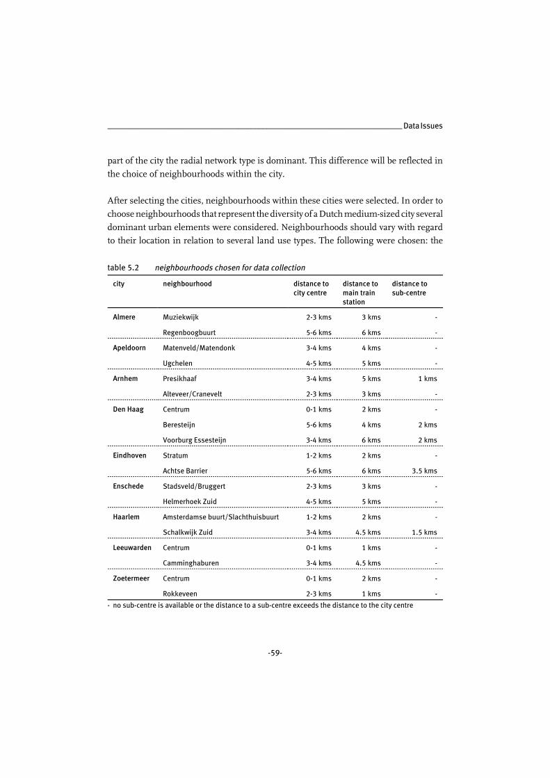
________________________________________________________________________ Data Issues
-59-
part of the city the radial network type is dominant. This difference will be reflected in
the choice of neighbourhoods within the city.
After selecting the cities, neighbourhoods within these cities were selected. In order to
choose neighbourhoods that represent the diversity of a Dutch medium-sized city several
dominant urban elements were considered. Neighbourhoods should vary with regard
to their location in relation to several land use types. The following were chosen: the
table 5.2 neighbourhoods chosen for data collection
city neighbourhood distance tocity centre
distance tomain trainstation
distance tosub-centre
Almere Muziekwijk 2-3 kms 3 kms -
Regenboogbuurt 5-6 kms 6 kms -
Apeldoorn Matenveld/Matendonk 3-4 kms 4 kms -
Ugchelen 4-5 kms 5 kms -
Arnhem Presikhaaf 3-4 kms 5 kms 1 kms
Alteveer/Cranevelt 2-3 kms 3 kms -
Den Haag Centrum 0-1 kms 2 kms -
Beresteijn 5-6 kms 4 kms 2 kms
Voorburg Essesteijn 3-4 kms 6 kms 2 kms
Eindhoven Stratum 1-2 kms 2 kms -
Achtse Barrier 5-6 kms 6 kms 3.5 kms
Enschede Stadsveld/Bruggert 2-3 kms 3 kms -
Helmerhoek Zuid 4-5 kms 5 kms -
Haarlem Amsterdamse buurt/Slachthuisbuurt 1-2 kms 2 kms -
Schalkwijk Zuid 3-4 kms 4.5 kms 1.5 kms
Leeuwarden Centrum 0-1 kms 1 kms -
Camminghaburen 3-4 kms 4.5 kms -
Zoetermeer Centrum 0-1 kms 2 kms -
Rokkeveen 2-3 kms 1 kms -
- no sub-centre is available or the distance to a sub-centre exceeds the distance to the city centre

Urban Form and Activity-Travel Patterns __________________________________________
-60-
location of the neighbourhood in relation to the city centre, to the main IC-train station
and, if present, to a sub-centre of services at the city district level. The city centre was
regarded as a focal point and neighbourhoods were selected in each city in 1 kilometre
wide rings from this centre. Per city, chosen neighbourhoods were dispersed over the
city. A list of 5 or 6 neighbourhoods per city was drawn up. The final choice was based
on the following considerations: 1) two neighbourhoods per city to obtain an even
distribution over the cities; 2) aggregated over all cities at least two neighbourhoods in
every ring from the city centre and 3) the best possible combinations with regard to the
other urban form characteristics. Ultimately, 19 neighbourhoods were chosen for data
collection (see table 5.2). Appendix 2 gives an overview of each city and neighbourhood
and their characteristics.
The characteristics of the chosen neighbourhoods were tested for mutual correlations,
to check if the chosen neighbourhoods actually allow us to better test the relationships
between characteristics of the urban environment and activity-travel patterns.
Correlations were calculated for 11 characteristics of urban form: urban shape, city road
network type, neighbourhood road network type, local street network type, employment
(number of jobs/businesses), location of city within the Netherlands (inside or outside
the Randstad Holland), distance from the neighbourhood to the city centre, distance
from the neighbourhood to the IC-station, distance from the neighbourhood to a sub-
centre of services and degree of urbanisation (neighbourhood and city). Definitions of
these characteristics are given in section 5.5.
Results are listed in table 5.3. Different association measures (Pearsons correlation
coefficient, symmetric lambda and eta coefficient) were used, depending on the type of
variables the association was calculated for. The results were quite satisfactory. Most
characteristics are not mutually associated. Only a few characteristics show correlations
that exceed a value of 0.5. Distance to city centre and to IC-station are highly correlated
(0.845). This can easily be explained by the fact that the main train station is usually (but
not always) located in the city centre. Furthermore, the distance to a sub-centre is
correlated with the network type neighbourhood ( = 0.857) and with the degree ofε 2urbanisation of the neighbourhood ( = 0.953). Finally, urban shape is related to theε 2city’s employment level ( = 0.766).ε 2

________________________________________________________________________ Data Issues
-61-
table 5.3 associations between neighbourhood characteristics (n=19)
netw.
type
city
netw.
type
nghbh
street
netw.
type
empl. location dist. to
city
centre
dist. to
ic-
station
dist. to
sub
centre
degree
of
urbanis.
neighbh
degree of
urbanis.
city
urban
form
ns ns ns = .77 ns = .06 = .06 = .06 =.39 =.43ε 2 ε 2 ε 2 ε 2 λ λ
network
type city
- =.42 ns = .07 ns = .12 = .17 = .06 ns =.48λ ε 2 ε 2 ε 2 ε 2 λ
network
type
neighbh
- - =.15 = .35 ns = .14 = .26 = .86 ns nsλ ε 2 ε 2 ε 2 ε 2
street
network
type
- - - = .43 ns = .48 = .44 = .10 =.38 nsε 2 ε 2 ε 2 ε 2 λ
empl. - - - - = .40 ns ns ns = .04 = .32ε 2 ε 2 ε 2
location - - - - - = .01 = .02 = .06 ns nsε 2 ε 2 ε 2
distance
to city
centre
- - - - - - 0.845 ns = .25 = .10ε 2 ε 2
distance
to ic-
station
- - - - - - - ns = .19 = .09ε 2 ε 2
distance
to
subcentre
- - - - - - - - = .95 = .06ε 2 ε 2
degree of
urbanis.
neighbh
- - - - - - - - - ns
degree of
urbanis.
city
- - - - - - - - - -
ns = not significant
5.3 Design of the Questionnaire
The activity diary questionnaire consisted of several parts, one of which was the actual
activity diary, the core of the questionnaire (figure 5.3). For each successive activity in a
two day period, respondents were asked to provide information about i) the kind of
activity, ii) the day, start and end time, iii) the location where the activity was conducted,
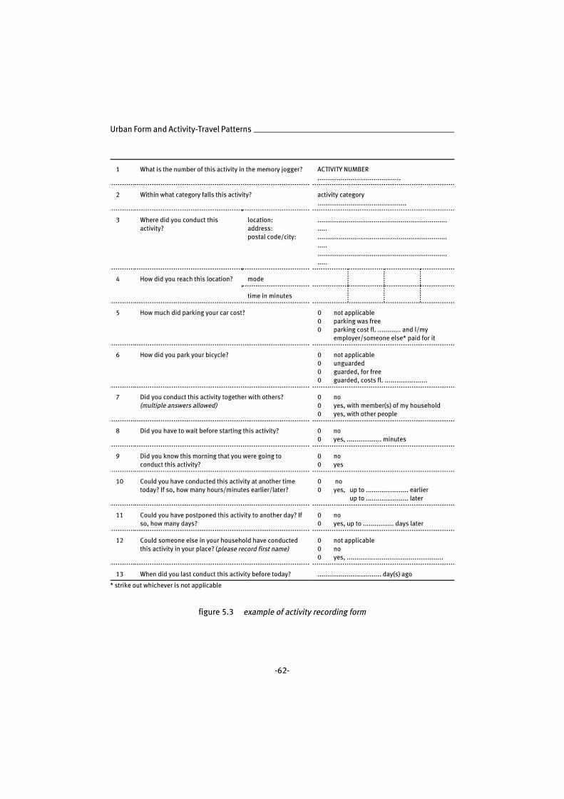
Urban Form and Activity-Travel Patterns __________________________________________
-62-
1 What is the number of this activity in the memory jogger? ACTIVITY NUMBER...........................................
2 Within what category falls this activity? activity category..............................................
3 Where did you conduct thisactivity?
location:address:postal code/city:
...................................................................
.....
...................................................................
.....
...................................................................
.....
4 How did you reach this location? mode
time in minutes
5 How much did parking your car cost? 0 not applicable0 parking was free0 parking cost fl. ............ and I/my
employer/someone else* paid for it
6 How did you park your bicycle? 0 not applicable0 unguarded0 guarded, for free0 guarded, costs fl. ......................
7 Did you conduct this activity together with others?(multiple answers allowed)
0 no0 yes, with member(s) of my household0 yes, with other people
8 Did you have to wait before starting this activity? 0 no0 yes, .................. minutes
9 Did you know this morning that you were going toconduct this activity?
0 no0 yes
10 Could you have conducted this activity at another timetoday? If so, how many hours/minutes earlier/later?
0 no0 yes, up to ...................... earlier
up to ...................... later
11 Could you have postponed this activity to another day? Ifso, how many days?
0 no0 yes, up to ................ days later
12 Could someone else in your household have conductedthis activity in your place? (please record first name)
0 not applicable0 no0 yes, ..................................................
13 When did you last conduct this activity before today? ................................. day(s) ago
* strike out whichever is not applicable
figure 5.3 example of activity recording form
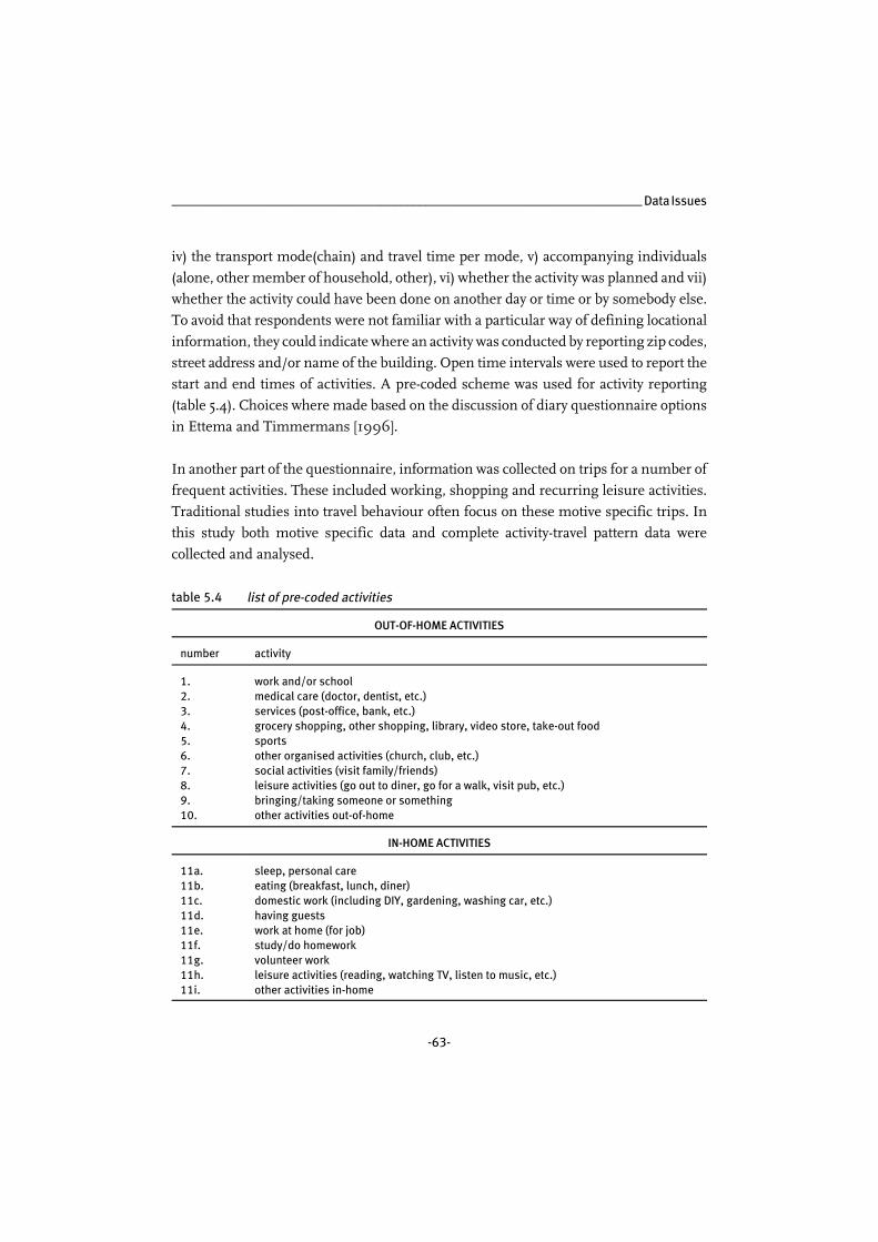
________________________________________________________________________ Data Issues
-63-
iv) the transport mode(chain) and travel time per mode, v) accompanying individuals
(alone, other member of household, other), vi) whether the activity was planned and vii)
whether the activity could have been done on another day or time or by somebody else.
To avoid that respondents were not familiar with a particular way of defining locational
information, they could indicate where an activity was conducted by reporting zip codes,
street address and/or name of the building. Open time intervals were used to report the
start and end times of activities. A pre-coded scheme was used for activity reporting
(table 5.4). Choices where made based on the discussion of diary questionnaire options
in Ettema and Timmermans [1996].
In another part of the questionnaire, information was collected on trips for a number of
frequent activities. These included working, shopping and recurring leisure activities.
Traditional studies into travel behaviour often focus on these motive specific trips. In
this study both motive specific data and complete activity-travel pattern data were
collected and analysed.
table 5.4 list of pre-coded activities
OUT-OF-HOME ACTIVITIES
number activity
1.2.3.4.5.6.7.8.9.10.
work and/or schoolmedical care (doctor, dentist, etc.)services (post-office, bank, etc.)grocery shopping, other shopping, library, video store, take-out foodsportsother organised activities (church, club, etc.)social activities (visit family/friends)leisure activities (go out to diner, go for a walk, visit pub, etc.)bringing/taking someone or somethingother activities out-of-home
IN-HOME ACTIVITIES
11a.11b.11c.11d.11e.11f.11g.11h.11i.
sleep, personal careeating (breakfast, lunch, diner)domestic work (including DIY, gardening, washing car, etc.)having guestswork at home (for job)study/do homeworkvolunteer workleisure activities (reading, watching TV, listen to music, etc.)other activities in-home

Urban Form and Activity-Travel Patterns __________________________________________
-64-
This way, differences between both approaches can be brought to light. For each of the
activities, respondents were asked to report when and where these activities are usually
performed, what the origin(s) of the trips to these locations is/are, which transportation
modes are used and what the travel time is.
The last part of the questionnaire focussed on various individual and household
characteristics. The information collected included year of birth, gender, level of
education, personal income, possession of a driver’s license, type of dwelling, and
availability of transport modes.
5.4 Response and Respondents
In each neighbourhood 300 randomly selected households received a letter requesting
their participation in the project. The letter explained the scope of the research project
and briefly described the task respondents had to perform. Households that responded
positively received a package containing as many questionnaires as there were
individuals aged 13 years and over in the household. The number of positive responses
to the letter requesting a households participation in the project varied widely across
neighbourhoods, resulting in different numbers of questionnaires being send out to
different neighbourhoods. 355 households returned 586 individual questionnaires.
5.4.1 Response Rates
Earlier it has been argued that diary data potentially yields a more detailed recording of
activities and related travel. However, the completion of diary questionnaires is rather
demanding and could therefore result in higher non-response rates. This section looks
at the response rates by geographical origin and by spatial and sociodemographic
characteristics.
The response rates for households for the 9 cities included in the data collection varied
between 47% and 78%, as shown in table 5.5. To test for any significant differences
between these response rates, a probit regression analysis using effect coding was
conducted. Dummy variables for each of the cities were used as independent variables.
The results indicate that the response rate was significantly lower in Almere and

________________________________________________________________________ Data Issues
-65-
table 5.5 response rates by city of those willing to participate after initial contact
city response rate city response rate
# % # %
Almere 30 46.9% Enschede 22 50.0%
Apeldoorn 61 68.5% Haarlem 27 62.8%
Arnhem 53 77.9% Leeuwarden 44 65.7%
Den Haag 41 51.3% Zoetermeer 29 52.7%
Eindhoven 48 57.1%
table 5.6 probit estimates of city characteristics (n=594)
variable estimate t-value
location -0.01263 -0.112
degree of urbanisation 0.05207 0.386
population size 0 -0.971
employment 0.00141 1.476
significantly higher in Arnhem (5% probability level). Another probit regression analysis
was performed to estimate the effect of location within the Netherlands (inside or
outside the Randstad Holland), the degree of urbanisation, population size and
employment of each city. These results are listed in table 5.6, and show that none of the
effects are statistically significant at the conventional level.
Response rates for the 19 neighbourhoods showed considerable more variation than for
the 9 cities (see table 5.7). The lowest percentage is 33.3%, whereas the highest
percentage is 80.4%. The results of the probit regression analysis using dummy
variables for each of the neighbourhoods indicated that exactly these two
neighbourhoods have response rates that differ significantly from the mean response
rates. In another probit analysis, the relationship between neighbourhood characteristics
and response rates was tested (table 5.8). In particular, the following variables were
included in the analysis: distance to city centre, land use mix and degree of urbanisation
of the neighbourhood. The latter variable proved to be significantly related to response
rate, in the sense that the response rate increases with decreasing density. For further
details on the analysis of the response rates, see Snellen et al, [2001].
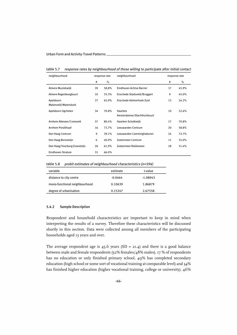
Urban Form and Activity-Travel Patterns __________________________________________
-66-
table 5.7 response rates by neighbourhood of those willing to participate after initial contact
neighbourhood response rate neighbourhood response rate
# % # %
Almere Muziekwijk 20 58.8% Eindhoven Achtse Barrier 17 45.9%
Almere Regenboogbuurt 10 33.3% Enschede Stadsveld/Bruggert 9 45.0%
Apeldoorn
Matenveld/Matendonk
27 65.9% Enschede Helmerhoek Zuid 13 54.2%
Apeldoorn Ugchelen 34 70.8% Haarlem
Amsterdamse/Slachthuisbuurt
10 52.6%
Arnhem Alteveer/Cranevelt 37 80.4% Haarlem Schalkwijk 17 70.8%
Arnhem Presikhaaf 16 72.7% Leeuwarden Centrum 20 58.8%
Den Haag Centrum 9 39.1% Leeuwarden Camminghaburen 24 72.7%
Den Haag Beresteijn 6 40.0% Zoetermeer Centrum 11 55.0%
Den Haag/Voorburg Essesteijn 26 61.9% Zoetermeer Rokkeveen 18 51.4%
Eindhoven Stratum 31 66.0%
table 5.8 probit estimates of neighbourhood characteristics (n=594)
variable estimate t-value
distance to city centre -0.0464 -1.08943
mono-functional neighbourhood 0.10639 1.86879
degree of urbanisation 0.15247 2.67558
5.4.2 Sample Description
Respondent and household characteristics are important to keep in mind when
interpreting the results of a survey. Therefore these characteristics will be discussed
shortly in this section. Data were collected among all members of the participating
households aged 13 years and over.
The average respondent age is 45.6 years (SD = 21.4) and there is a good balance
between male and female respondents (52% females/48% males). 17 % of respondents
has no education or only finished primary school, 49% has completed secondary
education (high school or some sort of vocational training at comparable level) and 34%
has finished higher education (higher vocational training, college or university). 46%

________________________________________________________________________ Data Issues
-67-
of respondents work full time and 16% work part time, others are not engaged in (paid)
work activities. 48% of respondents have personal net income of 30.000,- Dutch
guilders or less per year, while 27% earn more than 50.000,- Dutch guilders annually.
94% of respondents have one or more bicycles available. 78% of respondents have a
driver’s license, 49% of respondents have a car directly available, while another 26%
have a car available which they share with someone else (within or outside the
household). Finally, 37% of respondents have some kind of public transport pass. This
figures includes people owning a railway discount card (voordeelurenkaart) and senior
citizens that have a pass that entitles them to bus travel at reduced prices.
From the questionnaire a number of household characteristics were available. 28% of
households are single person households, 38% are couples and 32% are families with
children. Overall, 68% of households do not have children, 17% have children under 12
years old and 16% have older children. When engagement in work by household
members is included in the household typology, we found that 30% of households are
dual earner households.
Household income was calculated from the personal incomes of household members
and divided into 4 categories. Little over half of responding households have an income
of 2 times standard and over, while 21% is below standard, 10% is approximately
standard and 18% is between 1 and 2 times standard. The housing situation of
responding households was also considered. 25% of households live in a flat or
apartment, 54% in a terraced single family house and 21% in a (semi)detached single
family house. 61% of households own their house, while 39% rents. 78% of households
have a garden, while 19% has a balcony and only 3% does not have outdoor space of any
kind. Average number of bedrooms is 3.1 (SD = 1.2). 87% of households owning a car,
park this car in the direct vicinity of the house (on driveway, in garage near their house,
on the street in front of the house or apartment building, etcetera).
Finally, since the ability to test the relationship between the characteristics of the urban
environment and activity and travel patterns could be negatively influenced by strong
relations between socioeconomic characteristics of respondents and characteristics of
neighbourhoods, we tested for correlations between them. Correlations were calculated
between nine socioeconomic characteristics of respondents and households (viz.
household composition, household income, dwelling type, gender, age, education level,

Urban Form and Activity-Travel Patterns __________________________________________
-68-
personal income, work status and availability of motorised transport) and the
characteristics of the urban environment. The results are shown in table 5.9. No
correlations exceeding 0.500 were found. In fact, most significant associations were
lower that 0.05, which is a very satisfactory result.
table 5.9 associations between neighbourhood characteristics and socioeconomic
characteristics (n=594)
netw.
type
city
netw.
type
nghbh
street
netw.
type
empl. loca
tion
dist. to
city
centre
dist. to
ic-
station
dist. to
sub
centre
degree
urbanis
nghbh
degree
urbanisc
ity
age = .01 = .02 = .04 ns = .00 ns 0.105 ns = .06 = .00ε 2 ε 2 ε 2 ε 2 ε 2 ε 2
hh.comp. =.04 ns ns = .08 ns = .05 = .03 = .08 ns nsλ ε 2 ε 2 ε 2 ε 2
hh.income =.04 ns ns = .03 ns = .01 = .02 = .05 ns nsλ ε 2 ε 2 ε 2 ε 2
dwelling
type
=.08 ns =.11 = .03 ns = .09 = .05 = .06 =.10 nsλ λ ε 2 ε 2 ε 2 ε 2 λ
gender ns ns ns = .00 ns = .00 = .00 = .01 ns nsε 2 ε 2 ε 2 ε 2
education
level
ns ns ns = .00 ns = .03 = .02 = .04 ns nsε 2 ε 2 ε 2 ε 2
personal
income
ns ns =.04 = .01 ns = .01 = .01 = .03 ns nsλ ε 2 ε 2 ε 2 ε 2
work.
status
ns ns ns = .01 ns = .02 = .01 = .02 ns nsε 2 ε 2 ε 2 ε 2
car
ownership
ns ns ns = .01 ns = .02 = .02 = .06 ns nsε 2 ε 2 ε 2 ε 2
ns = not significant
5.4.3 Data Quality
In their discussion of errors in activity diaries, Arentze and Timmermans [2000]
mention that this type of questionnaire is more prone to errors and inconsistencies than
other travel surveys. Most common errors are caused by skipping transfer activities
(sequence of activity and/or place from outdoors to indoors and vice versa). Other
common errors are the result of missing information about other people, about the
timing of activities and inconsistencies between activity and place. The data collected for
this study was examined to establish whether inconsistencies and errors in the activity
diaries were related to the geographical origin of the respondents and/or a number of
their socioeconomic characteristics.
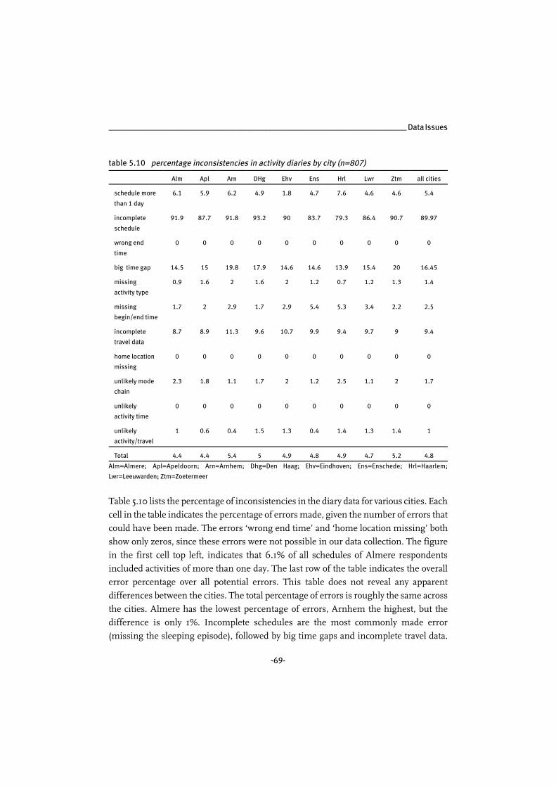
________________________________________________________________________ Data Issues
-69-
table 5.10 percentage inconsistencies in activity diaries by city (n=807)
Alm Apl Arn DHg Ehv Ens Hrl Lwr Ztm all cities
schedule more
than 1 day
6.1 5.9 6.2 4.9 1.8 4.7 7.6 4.6 4.6 5.4
incomplete
schedule
91.9 87.7 91.8 93.2 90 83.7 79.3 86.4 90.7 89.97
wrong end
time
0 0 0 0 0 0 0 0 0 0
big time gap 14.5 15 19.8 17.9 14.6 14.6 13.9 15.4 20 16.45
missing
activity type
0.9 1.6 2 1.6 2 1.2 0.7 1.2 1.3 1.4
missing
begin/end time
1.7 2 2.9 1.7 2.9 5.4 5.3 3.4 2.2 2.5
incomplete
travel data
8.7 8.9 11.3 9.6 10.7 9.9 9.4 9.7 9 9.4
home location
missing
0 0 0 0 0 0 0 0 0 0
unlikely mode
chain
2.3 1.8 1.1 1.7 2 1.2 2.5 1.1 2 1.7
unlikely
activity time
0 0 0 0 0 0 0 0 0 0
unlikely
activity/travel
1 0.6 0.4 1.5 1.3 0.4 1.4 1.3 1.4 1
Total 4.4 4.4 5.4 5 4.9 4.8 4.9 4.7 5.2 4.8
Alm=Almere; Apl=Apeldoorn; Arn=Arnhem; Dhg=Den Haag; Ehv=Eindhoven; Ens=Enschede; Hrl=Haarlem;
Lwr=Leeuwarden; Ztm=Zoetermeer
Table 5.10 lists the percentage of inconsistencies in the diary data for various cities. Each
cell in the table indicates the percentage of errors made, given the number of errors that
could have been made. The errors ‘wrong end time’ and ‘home location missing’ both
show only zeros, since these errors were not possible in our data collection. The figure
in the first cell top left, indicates that 6.1% of all schedules of Almere respondents
included activities of more than one day. The last row of the table indicates the overall
error percentage over all potential errors. This table does not reveal any apparent
differences between the cities. The total percentage of errors is roughly the same across
the cities. Almere has the lowest percentage of errors, Arnhem the highest, but the
difference is only 1%. Incomplete schedules are the most commonly made error
(missing the sleeping episode), followed by big time gaps and incomplete travel data.

Urban Form and Activity-Travel Patterns __________________________________________
-70-
The other types of errors occur considerably less. In tables 5.11a and b, the attention
shifts to the neighbourhood level. The range in the percentage of errors increases, as is
to be expected. However, overall differences are still small. The rank order of most
commonly made errors is the same as observed for the city level. Incomplete schedules,
big time gaps and incomplete travel data are the most commonly made errors.
table 5.11a inconsistencies in activity diaries by neighbourhood (n=807)
Almere Apeldoorn Arnhem Den Haag
Mzw Rgb Mvd Ugc A/C Prh Ctr Bsn VEs
schedule more
than 1 day
7.5 0 2.6 9.5 12.5 3 0 16.7 3.1
incomplete
schedule
91 93.9 82.9 91.6 95.3 84.9 90 94.4 96.9
wrong end time 0 0 0 0 0 0 0 0 0
big time gap 17.2 9.7 14.4 15.2 21.4 15.3 18.8 23.9 16.4
missing activity
type
0.9 0.9 2 1.3 1.2 3.1 0.8 2.5 1.2
missing
begin/end time
1 3.1 2.4 1.8 2 5.1 2.3 2.3 1.3
incomplete
travel data
8.8 8.4 6.8 10.7 11.4 13 11.9 11.3 9.2
home location
missing
0 0 0 0 0 0 0 0 0
unlikely mode
chain
1.9 2.6 1.7 1.8 1.3 1.3 2.5 0.4 1.8
unlikely activity
time
0 0 0 0 0 0 0 0 0
unlikely
activity/travel
1 0.2 0.9 0.3 0.4 0.5 0.8 1.3 1.8
Total 4.6 3.9 4.2 4.6 5.5 5.4 5.3 5.9 4.7
Mzw=Muziekwijk; Rgb=Regenboogbuurt; Mvd=Matenveld/donk; Ugc=Ugchelen; A/C=Alteveer/Cranevelt; Prh=Presikhaaf;
Ctr=Centrum; Bsn=Beresteijn; Ves=Voorburg Essesteijn
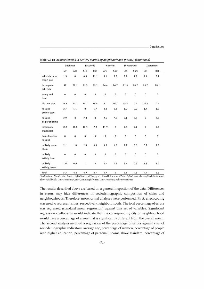
________________________________________________________________________ Data Issues
-71-
table 5.11b inconsistencies in activity diaries by neighbourhood (n=807) (continued)
Eindhoven Enschede Haarlem Leeuwarden Zoetermeer
Str Abr S/B Hlm A/S Skw Cnt Cam Cnt Rok
schedule more
than 1 day
1.5 0 6.3 11.1 9.1 3.3 2.9 1.9 4.4 7.1
incomplete
schedule
97 79.1 81.3 85.2 86.4 76.7 82.9 88.7 95.7 88.1
wrong end
time
0 0 0 0 0 0 0 0 0 0
big time gap 16.6 11.2 10.1 18.4 11 16.7 15.8 15 16.4 22
missing
activity type
2.7 1.1 0 1.7 0.8 0.3 1.9 0.9 1.4 1.2
missing
begin/end time
2.9 3 7.8 3 2.5 7.6 5.1 2.5 2 2.3
incomplete
travel data
10.1 10.8 12.3 7.9 11.9 8 9.3 9.4 9 9.2
home location
missing
0 0 0 0 0 0 0 0 0 0
unlikely mode
chain
2.1 1.8 2.6 0.3 3.5 1.6 2.2 0.6 0.7 2.3
unlikely
activity time
0 0 0 0 0 0 0 0 0 0
unlikely
activity/travel
1.6 0.9 1 0 2.7 0.3 2.7 0.6 1.8 1.4
Total 5.3 4.2 4.9 4.7 4.9 5 5.3 4.3 4.7 5.5Str=Stratum; Abr=Achtse Barrier; S/B=Stadsveld/Bruggert; Hlm=Helmerhoek Zuid; A/S=Amsterdamse/Slachthuisbuurt;
Skw=Schalkwijk; Cnt=Centrum; Cam=Camminghaburen; Cnt=Centrum; Rok=Rokkenveen
The results described above are based on a general inspection of the data. Differences
in errors may hide differences in sociodemographic composition of cities and
neighbourhoods. Therefore, more formal analyses were performed. First, effect coding
was used to represent cities, respectively neighbourhoods. The total percentage of errors
was regressed (standard linear regression) against this set of variables. Significant
regression coefficients would indicate that the corresponding city or neighbourhood
would have a percentage of errors that is significantly different from the overall mean.
The second analysis involved a regression of the percentage of errors against a set of
sociodemographic indicators: average age, percentage of women, percentage of people
with higher education, percentage of personal income above standard, percentage of

Urban Form and Activity-Travel Patterns __________________________________________
-72-
household income above standard, percentage of people with a driver’s license,
percentage of car ownership, percentage of singles, percentage of single family dwellings
and percentage of unemployed. Tables 5.12 and 5.13 report the results of these
regressions at the city level. From the tables one can see that neither the indicator
variables for the cities, nor the coefficients of the city characteristics are significant at the
conventional probability level. Thus, the percentage of errors in the activity diaries does
table 5.12 regression of errors by city (n=9)
unstandardised coefficients
B Std. Error t-value Sig.
(Constant) 9.764 0.316 30.899 0
Almere -0.282 0.822 -0.343 0.732
Apeldoorn 0.001 0.655 0.017 0.986
Arnhem 1.019 0.798 1.277 0.202
Den Haag 1.046 0.81 1.292 0.197
Eindhoven 0.469 0.798 0.588 0.557
Enschede -1.687 1.157 -1.458 0.147
Haarlem -0.971 1.101 -0.882 0.378
Leeuwarden 0.159 0.848 0.187 0.852
table 5.13 regression of errors by socioeconomic indicators city (n=9)
unstandardised coefficients
B Std.Error t-value Sig.
(Constant) 8.551 18.113 0.472 0.637
average age -0.008 0.161 -0.519 0.604
% of women -0.406 0.33 -1.23 0.219
% of people with higher education 0.569 0.38 1.497 0.135
% of personal income above standard -0.191 0.179 -1.067 0.287
% of household income above standard -0.008 0.152 -0.56 0.575
% of people with a driver’s license -0.009 0.151 -0.562 0.575
% car ownership 0.005 0.058 0.838 0.402
% of singles 0.309 0.192 1.613 0.107

________________________________________________________________________ Data Issues
-73-
not vary more than randomly across the cities nor across the urban indicators. Model
performance is low (R-square=0.012) in both cases.
A similar analysis was conducted at the neighbourhood level. The standard regression
model performed equally bad with a R-square of 0.02. The results are reported in tables
5.14 and 5.15. Table 5.14 shows that the percentage of errors does not differ significantly
from the overall mean in any of the neighbourhoods, which means that there are no
significant spatial effects at this level of aggregation. Table 5.15 reports the estimated
coefficients for the case where the neighbourhoods have been classified according to a
table 5.14 regression of errors by neighbourhoods (n=19)
unstandardised coefficients
B Std.Error t-value Sig.
(Constant) 9.816 0.338 29.05 0
Almere Muziekwijk -0.007 1.037 -0.07 0.945
Almere Regenboogbuurt -0.933 1.523 -0.613 0.540
Apeldoorn Matenveld/Matendonk -1.411 1.004 -1.406 0.160
Apeldoorn Ugchelen 0.988 0.885 1.116 0.265
Arnhem Alteveer/Cranevelt 0.77 1.014 0.759 0.448
Arnhem Presikhaaf 1.395 1.445 0.965 0.335
Den Haag Centrum 1.184 1.877 0.631 0.528
Den Haag Beresteijn 1.549 1.877 0.825 0.410
Den Haag/Voorburg Essesteijn 0.768 1.078 0.714 0.476
Eindhoven Stratum 0.441 1.089 0.405 0.685
Eindhoven Achtse Barrier 0.384 1.271 0.302 0.762
Enschede Stadsveld/Bruggert -1.482 2.069 -0.716 0.474
Enschede Helmerhoek Zuid -1.875 1.523 -1.231 0.219
Haarlem Amsterdamse/Slachthuisbuurt -0.149 1.8 -0.083 0.934
Haarlem Schalkwijk -1.639 1.523 -1.076 0.282
Leeuwarden Centrum -0.216 1.411 -0.153 0.879
Leeuwarden Camminghaburen 0.309 1.134 0.273 0.785
Zoetermeer Centrum -0.601 1.671 -0.36 0.719

Urban Form and Activity-Travel Patterns __________________________________________
-74-
table 5.15 regression of errors by socioeconomic indicators neighbourhood (n=19)
unstandardised coefficients
B Std.Error t-value Sig.
(Constant) 0.965 6.555 0.147 0.883
average age 0.004 0.101 0.404 0.687
% of women 0.006 0.057 1.041 0.298
% of people with higher education 0.003 0.031 0.91 0.363
% of personal income above standard 0 0.065 0.071 0.943
% of household income above standard 0.002 0.057 0.332 0.740
% of people with a driver’s license -0.146 0.109 -1.341 0.181
% car ownership 0.2 0.116 1.727 0.085
% of singles 0 0.064 0.08 0.936
% of single dwellings -0.003 0.028 -0.973 0.331
% unemployed -0.001 0.052 -0.227 0.820
set of aggregate neighbourhood characteristics. None of the effects is statistically
significant at the conventional 5% probability level.
The analysis described above has relied on socioeconomic variables that were aggregated
from individual level data. It implies that we cannot control for individual variation in
errors. Moreover, this aggregation results in fewer values for less units of observation,
implying that the power of the statistical analysis is reduced. To further explore whether
the results may be an artifact of these operational decisions, a multilevel analysis was
conducted. This type of analysis, also known as hierarchical linear modelling, was
introduced in the previous chapter. More detailed information on model estimation and
model performance assessment can be found in chapter 6.
Table 5.16 reports the results of the multilevel analysis. The two levels in the analysis are
the individual and the neighbourhood. The results show that the number of errors
increases with age and decreases with income. Although these variables are significant
(age at the 5% level and income at the 10% level), their explanatory power is very limited
(only 1,2%). Important however for the present study is that the estimated effects for

________________________________________________________________________ Data Issues
-75-
variables describing cities and neighbourhoods are not significant, giving further
support to the results obtained with the less advanced methods of analysis.
table 5.16 multi level analysis of diary inconsistencies (n=370 respondents)
Estimated effect (standard error)
fixed part
individual effects
intercept
age
income standard and over
random part:
individual
group (neighbourhood)
7.886 (1.082)
0.046 (0.022)
-0.655 (0.355)
43.733
0.024
individualR2groupR2
0.012
0.000
5.4.4 Conclusions
In the previous sections, the response rates, the quality of the data and the characteristics
of the respondents have been looked at in detail. Results are satisfying. No high
correlations were found between characteristics of the individual respondents and
responding households and the urban environment they come from. Response rates are
rather independent of spatial characteristics. Some significant differences were found.
Response rates for the cities of Almere (lower) and Arnhem (higher), and, within these
cities, for the neighbourhoods Muziekwijk (lower) and Alteveer/Cranevelt (higher),
differ significantly from the overall mean. Furthermore it was found that
neighbourhoods with lower densities have slightly higher response rates.
Finally, we looked at the quality of the data by urban form and sociodemographic
characteristics. The number of errors in the diaries was regressed against a set of
indicators. No significant differences between cities or neighbourhoods were found, nor
any significant effects of spatial or sociodemographic descriptors. A more sophisticated
analysis, using multilevel modelling, revealed some significant effects of age and
income, however, the explanatory power of this model was rather limited.

Urban Form and Activity-Travel Patterns __________________________________________
-76-
It can therefore be concluded that there is little bias in the data. Some influence of
socioeconomic factors was found, but this was as expected. Hardly any evidence of
spatial bias was found. This is a positive result in the sense that no further weighting
schemes are required for subsequent analyses.
5.5 Independent Variables
Three groups of variables play an important role in this research project. The first group
comprises the dependent variables describing the activity and travel patterns of people.
These variables can be derived from the data collection and are described in further
detail in chapters 6 and 7. The other two groups are independent variables describing
i) the spatial context of the city and neighbourhood and ii) the socioeconomic
characteristics of the respondents. These two groups of independent variables are
discussed and defined in this section.
5.5.1 Variables Describing the Spatial Context
In the chapters 2 and 3, policy documents and (scientific) literature were studied in order
to assess which elements of urban form are expected to yield positive or negative effects
when mobility reduction is pursued. In general, policy and literature do not differ all that
much. Both work with the same basic principles to achieve mobility (growth) reduction:
shorter distances and a shift in mode choice towards non-motorised and public
transport. Similar measures and urban design principles are considered to yield positive
effects. The most important are concentrated, centralised urban development, mixed
land use, high density development, location policy (the right activity at the right place),
good public transport, good walking/cycling facilities and an urban design that
discourages car use.
The first three items are clearly urban form characteristics and can be operationalised
rather straightforward. The items that follow, which focus more on the available
transport system, are more complicated. The term ‘good’ is not easy to interpret or
operationalise. Especially with regard to public transport, studies and policy documents
tend to operationalise ‘good’ mainly in terms of transport service provision, e.g. high
frequency, high quality of vehicles, use of rail systems. Rarely, urban design or form
elements are associated with ‘good’ public transport. In contrast, ‘good’ walking and

________________________________________________________________________ Data Issues
-77-
cycling facilities are more often operationalised in urban form or design characteristics.
The literature on The New Urbanism offers several examples of this [CNU, 2000a;
CNU, 2000b]. Availability of sidewalks and cyclepaths, separate cycle networks and grid
type transportation networks are some of the design elements associated with ‘good’
facilities. The last item, urban design that discourages car use, is also sparsely
operationalised. Usually this is related to facilities for transportation alternatives and to
the availability of activity locations within reach of non-motorised and public transport.
The specific contribution of different types of transportation networks is subject of study
in the literature on neo-traditional development and New Urbanism. Empirical studies
focussing on the effects of these types of development do look at transportation
networks, however, a limited set of network types is usually studied (e.g. Friedman et al
[1994], Nasar [1997], Florez [1998], Cervero [1996] and Cervero and Gorham [1995]).
The urban form elements that will be studied in this thesis are partly derived from policy
and literature and partly form an extension to what has been studied previously. The
elements are classified in three main categories. The first category includes the basic
urban shape and transportation networks in the urban environment. Although these
elements of urban form received relatively little attention in the studies discussed in
chapter 3, effects can be expected. Based on the theories with regard to the New
Urbanism and neo-traditional development, and the empirical studies in this tradition,
it appears to be an interesting path to follow. The second category focusses on relative
location of the neighbourhood with regard to different types of land use and land use
mix. It looks at different types of facilities available in the neighbourhood and the
distance to important other activity centres. Finally, the last category focusses at density.
In the preparatory steps of this study, a larger set of variables describing the spatial
environment was considered for inclusion. Some of the variables were deleted from the
list. Distance to a city district shopping centre and distance to a secondary train station were
deleted because these distances were only considered relevant if they were shorter than
the distances to the city centre and the main train station. Only for a subset of
neighbourhoods this was the case. Given the relatively small sample size, inclusion of
these variables was considered not effective. The variables describing the coverage of a
neighbourhood by the local bus service and the distance to the nearest motorway approach
were also deleted form the list because these variables showed very little variation over
the neighbourhoods.

Urban Form and Activity-Travel Patterns __________________________________________
-78-
figure 5.4 urban shapes
figure 5.5 transportation networks city
Below, each of the three categories of spatial variables will be operationalised by a
number of variables and their definition. Some of these variables have already been
defined in the previous section regarding the choice of locations for data collection. The
variable urban shape describes the basic morphological form of the city in question. The
levels of this variable (see figure 5.4) are ‘concentric’, ‘poly-nuclear’, ‘lobe’ and ‘grid’ and
are therefore the same as employed in the selection of cities for data collection (section
5.2.2).
The variable transportation network type city describes the basic transportation network
type that can be discerned for the city as a whole. Again this is the same variable as
employed for the selection of cities for data collection (section 5.2.3) and the levels used
are ‘radial’, ‘ring’ and ‘grid’ (figure 5.5). The grey area in the diagrams depicts the built
up area of the city.
The variable transportation network type neighbourhood describes the basic transportation
network type that can be discerned for the neighbourhood as a whole. The network types
were assessed based on neighbourhood maps and 6 different types were discerned
(figure 5.6). The grey area in the diagrams depicts the neighbourhood.

________________________________________________________________________ Data Issues
-79-
figure 5.6 transportation networks neighbourhood
figure 5.7 local street network types
The variable local street network type refers to the network type that can be discerned
within a neighbourhood on street level. This low level gives an indication of the network
type in the immediate proximity of the dwellings. Five network types, some of which are
composites, are discerned (see figure 5.7). Levels were assessed based on neighbourhood
maps. The grey area in the diagrams depicts the immediate surroundings of a local
street.
The variable location of the city within the country refers to
whether or not the city in question is located inside or
outside the Randstad Holland, the western, most
urbanised area of the Netherlands (see figure 5.8).
figure 5.8 location of the Randstad Holland
The variable employment city is defined as the number of jobs in the city per 1,000
inhabitants. It gives an indication of the jobs/population balance and therefore the towns
ability to be self contained. For some of the analyses this continuous variable is
Urban Form and Activity-Travel Patterns __________________________________________
-80-
converted into an ordinal variable with three categories: ‘low’ (less than 300 jobs per
1,000 inhabitants), ‘average’ (between 300 and 500 jobs per 1,000 inhabitants) and
‘high’ (more than 500 jobs per 1,000 inhabitants). National average is 388 jobs/1,000
inhabitants. Data was obtained from Statistics Netherlands.
Land use mix neighbourhood describes the measure to which the land use in the
neighbourhood is mixed. Mono-functional neighbourhoods (residential with few
facilities for the local population such as a small shopping centre) are defined as not
mixed. Neighbourhoods that include industrial and/or office functions, or that have
ample shopping facilities (such as neighbourhoods with a city district shopping centre)
are defined as mixed. Mixing was assessed based on neighbourhood maps and data on
businesses and shops (yellow pages).
Distance to the city centre describes the distance from the neighbourhood to the city
centre. It is the same variable as was used for the choice of neighbourhoods. Distance to
inter-city station simply describes the distance from the centre of the neighbourhood to
the nearest inter-city train station.
The variable locally available shopping facilities, describes the locally available shopping
facilities in the neighbourhood in 5 levels. Neighbourhoods are classified based on the
highest level shopping facility available in the neighbourhood. The levels discerned are
described below. Classification was made based on neighbourhood maps and data from
the yellow pages. The first category is ‘none or just a few local shops’, for example a
single bakery or butcher’s, florist or tobacconist. The second category is the ‘small
neighbourhood shopping centre’ consisting of a supermarket and possibly several
supporting shops such as a discount food market, some specialist food stores (bakery,
butcher’s, greengrocer’s, etcetera), some daily non food stores (drugstore, tobacconist,
florist, etcetera) and some services (bank or post-office, hairdresser’s, cafeteria, etcetera).
The ‘large neighbourhood shopping centre’ consists of 2 or more supermarkets and a
wide selection of the following: a complete supply of specialist food stores, several non-
food shops (also including shops for household goods and textiles, household appliances,
books, etcetera), several services, limited supply of clothing and shoes. The fourth
category is the ‘city district shopping centre’, consisting of a wide range of food stores
and supermarkets, a wide range of non-food shops and services, ample supply of fashion
and shoe stores catering for several target groups, a department store and supporting
facilities such as cafeteria’s, a restaurant and/or a leisure facility. Finally, the ‘city centre’

________________________________________________________________________ Data Issues
-81-
consists of a large number of shops in all categories, at least two department stores, and
all sorts of supporting facilities, food supply is often limited and concentrated in streets
of the main shopping street
The variable locally available sports facilities describes whether or not a neighbourhood
has sports facilities, such as a tennis court, a soccer field, a sports park and/or an indoor
sports centre locally available. Classification was made based on neighbourhood maps.
Three variables describe in different ways the density of the city as a whole. These are
housing density city, population density city and degree of urbanisation city. The housing
and population density simply describe the number of dwellings and inhabitants per
hectare surface area of the city. For some of the analyses these densities were
categorised. Population density has the following categories: ‘low’ ( 10≤inhabitants/hectare), ‘moderate’ (10-30 inhabitants/hectare), ‘fairly high’ (30-50
inhabitants/hectare) and ‘high’ (> 50 inhabitants/hectare). Housing density also has four
categories: ‘low’ ( 4 dwellings/hectare), ‘moderate’ (4-10 dwellings/hectare), ‘fairly≤high’ (10-30 dwellings/hectare) and ‘high’ (> 30 dwellings/hectare). Data was obtained
from Statistics Netherlands and the municipalities in question. The degree of
urbanisation is a measure based on the ‘surrounding address density’. This is the
average number of addresses per square kilometre within a 1 kilometre radius. For each
address in the city the individual surrounding address density is calculated and then the
average across all addresses is obtained. Based on this density measure, 5 degrees of
urbanisation were identified: ‘very strongly urbanised’ (surrounding address density of
2500 and over), ‘strongly urbanised’ (surrounding address density between 1500 and
2500), ‘moderately urbanised’ (surrounding address density between 1000 and 1500),
‘little urbanised’ (surrounding address density between 500 and 1000) and ‘not
urbanised’ (surrounding address density below 500). Data was obtained from Statistics
Netherlands.
Another three variables describe the density of the neighbourhood. These are housing
density neighbourhood, population density neighbourhood and degree of urbanisation
neighbourhood. The housing and population density simply describe the number of
dwellings and inhabitants per hectare surface area of the neighbourhood. For some of
the analyses these densities were categorised. Population density has the following
categories: ‘low’ (20-40 inhabitants/hectare), ‘moderate’ (40-60 inhabitants/hectare),
‘fairly high’ (60-80 inhabitants/hectare) and ‘high’ (>80 inhabitants/hectare). Housing

Urban Form and Activity-Travel Patterns __________________________________________
-82-
density also has four categories: ‘low’ ( 10 dwellings/hectare), ‘moderate’ (10-20≤dwellings/hectare), ‘fairly high’ (20-30 dwellings/hectare) and ‘high’ (> 30
dwellings/hectare). The degree of urbanisation of a neighbourhood is defined similar
to the degree of urbanisation of the city, as described above. Data was obtained from
Statistics Netherlands and the municipalities in question.
5.5.2 Socioeconomic Variables
The last group of variables relevant for the analysis of the relationship between urban
form and travel patterns are the socioeconomic control variables describing individual
and household characteristics. All of these data were obtained from the questionnaires.
The socioeconomic data include the following individual characteristics: age, gender,
education level, personal income, possession of a driver’s license and employment
status. Additionally, a number of household characteristics was included: car availability,
household income, socioeconomic class, household type, dwelling type and average
distance to chosen location. Characteristics were selected based on the prevalence of
variables in the literature. Appendix 3 gives and overview of definitions and
classifications for each of these variables.
Some characteristics initially selected were not included in the final analysis. Possession
of a public transport pass was not included. There were some concerns about the nature
of this variable. If people decide to choose public transport, then they will see whether
some kind of pass is in their interest. Hence, inclusion of this variable is likely to
confound the effect of truly ‘causal’ variables such as distance and frequency. Although
this could also be the case for car ownership, we feel that the decision to buy a car is
based on many more considerations than the decision to get a public transport pass.
Furthermore, possession of a bicycle and participation in a car sharing plan were not
included because of lack of variation. 94% of respondents owns one or more bicycles
and only 1% of respondents participated in a car sharing plan. Housing tenure was not
included as a separate variable because of its overlap with household income and
dwelling type. Finally, having a garden and/or balcony was not included because this is
largely covered by dwelling type and only 2% of respondents have neither one.
________________________________________________________________________ Data Issues
-83-
5.6 Summary and Conclusions
This chapter described the data collection process followed for this study. It discussed
the selection of locations based on a number of dominant urban form characteristics:
urban shape, main transportation network type, location in relation to the city centre and
main urban functions. It also discussed the design of the activity diary questionnaire.
The response that was the result of the data collection was discussed and analysed, both
with regard to the response rates and the quality of the response. Finally, the
independent variables that will be used in data analysis were discussed and defined.
It was found that, although the positive responses to our request to participate in the
research varied widely over neighbourhoods, both the response of those that received a
questionnaire, and the quality of the response are satisfying. Response rates proved, to
a large extent, to be independent of spatial characteristics. The quality of the data proved
not to be associated with spatial characteristics. Associations were found with age and
income. However, the explanatory power of this model was very limited. Overall, it can
be concluded that there is little bias in the data, especially with regard to spatial
characteristics. Most importantly, the methodological principle that socioeconomic and
sociodemographic characteristics should be as independent as possible from urban form
characteristics was realised.

-84-
6 | TRAVEL FOR FREQUENT ACTIVITIES
6.1 Introduction
A limited set of recurring, frequent activities takes up a large part of the total number
of trips and the total number of kilometres travelled by individuals and households. This
makes it interesting to see if, and how, these trips are influenced by spatial and
socioeconomic variables. This chapter will discuss the results for four types of trips for
recurring frequent activities, viz. home-to-work trips, grocery shopping trips, non-
grocery shopping trips and recurring leisure trips (such as regular trips to sports and
club activities). In 1998 these activities accounted for 50 percent of all trips and 49
percent of all kilometres [CBS, 1999]. Although we have argued that an analysis by
motive may lead to an incomplete assessment, we decided to conduct such an analysis
anyhow because it allows us to actually compare an analysis by motive and an analysis
of complete activity-travel patterns. The results of the latter analysis are reported in
chapter 7.
The relationship between urban form, socioeconomic variables and travel characteristics
will be analysed using multilevel analysis. As argued in chapter 4, this methodology
allows us to account for the fact that the independent variables (spatial and
socioeconomic) are measured at different levels of aggregation.
This chapter is organised as follows. In section 6.2 a general description of the travel
data on frequently made trips is given. Section 6.3 elaborates the basic discussion of the
multilevel model as presented in chapter 4. The results of the multilevel analyses are
discussed in section 6.4. In section 6.5 conclusions will be drawn.
_______________________________________________________ Travel for Frequent Activities
-85-
6.2 General Description of the Data
Our data on frequently made trips included trips originating from home with the
purpose of grocery shopping, non-grocery shopping, recurring leisure and work. Data
on grocery shopping trips was provided by 392 respondents, on non-grocery shopping
trips by 460 respondents, on recurring leisure trips by 340 respondents and on home-to-
work trips by 200 respondents. The following characteristics of travel behaviour were
obtained from the data: i) the total numbers of kilometres and trips, ii) the number of
kilometres and trips per mode and iii) mode shares for both kilometres and trips. The
numbers of kilometres travelled are based on straight line calculations of trip distances.
The time span for the dependent variables differed by travel motive. Grocery shopping
trips, recurring leisure trips and home-to-work trips were measured per month, non-
grocery shopping trips were measured per year. Motorised travel, non-motorised travel
and travel by public transport are discerned as transport modes in this study. Motorised
travel comprises travel by private car and by motorcycle. Non-motorised travel comprises
walking, cycling and travelling by moped. Public transport travel comprises all sorts of
public transport, such as travel by bus, by tram, by metro and by train. The data for
grocery shopping and recurring leisure showed that public transport is very rarely
chosen for these travel motives. Therefore, for these travel motives only the travel modes
‘motorised’ and ‘other’ are included in the discussion. The category ‘other’ can be
considered almost equal to ‘non-motorised’.
In the following subsections, a general description of the data on frequently made trips
will be given. For each travel motive the travel behaviour characteristics were set out
against the socioeconomic and spatial variables defined in the previous chapter. For the
nominal independent variables the means for each level were calculated, while for the
continuous independent variables the correlation coefficient was obtained as a basis for
the discussion. The discussion below includes only remarks on significant differences
or correlations. In order to establish whether differences between the means and the
correlations are significant, different tests were used, depending on the nature of the
variables of interest. If the assumption could be made that the variances at the different
levels of the nominal variables are equal, significance tests were based on One-Way-
ANOVA. If this assumption could not be made, the non-parametric Kruskal-Wallis test
was used. The significance of correlations was assessed using the Pearson correlation
coefficient. In appendix 4, all data is listed.

Urban Form and Activity-Travel Patterns __________________________________________
-86-
6.2.1 Trips for Grocery Shopping
On average, people that do grocery shopping make 15 trips originating from home for
this purpose per month. In doing so, they travel a total of 20 kilometres (one way). The
modal share for motorised modes is 39% for kilometres and 35% for trips. This shows
that travel modes as walking and cycling are the preferred modes for grocery shopping.
With increasing age, we find an increasing number of trips for grocery shopping.
Results show that high income people make less trips than lower income people. The
modal split also changes with income, showing more use of motorised modes with
higher incomes. People without a job go grocery shopping more often than those with
a part time or full time job. Full time workers have a notable higher modal share for
motorised modes. Driver’s license owners make less trips for grocery shopping. As can
be expected, the mode share of motorised modes is much higher for license owners than
for others. Similar results hold for having a car at your disposal. For household income
we find similar results for modal shares as with personal incomes. Finally, the modal
share of non-motorised modes is much higher for those in a flat/apartment than those
in a single family dwelling.
When the travel behaviour characteristics for grocery shopping are grouped by spatial
characteristics of the neighbourhood or city, we find the following. Trip frequencies
differ significantly over city types. In the poly-nuclear city (Almere) we find the lowest
number of trips, while trip frequencies are highest in concentric cities. The modal share
differs from average in the poly-nuclear city (Almere), where we find much higher
shares for motorised travel for both kilometres and trips. Looking at neighbourhood
transportation network types, we find that the modal share for motorised modes is
notably higher in loop network neighbourhoods and notably lower in grid network
neighbourhoods. The modal share for motorised modes for kilometres and trips is
highest in loop/grid type local street networks. In grid type local street networks, we find
the lowest modal share for motorised modes for both kilometres and trips. In
neighbourhoods with a limited mix of land use, the modal share of motorised kilometres
is lowest, while the modal share of motorised trips is lowest in neighbourhoods with
ample land use mixing. Looking at locally available shopping facilities, the situation
appears to be as can be expected. The modal share of motorised modes decreases when
better facilities become available. Furthermore, the modal share of motorised trips
decreases with increasing housing density in the neighbourhood. Finally, within the

_______________________________________________________ Travel for Frequent Activities
-87-
Randstad Holland people make more of their trips by motorised modes than their
counterparts outside the Randstad area.
6.2.2 Trips for Non-Grocery Shopping
On average, respondents make 51 trips for non-grocery shopping per year (approximately
1 per week). For this purpose, the average shopper travels 146 kilometres per year.
Motorised and non-motorised modes are most popular, motorised slightly more than
non-motorised. Only 12% of trips and 15% of kilometres are travelled by public transport.
Trip frequencies and numbers of kilometres travelled hardly differ significantly over the
socioeconomic and spatial characteristics. Women make more trips for non-grocery
shopping than men. With increasing age, people make less trips for non-grocery
shopping and the shares of non-motorised kilometres and trips decrease in favour of
public transport. The share of motorised modes is much lower for those with no
education or only primary school, while shares for non-motorised and public transport
are much higher. This might indicate a specific shopping pattern for youngsters. People
with an income below minimum make more trips and travel more kilometres, but also
less often use motorised transport modes. The use of motorised modes increases with
income. The use of public transport is highest for those without a job. Possession of a
driver’s license goes with more trips. Not having a driver’s license goes with more non-
motorised and public transport trips and kilometres. Similar effects are found for
possession of a car. People in low income households tend to mainly use non-motorised
modes for non-grocery shopping trips, while the use of motorised modes increases with
income level of the household. Single people show the highest shares of non-motorised
trips and kilometres and the lowest share of motorised trips. Car use is highest for
inhabitants of a (semi)detached house, while the shares of non-motorised travel are
highest for those in a flat or apartment.
In the poly-nuclear city (Almere) motorised transport is the favourite travel mode.
Especially the share of non-motorised modes is very low in this city type. The shares of
non-motorised kilometres and trips are highest in grid type cities. In radial cities, non-
motorised transport is used less than average, while the share of public transport
kilometres is highest. People in grid neighbourhoods use non-motorised modes most
often. In radial network neighbourhoods the use of non-motorised modes is also higher
than average, while the use of motorised modes is lower. In loop network
neighbourhoods, motorised modes are most favourite, while in axial neighbourhoods

Urban Form and Activity-Travel Patterns __________________________________________
-88-
the shares for public transport are highest. In grid type local streets, the use of non-
motorised modes is notably higher, while in loop/tree network local streets people use
public transport more than average. The use of motorised modes is highest in loop/grid
local streets. The data show that in mixed land use neighbourhoods people use much
more non-motorised modes. Results for shopping facilities are similar. When better
facilities are locally available, the use of non-motorised modes increases and motorised
modes are chosen less often. With increasing distance to the city centre we find opposite
results, more use of motorised modes and less use of non-motorised modes. The
number of kilometres travelled decreases with higher densities for the city. The use of
non-motorised modes increases with density of the neighbourhood and city, while the
shares of motorised and public transport increase with an increase of the degree of
urbanisation of the neighbourhood. Finally, in the Randstad Holland people have a
higher share of car use for non-grocery shopping and a lower share of public transport
use.
6.2.3 Trips for Recurring Leisure Activities
Per month, people participating in recurring leisure activities make on average 6 trips
and travel 24 kilometres for this purpose. Motorised modes take up 58% of kilometres
and 55% of trips. Trip frequencies and numbers of kilometres travelled do no differ
significantly over any of the socioeconomic and spatial characteristics. Travel behaviour
for recurring leisure activities is most constant over socioeconomic variables, in
comparison to the other travel motives. With increasing age, the share of motorised trips
increases. Not having a car available goes with a higher number of trips and lower shares
of motorised kilometres and trips. The latter also holds for not having a driver’s license.
People in a flat/apartment make relatively few of their trips by motorised modes.
Travel behaviour for recurring leisure shows more differences by spatial characteristics
of the neighbourhood or city. In radial network cities, the shares of motorised kilometres
and trips are highest. In ring network cities, the share of motorised kilometres is lowest.
In grid network neighbourhoods we find the lowest share of motorised trips. In loop
network neighbourhoods people show the highest share of motorised trips. The use of
motorised modes is lowest in grid type local streets. Relatively high shares of motorised
modes we find in loop/grid, loop/tree and tree type local streets. In neighbourhoods with
ample land use mix we find a favourable travel pattern: the lowest shares of motorised
trips and kilometres. The availability of local sports facilities goes, strikingly, with higher

_______________________________________________________ Travel for Frequent Activities
-89-
shares of motorised trips and kilometres. With increasing distance to the centre of the
city or the inter-city station, we find an increase in the shares of motorised trips and
kilometres.
6.2.4 Home-to-Work Trips
On average workers make 16 trips per month for this purpose and travel 225 kilometres
doing so. Motorised modes are used slightly more than non-motorised modes. Public
transport is only used for 13% of trips and kilometres. Men travel more kilometres
getting to and from work than women. Men also show a lower share of non-motorised
trips. Both the number of trips and the number of kilometres increase with education
level. All respondents that recorded home-to-work trips while having no or only primary
education (21 respondents) travel by non-motorised modes. The number of kilometres
travelled increases greatly with personal income, yet the number of trips is only notably
lower for the group of people with a personal income below minimum. The use of
motorised travel is highest for those with high incomes, while the use of non-motorised
modes decreases sharply with increasing personal income. Part time workers travel less
kilometres, as can be expected. They also show a higher share of non-motorised trips.
Not having a driver’s license and not having a car available go with no use of motorised
modes and, therefore, more use of non-motorised modes and public transport. People
in families show a lower share of motorised trips than people in other household types.
Finally, the number of home-to-work trips is highest for those in a flat or apartment and
lowest for those in a (semi)detached house.
In the poly-nuclear city (Almere) we find low shares of non-motorised trips and
kilometres and the highest share of public transport trips. In lobe type cities the share
of non-motorised trips is highest. In ring network cities the number of kilometres
travelled is highest, while in grid network cities the number of trips and kilometres are
lowest. Most striking differences between neighbourhood network types can be found
for shares of public transport. We find high shares in loop and tangential
neighbourhoods and low shares in radial, axial and grid network neighbourhoods. The
lowest number of trips is found in loop/tree type local streets. In tree type local streets
people show the highest share of motorised kilometres and the lowest share of non-
motorised kilometres. In grid type local streets we find the lowest share of motorised
kilometres and the highest share of non-motorised kilometres, while in loop/grid local
streets the share of public transport trips is notably higher. In neighbourhoods with

Urban Form and Activity-Travel Patterns __________________________________________
-90-
ample land use we find that people choose non-motorised modes most often. A higher
employment in the city goes with a lower share of public transport trips and a higher
share of non-motorised trips. Finally, inside the Randstad Holland the shares of public
transport trips and kilometres are higher and the share of non-motorised kilometres is
lower than outside the Randstad area.
6.3 The Multilevel Model: Model Estimation and Testing
As has been argued in the state-of-the-art review part of this thesis, the kind of results
reported in section 6.2 only provide a partial answer to the research question and fail to
rigorously disentangle the effects of socioeconomic and spatial variables on aspects of
mobility. The travel data on frequent activities will be therefore further analysed using
multilevel analyses. The multilevel model, or hierarchical linear model, assumes that the
independent variables are measured at different levels of aggregation. An introduction
to the model was given in chapter 4. Here, this introduction is complemented with a
discussion of model estimation and model testing.
Hox [1995] discusses model estimation techniques for the multilevel model. Maximum
Likelihood (ML) estimators are often used in multilevel analysis. Computing the ML
estimates requires an iterative procedure. First, single level Ordinary Least Squares
(OLS) estimates are generated as the starting values for various parameters. After one
iteration, this gives Generalised Least Squares (GLS) estimates. When the iterative
process converges, it results in ML estimates. Two different types of Maximum
Likelihood estimation are commonly used in multilevel regression analysis. In Full
Maximum Likelihood (FML) estimation, both the regression coefficients and the
variance components are included in the likelihood function. In Restricted Maximum
Likelihood (RML) estimation, only the variances of the random components are included
in the likelihood function. FML estimation treats the estimates of the regression
coefficients as known quantities when the variance components are estimated, while
RML estimation treats the regression coefficients as estimates that carry some amount
of uncertainty. RML estimation is more realistic and should lead to better estimates,
especially when the number of groups is small [Bryk and Raudenbush, 1992]. Therefore,
we used RML estimation.

_______________________________________________________ Travel for Frequent Activities
-91-
The choice for RML estimation does however pose a limitation to model performance
and hypothesis testing [Snijders and Bosker, 1999]. With the parameter estimation, a
likelihood is also provided. From this likelihood the deviance, an indication of the lack
of fit between the model and the data, can be calculated (deviance = -2 ln(likelihood)).
This deviance can be used to compare different models since the difference in deviance
between two models can be used as a chi-square distributed test statistic. However, this
method can only be applied when one model is an extension of the other and when FML
estimation is used. With RML estimation, deviance tests can only be used if the models
that are compared have the same fixed parts and differ only in their random parts.
However, since the objective of this study is not to build a model that can be used for
simulation purposes, but to learn which variables are of significant influence,
individually or in combination with others, the advantages of RML estimation regarding
data with a small number of groups is preferred over the comparison advantages of FML
estimation.
Model performance can also be assessed by looking at the amount of variance in the
dependent variable that is explained by the independent variables in the model. In
standard linear regression, the measure for this is R2, the squared multiple correlation
coefficient. For the hierarchical linear model, however, the assessment of the explained
proportion of variance is more complicated. In their introduction to multilevel analysis,
Snijders and Bosker [1999] discuss an alternative measure of R2 for use with hierarchical
linear models. They present separate measures for the explained proportion of variance
at both levels for a random intercept model (a model that only contains error terms
associated with the intercept). The explained proportion of variance at level 1 is the( )R12
proportional reduction in the value of due to inclusion of independentσ τ202+
variables. Given two models A and B, the explained proportion of variance of model B
over model A is calculated as follows:
(6.1)R B B
A A12
202
2021= −
++
σ τσ τ
where:
= the variance of ri j in model Aσ A2
= the variance of ri j in model BσB2
= the variance of u0 j in model Aτ 02A
= the variance of uo j in model Bτ 02B

Urban Form and Activity-Travel Patterns __________________________________________
-92-
The explained proportion of variance at level 2 ( ) is the proportional reduction inR22
mean squared prediction error. is estimated as the proportional reduction in theR22
value of ( / n) + , where n is a representative value for the group size. Again, givenσ 2 τ 02
the models A en B to compare, the explained proportion of variance at the second level
is calculated as follows:
(6.2)Rnn
B B
A A22
202
2021= −
++
σ τσ τ//
A complicating factor here is the assessment of n. Sometimes a representative value of
n is easily available. If the research focusses on performance of school children grouped
in classes, and a usual class size is 30 children, then n = 30 even if the values of nj in the
data set are not on average 30. In case of varying group sizes, and no obvious
representative group size (as is the case in this study), the harmonic mean can be used.
The harmonic mean equals , where N is the total number of respondentsN njj/ ( / )1∑
and nj is the number of individuals in group j.
As mentioned before, the calculation of the explained proportion of variance described
here, applies to random intercept models. However, in case of a model that contains
random slopes, the calculation of and is more complicated. Snijders and BoskerR12 R2
2
[1999] proposed a method that very closely approximates the exact values of and .R12 R2
2
One re-estimates the random slopes model as a random intercept model with the same
fixed part. Then and are calculated in the usual way. An example given by SnijdersR12 R2
2
and Bosker [1999] indicates that, when using this method to calculate model
performance, values over 40% can be considered indicating a good performance. This
measure was adopted in this thesis.
6.4 Multilevel Models of Trip Characteristics
In section 6.2, a general description of the travel data on frequently made trips was
given. In this section, the multilevel models of these data will be discussed. Multilevel
models were estimated for i) the total numbers of kilometres and trips, ii) the number
of kilometres and trips per mode and iii) mode shares motorised transport for both
kilometres and trips (percentage of kilometres or trips by motorised transport). Models

_______________________________________________________ Travel for Frequent Activities
-93-
were estimated using data from respondents who indicated that they participated in
these activities. The models for the total number of kilometres and trips (by mode) give
an indication of the total mobility and their relationships with the independent variables,
while the models for the modal shares give an indication of the relationship between the
choice of transport modes for certain trips and the independent variables. Since
multilevel analysis with HLM does not allow for missing data, the analyses reported
below are based on data from 241 respondents reporting grocery shopping trips, 300
respondents reporting non-grocery shopping trips, 176 respondents reporting recurring
leisure trips and 128 respondents reporting home-to-work trips.
Effect coding was used for the nominal independent variables. Consequence of this
coding is that the effect of one of the levels of each nominal independent variable is not
estimated, but equals the negative sum of the effects of all other levels of that variable.
A step-by-step method was followed to develop the models. In this process, first
socioeconomic variables (at the individual level) were entered in the model before the
spatial variables at the neighbourhood level were entered. In the last step, the interaction
effects between the individual and the neighbourhood levels were introduced.
Independent variables were included in the model when significant effects at the 10%
level were found. In the next sections, however, only effects significant at the 5% level
will be discussed. All continuous independent variables in the analyses were centred
around their grand mean. Models were estimated using HLM software [Bryk et al, 1996].
Appendix 5 contains a complete overview of the models’ performance and their
estimated parameters.
Although a linear model, such as the multilevel model, in theory should be applied only
to variables measured at interval level, in practice it is accepted to apply the methodology
to variables at the ratio level. Similarly, for count data, such as trip frequencies, Poisson
regression would be more suitable. However, examples in the literature on multilevel
modelling concern ratio level dependent variables (see for instance Bullen et al [1997],
Coombes and Raybould [1997] and Hox [1995]), while in transportation research it is
accepted to apply linear regression to count data (see for instance Kitamura et al [1997]
and Sun et al [1998]). For proportions as dependent variables, according to the literature,
logit or arcsinus transformations are appropriate transformation methods [Hox, 1995].
Since our data did not allow the use of a logit transformation (because of many
occurrences of 0% and 100%), the arcsinus transformation was applied. Comparison of
the model estimation results with and without transformation learned that the non-

Urban Form and Activity-Travel Patterns __________________________________________
-94-
transformed estimations yielded largely the same results, both in terms of the
significance of the independent variables and the relative magnitude and direction of the
parameters. Since model estimation without the arcsinus transformation makes the
interpretation of parameters much easier, the non-transformed data were used.
It should be emphasised that multilevel analysis as applied here is a statistical method
describing the nature and strength of a relationship. The dependent variables are not
choice proportions. Hence, these models should not be interpreted as choice probability
models.
6.4.1 Model Performance
An overview of the performance of the estimated models is given in table 6.1. is theR12
explained proportion of variance at the individual level (between individuals), while R22
is the explained proportion of variance at the neighbourhood level (between
neighbourhoods). The number of significant independent variables in the models varied
considerably. The models for recurring leisure trips are rather limited, with only six
independent variables being significantly related to trip characteristics, while models for
home-to-work trips include a total of fourteen different significant variables. In general,
the explained proportion of variance at the neighbourhood level is higher than at the
individual level. This is as expected because of the differences in degree of freedom.
Note that the explained proportion of variance at both levels can be influenced by
independent variables at both levels. The models for the number of kilometres perform
best with and of over 75% for all travel motives, with the exception of the model forR12 R2
2
non-grocery shopping. The models for the total number of motorised kilometres for
grocery shopping and recurring leisure also perform very well.
models for grocery shopping
Most of the models for grocery shopping perform reasonably to very well with regard to
explaining the variance between neighbourhoods, except those for the total number of
trips and the number of non-motorised kilometres. The explained proportion of variance
between individuals is generally low, except for the models for the total number of
kilometres and the number of motorised kilometres. All models include one or more
significant independent variables. This varies from just one independent variable in the
models for the number of kilometres and the number of non-motorised kilometres, up

_______________________________________________________ Travel for Frequent Activities
-95-
table 6.1 model performance
dependent variable number of significant variables explained proportion of
variance
socioeconomic
(max. = 10)
spatial
(max. = 10)
individual
level
neighbrhd
level
grocery shopping
total number of kilometres
number of motorised kilometres
number of non-motorised kilometres
modal share motorised kilometres
total number of trips
number of motorised trips
number of non-motorised trips
modal share motorised trips
1
1
2
2
3
3
2
3
0
0
0
3
1
1
1
3
0.915
0.809
0.160
0.236
0.194
0.129
0.230
0.252
0.915
0.780
0.169
0.441
0.000
0.501
0.389
0.446
non-grocery shopping
total number of kilometres
number of motorised kilometres
number of non-motorised kilometres
number of public transport kilometres
modal share motorised kilometres
modal share non-motorised kilometres
modal share public transport kilometres
total number of trips
number of motorised trips
number of non-motorised trips
number of public transport trips
modal share motorised trips
modal share non-motorised trips
modal share public transport trips
1
2
3
1
3
2
1
2
2
2
2
3
3
2
1
1
0
0
2
1
2
1
1
2
1
1
2
1
0.327
0.402
0.147
0.006
0.073
0.239
0.091
0.018
0.000
0.168
0.149
0.232
0.222
0.111
0.269
0.234
0.148
0.006
0.757
0.717
0.330
0.040
0.673
0.311
0.043
0.475
0.545
0.524
to six independent variables in the models for the modal shares of trips. Most models
combine level 1 and level 2 variables.
models for non-grocery shopping
The explained proportion of variance for the models for non-grocery shopping is
reasonable with regard to the variation between neighbourhoods and poor with regard
to the variation between individuals. Exceptions are the model for the number of
motorised kilometres, which performs well in explaining the variation between
individuals, and the models for the modal split of motorised and non-motorised
kilometres, the models for the number of motorised and public transport trips and all

Urban Form and Activity-Travel Patterns __________________________________________
-96-
three modal split models for trips, that perform well in explaining the variation between
neighbourhoods. All models include one or more significant independent variables. This
varies from one independent variable in the model for total number of public transport
kilometres to five independent variables in the models for modal share motorised
kilometres and modal share non-motorised trips. Most models combine individual and
neighbourhood level variables.
table 6.1 model performance (continued)
dependent variable number of significant variables explained proportion of
variance
socioeconomic
(max. = 10)
spatial
(max. = 10)
individual
level
neighbrhd
level
recurring leisure
total number of kilometres
number of motorised kilometres
number of other kilometres
modal share motorised kilometres
total number of trips
number of motorised trips
number of other trips
modal share motorised trips
1
1
2
2
3
2
1
4
0
0
0
1
0
1
1
0
0.825
0.876
0.132
0.131
0.043
0.142
0.144
0.156
0.836
0.880
0.168
0.130
0.042
0.148
0.470
0.142
socioeconomic
(max. = 10)
spatial
(max. = 9)
home-to-work
total number of kilometres
number of motorised kilometres
number of non-motorised kilometres
number of public transport kilometres
modal share motorised kilometres
modal share non-motorised kilometres
modal share public transport kilometres
total number of trips
number of motorised trips
number of non-motorised trips
number of public transport trips
modal share motorised trips
modal share non-motorised trips
modal share public transport trips
1
2
2
2
3
4
1
3
3
3
1
3
4
3
0
0
1
1
1
0
2
1
1
3
1
1
1
1
0.784
0.508
0.088
0.310
0.312
0.333
0.181
0.284
0.297
0.890
0.125
0.316
0.363
0.172
0.757
0.349
0.099
0.213
0.461
0.378
0.491
0.150
0.443
0.526
0.483
0.474
0.426
0.498

_______________________________________________________ Travel for Frequent Activities
-97-
models for recurring leisure activities
Model performance on average is poor. The models are not able to explain a reasonable
amount of variation between individuals or neighbourhoods. Positive exceptions are the
models for the total number of (motorised) kilometres (both showing a high explained
proportion of variance between individuals and neighbourhoods) and the number of
other trips (performing well at the neighbourhood level). All models include one or more
independent variables. In general, trip characteristics for recurring leisure trips are not
very sensitive to the studied independent variables. Only four independent variables
were significant. From the eight estimated models, just three combine individual and
neighbourhood level variables.
models for home-to-work trips
At the individual level, performance is generally poor. Positive exceptions to this are the
models for (motorised) kilometres. These perform well at this level. Most models are
able to explain a reasonable to large proportion of the variation between neighbourhoods,
with the exception of the models for the number of non-motorised kilometres and for
the total number of trips. All the dependent variables describing home-to-work trips
were significantly related to one or more independent variables. This varied from just
one independent variable in the model for total number of kilometres, to six
independent variables in the model for number of non-motorised trips. Almost all of the
fourteen estimated models combine individual and neighbourhood level variables, with
the exception of the models for the number of (motorised) kilometres and for the modal
share of non-motorised kilometres.
6.4.2 Discussion of the Results of the Multilevel Analyses
In this section the results of the multilevel analyses will be discussed. The focus will be
on the effects of the spatial independent variables. All spatial independent variables
significant at the 5% confidence level will be considered here, regardless of the values
of R2 at both levels for the models. In the tables in this section the significant effects
from spatial variables will be reported. For interaction effects, the accompanying
socioeconomic variable will be listed in footnotes with each table. For a complete
overview of all models, including the significant socioeconomic effects see appendix 5.

Urban Form and Activity-Travel Patterns __________________________________________
-98-
table 6.2 significant effects of the independent variables on the number of kilometres travelled
for grocery shopping (n=241, standardised coefficients between brackets)
variable level number of
kilometres
number of
motorised
kilometres
number of
other
kilometres
share
motorised
kilometres
neighbourhood
transportation
network type
loop +26.6 (0.28)
local shopping
facilities
none or just a few
shops
+16.51 (0.19)
large
neighbourhood
shopping centre
-26.32 (-0.26)
+20.13 (0.23)
1 interaction effect in combination with car available2 interaction effect in combination with working part time3 interaction effect in combination with working full time
the number of kilometres for grocery shopping
No effects were found from the independent urban form characteristics on the number
of kilometres travelled for grocery shopping, in total and by mode (table 6.2). However,
the modal split of grocery shopping kilometres is influenced by urban form
characteristics. Effects were found for the neighbourhood transportation network type
and the local shopping facilities. In loop network neighbourhoods we found a higher
share of motorised kilometres. A similar effect was found for none or just a few
shopping facilities locally available, albeit only for car owners. It appears that especially
car owners do not content themselves with simple local facilities and decide to go
elsewhere by car. When working full time, the same holds for a large neighbourhood
shopping centre. People working part time show a lower share of motorised kilometres
in combination with a large local shopping centre.
the number of trips for grocery shopping
Effects of urban form on the number of grocery shopping trips and their modal split
were also found (table 6.3). Inhabitants of the Randstad Holland, in general make less
grocery shopping trips than people living outside this area. The number of trips by
transportation mode is influenced by locally available shopping facilities. More
specifically, when a large local shopping centre is available we found a higher number
of motorised trips and a lower number of other trips. However, the latter effect is not

_______________________________________________________ Travel for Frequent Activities
-99-
true for those working part time, they show a slight reverse effect. A city district
shopping centre available in the neighbourhood is associated with more other trips, yet
again we find a reverse effect here for those working part time (in standardised form this
effect is limited). The share of motorised trips is influenced by the neighbourhood
transportation network type and the locally available shopping facilities. In loop network
neighbourhoods a larger share of motorised trips is found, which is coherent with the
larger share of motorised kilometres found. Ring network neighbourhoods also show
a larger share of motorised kilometres, but only for those working full time. For those
working part time, we find a smaller share of motorised transport trips when a large
neighbourhood shopping centre is available. This is consistent with the finding that part
time workers make more non-motorised trips for grocery shopping when a large
neighbourhood shopping centre is available.
table 6.3 significant effects of the independent variables on the number of trips for grocery
shopping (n=241, standardised coefficients between brackets)
variable level trips motorised
trips
other trips share
motorised
trips
neighbourhood
transportation
network type
ring +17.31 (0.24)
loop +25.7 (0.28)
location city inside Randstad
Holland
-3.4
(-0.17)
local shopping
facilities
none or just a few
shops
-4.5
(-0.27)
+15.63 (0.19)
large neighbourhood
shopping centre
+2.3 (0.23) -3.6
(-0.19)
+4.12
(0.17)
-32.22
(-0.33)
city district shopping
centre
+5.7 (0.20)
-10.12
(-0.21)1 interaction effect in combination with working full time2 interaction effect in combination with working part time3 interaction effect in combination with car available

Urban Form and Activity-Travel Patterns __________________________________________
-100-
table 6.4 significant effects of the independent variables on the number of kilometres travelled
for non-grocery shopping (n=300, standardised coefficients between brackets)
variable level
kilo
met
res
mot
oris
edki
lom
etre
s
non-
mot
oris
edki
lom
etre
s
publ
ic tr
ansp
ort
kilo
met
res
shar
e m
otor
ised
kilo
met
res
shar
e no
n-m
otor
ised
kilo
met
res
shar
e pu
blic
tran
spor
t kilo
met
res
transportation
network type
city
ring +49.41
(0.29)
neighbourhood
transportation
network type
loop -25.32
(-0.31)
radial -38.3
(-0.51)
axial -18.2
(-0.24)
local street
network type
loop/grid -25.7
(-0.28)
loop -24.3
(-0.33)
distance to city
centre
- +4.6
(0.14)
local shopping
facilities
large
neighbourhood
shopping centre
+48.0
(0.84)
degree of
urbanisation
neighbourhood
- +13.5
(0.49)
1interaction effect in combination with always car available
2 interaction effect in combination with secondary education
the number of kilometres for non-grocery shopping
The number of motorised kilometres is influenced by the transportation network type
of the city (table 6.4). In ring network cities we found a lower number of motorised
kilometres, yet only for those that always have a car available. No influence of urban form
characteristics was found on the total number of kilometres, the number of non-
motorised kilometres or the number of public transport kilometres. The modal split of
non-grocery shopping kilometres is influenced by the transportation network type of the
neighbourhood, the local street network type, the distance to the city centre, the locally
_______________________________________________________ Travel for Frequent Activities
-101-
available shopping facilities and the degree of urbanisation of the neighbourhood. The
share of motorised kilometres is lower in radial and axial type neighbourhoods. Looking
at the standardised coefficients this effect is most substantial in the radial type
neighbourhood. The share of motorised kilometres increases with increasing distance
to the city centre. This is very plausible, since the city centre is often the destination for
non-grocery shopping. The share of non-motorised kilometres is affected by the local
street network type. Loop/grid and loop type local streets decrease this share. Finally, the
modal share of public transport kilometres is lower in loop network type
neighbourhoods (for those with secondary education), is higher when a large local
shopping centre is available (looking at the standardised coefficient this effect is
substantial) and increases with increasing degree of urbanisation (= decreasing address
density). The latter means that in lower (address) density areas, public transport use for
non-grocery shopping is higher. This is remarkable, since lower densities are usually
associated with less public transport. Apparently, for non-grocery shopping trips that
often have the city centre as a destination, public transport is an interesting option.
the number of trips for non-grocery shopping
The numbers of trips for non-grocery shopping by mode are influenced by the
neighbourhood transportation network type, the local street network type, the locally
available shopping facilities and the degree of urbanisation of the neighbourhood (table
6.5). The number of motorised trips is lower in radial and axial network
neighbourhoods. The number of non-motorised trips is lower in neighbourhoods with
a small or large neighbourhood shopping centre and with a loop/grid local street
network. However, the latter effect is only true for those with a car. The number of
public transport trips is related to the degree of urbanisation of the neighbourhood. The
number increases with increasing degree of urbanisation (= decreased address density).
This is a similar finding as for non-grocery shopping kilometres. However, this effect
is stronger with increasing age and neutralised almost completely when people have a
car available. The modal split for non-grocery shopping trips is influenced by the local
street network type, the distance to the city centre and the degree or urbanisation of the
neighbourhood. The share of motorised trips increases with increasing distance to the
city centre. This is consistent with what was found for the share of motorised kilometres.
The share of non-motorised trips decreases with increasing distance to the city centre,
and decreases with increasing degree of urbanisation (= decreased address density) in
combination with age. Both findings are consistent and plausible. The standardised

Urban Form and Activity-Travel Patterns __________________________________________
-102-
table 6.5 significant effects of the independent variables on the number of trips for non-grocery
shopping (n=300, standardised coefficients between brackets)
variable level
trip
s
mot
oris
ed tr
ips
non-
mot
oris
ed tr
ips
publ
ic tr
ansp
ort t
rips
shar
e m
otor
ised
trip
s
shar
e no
n-m
otor
ised
trip
s
shar
e pu
blic
tran
spor
t tri
ps
neighbourhood
transportation
network type
radial -24.8
(-0.52)
axial -14.2
(-0.30)
local street
network type
loop/grid -34.11
(-0.36)
loop/tree +15.1
(0.30)
local shopping
facilities
small
neighbourhood
shopping centre
-22.7
(-0.40)
large
neighbourhood
shopping centre
-18.5
(-0.27)
distance to city
centre
- +7.4
(0.22)
-9.8
(-0.30)
degree of
urbanisation
neighbourhood
- +11.4
(0.63)
-10.22
(-1.09)
+0.23
(0.63)
-0.33
(0.45)
1interaction effect in combination with always car available
2 interaction effect in combination with car available3 interaction effect in combination with age
coefficients show that the effects of degree of urbanisation neighbourhood are most
substantial. Finally, the share of public transport trips is correlated with the local street
network type. The share is higher in loop/tree type local streets.
kilometres and trips for recurring leisure
The effects found from urban form on trip characteristics for recurring leisure trips is

_______________________________________________________ Travel for Frequent Activities
-103-
very limited. Significant effects were found only for the local availability of sports
facilities. We found that the local availability of sports facilities increases the share of
motorised kilometres and the number of motorised trips, while decreasing the number
of other trips (tables 6.6 and 6.7). This could be the result of the fact that the analyses
only include the trips originating from home. When no local facilities are available,
people might be inclined to combine leisure trips with other trips. When local facilities
are available, they visit these from the home location. Giving the more frequent
occurrence of these types of activities in the evening, the car is more easily chosen for
the trip, regardless of the trip length.
table 6.6 significant effects of the independent variables on the number of kilometres
travelled for recurring leisure (n=176, standardised coefficients between brackets)
variable level number of
kilometres
number of
motorised
kilometres
number of
other
kilometres
share
motorised
kilometres
local sports
facilities
available +24.6 (0.39)
table 6.7 significant effects of the independent variables on the number of trips for recurring
leisure (n=176, standardised coefficients between brackets)
variable level trips motorised
trips
other trips share motorised
trips
local sports
facilities
available +1.6 (0.29) -2.0 (-0.37)
kilometres for home-to-work trips
The number of kilometres by mode for home-to-work trips is related to the
transportation network type of the city (table 6.8). In ring network cities the number of
public transport kilometres is higher. Note that this effect is only true for those in a
multi-person household. In radial network cities, the number of non-motorised
kilometres is higher. The modal split of kilometres for home-to-work trips is influenced
by the urban shape and the local street network type. The share of motorised kilometres
is lower in loop/grid type local streets. The share of non-motorised kilometres is not
affected by urban form characteristics. The public transport kilometres share is larger
in the poly-nuclear shaped city (Almere).
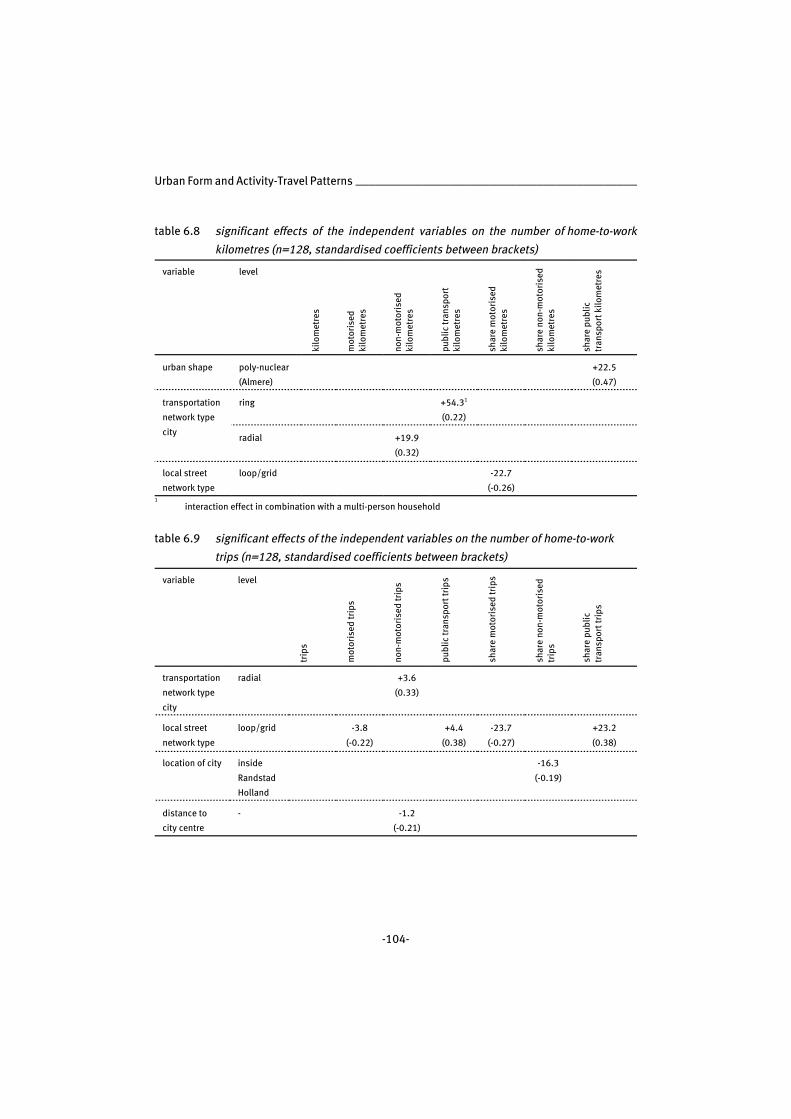
Urban Form and Activity-Travel Patterns __________________________________________
-104-
table 6.8 significant effects of the independent variables on the number of home-to-work
kilometres (n=128, standardised coefficients between brackets)
variable level
kilo
met
res
mot
oris
edki
lom
etre
s
non-
mot
oris
edki
lom
etre
s
publ
ic tr
ansp
ort
kilo
met
res
shar
e m
otor
ised
kilo
met
res
shar
e no
n-m
otor
ised
kilo
met
res
shar
e pu
blic
tran
spor
t kilo
met
res
urban shape poly-nuclear
(Almere)
+22.5
(0.47)
transportation
network type
city
ring +54.31
(0.22)
radial +19.9
(0.32)
local street
network type
loop/grid -22.7
(-0.26)1
interaction effect in combination with a multi-person household
table 6.9 significant effects of the independent variables on the number of home-to-work
trips (n=128, standardised coefficients between brackets)
variable level
trip
s
mot
oris
ed tr
ips
non-
mot
oris
ed tr
ips
publ
ic tr
ansp
ort t
rips
shar
e m
otor
ised
trip
s
shar
e no
n-m
otor
ised
trip
s
shar
e pu
blic
tran
spor
t tri
ps
transportation
network type
city
radial +3.6
(0.33)
local street
network type
loop/grid -3.8
(-0.22)
+4.4
(0.38)
-23.7
(-0.27)
+23.2
(0.38)
location of city inside
Randstad
Holland
-16.3
(-0.19)
distance to
city centre
- -1.2
(-0.21)

_______________________________________________________ Travel for Frequent Activities
-105-
trips for home-to-work trips
The numbers of trips by mode for home-to-work trips are influenced by the
transportation network types of the city and the neighbourhood, the local street network
type and the distance to the city centre (table 6.9). The number of motorised trips is
lower in loop/grid local streets, which is consistent with the effect found for motorised
kilometres. With increasing distance to the city centre the number of non-motorised
trips decreases, while it is higher in radial network cities (consistent with the effect for
kilometres). Finally, the number of public transport trips increases in loop/grid local
streets. The modal split of home-to-work trips is influenced by the local street network
type and the location of the city. The share of motorised trips is lower for loop/grid local
streets. The share of non-motorised trips is lower inside the Randstad Holland. This
could be caused by the fact the Randstad is more urbanised and has busier traffic than
non-Randstad cities, making walking and cycling less attractive options. Finally, the
share of public transport kilometres is higher with loop/grid local streets.
6.5 Summary and Conclusions
In this chapter, mode choice and the numbers of trips and kilometres for frequently
made trips were analysed. First a general description of the data was given, followed by
multilevel analysis of the data. In the general description of the data quite some
significant differences in the characteristics of the trips by urban form characteristics
were highlighted. However, the results of the multilevel analysis show few effects of
urban form characteristics on trips for grocery shopping, non-grocery shopping,
recurring leisure and home-to-work trips. Many potential relationships were analysed,
yet a limited set proved to be significant. We therefore have to conclude that, when
controlling for socioeconomic factors in a multilevel context, the effects of urban form
characteristics on trip characteristics are limited.
While controlling for socioeconomic variables describing characteristics of individuals
and households, significant effects were found for some spatial variables. It was also
found that while the effects of some urban form characteristics and their levels are
unambiguous, others show contradictory results. Table 6.10 summarises the effects for
each urban form characteristic and level for which a significant effect was found. Effects
are classified as positive, negative or undecided. An effect is considered positive when
the number of kilometres or trips is reduced, when the number of motorised kilometres

Urban Form and Activity-Travel Patterns __________________________________________
-106-
or trips is reduced and/or when the share of transport modes alternative to motorised
travel is increased. For negative effects the opposite holds. An increase in the number
of non-motorised or public transport trips or kilometres is considered undecided when
it is not accompanied by a reduction of motorised trips or kilometres.
The following characteristics can be considered positive: the poly-nuclear city (Almere),
the radial and axial transportation network neighbourhoods and the loop/grid and
loop/tree local street networks. In contrast, the ring transportation network city, the loop
and ring transportation network neighbourhoods, the loop local street network, none or
just a few shops locally available, local sports facilities available, increasing distance to
the city centre, a location inside the Randstad Holland and increasing degree of
urbanisation neighbourhood (= decreasing local address density) can be considered
negative. The results for the radial transportation network city and the small or large
neighbourhood shopping centre or city district shopping centre locally available are
undecided.
It can be concluded that these results do not strongly support hypotheses that can be
derived from literature and practice. Especially for variables describing the local
availability of services, we have not been able to unambiguously confirm the claims
described in chapter 2 and 3. For instance, none or just a few shops locally available yield
a negative effect, but better local shopping facilities do not result in a positive effect on
mobility choices. The hypotheses with regard to density, prominently present in the
international literature, can only partially be supported by our findings. In particular, it
should be noted that no effects were found for overall city density. Only neighbourhood
densities seem to be of influence, and then only for non-grocery shopping trips. The
results support the compact city concept, indicating that the use of motorised modes
increases with distance to the city centre. In contrast to literature and practice, no effects
were found for land use mix in the neighbourhood. This could be related to the fact that
medium-sized Dutch cities are so small that some degree of land use mix is always the
case, although not always within the limits of the neighbourhood as we defined them.
This chapter focussed on data on frequent activities, and therefore included a limited set
of travel motives. In the next chapter data available from the activity-travel diaries will be
analysed. These data include trips for all travel motives.

_______________________________________________________ Travel for Frequent Activities
-107-
tabl
e 6.
10su
mm
ary
of re
sult
s
urba
n fo
rm
char
acte
rist
ic
leve
ltr
avel
mot
ive
posi
tive
unde
cide
dne
gati
ve
urba
n sh
ape
poly
-
nucl
ear
(Alm
ere)
hom
e-to
-wor
k•
mor
e pu
blic
tran
spor
t
kilo
met
res
city
tran
spor
tati
on
netw
ork
type
ring
non-
groc
ery
shop
ping
•m
ore
mot
oris
ed k
ilom
etre
s (w
ith
alw
ays
car a
vaila
ble)
hom
e-to
-wor
k•
mor
e pu
blic
tran
spor
t kilo
met
res
(wit
h m
ulti
-per
son
hous
ehol
d)
radi
alho
me-
to-w
ork
•m
ore
non-
mot
oris
ed k
ilom
etre
s
•m
ore
non-
mot
oris
ed tr
ips
neig
hbou
rhoo
d
tran
spor
tati
on
netw
ork
type
loop
groc
ery
shop
ping
•la
rger
sha
re m
otor
ised
kilo
met
res
•la
rger
sha
re m
otor
ised
trip
s
non-
groc
ery
shop
ping
•sm
alle
r sha
re p
ublic
tran
spor
t
kilo
met
res
(wit
h se
cond
ary
educ
atio
n)
radi
alno
n-gr
ocer
y
shop
ping
•sm
alle
r sha
re m
otor
ised
kilo
met
res
•le
ss m
otor
ised
trip
s
axia
lno
n-gr
ocer
y
shop
ping
•sm
alle
r sha
re m
otor
ised
kilo
met
res
•le
ss m
otor
ised
trip
s
ring
non-
groc
ery
shop
ping
•la
rger
sha
re m
otor
ised
trip
s
(wit
h w
orki
ng fu
ll ti
me)

Urban Form and Activity-Travel Patterns __________________________________________
-108-
tabl
e 6.
10su
mm
ary
of re
sult
s (c
onti
nued
)
urba
n fo
rm
char
acte
rist
ic
leve
ltr
avel
mot
ive
posi
tive
unde
cide
dne
gati
ve
loca
l str
eet
netw
ork
type
loop
/gri
dno
n-gr
ocer
y
shop
ping
•le
ss n
on-m
otor
ised
trip
s (w
ith
alw
ays
car a
vaila
ble)
hom
e-to
-
wor
k
•sm
alle
r sha
re m
otor
ised
kilo
met
res
•le
ss m
otor
ised
trip
s
•m
ore
publ
ic tr
ansp
ort t
rips
•sm
alle
r sha
re m
otor
ised
trip
s
•la
rger
sha
re p
ublic
tran
spor
t
trip
s
loop
non-
groc
ery
shop
ping
•sm
alle
r sha
re n
on-m
otor
ised
kilo
met
res
loop
/tre
e
non-
groc
ery
shop
ping
•la
rger
sha
re p
ublic
tran
spor
t
trip
s
loca
l sho
ppin
g
faci
litie
s
none
or j
ust a
few
sho
ps
groc
ery
shop
ping
•le
ss o
ther
trip
s•
larg
er s
hare
mot
oris
ed
kilo
met
res
(wit
h ca
r ava
ilabl
e)
•la
rger
sha
re m
otor
ised
trip
s
(wit
h ca
r ava
ilabl
e)
smal
l
neig
hbou
rhoo
d
shop
ping
cen
tre
non-
groc
ery
shop
ping
•le
ss n
on-m
otor
ised
trip
s
larg
e
neig
hbou
rhoo
d
shop
ping
cen
tre
groc
ery
shop
ping
•sm
alle
r sha
re m
otor
ised
kilo
met
res
(wit
h w
orki
ng p
art
tim
e)
•sm
alle
r sha
re m
otor
ised
trip
s
(wit
h w
orki
ng p
art t
ime)
•m
ore
othe
r tri
ps (w
ith
wor
king
part
tim
e)
•la
rger
sha
re m
otor
ised
kilo
met
res
(wit
h w
orki
ng fu
ll
tim
e)
•m
ore
mot
oris
ed tr
ips
•le
ss o
ther
trip
s

_______________________________________________________ Travel for Frequent Activities
-109-
tabl
e 6.
10su
mm
ary
of re
sult
s (c
onti
nued
)
urba
n fo
rm
char
acte
rist
ic
leve
ltr
avel
mot
ive
posi
tive
unde
cide
dne
gati
ve
loca
l sho
ppin
g
faci
litie
s
(con
tinu
ed)
larg
e
neig
hbou
rhoo
d
shop
ping
cen
tre
(con
tinu
ed)
non-
groc
ery
shop
ping
•la
rger
sha
re p
ublic
tran
spor
t kilo
met
res
•le
ss n
on-m
otor
ised
trip
s
city
dis
tric
t
shop
ping
cen
tre
groc
ery
shop
ping
•m
ore
othe
r tri
ps
•le
ss o
ther
trip
s (w
ith
wor
king
par
t
tim
e)
loca
l spo
rts
faci
litie
s av
aila
ble
recu
rrin
g le
isur
e•
larg
er s
hare
mot
oris
ed
kilo
met
res
•m
ore
mot
oris
ed tr
ips
•le
ss o
ther
trip
s
dist
ance
to c
ity
cent
reno
n-gr
ocer
y
shop
ping
•la
rger
sha
re m
otor
ised
kilo
met
res
•la
rger
sha
re m
otor
ised
trip
s
•sm
alle
r sha
re n
on-m
otor
ised
trip
s
hom
e-to
-wor
k•
less
non
-mot
oris
ed tr
ips
loca
tion
insi
de R
ands
tad
Hol
land
groc
ery
shop
ping
•le
ss tr
ips
hom
e-to
-wor
k•
smal
ler s
hare
non
-mot
oris
ed
trip
s
degr
ee o
f urb
anis
atio
n ne
ighb
ourh
ood
(incr
ease
= d
ecre
ase
addr
ess
dens
ity)
non-
groc
ery
shop
ping
•la
rger
sha
re p
ublic
tran
spor
t kilo
met
res
•m
ore
publ
ic tr
ansp
ort k
ilom
etre
s
(eff
ect m
oder
ated
wit
h ca
r
avai
labl
e/in
crea
sed
wit
h ag
e)
•sm
alle
r sha
re n
on-m
otor
ised
trip
s (in
crea
ses
wit
h ag
e)

-110-
7 | ACTIVITY-TRAVEL PATTERNS
7.1 Introduction
As discussed in the chapter on data collection, the analyses reported in this thesis involve
two kinds of data. First, similar to most other studies into the relationship between
urban form and travel, respondents were asked to report trip frequency, distance, and
some other characteristics of frequently conducted activities. The results of these
analyses were reported in the previous chapter. However, it is well known in the
literature that these data are relatively prone to reporting bias. Moreover, a more
fundamental objection against such data is that they cannot capture all travel generated
by a household. For example, one household member reporting less car use to work may
cause other household members to use the car more, since it is available for other
purposes. Therefore, the conventional travel survey of frequently conducted activities
was supplemented with a two-day activity diary. Although such diaries are not error-free
either, they provide a more comprehensive picture of activity-travel patterns. The results
of the analyses conducted on these activity diary data are reported in this chapter.
The focus thus shifts from trips by motive to total activity-travel patterns observed for a
single day. The activity diary data described in chapter 5 were analysed in order to test
the assumed relationship between urban form characteristics and indicators of daily
travel behaviour. A multilevel analysis was conducted on a number of travel behaviour
indicators derived from the activity diaries, in order to explore more complicated
relationships between urban form and travel behaviour, while controlling for
socioeconomic characteristics of the individual and the household.
This chapter is organised as follows. Sections 7.2 and 7.3 provide a general discussion
of the diary data. In section 7.2 some characteristics of the activity-travel patterns are
presented, followed by a general description of the indicators that were derived from the
activity-travel diaries for analysis in section 7.3. Section 7.4 discusses the multilevel
____________________________________________________________ Activity-Travel Patterns
-111-
analyses applied to the data and their results. Finally, in section 7.5 conclusions will be
drawn.
7.2 Characteristics of Activity-Travel Patterns
Before addressing the analyses of the travel performance indicators derived from the
activity diaries, this section discusses the activity-travel patterns in these diaries in a
more general way. More specifically, the activity diaries were analysed using the relevant
module of the ALBATROSS model [Arentze et al, 1999; Arentze and Timmermans,
2000].
Leisure activities and work are the most common activities conducted outside the home,
closely followed by grocery shopping and bring/get activities such as bringing/getting
a child to/from school. Distinct differences can be seen in activity patterns between
mornings, afternoons and evenings (see figure 7.1). Staying at home (not making a trip)
is most common in the evening and much less in the afternoon. Home-work-home
patterns are most common in mornings and afternoons, and are rare in evenings.
Bring/get activities occur throughout the day. Service trips (post-office, hairdressers’,
etcetera) occur mainly during office hours, yet more in the afternoon than in the
morning. Trips for leisure or social activities occur more frequently later in the day. And
finally, combining several activities in one tour (trip chaining) is most common in the
afternoon. Most frequently occurring activity combinations (in one tour) are work and
service, work and social or leisure, social or leisure and service or combinations of more
activities.
Most diaries do include out-of-home activities. Only 12% of diaries do not include any
tours. A tour begins and ends at home and can include one or more stops and therefore
one or more trips. This concept is comparable to the concept of a journey in travel
research [Axhausen, 1995]. One or two tours on a day are most common. Only 15% of
all diaries include 3 or more tours. Over three quarters of all tours is a single-stop tour,
while combining more than 3 stops in a tour is very rare. Most out-of-home activities
have a considerable duration. More than half of all-out-of home activities take more than
an hour and over 30% take even more than two hours.

Urban Form and Activity-Travel Patterns __________________________________________
-112-
0
10
20
30
40
50
60
morning afternoon evening
%
no activities only in home home-work-homehome-bring/get-home home-service-home home-social/leisure-homehome-other-home more activities
figure 7.1 activity patterns by time of day
Most tours are short to very short. Almost half of all tours is (in a straight line) less than
2 kilometres long, and another quarter is between 5 and 10 kilometres (see figure 7.2).
This is also reflected in trip lengths. 38% is less than 1 kilometre long and over three
quarters is below 5 kilometres. Combining all tours for one day, we find that about one
third of the individuals do not travel more than 2 kilometres in a day, and about a
quarter travel less than 5 kilometres. The frequent occurrence of short and very short
trips is partly reflected in mode choice (see figure 7.3). Most tours are made using only
one mode of transportation and this is most often a non-motorised mode (walking or
cycling), closely followed by the car. Most common combinations of transportation
modes are motorised transport and non-motorised transport or public transport and
non-motorised transport. Other combinations are rare.
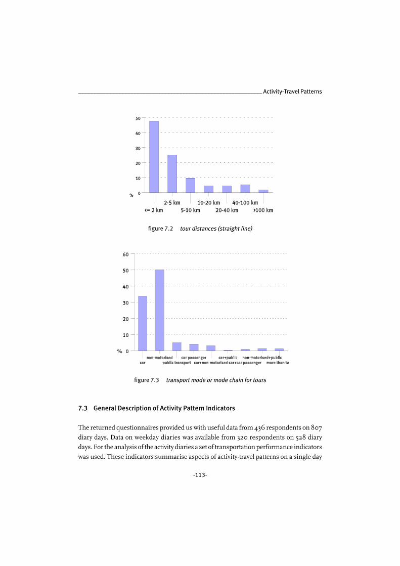
____________________________________________________________ Activity-Travel Patterns
-113-
figure 7.2 tour distances (straight line)
figure 7.3 transport mode or mode chain for tours
7.3 General Description of Activity Pattern Indicators
The returned questionnaires provided us with useful data from 436 respondents on 807
diary days. Data on weekday diaries was available from 320 respondents on 528 diary
days. For the analysis of the activity diaries a set of transportation performance indicators
was used. These indicators summarise aspects of activity-travel patterns on a single day

Urban Form and Activity-Travel Patterns __________________________________________
-114-
of a single individual and are derived from the diary data using the ALBATROSS model
[Arentze and Timmermans, 2000]. The following indicators, both for weekdays and all
days, were used in the analyses:
• total time spent travelling in minutes per day;
• total time spent travelling by motorised transport in minutes per day;
• modal split motorised transport in travel time;
• total number of trips per day;
• total number of tours per day;
• number of trips per tour, the trip/tour ratio;
• total distance travelled in kilometres per day;
• total distance travelled by motorised transport in kilometres per day;
• modal split motorised transport in travel distance.
Similar as in chapter 6, distances were measured in a straight line, based on locational
information provided by the respondents.
Below, a general description of a subset of the transportation performance indicators
will be given. Each indicator was set out against the socioeconomic and spatial variables
defined in chapter 5. For the nominal independent variables the means for each level
were calculated, while for the continuous independent variables the correlation
coefficient was obtained as a basis for the discussion. The discussion below includes only
remarks on significant differences. In order to establish whether differences between
the means and the correlations are significant, different tests were used, depending on
the nature of the variables of interest. If the assumption could be made that the variances
at the different levels of the nominal variables are equal, significance tests were based
on One-Way-ANOVA. If this assumption could not be made, the non-parametric
Kruskal-Wallis test was used. The significance of correlations was assessed using the
Pearson correlation coefficient. In appendix 6, all data is listed.
On average a diary day of the respondents included 4 trips and 1.7 tours, which means
that an average tour, starting and ending at home, included 2.4 trips. Average travel time
was 60 minutes and half of this time was spend in a motorised transport mode. Average
distance travelled on a diary day was 33 kilometres and the modal share for motorised
transport was 55%. On weekdays we find a somewhat different pattern. An average
weekday included 4.5 trips and 1.9 tours. Trip/tour ratio remains the same. Travel time
is 10 minutes longer and people travel 5 kilometres more on a weekday than on average.
Modal shares of motorised travel are comparable to the data for all diary days. Overall,

____________________________________________________________ Activity-Travel Patterns
-115-
the trip and tour frequencies and the trip/tour ratio show few differences over the
socioeconomic and spatial characteristics. Differences can mainly be found in travel time
and travel distance and more so for weekday diaries than for all diary days.
Women make more trips and tours than men, both on average and on weekdays.
However, men travel more kilometres on weekdays. The modal shares of motorised
travel time and kilometres increase with education level, both in total and for weekdays
only. Similarly, the use of motorised modes increases with personal income. Travel
distance, in total and on weekdays, is highest for those in the highest income group.
Total travel time increases with personal income. The number of tours and trips on
weekdays, is lower for lower income groups. Similar findings are obtained for work
status. Full time workers spend most time travelling, both in total and on weekdays. In
total, they also travelled the highest number of kilometres. However, on weekdays part
time workers travel more kilometres. They also have the highest number of tours, both
in total and on weekdays only. Trip-chaining is most frequent with full time workers.
People without a driver’s license make, in total, less trips and tours, their trip/tour ratio
is lower, they travel less kilometres and spend less time travelling. The picture is almost
the same for those without a car available. On weekdays, we find a similar pattern for
those without a license or car, although the differences in numbers of tours and trips
and in travel time are no longer significant. People in higher income households travel
a higher share of their weekday kilometres by motorised transport. People in two person
households make fewer trips and, on weekdays, fewer tours than people in other
household types. Trip chaining is more common for singles. The use of motorised
modes is lowest for people in families with children. People in a flat or apartment spend
most time travelling on weekdays. The share of motorised travel time on weekdays is
highest for those in a (semi)detached house.
Looking at travel behaviour by characteristics of the spatial environment, we again find
more differences on weekdays than for all diary days. Differences between transportation
network types for the city are found for weekdays only. In ring network cities travel time
and travel distance are highest, while in radial network cities they are lowest. In grid and
loop/grid type local streets people travel the highest number of kilometres, both in total
and on weekdays only. These network types also show the highest share of motorised
kilometres. In loop/tree network local streets trip frequencies are lowest. For all days, the
number of tours and the travel time are also lowest in this network type. In
neighbourhoods with ample land use mixing we find, on average, the lowest share of
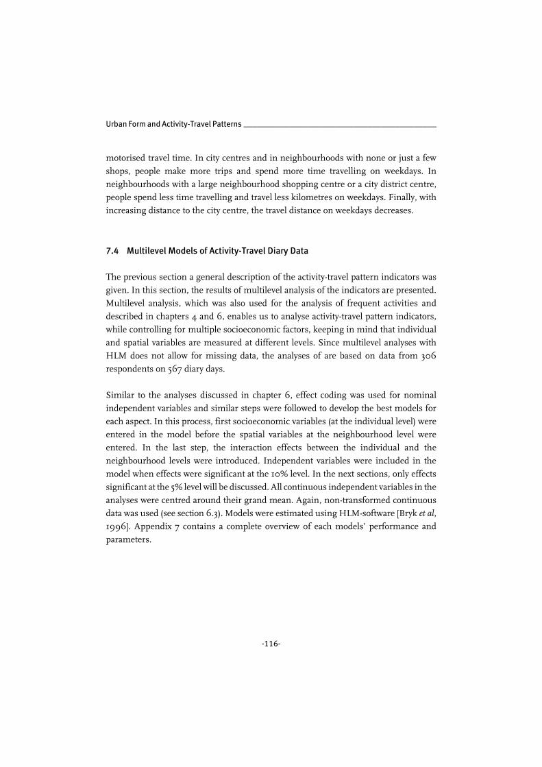
Urban Form and Activity-Travel Patterns __________________________________________
-116-
motorised travel time. In city centres and in neighbourhoods with none or just a few
shops, people make more trips and spend more time travelling on weekdays. In
neighbourhoods with a large neighbourhood shopping centre or a city district centre,
people spend less time travelling and travel less kilometres on weekdays. Finally, with
increasing distance to the city centre, the travel distance on weekdays decreases.
7.4 Multilevel Models of Activity-Travel Diary Data
The previous section a general description of the activity-travel pattern indicators was
given. In this section, the results of multilevel analysis of the indicators are presented.
Multilevel analysis, which was also used for the analysis of frequent activities and
described in chapters 4 and 6, enables us to analyse activity-travel pattern indicators,
while controlling for multiple socioeconomic factors, keeping in mind that individual
and spatial variables are measured at different levels. Since multilevel analyses with
HLM does not allow for missing data, the analyses of are based on data from 306
respondents on 567 diary days.
Similar to the analyses discussed in chapter 6, effect coding was used for nominal
independent variables and similar steps were followed to develop the best models for
each aspect. In this process, first socioeconomic variables (at the individual level) were
entered in the model before the spatial variables at the neighbourhood level were
entered. In the last step, the interaction effects between the individual and the
neighbourhood levels were introduced. Independent variables were included in the
model when effects were significant at the 10% level. In the next sections, only effects
significant at the 5% level will be discussed. All continuous independent variables in the
analyses were centred around their grand mean. Again, non-transformed continuous
data was used (see section 6.3). Models were estimated using HLM-software [Bryk et al,
1996]. Appendix 7 contains a complete overview of each models’ performance and
parameters.
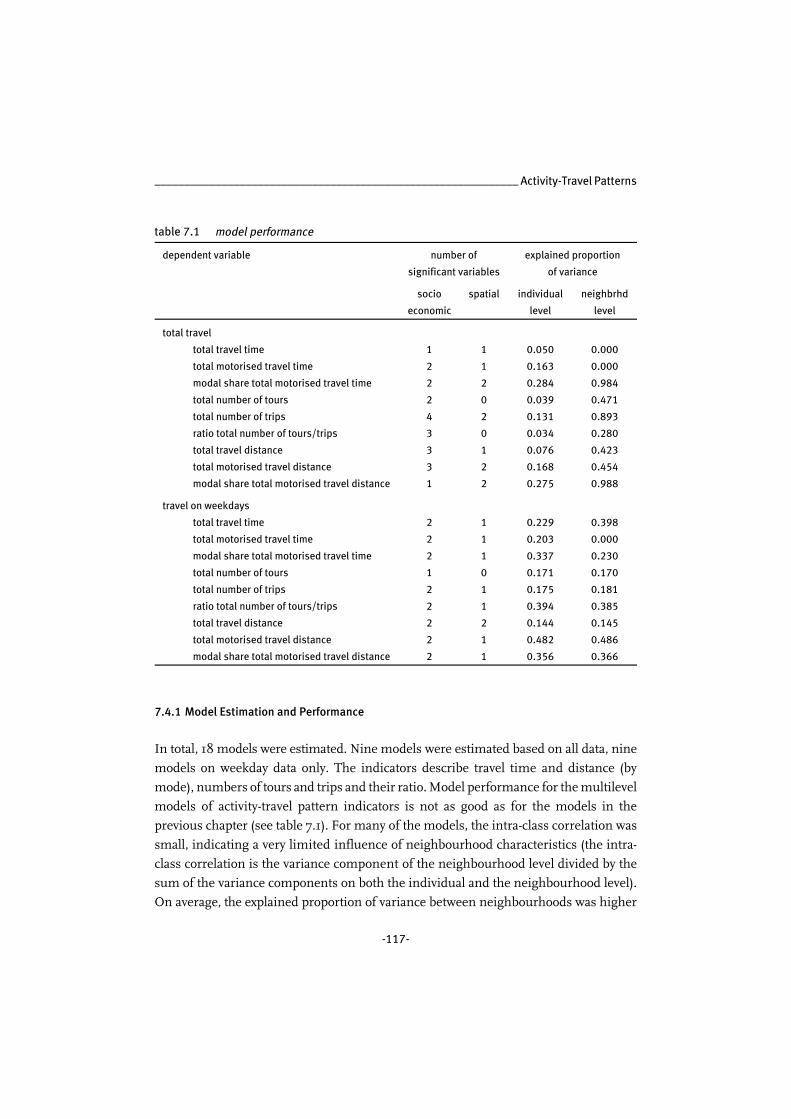
____________________________________________________________ Activity-Travel Patterns
-117-
table 7.1 model performance
dependent variable number of
significant variables
explained proportion
of variance
socio
economic
spatial individual
level
neighbrhd
level
total travel
total travel time
total motorised travel time
modal share total motorised travel time
total number of tours
total number of trips
ratio total number of tours/trips
total travel distance
total motorised travel distance
modal share total motorised travel distance
1
2
2
2
4
3
3
3
1
1
1
2
0
2
0
1
2
2
0.050
0.163
0.284
0.039
0.131
0.034
0.076
0.168
0.275
0.000
0.000
0.984
0.471
0.893
0.280
0.423
0.454
0.988
travel on weekdays
total travel time
total motorised travel time
modal share total motorised travel time
total number of tours
total number of trips
ratio total number of tours/trips
total travel distance
total motorised travel distance
modal share total motorised travel distance
2
2
2
1
2
2
2
2
2
1
1
1
0
1
1
2
1
1
0.229
0.203
0.337
0.171
0.175
0.394
0.144
0.482
0.356
0.398
0.000
0.230
0.170
0.181
0.385
0.145
0.486
0.366
7.4.1 Model Estimation and Performance
In total, 18 models were estimated. Nine models were estimated based on all data, nine
models on weekday data only. The indicators describe travel time and distance (by
mode), numbers of tours and trips and their ratio. Model performance for the multilevel
models of activity-travel pattern indicators is not as good as for the models in the
previous chapter (see table 7.1). For many of the models, the intra-class correlation was
small, indicating a very limited influence of neighbourhood characteristics (the intra-
class correlation is the variance component of the neighbourhood level divided by the
sum of the variance components on both the individual and the neighbourhood level).
On average, the explained proportion of variance between neighbourhoods was higher

Urban Form and Activity-Travel Patterns __________________________________________
-118-
than between individuals (which is consistent with the results in chapter 6) and was
higher for the total data than for the data on weekdays.
The models for the shares of total motorised travel time and distance had the highest
explained proportions of variance between neighbourhoods. From the 9 models for all
diaries, these models also had the highest explained proportion of variance between
individuals, however these figures are still below 30%. The models for total number of
trips, total number of tours, total travel distance and total motorised travel distance can
also be considered performing well. From the models for weekday diaries, only the
model for total motorised travel distance can be considered performing well, with almost
50% of variance explained both between individuals and between neighbourhoods.
7.4.2 Results of Multilevel Models
In this section the results of the multilevel analyses will be discussed. The focus will be
on the effects of the spatial independent variables. All spatial independent variables
significant at the 5% confidence level will be considered here, regardless of the values
of R2 at both levels for the models. In case of interaction effects, the accompanying
socioeconomic variable will be listed in footnotes with each table. For a complete
overview of all models, including the significant socioeconomic effects see appendix 7.
table 7.2 significant effects of the independent variables on the total number of trips and tours
and the trip/tour ratio (306 respondents, 567 diary days, standardised coefficients
between brackets)
variable level total number
of tours
total number
of trips
trip/tour ratio
transportation
network type
neighbourhood
radial -0.91 (-0.14)
axial +1.02 (0.20)
local street network
type
loop +1.13 (0.23)
grid +0.6 (0.14)1 interaction effect in combination with household income 1-2 x standard2 interaction effect in combination with working part time3 interaction effect in combination with household type couple

____________________________________________________________ Activity-Travel Patterns
-119-
total number of trips and tours
No significant effects of spatial characteristics on the total number of tours and the
trip/tour ratio were found (table 7.2). However, the number of trips is influenced by the
transportation network type of the neighbourhood and the local street network type. A
grid type local street network increases the number of trips. A similar increasing effect
was found for loop type local streets, yet only for those in a two person household. For
this household type we also found a higher number of trips when living in a
neighbourhood with an axial transportation network type. Finally, the number of trips
is lower for households with an income between 1 and 2 times standard in a
neighbourhood with a radial network.
table 7.3 significant effects of the independent variables on the number of trips and tours and
the trip/tour ratio on weekdays (225 respondents, 372 diary days, standardised
coefficients between brackets)
variable level number of
tours
number of
trips
trip/tour ratio
land use mix limited -0.6 (-0.80)
-0.51 (-0.45)
ample +0.8 (0.91)
+0.61 (-0.44)1 interaction effect in combination with higher education
trips and tours on weekdays
For the number of trips and tours and their ratio on weekdays, only the effect of land use
mix on the trip tour ratio is significant at the 5% level (table 7.3). No effects for urban
form characteristics on the number of trips and tours on weekdays were found. A
limited land use mix is related to reduced trip chaining, especially for those with higher
education. An ample land use mix yields the opposite result. The standardised
coefficients show that the first order effects are more substantial than the interaction
effects.
total travel time and distance
Again, only a few of the tested relationships proved to have significant effect (table 7.4).
The significant effects on travel time and travel distance that were found are mainly
interaction effects. In other words, these effects of spatial characteristics only hold for
certain socioeconomic groups. Travel time is hardly influenced by variables describing
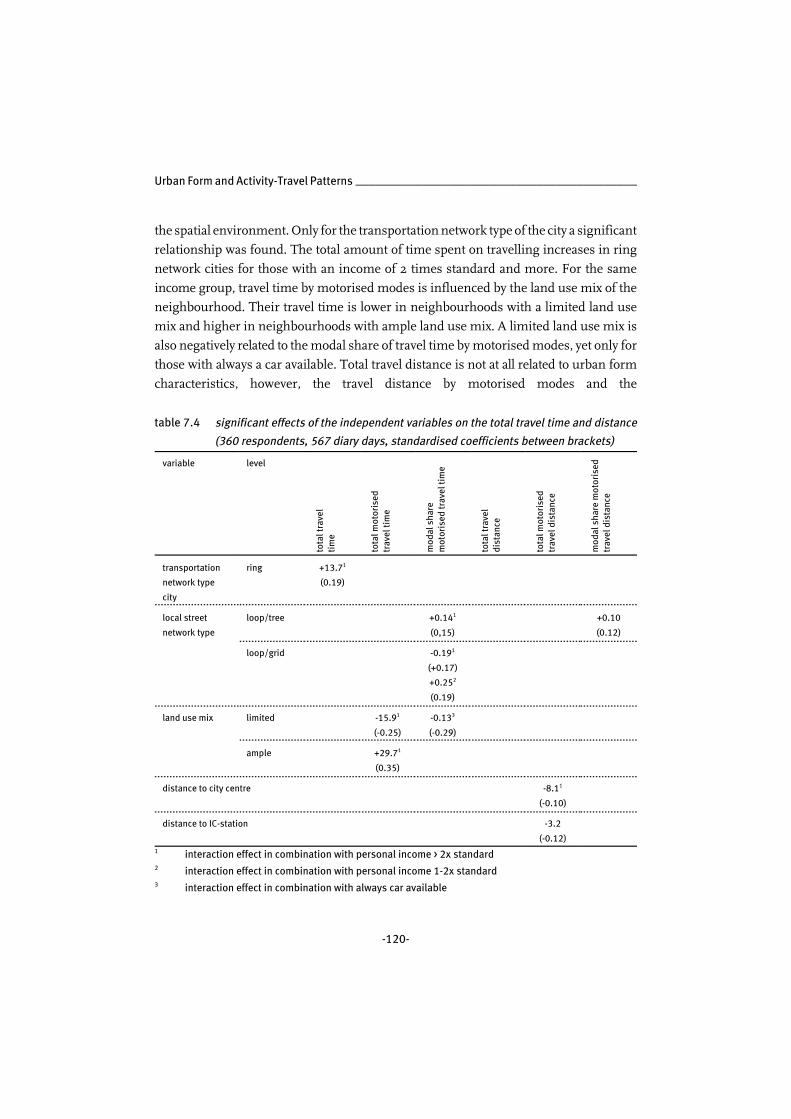
Urban Form and Activity-Travel Patterns __________________________________________
-120-
the spatial environment. Only for the transportation network type of the city a significant
relationship was found. The total amount of time spent on travelling increases in ring
network cities for those with an income of 2 times standard and more. For the same
income group, travel time by motorised modes is influenced by the land use mix of the
neighbourhood. Their travel time is lower in neighbourhoods with a limited land use
mix and higher in neighbourhoods with ample land use mix. A limited land use mix is
also negatively related to the modal share of travel time by motorised modes, yet only for
those with always a car available. Total travel distance is not at all related to urban form
characteristics, however, the travel distance by motorised modes and the
table 7.4 significant effects of the independent variables on the total travel time and distance
(360 respondents, 567 diary days, standardised coefficients between brackets)
variable level
tota
l tra
vel
tim
e
tota
l mot
oris
edtr
avel
tim
e
mod
al s
hare
mot
oris
ed tr
avel
tim
e
tota
l tra
vel
dist
ance
tota
l mot
oris
edtr
avel
dis
tanc
e
mod
al s
hare
mot
oris
edtr
avel
dis
tanc
e
transportation
network type
city
ring +13.71
(0.19)
local street
network type
loop/tree +0.141
(0,15)
+0.10
(0.12)
loop/grid -0.191
(+0.17)
+0.252
(0.19)
land use mix limited -15.91
(-0.25)
-0.133
(-0.29)
ample +29.71
(0.35)
distance to city centre -8.11
(-0.10)
distance to IC-station -3.2
(-0.12)1 interaction effect in combination with personal income > 2x standard2 interaction effect in combination with personal income 1-2x standard3 interaction effect in combination with always car available

____________________________________________________________ Activity-Travel Patterns
-121-
modal split is. The travel distance by motorised modes is lower when an inter-city station
is further away and decreases even more for those with an income of 2 times standard
or more when the distance to the city centre increases. This is a striking finding, one
would expect the opposite. Finally, the modal share of motorised transport in kilometres
is affected by the local street network type. The share for motorised transport is higher
when local streets have a loop/tree network.
travel time and distance on weekdays
When evaluating the results for travel time and distance on weekdays, we find that the
results for weekday patterns differ substantially from those pertaining to total patterns
(table 7.5). We find several effects on travel distance for weekdays, while total travel
distance was not related to urban form characteristics at all. It appears as if those who
travel many kilometres during weekdays, travel less during weekends and vice versa. On
weekdays, travel distances can be influenced (in a limited way) by the spatial
environment, yet this effect is lost when looking at all diary days. Another interesting
finding is that travel time on weekdays is not affected by urban form characteristics.
Apparently, in all types of urban forms people spend a comparable amount of time on
weekday travelling. Total travel distance proves to vary considerably with local street
network type, but only for selected groups with specific socioeconomic characteristics.
In loop, loop/tree and loop/grid network streets, couples travel less. In loop/tree network
streets, those with a minimum to standard income travel more, while they travel less in
loop/grid networks. This is also the only socioeconomic group that is sensitive to
distance to the city centre. With increasing distance to the city centre, they travel less.
This income group appears to have a small action space on weekdays, choosing
destinations near their home location. People with a slightly higher income (1-2x
standard) travel more in loop/grid networks. Travel distance on weekdays by motorised
modes is also related to local street network types. In loop/grid type streets we find
higher numbers of kilometres by motorised modes. However, the opposite is true for
couples. In grid type streets we find higher numbers of kilometres by motorised modes
for those with higher education and for couples. Finally, a small effect of population
density of the neighbourhood on the modal share of motorised travel was found. This
share increases slightly with density.

Urban Form and Activity-Travel Patterns __________________________________________
-122-
table 7.5 significant parameters travel time and distance on weekdays (225 respondents,
372 diary days, standardised coefficients between brackets)
variable level
tota
l tra
vel
tim
e
tota
l mot
oris
edtr
avel
tim
e
mod
al s
hare
mot
oris
ed tr
avel
tim
e
tota
l tra
vel
dist
ance
tota
l mot
oris
edtr
avel
dis
tanc
e
mod
al s
hare
mot
oris
edtr
avel
dis
tanc
e
local street network
type
loop -55.03
(-0.43)
loop/tree +157.94
(0.80)
-113.33
(-0.85)
loop/grid -167.64
(-0.88)
+136.92
(0.80)
-95.03
(-0.63)
+57.7
(0.59)
-67.33
(-0.54)
grid +232.03
(1.63)
+53.91
(0.44)
+72.33
(0.62)
distance to city centre - -21.54
(-0.98)
population density
neighbourhood
- +0.01
(0.30)1 interaction effect in combination with higher education2
interaction effect in combination with personal income 1-2x standard3 interaction effect in combination with household type couple4 interaction effect in combination with personal income minimum to standard
7.5 Summary and Conclusions
In this chapter, travel indicators derived from activity diaries were discussed. First a
general description of the indicators was given, Further on, they were analysed using
multilevel analysis. The indicators included the number of trips, the number of tours,
the trip/tour ratio, the total travel time, the motorised travel time, the modal share

____________________________________________________________ Activity-Travel Patterns
-123-
motorised travel time, the travel distance, the motorised travel distance and the modal
share motorised travel distance. This set of indicators was generated from the activity
diaries for weekdays only and for all days.
In chapter 6, where trips for frequent activities were analysed, few effects of urban form
characteristics on trip characteristics were found using multilevel analysis. In this
chapter, looking at total activity-travel patterns, we again find few significant results.
Where the general description of the data by spatial characteristics highlighted several
interesting differences in travel behaviour, using multilevel analysis a very limited set
of urban form characteristics was found to influence the travel indicators, most
important being the local street network type and the land use mix in the
neighbourhood. These are interesting findings. Both variables describe the spatial
characteristics of the immediate surroundings of the home and they appear to be more
important than larger scale characteristics. This is consistent with the findings of some
of the studies discussed in chapter 2, where for instance significant effects of the
presence of sidewalks were found. Furthermore, rather sizable differences in travel
distance on weekdays were found for certain socioeconomic characteristics. However,
in the analyses of all travel diaries these effects disappeared, thus indicating
compensating travel behaviour in weekends. We have to conclude that the relationship
between urban form and travel patterns is weak and that a substantial reduction of
(motorised) travel using urban form measures cannot be expected.
Table 7.6 summarises the effects for each urban form characteristic and level for which
a significant effect was found. Effects are classified as positive or negative. An effect is
considered positive when the number of kilometres or trips is reduced, when the
number of motorised kilometres or trips is reduced and/or when the share of motorised
travel is decreased. Some urban form characteristics have unambiguous positive or
negative effects. For other characteristics contradictory results were found. However,
after further deliberation, most characteristics can be classified as positive or negative,
considering for instance that an increase in travel time is less of a negative effect than
an increase in travel distance or when a negative effect is found only for a certain
socioeconomic group. Based on these considerations, the following characteristics can
be considered positive: the radial neighbourhood transportation network, limited land
use mix and increasing distance to the city centre and the inter-city train station.
Negative effects were found for the ring city transportation network, the axial
neighbourhood transportation network, the loop and loop/tree and grid local street

Urban Form and Activity-Travel Patterns __________________________________________
-124-
networks and population density of the neighbourhood. The ambiguous effects found
for loop/grid local street networks and for ample land use mix make it difficult to place
them either on the positive or on the negative side. When comparing the results to the
general description of the data, we find that some of the significant effects found with
multilevel analysis, controlling for socioeconomic factors, are consistent with the results
of the general inspection of the data. However, also contradictory results are found
These few results hardly support the hypotheses derived from the literature and practice.
Longer distances to the city centre and the inter-city train station have positive effects
(although only for specific groups), which is the opposite of the expectations. In the
analyses of frequent activities the distance to the city centre was found to have a negative
effect for non-grocery shopping, but apparently this effect does not apply to total travel
patterns. Both ample and limited land use mix show mixed results. Ample land use mix
is difficult to classify as positive or negative. However, limited land use mix tends to have
more positive than negative effects. As for the transportation network types, no clear
hypotheses were available, although the new urbanism theories propagate grid type
networks. The grid street network however scores negative in these analyses, just like
loop and loop/tree networks. A better interconnected street network makes travel easier,
therefore apparently inducing more travel.
Finally, the results of the analyses of the diaries were compared with the results of the
analyses of the frequently made trips. This comparison was possible on four dependent
variables: number of kilometres, number of motorised kilometres, modal share of
motorised kilometres and number of trips. Across all analyses we find that the number
of kilometres travelled is rather independent of the spatial environment. For none of the
frequently made trips a significant effect of spatial characteristics on the number of
kilometres was found, nor were such significant effects found for activity-travel diaries.
Weekday diaries however, do show significant effects of spatial characteristics (local
street network type and distance to the city centre) on total mobility, yet only for specific
socioeconomic groups. Significant effects on the number of motorised kilometres were
found for all diaries and for weekday diaries and for non-grocery shopping trips.
However, for each of these dependent variables, one or more different urban form
characteristics proved to have a significant effect. Again, effects were found of local street
network type and distance to the city centre, complemented with the transportation
network type of the city and the distance to the inter-city train station. The modal share
of motorised trips is significantly influenced by spatial characteristics for all frequently
____________________________________________________________ Activity-Travel Patterns
-125-
made trips and for both weekday and total diaries. Yet again, we find that for different
dependent variables, different (levels of) spatial variables show a significant effect.
Transportation network type of the neighbourhood, local street network, local facilities
(for shopping or sports) and the population density of the neighbourhood affect the
modal split. Finally, only the number of trips for grocery shopping and the number of
trips in all activity-travel diaries are affected significantly by spatial characteristics.
Different spatial characteristics for both dependent variables are found to have
significant effects. Transportation network type neighbourhood and local street network
type affect the number of trips in all diaries, while the location of the city in relation to
the Randstad affects the number of trips for grocery shopping.
This comparison of results from both motive-specific trips and activity-travel diaries
shows that for these four dependent variables, more effects are found in the analysis of
diary data than in the analysis of motive-specific trips. The effects found are rather
inconsistent. This could partly be caused by the differences in the number of cases.
However, for the few (levels of) spatial characteristics that influence more than one
dependent variable we also find that results often contradict each other. This comparison
strengthens our conclusion that the effect of urban form on travel behaviour is rather
limited. It also indicates that the analysis of complete activity-travel patterns describing
the travel behaviour of total days can lead to different conclusions on the influence of
spatial characteristics on travel behaviour.

Urban Form and Activity-Travel Patterns __________________________________________
-126-
tabl
e 7.
6su
mm
ary
of re
sult
s
urba
n fo
rmch
arac
teri
stic
leve
lpo
siti
ve e
ffec
tne
gati
ve e
ffec
t
tran
spor
tati
onne
twor
k ty
pe c
ity
ring
•m
ore
tota
l tra
vel t
ime
(wit
h in
com
e > 2
x st
anda
rd)
tran
spor
tati
onne
twor
k ty
pene
ighb
ourh
ood
radi
al•
less
trip
s (t
otal
) (w
ith
hous
ehol
d in
com
e 1-
2 x
stan
dard
)
axia
l•
mor
e tr
ips
(tot
al) (
wit
h w
orki
ng p
art t
ime)
loca
l str
eet
netw
ork
type
loop
•le
ss k
ilom
etre
s w
eekd
ays
(wit
h ho
useh
old
type
coup
le)
•m
ore
trip
s (t
otal
) (w
ith
hous
ehol
d ty
pe c
oupl
e)
loop
/tre
e•
less
kilo
met
res
on w
eekd
ays
(wit
h ho
useh
old
type
coup
le)
•hi
gher
sha
re to
tal m
otor
ised
trav
el ti
me
(wit
h in
com
e> 2
x st
anda
rd)
•m
ore
kilo
met
res
on w
eekd
ays
(wit
h in
com
e m
inim
umto
sta
ndar
d)
loop
/gri
d•
low
er s
hare
tota
l mot
oris
ed tr
avel
tim
e (w
ith
inco
me
>2x
sta
ndar
d)•
less
kilo
met
res
wee
kday
s (w
ith
inco
me
min
imum
tost
anda
rd a
nd w
ith
hous
ehol
d ty
pe c
oupl
e)•
less
mot
oris
ed k
ilom
etre
s on
wee
kday
s (w
ith
hous
ehol
d ty
pe c
oupl
e)
•hi
gher
sha
re to
tal m
otor
ised
trav
el ti
me
(wit
h in
com
e1-
2x s
tand
ard)
•m
ore
kilo
met
res
on w
eekd
ays
(wit
h in
com
e 1-
2xst
anda
rd)
•m
ore
mot
oris
ed k
ilom
etre
s on
wee
kday
s
grid
•m
ore
trip
s (t
otal
)•
mor
e ki
lom
etre
s on
wee
kday
s (w
ith
hous
ehol
d ty
peco
uple
)•
mor
e m
otor
ised
kilo
met
res
on w
eekd
ays
(wit
h hi
gher
educ
atio
n an
d w
ith
hous
ehol
d ty
pe c
oupl
e)
land
use
mix
limit
ed•
less
tota
l tra
vel t
ime
(wit
h in
com
e > 2
x st
anda
rd)
•lo
wer
sha
re to
tal m
otor
ised
trav
el ti
me
(wit
h al
way
sca
r ava
ilabl
e)•
less
trip
cha
inin
g on
wee
kday
s (e
spec
ially
wit
hhi
gher
edu
cati
on)
ampl
e•
mor
e tr
ip c
hain
ing
on w
eekd
ays
(esp
ecia
lly w
ith
high
er e
duca
tion
)•
mor
e to
tal t
rave
l tim
e (w
ith
inco
me
> 2x
stan
dard
)

____________________________________________________________ Activity-Travel Patterns
-127-
tabl
e 7.
6su
mm
ary
of re
sult
s (c
onti
nued
)
urba
n fo
rm c
hara
cter
isti
cpo
siti
ve e
ffec
tne
gati
ve e
ffec
t
dist
ance
to in
ter-
city
trai
n st
atio
n•
less
tota
l mot
oris
ed k
ilom
etre
s
dist
ance
to c
ity
cent
re•
less
tota
l mot
oris
ed k
ilom
etre
s (w
ith
inco
me
> 2x
stan
dard
)•
less
kilo
met
res
on w
eekd
ays
(wit
h in
com
e m
inim
umto
sta
ndar
d)
popu
lati
on d
ensi
ty n
eigh
bour
hood
•hi
gher
sha
re m
otor
ised
kilo
met
res
on w
eekd
ays

-128-
8 | CONCLUSIONS AND DISCUSSION
8.1 Introduction
Activity-travel patterns of individuals and households are the complex manifestation of
their pursuit of basic needs and personal preferences within the opportunities and
constraints offered by the urban environment. With this realisation in mind, this thesis
has presented the results of an extensive research project that examined the nature of
the relationship between urban form and activity-travel patterns in a Dutch context.
In the first chapters it was argued that existing spatial mobility planning practice in the
Netherlands is often based on explicit or implicit assumptions and reasoning about the
relationship between urban form and travel behaviour. Unfortunately, there is, especially
within the Netherlands, a lack of (methodologically sound) empirical evidence about the
existence of such a relationship. The studies that exist have typically focussed on single
aspects of travel behaviour as opposed to comprehensive activity-travel patterns. It is
well-known that such a focus on a single aspect, for example the work commute, may
potentially yield unrealistic and irrelevant results. When the trip to work is only short,
people may have more energy left to engage in additional evening activities and trips,
increasing their total mobility. Moreover, existing studies, both national and
international, have rarely attempted to systematically disentangle the effects of urban
form and the effects of socioeconomic factors. Socioeconomic and urban characteristics
may be strongly correlated, implying it is difficult to estimate the effects of urban
characteristics, unless appropriate methodological decisions are made.
This study was motivated by the expectation that a contribution to this field of study
could be made by conducting a methodologically more rigorous study that examines the
relationship between urban form and complete daily activity-travel patterns. The
contribution of this study to the international literature is threefold:
__________________________________________________________ Conclusions and Discussion
-129-
• It is the first study to examine the impact of urban form on comprehensive activity-
travel patterns as opposed to single motives.
• It is the first study that has used a quasi-experimental design approach to better
disentangle the effects of urban form characteristics and socioeconomic
characteristics.
• It is the first study to apply a multilevel analysis to obtain more reliable estimates of
the effects of urban form characteristics on travel behaviour.
8.2 Short Summary of the Study
The objective of this thesis was to examine the relationship between urban form
characteristics and travel patterns. An empirical study was conducted to empirically test
the implicit or explicit car mobility reduction claims, underlying Dutch mobility and land
use policies. The activity-based approach was adopted, since data on activity-travel
patterns give a more comprehensive account of travel behaviour. The approach allowed
us to examine whether the findings obtained for single activities hold if the focus shifts
to complete activity patterns.
A quasi-experimental design was chosen for data collection. Characteristics of urban
form were carefully selected for inclusion in the study, based on the literature.
Neighbourhoods for data collection were selected such that the association between
urban form characteristics and a set of socioeconomic variables is low. In 19 selected
neighbourhoods in 9 Dutch cities data on activity and travel patterns was collected by
administering activity-travel diaries. The data collected included both activity-travel diary
data and travel data on a set of frequently conducted activities. Multilevel analysis was
used for examining the data collected. Multilevel analysis is very appropriate for this
study since it allows us to identify the contribution of various variables, specified at
different levels, to the variance in the dependent variable. The independent variables in
this study were measured at the level of the individual/household and the level of the
neighbourhood. Using multilevel analysis, arbitrarily increasing the sample size for the
neighbourhood characteristics by disaggregating them to the individual level, is avoided.
The results of the analyses of both the motive-specific trip data and the complete activity-
travel diaries indicate that, when controlling for socioeconomic characteristics, the
influence of urban form on travel behaviour is limited. Only a few of the examined

Urban Form and Activity-Travel Patterns __________________________________________
-130-
relationships proved to yield significant results. Effects were found from urban shape,
transportation network types at different levels, available services and land use mix in
the neighbourhood, degree of urbanisation of the neighbourhood, population density
of the neighbourhood and distance to the city centre or inter-city train station. Note that
the effects of urban shape, available services and degree of urbanisation are only found
in the analyses of motive specific trips. More effects were found from characteristics of
the neighbourhood than from characteristics of the city. This implies that
neighbourhood design is more influential than characteristics of the city or town as a
whole. The list of independent variables that were found to be significantly related to
travel behaviour, includes variables that also frequently appears in theories, empirical
studies and policies on the relationship between urban form and travel behaviour.
However, the results from this investigation do not necessarily confirm the hypotheses
derived from the available literature. Some of the effects are the opposite of expectations
and some are only true in combination with specific socioeconomic characteristics of the
individual or household. Furthermore, only very few effects were found on total
(motorised) mobility. This leads us to the conclusion that, within the current social,
cultural and economic context, the potential of urban design as a measure to reduce
(motorised) travel in Dutch medium sized cities is very limited, yet that urban design of
neighbourhoods can influence some elements of the travel behaviour of their
inhabitants.
The evaluation of the activity-travel diary data distinguished between weekday data and
all data. It was found that differences in travel distance on weekdays can be rather sizable
for certain urban form characteristics (in combination with some socioeconomic
characteristics). In the analysis of diary data for all days, these effects disappear. This is
an indication of compensation behaviour in weekends. It appears that what is gained by
influencing weekday trips, is mostly lost in the total travel pattern. Finally, the
comparison of the results for complete activity-travel diaries and for motive-specific trips
revealed mixed results, even for the same characteristics. This indicates that the analysis
of complete activity-travel diaries can lead to different conclusions than the analysis of
motive-specific trips. Given that the analysis of travel behaviour for specific motives does
not yield results similar to the analysis of diaries, and given that activity-travel diaries
give a more comprehensive picture of travel behaviour, we argue that the analysis of
activity-travel diaries is to be preferred over the analysis of motive-specific trips when
studying the influence of the spatial environment.

__________________________________________________________ Conclusions and Discussion
-131-
8.3 Discussion of the Study
As with any study, positive and negative remarks can be made with regard to the
approach chosen and the operational decisions taken. This is intrinsic to the necessity
to make choices during the research process, and to the courses left open as a
consequence of these operational choices. In this section, some of the choices made will
be discussed. Furthermore, some critical observations will be made on the study itself.
First some remarks on choices regarding the selection independent variables. With the
recognition that travel is derived from activity participation, the researcher is snowed
under with factors that are potentially related to the matter under study, travel.
Everything influencing activity participation is also a potentially important factor for
travel analysis. In this study, we chose to focus on the effects of spatial characteristics of
the urban environment on travel, while controlling for socioeconomic characteristics of
individuals and households. This is just a subset of the extensive set of potentially
influencing factors. Cultural background or personal attitudes of households and
individuals, group attitudes and influence and other social and psychological factors have
not been taken into account. This does by no means imply that these factors can be
ignored. We are well aware of their possible effects and encourage any initiative to
examine their influence. However, they did not fit within the scope of this study.
Furthermore, based on the literature and an analysis of spatial mobility policies in the
Netherlands a set of urban form characteristics was chosen for the present study. This
is, by definition, not an exhaustive list. The study is limited to basic urban shapes,
structures and characteristics. It might be argued that urban shapes are too abstract to
identify and study. On the other hand, a typology of such urban forms belongs to the
core of urban design.
This is also the place for some critical observations regarding the methodology of the
study. The sophistication of the chosen method of analysis not only demands a high data
quality, but, in order to obtain significant relationships, also a rather large amount of
data. The analyses of data quality indicated that the data showed little bias, indicating
that our quasi-experimental design for data collection has yielded the desired result.
However, we also had to accept the fact that the response rate, and therefore the total
number of respondents, was lower than we had hoped for. The rather low total number
of cases, both in total and, consequently, by urban form characteristic, could be the cause
Urban Form and Activity-Travel Patterns __________________________________________
-132-
of a relatively low number of significant results that were found. However, this does not
influence the strength of the effects found. A larger sample size will, ceteris paribus,
only increase the significance of results, not the strength of relationships.
8.4 Recommendations for Planning and Policy
The aim of this study was to test the claims in current Dutch mobility reduction policies
that urban form characteristics can help reduce (motorised) mobility. Based on the
results of this study we have to conclude that the potential of urban design measures to
reduce the number of trips made and the number of kilometres travelled and to induce
a shift in the modal split is limited. We found a small number of effects for urban form
characteristics. However, the results found do suggest that urban form should be a factor
in policy making for mobility reduction. Characteristics such as neighbourhood network
type, street network type, land use mix, density and distance to the city centre or inter-
city station appear to be related to travel and mode choice. The radial neighbourhood
network, limited land use mix and distance to the city centre and inter-city station have
a positive effect on travel behaviour, as can be seen in the analyses of activity-travel
diaries. Negative effects are found for the ring network city, the axial network
neighbourhood, the loop, loop/tree and grid local street networks and increasing density
of the neighbourhood. Especially the results from network types give reason to pay more
attention to qualitative design characteristics, in addition to the existing attention to
quantitative measures such as density or distance. Furthermore, the finding that
neighbourhood characteristics are more influential than characteristics of the city
indicate that neighbourhood design matters.
In the introduction to this chapter, we have argued that activity-travel patterns are the
result of a complex interplay between personal needs and preferences and the
opportunities and constraints the urban environment offers. The results of this study
lead us to the conclusion that most households are not primarily driven by the
opportunities and constraints offered by the environment. Apparently, the choice of city
and the choice of neighbourhood is not heavily influenced by mobility considerations.
This finding, by the way, is consistent with the findings in housing research [Hunt et al,
1994].
__________________________________________________________ Conclusions and Discussion
-133-
Planners and policy makers should keep in mind that spatial planning and design
choices determine the characteristics of the urban environment for decades ahead. This
study has investigated the travel and activity patterns of present day people in the urban
environment of Dutch medium sized cities. In doing so, the social, cultural and
economic features of this day and age are contextual factors in the study. Results hold
for this context. In these circumstances, as argued above, it appears that the urban
environment on average poses little constraints on people’s travel and activity patterns.
Money and time appear to be sufficient to choose activity-travel patterns that fulfill the
basic needs and personal preferences best, yet might not be the most efficient from a
transportation point of view. The findings of compensation between weekdays and
weekends indicate that individuals will try to realise and optimise their desires.
Distances and/or travel time appear to play only a minor role in this context. However,
social, cultural and economic circumstances can change. The time may come that money
and time or people’s attitudes towards travel and transportation or environmental issues
change. Under such changed circumstances, the opportunities and constraints offered
by the urban environment may become more influential on people’s activity-travel
patterns. Therefore, it is important that the urban environment as it is being designed
today enables future users to employ efficient and effective travel patterns. This means
that urban design should be such that it enables people to reduce their travel by
shortening distances and it induces the choice of travel modes alternative to motorised
modes, even though the immediate effect is limited. Such a well-designed, sustainable,
urban environment may not immediately benefit (motorised) mobility reduction.
However, one should keep in mind that it may prevent substantial losses in the future.

-134-
REFERENCES
Adviesdienst Verkeer en Vervoer [1997] 7 Trends: Mobiliteit in Veranderend Nederland (7
Trends: Mobility in a Changing the Netherlands). AVV, Ministry of TPWWM,
Rotterdam.
Arentze, T., F. Hofman, N. Kalfs & H. Timmermans [1999] System for Logical
Verification and Inference of Activity (SYLVIA) Diaries. Transportation Research
Record, 1660, pp. 156-163.
Arentze, T. & H. Timmermans (eds.) [2000] ALBATROSS: A Learning Based
Transportation Oriented Simulation System. Technical University
Eindhoven/European Institute of Retailing and Services Studies, Eindhoven.
Axhausen, K. W. [1995] Travel Diary Content: a Brief Review of its Developments. Paper
presented at the 75th TRB Annual Meeting, Washington, D.C., January 1995.
Axhausen K.W. & T. Gärling [1992] Activity-Based Approaches to Travel Analysis:
Conceptual Frameworks, Models and Research Problems. Transport Reviews, 12, pp.
324-341.
Banister, D., S. Watson & C. Wood [1996] Sustainable cities: Transport, Energy and
Urban Form. Environment and Planning B: Planning and Design. 24, pp. 125-143.
Boarnet, M.G. & S. Sarmiento [1998] Can Land-use Policy Really Affect Travel
Behaviour? A Study of the Link between Non-work Travel and Land-use
Characteristics. Urban Studies, 35, pp. 1155-1169.
Bolt, D. [1982] Urban Form and Energy for Transportation, Research Centre for Physical
Planning/Organization for Applied Scientific Research: Delft.
Bryk, A.S. & S.W. Raudenbush [1992] Hierarchical Linear Models: Application and Data
Analysis Methods. Sage Publications, Newbury Park.
Bryk, A., S. Raudenbush & R. Congdon [1996] HLM Hierarchical Linear and Nonlinear
Modelling with the HLM/2L and HLM/3L Programs. Scientific Software International,
Chicago.
Bullen, N., K. Jones & C. Duncan [1997] Modelling Complexity: Analysing Between-
Individual and Between-Place Variation - a Multilevel Tutorial. Environment and
Planning A, 29, pp. 585-609.

_______________________________________________________________ References
-135-
Centraal Bureau voor de Statistiek (Statistics Netherlands) [1997] Mobiliteit in Nederland
(Mobility in the Netherlands). CBS, Voorburg/Heerlen, 1997.
Centraal Bureau voor de Statistiek (Statistics Netherlands) [1999] De Mobiliteit van de
Nederlandse Bevolking (The Mobility of the Dutch Population). CBS,
Voorburg/Heerlen.
Centraal Bureau voor de Statistiek (Statistics Netherlands) [2000] Statline.
http://statline.cbs.nl
Cervero, R. [1988] Land Use Mixing and Suburban Mobility. Transportation Quarterly,
42, pp. 429-446.
Cervero, R. [1996] Mixed Land-uses and Commuting: Evidence From the American
Housing Survey. Transport Research A, 30, pp. 361-377.
Cervero, R. & R. Gorham [1995] Commuting In Transit Versus Automobile
Neighborhoods. Journal of the American Planning Association, 61, pp. 210-225.
Cervero, R. & K. Kockelman [1997] Travel Demand and the 3 D’s: Density, Diversity and
Design. Transportation Research D, 2, pp. 199-219.
Chapin, F.S. jr. [1994] Human Activity Patterns in the City: Things People Do in Time and
Space. John Wiley & Sons, New York.
Clarke, M., M. Dix & P. Jones [1981] Error and Uncertainty in Travel Surveys.
Transportation, 10, pp. 105-126.
Congress for the New Urbanism [2000a] Website Page New Urbanism Basics.
http://www.cnu.org/newurbanism.html, page dated July 5th 2000, page accessed
August 23rd 2000.
Congress for the New Urbanism [2000b] Website Page Charter of the New Urbanism.
http://www.cnu.org/charter.html, page dated July 5th 2000, page accessed August
23rd 2000.
Coombes, M. & S. Raybould [1997] Modelling the Influence of Individual and Spatial
Factors Underlying Variations in the Levels of Secondary School Examination
Results. Environment and Planning A, 29, pp. 641-658.
Crane, R. [1996a] Cars and Drivers in the New Suburbs: Linking Access to Travel in
Neotraditional Planning. Journal of the American Planning Association, 62, pp. 51-65
Crane, R. [1996b] On Form Versus Function: Will the New Urbanism Reduce Traffic
Or Increase It? Journal of Planning Education and Research, 15, pp. 117-126.
Dijst, M. [1993] Gewijzigde Opzet van Dagboekonderzoek Succesvol (Change in layout
Diary Research Succesful). OSPA, TU Delft, Delft.

Urban Form and Activity-Travel Patterns __________________________________________
-136-
Dumbaugh, E., R. Ewing & M. Brown [2001] A Study of Internal Capture Rates for
Mixed-Use Developments in South Florida. Paper presented at the 80th TRB Annual
Meeting, Washington, D.C., January 2001.
Ettema, D.F. & H.J.P. Timmermans [1996] Activity-Based Approaches to Travel Analysis.
Pergamon, Oxford.
Ewing, R., P. Haliyur & G.W. Page [1994] Getting Around a Traditional City, a Suburban
Planned Unit Development and Everything in Between. Transportation Research
Record, 1466, pp.53-62.
Florez, J. [1998] Urban Development Patterns and Their Relationships With Travel
Behavior. Proceedings of the 26th European Transport Conference, Seminar B:
Policy, Planning and Sustainability (volume 1), Loughborough, United Kingdom,
September 1998, pp. 315-330.
Frank, L.D. & G. Pivo [1994] Impacts of Mixed Use and Density on Utilization of Three
Modes of Travel: Single Occupant Vehicle, Transit and Walking. Transportation
Research Record, 1466, pp. 37-43.
Friedman, B., S.P. Gordon & J.B. Peers [1994] Effect of Neotraditional Neighborhood
Design on Travel Characteristics. Transportation Research Record, 1466, pp. 63-70.
Gibson, G.L. [1997] New Urbanism: The Movement System and Mixed-Use Town.
Proceedings of the 25th European Transport Forum Annual Meeting, Seminar C:
Policy, Planning and Sustainability, London, 1-5 September, pp. 111-129.
Giuliano, G. & K.A. Small [1993] Is the Journey to Work Explained by Urban Structure?
Urban Studies, 30, pp. 1485-1500.
Golob, T.F. & H. Meurs [1986] Biases in Response Over Time in a Seven-Day Travel
Diary. Transportation, 10, pp. 163-181.
Gordon, I. [1997] Densities, Urban Form and Travel Behavior. Town and Country
Planning, 66, pp. 239-241.
Hägerstrand, T. [1970] What About People in Regional Science? Papers Regional Science
Association, 24, pp. 7-21.
Handy, S. [1993] Regional Versus Local Accessibility: Neo-Traditional Development and
Its Implications for Non-Work Travel. Built Environment, 18, pp. 253-267.
Handy, S. [1996] Understanding the Link Between Urban Form and Nonwork Travel.
Journal of planning Education and Research, 15, pp. 183-198.
Hanson, S. [1982] The Determinants of Daily Travel-Activity Patterns: Relative Location
and Sociodemographic Factors. Urban Geography, 3, pp. 179-202.
Housing, Spatial Planning and the Environment Council [1999] Mobiliteit met Beleid
(Handling Mobility Skilfully). HSPE Council, Den Haag.
_______________________________________________________________ References
-137-
Hox, J.J. [1995] Applied Multilevel Analysis. Amsterdam, TT Publications.
Hunt, J.D., J.D.P. McMillan & J.E. Abraham [1994] Stated Preference Investigation of
Influences on Attractiveness of Residential Locations. Transportation Research
Record, 1466, pp. 17-35.
Janse, P. [1997] Energiebesparing in Verkeer en Vervoer door Ruimtelijke Ordening (Energy
Conservation in Transportation by Spatial Planning). NOVEM, Utrecht.
Kitamura, R., P. Mokhtarian & L. Laidet [1997] A Microanalysis of Land Use and Travel
in Five Neighborhoods in the San Francisco Bay Area. Transportation, 24, pp. 125-
158.
Klerk, L.A. de [1980] Op Zoek Naar de Ideale Stad (In Search of the Ideal City). Van
Loghum Slaterus, Deventer.
Konings, J.W., H.M. Kruythoff & C. Maat [1996] Woningdichtheid en Mobiliteit. Woon-
Werkverkeer op Nieuwbouwlocaties in de Provincie Noord Brabant (Housing Density and
Mobility. Home-to-work travel in New Developments in the Province of Noord Brabant).
Delftse Universitaire Pers, Delft.
McCormack, E., P.E. Scott Rutherford & M.G. Wilkinson [2001] The Travel Impacts of
Mixed Land Use Neighbourhoods in Seattle. Paper presented at the 80th TRB
Annual Meeting, Washington, D.C., January 2001.
McNally, M.G. & S. Ryan [1993] Comparative Assessment of Travel Characteristics for
Neotraditional Designs. Transportation Research Record, 1400, pp. 67-77.
Meyburg, A.H., & W. Brög [1981] Validity Problems in Empirical Analyses of Non-
Home-Activity Patterns. Transportation Research Record, 807, pp. 46-50.
Miller, E. & A. Ibrahim [1998] Urban Form and Vehicular Travel: Some Empirical
Findings. Paper presented at the 7th annual meeting of the Transportation Research
Board, January 1998.
Ministry of Housing and Spatial Planning [1973] Derde Nota over de Ruimtelijke Ordening,
Deel 1: Oriënteringsnota (Third Report on Spatial Planning, Part 1: Orientation Report).
Staatsuitgeverij, Den Haag.
Ministry of Housing, Spatial Planning and the Environment [1985] Structuurschets voor
de Stedelijke Gebieden, deel e: Na Parlementaire Behandeling Vastgestelde Tekst(Structure Sketch for Urban Areas, Part e: Text Stipulated After Parlementary
Discussion). Ministry of HSPE, Den Haag.
Ministry of Housing, Spatial Planning and the Environment [1988] Vierde Nota over de
Ruimtelijke Ordening: Op Weg Naar 2015, deel d: Regeringsbeslissing (Fourth Report on
Spatial Planning: Set Out For 2015, Part d: Government Decision). SDU, Den Haag.
Urban Form and Activity-Travel Patterns __________________________________________
-138-
Ministry of Housing, Spatial Planning and the Environment [1990] Vierde Nota over de
Ruimtelijke Ordening Extra: Op Weg Naar 2015, deel 1: Ontwerp-PlanologischeKernbeslissing (Fourth Report on Spatial Planning Extra: Set Out For 2015, Part 1:
Concept Key Planning Decision). Den Haag.
Ministry of Housing, Spatial Planning and the Environment [1999] De Ruimte van
Nederland, Startnota Ruimtelijke Ordening 1999 (The Space of the Netherlands, Start
Memorandum Spatial Planning 1999). SDU uitgevers, Den Haag.
Ministry of Housing, Spatial Planning and the Environment [2001], Ruimte Maken,
Ruimte Delen: Vijfde Nota over de Ruimtelijke Ordening 2000-2020 (Making Space,
Sharing Space: Fifth Report on Spatial Planning 2000-2020). Staatsuitgeverij, Den
Haag.
Ministry of Housing, Spatial Planning and the Environment, Ministry of Transport,
Public Works & Water Management and Ministry of Economic Affairs [1990]Geleiding van de Mobiliteit Door een Locatiebeleid Voor Bedrijven en Voorzieningen:Werkdocument (Guiding Mobility by a Location Policy for Businesses and Institutions:
Working Document). National Spatial Planning Agency, Den Haag.
Ministry of Transport, Public Works & Water Management [1979] Structuurschema
Verkeer en Vervoer, deel d: Regeringsbeslissing (Transport Structure Scheme, Part d:
Government Decision). Staatsuitgeverij, Den Haag.
Ministry of Transport, Public Works & Water Management [1990] Tweede
Structuurschema Verkeer en Vervoer, deel d: Regeringsbeslissing (Second Transport
Structure Scheme, Part d: Government Decision). Staatsuitgeverij, Den Haag.
Ministry of Transport, Public Works & Water Management [1995] Visie op Verstedelijking
en Mobiliteit (Vision on Urbanisation and Mobility). Den Haag.
Ministry of Transport, Public Works & Water Management [1999] Perpectievennota
Verkeer en Vervoer (Transport Perspectives Memorandum). Den Haag.
Ministry of Transport, Public Works & Water Management [2000] Nationaal Verkeer en
Vervoerplan (National Traffic and Transportation Plan). Staatsuitgeverij, Den Haag.
Ministry of Transport, Public Works & Water Management and Heidemij Advies BV
[1993] Een Middelgrote Stad voor Vriendelijke Verkeer (A Medium-Sized City for
Friendly Traffic). Den Haag.
Mogridge, M.J.H. [1985] Transport, Land Use and Energy Interaction. Urban Studies, 22,
pp. 481-492.
MuConsult [2000] Mobiliteit Begint Bij de Woning. Het Effect van de Woonomgeving op de
Mobiliteit en Vervoerwijzekeuze (Mobility Starts at Home. The Effect of the Housing
Environment on Mobility and Mode Choice). Eindrapport. MuConsult, Amersfoort.

_______________________________________________________________ References
-139-
Murakami, E. & W.T. Watterson [1992] The Puget Sound Transportation Panel After
Two Waves. Transportation, 19, pp. 141-158.
Nasar, Jack. L. [1997] Neo-Traditional Development, Auto-Dependency and Sense of
Community. EDRA refereed papers, 28.
Newman, P.W.G. & J.R. Kenworthy [1989] Cities and Automobile Dependence: An
International Sourcebook. Gower Technical, Brookfield, Vt.
Niemi, I. [1993] Systematic Error in Behavioral Measurement: Comparing Results From
Interview and Time Budget Studies. Social Indicators Research, 30, pp. 229-244.
NOVEM & Ministry of Economic Affairs [19999] De Kortste Weg naar Energiebesparing
in Verkeer en Vervoer (The Shortest Path to Energy Conservation in Transportation).
Utrecht.
Næss, P. [1993] Transportation Energy in Swedish Towns and Regions. Scandinavian
Housing & Planning Research, 10, pp. 187-206.
Næss, P. [1995] Urban Form and Energy Use for Transport. A Nordic Experience. Ph.D.
Thesis. Trondheim, NTH.
Næss, P., P.G. Røe & S. Larsen [1995] Travelling Distances, Modal Split and
Transportation Energy in Thirty Residential Areas in Oslo. Journal of Environmental
Planning and Management, 38, pp. 349-370.
Næss, P. & S.L. Sandberg [1996] Workplace Location, Modal Split and Energy Use for
Commuting Trips. Urban Studies, 33, pp. 557-580.
Næss, P., S.L. Sandberg & P.G. Røe [1996] Energy Use for Transportation in 22 Nordic
Towns. Scandinavian Housing & Planning Research, 13, pp. 79-97.
Rottier, H. [1980] Stedelijke Structuren, een Inleiding Tot de Ontwikkeling van de Europese
Stad (Urban Structures, an Introduction Into the Development of the European City).
Coutinho, Muiderberg.
Røe, Per Gunnar [1999] Intra-Urban Travel and Spatial-structural Constraints: an
Investigation of Travel and Activity Patterns in 30 Residential Areas in Oslo. Paper
presented at the XIII AESOP Congress, July 7-11 1999, Bergen, Norway.
Schimek, Paul [1996] Land Use, Transit and Mode Split in Boston and Toronto. Paper
presented at the ACSP/AESOP joint international congress, July 1996, Toronto,
Canada.
Scott Rutherford, G., E. McCormack & M. Wilkinson [1996] Travel Impacts of Urban
Form: Implications From an Analysis of Two Seattle Area Travel Diaries. Paper
presented at the conference on Urban Design, Telecommuting and Travel Behavior,
Willamsburg, Virginia, October 1996.

Urban Form and Activity-Travel Patterns __________________________________________
-140-
Snellen, D., T. Arentze, A. Borgers & H. Timmermans [2001] Spatial Variability in
Response Rates and Data Quality of a Designated Day - Leave Behind - Full Activity
Diary. Paper presented at the 80th TRB Annual Meeting, Washington, D.C., January
2001.
Snijders, T.A.B. & R.J. Bosker [1999] Multilevel Analysis : an Introduction to Basic and
Advanced Multilevel Modeling. Sage, London.
Stopher, P.R. [1992] Use of an Activity-Based Diary to Collect Household Travel Data.
Transportation, 19, pp. 159-176.
Sun, Xiaoduan, Chester G. Wilmot & Tejonath Kasturi [1998] Household Travel,
Household Characteristics and Land Use: an Empirical Study From the 1994
Portland Travel Survey. Paper presented at the 1998 Annual Meeting of the
Transportation Research Board, Washington, DC.
Timmermans, H. [2000] Theories and Models of Activity Patterns. In: T. Arentze & H.
Timmermans (eds.) ALBATROSS: A Learning Based Transportation Oriented
Simulation System. Technical University Eindhoven/European Institute of Retailing
and Services Studies, Eindhoven, pp. 6-70.
Verroen, E. [1995] De Zoektocht naar Mobiliteitsbeperkende Verstedelijkingsvormen
(The Search for Mobility Reducing Urbanisation Priniciples). Rooilijn, 1995, pp. 361-
366.
Verroen, E.J., H.D. Hilbers & C.A. Smits [1995] Modeltoets Randstadvisie: de Resultaten
(Model Check Randstad Vision: the Results). Delft: TNO beleidsstudies en advies,
sector verkeer en vervoer (INRO-WG 1995-04).
World Commission on Environment and Development (WCED) [1987] Our Common
Future. Oxford University Press, Oxford.

-141-
APPENDIX 1 | Summary of Empirical Studies
This appendix includes a summary of the empirical studies discussed in chapter 3. First
the studies with the region as the unit of analysis are summarised in alphabetical order
of author, then the studies with the city as the unit of analysis are summarised in a
similar way and, finally, the studies with the neighbourhood as the unit of analysis follow
accordingly.

Urban Form and Activity-Travel Patterns __________________________________________
-142-
empi
rica
l stu
dies
at t
he re
gion
al le
vel
sour
cem
etho
dda
taco
ntro
l soc
io-
econ
omic
vari
able
s
mai
n fi
ndin
gs
Gor
don
[199
7]re
gres
sion
New
man
&Ke
nwor
thy
data
set
,
Nat
iona
l Tra
vel S
urve
y an
d
trav
el to
wor
k da
ta fr
om 1
93
regi
ons
yes
dens
ity,
siz
e, m
ix a
nd a
cces
sibi
lity
influ
ence
mod
e ch
oice
and
ene
rgy
use
Han
dy [1
993]
corr
elat
ions
aggr
egat
e da
ta o
n no
n-w
ork
trav
el fr
om th
e S
an F
ranc
isco
Bay
Are
a in
550
zon
es
nom
ixed
land
use
influ
ence
s m
ode
choi
ce fo
r
shop
ping
, but
not
the
tota
l mob
ility
Mill
er &
Ibra
him
[199
8]
regr
essi
on
(R2 =
0.4
5)
aggr
egat
e da
ta fr
om th
e To
ront
o
regi
on in
140
4 zo
nes
noce
ntra
lisat
ion
in c
ity
cent
re a
nd s
ubce
ntre
s
redu
ces
aver
age
com
mut
ing
dist
ance
Mog
ridg
e [1
995]
com
para
tive
aggr
egat
e da
ta fr
om L
ondo
n an
d
Pari
s re
gion
s
yes
limit
ed e
ffec
ts fo
und
from
den
sity
and
pub
lic
tran
spor
t pro
visi
on
Næ
ss [1
993]
regr
essi
onag
greg
ate
data
from
15
Sw
edis
h
Urb
an R
egio
ns
yes
dens
ity,
con
cent
rati
on a
nd d
egre
e of
urba
nisa
tion
exp
lain
39%
of v
aria
tion
in
ener
gy u
se
Næ
ss &
San
dber
g [1
996]
regr
essi
on
(R2 b
etw
een
0.50
and
0.16
)
disa
ggre
gate
com
mut
ing
data
from
6 c
ompa
nies
in th
e O
slo
regi
on
yes
geog
raph
ical
loca
tion
com
pany
influ
ence
s
mod
e ch
oice
and
ene
rgy
use
New
man
&
Kenw
orth
y
[198
9]
regr
essi
onag
greg
ate
data
on
wor
ldw
ide
met
ropo
litan
are
as, g
asol
ine
use
and
dens
ity
noen
ergy
con
sum
ptio
n de
crea
ses
wit
h de
nsit
y
Sch
imek
[199
6]co
mpa
rati
veag
greg
ate
data
from
Tor
onto
and
Bos
ton
regi
ons
nohi
gher
den
siti
es, g
reat
er c
once
ntra
tion
of
jobs
and
bet
ter p
ublic
tran
spor
t fac
iliti
es
indu
ce m
ore
tran
sit u
se a
nd lo
wer
car
use

______________________________________________________________________ Appendix 1
-143-
Empirical studies at the city level
empi
rica
l stu
dies
at t
he c
ity
leve
l
sour
cem
etho
dda
taco
ntro
l soc
io-
econ
omic
vari
able
s
mai
n fi
ndin
gs
Ban
iste
r, W
atso
n
& W
ood
[199
6]
step
wis
e
regr
essi
on
disa
ggre
gate
dat
a fr
om 4
Bri
tish
and
1 D
utch
cit
y, e
ach
city
stud
ied
sepa
rate
ly
yes
mix
ed la
nd u
se w
orks
whe
n bo
th q
ualit
ativ
e
and
quan
tita
tive
; den
sity
, ope
n sp
ace
and
city
size
als
o in
fluen
ce e
nerg
y us
e
Fran
k &
Piv
o
[199
4]
regr
essi
on
(R2 b
etw
een
0.14
and
0.34
)
disa
ggre
gate
dat
a on
hom
e-to
-
wor
k an
d sh
oppi
ng tr
ips
from
the
Puge
t Sou
nd s
urve
y
yes
mix
ing
of la
nd u
se a
nd p
opul
atio
n an
d jo
b
dens
ity
influ
ence
mod
e ch
oice
Næ
ss [1
993]
regr
essi
onag
greg
ate
data
from
97
Sw
edis
h
tow
ns
yes
19%
of v
aria
tion
in e
nerg
y us
e is
exp
lain
ed
by p
opul
atio
n de
nsit
y
Næ
ss, S
andb
erg
& R
øe [1
996]
regr
essi
on
(R2 =
0.7
4)
aggr
egat
e da
ta fr
om 2
2 N
ordi
c
tow
ns
yes
popu
lati
on d
ensi
ty a
nd c
once
ntra
tion
redu
ce
ener
gy u
se

Urban Form and Activity-Travel Patterns __________________________________________
-144-
empi
rica
l stu
dies
at t
he n
eigh
bour
hood
leve
l
sour
cem
etho
dda
taco
ntro
l soc
io-
econ
omic
vari
able
s
mai
n fi
ndin
gs
Cerv
ero
[198
8]st
epw
ise
regr
essi
on
(R2 b
etw
een
0.37
and
0.66
)
disa
ggre
gate
dat
a on
hom
e to
wor
k tr
ips
from
57
larg
e
subu
rban
cen
tres
in th
e U
SA
yes
sing
le o
ffic
e se
ttin
gs in
duce
sol
o co
mm
utin
g,
mix
ing
incr
ease
s al
tern
ativ
e m
odes
,
espe
cial
ly w
hen
reta
il is
ava
ilabl
e
Cerv
ero
[199
6]co
mpa
rati
ve &
regr
essi
on
(R2 =
0.4
6)
aggr
egat
e da
ta o
n m
atch
ed p
air
neig
hbou
rhoo
ds in
the
San
Fran
cisc
o B
ay A
rea
(tra
nsit
vs.
car-
orie
nted
nei
ghbo
urho
ods)
sole
ly b
y
mat
chin
g on
inco
me
resi
dent
ial d
ensi
ty a
nd tr
ansi
t fac
iliti
es
incr
ease
tran
sit u
se h
ome-
to-w
ork,
in tr
ansi
t
neig
hbou
rhoo
ds m
ore
wal
k, c
ycle
and
tran
sit
Cerv
ero
&
Gor
ham
[199
5]
regr
essi
on
(R2 =
0.5
5)
disa
ggre
gate
com
mut
ing
data
from
the
San
Fra
ncis
co B
ay A
rea
and
Sou
ther
n LA
(tra
nsit
vs.
car
-
orie
nted
nei
ghbo
urho
ods)
sole
ly b
y
mat
chin
g on
inco
me
dens
ity
and
neig
hbou
rhoo
d ty
pe a
nd th
eir
inte
ract
ion
influ
ence
tran
sit u
se to
wor
k
Cerv
ero
&
Kock
elm
an
[199
7]
regr
essi
on
(R2 b
etw
een
0.17
and
0.20
)
disa
ggre
gate
dat
a fr
om 5
0
sam
pled
nei
ghbo
urho
ods
in th
e
US
A
yes
incr
ease
d ac
cess
ibili
ty re
duce
s to
tal t
rave
l,
inte
nsit
y (c
ompo
site
var
iabl
e of
den
sity
and
land
use
mix
), v
erti
cal l
and
use
mix
and
gri
d
stre
ets
redu
ce n
on-w
ork
trav
el, h
igh
prop
orti
on o
f rec
tang
ular
blo
ck in
crea
se to
tal
and
non-
wor
k tr
avel
Dum
baug
h, E
win
g
& B
row
n [2
001]
regr
essi
on
(R2 =
0.4
7)
aggr
egat
e da
ta fr
om 2
2
neig
hbou
rhoo
ds in
Sou
th F
lori
da
noin
tern
al c
aptu
re ra
tes
(rat
e of
trip
s w
ithi
n
area
) are
hig
her i
n hi
gh d
ensi
ty
neig
hbou
rhoo
ds w
ith
com
mer
cial
func
tion
s
and
a jo
bs/h
ousi
ng b
alan
ce c
ompa
rabl
e to
the
tota
l reg
ion

______________________________________________________________________ Appendix 1
-145-
sour
cem
etho
dda
taco
ntro
l soc
io-
econ
omic
vari
able
s
mai
n fi
ndin
gs
Ewin
g, H
aliy
ur &
Page
[199
4]
com
para
tive
(AN
OVA
)
aggr
egat
e da
ta fr
om a
dia
ry
base
d su
rvey
in s
ix
neig
hbou
rhoo
ds in
Flo
rida
sole
ly b
y
mat
chin
g on
inco
me
high
den
sity
and
land
use
mix
redu
ce u
se o
f
mot
oris
ed tr
ansp
ort
Flor
ez [1
998]
com
para
tive
disa
ggre
gate
dat
a fr
om 3
neig
hbou
rhoo
ds in
Car
acas
(tra
diti
onal
vs.
clu
ster
ed
neig
hbou
rhoo
ds)
sole
ly b
y
mat
chin
g on
inco
me
in tr
adit
iona
l nei
ghbo
urho
ods
less
car
use
,
mor
e tr
ansi
t use
and
low
er tr
avel
tim
e
Frie
dman
, Gor
don
& P
eers
[199
4]
com
para
tive
aggr
egat
e da
ta fr
om S
an
Fran
cisc
o (t
radi
tion
al v
s.
stan
dard
sub
urba
n)
mat
chin
g on
inco
me
and
hous
ing
pric
e
stan
dard
sub
urba
n ne
ighb
ourh
oods
sho
w
high
er tr
ip ra
tes
(bot
h to
tal a
nd b
y ca
r)
Han
dy [1
996]
com
para
tive
(AN
OVA
)
disa
ggre
gate
dat
a fr
om 4
neig
hbou
rhoo
ds in
San
Fra
ncis
co
Bay
Are
a (m
oder
n vs
. tra
diti
onal
)
mat
chin
ghi
gher
acc
essi
bilit
y gi
ves
shor
ter t
rips
, hig
her
trip
freq
uenc
y an
d m
ore
wal
king
, hig
her
acce
ssib
ility
in c
ombi
nati
on w
ith
mor
e
vari
atio
n in
des
tina
tion
s gi
ves
long
er tr
ips
Han
son
[198
2]re
gres
sion
(R2 b
etw
een
0.10
and
0.43
)
disa
ggre
gate
dat
a fr
om th
e
Upp
sala
trav
el d
iary
yes
mix
ing
of fu
ncti
ons
near
hom
e or
wor
kpla
ce
influ
ence
s tr
avel
beh
avio
ur
Kita
mur
a,
Mok
htar
ian
&
Laid
et [1
997]
regr
essi
on
(R2 b
etw
een
0.03
and
0.16
)
disa
ggre
gate
dat
a fr
om tr
avel
diar
ies
in 5
San
Fra
ncis
co B
ay
Area
nei
ghbo
urho
ods
yes
resi
dent
ial d
ensi
ty, p
ublic
tran
spor
t
acce
ssib
ility
, mix
ed la
nd u
se a
nd h
avin
g si
de
wal
ks in
fluen
ce n
umbe
r of t
rips
and
mod
e
choi
ce

Urban Form and Activity-Travel Patterns __________________________________________
-146-
sour
cem
etho
dda
taco
ntro
l soc
io-
econ
omic
vari
able
s
mai
n fi
ndin
gs
Koni
ngs,
Kruy
thof
f & M
aat
[199
6]
regr
essi
on
(R2 =
0.1
8)
disa
ggre
gate
dat
a fr
om 9
09
rece
ntly
mov
ed h
ouse
hold
s in
new
ly d
evel
oped
are
as in
the
Net
herl
ands
yes
no e
ffec
t fro
m s
pati
al v
aria
bles
in re
gres
sion
anal
ysis
MuC
onsu
lt [2
000]
regr
essi
on
(R2 b
etw
een
0.08
and
0.40
)
disa
ggre
gate
dat
a fr
om 7
13
resp
onde
nts
in th
e N
ethe
rlan
ds
yes
trav
el d
ista
nce
is in
fluen
ced
by s
tree
t typ
e,
dens
ity
and
wal
k/cy
cle
frie
ndlin
ess,
num
ber
of tr
ips
is in
fluen
ced
by s
tree
t typ
e an
d
acce
ssib
ility
of s
hopp
ing
faci
litie
s
Næ
ss, R
øe &
Lars
en [1
995]
regr
essi
on
(R2 b
etw
een
0.37
and
0.58
)
disa
ggre
gate
dat
a fr
om 3
0
resi
dent
ial a
reas
in O
slo
yes
dist
ance
to d
ownt
own
influ
ence
s to
tal t
rave
l
dist
ance
and
ene
rgy
use,
resi
dent
ial d
ensi
ty
influ
ence
s pu
blic
tran
spor
t use
and
loca
l
serv
ice
acce
ssib
ility
influ
ence
s en
ergy
use
Nas
ar [1
997]
com
para
tive
disa
ggre
gate
dat
a fr
om 2
neig
hbou
rhoo
ds in
Ohi
o
(neo
trad
itio
nal v
s. s
ubur
ban)
yes
smal
l diff
eren
ces
betw
een
neig
hbou
rhoo
ds
foun
d fo
r tot
al n
umbe
r of t
rips
and
som
e tr
ip
purp
oses
Røe
[199
9]re
gres
sion
(R2 b
etw
een
0.09
and
0.26
)
disa
ggre
gate
dat
a fr
om 4
00
resp
onde
nts
in 3
0 re
side
ntia
l
neig
hbou
rhoo
ds in
Osl
o
yes
dist
ance
from
hom
e to
wor
k an
d di
stan
ce fr
om
hom
e to
pri
vate
ser
vice
s in
fluen
ce to
tal t
rave
l
dist
ance
and
tim
e, d
ista
nce
from
hom
e to
cit
y
cent
re in
fluen
ce to
tal t
rave
l dis
tanc
e
Sco
tt R
uthe
rfor
d,
McC
orm
ack
&
Wilk
inso
n [1
996]
com
para
tive
aggr
egat
e da
ta fr
om tr
avel
dia
ries
in 4
Sea
ttle
nei
ghbo
urho
ods
yes,
but
limit
ed
mix
ed la
nd u
se is
link
ed to
less
trav
el

______________________________________________________________________ Appendix 1
-147-
sour
cem
etho
dda
taco
ntro
l soc
io-
econ
omic
vari
able
s
mai
n fi
ndin
gs
Sun
, Wilm
ot &
Kast
uri [
1998
]
regr
essi
on
(R2 b
etw
een
0.37
and
0.68
)
disa
ggre
gate
dat
a fr
om th
e
Port
land
trav
el s
urve
y
yes
land
use
bal
ance
and
acc
essi
bilit
y in
fluen
ce
tota
l tra
vel,
no in
fluen
ce o
f spa
tial
var
iabl
es
on n
umbe
r of t
rips
McC
orm
ack,
Ruth
erfo
rd &
Wilk
inso
n [2
001)
ANO
VAag
greg
ate
data
from
trav
el d
iari
es
in S
eatt
le R
egio
n an
d 3
mix
ed
land
use
nei
ghbo
urho
ods
yes,
but
limit
ed
mix
ed la
nd u
se is
link
ed to
less
kilo
met
res
trav
elle
d, a
nd m
ore
use
of w
alki
ng a
nd
tran
sit;
no
effe
ct fo
und
on tr
avel
tim
e

-148-
APPENDIX 2 | City and Neighbourhood Characteristics
Almere
characteristic level
urban shape poly-nuclear
city road network type ring
location inside Randstad
employment (jobs/1000 inhabitants) 251
population density (per hectare) 9
housing density (per hectare) 4
degree of urbanisation 3
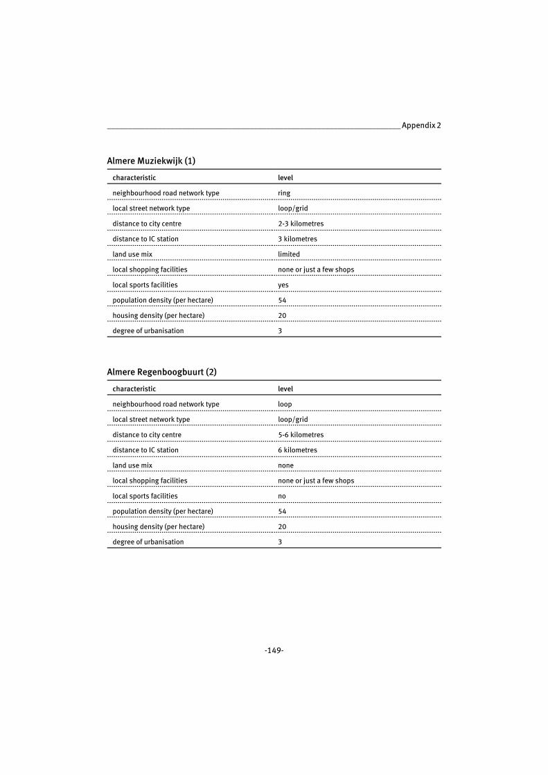
______________________________________________________________________ Appendix 2
-149-
Almere Muziekwijk (1)
characteristic level
neighbourhood road network type ring
local street network type loop/grid
distance to city centre 2-3 kilometres
distance to IC station 3 kilometres
land use mix limited
local shopping facilities none or just a few shops
local sports facilities yes
population density (per hectare) 54
housing density (per hectare) 20
degree of urbanisation 3
Almere Regenboogbuurt (2)
characteristic level
neighbourhood road network type loop
local street network type loop/grid
distance to city centre 5-6 kilometres
distance to IC station 6 kilometres
land use mix none
local shopping facilities none or just a few shops
local sports facilities no
population density (per hectare) 54
housing density (per hectare) 20
degree of urbanisation 3

Urban Form and Activity-Travel Patterns __________________________________________
-150-
Apeldoorn
characteristic level
urban shape concentric
city road network type grid
location outside Randstad
employment (jobs/1000 inhabitants) 433
population density (per hectare) 4
housing density (per hectare) 2
degree of urbanisation 3

______________________________________________________________________ Appendix 2
-151-
Apeldoorn Matenveld/donk (3)
characteristic level
neighbourhood road network type ring
local street network type loop
distance to city centre 3-4 kilometres
distance to IC station 4 kilometres
land use mix limited
local shopping facilities large neighbourhood shopping centre
local sports facilities yes
population density (per hectare) 65
housing density (per hectare) 23
degree of urbanisation 2
Apeldoorn Ugchelen (4)
characteristic level
neighbourhood road network type radial
local street network type loop/tree
distance to city centre 4-5 kilometres
distance to IC station 5 kilometres
land use mix limited
local shopping facilities small neighbourhood shopping centre
local sports facilities yes
population density (per hectare) 21
housing density (per hectare) 8
degree of urbanisation 4
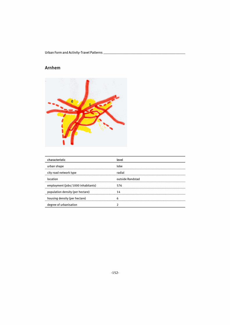
Urban Form and Activity-Travel Patterns __________________________________________
-152-
Arnhem
characteristic level
urban shape lobe
city road network type radial
location outside Randstad
employment (jobs/1000 inhabitants) 576
population density (per hectare) 14
housing density (per hectare) 6
degree of urbanisation 2

______________________________________________________________________ Appendix 2
-153-
Arnhem Alteveer/Cranevelt (5)
characteristic level
neighbourhood road network type axial
local street network type loop/tree
distance to city centre 2-3 kilometres
distance to IC station 3 kilometres
land use mix none
local shopping facilities small neighbourhood shopping centre
local sports facilities yes
population density (per hectare) 36
housing density (per hectare) 17
degree of urbanisation 4
Arnhem Presikhaaf (6)
characteristic level
neighbourhood road network type axial
local street network type loop
distance to city centre 3-4 kilometres
distance to IC station 5 kilometres
land use mix limited
local shopping facilities city district shopping centre
local sports facilities yes
population density (per hectare) 40
housing density (per hectare) 21
degree of urbanisation 2

Urban Form and Activity-Travel Patterns __________________________________________
-154-
Den Haag
characteristic level
urban shape grid
city road network type grid
location inside Randstad
employment (jobs/1000 inhabitants) 459
population density (per hectare) 65
housing density (per hectare) 31
degree of urbanisation 1

______________________________________________________________________ Appendix 2
-155-
Den Haag Centrum (7)
characteristic level
neighbourhood road network type grid
local street network type grid
distance to city centre 0-1 kilometres
distance to IC station 2 kilometres
land use mix ample
local shopping facilities city centre
local sports facilities no
population density (per hectare) 40
housing density (per hectare) 21
degree of urbanisation 1
Den Haag Berestein (8)
characteristic level
neighbourhood road network type grid
local street network type loop
distance to city centre 5-6 kilometres
distance to IC station 4 kilometres
land use mix limited
local shopping facilities large neighbourhood shopping centre
local sports facilities yes
population density (per hectare) 69
housing density (per hectare) 34
degree of urbanisation 1

Urban Form and Activity-Travel Patterns __________________________________________
-156-
Den Haag Voorburg Essesteijn (9)
characteristic level
neighbourhood road network type axial
local street network type tree
distance to city centre 3-4 kilometres
distance to IC station 6 kilometres
land use mix none
local shopping facilities small neighbourhood shopping centre
local sports facilities yes
population density (per hectare) 38
housing density (per hectare) 20
degree of urbanisation 1

______________________________________________________________________ Appendix 2
-157-
Eindhoven
characteristic level
urban shape lobe
city road network type ring/radial
location outside Randstad
employment (jobs/1000 inhabitants) 580
population density (per hectare) 23
housing density (per hectare) 10
degree of urbanisation 2

Urban Form and Activity-Travel Patterns __________________________________________
-158-
Eindhoven Stratum (10)
characteristic level
neighbourhood road network type radial
local street network type grid
distance to city centre 1-2 kilometres
distance to IC station 2 kilometres
land use mix none
local shopping facilities small neighbourhood shopping centre
local sports facilities no
population density (per hectare) 38
housing density (per hectare) 20
degree of urbanisation 1
Eindhoven Achtse Barrier (11)
characteristic level
neighbourhood road network type ring
local street network type loop
distance to city centre 5-6 kilometres
distance to IC station 6 kilometres
land use mix limited
local shopping facilities small neighbourhood shopping centre
local sports facilities yes
population density (per hectare) 61
housing density (per hectare) 22
degree of urbanisation 3

______________________________________________________________________ Appendix 2
-159-
Enschede
characteristic level
urban shape concentric
city road network type radial
location outside Randstad
employment (jobs/1000 inhabitants) 381
population density (per hectare) 11
housing density (per hectare) 4
degree of urbanisation 2

Urban Form and Activity-Travel Patterns __________________________________________
-160-
Enschede Stadsveld/Bruggert (12)
characteristic level
neighbourhood road network type radial
local street network type grid
distance to city centre 2-3 kilometres
distance to IC station 3 kilometres
land use mix none
local shopping facilities large neighbourhood shopping centre
local sports facilities yes
population density (per hectare) 58
housing density (per hectare) 26
degree of urbanisation 2
Enschede Helmerhoek Zuid (13)
characteristic level
neighbourhood road network type tangential
local street network type loop
distance to city centre 4-5 kilometres
distance to IC station 5 kilometres
land use mix none
local shopping facilities small neighbourhood shopping centre
local sports facilities yes
population density (per hectare) 89
housing density (per hectare) 31
degree of urbanisation 3

______________________________________________________________________ Appendix 2
-161-
Haarlem
characteristic level
urban shape grid
city road network type grid
location inside Randstad
employment (jobs/1000 inhabitants) 407
population density (per hectare) 50
housing density (per hectare) 22
degree of urbanisation 1
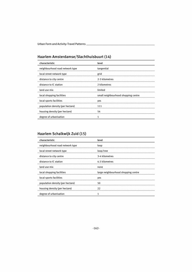
Urban Form and Activity-Travel Patterns __________________________________________
-162-
Haarlem Amsterdamse/Slachthuisbuurt (14)
characteristic level
neighbourhood road network type tangential
local street network type grid
distance to city centre 2-3 kilometres
distance to IC station 2 kilometres
land use mix limited
local shopping facilities small neighbourhood shopping centre
local sports facilities yes
population density (per hectare) 111
housing density (per hectare) 54
degree of urbanisation 1
Haarlem Schalkwijk Zuid (15)
characteristic level
neighbourhood road network type loop
local street network type loop/tree
distance to city centre 3-4 kilometres
distance to IC station 4.5 kilometres
land use mix none
local shopping facilities large neighbourhood shopping centre
local sports facilities yes
population density (per hectare) 50
housing density (per hectare) 22
degree of urbanisation 1

______________________________________________________________________ Appendix 2
-163-
Leeuwarden
characteristic level
urban shape grid
city road network type ring
location outside Randstad
employment (jobs/1000 inhabitants) 615
population density (per hectare) 11
housing density (per hectare) 26
degree of urbanisation 2
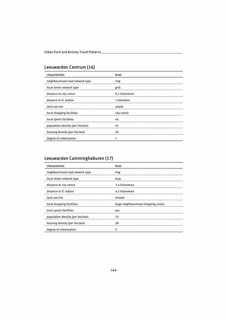
Urban Form and Activity-Travel Patterns __________________________________________
-164-
Leeuwarden Centrum (16)
characteristic level
neighbourhood road network type ring
local street network type grid
distance to city centre 0-1 kilometres
distance to IC station 1 kilometre
land use mix ample
local shopping facilities city centre
local sports facilities no
population density (per hectare) 41
housing density (per hectare) 26
degree of urbanisation 1
Leeuwarden Camminghaburen (17)
characteristic level
neighbourhood road network type ring
local street network type loop
distance to city centre 3-4 kilometres
distance to IC station 4.5 kilometres
land use mix limited
local shopping facilities large neighbourhood shopping centre
local sports facilities yes
population density (per hectare) 70
housing density (per hectare) 28
degree of urbanisation 3
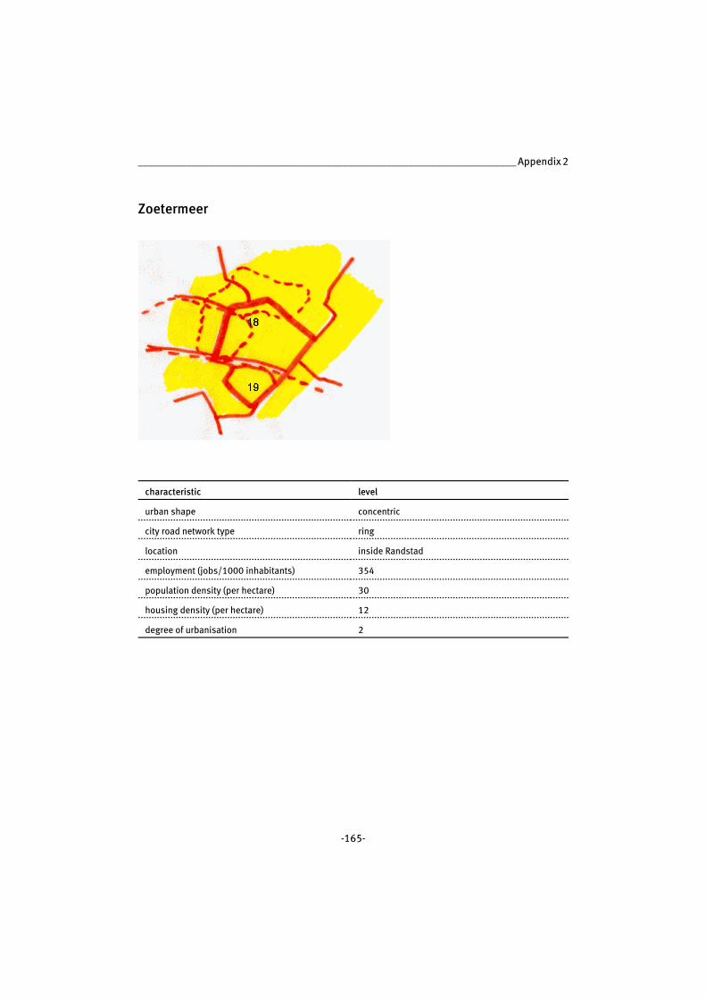
______________________________________________________________________ Appendix 2
-165-
Zoetermeer
characteristic level
urban shape concentric
city road network type ring
location inside Randstad
employment (jobs/1000 inhabitants) 354
population density (per hectare) 30
housing density (per hectare) 12
degree of urbanisation 2
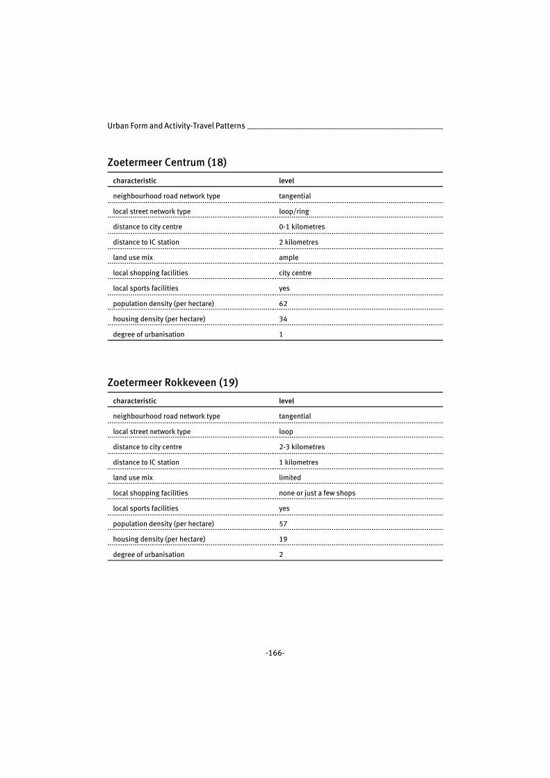
Urban Form and Activity-Travel Patterns __________________________________________
-166-
Zoetermeer Centrum (18)
characteristic level
neighbourhood road network type tangential
local street network type loop/ring
distance to city centre 0-1 kilometres
distance to IC station 2 kilometres
land use mix ample
local shopping facilities city centre
local sports facilities yes
population density (per hectare) 62
housing density (per hectare) 34
degree of urbanisation 1
Zoetermeer Rokkeveen (19)
characteristic level
neighbourhood road network type tangential
local street network type loop
distance to city centre 2-3 kilometres
distance to IC station 1 kilometres
land use mix limited
local shopping facilities none or just a few shops
local sports facilities yes
population density (per hectare) 57
housing density (per hectare) 19
degree of urbanisation 2

-167-
APPENDIX 3 | Definitions of Socioeconomic Variables
education level
The variable ‘education level’ refers to the highest education level successfully finished
by the individual in question. Three levels are discerned: no education or just primary
school, secondary education (general or vocational) and higher education (higher
vocational or university).
personal income
Personal income refers to the individual net income per year. Income has been classified
based on the standard income as used by Statistics Netherlands (website). The standard
income is the income of a standard employee. A standard employee is an employee with
two children below the age of 12 and an income just below the income limit for the
Dutch national health service (ziekenfondsgrens). The following categories are
discerned: below minimum (yearly income below approximately 15,000 guilders),
between minimum and standard (yearly income between 15,000 and 30,000 guilders
approximately), between standard and 2x standard (yearly income between 30,000 and
50,000 guilders approximately) and 2x standard and more (yearly income over 50,000
guilders).
driver’s license possession
Driver’s license possession is a personal characteristic describing whether or not the
individual has a driver’s license.
employment status
This variable indicates whether a person is not employed, part time employed or full
time employed. Employment is considered part time when a person works less than 32
hours per week. Voluntary work that has a regular recurring pattern is also treated as a
job.
Urban Form and Activity-Travel Patterns __________________________________________
-168-
car availability
Car availability is defined on the individual level in three categories: no car available,
always a car available (main user of a car in the household) and sometimes a car available
(secondary user of a car in the household or car shared with others outside the
household).
household income
Household income has been calculated from the data available on the personal incomes
of each of the household members. The variable is categorised based on the standard
income, in the same categories as are used for personal income.
household type
As household type were distinguished singles, couples and families with children.
dwelling type
‘Dwelling type’ refers to the type of house the household in question lives in. Distinction
is made between flats or apartments, terraced housing and (semi)detached housing.
average distance to chosen location (for analysis of frequent activities only)
This variable describes the average distance from home to the chosen locations for
recurring trips such as (grocery) shopping, sports and work. In this study, the distance
to the chosen location per trip or average distance to the chosen locations per individual
are considered variables at the individual level, since choice for a location is a personal
choice and can be influenced by many factors. From tentative linear regression analysis
it was found that for the travel motives grocery shopping, non-grocery shopping and
recurring leisure, this distance per trip cannot be explained by the other spatial and
socioeconomic variables included in the research. For home-to-work trips it was found
that personal income and gender are related to the distance to the chosen location. For
the average distance to chosen location per individual, a multi level analysis showed that
again for the motives grocery shopping, non-grocery shopping and recurring leisure, the
average distance cannot be explained by the other spatial and socioeconomic variables.
For home-to-work trips, gender, age, household income and employment in the city
were significantly related to average distance.

-169-
APPENDIX 4 | General Description Frequent Activities
The tables listed below contain the figures that go with the general description of the
frequent activities data reported on in section 6.2. The tables for grocery shopping and
recurring leisure activities include data on total number of kilometres travelled and trips
made, as well as the modal share for motorised kilometres and trips. The tables for non-
grocery shopping and home-to-work trips include data on total number of kilometres
travelled and trips made, as well as the modal shares for motorised, non-motorised and
public transport kilometres and trips.
Cells that contain significant differences at the 5% level are grey. For the ordinal
independent variables, significance of differences has been established using one-way
ANOVA or the Kruskal Wallis test, depending on whether the variances between groups
could be considered equal. For the continuous independent variables Pearson correlation
coefficient was calculated.

Urban Form and Activity-Travel Patterns __________________________________________
-170-
travel characteristics grocery shopping by individual and household characteristics (n=392)
kilometres modal share
motorised kilometres
trips modal share motorised
trips
total 19.5 0.39 15 0.35
gendermen
women
21.4
19.3
0.45
0.37
13.6
15.6
0.41
0.32
education level
none or primarysecondary
higher
10.218.6
23.5
0.140.42
0.40
12.415.8
13.8
0.130.37
0.35
personal income
< minimumminimum to standard
1-2x standard> 2x standard
30.212.7
9.535.0
0.230.34
0.430.44
17.216.0
12.413.8
0.250.27
0.390.52
work statusnot
part timefull time
16.9
28.417.6
0.33
0.290.49
19.2
14.911.1
0.28
0.270.46
driver’s licenseno
yes
11.5
22.1
0.13
0.46
17.1
14.3
0.12
0.41
car available
noyes
11.322.7
0.110.48
16.514.3
0.100.43
household income< standard
app. standard1-2x standard
> 2x standard
10.2
10.213.1
27.4
0.24
0.260.45
0.44
16.0
15.413.9
14.7
0.23
0.230.42
0.40
household type
singlecouple
family with children
10.123.6
20.8
0.360.42
0.39
15.615.2
14.4
0.280.37
0.37
dwelling type
flat/apartmentterraced
(semi)detached
9.918.3
33.6
0.250.43
0.45
14.215.5
14.9
0.210.38
0.45
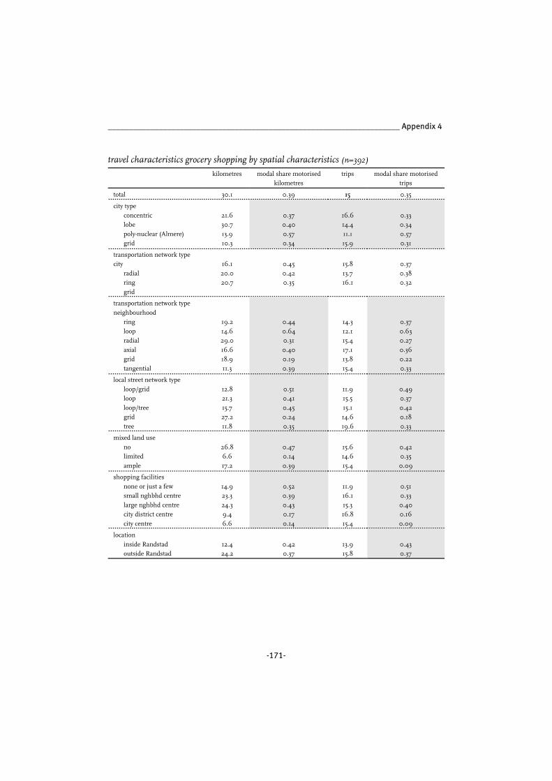
_____________________________________________________________________ Appendix 4
-171-
travel characteristics grocery shopping by spatial characteristics (n=392)
kilometres modal share motorisedkilometres
trips modal share motorisedtrips
total 30.1 0.39 15 0.35
city type
concentriclobe
poly-nuclear (Almere)grid
21.630.7
13.910.3
0.370.40
0.570.34
16.614.4
11.115.9
0.330.34
0.570.31
transportation network typecity
radialring
grid
16.1
20.020.7
0.45
0.420.35
15.8
13.716.1
0.37
0.380.32
transportation network type
neighbourhoodring
loopradial
axialgrid
tangential
19.2
14.629.0
16.618.9
11.3
0.44
0.640.31
0.400.19
0.39
14.3
12.115.4
17.113.8
15.4
0.37
0.630.27
0.360.22
0.33
local street network type
loop/gridloop
loop/treegrid
tree
12.821.3
15.727.2
11.8
0.510.41
0.450.24
0.35
11.915.5
15.114.6
19.6
0.490.37
0.420.18
0.33
mixed land use
nolimited
ample
26.86.6
17.2
0.470.14
0.39
15.614.6
15.4
0.420.35
0.09
shopping facilities
none or just a fewsmall nghbhd centre
large nghbhd centrecity district centre
city centre
14.923.3
24.39.4
6.6
0.520.39
0.430.17
0.14
11.916.1
15.316.8
15.4
0.510.33
0.400.16
0.09
location
inside Randstadoutside Randstad
12.424.2
0.420.37
13.915.8
0.430.37

Urban Form and Activity-Travel Patterns __________________________________________
-172-
correlation coefficients grocery shopping (n=392)
kilometres
(n=338)
modal share
motorised
kilometres
(n=325)
trips (n=392) modal share
motorised
trips (n=392)
age -0.06 0 0.26 0
distance to city centre -0.06 0.13 0.04 0.16
distance to ic station -0.06 0.07 0.1 0.09
population density nghbhd -0.03 -0.05 -0.03 -0.04
housing density nghbhd -0.03 -0.12 -0.01 -0.13
population density city -0.01 -0.07 0.02 -0.04
housing density city -0.01 -0.08 0.03 -0.04
degree urbanisation nghbhd -0.07 0.14 -0.01 0.14
degree urbanisation city 0.01 0.07 -0.05 0.07
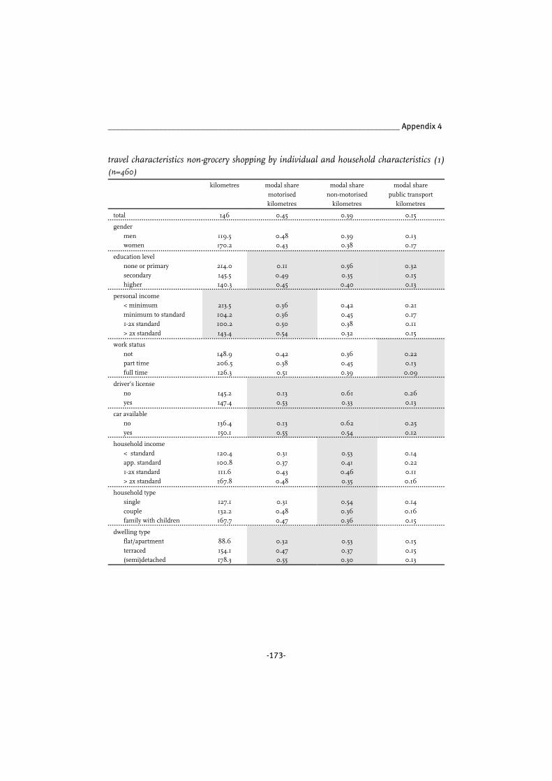
_____________________________________________________________________ Appendix 4
-173-
travel characteristics non-grocery shopping by individual and household characteristics (1)(n=460)
kilometres modal share
motorisedkilometres
modal share
non-motorisedkilometres
modal share
public transportkilometres
total 146 0.45 0.39 0.15
gender
menwomen
119.5170.2
0.480.43
0.390.38
0.130.17
education levelnone or primary
secondaryhigher
214.0
145.5140.3
0.11
0.490.45
0.56
0.350.40
0.32
0.150.13
personal income< minimum
minimum to standard1-2x standard
> 2x standard
213.5
104.2100.2
143.4
0.36
0.360.50
0.54
0.42
0.450.38
0.32
0.21
0.170.11
0.15
work status
notpart time
full time
148.9206.5
126.3
0.420.38
0.51
0.360.45
0.39
0.220.13
0.09
driver’s license
noyes
145.2147.4
0.130.53
0.610.33
0.260.13
car availableno
yes
136.4
150.1
0.13
0.55
0.62
0.54
0.25
0.12
household income
< standardapp. standard
1-2x standard> 2x standard
120.4100.8
111.6167.8
0.310.37
0.430.48
0.530.41
0.460.35
0.140.22
0.110.16
household typesingle
couplefamily with children
127.1
132.2167.7
0.31
0.480.47
0.54
0.360.36
0.14
0.160.15
dwelling typeflat/apartment
terraced(semi)detached
88.6
154.1178.3
0.32
0.470.55
0.53
0.370.30
0.15
0.150.13

Urban Form and Activity-Travel Patterns __________________________________________
-174-
travel characteristics non-grocery shopping by individual and household characteristics (2)(n=460)
trips modal share
motorised trips
modal share
non-motorisedtrips
modal share
public transporttrips
total 50.8 0.46 0.42 0.12
gender
menwomen
43.754.4
0.490.43
0.410.43
0.100.14
education levelnone or primary
secondaryhigher
84.4
52.041.6
0.12
0.500.46
0.60
0.390.44
0.28
0.110.10
personal income< minimum
minimum to standard1-2x standard
> 2x standard
63.5
56.441.1
40.7
0.36
0.330.49
0.57
0.46
0.550.43
0.32
0.18
0.110.09
0.11
work status
notpart time
full time
55.744.8
57.9
0.420.52
0.42
0.400.42
0.47
0.190.05
0.11
driver’s license
noyes
69.944.7
0.100.54
0.670.37
0.230.09
car availableno
yes
65.5
44.9
0.11
0.56
0.68
0.35
0.22
0.09
household income
< standardapp. standard
1-2x standard> 2x standard
62.252.8
52.345.8
0.330.36
0.460.48
0.600.44
0.450.39
0.080.20
0.090.13
household typesingle
couplefamily with children
51.4
47.852.0
0.30
0.500.48
0.62
0.370.40
0.09
0.130.12
dwelling typeflat/apartment
terraced(semi)detached
46.4
54.145.0
0.28
0.490.57
0.62
0.390.33
0.10
0.120.11

_____________________________________________________________________ Appendix 4
-175-
travel characteristics non-grocery shopping by spatial characteristics (1) (n=460)
kilometres modal sharemotorised
kilometres
modal sharenon-motorised
kilometres
modal sharepublic transport
kilometres
total 146 0.45 0.39 0.15
city typeconcentric
lobepoly-nuclear (Almere)
grid
157.2
150.8184.9
109.9
0.47
0.380.72
0.39
0.36
0.410.16
0.50
0.16
0.190.11
0.11
transportation network type
cityradial
ringgrid
144.5
170.7120.4
0.51
0.480.39
0.26
0.420.43
0.22
0.090.17
transportation network typeneighbourhood
ringloop
radialaxial
gridtangential
188.8110.1
151.8108.9
68.8137.4
0.530.60
0.300.39
0.380.52
0.330.28
0.540.35
0.520.39
0.130.13
0.140.25
0.100.09
local street network typeloop/grid
looploop/tree
gridtree
150.6
169.4141.7
135.552.4
0.65
0.520.43
0.200.39
0.23
0.330.32
0.710.49
0.12
0.140.24
0.060.12
mixed land useno
limitedample
136.6
161.193.0
0.45
0.490.24
0.38
0.350.67
0.24
0.220.06
shopping facilitiesnone or just a few
small nghbhd centrelarge nghbhd centre
city district centrecity centre
178.0
138.8169.6
70.993.0
0.67
0.410.48
0.170.24
0.24
0.420.33
0.530.67
0.09
0.160.17
0.310.10
locationinside Randstad
outside Randstad
119.0
163.8
0.52
0.41
0.37
0.41
0.11
0.17

Urban Form and Activity-Travel Patterns __________________________________________
-176-
travel characteristics non-grocery shopping by spatial characteristics (2) (n=460)
trips modal share
motorised trips
modal share
non-motorisedtrips
modal share
public transporttrips
total 50.8 0.46 0.42 0.12
city type
concentriclobe
poly-nuclear (Almere)grid
50.744.4
46.958.3
0.460.41
0.760.40
0.410.43
0.160.53
0.130.16
0.080.07
transportation network typecity
radialring
grid
49.252.4
50.0
0.540.48
0.40
0.280.46
0.47
0.180.06
0.13
transportation network type
neighbourhoodring
loopradial
axialgrid
tangential
50.9
49.736.4
59.540.9
59.3
0.54
0.590.34
0.410.35
0.49
0.36
0.320.55
0.390.57
0.46
0.10
0.090.12
0.200.08
0.06
local street network type
loop/gridloop
loop/treegrid
tree
49.355.6
42.041.2
77.5
0.650.53
0.440.19
0.44
0.260.37
0.330.77
0.49
0.090.10
0.220.04
0.07
mixed land use
nolimited
ample
52.549.1
53.6
0.490.51
0.17
0.410.38
0.76
0.130.12
0.07
shopping facilities
none or just a fewsmall nghbhd centre
large nghbhd centrecity district centre
city centre
54.948.0
51.154.3
53.6
0.680.44
0.470.17
0.17
0.270.42
0.400.63
0.76
0.060.14
0.130.20
0.07
location
inside Randstadoutside Randstad
48.856.9
0.520.42
0.410.43
0.070.14
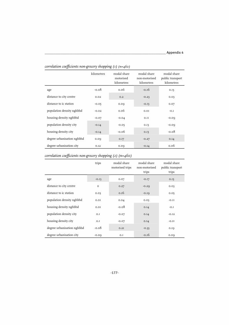
_____________________________________________________________________ Appendix 4
-177-
correlation coefficients non-grocery shopping (1) (n=460)
kilometres modal share
motorised
kilometres
modal share
non-motorised
kilometres
modal share
public transport
kilometres
age -0.08 0.06 -0.16 0.13
distance to city centre 0.02 0.2 -0.23 0.03
distance to ic station -0.05 0.09 -0.13 0.07
population density nghbhd -0.02 0.06 0.01 -0.1
housing density nghbhd -0.07 -0.04 0.11 -0.09
population density city -0.14 -0.05 0.13 -0.09
housing density city -0.14 -0.06 0.13 -0.08
degree urbanisation nghbhd 0.09 0.17 -0.27 0.14
degree urbanisation city 0.12 0.09 -0.14 0.06
correlation coefficients non-grocery shopping (2) (n=460)
trips modal share
motorised trips
modal share
non-motorised
trips
modal share
public transport
trips
age -0.13 0.07 -0.17 0.15
distance to city centre 0 0.27 -0.29 0.03
distance to ic station 0.03 0.16 -0.19 0.05
population density nghbhd 0.01 0.04 0.03 -0.11
housing density nghbhd 0.01 -0.08 0.14 -0.1
population density city 0.1 -0.07 0.14 -0.12
housing density city 0.1 -0.07 0.14 -0.11
degree urbanisation nghbhd -0.08 0.21 -0.33 0.19
degree urbanisation city -0.09 0.1 -0.16 0.09

Urban Form and Activity-Travel Patterns __________________________________________
-178-
travel characteristics recurring leisure activities by individual and household characteristics(n=340)
kilometres modal sharemotorised kilometres
trips modal share motorisedtrips
total 24.2 0.58 6.2 0.55
gender
menwomen
25.626.2
0.610.54
6.75.9
0.580.52
education levelnone or primary
secondaryhigher
23.2
20.533.0
0.49
0.610.54
6.8
6.06.3
0.45
0.600.50
personal income < minimum
minimum to standard1-2x standard
> 2x standard
27.4
16.820.9
28.2
0.55
0.530.58
0.65
6.8
5.65.8
6.2
0.51
0.510.56
0.65
work status
notpart time
full time
23.525.6
25.1
0.580.50
0.61
6.85.5
6.0
0.570.45
0.58
driver’s license
noyes
22.026.9
0.300.64
7.26.0
0.270.61
car availableno
yes
21.3
27.2
0.32
0.64
7.4
5.9
0.28
0.62
household income
< standardapp. standard
1-2x standard> 2x standard
12.724.2
8.633.0
0.500.63
0.550.58
6.06.1
5.66.3
0.520.58
0.560.55
household typesingle
couplefamily with children
21.7
28.322.5
0.60
0.650.53
6.5
6.55.8
0.55
0.620.51
dwelling typeflat/apartment
terraced(semi)detached
18.2
21.438.1
0.47
0.610.60
6.6
6.16.3
0.38
0.600.58

_____________________________________________________________________ Appendix 4
-179-
travel characteristics recurring leisure activities by spatial characteristics (n=340)
kilometres modal sharemotorised kilometres
trips modal sharemotorised trips
total 24.2 0.58 6.2 0.55
city type
concentriclobe
poly-nuclear (Almere)grid
27.535.5
11.512.9
0.610.59
0.640.51
6.06.2
5.26.7
0.570.56
0.640.50
transportation network typecity
radialring
grid
16.230.1
23.1
0.700.49
0.60
5.76.5
6.2
0.660.47
0.57
transportation network type
neighbourhoodring
loopradial
axialgrid
tangential
23.2
11.341.0
15.29.5
21.4
0.54
0.740.53
0.650.36
0.66
6.4
5.56.4
6.24.4
6.0
0.51
0.800.47
0.630.31
0.63
local street network type
loop/gridloop
loop/treegrid
tree
15.627.0
13.942.2
13.8
0.630.60
0.670.36
0.61
5.13.5
5.96.6
6.5
0.640.56
0.630.34
0.61
mixed land use
nolimited
ample
29.922.8
12.8
0.630.59
0.29
5.96.4
5.8
0.650.54
0.26
sports facilities
not available locallyavailable locally
45.120.5
0.310.62
6.26.2
0.330.60
locationinside Randstad
outside Randstad
15.9
29.0
0.61
0.57
5.9
6.4
0.59
0.53

Urban Form and Activity-Travel Patterns __________________________________________
-180-
correlation coefficients recurring leisure activities (n=340)
kilometres modal share
motorised
kilometres
trips modal share
motorised trips
age -0.09 0.14 0 0.19
distance to city centre -0.06 0.21 -0.03 0.2
distance to ic station -0.06 0.17 -0.02 0.16
population density nghbhd -0.02 -0.01 -0.05 0
housing density nghbhd -0.02 -0.05 -0.02 -0.04
population density city -0.04 0.01 0 0.03
housing density city -0.04 0 0 0.02
degree urbanisation nghbhd -0.1 0.13 -0.08 0.12
degree urbanisation city 0.04 0 -0.04 -0.01

_____________________________________________________________________ Appendix 4
-181-
travel characteristics home-to-work by individual and household characteristics (1) (n=200)
kilometres modal sharemotorised
kilometres)
modal sharenon-motorised
kilometres
modal sharepublic transport
kilometres
total 224.6 0.46 0.41 0.13
gendermen
women
303.3
160.0
0.49
0.44
0.36
0.47
0.16
0.10
education level
none or primarysecondary
higher
36.1148.9
288.7
0.000.41
0.51
1.000.47
0.36
0.000.12
0.13
personal income
< minimumminimum to standard
1-2x standard> 2x standard
55.191.2
211.7400.1
0.180.38
0.390.66
0.790.55
0.470.17
0.030.07
0.140.16
work statuspart time
full time
89.8
277.7
0.42
0.48
0.50
0.38
0.09
0.14
driver’s license
noyes
88.1236.3
0.000.51
0.770.38
0.230.11
car availableno
yes
103.1
240.5
0.00
0.54
0.80
0.35
0.19
0.11
household income
< standardapp. standard
1-2x standard> 2x standard
81.0161.4
229.5253.9
0.310.57
0.550.46
0.640.32
0.390.40
0.050.11
0.060.14
household typesingle
couplefamily with children
233.5
312.4162.8
0.55
0.520.36
0.38
0.360.48
0.07
0.120.16
dwelling typeflat/apartment
terraced(semi)detached
152.3
225.7344.2
0.45
0.430.55
0.51
0.420.25
0.04
0.150.19

Urban Form and Activity-Travel Patterns __________________________________________
-182-
travel characteristics home-to-work by individual and household characteristics (2) (n = 200)
trips modal share
motorised trips
modal share
non-motorisedtrips
modal share
public transporttrips
total 15.7 0.45 0.42 0.13
gender
menwomen
15.915.6
0.490.41
0.340.50
0.170.10
education levelnone or primary
secondaryhigher
7.2
15.416.4
0.00
0.410.49
1.00
0.470.38
0.00
0.130.13
personal income< minimum
minimum to standard1-2x standard
> 2x standard
8.1
15.617.1
17.8
0.13
0.400.39
0.68
0.76
0.540.45
0.16
0.11
0.070.16
0.15
work status
part timefull time
11.517.3
0.360.49
0.530.37
0.140.11
driver’s licenseno
yes
15.1
15.8
0.00
0.50
0.77
0.39
0.23
0.11
car available
noyes
15.115.8
0.000.53
0.770.37
0.230.10
household income< standard
app. standard1-2x standard
> 2x standard
17.1
12.116.9
15.7
0.35
0.450.52
0.46
0.57
0.480.35
0.41
0.08
0.080.13
0.13
household type
singlecouple
family with children
17.015.4
15.1
0.530.54
0.35
0.360.35
0.50
0.110.11
0.15
dwelling type
flat/apartmentterraced
(semi)detached
18.315.3
13.0
0.470.40
0.56
0.460.45
0.29
0.060.15
0.15

_____________________________________________________________________ Appendix 4
-183-
travel characteristics home-to-work by spatial characteristics (1) (n=200)
kilometres modal sharemotorised
kilometres
modal sharenon-motorised
kilometres
modal sharepublic transport
kilometres
total 224.6 0.46 0.41 0.13
city typeconcentric
lobepoly-nuclear (Almere)
grid
159.9
226.4326.8
228.3
0.40
0.380.53
0.54
0.50
0.530.17
0.36
0.10
0.100.31
0.09
transportation network type
cityradial
ringgrid
164.0
318.5140.6
0.38
0.430.54
0.54
0.370.38
0.08
0.180.08
transportation network typeneighbourhood
ringloop
radialaxial
gridtangential
298.0271.6
221.9166.4
61.2183.9
0.480.42
0.380.63
0.500.35
0.380.27
0.560.31
0.470.43
0.150.31
0.060.06
0.030.22
local street network typeloop/grid
looploop/tree
gridtree
294.9
269.4144.3
204.2123.2
0.47
0.480.46
0.320.77
0.26
0.400.50
0.560.18
0.27
0.130.04
0.120.04
mixed land useno
limitedample
195.8
265.9103.0
0.45
0.500.29
0.43
0.360.66
0.12
0.150.04
locationinside Randstad
outside Randstad
191.9
254.0
0.52
0.41
0.30
0.51
0.18
0.08

Urban Form and Activity-Travel Patterns __________________________________________
-184-
travel characteristics home-to-work by spatial characteristics (2) (n=200)
trips modal share
motorised trips
modal share
non-motorised trips
modal share
public transporttrips
total 15.7 0.45 0.42 0.13
city type
concentriclobe
poly-nuclear (Almere)grid
14.416.9
15.216.2
0.410.39
0.470.54
0.500.52
0.190.37
0.090.09
0.350.09
transportation network typecity
radialring
grid
17.616.4
14.2
0.400.42
0.52
0.500.40
0.41
0.100.19
0.07
transportation network type
neighbourhoodring
loopradial
axialgrid
tangential
15.9
14.413.9
17.715.8
17.8
0.47
0.410.39
0.600.54
0.36
0.39
0.220.55
0.350.41
0.43
0.14
0.380.06
0.050.05
0.21
local street network type
loop/gridloop
loop/treegrid
tree
15.617.4
12.615.7
16.6
0.420.48
0.470.35
0.67
0.270.40
0.500.52
0.29
0.310.12
0.030.13
0.03
mixed land use
nolimited
ample
15.615.6
17.0
0.440.48
0.34
0.420.39
0.61
0.140.13
0.06
location
inside Randstadoutside Randstad
15.915.5
0.500.42
0.310.51
0.190.08

_____________________________________________________________________ Appendix 4
-185-
correlation coefficients home-to-work (1) (n=200)
kilometres modal share
motorisedkilometres
modal share
non-motorisedkilometres
modal share
public transportkilometres
age -0.15 0.06 -0.04 -0.03
distance to city centre 0.06 0.14 -0.15 0.02
distance to ic station 0.03 0.14 -0.11 -0.04
employment 0.05 -0.05 0.2 -0.2
population density nghbhd -0.04 -0.14 0.08 0.09
housing density nghbhd -0.05 -0.12 0.08 0.06
population density city -0.16 0.1 -0.06 -0.06
housing density city -0.16 0.11 -0.06 -0.07
degree urbanisation nghbhd 0.1 -0.03 0.01 0.03
degree urbanisation city 0.12 -0.05 -0.03 0.1
correlation coefficients home-to-work (2) (n=200)
trips modal share
motorised trips
modal share
non-motorisedtrips
modal share
public transporttrips
age -0.21 -0.01 0.03 -0.03
distance to city centre -0.07 0.07 -0.11 0.05
distance to ic station -0.5 0.07 -0.07 -0.01
employment 0.09 -0.02 0.19 -0.24
population density nghbhd 0.05 -0.08 0 0.12
housing density nghbhd 0.09 -0.06 0.01 0.08
population density city 0.07 0.1 -0.06 -0.07
housing density city 0.06 0.11 -0.06 -0.08
degree urbanisation nghbhd -0.16 -0.04 0.03 0.02
degree urbanisation city -0.13 -0.07 0 0.1

-186-
APPENDIX 5 | Multilevel Analyses Frequent Activities
The tables listed below report the results from the multilevel analyses on frequent
activity data, as discussed in chapter 6. The analyses reported in this appendix are based
on data on grocery shopping trips from 392 respondents, on non-grocery shopping trips
from 460 respondents, on recurring leisure trips from 340 respondents and on home-to-
work trips from 200 respondents.
Parameters reported in bold face type are significant at the 5% level, parameters reported
in italics are significant at the 10% level. The tables report parameter values and t-values,
as is usual when reporting multilevel analysis results.
In the tables the following abbreviations are used for layout reasons:
TNTC = transportation network type city
TNTN = transportation network type neighbourhood
LSNT = local street network type

______________________________________________________________________ Appendix 5
-187-
total number of kilometres grocery shopping
null model best model
fixed part
individual effect
intercept
average distance
random part
individual
group
slope average distance
22.377 (7.289)
12712.8
5.4
24.496 (3.424)9.017 (2.007)
435.7
70.3
28.5
individualR2groupR2
0.915
0.915
intra class correlation = 0.0%
total number of motorised kilometres grocery shopping
null model best model
fixed part
individual effects
intercept
average distance
random part
individual
group
slope average distance
11.228 (5.855)
8157.8
6.0
13.704 (2.618)5.812 (1.488)
58.7
78.1
25.5
individualR2groupR2
0.809
0.780
intra class correlation = 0.1%
total number of non-motorised kilometres grocery shopping
null model best model
fixed part
individual effects
intercept
average distance
working part time
working full time
11.119 (4.491) 12.308 (3.323)3.681 (2.116)
2.540 (2.281)
-5.883 (1.827)

Urban Form and Activity-Travel Patterns __________________________________________
-188-
random part
individual
group
slope average distance
4747.9
6.7
406.1
60.6
37.0
individualR2groupR2
0.160
0.169
intra class correlation = 0.1%
modal split kilometres grocery shopping
null model best model
fixed part
individual effects
intercept
car available
working part time
working full time
group effects
TNTN ring
TNTN loop
TNTN radial
TNTN axial
TNTN grid
degree of urbanisation neighbourhood
interaction effects
car * none or just a few shops
car * small neighb. shopping centre
car * large neighb. shopping centre
car * city district shopping centre
part time* none or just a few shops
part time * small neighb. shopping centre
part time * large neighb. shopping centre
part time * city district shopping centre
full time * none or just a few shops
full time * small neighb. shopping centre
full time * large neighb. shopping centre
full time * city district shopping centre
random part
individual
group
38.208 (4.229)
1786.0
171.2
24.871 (4.156)14.220 (4.021)
-5.293 (6.119)8.845 (4.785)
2.610 (6.345)
26.579 (8.796)
-12.161 (7.189)
0.927 (7.692)
-13.749 (11.817)6.093 (3.197)
16.550 (6.910)
3.703 (5.106)
1.321 (5.793)
-9.982 (11.076)
6.174 (9.591)
-1.728 (7.819)
-26.346 (8.762)
23.534 (16.285)
-2.427 (8.010)
1.529 (6.352)
20.148 (7.677)
-13.693 (13.821)
1436.00
59.74

______________________________________________________________________ Appendix 5
-189-
individualR2groupR2
0.236
0.441
intra class correlation = 8.7%
Results given are for share of motorised kilometres. Parameters for non-motorised
kilometres are identical, but with opposite sign and intercept = 75.129 (4.156).
total number of trips grocery shopping
null model best model
fixed part
individual effects
intercept
age
personal income over standard
working part time
working full time
group effects
location in Randstad
random part
individual
group
14.511 (0.682)
90.1
1.3
16.271 (0.992)0.149 (0.048)-1.308 (0.641)
0.016 (0.971)
-2.652 (0.967)
-3.402 (1.479)
69.9
3.8
individualR2groupR2
0.194
0.000
intra class correlation = 1.4%
total number of motorised trips grocery shopping
null model best model
fixed part
individual effects
intercept
secondary education
higher education
car available
single family dwelling
3.826 (0.482) 1.417 (0.689)1.166 (0.637)
0.079 (0.662)
1.702 (0.431)0.846 (0.469)

Urban Form and Activity-Travel Patterns __________________________________________
-190-
group effects
none or just a few shops
small neighbourhood shopping centre
large neighbourhood shopping centre
city district shopping centre
random part
individual
group
30.4
1.7
0.228 (0.823)
0.050 (0.643)
2.303 (0.731)
-1.448 (1.333)
27.9
0.0
individualR2groupR2
0.129
0.501
intra class correlation = 5.3%
total number of non-motorised trips grocery shopping
null model best model
fixed part
individual effects
intercept
car available
working part time
working full time
group effects
none or just a few shops
small neighbourhood shopping centre
large neighbourhood shopping centre
city district shopping centre
interaction effects
part time* none or just a few shops
part time * small neighb. centre
part time * large neighb. centre
part time * city district shopping centre
random part
individual
group
10.673 (0.813)
107.4
3.2
13.959 (0.952)-2.305 (0.744)
-0.932 (1.398)
-4.281 (0.853)
-4.457 (1.434)
-0.542 (1.161)
-3.622 (1.380)5.744 (2.435)
0.788 (1.985)
1.481 (1.589)
4.103 (1.743)-10.098 (3.453)
84.4
0.8
individualR2groupR2
0.230
0.389
intra class correlation = 2.9%

______________________________________________________________________ Appendix 5
-191-
modal split trips grocery shopping
null model best model
fixed part
individual effects
intercept
personal income minimum to standard
personal income standard to 2x standard
personal income over 2x standard
car available
working part time
working full time
group effects
TNTN ring
TNTN loop
TNTN radial
TNTN axial
TNTN grid
interaction effects
car* none or just a few shops
car * small neighb. shopping centre
car * large neighb. shopping centre
car * city district shopping centre
part time* LSNT loop/grid
part time * LSNT loop
part time * LSNT loop/tree
part time * LSNT grid
part time* none or just a few shops
part time * small neighb. shopping centre
part time * large neighb. shopping centre
part time * city district shopping centre
full time* TNTN ring
full time* TNTN loop
full time* TNTN radial
full time* TNTN axial
full time* TNTN grid
random part
individual
group
34.221 (3.771)
1697.5
114.6
22.628 (3.857)
-2.730 (4.303)
-3.766 (4.341)
14.343 (4.536)11.269 (3.846)
-2.716 (6.671)
5.727 (4.265)
1.524 (5.721)
25.730 (8.190)
-5.300 (6.510)
-2.012 (7.073)
-10.906 (10.872)
15.605 (6.271)
3.173 (4.679)
6.837 (5.330)
-8.744 (9.855)-27.142 (14.521)
6.545 (7.957)
8.934 (7.796)
12.854 (9.310)20.388 (12.000)
-6.909 (9.434)
-32.192 (9.173)
9.689 (15.502)
17.307 (6.104)
8.831 (8.496)
0.429 (6.016)
-5.336 (7.565)
-13.644 (12.455)
1315.7
39.7

Urban Form and Activity-Travel Patterns __________________________________________
-192-
individualR2groupR2
0.252
0.446
intra class correlation = 6.3%
Results given are for share of motorised trips. Parameters for non-motorised trips are
identical, but with opposite sign and intercept = 77.372 (3.857).
total number of kilometres other shopping
null model best model
fixed part
individual effects
intercept
average distance
group effects
degree of urbanisation neighbourhood
random part
individual
group
slope average distance
145.622 (14.568)
74197.1
78.9
150.831 (18.781)23.740 (6.745)
22.190 (10.864)
23907.2
3488.9
484.4
individualR2groupR2
0.327
0.269
intra class correlation = 0.1%
total number of motorised kilometres other shopping
null model best model
fixed part
individual effects
intercept
sometimes car available
always car available
average distance
interaction effects
always car * TNTC radial
always car * TNTC ring
64.403 (9.432) 38.666 (14.879)47.970 (13.409)
31.493 (15.508)13.042 (4.400)
0.985 (21.967)
49.381 (18.515)

______________________________________________________________________ Appendix 5
-193-
random part
individual
group
slope average distance
14580.1
625.2
6171.7
1744.4
234.9
individualR2groupR2
0.402
0.234
intra class correlation = 4.1%
total number of non-motorised kilometres other shopping
null model best model
fixed part
individual effects
intercept
age
average distance
working part time
working full time
random part
individual
group
slope average distance
51.719 (13.150)
51428.7
21.1
66.515 (11.733)-1.276 (0.406)
7.187 (3.813)
-23.523 (19.308)
-32.824 (14.609)
10775.0
126.3
149.3
individualR2groupR2
0.147
0.148
intra class correlation = 0.0%
total number of public transport kilometres other shopping
null model best model
fixed part
individual effects
intercept
secondary education
higher education
random part
individual
group
27.557 (5.483)
8907.3
5.3
56.567 (20.550)-31.989 (21.950)
-24.187 (22.125)
8857.8
4.9
individualR2groupR2
0.006
0.006
intra class correlation = 0.1%

Urban Form and Activity-Travel Patterns __________________________________________
-194-
modal share motorised kilometres other shopping
null model best model
fixed part
individual effects
intercept
car available
terraced dwelling
(semi)detached dwelling
group effects
distance to city centre
TNTN ring
TNTN loop
TNTN radial
TNTN axial
TNTN grid
random part
individual
group
46.851 (5.069)
1763.0
338.3
18.414 (9.259)
39.828 (5.474)
8.850 (6.715)
17.230 (7.603)
4.624 (2.003)
-4.679 (7.306)
-0.937 (11.137)
-38.267 (7.913)-18.181 (7.819)
-1.336 (15.119)
1525.9
0.8
individualR2groupR2
0.273
0.757
intra class correlation = 16.1%
modal share non-motorised kilometres other shopping
null model best model
fixed part
individual effects
intercept
age
car available
multi person household
group effects
LSNT loop/grid
LSNT loop
LSNT loop/tree
LSNT grid
38.359 (5.071) 80.671 (11.664)-0.408 (0.157)
-24.263 (5.476)-13.045 (6.584)
-25.711 (11.437)-24.285 (10.334)
-13.388 (10.643)
14.959 (11.447)

______________________________________________________________________ Appendix 5
-195-
random part
individual
group
1617.8
349.3
1474.6
23.1
individualR2groupR2
0.239
0.717
intra class correlation = 17.8%
modal share public transport kilometres other shopping
null model best model
fixed part
individual effects
intercept
secondary education
higher education
car available
group effects
none or just a few shops
small neighbourhood shopping centre
large neighbourhood shopping centre
city district shopping centre
degree of urbanisation neighbourhood
interaction effects
secondary education * TNTN ring
secondary education * TNTN loop
secondary education * TNTN radial
secondary education * TNTN axial
secondary education * TNTN grid
car available * none/few shops
car available * small neighb. centre
car available * large neighb. centre
car available * city district centre
car available * degree urbanisation nghb
random part
individual
group
slope secondary education
slope higher education
slope car available
14.916 (2.308)
1005.5
29.5
19.765 (21.618)
8.427 (13.248)
0.817 (13.743)
-7.612 (21.576)
-1.271 (23.142)
6.452 (21.894)
47.983 (21.584)
-7.373 (24.568)
13.548 (4.654)
-9.921 (8.011)
-25.338 (11.270)
-12.337 (9.099)
4.726 (9.049)
-13.802 (21.059)
-2.428 (26.866)
-8.597 (25.088)-51.426 (25.121)
34.457 (29.594)-10.327 (5.488)
818.3
41.2
931.0
1667.7
1240.0

Urban Form and Activity-Travel Patterns __________________________________________
-196-
individualR2groupR2
0.091
0.330
intra class correlation = 2.9%
total number of trips other shopping
null model best model
fixed part
individual effects
intercept
sometimes car available
always car available
group effects
TNTN ring
TNTN loop
TNTN radial
TNTN axial
TNTN grid
random part
individual
group
slope sometimes car available
slope always car available
48.780 (2.947)
1905.6
34.6
67.738 (9.801)-16.494 (8.822)
-12.856 (9.058)
-4.180 (9.205)
-0.758 (12.758)-19.026 (10.090)
-8.773 (10.019)
-23.890 (16.747)
1778.3
341.2
414.3
621.2
individualR2groupR2
0.018
0.040
intra class correlation = 1.8%
total number of motorised trips other shopping
null model best model
fixed part
individual effects
intercept
car available
single family dwelling
19.976 (3.259) 7.140 (6.044)
19.160 (3.615)11.109 (4.183)
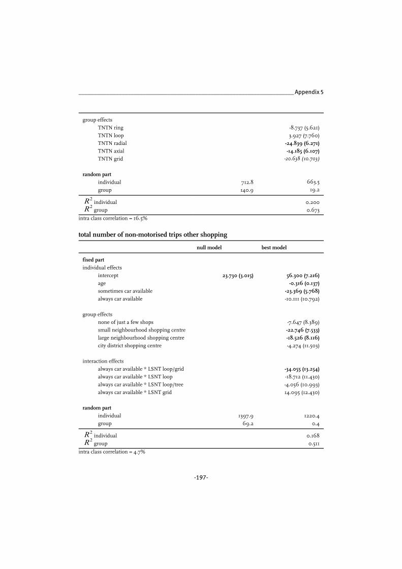
______________________________________________________________________ Appendix 5
-197-
group effects
TNTN ring
TNTN loop
TNTN radial
TNTN axial
TNTN grid
random part
individual
group
712.8
140.9
-8.737 (5.621)
3.927 (7.760)
-24.839 (6.271)-14.185 (6.107)
-20.638 (10.703)
663.5
19.2
individualR2groupR2
0.200
0.673
intra class correlation = 16.5%
total number of non-motorised trips other shopping
null model best model
fixed part
individual effects
intercept
age
sometimes car available
always car available
group effects
none of just a few shops
small neighbourhood shopping centre
large neighbourhood shopping centre
city district shopping centre
interaction effects
always car available * LSNT loop/grid
always car available * LSNT loop
always car available * LSNT loop/tree
always car available * LSNT grid
random part
individual
group
23.730 (3.015)
1397.9
69.2
56.300 (7.216)-0.316 (0.137)
-23.369 (5.768)
-10.111 (10.792)
-7.647 (8.389)
-22.746 (7.533)-18.526 (8.116)
-4.274 (11.503)
-34.055 (13.254)
-18.712 (11.430)
-4.056 (10.993)
14.095 (12.430)
1220.4
0.4
individualR2groupR2
0.168
0.511
intra class correlation = 4.7%

Urban Form and Activity-Travel Patterns __________________________________________
-198-
total number of public transport trips other shopping
null model best model
fixed part
individual effects
intercept
age
car available
group effects
degree of urbanisation neighbourhood
interaction effects
age * degree urbanisation neighb.
car available * degree urbanisation nghb
random part
individual
group
slope car available
5.504 (1.538)
415.0
15.1
14.221 (3.287)0.147 (0.070)
-11.299 (3.647)
11.425 (2.973)
0.168 (0.058)-10.240 (3.295)
352.873.486.4
individualR2groupR2
0.149
0.443
intra class correlation = 3.5%
modal share of motorised trips other shopping
null model best model
fixed part
individual effects
intercept
car available
single family dwelling
working part time
working full time
group effects
distance to city centre
random part
individual
group
45.525 (5.490)
1723.1
422.4
4.281 (7.999)
34.799 (5.621)13.883 (6.837)
-3.918 (6.883)9.371 (5.136)
7.404 (2.798)
1460.0
187.2

______________________________________________________________________ Appendix 5
-199-
individualR2groupR2
0.232
0.475
intra class correlation = 19.7%
modal share non-motorised trips other shopping
null model best model
fixed part
individual effects
intercept
age
car available
multi person household
group effects
distance to city centre
interaction effects
age * degree urbanisation neighb.
random part
individual
group
43.605 (5.873)
1592.9
512.9
72.126 (7.502)-0.286 (0.161)
-20.050 (5.565)-15.734 (6.609)
-9.811 (2.710)
-0.261 (0.127)
1451.0
188.0
individualR2groupR2
0.222
0.545
intra class correlation = 24.4%
modal share public transport trips other shopping
null model best model
fixed part
individual effects
intercept
car available
working part time
working full time
group effects
LSNT loop/grid
LSNT loop
LSNT loop/tree
LSNT grid
11.748 (2.441) 25.177 (7.125)-12.341 (4.869)
-7.156 (4.896)
-11.503 (3.683)
1.011 (7.100)
5.073 (6.404)
15.086 (6.578)
-5.477 (7.043)
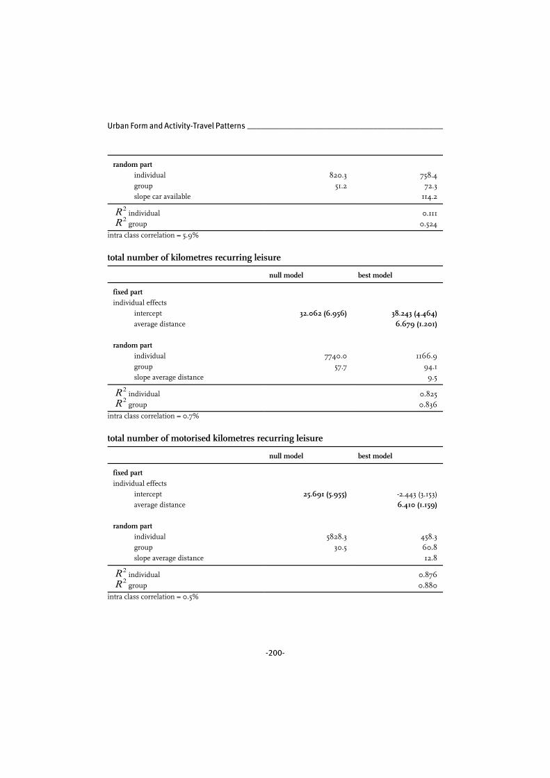
Urban Form and Activity-Travel Patterns __________________________________________
-200-
random part
individual
group
slope car available
820.3
51.2
758.4
72.3
114.2
individualR2groupR2
0.111
0.524
intra class correlation = 5.9%
total number of kilometres recurring leisure
null model best model
fixed part
individual effects
intercept
average distance
random part
individual
group
slope average distance
32.062 (6.956)
7740.0
57.7
38.243 (4.464)6.679 (1.201)
1166.9
94.1
9.5
individualR2groupR2
0.825
0.836
intra class correlation = 0.7%
total number of motorised kilometres recurring leisure
null model best model
fixed part
individual effects
intercept
average distance
random part
individual
group
slope average distance
25.691 (5.955)
5828.3
30.5
-2.443 (3.153)
6.410 (1.159)
458.3
60.8
12.8
individualR2groupR2
0.876
0.880
intra class correlation = 0.5%
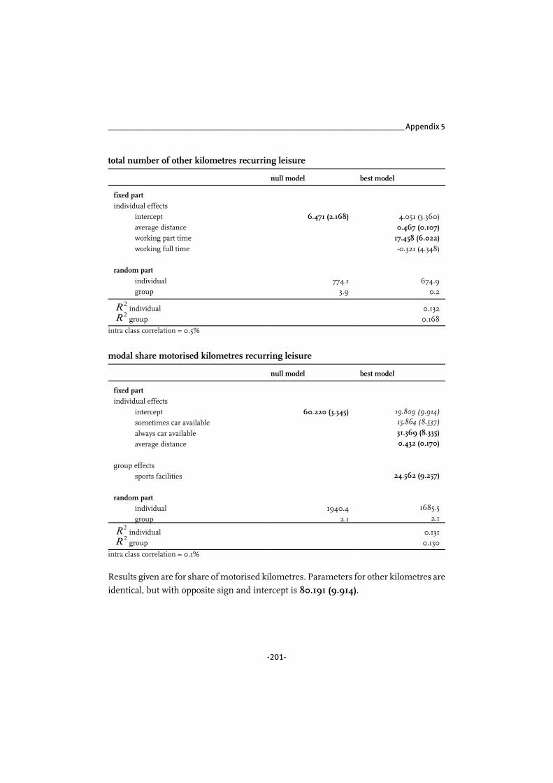
______________________________________________________________________ Appendix 5
-201-
total number of other kilometres recurring leisure
null model best model
fixed part
individual effects
intercept
average distance
working part time
working full time
random part
individual
group
6.471 (2.168)
774.1
3.9
4.051 (3.360)
0.467 (0.107)17.458 (6.022)
-0.321 (4.348)
674.9
0.2
individualR2groupR2
0.132
0.168
intra class correlation = 0.5%
modal share motorised kilometres recurring leisure
null model best model
fixed part
individual effects
intercept
sometimes car available
always car available
average distance
group effects
sports facilities
random part
individual
group
60.220 (3.345)
1940.4
2.1
19.809 (9.914)15.864 (8.537)
31.369 (8.335)0.432 (0.170)
24.562 (9.257)
1685.5
2.1
individualR2groupR2
0.131
0.130
intra class correlation = 0.1%
Results given are for share of motorised kilometres. Parameters for other kilometres are
identical, but with opposite sign and intercept is 80.191 (9.914).

Urban Form and Activity-Travel Patterns __________________________________________
-202-
total number of trips recurring leisure
null model best model
fixed part
individual effects
intercept
gender
sometimes car available
always car available
terraced dwelling
(semi)detached dwelling
random part
individual
group
6.431 (0.288)
14.5
0.01
8.857 (0.891)-1.342 (0.576)-1.464 (0.784)
-0.966 (0.764)
-0.681 (0.715)
-1.838 (0.864)
13.9.5
0.01
individualR2groupR2
0.043
0.042
intra class correlation = 0.1%
total number of motorised trips recurring leisure
null model best model
fixed part
individual effects
intercept
sometimes car available
always car available
working part time
working full time
group effects
sports facilities
random part
individual
group
3.615 (0.265)
12.2
0.01
1.236 (0.861)
0.671 (0.688)
2.306 (0.662)-1.998 (0.754)
0.105 (0.561)
1.617 (0.732)
10.5
0.01
individualR2groupR2
0.142
0.148
intra class correlation = 0.2%

______________________________________________________________________ Appendix 5
-203-
total number of other trips recurring leisure
null model best model
fixed part
individual effects
intercept
sometimes car available
always car available
group effects
sports facilities
random part
individual
group
2.770 (0.377)
13.4
1.0
6.647 (0.841)-2.127 (0.727)-3.042 (0.711)
-2.034 (0.781)
12.3
0.0
individualR2groupR2
0.144
0.470
intra class correlation = 6.9%
modal share motorised trips recurring leisure
null model best model
fixed part
individual effects
intercept
sometimes car available
always car available
single family dwelling
average distance
working part time
working full time
random part
individual
group
57.421 (3.307)
1908.5
1.2
29.557 (9.087)15.342 (8.570)
34.167 (8.124)19.140 (7.540)0.369 (0.166)
-24.877 (9.420)
-6.903 (6.866)
1606.8
4.3
individualR2groupR2
0.156
0.142
intra class correlation = 0.1%
Results given are for share of motorised trips. Parameters for other trips are identical,
but with opposite sign and intercept is 70.443 (9.087).

Urban Form and Activity-Travel Patterns __________________________________________
-204-
total number of kilometres home-to-work
null model best model
fixed part
individual effects
intercept
average distance
random part
individual
group
slope average distance
237.340 (43.302)
203999.4
4194.4
245.631 (13.157)17.058 (1.723)
4450.3
1699.7
42.9
individualR2groupR2
0.784
0.757
intra class correlation = 2.0%
total number of motorised kilometres home-to-work
null model best model
fixed part
individual effects
intercept
household with children
average distance
random part
individual
group
slope average distance
153.972 (41.648)
175060.7
5547.1
163.131 (23.244)-19.724 (11.338)
12.576 (2.462)
13580.6
5368.2
76.7
individualR2groupR2
0.508
0.349
intra class correlation = 3.1%

______________________________________________________________________ Appendix 5
-205-
total number of non-motorised kilometres home-to-work
null model best model
fixed part
individual effects
intercept
personal income minimum to standard
personal income standard to 2x standard
personal income 2x standard and over
car available
group effects
TNTC radial
TNTC ring
random part
individual
group
23.158 (4.141)
2115.1
9.1
41.617 (6.393)-12.601 (7.093)
2.626 (7.018)
-10.304 (6.966)
-12.910 (5.619)
19.868 (6.907)
-10.127 (5.552)
1933.0
4.1
individualR2groupR2
0.088
0.099
intra class correlation = 0.4%
total number of public transport kilometres home-to-work
null model best model
fixed part
individual effects
intercept
multi person household
average distance
interaction effects
multi person * TNTC radial
multi person * TNTC ring
average distance * TNTC radial
average distance * TNTC ring
random part
individual
group
slope average distance
59.719 (27.876)
44317.7
7052.2
31.578 (18.714)22.071 (11.892)
2.786 (1.631)
-22.280 (18.095)
54.337 (15.193)
-1.751 (1.632)2.965 (1.408)
11482.9
2671.7
26.6
individualR2groupR2
0.310
0.213
intra class correlation = 13.7%

Urban Form and Activity-Travel Patterns __________________________________________
-206-
modal share motorised kilometres home-to-work
null model best model
fixed part
individual effects
intercept
secondary education
higher education
sometimes car available
always car available
average distance
group effects
LSNT loop/grid
LSNT loop
LSNT loop/tree
LSNT grid
random part
individual
group
44.462 (4.704)
1924.8
109.7
13.552 (10.005)16.728 (9.925)
24.034 (9.675)
2.191 (5.547)
30.482 (5.165)0.357 (0.156)
-22.749 (7.719)
-1.106 (5.996)
6.654 (7.405)
-5.715 (6.846)
1397.6
2.2
individualR2groupR2
0.312
0.461
intra class correlation = 5.4%
modal share non-motorised kilometres home-to-work
null model best model
fixed part
individual effects
intercept
secondary education
higher education
personal income minimum to standard
personal income standard to 2x standard
personal income over 2x standard
sometimes car available
always car available
average distance
42.728 (4.740) 73.277 (9.564)-17.399 (9.443)
-14.736 (9.908)
-2.132 (6.033)
0.393 (5.879)
-19.614 (6.329)
-6.522 (5.317)
-22.084 (5.105)-0.568 (0.153)

______________________________________________________________________ Appendix 5
-207-
random part
individual
group
1881.1
120.9
1276.2
58.5
individualR2groupR2
0.333
0.378
intra class correlation = 6.0%
modal share public transport kilometres home-to-work
null model best model
fixed part
individual effects
intercept
average distance
group effects
concentric city
lobe city
poly-nuclear city (Almere)
TNTN ring
TNTN loop
TNTN radial
TNTN axial
TNTN grid
random part
individual
group
12.833 (3.740)
879.6
115.1
19.939 (3.161)0.229 (0.119)
-5.526 (5.955)
-1.322 (5.220)
22.484 (6.742)
-4.028 (5.083)17.043 (8.324)
-9.384 (6.618)
-2.881 (6.057)
1.524 (8.590)
813.7
0.5
individualR2groupR2
0.181
0.491
intra class correlation = 11.6%
total number of trips home-to-work
null model best model
fixed part
individual effects
intercept
personal income above average
couple
family with children
working full time
17.141 (0.590) 16.280 (0.628)1.216 (0.533)-1.123 (0.663)
0.291 (0.652)
2.590 (0.583)

Urban Form and Activity-Travel Patterns __________________________________________
-208-
group effects
TNTC radial
TNTC ring
random part
individual
group
35.7
1.0
1.734 (0.918)
-0.096 (0.768)
24.7
1.6
individualR2groupR2
0.284
0.150
intra class correlation = 2.7%
total number of motorised trips home-to-work
null model best model
fixed part
individual effects
intercept
personal income (minimum to standard)
personal income (standard to 2x standard)
personal income (over 2x standard)
sometimes car available
always car available
average distance
group effects
LSNT loop/grid
LSNT loop
LSNT loop/tree
LSNT grid
random part
individual
group
7.786 (0.895)
75.2
3.3
4.803 (0.976)
0.440 (1.232)
-0.454 (1.237)
3.193 (1.243)
-0.564 (1.109)
5.242 (1.055)0.069 (0.032)
-3.831 (1.576)
1.448 (1.152)
-0.385 (1.466)
-0.401 (1.335)
55.1
0.1
individualR2groupR2
0.297
0.443
intra class correlation = 4.2%

______________________________________________________________________ Appendix 5
-209-
total number of non-motorised trips home-to-work
null model best model
fixed part
individual effects
intercept
personal income minimum to standard
personal income standard to 2x standard
personal income over 2x standard
car available
average distance
group effects
distance to city centre
concentric city
lobe city
poly-nuclear city (Almere)
TNTC radial
TNTC ring
random part
individual
group
6.929 (0.872)
59.9
4.6
9.574 (1.026)
-0.342 (1.047)
3.571 (1.054)
-1.199 (1.018)
-4.107 (0.822)-0.102 (0.027)
-1.170 (0.493)
1.847 (1.112)
0.230 (1.397)-3.120 (1.659)
3.636 (1.411)
-0.596 (1.103)
38.5
0.9
individualR2groupR2
0.390
0.526
intra class correlation = 7.1%
total number of public transport trips home-to-work
null model best model
fixed part
individual effects
intercept
average distance
group effects
LSNT loop/grid
LSNT loop
LSNT loop/tree
LSNT grid
2.489 (0.694) 2.636 (0.532)0.041 (0.022)
4.384 (1.135)
-0.685 (0.828)
-1.742 (1.081)
-0.447 (0.972)
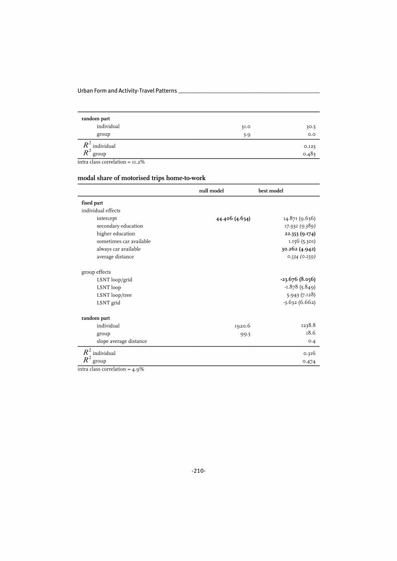
Urban Form and Activity-Travel Patterns __________________________________________
-210-
random part
individual
group
31.0
3.9
30.5
0.0
individualR2groupR2
0.125
0.483
intra class correlation = 11.2%
modal share of motorised trips home-to-work
null model best model
fixed part
individual effects
intercept
secondary education
higher education
sometimes car available
always car available
average distance
group effects
LSNT loop/grid
LSNT loop
LSNT loop/tree
LSNT grid
random part
individual
group
slope average distance
44.406 (4.634)
1920.6
99.5
14.871 (9.636)17.932 (9.389)
22.353 (9.174)
1.156 (5.301)
30.262 (4.942)0.534 (0.259)
-23.676 (8.056)
-1.878 (5.849)
5.943 (7.128)
-3.632 (6.662)
1238.8
18.6
0.4
individualR2groupR2
0.316
0.474
intra class correlation = 4.9%
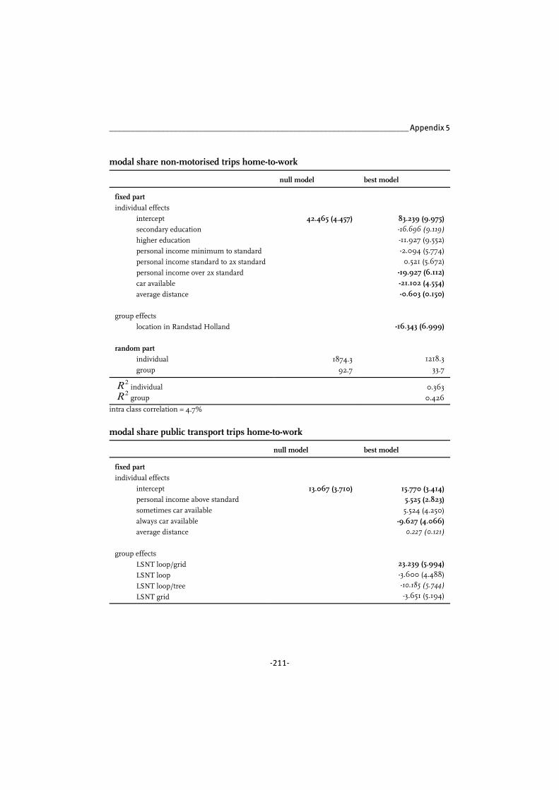
______________________________________________________________________ Appendix 5
-211-
modal share non-motorised trips home-to-work
null model best model
fixed part
individual effects
intercept
secondary education
higher education
personal income minimum to standard
personal income standard to 2x standard
personal income over 2x standard
car available
average distance
group effects
location in Randstad Holland
random part
individual
group
42.465 (4.457)
1874.3
92.7
83.239 (9.975)-16.696 (9.119)
-11.927 (9.552)
-2.094 (5.774)
0.521 (5.672)
-19.927 (6.112)-21.102 (4.554)-0.603 (0.150)
-16.343 (6.999)
1218.3
33.7
individualR2groupR2
0.363
0.426
intra class correlation = 4.7%
modal share public transport trips home-to-work
null model best model
fixed part
individual effects
intercept
personal income above standard
sometimes car available
always car available
average distance
group effects
LSNT loop/grid
LSNT loop
LSNT loop/tree
LSNT grid
13.067 (3.710) 15.770 (3.414)5.525 (2.823)
5.524 (4.250)
-9.627 (4.066)0.227 (0.121)
23.239 (5.994)
-3.600 (4.488)-10.185 (5.744)
-3.651 (5.194)

Urban Form and Activity-Travel Patterns __________________________________________
-212-
random part
individual
group
883.8
110.6
819.8
3.9
individualR2groupR2
0.172
0.498
intra class correlation = 11.1%
-213-
APPENDIX 6 | General Description Activity-Travel
Pattern Indicators
The tables listed below contain the figures that go with the general description of the
activity-travel patterns indicators reported on in section 7.3.
Cells containing significant differences at the 5% level are grey. For the ordinal
independent variables, significance of differences has been established using one-way
ANOVA or the Kruskal Wallis test, depending on whether the variances between groups
could be considered equal. For the continuous independent variables Pearson correlation
coefficient was calculated.
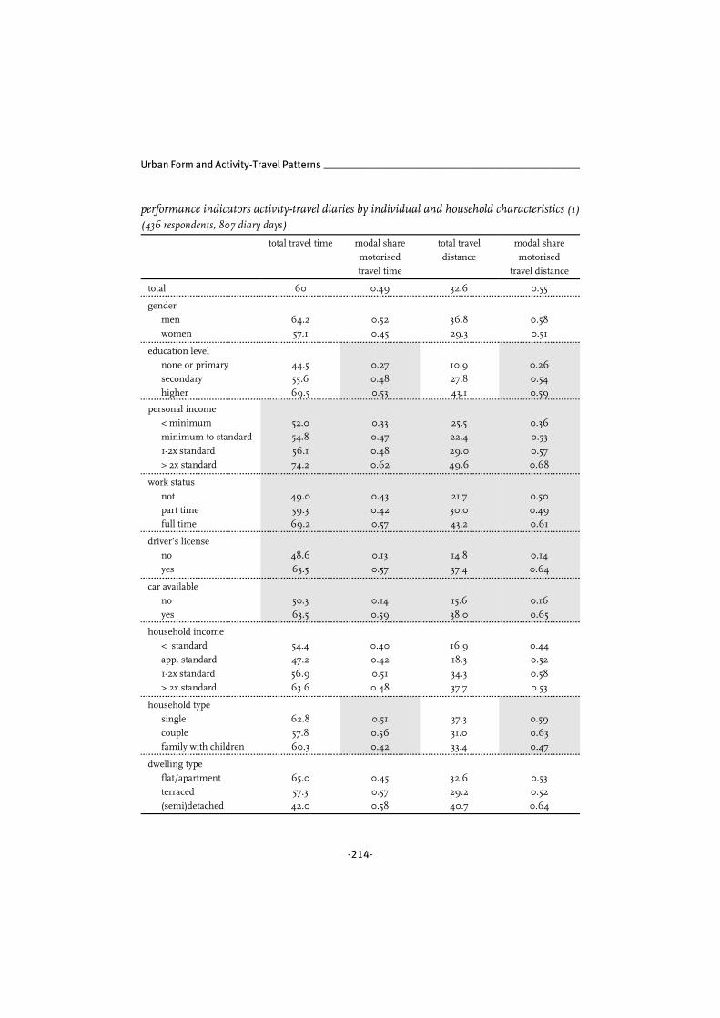
Urban Form and Activity-Travel Patterns __________________________________________
-214-
performance indicators activity-travel diaries by individual and household characteristics (1)
(436 respondents, 807 diary days)
total travel time modal share
motorised
travel time
total travel
distance
modal share
motorised
travel distance
total 60 0.49 32.6 0.55
gender
men
women
64.2
57.1
0.52
0.45
36.8
29.3
0.58
0.51
education level
none or primary
secondary
higher
44.5
55.6
69.5
0.27
0.48
0.53
10.9
27.8
43.1
0.26
0.54
0.59
personal income
< minimum
minimum to standard
1-2x standard
> 2x standard
52.0
54.8
56.1
74.2
0.33
0.47
0.48
0.62
25.5
22.4
29.0
49.6
0.36
0.53
0.57
0.68
work status
not
part time
full time
49.0
59.3
69.2
0.43
0.42
0.57
21.7
30.0
43.2
0.50
0.49
0.61
driver’s license
no
yes
48.6
63.5
0.13
0.57
14.8
37.4
0.14
0.64
car available
no
yes
50.3
63.5
0.14
0.59
15.6
38.0
0.16
0.65
household income
< standard
app. standard
1-2x standard
> 2x standard
54.4
47.2
56.9
63.6
0.40
0.42
0.51
0.48
16.9
18.3
34.3
37.7
0.44
0.52
0.58
0.53
household type
single
couple
family with children
62.8
57.8
60.3
0.51
0.56
0.42
37.3
31.0
33.4
0.59
0.63
0.47
dwelling type
flat/apartment
terraced
(semi)detached
65.0
57.3
42.0
0.45
0.57
0.58
32.6
29.2
40.7
0.53
0.52
0.64

______________________________________________________________________ Appendix 6
-215-
performance indicators activity-travel diaries by individual and household characteristics (2)
(436 respondents, 807 diary days)
trips tours trip/tour ratio
total 3.95 1.68 2.37
gender
men
women
3.59
4.21
1.55
1.77
2.36
2.39
education level
none or primary
secondary
higher
3.24
3.96
3.99
1.42
1.70
1.67
2.25
2.34
2.42
personal income
< minimum
minimum to standard
1-2x standard
> 2x standard
4.47
3.90
3.56
3.64
1.90
1.66
1.53
1.53
2.36
2.40
2.33
2.41
work status
not
part time
full time
3.89
4.57
3.78
1.68
1.98
1.59
2.29
2.31
2.44
driver’s license
no
yes
3.34
4.05
1.51
1.70
2.22
2.41
car available
no
yes
3.43
4.05
1.54
1.70
2.24
2.42
household income
< standard
app. standard
1-2x standard
> 2x standard
3.97
4.59
3.86
3.83
1.66
1.97
1.65
1.65
2.50
2.30
2.37
2.34
household type
single
couple
family with children
3.93
3.52
4.31
1.62
1.54
1.82
2.48
2.30
2.40
dwelling type
flat/apartment
terraced
(semi)detached
3.72
4.14
3.68
1.58
1.74
1.62
2.37
2.38
2.30

Urban Form and Activity-Travel Patterns __________________________________________
-216-
performance indicators activity-travel diaries by spatial characteristics (1)
(436 respondents, 807 diary days)
total travel
time
modal share
motorised travel
time
total travel
distance
modal share
motorised travel
distance
total 60 0.49 32.6 0.55
city type
concentric
lobe
poly-nuclear (Almere)
grid
62.9
56.9
64.7
57.4
0.47
0.51
0.55
0.58
37.5
31.4
38.3
25.4
0.52
0.54
0.65
0.57
transportation network type city
radial
ring
grid
50.0
64.7
61.0
0.57
0.47
0.47
23.9
36.9
33.3
0.61
0.54
0.53
transportation network type
neighbourhood
ring
loop
radial
axial
grid
tangential
56.1
63.9
60.3
57.1
68.3
67.7
0.43
0.64
0.45
0.58
0.47
0.52
30.6
37.2
38.1
26.4
32.2
35.5
0.51
0.76
0.49
0.61
0.51
0.58
local street network type
loop/grid
loop
loop/tree
grid
tree
64.3
60.6
49.8
63.4
69.7
0.52
0.49
0.57
0.38
0.53
38.0
30.0
29.1
39.9
27.9
0.62
0.52
0.66
0.44
0.59
mixed land use
no
limited
ample
60.8
59.0
62.5
0.55
0.48
0.34
33.9
30.5
40.3
0.60
0.53
0.46
shopping facilities
none or just a few
small nghbhd centre
large nghbhd centre
city district centre
city centre
72.0
58.1
52.7
54.2
62.5
0.55
0.51
0.46
0.53
0.34
36.5
32.0
28.6
24.6
40.3
0.62
0.57
0.51
0.48
0.46
location
inside Randstad
outside Randstad
66.8
55.9
0.52
0.47
32.9
32.5
0.60
0.52

______________________________________________________________________ Appendix 6
-217-
performance indicators activity-travel diaries by spatial characteristics (2)
(436 respondents, 807 diary days)
trips tours trip/tour ratio
total 3.95 1.68 2.37
city type
concentric
lobe
poly-nuclear (Almere)
grid
3.87
4.11
4.08
3.85
1.67
1.72
1.69
1.66
2.34
2.41
2.50
2.32
transportation network type city
radial
ring
grid
3.88
4.10
3.85
1.68
1.74
1.63
2.32
2.42
2.36
transportation network type
neighbourhood
ring
loop
radial
axial
grid
tangential
4.04
3.64
4.05
3.69
3.95
4.11
1.73
1.50
1.70
1.57
1.66
1.79
2.34
2.54
2.41
2.32
2.41
2.36
local street network type
loop/grid
loop
loop/tree
grid
tree
3.94
4.10
3.36
4.30
4.11
1.65
1.77
1.45
1.78
1.76
2.46
2.34
2.31
2.46
2.33
mixed land use
no
limited
ample
3.94
4.02
3.61
1.67
1.71
1.55
2.37
2.38
2.35
shopping facilities
none or just a few
small nghbhd centre
large nghbhd centre
city district centre
city centre
4.20
3.99
3.80
3.87
3.61
1.76
1.71
1.63
1.58
1.55
2.47
2.35
2.30
2.49
2.35
location
inside Randstad
outside Randstad
4.04
3.90
1.69
1.67
2.43
2.34

Urban Form and Activity-Travel Patterns __________________________________________
-218-
correlation coefficients performance indicators activity-travel diaries (1)(436 respondents, 807 diary days)
total travel
time
modal share
motorised
travel time
total travel
distance
modal share
motorised
travel distance
age -0.03 0.11 -0.05 0.17
distance to city centre -0.02 -0.09 -0.06 0.08
distance to ic station -0.06 -0.07 -0.08 0.07
employment 0.09 -0.06 -0.06 -0.08
population density nghbhd 0 -0.04 -0.01 -0.03
housing density nghbhd -0.01 -0.05 -0.03 -0.04
population density city 0.07 0.03 -0.05 0.03
housing density city 0.07 0.03 -0.05 0.03
degree urbanisation nghbhd -0.12 0.09 -0.05 0.11
degree urbanisation city 0 -0.04 0.09 -0.05
correlation coefficients performance indicator activity-travel diaries (2)(436 respondents, 807 diary days)
trips tours trip/tour ratio
age -0.06 -0.02 -0.12
distance to city centre 0 0.02 -0.02
distance to ic station -0.02 0 -0.03
employment -0..01 0 -0.07
population density nghbhd 0.05 0.06 0.01
housing density nghbhd 0.03 0.04 0.01
population density city 0.04 0.03 0.04
housing density city 0.04 0.03 0.03
degree urbanisation nghbhd -0.09 -0.06 -0.06
degree urbanisation city -0.02 -0.02 0.01

______________________________________________________________________ Appendix 6
-219-
performance indicators activity-travel diaries weekdays by individual and householdcharacteristics (1) (320 respondents, 528 diary days)
total travel
time
modal share
motorised traveltime
total travel
distance
modal share
motorised traveldistance
total 69.6 0.48 37.4 0.55
gender
menwomen
77.065.6
0.510.45
46.630.4
0.560.52
education levelnone or primary
secondaryhigher
57.2
64.781.3
0.17
0.480.53
11.3
31.650.6
0.17
0.550.60
personal income< minimum
minimum to standard1-2x standard
> 2x standard
67.0
65.661.6
85.3
0.31
0.490.47
0.60
29.1
26.729.7
61.1
0.36
0.540.55
0.67
work status
notpart time
full time
58.065.6
80.8
0.410.41
0.57
24.152.3
27.7
0.510.61
0.48
driver’s license
noyes
63.672.7
0.150.55
15.243.2
0.150.62
car availableno
yes
64.9
72.8
0.16
0.57
16.6
44.1
0.17
0.64
household income
< standardapp. standard
1-2x standard> 2x standard
68.751.4
69.673.1
0.690.31
0.540.48
23.020.6
44.441.8
0.390.41
0.570.55
household typesingle
couplefamily with children
73.6
66.069.0
0.51
0.560.41
46.5
38.733.1
0.55
0.630.48
dwelling typeflat/apartment
terraced(semi)detached
80.8
64.074.7
0.49
0.430.59
40.7
31.350.4
0.54
0.510.63
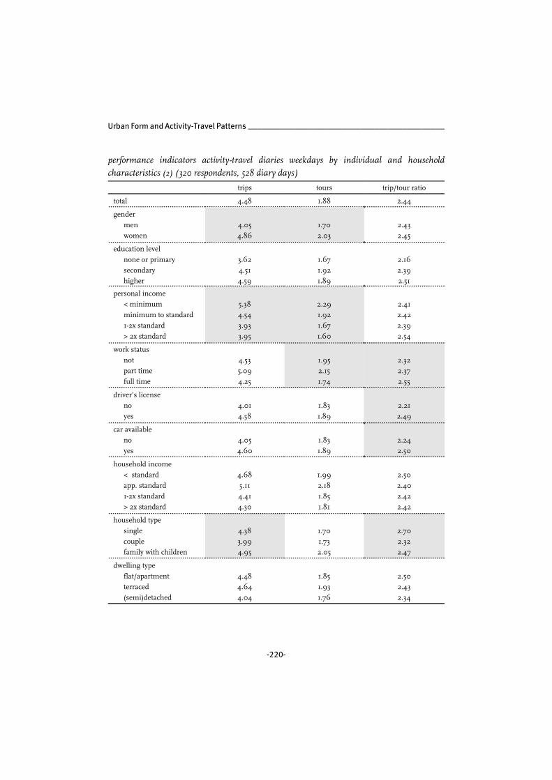
Urban Form and Activity-Travel Patterns __________________________________________
-220-
performance indicators activity-travel diaries weekdays by individual and householdcharacteristics (2) (320 respondents, 528 diary days)
trips tours trip/tour ratio
total 4.48 1.88 2.44
gender
men
women
4.05
4.86
1.70
2.03
2.43
2.45
education level
none or primary
secondary
higher
3.62
4.51
4.59
1.67
1.92
1.89
2.16
2.39
2.51
personal income
< minimum
minimum to standard
1-2x standard
> 2x standard
5.38
4.54
3.93
3.95
2.29
1.92
1.67
1.60
2.41
2.42
2.39
2.54
work status
not
part time
full time
4.53
5.09
4.25
1.95
2.15
1.74
2.32
2.37
2.55
driver’s license
no
yes
4.01
4.58
1.83
1.89
2.21
2.49
car available
no
yes
4.05
4.60
1.83
1.89
2.24
2.50
household income
< standard
app. standard
1-2x standard
> 2x standard
4.68
5.11
4.41
4.30
1.99
2.18
1.85
1.81
2.50
2.40
2.42
2.42
household type
single
couple
family with children
4.38
3.99
4.95
1.70
1.73
2.05
2.70
2.32
2.47
dwelling type
flat/apartment
terraced
(semi)detached
4.48
4.64
4.04
1.85
1.93
1.76
2.50
2.43
2.34

______________________________________________________________________ Appendix 6
-221-
performance indicators activity-travel diaries weekdays by spatial characteristics (1)
(320 respondents, 528 diary days)
total travel
time
modal share
motorised traveltime
total travel
distance
modal share
motorised traveldistance
total 69.6 0.48 37.4 0.55
city type
concentriclobe
poly-nuclear (Almere)grid
71.262.1
79.470.5
0.460.47
0.530.49
38.834.6
48.533.5
0.500.51
0.660.58
transportation network type cityradial
ringgrid
52.8
77.971.4
0.51
0.470.48
23.0
46.536.9
0.56
0.540.54
transportation network typeneighbourhood
ringloop
radialaxial
gridtangential
66.074.3
68.859.8
88.285.6
0.450.58
0.460.55
0.410.47
33.144.0
47.426.1
41.245.8
0.540.71
0.480.59
0.460.54
local street network typeloop/grid
looploop/tree
gridtree
83.1
65.851.3
82.575.7
0.54
0.420.59
0.420.55
51.5
27.128.8
57.634.3
0.66
0.470.68
0.460.61
mixed land useno
limitedample
69.8
66.290.9
0.54
0.440.47
41.8
30.663.6
0.59
0.510.57
shopping facilitiesnone or just a few
small nghbhd centrelarge nghbhd centre
city district centrecity centre
82.9
66.358.5
54.390.9
0.47
0.500.46
0.410.47
40.3
38.625.4
19.863.6
0.57
0.560.52
0.400.57
locationinside Randstad
outside Randstad
80.2
62.8
0.51
0.46
41.0
35.1
0.61
0.51

Urban Form and Activity-Travel Patterns __________________________________________
-222-
performance indicators activity-travel diaries weekdays by spatial characteristics (2)
(320 respondents, 528 diary days)
trips tours trip/tour ratio
total 4.48 1.88 2.44
city type
concentric
lobe
poly-nuclear (Almere)
grid
4.53
4.47
4.44
4.46
1.92
1.87
1.78
1.87
2.45
2.41
2.60
2.38
transportation network type city
radial
ring
grid
4.33
4.63
4.53
1.87
1.90
1.85
2.32
2.53
2.43
transportation network type
neighbourhood
ring
loop
radial
axial
grid
tangential
4.51
4.02
4.52
4.00
4.97
5.18
1.88
1.59
1.90
1.71
2.03
2.19
2.44
2.62
2.45
2.31
2.55
2.47
local street network type
loop/grid
loop
loop/tree
grid
tree
4.39
4.64
3.70
5.00
4.56
1.78
1.96
1.59
2.06
1.93
2.60
2.42
2.32
2.51
2.35
mixed land use
no
limited
ample
4.38
4.52
4.65
1.85
1.88
1.91
2.39
2.45
2.60
shopping facilities
none or just a few
small nghbhd centre
large nghbhd centre
city district centre
city centre
4.79
4.53
4.12
4.00
4.65
1.92
1.93
1.73
1.67
1.91
2.59
2.36
2.39
2.49
2.60
location
inside Randstad
outside Randstad
4.66
4.37
1.90
1.86
2.53
2.38

______________________________________________________________________ Appendix 6
-223-
correlation coefficients performance indicators activity-travel diaries weekdays(1)(320 respondents, 528 diary days)
total travel
time
modal share
motorised
travel time
total travel
distance
modal share
motorised
travel distance
age -0.12 0.08 -0.1 0.18
distance to city centre -0.11 0 -0.15 -0.01
distance to ic station -0.13 0.04 -0.13 0.04
employment -0.13 -0.05 -0.08 -0.09
population density nghbhd 0.07 -0.06 0.03 -0.03
housing density nghbhd 0.1 -0.05 0.05 -0.02
population density city 0.1 0.03 0 0.04
housing density city 0.1 0.03 -0.01 0.03
degree urbanisation nghbhd -0.21 0.06 -0.12 0.08
degree urbanisation city -0.02 -0.03 0.05 -0.03
correlation coefficients performance indicators activity-travel diaries weekdays(2)(320 respondents, 528 diary days)
trips tours trip/tour ratio
age -0.07 -0.05 -0.09
distance to city centre -0.02 0 -0.05
distance to ic station -0.07 -0.04 -0.07
employment -0.03 -0.01 -0.1
population density nghbhd 0.1 0.1 0.03
housing density nghbhd 0.08 0.08 0.02
population density city 0.07 0.06 0.02
housing density city 0.07 0.06 0.01
degree urbanisation nghbhd -0.12 -0.09 -0.08
degree urbanisation city -0..05 -0.05 0.04

-224-
APPENDIX 7 | Multilevel Analyses Activity Diaries
The tables listed below report the results from the multilevel analyses on activity diary
indicators, as discussed in chapter 7. The analyses reported in this appendix are based
on data on 467 diary days, 320 of which concern weekdays.
Parameters reported in bold face type are significant at the 5% level, parameters reported
in italics are significant at the 10% level. The tables report parameter values and t-values,
as is usual when reporting multilevel analysis results.
In the tables the following abbreviations are used for layout reasons:
TNTC = transportation network type city
TNTN = transportation network type neighbourhood
LSNT = local street network type

______________________________________________________________________ Appendix 7
-225-
total travel time
null model best model
fixed part
individual effect
intercept
personal income (minimum to standard)
personal income (standard to 2x standard)
personal income (over 2x standard)
group effects
TNTC radial
TNTC ring
interaction effects
> 2x standard*TNTC radial
> 2x standard*TNTC ring
random part
individual
group
slope > 2x standard
64.523 (3.251)
2289.28
45.75
63.033 (3.574)
-3.075 (4.880)
-3.069 (4.733)
15.633 (5.489)
-8.860 (5.446)9.252 (4.807)
-7.584 (7.327)
13.679 (6.384)
2120.23
80.58
114.97
individualR2groupR2
0.050
0.000
intra class correlation = 1.9%
total motorised transport travel time
null model best model
fixed part
individual effect
intercept
personal income (minimum to standard)
personal income (standard to 2x standard)
personal income (over 2x standard)
sometimes car available
always car available
interaction effects
> 2x standard*limited land use mix
> 2x standard*ample land use mix
34.497 (2.534) 29.389 (2.539)
-2.247 (4.118)
-5.225 (4.058)
24.803 (5.038)
4.931 (3.513)
12.490 (3.197)
-15.933 (6.244)29.712 (9.375)
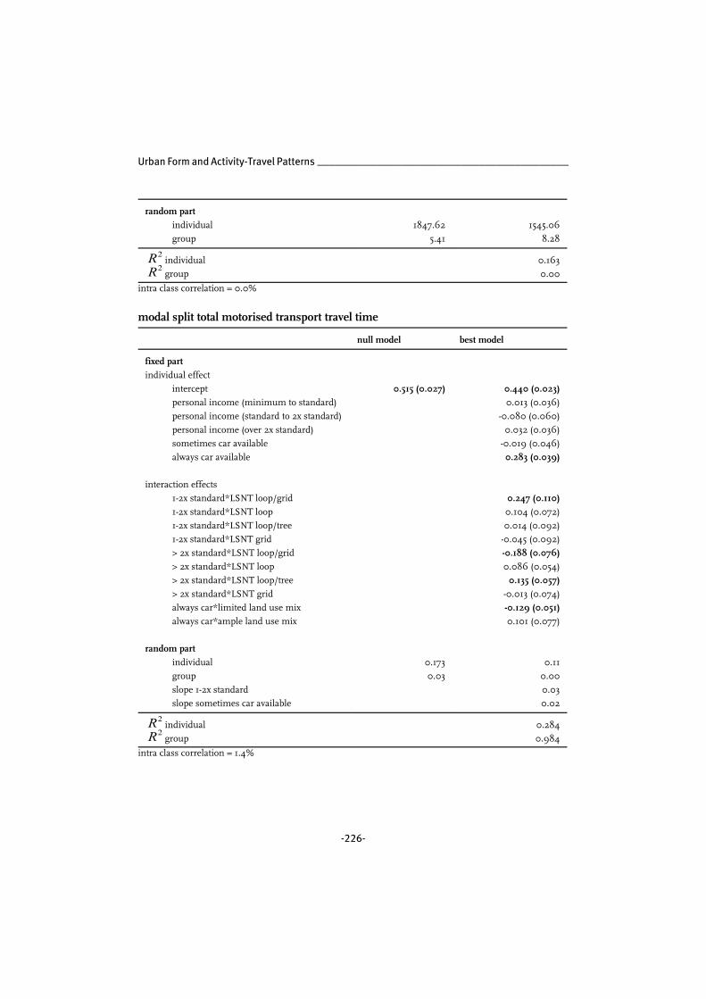
Urban Form and Activity-Travel Patterns __________________________________________
-226-
random part
individual
group
1847.62
5.41
1545.06
8.28
individualR2groupR2
0.163
0.00
intra class correlation = 0.0%
modal split total motorised transport travel time
null model best model
fixed part
individual effect
intercept
personal income (minimum to standard)
personal income (standard to 2x standard)
personal income (over 2x standard)
sometimes car available
always car available
interaction effects
1-2x standard*LSNT loop/grid
1-2x standard*LSNT loop
1-2x standard*LSNT loop/tree
1-2x standard*LSNT grid
> 2x standard*LSNT loop/grid
> 2x standard*LSNT loop
> 2x standard*LSNT loop/tree
> 2x standard*LSNT grid
always car*limited land use mix
always car*ample land use mix
random part
individual
group
slope 1-2x standard
slope sometimes car available
0.515 (0.027)
0.173
0.03
0.440 (0.023)
0.013 (0.036)
-0.080 (0.060)
0.032 (0.036)
-0.019 (0.046)
0.283 (0.039)
0.247 (0.110)
0.104 (0.072)
0.014 (0.092)
-0.045 (0.092)
-0.188 (0.076)
0.086 (0.054)
0.135 (0.057)
-0.013 (0.074)
-0.129 (0.051)
0.101 (0.077)
0.11
0.00
0.03
0.02
individualR2groupR2
0.284
0.984
intra class correlation = 1.4%

______________________________________________________________________ Appendix 7
-227-
total number of tours
null model best model
fixed part
individual effect
intercept
household income (app. standard)
household income (standard to 2x standard)
household income (over 2x standard)
working full time
working part time
random part
individual
group
1.695 (0.052)
0.83
0.00
1.857 (0.071)0.321 (0.148)
-0.110 (0.107)
-0.133 (0.083)
0.264 (0.091)-0.203 (0.071)
0.79
0.00
individualR2groupR2
0.039
0.471
intra class correlation = 0.0%
total number of trips
null model best model
fixed part
individual effect
intercept
household income (app. standard)
household income (standard to 2x standard)
household income (over 2x standard)
car available
couple
family with children
working part time
working full time
group effects
LSNT loop/grid
LSNT loop
LSNT loop/tree
LSNT grid
4.000 (0.129) 3.984 (0.217)0.939 (0.369)
-0.296 (0.279)
-0.198 (0.221)
0.633 (0.160)-0.620 (0.216)0.456 (0.205)
0.106 (0.268)
-0.567 (0.176)
-0.362 (0.330)
-0.355 (0.244)
0.047 (0.307)
0.649 (0.295)

Urban Form and Activity-Travel Patterns __________________________________________
-228-
interaction effects
1-2x standard*TNTN ring
1-2x standard*TNTN loop
1-2x standard*TNTN radial
1-2x standard*TNTN axial
1-2x standard*TNTN grid
couple*LSNT loop/grid
couple*LSNT loop
couple*LSNT loop/tree
couple*LSNT grid
part time*TNTN ring
part time*TNTN loop
part time*TNTN radial
part time*TNTN axial
part time*TNTN grid
random part
individual
group
5.02
0.00
-0.480 (0.420)1.002 (0.577)
-0.924 (0.464)
0.619 (0.527)
-0.686 (0.762)
-0.145 (0.482)
1.086 (0.345)
-0.351 (0.352)
-0.267 (0.359)
0.431 (0.348)
-0.706 (0.621)
0.503 (0.402)
1.016 (0.379)
-1.142 (0.756)
4.36
0.00
individualR2groupR2
0.131
0.893
intra class correlation = 0.0%
ratio total number of tours / trips
null model best model
fixed part
individual effect
intercept
higher education
car available
couple
family with children
random part
individual
group
2.381 (0.042)
0.31
0.01
2.358 (0.048)0.059 (0.033)
0.095 (0.040)-0.125 (0.047)
0.022 (0.047)
0.30
0.01
individualR2groupR2
0.034
0.280
intra class correlation = 3.6%

______________________________________________________________________ Appendix 7
-229-
total travel distance
null model best model
fixed part
individual effect
intercept
personal income (minimum to standard)
personal income (standard to 2x standard)
personal income (over 2x standard)
car available
working part time
working full time
group effects
degree of urbanisation city
random part
individual
group
36.604 (3.210)
2893.72
12.08
27.221 (4.079)
-7.977 (5.494)
-6.661 (5.426)
12.246 (5.201)9.833 (3.912)
-0.141 (5.439)8.567 (4.524)
-8.765 (4.578)
2674.29
6.97
individualR2groupR2
0.076
0.423
intra class correlation = 0.4%
total travel distance motorised transport
null model best model
fixed part
individual effect
intercept
personal income (minimum to standard)
personal income (standard to 2x standard)
personal income (over 2x standard)
car available
multi-person household
group effects
distance to inter-city station
interaction effects
> 2x standard*distance to city centre
22.272 (2.398) 19.652 (3.335)-8.880 (3.961)
-3.404 (3.912)
18.252 (3.661)10.282 (2.880)-6.071 (3.090)
-3.217 (1.387)
-8.057 (2.273)

Urban Form and Activity-Travel Patterns __________________________________________
-230-
random part
individual
group
1719.79
1.83
1430.86
1.00
individualR2groupR2
0.168
0.454
intra class correlation = 0.0%
modal split total distance motorised transport
null model best model
fixed part
individual effect
intercept
sometimes car available
always car available
group effects
LSNT loop/grid
LSNT loop
LSNT loop/tree
LSNT grid
interaction effects
always car available*land use mix
random part
individual
group
0.548 (0.031)
0.19
0.01
0.443 (0.026)
-0.006 (0.032)
0.303 (0.029)
0.002 (0.051)
0.008 (0.036)
0.097 (0.043)
-0.063 (0.046)
-0.050 (0.026)
0.13
0.00
individualR2groupR2
0.275
0.988
intra class correlation = 3.0%
travel time on weekdays
null model best model
fixed part
individual effect
intercept
higher education
children in household
90.088 (9.182) 97.713 (8.992)
13.644 (10.195)
-24.198 (8.124)
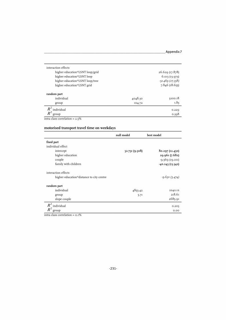
______________________________________________________________________ Appendix 7
-231-
interaction effects
higher education*LSNT loop/grid
higher education*LSNT loop
higher education*LSNT loop/tree
higher education*LSNT grid
random part
individual
group
4048.30
104.72
26.629 (17.878)
6.013 (13.973)-52.469 (27.358)
7.846 (18.655)
3200.18
1.83
individualR2groupR2
0.229
0.398
intra class correlation = 2.5%
motorised transport travel time on weekdays
null model best model
fixed part
individual effect
intercept
higher education
couple
family with children
interaction effects
higher education*distance to city centre
random part
individual
group
slope couple
52.731 (9.508)
4853.42
5.71
80.297 (12.450)29.961 (7.682)
-9.569 (19.101)
-40.243 (13.342)
-9.650 (5.474)
2242.12
218.61
2685.91
individualR2groupR2
0.203
0.00
intra class correlation = 0.1%

Urban Form and Activity-Travel Patterns __________________________________________
-232-
modal split motorised transport travel time on weekdays
null model best model
fixed part
individual effect
intercept
higher education
sometimes car available
always car available
group effects
population density neighbourhood
random part
individual
group
0.546 (0.059)
0.19
0.00
0.572 (0.062)0.132 (0.056)
0.038 (0.078)
0.178 (0.068)
0.005 (0.003)
0.12
0.00
individualR2groupR2
0.337
0.230
intra class correlation = 0.1%
number of tours on weekdays
null model best model
fixed part
individual effect
intercept
personal income (minimum to standard)
personal income (standard to 2x standard)
personal income (over 2x standard)
random part
individual
group
slope personal income (over 2x standard)
2.000 (0.152)
1.25
0.00
2.024 (0.138)
-0.008 (0.234)
-0.561 (0.204)
-0.298 (0.292)
0.81
0.03
0.43
individualR2groupR2
0.171
0.170
intra class correlation = 0.0%

______________________________________________________________________ Appendix 7
-233-
number of trips on weekdays
null model best model
fixed part
individual effect
intercept
personal income standard and over
sometimes car available
always car available
group effects
limited land use mix
ample land use mix
random part
individual
group
4.760 (0.384)
7.92
0.01
5.631 (0.584)-1.005(0.391)1.188 (0.563)
-0.100 (0.535)
-1.389 (0.712)
1.574 (1.064)
6.54
0.00
individualR2groupR2
0.175
0.181
intra class correlation = 0.1%
ratio number of tours / trips on weekdays
null model best model
fixed part
individual effect
intercept
higher education
terraced house
(semi)detached house
group effects
limited land use mix
ample land use mix
interaction effects
higher education* limited mixing
higher education* ample mixing
random part
individual
group
2.444 (0.107)
0.61
0.00
2.804 (1.334)0.600 (0.129)
0.234 (0.120)
-0.191 (0.140)
-0.571 (0.180)0.843 (0.275)
-0.451 (0.169)0.587 (0.249)
0.37
0.00

Urban Form and Activity-Travel Patterns __________________________________________
-234-
individualR2groupR2
0.394
0.395
intra class correlation = 0.1%
travel distance on weekdays
null model best model
fixed part
individual effect
intercept
personal income minimum to standard
personal income standard to 2x standard
personal income over 2x standard
couple
family with children
interaction effects
income min-standard*distance city centre
income min-standard*LSNT loop/grid
income min-standard*LSNT loop
income min-standard*LSNT loop/tree
income min-standard*LSNT grid
income 1-2x standard*LSNT loop/grid
income 1-2x standard*LSNT loop
income 1-2x standard*LSNT loop/tree
income 1-2x standard*LSNT grid
couple*LSNT loop/grid
couple*LSNT loop
couple*LSNT loop/tree
couple*LSNT grid
random part
individual
group
slope family with children
55.925 (10.747)
6201.02
7.11
131.053 (20.150)
2.131 (24.169)
-108.411 (36.327)35.156 (15.591)
-32.907 (23.195)
-102.555 (26.115)
-21.458 (9.994)-167.616 (68.629)
11.80 (29.028)
157.871 (60.610)
52.117 (47.319)
136.879 (47.272)68.887 (36.468)
-43.404 (83.644)
-42.162 (45.879)
-95.005 (31.729)-54.987 (27.136)
-113.302 (45.698)232.003 (45.838)
2180.14
503.26
4781.97
individualR2groupR2
0.144
0.145
intra class correlation = 0.1%

______________________________________________________________________ Appendix 7
-235-
travel distance motorised transport on weekdays
null model best model
fixed part
individual effect
intercept
higher education
couple
family with children
group effects
LSNT loop/grid
LSNT loop
LSNT loop/tree
LSNT grid
interaction effects
higher education*LSNT loop/grid
higher education*LSNT loop
higher education*LSNT loop/tree
higher education*LSNT grid
couple*LSNT loop/grid
couple*LSNT loop
couple*LSNT loop/tree
couple*LSNT grid
random part
individual
group
38.704 (9.861)
5221.64
5.72
81.905 (17.341)20.685 (12.143)
-22.748 (20.903)
-73.282 (17.265)
57.741 (22.625)
18.209 (20.964)
-6.623 (52.382)
-21.713 (23.961)
-16.650 (20.414)
-1.178 (15.738)
-18.685 (30.965)
53.947 (19.815)-67.287 (29.694)
-38.854 (29.498)
-50.534 (61.898)
72.346 (34.057)
2704.63
1.12
individualR2groupR2
0.482
0.486
intra class correlation = 0.1%
modal split distance motorised transport on weekdays
null model best model
fixed part
individual effect
intercept
higher education
car available
0.562 (0.061) 0.533 (0.070)0.121 (0.057)
0.201 (0.063)
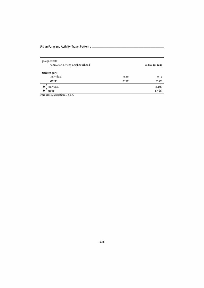
Urban Form and Activity-Travel Patterns __________________________________________
-236-
group effects
population density neighbourhood
random part
individual
group
0.20
0.00
0.006 (0.003)
0.13
0.00
individualR2groupR2
0.356
0.366
intra class correlation = 0.2%

-237-
AUTHOR INDEX
Abraham 132, 137
Arentze 65, 68, 111, 114, 134, 140
AVV 6, 134
Axhausen 44, 111, 134
Banister 31, 134, 143
Boarnet 27, 134
Bolt 56, 134
Borgers 65, 140
Bosker 90, 91, 92, 140
Brown 40, 136, 144
Brög 51, 137
Bryk 90, 93, 116, 134
Bullen 93, 134
CBS (Statistics Netherlands) 6, 7, 8,
84, 135
Cervero 34, 35, 38, 47, 77, 135, 144
Chapin 44, 135
Clarke 51, 135
Congress for the New Urbanism (CNU)
22, 77, 135
Coombes 93, 135
Congdon 93, 116, 134
Crane 24, 26, 135
Dix 51, 135
Duncan 93, 134
Dijst 51, 135
Dumbaugh 40, 136, 144
Ettema 3, 50, 52, 63, 136
Ewing 32, 40, 136, 144, 145
Florez 34, 77, 136, 145
Frank 30, 136, 143
Friedman 32, 77, 136, 145
Gärling 44, 134
Gibson 24, 136
Giuliano 25, 136
Golob 51, 136
Gordon, I. 28, 136, 142
Gordon, S.P. 32, 77, 136, 145
Gorham 36, 135, 144
Haliyur 32, 136, 145
Hägerstrand 44, 136
Handy 28, 29, 33, 136, 142, 145
Hanson 27, 35, 47, 136, 145
Heidemij Advies 17, 138
Hilbers 24, 25, 140
Hofman 111, 134
Hox 90, 93, 136
HSPE-council 2, 5, 8, 15, 17, 136
Hunt 132, 137
Ibrahim 29, 137, 142

Urban Form and Activity-Travel Patterns __________________________________________
-238-
Janse 19, 137
Jones, K. 93, 134
Jones, P. 51, 135
Kalfs 111, 134
Kasturi 27, 38, 93, 140, 147
Kenworthy 28, 29, 139, 142
Kitamura 3, 27, 37, 46, 47, 93, 137,
145
Klerk, de 55, 137
Kockelman 38, 47, 77, 135, 144
Konings 37, 137, 146
Kruythoff 37, 137, 146
Laidet 3, 27, 37, 46, 47, 93, 137, 145
Larsen 36, 139, 146
Maat 37, 137, 146
McCormack 33, 137, 139, 146, 147
McMillan 132, 137
McNally 25, 137
Miller 29, 137, 142
Meurs 51, 136
Meyburg 51, 137
Ministry of EA (EZ) 10, 19, 138, 139
Ministry of HSP( VRO) 8, 9, 137
Ministry of HSPE (VROM) 9, 10, 11,
12, 15, 16, 137, 138
Ministry of TPWWM (V&W) 10, 11,
12, 13, 15, 17, 138
Mogridge 19, 138, 142
Mokhtarian 3, 27, 37, 46, 47, 93, 137,
145
MuConsult 27, 39, 138, 146
Murakami 51, 139
Nasar 34, 77, 139, 146
Newman 28, 29, 139, 142
Niemi 51, 139
NOVEM 19, 137, 139
Næss 26, 27, 29, 30, 31, 36, 47, 139,
142, 143, 146
Page 32, 136, 145
Peers 32, 77, 136, 145
Pivo 30, 136, 143
Raudenbush 90, 93, 116, 134
Raybould 93, 135
Rottier 55, 139
Ryan 25, 137
Røe 27, 31, 36, 39, 139, 143, 146
Sarmiento 27, 134
Sandberg 27, 30, 31, 139, 142, 143
Schimek 28, 29, 139, 142
Scott Rutherford 33, 137, 139, 146, 147
Small 25, 136
Smits 24, 25, 140
Snellen 65, 140
Snijders 90, 91, 92, 140
Stopher 51, 140
Sun 27, 38, 93, 140, 147
Timmermans 3, 44, 50, 52, 63, 65,
68, 111, 114, 134, 136, 140
Verroen 14, 24, 25, 140
Watson 31, 134, 143
Watterson 51, 139
WCED 10, 12, 140

_______________________________________________________________________ Author Index
-239-
Wilkinson 33, 137, 139, 146, 147
Wilmot 27, 38, 93, 140, 147
Wood 31, 134, 143
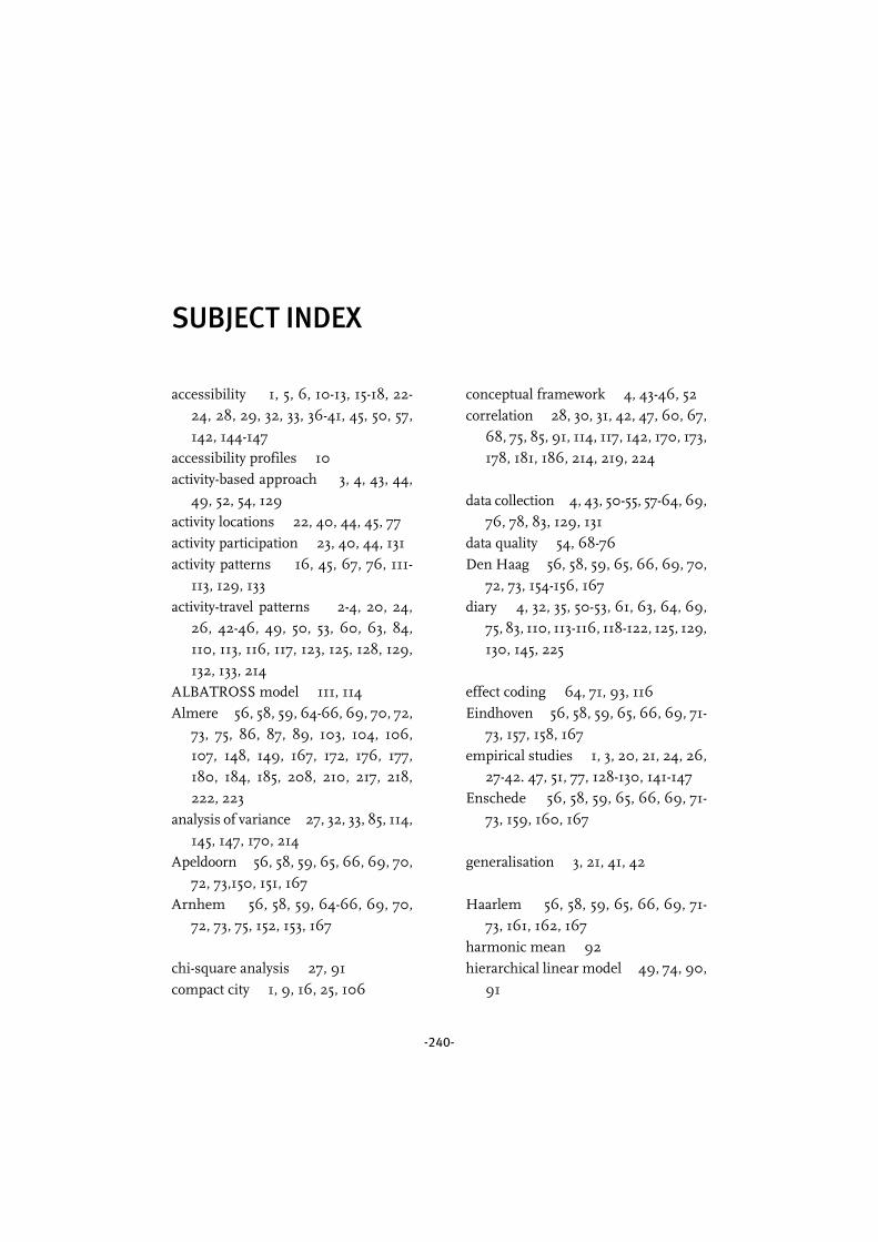
-240-
SUBJECT INDEX
accessibility 1, 5, 6, 10-13, 15-18, 22-
24, 28, 29, 32, 33, 36-41, 45, 50, 57,
142, 144-147
accessibility profiles 10
activity-based approach 3, 4, 43, 44,
49, 52, 54, 129
activity locations 22, 40, 44, 45, 77
activity participation 23, 40, 44, 131
activity patterns 16, 45, 67, 76, 111-
113, 129, 133
activity-travel patterns 2-4, 20, 24,
26, 42-46, 49, 50, 53, 60, 63, 84,
110, 113, 116, 117, 123, 125, 128, 129,
132, 133, 214
ALBATROSS model 111, 114
Almere 56, 58, 59, 64-66, 69, 70, 72,
73, 75, 86, 87, 89, 103, 104, 106,
107, 148, 149, 167, 172, 176, 177,
180, 184, 185, 208, 210, 217, 218,
222, 223
analysis of variance 27, 32, 33, 85, 114,
145, 147, 170, 214
Apeldoorn 56, 58, 59, 65, 66, 69, 70,
72, 73,150, 151, 167
Arnhem 56, 58, 59, 64-66, 69, 70,
72, 73, 75, 152, 153, 167
chi-square analysis 27, 91
compact city 1, 9, 16, 25, 106
conceptual framework 4, 43-46, 52
correlation 28, 30, 31, 42, 47, 60, 67,
68, 75, 85, 91, 114, 117, 142, 170, 173,
178, 181, 186, 214, 219, 224
data collection 4, 43, 50-55, 57-64, 69,
76, 78, 83, 129, 131
data quality 54, 68-76
Den Haag 56, 58, 59, 65, 66, 69, 70,
72, 73, 154-156, 167
diary 4, 32, 35, 50-53, 61, 63, 64, 69,
75, 83, 110, 113-116, 118-122, 125, 129,
130, 145, 225
effect coding 64, 71, 93, 116
Eindhoven 56, 58, 59, 65, 66, 69, 71-
73, 157, 158, 167
empirical studies 1, 3, 20, 21, 24, 26,
27-42. 47, 51, 77, 128-130, 141-147
Enschede 56, 58, 59, 65, 66, 69, 71-
73, 159, 160, 167
generalisation 3, 21, 41, 42
Haarlem 56, 58, 59, 65, 66, 69, 71-
73, 161, 162, 167
harmonic mean 92
hierarchical linear model 49, 74, 90,
91

______________________________________________________________________ Subject Index
-241-
Kruskal-Wallis test 85, 114, 170, 214
Leeuwarden 56, 58, 59, 65, 66, 69,
71-73, 163, 164, 167
location policy 1, 9-11, 13, 15-20
matched pair analysis 32, 34, 36, 144
methodological flaws 3, 42, 43, 52
mobility 1-3, 5-10, 12, 13, 15-17, 20, 23-
25, 38, 41-43, 46, 50, 52, 90, 93, 106,
124, 128, 130, 132, 142
mobility profiles 10, 11
mobility reduction 1-3, 8, 10, 16, 17,
20, 22, 24, 28, 41, 42, 76, 129, 132,
133
modal shift 8, 15-17, 20, 31
modal split 26, 29, 30, 34, 37, 86, 93,
95-98, 100, 101, 103, 105, 114, 115,
117, 120-122, 124, 125, 132, 170
model performance 94-97, 117-118
morphology 3, 55, 56
multilevel analysis 74, 75, 84, 90, 91,
93, 94, 97, 105, 110, 116, 118, 122,
123, 129, 187-213, 225-237
multilevel model 84, 90-93, 116-118
neo-traditional design 24-26, 32-35,
77
New Urbanism 22, 24, 38, 77, 124
probit regression analysis 64-66
Poisson regression 93
quasi-experimental design 43, 46, 47,
52, 54, 129, 131
questionnaire 4, 50-52, 54, 61-64, 67,
68, 82, 83, 113
regression analysis 29-31, 34-40, 42,
46, 47, 71-75, 91, 93, 142-147, 169
research design 4, 42, 53, 54, 129, 131
response 4, 51, 54, 64-66, 75, 83, 85,
93, 113, 116, 131, 167
sample 21, 47, 49, 66-68, 77, 106,
129, 132
simulation studies 21, 24-26, 41, 91
socioeconomic characteristics
definitions 82, 168-169
spatial characteristics
definitions 78-82
spatial mobility policy 1-3, 5-21, 25,
42, 50, 76, 77, 129-132
spatial planning 1, 2, 4-6, 8, 10, 11, 15-
17, 19, 29, 41, 50, 56, 128, 132
standardised coefficients 98-104, 118-
120, 122
sustainability 1, 12, 43, 45, 133
theoretical studies 21-24, 28, 40, 41,
77, 124, 130
transportation models 25, 26
travel behaviour 21-41, 43, 50, 63, 84-
130, 132
travel patterns 2, 3, 22, 24, 25, 27, 28,
32, 33, 45, 46, 52, 67, 76, 82, 88, 123,
124, 129, 130, 133
travel survey 27, 28, 32, 36, 38, 39, 51,
66, 68, 110, 142, 143, 145, 147

Urban Form and Activity-Travel Patterns __________________________________________
-242-
urban design 1, 2, 9, 12, 16-19, 22-26,
32, 36, 38, 40, 41, 43, 46, 50, 52, 56,
76, 77, 130-133
urban form 1-4, 14, 16, 17, 20-22, 24,
26-28, 31, 40-43, 45, 46, 52, 54-61,
75-824, 98, 100, 102, 103, 105-110,
119-132
validity 21, 26, 52
VINEX 1, 10, 15
Zoetermeer 56, 58, 59, 65, 66, 69,
71-73, 165-167

-243-
SAMENVATTING (DUTCH SUMMARY)
In Nederland wordt de laatste jaren hard gewerkt aan de ontwikkeling van VINEX-
wijken. Deze grote woningbouwlocaties zijn het resultaat van het Rijksbeleid in de jaren
negentig en moeten ervoor zorgen dat aan de enorme woningvraag voldaan wordt. Bij
het ontwerp van deze locaties worden belangrijke beslissingen genomen met betrekking
tot de ruimtelijke structuur van de wijken. De inrichting zou moeten bijdragen aan het
realiseren van beleidsdoelen zoals duurzaamheid en vermindering van de
automobiliteit. Het is echter onduidelijk welke ruimtelijke inrichting de beste bijdrage
levert aan deze doelen. Empirische kennis op dit punt ontbreekt grotendeels. In de
literatuur zien we veelvuldig dat ruimtelijke inrichting in verband wordt gebracht met
mobiliteit. Maar helaas zijn er een aantal bezwaren in te brengen tegen deze literatuur.
Meestal wordt gerapporteerd over studies die uitgevoerd zijn in andere landen en op
andere continenten, hetgeen vragen oproept over de toepasbaarheid in de Nederlandse
situatie. Daarnaast kennen bestaande studies een aantal methodologische bezwaren.
De studie die in dit proefschrift wordt gerapporteerd is erop gericht de relatie tussen
ruimtelijke inrichting en de reductie van (auto)mobiliteit empirisch te testen in de
Nederlandse situatie. De vraag daarbij is of er een relatie is tussen ruimtelijke inrichting
en verplaatsingspatronen, en zo ja, hoe sterk die relatie is. De aandacht richt zich daarbij
op kenmerken van de wijk en de stad. Verplaatsingen worden in deze studie benaderd
als een afgeleide van activiteiten-participatie. De ruimtelijke inrichting wordt beschouwd
als een omgeving die mogelijkheden biedt en tevens beperkingen oplegt om activiteiten
en verplaatsingen te ondernemen.
Hoofdstuk 2 van het proefschrift belicht de beleidsmatige achtergrond van het
onderwerp van studie. Eerst wordt het mobiliteits-vraagstuk kort toegelicht: de
(auto)mobiliteit is in de afgelopen jaren sterk gegroeid en een verdere groei valt te
verwachten. Vervolgens geeft het hoofdstuk een overzicht gegeven van de lijnen die door
de ministeries van Volkshuisvesting, Ruimtelijke Ordening en Milieu (VROM) en van
Verkeer en Waterstaat (V&W) zijn uitgezet op het gebied van ruimtelijk

Urban Form and Activity-Travel Patterns __________________________________________
-244-
mobiliteitsbeleid. Hieruit blijkt dat de Nederlandse overheid al zo’n dertig jaar een
ruimtelijk mobiliteitsbeleid voert en dat de belangrijkste doelen van het beleid in deze
periode nauwelijks veranderd zijn. Reductie van verplaatsingsafstanden en promotie van
alternatieve vervoerwijzen zijn altijd de kernpunten van het beleid geweest. Twee
hoofdlijnen van beleid kunnen daarbij onderscheiden worden, nl. beleid dat gericht is
op het bepalen van locaties voor activiteiten en beleid dat gericht is op de verbindingen
tussen deze locaties. De maatregelen die in het ruimtelijke mobiliteitsbeleid door de
jaren heen zijn voorgesteld en geïmplementeerd, zijn steeds gebaseerd geweest op de
aanname dat activiteiten- en verplaatsingspatronen van individuen en huishoudens
(sterk) beïnvloed worden door de ruimtelijke constellatie waarin zij zich begeven. Echter,
empirisch bewijs voor deze aanname ontbreekt grotendeels.
Hoofstuk 3 van het proefschrift belicht de bestaande literatuur over de relatie tussen
ruimtelijke inrichting en verplaatsingsgedrag van individuen en huishoudens. Daarbij
is onderscheid gemaakt tussen theoretische discussies, simulatie studies en empirisch
onderzoek. De beschikbare literatuur laat zien dat er nogal wat tegenstrijdige meningen
bestaan en tegenstrijdige resultaten beschikbaar zijn met betrekking tot de onderzochte
relatie. Dit maakt het moeilijk om conclusies te trekken. Over het algemeen is er wel
overeenstemming over de factoren die potentieel van invloed zijn op
verplaatsingspatronen, namelijk dichtheid, functiemenging en bereikbaarheid per
openbaar vervoer. De meeste theoretische ideeën gaan uit van deze factoren, op basis
waarvan wordt beredeneerd dat hogere dichtheden en functiemenging
verplaatsingsafstanden korter maken. Deze kortere afstanden, in combinatie met beter
openbaar vervoer, zouden alternatieve vervoerwijzen aantrekkelijker moeten maken. Het
is echter maar de vraag of mensen volgens deze theorie handelen. Ook simulatiestudies
zijn veelal gebaseerd op deze theoretische achtergrond en laten zien dat een ‘goede’
inrichting tot een aanzienlijke reductie van de (auto)mobiliteit kan leiden. De
vergelijking met de praktijk wijst echter vaak anders uit. De empirische studies,
tenslotte, geven resultaten die variëren van geen invloed van ruimtelijke inrichting op
verplaatsingsgedrag tot een aanzienlijke, significante invloed. We zien hier dezelfde
factoren weer terugkomen. Helaas moeten we ook vaststellen dat veel studies
methodologische gebreken kennen. Veel studies vergelijken slechts 2 of 4 wijken en in
een aantal studies wordt niet gecontroleerd voor sociaal-economische en demografische
kenmerken. Vaak moeten onderzoekers, noodgedwongen, gebruik maken van gegevens
die voor andere doeleinden zijn verzameld of worden er alleen gegevens bestudeerd van
trips voor specifieke motieven, in plaats van complete verplaatsingspatronen. Tenslotte

_______________________________________________________ Samenvatting (Dutch Summary)
-245-
is er tot op heden geen enkele studie bekend die recht doet aan feit dat de gegevens die
bestudeerd worden zich op verschillende niveaus bevinden. Studies die methodologisch
het best in elkaar zitten laten zien dat de invloed van ruimtelijke kenmerken beperkt is.
Maar zelfs wanneer we de meest positieve resultaten beschouwen, blijft het de vraag of
de resultaten van deze, meest Noord-Amerikaanse studies, te generaliseren zijn naar de
Nederlandse situatie.
In hoofstuk 4 komt de opzet van het onderzoek aan de orde. De keuze voor de
activiteitenbenadering wordt toegelicht en tevens wordt aangegeven hoe we de
methodologische beperkingen die zijn aangetroffen in veel andere studies willen
voorkomen. De activiteitenbenadering is te verkiezen boven andere (vaak motief- of
vervoermiddel-specifieke) benaderingen om een aantal redenen. De activiteiten-
benadering is een integrale benadering die erkent dat verplaatsen zelden een doel op
zich is, maar vrijwel altijd de afgeleide is van de wens en noodzaak om activiteiten te
verrichten op plaatsen die ruimtelijk gescheiden zijn. Daarnaast omvat de activiteiten-
benadering alle trips, inclusief korte trips, in plaats van zich toe te spitsen op bepaalde
verplaatsingsmotieven of vervoermiddelen. Het detailniveau is hoger en de
betrouwbaarheid van de gegevens groter.
In het conceptueel model dat ten grondslag ligt aan deze studie worden twee groepen
kenmerken van invloed gedacht op participatie in activiteiten en verplaatsingspatronen,
namelijk kenmerken van het individu en het huishouden (bepalend voor hun
basisbehoeften en persoonlijke voorkeuren) en kenmerken van de ruimtelijke inrichting
(de mogelijkheden en beperkingen die deze biedt). Verplaatsingspatronen zijn het
gevolg van activiteitenparticipatie en deze patronen bestaan uit verplaatsingen en hun
kenmerken.
Met de opzet van het onderzoek wordt een viertal frequent voorkomende
methodologische problemen voorkomen. Ten eerste is er sprake van een quasi-
experimenteel design. Hiermee willen we voorkomen dat er in de gegevens een verband
bestaat tussen de kenmerken van de individuen en huishoudens in een wijk en de
ruimtelijke kenmerken van de wijk. Voor de gegevensverzameling zijn wijken daarom
zodanig geselecteerd dat dit verband zo laag mogelijk is. Ten tweede wordt in de studie
een analyse verricht van complete verplaatsingspatronen. Veel studies bekijken slechts
een of twee belangrijke verplaatsingsmotieven. Daarmee wordt uit het oog verloren dat
winst die behaald wordt op een bepaalde verplaatsing, weer verloren kan gaan bij andere

Urban Form and Activity-Travel Patterns __________________________________________
-246-
verplaatsingen. Wanneer mensen bijvoorbeeld dicht bij hun werk wonen, kan het best
zijn dat ze ‘s avonds meer energie hebben om activiteiten buitenhuis te doen, terwijl
mensen met een langere reistijd naar het werk er misschien vaker voor kiezen ‘s avonds
thuis te blijven. Analyse van de verplaatsing naar het werk geeft dan onvolledige
informatie. Als derde willen we vermijden dat de data die we verzamelen onvolledig is.
Wanneer mensen wordt gevraagd om hun verplaatsingen te rapporteren, blijkt vaak dat
korte verplaatsingen, zoals een brief posten, hierbij worden vergeten. Daarom is in dit
onderzoek gekozen voor gegevensverzameling met behulp van activiteiten dagboekjes,
waarin niet wordt gevraagd naar verplaatsingen maar naar activiteiten. Tenslotte willen
we voorkomen dat schaalverschillen in de gegevens invloed hebben op de resultaten. In
veel studies worden zowel kenmerken van wijken en steden als van
individuen/huishoudens opgenomen. Dan wordt meestal het individu of het
huishouden als eenheid voor de analyse gehanteerd, waarmee de steekproefgrootte van
de wijkkenmerken ten onrechte wordt opgehoogd. Als gevolg worden er mogelijk meer
significante resultaten gevonden dan er feitelijk bestaan. Om dit probleem te voorkomen
wordt in deze studie gebruik gemaakt van multi-level analyse, een vorm van lineaire
regressie analyse waarbij rekening wordt gehouden met het feit dat gegevens van
verschillende niveaus aanwezig zijn. In dit geval betekent dat, dat de elementaire
regressievergelijking de kenmerken van de individuen/huishoudens bevat, en dat de
constante en de parameters voor deze kenmerken op hun beurt weer afzonderlijke
regressievergelijkingen zijn die, naast een constante, ook de kenmerken van de
stad/wijk kunnen bevatten. De parameters voor de individuele/huishoudenskenmerken
kunnen dus verschillen naar wijk/stad.
Hoofdstuk 5 behandelt de gegevensverzameling. Deze heeft plaatsgevonden in 19 wijken
in 9 middelgrote Nederlandse steden. Er is gekozen voor middelgrote steden omdat het
juist deze steden zijn die het grootste deel van de woningbehoefte in de komende
periode moeten opvangen. De steden zijn zodanig geselecteerd dat er een variatie aan
stedelijke vormen en ontsluitingsprincipes vertegenwoordigd is in de verzamelde
gegevens. Binnen de steden zijn de wijken zodanig geselecteerd dat er een grote variatie
is met betrekking tot de ligging ten opzichte van het centrum, een eventueel
stadsdeelcentrum en beschikbare treinstations. Er zijn in deze wijken gegevens
verzameld van 586 individuen in 344 huishoudens, een respons van 58%. De vragenlijst
die is afgenomen bestond uit verschillende delen. Het belangrijkste onderdeel, het
activiteitendagboek, besloeg 2 dagen. Men werd onder andere gevraagd te rapporteren
wat men gedaan heeft, waar, met wie, begin- en eindtijd, gebruikte vervoermiddel(en)

_______________________________________________________ Samenvatting (Dutch Summary)
-247-
en reistijd. Naast het dagboekje bestond de vragenlijst uit een deel waarin informatie
werd gevraagd over een aantal frequent voorkomende activiteiten (zoals werken,
boodschappen doen, winkelen en regelmatig terugkerende vrije tijd activiteiten) en een
deel waarin gegevens werden gevraagd over persoonlijke en huishoudenskenmerken.
De respons en de kwaliteit van de respons zijn op diverse wijzen geanalyseerd. Daaruit
bleek dat de respons en de kwaliteit van de gegevens niet of nauwelijks verschillen
tussen de wijken waar gegevens verzameld zijn en de ruimtelijke kenmerken van die
wijken. We konden concluderen dat er geen noodzaak bestond om weegfactoren toe te
passen op de gegevens.
Op de verzamelde gegevens is multi-level analyse toegepast. Hoofdstukken 6 en 7
behandelen de resultaten hiervan. Hoofdstuk 6 gaat in op de multi-level analyses die zijn
uitgevoerd op de gegevens over frequent voorkomende activiteiten, namelijk werken,
boodschappen doen, winkelen en regelmatig terugkerende vrije tijd activiteiten. Deze
analyses zijn uitgevoerd om deze motief-specifieke benadering te kunnen vergelijken
met de integrale activiteitenbenadering de we in dit onderzoek voorstellen. Er zijn voor
elk motief modellen geschat voor het aantal kilometers, het aantal trips, het aantal
kilometers en trips per vervoerwijze en de aandelen per vervoerwijze voor kilometers en
trips. Het aantal significante effecten dat werd gevonden varieerde aanzienlijk over de
geschatte modellen. De verklaarde variantie van de modellen was in vrijwel alle gevallen
hoger op het niveau van de wijk/stad dan op het niveau van het individu/huishouden.
Toch werden er over het algemeen meer effecten gevonden voor individuele en
huishoudenskenmerken dan voor ruimtelijke kenmerken. De verklaarde variantie op
het ene niveau kan bij multi-level analyse ook beïnvloed worden door variabelen op het
andere niveau.
We moeten uit de resultaten concluderen dat de invloed van de ruimtelijke inrichting
op het verplaatsingsgedrag voor frequente activiteiten beperkt is. De volgende
significante effecten van ruimtelijke kenmerken werden gevonden. Positieve invloed
gaat uit van de meerkernige stad (Almere), een radiale of axiale ontsluiting van de wijk
en lus/raster en lus/boom ontsluitingen op straatniveau. Negatieve effecten werden
gevonden voor een ring ontsluiting van de stad, lus en ring ontsluitingen voor de wijk,
een lus ontsluiting op straatniveau, een buurtsteunpunt als winkelvoorziening in de
wijk, sportvoorzieningen in de wijk, grotere afstand tot het stadscentrum, ligging binnen
de Randstad en een lagere stedelijkheid van de wijk. Sommige andere ruimtelijke

Urban Form and Activity-Travel Patterns __________________________________________
-248-
kenmerken vertoonden wel significante invloeden, maar deze waren tegenstrijdig tussen
de verschillende modellen.
In hoofdstuk 7 zijn de resultaten gerapporteerd van de multi-level analyses van de
gegevens die verzameld zijn met behulp van de dagboeken. Uit de verstrekte gegevens
van elke respondent en voor elke dagboek-dag zijn een aantal indicatoren afgeleid. Deze
indicatoren geven aan hoeveel verplaatsingen en tours (een tour begint thuis en eindigt
thuis en kan meerdere trips en activiteiten bevatten) een individu heeft gemaakt op een
dag, welke reistijd en reisafstand daarmee gepaard zijn gegaan, met welk vervoermiddel
gereisd is en in welke mate verplaatsingen zijn gecombineerd. Er zijn modellen geschat
voor elk van deze indicatoren en daarnaast is onderscheid gemaakt tussen gegevens
voor alle dagen en gegevens specifiek voor weekdagen. Ook nu weer was de verklaarde
variantie op het niveau van de wijk/stad hoger dan op het niveau van het
individu/huishouden en werden er meer significante effecten gevonden van sociaal-
economische kenmerken van individuen/huishoudens dan van ruimtelijke kenmerken.
Veel modellen bevatten slechts één of geen enkel ruimtelijk kenmerk. De volgende
significante effecten van ruimtelijke variabelen werden gevonden. Positieve invloed gaat
uit van een radiale wijkontsluiting, een beperkte functiemenging in de wijk en een
grotere afstand tot het centrum en het intercity station. Negatieve effecten werden
gevonden voor een ringontsluiting van de stad, een axiale wijkontsluiting, lus, lus/boom
en raster ontsluitingen op straatniveau en een hogere inwonerdichtheid van de wijk.
Deze zeer beperkte resultaten bieden nauwelijks steun aan de hypothesen en aannamen
die aan het Nederlands ruimtelijke mobiliteitsbeleid ten grondslag liggen en die uit de
beschikbare literatuur kunnen worden afgeleid, of zijn soms zelfs tegengesteld hieraan.
De analyses van de totale dagboekgegevens leverden, met name op de totale kilometrage,
opmerkelijke verschillen op met de analyses van de dagboekgegevens van weekdagen.
Daar waar weekdagen meer en grotere effecten van ruimtelijke kenmerken te zien
gaven, verdwenen deze effecten in de analyse van de totale activiteitenpatronen over alle
dagen van de week. Blijkbaar treedt er met betrekking tot reisafstanden tussen
weekenden en weekdagen een compenserend effect op, waarbij diegenen die door de
week veel reizen dat in het weekend minder doen en omgekeerd.
Tenslotte blijkt uit een vergelijking van de analyses van motief-specifieke verplaatsingen
en van complete dagboekjes dat de resultaten nogal variëren, zelfs voor dezelfde
ruimtelijke kenmerken. De analyse van dagboekjes kan dus tot andere conclusies leiden

_______________________________________________________ Samenvatting (Dutch Summary)
-249-
dan de analyses van trips voor bepaalde motieven. Omdat dagboekjes een veel integraler
beeld geven van verplaatsingsgedrag zijn wij van mening dat analyse van dagboekjes te
prefereren is boven de analyse van motief-specifieke trips.
In hoofdstuk 8 worden de belangrijkste punten uit het proefschrift nog eens voor het
voetlicht gehaald. De bijdrage die de studie levert aan de beschikbare internationale
literatuur bestaat uit drie delen. Ten eerste betreft het de eerste studie die de invloed
analyseert van de ruimtelijke omgeving op complete activiteiten-verplaatsingspatronen,
in plaats van te kijken naar afzonderlijke verplaatsingsmotieven. Ten tweede is het de
eerst studie die een quasi-experimenteel design hanteert om de effecten van ruimtelijke
en sociaal-economische variabelen beter te kunnen onderscheiden. Tenslotte is het de
eerste studie die multi-level analyse toepast om betrouwbaardere schattingen te
verkrijgen van de effecten van ruimtelijke kenmerken op verplaatsingsgedrag.
Uit de studie blijkt dat, controlerend voor sociaal-economische kenmerken van
individuen en huishoudens, de invloed van ruimtelijke kenmerken op het
verplaatsingsgedrag, en met name de totale mobiliteit, beperkt is. Veel potentiële relaties
zijn onderzocht en slechts een beperkt aantal bleken van significante invloed.
Wijkkenmerken blijken van grotere invloed dan stadkenmerken, wat impliceert dat de
vormgeving van de wijk van groter belang is dan het ontwerp van de stad. Ook is naar
voren gekomen dat er sprake is van compenserend gedrag in verplaatsingspatronen. Een
compenserend effect is aangetroffen tussen dagboekdagen. De effecten die gevonden
zijn bevestigen niet zonder meer de hypothesen die uit de bestaande literatuur kunnen
worden afgeleid. Sommige gevonden effecten zijn zelfs tegenstrijdig met de
verwachtingen en andere gelden alleen in interactie met specifieke sociaal-economische
factoren. Daarnaast werden er vrijwel geen effecten van ruimtelijke kenmerken op de
totale (gemotoriseerde) mobiliteit gevonden. Hieruit moeten we concluderen dat, binnen
de huidige sociale, culturele en economisch context, de potentie van het ruimtelijk
ontwerp als instrument om de (gemotoriseerde) mobiliteit te beïnvloeden in
Nederlandse middelgrote steden minimaal is, maar dat bepaalde kenmerken van
ruimtelijke inrichting (zoals ontsluitingsstructuren, functiemenging en afstand tot het
centrum) sommige aspecten van het verplaatsingsgedrag wel kunnen beïnvloeden.
Hoofdstuk 8 belicht ook een aantal beperkingen van de studie. Er is voor gekozen de
aandacht te richten op de invloed van kenmerken van de ruimtelijke omgeving op
activiteiten-verplaatsingspatronen. Daarbij is gecontroleerd voor een groot aantal sociaal-

Urban Form and Activity-Travel Patterns __________________________________________
-250-
economische kenmerken, maar worden kenmerken als culturele achtergrond, attitudes
en andere sociologische en psychologische factoren niet meegenomen. Deze pasten niet
binnen de reikwijdte van de studie, waarmee we geenszins de indruk willen geven dat
deze kenmerken niet belangrijk zijn. Daarnaast is de lijst van ruimtelijke kenmerken
die meegenomen zijn uiteraard beperkt. Ook is er een kritische kanttekening te plaatsen
bij de hoeveelheid data waarop de analyses gebaseerd zijn. De relatief beperkte omvang
van de dataset heeft ongetwijfeld een rol gespeeld in het aantal gevonden significante
effecten.
In deze studie zijn activiteiten-verplaatsingspatronen benaderd als het resultaat van een
complex samenspel van persoonlijke behoeften en voorkeuren en de mogelijkheden en
beperkingen die de ruimtelijke omgeving biedt. Uit de studie blijkt een beperkt effect
van ruimtelijke kenmerken op de totale mobiliteit. Deze resultaten leiden tot de
conclusie dat, in de huidige context, de meeste individuen en huishoudens zich niet in
grote mate laten beperken door de ruimtelijke omgeving. Geld en tijd lijken voldoende
voorhanden om het gewenste activiteitenpatroon te ontplooien, ook als daarvoor langere
afstanden moeten worden afgelegd. Echter, bepaalde ontsluitingsprincipes, een beperkte
menging van functies en de afstand tot het stadscentrum of het intercity station kunnen
sommige keuzes met betrekking tot verplaatsingsgedrag positief beïnvloeden. Dit geeft
aanleiding tot blijvende aandacht voor het ruimtelijk ontwerp, zowel in kwantitatieve als
kwalitatieve zin, ook met het oog op de toekomst. De ruimtelijke omgeving die nu
ontwikkeld wordt moet immers nog tientallen jaren mee. In die jaren kunnen er allerlei
omstandigheden veranderen, waardoor de invloed van de ruimtelijke omgeving,
alhoewel nu nog beperkt, een belangrijkere rol kan gaan spelen. Deze omgeving moet
toekomstige gebruikers, in gewijzigde omstandigheden, nog steeds de mogelijkheid
bieden om hun keuzes te maken en uit te voeren. Een goed ontworpen stedelijke
omgeving, die het mogelijk maakt reisafstanden zo kort mogelijk te houden en die de
keuze voor alternatieve vervoermiddelen stimuleert, levert op korte termijn wellicht geen
directe winst op, op de langere termijn zouden verliezen kunnen worden voorkomen.

-251-
CURRICULUM VITAE
I was born in the summer of 1972. My parents raised me in Kelpen, a small village in
the South of the Netherlands. I went to primary school there, which was within walking
distance from home. From 1984 to 1990, I attended the Philips van Horne
Scholengemeenschap in Weert, a 10 kilometre bicycle ride from home. I successfully
finished my VWO (pre university education) in June 1990.
In September 1990, I continued my education at the Eindhoven University of
Technology, Faculty of Building, Architecture and Planning. This drastically changed my
daily travel patterns. The first few months, I cycled to the train station in Weert in the
morning, caught a train to Eindhoven and walked from the train station to the university
buildings. Evenings were in reverse order. Later, I moved to Eindhoven, at cycling
distance from the university. In my student years, I was employed as a student assistant
at the urban planning group for several assignments related to research and teaching.
I was also actively involved in the educational committee of the Students’ Association.
For several years I was a student member of the Faculty Council and of the Faculty
Education Committee. Within the building and architecture program, I chose the
direction of urban planning, specialising in the relationship between urban planning
and transport issues. I finished my Masters’ thesis, entitled ‘New Towns in the
Netherlands: a typology for alternative developments’, in September 1995.
Immediately after graduating, I started working at the same university on a Ph.D.
project, advancing my knowledge about urban planning and transport issues. During
the project, I moved from Eindhoven to ‘s-Hertogenbosch, which changed my daily
activity-travel pattern significantly, back to the cycle-train-walk-chain. In addition to my
research activities, I thought courses and supervised students at the same department
and I was a member of the Faculty Council. At the moment I am a researcher/policy
consultant at SGBO in Den Haag, commuting by train on a daily basis. Moving from ‘s-
Hertogenbosch to Woerden has recently reduced my home-to-work travel time by one
third. The time saved I gratefully use for other activities, some of which involve travel.