Urban Poverty in China: Measurement, Patterns and Policies

By

Athar Hussain*

International Labour Office, Geneva

January 2003

* Asia Research Centre, London School of Economics.

For more information on the InFocus Programme on Socio-Economic Security, please see the related web page http://www.ilo.org/ses or contact the Secretariat at Tel: +41.22.799.8893, Fax: +41.22.799.7123 or E-mail: ses@ilo.org

ii

Copyright © International Labour Organization 2003

Publications of the International Labour Office enjoy copyright under Protocol 2 of the Universal Copyright Convention. Nevertheless, short excerpts from them may be reproduced without authorization, on condition that the source is indicated. For rights of reproduction or translation, application should be made to the ILO Publications Bureau (Rights and Permissions), International Labour Office, CH-1211 Geneva 22, Switzerland. The International Labour Office welcomes such applications.

Libraries, institutions and other users registered in the United Kingdom with the Copyright Licensing Agency, 90 Tottenham Court Road, London W1P 9HE (Fax: +44 171436 3986), in the United States with the Copyright Clearance Center, 222 Rosewood Drive, Danvers, MA 01923 (Fax: +1 508 750 4470), or in other countries with associated Reproduction Rights Organizations, may make photocopies in accordance with the licences issued to them for this purpose.

ISBN 92-2-113444-X

First published 2003

The designations employed in ILO publications, which are in conformity with United Nations practice, and the presentation of material therein do not imply the expression of any opinion whatsoever on the part of the International Labour Office concerning the legal status of any country, area or territory or of its authorities, or concerning the delimitation of its frontiers.

The responsibility for opinions expressed in signed articles, studies and other contributions rests solely with their authors, and publication does not constitute an endorsement by the International Labour Office of the opinions expressed in them.

Reference to names of firms and commercial products and processes does not imply their endorsement by the International Labour Office, and any failure to mention a particular firm, commercial product or process is not a sign of disapproval.

ILO publications can be obtained through major booksellers or ILO local offices in many countries, or direct from ILO Publications, International Labour Office, CH-1211 Geneva 22, Switzerland. Catalogues or lists of new publications are available free of charge from the above address.

Printed by the International Labour Office. Geneva, Switzerland

iii

Contents

Abbreviations..................................................................................................................................... v

Glossary of terms in Chinese ............................................................................................................. v

Abstract.............................................................................................................................................. vii

1. Introduction ............................................................................................................................. 1

2. Divisions of the urban population and poverty lines ............................................................... 2

2.1 Urban-rural division ...................................................................................................... 2 2.2 Migrants ........................................................................................................................ 3 2.3 Urban poverty lines in currency .................................................................................... 5

3. Measurement of poverty.......................................................................................................... 6

3.1 Issues in setting poverty lines........................................................................................ 7 3.2 Two poverty lines.......................................................................................................... 9 3.3 Data used for calculating urban poverty line................................................................. 12 3.4. Estimated poverty lines ................................................................................................. 13

4. Urban poverty profile .............................................................................................................. 14

4.1 Identifying the urban poor............................................................................................. 14 4.2 Urban poverty rates ....................................................................................................... 15 4.3 Provincial poverty pattern ............................................................................................. 17 4.4 Poverty among migrants................................................................................................ 19

5. Labour market and urban poverty............................................................................................ 21

5.1 An overview of urban unemployment........................................................................... 22 5.2 How high is urban unemployment?............................................................................... 23 5.3 Two labour market trends and their implications.......................................................... 24

6. Income maintenance for the urban poor .................................................................................. 24

6.1 How effective is the MLSS in reaching the urban poor? .............................................. 25 6.2 Problems with MLSS and possible remedies ................................................................ 26

7. Conclusion............................................................................................................................... 28

References.......................................................................................................................................... 31

Other papers in the SES Series .......................................................................................................... 33

List of tables

Table 1. Distribution of migrants by duration ................................................................................ 4 Table 2. City poverty (benefit) lines, per year/person, September 2000 ........................................ 6 Table 3. Estimated poverty lines .................................................................................................... 14 Table 4. Urban poverty patterns, 1998 ........................................................................................... 16 Table 5. Sensitivity of the poverty rate to shifts in poverty line..................................................... 16 Table 6. Provincial poverty pattern ................................................................................................ 17 Table 7. Regional pattern of urban poverty .................................................................................... 18 Table 8. Comparative poverty rates, immigrants and locals........................................................... 21 Table 9. Distribution of urban employment by ownership units, 1994-2000................................. 22 Table 10. % of identified poor receiving assistance ......................................................................... 25

v

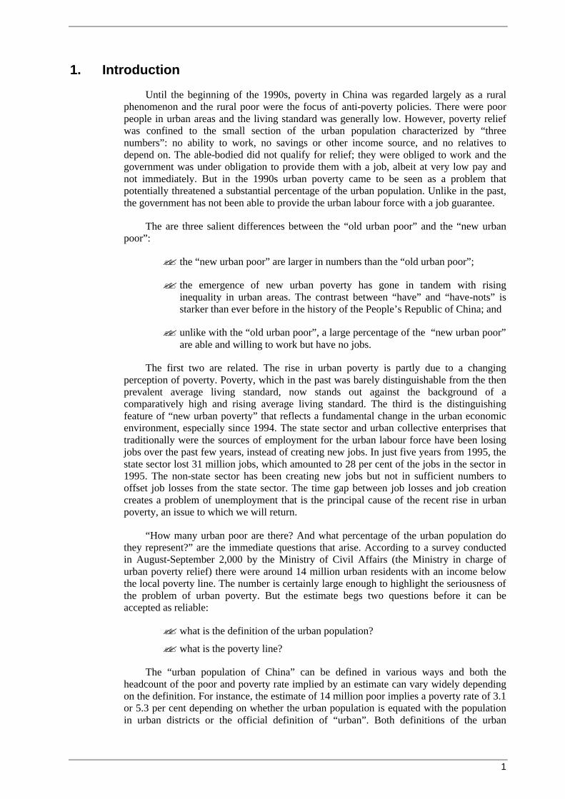
Abbreviations

MOCA Ministry of Civil Affairs

NSB National Statistics Bureau

MLSS Minimum Living Standard Scheme

GPL General poverty line

FPL Food poverty line

Glossary of terms in Chinese

shi qu urban districts

xian rural counties

nongye agricultural

fei nongye non-agricultural

hu kou personal register

dengji shiye ren yuan registered unemployed

xiagang zhigong “laid-off” employees

vii

Abstract

The paper aims to analyse the magnitude and the incidence by regions and population groups of the newly emergent problem of urban poverty in China. Besides the introduction (Section 1), the paper is divided into six sections. Section 2 deals with issues in compiling a poverty profile for urban China. Section 3 outlines the method and data used to calculate the poverty lines, which are used in Section 4 to estimate urban poverty. Section 5 analyses changes in the urban labour market and their implications for poverty and Section 6 assesses the income maintenance schemes. The paper ends with concluding remarks (Section 7).

1

1. Introduction

Until the beginning of the 1990s, poverty in China was regarded largely as a rural phenomenon and the rural poor were the focus of anti-poverty policies. There were poor people in urban areas and the living standard was generally low. However, poverty relief was confined to the small section of the urban population characterized by “three numbers”: no ability to work, no savings or other income source, and no relatives to depend on. The able-bodied did not qualify for relief; they were obliged to work and the government was under obligation to provide them with a job, albeit at very low pay and not immediately. But in the 1990s urban poverty came to be seen as a problem that potentially threatened a substantial percentage of the urban population. Unlike in the past, the government has not been able to provide the urban labour force with a job guarantee.

The are three salient differences between the “old urban poor” and the “new urban poor”:

?? the “new urban poor” are larger in numbers than the “old urban poor”;

?? the emergence of new urban poverty has gone in tandem with rising inequality in urban areas. The contrast between “have” and “have-nots” is starker than ever before in the history of the People’s Republic of China; and

?? unlike with the “old urban poor”, a large percentage of the “new urban poor” are able and willing to work but have no jobs.

The first two are related. The rise in urban poverty is partly due to a changing perception of poverty. Poverty, which in the past was barely distinguishable from the then prevalent average living standard, now stands out against the background of a comparatively high and rising average living standard. The third is the distinguishing feature of “new urban poverty” that reflects a fundamental change in the urban economic environment, especially since 1994. The state sector and urban collective enterprises that traditionally were the sources of employment for the urban labour force have been losing jobs over the past few years, instead of creating new jobs. In just five years from 1995, the state sector lost 31 million jobs, which amounted to 28 per cent of the jobs in the sector in 1995. The non-state sector has been creating new jobs but not in sufficient numbers to offset job losses from the state sector. The time gap between job losses and job creation creates a problem of unemployment that is the principal cause of the recent rise in urban poverty, an issue to which we will return.

“How many urban poor are there? And what percentage of the urban population do they represent?” are the immediate questions that arise. According to a survey conducted in August-September 2,000 by the Ministry of Civil Affairs (the Ministry in charge of urban poverty relief) there were around 14 million urban residents with an income below the local poverty line. The number is certainly large enough to highlight the seriousness of the problem of urban poverty. But the estimate begs two questions before it can be accepted as reliable:

?? what is the definition of the urban population?

?? what is the poverty line?

The “urban population of China” can be defined in various ways and both the headcount of the poor and poverty rate implied by an estimate can vary widely depending on the definition. For instance, the estimate of 14 million poor implies a poverty rate of 3.1 or 5.3 per cent depending on whether the urban population is equated with the population in urban districts or the official definition of “urban”. Both definitions of the urban

2

population have their particular deficiencies and both exclude a large number of migrants working and living in cities who face a greater risk of falling below the urban poverty line than permanent residents. As for the urban poverty line, this can vary depending on locality and what it is used for. Given the almost exclusive focus on rural poverty over a decade and half, there was until the second half of the 1990s - since the beginning of economic reforms, neither an urban poverty line nor any attempt at estimating the headcount of the urban poor.

The paper is structured as follows. Section 2 is a ground clearing operation, dealing with the basic issues that arise in compiling a poverty profile for urban China, including the urban-rural division, the status of migrants and the urban poverty lines that are in use. Section 3 outlines the method and data used to calculate the urban poverty lines, which are used later in Section 4 to estimate urban poverty, its rate and regional pattern. Section 5 presents an analysis of changes in the urban labour market and its implication for urban poverty. Section 6 assesses the income maintenance schemes for unemployed workers and those below the local poverty line. Section 7 is the conclusion.

2. Divisions of the urban population and poverty lines

The Chinese population is divided along two lines, first, urban-rural and, second, permanent residents-migrants. These divisions are founded in the government control on population movement that dates back to the 1950s and still survives, though considerably reduced in rigour. For the present purposes these divisions matter for two reasons. First, as we shall see below, the rural and urban poverty lines are wide apart. Whether a person is regarded as poor depends crucially on the status of the person as urban or rural. Second, the social security cover is very different for the rural and urban population and generally migrants are excluded from social security schemes, regardless of the time since arrival.

2.1 Urban-rural division

In year 2000, the ratio of urban and rural Chinese population was 36:64, and changed from a ratio of 31:69 only a year earlier in 1999. The five-percentage point jump in the share of the urban population in just one year was not caused by a massive surge in exodus from the countryside to cities but by a change in classification. This leads on to the peculiarities of the urban-rural division in China.

Though not very precise, the conventional definition of “urban” refers jointly to a high population density, on the one hand, and industry and services accounting for most of local income on the other. Further, under the usual classification the population resident in an urban locality is regarded as all urban and similarly for rural localities. That is, the spatial division “urban-rural” coincides with the demographic division of the population in urban and rural. In contrast, in China the spatial and the demographic divisions do not coincide and create anomalies. Spatially, Chinese cities divide into urban districts (shi qu) and rural counties (xian). Paralleling this, the population is classified by the personal registration status into “agricultural (nongye)” and “non-agricultural (fei nongye)”, which is what the official category “urban” refers to. The spatial and the demographic divisions overlap, but only partially.

3

Of the 430 million individuals with “non-agricultural registration” (thus officially urban) in 1999,1 37.2 per cent (160 million) were resident in rural counties, not in urban districts.

On the other hand, around 38.6 per cent of long-term residents of urban districts (101 million) carried agricultural registration and were thus regarded as part of the rural population, even though most of these no longer had any relation with farming. They were still classified as "agricultural" because occupational shift from farming to industry and services does not automatically lead to a change in registration from “agricultural” to “non-agricultural”.

The official designation “urban” in China does not denote usual place of residence, such as urban districts of cities, but the label “non-agricultural” (fei nongye) on the personal register (hu kou). That is, “urban” is a personal attribute not a spatial designation. A striking example of this is provided by a comparatively common anomaly in China where some members of a household in an urban district are registered as “non-agricultural”, thus regarded as “urban”, while the rest are regarded as “rural” on the grounds of their registration as “agricultural”. A frequent cause of such anomalies is marriage across the registration line. Urban registration, if not inherited from the mother, is difficult to acquire, especially for large cities such as Beijing and Shanghai.

The 64 per cent of the total population classified as rural in China is oddly high given that the GDP share of agriculture is a mere 15 per cent. This huge gap reflects the administrative control on rural-to-urban migration dating back to the 1950s. When interpreting rural and urban in the Chinese context, it is therefore important to keep in view that these are administrative categories and fit in loosely with a socio-economic classification. Around 30 per cent of the rural labour force is employed full time in non-farming activities and many of the rural counties around cities derive all but a small percentage of income from non-farming activities and resemble urban conurbation in terms of population density. In terms of the usual socio-economic criteria of population density and sources of livelihood, the percentage of the urban population in China is substantially higher than the official 36 per cent. This raises the question of the impact of a re-classification of the Chinese population into urban and rural in line with the usual criteria on the urban poverty headcount and rate.

2.2 Migrants

Rural-to-urban migration has risen sharply since the mid-1980s thanks to a relaxation of restrictions on travel and the expansion of transport facilities. But changes in the system of household registration have lagged behind the rise in population movement. Changes in the usual place of residence in the household register remains subject to official discretion and do not reflect population movement. The result is the emergence of a large population, known as the “floating population”, that is resident in a locality other than the one recorded as the place of residence in the household register. These migrants form a heterogeneous group. They differ in the length of stay in the current location. Some are visitors or short-term migrants and some have been in the current location for a substantial length of time. Six months is cut-off period used in Chinese statistics to distinguish between short-term and long-term migrants. Correlated with this, migrants differ in their official status. A small percentage of them receive a new household registration and these become indistinguishable from the local population. A proportion of them, usually long-term migrants, are granted temporary household registration, which gives them the right to stay but not the full status of a permanent resident. There is no doubt that for the purposes of

1 The figures for the year 2000 are not available.

4

poverty analysis and social security long-term rural immigrants should be regarded as part of the urban population. In the case of short-term rural immigrants, it is far from obvious whether they should be regarded as part of the urban or rural population. This decision takes on a special importance in the Chinese context because the urban poverty line exceeds the rural poverty line by a very wide margin. The commonly used rural and urban poverty lines are respectively Y635 and Y1,800 per person/year. A person may be poor according to the urban but very well off by the rural line.

Despite the attention devoted to the floating population, the data on migration are variable in quality and coverage. The 1995 mid-census population survey put the total number of all types of migrants at 31.7 million, an estimate that is out-of-date. The population census of 2000 collected data on migrants. When released that would provide a detailed picture of migration. Currently, the most comprehensive data on migration that cover all types of migration are the ones released by the Ministry of Civil Affairs (MOCA). The MOCA data are based on registration rather than on a survey. Migrants are officially required to register. Compliance with this requirement varies with locality and the length of stay and it is likely to be low for short-term migrants, those engaged in casual work and the self-employed. Conversely, the compliance rate is likely to high amongst long-term migrants and those engaged in regular employment because they have a high incentive to register.

According to the MOCA data, the floating population totalled 40.4 million in 1999, which comes to 3.2 per cent of the total population. The data set, which is destination based, covers all provinces, except Tibet, and all of the following three categories of migrants:

?? rural-to-rural;

?? urban-to-urban;

?? rural-to-urban.

The last is the largest component, but not the only one. For the purposes of an analysis of urban poverty, it is the last two categories of migrants, with a city as their destination, which are relevant. Together, these two categories account for around 75 per cent of all migrants.2 The MOCA data set does not distinguish between the three categories of migrants but it has the advantageous feature of providing a classification of migrants by duration since arrival (strictly speaking “registration”) at the destination. The distribution of migrants registered with Civil Affairs Bureaux (the territorial branches of the MOCA) by duration since arrival is presented in Table 1.

Table 1. Distribution of migrants by duration

Duration Number in million (% of total)

Less than 1 month 6.0 (15%)

Between 1-12 months 24.0 (59%)

12 months or more 10.1 (26%)

The MOCA estimate of 40 million migrants is lower than a number of alternative estimates, one of which puts the total at as high as 100 million. However, a simple estimate of the migrants total has little value without a breakdown by duration. There is little doubt that the MOCA data underestimates the actual number of migrants, but in the absence of

2 This is based on the estimate that around 25 per cent of migrations are rural-to-rural.

5

any other data it is impossible to specify the extent of under-estimation with a reasonable degree of reliability.

Assuming that the MOCA data presents a rough picture of the distribution by duration, the interesting feature of Table 1 is that almost three-quarters of migrants have been in the current locality for less than a year. The actual percentage may be even higher than this, given that non-compliance with the registration requirement is likely to be higher among short- than long-term migrants. The principal implication is that the turnover rate among migrants is high, which fits in with their disadvantageous status. In most cities, migrants are restricted to jobs that permanent residents do not want. Such jobs are generally low-paid and temporary or casual. As a result, migrants face a greater risk of being laid-off than permanent residents. Added to this, in the event of unemployment they are not entitled either to unemployment benefit or poverty relief for the urban population. This gives migrants an incentive or forces them to return home upon losing a job or the termination of a labour contract, which is reflected in the prevalence of short-term migrants. The incidence of poverty among migrants in comparison to that among permanent residents is discussed below in Section 4.

2.3 Urban poverty lines in currency

The rising urban unemployment and poverty in the 1990s prompted a number of Chinese organizations to calculate an urban poverty line in terms of expenditure needed for a socially acceptable subsistence. These include the National Statistics Bureau (NSB), MOCA and the Institute of Forecasting of the Chinese Academy of Sciences. The method of calculation varies across organizations and there is as yet no agreed framework for calculation. The national poverty lines currently in use fall in the range of Y1,700 to Y2,400 per year per head and are purely diagnostic, i.e. used only for estimating the number of the urban poor, which, as we shall see below, is highly sensitive to slight shifts in the line.

For the practical purposes of providing social relief or assistance to poor urban households, each city sets its own poverty line (or benefit line). The State Council regulations governing the urban “Minimum Living Standard Scheme” (MLSS) delegate local governments to set poverty lines for their jurisdiction. There are two justifications for decentralising the determination of poverty line. First, prices, the pattern of consumption and average income per capita vary widely across localities. Second, the poverty line determines assistance under the MLSS, which is financed principally by city governments. In principle, cities set the poverty line (benefit line) by the direct method of costing the 20 items of goods and services for basic subsistence (the so-called “the basic needs” approach).3 But there is as yet no detailed national framework to guide local governments in setting the poverty line. Methods vary across cities. Some have set up a special group to set the poverty line. Some cities rely on no more than an informed guess in setting the poverty line. Table 2 presents a broad picture of the benefit lines across cities.

3 These 20 items are listed in the “Circular on Strengthening the Investigation and Control of Prices of Necessary Goods and Services” issued by the State Council in 1994.

6

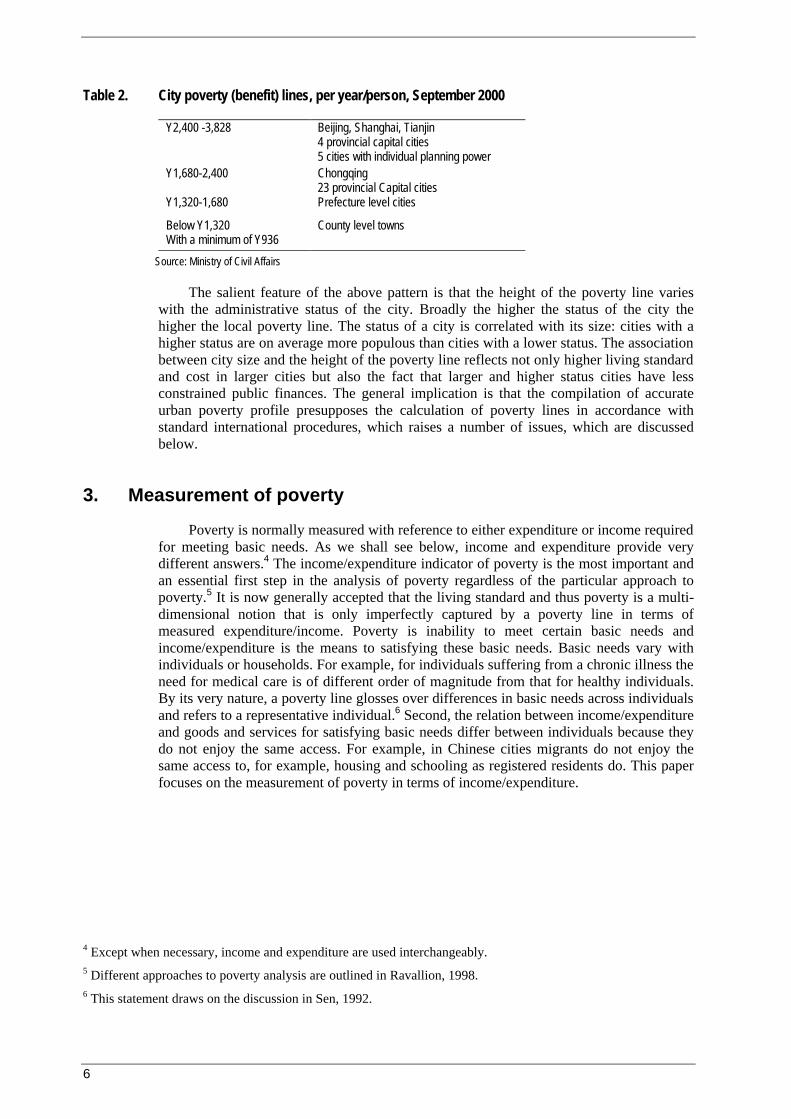
Table 2. City poverty (benefit) lines, per year/person, September 2000

Y2,400 -3,828 Beijing, Shanghai, Tianjin 4 provincial capital cities 5 cities with individual planning power

Y1,680-2,400 Chongqing 23 provincial Capital cities

Y1,320-1,680 Prefecture level cities

Below Y1,320 With a minimum of Y936

County level towns

Source: Ministry of Civil Affairs

The salient feature of the above pattern is that the height of the poverty line varies with the administrative status of the city. Broadly the higher the status of the city the higher the local poverty line. The status of a city is correlated with its size: cities with a higher status are on average more populous than cities with a lower status. The association between city size and the height of the poverty line reflects not only higher living standard and cost in larger cities but also the fact that larger and higher status cities have less constrained public finances. The general implication is that the compilation of accurate urban poverty profile presupposes the calculation of poverty lines in accordance with standard international procedures, which raises a number of issues, which are discussed below.

3. Measurement of poverty

Poverty is normally measured with reference to either expenditure or income required for meeting basic needs. As we shall see below, income and expenditure provide very different answers.4 The income/expenditure indicator of poverty is the most important and an essential first step in the analysis of poverty regardless of the particular approach to poverty.5 It is now generally accepted that the living standard and thus poverty is a multi-dimensional notion that is only imperfectly captured by a poverty line in terms of measured expenditure/income. Poverty is inability to meet certain basic needs and income/expenditure is the means to satisfying these basic needs. Basic needs vary with individuals or households. For example, for individuals suffering from a chronic illness the need for medical care is of different order of magnitude from that for healthy individuals. By its very nature, a poverty line glosses over differences in basic needs across individuals and refers to a representative individual.6 Second, the relation between income/expenditure and goods and services for satisfying basic needs differ between individuals because they do not enjoy the same access. For example, in Chinese cities migrants do not enjoy the same access to, for example, housing and schooling as registered residents do. This paper focuses on the measurement of poverty in terms of income/expenditure.

4 Except when necessary, income and expenditure are used interchangeably. 5 Different approaches to poverty analysis are outlined in Ravallion, 1998. 6 This statement draws on the discussion in Sen, 1992.

7

3.1 Issues in setting poverty lines

It is important to distinguish between the two types of poverty lines on the basis of their uses:

?? diagnostic poverty lines;

?? poverty lines used for poverty relief work (referred to above as the “benefit line”).

Though related, the two are in principle distinct and can be very different. A diagnostic poverty line is purely for the purpose for identifying the poor. While sensitive to the prevalent living standard, it is not constrained by how to provide assistance to those below the poverty line. Such a line can also serve as a benchmark for assessing the adequacy of the existing benefit lines and setting a horizon for poverty alleviation. In contrast, a benefit line serves to identify potential recipients of social assistance and determine the magnitude of assistance. Therefore it is directly affected by considerations that underlie social security schemes. Of particular importance among these are the following two:

?? the fiscal constraint on funding;

?? maintaining the incentive to undertake employment.

In China, both these considerations apply to the benefit line under the MLSS, discussed below. The poverty lines reported here are “diagnostic poverty lines”, the calculation of which raises the following three issues:

?? geographical coverage;

?? adjustment for household size and composition;

?? which poverty lines?

Geographical coverage

The geographical coverage of a poverty line is a central issue in a country such as China covering a territory that is as heterogeneous as it is extensive. One option is to have a line that applies uniformly to the whole urban population regardless of the particular characteristics of the locality, such as the one determined by the NSB. But the value of such lines is greatly diminished by the fact that consumption patterns, prices and prevalent living standards (or per head income) vary as widely across regions in China as they may do across countries. The other option is to have lines that apply to sub-national units, such as provinces or cities and the national line is simply their average. The choice of the geographical units involves a trade-off between more detail and keeping computation within a manageable limit. In the Chinese context, a number of sub-national units for the computation of poverty lines suggest themselves, such as provinces and large or small cities classified by regions. As a first cut, we chose provinces as the unit of calculation. Regional, such as the coastal and interior provinces, and the national poverty lines can be calculated as the weighted averages of respective provincial poverty lines, with weights equal to the provincial shares of the urban population.

The calculation of province-specific instead of uniform national poverty lines makes a substantial difference to the analysis of urban poverty. As shown below, provincial poverty line differs widely. The gap between the lowest and highest poverty line can be 2.5 times or more (see Table 3 below). Some of this difference is due to regional price variations that can be corrected by means of a price index. But a major part is also due to variable consumption patterns associated with differences in the living standard and other factors, which cannot be captured by means of an index. As a result, the use of a uniform poverty

8

line for the whole country will distort the regional pattern of poverty, exaggerating the incidence in some provinces (predominantly interior provinces) and understating in some others (predominantly coastal provinces). The implication is that in the Chinese context a national poverty line is a highly unreliable instrument for identifying targets for anti-poverty policies. Provincial poverty lines also suffer from defects but less so than national poverty lines because variations in consumption pattern within provinces are less pronounced than national variations.

Adjustment for household size and composition

Poverty lines are usually expressed with reference to an individual. But the living standard of individuals depends crucially on the size and age composition of the household of which they are a part, as well as on their income/expenditure per head. This raises the question of adjustment to poverty line, taking into account the household size, if also not the age-composition. In a number of countries, such as those of the European Union and the United States, an equivalence scale is applied to take account of the household size and age-composition. In what is referred to as the OECD scale, the weights are 1 for the first adult, 0.6 for other adults and 0.6 for children. The argument in favour for giving the additional adult a weight less than one is that a number of goods that affect the living standard are consumed jointly rather than individually. Housing and household durable goods are obvious examples of goods that are consumed jointly. As a result, at a given living standard it costs less to support a two-person household than it does to two single-person households. It is well established that controlling for income/expenditure per head, the pattern of consumption depends crucially on the size of the household.

In the calculation of poverty lines we do not use an equivalence scale because in the Chinese context there is no scale that commands general acceptance. The benefit lines in China are not adjusted for household size. A two-person household is treated the same as two single-person households. The question of an equivalence scale does not arise in the case of what is termed below “the food poverty line” because that is calculated with reference to the calorie requirement for a healthy adult, 2,100 calories per day. However, the question of adjustment for household size does arise in the case of basic “non-food expenditure” because that it is calculated not with reference to a fixed norm, such as 2,100 calories per day/person. Rather it is calculated with reference to the non-food items households chose to spend on, controlling for either total or food expenditure (explained below). The choice of the expenditure pattern, in particular the division between food and non-food items, is crucially affected by household size as well as income/expenditure per head. The calculation of the basic non-food expenditure is based on the assumption that the household size is equal to the observed national average of 3.1 persons.

Which poverty lines?

Even in the case of agreement on the poverty indicator, such as household expenditure or income per head, there is room for divergence of views on where the poverty line should be drawn. There are two good arguments in favour of having several poverty lines rather than just one. First, poverty does not denote just one side of a binary division. There is a gradation of poverty ranging from severe to mild and a convenient way of representing this gradation is to have several poverty lines or alternatively to test the sensitivity of poor headcount to shifts in a poverty line. Second, income or expenditure is always measured with a margin of error because of either mis-measurement or unrecorded components. This suggests the importance of testing the sensitivity of the incidence of poverty, as for example measured by the headcount of the poor, to a shift in the poverty line. In this paper we report for each of the 31 provinces two sets of poverty lines: food poverty line and general poverty lines (hereafter referred to as the “poverty line”). In addition, to indicate the sensitivity of the poverty incidence to a shift in poverty line, in Section 4 we report poverty rates for various multiples of the poverty line.

9

Another major issue in the computation of poverty lines is the choice between “absolute” and “relative” poverty lines. The meaning of these two terms varies in the literature. Here “absolute” and “relative” are defined with reference to the procedure of determining the line.7 An absolute poverty line is taken here to denote a poverty line that is defined in terms of the cost of a specified basket of food and non-food items that has some justification as the minimum “necessary” or as representing basic needs. In contrast, a relative poverty line is taken here to denote a poverty line that is not tied down to goods and services, but to average expenditure or income in the reference locality. A simple example is a line set as a percentage of the average, which can be either the arithmetic mean or the median. The “absolute” and “relative” poverty lines are not mutually exclusive. There are contexts in which an absolute line is more appropriate than the relative line and vice-versa. There is an undeniable “absolute” core to poverty, especially when the concern is with nutrition. It may be argued that “absolute” poverty is primary in the sense its alleviation takes precedence over the alleviation of “relative” poverty, especially in a developing economy where a fixed percentage of average income/expenditure may not be sufficient to meet even bare minimum needs. In many poor rural localities in Western China everyone may be absolutely poor, while none may be relatively poor.8 A relative poverty line is appropriate only in those situations where the average income/expenditure far exceeds the absolute poverty line and in situations where ensuring basic requisites of life for all is not the pressing concern.

The poverty lines presented in this paper are all “absolute” poverty lines in the sense that they are anchored to the notion of basic necessities. These lines vary across provinces and are, in principle, variable over time, but are not relative in the sense they are not set with reference to average income/expenditure. However, these can be used as benchmarks for setting “relative” poverty lines.

3.2 Two poverty lines

The following two sets of poverty lines are computed for each of the 31 Chinese provinces and also for the whole of China:

?? food poverty line;

?? general poverty line.

The general poverty line is regarded as the sum of two components: basic food expenditure, as given by the food poverty line, and basic non-food expenditure, which, as explained below, can be calibrated in various ways.

Food poverty line

The food poverty line is a popular method of setting poverty lines in developing economies where adequate nutrition is the first priority of poverty alleviation. The first step in the calculation of a food poverty line is the choice of the indicator of adequate nutrition. A variety of indicators are possible, such as number of full meals per day or food energy intake. The latter is chosen because, compared to others, it lends itself to measurement more easily and can be set with reference to requirements for healthy living. Nutritionists have formulated lists of nutrients conducive to a healthy life. The most important of these nutrients is calorie. Generally, adequate calorie intake is associated with an adequate intake of the other principal nutrient, protein. As pointed out by nutritionists,

7 This characterisation of “absolute” and “relative” poverty lines relies on Atkinson’s 1998 “Poverty in Europe”. 8 A forceful case for retaining the notion of absolute poverty is provided in Sen, 1983.

10

the minimum calorie requirement for a healthy person can vary widely with gender, age, physical activity and climate. For the purposes of setting a poverty line for the whole population, it is useful to choose a calorie level that applies to a substantial percentage of the population and is no less than the levels that apply to most other sections of the population. Following the literature on poverty and nutrition this is taken to be 2,100 calories per day per person.9

The calorie standard is only a benchmark and on its own insufficient to determine the food poverty line. A huge number of food baskets are able to provide the daily calorie requirement of 2,100. But many of these are not acceptable on the ground of either being alien to the prevalent dietary pattern or not cost effective. Apart from satisfying the calorie requirement, the food basket underpinning the food poverty line has to satisfy the following additional conditions:

?? should fit in with the local dietary pattern;

?? should be cost-effective.

These conditions are satisfied by choosing the contents of the food basket with reference to the average per head consumption of various food items by the first quintile (the bottom 20 per cent) of the sampled households in the province in question ranked by expenditure per head, excluding expenditure on consumer durables. The choice of the bottom 20 per cent as the reference percentile is based on two considerations. The first is that it should include all poor households as well as those on the margin. Second, it should have enough households to smooth out variations across households that are not directly related to income/expenditure. The reason for excluding durables is that they are purchased at irregular intervals and thus introduce a white noise in the relation between current consumption and current living standard. The basket thus chosen obviously represents the local (provincial) dietary pattern and is also cost effective. The latter because the bottom 20 per cent represents low income/expenditure households and such households use cheaper food to acquire necessary calories. The calorie content of the basket is calculated by multiplying physical quantities of food items, which is provided by the NSB urban survey data, with their respective calorie content from the physical quantity-nutrients table compiled by the Nutrition Society of China.10 To meet the requirement of 2,100 per day, the basket is scaled up or down depending upon the case. In effect the calorie requirement functions as a scaling factor that can be varied depending on the purpose.

The cost of the chosen food basket is obtained automatically because the NSB urban household data provides for a long list of food items both the physical amount purchased (where applicable) and the total expenditure on each item. The advantage of calculating costs in this way is that the cost is automatically adjusted for the prices actually paid by the household and the quality of purchased items. Aside from serving as the “food poverty line”, the cost of the minimum calories requirement can also serve as the provincial price index11 that is a more accurate index of the cost of living than the urban price index reported in published statistics. It is important to emphasise that although the food poverty line can be used to estimate severe poverty, it is on its own insufficient. The line only covers the cost of purchasing uncooked food and excludes all non-food expenditure including that incurred in cooking food.

9 If the concern is with “under-nutrition” then the focus should be on a wider range of nutrients than calories alone and on the intake relative to the requirement adjusted for physiological characteristics. 10 This involves excluding those food items for which no physical quantities are reported. These usually consist of meals outside home. 11 Strictly speaking, not a price index but a unit-value index.

11

An alternative way of determining the basic food expenditure is by means of the share of total expenditure devoted to food. Following Engel, the food share is taken as the indicator of the living standard and on the basis of an empirical observation a particular share is chosen as the marker of poverty. The threshold share varies but is generally greater than 50 per cent. The NSB uses 60 per cent. With the threshold share given, the food poverty line is given by the average food expenditure per head when it is just equal to the chosen percentage, for example 60 per cent, of income/total expenditure per head. The method makes intuitive sense and is easy to implement. It needs no more statistical data than the broad division of expenditure into “food” and “non-food” items. Though valuable for a quick reckoning, the method is defective and can mislead. The food share depends not only on income/total expenditure per head, which is the variable of interest in the determination of a poverty line, but also on relative prices between food and non-food items and the household size. Comparing two localities, a high food share may simply represent a relatively high food price rather than a low living standard. Further, it is generally the case that, with income/total expenditure held constant, larger households have a smaller food share than do smaller families. The reason is less that larger households benefit from economies of scale in food consumption but more that they spend more on durables and housing, goods that are consumed jointly rather than individually.12 The implication is that as the indicator of the living standard, the food share exaggerates the living standard of larger households and of households faced with a higher relative price of non-food items.

General poverty lines

Given the food poverty line, the next issue is to determine the basic “non-food expenditure” per head so as to obtain a general poverty line. The “non-food” items cover a diverse range and there is no simple standard to serve as the benchmark for deciding the basic minimum calories per person/day in the case of food consumption. There are various possibilities for determining basic non-food expenditure per head and these can be divided into two types: direct and indirect. The direct one is to calculate the cost of various non-food items specified with reference to the standard for each category of goods and services such as clothing, housing, energy consumption etc. This approach, although valuable, is insufficient in the sense it leaves a large category of miscellaneous non-food expenditure that can neither be excluded as “unnecessary” nor can be specified in terms of a physical standard. The only way of accounting for such expenditure is in terms of a monetary sum that can be justified as being necessary.

The other approach is indirect and consists in setting the basic non-food expenditure at a level just consistent with maintaining the food expenditure at the basic level. The NSB calculates the “basic non-food expenditure” by setting it equal to 40 per cent of the total expenditure when the food share is 60 per cent. This is equivalent to assuming that at the poverty line the basic non-food expenditure is equal to two-third of the “basic food expenditure”. We also use the indirect approach for calculating “basic non-food expenditure” with reference to the food poverty line, but with reference to one determined on the basis of the calorie requirement, not the food share. Answering the following question by means of a regression exercise on the urban household data sets the “basic non-food expenditure” per head.

??What is the non-food expenditure per head when expenditure per head on food just hits the food poverty line?

12 A detailed criticism of the use of food share as an unambiguous indicator of the living standard is provided in Deaton’s (1997) “The Analysis of Household Surveys: A Microeconometric Approach”.

12

The regression equation is explained in appendix 1 of this paper.13 The basic non-food expenditure is defined as the expenditure consistent with maintaining the food expenditure at the food poverty line.

It is necessary to specify the household size in order to determine the “basic non-food expenditure” per person. In the calculations here, we set the household size equal to the national average in urban areas, which is 3.1 persons. Just as the food poverty line is set with reference to the calorie requirement for an average person, the “basic non-food expenditure” is determined with reference to an average size household. Given the estimate of the impact of household size on the division of expenditure between food and non-food items from the regression, it is easy to recalculate the “basic non-food” expenditure for different household sizes. How does the “basic non-food expenditure” per person vary with the household size? According to regression estimate, holding total expenditure constant, the expenditure share of non-food item rises with an increase in household size. That is, the basic non-food expenditure per head increases with household size.

3.3 Data used for calculating urban poverty line

The findings on urban poverty reported here are based on the data from the 1998 urban household survey conducted by the National Statistics Bureau (the NSB survey data). The sample size is 17,000 households, drawn from all 31 provinces according to a multi-stage stratified sampling frame.14 Stratification ensures a wide coverage of the sample that is very small relative to the population it represents. In all, the sample covers 146 out of 668 cities and 80 out of 1,700 rural county seats. The NSB survey aims to serve a variety of uses and is not specifically designed to measure poverty. Whatever shortcomings it may have in this respect, these are more than compensated by the fact that the survey provides by far the most comprehensive coverage of the urban population.

By design, the sample excludes the long-term residents of urban districts with agricultural registration but includes residents of rural counties with non-agricultural registration. The implication is that the data sample is a biased sample of the urban-district population, which is the object of interest here. It includes some of those who should be excluded, residents of rural counties, and excludes some of those who should be included, long-term residents of urban districts. To a degree it is possible to correct this bias by supplementing the findings based on the usual NSB data set with the picture of poverty among long-term migrants derived from the occasional survey of the urban population conducted in 1999 that includes migrants.

In the NSB data set there are 1,500 entries for each household including details of household composition, income and expenditure. Data on income include sources, taxes, transfers and saving and dis-saving. Data on expenditure include a detailed breakdown of expenditure by items and, where relevant, physical quantity purchased. In particular, data on food expenditure is detailed enough for a fairly precise calculation of the calorie content of the food purchased by the household, which is what we use to calculate the food poverty line.

13 The procedure draws on Ravallion’s (1994) “Poverty Comparisons”. 14 The original sample consists of 40,000 households, from which a sub-sample of 17,000 is drawn.

13

3.4. Estimated poverty lines

Table 3 presents the following two lines estimated from the 1998 urban household data for each of the 31 provinces and for whole country in terms of Rmb per head per year:

?? food poverty line;

?? general poverty line.

The national poverty line is a weighted average of the corresponding provincial poverty lines15 and is useful as a benchmark for a cross-comparison of provincial lines and for an assessment of various national poverty lines for urban areas that are currently in use. However, as shown below, a national poverty line is a distorting yardstick for estimating poverty incidence. Column 4 of Table 3 presents the percentage ratio of the food poverty line to the “general poverty line”. This gives the share of food expenditure at the higher poverty line for all provinces, which is used below to analyse the implications of fixing the provincial poverty line with reference to a given value of the food share, such as 60 per cent used by the NSB.

There are two features that stand out in Table 3:

?? For both variants of poverty lines, provincial lines vary very widely, as indicated by the figures in the brackets that express provincial poverty lines as a percentage of the national line.

?? The ratio of the food poverty line to the general poverty line, which gives the food share of those at the poverty line, also varies widely.

The first reinforces the case for using provincial lines in preference to a uniform national line for measuring poverty. The second feature brings to light the implication of defining poverty in terms of food share, discussed below. Focusing on the higher poverty line, what are the consequences of using the uniform national line across all provinces? Apart from three exceptions, the coastal provinces have a poverty line higher than the national average and the interior provinces lower. The three exceptions are: Yunnan, an interior province with a poverty line of 102 per cent of the national average, and Liaoning and Jiangsu, coastal provinces with poverty lines of 95.4 per cent and 96.5 per cent of the national average respectively. The general implication of the pattern is that a single line would understate poverty in the coastal provinces and correspondingly exaggerate poverty in the interior provinces. The net effect would be a highly distorted picture of poverty incidence across provinces. It is not possible to indicate the direction of the bias a priori because that depends on the distribution of households by income/expenditure per head in each province.

15 The weights are equal to provincial shares of the total regional or national urban population depending on the case.

14

Table 3. Estimated poverty lines

Food Poverty Line (FPL) (%, National Line)

(1)

General Poverty Line (GPL) (%, National Line)

(2)

%, FPL/GPL (%, National Ratio)

(3) Beijing 1 983 (142.5%) 3 118 (135.0%) 63.6 (105.5%)Tianjin 1 728 (124.1%) 2 993 (129.6%) 57.7 (95.7%)Hebei 1 336 (96.0%) 2 509 (108.6%) 53.2 (88.3%)Shanxi 960 (69.0%) 1 616 (70.0%) 59.4 (98.5%)Inner Mongolia 1 008 (72.4%) 1 824 (79.0%) 55.3 (91.6%)Liaoning 1 259 (90.4%) 2 203 (95.4%) 57.1 (94.8%)Jilin 1 051 (75.5%) 1 831 (79.3%) 57.4 (95.2%)Heilongjiang 1 071 (76.9%) 1 878 (81.3%) 57.0 (94.6%)Shanghai 2 361 (169.6%) 3 636 (157.3%) 64.9 (107.7%)Jiangsu 1 448 (104.0%) 2 228 (96.5%) 65.0 (107.8%)Zhejiang 1 824 (131.0%) 2 989 (129.4%) 61.0 (101.2%)Anhui 1 319 (94.8%) 2 138 (92.6%) 61.7 (102.3%)Fujian 1 554 (111.6%) 2 416 (104.6%) 64.3 (106.7%)Jiangxi 1 164 (83.6%) 1 809 (78.3%) 64.3 (106.7%)Shandong 1 308 (94.0%) 2 566 (111.1%) 51.0 (84.5%)Henan 1 076 (77.3%) 1 904 (82.4%) 56.5 (93.7%)Hubei 1 354 (97.3%) 2 283 (98.8%) 59.3 (98.4%)Hunan 1 277 (91.7%) 2 146 (92.9%) 59.5 (98.7%)Guangdong 2 083 (149.6%) 3 061 (132.5%) 68.0 (112.9%)Guangxi 1 572 (112.9%) 2 507 (108.5%) 62.7 (104.0%)Hainan 1 693 (121.6%) 2 465 (106.7%) 68.7 (113.9%)Sichuan 1 259 (90.4%) 2 004 (86.8%) 62.8 (104.2%)Guizhou 1 341 (96.3%) 2 137 (92.5%) 62.8 (104.1%)Yunnan 1 484 (106.6%) 2 359 (102.1%) 62.9 (104.3%)Tibet 1 456 (104.6%) 2 237 (96.8%) 65.1 (107.9%)Chongqing 1 355 (97.3%) 2 214 (95.8%) 61.2 (101.5%)Shaanxi 1 080 (77.6%) 2 014 (87.2%) 53.6 (88.9%)Gansu 1 127 (81.0%) 1 819 (78.7%) 62.0 (102.7%)Qinghai 941 (67.6%) 1 484 (64.2%) 63.4 (105.2%)Ningxia 1 085 (77.9%) 2 093 (90.6%) 51.8 (86.0%)Xinjiang 1 117 (80.2%) 1 772 (76.7%) 63.0 (104.5%)National 1 392 (100.0%) 2 310 (100.0%) 60.3 (100.0%)

4. Urban poverty profile

4.1 Identifying the urban poor

A household is poor if it falls below the poverty line, but it can do so in two different ways:

?? either its income per head is lower than the poverty line

?? or its expenditure per head is lower than the poverty line.

The time patterns of income and expenditure diverge. For any given time period, for example a year, income per head would be different from expenditure per head in most households, including those with a low income. As a consequence, the headcount of the poor would differ, possibly by a wide margin, depending on whether income or

15

expenditure per head is used as the poverty indicator. The difference between income and expenditure over a period such as a year consists in net savings. If a household has a positive net saving then its income will exceed its expenditure. As a result, it may be above the poverty line in terms of its income per head but below in terms of its expenditure per head. Conversely, when a household has a negative net savings then it may be below the poverty line in terms of income per head but above in terms of expenditure per head. The net impact of the choice of income or expenditure head on the headcount of the poor and the poverty depends crucially on the balance between savers and dis-savers amongst low-income households.

There are arguments both for and against using either income or expenditure per head as the identifier of the poor. Neither side is decisive enough to rule out the alternative. The argument in favour of using income per head is that it indicates whether the household is financially capable of financing the expenditure indicated by the poverty line without resorting to borrowing, an option that may not be available. This fits in with means testing which is concerned with resources at the disposal of households not with how they actually use their resources. For the purposes of poverty alleviation, the incidence of poverty in terms of income per head is more relevant than that in terms of expenditure per head. The reason is that such a policy is usually aimed at altering income per head in the first instance and influencing expenditure only indirectly. However, there are instances where policy may be more concerned with expenditure, such as that on schooling or healthcare, and less with income per head.

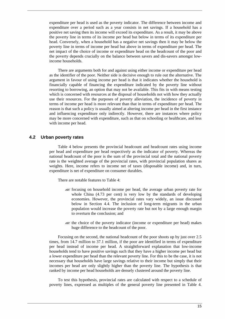
4.2 Urban poverty rates

Table 4 below presents the provincial headcount and headcount rates using income per head and expenditure per head respectively as the indicator of poverty. Whereas the national headcount of the poor is the sum of the provincial total and the national poverty rate is the weighted average of the provincial rates, with provincial population shares as weights. Here, income refers to income net of taxes (disposable income) and, in turn, expenditure is net of expenditure on consumer durables.

There are notable features to Table 4:

?? focusing on household income per head, the average urban poverty rate for whole China (4.73 per cent) is very low by the standards of developing economies. However, the provincial rates vary widely, an issue discussed below in Section 4.4. The inclusion of long-term migrants in the urban population would increase the poverty rate but not by a large enough margin to overturn the conclusion; and

?? the choice of the poverty indicator (income or expenditure per head) makes huge difference to the headcount of the poor.

Focusing on the second, the national headcount of the poor shoots up by just over 2.5 times, from 14.7 million to 37.1 million, if the poor are identified in terms of expenditure per head instead of income per head. A straightforward explanation that low-income households tend to have positive savings such that they have a higher income per head but a lower expenditure per head than the relevant poverty line. For this to be the case, it is not necessary that households have large savings relative to their income but simply that their incomes per head are only slightly higher than the poverty line. The hypothesis is that ranked by income per head households are densely clustered around the poverty line.

To test this hypothesis, provincial rates are calculated with respect to a schedule of poverty lines, expressed as multiples of the general poverty line presented in Table 4.

16

Table 5 presents a summary picture in terms of the national poverty rate (a weighted average of the provincial rates).

Table 4. Urban poverty patterns, 1998

Headcount of the poor Poverty rate Income p/h

(1) Expenditure p/h

(2)

% Ratio (1)/(2)

(3) Income p/h

(4) Expenditure p/h

(5) Beijing 54 000 422 000 773 0.73 5.64 Tianjin 360 000 969 000 269 6.77 18.23 Hebei 651 000 2 010 000 308 5.20 16.04 Shanxi 596 000 1 637 000 275 7.17 19.69 Inner Mongolia 510 000 1 778 000 348 6.40 22.3 Liaoning 1 150 000 2 383 000 207 6.13 12.7 Jilin 853 000 1 295 000 152 7.54 11.44 Heilongjiang 1 154 000 2 743 000 238 6.92 16.46 Shanghai 314 000 584 000 186 3.24 6.02 Jiangsu 244 000 1 298 000 533 1.20 6.4 Zhejiang 153 000 463 000 302 1.62 4.89 Anhui 348 000 1 060 000 304 2.89 8.8 Fujian 145 000 319 000 219 2.18 4.78 Jiangxi 310 000 1 261 000 407 3.42 13.92 Shandong 1 172 000 4 689 000 400 5.05 20.19 Henan 1 410 000 3 088 000 219 8.39 18.38 Hubei 934 000 1 763 000 189 5.67 10.71 Hunan 462 000 1 336 000 289 3.61 10.44 Guangdong 154 000 244 000 157 0.68 1.07 Guangxi 246 000 620 000 252 3.01 7.59 Hainan 150 000 418 000 278 7.94 22.09 Sichuan 711 000 1 102 000 155 4.72 7.31 Guizhou 260 000 864 000 333 5.00 16.65 Yunnan 225 000 595 000 264 3.69 9.73 Tibet 39 000 65 000 168 11.31 19.05 Chongqing 260 000 548 000 211 4.09 8.62 Shaanxi 932 000 1 567 000 168 11.95 20.08 Gansu 304 000 792 000 260 6.44 16.77 Qinghai 76 000 131 000 173 5.63 9.76 Ningxia 210 000 403 000 192 13.51 25.91 Xinjiang 383 000 625 000 163 6.16 10.06 Whole China 14 770 000 37 072 000 251 4.73 11.87

Table 5. Sensitivity of the poverty rate to shifts in poverty line

Poverty line as multiple of the general poverty line (GPL) National poverty rate %

0.75* GPL 1.38

0.85* GPL 2.42

1.00 GPL 4.73

1.15* GPL 8.17

1.25* GPL 11.07

1.35* GPL 14.40

1.5* GPL 20.08

2* GPL 41.10

17

The striking feature of Table 5 is the very large changes in response to comparatively small shifts in the poverty line. An increase of the national poverty line by 15 per cent (denoted by 1.15*GPL in Table 5) raises the national poverty rate by as much as 72.7 per cent from 4.7 to 8.2 per cent of the urban population. Raising the poverty line by another 10 percent (denoted by 1.25*GPL) raises the national poverty rate by 43.2 per cent from 8.2 to 11.1 per cent of the urban population. The latter poverty rate is close to the poverty rate when expenditure instead of income per head is used as the indicator. This indicates that in term of impact on the national poverty rate, the change in the indicator from income to expenditure is equivalent to raising the poverty line by just over 25 per cent, while keeping income per head as the indicator of poverty.

What are the policy implications of the acute sensitivity of the poverty rate to a comparatively small shift in the poverty line, which also happens to be true of the rural poverty profile? A salient implication is that a significant percentage of the non-poor urban population remains highly susceptible to a fall into poverty as a result of a relatively small reduction in income or, for example, a rise in non-food expenditure as a result of illness. The latter is equivalent to a reduction in income in the sense that the affected household is forced to cut expenditure either on food or on non-food items. This suggests that the focus of poverty alleviation measures should not be confined to those who fall below the poverty line, it should also extend to the population with a high risk of falling into poverty. The appropriate policy response with respect to the latter group is not social assistance but increasing the capability of low-income households to cope with risks, by, for example, provision of health insurance against serious illness. The vulnerability of a substantial percentage of the urban population falling into poverty as a result of relatively small decrease in household income per head also emphasises the importance of a social safety net that covers all urban population rather than, as in the past and still so in practice, a small section of the population with no ability to work, no savings and no relatives to depend on.

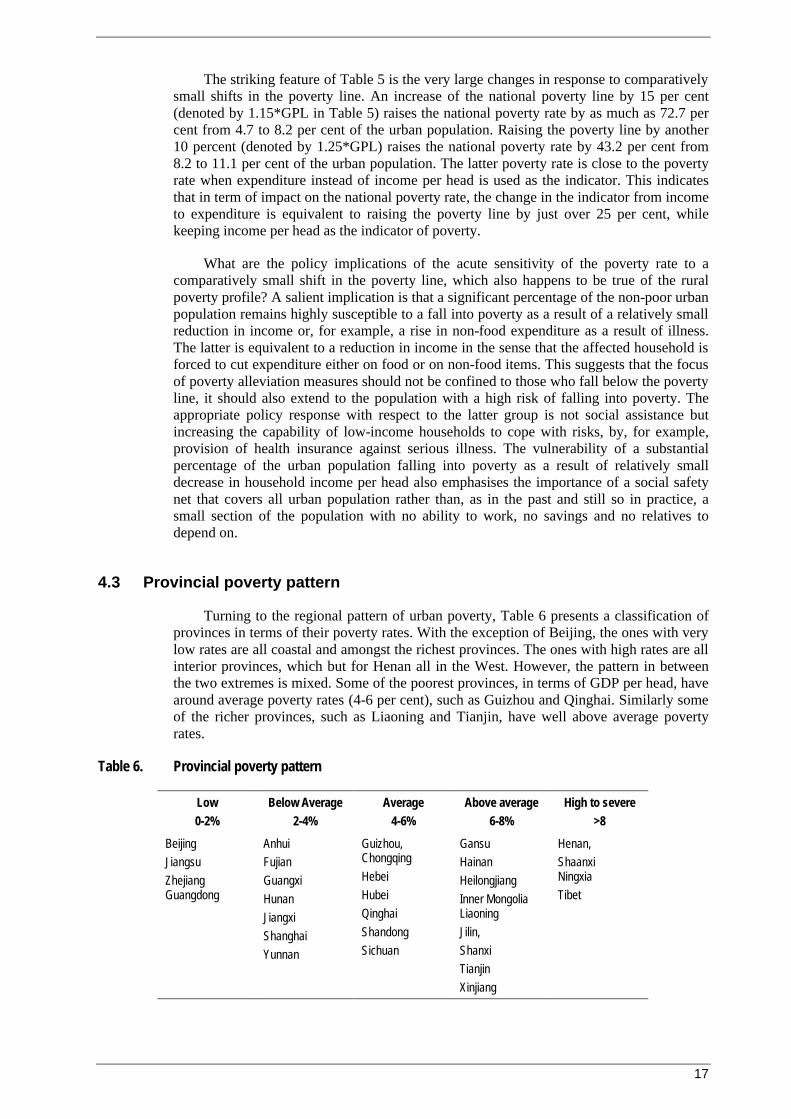
4.3 Provincial poverty pattern

Turning to the regional pattern of urban poverty, Table 6 presents a classification of provinces in terms of their poverty rates. With the exception of Beijing, the ones with very low rates are all coastal and amongst the richest provinces. The ones with high rates are all interior provinces, which but for Henan all in the West. However, the pattern in between the two extremes is mixed. Some of the poorest provinces, in terms of GDP per head, have around average poverty rates (4-6 per cent), such as Guizhou and Qinghai. Similarly some of the richer provinces, such as Liaoning and Tianjin, have well above average poverty rates.

Table 6. Provincial poverty pattern

Low 0-2%

Below Average 2-4%

Average 4-6%

Above average 6-8%

High to severe >8

Beijing Jiangsu Zhejiang Guangdong

Anhui Fujian Guangxi Hunan Jiangxi Shanghai Yunnan

Guizhou, Chongqing Hebei Hubei Qinghai Shandong Sichuan

Gansu Hainan Heilongjiang Inner Mongolia Liaoning Jilin, Shanxi Tianjin Xinjiang

Henan, Shaanxi Ningxia Tibet

18

Turning to the salient features of the regional pattern of urban poverty, there are various ways of grouping Chinese provinces. The two common ones are:

?? three part division into “Coastal”, “Central” and “Western”;16 and

?? six-region division into “North”, “North-East”, “East”, “South-East”, “South-West” and “North-West”.17

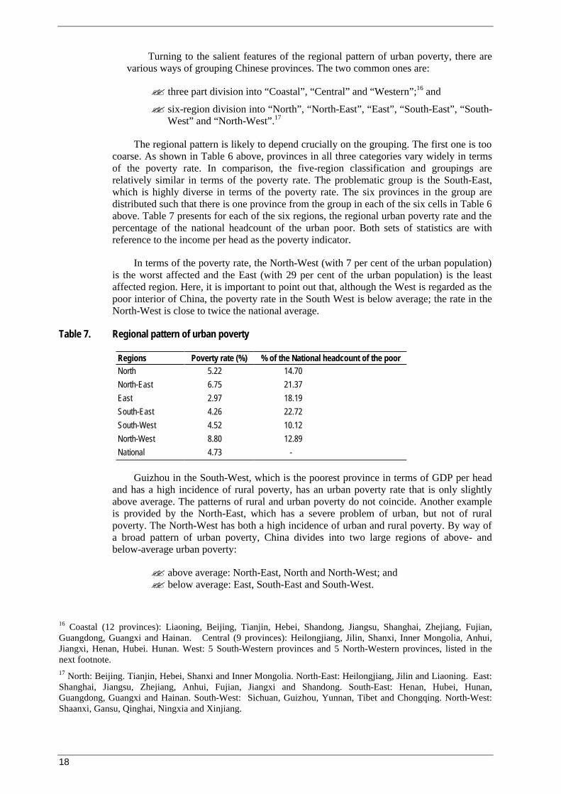
The regional pattern is likely to depend crucially on the grouping. The first one is too coarse. As shown in Table 6 above, provinces in all three categories vary widely in terms of the poverty rate. In comparison, the five-region classification and groupings are relatively similar in terms of the poverty rate. The problematic group is the South-East, which is highly diverse in terms of the poverty rate. The six provinces in the group are distributed such that there is one province from the group in each of the six cells in Table 6 above. Table 7 presents for each of the six regions, the regional urban poverty rate and the percentage of the national headcount of the urban poor. Both sets of statistics are with reference to the income per head as the poverty indicator.

In terms of the poverty rate, the North-West (with 7 per cent of the urban population) is the worst affected and the East (with 29 per cent of the urban population) is the least affected region. Here, it is important to point out that, although the West is regarded as the poor interior of China, the poverty rate in the South West is below average; the rate in the North-West is close to twice the national average.

Table 7. Regional pattern of urban poverty

Regions Poverty rate (%) % of the National headcount of the poor North 5.22 14.70

North-East 6.75 21.37

East 2.97 18.19 South-East 4.26 22.72

South-West 4.52 10.12

North-West 8.80 12.89 National 4.73 -

Guizhou in the South-West, which is the poorest province in terms of GDP per head and has a high incidence of rural poverty, has an urban poverty rate that is only slightly above average. The patterns of rural and urban poverty do not coincide. Another example is provided by the North-East, which has a severe problem of urban, but not of rural poverty. The North-West has both a high incidence of urban and rural poverty. By way of a broad pattern of urban poverty, China divides into two large regions of above- and below-average urban poverty:

?? above average: North-East, North and North-West; and ?? below average: East, South-East and South-West.

16 Coastal (12 provinces): Liaoning, Beijing, Tianjin, Hebei, Shandong, Jiangsu, Shanghai, Zhejiang, Fujian, Guangdong, Guangxi and Hainan. Central (9 provinces): Heilongjiang, Jilin, Shanxi, Inner Mongolia, Anhui, Jiangxi, Henan, Hubei. Hunan. West: 5 South-Western provinces and 5 North-Western provinces, listed in the next footnote. 17 North: Beijing. Tianjin, Hebei, Shanxi and Inner Mongolia. North-East: Heilongjiang, Jilin and Liaoning. East: Shanghai, Jiangsu, Zhejiang, Anhui, Fujian, Jiangxi and Shandong. South-East: Henan, Hubei, Hunan, Guangdong, Guangxi and Hainan. South-West: Sichuan, Guizhou, Yunnan, Tibet and Chongqing. North-West: Shaanxi, Gansu, Qinghai, Ningxia and Xinjiang.

19

What are the implications of the regional dimension for targeting urban poverty alleviation measures? The importance of poor individuals and households as policy targets is obvious and does not require special justification. But there is also a case for targeting localities. The case rests on the fact that the causes of poverty are not all specific to individuals. Some causes affect a significant section of the population in the locality. One example of such a cause is the closure of an enterprise employing a substantial percentage of the labour force in the locality, a common occurrence in towns and cities in the North-East and the North-West. Such localities can be caught in a vicious spiral whereby an initial surge in poverty can become a cause of a further rise and perpetuation of urban poverty. Developed economies offer ample examples of such phenomenon, but China seems to be experiencing similar phenomenon of vicious and virtuous spirals of growth and decline of towns and cities.

A crucial question is what is the appropriate level of geographical targeting of urban poverty alleviation policies? Provincial groupings such as those listed in Table 8 are too heterogeneous to be appropriate targets and so too are provinces. The appropriate level is the one where economic interdependence is high and this would seem to be towns and districts of large cities.

4.4 Poverty among migrants

Given the disadvantageous position of immigrants in Chinese cities, the presumption is that the incidence of poverty is higher amongst them than among permanent residents. This may well be the case. However, the conclusion is not automatic and may not always hold. Here two considerations are relevant. First, low pay does not automatically translate into poverty. The chances of a person in full-time employment falling below the poverty line are low because poverty lines are low relative to the corresponding local average wage. Second, the unemployment rate among immigrants may be lower than that among permanent residents. The reason is that the decision to migrate may be conditional on the promise of a job. Further, an immigrant may have an incentive to return home upon losing a job and returning when another job appears likely. In contrast, a permanent resident may have no other option but to remain in the locality.

The NSB urban household data used to analyse the incidence of poverty in the permanent urban population, presented in Table 4 above, is not appropriate for the analysis of poverty amongst immigrants in urban areas. By design the data excludes immigrants, not only short-term but also long-term immigrants. To analyse poverty among immigrants, we use the one-off survey conducted by NSB in 1999 (hereafter referred as the 1999-survey) so as to collect data on issues concerning the urban population, such as housing and migration as well as income and expenditure. In contrast to the sample of around 40,000 used for annual urban household surveys, the 1999-survey used a sample of 137,000 households supplemented later by an additional sample of 3,600-immigrant households.18 The data sample covers 146 cities, 80 county towns and 72 townships drawn from all 31 provinces. Aside from population censuses, the 1999-survey provides by far the most comprehensive coverage of the urban population.

However, the data set is not well designed for poverty analysis for three reasons. First, the 1999-survey collected household income and expenditure only for the month of August 1999, when the survey was conducted. Neither income nor expenditure is evenly spaced over the year. As a result, income and expenditure reported for one month is likely

18 The additional sample was collected because the first sample contained too few immigrant households, only 2.6 per cent of the total. Sampling was restricted to immigrants who had been resident in the current locality for at least six months.

20

to show much greater fluctuation than would monthly income and expenditure obtained by dividing the yearly total by twelve. For example, the 1999-survey records a significant number of households with zero incomes, which annual household surveys do not. Second, unlike the annual urban survey, the one-off survey did not collect data on components of expenditure, which rules out the possibility of focusing on comparatively regular items of expenditure, such as food, for the purposes of poverty analysis. Third, the income and expenditure data in the 1999-survey are subject to a high margin of error because they are based on a one-off response by sampled household rather than several visits by surveyors.

Two related implications follow from the above considerations. First, the poverty rates obtained from the 1999-survey are not strictly comparable to those obtained from the regular annual household survey. The former is likely to be higher than the latter because of the comparatively high dispersion of income and expenditure in the 1999-survey. Second, the analysis of poverty amongst immigrants has to be from the comparative perspective of poverty among permanent residents. Around 95 per cent the sample in the 1999-survey is comprised of permanent residents, which makes the survey biased. To ensure comparability between migrants and permanent residents a matched sub-sample was selected from the 1999-survey as follows. In the first round all households with zero income were excluded. In the second round, for each of the 31 major cities a sub-sample of permanent resident households was selected on a random basis so that their number is the same as that of immigrant households. The 31 cities, which cover all the major urban centres, include 26 provincial capitals19 and five other major cities: Dalian, Ningbo, Xiamen, Qingdao and Shenzhen.20

The 1999-survey does not provide any information on expenditure other than the total for one month. This makes it impossible to recalculate the poverty lines for the 31 cities using the method outlined in Section 3. As a result, the incidence of poverty among residents and immigrants is analysed in terms of the poverty lines for 31 cities calculated from the 1998 annual urban household survey. These lines are not adjusted for the price change between 1998 and 1999 because there was little change. As above, poor households are identified on the basis of income per head instead of expenditure per head.

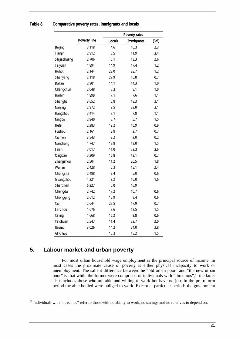
The poverty rates among permanent residents and immigrants are presented in Table 8. A notable feature is the strikingly high poverty rates in some cases: for example amongst locals in Huhot, Shenyang and Xian and amongst immigrants in Huhot, Nanjing, Jinan, Zhengzhou, Yinchuan and Urumqi. Also notable are the wide variations in the poverty rates both amongst locals and immigrants. These two features partly reflect the type of data used to derive the poverty rate. On average (the last row entitled “All Cities”, Column 3), the incidence of poverty amongst immigrants is around 50 per cent higher than amongst locals, a figure that appears plausible. One may also note that in some cities the poverty rate amongst immigrants is lower than that amongst locals. For the reasons mentioned above, this may well be the case.

19 The following five provincial capitals were excluded because of small sample: Haikou, Nanning, Guiyang, Kunming and Lhasa. 20 These five cities are termed “cities with independent planning powers”. They enjoy more extensive decision-making powers than other cities.

21

Table 8. Comparative poverty rates, immigrants and locals

Poverty rates Poverty line Locals Immigrants (3/2)

Beijing 3 118 4.6 10.3 2.3

Tianjin 2 912 3.5 11.9 3.4

Shijiazhuang 2 706 5.1 13.3 2.6

Taiyuan 1 894 14.9 17.4 1.2

Huhot 2 144 23.0 28.7 1.2

Shenyang 2 118 22.9 15.0 0.7

Dalian 2 901 14.1 14.3 1.0

Changchun 2 048 8.3 8.1 1.0

Harbin 1 899 7.1 7.6 1.1

Shanghai 3 652 5.8 18.3 3.1

Nanjing 2 972 9.5 29.0 3.1

Hangzhou 3 414 7.1 7.8 1.1

Ningbo 2 940 3.7 5.7 1.5

Hefei 2 283 12.2 10.9 0.9

Fuzhou 2 161 3.8 2.7 0.7

Xiamen 3 543 8.2 2.0 0.2

Nanchang 1 747 12.8 19.0 1.5

Jinan 3 017 11.0 39.3 3.6

Qingdao 3 209 16.8 12.1 0.7

Zhengzhou 2 504 11.2 20.5 1.8

Wuhan 2 428 6.3 15.1 2.4

Changsha 2 488 8.4 5.0 0.6

Guangzhou 4 221 9.2 15.0 1.6

Shenzhen 6 227 0.0 16.9

Chengdu 2 742 17.2 10.7 0.6

Chongqing 2 612 16.9 9.4 0.6

Xian 2 644 27.5 17.9 0.7

Lanzhou 1 676 8.6 12.5 1.5

Xining 1 668 16.2 9.8 0.6

Yinchuan 2 547 11.4 22.7 2.0

Urumqi 3 026 14.2 54.0 3.8

All Cities 10.3 15.2 1.5

5. Labour market and urban poverty

For most urban household wage employment is the principal source of income. In most cases the proximate cause of poverty is either physical incapacity to work or unemployment. The salient difference between the “old urban poor” and “the new urban poor” is that while the former were comprised of individuals with “three nos”,21 the latter also includes those who are able and willing to work but have no job. In the pre-reform period the able-bodied were obliged to work. Except at particular periods the government

21 Individuals with “three nos” refer to those with no ability to work, no savings and no relatives to depend on.

22

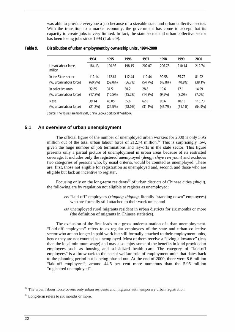
was able to provide everyone a job because of a sizeable state and urban collective sector. With the transition to a market economy, the government has come to accept that its capacity to create jobs is very limited. In fact, the state sector and urban collective sector has been losing jobs since 1994 (Table 9).

Table 9. Distribution of urban employment by ownership units, 1994-2000

1994 1995 1996 1997 1998 1999 2000

Urban labour force, million

184.13 190.93 198.15 202.07 206.78 210.14 212.74

In the State sector (%, urban labour force)

112.14 (60.9%)

112.61 (59.0%)

112.44 (56.7%)

110.44 (54.7%)

90.58 (43.8%)

85.72 (40.8%)

81.02 (38.1%

In collective units (%, urban labour force)

32.85 (17.8%)

31.5 (16.5%)

30.2 (15.2%)

28.8 (14.3%)

19.6 (9.5%)

17.1 (8.2%)

14.99 (7.0%)

Rest (%, urban labour force)

39.14 (21.3%)

46.85 (24.5%)

55.6 (28.0%)

62.8 (31.1%)

96.6 (46.7%)

107.3 (51.1%)

116.73 (54.9%)

Source: The figures are from SSB, China Labour Statistical Yearbook.

5.1 An overview of urban unemployment

The official figure of the number of unemployed urban workers for 2000 is only 5.95 million out of the total urban labour force of 212.74 million.22 This is surprisingly low, given the huge number of job terminations and lay-offs in the state sector. This figure presents only a partial picture of unemployment in urban areas because of its restricted coverage. It includes only the registered unemployed (dengji shiye ren yuan) and excludes two categories of persons who, by usual criteria, would be counted as unemployed. These are: first, those not eligible for registration as unemployed and, second, and those who are eligible but lack an incentive to register.

Focusing only on the long-term residents23 of urban districts of Chinese cities (shiqu), the following are by regulation not eligible to register as unemployed:

?? “laid-off” employees (xiagang zhigong, literally “standing down” employees) who are formally still attached to their work units; and

?? unemployed rural migrants resident in urban districts for six months or more (the definition of migrants in Chinese statistics).

The exclusion of the first leads to a gross underestimation of urban unemployment. “Laid-off employees” refers to ex-regular employees of the state and urban collective sector who are no longer in paid work but still formally attached to their employment units, hence they are not counted as unemployed. Most of them receive a “living allowance” (less than the local minimum wage) and may also enjoy some of the benefits in kind provided to employees such as housing and subsidized health care. The category of “laid-off employees” is a throwback to the social welfare role of employment units that dates back to the planning period but is being phased out. At the end of 2000, there were 8.6 million “laid-off employees”; around 44.5 per cent more numerous than the 5.95 million “registered unemployed”.

22 The urban labour force covers only urban residents and migrants with temporary urban registration. 23 Long-term refers to six months or more.

23

As is usual in any registration count, the category “registered unemployed” excludes urban residents who are unemployed but have no incentive to register. Possible reasons include not qualifying for unemployment benefit or not wanting to make use of additional benefits that come with registration such as subsidized participation in retraining programmes or job search. Such unemployed workers may include school leavers and those re-entering the labour force after a period of withdrawal because of, for example, childbirth and rearing or illness. With the shift of urban employment towards the sectors that are lightly covered by unemployment insurance (see Table 9), the percentage of the unemployed lacking an incentive to register would rise, unless counteracted by an extension of unemployment insurance.

The “registered unemployed” includes those who are in part-time or occasionally full-time informal employment. Strictly speaking these should be excluded from the headcount according to the ILO definition.24 Municipal Labour Bureaux turn a blind eye to paid employment by benefit recipients for two reasons. First, the unemployment benefit, which is not adjusted for the family circumstances of the recipients, is not sufficient to prevent a severe hardship in households with dependents. Second, casual work in the informal sector is difficult, if not impossible, to monitor with a reasonable degree of accuracy.

5.2 How high is urban unemployment?

Broadly individuals are unemployed when they are currently without a job and looking for a job. For the present purposes, “without a job” should be interpreted as a “job that provides an income at least equal to the local poverty line”, which for most manual workers means a full-time job25. Including both the “registered unemployed” and “laid-off employees” together the total number of unemployed urban workers (those without a full-time job) comes to 14.6 million. This figure suffers from errors of omissions and commissions. But this is the best that is available because it is not possible to correct for errors. What unemployment rate does the figure of 14.6 million imply? The answer depends crucially on what is taken as the relevant urban labour force (the denominator). The unemployment rate in Chinese statistics is calculated by taking as denominator the urban labour force that is not self-employed, which in 2,000 totaled around 191 million. But this figure also includes those who when unemployed are, for the most part, not counted either among “laid-off employees” or “registered unemployed”. Such workers include temporary or casual employees, the “informally employed” and private sector employees. Such workers, when unemployed, do not qualify for treatment as “laid-off employees”, and being outside the scope of unemployment insurance, nor do they have any particular incentive to register as unemployed. The implication is their inclusion increases the denominator but makes no or little difference to the numerator. Such workers excluded, the component of the urban labour force that is relevant for the calculation of the urban unemployment rate consists of “staff and workers” (the formally employed) plus the “registered unemployed”, which in 2000 totaled around 118.5 million.

Taking 14.6 million as the headcount of the unemployed, the unemployment rate comes to 12.3 per cent. Though partial and subject to errors, this figure presents a more accurate picture of unemployment (meaning without a full-time job) in urban areas than would the unemployment rate of 7.6 per cent, the rate when the denominator is taken to be 191 million (the urban labour force excluding the self-employed). Though there is no reliable estimate of unemployment in the labour force that is not included in the category

24 By the ILO definition a person is unemployed if not engaged in paid work for more than one hour per week and actively searching for a job. 25 The cut-off threshold of one hour per week is too low when the concern is the relation between unemployment and poverty.

24

“staff and workers”, there are good grounds for assuming that the unemployment rate amongst them is no less than that for “staff and workers”. Their jobs are less secure than those of “staff and workers”.

5.3 Two labour market trends and their implications

The Chinese urban labour market is undergoing two changes that have far-reaching implications for the incidence of unemployment, terms and conditions of employment and income maintenance for the unemployed. One is the changing pattern of employment and the other concerns the impact of the demographic transition on the age-composition of the labour force.

Historically, the state and the urban collective sectors (the public sector) have been the principal source of employment for the urban labour force. But since the 1990s, the sector has not only been failing to provide jobs to fresh entrants to the labour force but has also been shedding existing employees. As shown in Table 1, in seven years from 1994 to 2000, the public sector has seen its employment share plunge from 78.7 per cent to 45.1 per cent. The sector has also been losing jobs, in just four years from 1996 to 2000; state units (enterprises, public institutions and the government) have lost around 31.4 million jobs, 27.9 per cent of the total in 1996.

The trend of job losses from the public sector is expected to continue for some years because of the discharge of “laid-off employees”, who are still counted as employees, and further job losses. On the other hand, the non-public sector (comprising foreign-invested, private and household enterprises) has over the seven years from 1994 to 2000, seen its employment share jump from 21 to 54.9 per cent and its total labour force rise almost three-folds from 39 to 117 million. A shift of employment out of the public sector fits in with the transition from a planned to a market economy. But this shift raises important issues for unemployment and income maintenance of the unemployed because of the differences in the terms and conditions of employment and in social security coverage between the public and the non-public sector,

The public sector, although employs only 45 per cent of the urban labour force accounts for 83 per cent of employees classified as “staff and workers”. Most of such employees have formal labour contracts and are covered by social insurance, unemployment insurance in particular. In contrast, employees who are not classified as “staff and workers” lack formal labour contracts and have less secure jobs and are outside the umbrella of social insurance. Thus the shift of employment has accentuated the dualism in the labour market that has always existed but was previously marginal. In particular, it implies a higher unemployment rate because of more frequent job terminations and, more consequential for poverty alleviation, a substantial reduction in the percentage of unemployed entitled to unemployment benefit (including the current living allowance for “laid-off employees”). The appropriate policy response lies not in slowing down the shift of employment from the public to the non-public sector but in extending the coverage of formal employment contracts and of social insurance to the non-public sector.

6. Income maintenance for the urban poor

The urban population benefits from three lines of defence against poverty:

?? living allowance for laid-off employees;

?? unemployment insurance;

25

?? minimum living standard scheme (MLSS).

The first is the largest with around eight million beneficiaries, but it is transitory, due to be phased out by the end of 2003. Unemployment insurance is a comparatively small scheme with only 3.3 million beneficiaries. In the first nine months of year 2000, 3.2 million received the MLSS allowance.

6.1 How effective is the MLSS in reaching the urban poor?

Two crucial indicators of the effectiveness of a poverty alleviation scheme, such as the MLSS are:

?? the percentage of the identified poor who receive assistance; and

?? the likely discrepancy between the numbers of actual and identified poor.

On both counts, the MLSS currently falls short of the acceptable level. In the first nine months of 2000, while the recipients totalled 3,237,000, a survey conducted by the Ministry of Civil Affairs (MOCA) in August 2,000 put the number of urban residents with incomes below the local poverty line at 14 million. Other estimates put the number higher. According to the MOCA figure, only 23 per cent of the bona fide urban poor actually received assistance. Table 10 presents the coverage rates for three cities on the basis of a field study conducted in 2000-2001:

Table 10. % of identified poor receiving assistance

Nos. identified as poor Nos. receiving assistance (% of the identified poor)

Shenyang 130 000 38 000 (29.2%)

Xining 75 000 19 000 (25.3%)

Bengbu 40 000 10 000 (25.0%)

The above figures, although slightly higher, are in line with the MOCA survey finding that the coverage of the MLSS is very low. Local officials in charge of the scheme recognize this as a serious problem, which they attribute to a severe shortage of funds. A widespread response to the shortage of funds is to reduce the number of potential beneficiaries by tightening the qualification for receiving the MLSS assistance. A common method is to assume that all those capable of working earn a certain sum regardless of what they claim or that those entitled to a “living allowance for laid-off employees” receive the allowance even in cases where it is well known that they do not.

Apart from the low coverage of the MLSS, there is also the additional problem of the number of identified poor being lower than the actual number. For example, a recent sample survey in Bengbu revealed that the population with a per capita monthly household income of less that Y130 (the local poverty line) in the city is 80,000 (15.4 per cent of the urban population) twice as the previous estimate of only 40,000 (7.5 per cent of the urban population).26 This is perhaps an extreme case but the underestimation of the number is common because current methods of estimation rely heavily on informed guesses of local officials. A number of cities, such as Bengbu and Shenyang, have conducted sample

26 The survey was organized by the Bengbu City Civil Affairs Bureau and conducted in August and September 2000. The sample size was 10 per cent of the urban population (80,000 persons and 20,000 households).

26

surveys to identify the number of poor people in the city, but such surveys are not universal and are variable in methodology and coverage.

6.2 Problems with MLSS and possible remedies

Limited coverage

The MLSS plays a crucial role in alleviating poverty in urban areas. Being the last line of defence against urban poverty, the scheme supplements and complements social insurance and the living allowance for laid-off employees. With less than a quarter of the eligible urban poor actually receiving assistance, the MLSS is too limited in its coverage for the social safety net of the last resort. Added to this, long-term migrants (those resident in the locality for more than six months) are completely excluded. Local officials in charge of the scheme fully recognize the importance of extending the coverage of the scheme. The principal impediment to extension is the mismatch between the availability of funds and the number of the urban poor in need of assistance at the lower government tiers of urban districts municipalities. This impediment can be removed by raising the share of the cost of the scheme borne by the provincial and central governments.

Loopholes in the diagnosis of urban poverty

Last few years have witnessed an immense progress in diagnosis of urban poverty, which is the crucial first step towards its alleviation. But the diagnosis is marred by some serious weaknesses. The estimation of the number of poor at the local level still relies heavily on informed guess. Some cities have undertaken special surveys to identify the incidence of poverty but such surveys are still sporadic and variable in methodology and coverage.

Local governments set poverty lines for estimating the headcount of the poor and for determining assistance. This is how it should be. China is a populous country and covers an extensive area. Patterns of consumption, prices and the average per capita income (or the living standard) vary widely across provinces and between cities in the same province. In principle, local poverty lines are determined by costing the goods and services for basic subsistence. But the city governments that set the poverty lines are also responsible for financing the MLSS. As a result, fiscal considerations enter in the determination of local poverty lines. The general consensus is that poorer cities are forced by their strained public finances to set poverty lines that are too low to ensure basic subsistence.

There are strong arguments for differentiating between the poverty line for diagnosis and the poverty line for determining assistance. The former could be used to assess the effectiveness of current poverty alleviation and set a target for the future. There are a number of national organizations, such as the NSB, which calculate poverty line purely for the purpose of estimating the headcount of the poor population. These poverty lines serve as a useful benchmark, but their value is limited by the fact that they do not allow for regional variation in prices and consumption pattern.

What is needed are the following:

?? standardized statistical surveys aimed at the estimation of poverty;

?? a detailed national framework for the calculation of poverty lines by city governments; and

?? calculation of diagnostic poverty lines not merely for the whole of China but also for provinces and regions within a province.

27

Insufficient benefits

The MLSS restricts itself to just making up the difference between household income per capita and the poverty line. Unlike in some countries, assistance is not adjusted to take account of the number of household members (scale effect) and their ages. This is justified because the MLSS is in its initial stages of development and its administration is already a heavy burden on the local government.

The actual MLSS benefit per person is low. Over nine months from January to September 2000, the average cash benefit amounted to Y75 per month/person. This poses a problem because of two factors. First, household per capita income is frequently calculated on the basis of “presumptive income” rather than actual income so as to keep within the limited budget. Second, the poverty line that sets the threshold for assistance is in many localities too low. In principle, these problems can be handled through national guidelines for estimating actual incomes and for calculating the poverty line for the purpose of providing assistance.

But MLSS assistance to poor urban households suffers from two major gaps that limit its effectiveness as the social safety net of last resort.

First, unlike unemployment insurance, the MLSS provides no healthcare insurance, not even against serious illness. The poverty line is supposed to include an allowance for healthcare expenditure. But that allowance is purely notional and not adjusted for recipients’ state of health. There is ample evidence that MLSS recipients, many of whom suffer from chronic illnesses, and other low-income urban households forego necessary medical care and avoid visit to doctors and hospitals. There are strong arguments in favour of a means-tested free healthcare insurance covering serious illnesses for the urban population as a central component of poverty alleviation.

Second, the cost of schooling has risen sharply in recent years and constitutes a heavy burden for low-income urban households with children. They face a difficult choice between providing proper education to their children at the cost of cutting down an already low expenditure on daily necessities, on the one hand, or cutting down on education expenditure. There are strong arguments in favour of the establishment of an education fund to assist low-income households with the schooling cost of their children.

Poverty alleviation and maintaining incentive to work

The central issue confronting social welfare in market economies is how to protect those capable of working through poverty, while maintaining incentive to work on their part. In the past this issue was addressed by providing them with a job, an option that is no longer feasible. The issue is currently not in the forefront because of a sharp rise in the number of unemployed and laid-off workers, on the one hand, and the apparent scarcity of jobs. Both the MLSS and the unemployment insurance scheme will have to address this issue by instituting procedures and programmes to oblige and encourage those capable of working to raise themselves out of poverty though wage or self-employment.

There are a wide variety of initiatives on the part of the local government and non-governmental organizations, such as the Labour Union and Women’s Association, to help the unemployed and laid-off employees to find jobs or start their own businesses. However, there is a need for schemes linked to the MLSS that are aimed at job creation and setting-up own businesses.

Financing

The total expenditure on the MLSS at the national level is extremely low. In 1998 it amounted to a mere 0.15 per cent of the consolidated government expenditure. Raising the

28

coverage rate of the scheme (the percentage of the poor receiving assistance) four fold to 100 per cent would still keep the total cost of the MLSS well below 1 per cent of the total government expenditure, at 0.6 per cent.

Yet the scheme is severely constrained by a shortage of funds. The reason is not the total cost but its distribution across government tiers. Despite cost sharing by higher government tiers, city districts (the lowest but one government tier) end up bearing a high share of the cost of the scheme. City districts are too small a unit to spread the cost of supporting the urban poor equitably. The incidence of poverty across city districts is highly uneven. Added to that, districts with a higher percentage of the poor also tend to have more strained public finances.

In general, the current arrangement for financing the MLSS is makeshift. As it currently stands it is neither equitable nor does it yield sufficient funds relative to obligations. What is needed is a re-allocation of costs towards higher government tiers of the centre and provinces and a corresponding reduction of the cost by lower government tiers.

Administrative structure

Though it currently reaches no more than a quarter of the bona fide urban poor, the MLSS is a large social security scheme with 3.25 million beneficiaries in the first nine months of 2000. The urban population with an income lower than the local poverty line, according to a survey by MOCA, is 14 million. For its day-by-day operation, the scheme still relies on a handful of officials at the level of municipalities, urban districts and street offices. In terms of the number of officials and material resources, the administrative structure falls well short of what is needed for an effective operation of the scheme. The present administrative infrastructure of the MLSS is carried over from the past when urban poverty relief was confined to persons with “three nos”. As a result, there is a gross mismatch between the aim of assisting all the urban residents with an income below the local poverty lines and the administrative structure of the scheme.

7. Conclusion

A large majority of poor in China are rural inhabitants, mostly from remote mountainous areas. However, urban poverty that until the mid-1990s was regarded as a minor affliction confined to a small minority has since emerged as a major social issue and seen as a threat to social stability. This is due in part to a change in the social perception of poverty. Against the background of an average living standard that is historically high and rising, what previously would have been regarded as a low living standard now appears as deprivation. The “new urban poverty” is in large measure due to a change in the urban economic environment. The state sector and urban collective enterprises that have traditionally been the sources of employment for the urban labour force have been losing jobs, a trend that is expected to continue apace for some years. The non-state sector has grown but not rapidly enough to absorb both surplus rural labour and redundant urban labour.

How many urban poor are there and what is the urban poverty rate? Unlike in the recent past, it is now possible to answer these questions precisely, if not accurately. The Ministry of Civil Affairs (MOCA) puts the number of urban poor at 14 million. This estimate answers one question but raises a number of questions that cast doubt on its reliability. Of these the following two are crucial:

29

??What is the definition of the urban population?

??What is the poverty line?

The definition of “urban” in China departs in some crucial respects from the usual definition of urban. The definition matters because the urban poverty line can be between two to three times that of the rural poverty line. A person can be non-poor by the rural poverty line but poor in terms of the urban poverty line. In terms of the usual socio-economic criteria of population density and sources of livelihood, the percentage of the urban population in China is substantially higher than the official 36 per cent. A reclassification of the Chinese population into urban and rural in line with the usual criteria would raise the urban poverty rate for China by a wide margin. In particular, the inclusion of millions of rural immigrants living and working in cities in the urban population would have a substantial impact on the poverty rates for major Chinese cities.

A major contribution of this paper is that it bases its analysis of urban poverty on provincial poverty lines calculated according to best international practice from the NSB urban household data for whole China. The data set suffers from shortcomings but it provides by far the most comprehensive coverage of the urban population. The paper pays special attention to methodological issues that arise in the calculation of poverty line, including the following:

?? geographical coverage of the line;

?? the difference that the choice of income or expenditure makes to the headcount of the poor;

?? adjustment for household size;

?? the sensitivity of the poverty rates to shifts in the poverty line.

The salient features of the urban poverty profile presented in the paper are the following:

?? given the wide variation in provincial poverty line, the use of a single poverty line for whole China will present a very distorted picture of urban poverty, exaggerating the poverty rate in the interior provinces and under-stating the rates in the coastal provinces;

?? it makes a huge difference whether poverty is identified in terms of income or expenditure per head. Focusing on household income per head, the average urban poverty rate for China is very low (4.73 per cent) by the standards of developing economies. However, the provincial rates vary widely;

?? the national headcount of the poor shoots up by just over 2.5 times, from 14.7 million to 37.1 million, if the poor are identified in terms of expenditure per head instead of income per head. The reason is not so much that low income households in China save a lot but that in terms of income per head they are densely clustered around the poverty line such that even a small amount of savings is sufficient to push them below the poverty line in terms of expenditure per head;

?? the poverty headcount and rate are highly sensitive to slight shifts in the poverty line. An increase in the national poverty line by 15 per cent raises the national poverty rate by as much as 72.7 per cent from 4.7 to 8.2 per cent of the urban population. Raising the poverty line by another 10 percent raises the national poverty rate by 43.2 per cent from 8.2 to 11.1 per cent of the urban population. The latter poverty rate is close to the poverty rate when expenditure instead of income per head is used as the indicator. This indicates

30

that in terms of impact on the national poverty rate, the change in the indicator from income to expenditure is equivalent to raising the poverty line by just over 25 per cent, while keeping income per head as the indicator of poverty.

The salient implications of the acute sensitivity of the poverty rate to a comparatively small shift in the poverty line, which also happens to be true of the rural poverty profile, is that a significant percentage of the non-poor urban population remains highly susceptible to a fall into poverty as a result of a relatively small reduction in income or, for example, a rise in non-food expenditure as a result of illness. This suggests that the focus of poverty alleviation measures should not be confined to those who fall below the poverty line, it should also extend to the population with a high risk of falling into poverty. The appropriate policy response with respect to the latter group is not social assistance but increasing the capability of low-income households to cope with risks, by, for example, provision of health insurance against serious illness. The vulnerability of a substantial percentage of the urban population falling into poverty as a result to comparatively small decrease in household income per head also emphasises the importance of a social safety net that covers all urban population rather than, as in the past and still so in practice, a small section of the population with no ability to work, no savings and no relatives to depend on.

31

References

Atkinson, A. B. 1998. Poverty in Europe (Blackwell).

Deaton, A. 1997. The Analysis of Household Surveys: A Microeconometric Approach (Baltimore, The Johns Hopkins University Press for the World Bank).

Ravallion, M. 1994. Poverty Comparisons (Switzerland, Harwood Academic Publishers).

________. 1998. Poverty Lines in Theory and Practice (World Bank), LSMS Working Paper No. 133.

Sen, A.K. 1983. “Poor Relatively Speaking”, in Oxford Economic Papers, Vol. 35.

________. 1992. Inequality Reexamined (Oxford University Press).

33

Other papers in the SES Series

?? Worker Insecurities in Ukrainian Industry: The 1999 ULFS by Guy Standing and László Zsoldos, InFocus Programme on Socio-Economic Security.

?? Globalisation and Flexibility: Dancing Around Pensions by Guy Standing, InFocus Programme on Socio-Economic Security.

?? Unemployment Benefits and Income Security by Guy Standing, InFocus Programme on Socio-Economic Security.

?? Modes of Control: A Labour-Status Approach to Decent Work by Guy Standing, InFocus Programme on Socio-Economic Security.

?? Workfare Tendencies in Scandinavian Welfare Policies by Nanna Kildal, Centre for Social Research, University of Bergen, Norway.

?? Combining Compensatory and Redistributive Benefits: The Challenge of Social Policies in Brazil by Lena Lavinas, InFocus Programme on Socio-Economic Security.

?? The Appeal of Minimum Income Programmes in Latin America by Lena Lavinas, InFocus Programme on Socio-Economic Security.

?? Socio-Economic Security, Justice and the Psychology of Social Relationships by Rosamund Stock, Department of Social Psychology, London School of Economics.

?? Socio-Economic Security in the Context of Pervasive Poverty: A Case Study of India by Seeta Prabhu, Human Development Resource Centre, UNDP, New Delhi.

?? Employment Security: Conceptual and Statistical Issues by Sukti Dasgupta, InFocus Programme on Socio-Economic Security.

?? Worker Insecurities in the Ukrainian Industry: The 2000 ULFS by Guy Standing and László Zsoldos, InFocus Programme on Socio-Economic Security.

?? Does Informal Credit Provide Security? Rural Banking Policy in India by V.K. Ramachandran and Madhura Swaminathan, Indian Statistical Institute, Calcutta

?? Workfare Programmes in Brazil: An Evaluation of Their Performance by Sonia Rocha, Institute for Applied Economic Research, Brazil.

?? Applying Minimum Income Programmes in Brazil: Two Case Studies by Sonia Rocha, Institute for Applied Economic Research, Brazil.

?? Assessing Local Minimum Income Programmes in Brazil by Lena Lavinas, InFocus Programme on Socio-Economic Security; Octavio Tourinho and Maria Lígia Barbosa, ILO Area Office in Brazil.

?? Changing Employment Patterns and the Informalization of Jobs: General Trends and Gender Dimensions by Lourdes Beneria, Cornell University.

?? Coping with Insecurity: The Ukrainian People’s Security Survey by Guy Standing and László Zsoldos, InFocus Programme on Socio-Economic Security.

?? Social Protection for Informal Workers: Insecurities, Instruments and Institutional Mechanisms by Jeemol Unni and Uma Rani, Gujarat Institute for Development Research, Gota, India.

?? Sustainable Development of the Global Economy: A Trade Union Perspective by Winston Gereluk, Public Services International and Lucien Royer, Trade Union Advisory Committee to the OECD.

34

?? Employment Security in Europe and Canada: A Review of Recent Legislation in Three Countries by Walter Onubogu, InFocus Programme on Socio-Economic Security.

?? Innovations in Monitoring Work Security: A Case Study of Southeast Asian Refugees in Lowell, Massachusetts by Lenore Azaroff and Charles Levenstein, Department of Work Environment, University of Lowell, Massachusetts.

?? Health Care in Central and Eastern Europe: Reform, Privatization and Employment in Four Countries – A Draft Report for the International Labour Office InFocus Programme on Socio-Economic Security and Public Services International.

?? Failing Health Systems: Failing Health Workers in Eastern Europe by Carl Warren Afford, InFocus Programme on Socio-Economic Security (also available in Russian).

?? Socio-Economic Status of Health Care Workers in the Russian Federation by Natalia Stepantchikova, Liana Lakunina and Tatyana Tchetvernina, Centre for Labour Market Studies, Institute of Economics, Russian Academy of Sciences (also available in Russian).

?? Exclusion, Précarité, Insécurité Socio-Économique (Apports et débats des sciences sociales en France) and La Prise en Compte de l'Insécurité Socio-Économique dans les Grandes Enquêtes Statistiques en France by Helena Hirata, Groupe d’Etudes sur les Rapports Sociaux de Sexe and Edmond Préteceille, Centre de Sociologie Urbaine, Institut de Recherche sur les Sociétés Contemporaines, Centre National de la Recherche Scientifique.

?? Is there a Welfare State Crisis? A Comparative Study of French Social Policy by Robert Boyer, Centre d’Etudes Prospectives d’Economie Mathématiques Appliquées à la Planification, Paris.

?? Social Policy with Respect to Care: A Perspective for Sub-Saharan Africa by Kanyhama Dixon-Fyle, Independent Consultant.

?? Workers’ Representation Insecurity in Brazil: Global Forces, Local Stress by Adalberto Moreira Cardosa, Instituto Universitário de Pesquisas do Rio de Janeiro, Brazil.

?? An Evaluation Methodology for Minimum Income Programmes in Brazil by João Saboia, Federal University of Rio de Janeiro and Sonia Rocha, State University of Rio de Janeiro.

?? Insecurities of Informal Workers in Gujarat, India by Jeemol Unni and Uma Rani, Gujarat Institute for Development Research, Gota, India.

?? Organizing for Socio-Economic Security in India by Sukti Dasgupta, InFocus Programme on Socio-Economic Security.

?? Income (In)Security in Argentina by Alberto C. Barbeito and Ruben M. Lo Vuolo, Centro Interdisciplinario para el Estudio de Politicas Públicas (CIEPP), Buenos Aires, Argentina.

?? The Institutionalization of Unemployment in Urban China: Processes, Policies and Implications by Edward Gu, East Asian Institute, National University of Singapore.

Statistical and Methodology Series:

Concealed Unemployment in Ukrainian Industry: A Statistical Analysis by Maria Jeria Caceres, InFocus Programme on Socio-Economic Security.