urban poverty in vietnam: determinants and policy implications · 2019-09-27 · vu hoang linh...

Munich Personal RePEc Archive

Urban Poverty in Vietnam:

Determinants and Policy Implications

Nguyen Viet, Cuong and Vu Hoang, Linh and Nguyen,

Thang

10 December 2010

Online at https://mpra.ub.uni-muenchen.de/40767/

MPRA Paper No. 40767, posted 20 Aug 2012 23:25 UTC

1

Urban Poverty in Vietnam:

Determinants and Policy Implications

Nguyen Viet Cuong

Vu Hoang Linh

Nguyen Thang1

Abstract2

This study examines the profile and determinants of poverty in the two largest cities in

Vietnam – Hanoi and Ho Chi Minh. Data used in this study are from the 2009 Urban

Poverty Survey. Using the poverty line of 12,000 thousand VND/year, the poverty

incidence is estimated at 17.4 percent for Hanoi and 12.5 percent for Ho Chi Minh (HCM)

city. There is a large proportion of the poor who are found stochastically poor. Hanoi has

higher rates of structurally poverty than HCM city. The proportion of structurally poor and

stochastically non-poor is rather small. Overall, the poor have fewer assets than the non-

poor. The poor also have poorer housing conditions, especially they have much lower

access to tap water than the non-poor. Heads of the poor households tend to have lower

education and unskilled works than the heads of the non-poor households.

Keywords: Urban poverty, income, expenditure, household survey, Vietnam.

1 Nguyen Viet Cuong and Vu Hoang Linh from Indochina Research & Consulting (IRC); Nguyen Thang from the Center for Analysis and Forecast, Vietnam. Contact email: [email protected]; [email protected] ; and [email protected] 2 This study is carried out with financial supports from the United Nations Development Programme in Vietnam. We would like to thank Nguyen Tien Phong, Nguyen Bui Linh, and Alex Warren-Rodriguez from UNDP, Tran Ngo Thi Minh Tam from Center for Analysis and Forecast, Vietnam for their help and comments.

2

1. Introduction

Vietnam is an example of a country where broad-shared economic growth has been

prevailing in the 1990s and 2000s. Economic reforms initiated in the late 1980s

significantly changed the economy of Vietnam, from severe stagnation in the 1980s to

high growth with an average annual rate of Gross Domestic Product (GDP) per capita of

around 7 percent during the past two decades. The fact that Vietnam has committed itself

to follow the “growth with equity” strategy as a principle to the development path

suggests that high economic growth would result in remarkable reduction in poverty.

According to Vietnam Living Standard Surveys (VHLSS), the proportion of the poor to

the population decreased from 58 percent to 14 percent between 1993 and 2008.

However, the pace of poverty reduction appears to have slowed down recently,

especially in urban areas. There are some challenges to further reduction of poverty in

Vietnam. Firstly, when poverty rate is as low as it is now, a relatively large proportion of

the poor are in chronic poverty, which tend to be more resistant to economic growth. In

other words, growth elasticity of poverty reduction in Vietnam tends to decrease

Secondly, economic growth itself has slowed down since 2008 due to the global economic

crisis. As economic growth has been the main driver of poverty reduction in Vietnam

(Dollar and Kraay, 2000), lower rate of economic growth may result in even slower

poverty reduction. Thirdly, the proportion of households who are just above the poverty

line tends to increase, indicating that a growing number of near-poor households are

vulnerable to shocks (economic and social) and that protecting the near poor from falling

back into poverty is becoming increasingly important for sustaining poverty reduction in

Vietnam in the context of the country intensifying her integration into the world economy

whereby the economy tends to grow faster but less safely. Fourthly, the integration

process also produces the so called agglomeration effects with the resultant acceleration of

the urbanization process. There are at least two consequences of this process. (i) urban

poverty and urban inequality are becoming a considerably bigger policy issue; and (ii) the

urban growth impacts overall poverty both directly - through reducing urban poverty and

indirectly - through raising earnings of low income migrant workers and thereby reducing

rural poverty. In other words, reducing overall poverty requires that in urban areas, policy

3

should give due attention not only to the urban poor, but also to the urban low income,

who tend to strengthen the rural-urban linkages in Vietnam’s development. Furthermore,

in the context of Vietnam becoming a lower middle income country, the problem of urban

poverty is becoming increasingly complex, with the need to properly take into account

various non-income aspects of people’s well-being. This further justifies the need to

include the low income in this study, as income/expenditure based poverty rates may

underestimate urban poverty, as non-income dimensions including pollution, personal

safety, working and housing conditions, exposures to abuses are becoming increasingly

acute for low income migrants who are technically classified as non-poor by income or

expenditure measures. They therefore deserve adequate attention in policy design.

With a view to providing information on the above mentioned emerging issues,

this study examines the current profile of the urban poor and the urban low income,

especially in Hanoi and Ho Chi Minh cities in Vietnam, and some key structural

relationships linking their poverty/income status with their characteristics and policy

variables and on this basis proposes policy implications for urban poverty. Although there

are a large number of studies on poverty in Vietnam, research evidence on urban poverty

is quite scarce. Perhaps the most detailed study of urban poverty is Oxfarm and ActionAid

Vietnam (2008), which provides qualitative assessment of poverty. However, this study is

based on a participatory approach without representative surveys. It is not possible

extrapolate this study’s findings beyond sites where the surveys were carried out.

There might be at least two reasons for limited research on urban poverty. Firstly,

poverty remains largely a rural phenomenon in Vietnam, hence most poverty-related

studies have up to now focused on rural poverty rather than urban poverty. Secondly,

household surveys which are used for poverty analysis often have small sample sizes,

which does not allow to do any reliable study on urban poverty in Vietnam. VHLSSs are

representative for the whole urban population, but not for the urban poor population,

because of too small number of observations on the latter. In this context, the Urban

Poverty Survey in 2009 with a relatively large sample size can fill in this data gap and will

hopefully allow for a reliable measurement and quantitative assessment of urban poverty

in Hanoi and Ho Chi Minh cities.

4

Assessment of urban poverty is of interest to researchers as well as policy makers,

particularly because it can potentially provide helpful information for devising poverty

reduction policies in the largest cities Hanoi and Ho Chi Minh in particular and in the

urban areas in general. Urban poverty and rural poverty can differ in several aspects.

Firstly, urban poverty did not experienced reduction during 2000s. According to VHLSSs,

the poverty rate was almost unchanged, at nearly 4 percent, during the period 2002-2006.

It means that urban poverty is mainly chronic or urban people are more vulnerable to

poverty. Secondly, urban poverty can be underestimated using household surveys. People

who are sampled in household surveys such as VHLSSs are often from the registered

population. Migrants and unregistered people in urban areas who are more likely to be

poor are not sampled in household surveys. Thirdly, the urban poor can include a large

number of temporary migrants and unregistered people. These groups are more vulnerable

to economic shocks and not entitled for social protection policies such as credit subsidy

and health insurance. Temporary/circular migration from rural to urban areas makes the

urban poverty more complicated, and it is more difficult to devise policies to reduce urban

poverty. Fourthly, there is a widening gap in welfare even within urban areas.

The main objectives of this study are to examine characteristics of the poor and to

investigate determinants of poverty in urban Vietnam, and the recently emerging issue of

rising inequality within urban areas. The paper is structured into 6 sections. Section 2

analyzes the main characteristics of the urban poor. Section 3 examines factors

determining poverty, income and consumption expenditure in Hanoi and HCM city.

Section 4 presents the analysis of dynamic poverty. Income inequality is analyzed in

section 5. Finally, section 6 concludes.

2. Urban poverty and characteristics of the poor

2.1. Data set

5

This study relies mainly on data the Urban Poverty Survey (UPS) which was conducted by

the Hanoi Statistics Office and the Ho Chi Minh City (HCMC) Statistics Office in October

2009. This sample of households and individual persons is representative for Hanoi and

HCMC. The main objectives of the UPS are to assess urban poverty in Hanoi and HCMC.

It is very interesting that the survey contains information on the migrants and unregistered

households and the non-household based population. Data from this survey are quite

detailed, including income, consumption, employment, education, health care, risks and so

on. The number of observations of the 2009 UPS is 1,637 and 1,712 for Hanoi and Ho Chi

Minh city, respectively.

Although not comparable, it is still useful to see how similar/different the urban

profile provided by VHLSS 2008 is from a “zoom-in” urban picture by the UPS 2009. In

addition, we can also compare the data from the 2009 Population Census and Houseing.

This quick look reveals, as shown in Table 1 that the proportion of households having

assets tends to be lower in the 2009 UPS than in the 2008 VHLSS. Possibly, the UPS

2009 covered a larger proportion of migrants than the 2008 VHLSS. However, three data

sources give relatively similar estimates.

Table 1: Comparison of variables between VHLSS 2008 and UPS 2009

VHLSS 2008 Population Census 2009 UPS 2009

All Urban Rural All Urban Rural All Urban Rural

% household living in

urban areas 78.3 100.0 0.0 62.8 100.0 0.0 74.3 100.0 0.0

Household demography

% with male head 59.5 57.5 67.0 63.1 57.3 72.8 60.8 58.1 68.8

Age of head 51.6 52.4 48.9 45.0 44.9 45.1 46.7 47.0 45.7

% household members above 60

11.8 12.8 8.5 9.4 8.4 11.1 9.6 9.8 9.1

% household members below 15

19.3 18.7 21.6 18.5 17.2 20.6 20.5 20.0 21.8

% female members 52.3 52.6 51.2 52.3 52.6 51.8 52.9 53.0 52.6

Household size 4.2 4.1 4.3 3.7 3.7 3.7 3.8 3.7 4.0

% households with assets

Motorbike 90.1 90.8 87.7 85.3 90.3 76.8 88.7 90.3 84.3

Television 98.0 98.3 96.8 92.0 92.7 90.8 95.2 95.3 95.0

Computer 37.9 43.2 19.0 35.8 48.2 15.0 44.0 50.2 25.7

Fridge 79.6 84.2 62.9 59.9 71.0 41.2 75.0 79.6 61.6

Mobile phone 74.8 80.4 54.6 n.a. n.a. n.a. 90.5 92.7 84.2

Desk telephone 75.9 76.6 73.2 59.9 66.3 49.0 67.5 70.1 59.8

Internet connection 23.7 28.6 6.2 n.a. n.a. n.a. 30.5 36.4 13.6

Housing

Living areas per capita (m2) 22.1 22.0 22.5 30.9 34.6 24.5 22.3 23.3 19.4

6

VHLSS 2008 Population Census 2009 UPS 2009

All Urban Rural All Urban Rural All Urban Rural

% housing with tap water 64.5 78.2 14.8 48.3 71.5 9.0 61.1 75.4 19.5

% housing with flush toilet 92.5 96.3 78.6 69.7 90.9 34.0 91.0 97.4 72.5

Education degree of head

No degree 17.6 16.2 22.8 2.1 1.8 2.6 11.6 9.7 17.2

Primary 20.2 16.2 34.5 16.6 14.1 20.6 17.8 16.6 21.2

Lower secondary 20.0 19.6 21.3 32.4 25.5 44.0 27.5 25.1 34.7

Upper secondary 16.0 18.0 8.7 31.6 35.4 25.3 24.0 24.9 21.2

Post secondary 26.2 30.0 12.7 17.4 23.2 7.4 19.0 23.6 5.7

Occupation of head

Manager 3.0 3.0 2.9 n.a. n.a. n.a. 4.2 5.1 1.5

Technician 11.4 14.0 1.8 n.a. n.a. n.a. 15.8 19.1 6.2

Service, clerk, office 7.9 9.1 3.7 n.a. n.a. n.a. 19.8 21.0 16.2

Skilled worker 8.5 1.8 32.8 n.a. n.a. n.a. 13.1 10.6 20.6

Machine users 15.4 15.2 16.2 n.a. n.a. n.a. 10.1 10.5 8.9

Unskilled & Farmers 20.6 20.6 20.9 n.a. n.a. n.a. 13.3 9.1 25.4

Not working 33.2 36.4 21.6 n.a. n.a. n.a. 23.7 24.6 21.2

Income & expenditure

(thousand VND in 2009

price)

Per capita income 25713 28518 15610 n.a. n.a. n.a. 30368 34077 19627

Per capita expenditure 22108 24722 12693 n.a. n.a. n.a. 24723 27982 15284

Number of poor households (Obs.)

540 426 114 326226 195102 131124 1748 1155 593

Source: Authors’ estimation from the 2009 UPS.

2.2. Urban poverty and characteristics of the poor

Poverty line

Key poverty indicators estimated on the basis of various poverty lines are reported in

Table 2. The poverty line used in the paper as the base case is the official poverty line of

Ho Chi Minh City, which is set at 12,000 thousand VND per capita per year (Decision No.

23/2010/QDUB issued by Hanoi People’s Committee on 29/3/2010 on the poverty line for

Ho Chi Minh city during the period 2009-2015). The official poverty line which is set by

Hanoi People’s Committee is 6,000 and 3,960 thousand for urban and rural areas,

respectively (Decision No. 1592/QDUB issued by Hanoi People’s Committee on 7/4/2009

on the poverty line for Hanoi during the period 2009-2013). Using this Hanoi poverty line,

the poverty rate is only 1.6 percent in Hanoi. There are only 36 poor households in the

7

sample of Hanoi, which is too small for any meaningful quantitative analysis. Beside this

technical problem, the deprivations and hardships of the urban poor, as mentioned earlier,

tend to be underestimated if income or expenditure is used to measure the well-being of

the urban dwellers. Using the poverty line of 12,000 thousand VND, the poverty incidence

is estimated at 17.4 percent for Hanoi and 12.5 percent for HCM city. Table 2 shows also

shows the poverty rate using different income poverty. The national poverty line was set

by the government in 2006, which is equal to 200 and 260 thousand VND/person/month

for rural and urban areas, respectively. Using the price deflator, these poverty lines are

equal to 3701 and 4778 thousand VND/person/year, respectively. The income poverty

lines of 1.25$ and 2$ PPP/day are also used.3 The table shows that a better performance of

HCM City over Hanoi in every poverty indicator (except the poverty line of City People

Committee), which is also robust across different poverty lines. This difference is

acceptable, as Hanoi and Ho Chi Minh City are the richest urban centers, presumably

considerably outperforming the remaining cities in Viet Nam.

Table 2: Key poverty indicators by different poverty lines

City

National income

poverty line

Income poverty line of People

Committee

Income poverty line of HCM city

Income poverty line

1.25$ PPP/day

Income poverty line 2$ PPP/day

Poverty line/person/year (thousand VND)

4778 for urban; 3701

for rural

6000, 3960 Hanoi, 12000

HCM

12000 4135 6612

Poverty rate (%)

Hanoi 1.27 1.56 17.38 1.34 4.57

HCM city 0.31 12.52 12.52 0.29 2.08

Total 0.65 8.71 14.21 0.65 2.95

Poverty gap index

Hanoi 0.0040 0.0052 0.0531 0.0046 0.0127

HCM city 0.0008 0.0321 0.0321 0.0007 0.0034

Total 0.0019 0.0228 0.0394 0.0021 0.0066

Poverty severity index

Hanoi 0.0018 0.0023 0.0244 0.0021 0.0059

HCM city 0.0004 0.0116 0.0116 0.0003 0.0012

Total 0.0009 0.0084 0.0161 0.0009 0.0028


3 Tháng 9/2010, Chính ph� v�a ban hành chu�n nghèo m�i áp d�ng cho giai �o�n 2011-2015 là khu v�c thành th: 500.000 �ng/ngư�i/tháng và nông thôn: 400.000 �ng/ngư�i/tháng

8

Characteristics of the poor

Table 3 presents the basic characteristics of the poor defined by different poverty lines.

Overall, the very poor households are those who have only one or two members with a

female and young head. Poor heads are more likely to have low level of education

attainment and unskilled/low skilled jobs. The very poor households tend to be migrants in

urban areas and live in a dormitory or houses of poor conditions.

Overall the non-poor have more assets than the poor. The proportion of the non-

poor having computer, internet connection, and fridge is much higher than the poor. The

proportion of households owning a computer is very low for the poor.

Heads of the poor households tend to have lower education and unskilled works

than the heads of the non-poor households. For the national poverty line, there are only 0.7

percent of heads in poor households obtaining a post-secondary degree, while 17.1 percent

of heads in non-poor households have a post-secondary degree. These findings are also

similar to findings from ActionAid (2009).

Households who do not have a registration book (called ho khau), and those who

have arrived Hanoi and Ho Chi Minh cities since 2008 are more likely to be poor. The

poor have poorer housing conditions, especially they have much lower access to tap water

and flush toilet than the non-poor. The poor tend to live in a house without concrete roof.

Regarding to employment, the poor are more likely to work for households as unskilled

workers. As the poverty line increases, the gap in welfare indicators between the poor and

non-poor is reduced.

Table 3 also presents the income and expenditure patterns of the poor in Hanoi and

HCM city. The poor have much lower income and consumption than the non-poor.

However, the pattern of income as well as consumption is very similar between the poor

and non-poor.

9

Table 3: Characteristics of poor and non-poor in Hanoi and HCM city

Variable

National income poverty line

Income poverty line of People Committee


Income poverty line 1.25$ PPP/day


Poor Non-Poor Poor Non-Poor Poor Non-Poor Poor Non-Poor Poor Non-Poor

% household living in urban areas 62.93 76.50 68.83 77.08 54.52 79.80 54.42 76.57 55.57 77.08

Without registration book 65.90 29.60 34.76 29.50 29.03 30.10 62.43 29.65 40.45 29.60

% household members above 60 7.21 8.06 10.79 7.79 10.76 7.62 8.38 8.04 11.36 7.93

% household members below 15 10.26 16.23 18.69 15.93 20.16 15.54 11.64 16.21 18.20 16.10

% female members 55.73 53.34 51.83 53.51 54.53 53.18 56.07 53.34 57.36 53.22

Household size 2.10 3.21 3.24 3.20 3.35 3.18 2.28 3.21 2.85 3.21


Motorbike 14.43 76.38 55.60 77.67 56.76 78.76 14.88 76.34 38.16 77.06

Television 23.22 79.82 67.57 80.36 70.16 80.69 26.89 79.75 50.40 80.25

Computer 0.00 36.51 11.54 38.47 10.99 40.10 0.00 36.48 6.48 37.17

Fridge 0.00 60.70 35.55 62.42 36.67 63.79 0.00 60.66 21.72 61.42

Mobile phone 32.67 87.06 66.73 88.39 66.22 89.71 31.03 87.04 50.55 87.75

Desk telephone 1.76 54.30 32.36 55.80 39.20 56.08 1.88 54.27 26.71 54.71

Internet connection 0.00 24.96 4.10 26.65 4.36 27.91 0.00 24.94 0.00 25.56

Housing

Ling in dormitory 28.87 17.37 20.03 17.24 13.70 18.08 27.47 17.39 19.07 17.43

Living areas per capita (m2) 12.26 22.27 21.94 22.19 18.47 22.75 12.78 22.26 14.08 22.45

% housing with concrete roof 21.73 42.06 14.72 44.42 37.04 42.62 26.14 42.01 33.63 42.15

% housing with concrete floor 71.19 89.97 84.82 90.26 82.93 90.87 73.00 89.95 75.97 90.26

% housing with tap water 29.06 56.36 42.17 57.40 35.69 59.30 23.29 56.40 29.51 57.00

% housing with flush toilet 48.09 88.73 79.38 89.17 71.35 91.00 47.70 88.70 59.30 89.32

% households using gas and electricity for cooking

30.83 82.57 67.29 83.46 60.44 85.46 30.00 82.55 47.90 83.24

Characteristics of household head

% head single 46.10 20.02 27.09 19.63 20.86 20.18 39.45 20.09 34.30 19.79

% with male head 52.99 57.49 53.85 57.79 55.06 57.83 54.59 57.48 55.75 57.51

Age of head 36.25 42.91 43.37 42.79 44.16 42.63 38.97 42.88 41.04 42.90

Head has been arrived since 2008 63.74 16.37 28.55 15.73 24.62 15.61 59.23 16.44 39.09 16.07


No degree 27.76 10.95 28.26 9.50 24.00 9.09 29.69 10.94 26.73 10.58

10

Variable







Primary 25.75 18.93 31.96 17.78 26.37 17.84 23.42 18.96 21.73 18.91

Lower secondary 29.69 29.09 24.61 29.52 31.33 28.74 25.52 29.13 34.62 28.90

Upper secondary 16.13 23.96 14.62 24.76 16.39 25.06 20.65 23.91 16.61 24.13

Post secondary 0.67 17.07 0.55 18.45 1.91 19.27 0.72 17.06 0.31 17.48

Occupation of head

Manager 0.00 3.39 1.51 3.54 1.05 3.73 0.00 3.39 3.93 3.34

Technician 0.00 14.80 0.79 15.97 1.58 16.72 2.99 14.77 0.94 15.13

Service, clerk, office 10.05 18.73 15.24 18.97 12.89 19.55 9.68 18.73 9.06 18.97

Skilled worker 7.72 14.96 16.80 14.71 18.19 14.37 7.73 14.96 13.22 14.95

Machine users 5.30 11.98 9.50 12.15 6.97 12.70 3.85 11.99 7.37 12.07

Unskilled & Farmers 61.48 17.23 27.62 16.73 34.30 15.05 57.21 17.30 44.10 16.76

Not working 15.46 18.89 28.54 17.94 25.03 17.88 18.53 18.86 21.37 18.77

Head's employers

State 1.35 13.37 1.33 14.38 3.43 14.80 0.86 13.37 1.88 13.64

Private 15.78 19.62 17.64 19.76 15.25 20.26 18.06 19.59 16.33 19.69

Households 66.96 41.39 49.58 40.89 54.18 39.67 62.06 41.45 58.85 41.05

Foreign 0.45 6.73 2.92 7.02 2.11 7.39 0.49 6.73 1.56 6.85

Not working 15.46 18.89 28.54 17.94 25.03 17.88 18.53 18.86 21.37 18.77

Head's work with contract 10.87 32.69 13.36 34.28 14.05 35.37 12.80 32.66 12.74 33.15

Other household characteristics

Receiving pension (yes = 1) 0.00 11.03 3.50 11.63 6.22 11.66 2.00 11.01 5.11 11.13

Borrowing (yes =1 ) 12.91 21.26 34.93 19.88 35.34 18.95 13.81 21.25 28.34 20.93

Receiving remittances (yes = 1) 59.52 49.67 38.74 50.81 56.15 48.77 61.68 49.66 58.33 49.48

Head having chronic disease 18.66 20.94 25.80 20.45 26.31 20.07 19.97 20.92 27.98 20.67

Being members of an association 34.23 57.85 36.64 59.59 49.03 58.96 41.03 57.77 46.26 58.00

% members having health insurance 20.44 55.67 36.88 57.06 41.17 57.55 23.54 55.62 34.27 56.05

Income

Per capita income (thousand VND) 2988.3 29106.8 8113.7 30805.1 8392.3 32065.5 2872.7 29091.0 4850.1 29672.6

% income from farm 10.60 2.36 3.80 2.31 8.61 1.47 11.76 2.35 12.60 2.09

% income from non-farm 0.25 22.42 16.86 22.70 14.74 23.37 0.27 22.40 5.55 22.77

% income from wage 66.02 59.73 63.57 59.43 59.87 59.78 62.54 59.76 63.30 59.67

11

Variable







% income from pension 0.00 3.37 1.74 3.48 2.93 3.40 1.51 3.35 2.86 3.35

% income from other sources 23.13 12.13 14.03 12.07 13.86 11.99 23.92 12.13 15.69 12.12

Consumption

Per capita expenditure (thousand VND) 5054.6 21261.1 9881.4 22159.6 9519.0 22922.2 5469.2 21246.7 7791.3 21557.9

% expenditure on food 48.39 59.52 62.22 59.15 60.09 59.31 52.34 59.48 56.58 59.51

% expenditure on housing 4.26 8.02 7.64 8.01 6.31 8.24 4.30 8.02 5.85 8.05

% expenditure on health 4.66 4.03 4.55 3.99 4.80 3.92 4.82 4.03 4.63 4.02

% expenditure on education 1.60 4.89 3.82 4.95 4.22 4.96 1.84 4.88 2.79 4.93

% expenditure on transportation 13.87 11.87 10.86 11.99 11.18 12.01 11.14 11.90 13.46 11.84

% expenditure on other goods 27.22 11.66 10.91 11.90 13.41 11.56 25.55 11.69 16.69 11.65

Number of obs. 54 3295 265 3084 478 2871 50 3299 161 3188


12

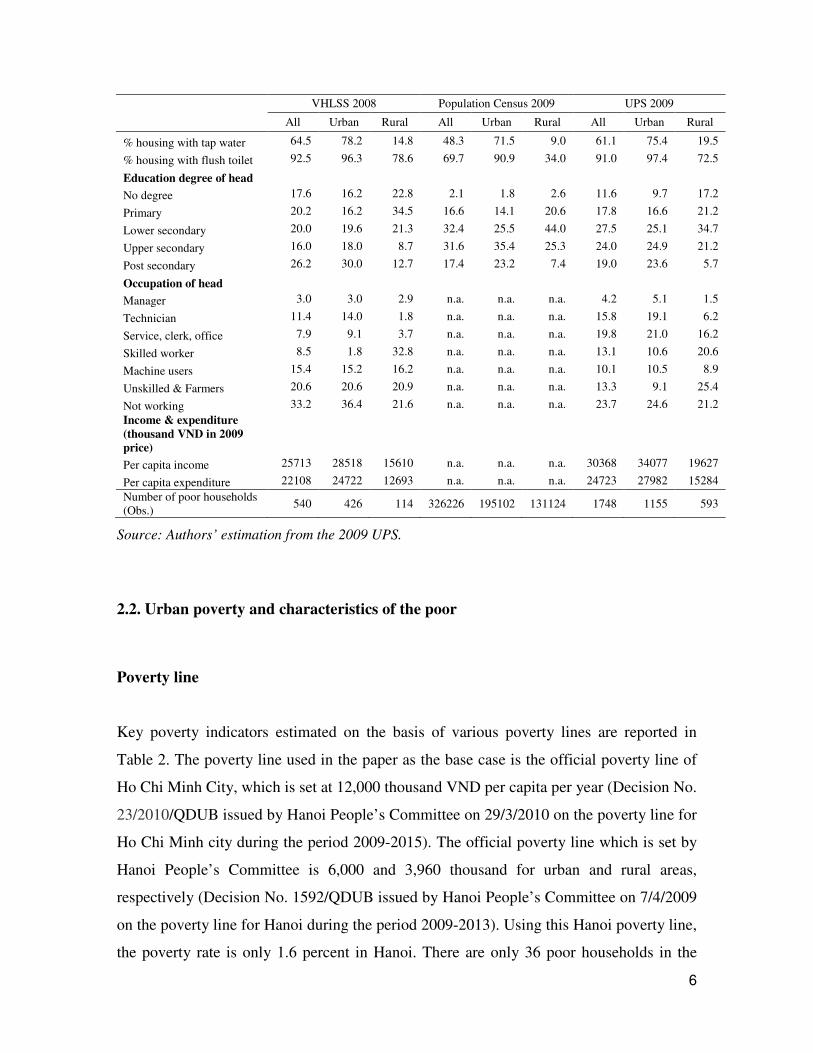
2.3. Relative poverty lines

In addition to the absolute poverty line of per annum income of 12,000 million VND, we

also use the relative poverty lines which define the poor as those having the 5 percent and

10 percent lowest income. The advantage of such relative poverty lines is that results of

analysis are not sensitive to ad hoc defined absolute poverty lines. Table 4 presents the

characteristics of the poor defines using relative poverty lines. Overall the non-poor have

more assets, higher education and better jobs than the poor. They also have better housing

conditions than the poor households.

There is a difference in characteristics of households between Hanoi and HCM

city. The proportion of poor households living in urban areas is lower in Hanoi than in

HCM city. The poor in Hanoi are more likely to have unskilled and farm works than the

poor in HCM city.

The poor in Hanoi have smaller living areas and less access to tap water and flush

toilet than the poor in HCM city. However, the poor in Hanoi are less likely to living a

dormitory than the poor in HCM city.

Table 4: Characteristics of poor and non-poor by relative poverty line

Variable

Hanoi HCM city

5% lowest income

10% lowest income

5% lowest income

10% lowest income

Poor Non-Poor

Poor Non-Poor

Poor Non-Poor

Poor Non-Poor

% household living in urban

areas 29.62 64.96 31.43 66.99 79.15 83.00 70.94 83.97

Without registration book 35.45 23.92 25.97 24.30 42.96 32.38 33.54 32.60

% household members above 60 11.47 9.54 10.60 9.52 11.26 7.14 11.40 6.88

% household members below 15 22.54 16.54 24.68 15.91 13.59 15.91 20.43 15.43

% female members 66.60 53.15 64.30 52.56 49.41 53.25 48.73 53.54

Household size 3.26 3.36 3.41 3.34 2.58 3.14 2.98 3.14


Motorbike 28.47 77.02 42.24 78.48 48.97 77.11 53.91 78.34

Television 55.25 81.48 63.96 82.12 49.00 79.65 67.39 79.82

Computer 0.19 43.82 5.66 45.95 11.39 34.02 9.52 35.53

Fridge 8.40 68.66 24.89 70.55 36.15 57.91 34.03 59.40

Mobile phone 40.75 88.13 53.46 89.64 60.59 87.62 66.98 88.65

Desk telephone 23.84 67.54 41.56 68.24 32.78 48.43 31.20 49.51

Internet connection 0.00 32.30 2.66 34.04 0.00 22.34 1.60 23.52

13

Variable

Hanoi HCM city

5% lowest income

10% lowest income

5% lowest income

10% lowest income

Poor Non-Poor

Poor Non-Poor

Poor Non-Poor

Poor Non-Poor

Housing

Ling in dormitory 7.27 8.41 4.51 8.81 27.51 21.86 22.48 21.98

Living areas per capita (m2) 8.56 17.87 10.97 18.17 18.64 24.71 26.64 24.34

% housing with concrete roof 58.99 78.46 66.09 78.86 15.30 24.39 13.12 25.13

% housing with concrete floor 60.03 88.44 69.66 89.11 89.96 91.18 85.68 91.64

% housing with tap water 13.70 68.25 17.27 71.29 46.40 51.50 45.45 51.88

% housing with flush toilet 34.19 86.68 46.04 88.61 81.79 90.65 82.94 91.08

% households using gas and electricity for cooking

25.50 76.62 36.90 78.52 67.81 86.52 67.58 87.66

Characteristics of household

head

Head single 22.04 14.56 15.91 14.81 46.92 22.24 29.79 22.31

% with male head 50.90 57.16 55.05 57.08 56.59 57.78 51.46 58.31

Age of head 44.49 44.64 43.99 44.71 39.10 42.03 42.04 41.94

Head has been arrived since 2008 34.59 16.04 24.34 16.06 41.29 16.07 27.51 15.82


No degree 24.60 4.55 20.98 3.70 26.13 13.54 26.98 12.71

Primary 19.99 7.55 16.69 7.14 25.02 24.38 34.03 23.53

Lower secondary 43.83 32.67 45.45 31.77 28.77 27.00 24.16 27.31

Upper secondary 11.39 31.32 13.70 32.31 19.54 20.70 14.13 21.25

Post secondary 0.19 23.92 3.17 25.07 0.54 14.39 0.70 15.20

Occupation of head

Manager 0.00 3.27 0.00 3.48 6.91 3.38 2.35 3.59

Technician 0.00 19.16 0.00 20.37 1.65 13.21 1.08 13.95

Service, clerk, office 3.80 15.12 5.32 15.66 12.86 20.90 14.80 21.20

Skilled worker 9.36 14.33 18.35 13.59 16.33 15.26 19.95 14.87

Machine users 3.45 6.84 2.62 7.15 10.03 14.65 7.81 15.13

Unskilled & Farmers 64.06 21.24 55.45 19.54 25.94 14.55 28.82 13.61

Not working 19.32 20.05 18.26 20.22 26.27 18.05 25.19 17.66

Head's employers

State 3.41 20.64 2.64 21.82 0.42 10.27 0.46 10.86

Private 5.14 13.76 8.51 13.91 24.43 22.63 19.99 22.92

Households 70.92 41.20 70.00 39.43 47.17 40.97 52.17 40.15

Foreign 1.21 4.36 0.59 4.63 1.72 8.08 2.19 8.41

Not working 19.32 20.05 18.26 20.22 26.27 18.05 25.19 17.66

Head's work with contract 4.63 36.72 8.39 38.31 18.47 31.50 14.18 32.66

Other household characteristics

Receiving pension (yes = 1) 8.53 25.32 8.31 26.41 6.84 4.09 3.91 4.19

Borrowing (yes =1 ) 35.11 20.36 37.58 19.13 21.27 21.23 36.04 19.89

Receiving remittances (yes = 1) 87.39 79.46 87.25 78.97 30.85 34.94 38.00 34.54

Head having chronic disease 35.19 25.13 31.82 24.88 24.44 18.41 20.71 18.39

Being members of an association 64.27 73.43 62.64 74.20 27.77 50.61 36.47 51.19

14

Variable

Hanoi HCM city

5% lowest income

10% lowest income

5% lowest income

10% lowest income

Poor Non-Poor

Poor Non-Poor

Poor Non-Poor

Poor Non-Poor

% members having health insurance

42.9 62.6 43.6 63.8 28.5 52.9 34.9 53.8

Income

Per capita income (thousand VND)

4728 29023 6610 30341 5125 30048 7523 31316

% income from farm 23.71 4.08 20.69 3.19 2.06 1.13 3.22 0.97

% income from non-farm 5.22 17.42 5.37 18.17 6.09 25.41 15.97 25.67

% income from wage 54.32 57.63 53.83 57.89 71.06 60.65 62.65 60.79

% income from pension 4.46 8.07 3.80 8.37 3.52 0.99 2.02 0.98

% income from other sources 12.3 12.8 16.3 12.4 17.3 11.8 16.1 11.6

Consumption

Per capita expenditure (thousand VND)

5680.0 21528 7253 22347 941 21613 9978 22289

% expenditure on food 53.20 55.23 54.04 55.26 58.96 61.62 64.56 61.27

% expenditure on housing 2.69 5.99 3.27 6.13 8.74 9.06 8.22 9.13

% expenditure on health 4.88 4.65 5.07 4.61 4.18 3.72 4.38 3.67

% expenditure on education 3.43 5.80 4.28 5.85 2.20 4.51 3.98 4.48

% expenditure on transportation 11.14 13.19 10.78 13.36 15.39 11.18 10.75 11.35

% expenditure on other goods 24.66 15.15 22.56 14.79 10.54 9.91 8.11 10.09

Number of obs. 87 1550 167 1470 81 1631 168 1544


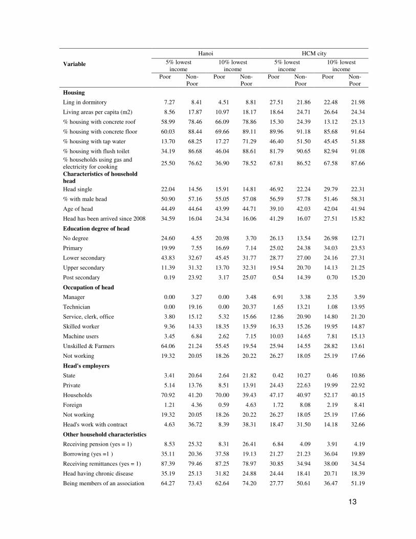
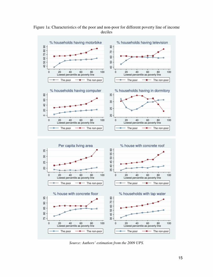
To examine the sensitivity of the poor’s characteristics to the income poverty line,

we use different relative poverty lines which are based on income deciles to define the

poor and compare characteristics between the poor and non-poor. The figure 1a and 1b

present this sensitivity analysis. The horizontal axis is relative poverty lines which are set

from the 10th percentile to the 90th percentile of per capita income. The vertical axis

measures household’s assets, education and occupation of household heads. Several

characteristics including television, living in a dormitory, having registration book are

quite sensitive to the poverty lines. The difference in these variables between the poor and

non-poor varies remarkably as the poverty line increases.

15

Figure 1a: Characteristics of the poor and non-poor for different poverty line of income deciles

40

50

60

70

80

90

0 20 40 60 80 100Lowest percentile as poverty line

The poor The non-poor

% households having motorbike

40

50

60

70

80



% households having television0

20

40

60

80



% households having computer

20

25

30

35



% households having in dormitory

20

25

30

35



Per capita living area

35

40

45

50

55

60



% house with concrete roof

75

80

85

90

95



% house with concrete floor

30

40

50

60

70

80



% households with tap water


16

Figure 1b: Characteristics of the poor and non-poor for different poverty line of income deciles

70

80

90

10

0



% households with flush toilet

45

50

55



% households with registration book20

30

40

50



% heads arriving since 2008

15

20

25

30



% heads upper-secondary school

020

40

60



% heads post-secondary

010

20

30

40



% heads unskilled workers

20

30

40

50

60



% heads working for households

020

40

60

80



% heads working without contract


17

3. Determinants of urban poverty

In this section, we examine the determinants of urban poverty in Hanoi and Ho Chi Minh

City. Previous studies on urban poverty in Vietnam including ActionAid (2009) and Vu

Quoc Huy (2006). However, both studies do not address the determinants of urban

poverty. ActionAid (2009) used data collected from two wards and one commune in Hai

Phong City and two wards in Ho Chi Minh City, incorporating both questionnaires and in-

depth interviews. While providing insight into the current situation of urban poverty in

Vietnam, its low coverage means that the results are hardly useful for in-depth analysis on

the determinants and dynamics of poverty. Vu Quoc Huy (2006) on the other hand, used

Vietnam Household Living Standard (VHLSS) to calculate poverty headcount and poverty

gap in Ha Noi and Ho Chi Minh City. However, the study did little in explaining the

causes of poverty. Moreover, while the VHLSS is a very good data source for general

purposes, its usefulness in analyzing urban poverty is limited because of its small sample

size at the provincial levels. For example, the expenditure module in the VHLSS 2006,

which was normally used to estimate poverty - included only 240 households in Hanoi and

300 households in Ho Chi Minh city.

On the other hand, this study uses Urban Poverty Survey 2009, the most up-to-date

survey implemented in 2009 in Ha Noi and Ho Chi Minh City. The definition of urban

areas used in the survey was adopted from Population and Housing Census of 2009.

3.1. Model specification

To investigate determinants of poverty, we assume the follow function:

( ) ( )βα XGXPIP +== |1 ,

where PI is a binary indicator of poverty status, and X is a vector control variables

including individual and household characteristics which can affect or be associated with

18

poverty status. We use a binomial logistic regression model given that the dependent

variable is dichotomous: 0 when a household is above and 1 when below the poverty line.

The poverty line used in the paper is the official poverty line of Ho Chi Minh City, which

is set at 1 million VND per capita per month. We use income data collected by the survey

to determine if a household is considered poor or not.

Like other earning variables, poverty status can depend on a set of household

characteristics which can be grouped into 5 categories (Glewwe, 1991): (i) Household

composition, (ii) Regional variables, (iii) Human assets, (iv) Physical assets, and (v)

Commune characteristics. In this study, we also include several policy variables to

examine the relation between poverty and social policy variables. The proposed list of

control variables is:

• Household composition: fraction of dependent people, fraction of female, age and

gender of household head.

• Regional variables: dummy variables of HCM city and urban areas

• Human assets: education and occupation of household members, household head.

• Physical assets: housing characteristics, the number of motorbike per household

member.

• Policy variables: chronic disease of heads, registration book, migration and health

insurance.

Efforts will be exerted to identify as many as possible policy variables, either

direct measures or proxies from the dataset, as they are the ones that are under policy

makers’ control and therefore are of special interest. It should be noted that some variables

such as education and employment can be endogenous in equation. Solving endogeneity is

not an easy task, especially without panel data. For these variables, their estimated

coefficients reflect association or correlation between poverty and these variables rather

than the causal effects of these variables on poverty.

The estimates of the logit regressions are shown in Table 5. We use two models:

Model 1 uses relatively exogenous explanatory variables, and Model 2 includes a larger

19

number of explanatory variables including policy variables which are more likely to be

endogenous.

The logit model fitted the data well. The results show that education is an

important determinant of poverty, as also indicated by previous research in developing

countries. Having higher education degrees leads to larger reduction in the probability of

the poverty.

The results show that households with higher proportions of children tend to be

poorer. This result is consistent with economic theory because in these households,

income earned by working household members must be shared to a larger number of

dependents. Households in which the household heads are unmarried tend to be poorer

too. Poor households tend to borrow than non-poor households.

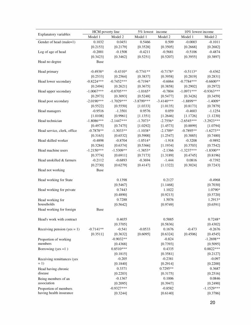
Table 5: Logistic regression of poverty

Explanatory variables HCM poverty line 5% lowest income 10% lowest income

Model 1 Model 2 Model 1 Model 2 Model 1 Model 2

Urban (yes=1) -0.6350*** -0.6975*** -0.5248* -0.6646** -0.5232** -0.5935***

[0.1930] [0.1915] [0.3175] [0.3110] [0.2180] [0.2143]

Hanoi (yes=1) 0.3283* 0.4459** 0.1303 0.0696 0.0446 0.0441

[0.1945] [0.2099] [0.3409] [0.3270] [0.2326] [0.2435]

Without registration book -1.4263*** -1.5382*** -2.4899*** -2.5753*** -1.6112*** -1.6700***

[0.3799] [0.3920] [0.4799] [0.5030] [0.4445] [0.4512]

Head has been arrived since 2008

1.5048*** 1.7107*** 2.5950*** 2.8066*** 1.4406*** 1.6851***

[0.3654] [0.3587] [0.4574] [0.4844] [0.4564] [0.4395]

% household members above 60

0.5693 0.6394 0.9007 0.9017 1.0029* 1.0475*

[0.4817] [0.4936] [0.6649] [0.7317] [0.5414] [0.5647]

% household members below 15

2.4878*** 2.2103*** 2.4099*** 2.2590*** 3.5963*** 3.1672***

[0.5045] [0.5718] [0.7418] [0.8639] [0.6018] [0.6701]

% female members -0.4908 -0.4087 -0.0682 0.0418 -0.4797 -0.443

[0.3058] [0.3124] [0.5067] [0.5252] [0.3820] [0.3955]

Household size 0.0701 0.0719 0.0365 0.0526 0.0366 0.0432

[0.0711] [0.0673] [0.0798] [0.0821] [0.0705] [0.0704]

Having motorbike -1.0991*** -1.0358*** -1.3024*** -1.3132*** -1.2931*** -1.2328***

[0.2475] [0.2500] [0.3137] [0.3238] [0.2793] [0.2771]

Ling in dormitory -0.2758 -0.2173 -0.002 0.0769 -0.0518 0.0227

[0.2722] [0.2716] [0.4186] [0.4167] [0.3168] [0.3215]

Log of living areas per capita (m2)

-0.2268** -0.2365** -0.3525** -0.3747** -0.093 -0.1128

[0.1147] [0.1148] [0.1618] [0.1575] [0.1342] [0.1352]

% housing with concrete floor

0.3824 0.5634** 0.4003 0.4655 -0.0061 0.1434

[0.2899] [0.2831] [0.3840] [0.3784] [0.3204] [0.3120]

% housing with tap water -0.281 -0.3155 -0.1749 -0.1578 -0.178 -0.1693

[0.2008] [0.1931] [0.3908] [0.3580] [0.2359] [0.2203]

% housing with flush toilet -0.4834** -0.5316** -0.7839** -0.7557** -0.5775** -0.6403**

[0.2252] [0.2310] [0.3277] [0.3354] [0.2605] [0.2625]

Head single 0.4433 0.5845** 1.0827** 1.1419*** 0.5710* 0.7466**

[0.2792] [0.2827] [0.4402] [0.4346] [0.3176] [0.3137]

20



Gender of head (male=1) 0.1032 0.0451 0.5466 0.509 -0.0003 -0.1011

[0.2153] [0.2179] [0.3528] [0.3505] [0.2668] [0.2682]

Log of age of head -0.2001 -0.1508 -0.4211 -0.5681 -0.5106 -0.4874

[0.3423] [0.3462] [0.5251] [0.5207] [0.3955] [0.3897]

Head no degree Base

Head primary -0.4938* -0.4310* -0.7741** -0.7178* -0.5113* -0.4362

[0.2533] [0.2564] [0.3837] [0.3958] [0.2819] [0.2831]

Head lower secondary -0.8224*** -0.7452*** -0.7194* -0.6064 -0.7784*** -0.6600**

[0.2494] [0.2621] [0.3675] [0.3858] [0.2902] [0.2972]

Head upper secondary -1.0067*** -0.8705*** -1.0165* -0.7804 -1.0971*** -0.9363***

[0.2973] [0.3093] [0.5248] [0.5477] [0.3426] [0.3459]

Head post secondary -2.0190*** -1.7029*** -3.8799*** -3.4140*** -1.8899** -1.4009*

[0.5522] [0.5550] [1.0333] [1.0135] [0.8173] [0.7879]

Head managers -0.9516 -1.3501 0.9576 0.059 -0.4603 -1.1254

[1.0108] [0.9961] [1.1351] [1.2646] [1.1726] [1.1230]

Head technician -1.8086*** -2.1447*** -1.7073* -2.7556* -2.6545*** -3.2923***

[0.4975] [0.7475] [1.0292] [1.4573] [0.8899] [1.0794]

Head service, clerk, office -0.7878** -1.3033** -1.1038* -2.1709* -0.7895** -1.6273**

[0.3163] [0.6532] [0.5900] [1.2547] [0.3885] [0.7480]

Head skilled worker -0.4898 -0.8704 -1.0514* -1.918 -0.3208 -0.9892

[0.3284] [0.6374] [0.5366] [1.1934] [0.3703] [0.7542]

Head machine users -1.2150*** -1.5309** -1.3853* -2.1366 -1.3237*** -1.8300**

[0.3774] [0.6911] [0.7173] [1.3189] [0.4745] [0.8196]

Head unskilled & farmers -0.2112 -0.6893 -0.3694 -1.444 0.0816 -0.7392

[0.2730] [0.6279] [0.4147] [1.1322] [0.3024] [0.7243]

Head not working Base

Head working for State

0.1398

0.2127

-0.4968

[0.5467]

[1.1468]

[0.7030]

Head working for private

0.7443

1.1022

1.0790*

[0.4890]

[0.9213]

[0.5720]

Head working for households

0.7288

1.5076

1.2913*

[0.5642]

[0.9749]

[0.6591]

Head working for foreign Base

Head's work with contract

0.4655

0.5885

0.7248*

[0.3705]

[0.5836]

[0.4302]

Receiving pension (yes = 1) -0.7141** -0.541 -0.0533 0.1676 -0.473 -0.2676

[0.3511] [0.3632] [0.6095] [0.6324] [0.4506] [0.4545]

Proportion of working members

-0.9032**

-0.824

-1.2698**

[0.4368]

[0.7393]

[0.5095]

Borrowing (yes =1 )

0.8510***

0.4335

0.8822***

[0.1815]

[0.3581]

[0.2127]

Receiving remittances (yes = 1)

-0.205

-0.2381

-0.097

[0.1840]

[0.2914]

[0.2200]

Head having chronic disease

0.3371

0.7295**

0.3687

[0.2203]

[0.3175]

[0.2516]

Being members of an association

-0.1367

0.1006

0.0846

[0.2095]

[0.3947]

[0.2490]

Proportion of members having health insurance

-0.9327***

-0.8582

-1.1529***

[0.3244]

[0.6140]

[0.3786]

21



Constant 1.6062 1.7988 0.8236 1.5387 2.1441 2.491

[1.4491] [1.4874] [2.0628] [2.1676] [1.6606] [1.6889]

Observations 3349 3349 3349 3349 3349 3349

R-squared 0.22 0.25 0.24 0.26 0.23 0.27

Robust standard errors in brackets * significant at 10%; ** significant at 5%; *** significant at 1%


Health problems, indicated by sickness or chronic disease, is a determinant of

poverty when the lowest 5% percentiles of income is use a relative poverty line. However,

the effect of health problems is not statistically significant in other models. The effect of

having health insurance significantly lower the probability of being poor, perhaps by

lowering the health financing burden to the households. Receiving pension is negatively

associated with lower probability of being poor. This result is consistent with Long and

Pfau (2009) who found that receiving social security benefit, which for the most part is

pension, is significantly associated with lower probability of being poor for elderly people

in Vietnam. On the other hand, receiving remittance seems have no effect on poverty and

borrowing increases the likelihood of a household falling into poverty.

Occupation has significant effect on poverty. Generally, a household whose

household head work in the private sector is more likely to be poor than those households

whose heads work in the State or the foreign-invested sector. Similarly, agricultural

households are more likely to be poor than those households in the industrial or service

sector.

Regional variables have statistically significant effect in when the income poverty

line is 12,000 thousand VND/person/month. Households in Ho Chi Minh City and in the

inner cities are less likely to be poor than the ones in Hanoi and in the suburban,

respectively.

It is interesting the variable of ‘without registration book’ is negatively correlated

with poverty, but the recent migration to city is positive correlated with poverty. This

implies that recent migrants are more likely to be poor, but permanent migrants can tend

to be non-poor.

22

3.3. Determinants of urban income and expenditures

While it is important to determine the factor influencing poverty, it is also necessary to

know the factors determining household income per capita as well as expenditure per

capita in urban areas. To investigate household and individual characteristics associated

with income and expenditure, the following function of per capita income (and also per

capita expenditure):

εβα ++= XY )ln( ,

where Y is per capita income, and X is a vector control variables which are similar as in

the above equation of poverty. Again some explanatory variables in the income equation

can be endogenous. For these variables, their estimated coefficients reflect association or

correlation between poverty and these variables.

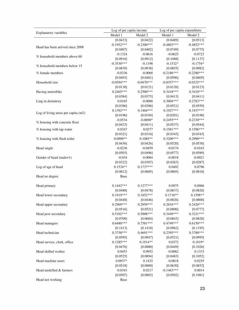
Table 6 summarizes the determinants of urban income as well as expenditure in

Hanoi and Ho Chi Minh City. The dependent variable is the log of income/expenditure per

capita. Independent variables are similar to those in Table 5.

Table 6 indicates that most of the coefficients that determine poverty are also

significant in explaining urban household income and expenditure per capita. In particular,

inner city, Ho Chi Minh City and education have positive impacts on both household

income and expenditure per capita. On the other hand, households with larger household

size and higher proportions of elderly, children and females are more likely to have lower

income or expenditure. Households whose heads work for wage or agriculture receive

lower income or expenditure. In addition, households whose heads are working have

higher income/expenditure than those whose heads are not working.

Table 6: Determinants of urban income and consumption expenditure

Explanatory variables Log of per capita income Log of per capita expenditure

Model 1 Model 2 Model 1 Model 2

Urban 0.2077*** 0.2183*** -0.0043 0.0194

[0.0322] [0.0317] [0.0399] [0.0384]

Hanoi (yes=1) -0.0316 -0.0254 -0.0575 -0.0595

[0.0310] [0.0324] [0.0368] [0.0391]

Without registration book 0.1991*** 0.1507*** 0.1182** 0.1189**

23



[0.0433] [0.0422] [0.0489] [0.0513]

Head has been arrived since 2008 -0.1952*** -0.2300*** -0.4803*** -0.4852***

[0.0407] [0.0402] [0.0749] [0.0775]

% household members above 60 -0.1324 -0.0616 -0.0625 -0.0723

[0.0916] [0.0912] [0.1088] [0.1137]

% household members below 15 -0.3530*** -0.1198 -0.1532* -0.1754*

[0.0839] [0.0938] [0.0855] [0.0982]

% female members -0.0336 -0.0068 -0.2186*** -0.2280***

[0.0493] [0.0481] [0.0596] [0.0605]

Household size -0.0594*** -0.0470*** -0.0357*** -0.0325***

[0.0130] [0.0121] [0.0126] [0.0123]

Having motorbike 0.2465*** 0.2500*** 0.3418*** 0.3410***

[0.0384] [0.0375] [0.0413] [0.0411]

Ling in dormitory 0.0165 -0.0088 0.3004*** 0.2783***

[0.0386] [0.0386] [0.0521] [0.0559]

Log of living areas per capita (m2) 0.1392*** 0.1404*** 0.1927*** 0.1937***

[0.0196] [0.0194] [0.0201] [0.0198]

% housing with concrete floor -0.0534 -0.0690* 0.2455*** 0.2330***

[0.0423] [0.0411] [0.0537] [0.0544]

% housing with tap water 0.0247 0.0277 0.1581*** 0.1596***

[0.0321] [0.0316] [0.0343] [0.0343]

% housing with flush toilet 0.0909** 0.1085** 0.3209*** 0.2990***

[0.0436] [0.0426] [0.0520] [0.0538]

Head single -0.0236 -0.0459 -0.0174 -0.0163

[0.0503] [0.0496] [0.0577] [0.0589]

Gender of head (male=1) -0.034 -0.0084 -0.0018 -0.0021

[0.0322] [0.0307] [0.0283] [0.0287]

Log of age of head 0.1534** 0.1737*** 0.0492 0.0796

[0.0612] [0.0605] [0.0805] [0.0818]

Head no degree Base

Head primary 0.1442*** 0.1277*** 0.0975 0.0966

[0.0488] [0.0478] [0.0837] [0.0826]

Head lower secondary 0.1919*** 0.1852*** 0.1710** 0.1598**

[0.0448] [0.0446] [0.0826] [0.0800]

Head upper secondary 0.2969*** 0.2959*** 0.2654*** 0.2420***

[0.0516] [0.0521] [0.0806] [0.0777]

Head post secondary 0.5102*** 0.5008*** 0.3449*** 0.3221***

[0.0709] [0.0684] [0.0843] [0.0828]

Head managers 0.6480*** 0.7581*** 0.4749*** 0.6150***

[0.1413] [0.1418] [0.0962] [0.1195]

Head technician 0.3758*** 0.4691*** 0.2395*** 0.3780***

[0.0595] [0.0947] [0.0521] [0.0995]

Head service, clerk, office 0.1285*** 0.1914** 0.0372 0.1819*

[0.0476] [0.0880] [0.0449] [0.1026]

Head skilled worker 0.0453 0.0952 -0.0062 0.1333

[0.0525] [0.0894] [0.0483] [0.1052]

Head machine users 0.0937* 0.1432 -0.0818 0.0255

[0.0518] [0.0880] [0.0630] [0.0852]

Head unskilled & farmers -0.0343 0.0217 -0.1483*** 0.0014

[0.0507] [0.0883] [0.0502] [0.1081]

Head not working Base

24



Head working for State

-0.2278***

-0.2134***

[0.0575]

[0.0671]

Head working for private

-0.1249**

-0.0332

[0.0514]

[0.0556]

Head working for households -0.1669**

-0.1535*

[0.0741]

[0.0915]

Head working for foreign Base

Head's work with contract

-0.0902

0.0056

[0.0605]

[0.0591]

Receiving pension (yes = 1) 0.0901* 0.0956** 0.0317 0.0254

[0.0469] [0.0456] [0.0440] [0.0445]

Proportion of working members

0.4566***

0.0032

[0.0746]

[0.0702]

Borrowing (yes =1 )

-0.1181***

0.0301

[0.0308]

[0.0289]

Receiving remittances (yes = 1) 0.0391

0.0568*

[0.0273]

[0.0310]

Head having chronic disease -0.0705**

-0.0406

[0.0330]

[0.0461]

Being members of an association -0.0866***

-0.0105

[0.0318]

[0.0308]

Proportion of members having health insurance

0.1245**

0.0524

[0.0484]

[0.0463]

Constant 8.6171*** 8.2500*** 8.2388*** 8.0879***

[0.2625] [0.2673] [0.3029] [0.3145]

Observations 3349 3349 3349 3349

R-squared 0.39 0.43 0.42 0.42

Standard errors in brackets * significant at 10%; ** significant at 5%; *** significant at 1%


4. Dynamic aspects of urban poverty

4.1. Methodology

It is difficult to investigate poverty dynamics without panel data. In principle the

chronically poor are households whose living standard is below a defined poverty line for

a period of several years, while the transiently poor experience some non-poverty years

during that period (Hulme and Shepherd, 2003). Even with a widely used approach by

(Jalan and Ravallion, 2000) in which poverty is decomposed into two components: the

25

transient poverty due to the intertemporal variability in consumption, and the chronic

poverty simply determined by the mean consumption overtime, longitudinal data with at

least three repeated observations are required to estimate the chronic and transient poverty.

Unfortunately these kinds of data are not available for urban poverty analysis.

In this study, a variant of poverty dynamics approach by Carter and May (2001)

will be used to decompose poverty into structural and stochastic poverty. To incorporate

the aspect of poverty dynamics into this definition, let’s start with a simple economic

model of intertemporal choice in two periods t and t+1. It is assumed that a households i at

the time t has a vector of assets, Ait that includes physics, human and also social capitals.

At the period t households i is assumed to choose consumption (cit) and investment (Iit) to

maximize their expected welfare. It is expressed in the following form:

)()( max)( )1(

*

},{c

*

it++≡ tiit

Iit AJcuAJ

it

subject to:

0

),(

)1(

)1(

≥

Θ−+=

−=

+

+

ti

itititti

itititit

A

IAA

IAFc θ

where J*(Ait) defines the maximum discounted stream of future livelihood that household i

expects given a starting asset endowment Ait and optimal future behavior. When

optimizing the welfare the household faces three constraints. The fist is the budget

constraint given by income F(Ait, θit), a function of assets Ait and the stochastic income

shock θit. The second constraint shows that the future asset endowment can be reduced

due to stochastic asset shocks Θit. The last constraint assumes that the assets are non-

negative, i.e. the household cannot borrow.

Under the usual assumption of diminishing marginal utility of consumption, the

household would prefer smoothness rather than fluctuation in consumption over two

periods. In order to smooth consumption the household must have perfect access to credit

market. The household also would like to borrow in event of income shocks θit, or asset

shocks Θit. However such a credit market is not available for the poor, especially in

developing countries. The way they can cope with adverse shocks is to track their assets.

26

If a large amount of assets is sold, the remaining assets might not be sufficient to generate

income sufficient to sustain not only investment but also consumption in next period. The

household can fall into poverty, even poverty trap.

With a note that there is no obvious evidence of consumption smoothing by the poor,

Carter and May (2001) decompose the realized (current) consumption, cit into three

following components:

ititiit Accc ε++= )(0 .

The first component c0i is the steady consumption based on permanent income that the

household would enjoy if they can smooth the consumption. Facing the binding borrowing

constraint the household might track the current asset c(Ait), and the third term εit will

become non-zero when the household cannot smooth out shocks. If the household can

maintain stable consumption the two later terms in the right-hand side of (4) will be zero.

Because the permanent income is generated based on the assets, the first two terms can be

grouped into the expected consumption for household i, denoted by �(Ait).

Now denote the money metric poverty line as cPL, and a household is classified

poor if their realized consumption is below the poverty line. Carter and May (1999)

estimate the asset poverty line, APL that satisfies the following condition:

{ }PLPLPL cAcAA == )(ˆ| .

The asset poverty line APL is the combination of assets that are expected to yield the level

of welfare equal to the poverty line cPL. A poor household is defined as structurally poor if

their asset level is lower than the asset poverty line. The stochastically poor are those

whose asset level is above the asset poverty line. Levels of assets that are higher than the

asset poverty line are expected to generate consumption level above the poverty line cPL in

next period. Thus the stochastically poor can find it easier to escape poverty.

Once the asset poverty line is estimated, one can classify the population into four

groups: the structurally and stochastically poor, the stochastically and structurally non-

poor. Households are defined as structurally poor if they are observed to be poor and their

asset level places them below the poverty line. Households who are poor in terms of their

realized living standard but have asset level above the asset poverty line are called

27

stochastically poor. The stochastically non-poor households are those who are non-poor

but have their asset level below the asset poverty line. Finally, the structurally non-poor

households are those who are non-poor and have asset level above the poverty line.

4.2. Estimation results

To estimate the asset level of each household, the first step is to run regression of per

capita income on asset variables which are expected to generate income of the households

in the long-term. Then the predicted per capita income is estimated for each household in

the sample. This expected per capita income can be regarded as long-term income which

depends on the asset level. Thus it can be a proxy for the asset level of households. The

income model is similar to Model 1 in Table 6, but the dependent variable is per capita

income instead of log of per capita income. It is assumed that households cannot change

the level of these assets at least in short-term. We estimate different models. The estimates

of structural and stochastic poverty rates are very similar across models. We use estimates

from the first model of all the sample for interpretation.

Table 7: The percentage of the poor

Cities Poor Structurally

poor Stochastically

poor Stochastically

non-poor Structurally

non-poor

The poverty line of HCM city

Hanoi 17.38 7.81 9.57 6.96 75.39

HCM city 12.52 2.44 10.09 5.90 80.18

All 14.21 4.30 9.91 6.27 78.52

Poverty line: the lowest 10% income

Hanoi 7.57 2.92 4.65 4.37 88.06

HCM city 3.65 0.32 3.33 4.69 91.65

All 5.01 1.22 3.79 4.58 90.41

Poverty line: the lowest 20% income

Hanoi 12.08 5.12 6.97 5.69 82.23

HCM city 9.02 1.12 7.90 5.40 85.58

All 10.08 2.51 7.57 5.50 84.41


Table 7 shows the estimation of different types of poverty. There is a large

proportion of the poor who are found stochastically poor. It is noted that the poverty rate

is equal to sum of the structural poverty and stochastic poverty rates. For both absolute

28

and relative poverty lines, Hanoi has higher rates of structurally poverty than HCM city.

The proportion of structurally poor and stochastically non-poor is rather small. This

poverty structure can be different from the rural poverty structure. Chronic poverty or

structural poverty can be much higher in poor areas, especially in mountainous areas.

5. Inequality

Inequality is expected to become increasingly a big policy issue in urban areas in the next

decade, when Vietnam becomes a low middle income country. The Gini coefficient index

is the most commonly used inequality index in the literature and in practice. The Gini

index is defined as a ratio of the areas on the Lorenz curve diagram. If the area between

the line of perfect equality and the Lorenz curve is A, and the area under the Lorenz curve

is B, then the Gini index is A/(A+B). Since A+B = 0.5, the Gini index, G = A/(0.5) = 2A =

1-2B. Practically, the Gini index can be calculated from the individual income in the

population:

��= =

−−

=n

i

n

j

ji YYYnn

G1 1)1(2

1

where Y is the average per capita income or expenditure. The value of the Gini coefficient

varies from 0 to 1. The closer the Gini coefficient is to one, the more unequal is income or

expenditure distribution.

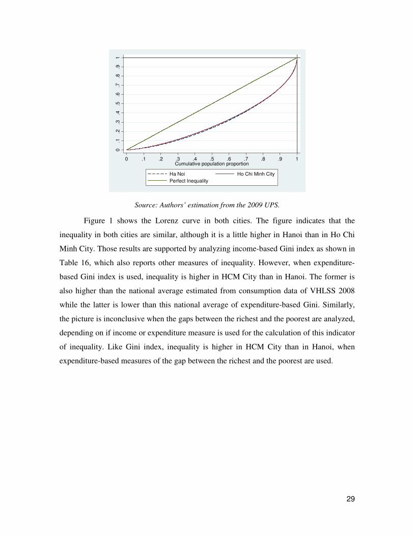
Figure 1: Lorenz curve in Ho Chi Minh city and Hanoi

29

0.1

.2.3

.4.5

.6.7

.8.9

1

0 .1 .2 .3 .4 .5 .6 .7 .8 .9 1Cumulative population proportion

Ha Noi Ho Chi Minh City

Perfect Inequality


Figure 1 shows the Lorenz curve in both cities. The figure indicates that the

inequality in both cities are similar, although it is a little higher in Hanoi than in Ho Chi

Minh City. Those results are supported by analyzing income-based Gini index as shown in

Table 16, which also reports other measures of inequality. However, when expenditure-

based Gini index is used, inequality is higher in HCM City than in Hanoi. The former is

also higher than the national average estimated from consumption data of VHLSS 2008

while the latter is lower than this national average of expenditure-based Gini. Similarly,

the picture is inconclusive when the gaps between the richest and the poorest are analyzed,

depending on if income or expenditure measure is used for the calculation of this indicator

of inequality. Like Gini index, inequality is higher in HCM City than in Hanoi, when

expenditure-based measures of the gap between the richest and the poorest are used.

30

Table 8: Inequality indexes in Hanoi and Ho Chi Minh city

Estimate S.e. Lower bound Upper bound

Expenditure Gini Index

Hanoi 0.326 0.009 0.308 0.344

Ho Chi Minh City 0.432 0.071 0.292 0.571

All 0.400 0.052 0.297 0.503

Income Gini Index

Hanoi 0.398 0.016 0.366 0.43

Ho Chi Minh City 0.386 0.019 0.349 0.424

All 0.391 0.014 0.365 0.418

Duclos Esteban and Ray Index of polarization (2004)

Polarization measure for incomes

Hanoi 0.240 0.010 0.220 0.261

Ho Chi Minh City 0.242 0.010 0.221 0.263

All 0.241 0.007 0.226 0.255

Polarization measure for

expenditure

Hanoi 0.250 0.043 0.165 0.335

Ho Chi Minh City 0.208 0.006 0.196 0.220

All 0.276 0.066 0.145 0.408


Table 9: Income/expenditure gap

Income Expenditure

Mean Median Mean Median

Top 5%/Bottom 5%

Hanoi 21.48 17.26 12.89 9.62

Ho Chi Minh City 21.69 14.34 32.47 10.06

All 21.64 14.78 26.22 9.93

Top 10%/Bottom 10%

Hanoi 12.72 9.07 7.79 6.29

Ho Chi Minh City 11.93 8.13 15.13 5.84

All 12.24 8.61 12.63 6.12

Top 20%/Bottom 20%

Hanoi 6.84 4.80 4.96 4.00

Ho Chi Minh City 6.77 4.80 7.61 3.62

All 6.78 4.75 6.61 3.79


The income Gini estimate in Ho Chi Minh City is 0.386, a little lower than in Ha

Noi (0.398). Meanwhile, the income Gini index for both cities is 0.391. Thus, we can

conclude that there is little difference in income inequality between the two cities.

On the other hand, the expenditure Gini estimate in Ho Chi Minh City is 0.432,

much higher than the one in Hanoi (0.326), Thus, we can conclude that expenditure

31

inequality in Ho Chi Minh City is quite high, and much higher than in Hanoi although the

income inequality in both cities are similar.

The Gini estimate in Ho Chi Minh City is 0.383, a little lower than in Ha Noi

(0.393). Meanwhile, the Gini index for both cities is 0.385. In order to understand the

underlying factors of Gini index, we decompose the Gini Index by income sources using

the approach first proposed by Rao (1969)4. The results in Table 14 shows that in both

cities, differences in wages are the most important factor creating inequality in income,

contributing about 47.8 percent of the Gini index in Hanoi and 42.6 percent in Ho Chi

Minh City. Next to wages, non-farm self-employed income is a major source of income

inequality, contributing 27.3 percent of the Gini index in Hanoi and 41.3 percent in Ho

Chi Minh City. On the other hand, pension and other income are more important

contribution to the Gini index in Hanoi (6.6 percent and 21.8 percent respectively) than in

Ho Chi Minh city (0.85 percent and 15.1 percent respectively).

It is interesting to compare the decomposition of the Gini Index between the two

cities. Non-farm self-employed income plays a much more important role in explaining

income disparity in Ho Chi Minh City than in Hanoi. On the other hand, pension and other

income are more important in Hanoi than in Ho Chi Minh City in contributing to income

disparity. Thus, public policies aimed at reducing inequality should take into account

those differences.

Table 10: Decomposition of the Gini index by income sources

Hanoi HCM city All sample

Income share (%)

Contribution to Gini Index

(%)

Income share (%)

Contribution to Gini Index

(%)

Income share (%)

Contribution to Gini

Index (%)

Non-farm self-enployed income

23.20 27.30 33.47 41.31 31.25 38.02

Service income 0.01 -0.02 0.02 -0.03 0.02 -0.03

Pension 8.13 6.63 1.21 0.85 2.70 2.29

Allowance 0.31 -0.23 0.34 0.16 0.33 0.07

Farm income 2.49 -3.26 0.87 -0.01 1.22 -0.76

Other income 15.74 21.78 12.37 15.13 13.10 16.61

Wages 50.11 47.81 51.72 42.58 51.38 43.80


4 Rao, V.M. (1969), “Two Decompositions of Concentration Ratio” Journal of the Royal Statistical Society, Series A 132, 418-425.

32

6. Conclusions

This study examines determinants of poverty in urban Vietnam and proposes policy

implications for urban poverty reduction. More specifically, it aims to examine several

issues: (i) poverty estimation for Hanoi and HCM city (ii) analysis of sensitivity of

poverty estimates and characteristics of the poor to the selection of poverty lines (iii)

determinants of urban poverty, (iv) dynamic aspects of urban poverty, (v) income and

consumption inequality in urban Vietnam. Data used in this study are from the 2009

Urban Poverty Survey.

Using the poverty line of 12,000 thousand VND/year, the poverty incidence in

Hanoi and Ho Chi Minh city is 17.4 percent and 12.5 percent, respectively. Although

Hanoi has higher poverty than Ho Chi Minh city, Hanoi has higher per capita income than

Ho Chi Minh city. This is because the income inequality is higher in Hanoi than in Ho Chi

Minh city. The income Gini estimate in Ho Chi Minh City is 0.386, lower than in Ha Noi

(0.398). However, Ho Chi Minh city has higher consumption expenditure than Hanoi. In

addition, the expenditure Gini estimate in Ho Chi Minh City is 0.432, much higher than

the one in Hanoi (0.326).

There is a large proportion of the poor who are found stochastically poor. Hanoi

has higher rates of structurally poverty than HCM city. The proportion of structurally poor

and stochastically non-poor is rather small.

Overall the non-poor have more assets than the poor. The proportion of the non-

poor having computer, internet connection, and fridge is much higher than the poor. The

poor have poorer housing conditions, especially they have much lower access to tap water

than the non-poor. There are only nearly 40 percent of the poor households using tap

water, while the non-poor having tap water is around 61 percent. Heads of the poor

households tend to have lower education and unskilled works than the heads of the non-

poor households.

33

References

Carter, M., and May, J. (1999), “Poverty, Livelihood and Class in Rural South Africa”,

World Development, Vol.27, No. 1.

Carter, M., and May, J. (2001), “One Kind of Freedom: Poverty Dynamics in Post-

apartheid South Africa”, World Development, Vol. 29, No. 12.

Dollar, D. and Kraay, A. (2000), Growth Is Good for the Poor, Development Research

Group, Washington, D.C., World Bank.

Easterly, W. and A. Kraay (2000), “Small States, Small Problems? Income, Growth, and

Volatility in Small States”, World Development, Vol. 28, n11, pp. 2013-27.

Glewwe, P (1991). "Investigating the Determinants of Household Welfare in Cote

d'Ivoire." Journal of Development Economics 35: 307-37.

Harrison, Anne (2005), “Globalization and Poverty”, National Bureau of Economic

Research Conference Report, edited by Harrison Anne, Chicago University Press.

Hulme, D., and Shepherd, A. (2003), “Conceptualizing Chronic Poverty”, World

Development, Vol. 31, No 3.

ILO (2008), “Underpaid, Overworked and Overlooked: The realities of young migrant

workers in Thailand”, International Labour Organization 2006.

Jalan, J., and Ravallion, M. (2000), “Is Transient Poverty Different? Evidence for Rural

China”, Journal of Development Studies (Special Issue) (August)

McCulloch, N.; L. A. Winters and X Cirera (2001), “Trade Liberalization and Poverty: A

Handbook”, London, Centre for Economic Policy Research.

Winters Alan, McCulloch, and Andrew McKay (2004), “Trade Liberalization and

Poverty: The Evidence So Far”, Journal of Economic Literature, Vol. XLII (March 2004).

World Bank (2004), “Vietnam Development Report: Poverty”, World Bank in Vietnam.

Duclos, J.‐Y., J. Esteban, and D. Ray (2004): “Polarization: Concepts, Measurement,

Estimation,” Econometrica, 72, 1737–1772.

34

Rao, V.M. (1969), “Two Decompositions of Concentration Ratio” Journal of the Royal

Statistical Society, Series A 132, 418-425.

Long, G.T. and W. Pfau (2009), “The Vulnerability of the Elderly Households to Poverty:

Determinants and Policy Implications for Vietnam,” Asian Economic Journal, Vol. 23,

No. 4, pp. 419-437, December 2009

Vu Quoc Huy (2006) “Urban Poverty: The Case of Vietnam”

Oxfam and ActionAid Vietnam (2009), “Participatory Monitoring of Urban Poverty in

Vietnam.” Synthesis Report 2008.

urban poverty in vietnam: determinants and policy implications · 2019-09-27 · vu hoang linh...

Documents