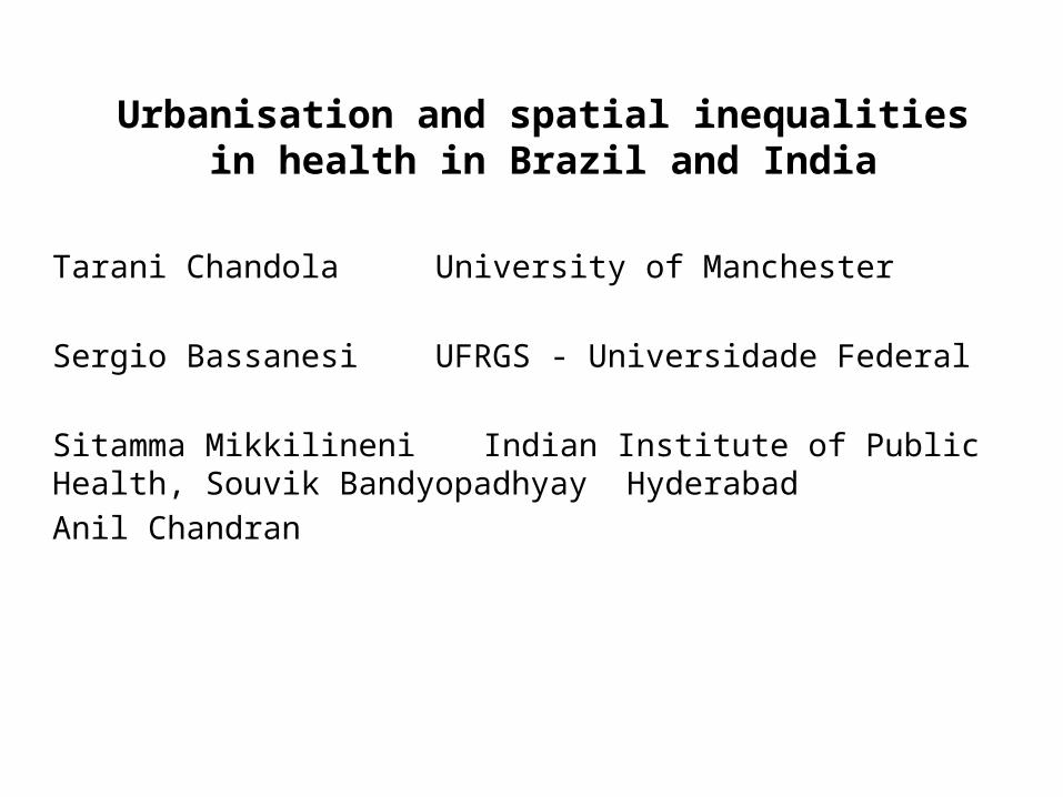
Urbanisation and spatial inequalities in health in Brazil and India

Tarani Chandola University of Manchester

Sergio Bassanesi UFRGS - Universidade Federal

Sitamma Mikkilineni Indian Institute of Public Health, Souvik Bandyopadhyay HyderabadAnil Chandran

Health is related to income differences within rich societies but not to those between them

Within societiesBetween (rich) societies

Source: Wilkinson & Pickett, The Spirit Level (2009)

70

71

72

73

74

75

76

77

78

79

80

Electoral wards in England & Wales ranked by deprivation score

Life

exp

ecta

ncy

(yea

rs)

Mostdeprived

www.equalitytrust.org.uk

Life expectancy and income inequality: Brazil, 2000

 Plot showing the odds ratios (ORs) and 95% confidence interval (CI) for one-standard deviation change in Gini coefficient for the risk of being underweight, pre-overweight,

overweight and obese.

Subramanian S V et al. J Epidemiol Community Health 2007;61:802-809

©2007 by BMJ Publishing Group Ltd

Increasing income inequality in Brazil and India

Increasing spatial inequality in poverty and income- urbanisation and concentration of economic activity- spatial concentration of affluence reproduces privileges of the rich- spatial concentration of poverty results in segregation, involuntary clustering in ghettos

Effects on Individual and Population Health?“Triple health jeopardy: being poor in a poor neighbourhood that is spatially isolated from life-enhancing opportunities…” Nancy A Ross

Dimensions of spatial segregationSean F. Reardon & David O'Sullivan. “Measures of Spatial Segregation” Sociological Methodology. V. 34, n.1, p. 121-162, 2004

EVENNESS

CLUSTERING

EXPOSURE ISOLATION

SPATIAL EXPOSURE INDEX

SPATIAL ISOLATION INDEX

Average proportion of group n in the localities of each member of group m

Average proportion of group m in the local environments of each member of group m (spatial exposure of group m to itself)

EXPOSURE/ISOLATION DIMENSION

SPATIAL NEIGHBOURHOOD SORTING INDEX

Proportion of the variance between the different localities that contributes to the total variance of the variable X in the city

EVENNESS/ CLUSTERING DIMENSION

GENERALIZED SPATIAL DISSIMILARITY INDEX

Average difference of the population composition of the localities from the population composition of the urban area as a whole

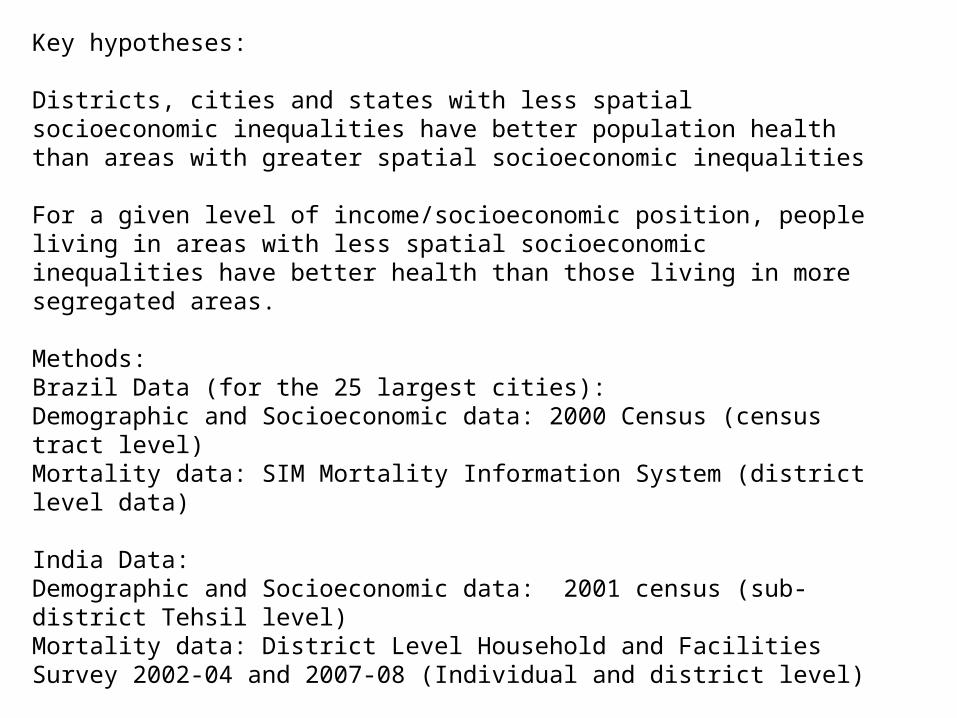
Key hypotheses:

Districts, cities and states with less spatial socioeconomic inequalities have better population health than areas with greater spatial socioeconomic inequalities

For a given level of income/socioeconomic position, people living in areas with less spatial socioeconomic inequalities have better health than those living in more segregated areas.

Methods:Brazil Data (for the 25 largest cities):Demographic and Socioeconomic data: 2000 Census (census tract level)Mortality data: SIM Mortality Information System (district level data)

India Data:Demographic and Socioeconomic data: 2001 census (sub-district Tehsil level)Mortality data: District Level Household and Facilities Survey 2002-04 and 2007-08 (Individual and district level)

Dimensions of spatial segregation

EVENNESS

CLUSTERING

EXPOSURE ISOLATION

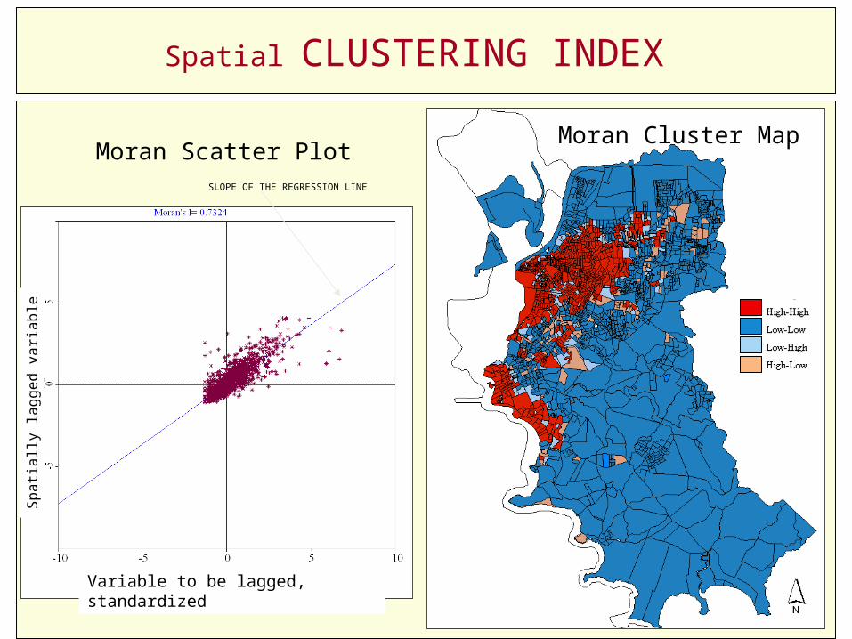
Spatial CLUSTERING INDEX

Moran Scatter PlotSLOPE OF THE REGRESSION LINE

Spati

ally

lagg

ed v

aria

ble

Variable to be lagged, standardized

Moran Cluster Map

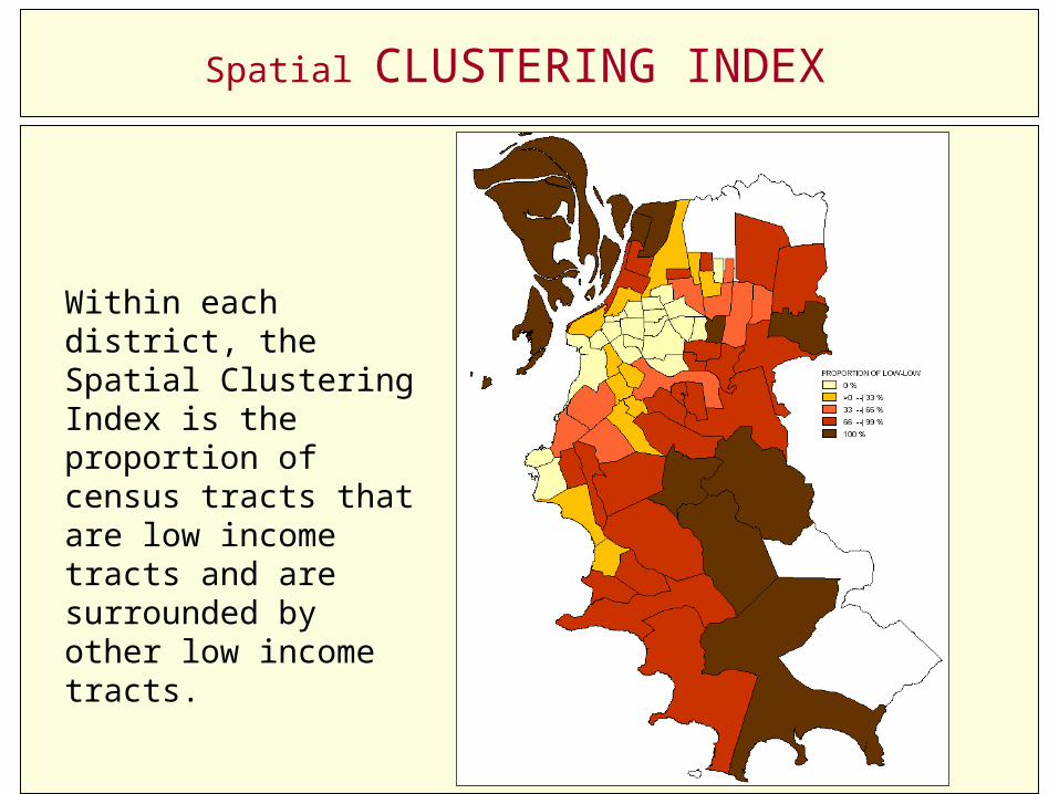
Spatial CLUSTERING INDEX

Within each district, the Spatial Clustering Index is the proportion of census tracts that are low income tracts and are surrounded by other low income tracts.

Dimensions of spatial segregation

EVENNESS

CLUSTERING

EXPOSURE ISOLATION

Spatial Isolation Index Income >20 ms BW:400m

LOCALGLOBAL Ŏ>20=0.228

p<0.01

Local

Spatial Isolation Indexes

Income Groups

BW:400mms: minimum salaries

>20 ms 10-20 ms

5-10 ms<2ms 2-5 ms

INCOME

Moran I Index: 0.65 ( ρ< 0.0001)

Distribution of income of the head of the household by district, Porto Alegre, 2000.Source: IBGE

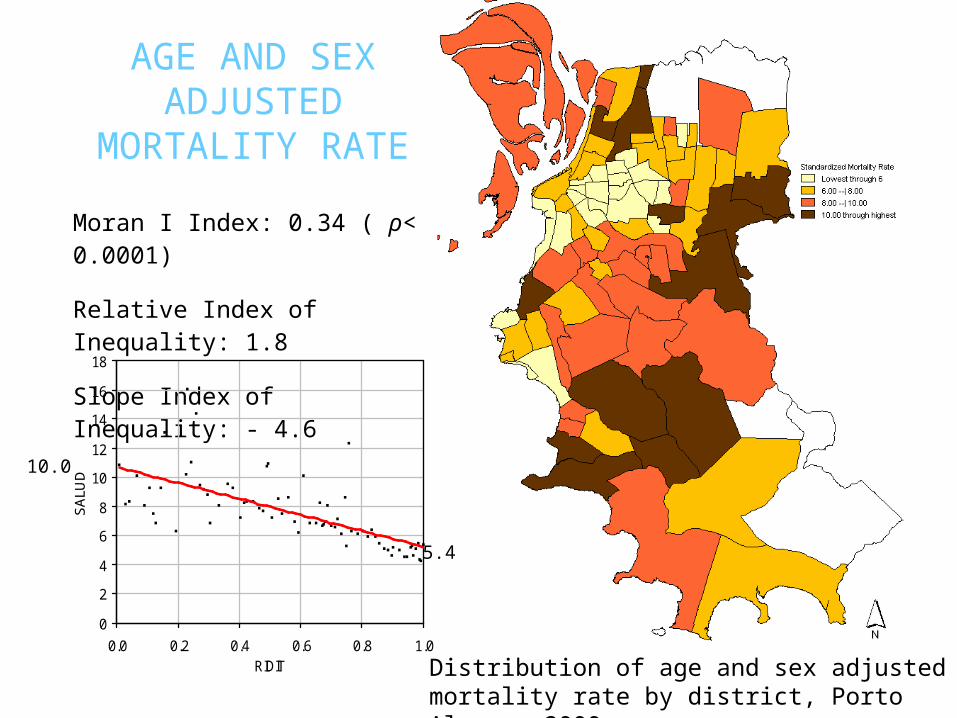
Distribution of age and sex adjusted mortality rate by district, Porto Alegre, 2000. Source: DATASUS-SIM

AGE AND SEX ADJUSTED

MORTALITY RATE

Moran I Index: 0.34 ( ρ< 0.0001)

Relative Index of Inequality: 1.8

Slope Index of Inequality: - 4.6

0

2

4

6

8

10

12

14

16

18

0.0 0.2 0.4 0.6 0.8 1.0RIDIT

SA

LUD

5.4

10.0

CARDIOVASCULAR DISEASES MORTALITY

45-64 YEARS CVD Deaths by 100,000

Distribution of age specific cardiovascular diseases mortality coefficient* , adjusted for age and sex, by district. Porto Alegre, 2000-2004. Sources: IBGE and SIM * results after smoothing

Moran I Index: 0.52 ( ρ< 0.0001)

Independent variablesDependent variables

Standardized B coefficients and (R2)

Income groups Isolation indexes

Total mortality

Premature CV

mortality

External causes

mortality

Pulmonary tuberculosis

incidence

Without income 0.28* (0.08) 0.26 * (0.07) 0.35* (0.12) 0.45** (0.20)

With income to < 2 ms 0.36 * (0.13) 0.37* (0.11) 0.42 ** (0.17) 0.52** (0.27)

2 to < 5 ms 0.19 (0.04) 0.18 (0.03) 0.22 (0.05) 0.30* (0.09)

5 to < 10 ms - 0.16 (0.03) - 0.19 (0.04) - 0.21 (0.04) - 0.13 (0.02)

10 to < 20 ms - 0.41** (0.17) - 0.44** (0.19) - 0.46** (0.21) - 0.37* (0.13)

20 or more ms - 0.53** (0.28) - 0.52** (0.27) - 0.53** (0.28) - 0.47** (0.22)

* Significant p<0.05** Significant p<0.001ms: minimum salaries/month Band Width: 400 m

Isolation indexes

Simple Linear Regression

Independent variablesDependent variables

Standardized B coefficients and (R2)

Income groups

Exposure indexes Total mortality

Premature CV

mortality

External causes

mortality

Pulmonary tuberculosis

incidence

>0 to <2 ms No income 0.31* (0.09) 0.29* (0.08) 0.38* (0.15) 0.49** (0.24)

2 to <5 ms < 2 ms 0.28* (0.08) 0.26* (0.07) 0.33* (0.11) 0.43** (0.19)

10 to <20 ms ≥ 20 ms - 0.52** (0.27) - 0.53** (0.28) - 0.54** (0.29) - 0.46** (0.21)

5 to <10 ms ≥ 10 ms - 0.41** (0.17) -0.44** (0.19) - 0.45** (0.21) - 0.36* (0.13)

* Significant p≤0.05** Significant p ≤ 0.001Band Width: 400 mSpearman Correlation Coefficient

Exposure indexes

Simple Linear RegressionTu

berc

ulos

is

Spatial Exposure Index>0 to <2 ms No income

2 to <5 ms < 2 ms 10 to <20 MS ≥ 20 ms 5 to <10 ms ≥ 10 ms

0.698** 0.679** -0.634** -0.488**

Average proportion of group n in the localities of each member of group m

Tube

rcul

osis

Tube

rcul

osis

Tube

rcul

osis

Independent variable

Dependent variables

Spatial CLUSTERING INDEX

Total mortality Premature CV mortality

External causes mortality

Pulmonary tuberculosis

incidence

Standardized B 0.65** 0.63** 0.64** 0.68**

R 2 0.42 0.39 0.41 0.46

Scattergram

** Significant p ≤ 0.01

CLUSTERING INDEX

Simple Linear Regression

Clustering Index Clustering IndexClustering IndexClustering Index

Dependent variablesStandardized B coefficients and R2

Independent variables Total mortality

Premature CV

mortality

External causes

mortality

Pulmonary tuberculosis

incidence

Mean Income - 0.40** - 0.30* - 0.31* - 0.33*

Clustering Index 0.33* 0.39* 0.41** 0.42**

R2 47.7 42.6 45.0 49,8

Mean Income - 0.54** - 0.46** - 0.47** - 0.59**

Isolation Index 10 or more ms

- 0.21 - 0.26* - 0.27* - 0.12

R2 46.5 41.5 43.8 44.1

Mean Income - 0.59** - 0.52** - 0.53** - 0.60**

Exposition Index 5 to <10 ms ≥ 10 ms

- 0.22* - 0.27* - 0.28** - 0.17

R2 48.0 43.3 46.0 45,6

* Significant p<0.05 ** Significant p<0.01 ms: minimum salaries/month

Linear Regression

Next steps:

Brazil: Obtain and analyse data for other Brazilian citiesIndia: Analyse DLHS-3 data in a multilevel and spatial context

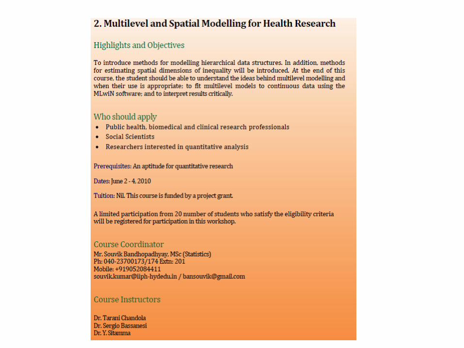
Workshops on Spatial and Multilevel Analysis:Brazil: May 18-20 2010India: June 2-4 2010