U.S. DEPARTMENT OF COMMERCE National Oceanic and Atmospheric Administration Air Resources Laboratory Special Operations and Research Division 232 Energy Way North Las Vegas, NV 89030

Telephone: (702) 295-1232 Fax: (702) 295-3068 Website: www.sord.nv.doe.gov

MEMO

November 17, 2010

Subject: Assessment of the Use of Speciated PM2.5 Mass-Calculated Light Extinction as a Secondary PM NAAQS Indicator of Visibility

From: Marc Pitchford, NOAA /s/

To: PM NAAQS Review Docket (EPA-HQ-OAR-2007-0492)

This memo documents the results of some of the assessment of the use of hourly PM2.5 mass concentration and relative humidity data and monthly-averaged PM2.5 composition to estimate daylight hourly-averaged PM2.5 light extinction (LE), based on the original IMPROVE algorithm. Hourly PM2.5 light extinction estimated in this manner is a contemplated indicator for a secondary PM national ambient air quality standard (NAAQS) to protect visibility. This memo addresses the effect of the monthly averaging aspect of this approach versus a day-by-day treatment. It also addresses the issue of whether certain features in the revised IMPROVE algorithm, where they differ from the original algorithm, should be incorporated into the speciated PM2.5 mass-calculated light extinction indicator. These features are (1) explicit treatment of “sea salt” in the approach, (2) site-specific values for Rayleigh light scattering, and (3) the use of the split component mass extinction efficiency approach. A more complete description of the original and revised IMPROVE algorithms is available in the literature.1

The Original IMPROVE Algorithm

The original IMPROVE algorithm for estimating light extinction (LE) is a simple linear equation that multiplies each of the concentrations of the major PM10 components by an extinction efficiency value to estimate its contribution to LE. The hygroscopic components (i.e., ammonium sulfate and ammonium nitrate) have extinction efficiencies that are dependent on the ambient relative humidity, while the other component extinction efficiencies are assumed to be constants. The sum of these terms is the estimate of the PM10 LE. The IMPROVE data managers routinely

1 Revised algorithm for estimating light extinction from IMPROVE particle speciation data. M. Pitchford et al., Journal of the Air Waste Management Association, 2007.

- 2 -

use 1-day-in-3 24-hour-averaged speciation data along with location-specific, monthly-averaged long-term (10 years) relative humidity (RH) values with the IMPROVE algorithm to generate daily visibility conditions needed to track visibility trends in federally protected remote areas as required for the Regional Haze Rule.2

More specifically, the original IMPROVE algorithm for estimating LE includes separate terms for five PM2.5 components, a term for PM10-2.5 mass, and a constant that accounts for Rayleigh light scattering by gaseous components of the atmosphere. When this algorithm is stripped of the PM10-2.5 and Rayleigh terms, it can be used to estimate PM2.5 LE in units of Mm-1 as shown in equation (1) below.

PM2.5 LE = 3f(RH) [AS] + 3f(RH) [AN] + 4[OM] + 10[EC] + 1[FS] (1)

where f(RH) is the relative humidity-dependent water growth function (i.e., the ratio of the hygroscopic fraction’s LE at ambient relative humidity to its LE when dry) and [AS], [AN], [OM], [EC] and [FS] are the concentrations in μg/m3 of ammonium sulfate, ammonium nitrate, organic matter, elemental carbon, and fine soil respectively. The water growth function is non-linear with a value 1.0 for relative humidity below 37% and up to ~4 at a relative humidity of 90%.3 The IMPROVE algorithm displayed as shown in equation (1) makes clear that the LE contributions by the various major component are separable. This is the basis for determining extinction budgets that have been widely used to approximately apportion LE to various PM2.5 components.

However, this five-factor algorithm for estimating hourly PM2.5 LE from hourly PM2.5 mass concentration and relative humidity data with auxiliary PM2.5 composition data can be expressed in a two-factor form by dividing both sides by PM2.5 mass and rearranging the terms into two extinction efficiency factors that depend on PM2.5 composition: one is the dry extinction efficiency and the other is the extinction efficiency increment due to the water content of the PM2.5 at ambient relative humidity. PM2.5 LE efficiency is the ratio of PM2.5 LE to the PM2.5 mass concentration, which in this case is the sum of the major PM2.5 components (i.e., [AS] + [AN] + [OM] + [EC] + [FS]), that when multiplied by the appropriately measured hourly PM2.5 mass will give PM2.5 LE. Rearranging the terms in equation (1) and dividing by the sum of the components yields the two terms that added together give extinction efficiency as shown in equation (2) below.

PM2.5 LE Efficiency = 3{(f(RH) -1)([AS] + [AN])} / ([AS] + [AN] + [OM] + [EC] + [FS]) +

(3[AS] + 3[AN] + 4[OM] + 10[EC] + 1[FS]) / ([AS] + [AN] + [OM] + [EC] + [FS]) (2)

2 40 CFR 51 subpart P.

3 Values for f(RH) are available at http://vista.cira.colostate.edu/improve/Tools/humidity_correction.htm.

- 3 -

The numerator of the first term, the extinction efficiency increment due to the water content of the ambient PM2.5 mass, is the product of a relative humidity function (i.e., 3(f(RH) – 1)) and the hygroscopic fraction (HF) of the PM2.5 components mass (i.e., HF = ([AS] + [AN])/([AS] + [AN] + [OM] + [EC] + [FS])). Division by the reconstructed PM2.5 mass makes the first term have units of light extinction efficiency. The second term in equation (2), the dry light extinction efficiency (DLEE), is the component concentration-weighted average of the individual dry component extinction coefficients (i.e., 3 for [AS] and [AN], 4 for [OM], 10 for [EC] and 1 for [FS]). PM2.5 LE efficiency in equation (2) can be rewritten in terms of the HF and DLEE as

PM2.5 LE Efficiency = 3((f(RH) -1)HF + DLEE (3)

where the first term is the extinction efficiency increment due to PM2.5-bound water that depends on PM2.5 composition and relative humidity, and the second term (DLEE) only depends on composition. With this form for expressing PM2.5 LE efficiency, equation (1) can be re-written as

PM2.5 LE = (PM2.5 mass) * [3((f(RH) -1)HF + DLEE] (4)

Both of the terms in the square brackets of equation (4) have a limited range of possible values within the constraints that we are interested in. The extinction efficiency water increment term ranges from zero, when either the relative humidity is below 37% or when HF = 0, to a maximum of about 9.5 m2/g for relative humidity at 90% and HF = 1 as shown in Figure 1. The uncertainty in the extinction efficiency water increment term caused by within-month variability of HF is assessed in the next section using 24-hour average concentration data. While the effect of relative humidity measurement uncertainty on the water growth term is not separately assessed, we can point out that the steep rise in the water growth function for high relative humidity conditions makes the case for taking and using accurate relative humidity measurements. The extinction efficiency water increment and its uncertainty are only of importance during periods with moderate to high relative humidity. As show in Figure 1, relative humidity must exceed ~50% for the extinction efficiency water increment to contribute at most 1 m2/g (for HF = 1) to the PM2.5 LE efficiency. The assessment described in the subsequent section shows the range and variability of the extinction efficiency water increment for a number of urban areas.

It should be noted that strictly speaking, equations (1) through (4) are algebraically consistent with one another only if PM2.5 mass in equation (4) is the sum of the mass of the five PM2.5 components used to derive the PM2.5 LE efficiency in equation (2) from the IMPROVE algorithm in equation (1). However, for the purposes of defining a PM2.5 light extinction indicator to be the basis for a secondary standard, another quantification of PM2.5 mass is anticipated in order to achieve hourly time resolution. Measurements of hourly time resolution for individual PM2.5 component mass are not practical or cost-effective. Also, while the sum of these components typically accounts for most of the dry PM2.5 mass in ambient air, especially in the remote rural environments for which the IMPROVE algorithm has been validated against

- 4 -

optical measurements, it will not necessarily be the same as the actual ambient PM2.5 mass that contributes to light extinction in urban areas, especially where road salt, sea salt, or industrial emissions with a different elemental mix than the "crustal" component in rural areas, may be present. (An assessment of the consequences of using PM2.5 mass for sites with significant contributions by PM2.5 sea salt is described below in this memorandum.) A gravimetric measurement of PM2.5 mass such as a measurement by the filter-based FRM, or by a continuous method well correlated to the FRM, would capture these other contributors to ambient PM2.5 mass, but may also result in reported mass values that include – as with the FRM -- some particle-bound water and/or that can have negative artifacts for ammonium nitrate under some conditions. Estimation of hourly PM2.5 mass on a day-specific and site-specific basis presumably must make use of data from on-site continuous PM2.5 instruments approved as FEM, in some way. Such data could be used directly, or normalized in some manner in an attempt to be more consistent with the sum of the five components. It remains to be investigated and considered what specific approach to using FEM data in equation (4) will work best in defining an indicator for hourly PM2.5 light extinction.

Figure 1. Water growth term from equation (3) which is the maximum water extinction efficiency for periods where the HF = 1.

The maximum range of DLEE is from 1, if all of the PM2.5 were fine soil, to 10 if all of the PM2.5 were elemental carbon. In urban areas, fine soil and elemental carbon tend to be the smallest two components of PM2.5 mass, which is typically dominated by some combination of ammonium sulfate, ammonium nitrate, and organic mass components. Since these have species extinction efficiencies of 3 m2/g, 3 m2/g, and 4 m2/g, the DLEE is generally near 3 m2/g to 4 m2/g. The

0

1

2

3

4

5

6

7

8

9

10

0 10 20 30 40 50 60 70 80 90 100

3*(f(

RH

) -1)

in u

nits

of m

2 /g

Relative Humidity (%)

Maximum Water Growth Term versus Relative Humidity

3*(f(RH) -1)

- 5 -

assessments described in the subsequent sections show the within-month variability for a number of urban areas of the HF and DLEE values, as well the performance of using monthly-averaged values in reproducing sample-day PM2.5 LE.

Performance Assessment for PM2.5 LE Using Monthly-Averaged Composition

“Performance” as used here refers to the degree of agreement between estimates of daily 24-hour PM2.5 light extinction efficiency based on monthly-average values of HF and DLEE with estimates of the same parameter based on same-day data. For simplicity, bounding values are assumed for relative humidity, rather than actual daily or hourly RH values from the four study areas.

One year (2008) of IMPROVE PM2.5 speciation data from four urban monitoring sites (Fresno, CA; Phoenix, AZ; New York, NY, and Washington, DC) were used to assess the ability of PM2.5 LE determined using monthly-averaged HF and DLEE to reproduce day-specific PM2.5 LE. Relative humidity data is not readily available at IMPROVE monitoring sites, so PM2.5 LE values were calculated for the two extremes of dry condition (i.e., RH < 37%) where only the DLEE is used, and moist conditions (i.e., RH ≈ 89.3%), where the maximum extinction coefficient water increment is 9 m2/g times the HF. Performance at any other relative humidity condition between these two extremes will be bounded by the performance at the two extremes.

The sample day-specific and monthly-averaged values of the maximum light extinction efficiency water increment, DLEE, and the sum of these that corresponds to the maximum total PM2.5 LE efficiency values for the four urban areas are shown as line plots in Figures 2, 3, 4, and 5. The time plots for the four urban areas show a greater day-to-day and seasonal variability in the maximum extinction efficiency water increment than for the DLEE. As anticipated, the DLEE tends to be in a range from 3 m2/g to 4 m2/g for each of the urban areas, though in Phoenix it drops to a value nearer to 2 m2/g in June due to higher relative contributions to PM2.5 by fine soil and to values somewhat higher than 4 m2/g in winter because of higher relative contributions by elemental carbon. The DLEE values for the other three urban areas have less seasonal variability.

- 6 -

Figure 2. Fresno monthly averaged and sample-day specific maximum extinction efficiency water increment (i.e., for RH≈89%) and dry light extinction efficiency (DLEE). Monthly averaged values are dashed lines. Red, blue, and black colored lines are for dry, wet, and total light extinction efficiency values respectively.

Figure 3. Phoenix monthly averaged and sample-day specific maximum extinction efficiency water increment (i.e., for RH≈89%) and dry light extinction efficiency (DLEE). Monthly averaged values are dashed lines. Red, blue, and black colored lines are for dry, wet, and total light extinction efficiency values respectively.

- 7 -

Figure 4. New York monthly averaged and sample-day specific maximum extinction efficiency water increment (i.e., for RH≈89%)and dry light extinction efficiency (DLEE). Monthly averaged values are dashed lines. Red, blue, and black colored lines are for dry, wet, and total light extinction efficiency values respectively.

Figure 5. Washington monthly averaged and sample-day specific maximum extinction efficiency water increment (i.e., for RH≈89%)and dry light extinction efficiency (DLEE). Monthly averaged values are dashed lines. Red, blue, and black colored lines are for dry, wet, and total light extinction efficiency values respectively.

- 8 -

Table 1 shows the coefficient of variation (i.e., standard deviation divided by the mean times 100%) for the DLEE and maximum extinction efficiency water increment values by month, the mean of the 12 monthly values, and the annual values. These give a more quantitative view of the variability patterns seen in Figures 2 through 5. The within-month variabilities of the dry extinction efficiency values are generally less than about 10%, except at Phoenix during a few months when the coefficient of variation is nearer 20%, due to periods where the day-specific values are low because of higher relative contributions to PM2.5 by fine soil. The within-month variabilities of the maximum extinction efficiency water increment are generally less than 15% except for a few months at Fresno where the coefficient of variation is closer to 20%, due to large within-month variations in the HF during the winter months. The San Joaquin Valley where Fresno is located is known to experience episodes of high nitrate concentrations in cooler months. The means of the monthly extinction efficiency water increment coefficient of variation values are significantly lower than the annual values, while the mean monthly DLEE coefficient of variation values are more comparable to the annual values. This indicates that the use of monthly-averaged values is important to account for seasonal patterns in the maximum extinction efficiency water increment, while annual-averaged DLEE would perform almost as well as monthly averaged values.

Table 1. Monthly and annual coefficient of variation (%) for the dry and maximum water extinction coefficients for four urban areas.

   

Fresno Phoenix  New York  Washington 

Dry Water Dry Water Dry Water Dry Water

January 10.8 17.1 4.9 13.5 6.1 5.5 4.2 6.8

February  7.9 16.2 6.9 10.4 10.1 5.7 3.7 7.7

March 9.1 10.4 10.3 5.8 6.2 9.7 3.1 5.6

April 4.2 11.2 12.8 5.7 4.6 9.0 5.4 12.7

May 13.1 14.2 21.1 12.4 9.5 13.3 6.9 6.8

June 9.2 12.6 26.7 10.0 4.0 8.7 6.1 10.6

July 5.3 8.0 7.3 3.8 10.0 11.9 5.9 7.3

August 6.8 6.1 8.4 8.4 7.3 10.6 4.7 7.8

September 4.8 7.3 11.2 13.2 5.9 8.2 4.3 5.7

October 9.3 8.7 10.7 4.2 6.8 8.9 5.4 10.0

November 5.8 12.1 18.1 6.2 6.7 8.4 1.7 7.7

December 8.7 20.9 5.4 8.1 7.2 5.5 4.9 6.1

Mean Monthly  7.9 12.1 12.0 8.5 7.0 8.8 4.7 7.9

Annual 10.2 38.7 18.4 40.5 7.7 19.8 5.7 17.4

- 9 -

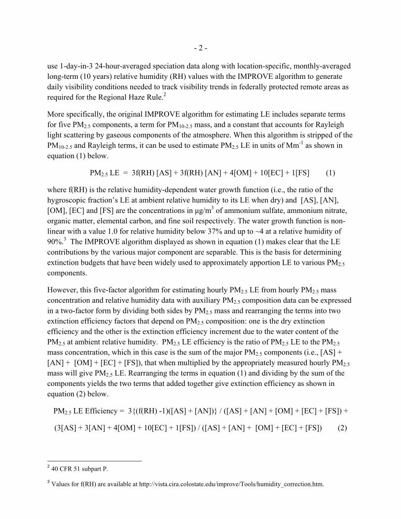
Figures 6, 7, 8, and 9 are paired scatter plots of PM2.5 LE calculated using monthly-averaged PM2.5 LE efficiencies versus those calculated using sample-day specific PM2.5 LE efficiencies for dry and moist conditions. In all cases, the sum of the day-specific PM2.5 component concentrations were used as the PM2.5 mass concentration that was multiplied by the extinction efficiency values to calculate PM2.5 LE. The simple linear regression equation and the R2 values (i.e., the fraction of the variance explained, where R2 = 1.0 is a perfect fit) for each are shown on the plots. The scatter plots and regression fits for each site indicate a strong correlation between the PM2.5 LE calculated using monthly mean composition values with day-specific PM2.5 LE. The performance is somewhat better when relative humidity is assumed to be low compared to when it is assumed to be high. Among these four urban areas, the fit for Phoenix is the worst with R2 = 0.93 for assumed dry conditions and 0.87 for the high humidity condition case. The relationship using actual relative humidity conditions will be bounded by these two extremes, so for the generally dry conditions in Phoenix using ambient relative humidity should result in a relationship closer to the dry extreme R2 value. The R2 values for the other three urban areas range from 0.96 to 0.98.

Apparent from the Figures 6 through 9 is that for each urban location the PM2.5 LE values range over a factor of about 10. This corresponds well to the range of 24-hour PM2.5 mass concentration values for these urban areas, with their range of about a factor of 10. Though not explicitly evaluated in this assessment, the role of relative humidity conditions in the calculation of light extinction can be appreciated by noting the doubling or more of the axis scales for the scatter plots displaying the highest humidity cases compared with the corresponding axis scales for dry case scatter plots in Figures 6 through 9. This implies that variations in relative humidity alone can change the water content of PM2.5 in these urban enough to result in as much as a factor of two range in PM2.5 LE values. Based on these observations and the fact that PM2.5 LE determined using monthly averaged composition (i.e., HF and DLEE values) does not much differ from PM2.5 LE values calculated with day-specific composition, it would appear that the most influential factors that influence variability of PM2.5 LE are PM2.5 mass, followed by relative humidity, with composition being the least important so long as monthly-averaged HF and DLEE are used in the calculation, rather than any longer-term average values. Use of monthly-averaged values for each site seems to sufficiently capture the seasonal and regional differences in the relationship between PM2.5 LE and measured PM2.5 mass and relative humidity data. The largest differences caused by using monthly-mean composition percentages instead of day-specific percentages are for Fresno under conditions of high relative humidity and high PM2.5 concentrations. This is consistent with the known occurrence of high nitrate concentrations on some but not all days during cool months. The use of monthly averages underestimates HF (and hence the light extinction) on days with the highest nitrate concentrations and overestimates it on other days.

- 10 -

Figure 6. Scatter plots of monthly averaged composition calculated PM2.5 LE versus day specific composition calculated light extinction for dry (top) and high humidity (bottom) conditions, using Fresno 2008 data.

- 11 -

Figure 7. Scatter plots of monthly averaged composition calculated PM2.5 LE versus day specific composition calculated light extinction for dry (top) and high humidity (bottom) conditions, using Phoenix 2008 data.

- 12 -

Figure 8. Scatter plots of monthly averaged composition calculated PM2.5 LE versus day specific composition calculated light extinction for dry (top) and high humidity (bottom) conditions, using New York 2008 data.

- 13 -

Figure 9. Scatter plots of monthly averaged composition calculated PM2.5 LE versus day specific composition calculated light extinction for dry (top) and high humidity (bottom) conditions, using Washington 2008 data.

Sea Salt Assessment

- 14 -

The original IMPROVE equation has been revised to include sea salt contributions, which can be significant at some coastal locations and contribute significantly to remote area visibility conditions that are of concern for the Regional Haze Rule.4 A sea salt term could be added to the algorithm shown above for extinction efficiency (equation 3). Because sea salt has a significantly different water growth curve than that used for AS and AN, a version of equation (4) that included sea salt explicitly would be a three-factor instead of two-factor algorithm. The question at issue here is whether sea salt should be explicitly included in the calculation of light extinction.

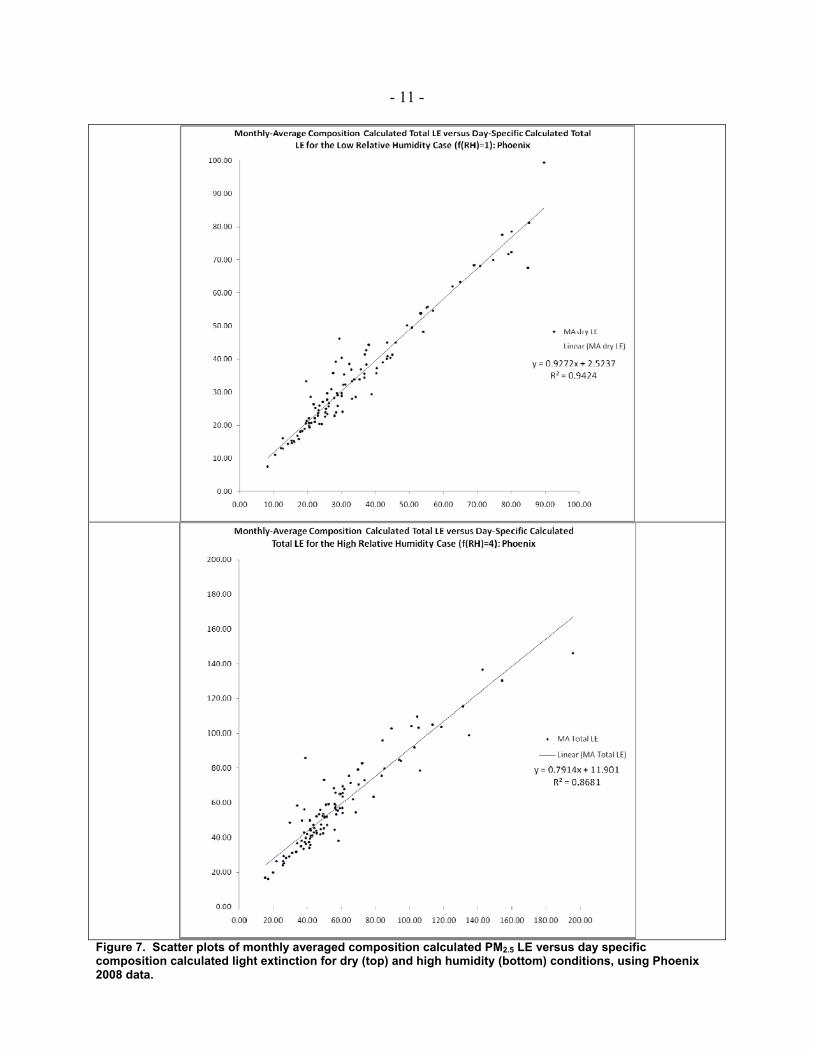
To examine this question, data from the Chemical Speciation Network (2000 to 2008) for ten monitoring sites (see Table 2) with high annual sea salt concentrations were used to calculate the sea salt contribution to PM2.5 LE. Sea salt concentration and contribution to PM2.5 LE were based on the chlorine concentration using the method in the revised IMPROVE algorithm. Day-specific relative humidity data for these sites were not readily available so the long-term monthly mean relative humidity conditions as used in Regional Haze Rule calculations were used for each sampling day in a month in place of day-specific data.

Table 2 Site codes and locations for sites with high annual sea salt concentrations.

AQS Site ID Location AQS Site ID Location

530530029 Tacoma, WA 150032004 Pearl City, HI

530330080 Seattle, WA 121030026 Tampa, FL

482011039 Houston, TX 120573002 Central Florida

410390060 Eugene, OR 120111002 Miami, FL

330150014 Portsmouth, NH 060850005 San Jose, CA

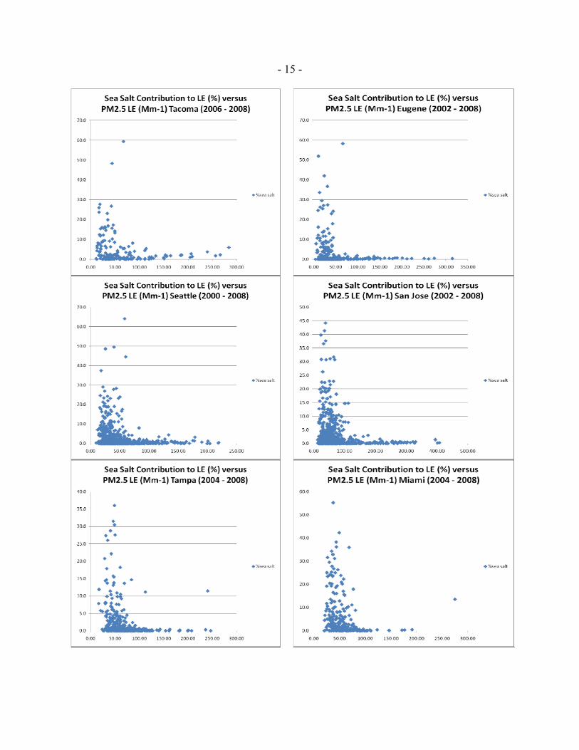
Figure 10 contains scatter plots of the percent contributions by sea salt to 24-hour PM2.5 LE versus the 24-hour PM2.5 LE level for each of the ten sites. As seen in these figures, sea salt can contribute substantially (i.e., >25%) to PM2.5 LE on days with low to moderate PM2.5 LE levels. However except for a few outliers, the contributions to PM2.5 LE are well below 5% for PM2.5 LE greater than 100 Mm-1. From these plots it would seem that not explicitly including a sea salt term in the calculated PM2.5 LE does not have an important effect on LE estimates on days that would likely exceed a new secondary NAAQS, even for locations that have the greatest average concentrations of PM2.5 sea salt.

4 Pitchford M; Maim W; Schichtel B; Kumar N; Lowenthal D; Hand J (2007). Revised algorithm for estimating light extinction from IMPROVE particle speciation data. J Air Waste Manag Assoc, 57: 1326-36.

- 15 -

- 16 -

Figure 10. Percent contributions to PM2.5 LE by sea salt versus PM2.5 LE levels for ten CSN monitoring sites with the highest annual sea salt concentrations.

It should be noted that not explicitly including a sea salt term in the calculation of the water extinction efficiency and DLEE does not mean that the contributions of sea salt are entirely excluded in the calculated PM2.5 LE, if the measured hourly PM2.5 mass concentration that includes the mass of the sea salt is used directly in equation (4). In other words, the additional PM2.5 mass from sea salt is transformed into PM2.5 LE using the extinction efficiency values calculated from monthly–averaged non-sea salt PM2.5 component composition and relative humidity. A logical question is how much uncertainty and/or bias in PM2.5 LE does this contribute.

To assess the effect of calculating PM2.5 LE using extinction efficiencies that do not explicitly include a sea salt term, but have a substantial contribution by sea salt to the PM2.5 mass, a sensitivity analysis was conducted using hypothetical data over a range of conditions. Three hypothetical PM2.5 compositions were assumed (i.e., low, medium, and high non-sea salt HF values of 0.2, 0.5, and 0.7 respectively), each with PM2.5 mass = 50 μg/m3 of which 10 μg/m3 is

- 17 -

sea salt, and a DLEE value for the non-sea salt components of 4 m2/g. PM2.5 LE levels were calculated for each of these for six relative humidity values (i.e., RH = 40%, 50%, 60%, 70%, 80%, and 90%) using two different approaches. One of the two approaches (shown as LEoriginal) multiplies the PM2.5 mass (i.e., 50 μg/m3) times PM2.5 LE efficiency from equation 3 that does not include sea salt explicitly and where the extinction efficiency is calculated using the five-component reconstructed mass. The other approach (LErevised) is calculated using the algorithm with the sea salt term and water growth functions from the revised IMPROVE algorithm. All other aspects for the two approaches are identical (e.g., same dry species extinction efficiencies). The results of these calculations are shown in Figure 11 as plots of PM2.5 LE by both methods as a function of relative humidity for each of the three non-sea salt HF component levels.

The two algorithms give broadly similar results with the greatest absolute differences for the case with low non-sea salt HF when the relative humidity is at or below 40% and at 90%. The average fractional differences across the six relative humidity values are 0.4%, 4.9%, and 6.7% for the low, medium, and high non-sea salt HF cases respectively, with the greatest fractional errors at RH=40% where the original algorithm approach overestimates PM2.5 LE by about 13% for each of the HF cases.

- 18 -

Figure 11. PM2.5 LE calculated using the original IMPROVE algorithm without an explicit sea salt term and using the sea salt term from the revised IMPROVE algorithm versus relative humidity for three HF conditions, HF = 0.2 (top), HF = 0.5 (middle), and HF = 0.7 (bottom). PM10 and sea salt concentrations set at 50 μg/m3 and 10 μg/m3 respectively for all calculations.

- 19 -

Rayleigh Light Scattering

The revised IMPROVE algorithm includes the use of standardized site-specific Rayleigh scattering values rounded to the nearest integer Mm-1 (revised algorithm), while 10 Mm-1 is used for all sites in the original IMPROVE algorithm. The standardized site-specific Rayleigh values depend on the typical density of the atmosphere which is primarily a function of elevation and temperature. The resulting values range from about 8 Mm-1 at about 4 km elevation to about 12 Mm-1 at sea level. The calculation of PM2.5 LE does not include a Rayleigh term, however 10 Mm-1 was subtracted from the LE values that corresponded to the 20 dv to 30 dv range from the preference studied (UFVA Chapter 2) used to define the CPL. The maximum difference between the two approaches for treating Rayleigh scattering is 2 Mm-1.

Split Component Mass Extinction Efficiency

The most significant difference between the original and refined IMPROVE algorithm is the use of a more complex approach in the revised algorithm to account for biases between direct measurements of light scattering and original algorithm estimates of light scattering extinction. These biases are largest at the low and high ends of the range of light extinction for remote areas monitoring sites. In essence, the original algorithm’s set of dry extinction efficiency values for the major species were selected to work well across the range of conditions in available data sets. While the original IMPROVE algorithm is successful for most conditions, for the lowest PM concentration conditions it tends to overestimate the PM LE, while for the highest PM concentrations it tends to underestimate the PM LE. The best explanation for this behavior is that the size distribution and hence the dry light extinction efficiency of ambient particles tend to be smaller when the concentrations are low and larger when the concentrations are larger. How much of this behavior is due to differences in particle formation mechanisms or the result of aging of the particles is unclear. It is also unclear whether this behavior applies in urban areas, where more of the ambient PM is attributable to recent or “fresh” local emissions, compared to remote areas farther from emission sources.

The revised algorithm uses a so-called “split component mass extinction efficiency model” to account for this tendency for lower dry extinction efficiencies at low concentrations and higher dry extinction efficiencies at high concentrations. Three species, ammonium sulfate, ammonium nitrate, and organic mass compounds (i.e., AS, AN, OMC) are each assumed to be a mixture of two extreme particle size distributions, one labeled “small” and the other “large”. The extinction efficiencies were determined based on typical measured small and large size distributions, so that the extremes would be anchored to realistic ambient particle properties. The relative concentrations of the small and large particle distributions of each species was determined empirically using a simple linear relationship to species concentrations that provided an improved correspondence between nephelometer-measured and algorithm-estimated light scattering at 21 monitoring sites in remote areas.

- 20 -

The revised algorithm light extinction terms for ammonium sulfate, ammonium nitrate, and organic mass components are as follows

LEAS ≈ 2.2 x fs(RH) x [ASs] + 4.8 x fL(RH) x [ASL] (4)

LEAN ≈ 2.4 x fs(RH) x [ANs] + 5.1 x fL(RH) x [AN] (5)

LEOMC ≈ 2.8 x [OMCs] + 6.1 x [OMCL] (6)

where subscripts S and L denote small and large particle size distributions for the three components and for the water growth functions of relative humidity. The concentrations of the large particle size distributions for each species is set equal to the ratio of its total concentration divided by 20 μg/m3 times the total concentration of the species, and the concentration of the small particle size distribution is the difference between the total concentration of the species and the concentration of the large size distribution. For example if [OMC] = 4 μg/m3, then [OMCL] = 4/20 x 4 μg/m3 or 0.8 μg/m3 and [OMCs] = 4 μg/m3 – 0.8 μg/m3 or 3.2 μg/m3. If the concentration of one of the species exceeds 20 μg/m3 then all of that species concentration is assumed to be in the large particle size distribution.

As is contemplated using the original IMPROVE algorithm, the revised IMPROVE algorithm could be used to estimate hourly PM2.5 LE by employing the same assumption that the monthly mean relative PM2.5 composition adds little uncertainty when applied to hourly PM2.5 mass concentration and relative humidity data. It does, however, add to the complexity of the computations, since the concentrations and resulting extinction efficiencies of the large and small particle size distributions need to be determined for each of the three split species for each hour. For the two-factor version of the original IMPROVE algorithm as shown in equation (4), the algorithm can be reformulated so that a pair of monthly-averaged terms (i.e., HF and DLEE) would be all that is needed to determine hourly PM2.5 LE from hourly PM2.5 concentration and relative humidity data for each monitoring site. In contrast, if the split component approach were used, each hour would require calculations using the five monthly-averaged composition percentages to apportion the hourly PM2.5 mass concentrations into the five components, followed by apportion of the AS, AN, and OMC components into large and small size distribution split species, followed by the calculation of hourly PM2.5 LE. This process could be incorporated into a software program so the routine burden for those responsible for making the calculation would be minimal, though it would be more complicated than use of the original algorithm approach formulated in equation (4).

The magnitude of the difference between LE calculated using the revised and original IMPROVE algorithms is demonstrated in Figure 12 using 2004 24-hour data from two urban IMPROVE monitoring sites (Phoenix and Washington). These are data taken from the VIEWS website. LE is calculated using the 10-year averaged monthly relative humidity growth factors and different assumed OMC to OC ratios (1.4 for the original and 1.8 for the revised algorithms respectively). As can be seen in the plots, the revised and original algorithm calculations diverge little from the 1-to-1 line for days with LE up to about 50 Mm-1 but by 200 Mm-1 using the

- 21 -

original algorithm, the revised algorithm estimated LE is about 250 Mm-1. From the power law regression equation fits and R2 values shown for the two urban areas, the site-specific relationships between the revised and original algorithm are strong, but differ for the two urban areas. Analysis of results from other locations can be expected to demonstrate similar differences at high LE values as seen in this assessment.

Figure 12 Scatter plot of LE estimates from the revised (y-axis) versus the original (x-axis) IMPROVE algorithms for Washington (blue) and Phoenix (red) based on 2004 IMPROVE data downloaded from the VIEWS website. The power law regression lines, equations and R2 values for the two data sets are shown as is a 1 to 1 line.

The revised IMPROVE algorithm was developed using data from remote area locations with collocated nephelometers. There is only limited urban data available upon which to check its applicability. In comments received on the second draft PAD from UARG, an assessment using

- 22 -

data from the Atlanta, GA SEARCH site showed that the revised algorithm with the split component mass extinction efficiency and a OMC to OC ratio of 1.8 performed better at predicting nephelometer-measured light scattering than the original algorithm using either 1.4 or 1.8 for the OMC to OC ratio.5 The results of this one-site assessment suggest that the LE estimates from the revised IMPROVE algorithm may be more appropriate for Atlanta than estimates from the original algorithm.

Summary and Conclusions

The original IMPROVE algorithm can be reformulated to calculate PM2.5 LE by multiplying PM2.5 mass times a term that depends on particle composition and relative humidity. PM2.5 LE efficiency is the sum of two factors. The first is the water extinction efficiency which is the product of the hygroscopic fraction (HF) and a function of relative humidity that accounts for the PM2.5-bound water at any elevated humidity level. The second term is the dry light extinction efficiency (DLEE) which is a component concentration-weighted average of the individual component extinction efficiencies (i.e., 3 m2/g for ammonium sulfate and nitrate, 4 m2/g for organic mass, 10 m2/g for elemental carbon, and 1 m2/g for fine soil). While HF and DLEE vary when the composition of the PM2.5 changes, they are bound by the constraints of their definition (i.e., 0 < HF < 1, and 1 m2/g < DLEE < 10 m2/g) and tend to be sufficiently well behaved that monthly-averaged values of both can be combined with day-specific 24-hour PM2.5 mass and bounding values for relative humidity to generate 24-hour PM2.5 LE values that agree quite well with 24-hour PM2.5 LE values using day-specific composition and the same bounding values of relative humidity. Though not explicitly demonstrated here, this good performance using monthly-averaged HF and DLEE should transfer to the estimation of hourly PM2.5 LE when combined with hourly PM2.5 mass concentration and hourly relative humidity data.6

Contributions to PM2.5 LE by sea salt at the coastal areas where it might be important were examined several ways. Assessment of sea salt’s contribution to PM2.5 LE at 10 CSN monitoring sites with high annual sea salt contributions were shown to be minor for high haze levels (i.e., sea salt PM2.5 LE < 5% when total PM2.5 LE > 100 Mm-1). The IMPROVE algorithm can be modified to explicitly include sea salt by adding an additional water growth curve and using calculated sea salt mass from PM2.5 chlorine concentration. A sensitivity assessment showed that use of the original algorithm without an explicit sea salt term performs well at estimating PM2.5 LE over a range of composition and relative humidity conditions. Given the small influence of sea salt at the likely NAAQS control levels, that it is emitted from a natural process (i.e., spray

5 Comments of the Utility Air Regulatory Group on Chapter 4 of the Policy Assessment for the Review of the Particulate Matter National Ambient Air Quality Standards – Second External Review Draft (June 2010), Attachment A, August 30, 2010.

6 Appendix F of the final Policy Assessment Document examines the results of using hourly relative humidity data instead of bounding values. It also compares an approach (“approach T”) that uses monthly-averaged composition to an approach (“approach W”) that uses only same-day composition.

- 23 -

and breaking waves), and the ability of the simpler algorithm to adequately calculate PM2.5 LE for cases with high sea salt, there seems to be little reason to employ the more complicated algorithm that explicitly includes a sea salt term.

The maximum difference between the two approaches for treating Rayleigh light scattering (i.e., site-specific or constant = 10 Mm-1) is 2 Mm-1, which is only a few percent of the values being considered for the protection level of the standard, so accounting for it is not thought to warrant the extra complication of having different values for different locations.

The simplicity of the single species extinction efficiency of the original IMPROVE algorithm compared to the split component mass extinction efficiency approach used in the revised algorithm is an attractive feature. The difference between the two approaches is only significant at the higher PM2.5 LE levels where the revised algorithm approach would estimate larger values than those from the original algorithm. Given the limitations of available directly measured PM2.5 LE in urban areas upon which to base a choice between the two approaches, EPA should pursue the simpler approach, but also solicit comments on the appropriateness of using the revised algorithm in place of the original algorithm as the basis for the speciated PM2.5 mass-calculated LE indicator.