u.s. gaap & ifrs: today and tomorrow sept. 13-14, 2010 · pdf fileu.s. gaap & ifrs:...

U.S. GAAP & IFRS: Today and Tomorrow Sept. 13-14, 2010

New York

Variable Annuities

Patricia Matson

1

GAAP for Variable andGAAP for Variable and Fixed Annuities

Tricia Matson, Principal, Deloitte Consulting LLP

Agenda

• Introduction to FAS 133• Variable Annuity Topics

Embedded derivatives in variable annuities– Embedded derivatives in variable annuities• Identification• Accounting ramifications

– Accounting for various features under SOP 03-1– Summary of accounting for different benefit types– DAC topics

• Fixed Annuity Topics

1

– FAS 133 for EIAs

2

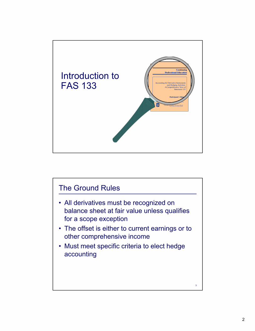
Introduction toContinuing

Professional EducationContinuing

Professional EducationIntroduction to FAS 133

Accounting for Derivative Instrumentsand HedgingActivities:

AComprehensive ViewofStatement 133

Participant's Manual

FinancialAccounting Standards Boardofthe Financial Accounting Foundation

Accounting for Derivative Instrumentsand Hedging Activities:

AComprehensive View ofStatement 133

Participant's Manual

The Ground Rules

• All derivatives must be recognized on balance sheet at fair value unless qualifies for a scope exception

• The offset is either to current earnings or to other comprehensive income

• Must meet specific criteria to elect hedge accounting

3

accounting

3

Why is FAS133 so Complex?

• Derivatives are complex• “Cover all bases” approach in definingCover all bases approach in defining

“derivative”• Accommodate hedge accounting to deal

with anomalies caused by mixed-attribute model

4

FAS 133: The Big Picture

• In summary:– Broadly defines a derivativey– Introduces concept of embedded derivatives– All derivatives at fair value on the balance

sheet (previously off balance sheet)– Default accounting – MTM in earnings

Limited hedge accounting permitted

5

– Limited hedge accounting permitted

4

FASB’s Definition of a Derivative

Any contract with ALL of the following:1. Financial instrument or contract

FAS 149 amended –less than 90% of

ti l- Underlying- Notional amount or payment provision

2. No (or smaller) investment at inception3. Requires or permits net settlement or de facto net

settlement

notional

6

Definition of Derivative

Examples of Notionals and Underlyings:Derivative Underlying Notional

FAS 149 – include occurrence /

nonoccurrence of specified events

Stock option Stock price Number of shares

Currency forward Exchange rate Amount of currency

Commodity future Commodity price Number of commodity units

7

Interest rate swap Interest rate index Dollar amount

Purchase order computers

Price of computers Number of computers

5

Net Settlement

1. Neither party must deliver the underlying asset and the contract settles on a net basis

N t h h ttl tNet cash or share settlement2. One party must deliver the underlying asset, but

- there is a mechanism that facilitates net settlement (e.g. exchange, assignment)

– or –the asset is readily convertible to cash or is itself a

8

- the asset is readily convertible to cash or is itself a derivative (e.g. publicly traded securities would be readily convertible to cash)

Identifying Embedded Derivatives

9

6

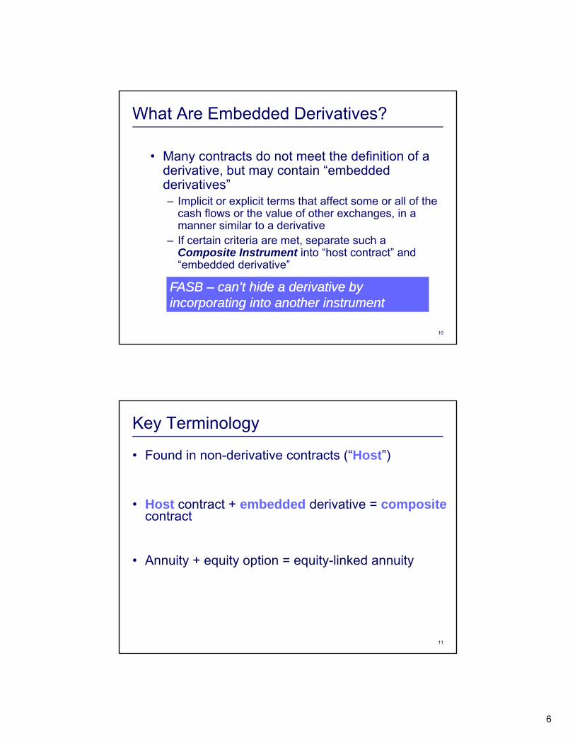
What Are Embedded Derivatives?

• Many contracts do not meet the definition of a derivative, but may contain “embedded , yderivatives”– Implicit or explicit terms that affect some or all of the

cash flows or the value of other exchanges, in a manner similar to a derivative

– If certain criteria are met, separate such a Composite Instrument into “host contract” and

10

“embedded derivative”

FASB FASB –– can’t hide a derivative by can’t hide a derivative by incorporating into another instrumentincorporating into another instrument

Key Terminology

• Found in non-derivative contracts (“Host”)

• Host contract + embedded derivative = compositecontract

• Annuity + equity option = equity-linked annuity

11

7

> Convertible debt – Generally bifurcate embedded derivative

Composite Instruments

> Calls and puts on equity instruments– Bifurcate embedded derivative

> Equity-indexed note– Bifurcate embedded derivative

12

Host

Embedded Derivatives Decision Tree

KEYKEY

Is contract already marked to fairvalue through

earnings?

Does the embedded

meet the definition of a derivative?

Is it clearly and Is it clearly and closely relatedclosely related

to the host?to the host?

No Yes No

Yes No Y

13

Yes No Yes

Do Not Apply Statement 133Do Not Apply Statement 133

8

What is Clearly and Closely Related?

Cl l d l l l t d f t• Clearly and closely related refers to:– Economic characteristics– Risks– Defined mostly by examples in FAS 133

• Factors to consider

14

– Type of host– Underlying

Life Insurance and Annuities

> Excluded from FAS 133:

– Traditional whole-life contracts (FAS 60)Out– Traditional participating contracts (FAS

120/SOP 95-1)– Traditional universal-life contracts (FAS 97)

> Generally Subject to FAS 133 (depends on facts & circumstances):

– Deferred variable annuity with a minimum guaranteed investment returnIn

15

– Equity-indexed deferred annuity and life insurance

– Synthetic GICs– GMAB/WB– GMIB, if net settled– Certain reinsurance agreements

9

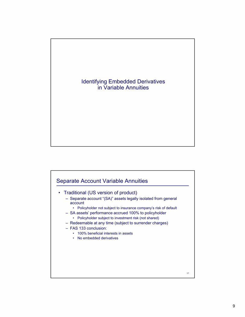
Identifying Embedded Derivativesin Variable Annuities

Separate Account Variable Annuities

• Traditional (US version of product)– Separate account “(SA)” assets legally isolated from general

account• Policyholder not subject to insurance company’s risk of default

– SA assets’ performance accrued 100% to policyholder• Policyholder subject to investment risk (not shared)

– Redeemable at any time (subject to surrender charges) – FAS 133 conclusion:

• 100% beneficial interests in assets• No embedded derivatives

17

10

Separate Account Variable Annuities

• Non-traditional features– Most features are not clearly and closely related, because they

result in sharing of investment riskg– However, many such features do not meet the definition of

derivative

18

Guaranteed Minimum Death Benefits

• Host contract– Annuity

• Embedded derivativeEmbedded derivative– Option

• Clearly and closely related?– No!– Embedded derivative scoped out as

insurance

19

11

Guaranteed Minimum Accumulation Benefits

• Separate account A issues variable annuity for $1 million. • Separate account guarantees a minimum account value

of $1 million at end of guarantee periodof $1 million at end of guarantee period. • If policyholder terminates before end of accumulation

period, the policyholder will receive the account value less surrender charges.

20

Guaranteed Minimum Accumulation Benefits


• Embedded derivative– Option

• Clearly and closely related?– No!– Sharing of investment risk

21

12

Guaranteed Minimum Withdrawal Benefits

• Separate account A issues variable annuity for $1 million.• Variable annuity contains a GMWB. • GMWB guarantees $1 million value through fixed payouts• GMWB guarantees $1 million value through fixed payouts

that do not exceed $70,000 per year. (This is equivalent to a guarantee of about 14 years.)

22

Guaranteed Minimum Withdrawal Benefits



• Clearly and closely related?– No!– Sharing of investment risk

23

13

GMWB for Life

• Separate account A issues variable annuity for $1 million. • Variable annuity contains a GMWB for Life. • GMWB guarantees $1 million value through fixed payouts• GMWB guarantees $1 million value through fixed payouts

that commence at age 65 and do not exceed $5,000 per year, payable for life.

24

GMWB for Life (for Life Component)



• Clearly and closely related?– No!– Sharing of investment risk– View A - Life contingent portion

scoped out as insurance– View B – Conversion of contract

25

– View B – Conversion of contract to life annuity when account value is zero constitutes a net settlement of derivative; therefore, not scoped out.

14

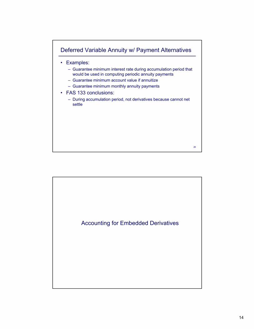
Deferred Variable Annuity w/ Payment Alternatives

• Examples:– Guarantee minimum interest rate during accumulation period that

would be used in computing periodic annuity payments– Guarantee minimum account value if annuitize– Guarantee minimum monthly annuity payments

• FAS 133 conclusions:– During accumulation period, not derivatives because cannot net

settle

26

Accounting for Embedded Derivatives

15

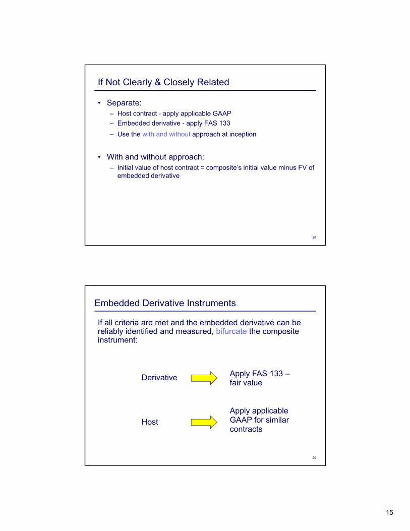
If Not Clearly & Closely Related

• Separate:– Host contract - apply applicable GAAP – Embedded derivative - apply FAS 133Embedded derivative apply FAS 133 – Use the with and without approach at inception

• With and without approach:– Initial value of host contract = composite’s initial value minus FV of

embedded derivative

28

Embedded Derivative Instruments

If all criteria are met and the embedded derivative can be reliably identified and measured, bifurcate the composite instrument:

Apply FAS 133 –fair valueDerivative

29

Apply applicable GAAP for similar contracts

Host

16

Can’t Bifurcate?

If the embedded derivative cannot be reliably measured:– Account for entire contract at fair value through earnings

Composite may not be used as a hedging instrument– Composite may not be used as a hedging instrument– Should be rare

30

What is “Fair Value”?

– FAS 133 indicates use of “fair value”

– FAS 157 establishes definition

– FAS 157 will be discussed in “Fair Value” presentation

31

17

FAS 133 Valuation of GMWBCommon Practices Before FAS 157

• Risk neutral stochastic models• Liability = expected (PV benefit + PV risk margins - PV fees)• Pre-157 common practicesp

– Discount using risk-free rates or swap rates– Update assumptions, in force, stochastic model parameters– Assume “risk margin” at issue such that FV of embedded derivative

was zero; not many insurers unlocked risk margins in practice (many used “attributed fee” approach)

– No direct recognition for non-performance risk

32

FAS 133 Valuation of GMWB Valuation Considerations– Modeling

• Need relatively granular model in order to minimize offsetting effect of different levels of in-the-moneyness

• Careful consideration should be given to the interplay of various guaranteesg p y g• Number of scenarios must be sufficient

– Assumptions• Economic – fund growth, volatility• Non-economic - mortality, persistency (including dynamic lapse), benefit

utilization (varies depending on in-the-moneyness); “static” assumptions generally consistent with DAC assumptions

– Changes in value of embedded derivative should flow through EGPs

33

g g(along with earnings on assets backing embedded derivatives)

– Importance of controls – model risk substantial, as small changes to models can have a large impact

18

Application of SOP 03-1 to Variable Annuities

Separate Account ConsiderationsSeparate Account Criteria

• “The portion of separate account assets representing contract holder funds should be measured at fair value and reported in the insurance enterprise’s financial statements as a summary total, with an equivalent summary total for related liabilities”

• Must meet four criteria in ¶ 11– Separate Account legally recognized– Separate Account assets legally insulated from General Account

liabilities– Allocations of Separate Account funds directed by the contract holder

35

p y– Investment performance passed through to the contract holder (net of

fees and assessments)

19

Separate Account ConsiderationsAccounting Implications• Some VA-like products (e.g., MVAs, UK Unit-linked) are not

eligible for Separate Account treatment• Reserves for minimum guarantees are held in general g g

account • Insurer seed money is reclassified as General Account

asset• Assets transferred between General Account and Separate

Account may create gains or losses

36

Valuation of LiabilitiesDetermining Significance of Mortality / Morbidity Risk

• Contracts classified either as “Universal Life type” or “Investment” contracts; no additional liability allowed for investment contractsinvestment contracts

• Significance determined at contract inception (other than transition)

• Compare PV of excess benefit payments to PV of contract holder assessments

• In performing the analysis, consider both frequency and it d f ll f i

37

severity under a full range of scenarios

20

Valuation of LiabilitiesAdditional Reserves for Mortality / Morbidity Risk

• Requires a liability in addition to the account value for “Universal Life type” contracts when “amounts assessed for the insurance benefits result in profits followed by lossesf th i b fit f ti ”from the insurance benefit function”

• “Rebuttable presumption” of significant risk where benefit varies significantly with capital market volatility

• Excludes benefits already fair-valued under FAS 133• Common variable annuity benefits requiring additional GAAP

liability are GMDB and components of GMWBs not already fair-valued under FAS 133

38

fair-valued under FAS 133


• Additional mortality reserve equals– Current benefit ratio × cumulative assessments– Less cumulative excess payments and related expenses– Plus accreted interest

• Benefit ratio (determined over the life of the contract) equals

PV of expected excess insurance payments

PV of total expected assessments

39

21


• Additional reserves never less than zero • Assumptions should be consistent with DAC• Use historic experience from issue to valuation date, and p ,

expected experience thereafter• Expected experience should be based on a range of possible

scenarios• Estimates regularly re-evaluated for actual experience• Changes to the additional liability reported as a charge or

credit to benefit expense – a type of dynamic unlocking

40

• EGPs should be adjusted to include change in mortality liability, therefore DAC amortization is affected

Valuation of LiabilitiesReserves for Annuitization Features (e.g., GMIB)

• Only contract features not valued under FAS 133 are considered

• PV of expected annuitization payments are comparedPV of expected annuitization payments are compared to expected account balance at an expected annuitization date; if positive – establish additional liability

41

22

Valuation of Liabilities –Reserves for Annuitization Features

• Additional annuitization liability equals– Current benefit ratio × cumulative assessments– Less cumulative excess payments and related expenses– Plus accreted interest

• Benefit ratio equals

• Additional annuitization liability is never less than zero

PV of expected annuitization payments less expected AV

PV of total expected assessments during accumulation phase

42

y

Valuation of Liabilities Reserves for Annuitization Features

• Expected experience based on a range of possible scenarios• Expected utilization of benefit is a key assumption• Estimates regularly re-evaluated for actual experienceg y p

– Changes to the additional liability reported as a charge or credit to benefit expense – a type of dynamic unlocking

– EGPs should be adjusted to include change in annuitization liability; therefore, DAC amortization is affected

• Excess annuitization considers the PV of the annuity purchased, not the value available to purchase an annuity

43

23

Summary of Accounting Models forDifferent Benefit Types

Types of Living and Death BenefitsBenefit Guaranteed Minimum

Accumulation Benefit (GMAB)

Guaranteed Minimum Withdrawal Benefit (GMWB)

Guaranteed Minimum Death Benefit

Guaranteed Minimum Income Benefit (GMIB)

Description After specified period,account value set to the greater of:

Guarantees specified annual withdrawal benefit that may be redeemed over

Guarantees a death benefit

Guarantees a specified income stream that may be greater of:

the current AV orthe GMAB.

ya specified period of time (sometimes life) or is subject to a specified maximum lifetime amount.

yredeemed over a specified period of time.

Use Pre-Retirement Protection of Principal

Retirement Income protection

Death Benefit protection Retirement Income protection

Variations on Guaranteed Amount

Initial Premium + Interest Initial Premium, maximum annual withdrawal % of premium, step-ups, resets

Initial Premium + Interest, rollups, ratchets

Initial Premium + Interest; guaranteed annuitization rates

Possible Cap on overall benefit Cap on overall benefit level, Cap on overall benefit Cap on overall

45

Caps/Floors on Benefits

levelLimits on fund mixBenefit waiting period

limits on fund mix, benefit waiting period, frequency of reset, penalties for early withdrawals, ability to increase fee

level, limits on fund mix,partial withdrawal impact on benefit differs

benefit level, limits on fund mix, benefit waiting period

TypicalAccounting Model

FAS 133 FAS 133 and / or SOP 03-1, depending upon nuances of design

SOP 03-1 SOP 03-1; FAS 133 if net settlement is an option

24

Variable Annuity DAC Topics

BackgroundDAC Unlocking

• FAS 97– Updating historical information to actuals (true up) – Reevaluation of prospective EGPs (prospective unlocking)Reevaluation of prospective EGPs (prospective unlocking)

• Actual and projected EGPs can vary significantly for products with capital markets volatility

• Issue is how to derive future separate account growth assumption in context of FAS 97 “best estimate” requirements

47

25

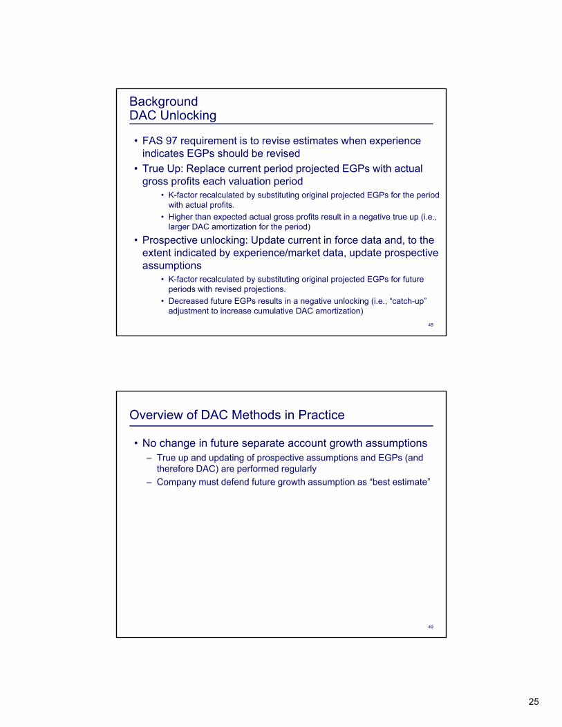
BackgroundDAC Unlocking

• FAS 97 requirement is to revise estimates when experience indicates EGPs should be revised

• True Up: Replace current period projected EGPs with actualTrue Up: Replace current period projected EGPs with actual gross profits each valuation period

• K-factor recalculated by substituting original projected EGPs for the period with actual profits.

• Higher than expected actual gross profits result in a negative true up (i.e., larger DAC amortization for the period)

• Prospective unlocking: Update current in force data and, to the extent indicated by experience/market data update prospective

48

extent indicated by experience/market data, update prospective assumptions

• K-factor recalculated by substituting original projected EGPs for future periods with revised projections.

• Decreased future EGPs results in a negative unlocking (i.e., “catch-up” adjustment to increase cumulative DAC amortization)

Overview of DAC Methods in Practice

• No change in future separate account growth assumptions– True up and updating of prospective assumptions and EGPs (and

therefore DAC) are performed regularly) p g y– Company must defend future growth assumption as “best estimate”

49

26

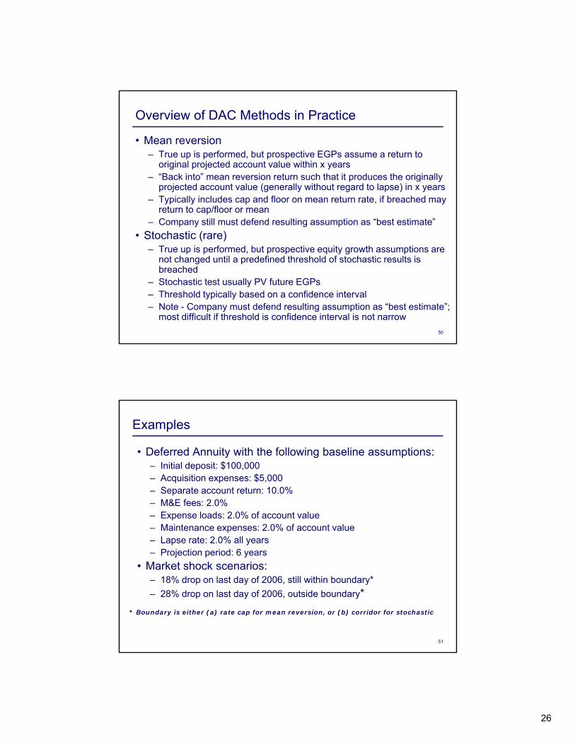
Overview of DAC Methods in Practice

• Mean reversion– True up is performed, but prospective EGPs assume a return to

original projected account value within x years“Back into” mean re ersion ret rn s ch that it prod ces the originall– “Back into” mean reversion return such that it produces the originally projected account value (generally without regard to lapse) in x years

– Typically includes cap and floor on mean return rate, if breached may return to cap/floor or mean

– Company still must defend resulting assumption as “best estimate”• Stochastic (rare)

– True up is performed, but prospective equity growth assumptions are not changed until a predefined threshold of stochastic results is

50

not changed until a predefined threshold of stochastic results is breached

– Stochastic test usually PV future EGPs– Threshold typically based on a confidence interval– Note - Company must defend resulting assumption as “best estimate”;

most difficult if threshold is confidence interval is not narrow

Examples

• Deferred Annuity with the following baseline assumptions:– Initial deposit: $100,000– Acquisition expenses: $5,000– Separate account return: 10.0%– M&E fees: 2.0%– Expense loads: 2.0% of account value– Maintenance expenses: 2.0% of account value– Lapse rate: 2.0% all years– Projection period: 6 years

• Market shock scenarios:

51

Market shock scenarios:– 18% drop on last day of 2006, still within boundary*– 28% drop on last day of 2006, outside boundary*

* Boundary is either (a) rate cap for mean reversion, or (b) corridor for stochastic

27

Examples

– No Change in Separate Account Growth Assumption – Mean Reversion– Stochastic

52

ExampleNo Change in SA Growth Assumption

Original ProjectionPV 12/31/2004 12/31/2005 12/31/2006 12/31/2007 12/31/2008 12/31/2009

Account Value EOP 100,000 103,680 107,495 111,451 115,553 119,805 EGPs 8,548 2,000 2,074 2,150 2,229 2,311 Amortization Ratio (k) 0.58496DAC B l EOP 5 000 4 230 3 356 2 366 1 252

Actual Through 2006, Annual Unlocking

PV 12/31/2004 12/31/2005 12/31/2006 12/31/2007 12/31/2008 12/31/2009Account Value EOP 100,000 103,680 79,626 82,556 85,595 88,744 EGPs 7,273 2,000 2,074 1,593 1,651 1,712 Amortization Ratio (k) 0.68752Revised DAC Balance EOP 5,000 4,025 2,921 2,060 1,090 - Revised DAC Amortization 1,375 1,426 1,095 1,135 1,177

DAC Balance EOP 5,000 4,230 3,356 2,366 1,252 - DAC Amortization 1,170 1,213 1,258 1,304 1,352

53

Reported DAC Balance 5,000 4,230 2,921 2,060 1,090 -

Actual market return of -18% in 2006 results in significant reduction in EGPs and accelerated DAC amortization (“catch up”) in 2006

28

ExampleMean Reversion


Account Value EOP 100,000 103,680 107,495 111,451 115,553 119,805 EGPs 8,548 2,000 2,074 2,150 2,229 2,311 Amortization Ratio (k) 0.58496

Actual Through 2006, 3 Year Mean Reversion

PV 12/31/2004 12/31/2005 12/31/2006 12/31/2007 12/31/2008 12/31/2009Account Value EOP 100,000 103,680 79,626 91,242 104,553 119,805 EGPs 7,658 2,000 2,074 1,593 1,825 2,091 Amortization Ratio (k) 0.65289Revised DAC Balance EOP 5,000 4,094 3,068 2,274 1,264 -


54

Revised DAC Amortization 1,306 1,354 1,040 1,191 1,365 Reported DAC Balance 5,000 4,230 3,068 2,274 1,264 -

AV drops 18% at the end of 2006, so solved for prospective separate account return assumption (21.36%) that results in projected account balance equal to original estimate in three years. (For simplicity / illustrative purposes, example shows mean reversion after lapse taken into account.)

ExampleMean Reversion


Account Value EOP 100,000 103,680 107,495 111,451 115,553 119,805 EGPs 8,548 2,000 2,074 2,150 2,229 2,311 Amortization Ratio (k) 0.58496DAC Balance EOP 5,000 4,230 3,356 2,366 1,252 - DAC Amortization 1,170 1,213 1,258 1,304 1,352

Actual Through 2006, 3 Year Mean Reversion (pierce cap)

PV 12/31/2004 12/31/2005 12/31/2006 12/31/2007 12/31/2008 12/31/2009Account Value EOP 100,000 103,680 69,673 80,263 92,463 106,518 EGPs 7,174 2,000 2,074 1,393 1,605 1,849 Amortization Ratio (k) 0.69693Revised DAC Balance EOP 5 000 4 006 2 881 2 141 1 193 -

55

Revised DAC Balance EOP 5,000 4,006 2,881 2,141 1,193 Revised DAC Amortization 1,394 1,445 971 1,119 1,289 Reported DAC Balance 5,000 4,230 2,881 2,141 1,193 -

AV drops 28% at the end of 2006, requires mean reversion rate in excess of 22% threshold, therefore 22% return assumed over next three years (alternative approach would be to return to the mean assumption of 10%)

29

ExampleStochastic Approach


Account Value EOP 100,000 103,680 107,495 111,451 115,553 119,805 EGPs 8,548 2,000 2,074 2,150 2,229 2,311 Amortization Ratio (k) 0.58496DAC B l EOP 5 000 4 230 3 356 2 366 1 252

Actual Through 2006, Stochastic (within corridor)

PV 12/31/2004 12/31/2005 12/31/2006 12/31/2007 12/31/2008 12/31/2009Account Value EOP 100,000 103,680 79,626 111,451 115,553 119,805 EGPs 8,548 2,000 2,074 2,150 2,229 2,311 Amortization Ratio (k) 0.58496Revised DAC Balance EOP 5,000 4,230 3,356 2,366 1,252 -


56

Revised DAC Balance EOP 5,000 4,230 3,356 2,366 1,252 Revised DAC Amortization 1,170 1,213 1,258 1,304 1,352 Reported DAC Balance 5,000 4,230 3,356 2,366 1,252 -

For first stochastic example, AV drops 18% at the end of 2006 – corridor is not breached so return to initial projection immediately

ExampleStochastic Approach


Account Value EOP 100,000 103,680 107,495 111,451 115,553 119,805 EGPs 8,548 2,000 2,074 2,150 2,229 2,311 Amortization Ratio (k) 0.58496DAC Balance EOP 5,000 4,230 3,356 2,366 1,252 - DAC Amortization 1,170 1,213 1,258 1,304 1,352

Actual Through 2006, Stochastic (outside corridor)

PV 12/31/2004 12/31/2005 12/31/2006 12/31/2007 12/31/2008 12/31/2009Account Value EOP 100,000 103,680 69,673 72,237 74,895 77,651 EGPs 6,817 2,000 2,074 1,393 1,445 1,498 Amortization Ratio (k) 0.73344Revised DAC Balance EOP 5 000 3 933 2 727 1 923 1 017

57

Revised DAC Balance EOP 5,000 3,933 2,727 1,923 1,017 - Revised DAC Amortization 1,467 1,521 1,022 1,060 1,099 Reported DAC Balance 5,000 4,230 2,727 1,923 1,017 -

AV drops 28% at the end of 2006 so corridor is breached and projections are unlocked back to the original assumption of 10%

30

Comparison of MethodsMethod Observations

No change in separate account growth

►Relatively easy calculation►Relatively easy to justify as “best estimate”►Most short-term volatility when actual separate accountassumption ►Most short-term volatility when actual separate account

performance differs from expected performanceMean reversion ► Relatively easy calculation

► Reduces short term volatility versus “no change” method►Occasional large unlocking, when formula produces“best estimate” company is not comfortable with

Stochastic ►Significantly decreases short term volatility, unless corridor is breached

58

breached►Valuation methodology consistent with those used for

GM*Bs►Complex calculation►Occasional very large unlocking when corridor is breached

FAS 133 for EIAs

31

EIAs under FAS 133

• Bifurcate equity component from host contract

• Equity component valuation– Black scholes– Full stochastic valuation– Option budget method

H t l t t l AV l ED t i

60

• Host equals total AV less ED at issue• Future valuation of host based on accrual at

“solved for” rate to reach maturity value

ED Valuation Methods

• Black Scholes– Works well for current option component valuation– Simple calculation– Cannot be used directly to value future option

components in more complex contracts• Full stochastic analysis

– All insurance cash flows projected over a range of risk neutral stochastic scenarios

61

neutral stochastic scenarios– At each future option component purchase date, Black

Scholes valuation can be used to value new option components within stochastic projection

– Complex

32

ED Valuation Methods

• Option Budget Method– Simpler than stochastic, but allows for valuation of future

option componentsoption components– Commonly used industry method– Assumes constant “budget” for purchase of future option

components– Constant budget (% of AV) used to determine future

account additions

62

– Expected payments to policyholders in excess of guarantee valued using risk free rates

EIA Valuation Example

• Initial deposit of $100,000• Guaranteed return of 3% on 90% of initial deposit• 10 year contract with annual reset• No surrender charges• Risk free rate at 3%, plus 1% credit spread*• Option budget calculated at 4.5% based on

stochastic analysis

63

stochastic analysis

* Credit adjustment added based on requirements of FAS 157, which will be discussed in detail in a later presentation

33


AV paid GV paid Benefits PVYear AV GMSV Guar AV Lapse Persist on lapse on lapse (Excess) Excess

100,000 90,000 11 104,635 92,700 100,000 1% 0.990 1,046 1,000 46 45 2 109,485 95,481 100,000 2% 0.970 2,168 1,980 188 174 3 114,559 98,345 100,000 3% 0.941 3,334 2,911 424 377 4 119,869 101,296 101,296 4% 0.903 4,512 3,813 699 598 5 125,425 104,335 104,335 5% 0.858 5,666 4,713 953 783 6 131,239 107,465 107,465 6% 0.807 6,758 5,534 1,224 968 7 137,322 110,689 110,689 7% 0.750 7,755 6,251 1,504 1,143 8 143,686 114,009 114,009 8% 0.690 8,625 6,843 1,781 1,302 9 150,346 117,430 117,430 9% 0.628 9,340 7,295 2,045 1,437

10 157,315 120,952 120,952 100% 0.000 98,818 75,977 22,841 15,431

148 024 116 318 31 706 22 255

64

148,024 116,318 31,706 22,255


• Resulting initial ED: $22,255• Resulting host contract: $77,745• Host contract therefore accreted at 4.52%

(guaranteed maturity value of $120,952/$77,356)^ (1/10)

• At future durations, host contract based on accretion at 4.52% and option value based on

65

revaluation at current market conditions

34

• This presentation contains general information only and is based on the experiences and research of Deloitte practitioners. Deloitte is not, by means of this presentation, rendering business, financial, investment, or other professional advice or services. This presentation is not a substitute for such professional advice or services, nor should it be used as a basis for any decision or action that may affect your business. Before making any decision or taking any action that may affect your business, you should consult a qualified professional advisor. Deloitte, its affiliates, and relatedentities shall not be responsible for any loss sustained by any person who relies on this presentationentities shall not be responsible for any loss sustained by any person who relies on this presentation.

• As used in this presentation, “Deloitte” means Deloitte Consulting LLP, a subsidiary of Deloitte LLP. Please see www.deloitte.com/us/about for a detailed description of the legal structure of Deloitte LLP and its subsidiaries.

• Copyright © 2010 Deloitte Development LLC, All rights reserved.

66

u.s. gaap & ifrs: today and tomorrow sept. 13-14, 2010 · pdf fileu.s. gaap & ifrs:...

Documents