U.S. Stock Market Crash Risk, 1926 - 2006

David S. Bates

University of Iowa and theNational Bureau of Economic Research

October 9, 2008

Preliminary and incomplete; please do not cite.

Abstract

This paper applies the Bates (RFS, 2006) methodology to the problem of estimatingand filtering time-changed Lévy processes, using daily data on stock market excessreturns over 1926-2006. In contrast to density-based filtration approaches, themethodology recursively updates the associated conditional characteristic functionsof the latent variables. The paper examines how well time-changed Lévyspecifications capture stochastic volatility, the “leverage” effect, and the substantialoutliers occasionally observed in stock market returns. The paper also finds that theautocorrelation of stock market excess returns varies substantially over time,necessitating an additional latent variable when analyzing historical data on stockmarket returns.

Henry B. Tippie College of BusinessUniversity of IowaIowa City, IA 52242-1000

Tel.: (319) 353-2288Fax: (319) 335-3690email: david-bates@uiowa.eduWeb: www.biz.uiowa.edu/faculty/dbates

What is the risk of stock market crashes? Answering this question is complicated by two features

of stock market returns: the fact that conditional volatility evolves over time, and the fat-tailed

nature of daily stock market returns. Each issue affects the other. What we identify as outliers

depends upon that day’s assessment of conditional volatility. Conversely, our estimates of current

volatility from past returns can be disproportionately affected by outliers such as the 1987 crash.

In standard GARCH specifications, for instance, a 10% daily change in the stock market has 100

times the impact on conditional variance revisions of a more typical 1% move.

This paper explores whether recently proposed continuous-time specifications of time-

changed Lévy processes are a useful way to capture the twin properties of stochastic volatility and

fat tails. The use of Lévy processes to capture outliers dates back at least to Mandelbrot’s (1963)

use of the stable Paretian distribution, and there have been many others proposed; e.g., Merton’s

(1976) jump-diffusion, Madan and Seneta’s (1990) variance gamma; Eberlein, Keller and Prause’s

(1998) hyperbolic Lévy; and Carr, Madan, Geman and Yor’s (2002) CGMY process. As all of these

distributions assume identical and independently distributed returns, however, they are unable to

capture stochastic volatility.

More recently, Carr, Geman, Madan and Yor (2003) and Carr and Wu (2004) have proposed

combining Lévy processes with a subordinated time process. The idea of randomizing time dates

back to at least to Clark (1973). Its appeal in conjunction with Lévy processes reflects the increasing

focus in finance – especially in option pricing – on representing probability distributions by their

associated characteristic functions. Lévy processes have log characteristic functions that are linear

in time. If the time randomization depends on underlying variables that have an analytic conditional

characteristic function, the resulting conditional characteristic function of time-changed Lévy

processes is also analytic. Conditional probability densities, distributions, and option prices can then

be numerically computed by Fourier inversion of simple functional transforms of this characteristic

function.

2

1Li, Wells and Yu (2006) use MCMC methods to estimate some models in which Lévyshocks are added to various stochastic volatility models. However, the additional Lévy shocks arei.i.d., rather than time-changed.

Thus far, empirical research on the relevance of time-changed Lévy processes for stock

market returns has largely been limited to the special cases of time-changed versions of Brownian

motion and Merton’s (1976) jump-diffusion. Furthermore, there has been virtually no estimation

of newly proposed time-changed Lévy processes solely from time series data.1 Papers such as Carr

et al (2003) and Carr and Wu (2004) have relied on option pricing evidence to provide empirical

support for their approach, rather than providing direct time series evidence. The reliance on options

data is understandable. Since the state variables driving the time randomization are not directly

observable, time-changed Lévy processes are hidden Markov models – a challenging problem in

time series econometrics. Using option prices potentially identifies realizations of those latent state

variables (under the assumption of correct model specification), converting the estimation problem

into the substantially more tractable problem of estimating state space models with observable state

variables.

This paper provides direct time series estimates of some proposed time-changed Lévy

processes, using the Bates (2006) approximate maximum likelihood (AML) methodology. AML is

a filtration methodology that recursively updates conditional characteristic functions of latent

variables over time given observed data. Filtered estimates of the latent variables are directly

provided as a by-product, given the close link between moments and characteristic functions. The

primary focus of the paper’s estimates is on the time-changed CGMY process, which nests various

other processes as special cases. The approach will also be compared to the time-changed jump-

diffusions previously estimated in Bates (2006).

The central issue in the study is the one stated at the beginning: what best describes the

distribution of extreme stock market movements? Such events are perforce relatively rare. For

instance, the stock market crash of October 19, 1987 was the only daily stock market

movement in the post-World War II era to exceed 10% in magnitude. By contrast, there were seven

such movements over 1929-32. Consequently, I use an extended data series of excess value-

weighted stock market returns over 1926-2006, to increase the number of observed outliers.

3

A drawback of using an extended data set is the possibility that the data generating process

may not be stable over time. Indeed, this paper identifies one such instability, in the autocorrelation

of daily stock market returns. The instability is addressed directly, by treating the autocorrelation

as another latent state variable to be estimated from observed stock market returns. Autocorrelation

estimates appear to be nonstationary, and peaked at the extraordinarily high level of 35% in 1971,

before trending downwards to the near-zero values observed since 2002.

Overall, the time-changed CGMY process is found to be a parsimonious alternative to the

Bates (2006) approach of using finite-activity stochastic-intensity jumps drawn from a mixture of

normals, although the fits of the two approaches are not dramatically different. Interestingly, one

cannot reject the hypothesis that stock market crash risk is adequately captured by a time-changed

version of the Carr-Wu (2003) log-stable process. That model’s implications for upside risk,

however, are strongly rejected, with the model severely underpredicting the frequency of large

positive outliers.

Section I of the paper progressively builds up the time series model used in estimation.

Section I.1 discusses basic Lévy processes and describes the processes considered in this paper.

Section I.2 discusses time changes, the equivalence with stochastic volatility, and further

modifications of the data generating process to capture leverage effects and time-varying

autocorrelations. Section I.3 describes how the model is estimated, using the Bates (2006) AML

estimation methodology for hidden Markov models.

Section II describes the data on excess stock market returns over 1926-2006, and presents

the estimates of parameters and filtered estimates of latent autocorrelations and volatility. Section

III presents option pricing implications, while Section IV concludes.

4

2Carr et al (2003) call the “unit time log characteristic function.” Bertoin (1996) usesthe characteristic exponent, which takes the form .

I. Time-changed Lévy processes

I.1 Lévy processes

A Lévy process is an infinitely divisible stochastic process; i.e., one that has independent and

identically distributed increments over non-overlapping time intervals of equal length. The Lévy

processes most commonly used in finance have been Brownian motion and the jump-diffusion

process of Merton (1976), but there are many others. All Lévy processes other than Brownian

motions can be viewed as extensions of jump processes. These processes are characterized by their

Lévy density , which gives the intensity (or frequency) of jumps of size x. Alternatively and

equivalently, Lévy processes can be described by their generalized Fourier transform

where u is a complex-valued element of the set for which (1) is well-defined. If is real,

is the characteristic function of , while is the cumulant generating function of

. Its linearity in time follows from the fact that Lévy processes have i.i.d. increments.

Following Wu (2006), the function will be called the cumulant exponent of .2

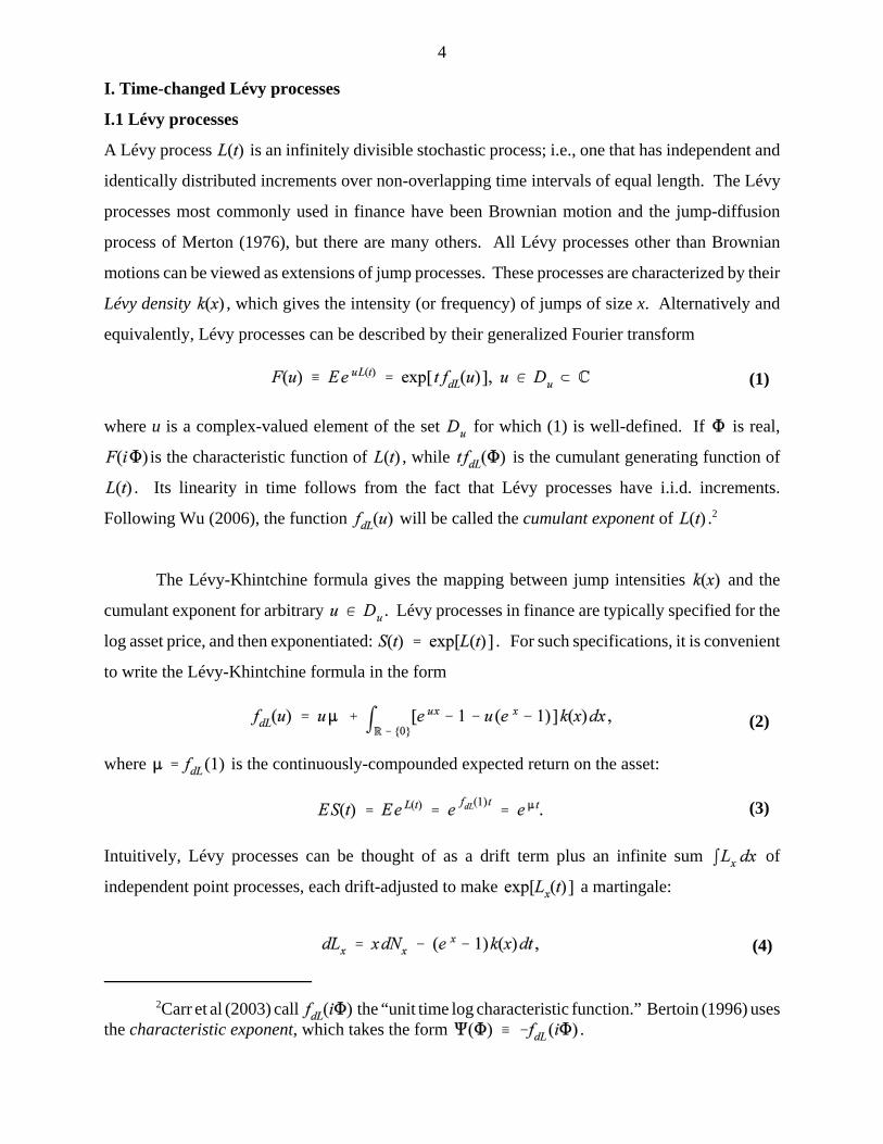
The Lévy-Khintchine formula gives the mapping between jump intensities and the

cumulant exponent for arbitrary . Lévy processes in finance are typically specified for the

log asset price, and then exponentiated: . For such specifications, it is convenient

to write the Lévy-Khintchine formula in the form

where is the continuously-compounded expected return on the asset:

Intuitively, Lévy processes can be thought of as a drift term plus an infinite sum of

independent point processes, each drift-adjusted to make a martingale:

(1)

(2)

(3)

(4)

5

where is an integer-valued Poisson counter with intensity that counts the occurrence of

jumps of fixed size x. The log characteristic function of a sum of independent point processes is the

sum of the log characteristic functions of the point processes, yielding equation (2).

As discussed in Carr et al (2002), Lévy processes are finite-activity if , and

infinite-activity otherwise. Finite-activity jumps imply there is a non-zero probability that no jumps

will be observed within a given time interval. Lévy processes are finite-variation if

, and infinite-variation otherwise. An infinite-variation process has sample paths

of infinite length – a property also of Brownian motion. All Lévy processes must have finite

, in order to be well-behaved, but need not have finite variance –

the stable distribution being an counterexample. A priori, all financial prices must be finite-activity

processes, since price changes reflect a finite (but large) number of market transactions. However,

finite-activity processes can be well approximated by infinite-activity processes, and vice versa; e.g.,

the Cox, Ross and Rubinstein (1979) finite-activity binomial approximation to Brownian motion.

Activity and variation will therefore be treated as empirical specification issues concerned with

identifying which functional form best fits daily stock market returns.

I will consider two particular underlying Lévy processes for log asset prices. The first is

Merton (1976)’s combination of a Brownian motion plus finite-activity normally distributed jumps:

where is a Wiener process,

is a Poisson counter with intensity ,

is the normally distributed jump conditional upon a jump occurring, and

is the expected percentage jump size conditional upon a jump.

The associated intensity of jumps of size x is

while the cumulant exponent takes the form

(5)

(6)

6

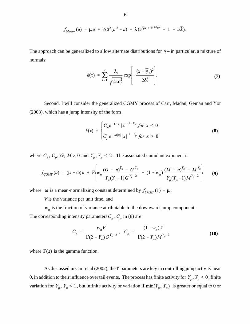
The approach can be generalized to allow alternate distributions for – in particular, a mixture of

normals:

Second, I will consider the generalized CGMY process of Carr, Madan, Geman and Yor

(2003), which has a jump intensity of the form

where and . The associated cumulant exponent is

where is a mean-normalizing constant determined by ;

V is the variance per unit time, and

is the fraction of variance attributable to the downward-jump component.

The corresponding intensity parameters in (8) are

where is the gamma function.

As discussed in Carr et al (2002), the parameters are key in controlling jump activity near

0, in addition to their influence over tail events. The process has finite activity for , finite

variation for , but infinite activity or variation if is greater or equal to 0 or

(7)

(8)

(9)

(10)

7

1, respectively. The model conveniently nests many models considered elsewhere. For instance,

includes the finite-activity double exponential jump model of Kou (2002), while

includes the variance gamma model of Madan and Seneta (1990). As and

approach 2, the CGMY process converges to a diffusion, and the cumulant exponent converges to

the corresponding quadratic form

As G and M approach 0 (for arbitrary , ), the Lévy density (8) approaches the infinite-

variance log stable process advocated by Mandelbrot (1963), with a “power law” property for

asymptotic tail probabilities. The log-stable special case proposed by Carr and Wu (2003) is the

limiting case with only negative jumps ( ). While infinite-variance for log returns, percentage

returns have finite mean and variance under the log-stable specification.

One can also combine Lévy processes, to nest alternative specifications within a broader

specification. Any linear combination of Lévy densities for is also

a valid Lévy density, and generates an associated weighted cumulant exponent of the form

.

I.2 Time-changed Lévy processes and stochastic volatility

Time-changed Lévy processes generate stochastic volatility by randomizing time in equation (1).

Since the log transform (1) can be written as

for any finite-variance Lévy process, randomizing time is fundamentally equivalent to randomizing

variance. As the connection between time changes and stochastic volatility becomes less transparent

once “leverage” effects are added, I will use a stochastic volatility (or stochastic intensity)

representation of stochastic processes.

(11)

(12)

8

The leverage effect, or correlation between asset returns and conditional variance

innovations, is captured by directly specifying shocks common to both. I will initially assume that

the log asset price follows a process of the form

The log increment consists of the continuously-compounded return, plus increments to two

exponential martingales. is a Wiener increment, while is a Lévy increment independent

of , with instantaneous variance . The term is a convexity

adjustment that converts into an exponential martingale. Further refinements will be

added below, to match properties of stock market returns more closely.

This specification has various features or implicit assumptions. First, the approach allows

considerable flexibility regarding the distribution of the instantaneous shock to asset returns,

which can be Wiener, compound Poisson, or any other fat-tailed distribution. Three underlying

Lévy processes are considered:

1) a second diffusion process independent of [Heston (1993)];

2) finite-activity jumps drawn from a normal distribution or a mixture of normals; and

3) the generalized CGMY (2003) Lévy process from (8) above.

Combinations of these processes will also be considered, to nest the alternatives.

Second, the specification assumes a single underlying variance state variable that follows

an affine diffusion, and which directly determines the variance of diffusion and jump components.

This approach generalizes the stochastic jump intensity model of Bates (2000, 2006) to arbitrary

Lévy processes.

Two alternate specifications are not considered, for different reasons. First, I do not consider

the approach of Li, Wells and Yu (2006), who model log-differenced asset prices as the sum of a

Heston (1993) stochastic volatility process and a constant-intensity fat-tailed Lévy process that

captures outliers. Bates (2006, Table 7) found the stochastic-intensity jump model fits S&P 500

returns better than the constant-intensity specification, when jumps are drawn from a finite-activity

(13)

9

normal distribution or mixture of normals. Second, the diffusion assumption for rules out

volatility-jump models, such as the exponential-jump model proposed by Duffie, Pan and Singleton

(2000) and estimated by Eraker, Johannes and Polson (2003). Such models do appear empirically

relevant, but the AML filtration methodology described below is not yet in a form appropriate for

such processes.

Define as the discrete-time return observed over horizon , and define

as the cumulant exponent of . By construction, is

a standardized cumulant exponent, with and variance . A key property of

affine models is the ability to compute the conditional generalized Fourier transform of .

This can be done by iterated expectations, conditioning initially on the future variance path:

for . This is the generalized Fourier transform of

the future spot variance and the average future variance . This is a well-known

problem (see, e.g., Bakshi and Madan (2000)), with an analytic solution if follows an affine

process. For the affine diffusion above, solves the Feynman-Kac partial differential

equation

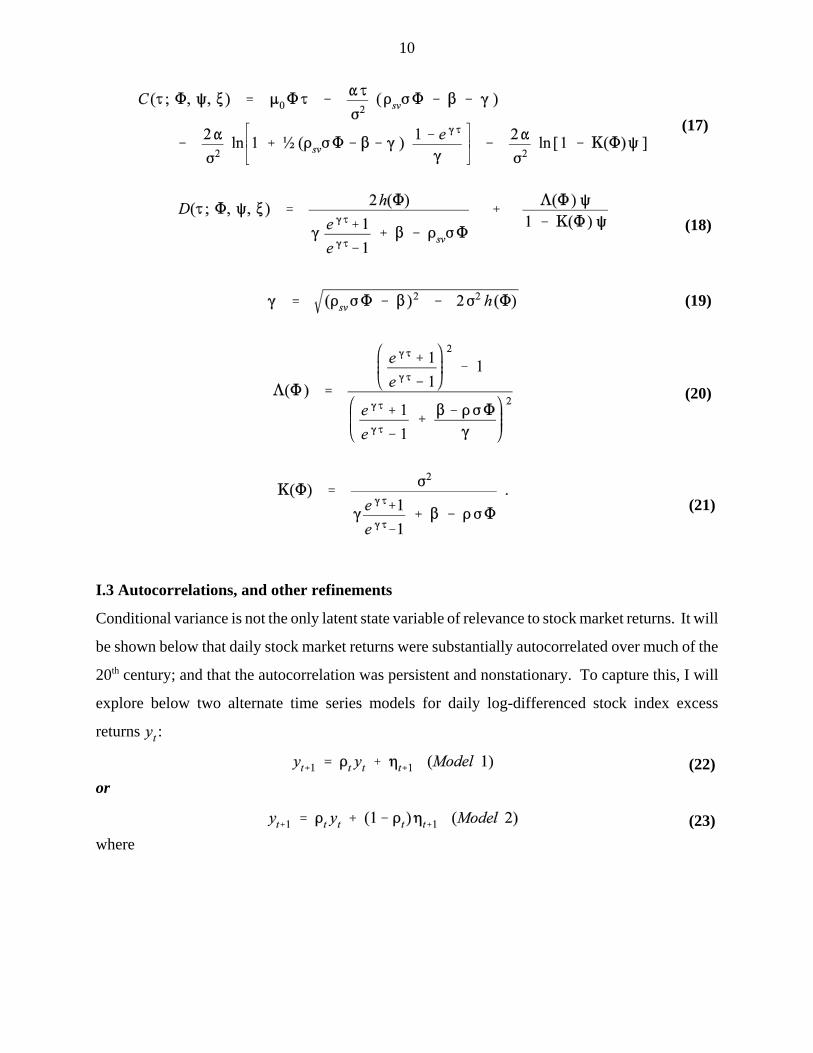
subject to the boundary condition . The solution is

where

(14)

(15)

(16)

10

(17)

(18)

(19)

(20)

(21)

I.3 Autocorrelations, and other refinements

Conditional variance is not the only latent state variable of relevance to stock market returns. It will

be shown below that daily stock market returns were substantially autocorrelated over much of the

20th century; and that the autocorrelation was persistent and nonstationary. To capture this, I will

explore below two alternate time series models for daily log-differenced stock index excess

returns :

or

where

(22)

(23)

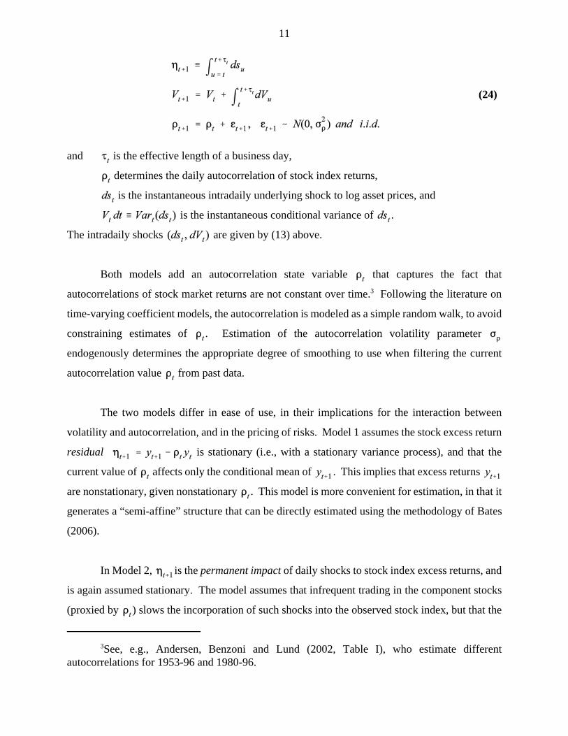
11

3See, e.g., Andersen, Benzoni and Lund (2002, Table I), who estimate differentautocorrelations for 1953-96 and 1980-96.

and is the effective length of a business day,

determines the daily autocorrelation of stock index returns,

is the instantaneous intradaily underlying shock to log asset prices, and

is the instantaneous conditional variance of .

The intradaily shocks are given by (13) above.

Both models add an autocorrelation state variable that captures the fact that

autocorrelations of stock market returns are not constant over time.3 Following the literature on

time-varying coefficient models, the autocorrelation is modeled as a simple random walk, to avoid

constraining estimates of . Estimation of the autocorrelation volatility parameter

endogenously determines the appropriate degree of smoothing to use when filtering the current

autocorrelation value from past data.

The two models differ in ease of use, in their implications for the interaction between

volatility and autocorrelation, and in the pricing of risks. Model 1 assumes the stock excess return

residual is stationary (i.e., with a stationary variance process), and that the

current value of affects only the conditional mean of . This implies that excess returns

are nonstationary, given nonstationary . This model is more convenient for estimation, in that it

generates a “semi-affine” structure that can be directly estimated using the methodology of Bates

(2006).

In Model 2, is the permanent impact of daily shocks to stock index excess returns, and

is again assumed stationary. The model assumes that infrequent trading in the component stocks

(proxied by ) slows the incorporation of such shocks into the observed stock index, but that the

(24)

12

4Jukivuolle (1995) distinguishes between the “observed” and “true” stock index when tradingis infrequent, and proposes using a standard Beveridge-Nelson decomposition to identify the latter.This paper differs in assuming that the parameters of the ARIMA process for the observed stockindex are not constant.

5Gallant, Rossi and Tauchen (1992) use a similar approach, and also estimate monthlyseasonals.

index ultimately responds fully once all stocks have traded.4 It will be shown below that this model

is more consistent with LeBaron’s (1992) observation that stock market volatility and

autocorrelations appear inversely related. Furthermore, the model is more suitable for pricing risks;

i.e., identifying the equity premium, or the (affine) risk-neutral process underlying options. The

current value of affects both the conditional mean and higher moments of , resulting in a

significantly different filtration procedure for estimating from past excess returns. The time

series model is not affine, but this paper develops a transformation of variables that makes filtration

and estimation tractable.

Both models build upon previous time series and market microstructure research into stock

market returns. For instance, the effective length of a business day is allowed to vary based upon

various periodic effects. In particular, day-of-the-week effects, weekends, and holidays are

accommodated by estimated time dummies that allow day-specific variation in . In addition, time

dummies were estimated for the Saturday morning trading available over 1926-52, and for the

Wednesday exchange holidays in the second half of 1968 that are the focus of French and Roll

(1986).5 Finally, the stock market closings during the “Bank Holiday” of March 3-15,1933 and

following the September 11, 2001 attacks were treated as - and -year returns, respectively.

Treating the 1933 Bank Holiday as a 12-day interval is particularly important, since the stock market

rose 15.5% when the market re-opened on March 15. September 17, 2001 saw a smaller movement,

of -4.7%.

For Model 1, the cumulant generating function of future returns and state variable

realizations conditional upon current values is analytic, and of the semi-affine form

13

where , and

and are given in (17) and (18) above.

For model 2, the cumulant generating function is of the non-affine form

given the shocks to are scaled by .

I.3 Filtration and maximum likelihood estimation

If the state variables were observed along with returns, it would in principle be possible to

evaluate the joint transition densities of the data and the state variable evolution by Fourier inversion

of the joint conditional characteristic function , and to use this in a maximum

likelihood procedure to estimate the parameters of the stochastic process. However, since

are latent rather than directly observed, this is a hidden Markov model that must be estimated by

other means.

For Model 1, the assumptions that the cumulant generating function (23) is affine in the

latent state variables implies that the hidden Markov model can be filtered and estimated

using the approximate maximum likelihood (AML) methodology of Bates (2006). The AML

procedure is a filtration methodology that recursively updates the conditional characteristic functions

of the latent variables and future data conditional upon the latest datum. Define

as the data observed up through period t, and define

(25)

(26)

(27)

14

as the joint conditional characteristic function that summarizes what is known at time t about

. The density of the observation conditional upon can be computed by Fourier

inversion of its conditional characteristic function:

Conversely, the joint conditional characteristic function needed for the next

observation can be updated given by the characteristic-function equivalent of Bayes’ rule:

The algorithm begins with an initial joint characteristic function and proceeds

recursively through the entire data set, generating the log likelihood function used

in maximum likelihood estimation. Filtered estimates of the latent variables can be computed from

derivatives of the joint conditional moment generating function, as can higher conditional moments:

The above procedure, if implementable, would permit exact maximum likelihood function

estimation of parameters. However, the procedure would require storing and updating the entire

function based on point-by-point univariate numerical integrations. As such a procedure

would be slow, the AML methodology instead approximates at each point in time by a

moment-matching joint characteristic function, and updates the approximation based upon updated

estimates of the moments of the latent variables. Given an approximate prior and a datum

, (27) is used to compute the posterior moments of , which are then used to create

an approximate . The overall procedure is analogous to the Kalman filtration procedure

of updating conditional means and variances of latent variables based upon observed data, under the

assumption that those variables and the data have a conditional normal distribution. However, the

equations (26) and (27) identify the optimal nonlinear moment updating rules for a given prior

, whereas Kalman filtration uses linear rules. It will be shown below that this modification in

(28)

(29)

(30)

15

filtration rules is important when estimating latent autocorrelations and variances under fat-tailed

Lévy processes. Furthermore, Bates (2006) proves that the iterative AML filtration is numerically

stable, and shows that it performs well in estimating parameters and latent variable realizations.

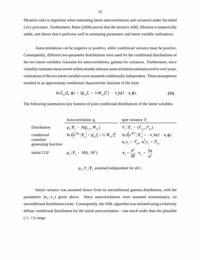
Autocorrelations can be negative or positive, while conditional variance must be positive.

Consequently, different two-parameter distributions were used for the conditional distributions of

the two latent variables: Gaussian for autocorrelations, gamma for variances. Furthermore, since

volatility estimates mean-revert within months whereas autocorrelation estimates evolve over years,

realizations of the two latent variables were assumed conditionally independent. These assumptions

resulted in an approximate conditional characteristic function of the form

The following summarizes key features of joint conditional distributions of the latent variables.

Autocorrelation spot variance

Distribution

conditionalcumulantgenerating function

initial CGF

assumed independent for all t.

Initial variance was assumed drawn from its unconditional gamma distribution, with the

parameters given above. Since autocorrelations were assumed nonstationary, no

unconditional distribution exists. Consequently, the AML algorithm was initiated using a relatively

diffuse conditional distribution for the initial autocorrelation – one much wider than the plausible

(-1, +1) range.

(31)

16

6By contrast, the FFT approach used in Carr et al (2002) requires 16,384 functionalevaluations.

The parameters – or, equivalently the moments

– summarize what is known about the latent variables. These were updated daily using the latest

observation and equations (26) - (27). For each day, 5 univariate integrations were required:

1 for the density evaluation in (26), and 4 for the mean and variance evaluations in (27). An upper

was computed for each integral which upper truncation error would be less than in magnitude.

The integrands were then integrated over to a relative accuracy of , using

IMSL’s adaptive Gauss-Legendre quadrature routine DQDAG and exploiting the fact that the

integrands for negative are the complex conjugates of the integrands evaluated at positive .

On average between 234 and 448 evaluations of the integrand were required for each integration.6

The non-affine specification in Model 2 necessitates additional

restrictions upon the distribution of latent . In particular, it is desirable that the scaling factor

be nonnegative, so that the lower tail properties of originating in the underlying Lévy

specifications do not influence the upper tail properties of . Consequently, the distribution of

latent for Model 2 is modeled as inverse Gaussian – a 2-parameter unimodal distribution with

conditional mean and variance . Appendix A derives the resultant filtration procedure

for this model, exploiting a useful change of variables procedure. The filtration is initiated at

, and it is again assumed that and are conditionally independent.

II. Properties of U.S. stock market returns, 1926 - 2006

II.1 Data

The data used in this study are daily cum-dividend excess returns on the CRSP value-weighted index

over January 2, 1926 through December 29, 2006; a total of 20,919 excess returns. The CRSP

value-weighted returns are very similar to returns on the (value-weighted) S&P Composite Index,

which began in 1928 with 90 stocks and was expanded on March 1, 1957 to its current 500-stock

structure. Indeed, the correlation between the CRSP value-weighted returns and S&P 500 returns

was .9987 over 1957-2006. The CRSP series was preferred to S&P data partly because it begins

two years earlier, but also because the S&P Composite Index is only reported to two decimal places,

17

7Estimates from other specifications were virtually identical, with estimates typically within±0.01 of the CGMY model’s estimates.

8Saturday trading was standard before 1945. Over 1945-51, it was eliminated in summermonths, and was permanently eliminated on June 1, 1952.

9As the time dummy estimates are estimated jointly with the volatility and autocorrelationfiltrations, the estimates of weekend variances with versus without Saturday trading control for anydivergences in volatility and autocorrelation levels in the two samples.

which creates significant rounding error issues for the low index values observed in the 1930’s.

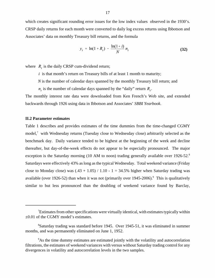
CRSP daily returns for each month were converted to daily log excess returns using Ibbotson and

Associates’ data on monthly Treasury bill returns, and the formula

where is the daily CRSP cum-dividend return;

is that month’s return on Treasury bills of at least 1 month to maturity;

N is the number of calendar days spanned by the monthly Treasury bill return; and

is the number of calendar days spanned by the “daily” return .

The monthly interest rate data were downloaded from Ken French’s Web site, and extended

backwards through 1926 using data in Ibbotson and Associates’ SBBI Yearbook.

II.2 Parameter estimates

Table 1 describes and provides estimates of the time dummies from the time-changed CGMY

model,7 with Wednesday returns (Tuesday close to Wednesday close) arbitrarily selected as the

benchmark day. Daily variance tended to be highest at the beginning of the week and decline

thereafter, but day-of-the-week effects do not appear to be especially pronounced. The major

exception is the Saturday morning (10 AM to noon) trading generally available over 1926-52.8

Saturdays were effectively 43% as long as the typical Wednesday. Total weekend variance (Friday

close to Monday close) was (.43 + 1.05) / 1.10 - 1 = 34.5% higher when Saturday trading was

available (over 1926-52) than when it was not (primarily over 1945-2006).9 This is qualitatively

similar to but less pronounced than the doubling of weekend variance found by Barclay,

(32)

18

Litzenberger and Warner (1990) in Japanese markets when Saturday half-day trading was permitted.

Barclay et al lucidly discuss market microstructure explanations for the increase in variance.

Holidays also did not have a strong impact on the effective length of a business day – with

the exception of holiday weekends spanning 4 calendar days. Consistent with French and Roll

(1986), 2-day returns spanning the Wednesday exchange holidays in 1968 (Tuesday close to

Thursday close) had a variance not statistically different from a typical 1-day Wednesday return, but

substantially less than the 1 + .94 = 1.94 two-day variance observed for returns from Tuesday close

to Thursday close in other years. Overall, the common practice of ignoring day-of-the-week effects,

weekends, and holidays when analyzing the time series properties of daily stock market returns

appears to be a reasonable approximation, provided the data exclude Saturday trading.

Table 2 reports estimates for various specifications, while Figure 1 presents associated

normal probability plots for model 1. As noted above, all models capture the leverage effect by a

correlation with the diffusion shock to conditional variance. The models diverge in their

specifications of the Lévy shocks orthogonal to the variance innovation. The first two models

(SVJ1, SVJ2) have a diffusion for small asset return shocks, plus finite-activity normally-distributed

jumps to capture outliers. The other models examine the generalized time-changed CGMY model,

along with specific parameter restrictions or relaxations.

The SVJ1 and SVJ2 results largely replicate the results in Bates (2006). The SVJ1 model

has symmetric normally-distributed jumps with standard deviation 3% and time-varying jump

intensities that occur on average = 3.2 jumps per year. As shown in Figure 1, this jump

risk assessment fails to capture the substantial 1987 crash. By contrast, the SVJ2 model adds a

second jump component that directly captures the 1987 outlier. The resulting increase in log

likelihood from 75,044.60 to 75,049.07 is statistically significant under a likelihood ratio test, with

a marginal significance level of 3.0%.

The various CGMY models primarily diverge across the specification of the

parameters – whether they are set to specific levels, and whether they diverge for the intensities of

positive versus negative jumps. The DEXP model with is conceptually similar to the

19

10This was also tested by imposing in the YY model and optimizing over otherparameters. The resulting log likelihood was 75,052.72, insignificantly different from theunconstrained 75,052.90. While setting G to zero was not permitted, given the assumption of finitevariance, a value of implies negligible exponential dampening of the intensity function(8) over the [-.20, 0] observed range of negative log stock market excess returns, and is thereforeobservationally equivalent to the log stable specification.

jump-diffusion model SVJ1, but uses instead a finite-activity double exponential distribution for

jumps. Despite the fatter-tailed specification, Figure 1 indicates the DEXP model has difficulties

comparable to SVJ1 in capturing the ‘87 crash. The VG model replaces the finite-activity double

exponential distribution with the infinite-activity variance process ( ), and does

marginally better in fit. Both models include a diffusion component, which captures 73-74% of the

variance of the orthogonal Lévy shock .

Models Y, YY, YY_J, and LS involve pure-jump specifications for the orthogonal Lévy

process , without a diffusion component. Overall, higher values of Y fit the data better –

especially the 1987 crash, which ceases to be an outlier under these specifications. Relaxing the

restriction leads to some improvement in fit, with the increase in log likelihood (YY versus

Y) having a P-value of 1.8%. Point estimates of the jump parameters governing

downward jump intensities diverge sharply from the parameters governing upward

jump intensities when the restriction is relaxed, although standard errors are large. The

dampening coefficient is not significantly different from zero, implying one cannot reject the

hypothesis that the downward-jump intensity is from a stochastic-intensity version of the Carr-Wu

(2003) log-stable process.10 By contrast, the upward intensity is estimated as a finite-activity jump

process – which, however, still overestimates the frequency of big positive outliers (Figure 1, sixth

panel).

Motivated by option pricing issues, Carr and Wu (2003) advocate using a log-stable

distribution with purely downward jumps. An approximation to this model generated by setting

and fits stock market returns very badly. The basic problem is that while the LS

model does allow positive asset returns, it severely underestimates the frequency of large positive

returns. This leads to a bad fit for the upper tail (Figure 1, last panel). Furthermore, it will be shown

below that volatility and autocorrelation estimates are adversely effected following large positive

20

returns by the model’s assumption that such returns are unlikely. However, the YY estimates

indicate that the Carr-Wu specification can be a useful component of a model, provided the upward

jump intensity function is modeled separately.

Some nested models were also estimated, to examine the sensitivity of the YY model to

specific features of the data. For instance, unrestricted CGMY models generate at least one Y

parameter in the infinite-activity, infinite-variation range [1, 2], and typically near the diffusion

value of 2. This suggests that the models may be trying to capture considerable near-zero activity.

However, adding an additional diffusion component to the time-changed YY Lévy specification to

capture that activity separately (model YY_D) led to no improvement in fit. Similarly, the

possibility that YY estimates might be affected substantially by the extreme 1987 crash was tested

by adding an independent finite-activity normally-distributed jump component capable (as in the

SVJ2 model) of capturing that outlier. The resulting fit (model YY_J) was not a statistically

significant improvement over the YY model.

Apart from the LS model, all models have similar estimates for the parameters determining

the conditional mean and stochastic variance evolution. The parameter is not significantly

different from zero, indicating no evidence over 1926-2006 that the equity premium depended upon

the level of conditional variance. Latent variance mean-reverts towards an estimated average level

, with a half-life about 2 months, and a volatility of variance estimate at about .36.

The half-life estimates are similar to those in Bates (2006, Table 8) for excess stock market returns

over 1953-1996. However, the level and volatility of variance are higher than the 1953-96 estimates

of and .25, respectively. The divergence is almost assuredly attributable to differences in

data sets – in particular, to the inclusion of the turbulent 1930's in this study.

Overall, Figure 1 suggests the differences across the alternate fat-tailed specifications are

relatively minor. The models SVJ1, DEXP, VG, and LS appear somewhat less desirable, given their

failure to capture the largest outliers. However, the SVJ2, Y, and YY specifications appear to fit

about the same. Furthermore, all models appear to have some specification error (deviations from

linearity) in the range and in the upper tail ( ). The sources of specification

error are not immediately apparent. One possibility is that the jump intensity functions are too

21

tightly parameterized, given the large amount of data. Another explanation is the data generating

process may have changed over time, and that data from the 1930's and 1940's have little relevance

for stock market risk today. Some support for this latter explanation is provided by Bates (2006,

Figure 3), who finds less evidence of specification error for models estimated over 1953-96. These

alternate possibilities will be explored further in future versions of this paper.

II.3 Autocorrelation estimates

That stock indexes do not follow a random walk was recognized explicitly by Lo and MacKinlay

(1988), and implicitly by various earlier practices in variance and covariance estimation designed

to cope with autocorrelated returns; e.g., Dimson (1979)’s lead/lag approach to beta estimation. The

positive autocorrelations typically estimated for stock index returns are commonly attributed to stale

prices in the stocks underlying the index. A standard practice in time series analysis is to pre-filter

the data by fitting an ARMA specification; see, e.g., Jukivuolle (1995). Andersen, Benzoni and

Lund (2002), for instance, use a simple MA(1) specification to remove autocorrelations in S&P 500

returns over 1953-96; a data set subsequently used by Bates (2006).

The approach of prefiltering the data was considered unappealing in this study, for several

reasons. First, the 1926-2006 interval used here is long, with considerable variation over time in

market trading activity and transactions costs, and structural shifts in the data generating process are

probable. Indeed, Andersen et al (2002, Table 1) find autocorrelation estimates from their full 1953-

96 sample diverge from estimates for a 1980-96 subsample. Second, ARMA packages use a mean

squared error criterion that is not robust to the fat tails observed in stock market returns.

Consequently, autocorrelations were treated as an additional latent variable, to be estimated jointly

with the time series model (22).

Given that the prior distribution is assumed , it can be shown that the

autocorrelation filtration algorithm (27) for Model 1 updates conditional moments as follows:

(33)

(34)

22

11Similar equations were derived by Masreliez (1975), while the overall moment-matchingfiltration methodology has been termed “robust Kalman filtration.” See Schick and Mitter (1994)for a literature review.

12See LeBaron (1992, Figure 1) for annual estimates of the daily autocorrelation of S&Pcomposite index returns over 1928-1990.

If were conditionally normal, the log density would be quadratic in , and (30) would

be the linear updating of Kalman filtration. More generally, the conditionally fat-tailed properties

of are explicitly recognized in the filtration.11 The partials of log densities can be computed

numerically by Fourier inversion.

Figures 2 illustrates the autocorrelation filtrations estimated under various models. For

model 1, the autocorrelation revision is fairly similar to a Kalman-filtration approach for

observations within a ±2% range – which captures most observations, given a unconditional daily

standard deviation around 1%. However, the optimal filtration for fat-tailed distributions is to

downweight the information from returns larger than 2% in magnitude. The exception is the Carr-

Wu log-stable specification (LS). Since that model assumes returns have a fat lower tail but not a

particularly fat upper tail, its optimal filtration downweights the information in large negative returns

but not in large positive returns.

The autocorrelation filtration under Model 2 is substantially different. Since

in that model, large observations of are attributable either to large

values of (small values of ), or to large values of the Lévy shocks captured by . The

resulting filtration illustrated in the lower panels of Figure 2 is consequently sensitive to medium-

size movements in a fashion substantially different from the Model-1 specifications.

Figure 3 presents filtered estimates of the daily autocorrelation from the YY model, and the

divergences from those estimates for other models. The most striking result is the extraordinarily

pronounced increase in autocorrelation estimates from 1941 - 1971, with a peak of 35% reached in

June 1971. Estimates from other models give comparable results, as do crude sample autocorrelation

estimates using a 1- or 2-year moving window.12 After 1971, autocorrelation estimates fell steadily,

23

13I am indebted to Ruslan Goyenko for pointing this out.

14As estimates have substantial positive skewness, the median is substantially below themean estimate of reported in Table 2.

and became insignificantly different from zero after 2002. This broad pattern is observed both for

Models 1 and 2, although the precise estimates diverge given the different filtration methodologies.

The reasons for the evolution in autocorrelations are unclear. Changes in trading volume

would seem the most plausible explanation, given the standard stale-price explanation. However,

Gallant, Rossi and Tauchen (1992, Figure 2) find that volume trended downward over 1928-43, but

generally increased throughout 1943-87. LeBaron (1992) finds that autocorrelations and stock

market volatility are inversely related; as is also apparent from comparing Figure 3 with Figure 5

below. Goyenko, Subrahmanyam, and Ukhov (2008, Figures 1-2) find shifts in their measures of

bond market illiquidity over 1962-2006 that parallel the stock market autocorrelation estimates,13

suggesting the evolution involves a broader issue of overall liquidity in financial markets.

Figure 3 also illustrates that the estimates of the daily autocorrelation are virtually

nonstationary, indicating that fitting ARMA processes with time-invariant parameters to stock

market excess returns is fundamentally pointless. The conditional standard deviation asymptotes

at about 4½%, implying a 95% confidence interval of ±9% for the autocorrelation estimates.

II.4 Volatility filtration

Figure 4 illustrates how the estimated conditional volatility is updated for the various

models. The conditional volatility revisions use median parameter values

for the prior gamma distribution of , implying a conditional mean that is close to

the median value observed for estimates from the YY model.14 For comparability with

GARCH analyses such as Hentschel (1995), Figure 4 shows the “news impact curve,” or revision

in conditional volatility estimates upon observing a given excess return, using the methodology of

Bates (2006, pp.931-2).

24

15An exception is Maheu and McCurdy (2004), who put a jump indicator sensitive to outliersinto a GARCH model. They find that the sensitivity of variance updating to the latest squared returnshould be reduced for outliers, for both stock and stock index returns.

16“Annualized” volatility refers to the choice of units. Since time is measured in years, is variance per year, and the daily volatility estimate of a return over a typical business day of length

years is approximately . Since variance mean-reverts with an estimated half-lifeof roughly 2 months, it is not appropriate to interpret Figure 5 as showing the volatility estimate fora 1-year investment horizon.

All news impact curves are tilted, with negative returns having a larger impact on volatility

assessments than positive returns. This reflects the leverage effect, or estimated negative correlation

between asset returns and volatility shocks. All models process the information in small-magnitude

asset returns similarly. Furthermore, almost all models truncate the information from returns larger

than 3 standard deviations. This was also found in Bates (2006, Figure 1) for the SVJ1 model,

indicating such truncation appears to be generally optimal for arbitrary fat-tailed Lévy processes.

The LS exception supports this rule. The LS model has a fat lower tail but not a fat upper tail, and

truncates the volatility impact of large negative returns but not of large positive returns. The fact

that volatility revisions are not monotonic in the magnitude of asset returns is perhaps the greatest

divergence of these models from GARCH models, which almost invariably specify a monotonic

relationship.15 However, since moves in excess of ±3 standard deviations are rare, both approaches

will generate similar volatility estimates most of the time.

Figure 5 presents the filtered estimates of conditional annualized volatility over 1926-2006

from the YY model 2, as well as the associated conditional standard deviation.16 Volatility

estimates from other models (except SV & LS) are similar – as, indeed, is to be expected from the

similar volatility updating rules in Figure 4. The conditional standard deviation is about 2.8%,

indicating a 95% confidence interval of roughly ±4.6% in the annualized volatility estimates.

Because of the 81-year time scale, the graph actually shows the longer-term volatility dynamics not

captured by the model, as opposed to the intra-year volatility mean reversion with 2-month half-life

that is captured by the model. Most striking is, of course, the turbulent market conditions of the

1930's, unmatched by any comparable volatility in the post-1945 era. The graph indicates the 1-

25

17The inadequacies of AR(1) representations of conditional variance are already reasonablywell-known in volatility research, and have also motivated research into long-memory processes.

factor stochastic variance model is too simple, and suggests that multifactor specifications of

variance evolution are worth exploring.17

II.5 Unconditional distributions

A further diagnostic of model specification is the models’ ability or inability to match the

unconditional distribution of returns – in particular, the tail properties of unconditional distributions.

Mandelbrot (1963, 2004), for instance, argues that empirical tails satisfy a “power law”: tail

probabilities plotted against absolute returns approach a straight line when plotted on a log-log

graph. This empirical regularity underlies Mandelbrot’s advocacy of the stable Paretian distribution,

which possesses this property and is nested within the CGMY model for .

Mandelbrot’s argument is premised upon i.i.d. returns, but the argument can in principle be extended

to time-changed Lévy processes. Conditional Lévy densities time-average; if the conditional

intensity of moves of size x is , the unconditional frequency of moves of size x is .

Since unconditional probability density functions asymptotically approach the unconditional Lévy

densities for large , while unconditional tail probabilities approach the corresponding integrals

of the unconditional Lévy densities, examining unconditional distributions may still be useful.

Figures 6a provides model-specific estimates of unconditional probability density functions of stock

market excess return residuals, as well as data-based estimates from a histogram. Given the day-of-

the-week effects reported in Table 1, the unconditional density functions are a horizon-dependent

mixture of densities, with mixing weights set equal to the empirical frequencies. The substantial

impact of the 1987 crash outlier upon parameter estimates is apparent. The SVJ2 estimates treat that

observation as a unique outlier, while the CGMY class of models progressively fatten the lower tail

as greater flexibility is permitted for the lower tail parameter . As noted above, the lower tail

approaches the Carr-Wu (2003) log-stable (LS) estimate. However, the LS model is unable to

capture the frequency of large positive outliers. All models closely match the empirical

26

18Conditional variance sample paths were simulated using the approach of Bates (2006,Appendix A.6), while Lévy shocks conditional upon intradaily average variance and data-baseddaily time horizons were generated via an inverse CDF methodology. The two observationscorresponding to the market closings in 1933 and 2001 were omitted.

unconditional density function in the ±3% range where most observations occur; and all models

underestimate the frequency of moves of 3% - 7% in magnitude.

Figure 6b provides similar estimates for unconditional lower and upper tail probabilities. In

addition, 1000 sample paths of stock market excess return residuals over 1926-2006 were simulated

via a Monte Carlo procedure using YY parameter estimates, in order to provide confidence intervals

on tail probability estimates.18 Unsurprisingly, the confidence intervals on extreme tail events are

quite wide. The underestimation of moves of 3% - 7% in magnitude is again apparent, and is

statistically significant. This rejection of the YY model does not appear attributable to

misspecification of the Lévy density , which in Figure 1 captures conditional densities

reasonably well. Rather, the poor unconditional fit in Figures 6a and 6b appears due to

misspecification of volatility dynamics. Half of the 3-7% moves occurred over 1929 - 1935 – a

sustained period with volatility exceeding 30% (see Figure 5) that simulated volatility realizations

from the 1-factor variance process of equation (13) cannot match.

Figure 7 plots model-specific tail probability estimates for the YY model on the log-log scales

advocated by Mandelbrot, along with data-specific quantiles for 20,004 stock market residuals that

have roughly a 1-day estimated time horizon (±25%). The lower tail probability does indeed

converge to the unconditional tail intensity

where and is the incomplete gamma function.

Furthermore, given G estimates near 0, is roughly a power function, implying near linearity

when plotted on a log-log scale.

(35)

27

However, the graph indicates that the convergence of tail probabilities to the tail intensity

occurs only for observations in excess of 5% in magnitude – roughly 5 standard deviations. As this

is outside the range of almost all data, it does not appear that log-log scales provide a useful

diagnostic of model specification and tail properties. This is partly due to stochastic volatility,

which significantly slows the asymptotic convergence of unconditional tail probabilities to

for large . Absent stochastic volatility ( ), the tail probabilities of an i.i.d. YY Lévy

process converge to for observations roughly in excess of 3% in magnitude (3 standard

deviations).

No power law properties are observed for upper tail probabilities, given substantial estimated

exponential dampening. The failure of both lower and upper unconditional tail probabilities to

capture the frequency of moves of 3-7% in magnitude is again apparent, and statistically significant.

III. Option pricing implications

Do these alternative models imply different option prices? Exploring this issue requires identifying

the appropriate pricing of equity, jump, and stochastic volatility risks. Furthermore, the presence

of substantial and stochastic autocorrelation raises issues not previously considered when pricing

options. In particular, the observed stock index level underlying option prices can be stale, while

the relevant volatility measure over the option’s lifetime is also affected. The variance of the sum

of future stock market returns is not the sum of the variances when returns are autocorrelated.

To examine these issues, I will focus upon Model 2, with its distinction between the observed

CRSP value-weighted stock index and an underlying true index level that would be observed were

all component stock prices continuously updated. Furthermore, I will use the myopic power utility

pricing kernel specification of Bates (2006) for pricing the various risks:

where is the permanent shock to the log stock market level given above in equations (24) - (25).

This specification constrains both the equity premium estimated under the objective time series

(36)

28

19Carr and Wu (2003) specify a log-stable process for the risk-neutral process underlyingoption prices. This can be generated by a time-changed CGMY process for the actual process withonly downward jumps, and with .

20Wu (****) discusses this transformation.

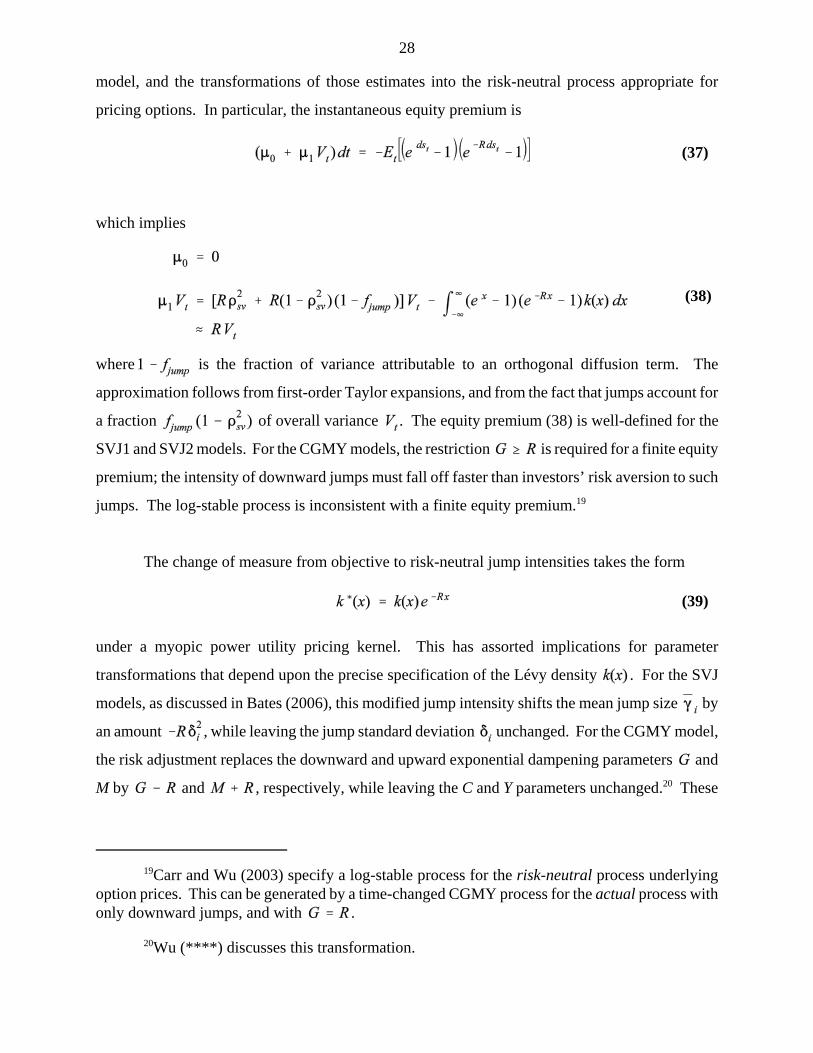
model, and the transformations of those estimates into the risk-neutral process appropriate for

pricing options. In particular, the instantaneous equity premium is

which implies

where is the fraction of variance attributable to an orthogonal diffusion term. The

approximation follows from first-order Taylor expansions, and from the fact that jumps account for

a fraction of overall variance . The equity premium (38) is well-defined for the

SVJ1 and SVJ2 models. For the CGMY models, the restriction is required for a finite equity

premium; the intensity of downward jumps must fall off faster than investors’ risk aversion to such

jumps. The log-stable process is inconsistent with a finite equity premium.19

The change of measure from objective to risk-neutral jump intensities takes the form

under a myopic power utility pricing kernel. This has assorted implications for parameter

transformations that depend upon the precise specification of the Lévy density . For the SVJ

models, as discussed in Bates (2006), this modified jump intensity shifts the mean jump size by

an amount , while leaving the jump standard deviation unchanged. For the CGMY model,

the risk adjustment replaces the downward and upward exponential dampening parameters and

M by and , respectively, while leaving the C and Y parameters unchanged.20 These

(37)

(38)

(39)

29

risk adjustments alter the and functions in equation (14). Table (*) summarizes the

various parameter transformations.

The potential impact of autocorrelations upon option prices will be addressed by examining

prices of options on S&P 500 futures. I assume that stock index futures prices respond

instantaneously and fully to the arrival of news, whereas lack of trading in the underlying stocks

delays the incorporation of that information into the reported CRSP and S&P 500 stock index levels.

Furthermore, I assume that index arbitrageurs effectively eliminate any stale prices in the component

stocks on days when futures contracts expire, so that stale prices do not affect the cash settlement

feature of stock index futures. MacKinlay and Ramaswamy (1988) provide evidence supportive of

both assumptions.

These assumptions have the following implications under Model 2:

1. the observed futures price underlying options on S&P 500 futures is not stale;

2. given the AR(1) specification for stock index excess returns in equation (22), log futures

price innovations are approximately the intradaily innovations of equation (13):

Consequently, European options on stock index futures can be priced directly using a risk-neutral

version of (40) – which is affine, simplifying option evaluation considerably. Furthermore, option

prices do not depend upon , except indirectly through the impact of autocorrelation filtration upon

the filtration of latent variance . Following Bates (2006), European call prices on an S&P 500

futures contract can be priced as

(40)

(41)

30

21The parameters are replaced by , while the function is replaced by a risk-adjusted function that captures the risk-adjusted jump intensities fromequation (33).

22Wu (2006) proposes an alternate pricing kernel with negative risk aversion for downsiderisk, thereby automatically imposing .

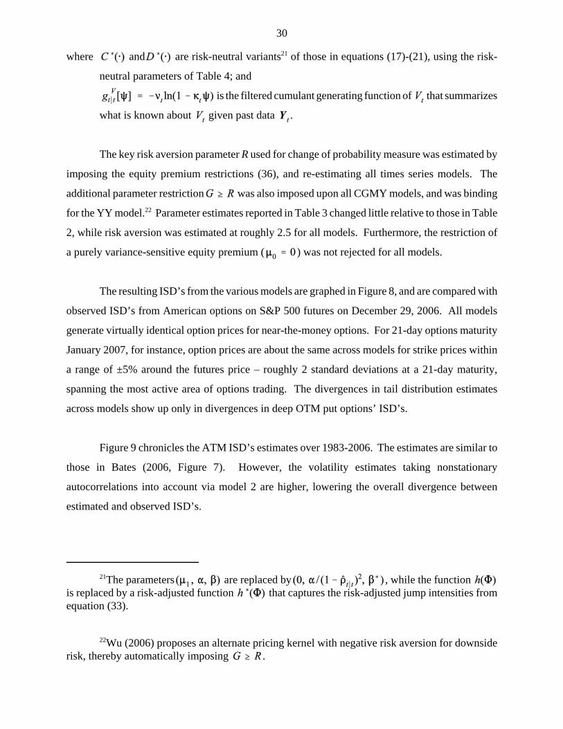
where and are risk-neutral variants21 of those in equations (17)-(21), using the risk-

neutral parameters of Table 4; and

is the filtered cumulant generating function of that summarizes

what is known about given past data .

The key risk aversion parameter R used for change of probability measure was estimated by

imposing the equity premium restrictions (36), and re-estimating all times series models. The

additional parameter restriction was also imposed upon all CGMY models, and was binding

for the YY model.22 Parameter estimates reported in Table 3 changed little relative to those in Table

2, while risk aversion was estimated at roughly 2.5 for all models. Furthermore, the restriction of

a purely variance-sensitive equity premium ( ) was not rejected for all models.

The resulting ISD’s from the various models are graphed in Figure 8, and are compared with

observed ISD’s from American options on S&P 500 futures on December 29, 2006. All models

generate virtually identical option prices for near-the-money options. For 21-day options maturity

January 2007, for instance, option prices are about the same across models for strike prices within

a range of ±5% around the futures price – roughly 2 standard deviations at a 21-day maturity,

spanning the most active area of options trading. The divergences in tail distribution estimates

across models show up only in divergences in deep OTM put options’ ISD’s.

Figure 9 chronicles the ATM ISD’s estimates over 1983-2006. The estimates are similar to

those in Bates (2006, Figure 7). However, the volatility estimates taking nonstationary

autocorrelations into account via model 2 are higher, lowering the overall divergence between

estimated and observed ISD’s.

31

IV. Summary and Conclusions

This paper provides estimates of the time-changed CGMY (2003) Lévy process, and compares them

to the time-changed finite-activity jump-diffusions previously considered by Bates 2006). Overall,

both models fit stock market excess returns over 1926-2006 similarly. However, the CGMY

approach is slightly more parsimonious, and is able to capture the 1987 crash without resorting to

the “unique outlier” approach of the SVJ2 model. The CGMY model achieves this with a (slightly)

dampened power law specification for negative jump intensities that is observationally equivalent

to a time-changed Carr-Wu (2003) infinite-variance log-stable specification. However, the time-

changed log-stable model is found to be incapable of capturing the substantial positive jumps also

observed in stock market returns, which the more general time-changed CGMY model handles

better. All models still exhibit some conditional and unconditional specification error, the sources

of which have not yet been fully established.

The paper also documents some structural shifts over time in the data generating process.

Most striking is the apparently nonstationary evolution of the first-order autocorrelation of daily

stock market returns, which rose from near-zero in the 1930's to 35% in 1971, before drifting down

again to near-zero values after 2002. Longer-term trends in volatility are also apparent in the filtered

estimates, suggesting a need for multifactor models of conditional variance. Whether there appear

to be structural shifts in the parameters governing the distribution of extreme stock market returns

will be examined in future versions of this paper.

Finally, it is important when estimating latent state variables to use filtration methodologies

that are robust to the fat-tailed properties of stock market returns. Standard GARCH models lack

this robustness, and generate excessively large estimates of conditional variance after large stock

market movements.

32

References

Andersen, Torben G., Luca Benzoni, and Jesper Lund (2002). "An Empirical Investigation ofContinuous-Time Equity Return Models." Journal of Finance 57, 1239-1284.

Bakshi, Gurdip and Dilip B. Madan (2000). "Spanning and Derivative-Security Valuation." Journalof Financial Economics 55, 205-238.

Barclay, Michael J., Robert H. Litzenberger, and Jerold B. Warner (1990). "Private Information,Trading Volume, and Stock-Return Variances." Review of Financial Studies 3, 233-254.

Bates, David S. (2006). "Maximum Likelihood Estimation of Latent Affine Processes." Review ofFinancial Studies 19, 909-965.

Bertoin, Jean (1996). Lévy Processes, Cambridge: Cambridge University Press.

Carr, Peter, Hélyette Geman, Dilip B. Madan, and Marc Yor (2002). "The Fine Structure of AssetReturns: An Empirical Investigation." Journal of Business 75, 305-332.

Carr, Peter, Hélyette Geman, Dilip B. Madan, and Marc Yor (2003). "Stochastic Volatility for LévyProcesses." Mathematical Finance 13, 345-382.

Carr, Peter and Liuren Wu (2003). "The Finite Moment Log Stable Process and Option Pricing."Journal of Finance 58, 753-777.

Carr, Peter and Liuren Wu (2004). "Time-changed Lévy Processes and Option Pricing." Journalof Financial Economics 71, 113-141.

Clark, Peter K. (1973). "A Subordinated Stochastic Process Model with Finite Variance forSpeculative Prices." Econometrica 41, 135-155.

Cox, John C., Stephen A. Ross, and Mark Rubinstein (1979). "Option Pricing: A SimplifiedApproach." Journal of Financial Economics 7, 229-263.

Dimson, Elroy (1979). "Risk Measurement When Shares are Subject to Infrequent Trading."Journal of Financial Economics 7, 197-226.

Duffie, Darrell, Jun Pan, and Kenneth J. Singleton (2000). "Transform Analysis and Asset Pricingfor Affine Jump-Diffusions." Econometrica 68, 1343-1376.

Eberlein, Ernst, Ulrich Keller, and Karsten Prause (1998). "New Insights into Smile, Mispricing,and Value at Risk: The Hyperbolic Model." Journal of Business 71, 371-405.

Eraker, Bjorn, Michael Johannes, and Nicholas G. Polson (2003). "The Impact of Jumps inVolatility and Returns." Journal of Finance 58, 1269-1300.

33

French, Kenneth R. and Richard Roll (1986). "Stock Return Variances: The Arrival of Informationand the Reaction of Traders." Journal of Financial Economics 17, 5-26.

Gallant, A. Ronald, Peter E. Rossi, and George Tauchen (1992). "Stock Prices and Volume."Review of Financial Studies 5, 199-242.

Hentschel, Ludger (1995). "All in the Family: Nesting Symmetric and Asymmetric GARCHModels." Journal of Financial Economics 39, 71-104.

Heston, Steve L. (1993). "A Closed-Form Solution for Options with Stochastic Volatility withApplications to Bond and Currency Options." Review of Financial Studies 6, 327-344.

Jukivuolle, Esa (1995). "Measuring True Stock Index Value in the Presence of Infrequent Trading."Journal of Financial and Quantitative Analysis 30, 455-464.

Kou, Steve (2002). "A Jump Diffusion Model for Option Pricing." Management Science 48,1086-1101.

LeBaron, Blake D. (1992). “Some Relations between Volatility and Serial Correlations in StockReturns.” Journal of Business 65, 199-219.

Li, Haitao, Martin T. Wells, and Cindy L. Yu (2006). "A Bayesian Analysis of Return Dynamicswith Stochastic Volatility and Lévy Jumps." University of Michigan working paper, January.

Lo, Andrew W. and A. Craig MacKinlay (1988). "Stock Market Prices Do Not Follow RandomWalks: Evidence from a New Specification Test." Review of Financial Studies 1, 41-66.

Maheu, John M. And Thomas H. McCurdy (2004). “News Arrival, Jump Dynamics and VolatilityComponents for Individual Stock Returns.” Journal of Finance 59, 755-793.

Madan, Dilip B. and Eugene Seneta (1990). "The Variance Gamma (V.G.) Model for Share MarketReturns." Journal of Business 63, 511-525.

Mandelbrot, Benoit B. (1963). "The Variation of Certain Speculative Prices." Journal of Business36, 394-419.

Mandelbrot, Benoit B. and Richard L. Hudson (2004). The (mis)Behavior of Markets: A FractalView of Risk, Ruin, and Reward. New York: Basic Books.

Masreliez, C. J. (1975). “Approximate Non-Gaussian Filtering with Linear State and ObservationRelations.” IEEE Transactions on Automatic Control 20, 107-110.

Merton, Robert C. (1976). "Option Pricing When Underlying Stock Returns are Discontinuous."Journal of Financial Economics 3, 125-144.

SBBI Yearbook, 2006. Chicago: R. G. Ibbotson Associates.

34

Schick, Irvin C. And Sanjoy K. Mitter (1994). “Robust Recursive Estimation in the Presence ofHeavy-tailed Observation Noise.” The Annals of Statistics 22, 1045-1080.

Wu, Liuren (2006). "Dampened Power Law: Reconciling the Tail Behavior of Financial SecurityReturns." Journal of Business 79, 1445-1473.

35

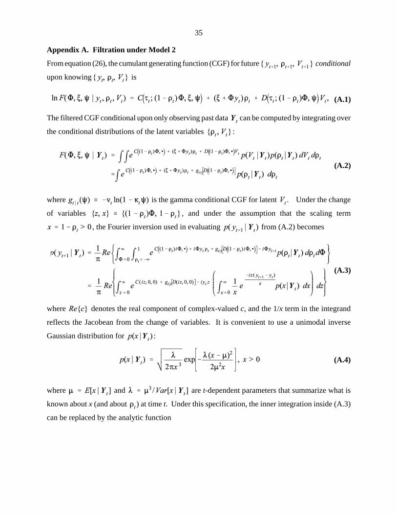
Appendix A. Filtration under Model 2

From equation (26), the cumulant generating function (CGF) for future conditional

upon knowing is

The filtered CGF conditional upon only observing past data can be computed by integrating over

the conditional distributions of the latent variables :

where is the gamma conditional CGF for latent . Under the change

of variables , and under the assumption that the scaling term

, the Fourier inversion used in evaluating from (A.2) becomes

where denotes the real component of complex-valued c, and the 1/x term in the integrand

reflects the Jacobean from the change of variables. It is convenient to use a unimodal inverse

Gaussian distribution for :

where and are t-dependent parameters that summarize what is

known about x (and about ) at time t. Under this specification, the inner integration inside (A.3)

can be replaced by the analytic function

(A.1)

(A.2)

(A.3)

(A.4)

36

1A more “natural” choice would be to represent x by a beta distribution over the range [0, 2].That would constrain , and results in an term that involves the confluenthypergeometric U-function. However, I could not find a method for evaluating that function thatwas fast, accurate, and robust to all parameter values.

for . Consequently, evaluating (A.3) involves only univariate

numerical integration.1

Similar univariate integrations are used for filtering and conditional upon observing .

The noncentral posterior moments of are given by

where the derivatives with respect to inside the integrand can be easily evaluated from the

specifications for and in equations (17) - (18) . The posterior moments of can be

computed by taking partials of (A.2) with respect to , and then again using change of variables to

reduce the Fourier inversion to a univariate integration. The resulting posterior mean and variance

of are

where

(A.5)

(A.6)

(A.7)

(A.8)

37

and

Finally, the conditional distribution function that is used in QQ plots

takes the form

(A.9)

(A.10)

(A.11)

Table 1: Effective length of a business day, relative to 1-day Wednesday returns: 1926-2006.

NOBSModel 1 Model 2

#days Description estimate std. error estimate std. error

11111

Monday close 6 Tuesday closeTuesday close 6 Wednesday closeWednesday 6 Thursday Thursday 6 Friday Friday 6 Saturday (1926-52)

38314037399839241141

1.021.94.93.43

(.04)

(.03)(.03)(.02)

1.031.94.92.44

(.03)

(.03) (.03)(.02)

222

Saturday close 6 Monday close (1926-52)Weekday holidayWednesday exchange holiday in 1968

112034122

1.051.25.73

(.05)(.11)(.33)

1.071.26.81

(.05)(.10)(.35)

345

Weekend and/or holidaya

Holiday weekendHoliday weekend

2755343

6

1.101.581.31

(.04)(.14)

(1.00)

1.101.561.25

(.04)(.13)(.93)

21518

aIncludes one weekday holiday (August 14 - 17, 1945)

Table 2A: Estimates of parameters affecting the conditional means and volatilities. Data: daily CRSP value-weighted excess returns, 1926-2006. See equations (6) - (10), (13), and (25) for definitions of parameters. Models with combine Lévy jump processes with an additionalindependent diffusion, with variance proportions , respectively. Standard errors are in parentheses.

Model 1:

Modelln L

Conditional mean Stochastic volatility

HL(mths)

SVSVJ1SVJ2DEXPVGYYYYY_DYY_JLS

75,044.6075,049.0775,047.6275,049.4875,050.1275,052.9075,052.9075,054.9475,005.53

.040 (.015)

.042 (.015)

.044 (.015)

.042 (.015)

.042 (.015)

.042 (.015)

.042 (.015)

.041 (.015)

.019 (.015)

.94 (.91)

.87 (.92)

.79 (.91)

.91 (.91)

.91 (.92)

.87 (.91)

.87 (.91)

.97 (.92)1.71 (.78)

.030 (.006)

.030 (.007)

.030 (.006)

.030 (.006)

.030 (.006)

.030 (.006)

.030 (.006)

.030 (.007)

.031 (.007)

.155 (.005)

.155 (.005)

.156 (.005)

.156 (.005)

.157 (.008)

.159 (.008)

.159 (.010)

.154 (.005)

.165 (.005)

4.33 (.40)4.34 (.37)4.25 (.40)4.25 (.39)3.90 (.38)4.00 (.38)4.01 (.38)3.99 (.38)4.52 (.39)

.370 (.011)

.371 (.011)

.370 (.012)

.368 (.012)

.350 (.019)

.362 (.019)

.363 (.021)

.350 (.012)

.405 (.011)

-.642 (.020)-.642 (.020)-.588 (.020)-.587 (.020)-.577 (.032)-.572 (.031)-.572 (.036)-.586 (.020)-.554 (.020)

1.9 (.2)1.9 (.2)2.0 (.2)2.0 (.2)2.1 (.2)2.1 (.2)2.1 (.2)2.1 (.2)1.8 (.2)

Model 2:

SVSVJ1SVJ2DEXPVGYYYLS

74,999.8775,092.1075,096.6875,094.2075,094.7075,093.6875,097.2075,045.48

-.014 (.020) .033 (.020) .037 (.020) .034 (.020) .034 (.020) .036 (.021) .033 (.020) .053 (.019)

3.04 (.90)1.69 (1.04)1.25 (.89)1.44 (.90)1.42 (.90)1.35 (.90)1.44 (.90)1.50 (.76)

.043 (.005).036 (.005).036 (.005).036 (.005).037 (.005).036 (.005).036 (.005).031 (.003)

.170 (.004)

.171 (.004)

.172 (.004)

.171 (.004)

.171 (.004)

.172 (.007)

.172 (.006)

.174 (.005)

8.01 (.57)5.80 (.49)5.71 (.49)5.67 (.49)5.56 (.48)5.18 (.46)5.23 (.47)4.68 (.41)

.562 (.015)

.457 (.015)

.456 (.015)

.452 (.015)

.447 (.016)

.432 (.021)

.437 (.018)

.436 (.015)

-.658 (.017)-.674 (.018)-.673 (.018)-.625 (.018)-.623 (.018)-.613 (.027)-.613 (.022)-.576 (.019)

1.0 (.1)1.4 (.1)1.4 (.1)1.5 (.1)1.6 (.1)1.6 (.1)1.6 (.1)1.8 (.2)

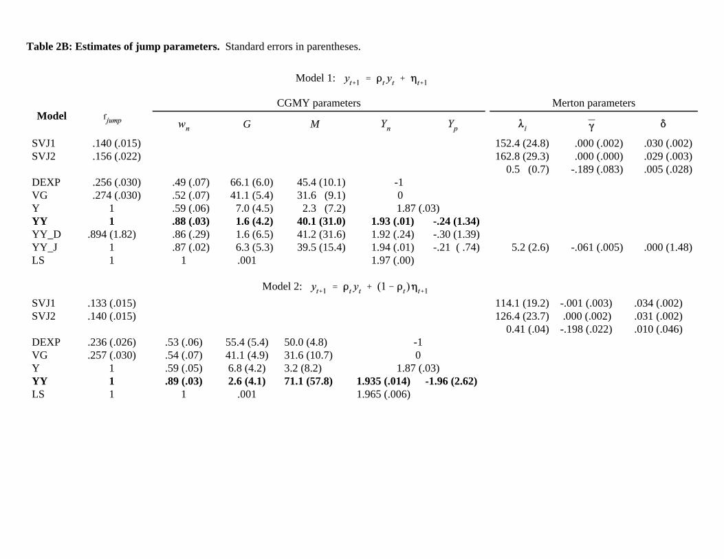
Table 2B: Estimates of jump parameters. Standard errors in parentheses.

Model 1:

ModelCGMY parameters Merton parameters

G M

SVJ1 .140 (.015) 152.4 (24.8) .000 (.002) .030 (.002)SVJ2 .156 (.022) 162.8 (29.3)

0.5 (0.7) .000 (.000)-.189 (.083)

.029 (.003)

.005 (.028)DEXP .256 (.030) .49 (.07) 66.1 (6.0) 45.4 (10.1) -1 VG .274 (.030) .52 (.07) 41.1 (5.4) 31.6 (9.1) 0 Y 1 .59 (.06) 7.0 (4.5) 2.3 (7.2) 1.87 (.03)YY 1 .88 (.03) 1.6 (4.2) 40.1 (31.0) 1.93 (.01) -.24 (1.34)YY_D .894 (1.82) .86 (.29) 1.6 (6.5) 41.2 (31.6) 1.92 (.24) -.30 (1.39)YY_J 1 .87 (.02) 6.3 (5.3) 39.5 (15.4) 1.94 (.01) -.21 ( .74) 5.2 (2.6) -.061 (.005) .000 (1.48)LS 1 1 .001 1.97 (.00)

Model 2: SVJ1 .133 (.015) 114.1 (19.2) -.001 (.003) .034 (.002)SVJ2 .140 (.015) 126.4 (23.7)

0.41 (.04) .000 (.002)-.198 (.022)

.031 (.002)

.010 (.046)DEXP .236 (.026) .53 (.06) 55.4 (5.4) 50.0 (4.8) -1VG .257 (.030) .54 (.07) 41.1 (4.9) 31.6 (10.7) 0Y 1 .59 (.05) 6.8 (4.2) 3.2 (8.2) 1.87 (.03)YY 1 .89 (.03) 2.6 (4.1) 71.1 (57.8) 1.935 (.014) -1.96 (2.62)LS 1 1 .001 1.965 (.006)

Table 3: Parameter estimates with constrained equity premium , . Model 2:

Modelln L

Test of

(p-value)

Conditional mean Stochastic volatility

HL(mths)

SVSVJ1SVJ2DEXPVGYYY

74,999.6775,091.0875,095.6675,093.1275,093.5675,092.4575,096.11

.527

.153

.153

.142

.131

.117

.140

2.57 (.63)2.52 (.62)2.47 (.65)2.53 (.62)2.61 (.59)2.49 (.62)2.44 (.63)

2.57 (.63)2.52 (.62)2.48 (.65)2.51 (.62)2.61 (.59)2.49 (.62)2.44 (.63)

.043 (.005).037 (.005).037 (.005).037 (.005).037 (.005).037 (.005).037 (.005)

.171 (.004)

.172 (.004)

.172 (.004)

.172 (.004)

.172 (.004)

.173 (.007)

.173 (.005)

7.78 (.50)6.27 (.45)6.22 (.49)6.13 (.45)6.06 (.44)5.66 (.43)5.67 (.47)

.556 (.014)

.438 (.014)

.456 (.015)

.463 (.015)

.458 (.015)

.444 (.021)

.449 (.015)

-.653 (.015)-.684 (.016)-.673 (.018)-.636 (.016)-.634 (.017)-.625 (.027)-.624 (.017)

1.1 (.1)1.3 (.1)1.4 (.1)1.4 (.1)1.4 (.1)1.6 (.1)1.5 (.1)

ModelCGMY parameters Merton parameters

G M

SVJ1 .130 (.015) 110.3 (18.8) -.001 (.003) .034 (.002)SVJ2 .137 (.026) 122.6 (20.4)

0.44 (.80) .000 (.002)-.197 (.046)

.031 (.002)

.006 (.114)DEXP .172 (.004) .54 (.07) 55.5 (5.4) 50.7 (12.3) -1VG .172 (.004) .54 (.03) 41.1 (5.0) 31.6 (9.7) 0Y 1 .61 (.05) 6.8 (4.2) 3.0 (8.5) 1.87 (.03)YY 1 .89 (.03) 2.4a 71.0 (60.7) 1.934 (.009) -1.97 (2.77)

aParameter constraint was binding.

Table 4: Change of measure under a myopic power utility pricing kernel .

Objective Risk-neutralEquity premium 0

General jump intensityMerton parameters

mean jump sizejump SD unchanged

CGMY parametersG G - R (must be $0)M M + R

unchanged

Variance processmean reversion UC mean

-5 -4 -3 -2 -1 0 1 2 3 4

0.0010.0030.01 0.02 0.05 0.10

0.25

0.50

0.75

0.90 0.95 0.98 0.99 0.9970.999

Data

Prob

abilit

yNormal Probability Plot SVJ1

-4 -3 -2 -1 0 1 2 3 4

0.0010.0030.01 0.02 0.05 0.10

0.25

0.50

0.75

0.90 0.95 0.98 0.99 0.9970.999

Data

Pro

babi

lity

Normal Probability Plot SVJ2

-5 -4 -3 -2 -1 0 1 2 3

0.0010.0030.01 0.02 0.05 0.10

0.25

0.50

0.75

0.90 0.95 0.98 0.99 0.9970.999

Data

Pro

babi

lity

Normal Probability Plot DEXP

-4 -3 -2 -1 0 1 2 3

0.0010.0030.01 0.02 0.05 0.10

0.25

0.50

0.75

0.90 0.95 0.98 0.99 0.9970.999

Data

Pro

babi

lity

Normal Probability Plot VG

Figure 1. Normal probability plots for thenormalized returns ,for different models. Diagonal line: theoretical quantiles conditional upon

correct specification +: Empirical quantiles

-4 -3 -2 -1 0 1 2 3

0.0010.0030.01 0.02 0.05 0.10

0.25

0.50

0.75

0.90 0.95 0.98 0.99 0.9970.999

Data

Pro

babi

lity

Normal Probability Plot Y

-3 -2 -1 0 1 2 3

0.0010.0030.01 0.02 0.05 0.10

0.25

0.50

0.75

0.90 0.95 0.98 0.99 0.9970.999

Data

Pro

babi

lity

Normal Probability Plot YY

-4 -3 -2 -1 0 1 2 3 4

0.0010.0030.01 0.02 0.05 0.10

0.25

0.50

0.75

0.90 0.95 0.98 0.99 0.9970.999

Data

Pro

babi

lity

Normal Probability Plot LS

-0.8%

-0.4%

0.0%

0.4%

0.8%

-5% -3% -1% 1% 3% 5%

-0.8%

-0.4%

0.0%

0.4%

0.8%

-5% -3% -1% 1% 3% 5%

SVJ1SVJ2DEXPVGYYYLSKalman

-1.5%

-1.0%

-0.5%

0.0%

0.5%

-8% -4% 0% 4% 8% -1.5%

-1.0%

-0.5%

0.0%

0.5%

-8% -4% 0% 4% 8%

SV

SVJ1

SVJ2

DEXP

VG

Y

YY

LS

Figure 2: Autocorrelation revision conditional on observing , andconditional on

Model 1With With

Model 2

With With

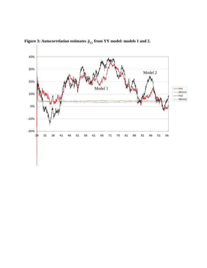
-20%

-10%

0%

10%

20%

30%

40%

26 31 36 41 46 51 56 61 66 71 76 81 86 91 96 01 06

rho1

SE(rho1)

rho2

SE(rho2)

Figure 3: Autocorrelation estimates from YY model: models 1 and 2.

Model 2

Model 1

-2%

0%

2%

4%

6%

-8 -4 0 4 8

0%

10%

20%

30%

40%

50%

26 31 36 41 46 51 56 61 66 71 76 81 86 91 96 01 06

-2%

0%

2%

4%

6%

-8 -4 0 4 8

SVSVJ1SVJ2DEXPVGYYYLS

Figure 4: News impact curves for various models

Model 1 Model 2

LS SV LS SV

Asset return, in SD units Asset return, in SD units

The graph show the revision in estimated annualized standard deviation

conditional upon observing a standardized return of magnitude .

Figure 5: Estimates of permanent volatility shocks (model 2) – YY model.

0.00001

0.0001

0.001

0.01

0.1

1

-20% -15% -10% -5% 0% 5% 10% 15%

SVJ1SVJ2DEXPVGYYYLSdata2.5%97.5%

1.E-05

1.E-04

1.E-03

1.E-02

1.E-01

1.E+00

1.E+01

1.E+02

-20% -15% -10% -5% 0% 5% 10% 15%

SVJ1SVJ2DEXPVGYYYLSdata

Figure 6a. Unconditional probability density function estimates from various models, and directdata-based estimates from a histogram (.25% cell width).

871019

SVJ2

YY

SVJ1 LS

Figure 6b. Unconditional tail probability estimates. The dotted lines give 95% confidenceintervals, based upon 1000 simulations of the 1926-2006 data set under YY parameter estimates.

0.00001

0.0001

0.001

0.01

0.1

1

0.1%1.0%10.0%100.0%0.00001

0.0001

0.001

0.01

0.1

1

0.1% 1.0% 10.0% 100.0%

Figure7. Unconditional tail probabilities and tail intensity functions versus ; log scales on both axes. Data-based estimates fromexcess returns’ residuals for 20,004 business days with estimated time horizons of approximately 1 day (±25%). Dotted lines give 95%confidence intervals, based upon 1000 simulated sample paths under YY parameter estimates.

y < 0 y > 0

data

Figure 8: Estimated and observed ISD’s for options on S&P 500 futures: Dec. 29, 2006. 95% confidence intervals for SVJ2model for parameter uncertainty (dark grey), and parameter & state uncertainty (light grey).