COMPUTER METHODS IN APPLIED MECHANICS AND ENGINEERING 55 (IYH6) 63-H7NORTH-HOLLAND

AN ADAPTIVE CHARACTERISTIC PETROV-GALERKINFINITE ELEMENT METHOD FOR CONVECTION-DOMINATED LINEAR

AND NONLINEAR PARABOLIC PROBLEMS IN TWO SPACE VARIABLES*

L. DEMKOWICZ and J.T. ODENThe Texas Institute for Computational Mechanics. The University of Texas at Austin, Austin, TX 78712.

u.s.A.

Received 31 July 1985

This paper is a continuation of previous work of the authors [2]. An adaptive scheme for the analysisof time-dependent parabolic problems defined on two-dimensional or three-dimensional space domainsis developed which is based on a Petrov-Galerkin method for spatial approximation and the method ofcharacteristics for the temporal approximation. Numerical examples are discussed which illustrate theefficiency and effectiveness of the method.

1. Introduction

In this paper we present a continuation of our previous work [2] on a class of specialPetrov-Galerkin methods for convection-dominated parabolic problems. A principal featureof the work discussed here is the generalization of the theory and algorithms developed earlierto multi-dimensional cases, with particular attention to two-dimensional cases for the sake ofclarity. We note that these extended methods also provide for the calculation of optimal testfunctions, the establishment of what we call 'extra-superconvergence' results for a modelelliptic problem, and corresponding truly local a posteriori error estimates. Finally, we showthat the merger of the proposed optimal Petrov-Galerkin scheme with the method ofcharacteristics leads to a powerful and accurate scheme for quite general parabolic and certainhyperbolic problems.

Following this introduction, we generalize the one-dimensional theory discussed in [21 to themulti-dimensional case and, using the concept of 'numerically optimal test functions', wedevelop a special Petrov-Galerkin method for treating a typical 'elliptic step' in the numericalanalysis of evolution problems. The use of special trial and test functions resulting in thecoincidence of 'semi-exact' and approximate solutions along the interelement boundaries laysthe foundation for truly local a posteriori error estimates and for the use of effective ellipticsolvers. These are discussed in Section 3. Section 4 is devoted to a brief discussion of thecharacteristic Petrov-Galerkin method, formulated in our previous work. In Se~tion 5, wegeneralize the method to systems of two nonlinear Burgers' equations. In Section 6, weaddress some important numerical considerations and, in Section 7, we present numerical

-The support of this work by ONR under Contract NOOO-14-84-K-0409 is gratefully acknowledged.

0045-7825/86/$3.50 © 1986, Elsevier Science Publishers B.V. (North-Holland)

64 L. Demkowicz, J.T Oden, A Petrov-Galerkin method for parabolic problems

results obtained by applying th{ method to representative problems. Finally, in Section 8 welist several concluding remarks.

2. Petrov-Galerkin finite element method for a model elliptic problem

We begin our study with the following simple elliptic problem given on a domain D C R 2:

lilld tI : 11-... n SlIt:1l 111 .. 1

-sL1u + u = I in D,

u= V

auan = g

on Til, (2.1)

where L1 is the Laplacian; ru and rr form two disjoint portions of the boundary aD; and fand V and g are prescribed data in n and on an respectively. The positive constantcoefficient s is implicitly assumed to be 'small'. The corresponding variational formulation is:

find u E HI(D) such that

s J VuVv dx + J uv dx = J Iv dx + J gv ds \Iv E HHf2) ,n n n fr

u = V on fll,

(2.2)

where H}·(D) = {v E HI(D) I v = 0 on rll} and dx = dx, dX2'To conSlruct a Petrov-Galerkin approximation of this problem, we introduce a finite-

dimensional approximation space X" spanned by trial functions 1/1;, and a corresponding spaceof test functions V". Assuming, for simplicity, that the function V, specifying Dirichletboundary conditions, can be spanned by traces of trial functions from X", we replace (2.2) bythe following Petrov-Galerkin approximation:

find u" E X" such that

In (2.3), it is understood that the approximate solution u" is of the form

N

U" = VII + 2: ULt/Ji'i-I

(2.3)

(2.4)

where VII E XII and uL are unknown coefficients to be determined. We also have, of course,dim VII = N.

L. Demkowicz. 1.T Oden, A Petrov-Galerkin method for parabolic problems

Subtracting (2.3) from (2.2), we obtain the well-known orthogonality condition,

65

(2.5)

(2.6)

with U - Uh E Vh which is the subspace of Xh consisting of functions satisfying homogeneouskinematic boundary conditions on T" and spanned by .pi' i = 1, ... , N.

The Petrov-Galerkin approximation (2.3) provides great flexibility in the choice of numeri-cal schemes since the space \lh of test functions is, at this point, arbitrary and, therefore, wecan tailor test functions so as to produce special properties in the approximation. Here wefollow a plan similar to that of Barrett and Morton [1] and design, for given shapefunctions .pi> i = 1,2, ... , N, 'optimal' test functions Vh as solutions of the auxiliary problem:

find ME H}(fl) such that

e J V<p Vu'; dx + J <pu'; dx = J Vel>V.pj dx V eI> E H Hfl) .n n n

We observe that Petrov-Galerkin approximations Uh obtained using these test functionspossess some important properties. In particular, by replacing 4> in (2.6) by the error U - Uh,

we get

t V(u - Uh) V.pj dx = 0, i= 1, ... ,N, (2.7)

which is recognized as the standard orthogonality condition for errors in Bubnov-Galerkinapproximations of the Poisson problem -Ju = f; the model boundary value coefficient e doesnot appear in this condition. Clearly, the use of optimal test functions leads to a method with aglobal rate of convergence in HI-seminorm which is independent of e!

On the other hand, the so-called optimal test functions v~ of (2.6), unfortunately, do nothave local support and, therefore, are essentially useless for practical calculations. An attemptat replacing these functions by new, local functions, spanning the same space Vh, as is possiblein the one-dimensional case, fails for all classical finite element trial functions in multipledimensions. To resolve this difficulty, we introduce new, very special finite elements andcorresponding trial functions which do admit a localization of the corresponding optimal testfunctions.

Toward this end, we turn to the concept of numerically optimal test functions, introduced in[2]. For simplicity and clarity, we restrict ourselves to a polygonal domain on which a fixedcoarse finite element mesh is given. We then subdivide each of the elements into a finesubmesh consisting of much smaller elements, and, in this way, also cover the original coarsemesh with a fine mesh. We call the coarse-mesh elements superelements and the elements ofthe fine mesh micro-elements. The concept is illustrated in Fig.!.

Let Xi denote a fine-grid nodal point which lies on the interelement boundary aK of twosuperelements. For each such node, we associate a special trial function .pi E W which satisfiesthe following conditions:

.p/(x}) = Oi} at each node X},

66 L. Delllkowicz, J.T Oden, A Petrov-Galerkj'l method for parabolic problems

Fig. 1. Concept of super· and micro-elements.

L Va/JVw dx = 0 V' w E W, w(Xj) = 0 for all j. (2.8)

Here W denotes a space of functions spanned by piecewise polynomial shape functionsdefined over the fine mesh. As in [2], we accept the fine-grid approximation of the solutions of(2.2) obtained with the W-space approximation as the 'semi-exact' solution; i.e., u in (2.2) isreplaced by the solution of the following problem:

find u E W such that

u = U on ru,

e J VuVw dx + J uw dx == J fw dx + J gw ds V' w E Wr,n n n rr

(2.9)

where Wr == {w E WI w == 0 on rJ.The space of trial functions Xh is now defined as the space spanned by trial functions (2.8).

We can thus eliminate all degrees of freedom corresponding to the interior nodes ofsuperelements. We also note that trial functions 1/1/ are nothing else than 'semi-exact' solutionsto the homogeneous Laplace equation with Dirichlet boundary conditions specified alonginter-superelement boundaries.

For the sake of simplicity, we shall restrict ourselves in subsequent analyses to quadrilateralmeshes with only piecewise bilinear approximations. We emphasize that the conceptsdeveloped here are much more general and apply to arbitrary finite element grids. In thiscontext, note also that with uniform refinement of superelements, the classical trial functionsassociated with nodes of the coarse grid, although not explicitly included in definition (2.8),can be spanned by functions I/1j and, therefore, form a subspace of Xh•

The approximation of (2.9) follows the same steps as described earlier. The space Xh of trialfunctions is now taken to be a subspace of Wand the 'approximate' solution, Uh, is definedonce again by (2.3), except that now the test functions Vh are taken from a space Vh imbeddedin the same 'big' space W as the space of trial functions Xh• The orthogonality condition againtakes the form (2.5), and the definition of that which we call 'numerically optimal test function'corresponding to a trial function a/Jj reads as follows:

L. Demkowicz, J. T Oden, A Petrov-Galerkill method for parabolic problems 67

(2.11)

find 6~ E W,. such lhat

E J VwV67 dx + f wv7 dx = f VwVl/1; dx 'v' wE WI" (2.10)n n n

Note also that v~ is W-equivalent to a function which satisfies the homogeneous version of theoriginal equation (or equivalently, its adjoint) (2.1) inside each of the superelements.

Contrary to the test functions VI, defined in (2.6), the 'numerically optimal test functions'can be localized. Toward this end, we associate with each of the nodes X; the correspondinglocal test function (fJ; defined by:

cP;(Xj) = O;j 'v' j = 1, ... , N,

E L Vw VcPldx + L wcP;dx = ° V w E Wr, w(xJ = 0, j = 1, ... , N.

We claim that the local functions cP; span exactly the same space Vh as the global functions 6~.To prove this, let ,5~ denote an interpolant of v~ constructed using the functions cPj.We have

ef V(6~-,5~?dx+f (6~-,5~)2dx=0,/I /I

(2.12)

since 67 - ,57 E Wr (we have (D? - ,57)(x,) = 0) and both 67 and ,57 are orthogonal (in the senseof the above scalar product) to functions from Wr vanishing along inter-superelementboundaries. Since (2.12) is equivalent to the condition M - 07 = 0, we have proved theassertion.

Thus, by using the local numerically optimal test functions cPl defined by (2.11), we achievethe orthogonality condition (2.7), which in turn implies the optimal, E-independent errorestimate (between Uh and the 'semi-exact' solution U of course!) and, which is perhaps moreimportant, leads to the same 'extra-superconvergence' result derived in the one-dimensionalcase, n:imely,

Uh = U along the interelement boundaries aK. (2.13)

To verify this remarkable result, notice that any function from W, say w, can always bedecomposed into the sum of two parts,

w = W + wo, (2.14)

where W is spanned by base functions built upon the fine mesh associated with nodes Xj

located along the coarse-grid interelement boundaries and wo(xJ) = 0, j = 1, ... ,N. From thedefinition of l/1i it follows that

L VwVl/1j dx = L VwVl/1j dx, i= 1, ... , N (2.15)

68 L Demkowicz. J. T Oden. A Petrov-Galerkin method for parabolic problems

and, therefore, if the integral c 1'\ the left-hand side of (2.15) vanishes for all 1/11> then w mustvanish as well. This is equivalent to saying that w == 0 along the inter-supcrelement boundaries.

REM ARK 2.1. Orthogonality cL'ndition (2.7) is crucial in the establishment of both the optimalerror estimate in the HI-seminorm and the extra-superconvergence result (2.13). This con-dition exploits properties of both trial and test functions. The identity (2.13), however, istotally independent of the definition of trial functions 1/1i and follows directly from the onlydefinition of tcsl functions <Pi' In particular, if we arc interested in (2.13) only, wc may dcfincdifTerenl trial functions which could conceivably be more convenient from the computationalpoint of view.

REMARK 2.2. It is not clear how the concept of the optimal but local test functions can begeneralized for the infinite-dimensional case (W = H1(fl». Intuitively, this would require acontinuum of degrees of freedom along interelement boundaries. One might be satisfied withonly an approximate localization of optimal test functions (see [1]) which would again involvea finite number of degrees of freedom but result in the loss of the extra-superconvergenceresult (2.13).

The natural reduction of the problem to one with degrees of freedom on interelementboundaries suggests a similarity of our method with hybrid methods or with boundary finiteelement methods. These and other related concepts deserve further study.

3. An adaptive Petrov-Galerkin method

3.1. A.posteriori error estimates

The extra-superconvergence result allows us to derive truly local a posteriori error estimates,it being understood that the error is a measure of the difference between Uh and semi-exactsolution (2.9).

It is easily seen that, for every superelement K, the error eh = U - Uh satisfies the conditions

eJ VehVwdx+ I ehwdx=J (f-uh)wds for every wE WK,KKK

(3.1)

where WK = {wE Wlsupp wCK}.Obviously, (3.1) is equivalcnt to a self-adjoint problem in Wk' The particular form of (3.1)

suggests the introduction of three natural norms:(1) the computable L2-residual norm

112

IIrhIlL2(K) = (t (f - Uh? dx) ; (3.2)

L. Demkowicz, J. T. Oden, A Petrov-Galerki!J method for parabolic problems

(2) the energy norm

(3) the L2-norm of the error

69

(3.3)

(3.4)

The following inequalities follow directly from the spectral decomposition of the operatorassociated with equation (3.1) (d. [2]):

(3.5)

Here AI is the smallest eigenvalue associated with the operator define~ by (3.1) and can beevaluated numerically. For practical purposes, when the mesh is fine enough, AI can bereplaced by the smallest eigenvalue of the 'continuous problem'. For instance, for a squareelement of size hand aK nFr = 0, the smallest eigenvalue is

(3.6)

Each of the two error estimates (3.5) may serve as a basis for local refinements. The energynorm (3.5)2 may, of course, be related to the L""-norm of the error

(3.7)

It is difficult, however, to estimate precisely the constant C (in terms of element size h) and,therefore, it seems to be inefficient to combine (3.7) with (3.5)2' Instead, if we insist on usingV"-error estimates, we may recall that (3.1) is equivalent to a system of linear equations, say

Aeh = 'h or eh = A-Irh' (3.8)

and after having inverted A use the classical linear algebraic estimates to estimate eh, forinstance (d. [6, p. 22])

(3.9)where

"IIA -III"" = max 2: IAi;'I·I..j .. " j= I

3.2. Mesh-refinement techniques

We propose two mesh-refinement techniques based on the results established thus far.

70 L. Demkowicz. J.T. Oden, A Petrov-Galerkin method for parabolic problems

3.2.1. Consecutive-refinement technique(i) Choose an initial mcsh and solvc the system of equations rcsulting from thc Pctrov-

Galerkin method.(ii) Using estimates (3.5) or (3.9) with a given error tolerance TaL, determine which of the

clemcnts nced refinement (1lehllK ;?l: TaL).(iii) Subdivide each of the quadri'laterals, for which the error estimate exceeds the tolerance,

into four subelements.(iv) For each of the subdivided elements, solve the local problem (2.9) (over one element

only, using the Petrov-Galerkin method again) with the known interelement nodal valuesimposed as local boundary conditions.

(v) Using the error estimates again determine which of the new elements need furtherrefinement.

(vi) If elements exist for which lIehll ~ TaL, refine them and go to step (iv); otherwise, iflIehll <TaL for all elements K, stop the process.

A typical mesh resulting from such a refinement technique is shown in Fig. 3.

.3.2.2. Complete-refinement technique(i) Choose an initial mesh and solve the system of equations resulting from the Petrov-

Galerkin method.(ii) Using the error estimates with a given error tolerance TaL, determine which of the

elemcnts requires refinement.(iii) For each of the elements for. which the error estimate exceeds TOL, solve the local

problem (2.9) using the fine mesh and standard Bubnov-Galerkin method .(iv) Stop.The first method may be more expensive and time-consuming than the second, but it

requires a minimum of machine storage. The second one, numerically much faster and moreefficient for the case TOL = 0, when all elements are refined, can be viewed as a very specialand efficient solver for problem (2.1). We will return to the problem of efficiency in Section 6.

4. The adaptive characteristic Petrov-Galerkin finite element method for convection-dominatedlinear diffusion problems

We shall now use the techniques discussed in [2] to combine the adaptive Petrov-Galerkinmethod discussed in previous sections with the method of characteristics to treat convection-dominated linear diffusion problems. We focus on evolution problems of the following type:

find u = u(x, t) sllch that

u, + C· flu - eL1u = f, x En, t E (0, T),

u(x, t) = vex, t) , x E rIA, t E (0, T) ,

auan (x, t) = g(x, t) ,

u(x,O) = uo(x),

x E rT, t E (0, T) ,

xEn.

(4.1)

L. Demkowicz, J. T Oden, A Petrov-Galerkin method for parabolic problems 71

Here e is a small positive number (€ ~ IcD; c = c(x, t) is a given transport function; Vex, t),and g(x, t) and uo(x) are boun dary and initial data respectively; and I = I(x, t) is a given sourceterm.

To solve (4.1) numerically, we first partition the time interval [0, T] according to

0= to < t1 < ... < tK == T.

Then we replace (4.1) by the following sequence of elliptic problems:

for each k == 1, ... , K find u"(x) such that

Uk - E /1t L1uk = f(x, tIl) /1t + U"-I(X(X, t,,; t"-I» in nwith boundary conditions:

u" == U on ru,

au"-=g onTT'au

(4.2)

(4.3)

Here /1t = /1tk = tIl - tk_ J' Uk-l is the solution at the previous time step for k > 1, U"-I = Uo fork = 1, and X(x, t,,; .) is the characteristic line drawn backward in time from the point (x, tic),i.e., X is the solution of the equation

dX = c(X, t) , ( < tic ,dt (4.4)

In implementing (4.3), we view the numerical scheme as a fractional step method of the lype

Du"-112Dt =0 (4.5)

where DtDt is the (absolute) derivative in the direction of the characteristic line.As the next step, we apply to each of the steps of (4.3) our adaptive Petrov-Galerkin

method. Because our scheme is to be adaptive, the dimension of V" (and V,,) will generallychange at each time step.

The method is thus defined by the following system of discrete problems:

find u~ E V" C W such that

E /1tJ Vu~ VV" dx + J u~v" dxn n

= In {I(x, tIl) /1t + U"-I(X(X, tic; t"_I»}V/I(x) dx + In gv" ds "Iv" E V", (4.6)

u~ = U on ru·

72 L. Demkowicz, J. T. Oden, A Petrov-Galerkin method for parabolic problems

Error estimates for such schell.les hased on the method of charactcristics arc derivcd in f4,71and reproduced in l2]; they ar..; indepcndent of the spacc dimension and, therefore, will not berepeated here.

Finally, let us mention that the concept of numerically optimal test functions results in an'almost' e-stable schcme; i.c., we havc

(4.7)

for certain small constant µ (dcpendent on and controllcd by tolerance TaL). For details, onceagain we refer to [2].

5. Application to Burgers' equations in 2-D

As an initial step toward the analysis of compressible and incompressible fluid mechanicsproblems, we consider the application of our method to a system of nonlinear Burgers'equations. We restrict ourselves to the Dirichlet problem:

find u = u(x, t), u = (u\ u2) such that

u, + u . Vu - eL1u = 0, x E n, t E (0, T) ,

u(x, I) = U(x, t) ,

U(x,O) = Ull(X) ,

x E an., t E (0, T), (5.1)

With the fractional step method notation in use, we may split the typical time step into twosteps:

(1) transport

U~-II2(X) = U~-I(Xh(X, tk; lk-I));

(2) diffusion (5.2)

Uh = U on an .The essential difference between this case and the one discussed in the previous section is thatthe characteristic lines are now solution-dependent.

Several schemes for constructing approximate characteristic Jines suggest themselves. In thesubsequent analysis we will restrict ourselves to the case of regular, rectangular meshes only,approximating characteristics by straight lines within each time step.

The approximation of the characteristics and the transport step is illustrated in Fig. 2. Forpositive parameters g and T] we have

L. Demkowicz, J. T Oden, A Petrov-Galerkin met/rod for parabolic problems

approximatecharacterisfic

xFig. 2. COllslruction of characteristics.

k - 1/2 k - I l:( k Ie) + ( Ie k) + t:. (k + k k k)Ujj = Ujj +~ Ui.j+I-Ujj 71 IIj+I,j-Ujj ",71 Uj+l.j+1 Ujj-Ui,}+I-Ui+I,}'

73

(5.3)

Parameters g and 71 specifying the slope of the characteristic line may be determined in threedifferent ways:

(1) explicit scheme

6.x Ie-I-~At =Uli; ,

(2) implicit scheme

6.x _ 1e-1/2- ~At -u1ij ,

(3) fully implicit scheme6.x _ Ie-~Tt -Ulij'

6.y 1e-1/2 .- 71 At = U 2;j ,

6.y Ie-71 Tt = U2ij'

(5.4)

When substituted into (5.3), the implicit scheme (5.4)2 results in a nonlinear system of twoequations for ut-1I2 which can be solved by any of the classical techniques. The use of (5.4)3couples fully both steps of our fractional method and results in a globally nonlinear schemerequiring extra iterations.

74 L. Demkowicz, 1.T OdClI, A Petrov-Ga/erkill mcthod for parabolic problems

Let us finally note that the standard requirement, that characteristic lines should neverexceed the neighboring 'cell', results in the limitation of the time step in the form of the usualCFL-condition.

6. Some numerical aspects and details

In this section, we address some computational aspects of the method, comparing inparticular the two adaplive schemes proposed in Section 3. We emphasize that the deter-mination of the trial functions I/Ji of (2.8) and test functions cPj of (2.11) require the solutionover each superelement of the corresponding boundary value problems on the fine mesh. Themain problem is not in the time required to do such a computation (we need to do this onlyonce and then apply the solutions at every time step), but rather in the storage necessary tostore these preliminary results. This suggests that elements with the same geometry should beused as much as possible in generating the coarse mesh.

Another computational difficulty has to do with the accessibility of the finite elementsolution Uh' Imagine a typical superelement consisting of, say, 16 x 16 micro-elements (see Fig.3), for which 64 boundary nodes exist and 225 internal nodes are eliminated in the Petrov-Galerkin scheme. In this case, the calculation of Uh at any internal node requires the ful1(stored) information about trial functions corresponding to the boundary nodes and results inas many as 64 multiplications. In particular, the number of operations needed to calculate theresidual (3.2) to estimate the error is so large that it turns out to be faster to resolve the localproblem over the superelement without estimating the error. On the other side, this forces usto store the whole solution, thereby increasing the storage and resulting in a method whichsuffers from many limitations of the classical Bubnov-Galerkin scheme. Thus, it seemsnecessary to develop a special technique to estimate the error and to balance the cost ofcomputation with the cost of storage. In the context of regular, rectangular meshes, we canuse, for instance, the following simple technique:

(i) Using four vertices of the rectangular element and the corresponding four nodal values,construct a bilinear function Un. Obviously, Un satisfies equation (2.8) and, therefore, is acertain linear combination of cPi corresponding to the classical bilinear approximation over theelement.

(ii) Compare the boundary values of Uh and Uh by calculating the L2(aK) error of thedifference

(6.1)

(iii) If error (6.1) is negligible (smaller than a given threshold tolerance 8), use Uh tocalculate residual (3.2); otherwise, refine the element or resolve the whole local problem,dependent on the technique being used, without calculating residual (3.2).

This two-step procedure in estimating the error seems to be very inexpensive and can begeneralized easily for other than rectangular elements.

Final1y, we address the differences between the two proposed refinement techniques. Aswas noted in Section 3, the first technique minimizes the amount of storage necessary to store

L. Demkowicz, J. T. Dden, A Petrov-Galerk itt method for parabolic problew <

I I I T I I I I I I I I I I II I I T I I I I I I I I I I I

.980 .111 .126 .1~ 5 .16', .180 . ~O!l .228 .2~8 .267 .285 J02 .J16 .326 .5Jl ~ ~(-5) (-4) (-4) (-4) (-4; (-4) (-!o) (-4) (-4) (-4 ) (-4) -4 ) (-4) (-4) (-4)

~ ~

.712(-4) .562(-4) .4JJ(-4) .325(-4) .2J6(-4) .211(-4) .600(-4) ------

.12l( -4) .120(-~) .10)(-4) --~ ~

. ~ ~II

I ~ ~

I --IIi --iI, ~ ~

I .220(-4)

~ ~

~ ~

l- I-

Fig. 3. Model elliptic problem-final, refined mesh.

75

the solution, while requiring a very complicated tree structure for code implementation. Onthe other hand, the fact that our particular formulation requires many right-hand sideevaluations, due to the necessity to update source and convective terms at each time step (see(4.6», suggests that the second scheme might be much more efficient than the first. Withelements of repeated geometry, we may factor the local stiffness matrix resulting from theBubnov-Galerkin method (and already necessary for the determination of test functions) justonce and use it to resolve all local problems in a very fast and efficient way.

For the above reasons, all the evolution problems presented in the next section are solvedusing the second method, the first scheme being used only for an elliptic example problem.

Another aspect of the method worthy of comment has to do with the elliptic character ofthe adaptive scheme and its impact on the transport step of the algorithm. In the case of thelinear problem (4.1), the characteristics depend upon the coefficient c(x, t) and variable c mustbe determined at every node of the fine mesh. For equation (5.1), however, the characteristicsdepend upon the computed solution and, therefore, allow us to use information on the

76 L. Demkowicz, J. T Oden, A Petrov-Galerkin method for parabolic problems

regularity of the solution at f\ach time step. For instance, it is easy to see that the explicitscheme (5.4)" with (5.3), results in a formula which is invariant for linear functions. In otherwords, if a solution (locally) is linear, then the corresponding convected solution for the nexttime step is linear as well. This observation may provide a basis for the development ofinexpensive methods for the calcllialion of righI-hand sides necessary in the diffusion step. Theidea of using the information on the regularity of the solution gained during the refinementprocess requires some additional study and has not yet been implemented in our programs.

7. Numerical results

7.1. Model elliptic problem

As a first example, which illustrates concepts rather than a practical case, we solve problem(2.1) with homogeneous Dirichlet boundary conditions and the right-hand side correspondingto the exact solution

whereu(x, y) = w(x)· w(y),

w(x) = -exp(- x) - exp[(1 + s )(x - 1)/s] + (A - B)x - A

(7.1)

with A, B chosen so that w(O) = w(l) = 0 and domain f2 being the square (0, 1)2. For small lO,

the solution (7.1) possesses a thin boundary layer near x = 1 and y = 1. The problem has beensolved using the 'consecutive-refinement' technique with numerical data chosen as follows:

number of superelements N = 2· 2 = 4,

s = 0.01,

TaL = 0.001.

The error estimate (3.5)) has been used without applying the simplified technique described inSection 6. The corresponding final refined mesh, together with local-error estimates and thegraph of the solution, are presented in Figs. 3 and 4.

7.2. Heat equation with a dominating convection

Following Donea ct al. [3], we consider problem (3.1) on a unit square domain n =(0, 1)2, with right-hand side J, and initial and Dirichlet boundary conditions corresponding tothe following exact solution:

where

u(r, t) = O'~t) exp[ - 2O'~t)2 (r - ro - at?] ,

O'(t) = 0'0(1 + 2st/a~)'12 .

(7.2)

The problem has been solved using the superelement technique with a regular mesh of 25

L. Demkowicz. J. T Odell. A Petrov-Galnkill method for paraholic problems

Fig. 4. Model elliptic problem-numerical solution.

77

elements, each consisting of 256 (16 x 16) micro-elements. The numerical data are as follows:

Uo = v'2/20,

a = (0.5,0.5),

E = 0.004,

threshold tolerances S = 0.008, TaL = 0.01, (compare (6.1) and Section 3.2)

a constant time step AT = 0.2.

Figs. 5, 6, 7, 8 and 9 show the evolution of the numerical solution after 1, 25, 50, 75 and 100time steps, respectively, with the corresponding mesh refinements. As the time progresses, theGaussian hill travels along the diagonal and dissipates out of the corner of the domain. Notethat the adaptive scheme refines the mesh in the neighborhood of the hill as it progressesalong the diagonal.

7.3. Burgers' equations in 2-D

As a final example, we consider the system of the two Burgers' equations (5.1). It iswell-known (compare, e.g., [5]) that an exact solution to (5.1) can be obtained by using theCole-Hopf transformation

78 L. Demkowicz, J. T Oden, A Petrov-Galerkin method for parabolic problems

Fig. 5. Heat equation with a dominating-convection solution, aftcr 1 timc step, t = 0.02.

Fig. 6. Heat cquation with a dominating-convection solution, after 25 time steps, t = 0.5.

L. Demkowicz, J. T. Oden, A Petrov-Galerkin method for parabolic problems

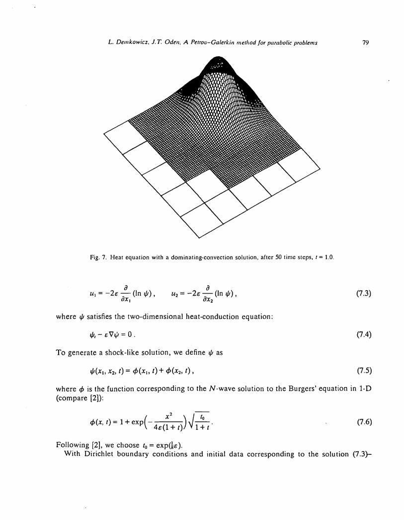
Fig. 7. Heal equation with a dominating-convection solution, after 50 time steps, t = 1.0.

79

au. = -2£ - (In I/J),ax.

(7.3)

where I/J satisfies the two-dimensional heat-conduction equation:

I/J, - E V ~I = 0 .

To generate a shock-like solution, we define I/J as

(7.4)

(7.5)

where c/> is the function corresponding to the N-wave solution to the Burgers' equation in I-D(compare [2]):

(7.6)

Following [21. we choose to = exp(~E).With Dirichlet boundary conditions and initial data corresponding to the solution (7.3)-

80

Fig. 8. Heat equation with a dominating-convection solution. after 75 time steps, t = 1.5.

Fig. 9. Heat equation with a dominating-convection solution, after 100 time steps. t = 2.0.

L. Demkowicz, J.T Oden. A Petrou-Galerkill method for parabolic problems

Fig. 10. Burgers' equations, first component of the solution after 1 time step, t = 0.02.

HI

(7.6), problems (5.1) has been solved in a square domain n = (0, 1) x (0, 1) with the followingnumerical data:

E = 0.004,

number of superelements = 5 x 5 ,

8 = 0.001 (compare (6.1))

TaL = 0.002,

~t=0.02.

82 L. Demkowicz, J.T Odell, A Petrov-Galerkin method for parabolic problems

Fig. 11. Burgers' equations, second component of the solution after 1 time step, t = 0.02.

Of the three methods of constructing characteristics (5.4), we have tested the second one-theimplicit scheme with a local solution to (5.3) by the Newton-Raphson technique. With atolerance TOLCONV == 0.001, the number of iterations required never exceeded 2. Figs. 10and 11 present two components of u after the first iteration at t = 0.02. Due to the symmetryof the exact solution,

(7.7)

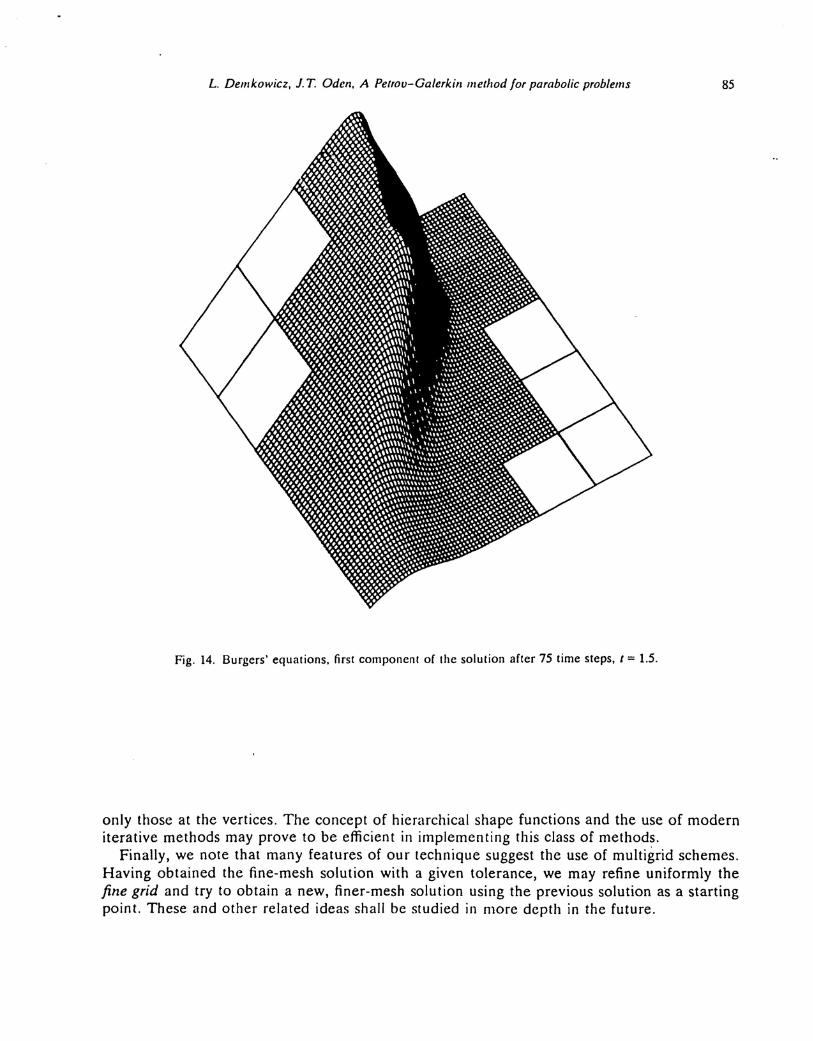
preserved by our numerical scheme, it is sufficient to present the results for only one of thecomponents. Thus, Figs. 12, 13 and 14 show the development of the first component u, after25, 50 and 75 iterations, i.e., at the time t = 0.5, 1.0 and 1.5. Finally, Fig. 15 presents the meshfor the first component u" after 50 iterations, at t = 1 with the corresponding local errors anderror estimates.

L. Demkowicz, 1. T. Oden, A Petrov-Galerkin method for parabolic problems

Fig. 12. Burgers' equations, first component of the solution after 25 time steps, t =: 0.5.

8. Concluding remarks

83

The key to the generalization of our method, described in [2], to multi-dimensional cases isthe concept of a 'semi-exact' (fine-grid) solution and the use of 'numerically optimal' testfunctions. Accepting the fine-mesh solution also proved to be useful in ensuring L2-stability, asis already the one-dimensional case. The fine-mesh solution proved to be easy to implementusing the numerically optimal test function for the transport problem. For purely elliptic

84 L. Demkowicz, J.T Odell, A Petrov-Galerkill method for parabolic problems

Fig. 13. Burgers' equations, first componcnt of thc solution after 50 time steps, t = 1.0.

problems, other methods for approximation of the optimal test functions suggest themselves.For example, hierarchical, p-version finite element methods could be employed to produce asemi-exact solution obtained with a high-order polynomial approximation. The correspondingPetrov-Galerkin scheme would have the property that the internal degrees of freedom of eachsuperelement would be eliminated.

Among possible directions for further development, we mention that for our Petrov-Galerkin scheme we were able to eliminate all the 'internal' degrees of freedom in superele-ments. It is not clear if it would be possible to adaptively discard interelement nodes, leaving

L. Demkowicz, J. T Oden, A PetfOv-Galerkin method for parabolic problems

Fig. 14. Burgers' equations, first component of the solution after 75 time steps, t = 1.5.

85

only those at the vertices. The concept of hierarchical shape functions and the use of moderniterative methods may prove to be efficient in implementing this class of methods.

Finally, we note that many features of our technique suggest the use of multigrid schemes.Having obtained the fine-mesh solution with a given tolerance, we may refine uniformly thefine grid and try to obtain a new, finer-mesh solution using the previous solution as a startingpoint. These and other related ideas shall be studied in more depth in the future.

86 L. Demkowicz, J.T Oden, A Petrou-Galerkill method for parabolic problems

L2_ Error Estimate2

I.- Error

L00 -Error

O.783(E-3) 0.782(E-3) ::0.228(E-5) 1).166(E-4) 0.645(E ..1) : 0.318(E-2) 0.440(E-4)

0.313(E-4) 0.204 (E-3) 0.117(E-1) : 0.34I.(E-1) 0.493(E-3)-.,-,. . ., .,.

O.783(E-3)

0.361(E-5) 0.287 (E-4) 0.106(E-2) 0.308(E-2) 0.362(E-4)

0.375(E-4) 0.608(F.-3) 0.171(E-1) 0.345(E-1) 0.417(E-3), . , ,

, '- .' , I 1-1

0.904 (E-5)0.196(E-4) 0.373(E-3) 0.103(E-2) 0.543 (E-3) 0.676(E-5)

0.666(E-3) 0.535(F.-2) 0.10!l(E-1) 0.896(E-2) 0.150(E-3)

f-.. ." ..

f.' '" U.L..u.....LJ, I I I I

0.985(E-Ii)0.118(E-3) 0.373(F.-3) 0.38R(E-3) 0.182(E-4) 0.164(£-5)0.157(£-2) 0.400(1':-2) 0.543(1':-2) 0.664(1':-3) 0.215(1':-4)

,''' ,-on , , , . ...; "T -, , " I

. 0.189(E-5) 0.518(E-6)

0.487 (E-4) 0.847(£-4) 0.276(E-4) 0.255(E-5) 0.452(E-6)

0.727(E-3) 0.127(1':-2) 0.812(1':-3) t'.'28(E-4) 0.699(F-5)

. , tf±.H-i

Fig. 15. Burgers' equations, the optimal mesh for the first component with the local L2-errors and L2-errorestimates after 50 time steps, t = 1.0.

References

[1] l.W. Barrett and K.W. Morton, Approximate symmetrization and Petrov-Galerkin methods for diffusion-convection problems, Compul. Meths. App!. Mech. Engrg. 45 (1984) 97-122.

[2) L. Demkowicz and J.T. Oden, An adaptive characteristic Petrov-Galerkin finite element method for con-vection-dominated linear and non-linear parabolic problems in one space variable, TICOM Rep!. 85-3, TheUniversity of Texas at Austin, April 1985.

[3] l. Donea, S. Giuliani, H. Laval and L Quartapelle. Time-accurate solution of advection-diffusion problems byfinite elements, Compul. Meths. App!. Mech. Engrg. 45 (1984) 123-145.

L. Demkowicz. J. T Oden, A Petrov-Galerkin method for parabolic problems 87

[4J J. Douglas and T.F. Russell, Numerical methods for convection-dominated diffusion problems based oncombining the method of characteristics with finite element or finite difference proccdures, SIAM J. Numer.Anal. 19 (5) (1982) 871-885.

[51 C. Flelcher. Thc Galcrkin Method and Burgcrs' equation. in: J. Noye, ed., Computational Techniques forDifferential Equalions (North-Holland, Amslerdam, 1984) 355-475.

[6J J. M. Ortega, Numerical Analysis, A Second Course (Academic Press, New York, 1972).[7] O. Pironneau, On the transport-diffusion algorithm and its applications to Navier-Stokes equations, Numer.

Math. 38 (1982) 309-332.