use of air cooling and its effectiveness in dry machining
TRANSCRIPT

Department of Mechanical Engineering
Use of Air Cooling and its Effectiveness in Dry Machining Processes
Brian Boswell
This thesis is presented for the degree of Doctor of Philosophy
of Curtin University of Technology
June 2008

ii
CANDIDATE STATEMENT
To the best of my knowledge and belief this thesis contains no material previously
published by any other person except where due acknowledgement has been made.
This thesis contains no material which has been accepted for the award of any other
degree or diploma in any university.

iii
ABSTRACT
Traditional liquid coolants used in metal machining are known to contain chemical carcinogens that could present serious health risks for machine operators and have inherent waste disposal concerns on the environment. In lessening these adverse effects, the manufacturing industry continually seeks to develop machining techniques incorporating liquid-less (dry) methods or environmentally benign coolants. Air-jet cooling is widely regarded as a viable alternative for liquid coolants in machining processes. This thesis proposes a novel air jet cooling arrangement, and assesses its thermal effectiveness and operational compatibility for specific requirements in metal cutting operation. For tests, steel rods were machined on a standard lathe workbench at selected cutting depth, feed and speed. Type 1040 steel, which is commonly used in automobile industry, was chosen as work piece material. Instead of traditional liquid coolant, a specially designed compressed air jet is used to dissipate heat generation in the cutting zone at the tool tip. The tool tip is presented orthogonally to the work piece to maintain conformity with relevant established cutting tool theories. A special air jet configuration based on a Ranque-Hilsch vortex tube was designed and developed for cooling the cutting zone and tool tip. The tool tip temperatures were measured by installing thermocouples at strategic locations on the tool piece and recorded on a data-logger for a range of cutting depths, feeds and speeds. The cutting power was measured with a power meter attached to the electrical power supply to the lathe. For comparison purposes, tests were also conducted with conventional single-nozzle air jets in place of the vortex-tube jets, using traditional liquid coolant and without any cooling applied to the tool tip. A thermal vision camera was also deployed for selected tests to ascertain the temperature characteristics at the tool tip. The data was analysed to establish the thermal characteristics at the tool tip with vortex tube air jet, conventional air jet and no air jet cooling. The measured temperatures and cutting data were used to make assessments on cooling efficiency of jets used and surface finish quality of work piece. Estimates of tool life were made from the cutting theory to determine the effectiveness of the cooling systems used in the machining process. It is found that the proposed vortex tube based air jet cooling arrangement provides a highly efficient heat removal mechanism for metal cutting and delivers thermal cooling performance very much comparable to traditional liquid coolants without the inherent chemical exposure risks to machine operators and harmful impact on the environment. With the proposed air jet cooling, the tool life is very much unchanged and the surface finish quality of work piece shows no significant change while savings will realise though lesser dependency on liquid coolant requiring careful disposal and associated costs.

iv
ACKNOWLEDGEMENTS
The author gratefully acknowledges the assistance of the following people:
Associate Professor Tilak T Chandratilleke for all his guidance and help during the
many years taken to complete this research;
Dr Ian Davies whose advice on writing this thesis was most appreciated;
The Mechanical Engineering Department technicians for their assistance during the
many hours of testing and manufacturing of test equipment used is this research.
Finally, I especially thank my wife Marion Boswell without whose encouragement
and help this thesis would never have been completed.

v
CONTENTS
TITLE............................................................................................................................ i
CANDIDATE STATEMENT ................................................................................... ii
ABSTRACT................................................................................................................iii
ACKNOWLEDGEMENTS........................................................................................ iv
CONTENTS................................................................................................................. v
APPENDIX………………………………………………………………………...viii
LIST OF FIGURES…………………………………………………………..……...ix
LIST OF TABLES…………………………………………………………………..xii
NOTATION………………………………………………………………………...xiii
CHAPTER 1 INTRODUCTION ................................................................................. 1
1.1 Overview Of The Machining Process.......................................................... 1
1.2 Machining Process ....................................................................................... 1
1.2.1 Metal cutting chip formation................................................................ 1
1.2.2 Metal cutting ........................................................................................ 3
1.3 Generalisation Of Tool Life ......................................................................... 5
1.4 Tool Tip Heat Generation ............................................................................ 6
1.5 Environmental Cost Of Liquid Coolant ....................................................... 7
1.6 Coated Tungsten Tool Tips.......................................................................... 8
1.7 Objective of Research .................................................................................. 9
CHAPTER 2 REVIEW OF PREVIOUS WORK - MACHINE TOOL COOLING . 10
2.1 Introduction................................................................................................ 10
2.2 Mechanics Of Metal Cutting...................................................................... 10
2.2.1 Cutting theory .................................................................................... 10
2.2.2 Heat generated by plastic deformation and friction ........................... 14
2.3 The Effect Of Coolant On Tool Performance............................................ 19
2.3.1 Traditional liquid coolant................................................................... 19
2.3.2 Environmental concerns of using coolant .......................................... 22
2.4 Alternative Methods To Liquid Coolant .................................................... 23
2.4.1 Dry machining.................................................................................... 23

vi
2.4.2 Minimum quantity lubricant (MQL).................................................. 28
2.4.3 High pressure jet-assisted cooling...................................................... 31
2.4.4 Cryogenic cooling .............................................................................. 33
CHAPTER 3 TOOL LIFE ......................................................................................... 38
3.1 Introduction To Tool Life .......................................................................... 38
3.2 Tool Life Analysis...................................................................................... 39
3.2.1 Empirical tool life relationships......................................................... 39
3.2.2 Tool life and wear mechanisms.......................................................... 43
3.2.3 Temperature dependency on tool life................................................. 48
3.2.4 Tool Wear Rates.................................................................................55
3.3 Concluding Remarks.................................................................................. 60
CHAPTER 4 CHARACTERISTICS OF AIR COOLING........................................ 62
4.1 Overview Air Cooling................................................................................ 62
4.2 Jet Impingement Cooling Process.............................................................. 64
4.2.1 Introduction........................................................................................ 64
4.2.2 Jet impingement cooling mechanism................................................. 64
4.3 Ranque-Hilsch Vortex Tube ...................................................................... 70
4.3.1 Introduction to Ranque-Hilsch vortex tube........................................ 70
4.3.2 Vortex tube energy transfer process................................................... 72
4.4 First Law Of Thermodynamics Implications In Vortex Tube ................... 76
4.4.1 First Law analysis ..............................................................................76
4.4.2 Temperature separation...................................................................... 79
4.4.3 Transfer of vortex tube temperature by energy method..................... 81
4.4.4 Vortex tube efficiency........................................................................ 83
4.5 Vortex Cooling Effect ................................................................................ 86
4.5.1 Elements of the vortex tube................................................................ 86
4.5.2 Experimental analysis on vortex tube configurations ........................ 88
4.5.3 Experimental data and analysis.......................................................... 92
CHAPTER 5 TOOL TIP TEMPERATURE MEASUREMENT ............................ 101
5.1 Overview.................................................................................................. 101

vii
5.2 Temperature Measurement Methods........................................................ 102
5.2.1 Thermo-chemical ............................................................................. 102
5.2.2 Radiation thermometry technique.................................................... 104
5.2.3 Thermo-electrical techniques........................................................... 117
5.2.4 Indirect measurement of tool interface temperature ........................ 120
5.3 Tool Tip Temperature Measurement ....................................................... 121
5.3.1 Thermocouple method ..................................................................... 121
5.3.2 Machining tests ................................................................................ 124
5.4 Discussion ................................................................................................ 127
CHAPTER 6 AIR-COOLING OF TOOL INTERFACE ........................................ 130
6.1 Overview Of Cooling Tool Cutting Zone ................................................ 130
6.2 Impingement Cooling During Metal Cutting........................................... 131
6.2.1 Experimental impingement configuration ....................................... 131
6.2.2 Impingement cooling tests ............................................................... 134
6.2.3 Tool tip temperature - impingement cooling ................................... 136
6.3 Vortex Tube Cooling During Metal Cutting............................................ 147
6.3.1 Tool tip temperature during vortex tube air-cooling........................ 147
6.3.2 Chip breaker air jet cooling.............................................................. 153
6.4 Tool Life................................................................................................... 159
6.4.1 Effect of air-cooling on tool life....................................................... 159
6.4.2 Discussion ........................................................................................ 162
CHAPTER 7 CONCLUSIONS................................................................................ 165
7.1 Introduction.............................................................................................. 165
7.2 Significance And Outcomes..................................................................... 165
7.3 Recommendations And Possible Further Developments......................... 166
7.4 Conclusion ............................................................................................... 167
REFERENCES......................................................................................................... 168

viii
APPENDIX
Appendix A
Parameters Investigated To Obtain The Optimum Vortex Tube…………………. 177
Appendix B
Thermoelectric Voltages Used For Calibration……………………………...…….180
Appendix C
Impingement Jet Nozzle Test………………………………………..……………181
Appendix D
Vortex Tube Jet Nozzle Test……………………………………………………….183
Appendix E
Typical Temperatures Recorded During Machining……………………………...184
Appendix F
Publications and Conference Presentations ……………………………………….188

ix
LIST OF FIGURES
Figure 1.1: Discontinuous chip .................................................................................... 2
Figure 1.2: Continuous chip......................................................................................... 2
Figure 1.3: Continuous chip with built up edge........................................................... 3
Figure 1.4: Metal removal by oblique turning process. ............................................... 3
Figure 1.5: Metal cutting configuration needed for orthogonal machining. ................ 4
Figure 1.6: Special cutting conditions needed on a lathe to obtain orthogonal
machining..................................................................................................................... 5
Figure 1.7: Temperatures at shear plane AB................................................................ 6
Figure 1.8: Typical materials used to produce tip insert. .............................................8
Figure 2.1: Shear plane model of chip formation ...................................................... 11
Figure 2.2: Actual plastic shear zone of chip formation ............................................ 11
Figure 2.3: Shear plane model of chip formation showing force and velocity. ......... 12
Figure 2.4: Block slip model for total shear strain of chip formation........................ 13
Figure 2.5: Heat generating areas in chip................................................................... 15
Figure 2.6: Tool tip cooled by traditional cutting fluid..............................................20
Figure 2.7: Traditional cutting fluid showing not reaching the tool tip interface. ..... 20
Figure 2.8: Volume of material removal per tool life for a depth of cut of 1mm...... 24
Figure 2.9: Volume of metal removed for 0.3 mm flank wear. ................................. 24
Figure 2.10: Flank wear (VBb) volume of metal removed........................................ 25
Figure 2.11: Arrow “A” identifies flank face wear on the tool tip. ........................... 26
Figure 2.12: Flank wear (VBB) volume of metal removed. ...................................... 26
Figure 2.13: Surface roughness (Ry) for all conditions. ............................................ 27
Figure 2.14: Tool life in volume of chip removed..................................................... 28
Figure 2.15: Temperature comparison of MQL and wet and dry turning.................. 29

x
Figure 2.16: Variation of cutting temperature during MQL, wet and dry turning..... 29
Figure 2.17: Surface roughness during MQL, wet and dry turning. .......................... 30
Figure 2.18:Variation of surface roughness during MQL, wet and dry turning. ....... 31
Figure 2.19: Diagram of a vapour generator device and vapour feeding system. ..... 32
Figure 2.20: The cutting temperature comparison of dry, compressed air, oil and
emulsion and water vapour. ....................................................................................... 32
Figure 2.21: The surface roughness comparison of dry, compressed air, oil and
emulsion and water vapour. ....................................................................................... 33
Figure 2.22: Tool tip cooled by nitrogen chamber positioned under the tool tip. ..... 34
Figure 2.23: Isothermal contour for dry cutting......................................................... 35
Figure 2.24: Isothermal contour for wet cutting. ....................................................... 35
Figure 2.25: Isothermal contour for workpiece precooling. ...................................... 36
Figure 2.26: Isothermal contour for tool back cooling. ............................................. 36
Figure 2.27: Isothermal contour for liquid nitrogen sprayed on tool face. ................ 37
Figure 2.28: Tool temperature verses cutting speed.................................................. 37
Figure 3.1:Typical crater and flank wear on lathe tools............................................. 39
Figure 3.2: The chip equivalent. ................................................................................ 41
Figure 3.3: Relationship between the specific wear rate and tool temperature. ........ 45
Figure 3.4(a-c): Tool wear and tool life data as functions of the measured cutting
temperature when machining stainless steel with carbide tools................................. 48
Figure 3.5(a-c): Predicted and experimental tool life results..................................... 51
Figure 3.6(a-d):Tool life cutting times for various cutting speeds and undeformed
chip thickness. ............................................................................................................ 53
Figure 3.7:Tool data of (Figure 3.6) plotted as a function of the predicted cutting
temperature from Bruce. ............................................................................................ 54
Figure 3.8: Predicted and experimental tool life for machining ................................ 55

xi
Figure 3.9: Results of wear rate against reciprocal of tool temperature for two rake
angles.......................................................................................................................... 57
Figure 3.10: Wear rate for two tool materials when machining axle steel of 0.41
percent carbon content. .............................................................................................. 58
Figure 3.11: Wear rates for two work materials when machining with K45 material.
.................................................................................................................................... 59
Figure 4.1: Flow regions for air impinging free-surface jet....................................... 65
Figure 4.2: Flow regions for air impinging jet on the top face of a tool tip............... 66
Figure 4.3: Laminar Boundary Layer......................................................................... 66
Figure 4.4: Visualised flow of an impinging jet. ....................................................... 67
Figure 4.5: Simplified flow contour and velocity profile of an impinging jet. .......... 68
Figure 4.6: Variation of Nusselt number on a flat plate during jet impingement. ..... 69
Figure 4.79: Temperature decrease at cold exit with respect to tube length.............. 96
Figure 4.80: Temperature increase at hot exit with respect to tube length. ............... 97
Figure 5.13: Temperatures found by using imbedded thermocouples. .................... 117
Figure 6.1: Thermocouples channel positions in tool tip......................................... 131
Figure 6.2: Temperature for wet and dry machining. .............................................. 131

xii
LIST OF TABLES
Table 2.1: Influence of various cutting fluids on the tool chip interface………...….13
Table 4.1: Single jet nozzle……………….……………………………………...….61
Table 4.2: 1 mm diameter multi-hole jet nozzle…………………………………….61
Table 4.3: Three jet nozzle ……………………………………………………….…62
Table 4.4: 2 mm diameter angled nozzle ……………………………………...……62
Table 4.5: Vortex test parameters …………………………………………………..83
Table 4.6: Vortex tube optimum configuration …………………………………….83
Table 4.7: Recorded readings from test …………………………………………….86
Table 5.1: Cutting conditions used during power readings ……………………….119
Table B.1: Sample of thermoelectric voltages for type K thermocouple …………172

xiii
NOTATION
friction surface area A1 mm2
vortex cold nozzle area A m2
constant a1
constant a2
chip cross sectional area Ao mm2
constant b
constant c
cost C
specific heat capacity cp
constant Ct
depth of cut d mm
jet diameter D mm
bar diameter D1 mm
machine diameter D2 mm
constant E1
friction force F kN
feed rate f m/min
cutting force Fc kN
force perpendicular to cutting velocity Ff kN
percentage of full load FL
normal force on the shear plane AB Fn kN
shear force Fs kN
frequency fs
nozzle tool tip gap G mm
contact length h mm
air enthalpy ha kJ/s
crater wear depth hc mm
thermal conductivity K W/m K
kinetic energy KE kJ
tool life cutting time L min.
latent heat evaporation Le kJ/kg
cutting edge length le mm

xiv
rubbing distance l f mm
mass m
mass of cutting fluid mcf
motor efficiency ME
motor load MP kW
normal force at tool tip N kN
number of shocks ns
Nusselt number Nu
operating hours OH hr
tool pressure p N/mm2
air pressure P MPa
volumetric specific heat ρc J/cm3 oC
potential energy PE kJ
heat quantity Q
chip equivalent q
resultant force R kN
radial distance from centre of jet r mm
ideal gas constant R
chip ratio rc
Reynolds number Re
tool nose radius rε mm
thermal number RT
surface roughness Ry µm
specific heat of material S J/kg K
system entropy S kJ
cutting distance Scd mm
tool temperature T K
feed/rev. t1 mm/rev
chip thickness t2 mm
absolute temperature Ta K
temperature rise in the shear zone TAB oC
mean temperature rise of chip Tc oC
cold air exit temperature Tc oC
temperature of the friction surface Tf oC

xv
tool flank Tflank K
hot air exit temperature Th oC
air inlet temperature Ti oC
interface temperature Tint oC
maximum rise at tool chip interface Tm oC
mean chip interface temperature Ts oC
shear zone temperature Tsz oC
tool thermocouple temperature Tth K
tool temperature Ttool K
work temperature Tw oC
system internal energy U kJ
specific energy during cutting Uc J/m3
cutting velocity V m/s
air velocity Va m/s
spindle speed N rpm
flank wear VBb mm3
chip velocity Vc m/s
shear velocity Vs m/s
chip width w mm
tool wear W
wear rate due to abrasion Wa
wear rate due to brittle fracture Wb
wear rate due to other mechanism Wi
wear rate due to rate processes Wr
wear rate ws
adjusted wear rate ws1
distance between air stream z m
mass flow rate m& kg/s
heat flow rate Q& kJ/s
system work W& kJ/s
rake angle α deg
abrasive resistance of the tool σa
resistance to brittle fracture σs

xvi
thermal diffusivity αt mm2/s
average shear plane temperature β oC
shear strain γ
heat conducted into the work ҝ W/m K
friction angle λ deg
friction co-efficient µ
cold fraction µcf
density of the work material ρ kg/m3
volumetric specific heat ρc J/cm3 oC
side cutting edge σ deg
abrasive resistance of the tool σa
resistance to brittle fracture σs
shear strength of the work material τ MN/m2
shear angle φ deg
tool sharpness ψT

CHAPTER 1: INTRODUCTION
1
CHAPTER 1
INTRODUCTION
1.1 Overview Of The Machining Process
Since the beginning of the industrial revolution metal cutting manufacturing
processes have involved the removal of unwanted material. Metal removal continues
to be the principal method of manufacturing. The advent of rapid prototyping
machines capable of producing the most complicated of shapes still does not reduce
the volume of machining necessary today. Interestingly, in 1971, the Delphi Type
Forecast [1] for the International Institution for Production Engineering predicted
that machining would remain the principal method of metal product manufacturing.
The popularity of machining throughout the world however ignores one major
problem: the enormous amounts of liquid cutting fluid needed to prolong tool life
gives rise to serious environmental issues as well as health concerns for the machine
operators. Being aware of this, manufacturers worldwide have been trying to
minimise or eliminate the use of liquid coolant during metal cutting. This has given
rise to manufacturers incorporating a limited amount of dry machining into the
manufacturing processes. The aeronautical industry relies on dry machining for most
of its metal cutting processes due to the machinability of lighter and softer materials.
On the other hand the automotive industry is desperate to achieve dry machining for
economic and environmental (green manufacturing) reasons. Unfortunately, the
materials used in this particular industry are harder and tougher, and are not as easy
to machine as aluminium alloys used in the aerospace industry. A brief history of the
metal cutting process and its investigation can be found in ‘The Mechanics of
Machining” by Armarego and Brown [2], and a more detailed review in an article by
Finnie [3].
1.2 Machining Process
1.2.1 Metal cutting chip formation
Fundamentally, machining is a material removal process where a layer of material is
removed in the form of chips from the workpiece by the action of a wedged shaped

CHAPTER 1: INTRODUCTION
2
cutting tool. The first studies of chip formation were qualitative in nature and
investigated the material flow (deformation) in the chip formation. Rosehain and
Sturney [4] attempted to classify the process according to the type of chip produced.
These authors classified the chip as “shear”, “tear”, and “flow chips”. This
classification was used until 1938 when Ernes [5] presented his classical observation
of chip formation. They were:
(a) Discontinuous Chip
Figure 1.1 shows a segmented discontinuous chip, which exhibits some
deformation even though it is broken at fairly regular intervals by fracture
across the width and thickness of the chip. The associated machine surface is
rough and irregular.
Figure 1.1: Discontinuous chip
Shown in Figure 1.2 is a continuous chip. As the name suggests, the chip is
formed as a continuous ribbon when machining ductile materials under ideal
cutting conditions. This chip is the result of continuous plastic deformation
leading to steady cutting forces and a smooth machined surface.
Figure 1.2: Continuous chip

CHAPTER 1: INTRODUCTION
3
(b) Continuous Chip with Built-up Edge
This type of chip is formed when machining ductile materials under certain
cutting conditions, and is shown in Figure 1.3. The chip is continuous, but at
the cutting edge on the tool face there is a build up of deformed material.
Ernest [5] was also able to show that the build up and breakdown of this
deformed material was cyclic in nature. The breakdown was such that part of
the build-up material attached itself to the machined surface, while the other
part attached itself to the back of the chip. Due to the short cycle time the
associated machined surface is rough and irregular.
Figure 1.3: Continuous chip with built up edge.
1.2.2 Metal cutting
The normal and most common metal cutting condition is known as oblique
machining, which is the cutting process when turning, milling and drilling. Figure
1.4 shows metal being removed by a typical oblique turning process.
V = cutting speed, d = depth of cut, w = chip width, t2 = chip thickness, t1 = feed/rev, N = spindle
speed, σ = side cutting edge, D1 = bar dia, D2 = machined dia.
Figure 1.4: Metal removal by oblique turning process.

CHAPTER 1: INTRODUCTION
4
Oblique machining is a complex machining process due to the shape of the cutting
edge. Attempts have been made to analyse the process Lin and Oxley [6], although
this results in a complex solution to analyse. Figure 1.5 shows a simplified metal
cutting process known as orthogonal machining. The orthogonal cutting process is
normally the analysis used by researchers as it eliminates a number of variables that
can affect the cutting theory. For this reason the orthogonal model is used for the
analysis of the machining process in this research.
Figure 1.5: Metal cutting configuration needed for orthogonal machining.
In orthogonal machining the cutting edge of the tool is set perpendicular to the
direction of the cutting, and parallel to the surface being machined, as shown in
Figure 1.5 and 1.6. Also, the tool must overlap the cutting surface such that the metal
removal is only done on the primary surface. If the width of cut is very much larger
than the depth of cut shown in Figure 1.5 t1 < w, then the flow of the material
approximates to that of plane strain: that is the flow is in two directions only.

CHAPTER 1: INTRODUCTION
5
Figure 1.6: Special cutting conditions needed on a lathe to obtain orthogonal
machining.
Under certain conditions on the lathe the machining processes can be considered as
approximately orthogonal. These conditions are that the feed must be small relative
to the depth of cut - making most of the cutting taking place in the direction of the
feed, and the cutting on the nose of the tool will be negligible (Mikell P. Groover
[7]). The special machining conditions that allow orthogonal analysis to be used were
employed in determining the set feed rate and depth of cut on the engine lathe.
1.3 Generalisation Of Tool Life
Information available for establishing tool life is largely generalised and empirical in
nature. This is fundamentally due to the cutting process, as the changing of one
parameter will result in a new set of data. For example, the classification of material
and processes in the Machining Data Handbook [8] is wide and varied. When
considering low carbon steels, it is noted that as many as twenty different steels are
found in that group, and suggests cutting conditions for different operations are only
in the form of “first try” conditions. Such data can in fact have a variability of as
much as 50 percent to 100 percent. Also, the tool life expected is stated at 30 to 60
minutes for a throw-away carbide tool tip for continuous cutting. This is in fact
another generalisation because there is also great variability in the shape/type of tips
and grades of tips. Just how large is the variability cannot be estimated; that in turn
reduces the reliability of the available data.

CHAPTER 1: INTRODUCTION
6
In order to overcome these difficulties and provide more reliable data, many
countries have set up Machining Data Banks [9] based on information on the
machining process collected from various sources. In conjunction with this available
machining data, it is apparent that appropriate tool life tests need to be carried out for
the material and tool tips used in this research. This will allow this research to
determine the effectiveness of air-cooling of the tool tip, by comparing air-cooling
test data against reliable tool life data.
1.4 Tool Tip Heat Generation
Manufacturers know that the hotter the tool becomes the quicker the tool tip will
break down and need to be replaced. Clearly it is essential for modern manufacturing
to prolong tool life to maximise production. The main parameters that are known to
have influence on the tool tip temperature are the tool tip material, the material being
cut, and the cutting velocity. Figure 1.7 shows typical temperatures that can be
generated in the cutting zone. As the yield strength of the material is approached, the
heat helps the separation of the chip from the work piece.
(obtained from G. Bothroyd) [10]
Figure 1.7: Temperatures at shear plane AB.

CHAPTER 1: INTRODUCTION
7
The more heat in the primary cutting zone the easier the chip will separate. However,
with too much heat the tool tip material will also want to separate from the tool tip,
vastly reducing its tool life. Traditionally, the approach to prolong tool life is to
supply large amounts of liquid cutting fluid to the cutting zone to cool the tool tip.
The consequence of this is to add additional cost to the product, and appropriate
costly disposal preparations must be in place for the contaminated cutting fluid.
Therefore, exploiting the potential of dry machining is economical and
environmentally necessary for modern manufacturing.
1.5 Environmental Cost Of Liquid Coolant
Manufacturing industries in industrial nations throughout the world are now both
coerced by government legislation and the growing awareness of society to ensure
that their manufacturing processes do not harm the environment. For this reason
increased attention is now paid to the environment and health impact of industry
activities. In the case of the metal cutting process, manufacturers are encouraged to
find ways to reduce the use of liquid coolant during machining. Over the years other
methods of cooling the tool tip have been tried with some degree of success. CO2 was
used in the mid-nineteen fifties and hailed as the greatest solution to the cooling of
tool tips. However, it was soon discovered by those companies who adopted this
method of cooling to be expensive and relied on a large amount of auxiliary
equipment. Today this method of cooling would not be considered on environmental
grounds, as CO2 is a “greenhouse gas”, and would promote this phenomenon. In
more recent times, the use of cryogenic cooling has been used with some success, but
this method also depends on large amounts of auxiliary equipment available to
supply the liquid nitrogen, and this is expensive to use. In addition the machine tool
operators safety is of concern, as care must be taken in using this very cold fluid.
As more attention is being focused on the role of cutting fluids in machining, there is
a new ISO 14000 international environmental management system standard to guide
manufacturers. The aim here is to help manufacturers reduce the environmental
burden produced by manufacturing. An environmental burden analysed by H. Narita
et al. [11] that considers all aspects of the machining process shows that liquid
coolant alone contributes to 0.98 kg-CO2/L equivalent CO2 emission intensities. This
is the amount of greenhouse gas that has been produced during the making of the

CHAPTER 1: INTRODUCTION
8
liquid coolant and from using it. So the machine tool energy efficiency and the
impact of the process waste have a negative effect on the environment D. Dudzinski
[12]. These CO2 emission values clearly show why dry machining is being
considered more and more for applicable machining processes.
1.6 Coated Tungsten Tool Tips
Recent advances in tool tip coatings have proven to be most effective in improving
the performance of dry cutting by reducing the ability of the cut material to stick to
the tool tip. Figure 1.8 shows a tungsten coated tool tip with three layers. This tool
tip has outstanding wear resistance and toughness and is:
• suitable for fast and dry machining;
• suitable for mass and large batch production;
• suitable for unmanned machining.
(Picture from Seco web site on the 6th Dec. 2005) http://www.secotools.com/template/start
Figure 1.8: Typical materials used to produce tip insert.
However, even with the improvements to tool tip materials, tool life will always be
reduced due to the higher working temperatures of dry machining K. Causton [13].
As previously outlined, the use of dry machining can be considered as a “green”
manufacturing process as there is no pollution generated waste with the cutting of the
material. The significance of using dry machining can be highlighted when we note
that, in Australia alone, millions of litres of liquid coolant are consumed each year.
This has been estimated to constitute about 7 to 17 percent of the total machining

CHAPTER 1: INTRODUCTION
9
costs. The equivalent CO2 emissions contributed by the disposal of the liquid coolant
can be evaluated as 0.192 kg-CO2/L. Research has shown that dry machining is
preferably carried out at high speed N.A. Abukhshim et al. [14]. Although cutting
metal at high speeds is associated with high temperatures, most of the additional heat
generated is removed by the chips.
1.7 Objective of Research
The object of this research is to show that dry machining with air-cooling can be
shown to be as effective as - if not better than - traditional wet machining of metals.
Dry machining alone eliminates the use of coolant and the waste burden on the
environment, therefore reducing machining costs. Unfortunately, dry machining by
itself reduces the life expectancy of the cutting tool due to the high temperatures
involved in machining. Dry machining with the addition of air-cooling extends tool
life during machining. Air-cooling reduces the temperature at the tool interface, it is
readily available and environmentally friendly, it is easy to work with, and it is also
cost effective. However, just applying a jet of air does not simply provide the
solution. The challenge is to ensure that air-cooling can be made to be as effective as
traditional wet machining methods of cooling the tool tip during machining. Also,
the performance of the air-cutting process should not produce an inferior surface
finish in comparison to one produced by traditional coolant.

CHAPTER 2: REVIEW OF PREVIOUS WORK – MACHINE TOOL COOLING
10
CHAPTER 2
REVIEW OF PREVIOUS WORK - MACHINE TOOL COOLING
2.1 Introduction
Metal cutting theory and tool cooling approaches are presented in this literature
review to obtain a sound understanding of the metal cutting process. From the
analysis of these theories the most important parameters are identified that affect the
tool tips performance. The major detrimental parameter to the tool performance is the
generation of heat at the tool interface. This increased temperature at the tool
interface has proved to have an enormous effect on the wear mechanisms. To reduce
the wear on tool tips it is essential to dissipate the generated heat at the cutting zone.
An understanding of how the heat is generated and what affects it has on the tool tip
is essential in any development of an efficient new air-cooling system for the tool tip.
Measuring meaningful tool tip temperature during machining has always been
extremely difficult. An attractive alternative approach has been the development of
mathematical models that enable you to calculate the tool tip temperature. The earlier
analytical work on steady-state temperatures generated during metal cutting was
developed by Chao and Trigger [15], although there are other analytical models
including the model by Boothroyd [10] as modified by Oxley [16].
2.2 Mechanics Of Metal Cutting
2.2.1 Cutting theory
Most analytical studies of chip formation have been restricted to continuous chip
formation due to the steady state conditions under which the chip is formed. The type
of chips that were formed during the experimental tests in this research were all of
this type. Based on observations of the chip formation process, Ernst [17] derived the
geometrical configuration as shown in Figure 2.1, resulting in the shear plane model
for the chip formation.

CHAPTER 2: REVIEW OF PREVIOUS WORK – MACHINE TOOL COOLING
11
Figure 2.1: Shear plane model of chip formation
However, it has long been known that the actual process of chip formation is in two
separate shear zones Christopherson et al [18]: a primary shear zone in front of the
tool, and a secondary deformation zone at the tool chip interface as shown in Figure
2.2. Ernest derived the model by neglecting the secondary deformation zone and
idealising the primary shear zone by a plane.
Figure 2.2: Actual plastic shear zone of chip formation
It also assumes that the tool is perfectly sharp and the chip curl is neglected. The chip
is assumed to be formed by simple shear on a shear plane “AB”, as shown in Figure
2.3 which is at the shear angle, φ, to the cutting velocity, V. The shear angle is the
defining parameter for the geometry of the shear plane model. The model assumes
that the work material approaches “AB” with the cutting velocity. This implies a
discontinuity in the tangential velocity along “AB” called the shear velocity, Vs,
which is acceptable as only the velocity normal to “AB” must be continuous.

CHAPTER 2: REVIEW OF PREVIOUS WORK – MACHINE TOOL COOLING
12
Figure 2.3: Shear plane model of chip formation showing force and velocity.
From Figure 2.3 it is observed that the cutting velocity, shear velocity and chip
velocity, Vc, can be related by the equations (2.1) and (2.2) obtained from Altintas
[19]:
)cos(
sin
αφφ
−= V
Vc (2.1)
)cos(
cos
αφα
−= V
Vs (2.2)

CHAPTER 2: REVIEW OF PREVIOUS WORK – MACHINE TOOL COOLING
13
The total shear strain for chip formation can be calculated by assuming that the chip
formation process is in pure shear, in the direction of Vs as shown in Figure 2.4.
Figure 2.4: Block slip model for total shear strain of chip formation.
The shear strain, γ, is defined as the ratio of the tangential displacement of an
element of the material to its height and is given as:
)cos(sin
cos
αφφαγ
−=
∆∆=
y
s (2.3)
Ernest and Merchant [17] produced a set of equations relating to force, angle and
velocities for cutting from basic geometry, as shown in Figure 2.3. They assumed
that the chip was in equilibrium under the action of two forces, one transmitted from
the plane “AB” and the other coplanar force transmitted to the chip by the tool,
which is the resultant force, R. This force can be resolved into the following
components, as shown in Figure 2.3: where F is the friction force, N is the normal
force at the tool chip interface, Fs is the shear force, Fn is the normal force on the
shear plane “AB”, Fc is the cutting force parallel to the cutting velocity, and Ff is the
force perpendicular to the cutting velocity. The angle λ, between R and N, is defined
as the friction angle:
N
F=λtan (2.4)
Calculation of the cutting forces can only be made when the cutting conditions for
the tool are known. Therefore it is necessary to know the tool rake angle, α, the

CHAPTER 2: REVIEW OF PREVIOUS WORK – MACHINE TOOL COOLING
14
undeformed chip thickness, t1, and the cutting velocity, V. The geometry of the
cutting process would be incomplete without the shear angle, φ, or chip thickness, t2,
included. Without this information the cutting forces or temperature may be
estimated. In order to obtain a solution forφ, Ernest and Merchant made use of the
fact that “AB” is in the direction of maximum shear strain-rate and it is infinite in
this direction as a result of the velocity discontinuity. Based on this the authors
defined the two cutting forces Ff and Fc, in terms of φ, λ and α, allowing the shear
stress along “AB” to be calculated using the equations (2.5 and 2.6):
)cos(sin
)cos(1
αλφφαλτ
−+−
= ABc
wtF (2.5)
)cos(sin
)sin(1
αλφφαλτ
−+−
= ABf
wtF (2.6)
where, t1 and w, are the undeformed chip thickness and width of cut. It was assumed
that φ would be such as to make “AB” a direction of maximum shear stress:
0=∂
∂φ
τ AB (2.7)
which derives equation (2.8).
224
λαπφ −+= (2.8)
2.2.2 Heat generated by plastic deformation and friction
During machining heat is generated as the chip travels over the top face of the tool as
shown in Figure 2.5. The primary heat is caused by the chip undergoing plastic
deformation with secondary heat being generated from friction as the chip moves
over the tool.

CHAPTER 2: REVIEW OF PREVIOUS WORK – MACHINE TOOL COOLING
15
Figure 2.5: Heat generating areas in chip.
The mean temperature rise in the shear zone TAB can be estimated by considering the
plastic work done in the zone which gives rise to the equation:
)cos(
cos)1(
1 αφρακ
−−
=∆wSt
FT s
AB (2.9)
Where κ is the proportion of heat conducted into the work,
ρ is the density of the work material (kg/m3),
S is the specific heat (J/kg K).
and Fs is the shear force derived from the equation (2.10)
φφ sincos fcs FFF += (2.10)
By representing the shear zone with a plane uniform heat source along AB, and by
making other simplifying assumptions, Weiner [20] obtained a theoretical solution
for the proportion of heat conducted into the work, ҝ as a function of RT tanφ where
RT is a nondimensional thermal number given by equation (2.11):
Κ
= 1VctSRT
ρ (2.11)

CHAPTER 2: REVIEW OF PREVIOUS WORK – MACHINE TOOL COOLING
16
K in this equation is the thermal conductivity (W/m K). Experimental values of κ
obtained by Boothroyd [10], who measured shear zone temperatures using infrared
photography, confirmed the form of Wiener’s Theoretical results but showed that in
general the theory underestimates κ. In view of this Stevenson and Oxley [21] used
empirical equations for κ based on Boothroyd’s [10] experimental data which gave:
)tanlog(35.05.0 φκ TR−= for 0.04 ≤ RTtanφ ≤10.0 (2.12)
κ. = 0.3 – 0.15log( RT tan φ) for RT tanφ ≥10.0 (2.13)
Due to substantial temperature rises occurring in the shear zone, the values of
specific heat and thermal conductivity will change significantly. This was allowed by
using the following empirical temperature dependent functions for specific heat of
work material S, and the work material thermal conductivity K.
TS 00009.0109.0 += (2.14)
TK 0017.079.2 += (2.15)
Where S is in (J/kg K) and K is in (W/m K)
The allowance for temperature effects on S and K, which appear in equations (2.9)
and (2.11) meant it was necessary to use the iterative process to obtain the
temperature rise ∆TAB from equation (2.9). The actual temperature of TAB was
obtained for the given values of Fc, Ff, φ, etc., by adding the initial workpiece
temperature Tw, onto the calculated value for ∆TAB. Therefore:
wABAB TTT +∆= (2.16)
By using the distortion along the tool chip interface, Stevenson and Oxley [21]
determined the value of δ the ratio of the thickness of plastic zone along the interface
to the chip thickness to be approximately 0.125, and subsequently used this value in
calculations. They used the Boothroyd [10] method to determine the temperatures at

CHAPTER 2: REVIEW OF PREVIOUS WORK – MACHINE TOOL COOLING
17
the tool chip interface given in equation (2.17). In this method the mean temperature
rise of the chip, Tc is found by considering the frictional work along the interface.
The maximum rise in temperature at the tool chip interface, Tm, is then obtained by
multiplying Tc, by a factor which is determined on the thickness of plastic zone, δt2.
The mean chip interface temperature, Ts is the average shear plane temperature and β
(approximately equals 0.7) is an empirical correction factor that accounts for
temperature variation along the chip tool contact zone.
ms TTT β+=int (2.17)
In calculating Tint an iterative procedure was once again used, as the specific heat S
was not known independently of Tint. The maximum temperature rise in the chip, Tm,
is calculated once the thickness of the tool chip interface δt2, and tool chip contact
length, lc are found.
From Boothroyd’s results Stevenson and Oxley derived an empirical equation
relating Tm and Tc to give equation (2.18)
+−=
h
tR
h
tR
T
T TT
c
m 22 log5.0195.006.0log δ (2.18)
The average temperature rise, Tc, can be calculated by equation (2.19), where F is the
frictional force as the chip moves over the tool face and can be calculated by
equation (2.20). For an accurate analysis, both the plastic layer thickness δt2, and
total contact length h, must be measured with a microscope that has a large
magnification. The contact length h can be estimated approximately by using
equation (2.21), assuming that the resulting cutting force acts in the middle of the
contact length and parallel to the stress free chip boundary.
)cos(
sin
1 αφρφ
−=
wSt
FTc (2.19)
αα sincos cf FFF += (2.20)

CHAPTER 2: REVIEW OF PREVIOUS WORK – MACHINE TOOL COOLING
18
λφ
αλφcossin
)sin(2 −+=
th (2.21)
From experimental data from a variety of work materials Cook [22] derived equation
(2.22) for determining the tool interface temperature using dimensional analysis, and
agreed with the iterative methods developed earlier.
333.0
14.0
=∆
t
ctV
c
UT
αρ (2.22)
Where U is the specific energy during cutting, ρc is the volumetric specific heat, and
αt is the thermal diffusivity of the work material and is obtained from:
c
kt ρ
α = (2.23)
From Cook’s equation (2.22) the actual tool interface temperature Tint is:
wTTT +∆=int (2.24)
Haci Saglam et al. [23] investigated the effect rake and approach angles have on
cutting forces and tool tip temperature during different cutting conditions. The
theoretical forces were calculated using machine theory, and were found to have an
average deviation of 0.37 percent between the measured cutting forces. The tool
temperature was calculated using Stevenson and Oxley’s empirical equation (2.18),
and the actual temperature was measured using a pyrometer. However, the
correlation between the calculated temperature and the measured temperature was
found to have a deviation of 43 percent for the same experiments. The reason the
measured value produced such a large error from the empirical equation temperature
(2.18), was due to the measurement of the tool temperature during machining not
being close enough to the cutting edge of the tool. This highlights one of the major
challenges of measuring the temperature at the tool tip during machining, and shows

CHAPTER 2: REVIEW OF PREVIOUS WORK – MACHINE TOOL COOLING
19
the benefits of being able to calculate the tool tip temperature by using material
properties.
2.3 The Effect Of Coolant On Tool Performance
2.3.1 Traditional liquid coolant
Cutting fluids have been extensively used in metal cutting operations as the preferred
method of removing the heat generated at the tool tip during machining. In addition
to cooling the cutting tool the coolant also:
• reduces the friction wear,
• improves tool life,
• improves surface finish,
• reduces the shear strength of the work material, and
• removes the chips from the cutting zone.
Dependent on the type of machining operation the cutting fluid needed may be a
coolant, a lubricant, or both. The effectiveness of the cutting fluids depends on a
number of factors, such as the type of machining operation, tool and workpiece
materials, cutting speed and method of application. Primarily, cutting fluids are
thought of as coolants, and are in fact referred to as such. As the coolant flows over
the tool, chip, and work piece, it removes the heat from the cutting zone as shown in
Figure 2.6. The effect of temperature on tool wear is discussed in Chapter 3 where it
shows the effect temperature has on the wear mechanisms. In general, a reduction on
tool temperature increases the tool life. This is due to the tool material initially being
harder and so more resistant to abrasive wear at lower temperatures Secondly, the
diffusion rate of constituents in the tool material is less at lower temperatures.
Cutting fluids unfortunately do not flow over the tool and workpiece as a simple
steady stream. Varying geometry and properties of the tool, chip and workpiece lead
to a complex heat transfer mechanism. The rate of fluid flow, its thermal
conductivity, and its specific heat and latent heat all affect the rate of heat transfer
from the cutting zone. A coolant strategy on tool performance for high speed
machining concluded H.A. Kishawy et al. [24] that the coolant application method

CHAPTER 2: REVIEW OF PREVIOUS WORK – MACHINE TOOL COOLING
20
has only a limited influence on the flank wear, but is crucial in controlling the
volume of material adhesion. Researchers have shown that there are several
mechanisms to explain cutting fluid access to the tool chip interface, as shown in
Figure 2.6 and 2.7.
Figure 2.6: Tool tip cooled by traditional cutting fluid.
Figure 2.7: Traditional cutting fluid not reaching the tool tip interface.
Merchant et al. [25] suggested penetration of the cutting fluid down the capillaries
between the back of the chip and the tool, and in the process this forms a lubrication
film by physical and chemical absorption on the capillary wall. The lubrication

CHAPTER 2: REVIEW OF PREVIOUS WORK – MACHINE TOOL COOLING
21
action of the coolant requires the cutting fluid to penetrate the capillaries of the
cutting zone, and also the penetration time must be less than the capillary lifetime for
this to be effective. However, the relative inaccessibility of the tool point to receive
coolant has shown that the capillary action breaks down near the tool tip, but not
actually at the tool tip. The advantage of having liquid coolant close to the cutting
zone is that not only does it reduce the temperature of the tool tip, it also reduces the
force required to shear the work material. The reduction of shear stress in the plastic
zone is know as the Rebinder effect, and involves the penetration of the cutting fluid
into the work piece via small surface cracks due to machining.
There are four basic methods used in practice in applying the coolant Kalpakjian and
Schmid [26]. The main method of application is by flooding the cutting zone.
However, by using this approach, coolant penetration is more likely to be as shown
in Figure 2.7 where the coolant does not reach the tool chip interface during cutting.
Devising a simple heat transfer experiment which may be directly related to the
cutting conditions when comparing coolants has led some researchers, Shaw, Cook
and Smith [27], to list temperature zones of interest, and in order of increasing
temperatures as follows:
(i) The workpiece as it approaches the shear plane.
(ii) The chip as it leaves the shear zone.
(iii) The tool work interface (clearance face).
(iv) The tool chip interface (rake face).
These four temperature zones were used to assess the cutting fluids during
machining, even though the significance to the cutting process of these temperatures
is not fully understood. Eugene [28] found from interface temperature measurements
that, at a cutting speed of 15 m/min, there was a remarkable linear relationship
between the cooling effect of the five fluids tested and the specific heat of these
fluids. His results for two steels tested are given in Table 2.1. At higher speeds
Eugene found, as had Shaw, Pigott and Richardson [29], that the situation changed
beyond a cutting speed of 24 m/min. He found that the cooling effect of all fluids

CHAPTER 2: REVIEW OF PREVIOUS WORK – MACHINE TOOL COOLING
22
decreased markedly, and that for tempered steel the fluids had no effect on the
interface temperature.
Table 2.1: Influence of various cutting fluids on the tool chip interface as measured
by the tool work thermocouple
Specific heat of
medium Temperature decrease, %
Composition
Steel A
(tempered)
Steel B
(annealed)
Compound oil, low viscosity 0.489 3.9 4.7
Compound oil, high viscosity 0.556 6 6
Aqueous solution of wetting agent 0.872 14.8 8.4
Aqueous ”soda product” solution, 4% 0.923 - 13
Water 1.00 19 15
Table obtained from E.J.A. Armarego and R.H. Brown [2]
Cutting conditions: Turning operation, high-speed tool, depth of cut 4.8 mm, feed rate of 0.4 mm/rev,
cutting speed 15 m/min, rake angle 20o, Temperatures measured during dry cutting were: steel A, 804 oC; steel B, 726 oC
These results show that cooling measured at the chip tool interface temperature may
be directly related to thermal properties of the fluid for a range of cutting speeds.
With variation in speed this correlation is lost, due to the influence of other effects,
e.g., friction reduction at low speeds, or insufficient heat flow into the fluid at high
speeds and feeds.
2.3.2 Environmental concerns of using coolant
For environmental and economic reasons there has been a continuing worldwide
trend to minimise or eliminate the use of cutting fluids since it is known that coolant
used in the machining process is toxic and harmful to both the environment and
human health. In addition, the coolant is further contaminated during the machining
operations, and bacteria organisms are produced in the coolant as it ages. This makes
it necessary to dispose of the coolant in a way that meets with the appropriate
environmental regulations. For this reason the disposal costs account for up to 17
percent of the cost to the metal cutting manufacturing industry as researched by

CHAPTER 2: REVIEW OF PREVIOUS WORK – MACHINE TOOL COOLING
23
Shaw C. Feng [30]. This increasing cost and health issue is encouraging the metal
cutting industry to adopt “Green Manufacturing” or dry machining where possible.
2.4 Alternative Methods To Liquid Coolant
2.4.1 Dry machining
Dry metal cutting has only been made possible due to the technological innovations
of tool materials, with the most recent being the coating of the tool tip to help reduce
the friction over the rake face P. Zelinski [31]. Even with these developments there is
still an enormous amount of heat generated in the cutting zone, giving rise to a search
for alternative ‘green’ cooling methods to reduce tool tip temperature to help prolong
the working life of the tool tip.
It may also be noted that there are some machining operations that are better to be
carried out under dry conditions. For example, when considering medical implants
such as a ball joint for the hip, coolant would be undesirable due to the fear of
contamination. Workpiece material is also a contributing factor to the suitability of
dry machining. For example, most aluminium alloy as well as most carbon steels can
be dry-machined, as they allow most of the generated heat to be carried away with
the chips F. Georgia [32]. However, to obtain optimum dry cut conditions, Anselmo
Eduardo Dinz and A. Jose de Oliveira [33] compared wet and dry rough turning.
They found that it is only possible to obtain dry tool life time compatible with wet
cutting when the following cutting conditions are met:
• increase the feed rate to, 0.4 mm/rev,
• recommended cutting speed for a ISO P15 tip 290 m/min,
• reduce the depth of cut: the maximum depth of cut to be 1 mm.
Based on their results, dry machining is not suitable for high values of depth of cut as
the tool life obtained was too short to be of use. For this reason dry cutting in rough
turning operations is restricted to those components with small stock removal
Anselmo Eduardo Dinz and R. Micaroni [34]. Figures 2.8 and 2.9 show the
comparison of the mean value of tool life for a P15 carbine tool tip under wet and dry
cutting conditions.

CHAPTER 2: REVIEW OF PREVIOUS WORK – MACHINE TOOL COOLING
24
Obtained from Anselmo Eduardo Dinz and Ricardo Micaroni [35]
Figure 2.8: Volume of material removal per tool life for a depth of cut of 1mm.
Obtained from Anselmo Eduardo Dinz and Adilson Jose de Oliveira [33]
(cutting speed of 350 m/min and feed of 0.4 mm/rev)
Figure 2.9: Volume of metal removed for 0.3 mm flank wear.

CHAPTER 2: REVIEW OF PREVIOUS WORK – MACHINE TOOL COOLING
25
The main type of wear found in the tool tips was flank wear, as shown in Figure 2.11
and is caused by abrasion between the tool and workpiece. Figures 2.10 and 2.12
show the flank wear VBB against volume of material removed. The graphs relating to
dry cutting with the cutting speed V = 290 m/min Figure 2.10 are above those related
to cutting with abundant fluid, showing that tool wear is faster for dry cutting at this
speed. But when V is increased to 350 m/min, all the graphs were mixed, and it can
be said that the rate of tool wear increase was very similar for both dry cutting and
cutting with coolant. Figure 2.13 shows the contrast of dry and wet surface finishes
obtained from finish turning as found by Anselmo Eduardo Dinz and Ricardo
Micaroni [34].
Obtained from Anselmo Eduardo Dinz and Adilson Jose de Oliveira [33]
(For a cutting speed of 350 m/min and 1 mm depth of cut.)
Figure 2.10: Flank wear (VBb) volume of metal removed.

CHAPTER 2: REVIEW OF PREVIOUS WORK – MACHINE TOOL COOLING
26
(For a cutting speed of 350 m/min and feed of 0.4 mm/rev.)
Obtained from Anselmo Eduardo Dinz and Adilson Jose de Oliveira [33].
Figure 2.11: Arrow “A” identifies flank face wear on the tool tip.
(For a cutting speed of 290 m/min and 1 mm depth of cut.)
Obtained from Anselmo Eduardo Dinz and Adilson Jose de Oliveira [33].
Figure 2.12: Flank wear (VBb) volume of metal removed.

CHAPTER 2: REVIEW OF PREVIOUS WORK – MACHINE TOOL COOLING
27
Obtained from Anselmo Eduardo Dinz and Ricardo Micaroni [34]
(The surface roughness (Ry), tool nose radius rє = 0.4 mm)
Figure 2.13: Surface roughness (Ry) for all conditions.
The Ry theoretical value is expressed by the equation (2.25):
εr
fRy
8
2
= (2.25)
Figure 2.14 shows how the tool tip radius affects the tool life under wet and dry
finish turning over the two cutting speeds used. As expected, the tool life is always
longer for wet cutting, although when the cutting speed is increased with dry cutting,
the tool tip temperature gets closer to wet machining temperatures. Similarly, the
larger the tool tip radius (rє = 0.8 mm) is the cooler the tool tip is as shown in Figure
2.14.

CHAPTER 2: REVIEW OF PREVIOUS WORK – MACHINE TOOL COOLING
28
Obtained from Anselmo Eduardo Dinz and Ricardo Micaroni [34]
with rє 0.4 mm and 0.8 mm and a feed of 0.14 mm/rev
Figure 2.14: Tool life in volume of chip removed
2.4.2 Minimum quantity lubricant (MQL)
This method of cooling the tool tip uses a fine mist of air-fluid mixture containing
very small amounts of cutting fluid delivered to the cutting zone through the spindle
of the machine tool. Typically this is sprayed through a 1 mm diameter jet at a
pressure of 600 kPa, and at a rate of 1 to 100 cc/hr, which is approximately one ten-
thousandth of that used in using traditional coolant.
An investigation by A.S. Varadarajan et al. [36] compared the use of wet turning
with MQL turning, with the coolant being supplied from a jet directed onto the flank
face of the tool at an injection pressure of 20 MPa, delivering 2 ml/min of coolant.
Higher cutting ratios were achieved during minimal application than during dry
turning and conventional wet turning. This was due to MQL achieving better
lubrication properties at the tool chip interface than traditional coolant. The cutting
temperatures comparing MQL with wet and dry turning is shown in Figure 2.15 and
2.16.

CHAPTER 2: REVIEW OF PREVIOUS WORK – MACHINE TOOL COOLING
29
(For a cutting speed of 80 m/min, various feed rates and depth of cut of 1.25 mm)
Obtained from A.S. Varadarajan et al [36].
Figure 2.15: Temperature comparison of MQL and wet and dry turning.
(For a feed rate of 0.1 mm/rev, various cutting speeds and depth of cut of 1.25 mm)
Obtained from A.S. Varadarajan et al.[36]
Figure 2.16: Variation of cutting temperature during MQL, wet and dry turning.
The cutting temperature is the dominant factor in tool wear as all the wear
mechanisms are accelerated at high cutting temperatures. During conventional wet
turning the quantity of heat, Q, extracted by convective heat transfer is given by:
TcmQ pcf ∆= (2.26)

CHAPTER 2: REVIEW OF PREVIOUS WORK – MACHINE TOOL COOLING
30
where Q is the heat quantity, mcf is the mass of cutting fluid, cp is the specific heat
capacity and ∆T is the temperature reduction. For MQL application, cooling occurs
due to both convection and evaporative heat transfer. The evaporative heat transfer is
improved by the atomisation of the liquid.
emLQQl += (2.27)
where m is the mass of evaporation fluid and, Le, is the latent heat of evaporation.
Since the evaporation enthalpy of water is approximately equal to 2000 kJ/kg,
evaporation of even a very small quantity of water is sufficient to create significant
cooling. The cutting fluid droplets by virtue of their high velocity, can penetrate the
blanket of vapour formed and reach the hot tool interface facilitating more efficient
heat transfer than is possible with conventional wet turning, where the adherent firm
of lubrication retards the heat transfer. The reduction of cutting temperature and
shortening of the tool chip contact length during MQL should also produce a better
surface roughness as shown in Figure 2.17.
(For a feed rate of 0.10 mm /rev, various cutting speeds and depth of cut of 1.25 mm.)
Obtained from A.S. Varadarajan et al. [36]
Figure 2.17: Surface roughness during MQL, wet and dry turning.

CHAPTER 2: REVIEW OF PREVIOUS WORK – MACHINE TOOL COOLING
31
(For a cutting velocity of 80 m/min, various feed rates and depth of cut of 1.25 mm.)
Obtained from A.S. Varadarajan et al.
Figure 2.18:Variation of surface roughness during MQL, wet and dry turning.
M. Rahman et al. [37] evaluated the effectiveness of MQL during milling operations
and demonstrated similar benefits as found in turning.
2.4.3 High pressure jet-assisted cooling
Ultra-high-pressure cooling in turning operations has shown to be another effective
method of cooling the tool tip and was first investigated in 1952 by Pigott and
Colwell [38]. This cooling process has been widely used in so-called “hard to
machine materials” such as high-temperature alloys and titanium, as these materials
cannot be machined effectively without cooling Dahlman and Escursell [39].
In the 1990s, Podgorkv [40] and Godelvski [41] proposed a new green machining
system consisting of water vapour as the coolant and lubricant during the cutting
process. The water vapour produced in the vapour generator is first passed through
the quadric heater for drying, before the vapour flow is directed on to the cutting
zone through the jet. Temperatures are monitored as the water vapour passes through
the quadric heater and jet since this is critical to the effectiveness of the cooling
vapour. Results obtained from this process show that the cutting force, the friction
coefficient, and the cutting temperature were all reduced and improved the surface

CHAPTER 2: REVIEW OF PREVIOUS WORK – MACHINE TOOL COOLING
32
finish. Figure 2.19 shows a typical water vapour generator delivering system that
provides a high-pressure water spray to the cutting zone.
Obtained from Junyan Liu et al. [42]
Figure 2.19: Diagram of a vapour generator device and vapour feeding system.
For the same cutting conditions the high pressure water vapour process was
compared against dry cutting, compressed air and oil water emulsion. The cutting
tool temperature reduction for the water vapour cooling is shown in Figure 2.20 and
the surface finish is shown in Figure 2.21.
Obtained from Junyan Liu et al. [42]
Figure 2.20: The cutting temperature comparison of dry, compressed air, oil and
emulsion and water vapour.

CHAPTER 2: REVIEW OF PREVIOUS WORK – MACHINE TOOL COOLING
33
Obtained from Junyan Liu et al. [42]
Figure 2.21: The surface roughness comparison of dry, compressed air, oil and
emulsion and water vapour.
2.4.4 Cryogenic cooling
Cryogenic cooling consists of using liquid nitrogen to reduce the temperature at the
cutting zone. Liquid nitrogen as a cryogenic coolant has been investigated intensely
in recent years as a method of cooling for hard to machine materials, Shane Y. Hong
and Yucheng Ding [43].
They considered three methods to cool the cutting zone:
1. cryogenically freezing the workpiece;
2. heat conduction using a cold chamber under the tool tip;
3. and spraying liquid nitrogen onto the tool tip.
Cryogenic freezing of the workpiece consists of submerging the workpiece into
liquid nitrogen preceding the machining process. Similarly, another approach is to
submerge the tool in liquid nitrogen before machining. However, these methods are
not suitable for all materials as the material structure can be altered, for example,
thermal cracking to the surface of the tool. Obviously this method of cooling does
not lend itself to modern manufacturing practices due to time involved in submerging
tools in liquid nitrogen, and the useful operating time of the tool is short.

CHAPTER 2: REVIEW OF PREVIOUS WORK – MACHINE TOOL COOLING
34
The second cryogenic cooling approach is to conduct the heat away from the tool tip
by locating a liquid nitrogen filled chamber under the tool tip as shown in Figure
2.22.
Figure 2.22: Tool tip cooled by nitrogen chamber positioned under the tool tip.
An adequate cooling effect can be expected from this cooling method when there is a
large area of the tool insert in contact with the liquid nitrogen, if the tool tip material
is highly conductive thermally, and if the tip insert thickness is suitable for the heat
transfer.
The third method consists of liquid nitrogen being sprayed onto the tool tip. The
challenge here is to have enough liquid nitrogen reaching the cutting zone before
evaporation. Another research paper by Shane Y. Hong et al. [44] examined the
lubricational properties of liquid nitrogen between the chip and the tool rake face.
Like the first method, some material may develop thermal cracking on the surface.
The isothermal contours of temperature distributions showing the various cooling
effects for dry cutting, wet cutting and cryogenic cooling is shown in Figures 2.23 to
2.27. A comparison of the isothermal contour of the “emulsion cooling tool” Figure
2.24 and the “cryogenic tool rake cooling” Figure 2.27 shows the difference in
temperature to be within 40 oC with respect to the cooling nitrogen. Where the liquid
nitrogen makes contact on the tool face positions DC and BC the temperatures are far
colder, which would lead to thermal cracking of the tool. The workpiece material
used in generating these isothermal contours was Ti-6Al-4V, at a cutting speed of 90
m/min, depth of cut of 1.27 mm and feed rate of 0.25 mm/rev.

CHAPTER 2: REVIEW OF PREVIOUS WORK – MACHINE TOOL COOLING
35
Obtained from Shane Y. Hong et al.[43]
Figure 2.23: Isothermal contour for dry cutting.
Obtained from Shane Y. Hong et al.[43]
Figure 2.24: Isothermal contour for wet cutting.

CHAPTER 2: REVIEW OF PREVIOUS WORK – MACHINE TOOL COOLING
36
Obtained from Shane Y. Hong et al. [43]
Figure 2.25: Isothermal contour for workpiece precooling.
Obtained from Sane Y. Hong et al. [43]
Figure 2.26: Isothermal contour for tool back cooling.

CHAPTER 2: REVIEW OF PREVIOUS WORK – MACHINE TOOL COOLING
37
Obtained from Shane Y. Hong et al. [43]
Figure 2.27: Isothermal contour for liquid nitrogen sprayed on tool face.
Figure 2.28 clearly shows that the most efficient cooling of the tool tip is achieved by
cooling both the top rake face and the flank face of the tool.
Obtained from Shane Y. Hong et al. [43]
Figure 2.28: Tool temperature verses cutting speed.

CHAPTER 3: TOOL LIFE
38
CHAPTER 3
TOOL LIFE
3.1 Introduction To Tool Life
Tool life is defined as the point when a tool has reached the end of its useful life.
This is when the tool can no longer perform the task for which it is required, eg.
produce the appropriate surface finish or dimensional accuracy. However, this does
not imply that the tool is no longer able to remove work material; only that it is
unsuitable for continued use. Therefore tool life is based on a definition that is
application dependant, and so often varies from one application to another. This
variation in definition makes tool life data from different sources difficult to compare
because of the different criteria used. The criteria used as a measure of tool life
includes such parameters as the total volume of metal removed to failure (i.e. end of
useful life), the total time to failure (often used in interrupted cutting applications
such as milling), total length of tool path to failure, and the number of components
produced to failure. Another criterion of tool life that has often been used –
particularly in the development of empirical functions of tool life is the concept of
cutting speed for a given time to failure, eg. the cutting speed that results in a 60
minute tool life. It is generally undesirable to allow a tool to remain in service until
complete failure of the cutting edge occurs because of the total loss of the tool and
possible damage to the component being machined. For this reason tools are
generally removed from service just prior to total failure, and are often defined in
terms of a definite amount of tool wear.
Wear may occur on either the rake face of the tool or the clearance face of the tool as
shown in Figure 3.1. Wear occurs on the rake face in the form of a small depression
called a crater, situated just back from the cutting edge. The physical dimensions of
this crater can be used to define tool failure.

CHAPTER 3: TOOL LIFE
39
as shown in ISO 3685:1993(E)
Figure 3.1:Typical crater and flank wear on lathe tools.
Wear on the clearance face, called flank wear, appears as a land immediately below
the cutting edge, the average or maximum width of which may be used to define the
tool life. These failure criteria may be used independently or together depending
upon the application. Since crater wear does not always occur to an appreciable
extent, it is more common to use flank wear as a measure of tool life. For this reason
it is essential to be able to use the tool life as the major measurement in establishing
the effectiveness of tool tips. The test procedures used in determining tool life were
in accordance with “Tool-life testing with single-point turning tools” ISO
3685:1993(E). The following important aspects of tool life are now considered.
3.2 Tool Life Analysis
3.2.1 Empirical tool life relationships
The ability to predict tool life from conditions under the control of the machine
operator, e.g. feed, speed, and width of cut, allied with knowledge of the wear
characteristics of the tool, would be highly desirable. However, due to the difficulties
involved in analysing such a complex process, many researchers attempted to
determine empirical relationships between the machining parameters and tool life as
defined by some suitable criterion. The best-known work on tool life is that of F.W.
Taylor [45] who fitted a power law to the observed dependence of tool life on cutting
speed and obtained the equation:
ta CVL =1
(3.1)

CHAPTER 3: TOOL LIFE
40
where V is the cutting velocity, L is the cutting time (tool life) and, a1 and Ct are
constants. The Taylor equation is still perhaps the most commonly used tool life
formula today. Experience has shown that for the conventional speed range, equation
(3.1) is a good predictor of the variation of tool life with cutting velocity, but it has
definite disadvantages as a ‘universal’ tool life formula. The constants, a1 and Ct,
must be determined for each tool/work combination for a given range of cutting
conditions, and then strictly applied only for that range of speed, undeformed chip
thickness, depth of cut and tool geometry. Practical expediency, though, often
dictates that these values of the constants are used for other cutting conditions.
Accuracy, however, requires a new determination of the constants, a1 and Ct, if
anything other than the cutting speed is altered. Despite these problems, much of the
tool life data available in tool engineers’ handbooks are based upon Taylor’s tool life
equation, or some general form of the equation. J. Taylor [46] comments that in view
of the large experimental errors involved in tool life testing to determine a1 and Ct, it
is difficult to say whether equation (3.1) is intrinsically true, or is a close
approximation to a more basic relationship. Recent developments in the theory of
wear mechanisms and the study of tool life suggest that the latter is true.
Equation (3.1) has been extended to include other variables in an attempt to
incorporate the effects of feed rate and width of cut on tool life. The extended
formula is:
tcba CwfLV =2 (3.2)
where f is the feed rate, w is the width of cut and, a2, b, c and Ct,, are constants.
There have been many variations of this equation proposed including the general tool
life equation of F.W. Taylor, which was proposed in 1907. This equation, much too
complex for practical use, included terms for feed rate, depth of cut and tool radius
together with several empirical constants Taylor [45]. The term for the tool nose
radius was included because Taylor used tools having large nose radii, and he found
it necessary to account for this fact in his formula. Woxen [47] overcame this

CHAPTER 3: TOOL LIFE
41
problem by introducing the use of another equation for tool life that used a parameter
he called the “chip equivalent”.
The “chip equivalent” is defined as the total engaged cutting edge length, le, divided
by the undeformed chip cross-sectional area, Ao, in Figure 3.2.
o
e
A
lq = (3.3)
The equation derived by Woxen [47] is another variant of the Taylor equation, based
on studies by Woxen [47] of experimental tool life data and tool temperature
measurements. From his studies, Woxen [47] came to the conclusion that the chip
equivalent was a physical quantity that - together with cutting speed and material
properties - determines the temperatures at the cutting edge.
as proposed by Woxen
Figure 3.2: The chip equivalent.
Colding [48] in his research on tool life made extensive use of the chip equivalent
concept to derive a generalised equation based on experimental tool life data.
Applying dimensional analysis to the problem, Colding derived two dimensionless
groups based on the assumption that tool life was a direct function of temperature.

CHAPTER 3: TOOL LIFE
42
The two dimensionless groups contained the chip equivalent, the thermal diffusivity,
cutting speed and the tool life as variables. Colding [48] compared his derived tool
life equation with Taylor’s equation, and showed the influence of the chip equivalent
on the Taylor constant V. However, Colding’s equation, like Taylor’s equation,
would require extensive experimental studies to accurately determine the various
empirical constants in the equation. Appling dimensional analysis to determine the
tool life with respect to tool temperature and work piece properties, together with
experimental data, produced two related dimensionless groups. The two groups took
into account the following variables:
• Cutting temperature,
• Cutting speed,
• The area of cut,
• The specific cutting energy,
• The thermal conductivity of the work material (the volume specific heat of
the work material), and an
• Experimental constant.
It can be noted that the effect of the above variables correlate reasonably well with
tool temperature and tool life from previous work. From this dimensionless analysis
it can be concluded that the Taylor equation (3.2) applies when the temperature is
constant. This implied that, for the Taylor equation to hold, variations in cutting
speed would affect the tool life but not the tool temperature. In discussing Taylor’s
research, Armerago and Brown [2] made two comments. The first comment was that
the constancy of temperature of Taylor’s equation was not valid, as the cutting speed
did not affect the tool temperature. Secondly, Armerago and Brown point out that
since the temperature is shown to depend upon all the other properties used in the
tool life analysis, it follows that temperature need not be included as a separate
variable in the analysis.
To reduce the time taken to carry out tool life tests using the same cutting conditions
that are used with Taylor’s equation, some researchers have found that the factorial
experimental design method can give reliable results. This method was investigated

CHAPTER 3: TOOL LIFE
43
by Axinte et al. [49] and Dos Santos et al. [50], where they presented the case in
favour of the optimal experimental design, which used the ongoing calculation of the
values produced in the testing to check the convergence of the coefficient and their
confidence intervals. The advantage of using the fractional factorial method is that it
provides a way to produce the extended Taylor’s theory with the minimum number
of tool life tests. Researchers who have used this method have considered it to be
efficient and to give good results. An example which illustrates the saving of time by
using this method of tool life testing can be seen when carrying out tests for two
cutting conditions (e.g. wet and dry). This would need four different sets of
conditions carried out three times each, resulting in 24 tests to be completed. If the
tool life test had been carried out simply by using Taylor’s extended theory, the
number of tests needed would have been 96, increasing the cost and time.
3.2.2 Tool life and wear mechanisms
In the preceding discussion all of the researchers derived empirical equations for tool
life based on experimental data. No mechanism of wear was suggested or required,
and the equations and constants were entirely empirical in nature. It has been
suggested by a number of researchers from their experimental work and temperature
analysis that the tool life is directly related to the tool temperature, with the tool
life/temperature relation given by the following equation:
FTEL −= 1 (3.4)
where, L is the tool life, T is the tool temperature, and E1 and F are constants. Woxen
[47] and Colding [48] have established this equation for the clearance (flank) face
wear, whilst Trigger and Chao [51] derived the same form from considerations of
rake face wear. The equations from these analyses were all based on the common
assumption that diffusion mechanisms were the dominant cause of tool wear.
Sata [52] examined tool life – as defined by a specific amount of tool wear - in light
of the several wear mechanisms involved. He established the independence of rake
face crater wear on cutting temperature, specific wear rate of the cutting tool,

CHAPTER 3: TOOL LIFE
44
frictional stress and chip-tool rubbing distance. Based on previous frictional wear
studies on virgin surfaces, he expresses the tool wear by the following relationship:
ffs lpATwW 1= (3.5)
Where W is the total wear rate, ws is the specific wear rate, Tf is the temperature of
the friction surface, p is the contact pressure, A1 the friction surface area, and lf is the
rubbing distance. Because of the assumption of Coulomb friction, equation (3.5)
becomes:
ffs lATwW 11 τ= (3.6)
where µ
ss
ww =1 with µ the friction co-efficient, and τ the shear stress on the friction
face. By considering rake face conditions, Sata obtained the equation for crater wear
depth hc as:
cccsc lTwh τ1= (3.7)
where Tc is the chip/tool temperature, τc is the rake face shear stress and lc is the
frictional sliding distance of the chip given by:
cc VLrl = (3.8)
where V is the cutting velocity, L is the cutting time and, rc is the cutting ratio, (i.e. t1
/ t2).
From experimental data, Sata [52] showed that the rate of crater wear was dependent
on the value of specific wear rate ws1. By estimating the tool face temperatures using
the method of Lowen and Shaw [53], he further showed the dependence of specific
wear rate on temperature as shown in Figure 3.3, and this provided the link between
crater wear and rake face temperature. Sata [52] concluded from his crater wear

CHAPTER 3: TOOL LIFE
45
results that a high correlation exists between specific wear rate and rake face
temperature, that in turn was proportional to rake face shear stress and frictional
rubbing distance.
as given by Sata [52].
Figure 3.3: Relationship between the specific wear rate and tool temperature.
Trigger and Chao [51], by using the laws of adhesion wear in combination with the
theory of rate processes, established the same general dependence of crater wear on
temperature.
Takeyama and Murata [54] followed up the observations of Sata [52] on the
dependence of the wear process on cutting temperatures on the fundamental
mechanisms of tool wear. Extending their theory of rate processes to the problems of
flank wear made an important contribution to the knowledge of tool wear, in that
flank wear is now the most commonly used criteria of tool life. Expressing the total
tool wear as the sum of wear due to brittle fracture, mechanical abrasion, rate
processes (eg. diffusion) and any other mechanism not accounted for by the above,
they obtained the expression:
iaracdassb WtTWSWnWW +++= ),(),(),( σσ (3.9)

CHAPTER 3: TOOL LIFE
46
where W is the total wear, Wb is the wear due to brittle fracture, Wa is the wear due to
abrasion, Wr is the wear due to rate processes, Wi is the wear due to any other
mechanism, σs is the resistance to brittle fracture of the tool material, σa is the
abrasion resistance of the tool, ns is the number of shocks, Scd is the cutting distance,
Ta is the absolute temperature of the cutting edge, and t is the cutting time.
Neglecting the term Wi, which should be small compared to the other mechanisms,
and assuming that in continuous cutting the term Wb can also be neglected equation
(3.9) becomes:
),(),( tTWSWW aracda += σ (3.10)
on the basis that fresh abrasives in the workpiece continually abrade the tool and
their distribution would be fairly uniform, Wa will be proportional to the cutting
distance and independent of the temperature, Wr, the rate term, can be assumed to be
proportional to e-E/RT where E is the activation energy, R is the universal gas
constant, and Ta is the absolute temperature. From this the total wear becomes:
RTEa eBAfTV
dt
dW /11),( −+= (3.11)
where V, is the cutting velocity, A1 and B1 are constants associated with the work
material and f, is the feed.
Using experimental cutting data for ISO P15 carbide tools, Takeyama and Murata
[54] were able to evaluate the constants in equation (3.12), and thus show Figures
3.4(a) and (b) that below a certain cutting temperature the wear was independent of
temperature, i.e. the first term of equation (3.11) predominated, but above a certain
temperature (about 1200 K for the tool/work combination used) the wear was highly
temperature dependent.

CHAPTER 3: TOOL LIFE
47
(a)
(b)

CHAPTER 3: TOOL LIFE
48
(c)
as given by Takeyama and Murata [54].
Figure 3.4(a-c): Tool wear and tool life data as functions of the measured cutting
temperature when machining stainless steel with carbide tools.
From the work done by Takeyama and Murata [54] it would seem as though there are
two principal mechanisms involved in the wear of carbide tools. At low cutting
speeds, when the cutting temperature is low, the wear is abrasive and dependent only
on the cutting distance. At higher speeds, and also higher cutting temperatures the
temperature dependent mechanism diffusion predominates. Under normal
commercial cutting conditions in lathes (i.e. high temperatures) this latter term would
be expected to be the one controlling tool life, with the rate of tool wear proportional
to e-E/RT for a given tool/work combination regardless of the other cutting conditions.
Takeyama and Murata [54] concluded by showing that, for a given tool/work
material combination, it is possible to predict tool life from a knowledge of the
cutting temperature only using graphs such as that shown in Figure 3.4(c).
3.2.3 Temperature dependency on tool life
From the results of Takeyama and Murata it can be seen in Figure 3.4(c) that for a

CHAPTER 3: TOOL LIFE
49
given tool/work material combination, tool life is a function of temperature. If this is
the case, then it should be possible to use the temperatures from the predictive
machining theory used in section 2.2 to determine tool life. Oxley, Hastings and
Stevenson [55] investigated the possibility of predicting the tool life, making use of
the experimental results of Takeyama and Murata [54]. They derived the following
tool life relationship:
82.2275.71 )(10 −= toolTL (3.12)
where L is the tool life in minutes for 0.6 mm flank wear, and Ttool is the cutting tool
temperature in oK. In the tool life experiments the side cutting edge angle σ was not
zero in all cases as it should be for orthogonal conditions, and the tool had a nose
radius of 0.8 mm, which meant that cutting was not on a single straight cutting edge.
In making predictions of temperature, however, the process was assumed to be
orthogonal with allowance made for the effective increase in width of cut by:
σcos
1 ww = (3.13)
The errors involved in neglecting the nose radius were assumed to be small. Oxley et
al [55] simply assumed that the life would be a third of the value given by equation
(3.12). This supposes that the flank wear against time graph is a straight line passing
through the origin which in general is an oversimplification of the actual relation.
However, it was sufficiently accurate for their purposes. In making tool life
predictions Ttool was found from:
int89.0 TTT flanktool == (3.14)
where Tflank is the temperature at the flank and Tint (interface temperature) was
calculated from equation (3.14). This equation was derived from the experimental
work of Boothroyd et al. [56], and shows that the ratio of flank to interface
temperature (oK) varies between 0.82 and 0.95 with an average value of 0.89.

CHAPTER 3: TOOL LIFE
50
The predicted tool life results given by the full lines in Figure 3.5(a) were derived
from equations (3.12) and (3.14). Tint values were used, obtained from the earlier
version of the predictive machining theory for the cutting conditions used in the tool
life tests [63]. It can be seen that the theory predicts the correct trends in tool life
with changes in cutting speed, V, feed, t1 and side cutting edge angle σ, and also that
the quantitative agreement is good. The predicted line of tool life against cutting
speed Figure 3.5(b) is slightly curved and not straight as assumed in the well known
Taylor tool life relationship. This is in agreement with the experimental findings of a
number of researchers. There is considerable scatter in the experimental results given
in Figure 3.5(c), which is typical of tool life tests, and an explanation for this scatter
was given in light of the theory presented. Hastings and Oxley [57] stated that if tool
life is considered to be a function of the flank land temperature, then the scatter in the
tool life results reflects either:
(i) a variation in the tool wear rate at constant temperature,
(ii) or a significant variation in the flank land temperature.
However, data by Takeyama and Murata [54] and Sata [52] for wear rate versus
temperature indicates that the variations in wear rate for a given temperature are less
than the measured variations in tool life evident in Figure 3.5(a). This therefore
suggests that there is another mechanism causing the variation in tool life. On the
basis of the assumed total dependence of tool life on cutting temperature, this can
only be caused by variations in the cutting temperature.

CHAPTER 3: TOOL LIFE
51
for the machining of XCsteel with an ISOP10 carbide grade tip
As found by Hastings and Oxley [55]
Broken line represents predicted variation in tool life.
Figure 3.5(a-c): Predicted and experimental tool life results
Chao and Trigger [58] give data for the variation of cutting temperature with cutting
speed; Brinell gives data for hardness. From their results it can be seen that the
temperature increases with an increase in hardness.

CHAPTER 3: TOOL LIFE
52
As found by Hastings and Oxley
Figure 3.5(b and c): Showing the influence of tool cutting edge angle and
undeformed chip thickness.
Following a suggestion by Oxley et al. [55] an alternative method was used by
Hastings and Oxley [57] to determine tool life. The method involved using the
experimental values of tool life in conjunction with values of temperatures predicted
by the machining theory to obtain the constants in equation (3.14), which is opposed
to using experimentally measured temperatures as in equation (3.12). This would be
analogous to finding the constants in the Taylor tool life equation, but the resulting

CHAPTER 3: TOOL LIFE
53
function would be applicable to a much wider range of conditions, and would enable
the influence of feed and tool shape to be taken into account in addition to the cutting
speed. A preliminary investigation of this kind, in which a set of four tool life tests
for various speeds and feeds in Figure 3.6(a-d) were used to determine the constants
in equation (3.5), was carried out by Hastings and Oxley [57]. The original tests were
done using En8 steel with a P30 grade triangular insert in a standard tool holder.
(a) V = 122 m/min, α = 5o, t1 = 0.28
mm/rev, Ttool = 1180 K
(b) V = 122 m/min, α = 5o, t1 = 0.53
mm/rev, Ttool = 1228 K
(c) V = 163 m/min, α = 5o, t1 = 0.132
mm/rev, Ttool = 1201 K
(d) V =63 m/min, α = 5o, t1 = 0.53
mm/rev, Ttool = 1120 K
Obtained from Bruce.
Figure 3.6(a-d):Tool life cutting times for various cutting speeds and undeformed
chip thickness.
Using a tool wear limit of 0.2 mm for the tool life test, the tool tip temperature is
now plotted as a function of the corresponding predicted temperature, and a

CHAPTER 3: TOOL LIFE
54
regression line calculated for the results as shown in Figure 3.7. This gave the
following equation relating to tool life, in the same form as equation (3.12), to the
predicted tool life,
06.1638.50 )(10 −= toolTL (3.15)
with L equal to the tool life for 0.2 mm wear, and Ttool in this case taken as 0.89 Tint
in the same form as equation (3.14) temperature in K. The results are plotted in
Figure 3.8, together with the estimated tool life band obtained by taking into account
the material variability as explained above.
Figure 3.7:Tool data of (Figure 3.6) plotted as a function of the predicted cutting
temperature from Bruce.
While not as good as the results shown in Figure 3.7, it can be seen that the
agreement between predicted and experimental tool life values is again encouraging.
Richardson, Hastings and Oxley [59] presented results for tool life for high-speed
steel cutting tools for a plain carbon steel work material of 0.5 percent carbon content
using the above method.

CHAPTER 3: TOOL LIFE
55
t1 =0.25, w = 3 mm, α = 6o.
Data calculated by using the relationship given by equation (3.15)
XC45 steel with ISO P30 grade carbide tool tip.
Figure 3.8: Predicted and experimental tool life for machining
It was found that for the conditions where built-up edge did not occur, the
temperature index for equation (3.4) was -21.56, which did not vary greatly from the
index (-22.82) obtained by Takeyama and Murata [54] in the diffusion range. It was
also found that the equation derived by them gave a significantly better fit with
experimental tool life data than that given by the empirical equation (3.2), which is
again encouraging. It can be concluded from these investigations that the predicted
temperatures can be used to determine tool life, with account taken of variations in
work, material, properties, and cutting conditions, far more effectively than with the
usual empirical methods.
3.2.4 Tool Wear Rates
Research carried out by Hastings et al. [60] presented results relating to tool life, by
relating tool wear rates to the reciprocal of the temperature. In this way the more
fundamental relation given in equation (3.11), as derived by Takeyama and Murata

CHAPTER 3: TOOL LIFE
56
[54], can be investigated using temperatures predicted from the machining theory. In
the paper by Hastings et al [57], the first term of equation (3.11) was neglected on
the grounds that, for carbide tool materials at cutting temperatures in excess of 700°C
to 800°C, the predominant wear process would be a diffusion wear process, and the
first term which is due to abrasion would not significantly affect the total wear.
The work by Takeyama and Murata [54] expressed the total wear rate dt
dWas the rate
of weight of flank removed per unit time, and in the work by Hastings et al. the wear
rate was defined as the rate of growth of flank land.
In determining temperatures from the machining theory Hastings et al. [57] used a
somewhat different approach to that described above. It will be recalled that in the
earlier work, the interface temperature Tint was taken as the maximum temperature in
the chip, as given by equation (3.12) and equation (3.14) used to determine the tool
temperature. In the work by Hastings et al. the interface temperature was calculated
using equation 3.16.
mTszw TTTT ψ++=int (3.16)
where Tw is the work temperature, Tsz is the shear zone temperature rise, Tm is the
maximum temperature rise in the chip, and ψT (0 < ψT ≤ l) is a factor which allows
for Tint being an average value (ψT for a sharp tool = 0.7).
Research carried out on flank wear by Hastings et al. [60] has shown that the flank
wear rates have been related to the predicted temperatures instead of experimental
temperatures. The problem which arises as with the earlier research on tool life [57]
is the question of which estimated temperature to use. Obviously, the tool wear rates
are temperature dependant; therefore the temperatures of interest are those on the
wearing surfaces of the tool. Due to the difficulties in obtaining the average flank
land temperature, Hastings et al. [60] adopted to use the theoretical estimates of the
average tool chip interface temperature (Tint). This was achieved using a modified
version of the predicted theory of machining with a constant value of δ = 0.02 being
used, which may at first appear an inappropriate choice. There is, however, some
experimental evidence by Bothroyd [56] and Zakaria [61] to show that there is a

CHAPTER 3: TOOL LIFE
57
good correlation between the average interface temperature and the average flank
land temperature, as shown for example, by equation (3.14).
Results of experimental wear rates plotted against the reciprocal of temperature are
given in Figure 3.9. In this figure the full lines represent linear regressions of the
experimental wear rates with the reciprocal of temperatures, while the broken lines
are the 95 percent confidence intervals for the regressions.
as obtained by Hastings et al. [60]
Figure 3.9: Results of wear rate against reciprocal of tool temperature for two rake
angles.
It should be noted that the results given in Figure 3.9 show trends which are
consistent with known tool wear behaviour: with increases in cutting speed and
undeformed chip thickness, and decreases in tool rake angle resulting in higher wear
rates, and with cutting speed having the largest effect and rake angle the least. It can
be seen from the results in Figure 3.9 that the majority of the experimental points fall
within the confidence interval bands, indicating that the log of the tool wear rate is
inversely proportional to the estimated tool temperature within the variability of the
experimental data. In Figure 3.9 there is some apparent separation of positive and
negative rake angle points, but the sample is too small for the separation to be

CHAPTER 3: TOOL LIFE
58
significant. The results clearly indicate that the tool wear mechanism is temperature
dependent, with the diffusion equation consistently followed. Figure 3.10 shows the
effect of using two different grades of carbide tool materials, the harder wear
resistant finishing grade giving lower wear rates than the tougher general purpose
grade of carbide as would be expected.
(α =-5o , t1 = 0.11 mm, 0.24 mm and 0.54 mm)
as obtained by Hastings et al.[60]
Figure 3.10: Wear rate for two tool materials when machining axle steel of 0.41
percent carbon content.
The results given in Figure 3.11, which show the wear rates for a given tool material
with two different work materials, are interesting in that, for a given temperature, the
low carbon steel gives higher wear rates than the medium carbon steel. However, the
points marked A and B in Figure 3.11 indicate the wear rates for the same cutting
conditions, i.e. speed, undeformed chip thickness, etc, and it can be seen that the
medium carbon steel gives the higher wear rate which is the expected result.

CHAPTER 3: TOOL LIFE
59
(α =-5o , t1 = 0.11 mm, 0.21 mm and 0.41 mm)
as obtained by Hastings et al. [60]
Figure 3.11: Wear rates for two work materials when machining with K45 material.
A possible explanation given by Hastings et al. [60] for the higher wear rate of the
low carbon steel for a given temperature is as follows. Due to the high temperatures
in the interface contact zone, work material in this zone will be transformed to
austenite, having a carbon content approximately equal to that of the work material.
Carbon which is highly soluble in austenite will diffuse more rapidly from the high
carbon content tool material into the low carbon steel than it will into the medium
carbon steel. Loladge [62], in discussing carbon diffusion, provides an equation for
diffusion of carbon into austenite as a function of the austenite carbon content, and
when applied to the two work materials used here, gives diffusion rates which are at
least ten times greater for the low carbon steel. This high rate of diffusion of carbon
however, is not the direct cause of the observed differences in wear rate, as it
requires the removal of the large atomed heavy metals present in the tool material for
wear to be observed. The diffusion of carbon from the tool results in a carbon
depleted layer on the surface of the tool, and this gives rise to the formation of
complex metallic carbides at the tool/work material interface Suzuki [63]. The
removal of this by workpiece and chip is believed to give rise to the observed tool
wear Yamamoto [63]. The higher rate of carbon diffusion for the flow carbon

CHAPTER 3: TOOL LIFE
60
material results in a greater rate of formation of the complex carbides, and at a higher
wear rate, as evidenced by the experimental results of Narutaki and Yamane [64].
3.3 Concluding Remarks
The use of Taylor’s equations (3.1 and 3.2) has considerable disadvantages since the
information necessary to define constants in these equations requires a large number
of tool life tests. Nevertheless, this approach is still widely applied with many books
and computer programs available for tool data references to determine tool life.
However, due to the enormous expense involved in accumulating data and the
limited applicability of data once collected, considerably more effort needs to be
directed towards the understanding of the complex nature of tool wear in an effort to
develop more theoretically based methods of tool life estimation. Consideration of
the turning process when the tool temperature is sufficiently high for diffusion to
occur (as discussed in Section 3.2.2.), shows that a diffusion based equation can be
used to effectively relate the wear rate of a carbide tool to the temperature of the tool.
This is in addition to considering the diffusion method to reduce the number of tool
life tests. The use of the fractional factorial experimental design method will also
substantially reduce the number of tool life tests.
Diffusion is clearly the basic mechanism involved in wear for the conditions
considered, and is basically the transference of atoms from a region of high density
to a region of low density. For diffusion to occur in machining there must be
transference of atoms from the tool to the workpiece, which accelerates as the tool tip
temperature increases, accelerating tool wear. From the previous discussion, it can be
concluded that tool life can be used as a measurement for determining the
effectiveness of the cooling system, as we know the wear mechanisms are increased
at elevated temperatures.
Knowing the temperature in the cutting process is of great importance to this
research in order to determine the most effective method of cooling the tool tip. Tool
life can be calculated from the temperature, so minimises the time needed for
determining the effectiveness of the different air-cooling methods.

CHAPTER 3: TOOL LIFE
61
In conclusion, the results obtained in this investigation support the findings obtained
by other researchers such as Takeyama and Murata [54] and Bertil N. Colding [48],
that during cutting conditions using carbide tools, diffusion seems to be the dominant
factor controlling tool wear rates and therefore tool life. For accurate predictions of
tool life to be made it is clear that accurate estimates of temperature are essential.
With this in mind, it is essential that the predicted theoretical temperatures and
experimental temperatures are reliable for accurate tool life predictions.

CHAPTER 4: CHARACTERISTICS OF AIR COOLING
62
CHAPTER 4
CHARACTERISTICS OF AIR COOLING
4.1 Overview Of Air Cooling
Air-cooling of cutting tools has struggled to be taken seriously by the manufacturing
industry during the machining processes when liquid coolant has been available. The
object of this research is to prove that air-cooling can be improved to the point that it
can replace traditional cutting fluid, without any reduction in tool life or reduction to
quality of work piece surface finish.
Air-cooling is certainly not a new idea, and has been used in many industrial
applications over the years, such as dissipating the heat generated by electronic
equipment or reducing the temperature inside buildings. There are many examples of
air being used as the cooling method. During the late 1950’s there were a number of
people who thought the answer to the problem of cooling tool tips during machining
was by directing refrigerated carbon dioxide at the cutting zone. However, it soon
became clear that this was not an economical proposition, resulting in the central
refrigerating carbon dioxide plant either being left unused or dismantled. Using
refrigerated gases was examined by Walter [65] where he showed that the use of
these fluids can be economic in certain situations. Hollis [66] found that carbon
dioxide can be particularly effective in reducing crater wear on carbide tools when
machining titanium alloys and other difficult to machine materials. Since carbon
dioxide is a greenhouse gas this method of cooling would no longer be acceptable to
today’s manufacturing industry.
A comparison of using refrigerated compressed air with ambient compressed air was
conducted by Pahlitzsch [67], where he found that there was a 400 percent increase
in tool life for air at –40 oC to –56 oC, while even at –8 oC, a 40 percent increase
occurred when the tests were made with steel machined at 30 m/min. Since Pahlitzsh
proved that refrigerated air increases tool life, the challenge is to provide a very cold
air stream to the tool tip during machining. Heat dissipation at the tool tip when
cooled by air is limited in comparison to liquid coolant. In an attempt to increase the

CHAPTER 4: CHARACTERISTICS OF AIR COOLING
63
effectiveness of air cooling, a number of methods have tried to improve the
conductivity of the air before presenting the air to the cutting zone. Currently, the
cooling methods used involve liquid nitrogen evaporation refrigeration, vapour-
compression refrigeration, adiabatic expansion refrigeration and semiconductor
refrigeration with vapour compression refrigeration. All of these methods are able to
reduce the temperature of the cutting zone. Unfortunately, they all need additional
energy to be used to be able to supply the cool air to the tool tip adding to the
environmental burden. Therefore, the ideal air cooling method is one that only needs
the supply of compressed air, eliminating the need to rely on any primary cooling
system. Attempts using “Impinging Air Jets” have been made in a variety of
industrial applications. Although this cooling method does not reduce the
temperature of the air presented to the tool, the impinging air jet increases the
effectiveness of removing heat from a surface. It seems reasonable then to investigate
how effective this type of cooling method may be in cooling the tool interface during
machining. The metal cutting tests (Chapter 6) show that the nozzle position was
critical to the efficiency of the impingement cooling process, making this method of
cooling impractical for use in the workshop. Another method of improving the heat
dissipating effects of the air is by using a “Ranque-Hilsch Vortex Tube”, a device
that can produce cold air and provide a cold jet of air to the tool interface. For
workshop use it is found to be a simple device providing cold air to the cutting zone
requiring no finicky adjustment. The mechanism producing the temperature
separation of cold air and hot air when passing through the vortex tube is examined
in Section 4.3.
Obviously the use of an air jet is highly desirable as there are no environmental
issues associated with its use, except for the usual safety procedures necessary for
compressed air. Normally modern machine tools have compressed air readily
available to operate any additional auxiliary equipment, making it ready for use in
cooling. For these reasons, the use of air-cooling is convenient to use for cooling the
cutting zone.

CHAPTER 4: CHARACTERISTICS OF AIR COOLING
64
4.2 Jet Impingement Cooling Process
4.2.1 Introduction
When a velocity air jet impinges vertically on a flat plate it hits the plate and spreads
either side of the point of impact. At the point of impact (directly below the air jet) a
stagnation point occurs. The highest level of cooling occurs here. As you move away
from the stagnation point the velocity of air at the flat plate increases to a secondary
maximum, and then decreases again. It is over the area between the stagnation point
and the point of secondary maximum air velocity that the majority of cooling occurs.
It is for this reason that the distance to the secondary maximum air velocity would
have to be maximised. Changing the distance between the air jet and the plate (hj)
will alter the distance to the secondary maximum air velocity. Consequently, the
major focus of this research is to ascertain the effectiveness of the impingement
process (what effect is there if any on distance hj and secondary maximum air
velocity) when applied to the tool face.
4.2.2 Jet impingement cooling mechanism
The theory explaining how altering the jet height hj affects the velocity of the
airstream and the heat transfer, and the behaviour of the airstream as it leaves the jet
and hits the flat wall has to be determined. Figure 4.1 shows the impinging air jet
having a diameter D at a distance hj from the flat plate. As the air leaves the jet it is
assumed to have a uniform velocity in a direction perpendicular to the flat plate. This
interaction of the air with its surroundings begins to slow the air, causing a linear
expansion of the width of the air jet. As the jet strikes the flat plate it separates either
left or right of the point of impact.

CHAPTER 4: CHARACTERISTICS OF AIR COOLING
65
as given by M.Angioletti et al. [68]
Figure 4.1: Flow regions for air impinging free-surface jet.
The point on the flat plate that is vertically in line with the centre of the jet is known
as the stagnation point. At this point air velocity is zero (stagnation), and the value of
r is zero (r is the measured distance from the stagnation along the flat plate). That is,
r is the radial distance from the centre of the jet.
Other shaped surfaces have been researched. Hee Lee et al. [69] presented results of
jet impingement cooling. However, it is necessary to consider additional factors in
this application, such as the shape of the tool tip surface and the speed of rotation of
the workpiece, as these will have an effect on the impinging jet as shown in Figure
4.2.

CHAPTER 4: CHARACTERISTICS OF AIR COOLING
66
Figure 4.2: Flow regions for air impinging jet on the top face of a tool tip.
As the air stream moves into the wall jet region shown in Figure 4.1 it begins to
slow, due to the friction of the flat plate. This is due to the velocity boundary layer.
As particles make contact with the flat plate they assume zero velocity. These
particles then act to retard the motion of the particles in the adjoining fluid layer,
which in turn slow the motion of the particles in the next layer. This occurs until the
particle has a negligible effect on the velocity of the adjoining particle. At this point
the particles have the velocity of the free stream. Figure 4.3 below shows a diagram
of the effect of the boundary layer.
Figure 4.3: Laminar Boundary Layer.
The value δ represents the distance from the wall where the particle velocity
becomes 99 percent of the free stream velocity, and is known as the boundary layer
thickness. Greater fluid velocity means a greater heat transfer, thus a thinner
boundary layer results in a greater heat transfer across the surface. Creating a

CHAPTER 4: CHARACTERISTICS OF AIR COOLING
67
turbulent air stream induces vortices within the air stream. The vortices act to 'break
up' the boundary layer, hence increasing the amount of heat transfer, as the boundary
layer is thinner. In order to operate in the turbulent region, the velocity of the air
stream leaving the jet has to be sufficiently high. Determining the minimum velocity
required for turbulence is discussed in M. Angeioletti et al. [70] where it is shown
that the swirls are vortices that are induced by the turbulent motion of the air stream
as shown in Figure 4.4.
Taken from M.Angioletti et al.
Figure 4.4: Visualised flow of an impinging jet.
Figure 4.5 shows a simplified view of a cross section of a typical air jet, showing the
physical contour of the air stream. It is well known that air leaves the jet at a uniform
velocity and it begins to expand away from the jet centre. When it strikes the flat
plate, the air stream spreads away from the stagnation point. The air stream has a
high velocity when it leaves the jet, and as it strikes the wall it is forced to change
direction. During this process the momentum of the air stream perpendicular to the
wall causes the jet stream to compress; this compression is shown by the dotted line
in Figure 4.5. It is shown that the maximum air stream velocity at the flat plate
occurs when the air stream is the thinnest, making the air move faster to maintain the
same mass flow rate Hee Lee [71]. It is the same theory that is used in standard
throttling applications. This velocity is the secondary velocity maximum as the
maximum velocity occurs at the jet exit.

CHAPTER 4: CHARACTERISTICS OF AIR COOLING
68
Figure 4.5: Simplified flow contour and velocity profile of an impinging jet.
The heat transfer at the flat plate is very much dependant on the velocity of the air
flow past the plate. Therefore, the greatest heat transfer will occur at the points of
maximum air velocity.
The most common method of determining the effectiveness of heat transfer is by
using the Nusselt (Nu) number, which is a number developed to directly measure the
heat transfer at a surface. If the Nusselt number is known at all points on the flat
plate then the heat transfer across the flat plate is known.
The Nusselt number is defined as the dimensionless temperature gradient at the
surface of an object and as defined as (4.1):
f
Tu
k
hN = (4.1)
where hT is the local convection coefficient, LP is the plate length in m.
Incropera [72] developed a theoretical model that predicts the behaviour of the
Nusselt number during jet impingement on a flat plate. Figure 4.6 shows these
predictions.

CHAPTER 4: CHARACTERISTICS OF AIR COOLING
69
Figure 4.6: Variation of Nusselt number on a flat plate during jet impingement.
Taken from Incropera
Both diagrams in Figure 4.6 show how the local Nusselt number varies as the
distance r from the jet centre is increased. The left side of the diagrams indicates the
jet centre. Figure 4.6(a) shows a typically expected Nusselt number distribution. The
peak occurs directly below the centre of the jet (at the stagnation point), and the
Nusselt number decreases as the distance from the jet centre increases.
Figure 4.6(b) above shows a differing expected Nusselt number distribution. It
differs because there is a secondary peak Nusselt value away from the stagnation
point. This secondary peak would increase the cooling undertaken, causing a
desirable effect. The reason this secondary peak is produced is due to turbulence in
the air stream.
If there is a sharp rise in the level of turbulence, which occurs as the air jet flows
along the stagnation region to the wall, then vortices may be induced in the
stagnation region Figure 4.1. These vortices act to increase the air velocity, and so
increase the heat transfer experienced. Thus a secondary Nusselt number maximum
occurs.
As the D
h j value decreases, the stagnation region increases, and the rise in the Ilevel
of turbulence across this region would increase. Incropera suggests that all D
h j
values below 5 produce a large enough rise in the level of turbulence to induce the
secondary Nusselt number maximum.

CHAPTER 4: CHARACTERISTICS OF AIR COOLING
70
The measured local Nusselt number is dependent on the local velocity of the fluid.
The Nusselt number is dimensionless, so to allow for a more versatile set of results a
dimensionless velocity measure would be advantageous. The Reynolds number was
developed as a measure of the fluid velocity characteristics and is dimensionless;
therefore it makes a perfect number to measure the fluid velocity characteristics. The
Reynolds number definition is the ratio of inertia to viscous force and is defined as:
µ
ρ DVR a
e = (4.2)
Jung- Yang et al. (1996) used a fixed ratio of 2, and varied Re and the jet diameter to
see how it affected the average Nusselt number. Their conclusion was that as the jet
diameter increased, and all else remained constant, the average Nusselt number
would increase. This increase does not have a linear relationship, and they indicated
that increasing the jet diameter beyond 5 - 6 mm would have little effect on the
average Nusselt number. Hence the selection of the jet diameter is crucial to the final
results.
Jung-Yang San et al. [73] discovered that altering the jet diameter with all other
factors constant would alter the measured value for the Nusselt number. They also
noted that as the jet diameter reached 5 - 6 mm, further increasing the jet diameter
would have a lesser effect on the Nusselt number. The jet diameter used for cooling
the tool tip during machining ranged from 1 mm diameter to 4 mm diameter. Jets
greater than 5 mm are shown not to have a largely increased Nusselt number
according to Jung-Yang San et al. [73].
4.3 Ranque-Hilsch Vortex Tube
4.3.1 Introduction to Ranque-Hilsch vortex tube
The Ranque-Hilsch vortex tube is a device that is able to separate airflow into two
different streams simultaneously, one hotter than the inlet air and the other cooler as
shown in Figure 4.7. Having no moving parts makes the vortex tube remarkable.
This device has been referred to as “Maxwell’s demon,” a fanciful means of
separating heat from cold without work. The vortex tube basically consists of three

CHAPTER 4: CHARACTERISTICS OF AIR COOLING
71
pipes and a supply of compressed air to achieve a moderately low temperature at the
cold outlet.
Figure 4.7: Schematic diagram of showing split of hot and cold air.
The origin of the device is obscure. The principle was first discovered in 1928 by
accident by a Frenchman, George Ranque [74], a French physics student. He was
experimenting with a vortex-type pump that he had developed when he noticed warm
air exhausting from one end and cold air from the other. Ranque attempted to exploit
the commercial potential for this strange device that produced hot and cold air with
no moving parts. Unfortunately this venture failed and the vortex tube slipped into
obscurity until 1945 when Rudolph Hilsch, [75], a German physicist, made some
improvements on the Frenchman’s design, but found that it was no more efficient
than conventional methods of refrigeration in achieving low temperatures, and
subsequently has not been used substantially since this time.
The mechanism underlying the energy transfer from the cold to the hot flow remains
elusive. There is great debate even as to the basic physics of the phenomenon. The
majority of researchers suggest that the mechanism is based on the interactions of
turbulence, compressibility, and shear work as shown by Deissler and Perlmutter
[76] analysis. There are a significant number of researchers who consider acoustic
effects as responsible for the exchange in energies Kurosaka [77]; this is far more
inconclusive than the energy conservation analysis results have shown.
Recent research has been divided into two categories. The first category termed as
‘external studies’ was concerned with the performance of the tubes. The most
commonly varied parameter is the dimensions of the tube. Research involving the

CHAPTER 4: CHARACTERISTICS OF AIR COOLING
72
study of the efficiency of a tapering tube has had conflicting results, whereas varying
the length of the tube and diameter of the diaphragm is shown to affect its
performance. It was found by Gulyaev [78] that the minimum ratio of the length of
the tube to that of its diameter is thirteen. Other research suggests a ratio of forty to
fifty for optimum operation. As for the diaphragm, the optimum dimension is a ratio
of 2:3 for the diaphragm diameter to tube diameter. Other interesting research
includes the effect of cooling the exterior of the tube to improve its efficiency.
Another idea was rotating the hot tube in sympathy with the air in an attempt to
create a temperature inversion in the tube. It was found that cooling the tube actually
reduces the temperature of the cold flow, which increases the efficiency of the tube if
it were to be used for cooling applications.
4.3.2 Vortex tube energy transfer process
Currently the working mechanism of a vortex tube is not fully known, and an
explanation why the vortex tube operates as it does needs further investigation. The
process itself is straightforward, as outlined by Stephan et al. [79]. Compressed air in
the range of 0.72 to 0.76 MPa is supplied to the vortex generator, through the
tangential inlet nozzle which produces the high speed rotating airflow inside the
vortex generator. Subsequently, there is a radial temperature gradient increasing from
the inner core of the tube to the outside wall of the tube. This is primarily because of
the potential energy of the compressed air converting to kinetic energy, due to the
forced vortex caused by the external torque near the tangential air inlet. Therefore the
high-speed swirling flow inside the tube and away from the walls will be created.
The existing air inside the vortex hot tube is normally at the atmospheric temperature
and so, when the rotating flow enters the vortex tube, it expands - and its temperature
drops to a temperature lower than the ambient temperature. The difference between
these two temperatures will lead to a temperature gradient along the tube producing
colder peripheral air than the core air. As a result, the central air molecules will lose
heat to those in the outer region as shown in Figure 4.8(a). It is notable that this
system is a dynamic system due to the nature of the airflow in the tube, and therefore
will not reach equilibrium. The result of this is that the peripheral outer air has a
higher kinetic energy than the inner air which has lost its kinetic energy, and is now a
cold air stream.

CHAPTER 4: CHARACTERISTICS OF AIR COOLING
73
• This process is called radial convection.
• Forced vortex: In a forced vortex, the velocity is directly proportional to the
radius of the vortex.
• The closer to the centre, the slower the velocity.
Figure 4.8(a): Radial heat convection in vortex tube due to the expansion of the
compressed air.
The existence of a major pressure gradient due to the forced vortex in the radial
direction will provide a centripetal force for circular swirling, and therefore it will
lead to high pressure at the tube wall and low pressure at the centre. When the air
enters the peripheral region (A), and then it expands, the outer air will be cooled due
to its expansion. Consequently, the inner core air (B) will get warm because it is
compressed by the expansion of the peripheral air. Heat is then transferred from the
inner core (B) to the outer core (A). As the inner air is being compressed, it naturally
tries to push against the periphery by expanding. Work is therefore done on the outer
core air, which then gets heated. The difference in pressures results in the expansion
and contraction of the air, which causes work to be done on the peripheral air.
Therefore, heat is transferred radially outward as shown in Figure 4.8(b).

CHAPTER 4: CHARACTERISTICS OF AIR COOLING
74
Figure 4.8(b): Schematic positions of the peripheral and inner core air.
When the air continues to swirl along the tube the more energy separation will occur
by axial convection while it moves towards the hot end. During this progression, the
heat will be transferred from the core air to the outer air. As the airflow reaches the
hot end, a fraction of the air will exhaust through the conical valve which is located
at the hot end. The remaining air flow will spin back towards the cold end due to the
adverse pressure gradient near the centre, as shown in Figure 4.9. The remaining
portion of the warm air preserves its direction of motion in the vertical flow that is
either in a clockwise or anticlockwise manner around the circumference of the tube.
Furthermore, this air stream resides at the inner air column of the tube where the air
pressure is lower.
Figure 4.9: A diagram of the airflow pattern in vortex tube.

CHAPTER 4: CHARACTERISTICS OF AIR COOLING
75
If the angular velocities of both the air streams are preserved, it means that any two
particles taken from both the air streams will take the same time to complete a
revolution around the circumference of the tube. From the principle of conservation
of angular momentum, it seems that the angular velocity of the inner air column
molecules would increase by the equation:
=ω2mr constant (4.3)
The equation implies that in the inner air column, where the value of r (radial
distance measured from the centre of the tube to the particular molecule in concern)
is small, there should be a corresponding increase in the molecule’s angular velocity,
w, to allow for the conservation of the total angular momentum in the system. This is
assuming that there is negligible mass difference, m, between any two-air molecules
in the tube. However, the angular velocity of a particular molecule in the inner air
column remains unchanged. This means that angular momentum has actually been
lost from the inner air column of the vortex tube. Angular momentum of the inner
column is not preserved or more specifically decreases, due to heat transferred to the
outer core. This results in the transfer of energy from the inner air column to the
outer air column. The loss in heat energy from the inner core air heats up the air
molecules in the outer air stream. The outer air column becomes hotter and the inner
air column becomes cooler Lewins et al. [80]. Upon reaching the hot end, the hotter
peripheral air escapes through the small openings between the conical valve and the
tube wall (hot outlet). However, the central air, which is cooler, is deflected by the
tapered valve spindle and continues its travel from the hot end towards the cold tube.
Only the innermost air molecules pass through the diaphragm and exit through the
cold end where it is collected. As a result, the air molecules are separated into a hot
stream and cold stream through the hot and cold ends of the vortex tube respectively.

CHAPTER 4: CHARACTERISTICS OF AIR COOLING
76
Figure 4.10: Schematic vortex tube diagram showing tangential air inlet.
The Figure 4.10 shows a good view of the vortex tube. It is important to note that
separation takes place specifically at the hot end tube. The purpose of the tapered
spindle (conical valve) is to direct the cold air to the axial region of the tube in a
counter flow. The diaphragm (orifice) on the other hand, is used to block the
peripheral air, so that the central flow will escape through the cold end.
4.4 First Law Of Thermodynamics Implications In Vortex Tube
4.4.1 First Law analysis
The absence of moving parts in the vortex tube may create a wrong supposition that
this phenomenon is violating thermodynamics law. The fact that without doing any
work at room temperature, a stream of air that can be divided into two different
streams, one cooler and one hotter, seems to contradict the second law of
thermodynamics. However, it is important to mention that despite this misleading
belief the physics remains intact. Although, the physics of the vortex tube is
complicated, the study of the basic principles of thermodynamics can help to gain a
better understanding of what is happening inside a vortex tube.
The first law of thermodynamics deals with the conservation of energy, and
according to this law the reaction between the vortex tube and the ambient is exactly
equal to the energy that is lost from the vortex tube to the ambient. This energy can
be seen in two different states: Heat and Work. Hence, for every thermodynamic
system with a specific control volume:
∑∑ +++=+++ vcei
eeii
iiVC Wgzv
hmgzv
hmQ .
22
. )2
()2
( &&&& (4.4)

CHAPTER 4: CHARACTERISTICS OF AIR COOLING
77
where cvQ& is the rate of heat flow, which transfers through the control volume
boundary, and cvW& is the work that can be done by the system on it’s ambient, m& is
the mass flow rate, h is the enthalpy of the air stream, v is the stream velocity, z is the
distance between the air stream and a source point, and the subscripts i and e refer to
inlets and outlets streams.
Figure 4.11: Schematic control volume of a vortex tube.
Assuming that the vortex tube is well insulated, then the heat transfer between the
system and the ambient can be taken ascvQ& equal to zero with vi and ve also equal to
zero as is the work W. Considering the control volume as shown in Figure 4.11 for
the vortex tube, then equation (4.4) can be simplified as:
∑ ∑= eeii hmhm && (4.5)
The expanding air can be treated as ideal gas and it can be assumed that it obeys the
ideal gas laws, and having constant specific heat capacity cp, you can write:
Tch p= (4.6)
hphcpcipi TcmTcmTcm &&& += (4.7)
by defining µcf as the cold fraction:

CHAPTER 4: CHARACTERISTICS OF AIR COOLING
78
i
ccf m
m
&
&=µ (4.8)
from the continuity equation:
ihc mmm &&& =+ (4.9)
Combining equations (4.7), (4.8) and (4.9) gives the relationship between inlet
stream temperature and cold stream temperature, (hot stream temperature and cold
fraction). So the equations can be written as:
( ) hci TTT µµ −+= 1 (4.10)
by assuming;
ch TTT −=∆ (4.11)
cic TTT −=∆ (4.12)
ihh TTT −=∆ (4.13)
where ∆T is the difference between the hot and the cold stream temperatures, ∆Tc is
the temperature difference between the inlet and cold streams, and finally ∆Th is the
temperature difference between the inlet and hot streams. The equation can be
written as:
ch TTT ∆−∆=∆ (4.14)
Combining equations (4.10) and (4.14) allows you to determine ∆Tc and ∆Th
theoretically by measuring the cold fraction, µcf, and total temperature difference, ∆T.
Therefore:
( ) TT cfc ∆−=∆ µ1 (4.15)
TT cfh ∆=∆ µ (4.16)

CHAPTER 4: CHARACTERISTICS OF AIR COOLING
79
Equation (4.15) and equation (4.16) can be used to show the consistency of the first
law of thermodynamics for tests carried out on the vortex tube.
4.4.2 Temperature separation
There are two theoretical temperature separations of the air in the vortex tube that
have been investigated. The first method considers temperature separation in the
vortex tube by using a general dimensionless analysis approach. The second method
investigates the relationship between the variation of different parameters in the
vortex tube and energy destruction. Both these methods are used to show the
consistency of the experimental testing of the vortex tube.
Eiamsa-ard and Promvonge [81] have worked together to derive a mathematical
model of the thermal separation in the vortex tube to help predict the energy
separation. The general mathematical formulations such as the continuity equation,
viscous equation, thermal energy equation and the equation of states are used.
Figure 4.12: Ranque-Hilsch vortex tube parameters.
The phenomenon under consideration here is in a steady axis symmetrical
compressible flow system, where the body force and any energy source are
neglected, which is depicted in Figure 4.12. It is proposed that the vortex tube is well
insulated and the air flowing through the tube is considered to be an ideal gas (air).
Therefore, by using the method of dimensional analysis the continuity equation can
be written as:

CHAPTER 4: CHARACTERISTICS OF AIR COOLING
80
( ) ( ) 01 =
∂∂+
∂∂
zr vz
rvrr
ρρ (4.17)
The mass flow rate at the vortex tube inlet was separated into two air streams, one is
the cold mass stream at the cold tube, and the other is the hot mass stream at the hot
tube, which can be expressed as follows:
+=
+++
++
222
22222o
opoohzh
hpchczc
cpc
wTcm
vvTcm
vvTcm &&&
θθ (4.18)
The temperature drop at the cold tube exit is one of the important variables that must
be considered in determining the energy separation in the vortex tube. This
relationship can be used for predicting the temperature reduction of the cold air tube
of any similar vortex tube, which is useful when considering the prototype air-cooled
tool tip. The most important parameter indicating the vortex tube’s performance is
the cold mass fraction. As it is a ratio between a mass flow rate in the cold tube and a
mass flow rate of the air inlet, the function relationship can be written as follows:
1=+ hc µµ (4.19)
Experimental results indicate that the cold mass fraction µc varies from 0.0 to 1.0
when other parameters are kept constant. From equation (4.20) the temperature
reduction at the cold air stream is shown to be a function of cold mass fraction.
)(max.
cc
c gT
T µ=∆
∆ (4.20)
It is useful that equation (4.20) can be used to compare vortex tubes that are
geometrically similar to each other.

CHAPTER 4: CHARACTERISTICS OF AIR COOLING
81
4.4.3 Transfer of vortex tube temperature by energy method
A useful thermodynamic model which can be used to optimise the dimensions and
operating conditions of a vortex tube is the energy model. Saidi and Allaf Yazdi [82]
derived an equation for the rate of entropy generation; this equation is used to model
the irreversibility term. Energy is a property whose magnitude identifies the
maximum useful work potential of a system. Specifically, energy is the useful work
that can be extracted from a system which executes a reversible process between its
initial state and a dead state. A reversible process is a totally loss-free process.
Defining Ex as a symbol for energy, the quantitative definition of energy is:
Ex = (U + KE + PE –Uo) + Po (V-Vo) – To (S – So) (4.21)
where U is internal energy of the system at its initial state, KE is kinetic energy of the
system in its initial state, PE is potential energy of the system in its initial state, V is
volume of the system in its initial state, S is entropy of the system in its initial state,
Uo internal energy of the system at the dead state, Po is pressure of the system at the
dead state, Vo is volume of the system at the dead state, To is temperature of the
system at the dead state, and So is entropy of the system at the dead state. Consider
the two states 1 and 2, neither of which is the dead state, where the energy changes
by the following expression:
Ex2 - Ex1 = (U2 - U1) + (KE2 - KE1) + (PE2 - PE1) + Po(V2 - V1) - To(S2 - S1) (4.22)
In thermodynamics expression (Ex2 - Ex1) are equal to:
Ex2 - Ex1 = Energy transfers - Energy destruction (4.23)
By using the first law and the second law of thermodynamics, it shows that the
equation (4.23) can be written as:
Ex2 - Ex1 ( )[ ]∫ −−−−
−=
1
2
121 goob
o STVVPWdQT
T& (4.24)

CHAPTER 4: CHARACTERISTICS OF AIR COOLING
82
where Tb is system boundary temperature, dQ is a very small heat transfer in each
step between state 1 and 2 during a reversible process, W is work and gS& is entropy
production.
In equation (4.24), term dQT
T
b
o∫
−
1
2
1 is energy transfer accompanying heat transfer;
term (W – Po(V2 – V1)) is energy transfer accompanying work transfer, and finally
term goST & is called energy destruction.
Saidi and Allaf Yazdi [82] have shown that if the conditions of flow in a vortex tube
can be assumed adiabatic, a steady state having no heat and work interaction with the
environment exists, then the first law can be written as:
( )( ) ( ) 01 =−+−− icch TTTTy (4.25)
Also, using the second law of thermodynamics:
( ) ( )( ) ( )[ ]cihcitubevortexg SSSSymS −+−−=−
1&& (4.26)
where y is cold mass fraction and subscripts c, h and i are cold stream, hot stream
and inlet stream respectively.
By combining equations (4.25) and (4.26) and using ideal gas (air) behaviour, then:
( ) ( )( )
( )( )
+
−++=
−
−c
i
ch
ych
pitubevortexg P
PR
TTy
TTcmS ln
1/11
/ln
1
&& (4.27)
By using goST & as energy term in equation (4.26), the rate of vortex tube total
irreversibility can be presented as:
( )( )
( )( )
+
−−+=
−
c
i
ch
ych
po P
PR
TTy
TTcmTi ln
1/11
/ln
1
& (4.28)

CHAPTER 4: CHARACTERISTICS OF AIR COOLING
83
Using equation (4.28) will help in determining the energy destruction versus cold
mass fraction changes. This is used to determine the optimum region for operating
the vortex tube at different inlet pressures, therefore allowing the most efficient
cooling to take place for a particular condition.
4.4.4 Vortex tube efficiency
In refrigeration it is so important to determine the coefficient of performance of the
cooling device. Hence, it seems only logical to determine the coefficient of
performance of the vortex tube and compare it with the conventional refrigeration
coefficient of performance to determine its efficiency in use. The vortex tube can be
used as a refrigeration device when the cold pipe wall is used to reduce the
temperature of an enclosure or as a heating device when the hot pipe wall is used to
increase the temperature of an enclosure. It should be noted that opposite to what is
normally viewed in thermodynamics, the vortex tube in this case is an open control
volume device. If the system was assumed to be steady state, then from the first law
of thermodynamics:
QH && =∆ (4.29)
where H&∆ is the system enthalpy change and Q& is the heat exchanged between the
system and its surroundings. Let us assume that Q& is approximately zero, even
though the cold tube may have frost on it and the hot tube is very warm. If this is the
case, then:
0=∆+∆=∆ Hc HHH (4.30)
where ∆Hc is the enthalpy change of the cold stream, and ∆HH is the enthalpy change
of the hot stream. Assuming the air as an ideal gas, the total enthalpy change can be
written as:
( ) ( ) 0( =−+−=∆ ihphicpc TTcmTTcmH (4.31)

CHAPTER 4: CHARACTERISTICS OF AIR COOLING
84
where mc is mass flow rate at cold tube, mh is mass flow rate at hot tube, Tc is cold air
temperature, Ti is inlet air temperature, Th is hot air temperature, and cp is specific
heat of air at constant pressure, and assumes the process as reversible and adiabatic.
By applying the second law of thermodynamics to the above:
∫ ==∆ 01
dqT
S (4.32)
where ∆S is total entropy change, q is heat transfer and T is absolute temperature.
The actual entropy change of the control volume at steady state is:
hc SSS ∆+∆=∆ (4.33)
where ∆Sc and ∆Sh are the entropy change from entrance to exit of the portion of
entering air which leaves the cold tube, and the portion of entering air which leaves
the hot tube respectively. For an ideal gas (air) with constant specific heat, the
entropy change can be written as
+
+=∆
h
i
i
hp
i
h
c
i
i
cp
i
c
P
PR
T
Tc
m
m
P
PR
T
Tc
m
mS lnlnlnln
&
&
&
& (4.34)
where the subscripts I, c and h are respectively inlet stream, cold stream and hot
stream, and R is the ideal gas (air) constant.
Since the appearance of a cold (or hot) effect upon the pipe wall without moving
parts would attempt to consider this device as competition for a refrigerator (or heat
pump), it is useful to estimate its coefficient of performance (COP).
W
HCOP c
&
&∆= (4.35)
where cH&∆ is obtained from:

CHAPTER 4: CHARACTERISTICS OF AIR COOLING
85
( )cicc TTmH −=∆ && (4.36)
where cH&∆ is equal to the heat that is transferred to the cold stream through the cold
pipe wall (like a heat exchanger) from some source (like the cold box in a
refrigerator), and W& in the present case is the work done to compress the air from
atmospheric pressure, and temperature to the inlet conditions of the tube. Assuming
reversible compression (isentropic, minimum work), W& is then obtained from:
( )1
12
−−=
n
nTTRmW
&& (4.37)
where T2 is the compressor exit temperature, and T1 is the compressor inlet
temperature (reversible, polytropic process; air: n = 1.4). Considering the complete
system, P1 and T1 are the atmospheric pressure, and temperature P2 and T2 are the
compressor exit conditions.
1
2
1
1
2
T
T
P
P n
n
=
−
(4.38)
After the air is compressed, it is kept in the high-pressure tank where it cools down to
the atmosphere temperature T1, so the inlet temperature of the sonic jet Ti, is equal to
T1, noting that:
pcn
Rn =−1
(4.39)
Equation (4.37) can be simplified to:
( )12 TTcmW pi −= && (4.40)
with T2 is calculated from equation (4.38). This is an ideal work value so it is less
than the actual work needed to drive the compressor. By considering the above
equations and using the equation (4.35), the coefficient of performance of the vortex

CHAPTER 4: CHARACTERISTICS OF AIR COOLING
86
tube can be determined. In Chapter 6 the performance of the vortex tube developed
for cooling the tool tip during machining will be compared with the impingement
method of cooling to establish the most efficient method of air-cooling when
machining.
4.5 Vortex Cooling Effect
4.5.1 Elements of the vortex tube
Unlike the impingement process, there has been little research undertaken on the
vortex tube. The vortex tube shown in Figure 4.13(a) was produced for cooling the
tool tip during machining, and was designed from the original concepts of the
Ranque-Hilsch Tube. A vortex tube consists of three important parts. The mid-
section is normally where the air enters the vortex generator, which may have a spiral
section to increase the speed of the air. It is also the part that is connected to the cold
tube and the hot tube as shown in Figure 4.13(b). When compressed air enters the
inlet it is directed tangentially to the vortex generator, causing it to spin around
producing a spiral airflow. To the left hand of this section is the hot tube, as shown in
Figure 4.13(b). Normally the hot tube is about 350 mm long, and at the end there is a
conical valve which controls the amount of air escaping. On the right side of the
vortex generator is the cold tube, which is approximately 100 mm long. The diameter
of both of the tubes is 13 mm. Between the Vortex Generator and the cold tube there
is a diaphragm fitted - with a central hole which can be easily altered - allowing
diaphragms with large or small holes to be used. This adjustment to the vortex tube
can increase or decrease the temperature obtained at the cold exit.

CHAPTER 4: CHARACTERISTICS OF AIR COOLING
87
Figure 4.13(a): Schematic diagram of Hilsch Tube Showing diaphragm.
Taken from The Wirbelrohr’s roar [83]
Considering the above geometry of the vortex tube, the compressed air is supplied
circumferentially into the tube at sonic speed, and creates a cyclone (vortex) spinning
at a million revolutions per minute. The air is forced to spin inward to the centre
where it then escapes up along the hot tube, as this path presents the least resistance
to the airflow. The air continues to spin as it travels along the tube until it meets the
conical valve, where it turns part of the spinning air column (vortex) inside itself
Figure 4.13(b). The slower moving air inside the column of spinning air gives up its
heat to the faster spinning outside column of air. The cold air travelling down the
spinning air is now directed out of the cold end of the vortex generator, while the hot
air is exhausted out of the hot exit end of the vortex tube. The volume and
temperature of these two air streams can be changed by adjusting the conical valve
built into the hot air exhaust exit. It was possible to obtain temperatures as low as -46
°C and as high as +127 °C when using the vortex tube shown in Figure 4.13(b) under
test conditions.

CHAPTER 4: CHARACTERISTICS OF AIR COOLING
88
Figure 4.13(b): Sectional view of the vortex tube showing the conical valve.
4.5.2 Experimental analysis on vortex tube configurations
The vortex tube which was produced is shown in Figure 4.13(b), where the hot tube
length was made shorter than the diameter length ratio specified to allow convenient
use on the lathe. Therefore, experimental analysis is necessary to determine the
performance of this vortex tube, as there are many gaps in the theoretical knowledge
as to what makes an effective vortex tube. The pre-machining cooling tests on the
vortex tube were carried out systematically as outlined in Table 4.1 to 4.2.
Vortex Generator G1
Vortex Generator G2
Position of peripheral and inner core air (A & B)
Figure 4.13(c): Sectional view of vortex generators internal shape.

CHAPTER 4: CHARACTERISTICS OF AIR COOLING
89
Table 4.1: Vortex test parameters
Diaphragm Generator Hot tube length
Inlet
pressure
(MPa)
0.275 0.275 0.275 0.275 0.344 0.344 0.275 0.275
Orifice
diaphragm
(mm)
3 5 7 3 3 3 3 3
Vortex
generator G1 G1 G1 G2 G2 G1 G1 G1
Hot tube
length (mm) 140 140 140 140 140 140 250 360
Table 4.2: Vortex tube optimum configuration
Inlet pressure (MPa) 0.206 0.275 0.344
Orifice
diaphragm (mm) 3 3 3
Vortex
generator G1 G1 G1
Hot tube length (mm) 140 140 140
A test-rig was used to assist with tests of the numerous vortex configurations and
different operating conditions to determine the optimum configuration to use when
air-cooling the tool tip. The test-rig Figure 4.14 indicates the positions of the
thermocouples, compressed air inlet Ti, cold outlet Tc, hot outlets Th, and the fourth
thermocouple located outside the vortex tube which measures the ambient
temperature during the vortex tube tests.

CHAPTER 4: CHARACTERISTICS OF AIR COOLING
90
The experimental rig consists of the following apparatus: 1. Air compressor, 2. Control valve, 3. Air
dry filter, 4. Flow meter, 5. Pressure gage, 6. Thermocouples 9,10 & 14, 7. Computer, 8. Data logger,
11. Cold nozzle, 12. Vortex generator, 13. Conical valve adjustment.
Figure 4.14: Block diagram of vortex tube testing changes to the vortex tube.
Further aspects of the test procedure can be found in Appendix A.
The results obtained from the tests are presented in Figures 4.15 to 4.24. These
experiments on the vortex tube configuration show the effects each has on the vortex
tube exit temperature. To help compare the vortex tubes it is useful to use the cold
mass fraction, as this can be contrasted over the range of vortex tube tests.
It is important to note that the air mass flow rate at the hot end of the tube varies
from its maximum value (which is equal to the mass flow rate of the compressed air)
to its minimum value (which is equal to zero), and is shown on Figures 4.15 to 4.24
as the horizontal axis on the graphs. By the law of the conservation of mass, the mass
flow rate at the cold end is equal to the difference of the inlet mass flow rate and the
mass flow rate at the cold end. Therefore, by varying the mass flow rate at the hot
end, you effectively control the mass flow rate at the cold end from its minimum to
its maximum value.

CHAPTER 4: CHARACTERISTICS OF AIR COOLING
91
Cold Mass Fractionin
hin
in
c
m
mm
m
m
&
&&
&
& −== (4.41)
Where =cm& mass flow rate at cold end
=hm& mass flow rate at hot end
=inm& mass flow rate of compressed air at inlet
Cold mass fraction is the percentage of input compressed air that is released through
the cold end of the tube. Generally, the less cold air being released, the colder the air
will be. Adjusting the control valve will vary the cold mass fraction. High cold mass
fraction would give a greater airflow, but does not give the lowest possible
temperature. The high cold mass fraction combination of airflow and cold
temperature produces the maximum refrigeration capacity. A low cold mass fraction
on the other hand means a smaller volume of air coming out that is very cold. In
short, the less air to be released, the colder the air becomes. The effect of velocity on
the temperature drop at the cold end is important since, if the velocity that produces
the lowest temperature drop is known, then the compressed air pressure and the cold
jet diameter could be optimised. A decrease in the jet diameter would also force the
air to flow towards the direction of the hot end, and would lead to an improvement in
the vortex tube efficiency to some extent.
Avt
ALm ρρ ==.& (4.42)
A
mv
ρ&
= (4.43)
The compressed air pressure is set at 0.206 MPa, 0.275 MPa, and 0.344 MPa
respectively to investigate how air pressures affect the vortex tube performance.
Obviously, the higher the air pressure the higher the cost of producing the
compressed air. Therefore the parameters that use the lowest pressure while
producing the coldest temperature should be used to aid reductions in the operating
cost of air-cooling. The coefficient of performance estimation for any cooling device

CHAPTER 4: CHARACTERISTICS OF AIR COOLING
92
can be used to give a good measure of the practical refrigeration performance of the
cooling system. This can therefore be used in determining the performance of the
vortex tube, which can in turn be compared with a conventional refrigeration system.
The vortex tube’s coldest airflow from the previous test needs to be used in
determining the coefficient of performance for this vortex tube. In this case, the
lowest cold temperature is obtained from the vortex tube with a 3 mm diameter jet,
vortex generator one (G1), length 360 mm and inlet air pressure 0.275 MPa. The
lowest temperature measured was Tc = -16.8 oC. The related values for this
temperature are given in Table 4.3:
Table 4.3:Recorded readings from test
Parameter Value
Cold Mass Fraction 0.605
Inlet Temperature ( oC) 22.4
Ambient Temperature ( oC) 22.6
Hot Outlet Temperature ( oC) 66.6
Inlet Volumetric Flow Rate (SLPM) 1095
Hot Outlet Volumetric Flow Rate (SLPM) 425
Cold Inlet Volumetric Flow Rate (SLPM) 651
To determine the coefficient of performance of the vortex tube for the previous
conditions, it is necessary to calculate the compressor exit temperature T2 (314 K) by
using equation (4.37) when:
P1 = PAmbient = 101.325 kPa, T1=TAmbient = 296 K, P2 = 376.35 kPa and n =1.4
The coefficient of performance for the vortex tube can now be calculated by using
equation (4.37), which gave a value of 1.38.
4.5.3 Experimental data and analysis
The diaphragm plate used between the vortex generator and the cold nozzle allowed
different orifice diameters to be quickly tested. Table 4.1 gives the orifice diameters
used in the tests. The test data for the three orifice diameters is shown in Figure 4.15

CHAPTER 4: CHARACTERISTICS OF AIR COOLING
93
and 4.16 respectfully. Experimental data has shown that the vortex tube cold air
stream temperature decreases with respect to the cold air mass fraction, which can be
obtained from equation (4.20). The biggest temperature drop was obtained when a 3
mm diameter orifice (diaphragm) was used, as shown in Figure 4.13(b). This orifice
had the smallest diameter between the vortex generator and the cold tube air exit.
It can be concluded that the smaller the diameter of the orifice at the cold exit from
the vortex generator, the greater is the reduction in temperature. Examination of
Figures 4.15 to 4.24 shows a trend, in that the lowest temperatures occur at the low
cold mass fraction. Unfortunately, the flow meter was not capable of measuring the
cold mass fraction near zero. Therefore it was not possible to find the exact cold
mass fraction where the lowest temperature occurs, although from the graphs it is
possible to assume that this value will be between 0 and 0.1. The biggest temperature
decrease at the cold air outlet and the corresponding highest hot air outlet
temperature was shown to have cold mass fraction between 0.6 and 0.7 when using
orifice one (G1) as shown on Figure 4.15.
Figure 4.15: Cold airflow temperatures with respect to cold fraction.
The trend for the hot exit temperature reflects the different orifice diameters as
shown in Figure 4.16, also corresponding with the cold fraction between 0 and 1. For
their respectful orifice diameters the temperature starts increasing to the highest point

CHAPTER 4: CHARACTERISTICS OF AIR COOLING
94
and then there is a sudden decline in temperature as the conical valve is adjusted past
the optimum point.
Figure 4.16: Orifice diameter effects on hot exit temperature.
This was predictable as it is known that at low cold mass fraction, a high fraction of
inner swirling air-flow joins the outer airflow at the hot outlet, and therefore the
temperature of the hot air stream decreases. Opening the conical valve beyond its
optimum position allows additional air to escape through the hot exit with a reduced
temperature. At this position the conical valve has less airflow moving towards the
cold end, causing the temperature to increase as shown in Figure 4.15.Comparing the
temperatures of the hot exit and the cold exit it is apparent that there is a relationship
between the two streams of air, and can be clearly seen by examining Figure 4.15
and 4.16.
In an attempt to improve the temperature difference between the hot air and the cold
air, a redesigned vortex generator was produced (Figure 4.13(c)), to try and increase
the speed of the vortex air. It was anticipated that the spiral shaped vortex generator
two (G2) would generate a larger temperature drop due to its spiral shape. However,
after carrying out tests, it was found that the larger temperature drop and higher
temperature increase was not obtained by using this vortex generator. Figure 4.17
and 4.18 shows the effect of the vortex generator shape.

CHAPTER 4: CHARACTERISTICS OF AIR COOLING
95
Figure 4.17: Vortex generator shape effect on temperature at cold exit.
It was discovered that the spiral shaped vortex generator two (G2) was unable to
increase the acceleration of the airflow any more than vortex generator number one.
Figure 4.17 shows that, by increasing the cold mass fraction, the temperature drop
will be reduced; this is also shown in Figure 4.18.
(Insulated vortex tube)
Figure 4.18: Vortex generator shape effect on temperature at hot exit

CHAPTER 4: CHARACTERISTICS OF AIR COOLING
96
Substantial research would be necessary to obtain the optimum design for a spiral
shaped vortex generator used in conjunction with a small hot tube length.
The length of the hot tube is shown to have an important effect on the energy
separation of the vortex tube, as observed by the temperature reduction as the hot
tube length increases. This is due to the air inner flow having more time to transfer
energy to the outer airflow. Therefore, the 360 mm tube length as shown in Figure
4.19 achieved the highest temperature reduction. However, beyond the optimum
length of the hot tube, the temperature decreases again as was found when tests were
carried out on a very long vortex tube. This reduction in temperature is due to the
energy transfer becoming inversed beyond this optimum length, allowing the outer
hot airflow to start warming up the inner airflow. When the inner airflow hits the
conical valve, it is directed back towards the cold end at a higher temperature.
Figure 4.19: Temperature decrease at cold exit with respect to tube length.

CHAPTER 4: CHARACTERISTICS OF AIR COOLING
97
Figure 4.20: Temperature increase at hot exit with respect to tube length.
From the tests it can be concluded that the greatest temperature increase can be
obtained by the longest tube or by reducing the orifice diameter from the vortex
generator as shown in Figure 4.16. Once again the maximum temperature increase
for all lengths can be achieved by the cold mass fraction between 0.4 and 0.7. One of
the most important effects on the vortex tube is pressure, as shown in Figure 4.21 and
4.22 which shows that by increasing the pressure, there is a reduction in the
temperature at the cold exit. In fact it is noticeable that both detailed graphs show
that 0.206 MPa pressure gives slightly higher values for temperature reduction and
temperature increase. Tests carried out at above 0.8 MPa air pressure have
demonstrated that the temperature decrease at the cold exit, and the temperature
increase at the hot exit, increases dramatically.

CHAPTER 4: CHARACTERISTICS OF AIR COOLING
98
Figure 4.21: Cold exit temperature decrease with respect to pressure.
Figure 4.22: Hot exit temperature increase with respect to pressure.
The trends obtained in Figure 4.22 are similar to those that Stephan, [79] obtained
from his experiments, except the highest and lowest temperature values which were
found for different pressures. The maximum values that Stephan [79] obtained for his
temperature increase were between a cold mass fraction of 0.8 and 0.95, whereas the
maximum cold mass fraction achieved with the vortex tube under test were 0.5 and
0.7. These differences are due to the geometrical parameters of the vortex tubes that
were used in the different tests.

CHAPTER 4: CHARACTERISTICS OF AIR COOLING
99
One of the assumptions made for the operating conditions of the vortex tube was that
there is no heat transfer between the vortex tube and its surroundings, as shown in
Figure 4.23. Even for the cold mass fraction of values between 0 and 0.1, it is better
not to use insulation. At this low cold mass fraction a high portion of the airflow
moves towards the hot end, and at the same time the temperature of the outer airflow
increases because of the insulation. This allows the outer airflow to start warming up
the inner airflow, causing the heat transfer process to become reversed, increasing
the temperature of the cold air stream.
Figure 4.23: Comparison of vortex tube temperature decrease at the cold air exit with
and without insulation.
Examination of Figure 4.24 illustrates how using insulation can noticeably increase
the temperature of the hot air stream. In fact, this result was predictable as insulation
minimises the heat transfer to the ambient, and hence the temperature of the hot
airflow increases.

CHAPTER 4: CHARACTERISTICS OF AIR COOLING
100
Figure 4.24: Comparison of vortex tube temperature at the hot exit with and without
insulation.

CHAPTER 5: TOOL TIP TEMPERATURE MEASUREMENT
101
CHAPTER 5
TOOL TIP TEMPERATURE MEASUREMENT
5.1 Overview
At first glance being able to measure the actual temperature at the cutting zone looks
like an easy task. However, it is only when considering the position that the
temperature has to be measured, that the enormity of the task is realised. Many
researchers have investigated different methods of obtaining the cutting zone
temperature with different degrees of success. In Chapter 2, the use of metal cutting
theory and dimensional analysis was used to predict the tool tip temperature during
dry machining. These theories proved to give excellent results when compared to the
experimental temperatures for dry machining. When air-cooling is applied during
machining the indirect method proved to be unreliable for determining the tool tip
temperature. For this reason, the tool tip temperature is better obtained by a direct
measurement to provide a more accurate temperature. Therefore, to obtain the best
direct method of measuring the tool tip temperature, a review of the following
temperature measuring processes was investigated.
The temperature measurement processes can be grouped into the following
categories:
(a) Thermo-chemical;
(b) Radiation thermometry;
(c) Thermo-electrical;
(d) Indirect method.
These methods were investigated and used to determine the tool tip temperature
during the air-cooling cutting process. Consideration of accuracy, effectiveness, and
ease of use are all of prime importance when selecting a method for measuring the
tool tip temperature during machining. The generation of the chip shown in Figure

CHAPTER 5: TOOL TIP TEMPERATURE MEASUREMENT
102
5.1 illustrates the challenge of obtaining the tool tip temperature, as the chip is
always present at the point where the temperature needs to be measured.
Figure 5.1: Generation of a continuous ribbon chip.
5.2 Temperature Measurement Methods
5.2.1 Thermo-chemical
Thermo-chemical temperature measurement relies on the appearance of the chip or
tool surface produced during machining. This can be categorised into two distinct
techniques, one relying on the application of a temperature indicator, and the other
examining the changes in the tool material.
• the effect of temperature on special substances know as thermo colours
which exhibit colour variation for different temperature values;
• the effect of temperature on the metallurgical structure of the tool material or
chip.
The first technique simply relies on applying paint onto the surface of the tool, and
by examining the change in colour of the paint after machining you are then able to
determine the temperature reached in the tool. The second method is similar in that
you are examining the tool using a microscope in order to identify changes in colour

CHAPTER 5: TOOL TIP TEMPERATURE MEASUREMENT
103
and structure within the tool tip material. As these methods depend on good surfaces,
they are not always effective for use in the shear zone or with the chip because of
irregularities in the deformed surface.
The colour change of the chips can also be used to indicate temperature at the tool tip
as shown by S.H.Yeo and S.H. Ong [84]. When using this method it is important that
the tip coating is known as this has an effect on the thermal behaviour of the tool.
The cutting temperature for different cutting conditions can be quickly assessed by
referring to Figure 5.2, which shows the range of temperature for a given colour, chip
generation and tool type.
Figure 5.2: Chip colour as a function of tool-chip temperature.
Knowing the transition temperature for each colour the isothermals can be inferred
for the methods described above. These methods should only be used as a general
guide to temperature due, to the low sensitivity of the thermo-colours and the range
of transition temperatures involved. Also, owing to the subjective term used to
describe the relative colours on the tool surface or chip, temperatures recorded are
not as accurate as obtained by other methods. From an understanding of
metallurgical properties and phase changes of different carbides in a tool, Trent [85],
[86] and [87] estimated the isothermals around the tool interface by examining the
formation of the crater wear on the rake face, which he related to the temperature of
fusion between the carbide tip and the work piece. Wright and Trent [88] studied the
changes in the structure and hardness that occurred in molybdenum grade high speed

CHAPTER 5: TOOL TIP TEMPERATURE MEASUREMENT
104
steel (HSS) cutting tool material for temperatures between 600 oC and 900 oC. With
this gathered data they obtained isothermals in the tools of this material, by
examining metallographic sections through worn tools in a plane normal to and near
the middle of the cutting edge. An accuracy of +/- 25 oC was stated for their work.
More modern work using this technique involves using a Scanning Electron
Microscope (SEM) to detect the various phase changes in the HSS cutting tools. This
method is good for measuring temperature distribution along the tool interface, as the
machining process is not interfered with in any way. The disadvantage of this
technique is that it has a limited temperature range, time consuming preparation,
interpretation of the metallographic sections, and limited number of tool materials
that can be examined in this way.
The second method considered in this thermo-chemical grouping is the examination
of chips produced when using a coated carbide tool under a microscope to determine
if there is a formation of a thin layer of FeO (wustite) on the surface of the chip. This
indicates that these chip particles have absorbed much of the energy from the cutting
process when reaching their high temperature. Under close examination, it is
observed that small white particles (5 to 10 µm across) have adhered to the surface of
the chip during contact with the tool. Investigation of these white particles with the
microscope proves that they are αAl 2O3 and TiO2 as found by C. Costable, et al [89].
It is well known that Al2O3 can adopt several phases dependant upon the method and
temperature of production. Other composite tool tips have shown phase changes, and
are useful with respect to failure mechanisms of the tool tip as investigated by D.
Jianxin et al. [90]. Blue chips have a presence of αAl 2O3 on the surface suggesting
operating temperatures in excess of 1000 oC. However, for the cutting tests during
air-cooling, the chips produced were light blue in colour indicating that this
temperature is more in the region of 650 oC.
5.2.2 Radiation thermometry technique
All objects emit thermal radiation, whether they are at a low temperature or high
temperature. At low temperatures mainly infrared radiation (radiant heat) is given
off; while at elevated temperatures the object begins to glow (emitting visible light)
as the amount of thermal radiation emitted increases with temperature. These
techniques are used to investigate the tool tip cutting temperature during chip

CHAPTER 5: TOOL TIP TEMPERATURE MEASUREMENT
105
formation in a non-invasive manner, as there is no contact necessary during the
radiation thermometry processes. With the thermographic technique the radiation
from the tool, the work piece, and the chip are measured to establish the temperature
zone on the outside of the surfaces of these regions. Radiometric methods involve the
use of pyrometers (radiation thermometers) or infrared photography to measure the
infrared or total radiation that is given off from a body. Radiation thermometers can
have a temperature range from –50 oC to 3000 oC, which is ideally suited for the
temperature reached during metal cutting.
As with all measuring equipment it is necessary to calibrate the pyrometer to allow
the correct temperatures to be measured. Great care must be taken when calibrating
these instruments as the quantity of radiation emitted by a hot object depends on its
emissivity, which can be affected by the reflectivness of the object. As a result,
radiation thermometers will indicate different temperatures readings from objects
with different emissivities, even when they are at the same temperature. Therefore,
when calibrating radiation pyrometers it’s necessary to have a source with a very
well known emissivity. This is usually achieved using a blackbody source.
One of the first researchers to use this technique for determining the temperature at
the surface of the tool and workpiece was Schwerd [91], who developed a radiation
pyrometer where the radiations were beamed onto a thermocouple with an optical
condenser. Another approach used in calibrating a pyrometer was by Y.K. Potdar and
A.T. Zender [92] who were recording the temperature in transient metal cutting.
Normally there is a lack of knowledge of some of the parameters involved, such as
emissivity as a function of temperature due to the varieties of tool tip surfaces.
However, this can be obtained experimentally: Y.K. Potdar and A.T. Zender [93]
followed the next procedure. A calibration specimen (tool tip) was prepared to the
same surface finish as the actual test tool tip. Two K-type thermocouples separated
horizontally by 5 mm are spot welded to the surface of the specimen. The calibration
specimen is kept in the same position as the actual test specimen, with the same
surface to which the thermocouples are attached facing the detectors. The detectors
are focused on the region between the attached thermocouples. The specimen is
heated from behind the face - on which there are no thermocouples - by a heat gun,

CHAPTER 5: TOOL TIP TEMPERATURE MEASUREMENT
106
and the infrared radiation is recorded as the specimen cools down. From this data a
second-order best-fitting curve was obtained to use for calibration.
Reichenbach [94] drilled holes through a workpiece normal to the surface being
machined, and then measured the radiation emitted from the hole by a lead sulphide
cell placed at the hole beneath the workpiece. He attempted to measure shear plane
angle and tool flank temperatures as the line of sight of the hole moved along the
shear plane and then along the tool flank, but had difficulty in measuring the
radiation due to burring of the hole. However, he reported that the observed
temperature increased the larger the undeformed chip thickness was made. Due to the
difficulty encountered by Reichenbach in obtaining the tool temperature, he does not
recommend this as a suitable method.
Chao, Li and Trigger [95] used a lead sulphide photoconductive cell assembly to
measure the flank face temperature. The whole assembly was accommodated in an
axial slot (38 mm wide and 76 mm long) provided in the wall of a tubular workpiece
on which orthogonal machining was performed. The radiant energy emitted at the
tool flank was detected by the cell through a 2.38 mm diameter hole drilled axially in
the tube wall with a hypodermic needle. Using a conductive paper electrical
analogue, the authors Chao, Li and Trigger [95] inferred the temperature Figure 5.4
and the heat flux distribution along the tool interface from the measured flank
temperature distribution Figure 5.3.
As obtained by Chao et al. [95] for AISI52100 work material; K3H carbide tool material; 7o rake
angle; 0.14 mm/rev feed rate.
Figure 5.3: Experimental flank face temperatures.

CHAPTER 5: TOOL TIP TEMPERATURE MEASUREMENT
107
The maximum temperature at the interface occurs at about 0.6 to 0.7 of the total
contact length as shown in Figure 5.4. This agrees well with the results of Arndt and
Brown [96]. More recent researchers E. G. Ng et al. [97] have modernised the
Reichenbach method of drilling holes by using a pyrometer in conjunction with
optical fibres. The advantage of this arrangement shows that it is possible to register
transient heat generation in high-speed discontinuous cutting.
As obtained by Chao et al [95]. for AISI 52100 work material; K3H carbide tool material;
7o rake angle; 0.14 mm feed rate.
Figure 5.4:Experimental chip interface temperatures
Figures 5.3 and 5.4 show the temperature distribution at the tool interface that was
measured directly with considerable success by Lenz [98] using a pyrometer. He
drilled a 0.2 mm diameter hole through the tool, and by changing the position of this
hole to different locations of the chip contact length, was able to measure the
radiation emitted from the underside of the chip surface using a lens assembly. In
order to maintain an open hole, Lenz [98] found it necessary to provide a hole of 1
mm diameter and 0.2 mm deep around the hole at the rake face.

CHAPTER 5: TOOL TIP TEMPERATURE MEASUREMENT
108
(a) For CK 60N steel working material; P10 carbide tool; -10o rake angle; 95
m/min cutting speed.
(b): For XC 45 steel working material; P10 carbide tool; -10o rake angle.

CHAPTER 5: TOOL TIP TEMPERATURE MEASUREMENT
109
(c): For XC 45 steel working material; P10 carbide tool; -10o rake angle.
He investigated the effects of speed and rake angle on interface temperature and
found that it increased with speed and decreased in rake angle, as shown in Figure
5.5(d). The isotherms created about the contact area were shown to be non-
symmetrical about the centre line of the contact area line 5. This was attributed to the
fact that while air was at the left end of the tool around line 9, there was still
conductive tool material on the right around line 0, as shown in Figure 5.5(a-c). Also
shown in Figure 5.5(c) is the interfacial temperature distribution along line 5, which
gives the maximum temperature close to the end of contact.

CHAPTER 5: TOOL TIP TEMPERATURE MEASUREMENT
110
(d): For XC 45 steel working material; P10 carbide tool; 6o rake angle.
Figure 5.5(a-d): Temperature distribution across the tool interface for separate
distances from the cutting edge.
As obtained by Lenz. [98]
Friedman and Lenz [99] developed a pyrometric device to measure the temperature
field on the upper surface of the chip, which, together with those obtained by Lenz
[98], provided a more comprehensive picture of the overall temperature field in the
chip. They showed that the temperature did not vary greatly across the chip although
the temperature increased slightly at the chip edges as shown in Figure 5.6.

CHAPTER 5: TOOL TIP TEMPERATURE MEASUREMENT
111
345
355
365
-200 -150 -100 -50 0 50 100 150 200
Width from chip centre
Te
mp
era
ture
oC
(data from Friedman and Lenz [99])
Figure 5.6: Lateral distribution of chip temperature at a distance of 1mm from the
cutting edge.
This was attributed to the simultaneous decrease in chip thickness at the edge of the
chip. Figure 5.7 shows the temperature distribution along the chip velocity direction
for different feeds, and from this it can be concluded that a reduction of feed results
in an increase in temperature. The higher temperature in the upper chip surface for
the inner chips is due to a reduction in the cross-sectional area of the chip, since the
heat generated is dissipated in this smaller area resulting in an overall temperature
increase.

CHAPTER 5: TOOL TIP TEMPERATURE MEASUREMENT
112
data from Friedman and Lenz [99]
Figure 5.7: Influence of undeformed chip thickness (feed t1) on the upper chip
surface temperature.
Boothroyd [10] used infra-red photography to record the radiation emitted from the
sides of the chip, workpiece, and tool. Using a microdensitometer to detect variations
in the optical density of the photographic plate, Boothroyd [10] plotted temperature
distribution for various cutting conditions in the chip, workpiece, and tool. A typical
example of the temperature distributions obtained is shown in Figure 5.8. It shows
that the temperature rises steadily while going through the shear zone, and that the
maximum interface temperature lies somewhere in the middle of the tool chip
interface contact length.

CHAPTER 5: TOOL TIP TEMPERATURE MEASUREMENT
113
Obtained by Boothroyd [10]
Figure 5.8: Isotherm pattern (oC) in chip, tool and workpiece.
It is also noticeable that the temperatures are very high. This was due to preheating
of the work piece, which was necessary to obtain sufficient radiation for the infrared
photography. This constitutes a weakness in this method, as it is not normal
machining practice to preheat the workpiece to such a high temperature. Also, such
preheating would affect the strength of the work material and therefore alter the
mode of deformation and temperature distribution that would normally be obtained
during conventional machining. A further weakness in this method is the fact that the
temperature distribution on the sides of the chip, workpiece and tool may not be
representative of the distributions away from the sides as found by Arndt and Brown
[96] and Figure 5.9. In Jeelani [100] the technique used by Boothroyed was extended
to measure the temperature at the tool contact zone without having to preheat the
workpiece. This was due to the extended sensitivity of the high speed infra-red film

CHAPTER 5: TOOL TIP TEMPERATURE MEASUREMENT
114
now available, and it was able to detect temperatures as low as 371 oC. Jeelani [100]
confirmed that the proportion of heat (β) conducted into the workpiece decreases
with an increase in cutting speed as suggested by other researchers.
Obtained by Arndt and Brown [96] (note temperatures are in degrees Fahrenheit)
Figure 5.9: Experimental rake face isotherms.
A more recent method of temperature measurement has been the use of an infra-red
sensitive camera as shown in Figure 5.10. In this test the temperatures at the three
spots were also measured by imbedded thermocouples to verify the infrared camera
measured temperature distribution of the tool.
Figure 5.10: Example of the temperature zone measured by an infrared camera
during tool test.

CHAPTER 5: TOOL TIP TEMPERATURE MEASUREMENT
115
A technique using the infrared camera for measuring the steady state tool chip
interface temperature was developed by Kwon et al. [101] who measured the
transient cooling behaviour on the rake surface after the feed motion was halted. The
tool tip temperature falls rapidly when the cutting action stops due to the removal of
the heat sources. Using the infrared camera after the feed is stopped only measures
the dissipation of the heat from the last point in the cutting operation. This therefore
makes the infrared approach of measuring the tool tip temperature unsuitable for use
during air-cooling tests.
It can be assumed that temperatures measured on the side face were approximately
the same as the values found in the middle of the tool. Examples of the temperature
distribution are shown in Figure 5.9. Again it shows that the trends are the same as
observed by other researchers, that the maximum temperature of the tool chip contact
length occurred somewhere in the middle of the contact length. A general
temperature decrease is also observed as the depth from the heat source increases.
Sutter et al. [102].
At first, using the infrared camera to measure the tool tip temperature looked like the
most promising method, as there is no apparent interference to the cutting process,
and the temperatures recorded would be at real time. Also, having an infrared picture
of the cutting process should provide an excellent opportunity to visually analyse the
air-cooling system. Unfortunately, it became apparent that this method of measuring
the tool tip temperature was not suitable, as the temperature of the chips was
influencing the infrared picture of the cutting zone as shown in Figure 5.11. The
white area shows the chip forming on the top of the rake face, covering the view of
the tool tip during machining.
To save the camera lens from being scratched by the chips during machining an
optical gold coated mirror (which has no effect on the temperatures recorded by the
infrared camera) was used. The mirror fixture was designed to hold the mirror
directly above the cutting zone, and remained in this position for the whole
machining operation as shown in Figure 5.11.

CHAPTER 5: TOOL TIP TEMPERATURE MEASUREMENT
116
Figure 5.11: Infrared picture of the cutting zone
If it was possible to remove the chip from the area of interest then this method would
be easy to use and give accurate results when calibrated correctly. Kwon et al. [101]
used this measurement procedure where he adopted to have no chip present and
interrupted the cutting process to take an infrared picture. Allowing the chip to be
removed from the view of the thermal camera apparently allows you to determine the
temperature of the tool tip without chips interfering. The problem with this is it was
found that the tool tip rapidly cools as soon as the cutting action stops, resulting in
the tool tip being measured at a far cooler temperature than when machining, as
shown in Figure 5.12.
Figure 5.12: Temperature reduction when cutting stops
Tool tip
Chip
50 mm dia. Bar
Cutting stopped
Cutting start
Seconds

CHAPTER 5: TOOL TIP TEMPERATURE MEASUREMENT
117
5.2.3 Thermo-electrical techniques
Thermo-electric methods essentially use thermocouples to measure temperatures.
The thermocouple is recognised as a simple technique for measuring the tool
interface temperature without interfering with the machining process. Essentially this
consists of making the tool chip interface the hot junction of the thermocouple and
measuring the potential difference generated. Herbert [103] was among the first to
employ this technique and he encountered two basic challenges. The first was the
difficulty of calibration since the interface consisted of an extremely clean surface
pressed together by extremely high pressures. The second challenge was that of
determining what temperature was being calibrated against the thermal generated
e.m.f. during the machining process (maximum, minimum or average). Some
researchers were of the opinion that the calibration temperature was some sort of
integrated mean value. However, additional analysis to determine which
temperatures were really consistent with the potential values obtained, concluded that
the temperatures calibrated against the potential values were slightly below the
average values.
Obtained by Reichenbach [94] for a 1020 steel at a cutting speed of 45 m/min and feed of 1.27
mm/rev
Figure 5.13: Temperatures found by using imbedded thermocouples.

CHAPTER 5: TOOL TIP TEMPERATURE MEASUREMENT
118
By using an arrangement of very small thermocouples in the measurement circuit,
and making corrections for the interface pressure distribution, he was able to obtain
temperature distributions along the interface. Reichenbach [94] embedded
thermocouples in the side of the workpiece at several depths below the uncut surface
and hence measured temperature in the chip and work piece. From these various
measured temperatures Reichenbach [94] was able to sketch the temperature field in
the chip and workpiece as shown in Figure 5.13.
Balint and Brown [104] developed an interesting thermo-electric method, which
employed the point contact between a traversing probe and the face of a tool of
dissimilar material as the hot junction. The probe is passed along the surface of the
tool and the e.m.f. generated is measured by an oscilloscope, allowing the
temperature distribution of the exposed rake face to be obtained. The isothermals
obtained were extrapolated into the tool chip interface region, taking the heat balance
into consideration. This technique ensured good electrical and thermal contact at the
hot junction, and it did not interfere with the machining process. However, the
necessary extrapolations in obtaining the tool interface temperature are dependent on
the temperature gradient at the tool interface as they can be quite large. Arndt and
Brown [96] extended the traversing thermocouple probe technique to measure the
temperature distribution in the tool chip contact region by directly cutting a V-shape
groove in the work material (with a V-shaped tool set at 180 oC) ahead of the main
tool. This split the chip as it moves up the rake face of the main tool, enabling the
probe to be traversed over the interface along the V-groove. They found it necessary
to have a gap of 0.356 mm in the chip in order to traverse inside the split chip. An
example of the temperature isotherms they obtained is given in Figure 5.8. In
conjunction with this, Arndt and Brown [96] were measuring the average interface
temperature using a tool/work thermocouple to investigate the nature of the transient
temperature rise during machining. It was found that the initial temperature rise is
very rapid in the first second of cutting and thereafter it continues to rise at a steadily
decreasing rate for several minutes. They attributed the temperature rise after the first
few seconds of cutting to heat conduction. To standardise their measurements, they
commenced all probe traverses 20 seconds after the start of cutting. Arndt and Brown
compared their experimental results with the temperature distribution obtained from
analytical solutions proposed by Chao et al. [105] and Rapier [106]. They found

CHAPTER 5: TOOL TIP TEMPERATURE MEASUREMENT
119
while the average interface temperature as measured by the tool-work thermocouple
agreed well with the analytical values, the measured interface temperature
distribution was far below (about 205 oC to 260 oC) the theoretical distributions.
Arndt and Brown suggested that this discrepancy was probably due to the high
temperature gradient from the sides of the chip and in the asperities on the tool face
with which the probe made contact. The form of their experimental distribution along
the interface, however, agreed well with that calculated by Chao et al [105]
analytical method, with a maximum occurring within the contact length. Although
the location of the maximum temperature was 71 percent of the contact length from
the cutting edge compared with a value of 89 percent for the analytical distribution.
More recently Young [107] used a highly sensitive infrared detector to determine the
temperature of the chip back section during orthogonal cutting of AISI 1045 steel.
He showed a rapid increase of temperature corresponding to a sudden breakdown of
the cutting edge. The method of embedded thermocouple temperature measurement
is one of the most extensively used methods of determining the tool tip temperature
today. Kitigawa et al. [108] used this technique to investigate the influence of
temperature on the tool wear during high speed turning. This method allowed the
edge of the wire to be exposed on the rake face by grinding. The chip sliding on this
rake face breaks the insulation to create a hot junction between the wire and the
exposed site on the tool tip. The reported tool tip temperatures recorded were close to
1200 oC at a cutting speed of 150 m/min. O’Sullivan and Cotterell [109] measured
the temperatures in turning using two thermocouples in the work piece. They also
indicated that an increase in cutting speed resulted in a decrease of the temperature as
previous researchers had found. They attributed this reduction to the higher metal
removal rate, which results in more heat being carried away by the chip and therefore
less heat being conducted into the workpiece. Ay and Yang [110] used a technique
with K-type thermocouples to analyse temperature variations in carbide tool tips in
cutting various materials. They observed oscillation in temperature near the cutting
edge, which was more marked for ductile material and less in hard-machining
materials. These observations were attributed to the chip formation, which raises the
local temperature upon its contact with the work material. Obikawa [111] and Usui et
al. [112] both inserted thermocouples into several holes at different locations in the
interior of the tool tip, with some of them as close to the surface as possible.

CHAPTER 5: TOOL TIP TEMPERATURE MEASUREMENT
120
However, with this method a high number of drillings are required to determine the
distribution of the temperature at the tool tip interface to give a reliable picture of the
temperature distribution across the tool tip.
5.2.4 Indirect measurement of tool interface temperature
Measurement of the tool interface face temperature is always extremely tricky to
accurately achieve due to the dynamic cutting conditions that the tool tip operates
within. In an attempt to simplify this process a series of experiments making use of
the effect of conductivity of the heat travelling through the tool were carried out. The
aim here was to establish a mathematical model for the heat travelling through the
tool tip. Using this model would then allow a temperature measurement to be taken
at any point on the tool tip, preferably one out with the cutting zone to be used to
determine the tool interface temperature. This series of experiments was carried out
on the engine lathe using an electrical inductive furnace to heat up the workpiece,
with the temperatures along the bar being monitored. The cutting tool was pressed
hard against the end of the workpiece to ensure good thermal conductivity between
the tool and the workpiece. The temperature was then measured as it progressed
through the tool tip. From the recorded temperatures as shown on Figure 5.14 a
mathematical model was found.
y = 0.0003x2 + 0.1668x + 22.419
R2 = 0.9978
0
20
40
60
80
100
120
140
160
100 150 200 250 300 350 400
Disc temp oC
To
ol t
ip t
em
p oC
Figure 5.14: Graph showing temperatures in a copper disc placed between tool tip
and work piece.

CHAPTER 5: TOOL TIP TEMPERATURE MEASUREMENT
121
419.221668.00003.0 22 ++= xxTtip (5.1)
Unfortunately, the derived mathematical model when compared with the cutting
theory proved to be unreliable, and was quickly rejected as an unsuitable method.
The reason the model failed was that it did not take into account the distinctive way
that the heat is generated in metal cutting, as was discussed in Chapter 2.
5.3 Tool Tip Temperature Measurement
5.3.1 Thermocouple method
A review of commercially available data logging instruments revealed the most
suitable with respect to data capture speed was the National Instruments TC-2196
data logger and National Instruments software. The data was then recorded on the
computer for analysing as shown in Figure 5.15.
Figure 5.15: Data logger and computer used for analysing tool tip temperatures.
The K-type thermocouple to be used with the data logger needs each hot-junction
(thermocouple wire ends) suitably prepared to ensure electro-conductivity when
inserted into the tool tip. This involved welding the two wires together resulting in a

CHAPTER 5: TOOL TIP TEMPERATURE MEASUREMENT
122
welded bead being created of approximately 10 to 15 percent of the wire diameter.
As there are a number of thermocouples in use it is necessary that the thermocouples
are all connected using a zone box. This is a region of uniform temperature used to
ensure that all connections made within it are at the same temperature. The zone box
is an integral part of the National Instruments TC-2196 data logger. The National
Instruments software allowed for changes to be made to the measured output from
the hot junction, from degrees centigrade to mV. This is very useful as it allows a
table of thermoelectric voltages Appendix B to be used for calibration purposes. The
procedure involved inserting the thermocouple into an ice bath and adjusting the
output to give 0 oC if necessary. A block diagram of the temperature measuring
procedure used is shown in Figure 5.16, which shows a thermocouple being
calibrated.
Figure 5.16: Block diagram for reading multiple thermocouples.
Other aspects to consider when calibrating is that all the wiring should be checked,
and the voltage on the reference thermocouple channel should be close to zero before
the reference thermocouple is put into the ice-bath, and should correspond to the
zone-box temperature as shown in Figure 5.17.

CHAPTER 5: TOOL TIP TEMPERATURE MEASUREMENT
123
Figure 5.17: Zone-box combined with data logger.
Having the capability to measure a number of thermocouples at the same time was
found to be extremely useful in analysing the tool tip temperature, as this allowed
additional temperatures to be recorded, such as the cold air leaving the vortex tube
jet.
Considerable time and effort was spent to establish a suitable method of inserting the
thermocouples into the tool tip. Thermocouples need to be placed at the correct
position to measure the temperature at the tool interface, as well as providing suitable
protected from the chips. Also, it is essential that thermo-conductivity between the
thermocouple and the tool tip is made to ensuring accurate temperatures. This was
achieved by using thermal paste when inserting the hot-junction into the small holes
in the tool tip. Figure 5.18 shows an early attempt at protecting the thermocouples.
Machining was obviously not successful as on this occasion the thermocouple was
destroyed after just one pass of the cutter. This graphically illustrates the hostile
environment in which thermocouples have to record the tool temperature. The
introduction of a removable metal guard solved the problem of protecting the
thermocouples, and allowed easy access to the imbedded thermocouples. Using this
method of protection enabled the tool tips to be used until the end of their useful tool
life. Herchang Ay and Wen-Jei Yang et al [110] have made similar use of embedded
thermocouples.

CHAPTER 5: TOOL TIP TEMPERATURE MEASUREMENT
124
Figure 5.18: Effect of the cutting environment on the thermocouple.
5.3.2 Machining tests
In order to test the temperature measuring process it is first necessary to verify the
measured temperature against predicted temperatures obtained from the machining
theory in Chapter 2. This requires the power used during machining to be measured
to allow Cook’s [22] equation (2.22) to be used to determine the tool interface
temperature. Figure 5.19 shows the power analyser used to measure the lathes power
during machining.
Figure 5.19: Power analyser being used to measure the power during machining.
A number of lathe power readings were recorded for different cutting conditions as
given in Table 5.1.

CHAPTER 5: TOOL TIP TEMPERATURE MEASUREMENT
125
Table 5.1: Cutting conditions used during power readings
Cutting
speed
(m/min)
Feed rate
(mm/rev)
Depth of
cut (mm)
Work
material
Tool tip
grade
Rake
angle
Power
reading 1 175 0.23 1 AISI1030 P15 10
Power
reading 2 175 0.23 2 AISI1030 P15 10
Power
reading 3 175 0.28 1 AISI1030 P15 10
Power
reading 4 175 0.28 2 AISI1030 P15 10
Power
reading 5 190 0.23 1 AISI1030 P15 10
Power
reading 6 190 0.23 2 AISI1030 P15 10
Power
reading 7 190 0.28 1 AISI1030 P15 10
Power
reading 8 190 0.28 2 AISI1030 P15 10
• The cutting tool body was a Seco CTGPR 2020-16 with a triangular tip
With the selection of the experimental conditions completed, the tool tips were
prepared with the embedded thermocouples and calibrated. The metal cutting tests
were carried out under orthogonal conditions as outlined in Chapter 2. A record of at
least 20 seconds of metal cutting was made for each cutting condition ensuring that
steady-state heat transfer conditions were obtained during the cutting test. Cook’s
[22] equation was used to calculate the tool interface temperature for comparison
with the experimental measurements.

CHAPTER 5: TOOL TIP TEMPERATURE MEASUREMENT
126
The temperatures recorded for the tool tests when a constant feed is used while
varying cutting speeds, produced an isotherm pattern which showed an increase in
temperature as the cutting speed increased. Examining the temperatures produced
when the cutting speed is constant and the feed rate is varied, shows that an increase
in temperature occurs for an increase in feed rate. It was observed that the hot spot
for increased cutting speed moved closer to the cutting edge, and for the higher feed
rate moves further away from the cutting edge due to the proportional increase in the
undeformed chip thickness, t1, as shown in Figure 5.5(b). It is interesting to note that
the observations and temperatures recorded were similar to those observed by
previous researchers. Using the present cutting conditions a comparison can now be
made between the maximum interface temperature measured and one calculated
from the predictive theory of machining described in Chapter 2. These results are
shown in Figure 5.20.
(cutting speed of 175 m/min. feed 0.23 mm/rev and 1mm depth of cut)
Figure 5.20: Contrast of predicted interface temperature and calculated temperature
at thermocouple position in tool tip.
The calculated temperature for the thermocouple positioned in the tool tip compared
reasonably well with the experimental temperature obtained during dry cutting, as
shown by the experimental temperature given in Figure 5.20. Also, any changes in
cutting conditions show the calculated values still gave good agreement. For both the
kW

CHAPTER 5: TOOL TIP TEMPERATURE MEASUREMENT
127
cutting speed and undeformed chip thickness the calculated results show an increase
in temperature. The difference between the actual magnitudes of the theoretical and
experimental temperatures is not surprising, considering that Cook’s [22] equation
establishes the temperature at the tool interface while the thermocouple is positioned
1 mm from the edge. It can be clearly seen from the experimental results of Arndt
and Brown in Figure 5.9 that the temperature at the edge can be much higher than the
position where the thermocouples are placed due to an attempt not to reduce the
strength of the cutting edge.
5.4 Discussion
It has been shown that there is considerable difficulty in obtaining the temperature at
the tool interface. This results in a variety of methods of determining the tool tip
temperature, each with their own degree of difficulty and success. Experimental
techniques used so far have been wide and varied in obtaining the temperature
distributions of the tool tip. Each of the methods discussed have advantages and
disadvantages associated with them, as described earlier. The following criteria
should be used when selecting a method of temperature measurement for the tool tip:
• the predicted tool chip interface temperatures predicted from theory need to
be verified experimentally;
• the method used must be able to detect temperature variations up to 1000 oC;
• the method chosen must not interfere with the machining process in any way;
• the method chosen must be able to produce a distribution of the temperature
variation over the region under observation.
Using the above criteria helps identify the best method of measuring the tool tip
temperature for this particular application. Determining tool tip temperature during
air-cooling clearly identifies the imbedded thermocouple technique. The recorded
temperatures should be as close as possible to the cutting edge, and must indicate the
actual variations due to any change in cutting conditions (eg. cutting speeds, air-
cooling being used). Preliminary experiments showed that the tool tip temperatures
measured during cutting indicated all changes in operating conditions of the tool tip.
Although the tool interface temperature is not measured directly, it is possible to

CHAPTER 5: TOOL TIP TEMPERATURE MEASUREMENT
128
determine this temperature from the temperatures that are measured, and by
recording the power used during cutting. Recording the actual temperatures at
different positions on the tool tip in conjunction with measuring the power used
during cutting, allowed the tool interface temperature to be calculated, as shown in
Figure 5.21. This graph conformed closely to previous research by Friedman and
Lenz [99] Figure 5.7, and showed that the temperatures measured a short distance
from the tool interface would be much reduced.
0
200
400
600
800
1000
1200
1400
1600
0 0.5 1 1.5 2 2.5
Distance from the tool tip in mm
Too
l tem
pera
ture
(o C
)
(for a cutting speed of 175 m/min and feed rate of 0.23 mm/rev)
Figure 5.21:Temperature distribution over the tool tip rake face.
However, temperatures obtained by Chao et al. [95] produced far higher
temperatures as shown in Figure 5.3 at a compatible cutting speed and lower feed
rate, and must bring to question the use of the photoconductive cell method used to
measure the flank face.
For practical purposes it is impractical to position the thermocouple closer than 1mm
to the tool interface, due to this weakening the tool tip to a point that no machining
would be possible without the tool tip breaking. Therefore a compromise between
tool tip strength (tool life) and measuring the temperature as close to the tool tip
interface has to be made. Figure 5.22 shows the position of thermocouples in the tool

CHAPTER 5: TOOL TIP TEMPERATURE MEASUREMENT
129
tip and illustrates the compromise that was made with respect to tool life and
temperature measurement at the tool tip.
Figure 5.22: Position of thermocouples in tool tip.
Obviously, the temperatures that are measured during the metal cutting will not be as
high as the tool interface temperature due to the position of the thermocouples.
However, this compromise worked well as the tool tips had a reasonable tool life,
and the temperatures recorded reacted to any changes to the machining conditions, as
well as showing the effect of air-cooling when applied to the tool tip.

CHAPTER 6: AIR-COOLING OF TOOL INTERFACE
130
CHAPTER 6
AIR-COOLING OF TOOL INTERFACE
6.1 Overview Of Cooling Tool Cutting Zone
Research has shown that getting traditional liquid coolant to the tool interface is
never achieved (as discussed in section 2.3.1), due to the movement of the chips
rubbing over the top rake face. Potentially the penetration of cold air at the tool
interface is superior due to the smaller molecular structure of a gas (air). The
challenge for air-cooling is to obtain cutting temperatures at the cutting zone that are
as close to - or better - than traditional wet cutting. Chapter 4 examined the theories
of jet-impingement cooling and of the Ranque-Hilsch vortex tube. These theories are
now applied to the metal cutting process to help establish an effective cooling system
for the tool interface. Jet-impingement was selected first to provide air-cooling to the
tool interface as this method has proven to have been effective in heat removal in
many other applications. The Ranque-Hilsch vortex tube on the other hand has had
limited practical application, and therefore provides the biggest challenge in
obtaining the optimum air-cooling system. For both air-cooling systems a number of
tool cutting tests are required to determine how effective they are compared to a
traditional wet cooling method.
To determine the effectiveness of the air-cooling systems it is necessary to have a
clear set maximum temperature and minimum temperature at which the tool cuts
metal. Dry cutting will produce the upper temperature limit, while traditional wet
cutting produces the minimum cutting temperature as shown in Figure 6.2. The
positions of the imbedded thermocouples are shown in Figure 6.1, with the closest to
the tool interface being measured by the thermocouple on channel 13 (Ch13).
The test procedures used were in accordance with ‘Tool Life Testing” with single-
point turning tools ISO 3685: 1993(E). Effectiveness of the air-cooling system can be
shown by measuring the tool tip temperatures during machining, or by examining the
flank wear on the tool under an optical microscope.

CHAPTER 6: AIR-COOLING OF TOOL INTERFACE
131
Figure 6.1: Thermocouples channel positions in tool tip.
The steady state cutting temperature for dry cutting is reached in approximately 10
seconds and for traditional wet cutting in approximately 5 seconds, as shown Figure
6.2.
0
50
100
150
200
250
300
0 10 20 30 40 50 60
Time (s)
To
ol t
em
pe
ratu
re (oC
)
dry
wet
(For a cutting speed of 175 m/min, 0.23 mm/rev feed and 1 mm depth of cut.)
Figure 6.2: Temperature for wet and dry machining.
The resulting temperature difference between dry and wet cutting temperatures is
found to be approximately 175 oC, indicating that air-cooling needs to be improved
to remove this heat. The air-cooling performance of this process can be evaluated by
determining the effect on tool life as found by Ay et al. [110] for the different air-
cooling conditions, as the tool tip temperature is known.
6.2 Impingement Cooling During Metal Cutting
6.2.1 Experimental impingement configuration
Previous researchers have examined all of the most suitable nozzle diameters with
respect to the air gap between the nozzle and the object. However, in the metal

CHAPTER 6: AIR-COOLING OF TOOL INTERFACE
132
cutting application there are other factors that have to be considered. For example, if
the chosen nozzle diameter is too small it would be impossible to obtain the correct
gap between the nozzle and the tool tip. If the nozzle diameter is too large then
getting the correct gap between the nozzle and tool will also be impossible. The air
jet must be positioned exactly at the tool tip. Basically there is a compromise
between the theoretical ratio of the nozzle height and diameter to suit this
application. The impingement cooling process performance during machining is
determined in Section 6.2.3, and shows how the different parameters interrelate in
cooling the tool tip. The impingement nozzle parameters are changed systematically
as shown in Tables 6.1 to 6.4.
Table 6.1: Single jet nozzle
Jet exit diameter (mm) Operating pressure (MPa) Nozzle gap (mm)
1 0.6 1 to 12
1 0.8 1 to 12
1 1 1 to 12
2 0.6 1 to 12
2 0.8 1 to 12
2 1 1 to 12
Table 6.2: 1 mm Diameter multi- hole jet nozzle
Number of jet exits Operating pressure (MPa) Nozzle gap (mm)
4 0.8 1 to 12
4 1 1 to 12
8 0.8 1 to 12
8 1 1 to 12
16 0.8 1 to12
16 1 1 to 12
Table 6.3: Three jet nozzle
Jet exit diameter (mm) Operating pressure (MPa) Nozzle gap (mm)
2 0.8 1 to12
2 1 1 to 12

CHAPTER 6: AIR-COOLING OF TOOL INTERFACE
133
The three jet nozzles were positioned to cover the triangular tool tip fully during
machining, similar to the position shown in Figure 6.1.
Table 6.4: 2 mm Diameter angled nozzle
Nozzle angle (deg.) Operating pressure (MPa) Nozzle gap (mm)
45 0.8 1 to 12
60 1 1 to 12
45 0.8 1 to12
60 1 1 to 12
The experimental test set up is illustrated in Figure 6.3 below:
1. Supply of compressed air, 2. Control valve, 3. Impingement nozzle, 4. Flow meter, 5. Pressure
gauge, 6. Thermocouples, 7. Computer, 8. Data logger, 9. Cutting tool.
Figure 6.3: Block diagram of impingement machining test apparatus

CHAPTER 6: AIR-COOLING OF TOOL INTERFACE
134
Figure 6.4: Adjustable Impingement nozzle holder
Each test parameter that is shown in Tables 6.1 to 6.4 involves a minimum of three
machining tests for each set up to ensure validity of test results.
6.2.2 Impingement cooling tests
Air is directed onto the tool face as close to the tool interface as possible as shown by
the arrow in Figure 6.5. It is known that the effectiveness of the air-cooling is
improved by using jet-impinging jet Mao-Yu Wen et al.. How effective this will be
in metal cutting as yet needs to be ascertained. A series of metal cutting tests were
performed to determine how impingement air-cooling performed on cooling the tool
tip. The most effective impingement cooling arrangement was established by
changing jet parameters systematically as outlined in Appendix C, while keeping the
cutting conditions constant throughout all the tests.
Previous researchers Jung-Yang San et al. [73] have examined the aspect of
determining the most suitable jet diameter with respect to the air gap between the jet
nozzle and a flat object. However, in this application there are other factors that have
to be considered such as the position of the jet. Selection of the jet diameter is
important, as it is usually impossible to obtain the correct gap between the jet and the
tool tip with a small jet diameter.

CHAPTER 6: AIR-COOLING OF TOOL INTERFACE
135
Figure 6.5: Adjustable jet-impinging jet holder.
If the diameter is large you may get the correct gap between the jet and tool, but you
now cannot position the jet close to the tool tip. Basically there is a compromise
between the theoretical ratio of the jet height and diameter to suit the machining
application. This consideration of diameter and height has led to a jet exit diameter of
2 mm being selected for the tests, the exception being when a jet with multiple exit
diameters was being tested.
Establishing a reliable method of setting the jet was essential due to the number of
tests undertaken to determine the optimum supply of air pressure with respect to the
gap between the tool tip and the impingement jet. This was simply achieved by
sliding a height block between the tool and the nozzle jet as shown in Figure 6.6.
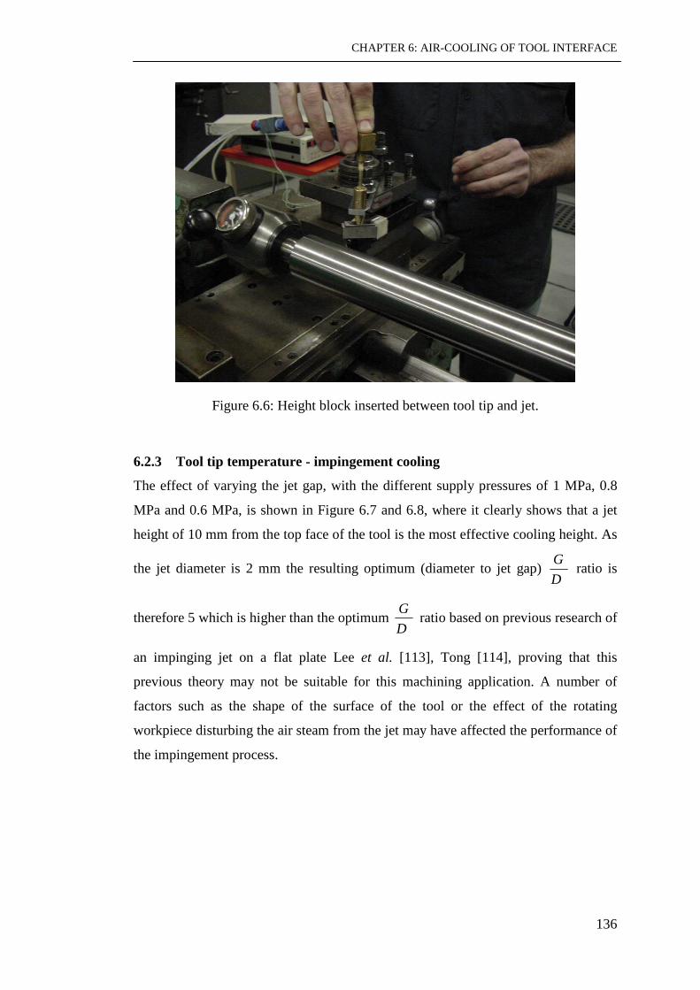
CHAPTER 6: AIR-COOLING OF TOOL INTERFACE
136
Figure 6.6: Height block inserted between tool tip and jet.
6.2.3 Tool tip temperature - impingement cooling
The effect of varying the jet gap, with the different supply pressures of 1 MPa, 0.8
MPa and 0.6 MPa, is shown in Figure 6.7 and 6.8, where it clearly shows that a jet
height of 10 mm from the top face of the tool is the most effective cooling height. As
the jet diameter is 2 mm the resulting optimum (diameter to jet gap) D
G ratio is
therefore 5 which is higher than the optimum D
G ratio based on previous research of
an impinging jet on a flat plate Lee et al. [113], Tong [114], proving that this
previous theory may not be suitable for this machining application. A number of
factors such as the shape of the surface of the tool or the effect of the rotating
workpiece disturbing the air steam from the jet may have affected the performance of
the impingement process.

CHAPTER 6: AIR-COOLING OF TOOL INTERFACE
137
75
95
115
135
155
175
195
215
5 7 9 11 13 15
Nozzle gap (mm)
To
ol t
ip t
em
pe
ratu
re (
o C
)
0.8 Mpa
1.0 Mpa
0.6 Mpa
Figure 6.7: Jet optimum height from tool tip.
The temperatures of the three thermocouples in the tool tip showed the lowest
temperature being recoded by channel 13 (Ch13), which is the position nearest to the
tool tip, which indicates heat from the tool is being removed.
8090
100110120130140150160170180
0 5 10 15
Nozzle gap (mm)
Too
l tip
tem
pera
ture
(
o C)
Ch13
Ch14
Ch15
Figure 6.8:Temperatures recorded at the tool tip for a variety of air gaps at 0.8 MPa.
The results shown in Figure 6.9 when using a 2 mm diameter exit jet at 0.8 MPa
illustrates that this method of air-cooling was able to cool the tool tip close to the
conventional wet cooling cutting temperature (100 oC) as shown in Figure 6.2.

CHAPTER 6: AIR-COOLING OF TOOL INTERFACE
138
However, although this method is capable of cooling the tool tip, it was found that
after a number of cutting tests the temperature in the workpiece became extremely
hot. This therefore indicates that additional air-cooling needs to be applied to the
workpiece to prevent dimensional inaccuracies occurring. Figure 6.7 showed that
there was no real benefit in increasing the pressure to 1 MPa from 0.8 MPa or
increasing the air gap.
0
20
40
60
80
100
120
0 5 10 15 20 25 30
Time (s)
Too
l tip
tem
per
atur
e (
o C
)
Ch13
Ch14
Ch15
Figure 6.9: Tool tip temperatures at 0.8 MPa with an air gap of 10 mm.
The result of a cutting test at 1 MPa and 10 mm air gap is shown in Figure 6.10
which interestingly shows that the temperature channel 13 (Ch13) closest to the tool
interface has increased, and the temperature further away from the tool tip has
slightly decreased. This implies that air is not penetrating as close to the tool
interface during the machining process, and the temperatures recoded at channel 14
(Ch14) and channel 15 (Ch15) were being cooled more efficiently due to the higher
air stream velocity. The greater the fluid velocity the better the heat transfer due to
the thinner boundary layer across the surface at channel 14 (Ch14) and channel 15
(Ch15), which was not occurring closer to the tool interface.

CHAPTER 6: AIR-COOLING OF TOOL INTERFACE
139
0
20
40
60
80
100
120
140
0 10 20 30
Time (s)
Too
l tip
tem
pera
ture
(
o C)
Ch13
Ch14
Ch15
Figure 6.10: Tool tip temperatures at 1 MPa with an air gap of 10 mm.
This trend is also noted when the air gap is increased to 12 mm at 1 MPa as shown in
Figure 6.11. It is well known that the flank area of the tool suffers considerable wear
during machining; it suggests that the inclusion of an additional jet directed at the
flank face will help reduce the temperature. The following tests were carried out with
a jet directed at the flank face of the tool: the results of these tests are shown on
Figure 6.12.
0
20
40
60
80
100
120
140
0 5 10 15 20 25
Time (s)
To
ol ti
p te
mpe
ratu
re (
o C
)
Ch13
Ch14
Ch15
Figure 6.11: Tool tip temperatures at 1 MPa with an air gap of 12 mm.

CHAPTER 6: AIR-COOLING OF TOOL INTERFACE
140
0
50
100
150
200
250
300
350
0 2 4 6 8 10
Time (s)
Too
l tip
tem
pera
ture
(
o C)
Dry cut
2 nozzles
Figure 6.12: Second jet directed at flank face during machining.
Unfortunately, the results were less than promising as the jet air streams interfered
with the impingement process of each of the jets. Other test configurations involved
tilting the impingement jet at an angle to the top rake face to improve clearance
between the workpiece and the jet. Figure 6.13 shows a jet after use where the side
has worn away. The position of the jet is determined by:
• tool cutting interface;
• the diameter of the workpiece;
• and the optimum air gap.
Figure 6.13: Worn jet due to being unable to obtain correct air gap without rubbing
the workpiece.

CHAPTER 6: AIR-COOLING OF TOOL INTERFACE
141
140
160
180
200
220
240
260
0 10 20 30
Time (s)
Too
l tip
tem
pera
ture
(
o C )
dry cut
2 mm air gap
4 mm air gap
8 mm air gap
10 mm air gap
Figure 6.14: Jet angled at 45 o to the rake face at a pressure of 0.8 MPa.
Figure 6.14 indicates that the cooling efficiency of the air jet angled at 45 o to the
rake face of the tool has been reduced, and also the air gap had little effect on the
performance of the cooling jet. The same is also noted for the jet angled at 60 o as
shown in Figure 6.15. This is what one would expect to happen due to the loss of the
impingement process which is gained from using a horizontal jet. Figure 6.14 and
6.15 show that there is now no beneficial effect from the surface boundary layer
breaking down and promoting a better heat transfer to the air, as both temperatures
are approximately the same indicating that the tool was only being cooled by the air
passing over the tool.
140
160
180
200
220
240
0 10 20 30
Time (s)
To
ol ti
p te
mpe
ratu
re
( o C
)
dry cut
8 mm air gap
10 mm air gap
Figure 6.15: Jet angled at 60 o to the rake face at a pressure of 0.8 MPa.

CHAPTER 6: AIR-COOLING OF TOOL INTERFACE
142
Previous tests using a one exit jet, as illustrated in Figure 6.9, have demonstrated that
there is an enhanced heat transfer to the air by using an impingement jet. It is then
logical to think that increasing the number of exit jets directed on to the top rake face
Figure 6.16 to 6.19 show multi-hole jets being used to cool the tool tip. The
effectiveness of jet-to-jet spacing for confined air jets vertically impinging on a flat
plate was investigated by Jung-Yang San et. al. [115]. As with a single exit jet it is
necessary to determine the correct air gap for the jet, how many exit holes there
should be, and at what diameter the exit hole should be for optimum cooling. Figure
6.16 shows the results from a four exit jet each of 1 mm diameter. Temperatures
recorded are compared with the single jet in Figures 6.9 and 6.10, which has the
same cross sectional area as the four exit jet.
30
40
50
60
70
80
90
100
110
120
130
0 5 10 15 20 25 30
Time (s)
Too
l tip
tem
pera
ture
(
o C)
Ch 13
Ch 14
Ch 15
Figure 6.16: Jet with 4, 1 mm nozzles.
The interesting points to note here are that the thermocouple closest to the tool tip
channel 13 (Ch13) recorded a slightly higher temperature with the four-jet than the
one jet. The temperature recorded for the thermocouples on channel 14 (Ch14) and
channel 15 (Ch15) were otherwise significantly reduced. This indicated that there
was an increased footprint being generated by this jet due to the increased number of
impingement air streams. Even though it showed that the tool interface temperature
was slightly higher, the larger footprint helped with positioning the jet at the tool tip.

CHAPTER 6: AIR-COOLING OF TOOL INTERFACE
143
It was found that if the position of the jet was out by a small amount the effectiveness
of cooling the tool tip interface was lost.
Further reduction in temperatures was achieved by increasing the number of jet exits
to eight. Figure 6.17 shows the improved cooling effect at the tool tip, with channel
14 (Ch14) recording only 45 oC this being due to the cooling air being unimpeded.
The temperatures recorded for all three thermocouples indicated a tool temperature
less than those obtained for traditional coolant as shown on Figure 6.2.
30
35
40
45
50
55
60
65
70
75
80
0 5 10 15 20 25 30
Time (s)
Too
l tip
tem
per
atu
re
( o C
)
Ch 13
Ch 14
Ch 15
Figure 6.17: Jet with 8, 1 mm nozzles.
When the number of exit holes in the jet was increased to sixteen it was interesting to
note that the thermocouple on channel 15 (Ch15) recoded temperatures below zero
degrees, and that the temperatures for the other thermocouples were approximately
10 oC higher than the four exit jet Figure 6.17.

CHAPTER 6: AIR-COOLING OF TOOL INTERFACE
144
-20
0
20
40
60
80
100
0 5 10 15 20 25 30
Time (s)
Too
l tip
tem
pera
ture
(
o C )
Ch 13
Ch 14
Ch15
Figure 6.18: Jet with 16, 1 mm nozzles.
The trend for both of these jets is the same, in that the temperature of channel 15
(Ch15) was the lowest, and that the temperatures recorded for the other two
thermocouples were quite close to each other. The reason for this improved
temperature dissipation into the air can be put down to the increased footprint that
is generated from the multi-exit holes used. Another advantage of the use of this
multi-hole jet during machining is that the air stream is penetrating nearer to the
tool tip interface. During observation of the metal cutting test it was noticed that
the chips were breaking off in small regular chips which were then blown away
from the cutting zone. Perhaps due to the cuttings being small and being swiftly
removed from the cutting zone allowed better access of the air to the tool tip.
However it must be said that any change to the cutting conditions will effect the
type of chip produced during machining, as explained in Chapter 2.

CHAPTER 6: AIR-COOLING OF TOOL INTERFACE
145
405060708090
100110120
0 10 20 30 40
Time (s)
Too
l tip
tem
pera
ture
(
o C)
Ch13
Ch14
Ch15
Figure 6.19: Three 2 mm diameter jets.
Figure 6.20: Multi-hole impinging jet nozzle.
The position of the jet relative to the tool tip is positioned to provide the maximum
coverage of the air foot print during machining as shown in Figure 6.20.

CHAPTER 6: AIR-COOLING OF TOOL INTERFACE
146
100105110115120125130135140145
0 20 40
Time (s)
Too
l tip
tem
pera
ture
(
o C)
one 2 mm dia hole
three 2 mm dia holes
three 1.1 mm diaholes
Figure 6.21: Tool temperatures for thermocouple on channel 13 (Ch13).
Figure 6.21 clearly showed that the three 2 mm diameter hole jet produced the lowest
tool tip temperature closest to the tool interface during machining. The volume of air
used during this test was 849 SLPM at the maximum test pressure (1MPa). This is
not an extremely large supply of compressed air as a typical two-stage, two-cylinder
air compressor can provide 1050 SLPM at a maximum working pressure of 1MPa
with a Motor load of 7.5 kW. This would be relatively cheap to supply as can be
calculated from equation 6.1. The cost of compressed air for one hour was calculated
to be (AU) $1 using this compressor.
Cost (AU) $ = ( )
ME
FLMLxOHxCxTx (6.1)
where ML = Motor full load in kW
OH = Number of operating hours
C = Cost per kWh
T = % of time running at this operating level
FL = % of full-load at this operating level
ME = Motor efficiency at this level

CHAPTER 6: AIR-COOLING OF TOOL INTERFACE
147
-5-4-3-2-101234
0 5 10 15
Time (s)
Too
l tem
pera
ture
(
o C)
Ch13
Figure 6.22: Tool temperature before cutting using three – 2 mm diameter jet.
Figure 6.23: Frost on impingement jet nozzle before machining.
The graph in Figure 6.22 was obtained before any machining had taken place and
clearly indicates the effectiveness of the impingement cooling of the tool tip.
Figure 6.23 shows a build up of frost on the jet nozzle. In practice, however, the
efficiency of the cooling of the tool tip is reduced due to the cutting action during
machining.
6.3 Vortex Tube Cooling During Metal Cutting
6.3.1 Tool tip temperature during vortex tube air-cooling
Unlike the impingement cooling process there is no difference to the cooling effect
by adjusting the distance that the cold tube nozzle is from the tool tip. The nozzle
does not need to be perpendicular to the rake face - unlike the impingement jet

CHAPTER 6: AIR-COOLING OF TOOL INTERFACE
148
nozzle - to be effective. Although, the closer the cold tube nozzle jet is to the tool
face, the less time there is for the surrounding ambient temperature to begin to affect
the cold stream of air. Figure 6.24 shows the vortex tube directing the cold airflow
onto the tool face as close as the machining restraints will allow. A series of tests
involving the various cutting parameters and positioning of the vortex tube were
performed to determine their effects on the cooling performance. The parameters
were changed systematically as outlined in Appendix D while the machining
conditions were kept constant throughout the tests.
Figure 6.24: Vortex tube being positioned with respect to machining restraints.
The temperatures shown in Figure 6.25 were recorded at the tool tip during
adjustment of the conical valve on the vortex tube at an inlet pressure of 0.8 MPa.
Setting the valve normally takes about thirty seconds to achieve the optimum cold
exit air. Having obtained the minimum air temperature, machining can commence.
During this time the cold air had already started to cool the tool tip down, with two
of the thermocouples recording temperatures of approximately –5 oC.
Reducing the inlet air pressure to 0.4 MPa the cold exit air temperature was
approximately -15 oC, which correspondingly reduces the tool tip temperature down

CHAPTER 6: AIR-COOLING OF TOOL INTERFACE
149
to approximately -3 oC in double the time achieve by 0.8 MPa. The time factor is
important in cooling the tool tip, as the rise in temperature during machining is
extremely fast. It is therefore imperative to be able to dissipate the generated heat in
the tool tip as quickly as possible.
The vortex tube used a 3 mm diameter orifice plate at a pressure of 0.8 MPa
Figure 6.25: Tool tip temperatures before machining.
When the vortex exit air has reached approximately -30 oC, machining is
commenced. As indicated by the rise in the tool tip temperatures, the tip rises to a
steady state temperature of 60 oC channel 13 (Ch13) as shown in Figure 6.26. The
temperature drop at the end indicates the point when the feed is stopped with no
more chips being generated. Allowing the cooling air to flow unimpeded across the
tool tip gives a better heat dissipation from the tool reducing the temperature in the
tool rapidly.

CHAPTER 6: AIR-COOLING OF TOOL INTERFACE
150
Figure 6.26: The graph shows the tool tip temperatures during machining, and after
the tool feed has stoped cutting.
Figure 6.27 illustrates that a steady state temperature is reached in the tool tip in
approximately 10 seconds during machining when being cooled by the vortex tube.
However, it is noticeable that there is still a large temperature difference between the
temperature closest to the tool interface channel 13 (Ch13), and that of the
temperatures further from the tool interface channel 14 (Ch14) and channel 15
(Ch15). The inability of the air to penetrate close to the tool interface is undoubtedly
due to the cold exit jet needing to be positioned away from the cutting zone due to
the operating requirements. This is providing the cooled air closer to the tool
interface would improve the accessibility of the air to the cutting zone, and would
therefore improve further the heat dissipation at the tool tip. This challenge of
improving the cold air delivery to the tool tip can be achieved by combining the cold
air generated by the vortex tube with an air jet being incorporated as part of a chip
breaker as shown in Figure 6.30. Even without this improved jet the reduction in
temperature between dry machining and the air cooled temperature is extremely
effective, and proves the case for air-cooling as shown in Figure 6.28. Appendix E
gives an example of the data recorded during the tool cutting tests.

CHAPTER 6: AIR-COOLING OF TOOL INTERFACE
151
25
35
45
55
65
75
85
95
105
115
0 10 20 30 40
Time (s)
To
ol t
ip te
mp
erat
ure
o C
Ch13
Ch14
Ch15
The vortex tube used a 4.5 mm diameter orifice plate at a pressure of 0.8 MPa.
Figure 6.27: Temperatures recoded at the tool tip during machining.
0
50
100
150
200
250
0 5 10 15 20 25
Time (s)
Too
l tip
tem
pera
ture
(
o C)
vortex air
dry cut
Figure 6.28: Temperatures recoded at the tool tip for dry and air-cooling.
Figure 6.29 illustrates the relationship between the hot air and the cold air generation
of the vortex tube. From Chapter 4 experimental analysis of vortex tube design, it
shows that the length of the hot tube has an important effect on the energy separation
in the vortex tube, due to the air inner flow transfer of energy to the outer airflow.
However, the vortex tube used in that tool test did not achieve the optimum

CHAPTER 6: AIR-COOLING OF TOOL INTERFACE
152
temperature difference between the hot and cold air exit. The optimum hot tube
length was not used due to it being unmanageable and impractical to use on the lathe.
The compromise of using a shorter vortex tube still proved to be effective as it was
capable of producing cold air at -30 oC as shown on Figure 6.26.
-20
-15
-10
-5
0
5
10
15
20
25
0 10 20 30 40 50 60
Time (s)
Exi
t tem
erat
ure
(
o C)
Hot outlet
Cold outlet
Figure 6.29: Air exit temperatures of hot and cold exit of the vortex tube.
Figure 6.30 showed that the vortex tube used in these tests was able to generate very
cold air at the exit of the cold jet. A temperature of -55 oC was obtained by using an
inlet pressure 1MPa to the vortex generator.
-60
-50
-40
-30
-20
-10
0
10
0 50 100 150
Time (s)
No
zzle
exi
t tem
per
atu
re (o
C)
Figure 6.30: Vortex tube minimum air exit temperature.

CHAPTER 6: AIR-COOLING OF TOOL INTERFACE
153
6.3.2 Chip breaker air jet cooling
The effectiveness of air-cooling can be further improved by directing the cooled air
more precisely at the tool interface during machining. To achieve this difficult task it
is thought that combining an air jet nozzle, as part of a tool chip breaker, with an
additional jet directing the air towards the flank face could be a possible solution to
this challenge. Figure 6.31 shows the internal air channels to the tool interface jet,
and Figure 6.32 & 6.33 shows the prototype lathe cutting tool directing air along the
tool top rake face and flank face during machining. The cold air is supplied from the
integral tool and vortex tube arrangement as shown in Figure 6.34 & 6.35.
Figure 6.31: Lathe cutting tool and combined air jets and chip breaker drawing.
Figure 6.32: Top rake face air and flank face air jets.
The arrows in Figure 6.32 show the two air jets directing the cold air towards the
cutting zone. In addition to the cooling effect of the air is the advantage of blowing
the cuttings away from the cutting zone as can be seen from Figure 6.33. As this was

CHAPTER 6: AIR-COOLING OF TOOL INTERFACE
154
a prototype tool an additional front metal guard was employed to protect the
thermocouples during machining. Close examination of the cutting process shows
that the air stream is being directed underneath the chip as can be seen in Figure 6.33
promoting a better heat dissipation from the tool-cutting zone.
At a feed rate of 0.23 mm/rev and 1 mm depth of cut.
(Air being directed along top rake face and underneath the chip)
Figure 6.33: Orthogonal machining using a chip breaker incorporating air jets.
Figure 6.34: Vortex tube integral with tool body.

CHAPTER 6: AIR-COOLING OF TOOL INTERFACE
155
Figure 6.35: Continuous dark blue chip shown being produced during machining
with the integral vortex tube and tool.
The temperatures recorded at the jets during machining proved to be disappointing
for this prototype tool as the air never got lower than 2 oC, with the resulting tool tip
temperatures during cutting being recorded hotter. Obviously, the combination of the
vortex tube, lathe tool and jets was not working in this configuration. From theory
and previous testing of the vortex tube the air temperature leaving the rake jet never
obtained its normal cold temperature. To determine what the temperature should be
in the tool body, thermocouples are inserted along an 8 mm diameter tube as shown
in Figure 6.36 to record the temperatures along the tube. Being the same length and
diameter that was used in the prototype tool this should measure what the
temperatures should be inside the tool and as it exits the jet. The results from this test
showed that the air stream leaving the jet should be approximately –16 oC. This
temperature implies that the vortex cooling effect is breaking down in the prototype
tool. Examination of the prototype tool shows that the jet exit area was not large
enough, causing a back-pressure in the vortex generator. To improve the
performance of the prototype tool the volume flow rate needs to be increased to
remove the backpressure inside the cold vortex tube which is stopping the vortex
cooling effect. This was achieved by increasing the size of the rake face air jet.

CHAPTER 6: AIR-COOLING OF TOOL INTERFACE
156
However, the top rake jet exit area needs to be within the physical restraints of the
tool and the size should avoids chips being tangled with the jet.
-24
-23
-22
-21
-20
-19
-18
-17
-16
-15
0 2 4 6 8 10
Thermocouple position along cold tube
Tem
pert
ure
( o C)
Figure 6.36: Temperatures distribution along an 8 mm diameter vortex cold exit tube.
A second prototype tool implements the increased size of top rake air jet and flank
face air jet as shown in Figure 6.37. The combined cross-sectional area of the air jets
must not be less than the area of the exit diameter from the vortex tube to ensure
maximum air-cooling. Increasing the size of flank face jet was the most convenient
way to achieve the increased jet exit area due to the physical restraints of the tool.
This increased jet exit area produced the desired result, in that the recorded
temperature of the air at the exits has been reduced to -6 0C as shown in Figure 6.39.
Although when this temperature is compared with the temperatures recorded in
Figure 6.36, it proves that there are still some improvements to be made to the
combined vortex tube and tool.

CHAPTER 6: AIR-COOLING OF TOOL INTERFACE
157
Figure 6.37: Prototype tool showing increased flank face jet.
The practicability of using this tool is somewhat limited in this form due to its
inability to be able to machined up to a shoulder and limited depth of cut. However,
the tool did prove the benefits of providing directed cold air at the tool interface
during machining.
Figure 6.38: Cold air stream delivered at flank face and top rake face.
Another approach to ensure that there is no backpressure into the vortex tube is by
allowing the cold air stream from the vortex to be split. The larger volume of cold air

CHAPTER 6: AIR-COOLING OF TOOL INTERFACE
158
will be directed from the vortex jet onto the tool tip as shown in Figure 6.38, with a
smaller amount of cold air being delivered to the flank face of the tool.
Figure 6.39: Temperature produced by the second prototype tool before machining
takes place.
Figure 6.40: Frost on the outside of the cold tube.
The temperature that was recorded for the tool tip using the chip breaker and flank jet
is similar in value to what was achieved by the previous methods of air-cooling as
shown by Figures 6.22 and 6.25. However, the advantage of the chip breaker and
flank jet is that the air is focused directly on to the areas of the tool that generate the
most heat and where maximum wear takes place.

CHAPTER 6: AIR-COOLING OF TOOL INTERFACE
159
6.4 Tool Life
6.4.1 Effect of air-cooling on tool life
In Chapter 2 it is clearly shown that all the wear mechanisms increased at elevated
temperatures, reducing the tool life. The previous sections illustrated that applying
cold air to the tool tip is capable of reducing the temperature at the tool tip enabling
the tool tip to have a longer tool life. The effectiveness of the air-cooled system can
be shown when a comparison is made between the wear for a dry cut and an air-
cooled cut for one minute and seven minutes of machining. Figure 6.41 to 6.44
shows the flank wear as seen under a microscope with a 63 optical magnification
setting.
At a cutting speed of 190 m/min and feed rate of 0.23 mm/rev with a 2 mm depth of cut.
Figure 6.41: Picture showing flank wear of a dry cut after 1 minute of machining.
At a cutting speed of 190 m/min and feed rate of 0.23 mm/rev with a 2 mm depth of cut.
Figure 6.42: Picture showing flank wear of an air-cooled cut after 1 minute of
machining.

CHAPTER 6: AIR-COOLING OF TOOL INTERFACE
160
At a cutting speed of 190 m/min and feed rate of 0.23 mm/rev with a 2 mm depth of cut.
Figure 6.43: Picture showing flank wear of a dry cut after 7 minutes of machining.
The development of the flank wear was shown to take longer to develop when the
cooled air was applied to the cutting zone as shown in Figure 6.44.
At a cutting speed of 190 m/min and feed rate of 0.23 mm/rev with a 2 mm depth of cut.
Figure 6.44: Picture showing flank wear for an air-cooled cut after 7 minutes of
machining.
After seven minutes of dry machining the top rake face is starting to develop crater
wear at 0.5 mm from the flank face as shown in Figure 6.45. Further dry machining
will accelerate this rate of wear. At this stage the tool radius shows no sign of wear
and the top flank edge has no observable notches.

CHAPTER 6: AIR-COOLING OF TOOL INTERFACE
161
At a cutting speed of 190 m/min and feed rate of 0.23 mm/rev with a 2 mm depth of cut.
Figure 6.45: Picture showing top rake face wear for a dry cut after 7 minutes of
machining.
At a cutting speed of 190 m/min and feed rate of 0.23 mm/rev with a 2 mm depth of cut.
Figure 6.46: Picture showing top rake face wear for air-cooled cut after 7 minutes of
machining.
With the air-cooled tool tip there are no visible signs of tool wear on the top rake
face Figure 6.46, and the flank wear shown in Figure 6.41 and 6.42 is substantially
reduced. Observation of the chips produced during dry and air-cooling indicated that
much of the heat was being dissipated from the cutting zone. Figure 6.47 shows the
chips produced during the dry and air-cooled tool tip test. From the colour of the
chips a guide to the relative temperature can be made. Referring to Figure 5.2, dark
blue (dry) indicates the chip temperature was approximately 750 oC, and gold
indicates the chip temperature was approximately 600 oC.

CHAPTER 6: AIR-COOLING OF TOOL INTERFACE
162
At 0.23 m/rev. feed rate, and cutting speed of 190 m/min.
Figure 6.47: Chips produced by a 2 mm depth of cut.
6.4.2 Discussion
Both the impingement and vortex tube experimental air-cooling systems have proved
capable of dissipating the heat from the tool tip, proving that air-cooling is an
effective method of cooling tools and increases the tool life. Whenever dry
machining is considered to be the preferred method of metal cutting, it should be
good practice to incorporate air-cooling. Also, air-cooling should be considered as an
alternative to liquid cooling, as it was shown in this research that by reducing the
temperature of the air, the tool is cooled to a point compatible with traditional
coolant. Using an air-cooling system is found to be cost effective as there are no
disposal costs associated with cooling, and is an environmentally friendly process.
For practical operating reasons the vortex tube is the preferred option as it is more
convenient for the machine operator to use as exact positioning of the cold air exit is
not necessary. In addition the vortex tube is capable of cooling the air to –30 oC by a
relatively low pressure supply of 0.8 MPa, which most workshops have readily
available, making it convenient to use.
The most convenient method of determining tool life in this research is by using the
tool tip temperature, as it has been shown that there is a relationship between the tool
life and the wear mechanisms, which is shown to increase at elevated cutting
temperatures. It was observed that when machining at the normal cutting speed for
carbide tool tips it is not usual for the cutting tool temperatures to be above 800 oC.
The result of this is the main wear mechanism is diffusion, and the temperature
controls the rate of the wear process. Therefore, knowing the appropriate tool
temperature, it should be possible to predict tool life when the tool life is defined in
Air-cooled Dry cutting

CHAPTER 6: AIR-COOLING OF TOOL INTERFACE
163
terms of the flank ware. The relationship between tool life L, and the tool flank
temperature, Tf can be obtained from equation (3.12) using the constants that are
correct for their cutting conditions. However, equation (6.2) in the form of (3.12) has
proved useful in determining the tool life, when using the temperature recorded from
the imbedded thermocouple. The constants used reflect that the temperature that is
measured in the tool tip is not as high as would be obtained from the tool flank face
Tf.
58.0974.210 thTL = (6.2)
The tool performance in section 6.4 examined tool tips which were tested over the
same length of time and to ensure that the tool tips were being compared having
completed the same amount of cutting. Even with measuring the tool tip temperature
during the test there is still considerable time involved in completing all the tests to
show the tool wear.
It may sound an easy challenge to measure or calculate the tool interface
temperature, but as previously shown this task is fraught with difficulties. For
example, there are large differences in temperature between the tool flank face and
the position of the thermocouple that are measuring the tool temperature in the
cutting zone. This makes it necessary to calculate the flank face temperature by using
equation (3.15), which can be used to determine the tool life for the tool. If it is not
possible to use the tool temperature to calculate the tool life then the only option is to
carry out numerous tool cutting tests. However, to reduce the number of tool life
tests it seems only logical that the factorial regression analysis method be used to
determine the tool life constants for equation (3.2). Even with this method the
number of required tool life tests are substantially making tool life tests time
consuming and expensive, although the data that is obtained is precious in
determining the performance of any cutting tool.
Previous researchers such as Liu et al. [116], [42] proved that compressed air did not
achieve as good heat dissipation as oil water emulsion or water vapour during metal
cutting as was shown in Figure 2.20. However, the results obtained from using

CHAPTER 6: AIR-COOLING OF TOOL INTERFACE
164
compressed air combined with the vortex tube have shown that this method of
cooling the cutting zone is effective and compares exceedingly well with traditional
methods. The effectiveness of air-cooling may be further improved by directing cold
air through an air jet incorporated in the chip breaker on top of the tool.

CHAPTER 7: CONCLUSIONS
165
CHAPTER 7
CONCLUSIONS
7.1 Introduction
Removing the liquid coolant from the machining process presents numerous
challenges relating to machining, the primary challenges being heat dissipation from
tool and workpiece, tool life, and chip removal. Certain systems and strategies can of
course address these challenges. Heat removal by air requires a different approach to
reduce the temperature of the tool tip compared to heat removal by liquid coolant.
Special tooling using jet ducts, high-performance coated tool tips and chip
evacuation systems may also be required in cooling the tool tip without the use of
liquid coolant. When air-cooling is used it is necessary to show that the tool life is
unchanged from wet machining and that the work piece quality is as good as, or
better than, wet machining.
7.2 Significance And Outcomes
The significance of reducing the environmental burden produced by industry is now
a prime objective, due to governmental registration and international regulations. For
metal cutting the main source of environmental pollution is associated with
traditional use of liquid coolants. This thesis has proved that air cooling can
contribute to reducing or eliminating the reliance on liquid coolant used in metal
cutting. Over the last few years some manufacturing industries have adopted dry
machining for ductile materials which are relatively easy to machine. For harder
materials coolant is found to be necessary to extend the tool life. The addition of air
cooling for the machining of these materials is shown to have the same effect of
extending the tool life. Therefore, for the majority of materials being machined in
industry the use of air cooling is shown to be effective without adding to the cost of
producing the product. In addition to the cost saving, the machine operators’ health
and working conditions will be improved as no liquid coolant is being used.

CHAPTER 7: CONCLUSIONS
166
It has been shown that both impingement cooling and vortex tube cooling are capable
of reducing the tool tip temperature during machining. The vortex tube air-cooling
method has proved to be the most practical to use; it has also been found to be more
robust and much easier to use. The vortex tube jet - unlike the impingement jet - had
no reliance on jet operation position to produce the cooling effect on the tool tip. The
vortex tube can be integral to the cutting tool because it does not have to rely on the
position of the jet for the cooling. A combined vortex tube and lathe tool now has the
advantage of being able to direct cold air along the rake face towards the tool cutting
zone.
This thesis shows the beneficial effects of using air-cooling in metal cutting, and will
help persuade the manufacturing industry to adopt this environmentally friendly air-
cooling system. Worldwide saving in the amount of liquid coolant used would be
enormous due to the massive amount of machining that is carried out, since metal
cutting is still the primary manufacturing process used. Productivity and efficiency
gains are the main advantages of having an effective air-cooling system as part of the
metal cutting process: less money will be spent on tools and coolant. The goal is to
keep the cutting edge “cutting”, as productivity depends on reducing insert changing
or indexing, i.e. cycle times, to produce a higher metal removal rate and consistent
quality. These issues are overwhelmingly important to manufacturers, and air-
cooling will help improve productivity by extending tool life when dry machining.
7.3 Recommendations And Possible Further Developments
Obtaining the temperature profiles of the tool tip allowed tool life expectancy to be
determined for each of the cutting conditions. It is very important to be able to
conveniently measure the tool tip temperature as this allows for an easy, reliable and
quick method of determining the tool life. Recent developments in infrared
measurement now allow you to measure the tool tip even more accurately than
before, allowing the tool temperature to be used to give good estimates of tool life.
Future developments in this technology may be the inclusion of a very small quantity
of oil to reduce the friction of the chip as it slides over the top rake face. Improving
the chip removal from the cutting zone improves the air-cooling system. Materials

CHAPTER 7: CONCLUSIONS
167
that create fine dust or fine cuttings need to be safely removed from the cutting area.
Other machining operations such as drilling require further investigation to establish
how best to provide cold air to the cutting edge of the drill.
The vortex tube method has been shown to be very effective for spot cooling, and the
device itself is very simple, making it ideal for use in the workshop. Endeavour to
reduce the temperature further at the cold exit jet is to take the cold exit air and pass
it through a second stage vortex tube. This is only possible if there is sufficient
pressure when the cold air leaves the cold exit. Another development which needs to
be examined is how some other inert gas (eg. nitrogen) works with the vortex tube,
as this may further improve the performance of cooling the tool tip. Carbon dioxide
was tried in the mid 1950’s, but was soon given up due to the cost of plant, and at
that time environmental considerations were sadly of no great concern to the
manufacturing industry.
7.4 Conclusion
Good classical thinking in metal cutting states that the best ratio of high productivity
to low tool cost is obtained by selecting the maximum depth of cut and feed for the
given situation. This thinking is correct as long as the tool tip can maintain an
effective tool life, and produce the required surface finish. Using an efficient vortex
tube to cool the tool during machining satisfies these conditions. This combination of
air-cooling and dry machining gives an effective environmental tool cooling process.
Twenty years ago the management and disposal of cutting fluids accounted for less
than 3 percent of the production costs; today the cost has risen to 16 percent. Such
costs explain why manufacturers are desperately looking for alternative methods to
liquid coolant for cooling tool tip. This research has proven then that air-cooling
using a vortex tube can certainly be considered as one of those methods.

REFERENCES
168
REFERENCES
[1] M. E. Merchant, "Delphi-Type Forecast of the Future of Production
Engineering," C.I.R.P. Annals, vol. 20, p. 213, 1971.
[2] E. J. A. Armarego and R. H. Brown, The Machining of Metals. New Jersey:
Prentice-Hall, Inc, 1969.
[3] I. Finnie, "Review of the Metal Cutting Analyses of the Past Hundred Years,"
Mechanical Engineering, vol. 78, p. 715, 1956.
[4] W. Rosenhain and A. C. Sturney, "Report on Flow and Rupture of Metals
During Cutting," Proc. I. Mech. E., vol. 1, p. 141, 1925.
[5] H. Ernst, "Physics of Metals: Machining of Metals," American Soc. for
Metals, 1938.
[6] G. C. I. Lin and P. l. B. Oxley, "Mechanics of Oblique Machining: Predicting
Chip Geometry and Cutting Forces from Work Material properties and
Cutting Conditions," Proc. I. Mech. E., vol. 186, p. 813, 1972.
[7] M. P. Groover, Fundamentals of Modern Manufacturing: John Wiley and
Sons. Inc, 2006.
[8] M. D. Centre, Machine Data Handbook, Third ed. vol. one. Cincinnati Ohio:
Metcut Research Assoc. Inc, 1980.
[9] http://www.feret.com.au/c/Seco-Tools- Australia/Milling-turning-anddrilling-
inserts-n689736, Uploaded on 26th January 2006.
[10] G. Boothroyd, "Temperature in Orthogonal Metal Cutting," Proc. I. Mech. E.,
vol. 177, p. 789, 1963.
[11] H. Narita, H. Kawamura, T. Norihisa, L. Y. Chen, and H. Fujimoto,
"Manufacturing Process Evaluation using Environmental Burden Analyzer

REFERENCES
169
for Machine Tool Operation," in 18th International Conference on
Production Research, Salerno, Italy, 2005.
[12] D. Dudzinski, A. Devillez, A. Moufki, D. Larrouquere, V. Zerrouki, and J.
Vigneau, "A review of developments towards dry and high speed machining
of Inconel 718 alloy," International Journal of Machine Tools and
Manufacture, vol. 44, pp. 439-456, 2004/3 2004.
[13] K. H. Causton, "An investigation into the suitability of dry machining
automotive cylinder blocks for high volume production," in Engineering
Bradford: University of Brdford, 2002.
[14] N. A. Abukhshim, P. T. Mativenga, and M. A. Sheikh, "Investigation of heat
partition in high speed turning of high strength alloy steel," International
Journal of Machine Tools and Manufacture, vol. In Press, Corrected Proof,
2005.
[15] B. T. Chao, H. L. Li, and K. J. Trigger, "The Influence of Tool Geometry on
Interface Temperatures," M.E. Tech. Rep., 1957.
[16] P. L. B. Oxley, "Mechanics of Metal Cutting for a Material of Various Flow
Stress," Trans. ASME, vol. 85, p. p. 339, 1963.
[17] H. Ernst and M. E. Merchant, "Chip Formation, Friction and High Quality
Machined Surfaces," American Soc. for Metals, p. 229, 1941.
[18] D. G. Christopherson, P. l. B. Oxley, and W. B. Palmer, "Orthogonal Cutting
of a Work-hardened Material," Engineering, vol. 186, p. 623, 1959.
[19] Y. Altintas, Manufacturing Automation: Cambridge University Press, 2000.
[20] J. H. Weiner, "Shear Plane Temperature Distribution in Orthogonal Cutting,"
Trans. ASME, vol. 77, p. p. 1331, 1956.

REFERENCES
170
[21] M. G. Steven and P. L. B. Oxley, "An Experimental Investigation of the
Influence of Strain-rate and Temperature on the Flow Stress Properties of
Low Carbon Steel Using a Machining Test," Proc. I. Mech. E., vol. 185, p.
pp. 741, 1971.
[22] N. Cook, "Tool Wear and Tool Life," ASME Transactions, vol. 95, pp. pp.
931-938, 1973.
[23] H. Saglam, F. Unsacar, and S. Yaldiz, "Investigation of the effect of rake
angle and approaching angle on main cutting force and tool tip temperature,"
International Journal of Machine Tools and Manufacture, vol. 46, pp. 132-
141, 2006/2 2006.
[24] H. A. Kishawy, M. Dumitrescu, E.-G. Ng, and M. A. Elbestawi, "Effect of
coolant strategy on tool performance, chip morphology and surface quality
during high-speed machining of A356 aluminum alloy," International
Journal of Machine Tools and Manufacture, vol. 45, pp. 219-227, 2005/2
2005.
[25] M. E. Merchant, "The action of cutting fluids in machinery," Iron and Steel
Engineering, vol. 27, pp. 101 -108, 1950.
[26] S. Kalpakjian and S. R. Schmid, Manufacturing Engineering and
Technology, 5th ed.: Pearson Pretice Hall, 2005.
[27] M. C. Shaw, N. H. Cook, and P. A. Smith, "The Mechanics of Three-
dimentional Cutting Operations," Transactions of ASME, pp. 1055-1064,
1962.
[28] F. Eugene, "Ann," CIRP, vol. 52(1), pp. 13-17, 1952.
[29] M. C. Shaw, J. D. Pigott, and L. P. Richardson, "Effect of Cutting Fluid upon
Chip-Tool Interface Temperature," Trans. Of ASME, vol. 71, pp. 45-56, 1951.

REFERENCES
171
[30] C. F. Shaw and M. Hattori, "Cost and Process Information Modelling for Dry
Machining," CiteSeer.ist, pp. 1-8, 2004.
[31] P. Zelinski, "Where Dry Milling Makes Sense." vol. 2005: MMS Online,
2005.
[32] F. Georgia, "Near Dry Machining Means Improvements For Roof Rack
Manufacturing." vol. 2005: MMS Online, 2005.
[33] A. E. Diniz and A. Jose de Oliveira, "Optimizing the use of dry cutting in
rough turning steel operations," International Journal of Machine Tools and
Manufacture, vol. 44, pp. 1061-1067, 2004/8 2004.
[34] A. E. Diniz and R. Micaroni, "Cutting conditions for finish turning process
aiming: the use of dry cutting," International Journal of Machine Tools and
Manufacture, vol. 42, pp. 899-904, 2002/6 2002.
[35] A. E. Diniz and R. Micaroni, "Influence of the direction and flow rate of the
cutting fluid on tool life in turning process of AISI 1045 steel," International
Journal of Machine Tools and Manufacture, vol. In Press, Corrected Proof.
[36] A. S. Varadarajan, P. K. Philip, and B. Ramamoorthy, "Investigations on hard
turning with minimal cutting fluid application (HTMF) and its comparison
with dry and wet turning," International Journal of Machine Tools and
Manufacture, vol. 42, pp. 193-200, 2002/1 2002.
[37] M. Rahman, A. Senthil Kumar, and M. U. Salam, "Experimental evaluation
on the effect of minimal quantities of lubricant in milling," International
Journal of Machine Tools and Manufacture, vol. 42, pp. 539-547, 2002/4
2002.
[38] R. J. Piggot and A. T. Coldwell, "H-jet system for increasing tool life," SAE
Quarterly Transanction, vol. 6, pp. 547-564, 1952.

REFERENCES
172
[39] P. Dahlman and M. Escursell, "High-pressure jet-assisted cooling: a new
possibility for near net shape turning of decarburized steel," International
Journal of Machine Tools and Manufacture, vol. 44, pp. 109-115, 2004/1
2004.
[40] V. V. Podgorkov, "Method of Cutting in Application," in Patent of USSR
#1549721 MCI B23Q Russia, 1992.
[41] V. A. Godlevski, "Water Steam Lubrication During Machining," Tribologia,
vol. 162, pp. 890-901, 1998.
[42] J. Liu, R. Han, and Y. Sun, "Research on experiments and action mechanism
with water vapor as coolant and lubricant in Green cutting," International
Journal of Machine Tools and Manufacture, vol. 45, pp. 687-694, 2005/5
2005.
[43] S. Y. Hong and Y. Ding, "Cooling approaches and cutting temperatures in
cryogenic machining of Ti-6Al-4V," International Journal of Machine Tools
and Manufacture, vol. 41, pp. 1417-1437, 2001/8 2001.
[44] S. Y. Hong, Y. Ding, and W.-c. Jeong, "Friction and cutting forces in
cryogenic machining of Ti-6Al-4V," International Journal of Machine Tools
and Manufacture, vol. 41, pp. 2271-2285, 2001/12 2001.
[45] F. W. Taylor, "On the art of cutting metal," Trans. ASME, vol. 28, p. 31,
1907.
[46] J. Talylor, "The tool wear-time relationship in metal cutting," Int. J. Mach.
Tool Des. and Res., vol. 2, p. 119, 1962.
[47] R. Woxen, Tool-life and Balance of Heat in lathe work vol. 142. Stockholm:
Handlingar, 1937.

REFERENCES
173
[48] B. N. Colding, A wear relationship for turning, milling and grinding.
Stockholm: Lund Press, 1959.
[49] D. A. Axinte, W. Belluco, and L. De Chiffre, "Reliable tool life
measurements in turning -- an application to cutting fluid efficiency
evaluation," International Journal of Machine Tools and Manufacture, vol.
41, pp. 1003-1014, 2001/5 2001.
[50] A. L. B. Dos Santos, M. A. V. Duarte, A. M. Abrao, and A. R. Machado, "An
optimisation procedure to determine the coefficients of the extended Taylor's
equation in machining," International Journal of Machine Tools and
Manufacture, vol. 39, pp. 17-31, 1999/1 1999.
[51] K. J. Trigger and B. T. Chao, "The mechanisim of creater wear of cemented
carbide tools," Trans. ASME, vol. 78, p. 1113, 1956.
[52] J. Sata, "Crater wear of carbide cutting tools," Nihon Kikai Gakkai
Ronbunshu, vol. 25, p. 988, 1959.
[53] E. G. Lowen and M. C. Shaw, "On the analysis of cutting tool temperatures,"
Trans. ASME, vol. 76, p. 217, 1954.
[54] H. Takayama and R. Murata, "Basic investigation of tool wear," Trans.
ASME, J. Eng. Ind., vol. 85, p. 33, 1963.
[55] P. l. B. Oxley, W. F. Hastings, and M. G. Stevenson, "Predicting cutting
forces, tool life,etc. using work material flow stress properties obtained from
high speed compression tests," in Proc. Int. on Prod. Eng., Tokyo, 1974, p.
528.
[56] G. Boothroyd, J. M. Eagle, and A. W. J. Chisholm, "Effect of tool flank wear
on the temperatures generated during metal cutting," in Proc. 8th Int.
M.T.D.R. Conf., 1967, p. 667.

REFERENCES
174
[57] W. F. Hastings and P. l. B. Oxley, "Predicting tool life from fundamental
work material properties and cutting conditions," C.I.R.P. Annals, vol. 25/1,
p. 33, 1976.
[58] B. T. Chao and K. J. Trigger, "Cutting temperatures and metal cutting
phenomena," Trans. ASME, vol. 73, p. 777, 1951.
[59] R. N. Richardson, W. F. Hastings, and P. l. B. Oxley, "Predicting tool-life
and built-up edge occurrence when machining plain carbon steel with high
speed cutting tools," I. E. Aust., vol. ME3, p. 50, 1978.
[60] W. F. Hastings, P. Mathew, P. l. B. Oxley, and J. Talylor, "Estimated cutting
temperatures - their use as a predictor of tool performance when machining
plain carbon steel," in 20th Int. M.T.D. R. conference, 1979, p. 313.
[61] A. A. Zakaria and J. I. Gomayel, "On the reliability of the cutting temperature
for monitoring tool wear," Int. J. Mach. Tool Des. and Res., vol. 15, p. 195,
1975.
[62] T. N. Loladge, "Adhesion and diffussion wear in metal cutting," Inst. Engrs.
India, vol. 43, p. 108, 1962.
[63] H. Suzuki and T. Yamamoto, "Cratering wear of cemented carbides in
relation to carbon content in tools and machined steel," Trans J.I.M., vol. 10,
1969.
[64] N. Narutaki and Y. Yamane, "Wear mechanism of carbide tool based on the
reaction between tool and work material," Bull. Japan Soc. Prec. Eng., vol.
10, pp. 95 - 133, 1976.
[65] L. Walter, "Carbon dioxide as cutting tool coolant repays research with
imposing savings," Canadian Machining and Metalworking, vol. 76, p. 94,
1965.

REFERENCES
175
[66] W. S. Hollis, "The application and effect of controlled atmosheres in the
machining of metals," Int. J. Mach. Tool Des. and Res., vol. 1, p. 59, 1961.
[67] G. Pahlitzsch, "Gases are good cutting coolants," American Machinist, vol.
97, p. 196, 1953.
[68] M. Angioletti, R. M. Di Tommaso, E. Nino, and G. Ruocco, "Simultaneous
visualization of flow field and evaluation of local heat transfer by transitional
impinging jets," International Journal of Heat and Mass Transfer, vol. 46,
pp. 1703-1713, 2003/5 2003.
[69] D. H. Lee, Y. S. Chung, and M. G. Kim, "Technical NoteTurbulent heat
transfer from a convex hemispherical surface to a round impinging jet,"
International Journal of Heat and Mass Transfer, vol. 42, pp. 1147-1156,
1999/3/1 1999.
[70] M. Angioletti, E. Nino, and G. Ruocco, "CFD turbulent modelling of jet
impingement and its validation by particle image velocimetry and mass
transfer measurements," International Journal of Thermal Sciences, vol. 44,
pp. 349-356, 2005/4 2005.
[71] D. Hee Lee, S. Youl Won, Y. Taek Kim, and Y. Suk Chung, "Turbulent heat
transfer from a flat surface to a swirling round impinging jet," International
Journal of Heat and Mass Transfer, vol. 45, pp. 223-227, 2002/1 2002.
[72] F. P. Incropera and D. P. De Witt, Fundamentals of Heat and Mass Transfer:
John Wiley, 1981.
[73] J.-Y. San, C.-H. Huang, and M.-H. Shu, "Impingement cooling of a confined
circular air jet," International Journal of Heat and Mass Transfer, vol. 40, pp.
1355-1364, 1997/4 1997.

REFERENCES
176
[74] G. Ranque, "Experiences sur la detente giratore avec productions simulanees
d'un echappement d'air chaud et d'um echappement d'air froid," Journal de
Physique et de la Radium, vol. 4, pp. 1125-1155, 1933.
[75] R. Hilsch, "The use of the expansion of gases in a centrifugal field as a
cooling process," The review of Sicentific Instrumets, vol. 18(2), p. 108ff,
1947.
[76] R. G. Deissler and M. Perlmutter, "Analysis of the flow and energy
separation in a turbulent vortex," International Journal of Heat and Mass
Transfer, vol. 1, pp. 173-191, 1960/8 1960.
[77] M. Kurosaka, "Acoustic streaming in swirling flow," Journal of Fluid
Mechanics, p. 139ff, 1982.
[78] A. I. Gulyaev, "Vortex tube and the vortex effect," Soviet Physics: Technical
Physics, vol. 10(10), p. 1441ff, 1966.
[79] K. Stephan, S. Lin, M. Durst, F. Huang, and D. Seher, "An investigation of
energy separation in a vortex tube," International Journal of Heat and Mass
Transfer, vol. 26, pp. 341-348, 1983/3 1983.
[80] J. Lewins and A. Bejan, "Vortex tube optimization theory," Energy, vol. 24,
pp. 931-943, 1999/11 1999.
[81] S. Eiamsa-ard and P. Promvonge, "Numerical investigation of the thermal
separation in a Ranque-Hilsch vortex tube," International Journal of Heat
and Mass Transfer, vol. In Press, Corrected Proof, 2006.
[82] M. H. Saidi and M. R. Allaf Yazdi, "Exergy model of a vortex tube system
with experimental results," Energy, vol. 24, pp. 625-632, 1999/7 1999.
[83] M. P. Siverman, "The wirbelrohr's roar," Cambridge University Press, vol. 6,
pp. 221-240, 1993.

REFERENCES
177
[84] S. H. Yeo and S. H. Ong, "Assessment of the thermal effects on chip
surfaces," Journal of Materials Processing Technology, vol. 98, pp. 317-321,
2000/2/14 2000.
[85] E. M. Trent, "Some factors affecting wear on cemented carbide tools," Proc.
I. Mech. E., vol. 166, p. 64, 1952.
[86] E. M. Trent, "Metal cutting and the tribology of seizure: I seizure in metal
cutting," Wear, vol. 128, pp. 29-45, 1988/11/15 1988.
[87] E. M. Trent, "Metal cutting and the tribology of seizure: II movement of work
material over the tool in metal cutting," Wear, vol. 128, pp. 47-64,
1988/11/15 1988.
[88] P. K. Wright and E. M. Trent, "Metallographic methods of determining
temperature gradients in cutting tools," Journal Iron and Steel Inst., vol. 211,
p. 364, 1973.
[89] e. a. Chris Constable, "Up Close - new tool understanding wear processes," in
Materials World, 2002, pp. 10 -12.
[90] D. Jianxin, L. Lili, L. Jianhua, Z. Jinlong, and Y. Xuefeng, "Failure
mechanisms of TiB2 particle and SiC whisker reinforced Al2O3 ceramic
cutting tools when machining nickel-based alloys," International Journal of
Machine Tools and Manufacture, vol. 45, pp. 1393-1401, 2005/10 2005.
[91] F. Z. Schwerd, "Uber die bestimmung des terperaturfeldes beim spanablauf,"
Zeitschrift des Vereines Deutscher Ingenieure, vol. 77, pp. 211-216, 1937.
[92] Y. K. Potdar and A. T. Zehnder, "Measurements and simulations of
temperature and deformation fields in transient metal cutting.," Journal of
Manufacturing Science and Engineering, vol. 125, pp. 645-655, 2003.

REFERENCES
178
[93] Y. K. Potdar and A. T. Zehnder, "Temperature and deformation measurement
in transient metal cutting.," Experimental Mechanics, vol. 44, pp. 1-9, 2004.
[94] G. S. Reichenbach, "Experimental measurement of metal cutting
temperature," Trans ASME, vol. 80, p. 525, 1958.
[95] B. T. Chao and K. J. Trigger, "On experimental investigation of temperature
distribution at tool-flank surface," Trans ASME, vol. 83, p. 496, 1961.
[96] G. Arndt and R. H. Brown, "On the temperature distribution on orthogonal
machining," Int. J. Mach. Tool Des. and Res., vol. 7, p. 39, 1967.
[97] E.-G. Ng, D. K. Aspinwall, D. Brazil, and J. Monaghan, "Modelling of
temperature and forces when orthogonally machining hardened steel,"
International Journal of Machine Tools and Manufacture, vol. 39, pp. 885-
903, 1999/6 1999.
[98] E. Lenz, "Die temperaturmessung in der kontaktzone Spanwerkzeug beim
drehvogang," C.I.R.P. Annals, vol. 13, p. 201, 1966.
[99] M. Y. Friedman and E. Lenz, "Determination of temperature field on uper
chip surface," C.I.R.P. Annals, vol. 19, p. 395, 1971.
[100] S. Jeelani, "Measurement of temperature distribution in machining using IR
photography," Wear, vol. 68, p. 191, 1981.
[101] P. Kwon, T. Schiemann, and R. Kountanya, "An inverse estimation scheme
to measure steady-state tool-chip interface temperatures using an infrared
camera," International Journal of Machine Tools and Manufacture, vol. 41,
pp. 1015-1030, 2001/5 2001.
[102] G. Sutter, L. Faure, A. Molinari, N. Ranc, and V. Pina, "An experimental
technique for the measurement of temperature fields for the orthogonal

REFERENCES
179
cutting in high speed machining," International Journal of Machine Tools
and Manufacture, vol. 43, pp. 671-678, 2003/5 2003.
[103] E. G. Herbert, "The measurement of cutting temperatures," Proc. I. Mech. E.,
vol. 1, pp. 289-329, 1926.
[104] J. G. Balint and R. H. Brown, "A note on the investigation of rake face tool
wear," Int. J. Mach. Tool Des. and Res., vol. 4, p. 117, 1964.
[105] B. T. Chao and K. J. Trigger, "The influence of tool geometry on interface
temperature," M.E. Tech. Rep., pp. 1-50, 1957.
[106] A. C. Rapier, "A theoretical investigation of the temperature distribution in
the metal cutting process," Brit. J. Appl. Physics, vol. 5, pp. 400-410, 1954.
[107] H. T. Young and H. Y. Liou, "On the analysis of chip temperature
distribution in orthogonal machining," International Journal of Machine
Tools and Manufacture, vol. 34, pp. 73-84, 1994/1 1994.
[108] T. Kitagawa, Kubo, and K. Maekawa, "Temperature and wear cutting tools in
high-speed machining on Inconel 718 and Ti-6AI-6V-2Sn," Wear, vol. 202,
pp. 142-148, 1997.
[109] D. O'Sullivan and M. Cotterell, "Temperature measurement in single turning
point," Journal Master. Proc. Tech., vol. 118, pp. 301-308, 2001.
[110] H. Ay and W.-J. Yang, "Heat transfer and life of metal cutting tools in
turning," International Journal of Heat and Mass Transfer, vol. 41, pp. 613-
623, 1998/2 1998.
[111] T. Obikawa, T. Matsumura, T. Shirakashi, and E. Usui, "Wear characteristic
of alumina coated and alumina ceramic tools," Journal of Materials
Processing Technology, vol. 63, pp. 211-216, 1997/1 1997.

REFERENCES
180
[112] E. Usui, T. Shirakashi, and T. Kitagawa, "Analytical prediction of cutting
tool wear," Wear, vol. 100, pp. 129-151, 1984/12 1984.
[113] J. Lee and S.-J. Lee, "The effect of nozzle configuration on stagnation region
heat transfer enhancement of axisymmetric jet impingement," International
Journal of Heat and Mass Transfer, vol. 43, pp. 3497-3509, 2000/9/15 2000.
[114] A. Y. Tong, "On the impingement heat transfer of an oblique free surface
plane jet," International Journal of Heat and Mass Transfer, vol. 46, pp.
2077-2085, 2003/5 2003.
[115] J.-Y. San and M.-D. Lai, "Optimum jet-to-jet spacing of heat transfer for
staggered arrays of impinging air jets," International Journal of Heat and
Mass Transfer, vol. 44, pp. 3997-4007, 2001/11 2001.
[116] J. Liu, R. Han, L. Zhang, and H. Guo, "Study on lubricating characteristic
and tool wear with water vapour as coolant and lubricant in green cutting,"
Wear, vol. In Press, Corrected Proof.
Every reasonable effort has been made to acknowledge the owners of
copyright material. I would be pleased to hear from any copyright owner who
has been omitted or incorrectly acknowledged.

Appendix A
181
Appendix A
Parameters Investigated To Obtain The Optimum Vortex Tube
The following parameters were recorded and are taken into consideration for each
test:
1. Mass flow rate of the cold and
hot air ( )hc mm && ,
2. Nozzle diameter of the inlet
compressed air (Di)
3. Cold nozzle diameter (Dc)
4. Hot nozzle diameter (Dh)
5. Ratio of the tube length to the
tube diameter T
t
D
L
6. Pressure of the inlet
compressed air (Pi)
7. Vortex generator shape
8. Valve design
9. Inlet temperature (Ti)
The thermocouple for measuring the cold air was positioned at a distance of 10 mm
from the cold exit-jet, the compressed air supply temperature was measured at the air
inlet to the vortex generator. The hot air temperature was measured as it escapes to
the surrounding air. Conformity of each test was maintained by marking the position
of the control valve allowing other variables in the system to be changed with respect
to the same vortex tube control valve setting.
Test series 1 - The tests were repeated with different jet nozzle diameters to find the
jet diameter with the highest efficiency (the coldest exit air): the most efficient jet
nozzle was then used throughout subsequent tests. In addition to the jet nozzle the
insertion of an orifice plate between the nozzle and the vortex generator can provide
additional cooling of the air if required.
Test series 2 - Two different designed vortex generators are shown in Figure 4.15(c),
each being tested to determine the efficiency of their vortex generating ability. The
results obtained from the tests were compared, with the most efficient being selected
to be used in the succeeding tests

Appendix A
182
.
Test series 3 - The most efficient nozzle jet and vortex generator is now used to
determine the most efficient tube length. This configuration is now used to
investigate the effect of different pressures on the performance of the vortex tube.
For these tests only hot tube length is varied, as previous research by M.H. Saidi et
al. has shown that varying the length of the cold tube does not affect the efficiency of
the tube. The tube diameter is also kept constant throughout these experiments,
enabling the tube length to diameter ratio to be established.
Test series 4 - The vortex tube was tested over three different pressures, with one of
the pressures being above the designated pressure used in the initial experiments,
while the other one is below the default pressure. The effectiveness of the vortex tube
tested can be designated as that which gives the largest temperature drop, which may
be obtained at the cold inlet (Ti-Tc).
For each of the test series it was necessary to ensure that the test equipment and
vortex tube were properly set to the same start point for each test, and that the
temperatures were recorded only when the temperatures had reached their optimum.
The flowmeter was positioned in series with the pressure valve and pressure gauge in
order to obtain the volumetric flow rate of the inlet compressed air. Once this was
done, the compressed air was allowed to flow into the inlet by opening the pressure
valve to an inlet value. The test was started with a fully closed control valve on the
vortex tube, and the volumetric flow rate of the compressed air was measured using
the flow meter, and the inlet flow rate and outlets temperatures was recorded.
The vortex tube control valve was slightly opened to the next position (vertical line),
and the flowmeter and temperatures read at this position. During this time the supply
pressure from the compressor was constantly monitored on the pressure gauge, and
the pressure valve was adjusted to return the pressure to the designated value if
necessary. This procedure outlined was repeated until the control valve was
completely opened; this process was carried out for all tests. For all the tests the
input and output temperatures were recorded on the computer for later analysis. This
process was repeated three times for every test in order to get an average value from
the readings which were then used for analysis.

Appendix A
183
Having completed this set of tests, the experimental setup was rearranged to enable
the measurement of the volumetric flow rate of the hot outlet air. (This inconvenient
rearrangement was made necessary due to having only one flow meter available for
the experiment) All of the tests were repeated with the same position of the vortex
control valve and the same inlet pressure of the compressed air, and the volumetric
flow rate of the hot outlet air was measured and recorded. This procedure was
repeated for all positions of the control valve, with the inlet pressure being kept
constant throughout the experiment.
It was noticed during the temperature measurements that the temperature of the cold
stream changed along the diameter of the nozzle. This meant that by changing the
position of the thermocouple along the diameter of the nozzle a different temperature
was measured. This problem was due to the fact that the temperature profile was not
uniform inside the nozzle. Also, with regard to the high angular velocity of the
swirling flow, it was not possible to put the thermocouple inside the nozzle as it
started to vibrate causing fluctuations of the recorded temperature. Finally, by
inserting the thermocouple inside the nozzle, it was observed that a layer of ice was
created on the surface of the tip of the thermocouple due to the existence of a small
amount of humidity in the air flow. This layer of ice could act as an insulator and
therefore measuring the real temperature of the cold stream was more difficult to
measure.

Appendix B
184
Appendix B
Thermoelectric Voltages Used For Calibration
There are a number of web addresses that give the full (mV) calibration data for
thermocouples. The calibration data given in Table B.1 is for a K type thermocouple,
and only shows part of the thermoelectric voltage range.
Table B.1 obtained from the web address:
http://srdata.nist.gov/its90/useofdatabase/use_of_database.html (7th December 2006)
Another suitable web address is: http://www.omega.com/temperature/Z/pdf/z204-
206.pdf
Table B.1: Sample of Thermoelectric Voltage for type K thermocouple
This information was last uploaded on 7th December 2006

Appendix C
185
Appendix C
Impingement Jet Nozzle Test
The following parameters were recoded and taken into consideration for each test:
1. Mass flow rate of the air ( )cm&
2. Nozzle inlet pressure (Pi)
3. Atmospheric pressure (Pa)
4. Room temperature (Tr)
5. Ratio of the diameter and air gap D
G
6. Pressure of the supplied compressed air (Ps)
7. Position of nozzle.
8. Air inlet temperature (Ti)
9. Tool tip temperatures (at Ch13, Ch14 and Ch15)
To allow for the numerous changes to be made, an adjustable nozzle holder was
made ensuring that the correct position was used for each test carried out as shown in
Figure C.1(a)(b)&(c).
Figure C.1(a): Adjustable nozzle holder suitable for different diameter nozzles.

Appendix C
186
Figure C.1(b): Adjustable nozzle holder suitable for angling nozzle.
Figure C1(c):Tool tip and chips being cooled by a 3 nozzle jet

Appendix D
187
Appendix D
Vortex Tube Jet Nozzle Tests
The following parameters were recoded and taken into consideration for each test:
1. Mass flow rate of the air ( )cm&
2. Vortex inlet pressure (Pi)
3. Atmospheric pressure (Pa)
4. Room temperature (Tr)
5. Cold tube temperature (Tc)
6. Pressure of the supplied
compressed air (Pi)
7. Position of nozzle.
8. Air inlet temperature (Ti)
9. Tool tip temperature
To allow the vortex tube to have its position adjusted, a clamp sleeve was made to
hold the vortex tube on to a magnetic base. This allowed the vortex tube to be
positioned appropriately for machining as shown in Figure D.1.
Figure D.1: Clamp arrangement for holding vortex tube during machining

Appendix E
188
Appendix E
Typical Temperatures Recorded During Machining
Example of a typical data logger temperatures (oC), recorded during machining tests
using impingement cooling method.
VIRTUALBENCH-LOGGER 2.5 REPORT
NATIONAL INSTRUMENTS
TIME CREATED 14:41:53
USER Brian Boswell
START COMMENT
Multi-hole nozzle - 4 holes 5mm gap using air bottle feed rate 0.23 rpm1400 39 dia
bar
END COMMENT
START DATA
Date Time Ch13 Ch14 Ch15
04/22/2004 42:23.5 27 22 27
04/22/2004 42:25.3 83 36 90
04/22/2004 42:27.1 87 45 102
04/22/2004 42:28.9 92 50 107
04/22/2004 42:30.7 93 52 111
04/22/2004 42:32.5 94 53 112
04/22/2004 42:34.4 87 54 113
04/22/2004 42:36.2 84 55 114
04/22/2004 42:38.0 85 55 114
04/22/2004 42:39.8 86 56 114
04/22/2004 42:41.6 88 56 114
04/22/2004 42:43.4 89 56 114
04/22/2004 42:45.2 90 56 115

Appendix E
189
04/22/2004 42:47.0 92 56 115
04/22/2004 42:48.8 91 57 115
04/22/2004 42:50.6 87 57 116
04/22/2004 42:52.4 69 57 114
04/22/2004 42:54.2 64 57 115
04/22/2004 42:56.1 63 57 114
04/22/2004 42:57.9 63 57 114
04/22/2004 42:59.7 63 57 115
04/22/2004 43:01.5 64 58 115
Example of typical data logger report (temperatures) recorded during machining tests
using a vortex cooling method.
VIRTUALBENCH-LOGGER 2.5 REPORT
NATIONAL INSTRUMENTS
TIME CREATED 11:09:24
USER Brian Boswell
START COMMENT
Orifice plate of 7 mm dia. cutting test 40 dia. bar 1400 rpm feed 0.23 mm/rev
END COMMENT
START DATA
Date Time Ch13 Ch14 Ch15
2/11/2005 13:11.4 21 20 20
2/11/2005 13:13.2 21 19 17
2/11/2005 13:15.0 19 16 14
2/11/2005 13:16.8 17 14 12
2/11/2005 13:18.6 16 13 11
2/11/2005 13:20.4 15 12 10
2/11/2005 13:22.2 41 71 109
2/11/2005 13:24.0 55 86 119

Appendix E
190
2/11/2005 13:25.8 78 93 124
2/11/2005 13:27.7 98 96 130
2/11/2005 13:29.5 116 92 136
2/11/2005 13:31.3 112 88 131
2/11/2005 13:33.1 107 89 127
2/11/2005 13:34.9 102 91 127
2/11/2005 13:36.7 92 91 126
2/11/2005 13:38.5 89 92 135
2/11/2005 13:40.3 86 90 130
2/11/2005 13:42.1 83 90 129
2/11/2005 13:43.9 82 90 130
2/11/2005 13:45.7 82 91 132
2/11/2005 13:47.6 83 92 134
2/11/2005 13:49.4 79 88 124
2/11/2005 13:51.2 78 88 125
2/11/2005 13:53.0 76 85 123
2/11/2005 13:54.8 75 85 122
2/11/2005 13:56.6 76 85 123
2/11/2005 13:58.4 76 85 123
2/11/2005 14:00.2 75 84 123
2/11/2005 14:02.0 74 83 120
2/11/2005 14:03.8 45 48 50
2/11/2005 14:05.6 31 31 31
2/11/2005 14:07.4 27 27 27
2/11/2005 14:09.3 25 25 25
2/11/2005 14:11.1 24 23 23
2/11/2005 14:12.9 23 22 22
2/11/2005 14:14.7 22 21 21
2/11/2005 14:16.5 22 21 21
2/11/2005 14:18.3 21 21 20
2/11/2005 14:20.1 21 20 20
2/11/2005 14:21.9 21 20 20
2/11/2005 14:23.7 21 20 20
2/11/2005 14:25.5 21 20 19

Appendix E
191
2/11/2005 14:27.3 21 20 19
2/11/2005 14:29.2 21 20 19
2/11/2005 14:31.0 21 20 19
2/11/2005 14:32.8 21 20 19
2/11/2005 14:34.6 21 20 19
2/11/2005 14:36.4 21 20 19
2/11/2005 14:38.2 21 20 19
2/11/2005 14:40.0 20 20 19
END DATA
Example of a typical infrared report (temperatures) recorded during machining tests.
Figure E1: Shows the continuous temperature measurements for a dry cut.
The infrared software allows you to analyse any point on the tool tip after recording
the machining process with the infrared camera.

Appendix F
192
Appendix F
Publications and Conference Presentations
[1] B. Boswell, T. T. Chandratilleke, “Use of Air-cooling to Reduce Tool Life
Cycle Testing “, in proceedings of the International Manufacturing Leaders Forum,
Adelaide, Australia, 2005.
[2] B. Boswell, T. T. Chandratilleke, “The Introduction Of An Environmental
Cooling Method Is Proved By Using A Reduced Tool Life Cycle Time Method “,
International Journal of Computer Integrated Manufacturing, May 2007.
[3] B. Boswell, T. T. Chandratilleke, “Improved Dry Cutting Tool Life By Air-
cooling “,in proceedings of the 18th International Conference on Production
Research, Salerno, Italy, 2005.
[4] B.Boswell, T. T. Chandratilleke, “Air-Cooling Used For Metal Cutting’, in
proceedings of the International Manufacturing Leaders Forum, Taipei, Taiwan,
2006.
[5] B. Boswell, T. T. Chandratilleke, “Air-Cooling the Environmental Method of
Metal Cutting”, in proceedings of the 4Th International Conference on
Environmental, Cultural, Economic and Social Sustainability, Terengganu, Malaysia,
January 2008.
[6] B. Boswell, T. T. Chandratilleke, “Air-Cooling Used For Metal Cutting“,
American Journal of Applied Science, March 2008.
[7] B. Boswell, T. T. Chandratilleke, “An Environmental Friendly Method of Metal
Cutting”, International Journal of Environmental, Cultural, Economic and Social
Sustainability, Volume 4, Issue 3, June 2008.